12 |
13 | As a part of this blog series, this time we'll be looking at a spectral convolution technique introduced in the paper by M. Defferrard, X. Bresson, and P. Vandergheynst, on "Convolutional Neural Networks on Graphs with Fast Localized Spectral Filtering".
14 |
15 |
16 |
17 | As mentioned in our previous blog on [A Review : Graph Convolutional Networks (GCN)](https://dsgiitr.com/blogs/gcn/), the spatial convolution and pooling operations are well-defined only for the Euclidean domain. Hence, we cannot apply the convolution directly on the irregular structured data such as graphs.
18 |
19 | The technique proposed in this paper provide us with a way to perform convolution on graph like data, for which they used convolution theorem. According to which, Convolution in spatial domain is equivalent to multiplication in Fourier domain. Hence, instead of performing convolution explicitly in the spatial domain, we will transform the graph data and the filter into Fourier domain. Do element-wise multiplication and the result is converted back to spatial domain by performing inverse Fourier transform. Following figure illustrates the proposed technique:
20 |
21 |
22 |
23 |
24 |
But How to Take This Fourier Transform?
25 |
26 | As mentioned we have to take a fourier transform of graph signal. In spectral graph theory, the important operator used for Fourier analysis of graph is the Laplacian operator. For the graph $G=(V,E)$, with set of vertices $V$ of size $n$ and set of edges $E$. The Laplacian is given by
27 |
28 | $$Δ=D−A$$
29 |
30 | where $D$ denotes the diagonal degree matrix and $A$ denotes the adjacency matrix of the graph.
31 |
32 | When we do eigen-decomposition of the Laplacian, we get the orthonormal eigenvectors, as the Laplacian is real symmetric positive semi-definite matrix (side note: positive semidefinite matrices have orthogonal eigenvectors and symmetric matrix has real eigenvalues). These eigenvectors are denoted by $\{ϕ_l\}^n_{l=0}$ and also called as Fourier modes. The corresponding eigenvalues $\{λ_l\}^n_{l=0}$ acts as frequencies of the graph.
33 |
34 | The Laplacian can be diagonalized by the Fourier basis.
35 |
36 | $$Δ=ΦΛΦ^T$$
37 |
38 | where, $Φ=\{ϕ_l\}^n_{l=0}$ is a matrix with eigenvectors as columns and $Λ$ is a diagonal matrix of eigenvalues.
39 |
40 | Now the graph can be transformed to Fourier domain just by multiplying by the Fourier basis. Hence, the Fourier transform of graph signal $x:V→R$ which is defined on nodes of the graph $x∈R^n$ is given by:
41 |
42 | $\hat{x}=Φ^Tx$, where $\hat{x}$ denotes the graph Fourier transform. Hence, the task of transforming the graph signal to Fourier domain is nothing but the matrix-vector multiplication.
43 |
44 | Similarly, the inverse graph Fourier transform is given by:
45 | $x=Φ\hat{x}$.
46 | This formulation of Fourier transform on graph gives us the required tools to perform convolution on graphs.
47 |
48 |
49 |
50 |
Filtering of Signals on Graph
51 |
52 | As we now have the two necessary tools to define convolution on non-Euclidean domain:
53 |
54 | 1) Way to transform graph to Fourier domain.
55 |
56 | 2) Convolution in Fourier domain, the convolution operation between graph signal $x$ and filter $g$ is given by the graph convolution of the input signal $x$ with a filter $g∈R^n$ defined as:
57 |
58 |
59 | $x∗_Gg=ℱ^{−1}(ℱ(x)⊙ℱ(g))=Φ(Φ^Tx⊙Φ^Tg)$,
60 |
61 |
62 | where $⊙$ denotes the element-wise product. If we denote a filter as $g_θ=diag(Φ^Tg)$, then the spectral graph convolution is simplified as $x∗_Gg_θ=Φg_θΦ^Tx$
63 |
64 |
65 |
Why can't we go forward with this scheme?
66 |
67 | All spectral-based ConvGNNs follow this definition. But, this method has three major problems:
68 |
69 | 1. The number of filter parameters to learn depends on the dimensionality of the input which translates into O(n) complexity and filter is non-parametric.
70 |
71 | 2. The filters are not localized i.e. filters learnt for graph considers the entire graph, unlike traditional CNN which takes only nearby local pixels to compute convolution.
72 |
73 | 3. The algorithm needs to calculate the eigen-decomposition explicitly and multiply signal with Fourier basis as there is no Fast Fourier Transform algorithm defined for graphs, hence the computation is $O(n^2)$. (Fast Fourier Transform defined for Euclidean data has $O(nlogn)$ complexity)
74 |
75 |
76 |
Polynomial Parametrization of Filters
77 |
78 | To overcome these problems they used an polynomial approximation to parametrize the filter.
79 | Now, filter is of the form of:
80 | $g_θ(Λ) =\sum_{k=0}^{K-1}θ_kΛ_k$, where the parameter $θ∈R^K$ is a vector of polynomial coefficients.
81 | These spectral filters represented by $Kth$-order polynomials of the Laplacian are exactly $K$-localized. Besides, their learning complexity is $O(K)$, the support size of the filter, and thus the same complexity as classical CNNs.
82 |
83 |
84 |
Is everything fixed now?
85 |
86 | No, the cost to filter a signal is still high with $O(n^2)$ operations because of the multiplication with the Fourier basis U. (calculating the eigen-decomposition explicitly and multiply signal with Fourier basis)
87 |
88 | To bypass this problem, the authors parametrize $g_θ(Δ)$ as a polynomial function that can be computed recursively from $Δ$. One such polynomial, traditionally used in Graph Signal Processing to approximate kernels, is the Chebyshev expansion. The Chebyshev polynomial $T_k(x)$ of order $k$ may be computed by the stable recurrence relation $T_k(x) = 2xT_{k−1}(x)−T_{k−2}(x)$ with $T_0=1$ and $T_1=x$.
89 |
90 | The spectral filter is now given by a truncated Chebyshev polynomial:
91 |
92 | $$g_θ(\barΔ)=Φg(\barΛ)Φ^T=\sum_{k=0}^{K-1}θ_kT_k(\barΔ)$$
93 |
94 | where, $Θ∈R^K$ now represents a vector of the Chebyshev coefficients, the $\barΔ$ denotes the rescaled $Δ$. (This rescaling is necessary as the Chebyshev polynomial form orthonormal basis in the interval [-1,1] and the eigenvalues of original Laplacian lies in the interval $[0,λ_{max}]$). Scaling is done as $\barΔ= 2Δ/λ_{max}−I_n$.
95 |
96 | The filtering operation can now be written as $y=g_θ(Δ)x=\sum_{k=0}^{K-1}θ_kT_k(\barΔ)x$, where, $x_{i,k}$ are the input feature maps, $Θ_k$ are the trainable parameters.
97 |
98 |
99 |
100 |
Pooling Operation
101 |
102 | In case of images, the pooling operation consists of taking a fixed size patch of pixels, say 2x2, and keeping only the pixel with max value (assuming you apply max pooling) and discarding the other pixels from the patch. Similar concept of pooling can be applied to graphs.
103 |
104 | Defferrard et al. address this issue by using the coarsening phase of the Graclus multilevel clustering algorithm. Graclus’ greedy rule consists, at each coarsening level, in picking an unmarked vertex $i$ and matching it with one of its unmarked neighbors $j$ that maximizes the local normalized cut $Wij(1/di+ 1/dj)$. The two matched vertices are then marked and the coarsened weights are set as the sum of their weights. The matching is repeated until all nodes have been explored. This is an very fast coarsening scheme which divides the number of nodes by approximately two from one level to the next coarser level. After coarsening, the nodes of the input graph and its coarsened version are rearranged into a balanced binary tree. Arbitrarily aggregating the balanced binary tree from bottom to top will arrange similar nodes together. Pooling such a rearranged signal is much more efficient than pooling the original. The following figure shows the example of graph coarsening and pooling.
105 |
106 |
107 |
108 |
109 |
110 |
Implementing ChebNET in PyTorch
111 |
112 |
113 | ```python
114 | ## Imports
115 |
116 | import torch
117 | from torch.autograd import Variable
118 | import torch.nn.functional as F
119 | import torch.nn as nn
120 | import collections
121 | import time
122 | import numpy as np
123 | from tensorflow.examples.tutorials.mnist import input_data
124 |
125 | import sys
126 |
127 | import os
128 | ```
129 |
130 |
131 | ```python
132 | if torch.cuda.is_available():
133 | print('cuda available')
134 | dtypeFloat = torch.cuda.FloatTensor
135 | dtypeLong = torch.cuda.LongTensor
136 | torch.cuda.manual_seed(1)
137 | else:
138 | print('cuda not available')
139 | dtypeFloat = torch.FloatTensor
140 | dtypeLong = torch.LongTensor
141 | torch.manual_seed(1)
142 | ```
143 |
144 | cuda available
145 |
146 |
147 | ## Data Prepration
148 |
149 |
150 | ```python
151 | # load data in folder datasets
152 | mnist = input_data.read_data_sets('datasets', one_hot=False)
153 |
154 | train_data = mnist.train.images.astype(np.float32)
155 | val_data = mnist.validation.images.astype(np.float32)
156 | test_data = mnist.test.images.astype(np.float32)
157 | train_labels = mnist.train.labels
158 | val_labels = mnist.validation.labels
159 | test_labels = mnist.test.labels
160 | ```
161 |
162 |
163 | ```python
164 | from grid_graph import grid_graph
165 | from coarsening import coarsen
166 | from coarsening import lmax_L
167 | from coarsening import perm_data
168 | from coarsening import rescale_L
169 |
170 | # Construct graph
171 | t_start = time.time()
172 | grid_side = 28
173 | number_edges = 8
174 | metric = 'euclidean'
175 | A = grid_graph(grid_side,number_edges,metric) # create graph of Euclidean grid
176 | ```
177 |
178 | nb edges: 6396
179 |
180 |
181 |
182 | ```python
183 | # Compute coarsened graphs
184 | coarsening_levels = 4
185 | L, perm = coarsen(A, coarsening_levels)
186 | ```
187 |
188 | Heavy Edge Matching coarsening with Xavier version
189 | Layer 0: M_0 = |V| = 976 nodes (192 added), |E| = 3198 edges
190 | Layer 1: M_1 = |V| = 488 nodes (83 added), |E| = 1619 edges
191 | Layer 2: M_2 = |V| = 244 nodes (29 added), |E| = 794 edges
192 | Layer 3: M_3 = |V| = 122 nodes (7 added), |E| = 396 edges
193 | Layer 4: M_4 = |V| = 61 nodes (0 added), |E| = 194 edges
194 |
195 |
196 |
197 | ```python
198 | # Compute max eigenvalue of graph Laplacians
199 | lmax = []
200 | for i in range(coarsening_levels):
201 | lmax.append(lmax_L(L[i]))
202 | print('lmax: ' + str([lmax[i] for i in range(coarsening_levels)]))
203 | ```
204 |
205 | lmax: [1.3857538, 1.3440963, 1.1994357, 1.0239158]
206 |
207 |
208 |
209 | ```python
210 | # Reindex nodes to satisfy a binary tree structure
211 | train_data = perm_data(train_data, perm)
212 | val_data = perm_data(val_data, perm)
213 | test_data = perm_data(test_data, perm)
214 |
215 | print(train_data.shape)
216 | print(val_data.shape)
217 | print(test_data.shape)
218 |
219 | print('Execution time: {:.2f}s'.format(time.time() - t_start))
220 | del perm
221 | ```
222 |
223 | (55000, 976)
224 | (5000, 976)
225 | (10000, 976)
226 | Execution time: 4.18s
227 |
228 |
229 | ## Model
230 |
231 |
232 | ```python
233 | # class definitions
234 |
235 | class my_sparse_mm(torch.autograd.Function):
236 | """
237 | Implementation of a new autograd function for sparse variables,
238 | called "my_sparse_mm", by subclassing torch.autograd.Function
239 | and implementing the forward and backward passes.
240 | """
241 |
242 | def forward(self, W, x): # W is SPARSE
243 | self.save_for_backward(W, x)
244 | y = torch.mm(W, x)
245 | return y
246 |
247 | def backward(self, grad_output):
248 | W, x = self.saved_tensors
249 | grad_input = grad_output.clone()
250 | grad_input_dL_dW = torch.mm(grad_input, x.t())
251 | grad_input_dL_dx = torch.mm(W.t(), grad_input )
252 | return grad_input_dL_dW, grad_input_dL_dx
253 |
254 |
255 | class Graph_ConvNet_LeNet5(nn.Module):
256 |
257 | def __init__(self, net_parameters):
258 |
259 | print('Graph ConvNet: LeNet5')
260 |
261 | super(Graph_ConvNet_LeNet5, self).__init__()
262 |
263 | # parameters
264 | D, CL1_F, CL1_K, CL2_F, CL2_K, FC1_F, FC2_F = net_parameters
265 | FC1Fin = CL2_F*(D//16)
266 |
267 | # graph CL1
268 | self.cl1 = nn.Linear(CL1_K, CL1_F)
269 | Fin = CL1_K; Fout = CL1_F;
270 | scale = np.sqrt( 2.0/ (Fin+Fout) )
271 | self.cl1.weight.data.uniform_(-scale, scale)
272 | self.cl1.bias.data.fill_(0.0)
273 | self.CL1_K = CL1_K; self.CL1_F = CL1_F;
274 |
275 | # graph CL2
276 | self.cl2 = nn.Linear(CL2_K*CL1_F, CL2_F)
277 | Fin = CL2_K*CL1_F; Fout = CL2_F;
278 | scale = np.sqrt( 2.0/ (Fin+Fout) )
279 | self.cl2.weight.data.uniform_(-scale, scale)
280 | self.cl2.bias.data.fill_(0.0)
281 | self.CL2_K = CL2_K; self.CL2_F = CL2_F;
282 |
283 | # FC1
284 | self.fc1 = nn.Linear(FC1Fin, FC1_F)
285 | Fin = FC1Fin; Fout = FC1_F;
286 | scale = np.sqrt( 2.0/ (Fin+Fout) )
287 | self.fc1.weight.data.uniform_(-scale, scale)
288 | self.fc1.bias.data.fill_(0.0)
289 | self.FC1Fin = FC1Fin
290 |
291 | # FC2
292 | self.fc2 = nn.Linear(FC1_F, FC2_F)
293 | Fin = FC1_F; Fout = FC2_F;
294 | scale = np.sqrt( 2.0/ (Fin+Fout) )
295 | self.fc2.weight.data.uniform_(-scale, scale)
296 | self.fc2.bias.data.fill_(0.0)
297 |
298 | # nb of parameters
299 | nb_param = CL1_K* CL1_F + CL1_F # CL1
300 | nb_param += CL2_K* CL1_F* CL2_F + CL2_F # CL2
301 | nb_param += FC1Fin* FC1_F + FC1_F # FC1
302 | nb_param += FC1_F* FC2_F + FC2_F # FC2
303 | print('nb of parameters=',nb_param,'\n')
304 |
305 |
306 | def init_weights(self, W, Fin, Fout):
307 |
308 | scale = np.sqrt( 2.0/ (Fin+Fout) )
309 | W.uniform_(-scale, scale)
310 |
311 | return W
312 |
313 |
314 | def graph_conv_cheby(self, x, cl, L, lmax, Fout, K):
315 |
316 | # parameters
317 | # B = batch size
318 | # V = nb vertices
319 | # Fin = nb input features
320 | # Fout = nb output features
321 | # K = Chebyshev order & support size
322 | B, V, Fin = x.size(); B, V, Fin = int(B), int(V), int(Fin)
323 |
324 | # rescale Laplacian
325 | lmax = lmax_L(L)
326 | L = rescale_L(L, lmax)
327 |
328 | # convert scipy sparse matric L to pytorch
329 | L = L.tocoo()
330 | indices = np.column_stack((L.row, L.col)).T
331 | indices = indices.astype(np.int64)
332 | indices = torch.from_numpy(indices)
333 | indices = indices.type(torch.LongTensor)
334 | L_data = L.data.astype(np.float32)
335 | L_data = torch.from_numpy(L_data)
336 | L_data = L_data.type(torch.FloatTensor)
337 | L = torch.sparse.FloatTensor(indices, L_data, torch.Size(L.shape))
338 | L = Variable( L , requires_grad=False)
339 | if torch.cuda.is_available():
340 | L = L.cuda()
341 |
342 | # transform to Chebyshev basis
343 | x0 = x.permute(1,2,0).contiguous() # V x Fin x B
344 | x0 = x0.view([V, Fin*B]) # V x Fin*B
345 | x = x0.unsqueeze(0) # 1 x V x Fin*B
346 |
347 | def concat(x, x_):
348 | x_ = x_.unsqueeze(0) # 1 x V x Fin*B
349 | return torch.cat((x, x_), 0) # K x V x Fin*B
350 |
351 | if K > 1:
352 | x1 = my_sparse_mm()(L,x0) # V x Fin*B
353 | x = torch.cat((x, x1.unsqueeze(0)),0) # 2 x V x Fin*B
354 | for k in range(2, K):
355 | x2 = 2 * my_sparse_mm()(L,x1) - x0
356 | x = torch.cat((x, x2.unsqueeze(0)),0) # M x Fin*B
357 | x0, x1 = x1, x2
358 |
359 | x = x.view([K, V, Fin, B]) # K x V x Fin x B
360 | x = x.permute(3,1,2,0).contiguous() # B x V x Fin x K
361 | x = x.view([B*V, Fin*K]) # B*V x Fin*K
362 |
363 | # Compose linearly Fin features to get Fout features
364 | x = cl(x) # B*V x Fout
365 | x = x.view([B, V, Fout]) # B x V x Fout
366 |
367 | return x
368 |
369 |
370 | # Max pooling of size p. Must be a power of 2.
371 | def graph_max_pool(self, x, p):
372 | if p > 1:
373 | x = x.permute(0,2,1).contiguous() # x = B x F x V
374 | x = nn.MaxPool1d(p)(x) # B x F x V/p
375 | x = x.permute(0,2,1).contiguous() # x = B x V/p x F
376 | return x
377 | else:
378 | return x
379 |
380 |
381 | def forward(self, x, d, L, lmax):
382 |
383 | # graph CL1
384 | x = x.unsqueeze(2) # B x V x Fin=1
385 | x = self.graph_conv_cheby(x, self.cl1, L[0], lmax[0], self.CL1_F, self.CL1_K)
386 | x = F.relu(x)
387 | x = self.graph_max_pool(x, 4)
388 |
389 | # graph CL2
390 | x = self.graph_conv_cheby(x, self.cl2, L[2], lmax[2], self.CL2_F, self.CL2_K)
391 | x = F.relu(x)
392 | x = self.graph_max_pool(x, 4)
393 |
394 | # FC1
395 | x = x.view(-1, self.FC1Fin)
396 | x = self.fc1(x)
397 | x = F.relu(x)
398 | x = nn.Dropout(d)(x)
399 |
400 | # FC2
401 | x = self.fc2(x)
402 |
403 | return x
404 |
405 |
406 | def loss(self, y, y_target, l2_regularization):
407 |
408 | loss = nn.CrossEntropyLoss()(y,y_target)
409 |
410 | l2_loss = 0.0
411 | for param in self.parameters():
412 | data = param* param
413 | l2_loss += data.sum()
414 |
415 | loss += 0.5* l2_regularization* l2_loss
416 |
417 | return loss
418 |
419 |
420 | def update(self, lr):
421 |
422 | update = torch.optim.SGD( self.parameters(), lr=lr, momentum=0.9 )
423 |
424 | return update
425 |
426 |
427 | def update_learning_rate(self, optimizer, lr):
428 |
429 | for param_group in optimizer.param_groups:
430 | param_group['lr'] = lr
431 |
432 | return optimizer
433 |
434 |
435 | def evaluation(self, y_predicted, test_l):
436 |
437 | _, class_predicted = torch.max(y_predicted.data, 1)
438 | return 100.0* (class_predicted == test_l).sum()/ y_predicted.size(0)
439 |
440 | ```
441 |
442 |
443 | ```python
444 | # network parameters
445 | D = train_data.shape[1]
446 | CL1_F = 32
447 | CL1_K = 25
448 | CL2_F = 64
449 | CL2_K = 25
450 | FC1_F = 512
451 | FC2_F = 10
452 | net_parameters = [D, CL1_F, CL1_K, CL2_F, CL2_K, FC1_F, FC2_F]
453 | ```
454 |
455 |
456 | ```python
457 | # instantiate the object net of the class
458 | net = Graph_ConvNet_LeNet5(net_parameters)
459 | if torch.cuda.is_available():
460 | net.cuda()
461 | print(net)
462 | ```
463 |
464 | Graph ConvNet: LeNet5
465 | nb of parameters= 2056586
466 |
467 | Graph_ConvNet_LeNet5(
468 | (cl1): Linear(in_features=25, out_features=32, bias=True)
469 | (cl2): Linear(in_features=800, out_features=64, bias=True)
470 | (fc1): Linear(in_features=3904, out_features=512, bias=True)
471 | (fc2): Linear(in_features=512, out_features=10, bias=True)
472 | )
473 |
474 |
475 |
476 | ```python
477 | # Weights
478 | L_net = list(net.parameters())
479 | ```
480 |
481 | ## Hyper parameters setting
482 |
483 |
484 | ```python
485 | # learning parameters
486 | learning_rate = 0.05
487 | dropout_value = 0.5
488 | l2_regularization = 5e-4
489 | batch_size = 100
490 | num_epochs = 20
491 | train_size = train_data.shape[0]
492 | nb_iter = int(num_epochs * train_size) // batch_size
493 | print('num_epochs=',num_epochs,', train_size=',train_size,', nb_iter=',nb_iter)
494 | ```
495 |
496 | num_epochs= 20 , train_size= 55000 , nb_iter= 11000
497 |
498 |
499 | ## Training & Evaluation
500 |
501 |
502 | ```python
503 | # Optimizer
504 | global_lr = learning_rate
505 | global_step = 0
506 | decay = 0.95
507 | decay_steps = train_size
508 | lr = learning_rate
509 | optimizer = net.update(lr)
510 |
511 |
512 | # loop over epochs
513 | indices = collections.deque()
514 | for epoch in range(num_epochs): # loop over the dataset multiple times
515 |
516 | # reshuffle
517 | indices.extend(np.random.permutation(train_size)) # rand permutation
518 |
519 | # reset time
520 | t_start = time.time()
521 |
522 | # extract batches
523 | running_loss = 0.0
524 | running_accuray = 0
525 | running_total = 0
526 | while len(indices) >= batch_size:
527 |
528 | # extract batches
529 | batch_idx = [indices.popleft() for i in range(batch_size)]
530 | train_x, train_y = train_data[batch_idx,:], train_labels[batch_idx]
531 | train_x = Variable( torch.FloatTensor(train_x).type(dtypeFloat) , requires_grad=False)
532 | train_y = train_y.astype(np.int64)
533 | train_y = torch.LongTensor(train_y).type(dtypeLong)
534 | train_y = Variable( train_y , requires_grad=False)
535 |
536 | # Forward
537 | y = net.forward(train_x, dropout_value, L, lmax)
538 | loss = net.loss(y,train_y,l2_regularization)
539 | loss_train = loss.data
540 |
541 | # Accuracy
542 | acc_train = net.evaluation(y,train_y.data)
543 |
544 | # backward
545 | loss.backward()
546 |
547 | # Update
548 | global_step += batch_size # to update learning rate
549 | optimizer.step()
550 | optimizer.zero_grad()
551 |
552 | # loss, accuracy
553 | running_loss += loss_train
554 | running_accuray += acc_train
555 | running_total += 1
556 |
557 | # print
558 | if not running_total%100: # print every x mini-batches
559 | print('epoch= %d, i= %4d, loss(batch)= %.4f, accuray(batch)= %.2f' % (epoch+1, running_total, loss_train, acc_train))
560 |
561 |
562 | # print
563 | t_stop = time.time() - t_start
564 | print('epoch= %d, loss(train)= %.3f, accuracy(train)= %.3f, time= %.3f, lr= %.5f' %
565 | (epoch+1, running_loss/running_total, running_accuray/running_total, t_stop, lr))
566 |
567 |
568 | # update learning rate
569 | lr = global_lr * pow( decay , float(global_step// decay_steps) )
570 | optimizer = net.update_learning_rate(optimizer, lr)
571 |
572 |
573 | # Test set
574 | running_accuray_test = 0
575 | running_total_test = 0
576 | indices_test = collections.deque()
577 | indices_test.extend(range(test_data.shape[0]))
578 | t_start_test = time.time()
579 | while len(indices_test) >= batch_size:
580 | batch_idx_test = [indices_test.popleft() for i in range(batch_size)]
581 | test_x, test_y = test_data[batch_idx_test,:], test_labels[batch_idx_test]
582 | test_x = Variable( torch.FloatTensor(test_x).type(dtypeFloat) , requires_grad=False)
583 | y = net.forward(test_x, 0.0, L, lmax)
584 | test_y = test_y.astype(np.int64)
585 | test_y = torch.LongTensor(test_y).type(dtypeLong)
586 | test_y = Variable( test_y , requires_grad=False)
587 | acc_test = net.evaluation(y,test_y.data)
588 | running_accuray_test += acc_test
589 | running_total_test += 1
590 | t_stop_test = time.time() - t_start_test
591 | print(' accuracy(test) = %.3f %%, time= %.3f' % (running_accuray_test / running_total_test, t_stop_test))
592 | ```
593 |
594 |
595 | You can find our implementation made using PyTorch at [ChebNet](https://github.com/dsgiitr/graph_nets/blob/master/ChebNet/Chebnet_Blog+Code.ipynb).
596 |
597 | ## References
598 |
599 | - [Code & GitHub Repository](https://github.com/dsgiitr/graph_nets)
600 |
601 | - [Convolutional Neural Networks on Graphs with Fast Localized Spectral Filtering](https://arxiv.org/abs/1606.09375)
602 |
603 | - [Xavier Bresson: "Convolutional Neural Networks on Graphs"](https://www.youtube.com/watch?v=v3jZRkvIOIM)
--------------------------------------------------------------------------------
/ChebNet/coarsening.py:
--------------------------------------------------------------------------------
1 | import numpy as np
2 | import scipy.sparse
3 | import sklearn.metrics
4 |
5 |
6 | def laplacian(W, normalized=True):
7 | """Return graph Laplacian"""
8 |
9 | # Degree matrix.
10 | d = W.sum(axis=0)
11 |
12 | # Laplacian matrix.
13 | if not normalized:
14 | D = scipy.sparse.diags(d.A.squeeze(), 0)
15 | L = D - W
16 | else:
17 | d += np.spacing(np.array(0, W.dtype))
18 | d = 1 / np.sqrt(d)
19 | D = scipy.sparse.diags(d.A.squeeze(), 0)
20 | I = scipy.sparse.identity(d.size, dtype=W.dtype)
21 | L = I - D * W * D
22 |
23 | assert np.abs(L - L.T).mean() < 1e-9
24 | assert type(L) is scipy.sparse.csr.csr_matrix
25 | return L
26 |
27 |
28 |
29 | def rescale_L(L, lmax=2):
30 | """Rescale Laplacian eigenvalues to [-1,1]"""
31 | M, M = L.shape
32 | I = scipy.sparse.identity(M, format='csr', dtype=L.dtype)
33 | L /= lmax * 2
34 | L -= I
35 | return L
36 |
37 |
38 | def lmax_L(L):
39 | """Compute largest Laplacian eigenvalue"""
40 | return scipy.sparse.linalg.eigsh(L, k=1, which='LM', return_eigenvectors=False)[0]
41 |
42 |
43 | # graph coarsening with Heavy Edge Matching
44 | def coarsen(A, levels):
45 |
46 | graphs, parents = HEM(A, levels)
47 | perms = compute_perm(parents)
48 |
49 | laplacians = []
50 | for i,A in enumerate(graphs):
51 | M, M = A.shape
52 |
53 | if i < levels:
54 | A = perm_adjacency(A, perms[i])
55 |
56 | A = A.tocsr()
57 | A.eliminate_zeros()
58 | Mnew, Mnew = A.shape
59 | print('Layer {0}: M_{0} = |V| = {1} nodes ({2} added), |E| = {3} edges'.format(i, Mnew, Mnew-M, A.nnz//2))
60 |
61 | L = laplacian(A, normalized=True)
62 | laplacians.append(L)
63 |
64 | return laplacians, perms[0] if len(perms) > 0 else None
65 |
66 |
67 | def HEM(W, levels, rid=None):
68 | """
69 | Coarsen a graph multiple times using the Heavy Edge Matching (HEM).
70 |
71 | Input
72 | W: symmetric sparse weight (adjacency) matrix
73 | levels: the number of coarsened graphs
74 |
75 | Output
76 | graph[0]: original graph of size N_1
77 | graph[2]: coarser graph of size N_2 < N_1
78 | graph[levels]: coarsest graph of Size N_levels < ... < N_2 < N_1
79 | parents[i] is a vector of size N_i with entries ranging from 1 to N_{i+1}
80 | which indicate the parents in the coarser graph[i+1]
81 | nd_sz{i} is a vector of size N_i that contains the size of the supernode in the graph{i}
82 |
83 | Note
84 | if "graph" is a list of length k, then "parents" will be a list of length k-1
85 | """
86 |
87 | N, N = W.shape
88 |
89 | if rid is None:
90 | rid = np.random.permutation(range(N))
91 |
92 | ss = np.array(W.sum(axis=0)).squeeze()
93 | rid = np.argsort(ss)
94 |
95 |
96 | parents = []
97 | degree = W.sum(axis=0) - W.diagonal()
98 | graphs = []
99 | graphs.append(W)
100 |
101 | print('Heavy Edge Matching coarsening with Xavier version')
102 |
103 | for _ in range(levels):
104 |
105 | weights = degree # graclus weights
106 | weights = np.array(weights).squeeze()
107 |
108 | # PAIR THE VERTICES AND CONSTRUCT THE ROOT VECTOR
109 | idx_row, idx_col, val = scipy.sparse.find(W)
110 | cc = idx_row
111 | rr = idx_col
112 | vv = val
113 |
114 | if not (list(cc)==list(np.sort(cc))):
115 | tmp=cc
116 | cc=rr
117 | rr=tmp
118 |
119 | cluster_id = HEM_one_level(cc,rr,vv,rid,weights)
120 | parents.append(cluster_id)
121 |
122 | # COMPUTE THE EDGES WEIGHTS FOR THE NEW GRAPH
123 | nrr = cluster_id[rr]
124 | ncc = cluster_id[cc]
125 | nvv = vv
126 | Nnew = cluster_id.max() + 1
127 | # CSR is more appropriate: row,val pairs appear multiple times
128 | W = scipy.sparse.csr_matrix((nvv,(nrr,ncc)), shape=(Nnew,Nnew))
129 | W.eliminate_zeros()
130 |
131 | # Add new graph to the list of all coarsened graphs
132 | graphs.append(W)
133 | N, N = W.shape
134 |
135 | # COMPUTE THE DEGREE (OMIT OR NOT SELF LOOPS)
136 | degree = W.sum(axis=0)
137 |
138 | # CHOOSE THE ORDER IN WHICH VERTICES WILL BE VISTED AT THE NEXT PASS
139 | ss = np.array(W.sum(axis=0)).squeeze()
140 | rid = np.argsort(ss)
141 |
142 | return graphs, parents
143 |
144 |
145 | # Coarsen a graph given by rr,cc,vv. rr is assumed to be ordered
146 | def HEM_one_level(rr,cc,vv,rid,weights):
147 |
148 | nnz = rr.shape[0]
149 | N = rr[nnz-1] + 1
150 |
151 | marked = np.zeros(N, np.bool)
152 | rowstart = np.zeros(N, np.int32)
153 | rowlength = np.zeros(N, np.int32)
154 | cluster_id = np.zeros(N, np.int32)
155 |
156 | oldval = rr[0]
157 | count = 0
158 | clustercount = 0
159 |
160 | for ii in range(nnz):
161 | rowlength[count] = rowlength[count] + 1
162 | if rr[ii] > oldval:
163 | oldval = rr[ii]
164 | rowstart[count+1] = ii
165 | count = count + 1
166 |
167 | for ii in range(N):
168 | tid = rid[ii]
169 | if not marked[tid]:
170 | wmax = 0.0
171 | rs = rowstart[tid]
172 | marked[tid] = True
173 | bestneighbor = -1
174 | for jj in range(rowlength[tid]):
175 | nid = cc[rs+jj]
176 | if marked[nid]:
177 | tval = 0.0
178 | else:
179 |
180 | # First approach
181 | if 2==1:
182 | tval = vv[rs+jj] * (1.0/weights[tid] + 1.0/weights[nid])
183 |
184 | # Second approach
185 | if 1==1:
186 | Wij = vv[rs+jj]
187 | Wii = vv[rowstart[tid]]
188 | Wjj = vv[rowstart[nid]]
189 | di = weights[tid]
190 | dj = weights[nid]
191 | tval = (2.*Wij + Wii + Wjj) * 1./(di+dj+1e-9)
192 |
193 | if tval > wmax:
194 | wmax = tval
195 | bestneighbor = nid
196 |
197 | cluster_id[tid] = clustercount
198 |
199 | if bestneighbor > -1:
200 | cluster_id[bestneighbor] = clustercount
201 | marked[bestneighbor] = True
202 |
203 | clustercount += 1
204 |
205 | return cluster_id
206 |
207 |
208 | def compute_perm(parents):
209 | """
210 | Return a list of indices to reorder the adjacency and data matrices so
211 | that the union of two neighbors from layer to layer forms a binary tree.
212 | """
213 |
214 | # Order of last layer is random (chosen by the clustering algorithm).
215 | indices = []
216 | if len(parents) > 0:
217 | M_last = max(parents[-1]) + 1
218 | indices.append(list(range(M_last)))
219 |
220 | for parent in parents[::-1]:
221 |
222 | # Fake nodes go after real ones.
223 | pool_singeltons = len(parent)
224 |
225 | indices_layer = []
226 | for i in indices[-1]:
227 | indices_node = list(np.where(parent == i)[0])
228 | assert 0 <= len(indices_node) <= 2
229 |
230 | # Add a node to go with a singelton.
231 | if len(indices_node) is 1:
232 | indices_node.append(pool_singeltons)
233 | pool_singeltons += 1
234 |
235 | # Add two nodes as children of a singelton in the parent.
236 | elif len(indices_node) is 0:
237 | indices_node.append(pool_singeltons+0)
238 | indices_node.append(pool_singeltons+1)
239 | pool_singeltons += 2
240 |
241 | indices_layer.extend(indices_node)
242 | indices.append(indices_layer)
243 |
244 | # Sanity checks.
245 | for i,indices_layer in enumerate(indices):
246 | M = M_last*2**i
247 | # Reduction by 2 at each layer (binary tree).
248 | assert len(indices[0] == M)
249 | # The new ordering does not omit an indice.
250 | assert sorted(indices_layer) == list(range(M))
251 |
252 | return indices[::-1]
253 |
254 | assert (compute_perm([np.array([4,1,1,2,2,3,0,0,3]),np.array([2,1,0,1,0])])
255 | == [[3,4,0,9,1,2,5,8,6,7,10,11],[2,4,1,3,0,5],[0,1,2]])
256 |
257 |
258 |
259 | def perm_adjacency(A, indices):
260 | """
261 | Permute adjacency matrix, i.e. exchange node ids,
262 | so that binary unions form the clustering tree.
263 | """
264 | if indices is None:
265 | return A
266 |
267 | M, M = A.shape
268 | Mnew = len(indices)
269 | A = A.tocoo()
270 |
271 | # Add Mnew - M isolated vertices.
272 | rows = scipy.sparse.coo_matrix((Mnew-M, M), dtype=np.float32)
273 | cols = scipy.sparse.coo_matrix((Mnew, Mnew-M), dtype=np.float32)
274 | A = scipy.sparse.vstack([A, rows])
275 | A = scipy.sparse.hstack([A, cols])
276 |
277 | # Permute the rows and the columns.
278 | perm = np.argsort(indices)
279 | A.row = np.array(perm)[A.row]
280 | A.col = np.array(perm)[A.col]
281 |
282 | assert np.abs(A - A.T).mean() < 1e-8 # 1e-9
283 | assert type(A) is scipy.sparse.coo.coo_matrix
284 | return A
285 |
286 |
287 |
288 | def perm_data(x, indices):
289 | """
290 | Permute data matrix, i.e. exchange node ids,
291 | so that binary unions form the clustering tree.
292 | """
293 | if indices is None:
294 | return x
295 |
296 | N, M = x.shape
297 | Mnew = len(indices)
298 | assert Mnew >= M
299 | xnew = np.empty((N, Mnew))
300 | for i,j in enumerate(indices):
301 | # Existing vertex, i.e. real data.
302 | if j < M:
303 | xnew[:,i] = x[:,j]
304 | # Fake vertex because of singeltons.
305 | # They will stay 0 so that max pooling chooses the singelton.
306 | # Or -infty ?
307 | else:
308 | xnew[:,i] = np.zeros(N)
309 | return xnew
310 |
311 |
--------------------------------------------------------------------------------
/ChebNet/grid_graph.py:
--------------------------------------------------------------------------------
1 | import sklearn
2 | import sklearn.metrics
3 | import scipy.sparse, scipy.sparse.linalg # scipy.spatial.distance
4 | import numpy as np
5 |
6 |
7 | def grid_graph(grid_side,number_edges,metric):
8 | """Generate graph of a grid"""
9 | z = grid(grid_side)
10 | dist, idx = distance_sklearn_metrics(z, k=number_edges, metric=metric)
11 | A = adjacency(dist, idx)
12 | print("nb edges: ",A.nnz)
13 | return A
14 |
15 |
16 | def grid(m, dtype=np.float32):
17 | """Return coordinates of grid points"""
18 | M = m**2
19 | x = np.linspace(0,1,m, dtype=dtype)
20 | y = np.linspace(0,1,m, dtype=dtype)
21 | xx, yy = np.meshgrid(x, y)
22 | z = np.empty((M,2), dtype)
23 | z[:,0] = xx.reshape(M)
24 | z[:,1] = yy.reshape(M)
25 | return z
26 |
27 |
28 | def distance_sklearn_metrics(z, k=4, metric='euclidean'):
29 | """Compute pairwise distances"""
30 | d = sklearn.metrics.pairwise.pairwise_distances(z, metric=metric, n_jobs=1)
31 | # k-NN
32 | idx = np.argsort(d)[:,1:k+1]
33 | d.sort()
34 | d = d[:,1:k+1]
35 | return d, idx
36 |
37 |
38 | def adjacency(dist, idx):
39 | """Return adjacency matrix of a kNN graph"""
40 | M, k = dist.shape
41 | assert M, k == idx.shape
42 | assert dist.min() >= 0
43 | assert dist.max() <= 1
44 |
45 | # Pairwise distances
46 | sigma2 = np.mean(dist[:,-1])**2
47 | dist = np.exp(- dist**2 / sigma2)
48 |
49 | # Weight matrix
50 | I = np.arange(0, M).repeat(k)
51 | J = idx.reshape(M*k)
52 | V = dist.reshape(M*k)
53 | W = scipy.sparse.coo_matrix((V, (I, J)), shape=(M, M))
54 |
55 | # No self-connections
56 | W.setdiag(0)
57 |
58 | # Undirected graph
59 | bigger = W.T > W
60 | W = W - W.multiply(bigger) + W.T.multiply(bigger)
61 |
62 | assert W.nnz % 2 == 0
63 | assert np.abs(W - W.T).mean() < 1e-10
64 | assert type(W) is scipy.sparse.csr.csr_matrix
65 | return W
66 |
67 |
68 |
69 |
70 |
--------------------------------------------------------------------------------
/ChebNet/img/fft.jpg:
--------------------------------------------------------------------------------
https://raw.githubusercontent.com/dsgiitr/graph_nets/92b173a1f5ad9b3db7416709696b2635a9e90b6f/ChebNet/img/fft.jpg
--------------------------------------------------------------------------------
/ChebNet/img/pool.png:
--------------------------------------------------------------------------------
https://raw.githubusercontent.com/dsgiitr/graph_nets/92b173a1f5ad9b3db7416709696b2635a9e90b6f/ChebNet/img/pool.png
--------------------------------------------------------------------------------
/DeepWalk/DeepWalk.md:
--------------------------------------------------------------------------------
1 | ---
2 | title: "Understanding Deepwalk"
3 | date: 2020-01-01T23:40:49+00:00
4 | description : "Machine Learning / Graph Representation Learning"
5 | type: post
6 | image: https://miro.medium.com/max/4005/1*j-P55wBp5PP9oqrxDxdDpw.png
7 | author: Ajit Pant, Shubham Chandel, Anirudh Dagar, Shashank Gupta
8 | tags: ["Graph Representation Learning"]
9 | ---
10 |
11 | This is the first in this blog series Explained: Graph Representation Learning and to discuss extraction useful graph features and node embeddings by considering the topology of the network graph using machine learning, this blog deals with Deep Walk. This is a simple unsupervised online learning approach, very similar to language modeling used in NLP, where the goal is to generate word embeddings. In this case, generalizing the same concept, it merely tries to learn latent representations of nodes/vertices of a given graph. These graph embeddings, which capture neighborhood similarity and community membership, can then be used for learning downstream tasks on the graph.
12 |
13 |
14 |
15 |
16 |
17 |
Motivation
18 |
19 | Assume a setting, given a graph G where you wish to convert the nodes into embedding vectors, and the only information about a node are the indices of the nodes to which it is connected (adjacency matrix). Since there is no initial feature matrix corresponding to the data, we construct a feature matrix which will have all the randomly selected nodes. There can be multiple methods to select these, but here we are assuming that they are normally sampled (though it won't make much of a difference even if they are taken from some other distribution).
20 |
21 |
22 |
Random Walks
23 | Random walk rooted at vertex $v_i$ as $W_{v_i}$. It is a stochastic process with random variables ${W^1}_{v_i}$, ${W^2}_{v_i}$, $. . .$, ${W^k}_{v_i}$ such that ${W^{k+1}}{v_i}$ is a vertex chosen at random from the
24 | neighbors of vertex $v_k$. Random Walk distances are good features for many problems. We'll be discussing how these short random walks are analogous to the sentences in the language modeling setting and how we can carry the concept of context windows to graphs as well.
25 |
26 |
27 |
28 |
What is Power Law?
29 | A scale-free network is a network whose degree distribution follows a power law, at least asymptotically. That is, the fraction $P(k)$ of nodes in the network having $k$ connections to other nodes goes for large values of $k$ as
30 | $P(k) \sim k^{-\gamma}$ where $k=2,3$ etc.
31 |
32 |
33 |
34 |
35 | The network of global banking activity with nodes representing the absolute size of assets booked in the respective jurisdiction and the edges between them the exchange of financial assets, with data taken from the IMF, is a scale-free network and follows Power Law. We can then see clearly how very few core nodes dominate this network, there are approximately 200 countries in the world, but these 19 most significant jurisdictions in terms of capital together are responsible for over 90% of the assets.
36 |
37 |
38 |
39 |
40 | These highly centralized networks are more formally called scale-free or power-law networks, that describe a power or exponential relationship between the degree of connectivity a node has and the frequency of its occurrence. [More](https://www.youtube.com/watch?v=qmCrtuS9vtU) about centralized networks and power law.
41 |
42 |
43 |
Why is it important here?
44 | Social networks, including collaboration networks, computer networks, financial networks, and Protein-protein interaction networks are some examples of networks claimed to be scale-free.
45 |
46 | According to the authors, "If the degree distribution of a connected graph follows a power law (i.e. scale-free), we observe that the frequency which vertices appear in the short random walks will also follow a power-law distribution. Word frequency in natural language follows a similar distribution, and techniques from language modeling account for this distributional behavior."
47 |
48 |
49 |
50 |
$(a)$ comes from a series of short random walks on a scale-free graph, and $(b)$ comes from the text of 100,000 articles from the English Wikipedia.
51 |
52 |
53 |
54 |
Intuition with SkipGram
55 | Think about the below unrelated problem for now:-
56 |
57 | Given, some english sentences (could be any other language, doesn't matter) you need to find a vector corresponding to each word appearing at least once in the sentence such that the words having similar meaning appear close to each other in their vector space, and the opposite must hold for words which are dissimilar.
58 |
59 | Suppose the sentences are
60 | 1. Hi, I am Bert.
61 | 2. Hello, this is Bert.
62 |
63 | From the above sentences you can see that 1 and 2 are related to each other, so even if someone does'nt know the language, one can make out that the words 'Hi' and 'Hello' have roughly the same meaning. We will be using a technique similar to what a human uses while trying to find out related words. Yes! We'll be guessing the meaning based on the words which are common between the sentences. Mathematically, learning a representation in word-2-vec means learning a mapping function from the word co-occurences, and that is exactly what we are heading for.
64 |
65 |
66 |
But, How?
67 | First, let's get rid of the punctuations and assign a random vector to each word. Now since these vectors are assigned randomly, it implies the current representation is useless. We'll use our good old friend, *probability*, to convert these into meaningful representations. The aim is to increase the probability of a word occurring, considering the terms around it. Let's assume the probability is given by $P(x|y)$, where $y$ is the set of words that appear in the same sentence in which $x$ occurs. Remember we are only taking one sentence at a time, so first we'll maximize the probability of 'Hi' given {'I', 'am', 'Bert'} , then we'll maximize the probability of 'I' given {'Hi', 'am', 'Bert'}. We will do it for each word in the first sentence, and then for the second sentence. Repeat this procedure for all the sentences over and over again until the feature vectors have converged.
68 |
69 | One question that may arise now is, 'How do these feature vectors relate with the probability?'. The answer is that in the probability function, we'll utilize the word vectors assigned to them. But, aren't those vectors random? Ahh, they are at the start, but we promise you by the end of the blog they would have converged to the values, which gives some meaning to those seemingly random numbers.
70 |
71 |
72 |
So, What exactly the probability function helps us with?
73 | What does it mean to find the probability of a vector given other vectors? This is a simple question with a pretty simple answer, take it as a fill in the blank problem that you may have dealt with in the primary school,
74 |
75 | Roses ____ red.
76 |
77 | What is the most likely guess? Most people will fill it with an 'are'. (Unless you are pretending to be over smart in an attempt to prove how cool you are). You were able to fill that because you've seen some examples of the word 'are' previously in life, which help you with the context. The probability function is also trying to do the same; it is finding out the word which is most likely to occur given the words that are surrounding it.
78 |
79 |
80 |
But but this still doesn't explain how it's going to do that.
81 | In case you guessed 'Neural Network', you are correct. In this blog we'll be using neural nets (feeling sleepy now, so let's wrap this up)
82 |
83 | It is not necessary to use neural nets to estimate the probability function, but it works and looks cool :P, frankly, the authors used it, so we'll follow them.
84 |
85 | The input layer will have |V| neurons, where |V| is the number of words that are interesting to us. We will be using only one hidden layer for simplicity. It can have as many neurons as you want, but it is suggested to keep a number that is less than the number of words in the vocabulary. The output layer will also have the |V| neurons.
86 |
87 | Now let's move on to the interpretation of input and output layers (don't care about the hidden layer).
88 | Lets suppose the words in the vocabulary are $V_1$, $V_2$, $...$ $V_i$, $....$ $V_n$. Assume that out of these V4, V7, V9 appears along with the word whose probability we are trying to maximize. So the input layers will have the 4th, 7th, and the 9th neuron with value 1, and all others will have the value 0. The hidden layer will then have some function of these values. The hidden layer has no non-linear activation. The |V| neuron in the output layer will have a score; the higher it is, the higher the chances of that word appearing along with the surrounding words. Apply Sigmoid, boom! we got the probabilities.
89 |
90 | So a simple neural network will help us solve the fill in the blank problem.
91 |
92 |
93 |
94 |
Deep Walk = SkipGram Analogy + Random Walks
95 | These random walks can be thought of as short sentences and phrases in a special language; the direct analogy is to estimate the likelihood of observing vertex $v_i$ given all the previous vertices visited so far in the random walk, i.e., Our goal is to learn a latent representation, not only a probability distribution of node co-occurrences, and so we introduce a mapping function $ Φ: v ∈ V→R^{|V|×d} $. This mapping $Φ$ represents the latent social representation associated with each vertex $v$ in the graph. (In practice, we represent $Φ$ by a $|V|×d$ matrix of free parameters, which will serve later on as our $X_E$).
96 |
97 | The problem then, is to estimate the likelihood: $ Pr ({v}_{i} | Φ(v1), Φ(v2), · · · , Φ(vi−1))) $
98 |
99 | In simple words, *DeepWalk* algorithm uses the notion of Random Walks to get the surrounding nodes(words) and ultimately calculate the probability given the context nodes. In simple words we use random walk to start at a node, finds out all the nodes which have an edge connecting with this start node and randomly select one out of them, then consider this new node as the start node and repeat this procedure, after n iterations you will have traversed n nodes (some of them might repeat, but it does not matter as is the case of words in a sentence which may repeat as well). We will take n nodes as the surrounding nodes for the original node and will try to maximize probability concerning those using the probability function estimate.
100 |
101 | *So, that is for you Ladies and Gentlemen, the 'DeepWalk' model.*
102 |
103 | Mathematically the Deep Walk algorithm is defined as follows,
104 |
105 |
106 |
107 |
108 |
109 |
PyTorch Implementation of DeepWalk
110 |
111 | Here we will use using the following graph as an example to implement Deep Walk on,
112 |
113 |
114 |
115 | As you can see, there are two connected components so that we can expect than when we create the vectors for each node, the vectors of [1, 2, 3, 7] should be close and similarly that of [4, 5, 6] should be close. Also, if any two vectors are from different groups, then their vectors should also be far away.
116 |
117 | Here we will represent the graph using the adjacency list representation. Make sure that you can understand that the given graph and this adjacency list are equivalent.
118 |
119 |
120 | ```python
121 | adj_list = [[1,2,3], [0,2,3], [0, 1, 3], [0, 1, 2], [5, 6], [4,6], [4, 5], [1, 3]]
122 | size_vertex = len(adj_list) # number of vertices
123 |
124 | ## Imports
125 |
126 | import torch
127 | import torch.nn as nn
128 | import random
129 |
130 | ## Hyperparameters
131 |
144 |
145 |
146 | ```python
147 | def RandomWalk(node,t):
148 | walk = [node] # Walk starts from this node
149 |
150 | for i in range(t-1):
151 | node = adj_list[node][random.randint(0,len(adj_list[node])-1)]
152 | walk.append(node)
153 |
154 | return walk
155 | ```
156 |
157 |
158 |
Skipgram
159 | The skipgram model is closely related to the CBOW model that we just covered. In the CBOW model, we have to maximize the probability of the word given its surrounding word using a neural network. And when the probability is maximized, the weights learned from the input to the hidden layer are the word vectors of the given words. In the skipgram word, we will be using a single word to maximize the probability of the surrounding words. This can be done by using a neural network that looks like the mirror image of the network that we used for the CBOW. And in the end, the weights of the input to the hidden layer will be the corresponding word vectors.
160 |
161 | Now let's analyze the complexity. There are |V| words in the vocabulary, so for each iteration, we will be modifying a total of |V| vectors. This is very complex; usually, the vocabulary size is in millions, and since we usually need millions of iteration before convergence, this can take a long, long time to run.
162 |
163 | We will soon be discussing some methods like Hierarchical Softmax or negative sampling to reduce this complexity. But, first, we'll code for a simple skipgram model. The class defines the model, whereas the function 'skip_gram' takes care of the training loop.
164 |
165 |
166 | ```python
167 | class Model(torch.nn.Module):
168 | def __init__(self):
169 | super(Model, self).__init__()
170 | self.phi = nn.Parameter(torch.rand((size_vertex, d), requires_grad=True))
171 | self.phi2 = nn.Parameter(torch.rand((d, size_vertex), requires_grad=True))
172 |
173 |
174 | def forward(self, one_hot):
175 | hidden = torch.matmul(one_hot, self.phi)
176 | out = torch.matmul(hidden, self.phi2)
177 | return out
178 |
179 | model = Model()
180 |
181 | def skip_gram(wvi, w):
182 | for j in range(len(wvi)):
183 | for k in range(max(0,j-w) , min(j+w, len(wvi))):
184 |
185 | #generate one hot vector
186 | one_hot = torch.zeros(size_vertex)
187 | one_hot[wvi[j]] = 1
188 |
189 | out = model(one_hot)
190 | loss = torch.log(torch.sum(torch.exp(out))) - out[wvi[k]]
191 | loss.backward()
192 |
193 | for param in model.parameters():
194 | param.data.sub_(lr*param.grad)
195 | param.grad.data.zero_()
196 | ```
197 |
198 |
199 | ```python
200 | for i in range(y):
201 | random.shuffle(v)
202 | for vi in v:
203 | wvi=RandomWalk(vi,t)
204 | skip_gram(wvi, w)
205 | ```
206 |
207 | i'th row of the model.phi corresponds to the vector of the i'th node. As you can see, the vectors of [0, 1, 2, 3, 7] are very close, whereas their vectors are much different from the vectors corresponding to [4, 5, 6].
208 |
209 |
210 | ```python
211 | print(model.phi)
212 | ```
213 |
214 | Parameter containing:
215 | tensor([[ 1.2371, 0.3519],
216 | [ 1.0416, -0.1595],
217 | [ 1.4024, -0.2323],
218 | [ 1.2611, -0.5249],
219 | [-1.1221, 0.8553],
220 | [-0.9691, 1.1747],
221 | [-1.3842, 0.4503],
222 | [ 0.2370, -1.2395]], requires_grad=True)
223 |
224 |
225 | Now we will be discussing a variant of the above using Hierarchical softmax.
226 |
227 |
228 |
Hierarchical Softmax
229 |
230 | As we have seen in the skipgram model that the probability of any outcome depends on the total outcomes of our model. If you haven't noticed this yet, let us explain to you how!
231 |
232 | When we calculate the probability of an outcome using softmax, this probability depends on the number of model parameters via the normalization constant(denominator term) in the softmax.
233 |
234 | $\text{Softmax}(x_{i}) = \frac{\exp(x_i)}{\sum_j \exp(x_j)}$
235 |
236 | And the number of such parameters is linear in the total number of outcomes. It means that if we are dealing with a huge graphical structure, it can be computationally costly and taking much time.
237 |
238 |
239 |
Can we somehow overcome this challenge?
240 | Obviously, Yes! (because we're asking at this stage).
241 |
242 | \*Drum roll please\*
243 |
244 | Enter "Hierarchical Softmax(HS)".
245 |
246 | HS is an alternative approximation to the softmax in which the probability of any one outcome depends on several model parameters that is only logarithmic in the total number of outcomes.
247 |
248 | Hierarchical softmax uses a binary tree to represent all the words(nodes) in the vocabulary. Each leaf of the tree is a node of our graph, and there is a unique path from the root to the leaf. Each intermediate node of the tree explicitly represents the relative probabilities of its child nodes. So these nodes are associated to different vectors which our model is going to learn.
249 |
250 | The idea behind decomposing the output layer into a binary tree is to reduce the time complexity to obtain
251 | probability distribution from $O(V)$ to $O(log(V))$
252 |
253 | Let us understand the process with an example.
254 |
255 |
256 |
257 | In this example, leaf nodes represent the original nodes of our graph. The highlighted nodes and edges make a path from root to an example leaf node $w_2$.
258 |
259 | Here, length of the path $L(w_{2}) = 4$.
260 |
261 | $n(w, j)$ means the $j^{th}$ node on the path from root to a leaf node $w$.
262 |
263 | Now, view this tree as a decision process or a random walk that begins at the root of the tree and descents towards the leaf nodes at each step. It turns out that the probability of each outcome in the original distribution uniquely determines the transition probabilities of this random walk. If you want to go from root node to $w_2$(say), first, you have to take a left turn, again left turn and then right turn.
264 |
265 | Let's denote the probability of going left at an intermediate node $n$ as $p(n,left)$ and probability of going right as $p(n,right)$. So we can define the probability of going to $w_2$ as follows.
266 |
267 | $P(w2|wi) = p(n(w_{2}, 1), left) . p(n(w_{2}, 2),left) . p(n(w_{2}, 3), right)$
268 |
269 | The above process implies that the cost for computing the loss function and its gradient will be proportional to the number of nodes $(V)$ in the intermediate path between the root node and the output node, which on average, is no higher than $log(V)$. That's nice! Isn't it? In the case where we deal with a large number of outcomes, there will be a massive difference in the computational cost of 'vanilla' softmax and hierarchical softmax.
270 |
271 | Implementation remains similar to the vanilla, except that we will only need to change the Model class by HierarchicalModel class, which is defined below.
272 |
273 |
274 | ```python
275 | def func_L(w):
276 | """
277 | Parameters
278 | ----------
279 | w: Leaf node.
280 |
281 | Returns
282 | -------
283 | count: The length of path from the root node to the given vertex.
284 | """
285 | count=1
286 | while(w!=1):
287 | count+=1
288 | w//=2
289 |
290 | return count
291 | ```
292 |
293 |
294 | ```python
295 | # func_n returns the nth node in the path from the root node to the given vertex
296 | def func_n(w, j):
297 | li=[w]
298 | while(w!=1):
299 | w = w//2
300 | li.append(w)
301 |
302 | li.reverse()
303 |
304 | return li[j]
305 | ```
306 |
307 |
308 | ```python
309 | def sigmoid(x):
310 | out = 1/(1+torch.exp(-x))
311 | return out
312 | ```
313 |
314 |
315 | ```python
316 | class HierarchicalModel(torch.nn.Module):
317 |
318 | def __init__(self):
319 | super(HierarchicalModel, self).__init__()
320 | self.phi = nn.Parameter(torch.rand((size_vertex, d), requires_grad=True))
321 | self.prob_tensor = nn.Parameter(torch.rand((2*size_vertex, d), requires_grad=True))
322 |
323 | def forward(self, wi, wo):
324 | one_hot = torch.zeros(size_vertex)
325 | one_hot[wi] = 1
326 | w = size_vertex + wo
327 | h = torch.matmul(one_hot,self.phi)
328 | p = torch.tensor([1.0])
329 | for j in range(1, func_L(w)-1):
330 | mult = -1
331 | if(func_n(w, j+1)==2*func_n(w, j)): # Left child
332 | mult = 1
333 |
334 | p = p*sigmoid(mult*torch.matmul(self.prob_tensor[func_n(w,j)], h))
335 |
336 | return p
337 | ```
338 |
339 | The input to hidden weight vector no longer represents the vector corresponding to each vector, so directly trying to read it will not provide any valuable insight, a better option is to predict the probability of different vectors against each other to figure out the likelihood of coexistence of the nodes.
340 |
341 |
342 | ```python
343 | hierarchicalModel = HierarchicalModel()
344 |
345 | def HierarchicalSkipGram(wvi, w):
346 |
347 | for j in range(len(wvi)):
348 | for k in range(max(0,j-w) , min(j+w, len(wvi))):
349 | #generate one hot vector
350 |
351 | prob = hierarchicalModel(wvi[j], wvi[k])
352 | loss = - torch.log(prob)
353 | loss.backward()
354 | for param in hierarchicalModel.parameters():
355 | param.data.sub_(lr*param.grad)
356 | param.grad.data.zero_()
357 |
358 | for i in range(y):
359 | random.shuffle(v)
360 | for vi in v:
361 | wvi = RandomWalk(vi,t)
362 | HierarchicalSkipGram(wvi, w)
363 |
364 | for i in range(8):
365 | for j in range(8):
366 | print((hierarchicalModel(i,j).item()*100)//1, end=' ')
367 | print(end = '\n')
368 | ```
369 |
370 | 24.0 28.0 23.0 22.0 14.0 8.0 5.0 70.0
371 | 24.0 31.0 23.0 21.0 8.0 3.0 1.0 86.0
372 | 22.0 25.0 25.0 26.0 15.0 11.0 2.0 69.0
373 | 19.0 23.0 26.0 31.0 10.0 7.0 0.0 81.0
374 | 36.0 33.0 18.0 12.0 39.0 29.0 31.0 0.0
375 | 31.0 28.0 22.0 18.0 34.0 34.0 30.0 0.0
376 | 33.0 30.0 20.0 15.0 35.0 28.0 35.0 0.0
377 | 20.0 26.0 25.0 27.0 6.0 3.0 0.0 90.0
378 |
379 |
380 |
381 | You can find our implementation made using PyTorch in the following notebook [Deep Walk](https://github.com/dsgiitr/graph_nets/blob/master/DeepWalk/DeepWalk_Blog+Code.ipynb). [graph_nets](https://github.com/dsgiitr/graph_nets)
382 |
383 |
References
384 |
385 | - [Code & GitHub Repository](https://github.com/dsgiitr/graph_nets)
386 |
387 | - [DeepWalk: Online Learning of Social Representations](http://www.perozzi.net/publications/14_kdd_deepwalk.pdf)
388 |
389 | - [An Illustrated Explanation of Using SkipGram To Encode The Structure of A Graph (DeepWalk)](https://medium.com/@_init_/an-illustrated-explanation-of-using-skipgram-to-encode-the-structure-of-a-graph-deepwalk-6220e304d71b?source=---------13------------------)
390 |
391 | - [Word Embedding](https://medium.com/data-science-group-iitr/word-embedding-2d05d270b285)
392 |
393 | - [Centralized & Scale Free Networks](https://www.youtube.com/watch?v=qmCrtuS9vtU)
394 |
395 |
396 | - Beautiful explanations by Chris McCormick:
397 | - [Hieararchical Softmax](https://youtu.be/pzyIWCelt_E)
398 | - [word2vec](http://mccormickml.com/2019/03/12/the-inner-workings-of-word2vec/)
399 | - [Negative Sampling](http://mccormickml.com/2017/01/11/word2vec-tutorial-part-2-negative-sampling/)
400 | - [skip-gram](http://mccormickml.com/2016/04/19/word2vec-tutorial-the-skip-gram-model/)
401 |
402 |
403 |
Written By
404 |
405 | - Ajit Pant
406 | - Shubham Chandel
407 | - Anirudh Dagar
408 | - Shashank Gupta
409 |
--------------------------------------------------------------------------------
/DeepWalk/DeepWalk.py:
--------------------------------------------------------------------------------
1 | #### Imports ####
2 |
3 | import torch
4 | import torch.nn as nn
5 | import random
6 |
7 |
8 | adj_list = [[1,2,3], [0,2,3], [0, 1, 3], [0, 1, 2], [5, 6], [4,6], [4, 5], [1, 3]]
9 | size_vertex = len(adj_list) # number of vertices
10 |
11 | #### Hyperparameters ####
12 |
13 | w = 3 # window size
14 | d = 2 # embedding size
15 | y = 200 # walks per vertex
16 | t = 6 # walk length
17 | lr = 0.025 # learning rate
18 |
19 | v=[0,1,2,3,4,5,6,7] #labels of available vertices
20 |
21 |
22 | #### Random Walk ####
23 |
24 | def RandomWalk(node,t):
25 | walk = [node] # Walk starts from this node
26 |
27 | for i in range(t-1):
28 | node = adj_list[node][random.randint(0,len(adj_list[node])-1)]
29 | walk.append(node)
30 |
31 | return walk
32 |
33 |
34 | class Model(torch.nn.Module):
35 | def __init__(self):
36 | super(Model, self).__init__()
37 | self.phi = nn.Parameter(torch.rand((size_vertex, d), requires_grad=True))
38 | self.phi2 = nn.Parameter(torch.rand((d, size_vertex), requires_grad=True))
39 |
40 |
41 | def forward(self, one_hot):
42 | hidden = torch.matmul(one_hot, self.phi)
43 | out = torch.matmul(hidden, self.phi2)
44 | return out
45 |
46 | model = Model()
47 |
48 |
49 | def skip_gram(wvi, w):
50 | for j in range(len(wvi)):
51 | for k in range(max(0,j-w) , min(j+w, len(wvi))):
52 |
53 | #generate one hot vector
54 | one_hot = torch.zeros(size_vertex)
55 | one_hot[wvi[j]] = 1
56 |
57 | out = model(one_hot)
58 | loss = torch.log(torch.sum(torch.exp(out))) - out[wvi[k]]
59 | loss.backward()
60 |
61 | for param in model.parameters():
62 | param.data.sub_(lr*param.grad)
63 | param.grad.data.zero_()
64 |
65 |
66 | for i in range(y):
67 | random.shuffle(v)
68 | for vi in v:
69 | wvi=RandomWalk(vi,t)
70 | skip_gram(wvi, w)
71 |
72 |
73 | print(model.phi)
74 |
75 |
76 | #### Hierarchical Softmax ####
77 |
78 | def func_L(w):
79 | """
80 | Parameters
81 | ----------
82 | w: Leaf node.
83 |
84 | Returns
85 | -------
86 | count: The length of path from the root node to the given vertex.
87 | """
88 | count=1
89 | while(w!=1):
90 | count+=1
91 | w//=2
92 |
93 | return count
94 |
95 |
96 | # func_n returns the nth node in the path from the root node to the given vertex
97 | def func_n(w, j):
98 | li=[w]
99 | while(w!=1):
100 | w = w//2
101 | li.append(w)
102 |
103 | li.reverse()
104 |
105 | return li[j]
106 |
107 |
108 | def sigmoid(x):
109 | out = 1/(1+torch.exp(-x))
110 | return out
111 |
112 |
113 | class HierarchicalModel(torch.nn.Module):
114 |
115 | def __init__(self):
116 | super(HierarchicalModel, self).__init__()
117 | self.phi = nn.Parameter(torch.rand((size_vertex, d), requires_grad=True))
118 | self.prob_tensor = nn.Parameter(torch.rand((2*size_vertex, d), requires_grad=True))
119 |
120 | def forward(self, wi, wo):
121 | one_hot = torch.zeros(size_vertex)
122 | one_hot[wi] = 1
123 | w = size_vertex + wo
124 | h = torch.matmul(one_hot,self.phi)
125 | p = torch.tensor([1.0])
126 | for j in range(1, func_L(w)-1):
127 | mult = -1
128 | if(func_n(w, j+1)==2*func_n(w, j)): # Left child
129 | mult = 1
130 |
131 | p = p*sigmoid(mult*torch.matmul(self.prob_tensor[func_n(w,j)], h))
132 |
133 | return p
134 |
135 |
136 | hierarchicalModel = HierarchicalModel()
137 |
138 |
139 | def HierarchicalSkipGram(wvi, w):
140 |
141 | for j in range(len(wvi)):
142 | for k in range(max(0,j-w) , min(j+w, len(wvi))):
143 | #generate one hot vector
144 |
145 | prob = hierarchicalModel(wvi[j], wvi[k])
146 | loss = - torch.log(prob)
147 | loss.backward()
148 | for param in hierarchicalModel.parameters():
149 | param.data.sub_(lr*param.grad)
150 | param.grad.data.zero_()
151 |
152 |
153 | for i in range(y):
154 | random.shuffle(v)
155 | for vi in v:
156 | wvi = RandomWalk(vi,t)
157 | HierarchicalSkipGram(wvi, w)
158 |
159 |
160 |
161 | for i in range(8):
162 | for j in range(8):
163 | print((hierarchicalModel(i,j).item()*100)//1, end=' ')
164 | print(end = '\n')
165 |
--------------------------------------------------------------------------------
/DeepWalk/DeepWalk_Blog+Code.ipynb:
--------------------------------------------------------------------------------
1 | {
2 | "cells": [
3 | {
4 | "cell_type": "markdown",
5 | "metadata": {},
6 | "source": [
7 | "# DeepWalk"
8 | ]
9 | },
10 | {
11 | "cell_type": "markdown",
12 | "metadata": {},
13 | "source": [
14 | "As a part of this blog series and continuing with the tradition of extracting useful graph features by considering the topology of the network graph using machine learning, this blog deals with Deep Walk. This is a simple unsupervised online learning approach, very similar to language modelling used in NLP, where the goal is to generate word embeddings. In this case, generalizing the same concept, it simply tries to learn latent representations of nodes/vertices of a given graph. These graph embeddings which capture neighborhood similarity and community membership can then be used for learning downstream tasks on the graph. \n",
15 | "\n",
16 | "\n",
17 | "\n",
18 | "\n",
19 | "\n",
20 | "## Motivation\n",
21 | "\n",
22 | "Assume a setting, given a graph G where you wish to convert the nodes into embedding vectors and the only information about a node are the indices of the nodes to which it is connected (adjacency matrix). Since there is no initial feature matrix corresponding to the data, we will construct a feature matrix which will have all the randomly selected nodes. There can be multiple methods to select these but here we will be assuming that they are normally sampled (though it won't make much of a difference even if they are taken from some other distribution).\n",
23 | "\n",
24 | "\n",
25 | "## Random Walks\n",
26 | "\n",
27 | "Random walk rooted at vertex $v_i$ as $W_{v_i}$. It is a stochastic process with random variables ${W^1}_{v_i}$, ${W^2}_{v_i}$, $. . .$, ${W^k}_{v_i}$ such that ${W^{k+1}}{v_i}$ is a vertex chosen at random from the\n",
28 | "neighbors of vertex $v_k$. Random Walk distances are good features for many problems. We'll be discussing how these short random walks are analogous to the sentences in the language modelling setting and how we can carry the concept of context windows to graphs as well.\n",
29 | "\n",
30 | "\n",
31 | "## What is Power Law?\n",
32 | "\n",
33 | "A scale-free network is a network whose degree distribution follows a power law, at least asymptotically. That is, the fraction $P(k)$ of nodes in the network having $k$ connections to other nodes goes for large values of $k$ as\n",
34 | "$P(k) \\sim k^{-\\gamma}$ where $k=2,3$ etc.\n",
35 | "\n",
36 | "\n",
37 | "\n",
38 | "The network of global banking activity with nodes representing the absolute size of assets booked in the respective jurisdiction and the edges between them the exchange of financial assets, with data taken from the IMF is a scale free network and follows Power Law. We can then see clearly how a very few core nodes dominate this network, there are approximately 200 countries in the world but these 19 largest jurisdictions in terms of capital together are responsible for over 90% of the assets.\n",
39 | "\n",
40 | "\n",
41 | "\n",
42 | "These highly centralized networks are more formally called scale free or power law networks, that describe a power or exponential relationship between the degree of connectivity a node has and the frequency of its occurrence. [More](https://www.youtube.com/watch?v=qmCrtuS9vtU) about centralized networks and power law.\n",
43 | "\n",
44 | "### Why is it important here?\n",
45 | "\n",
46 | "Social networks, including collaboration networks, computer networks, financial networks and Protein-protein interaction networks are some examples of networks claimed to be scale-free.\n",
47 | "\n",
48 | "According to the authors, \"If the degree distribution of a connected graph follows a power law (i.e. scale-free), we observe that the frequency which vertices appear in the short random walks will also follow a power-law distribution. Word frequency in natural language follows a similar distribution, and techniques from language modeling account for this distributional behavior.\"\n",
49 | "\n",
50 | "\n",
51 | "*$(a)$ comes from a series of short random walks on a scale-free graph, and $(b)$ comes from the text of 100,000 articles from the English Wikipedia.*\n",
52 | "\n",
53 | "\n",
54 | "## Intuition with SkipGram\n",
55 | "\n",
56 | "Think about the below unrelated problem for now:-\n",
57 | "\n",
58 | "Given, some english sentences (could be any other language, doesn't matter) you need to find a vector corresponding to each word appearing at least once in the sentence such that the words having similar meaning appear close to each other in their vector space, and the opposite must hold for words which are dissimilar.\n",
59 | "\n",
60 | "Suppose the sentences are\n",
61 | "1. Hi, I am Bert.\n",
62 | "2. Hello, this is Bert.\n",
63 | "\n",
64 | "From the above sentences you can see that 1 and 2 are related to each other, so even if someone does'nt know the language, one can make out that the words 'Hi' and 'Hello' have roughly the same meaning. We will be using a technique similar to what a human uses while trying to find out related words. Yes! We'll be guessing the meaning based on the words which are common between the sentences. Mathematically, learning a representation in word-2-vec means learning a mapping function from the word co-occurences, and that is exactly what we are heading for.\n",
65 | "\n",
66 | "#### But, How?\n",
67 | "\n",
68 | "First lets git rid of the punctuations and assign a random vector to each word. Now since these vectors are assigned randomly, it implies the current representation is useless. We'll use our good old friend, *probability*, to convert these into meaningful representations. The idea is to maximize the probability of the appearence of a word, given the words that appear around it. Let's assume the probability is given by $P(x|y)$ where $y$ is the set of words that appear in the same sentence in which $x$ occurs. Remember we are only taking one sentence at a time, so first we'll maximize the probability of 'Hi' given {'I', 'am', 'Bert'} , then we'll maximize the probability of 'I' given {'Hi', 'am', 'Bert'}. We will do it for each word in the first sentence, and then for the second sentence. Repeat this procedure for all the sentences over and over again until the feature vectors have converged. \n",
69 | "\n",
70 | "One question that may arise now is, 'How do these feature vectors relate with the probability?'. The answer is that in the probability function we'll utilize the word vectors assinged to them. But, aren't those vectors random? Ahh, they are at the start, but we promise you by the end of the blog they would have converged to the values which really gives some meaning to those seamingly random numbers.\n",
71 | "\n",
72 | "#### So, What exactly the probability function helps us with?\n",
73 | "\n",
74 | "What does it mean to find the probability of a vector given other vectors? This actually is a simple question with a pretty simple answer, take it as a fill in the blank problem that you may have dealt with in the primary school,\n",
75 | "\n",
76 | "Roses ____ red.\n",
77 | "\n",
78 | "What is the most likely guess? Most people will fill it with an 'are'. (Unless, you are pretending to be oversmart in an attempt to prove how cool you are). You were able to fill that, because, you've seen some examples of the word 'are' previously in life which help you with the context. The probability function is also trying to do the same, it is finding out the word which is most likely to occur given the words that are surrounding it.\n",
79 | "\n",
80 | "\n",
81 | "#### But but this still doesn't explain how it's gonna do that.\n",
82 | "\n",
83 | "In case you guessed 'Neural Network', you are correct. In this blog we'll be using neural nets (feeling sleepy now, so let's wrap this up)\n",
84 | "\n",
85 | "It is not necesary to use neural nets to estimate the probability funciton but it works and looks cool :P, frankly, the authors used it, so we'll follow them.\n",
86 | "\n",
87 | "The input layer will have |V| neurons, where |V| is the number of words that are interesting to us. We will be using only one hidden layer for simplicity. It can have as many neurons as you want, but it is suggested to keep a number that is less than the number of words in the vocabulary. The output layer will also have the |V| neurons.\n",
88 | "\n",
89 | "Now let's move on to the interpretation of input and output layers (don't care about the hidden layer).\n",
90 | "Lets suppose the words in the vocabulary are $V_1$, $V_2$, $...$ $V_i$, $....$ $V_n$. Assume that out of these V4,V7, V9 appears along with the word whose probability we are tying to maximise. so the input layers will have the 4th, 7th, and the 9th neuron with value 1 and all other will have the value 0. The hidden layer will then have some function of these values. The hidden layer have no non linear acitvation. The |V| neuron in the output layer will have a score, the higher it is ,the higher the chances of that word appearning along with the surrounding words. Apply Sigmoid, boom! we got the probabilities. \n",
91 | "\n",
92 | "So a simple neural network will help us solve the fill in the blank problem.\n",
93 | "\n",
94 | "\n",
95 | "## Deep Walk = SkipGram Analogy + Random Walks\n",
96 | "\n",
97 | "These random walks can be thought of as short sentences and phrases in a special language; the direct analog is to estimate the likelihood of observing vertex $v_i$ given all the previous vertices visited so far in the random walk, i.e. Our goal is to learn a latent representation, not only a probability distribution of node co-occurrences, and so we introduce a mapping function $ Φ: v ∈ V→R^{|V|×d} $. This mapping $Φ$ represents the latent social representation associated with each vertex $v$ in the graph. (In practice, we represent $Φ$ by a $|V|×d$ matrix of free parameters, which will serve later on as our $X_E$).\n",
98 | "\n",
99 | "The problem then, is to estimate the likelihood: $ Pr ({v}_{i} | Φ(v1), Φ(v2), · · · , Φ(vi−1))) $\n",
100 | "\n",
101 | "In simple words *DeepWalk* algorithm uses the notion of Random Walks to get the surrounding nodes(words) and ultimately calulate the probability given the context nodes. In simple words we use random walk to start at a node, finds out all the nodes which have and edge connecting with this start node and randomly select one out of them, then consider this new node as the start node and repeat the procedue after n iterations you will have traversed n nodes (some of them might repeat, but it does not matter as is the case of words in a sentence which may repeat as well). We will take n nodes as the surrounding nodes for the original node and will try to maximize probability with respect to those using the probability function estimate. \n",
102 | "\n",
103 | "*So, that is for you Ladies and Gentlemen , the 'DeepWalk' model.*\n",
104 | "\n",
105 | "Mathematically the Deep Walk algorithm is defined as follows,\n",
106 | "\n",
107 | ""
108 | ]
109 | },
110 | {
111 | "cell_type": "markdown",
112 | "metadata": {},
113 | "source": [
114 | "## PyTorch Implementation of DeepWalk"
115 | ]
116 | },
117 | {
118 | "cell_type": "markdown",
119 | "metadata": {},
120 | "source": [
121 | "Here we will use using the following graph as an example to implement Deep Walk on,\n",
122 | "\n",
123 | "\n",
124 | "As you can see there are two connected components, so we can expect than when we create the vectors for each node, the vectors of [1 , 2, 3, 7] should be close and similarly that of [4, 5, 6] should be close. Also if any two vectors are from different group then their vectors should also be far away."
125 | ]
126 | },
127 | {
128 | "cell_type": "markdown",
129 | "metadata": {},
130 | "source": [
131 | "Here we will we representing the graph using the adjacency list representation. Make sure that you are able to understand that the given graph and this adjacency list are equivalent."
132 | ]
133 | },
134 | {
135 | "cell_type": "code",
136 | "execution_count": 1,
137 | "metadata": {},
138 | "outputs": [],
139 | "source": [
140 | "adj_list = [[1,2,3], [0,2,3], [0, 1, 3], [0, 1, 2], [5, 6], [4,6], [4, 5], [1, 3]]\n",
141 | "size_vertex = len(adj_list) # number of vertices"
142 | ]
143 | },
144 | {
145 | "cell_type": "markdown",
146 | "metadata": {},
147 | "source": [
148 | "## Imports"
149 | ]
150 | },
151 | {
152 | "cell_type": "code",
153 | "execution_count": 2,
154 | "metadata": {},
155 | "outputs": [],
156 | "source": [
157 | "import torch\n",
158 | "import torch.nn as nn\n",
159 | "import random"
160 | ]
161 | },
162 | {
163 | "cell_type": "markdown",
164 | "metadata": {},
165 | "source": [
166 | "## Hyperparameters"
167 | ]
168 | },
169 | {
170 | "cell_type": "code",
171 | "execution_count": 3,
172 | "metadata": {},
173 | "outputs": [],
174 | "source": [
175 | "w=3 # window size\n",
176 | "d=2 # embedding size\n",
177 | "y=200 # walks per vertex\n",
178 | "t=6 # walk length \n",
179 | "lr=0.025 # learning rate"
180 | ]
181 | },
182 | {
183 | "cell_type": "code",
184 | "execution_count": 4,
185 | "metadata": {},
186 | "outputs": [],
187 | "source": [
188 | "v=[0,1,2,3,4,5,6,7] #labels of available vertices"
189 | ]
190 | },
191 | {
192 | "cell_type": "markdown",
193 | "metadata": {},
194 | "source": [
195 | "## Random Walk"
196 | ]
197 | },
198 | {
199 | "cell_type": "code",
200 | "execution_count": 5,
201 | "metadata": {},
202 | "outputs": [],
203 | "source": [
204 | "def RandomWalk(node,t):\n",
205 | " walk = [node] # Walk starts from this node\n",
206 | " \n",
207 | " for i in range(t-1):\n",
208 | " node = adj_list[node][random.randint(0,len(adj_list[node])-1)]\n",
209 | " walk.append(node)\n",
210 | "\n",
211 | " return walk"
212 | ]
213 | },
214 | {
215 | "cell_type": "markdown",
216 | "metadata": {},
217 | "source": [
218 | "## Skipgram\n",
219 | "\n",
220 | "The skipgram model is closely related to the CBOW model that we just covered. In the CBOW model we have to maximise the probability of the word given its surrounding word using a neural network. And when the probability is maximised, the weights learnt from the input to hidden layer are the word vectors of the given words. In the skipgram word we will be using a using single word to maximise the probability of the surrounding words. This can be done by using a neural network that looks like the mirror image of the network that we used for the CBOW. And in the end the weights of the input to hidden layer will be the corresponding word vectors.\n",
221 | "\n",
222 | "Now let's analyze the complexity.\n",
223 | "There are |V| words in the vocabulary so for each iteration we will be modifying a total of |V| vectors. This is very complex, usually the vocabulary size is in million and since we usually need millions of iteration before convergence, this can take a long long time to run.\n",
224 | "\n",
225 | "We will soon be discussing some methods like Hierarchical Softmax or negative sampling to reduce this complexity. But, first we'll code for a simple skipgram model. The class defines the model, whereas the function 'skip_gram' takes care of the training loop."
226 | ]
227 | },
228 | {
229 | "cell_type": "code",
230 | "execution_count": 6,
231 | "metadata": {},
232 | "outputs": [],
233 | "source": [
234 | "class Model(torch.nn.Module):\n",
235 | " def __init__(self):\n",
236 | " super(Model, self).__init__()\n",
237 | " self.phi = nn.Parameter(torch.rand((size_vertex, d), requires_grad=True)) \n",
238 | " self.phi2 = nn.Parameter(torch.rand((d, size_vertex), requires_grad=True))\n",
239 | " \n",
240 | " \n",
241 | " def forward(self, one_hot):\n",
242 | " hidden = torch.matmul(one_hot, self.phi)\n",
243 | " out = torch.matmul(hidden, self.phi2)\n",
244 | " return out"
245 | ]
246 | },
247 | {
248 | "cell_type": "code",
249 | "execution_count": 7,
250 | "metadata": {},
251 | "outputs": [],
252 | "source": [
253 | "model = Model()"
254 | ]
255 | },
256 | {
257 | "cell_type": "code",
258 | "execution_count": 8,
259 | "metadata": {},
260 | "outputs": [],
261 | "source": [
262 | "def skip_gram(wvi, w):\n",
263 | " for j in range(len(wvi)):\n",
264 | " for k in range(max(0,j-w) , min(j+w, len(wvi))):\n",
265 | " \n",
266 | " #generate one hot vector\n",
267 | " one_hot = torch.zeros(size_vertex)\n",
268 | " one_hot[wvi[j]] = 1\n",
269 | " \n",
270 | " out = model(one_hot)\n",
271 | " loss = torch.log(torch.sum(torch.exp(out))) - out[wvi[k]]\n",
272 | " loss.backward()\n",
273 | " \n",
274 | " for param in model.parameters():\n",
275 | " param.data.sub_(lr*param.grad)\n",
276 | " param.grad.data.zero_()"
277 | ]
278 | },
279 | {
280 | "cell_type": "code",
281 | "execution_count": 9,
282 | "metadata": {},
283 | "outputs": [],
284 | "source": [
285 | "for i in range(y):\n",
286 | " random.shuffle(v)\n",
287 | " for vi in v:\n",
288 | " wvi=RandomWalk(vi,t)\n",
289 | " skip_gram(wvi, w)"
290 | ]
291 | },
292 | {
293 | "cell_type": "markdown",
294 | "metadata": {},
295 | "source": [
296 | "i'th row of the model.phi corresponds to vector of the i'th node. As you can see the vectors of [0, 1, 2,3 , 7] are very close, whereas their vector are much different from the vectors corresponding to [4, 5, 6]."
297 | ]
298 | },
299 | {
300 | "cell_type": "code",
301 | "execution_count": 10,
302 | "metadata": {},
303 | "outputs": [
304 | {
305 | "name": "stdout",
306 | "output_type": "stream",
307 | "text": [
308 | "Parameter containing:\n",
309 | "tensor([[ 1.2371, 0.3519],\n",
310 | " [ 1.0416, -0.1595],\n",
311 | " [ 1.4024, -0.2323],\n",
312 | " [ 1.2611, -0.5249],\n",
313 | " [-1.1221, 0.8553],\n",
314 | " [-0.9691, 1.1747],\n",
315 | " [-1.3842, 0.4503],\n",
316 | " [ 0.2370, -1.2395]], requires_grad=True)\n"
317 | ]
318 | }
319 | ],
320 | "source": [
321 | "print(model.phi)"
322 | ]
323 | },
324 | {
325 | "cell_type": "markdown",
326 | "metadata": {},
327 | "source": [
328 | "Now we will be discussing a variant of the above using Hierarchical softmax."
329 | ]
330 | },
331 | {
332 | "cell_type": "markdown",
333 | "metadata": {},
334 | "source": [
335 | "## Hierarchical Softmax"
336 | ]
337 | },
338 | {
339 | "cell_type": "markdown",
340 | "metadata": {},
341 | "source": [
342 | "As we have seen in the skip-gram model that the probability of any outcome depends on the total outcomes of our model. If you haven't noticed this yet, let us explain you how!\n",
343 | "\n",
344 | "When we calculate the probability of an outcome using softmax, this probability depends on the number of model parameters via the normalisation constant(denominator term) in the softmax.\n",
345 | "\n",
346 | "$\\text{Softmax}(x_{i}) = \\frac{\\exp(x_i)}{\\sum_j \\exp(x_j)}$\n",
347 | "\n",
348 | "And the number of such parameters are linear in the total number of outcomes. It means if we are dealing with a very large graphical structure, it can be computationally very expensive and taking a lot of time.\n",
349 | "\n",
350 | "### Can we somehow overcome this challenge?\n",
351 | "Obviously, Yes! (because we're asking at this stage). \n",
352 | "\n",
353 | "\\*Drum roll please\\*\n",
354 | "\n",
355 | "Enter \"Hierarchical Softmax(hs)\".\n",
356 | "\n",
357 | "Basically, hs is an alternative approximation to the softmax in which the probability of any one outcome depends on a number of model parameters that is only logarithmic in the total number of outcomes.\n",
358 | "\n",
359 | "Hierarchical softmax uses a binary tree to represent all the words(nodes) in the vocabulary. Each leaf of the tree is a node of our graph, and there is a unique path from root to the leaf. Each intermediate node of tree explicitly represents the relative probabilities of its child nodes. So these nodes are associated to different vectors which our model is going to learn."
360 | ]
361 | },
362 | {
363 | "cell_type": "markdown",
364 | "metadata": {},
365 | "source": [
366 | "The idea behind decomposing the output layer into binary tree is to reduce the time complexity to obtain \n",
367 | "probability distribution from $O(V)$ to $O(log(V))$"
368 | ]
369 | },
370 | {
371 | "cell_type": "markdown",
372 | "metadata": {},
373 | "source": [
374 | "Let us understand the process with an example.\n",
375 | "\n",
376 | ""
377 | ]
378 | },
379 | {
380 | "cell_type": "markdown",
381 | "metadata": {},
382 | "source": [
383 | "In this example, leaf nodes represent the original nodes of our graph. The highlighted nodes and edges make a path from root to an example leaf node $w_2$.\n",
384 | "\n",
385 | "Here, length of the path $L(w_{2}) = 4$.\n",
386 | "\n",
387 | "$n(w, j)$ means the $j^{th}$ node on the path from root to a leaf node $w$."
388 | ]
389 | },
390 | {
391 | "cell_type": "markdown",
392 | "metadata": {},
393 | "source": [
394 | "Now, view this tree as a decision process, or a random walk, that begins at the root of the tree and descents towards the leaf nodes at each step. It turns out that the probability of each outcome in the original distribution uniquely determines the transition probabilities of this random walk. If you want to go from root node to $w_2$(say), first you have to take a left turn, again left turn and then right turn. \n",
395 | "\n",
396 | "Let's denote the probability of going left at an intermediate node $n$ as $p(n,left)$ and probability of going right as $p(n,right)$. So we can define the probabilty of going to $w_2$ as follows.\n",
397 | "\n",
398 | " $P(w2|wi) = p(n(w_{2}, 1), left) . p(n(w_{2}, 2),left) . p(n(w_{2}, 3), right)$ "
399 | ]
400 | },
401 | {
402 | "cell_type": "markdown",
403 | "metadata": {},
404 | "source": [
405 | "Above process implies that the cost for computing the loss function and its gradient will be proportional to the number of nodes $(V)$ in the intermediate path between root node and the output node, which on average is no greater than $log(V)$. That's nice! Isn't it? In the case where we deal with a large number of outcomes, there will be a huge difference in the computational cost of 'vanilla' softmax and hierarchical softmax.\n",
406 | "\n",
407 | "Implementation remains similar to the vanilla, except that we will only need to change the Model class by HierarchicalModel class, which is defined below."
408 | ]
409 | },
410 | {
411 | "cell_type": "code",
412 | "execution_count": 11,
413 | "metadata": {},
414 | "outputs": [],
415 | "source": [
416 | "def func_L(w):\n",
417 | " \"\"\"\n",
418 | " Parameters\n",
419 | " ----------\n",
420 | " w: Leaf node.\n",
421 | " \n",
422 | " Returns\n",
423 | " -------\n",
424 | " count: The length of path from the root node to the given vertex.\n",
425 | " \"\"\"\n",
426 | " count=1\n",
427 | " while(w!=1):\n",
428 | " count+=1\n",
429 | " w//=2\n",
430 | "\n",
431 | " return count"
432 | ]
433 | },
434 | {
435 | "cell_type": "code",
436 | "execution_count": 12,
437 | "metadata": {},
438 | "outputs": [],
439 | "source": [
440 | "# func_n returns the nth node in the path from the root node to the given vertex\n",
441 | "def func_n(w, j):\n",
442 | " li=[w]\n",
443 | " while(w!=1):\n",
444 | " w = w//2\n",
445 | " li.append(w)\n",
446 | "\n",
447 | " li.reverse()\n",
448 | " \n",
449 | " return li[j]"
450 | ]
451 | },
452 | {
453 | "cell_type": "code",
454 | "execution_count": 13,
455 | "metadata": {},
456 | "outputs": [],
457 | "source": [
458 | "def sigmoid(x):\n",
459 | " out = 1/(1+torch.exp(-x))\n",
460 | " return out"
461 | ]
462 | },
463 | {
464 | "cell_type": "code",
465 | "execution_count": 14,
466 | "metadata": {},
467 | "outputs": [],
468 | "source": [
469 | "class HierarchicalModel(torch.nn.Module):\n",
470 | " \n",
471 | " def __init__(self):\n",
472 | " super(HierarchicalModel, self).__init__()\n",
473 | " self.phi = nn.Parameter(torch.rand((size_vertex, d), requires_grad=True)) \n",
474 | " self.prob_tensor = nn.Parameter(torch.rand((2*size_vertex, d), requires_grad=True))\n",
475 | " \n",
476 | " def forward(self, wi, wo):\n",
477 | " one_hot = torch.zeros(size_vertex)\n",
478 | " one_hot[wi] = 1\n",
479 | " w = size_vertex + wo\n",
480 | " h = torch.matmul(one_hot,self.phi)\n",
481 | " p = torch.tensor([1.0])\n",
482 | " for j in range(1, func_L(w)-1):\n",
483 | " mult = -1\n",
484 | " if(func_n(w, j+1)==2*func_n(w, j)): # Left child\n",
485 | " mult = 1\n",
486 | " \n",
487 | " p = p*sigmoid(mult*torch.matmul(self.prob_tensor[func_n(w,j)], h))\n",
488 | " \n",
489 | " return p"
490 | ]
491 | },
492 | {
493 | "cell_type": "markdown",
494 | "metadata": {},
495 | "source": [
496 | "The input to hidden weight vector no longer represents the vector corresponding to each vector , so directly trying to read it will not provide any valuable insight, a better option is to predict the probability of different vectors against each other to figure out the likelihood of coexistance of the nodes."
497 | ]
498 | },
499 | {
500 | "cell_type": "code",
501 | "execution_count": 15,
502 | "metadata": {},
503 | "outputs": [],
504 | "source": [
505 | "hierarchicalModel = HierarchicalModel()"
506 | ]
507 | },
508 | {
509 | "cell_type": "code",
510 | "execution_count": 16,
511 | "metadata": {},
512 | "outputs": [],
513 | "source": [
514 | "def HierarchicalSkipGram(wvi, w):\n",
515 | " \n",
516 | " for j in range(len(wvi)):\n",
517 | " for k in range(max(0,j-w) , min(j+w, len(wvi))):\n",
518 | " #generate one hot vector\n",
519 | " \n",
520 | " prob = hierarchicalModel(wvi[j], wvi[k])\n",
521 | " loss = - torch.log(prob)\n",
522 | " loss.backward()\n",
523 | " for param in hierarchicalModel.parameters():\n",
524 | " param.data.sub_(lr*param.grad)\n",
525 | " param.grad.data.zero_()"
526 | ]
527 | },
528 | {
529 | "cell_type": "code",
530 | "execution_count": 17,
531 | "metadata": {},
532 | "outputs": [],
533 | "source": [
534 | "for i in range(y):\n",
535 | " random.shuffle(v)\n",
536 | " for vi in v:\n",
537 | " wvi = RandomWalk(vi,t)\n",
538 | " HierarchicalSkipGram(wvi, w)"
539 | ]
540 | },
541 | {
542 | "cell_type": "code",
543 | "execution_count": 18,
544 | "metadata": {},
545 | "outputs": [
546 | {
547 | "name": "stdout",
548 | "output_type": "stream",
549 | "text": [
550 | "24.0 28.0 23.0 22.0 14.0 8.0 5.0 70.0 \n",
551 | "24.0 31.0 23.0 21.0 8.0 3.0 1.0 86.0 \n",
552 | "22.0 25.0 25.0 26.0 15.0 11.0 2.0 69.0 \n",
553 | "19.0 23.0 26.0 31.0 10.0 7.0 0.0 81.0 \n",
554 | "36.0 33.0 18.0 12.0 39.0 29.0 31.0 0.0 \n",
555 | "31.0 28.0 22.0 18.0 34.0 34.0 30.0 0.0 \n",
556 | "33.0 30.0 20.0 15.0 35.0 28.0 35.0 0.0 \n",
557 | "20.0 26.0 25.0 27.0 6.0 3.0 0.0 90.0 \n"
558 | ]
559 | }
560 | ],
561 | "source": [
562 | "for i in range(8):\n",
563 | " for j in range(8):\n",
564 | " print((hierarchicalModel(i,j).item()*100)//1, end=' ')\n",
565 | " print(end = '\\n')"
566 | ]
567 | },
568 | {
569 | "cell_type": "markdown",
570 | "metadata": {},
571 | "source": [
572 | "
14 |
15 |
16 |
17 |
18 | This is 4th in the series of blogs Explained: Graph Representation Learning. Let's dive right in, assuming you have read the first three. GAT (Graph Attention Network), is a novel neural network architecture that operate on graph-structured data, leveraging masked self-attentional layers to address the shortcomings of prior methods based on graph convolutions or their approximations. By stacking layers in which nodes are able to attend over their neighborhoods’ features, the method enables (implicitly) specifying different weights to different nodes in a neighborhood, without requiring any kind of costly matrix operation (such as inversion) or depending on knowing the graph structure upfront. In this way, GAT addresses several key challenges of spectral-based graph neural networks simultaneously, and make the model readily applicable to inductive as well as transductive problems.
19 |
20 | Analyzing and Visualizing the learned attentional weights also lead to a more interpretable model in terms of importance of neighbors.
21 |
22 | But before getting into the meat of this method, I want you to be familiar and thorough with the Attention Mechanism, because we'll be building GATs on the concept of Self Attention and Multi-Head Attention introduced by Vaswani et al.
23 | If not, you may read this blog, [The Illustrated Transformer](http://jalammar.github.io/illustrated-transformer/) by Jay Alamar.
24 |
25 |
26 |
27 |
Can we do better than GCNs?
28 |
29 | From Graph Convolutional Network (GCN), we learnt that combining local graph structure and node-level features yields good performance on node classification task. However, the way GCN aggregates messages is structure-dependent, which may hurt its generalizability.
30 |
31 | The fundamental novelty that GAT brings to the table is how the information from the one-hop neighborhood is aggregated. For GCN, a graph convolution operation produces the normalized sum of neighbors' node features as follows:
32 |
33 | $$h_i^{(l+1)}=\sigma\left(\sum_{j\in \mathcal{N}(i)} {\frac{1}{c_{ij}} W^{(l)}h^{(l)}_j}\right)$$
34 |
35 | where $\mathcal{N}(i)$ is the set of its one-hop neighbors (to include $v_{i}$ in the set, we simply added a self-loop to each node), $c_{ij}=\sqrt{|\mathcal{N}(i)|}\sqrt{|\mathcal{N}(j)|}$ is a normalization constant based on graph structure, $\sigma$ is an activation function (GCN uses ReLU), and $W^{l}$ is a shared weight matrix for node-wise feature transformation.
36 |
37 | GAT introduces the attention mechanism as a substitute for the statically normalized convolution operation. The figure below clearly illustrates the key difference.
38 |
39 |
40 |
GCN vs GAT
41 |
42 |
43 |
44 |
45 |
46 |
How does the GAT layer work?
47 |
48 | The particular attentional setup utilized by GAT closely follows the work of `Bahdanau et al. (2015)` i.e Additive Attention, but the framework is agnostic to the particular choice of attention mechanism.
49 |
50 | The input to the layer is a set of node features, $\mathbf{h} = \{\vec{h}_1,\vec{h}_2,...,\vec{h}_N\}, \vec{h}_i ∈ \mathbb{R}^{F}$ , where $N$ is the
51 | number of nodes, and $F$ is the number of features in each node. The layer produces a new set of node
52 | features (of potentially different cardinality $F'$ ), $\mathbf{h} = \{\vec{h'}_1,\vec{h'}_2,...,\vec{h'}_N\}, \vec{h'}_i ∈ \mathbb{R}^{F'}$, as its output.
53 |
54 |
55 |
The Attentional Layer broken into 4 separate parts:
56 |
57 |
58 |
59 | 1) Simple linear transformation: In order to obtain sufficient expressive power to transform the input features into higher level features, atleast one learnable linear transformation is required. To that end, as an initial step, a shared linear transformation, parametrized by a weight matrix, $W ∈ \mathbb{R}^{F′×F}$ , is applied to every node.
60 |
61 | $$\begin{split}\begin{align}
62 | z_i^{(l)}&=W^{(l)}h_i^{(l)} \\
63 | \end{align}\end{split}$$
64 |
65 |
66 |
67 |
68 |
69 |
70 | 2) Attention Coefficients: We then compute a pair-wise un-normalized
71 | attention score between two neighbors. Here, it first concatenates the $z$ embeddings of the two nodes, where $||$ denotes concatenation, then takes a dot product of it with a learnable weight vector $\vec a^{(l)}$, and applies a LeakyReLU in the end. This form of attention is usually called additive attention, in contrast with the dot-product attention used for the Transformer model. We then perform self-attention on the nodes, a shared attentional mechanism $a$ : $\mathbb{R}^{F′} × \mathbb{R}^{F′} → \mathbb{R}$ to compute attention coefficients
72 | $$\begin{split}\begin{align}
73 | e_{ij}^{(l)}&=\text{LeakyReLU}(\vec a^{(l)^T}(z_i^{(l)}||z_j^{(l)}))\\
74 | \end{align}\end{split}$$
75 |
76 | **Q. Is this step the most important step?**
77 |
78 | **Ans.** Yes! This indicates the importance of node $j’s$ features to node $i$. This step allows every node to attend on every other node, dropping all structural information.
79 |
80 | **NOTE:** The graph structure is injected into the mechanism by performing *masked attention*, we only compute $e_{ij}$ for nodes $j$ ∈ $N_{i}$, where $N_{i}$ is some neighborhood of node $i$ in the graph. In all the experiments, these will be exactly the first-order neighbors of $i$ (including $i$).
81 |
82 |
83 |
84 |
85 | 3) Softmax: This makes coefficients easily comparable across different nodes, we normalize them across all choices of $j$ using the softmax function
86 |
87 | $$\begin{split}\begin{align}
88 | \alpha_{ij}^{(l)}&=\frac{\exp(e_{ij}^{(l)})}{\sum_{k\in \mathcal{N}(i)}^{}\exp(e_{ik}^{(l)})}\\
89 | \end{align}\end{split}$$
90 |
91 |
92 |
93 |
94 | 4) Aggregation: This step is similar to GCN. The embeddings from neighbors are aggregated together, scaled by the attention scores.
95 |
96 | $$\begin{split}\begin{align}
97 | h_i^{(l+1)}&=\sigma\left(\sum_{j\in \mathcal{N}(i)} {\alpha^{(l)}_{ij} z^{(l)}_j }\right)
98 | \end{align}\end{split}$$
99 |
100 |
101 |
102 |
103 |
104 |
105 |
106 |
107 |
108 |
109 |
Multi-head Attention
110 |
111 |
112 |
113 | An illustration of multi-head attention (with K = 3 heads) by node 1 on its neighborhood. Different arrow styles and colors denote independent attention computations. The aggregated features from each head are concatenated or averaged to obtain $\vec{h'}_{1}$.
114 |
115 |
116 |
117 |
118 | Analogous to multiple channels in a Convolutional Net, GAT uses multi-head attention to enrich the model capacity and to stabilize the learning process. Specifically, K independent attention mechanisms execute the transformation of Equation 4, and then their outputs can be combined in 2 ways depending on the use:
119 |
120 | $$\textbf{$ \color{red}{Average} $}: h_{i}^{(l+1)}=\sigma\left(\frac{1}{K}\sum_{k=1}^{K}\sum_{j\in\mathcal{N}(i)}\alpha_{ij}^{k}W^{k}h^{(l)}_{j}\right)$$
121 | $$\textbf{$ \color{green}{Concatenation} $}: h^{(l+1)}_{i}=||_{k=1}^{K}\sigma\left(\sum_{j\in \mathcal{N}(i)}\alpha_{ij}^{k}W^{k}h^{(l)}_{j}\right)$$
122 |
123 | 1) Concatenation
124 | As can be seen in this setting, the final returned output, $h′$, will consist of $KF′$ features (rather than F′) for each node.
125 |
126 | 2) Averaging
127 |
128 | If we perform multi-head attention on the final (prediction) layer of the network, concatenation is no longer sensible and instead, averaging is employed, and delay applying the final nonlinearity (usually a softmax or logistic sigmoid for classification problems).
129 |
130 | Thus concatenation for intermediary layers and average for the final layer are used.
131 |
132 |
133 |
134 |
135 |
Implementing GAT on Citation Datasets using PyTorch Geometric
200 |
201 | ### PyG Imports
202 |
203 | ```python
204 | from torch_geometric.data import Data
205 | from torch_geometric.nn import GATConv
206 | from torch_geometric.datasets import Planetoid
207 | import torch_geometric.transforms as T
208 |
209 | import matplotlib.pyplot as plt
210 | %matplotlib notebook
211 |
212 | import warnings
213 | warnings.filterwarnings("ignore")
214 | ```
215 |
216 | ```python
217 | name_data = 'Cora'
218 | dataset = Planetoid(root= '/tmp/' + name_data, name = name_data)
219 | dataset.transform = T.NormalizeFeatures()
220 |
221 | print(f"Number of Classes in {name_data}:", dataset.num_classes)
222 | print(f"Number of Node Features in {name_data}:", dataset.num_node_features)
223 | ```
224 |
225 | ### Model
226 |
227 | ```python
228 | class GAT(torch.nn.Module):
229 | def __init__(self):
230 | super(GAT, self).__init__()
231 | self.hid = 8
232 | self.in_head = 8
233 | self.out_head = 1
234 |
235 | self.conv1 = GATConv(dataset.num_features, self.hid, heads=self.in_head, dropout=0.6)
236 | self.conv2 = GATConv(self.hid*self.in_head, dataset.num_classes, concat=False,
237 | heads=self.out_head, dropout=0.6)
238 |
239 | def forward(self, data):
240 | x, edge_index = data.x, data.edge_index
241 |
242 | # Dropout before the GAT layer is used to avoid overfitting in small datasets like Cora.
243 | # One can skip them if the dataset is sufficiently large.
244 |
245 | x = F.dropout(x, p=0.6, training=self.training)
246 | x = self.conv1(x, edge_index)
247 | x = F.elu(x)
248 | x = F.dropout(x, p=0.6, training=self.training)
249 | x = self.conv2(x, edge_index)
250 |
251 | return F.log_softmax(x, dim=1)
252 | ```
253 |
254 | ### Train
255 |
256 | ```python
257 | device = torch.device('cuda' if torch.cuda.is_available() else 'cpu')
258 |
259 | model = GAT().to(device)
260 |
261 | data = dataset[0].to(device)
262 | optimizer = torch.optim.Adam(model.parameters(), lr=0.005, weight_decay=5e-4)
263 |
264 | model.train()
265 | for epoch in range(1000):
266 | model.train()
267 | optimizer.zero_grad()
268 | out = model(data)
269 | loss = F.nll_loss(out[data.train_mask], data.y[data.train_mask])
270 |
271 | if epoch%200 == 0:
272 | print(loss)
273 |
274 | loss.backward()
275 | optimizer.step()
276 | ```
277 |
278 | ### Evaluate
279 |
280 | ```python
281 | model.eval()
282 | _, pred = model(data).max(dim=1)
283 | correct = float(pred[data.test_mask].eq(data.y[data.test_mask]).sum().item())
284 | acc = correct / data.test_mask.sum().item()
285 | print('Accuracy: {:.4f}'.format(acc))
286 | ```
287 |
288 | ## References
289 |
290 | [Graph Attention Networks](https://arxiv.org/abs/1710.10903)
291 |
292 | [Graph attention network, DGL by Zhang et al.](https://docs.dgl.ai/tutorials/models/1_gnn/9_gat.html)
293 |
294 | [Attention Is All You Need](https://arxiv.org/pdf/1706.03762.pdf)
295 |
296 | [The Illustrated Transformer](http://jalammar.github.io/illustrated-transformer/)
297 |
298 | [Mechanics of Seq2seq Models With Attention](https://jalammar.github.io/visualizing-neural-machine-translation-mechanics-of-seq2seq-models-with-attention/)
299 |
300 | [Attention? Attention!](https://lilianweng.github.io/lil-log/2018/06/24/attention-attention.html)
301 |
302 | ### Written By
303 |
304 | * Anirudh Dagar
--------------------------------------------------------------------------------
/GAT/GAT_Blog+Code.ipynb:
--------------------------------------------------------------------------------
1 | {
2 | "cells": [
3 | {
4 | "cell_type": "markdown",
5 | "metadata": {},
6 | "source": [
7 | "\n",
8 | "
Understanding Graph Attention Networks (GAT)
"
9 | ]
10 | },
11 | {
12 | "cell_type": "markdown",
13 | "metadata": {},
14 | "source": [
15 | "\n",
16 | "\n",
17 | "\n",
18 | "This is 4th in the series of blogs *Explained: Graph Representation Learning*. Let's dive right in, assuming you have read the first three. GAT (Graph Attention Network), is a novel neural network architectures that operate on graph-structured data, leveraging masked self-attentional layers to address the shortcomings of prior methods based on graph convolutions or their approximations. By stacking layers in which nodes are able to attend over their neighborhoods’ features, the method enables (implicitly) specifying different weights to different nodes in a neighborhood, without requiring any kind of costly matrix operation (such as inversion) or depending on knowing the graph structure upfront. In this way, GAT addresses several key challenges of spectral-based graph neural networks simultaneously, and make the model readily applicable to inductive as well as transductive problems.\n",
19 | "\n",
20 | "Analyzing and Visualizing the learned attentional weights also lead to a more interpretable model in terms of importance of neighbors."
21 | ]
22 | },
23 | {
24 | "cell_type": "markdown",
25 | "metadata": {},
26 | "source": [
27 | "But before getting into the meat of this method, I want you to be familiar and thorough with the Attention Mechanism, because we'll be building GATs on the concept of Self Attention and Multi-Head Attention introduced by Vaswani et al.\n",
28 | "If not, you may read this blog, [The Illustrated Transformer](http://jalammar.github.io/illustrated-transformer/) by Jay Alamar.\n",
29 | "\n",
30 | ""
31 | ]
32 | },
33 | {
34 | "cell_type": "markdown",
35 | "metadata": {},
36 | "source": [
37 | "
Can we do better than GCNs?
\n",
38 | "\n",
39 | "\n",
40 | "From Graph Convolutional Network (GCN), we learnt that combining local graph structure and node-level features yields good performance on node classification task. However, the way GCN aggregates messages is structure-dependent, which may hurt its generalizability.\n",
41 | "\n",
42 | "The fundamental novelty that GAT brings to the table is how the information from the one-hop neighborhood is aggregated. For GCN, a graph convolution operation produces the normalized sum of neighbors' node features as follows:\n",
43 | "\n",
44 | "$$h_i^{(l+1)}=\\sigma\\left(\\sum_{j\\in \\mathcal{N}(i)} {\\frac{1}{c_{ij}} W^{(l)}h^{(l)}_j}\\right)$$\n",
45 | "\n",
46 | "where $\\mathcal{N}(i)$ is the set of its one-hop neighbors (to include $v_{i}$ in the set, we simply added a self-loop to each node), $c_{ij}=\\sqrt{|\\mathcal{N}(i)|}\\sqrt{|\\mathcal{N}(j)|}$ is a normalization constant based on graph structure, $\\sigma$ is an activation function (GCN uses ReLU), and $W^{l}$ is a shared weight matrix for node-wise feature transformation.\n",
47 | "\n",
48 | "GAT introduces the attention mechanism as a substitute for the statically normalized convolution operation. The figure below clearly illustrates the key difference.\n",
49 | "\n",
50 | "\n",
51 | "\n",
52 | ""
53 | ]
54 | },
55 | {
56 | "cell_type": "markdown",
57 | "metadata": {},
58 | "source": [
59 | "\n",
60 | "
How does the GAT layer work?
\n",
61 | "\n",
62 | "The particular attentional setup utilized by GAT closely follows the work of `Bahdanau et al. (2015)` i.e *Additive Attention*, but the framework is agnostic to the particular choice of attention mechanism.\n",
63 | "\n",
64 | "The input to the layer is a set of node features, $\\mathbf{h} = \\{\\vec{h}_1,\\vec{h}_2,...,\\vec{h}_N\\}, \\vec{h}_i ∈ \\mathbb{R}^{F}$ , where $N$ is the\n",
65 | "number of nodes, and $F$ is the number of features in each node. The layer produces a new set of node\n",
66 | "features (of potentially different cardinality $F'$ ), $\\mathbf{h} = \\{\\vec{h'}_1,\\vec{h'}_2,...,\\vec{h'}_N\\}, \\vec{h'}_i ∈ \\mathbb{R}^{F'}$, as its output.\n",
67 | "\n",
68 | "\n",
69 | "
The Attentional Layer broken into 4 separate parts:
\n",
70 | "\n",
71 | "\n",
72 | "\n",
73 | "**1)** **Simple linear transformation:** In order to obtain sufficient expressive power to transform the input features into higher level features, atleast one learnable linear transformation is required. To that end, as an initial step, a shared linear transformation, parametrized by a weight matrix, $W ∈ \\mathbb{R}^{F′×F}$ , is applied to every node.\n",
74 | "\n",
75 | "$$\\begin{split}\\begin{align}\n",
76 | "z_i^{(l)}&=W^{(l)}h_i^{(l)},&(1) \\\\\n",
77 | "\\end{align}\\end{split}$$\n",
78 | "\n",
79 | "
\n",
80 | " \n",
81 | "
\n",
82 | "\n",
83 | "\n",
84 | "\n",
85 | "\n",
86 | "**2)** **Attention Coefficients:** We then compute a pair-wise **un-normalized** attention score between two neighbors. Here, it first concatenates the $z$ embeddings of the two nodes, where $||$ denotes concatenation, then takes a dot product of it and a learnable weight vector $\\vec a^{(l)}$, and applies a LeakyReLU in the end. This form of attention is usually called additive attention, in contrast with the dot-product attention used for the Transformer model. We then perform self-attention on the nodes, a shared attentional mechanism $a$ : $\\mathbb{R}^{F′} × \\mathbb{R}^{F′} → \\mathbb{R}$ to compute attention coefficients \n",
87 | "$$\\begin{split}\\begin{align}\n",
88 | "e_{ij}^{(l)}&=\\text{LeakyReLU}(\\vec a^{(l)^T}(z_i^{(l)}||z_j^{(l)})),&(2)\\\\\n",
89 | "\\end{align}\\end{split}$$\n",
90 | "\n",
91 | "**Q. Is this step the most important step?** \n",
92 | "\n",
93 | "**Ans.** Yes! This indicates the importance of node $j’s$ features to node $i$. This step allows every node to attend on every other node, dropping all structural information.\n",
94 | "\n",
95 | "**NOTE:** The graph structure is injected into the mechanism by performing *masked attention*, we only compute $e_{ij}$ for nodes $j$ ∈ $N_{i}$, where $N_{i}$ is some neighborhood of node $i$ in the graph. In all the experiments, these will be exactly the first-order neighbors of $i$ (including $i$).\n",
96 | "\n",
97 | "\n",
98 | "\n",
99 | "\n",
100 | "**3)** **Softmax:** This makes coefficients easily comparable across different nodes, we normalize them across all choices of $j$ using the softmax function\n",
101 | "\n",
102 | "$$\\begin{split}\\begin{align}\n",
103 | "\\alpha_{ij}^{(l)}&=\\frac{\\exp(e_{ij}^{(l)})}{\\sum_{k\\in \\mathcal{N}(i)}^{}\\exp(e_{ik}^{(l)})},&(3)\\\\\n",
104 | "\\end{align}\\end{split}$$\n",
105 | "\n",
106 | "\n",
107 | "\n",
108 | "\n",
109 | "**4)** **Aggregation:** This step is similar to GCN. The embeddings from neighbors are aggregated together, scaled by the attention scores. \n",
110 | "\n",
111 | "$$\\begin{split}\\begin{align}\n",
112 | "h_i^{(l+1)}&=\\sigma\\left(\\sum_{j\\in \\mathcal{N}(i)} {\\alpha^{(l)}_{ij} z^{(l)}_j }\\right),&(4)\n",
113 | "\\end{align}\\end{split}$$\n",
114 | "\n",
115 | "\n",
116 | "\n",
117 | "\n",
118 | "\n",
119 | "\n",
120 | ""
121 | ]
122 | },
123 | {
124 | "cell_type": "markdown",
125 | "metadata": {},
126 | "source": [
127 | "\n",
128 | "
Multi-head Attention
\n",
129 | "\n",
130 | "
\n",
131 | "\n",
132 | "*An illustration of multi-head attention (with K = 3 heads) by node 1 on its neighborhood. Different arrow styles and colors denote independent attention computations. The aggregated features from each head are concatenated or averaged to obtain $\\vec{h'}_{1}$.*\n",
133 | "
\n",
134 | "\n",
135 | "Analogous to multiple channels in ConvNet, GAT introduces multi-head attention to enrich the model capacity and to stabilize the learning process. Specifically, K independent attention mechanisms execute the transformation of Equation 4, and then their outputs can be combined in 2 ways depending on the use:\n",
136 | "\n",
137 | "* Concatenation\n",
138 | " \n",
139 | " $$\\textbf{Concatenation}: h^{(l+1)}_{i} =||_{k=1}^{K}\\sigma\\left(\\sum_{j\\in \\mathcal{N}(i)}\\alpha_{ij}^{k}W^{k}h^{(l)}_{j}\\right)$$\n",
140 | " \n",
141 | " * As can be seen in this settingthe final returned output, $h′$, will consist of $KF′$ features (rather than F′) for each node.\n",
142 | "\n",
143 | "\n",
144 | "* Averaging\n",
145 | " * If we perform multi-head attention on the final (prediction) layer of the network, concatenation is no longer sensible and instead, averaging is employed, and delay applying the final nonlinearity (usually a softmax or logistic sigmoid for classification problems) until then:\n",
146 | " \n",
147 | " $$\\textbf{Average}: h_{i}^{(l+1)}=\\sigma\\left(\\frac{1}{K}\\sum_{k=1}^{K}\\sum_{j\\in\\mathcal{N}(i)}\\alpha_{ij}^{k}W^{k}h^{(l)}_{j}\\right)$$\n",
148 | " \n",
149 | "Thus concatenation for intermediary layers and average for the final layer are used."
150 | ]
151 | },
152 | {
153 | "cell_type": "markdown",
154 | "metadata": {},
155 | "source": [
156 | "\n",
157 | "
14 |
15 | Whom are we kidding! You may skip this section if you know what graphs are.
16 |
17 | If you are here and haven't skipped this section, then, we assume that you are a complete beginner, you may want to read everything very carefully. We can define a graph as a picture that represents the data in an organised manner. Let's go deep into applied graph theory. A graph (being directed or undirected) consists of a set of vertices (or nodes) denoted by V, and a set of edges denoted by E. Edges can be weighted or binary. Let's have a look at a graph.
18 |
19 |
20 |
21 | In the above graph we have:-
22 |
23 | $$V = \\{A, B, C, D, E, F, G\\}$$
24 |
25 | $$E = \\{(A,B), (B,C), (C,E), (B,D), (E,F), (D,E), (B,E), (G,E)\\}$$
26 |
27 | Above all these edges, their corresponding weights have been specified. These weights can represent different quantities. For example, if we consider these nodes as different cities, edges can be the distance between these cities.
28 |
29 |
30 |
31 |
32 |
Terminology
33 |
34 | You may skip this as well, if comfortable.
35 |
36 |
37 |
38 |
39 |
40 |
Node : A node is an entity in the graph. Here, represented by circles in the graph.
41 |
Edge: It is the line joining two nodes in a graph. The presence of an edge between two nodes represents the relationship between the nodes. Here, represented by straight lines in the graph.
42 |
Degree of a vertex: The degree of a vertex V of a graph G (denoted by deg (V)) is the number of edges incident with the vertex V. As an instance consider node B, it has 3 outgoing edges and 1 incoming edge, so outdegree is 3 and indegree is 1.
43 |
Adjacency Matrix: It is a method of representing a graph using only a square Matrix. Suppose there are N nodes in a graph, then there will be N rows and N columns in the corresponding adjacency matrix. The ith row will contain a 1 in the jth column if there is an edge between the ith and the jth node; otherwise, it will contain a 0.
44 |
45 |
Why GCNs?
46 |
47 | So let's get into the real deal. Looking around us, we can observe that most of the real-world datasets come in the form of graphs or networks: social networks, protein-interaction networks, the World Wide Web, etc. This makes learning on graphs an exciting problem that can solve tonnes of domain-specific tasks rendering us insightful information.
48 |
49 | But why can't these Graph Learning problems be solved by conventional Machine Learning/Deep Learning algorithms like CNNs? Why exactly was there a need for making a whole new class of networks?
50 |
51 | A) To introduce a new XYZNet?
52 | B) To publish the 'said' novelty in a top tier conference?
53 | C) To you know what every other paper aims to achieve?
54 |
55 | No! No! No! Not because *Kipf and Welling* wanted to sound cool and publish yet another paper in a top tier conference. You see, not everything is an Alchemy :P. On that note, I'd suggest watching this super interesting, my favourite [talk](https://www.youtube.com/watch?v=x7psGHgatGM) by Ali Rahimi, which is really relevant today in the ML world.
56 |
57 | So getting back to the topic, obviously I'm joking about these things, and surely this is a really nice contribution and GCNs are really powerful, Ok! Honestly, take the last part with a pinch of salt and remember to ask me at the end.
58 |
59 |
60 |
61 | But I still haven't answered the big elephant in the room. WHY?
62 |
63 | To answer why, we first need to understand how a class of models like Convolutional Neural Networks(CNNs) work. CNN's are really powerful, and they have the capacity to learn very high dimensional data. Say you have a $512*512$ pixel image. The dimensionality here is approximately 1 million. For 10 samples, the space becomes $10^{1,000,000}$, and CNNs have proven to work really well on such tough task settings!
64 |
65 | But there is a catch! These data samples, like images, videos, audio, etc., where CNN models are mostly used, all have a specific compositionality, which is one of the strong assumptions we made before using CNNs.
66 |
67 | So CNNs basically extract the compositional features and feeds them to the classifier.
68 |
69 |
70 | What do I mean by compositionality?
71 |
72 | The key properties of the assumption of compositionality are
73 |
74 |
Locality
75 |
76 |
Stationarity or Translation Invariance
77 |
78 |
Multi-Scale: Learning Hierarchies of representations
79 |
80 |
81 |
82 | 2D Convolution vs. Graph Convolution
83 |
84 | If you haven't figured it out, not all types of data lie on the Euclidean Space and such are the graphs data types, including manifolds, and 3D objects, thus rendering the previous 2D Convolution useless. Hence, the need for GCNs which have the ability to capture the inherent structure and topology of the given graph. Hence this blog :P.
85 |
86 |
87 |
88 |
Appllications of GCNs
89 |
90 | One possible application of GCN is in the Facebook's friend prediction algorithm. Consider three people A, B and C. Given that A is a friend of B, B is a friend of C. You may also have some representative information in the form of features about each person, for example, A may like movies starring Liam Neeson and in general C is a fan of genre Thriller, now you have to predict whether A is friend of C.
91 |
92 |
93 |
94 |
95 |
Facebook Link Prediction for Suggesting Friends using Social Networks
96 |
97 |
98 |
99 |
What GCNs?
100 |
101 | As the name suggests, Graph Convolution Networks (GCNs), draw on the idea of Convolution Neural Networks re-defining them for the non-euclidean data domain. A regular Convolutional Neural Network used popularly for Image Recognition, captures the surrounding information of each pixel of an image. Similar to euclidean data like images, the convolution framework here aims to capture neighbourhood information for non-euclidean spaces like graph nodes.
102 |
103 | A GCN is basically a neural network that operates on a graph. It will take a graph as an input and give some (we'll see what exactly) meaningful output.
104 |
105 | GCNs come in two different styles:
106 |
107 |
108 |
Spectral GCNs: Spectral-based approaches define graph convolutions by introducing filters from the perspective of graph signal processing based on graph spectral theory.
109 |
Spatial GCNs: Spatial-based approaches formulate graph convolutions as aggregating feature information from neighbours.
110 |
111 |
112 | Note: Spectral approach has the limitation that all the graph samples must have the same structure, i.e. homogeneous structure. But it is a hard constraint, as most of the real-world graph data have different structure and size for different samples i.e. heterogeneous structure. The spatial approach is agnostic of the graph structure.
113 |
114 |
How GCNs?
115 |
116 | First, let's work this out for the Friend Prediction problem and then we will generalize the approach.
117 |
118 | Problem Statement: You are given N people and also a graph where there is an edge between two people if they are friends. You need to predict whether two people will become friends in the future or not.
119 |
120 | A simple graph corresponding to this problem is:
121 |
122 |
123 |
124 | Here person $(1,2)$ are friends, similarly $(2,3), (3,4), (4,1), (5,6), (6,8), (8,7), (7,6)$ are also friends.
125 |
126 | Now we are interested in finding out whether a given pair of people are likely to become friends in the future or not. Let's say that the pair we are interested in is $(1,3)$, and now since they have 2 common friends, we can softly imply they have a chance of becoming friends, whereas the nodes $(1,5)$ have no friend in common, so they are less likely to become friends.
127 |
128 | Let's take another example:
129 |
130 |
131 | Here $(1,11)$ are much more likely to become friends than say $(3, 11)$.
132 |
133 |
134 | Now the question that one can raise is 'How to implement and achieve this result?'. GCN's implement it in a way similar to CNNs. In a CNN, we apply a filter on the original image to get the representation in the next layer. Similarly, in GCN, we apply a filter which creates the next layer representation.
135 |
136 | Mathematically we can define as follows: $$H^{i} = f(H^{i-1}, A)$$
137 |
138 |
139 | A very simple example of $f$ maybe:
140 |
141 | $$f(H^{i}, A) = σ(AH^{i}W^{i})$$
142 |
143 |
144 |
145 | where
146 | - $A$ is the $N × N$ adjacency matrix
147 | - $X$ is the input feature matrix $N × F$, where $N$ is the number of nodes and $F$ is the number of input features for each node.
148 | - $σ$ is the Relu activation function
149 | - $H^{0} = X$ Each layer $H^{i}$ corresponds to an $N × F^{i}$ feature matrix where each row is a feature representation of a node.
150 | - $f$ is the propagation rule
151 |
152 | At each layer, these features are aggregated to form the next layer’s features using the propagation rule $f$. In this way, features become increasingly more abstract at each consecutive layer.
153 |
154 |
155 | Yes, that is it, we already have some function to propagate information across the graphs which can be trained in a semi-supervised way. Using the GCN layer, the representation of each node (each row) is now a sum of its neighbour's features! In other words, the layer represents each node as an aggregate of its neighbourhood.
156 |
157 | But, Wait is it so simple?
158 |
159 | I'll request you to stop for a moment here and think really hard about the function we just defined.
160 |
161 | Is that correct?
162 |
163 | STOP
164 |
165 | ....
166 |
167 | ....
168 |
169 | ....
170 |
171 |
172 | It is sort of! But it is not exactly what we want. If you were unable to arrive at the problem, fret not. Let's see what exactly are the 'problems' (yes, more than one problem) this function might lead to:
173 |
174 | 1. The new node features $H^{i}$ are not a function of its previous representation: As you might have noticed, the aggregated representation of a node is only a function of its neighbours and does not include its own features. If not handled, this may lead to the loss of the node identity and hence rendering the feature representations useless. We can easily fix this by adding self-loops, that is an edge starting and ending on the same node; in this way, a node will become a neighbour of itself. Mathematically, self-loops are nothing but can be expressed by adding the identity matrix to the adjacency matrix.
175 |
176 |
177 | 2. Degree of the nodes lead to the values being scaled asymmetrically across the graph: In simple words, nodes that have a large number of neighbours (higher degree) will get much more input in the form of neighbourhood aggregation from the adjacent nodes and hence will have a larger value and vice versa may be true for nodes with smaller degrees having small values. This can lead to problems during the training of the network. To deal with the issue, we will be using normalisation, i.e., reduce all values in such a way that the values are on the same scale. Normalising $A$ such that all rows sum to one, i.e. $D^{−1}A$, where $D$ is the diagonal node degree matrix, gets rid of this problem. Multiplying with $D^{−1}A$ now corresponds to taking the average of neighboring node features. According to the authors, after observing empirical results, they suggest "In practice, dynamics get more interesting when we use symmetric normalisation, i.e. $\hat{D}^{-\frac{1}{2}}\hat{A}\hat{D}^{-\frac{1}{2}}$ (as this no longer amounts to mere averaging of neighbouring nodes).
178 |
179 |
180 | After addressing the two problems stated above, the new propagation function $f$ is:
181 |
182 | $$f(H^{(l)}, A) = \sigma\left( \hat{D}^{-\frac{1}{2}}\hat{A}\hat{D}^{-\frac{1}{2}}H^{(l)}W^{(l)}\right)$$
183 |
184 |
185 | where
186 | - $\hat{A} = A + I$
187 | - $I$ is the identity matrix
188 | - $\hat{D}$ is the diagonal node degree matrix of $\hat{A}$.
189 |
190 |
191 |
192 |
193 |
194 |
Implementing GCNs from Scratch in PyTorch
195 |
196 |
197 |
198 | We are now ready to put all of the tools together to deploy our very first fully-functional Graph Convolutional Network. In this tutorial, we will be training GCN on the 'Zachary Karate Club Network'. We will be using the '[Semi Supervised Graph Learning Model](https://arxiv.org/abs/1609.02907)' proposed in the paper by Thomas Kipf & Max Welling.
199 |
200 |
201 |
Zachary Karate Club
202 |
203 | During the period from 1970-1972, Wayne W. Zachary observed the people belonging to a local karate club. He represented these people as nodes in a graph. And added an edge between a pair of people if they interacted with each other. The result was the graph shown below.
204 |
205 |
206 |
207 |
208 | During the study, an interesting event happened. A conflict arose between the administrator "John A" and instructor "Mr. Hi" (pseudonyms), which led to the split of the club into two. Half of the members formed a new club around Mr. Hi; members from the other part found a new instructor or gave up karate.
209 |
210 | Using the graph that he had found earlier, he tried to predict which member will go to which half. And surprisingly he was able to predict the decision of all the members except for node 9 who went with Mr. Hi instead of John A.
211 |
212 | Zachary used the maximum flow – minimum cut Ford–Fulkerson algorithm for this. We will be using a different algorithm today; hence it is not required to know about the Ford-Fulkerson algorithm.
213 |
214 | Here we will be using the Semi-Supervised Graph Learning Method. Semi-Supervised means that we have labels for only some of the nodes, and we have to find the labels for other nodes. Like in this example we have the labels for only the nodes belonging to 'John A' and 'Mr. Hi', we have not been provided with labels for any other member, and we have to predict that only on the basis of the graph given to us.
215 |
216 |
Required Imports
217 |
218 | In this post, we will be using PyTorch and Matplotlib.
219 |
220 |
221 | ```python
222 | import torch
223 | import torch.nn as nn
224 | import torch.optim as optim
225 | import matplotlib.pyplot as plt
226 | import imageio
227 | ```
228 |
229 |
230 |
The Convolutional Layer
231 |
232 | First, we will be creating the GCNConv class, which will serve as the Layer creation class. Every instance of this class will be getting Adjacency Matrix as input and will be outputting 'RELU(A_hat * X * W)', which the Net class will use.
233 |
234 |
235 | ```python
236 | class GCNConv(nn.Module):
237 | def __init__(self, A, in_channels, out_channels):
238 | super(GCNConv, self).__init__()
239 | self.A_hat = A+torch.eye(A.size(0))
240 | self.D = torch.diag(torch.sum(A,1))
241 | self.D = self.D.inverse().sqrt()
242 | self.A_hat = torch.mm(torch.mm(self.D, self.A_hat), self.D)
243 | self.W = nn.Parameter(torch.rand(in_channels,out_channels))
244 |
245 | def forward(self, X):
246 | out = torch.relu(torch.mm(torch.mm(self.A_hat, X), self.W))
247 | return out
248 |
249 | class Net(torch.nn.Module):
250 | def __init__(self,A, nfeat, nhid, nout):
251 | super(Net, self).__init__()
252 | self.conv1 = GCNConv(A,nfeat, nhid)
253 | self.conv2 = GCNConv(A,nhid, nout)
254 |
255 | def forward(self,X):
256 | H = self.conv1(X)
257 | H2 = self.conv2(H)
258 | return H2
259 | ```
260 |
261 |
262 |
263 | ```python
264 | # 'A' is the adjacency matrix, it contains 1 at a position (i,j)
265 | # if there is a edge between the node i and node j.
266 | A = torch.Tensor([[0,1,1,1,1,1,1,1,1,0,1,1,1,1,0,0,0,1,0,1,0,1,0,0,0,0,0,0,0,0,0,1,0,0],
267 | [1,0,1,1,0,0,0,1,0,0,0,0,0,1,0,0,0,1,0,1,0,1,0,0,0,0,0,0,0,0,1,0,0,0],
268 | [1,1,0,1,0,0,0,1,1,1,0,0,0,1,0,0,0,0,0,0,0,0,0,0,0,0,0,1,1,0,0,0,1,0],
269 | [1,1,1,0,0,0,0,1,0,0,0,0,1,1,0,0,0,0,0,0,0,0,0,0,0,0,0,0,0,0,0,0,0,0],
270 | [1,0,0,0,0,0,1,0,0,0,1,0,0,0,0,0,0,0,0,0,0,0,0,0,0,0,0,0,0,0,0,0,0,0],
271 | [1,0,0,0,0,0,1,0,0,0,1,0,0,0,0,0,1,0,0,0,0,0,0,0,0,0,0,0,0,0,0,0,0,0],
272 | [1,0,0,0,1,1,0,0,0,0,0,0,0,0,0,0,1,0,0,0,0,0,0,0,0,0,0,0,0,0,0,0,0,0],
273 | [1,1,1,1,0,0,0,0,0,0,0,0,0,0,0,0,0,0,0,0,0,0,0,0,0,0,0,0,0,0,0,0,0,0],
274 | [1,0,1,0,0,0,0,0,0,0,0,0,0,0,0,0,0,0,0,0,0,0,0,0,0,0,0,0,0,0,1,0,1,1],
275 | [0,0,1,0,0,0,0,0,0,0,0,0,0,0,0,0,0,0,0,0,0,0,0,0,0,0,0,0,0,0,0,0,0,1],
276 | [1,0,0,0,1,1,0,0,0,0,0,0,0,0,0,0,0,0,0,0,0,0,0,0,0,0,0,0,0,0,0,0,0,0],
277 | [1,0,0,0,0,0,0,0,0,0,0,0,0,0,0,0,0,0,0,0,0,0,0,0,0,0,0,0,0,0,0,0,0,0],
278 | [1,0,0,1,0,0,0,0,0,0,0,0,0,0,0,0,0,0,0,0,0,0,0,0,0,0,0,0,0,0,0,0,0,0],
279 | [1,1,1,1,0,0,0,0,0,0,0,0,0,0,0,0,0,0,0,0,0,0,0,0,0,0,0,0,0,0,0,0,0,1],
280 | [0,0,0,0,0,0,0,0,0,0,0,0,0,0,0,0,0,0,0,0,0,0,0,0,0,0,0,0,0,0,0,0,1,1],
281 | [0,0,0,0,0,0,0,0,0,0,0,0,0,0,0,0,0,0,0,0,0,0,0,0,0,0,0,0,0,0,0,0,1,1],
282 | [0,0,0,0,0,1,1,0,0,0,0,0,0,0,0,0,0,0,0,0,0,0,0,0,0,0,0,0,0,0,0,0,0,0],
283 | [1,1,0,0,0,0,0,0,0,0,0,0,0,0,0,0,0,0,0,0,0,0,0,0,0,0,0,0,0,0,0,0,0,0],
284 | [0,0,0,0,0,0,0,0,0,0,0,0,0,0,0,0,0,0,0,0,0,0,0,0,0,0,0,0,0,0,0,0,1,1],
285 | [1,1,0,0,0,0,0,0,0,0,0,0,0,0,0,0,0,0,0,0,0,0,0,0,0,0,0,0,0,0,0,0,0,1],
286 | [0,0,0,0,0,0,0,0,0,0,0,0,0,0,0,0,0,0,0,0,0,0,0,0,0,0,0,0,0,0,0,0,1,1],
287 | [1,1,0,0,0,0,0,0,0,0,0,0,0,0,0,0,0,0,0,0,0,0,0,0,0,0,0,0,0,0,0,0,0,0],
288 | [0,0,0,0,0,0,0,0,0,0,0,0,0,0,0,0,0,0,0,0,0,0,0,0,0,0,0,0,0,0,0,0,1,1],
289 | [0,0,0,0,0,0,0,0,0,0,0,0,0,0,0,0,0,0,0,0,0,0,0,0,0,1,0,1,0,1,0,0,1,1],
290 | [0,0,0,0,0,0,0,0,0,0,0,0,0,0,0,0,0,0,0,0,0,0,0,0,0,1,0,1,0,0,0,1,0,0],
291 | [0,0,0,0,0,0,0,0,0,0,0,0,0,0,0,0,0,0,0,0,0,0,0,1,1,0,0,0,0,0,0,1,0,0],
292 | [0,0,0,0,0,0,0,0,0,0,0,0,0,0,0,0,0,0,0,0,0,0,0,0,0,0,0,0,0,1,0,0,0,1],
293 | [0,0,1,0,0,0,0,0,0,0,0,0,0,0,0,0,0,0,0,0,0,0,0,1,1,0,0,0,0,0,0,0,0,1],
294 | [0,0,1,0,0,0,0,0,0,0,0,0,0,0,0,0,0,0,0,0,0,0,0,0,0,0,0,0,0,0,0,1,0,1],
295 | [0,0,0,0,0,0,0,0,0,0,0,0,0,0,0,0,0,0,0,0,0,0,0,1,0,0,1,0,0,0,0,0,1,1],
296 | [0,1,0,0,0,0,0,0,1,0,0,0,0,0,0,0,0,0,0,0,0,0,0,0,0,0,0,0,0,0,0,0,1,1],
297 | [1,0,0,0,0,0,0,0,0,0,0,0,0,0,0,0,0,0,0,0,0,0,0,0,1,1,0,0,1,0,0,0,1,1],
298 | [0,0,1,0,0,0,0,0,1,0,0,0,0,0,1,1,0,0,1,0,1,0,1,1,0,0,0,0,0,1,1,1,0,1],
299 | [0,0,0,0,0,0,0,0,1,1,0,0,0,1,1,1,0,0,1,1,1,0,1,1,0,0,1,1,1,1,1,1,1,0]
300 | ])
301 |
302 | target=torch.tensor([0,-1,-1,-1, -1, -1, -1, -1,-1,-1,-1,-1, -1, -1, -1, -1,-1,-1,-1,-1, -1, -1, -1, -1,-1,-1,-1,-1, -1, -1, -1, -1,-1,1])
303 | ```
304 |
305 | In this example, we have the label for admin(node 1) and instructor(node 34) so only these two contain the class label(0 and 1) all other are set to -1, which means that the predicted value of these nodes will be ignored in the computation of loss function.
306 |
307 |
308 | X is the feature matrix. Since we don't have any feature of each node, we will just be using the one-hot encoding corresponding to the index of the node.
309 |
310 |
311 |
358 |
359 |
360 | As you can see above, it has divided the data into two categories, and it is close to what happened to reality.
361 |
362 |
363 |
PyTorch Geometric Implementation
364 |
365 | We also implemented GCNs using this great library [PyTorch Geometric](https://github.com/rusty1s/pytorch_geometric/) (PyG) with a super active maintainer [Matthias Fey](https://github.com/rusty1s/). PyG is specifically built for PyTorch lovers who need an easy, fast and simple way out to implement and test their work on various Graph Representation Learning papers.
366 |
367 | You can find our implementation made using PyTorch Geometric in the following notebook [GCN_PyG Notebook](https://github.com/dsgiitr/graph_nets/blob/master/GCN/GCN_PyG.ipynb) with GCN trained on a Citation Network, the Cora Dataset. Also all the code used in the blog along with IPython notebooks can be found at the github repository [graph_nets](https://github.com/dsgiitr/graph_nets).
368 |
369 |
370 |
371 |
372 |
References
373 | We strongly recommend reading up these references as well to make your understanding solid.
374 |
375 | Also, remember we asked you to remember one thing? To answer that read up on this amazing blog which tries to understand if GCNs really are powerful as they claim to be. [How powerful are Graph Convolutions?](https://www.inference.vc/how-powerful-are-graph-convolutions-review-of-kipf-welling-2016-2/)
376 |
377 | * [Code & GitHub Repository](https://github.com/dsgiitr/graph_nets)
378 |
379 | * [Blog GCNs by Thomas Kipf](https://tkipf.github.io/graph-convolutional-networks/)
380 |
381 | * [Semi-Supervised Classification with Graph Convolutional Networks by Thomas Kipf and Max Welling](https://arxiv.org/abs/1609.02907)
382 |
383 | * [How to do Deep Learning on Graphs with Graph Convolutional Networks by Tobias Skovgaard Jepsen](https://towardsdatascience.com/how-to-do-deep-learning-on-graphs-with-graph-convolutional-networks-7d2250723780)
384 |
385 | * [PyTorch Geometric](https://github.com/rusty1s/pytorch_geometric)
386 |
387 |
388 |
389 |
390 |
Written By
391 |
392 |
393 |
Ajit Pant
394 |
Shubham Chandel
395 |
Anirudh Dagar
396 |
Shashank Gupta
397 |
--------------------------------------------------------------------------------
/GCN/GCN.py:
--------------------------------------------------------------------------------
1 | #### Loading Required Libraries ####
2 |
3 | import torch
4 | import torch.nn as nn
5 | import torch.optim as optim
6 | import matplotlib.pyplot as plt
7 | # get_ipython().run_line_magic('matplotlib', 'notebook')
8 |
9 | import imageio
10 | from celluloid import Camera
11 | from IPython.display import HTML
12 |
13 | plt.rcParams['animation.ffmpeg_path'] = '/usr/local/bin/ffmpeg'
14 |
15 |
16 | #### The Convolutional Layer ####
17 | # First we will be creating the GCNConv class, which will serve as the Layer creation class.
18 | # Every instance of this class will be getting Adjacency Matrix as input and will be outputing
19 | # 'RELU(A_hat * X * W)', which the Net class will use.
20 |
21 | class GCNConv(nn.Module):
22 | def __init__(self, A, in_channels, out_channels):
23 | super(GCNConv, self).__init__()
24 | self.A_hat = A+torch.eye(A.size(0))
25 | self.D = torch.diag(torch.sum(self.A_hat,1))
26 | self.D = self.D.inverse().sqrt()
27 | self.A_hat = torch.mm(torch.mm(self.D, self.A_hat), self.D)
28 | self.W = nn.Parameter(torch.rand(in_channels,out_channels, requires_grad=True))
29 |
30 | def forward(self, X):
31 | out = torch.relu(torch.mm(torch.mm(self.A_hat, X), self.W))
32 | return out
33 |
34 | class Net(torch.nn.Module):
35 | def __init__(self,A, nfeat, nhid, nout):
36 | super(Net, self).__init__()
37 | self.conv1 = GCNConv(A,nfeat, nhid)
38 | self.conv2 = GCNConv(A,nhid, nout)
39 |
40 | def forward(self,X):
41 | H = self.conv1(X)
42 | H2 = self.conv2(H)
43 | return H2
44 |
45 |
46 | # 'A' is the adjacency matrix, it contains 1 at a position (i,j)
47 | # if there is a edge between the node i and node j.
48 | A=torch.Tensor([[0,1,1,1,1,1,1,1,1,0,1,1,1,1,0,0,0,1,0,1,0,1,0,0,0,0,0,0,0,0,0,1,0,0],
49 | [1,0,1,1,0,0,0,1,0,0,0,0,0,1,0,0,0,1,0,1,0,1,0,0,0,0,0,0,0,0,1,0,0,0],
50 | [1,1,0,1,0,0,0,1,1,1,0,0,0,1,0,0,0,0,0,0,0,0,0,0,0,0,0,1,1,0,0,0,1,0],
51 | [1,1,1,0,0,0,0,1,0,0,0,0,1,1,0,0,0,0,0,0,0,0,0,0,0,0,0,0,0,0,0,0,0,0],
52 | [1,0,0,0,0,0,1,0,0,0,1,0,0,0,0,0,0,0,0,0,0,0,0,0,0,0,0,0,0,0,0,0,0,0],
53 | [1,0,0,0,0,0,1,0,0,0,1,0,0,0,0,0,1,0,0,0,0,0,0,0,0,0,0,0,0,0,0,0,0,0],
54 | [1,0,0,0,1,1,0,0,0,0,0,0,0,0,0,0,1,0,0,0,0,0,0,0,0,0,0,0,0,0,0,0,0,0],
55 | [1,1,1,1,0,0,0,0,0,0,0,0,0,0,0,0,0,0,0,0,0,0,0,0,0,0,0,0,0,0,0,0,0,0],
56 | [1,0,1,0,0,0,0,0,0,0,0,0,0,0,0,0,0,0,0,0,0,0,0,0,0,0,0,0,0,0,1,0,1,1],
57 | [0,0,1,0,0,0,0,0,0,0,0,0,0,0,0,0,0,0,0,0,0,0,0,0,0,0,0,0,0,0,0,0,0,1],
58 | [1,0,0,0,1,1,0,0,0,0,0,0,0,0,0,0,0,0,0,0,0,0,0,0,0,0,0,0,0,0,0,0,0,0],
59 | [1,0,0,0,0,0,0,0,0,0,0,0,0,0,0,0,0,0,0,0,0,0,0,0,0,0,0,0,0,0,0,0,0,0],
60 | [1,0,0,1,0,0,0,0,0,0,0,0,0,0,0,0,0,0,0,0,0,0,0,0,0,0,0,0,0,0,0,0,0,0],
61 | [1,1,1,1,0,0,0,0,0,0,0,0,0,0,0,0,0,0,0,0,0,0,0,0,0,0,0,0,0,0,0,0,0,1],
62 | [0,0,0,0,0,0,0,0,0,0,0,0,0,0,0,0,0,0,0,0,0,0,0,0,0,0,0,0,0,0,0,0,1,1],
63 | [0,0,0,0,0,0,0,0,0,0,0,0,0,0,0,0,0,0,0,0,0,0,0,0,0,0,0,0,0,0,0,0,1,1],
64 | [0,0,0,0,0,1,1,0,0,0,0,0,0,0,0,0,0,0,0,0,0,0,0,0,0,0,0,0,0,0,0,0,0,0],
65 | [1,1,0,0,0,0,0,0,0,0,0,0,0,0,0,0,0,0,0,0,0,0,0,0,0,0,0,0,0,0,0,0,0,0],
66 | [0,0,0,0,0,0,0,0,0,0,0,0,0,0,0,0,0,0,0,0,0,0,0,0,0,0,0,0,0,0,0,0,1,1],
67 | [1,1,0,0,0,0,0,0,0,0,0,0,0,0,0,0,0,0,0,0,0,0,0,0,0,0,0,0,0,0,0,0,0,1],
68 | [0,0,0,0,0,0,0,0,0,0,0,0,0,0,0,0,0,0,0,0,0,0,0,0,0,0,0,0,0,0,0,0,1,1],
69 | [1,1,0,0,0,0,0,0,0,0,0,0,0,0,0,0,0,0,0,0,0,0,0,0,0,0,0,0,0,0,0,0,0,0],
70 | [0,0,0,0,0,0,0,0,0,0,0,0,0,0,0,0,0,0,0,0,0,0,0,0,0,0,0,0,0,0,0,0,1,1],
71 | [0,0,0,0,0,0,0,0,0,0,0,0,0,0,0,0,0,0,0,0,0,0,0,0,0,1,0,1,0,1,0,0,1,1],
72 | [0,0,0,0,0,0,0,0,0,0,0,0,0,0,0,0,0,0,0,0,0,0,0,0,0,1,0,1,0,0,0,1,0,0],
73 | [0,0,0,0,0,0,0,0,0,0,0,0,0,0,0,0,0,0,0,0,0,0,0,1,1,0,0,0,0,0,0,1,0,0],
74 | [0,0,0,0,0,0,0,0,0,0,0,0,0,0,0,0,0,0,0,0,0,0,0,0,0,0,0,0,0,1,0,0,0,1],
75 | [0,0,1,0,0,0,0,0,0,0,0,0,0,0,0,0,0,0,0,0,0,0,0,1,1,0,0,0,0,0,0,0,0,1],
76 | [0,0,1,0,0,0,0,0,0,0,0,0,0,0,0,0,0,0,0,0,0,0,0,0,0,0,0,0,0,0,0,1,0,1],
77 | [0,0,0,0,0,0,0,0,0,0,0,0,0,0,0,0,0,0,0,0,0,0,0,1,0,0,1,0,0,0,0,0,1,1],
78 | [0,1,0,0,0,0,0,0,1,0,0,0,0,0,0,0,0,0,0,0,0,0,0,0,0,0,0,0,0,0,0,0,1,1],
79 | [1,0,0,0,0,0,0,0,0,0,0,0,0,0,0,0,0,0,0,0,0,0,0,0,1,1,0,0,1,0,0,0,1,1],
80 | [0,0,1,0,0,0,0,0,1,0,0,0,0,0,1,1,0,0,1,0,1,0,1,1,0,0,0,0,0,1,1,1,0,1],
81 | [0,0,0,0,0,0,0,0,1,1,0,0,0,1,1,1,0,0,1,1,1,0,1,1,0,0,1,1,1,1,1,1,1,0]
82 | ])
83 |
84 |
85 | # label for admin(node 1) and instructor(node 34) so only these two contain the class label(0 and 1)
86 | # all other are set to -1, meaning predicted value of these nodes is ignored in the loss function.
87 | target=torch.tensor([0,-1,-1,-1, -1, -1, -1, -1,-1,-1,-1,-1, -1, -1, -1, -1,-1,-1,-1,-1, -1, -1, -1, -1,-1,-1,-1,-1, -1, -1, -1, -1,-1,1])
88 |
89 |
90 | # X is the feature matrix.
91 | # Using the one-hot encoding corresponding to the index of the node.
92 | X=torch.eye(A.size(0))
93 |
94 |
95 | # Network with 10 features in the hidden layer and 2 in output layer.
96 | T=Net(A,X.size(0), 10, 2)
97 |
98 |
99 | #### Training ####
100 |
101 | criterion = torch.nn.CrossEntropyLoss(ignore_index=-1)
102 | optimizer = optim.SGD(T.parameters(), lr=0.01, momentum=0.9)
103 |
104 | loss=criterion(T(X),target)
105 |
106 |
107 | #### Plot animation using celluloid ####
108 | fig = plt.figure()
109 | camera = Camera(fig)
110 |
111 | for i in range(200):
112 | optimizer.zero_grad()
113 | loss=criterion(T(X), target)
114 | loss.backward()
115 | optimizer.step()
116 | l=(T(X));
117 |
118 | plt.scatter(l.detach().numpy()[:,0],l.detach().numpy()[:,1],c=[0, 0, 0, 0 ,0 ,0 ,0, 0, 1, 1, 0 ,0, 0, 0, 1 ,1 ,0 ,0 ,1, 0, 1, 0 ,1 ,1, 1, 1, 1 ,1 ,1, 1, 1, 1, 1, 1 ])
119 | for i in range(l.shape[0]):
120 | text_plot = plt.text(l[i,0], l[i,1], str(i+1))
121 |
122 | camera.snap()
123 |
124 | if i%20==0:
125 | print("Cross Entropy Loss: =", loss.item())
126 |
127 | animation = camera.animate(blit=False, interval=150)
128 | animation.save('./train_karate_animation.mp4', writer='ffmpeg', fps=60)
129 | HTML(animation.to_html5_video())
130 |
--------------------------------------------------------------------------------
/GCN/GCN_PyG.py:
--------------------------------------------------------------------------------
1 | #### Imports ####
2 | from torch_geometric.datasets import Planetoid
3 | import torch
4 | import torch.nn.functional as F
5 | from torch_geometric.nn import MessagePassing
6 | from torch_geometric.utils import add_self_loops, degree
7 |
8 |
9 | #### Loading the Dataset ####
10 | dataset = Planetoid(root='/tmp/Cora', name='Cora')
11 |
12 |
13 | #### The Graph Convolution Layer ####
14 | class GraphConvolution(MessagePassing):
15 | def __init__(self, in_channels, out_channels,bias=True, **kwargs):
16 | super(GraphConvolution, self).__init__(aggr='add', **kwargs)
17 | self.lin = torch.nn.Linear(in_channels, out_channels,bias=bias)
18 |
19 | def forward(self, x, edge_index):
20 | edge_index, _ = add_self_loops(edge_index, num_nodes=x.size(0))
21 | x = self.lin(x)
22 | return self.propagate(edge_index, size=(x.size(0), x.size(0)), x=x)
23 |
24 | def message(self, x_j, edge_index, size):
25 | row, col = edge_index
26 | deg = degree(row, size[0], dtype=x_j.dtype)
27 | deg_inv_sqrt = deg.pow(-0.5)
28 | norm = deg_inv_sqrt[row] * deg_inv_sqrt[col]
29 | return norm.view(-1, 1) * x_j
30 |
31 | def update(self, aggr_out):
32 | return aggr_out
33 |
34 |
35 | class Net(torch.nn.Module):
36 | def __init__(self,nfeat, nhid, nclass, dropout):
37 | super(Net, self).__init__()
38 | self.conv1 = GraphConvolution(nfeat, nhid)
39 | self.conv2 = GraphConvolution(nhid, nclass)
40 | self.dropout=dropout
41 |
42 | def forward(self, data):
43 | x, edge_index = data.x, data.edge_index
44 |
45 | x = self.conv1(x, edge_index)
46 | x = F.relu(x)
47 | x = F.dropout(x, self.dropout, training=self.training)
48 | x = self.conv2(x, edge_index)
49 |
50 | return F.log_softmax(x, dim=1)
51 |
52 |
53 | nfeat=dataset.num_node_features
54 | nhid=16
55 | nclass=dataset.num_classes
56 | dropout=0.5
57 |
58 |
59 | #### Training ####
60 | device = torch.device('cuda' if torch.cuda.is_available() else 'cpu')
61 | model = Net(nfeat, nhid, nclass, dropout).to(device)
62 | data = dataset[0].to(device)
63 | optimizer = torch.optim.Adam(model.parameters(), lr=0.01, weight_decay=5e-4)
64 |
65 | model.train()
66 | for epoch in range(200):
67 | optimizer.zero_grad()
68 | out = model(data)
69 | loss = F.nll_loss(out[data.train_mask], data.y[data.train_mask])
70 | loss.backward()
71 | optimizer.step()
72 |
73 |
74 | model.eval()
75 | _, pred = model(data).max(dim=1)
76 | correct = float (pred[data.test_mask].eq(data.y[data.test_mask]).sum().item())
77 | acc = correct / data.test_mask.sum().item()
78 | print('Accuracy: {:.4f}'.format(acc))
79 |
--------------------------------------------------------------------------------
/GCN/img/Adjacency_Matrix.jpg:
--------------------------------------------------------------------------------
https://raw.githubusercontent.com/dsgiitr/graph_nets/92b173a1f5ad9b3db7416709696b2635a9e90b6f/GCN/img/Adjacency_Matrix.jpg
--------------------------------------------------------------------------------
/GCN/img/CNN_to_GCN.jpg:
--------------------------------------------------------------------------------
https://raw.githubusercontent.com/dsgiitr/graph_nets/92b173a1f5ad9b3db7416709696b2635a9e90b6f/GCN/img/CNN_to_GCN.jpg
--------------------------------------------------------------------------------
/GCN/img/GCN_FB_Link_Prediction_Social_Nets.jpg:
--------------------------------------------------------------------------------
https://raw.githubusercontent.com/dsgiitr/graph_nets/92b173a1f5ad9b3db7416709696b2635a9e90b6f/GCN/img/GCN_FB_Link_Prediction_Social_Nets.jpg
--------------------------------------------------------------------------------
/GCN/img/formula.png:
--------------------------------------------------------------------------------
https://raw.githubusercontent.com/dsgiitr/graph_nets/92b173a1f5ad9b3db7416709696b2635a9e90b6f/GCN/img/formula.png
--------------------------------------------------------------------------------
/GCN/img/friends_graph.png:
--------------------------------------------------------------------------------
https://raw.githubusercontent.com/dsgiitr/graph_nets/92b173a1f5ad9b3db7416709696b2635a9e90b6f/GCN/img/friends_graph.png
--------------------------------------------------------------------------------
/GCN/img/friends_graph2.png:
--------------------------------------------------------------------------------
https://raw.githubusercontent.com/dsgiitr/graph_nets/92b173a1f5ad9b3db7416709696b2635a9e90b6f/GCN/img/friends_graph2.png
--------------------------------------------------------------------------------
/GCN/img/gcn_architecture.png:
--------------------------------------------------------------------------------
https://raw.githubusercontent.com/dsgiitr/graph_nets/92b173a1f5ad9b3db7416709696b2635a9e90b6f/GCN/img/gcn_architecture.png
--------------------------------------------------------------------------------
/GCN/img/graph.png:
--------------------------------------------------------------------------------
https://raw.githubusercontent.com/dsgiitr/graph_nets/92b173a1f5ad9b3db7416709696b2635a9e90b6f/GCN/img/graph.png
--------------------------------------------------------------------------------
/GCN/img/karate_club.png:
--------------------------------------------------------------------------------
https://raw.githubusercontent.com/dsgiitr/graph_nets/92b173a1f5ad9b3db7416709696b2635a9e90b6f/GCN/img/karate_club.png
--------------------------------------------------------------------------------
/GCN/img/train_karate_animation.gif:
--------------------------------------------------------------------------------
https://raw.githubusercontent.com/dsgiitr/graph_nets/92b173a1f5ad9b3db7416709696b2635a9e90b6f/GCN/img/train_karate_animation.gif
--------------------------------------------------------------------------------
/GraphSAGE/GraphSAGE.py:
--------------------------------------------------------------------------------
1 | import torch
2 | import torch.nn as nn
3 | from torch.nn import init
4 | from torch.autograd import Variable
5 |
6 | import numpy as np
7 | import time
8 | import random
9 | from sklearn.metrics import f1_score
10 | from collections import defaultdict
11 |
12 | #from graphsage.encoders import Encoder
13 | #from graphsage.aggregators import MeanAggregator
14 |
15 | """
16 | Simple supervised GraphSAGE model as well as examples running the model
17 | on the Cora and Pubmed datasets.
18 | """
19 |
20 | class MeanAggregator(nn.Module):
21 | """
22 | Aggregates a node's embeddings using mean of neighbors' embeddings
23 | """
24 | def __init__(self, features, cuda=False, gcn=False):
25 | """
26 | Initializes the aggregator for a specific graph.
27 | features -- function mapping LongTensor of node ids to FloatTensor of feature values.
28 | cuda -- whether to use GPU
29 | gcn --- whether to perform concatenation GraphSAGE-style, or add self-loops GCN-style
30 | """
31 |
32 | super(MeanAggregator, self).__init__()
33 |
34 | self.features = features
35 | self.cuda = cuda
36 | self.gcn = gcn
37 |
38 | def forward(self, nodes, to_neighs, num_sample=10):
39 | """
40 | nodes --- list of nodes in a batch
41 | to_neighs --- list of sets, each set is the set of neighbors for node in batch
42 | num_sample --- number of neighbors to sample. No sampling if None.
43 | """
44 | # Local pointers to functions (speed hack)
45 | _set = set
46 | if not num_sample is None:
47 | _sample = random.sample
48 | samp_neighs = [_set(_sample(to_neigh,
49 | num_sample,
50 | )) if len(to_neigh) >= num_sample else to_neigh for to_neigh in to_neighs]
51 | else:
52 | samp_neighs = to_neighs
53 |
54 | if self.gcn:
55 | samp_neighs = [samp_neigh + set([nodes[i]]) for i, samp_neigh in enumerate(samp_neighs)]
56 | unique_nodes_list = list(set.union(*samp_neighs))
57 | # print ("\n unl's size=",len(unique_nodes_list))
58 | unique_nodes = {n:i for i,n in enumerate(unique_nodes_list)}
59 | mask = Variable(torch.zeros(len(samp_neighs), len(unique_nodes)))
60 | column_indices = [unique_nodes[n] for samp_neigh in samp_neighs for n in samp_neigh]
61 | row_indices = [i for i in range(len(samp_neighs)) for j in range(len(samp_neighs[i]))]
62 | mask[row_indices, column_indices] = 1
63 | if self.cuda:
64 | mask = mask.cuda()
65 | num_neigh = mask.sum(1, keepdim=True)
66 | mask = mask.div(num_neigh)
67 | if self.cuda:
68 | embed_matrix = self.features(torch.LongTensor(unique_nodes_list).cuda())
69 | else:
70 | embed_matrix = self.features(torch.LongTensor(unique_nodes_list))
71 | to_feats = mask.mm(embed_matrix)
72 | return to_feats
73 |
74 | class Encoder(nn.Module):
75 | """
76 | Encodes a node's using 'convolutional' GraphSage approach
77 | """
78 | def __init__(self, features, feature_dim,
79 | embed_dim, adj_lists, aggregator,
80 | num_sample=10,
81 | base_model=None, gcn=False, cuda=False,
82 | feature_transform=False):
83 | super(Encoder, self).__init__()
84 |
85 | self.features = features
86 | self.feat_dim = feature_dim
87 | self.adj_lists = adj_lists
88 | self.aggregator = aggregator
89 | self.num_sample = num_sample
90 | if base_model != None:
91 | self.base_model = base_model
92 |
93 | self.gcn = gcn
94 | self.embed_dim = embed_dim
95 | self.cuda = cuda
96 | self.aggregator.cuda = cuda
97 | self.weight = nn.Parameter(
98 | torch.FloatTensor(embed_dim, self.feat_dim if self.gcn else 2 * self.feat_dim))
99 | init.xavier_uniform(self.weight)
100 |
101 | def forward(self, nodes):
102 | """
103 | Generates embeddings for a batch of nodes.
104 | nodes -- list of nodes
105 | """
106 | neigh_feats = self.aggregator.forward(nodes, [self.adj_lists[int(node)] for node in nodes],
107 | self.num_sample)
108 | if not self.gcn:
109 | if self.cuda:
110 | self_feats = self.features(torch.LongTensor(nodes).cuda())
111 | else:
112 | self_feats = self.features(torch.LongTensor(nodes))
113 | combined = torch.cat([self_feats, neigh_feats], dim=1)
114 | else:
115 | combined = neigh_feats
116 | combined = F.relu(self.weight.mm(combined.t()))
117 | return combined
118 |
119 |
120 | class SupervisedGraphSage(nn.Module):
121 |
122 | def __init__(self, num_classes, enc):
123 | super(SupervisedGraphSage, self).__init__()
124 | self.enc = enc
125 | self.xent = nn.CrossEntropyLoss()
126 |
127 | self.weight = nn.Parameter(torch.FloatTensor(num_classes, enc.embed_dim))
128 | init.xavier_uniform(self.weight)
129 |
130 | def forward(self, nodes):
131 | embeds = self.enc(nodes)
132 | scores = self.weight.mm(embeds)
133 | return scores.t()
134 |
135 | def loss(self, nodes, labels):
136 | scores = self.forward(nodes)
137 | return self.xent(scores, labels.squeeze())
138 |
139 | def load_cora():
140 | num_nodes = 2708
141 | num_feats = 1433
142 | feat_data = np.zeros((num_nodes, num_feats))
143 | labels = np.empty((num_nodes,1), dtype=np.int64)
144 | node_map = {}
145 | label_map = {}
146 | with open("../cora/cora.content") as fp:
147 | for i,line in enumerate(fp):
148 | info = line.strip().split()
149 | feat_data[i,:] = [float(x) for x in info[1:-1]]
150 | node_map[info[0]] = i
151 | if not info[-1] in label_map:
152 | label_map[info[-1]] = len(label_map)
153 | labels[i] = label_map[info[-1]]
154 |
155 | adj_lists = defaultdict(set)
156 | with open("../cora/cora.cites") as fp:
157 | for i,line in enumerate(fp):
158 | info = line.strip().split()
159 | paper1 = node_map[info[0]]
160 | paper2 = node_map[info[1]]
161 | adj_lists[paper1].add(paper2)
162 | adj_lists[paper2].add(paper1)
163 | return feat_data, labels, adj_lists
164 |
165 | def run_cora():
166 | np.random.seed(1)
167 | random.seed(1)
168 | num_nodes = 2708
169 | feat_data, labels, adj_lists = load_cora()
170 | features = nn.Embedding(2708, 1433)
171 | features.weight = nn.Parameter(torch.FloatTensor(feat_data), requires_grad=False)
172 | # features.cuda()
173 |
174 | agg1 = MeanAggregator(features, cuda=True)
175 | enc1 = Encoder(features, 1433, 128, adj_lists, agg1, gcn=True, cuda=False)
176 | agg2 = MeanAggregator(lambda nodes : enc1(nodes).t(), cuda=False)
177 | enc2 = Encoder(lambda nodes : enc1(nodes).t(), enc1.embed_dim, 128, adj_lists, agg2,
178 | base_model=enc1, gcn=True, cuda=False)
179 | enc1.num_samples = 5
180 | enc2.num_samples = 5
181 |
182 | graphsage = SupervisedGraphSage(7, enc2)
183 | # graphsage.cuda()
184 | rand_indices = np.random.permutation(num_nodes)
185 | test = rand_indices[:1000]
186 | val = rand_indices[1000:1500]
187 | train = list(rand_indices[1500:])
188 |
189 | optimizer = torch.optim.SGD(filter(lambda p : p.requires_grad, graphsage.parameters()), lr=0.7)
190 | times = []
191 | for batch in range(100):
192 | batch_nodes = train[:256]
193 | random.shuffle(train)
194 | start_time = time.time()
195 | optimizer.zero_grad()
196 | loss = graphsage.loss(batch_nodes,
197 | Variable(torch.LongTensor(labels[np.array(batch_nodes)])))
198 | loss.backward()
199 | optimizer.step()
200 | end_time = time.time()
201 | times.append(end_time-start_time)
202 | print (batch, loss.item())
203 |
204 | val_output = graphsage.forward(val)
205 | print ("Validation F1:", f1_score(labels[val], val_output.data.numpy().argmax(axis=1), average="micro"))
206 | print ("Average batch time:", np.mean(times))
207 |
208 | if __name__ == "__main__":
209 | run_cora()
210 |
--------------------------------------------------------------------------------
/GraphSAGE/cora/README:
--------------------------------------------------------------------------------
1 | This directory contains the a selection of the Cora dataset (www.research.whizbang.com/data).
2 |
3 | The Cora dataset consists of Machine Learning papers. These papers are classified into one of the following seven classes:
4 | Case_Based
5 | Genetic_Algorithms
6 | Neural_Networks
7 | Probabilistic_Methods
8 | Reinforcement_Learning
9 | Rule_Learning
10 | Theory
11 |
12 | The papers were selected in a way such that in the final corpus every paper cites or is cited by atleast one other paper. There are 2708 papers in the whole corpus.
13 |
14 | After stemming and removing stopwords we were left with a vocabulary of size 1433 unique words. All words with document frequency less than 10 were removed.
15 |
16 |
17 | THE DIRECTORY CONTAINS TWO FILES:
18 |
19 | The .content file contains descriptions of the papers in the following format:
20 |
21 | +
22 |
23 | The first entry in each line contains the unique string ID of the paper followed by binary values indicating whether each word in the vocabulary is present (indicated by 1) or absent (indicated by 0) in the paper. Finally, the last entry in the line contains the class label of the paper.
24 |
25 | The .cites file contains the citation graph of the corpus. Each line describes a link in the following format:
26 |
27 |
28 |
29 | Each line contains two paper IDs. The first entry is the ID of the paper being cited and the second ID stands for the paper which contains the citation. The direction of the link is from right to left. If a line is represented by "paper1 paper2" then the link is "paper2->paper1".
--------------------------------------------------------------------------------
/GraphSAGE/img/1.png:
--------------------------------------------------------------------------------
https://raw.githubusercontent.com/dsgiitr/graph_nets/92b173a1f5ad9b3db7416709696b2635a9e90b6f/GraphSAGE/img/1.png
--------------------------------------------------------------------------------
/GraphSAGE/img/2.png:
--------------------------------------------------------------------------------
https://raw.githubusercontent.com/dsgiitr/graph_nets/92b173a1f5ad9b3db7416709696b2635a9e90b6f/GraphSAGE/img/2.png
--------------------------------------------------------------------------------
/GraphSAGE/img/3.png:
--------------------------------------------------------------------------------
https://raw.githubusercontent.com/dsgiitr/graph_nets/92b173a1f5ad9b3db7416709696b2635a9e90b6f/GraphSAGE/img/3.png
--------------------------------------------------------------------------------
/GraphSAGE/img/A.png:
--------------------------------------------------------------------------------
https://raw.githubusercontent.com/dsgiitr/graph_nets/92b173a1f5ad9b3db7416709696b2635a9e90b6f/GraphSAGE/img/A.png
--------------------------------------------------------------------------------
/GraphSAGE/img/B.png:
--------------------------------------------------------------------------------
https://raw.githubusercontent.com/dsgiitr/graph_nets/92b173a1f5ad9b3db7416709696b2635a9e90b6f/GraphSAGE/img/B.png
--------------------------------------------------------------------------------
/GraphSAGE/img/C.png:
--------------------------------------------------------------------------------
https://raw.githubusercontent.com/dsgiitr/graph_nets/92b173a1f5ad9b3db7416709696b2635a9e90b6f/GraphSAGE/img/C.png
--------------------------------------------------------------------------------
/GraphSAGE/img/D.png:
--------------------------------------------------------------------------------
https://raw.githubusercontent.com/dsgiitr/graph_nets/92b173a1f5ad9b3db7416709696b2635a9e90b6f/GraphSAGE/img/D.png
--------------------------------------------------------------------------------
/GraphSAGE/img/E.png:
--------------------------------------------------------------------------------
https://raw.githubusercontent.com/dsgiitr/graph_nets/92b173a1f5ad9b3db7416709696b2635a9e90b6f/GraphSAGE/img/E.png
--------------------------------------------------------------------------------
/GraphSAGE/img/F.png:
--------------------------------------------------------------------------------
https://raw.githubusercontent.com/dsgiitr/graph_nets/92b173a1f5ad9b3db7416709696b2635a9e90b6f/GraphSAGE/img/F.png
--------------------------------------------------------------------------------
/GraphSAGE/img/GraphSAGE_cover.jpg:
--------------------------------------------------------------------------------
https://raw.githubusercontent.com/dsgiitr/graph_nets/92b173a1f5ad9b3db7416709696b2635a9e90b6f/GraphSAGE/img/GraphSAGE_cover.jpg
--------------------------------------------------------------------------------
/GraphSAGE/img/Loss_function.png:
--------------------------------------------------------------------------------
https://raw.githubusercontent.com/dsgiitr/graph_nets/92b173a1f5ad9b3db7416709696b2635a9e90b6f/GraphSAGE/img/Loss_function.png
--------------------------------------------------------------------------------
/GraphSAGE/img/README.md:
--------------------------------------------------------------------------------
1 | This folder contains images.
2 |
--------------------------------------------------------------------------------
/GraphSAGE/img/WhatsApp Image 2019-11-26 at 19.57.35.jpeg:
--------------------------------------------------------------------------------
https://raw.githubusercontent.com/dsgiitr/graph_nets/92b173a1f5ad9b3db7416709696b2635a9e90b6f/GraphSAGE/img/WhatsApp Image 2019-11-26 at 19.57.35.jpeg
--------------------------------------------------------------------------------
/GraphSAGE/img/WhatsApp Image 2019-11-26 at 19.57.36(1).jpeg:
--------------------------------------------------------------------------------
https://raw.githubusercontent.com/dsgiitr/graph_nets/92b173a1f5ad9b3db7416709696b2635a9e90b6f/GraphSAGE/img/WhatsApp Image 2019-11-26 at 19.57.36(1).jpeg
--------------------------------------------------------------------------------
/GraphSAGE/img/WhatsApp Image 2019-11-26 at 19.57.36.jpeg:
--------------------------------------------------------------------------------
https://raw.githubusercontent.com/dsgiitr/graph_nets/92b173a1f5ad9b3db7416709696b2635a9e90b6f/GraphSAGE/img/WhatsApp Image 2019-11-26 at 19.57.36.jpeg
--------------------------------------------------------------------------------
/GraphSAGE/img/aggregation_1.png:
--------------------------------------------------------------------------------
https://raw.githubusercontent.com/dsgiitr/graph_nets/92b173a1f5ad9b3db7416709696b2635a9e90b6f/GraphSAGE/img/aggregation_1.png
--------------------------------------------------------------------------------
/GraphSAGE/img/aggregation_2.png:
--------------------------------------------------------------------------------
https://raw.githubusercontent.com/dsgiitr/graph_nets/92b173a1f5ad9b3db7416709696b2635a9e90b6f/GraphSAGE/img/aggregation_2.png
--------------------------------------------------------------------------------
/GraphSAGE/img/aggregation_3.png:
--------------------------------------------------------------------------------
https://raw.githubusercontent.com/dsgiitr/graph_nets/92b173a1f5ad9b3db7416709696b2635a9e90b6f/GraphSAGE/img/aggregation_3.png
--------------------------------------------------------------------------------
/GraphSAGE/img/animation.gif:
--------------------------------------------------------------------------------
https://raw.githubusercontent.com/dsgiitr/graph_nets/92b173a1f5ad9b3db7416709696b2635a9e90b6f/GraphSAGE/img/animation.gif
--------------------------------------------------------------------------------
/GraphSAGE/img/animation_2.gif:
--------------------------------------------------------------------------------
https://raw.githubusercontent.com/dsgiitr/graph_nets/92b173a1f5ad9b3db7416709696b2635a9e90b6f/GraphSAGE/img/animation_2.gif
--------------------------------------------------------------------------------
/GraphSAGE/img/animation_2_bw.gif:
--------------------------------------------------------------------------------
https://raw.githubusercontent.com/dsgiitr/graph_nets/92b173a1f5ad9b3db7416709696b2635a9e90b6f/GraphSAGE/img/animation_2_bw.gif
--------------------------------------------------------------------------------
/GraphSAGE/img/construction_1.xcf:
--------------------------------------------------------------------------------
https://raw.githubusercontent.com/dsgiitr/graph_nets/92b173a1f5ad9b3db7416709696b2635a9e90b6f/GraphSAGE/img/construction_1.xcf
--------------------------------------------------------------------------------
/GraphSAGE/img/embedding_function.png:
--------------------------------------------------------------------------------
https://raw.githubusercontent.com/dsgiitr/graph_nets/92b173a1f5ad9b3db7416709696b2635a9e90b6f/GraphSAGE/img/embedding_function.png
--------------------------------------------------------------------------------
/GraphSAGE/img/example_graph_1.png:
--------------------------------------------------------------------------------
https://raw.githubusercontent.com/dsgiitr/graph_nets/92b173a1f5ad9b3db7416709696b2635a9e90b6f/GraphSAGE/img/example_graph_1.png
--------------------------------------------------------------------------------
/GraphSAGE/img/graphsage_algorithm.png:
--------------------------------------------------------------------------------
https://raw.githubusercontent.com/dsgiitr/graph_nets/92b173a1f5ad9b3db7416709696b2635a9e90b6f/GraphSAGE/img/graphsage_algorithm.png
--------------------------------------------------------------------------------
/GraphSAGE/img/karate_club.png:
--------------------------------------------------------------------------------
https://raw.githubusercontent.com/dsgiitr/graph_nets/92b173a1f5ad9b3db7416709696b2635a9e90b6f/GraphSAGE/img/karate_club.png
--------------------------------------------------------------------------------
/GraphSAGE/img/ma.png:
--------------------------------------------------------------------------------
https://raw.githubusercontent.com/dsgiitr/graph_nets/92b173a1f5ad9b3db7416709696b2635a9e90b6f/GraphSAGE/img/ma.png
--------------------------------------------------------------------------------
/GraphSAGE/img/mcg20130400881.gif:
--------------------------------------------------------------------------------
https://raw.githubusercontent.com/dsgiitr/graph_nets/92b173a1f5ad9b3db7416709696b2635a9e90b6f/GraphSAGE/img/mcg20130400881.gif
--------------------------------------------------------------------------------
/GraphSAGE/img/new_node.png:
--------------------------------------------------------------------------------
https://raw.githubusercontent.com/dsgiitr/graph_nets/92b173a1f5ad9b3db7416709696b2635a9e90b6f/GraphSAGE/img/new_node.png
--------------------------------------------------------------------------------
/GraphSAGE/img/pa.png:
--------------------------------------------------------------------------------
https://raw.githubusercontent.com/dsgiitr/graph_nets/92b173a1f5ad9b3db7416709696b2635a9e90b6f/GraphSAGE/img/pa.png
--------------------------------------------------------------------------------
/GraphSAGE/img/protein.png:
--------------------------------------------------------------------------------
https://raw.githubusercontent.com/dsgiitr/graph_nets/92b173a1f5ad9b3db7416709696b2635a9e90b6f/GraphSAGE/img/protein.png
--------------------------------------------------------------------------------
/GraphSAGE/img/sharing_param.png:
--------------------------------------------------------------------------------
https://raw.githubusercontent.com/dsgiitr/graph_nets/92b173a1f5ad9b3db7416709696b2635a9e90b6f/GraphSAGE/img/sharing_param.png
--------------------------------------------------------------------------------
/GraphSAGE/img/showing_1.png:
--------------------------------------------------------------------------------
https://raw.githubusercontent.com/dsgiitr/graph_nets/92b173a1f5ad9b3db7416709696b2635a9e90b6f/GraphSAGE/img/showing_1.png
--------------------------------------------------------------------------------
/GraphSAGE/img/showing_2.png:
--------------------------------------------------------------------------------
https://raw.githubusercontent.com/dsgiitr/graph_nets/92b173a1f5ad9b3db7416709696b2635a9e90b6f/GraphSAGE/img/showing_2.png
--------------------------------------------------------------------------------
/GraphSAGE/img/simple_neighbours.png:
--------------------------------------------------------------------------------
https://raw.githubusercontent.com/dsgiitr/graph_nets/92b173a1f5ad9b3db7416709696b2635a9e90b6f/GraphSAGE/img/simple_neighbours.png
--------------------------------------------------------------------------------
/README.md:
--------------------------------------------------------------------------------
1 |
Graph Representation Learning
2 |
3 |
4 |
5 | This repo is a supplement to our blog series *Explained: Graph Representation Learning*. The following major papers and corresponding blogs have been covered as part of the series and we look to add blogs on a few other significant works in the field.
6 |
7 |
8 |
Setup
9 |
10 | Clone the git repository :
11 |
12 | ```
13 | git clone https://github.com/dsgiitr/graph_nets.git
14 | ```
15 |
16 | Python 3 with Pytorch 1.3.0 are the primary requirements. The `requirements.txt` file contains a listing of other dependencies. To install all the requirements, run the following:
17 |
18 | `pip install -r requirements.txt`
19 |
20 |
1. Understanding DeepWalk
21 |
22 |
23 | Unsupervised online learning approach, inspired from word2vec in NLP, but, here the goal is to generate node embeddings.
24 | - [DeepWalk Blog](https://dsgiitr.in/blogs/deepwalk)
25 | - [Jupyter Notebook](https://github.com/dsgiitr/graph_nets/blob/master/DeepWalk/DeepWalk_Blog%2BCode.ipynb)
26 | - [Code](https://github.com/dsgiitr/graph_nets/blob/master/DeepWalk/DeepWalk.py)
27 | - [Paper -> DeepWalk: Online Learning of Social Representations](https://arxiv.org/abs/1403.6652)
28 |
29 |
30 |
2. A Review : Graph Convolutional Networks (GCN)
31 |
32 |
33 | GCNs draw on the idea of Convolution Neural Networks re-defining them for the non-euclidean data domain. They are convolutional, because filter parameters are typically shared over all locations in the graph unlike typical GNNs.
34 | - [GCN Blog](https://dsgiitr.in/blogs/gcn)
35 | - [Jupyter Notebook](https://github.com/dsgiitr/graph_nets/blob/master/GCN/GCN_Blog%2BCode.ipynb)
36 | - [Code](https://github.com/dsgiitr/graph_nets/blob/master/GCN/GCN.py)
37 | - [Paper -> Semi-Supervised Classification with Graph Convolutional Networks](https://arxiv.org/abs/1609.02907)
38 |
39 |
40 |
3. Graph SAGE(SAmple and aggreGatE)
41 |
42 |
43 | Previous approaches are transductive and don't naturally generalize to unseen nodes. GraphSAGE is an inductive framework leveraging node feature information to efficiently generate node embeddings.
44 | - [GraphSAGE Blog](https://dsgiitr.in/blogs/graphsage)
45 | - [Jupyter Notebook](https://github.com/dsgiitr/graph_nets/blob/master/GraphSAGE/GraphSAGE_Code%2BBlog.ipynb)
46 | - [Code](https://github.com/dsgiitr/graph_nets/blob/master/GraphSAGE/GraphSAGE.py)
47 | - [Paper -> Inductive Representation Learning on Large Graphs](https://arxiv.org/abs/1706.02216)
48 |
49 |
50 |
4. ChebNet: CNN on Graphs with Fast Localized Spectral Filtering
51 |
52 |
53 | ChebNet is a formulation of CNNs in the context of spectral graph theory.
54 | - [ChebNet Blog](https://dsgiitr.in/blogs/chebnet/)
55 | - [Jupyter Notebook](https://github.com/dsgiitr/graph_nets/blob/master/ChebNet/Chebnet_Blog%2BCode.ipynb)
56 | - [Code](https://github.com/dsgiitr/graph_nets/blob/master/ChebNet/coarsening.py)
57 | - [Paper -> Convolutional Neural Networks on Graphs with Fast Localized Spectral Filtering](https://arxiv.org/abs/1606.09375)
58 |
59 |
60 |
61 |
5. Understanding Graph Attention Networks
62 |
63 |
64 | GAT is able to attend over their neighborhoods’ features, implicitly specifying different weights to different nodes in a neighborhood, without requiring any kind of costly matrix operation or depending on knowing the graph structure upfront.
65 | - [GAT Blog](https://dsgiitr.in/blogs/gat)
66 | - [Jupyter Notebook](https://github.com/dsgiitr/graph_nets/blob/master/GAT/GAT_Blog%2BCode.ipynb)
67 | - [Code](https://github.com/dsgiitr/graph_nets/blob/master/GAT/GAT_PyG.py)
68 | - [Paper -> Graph Attention Networks](https://arxiv.org/abs/1710.10903)
69 |
70 |
71 |
72 | ## Citation
73 |
74 | Please use the following entry for citing the blog.
75 | ```
76 | @misc{graph_nets,
77 | author = {A. Dagar and A. Pant and S. Gupta and S. Chandel},
78 | title = {graph_nets},
79 | year = {2020},
80 | publisher = {GitHub},
81 | journal = {GitHub repository},
82 | howpublished = {\url{https://github.com/dsgiitr/graph_nets}},
83 | }
84 | ```
85 |
--------------------------------------------------------------------------------
/assets/Graph_Representation_Learning.png:
--------------------------------------------------------------------------------
https://raw.githubusercontent.com/dsgiitr/graph_nets/92b173a1f5ad9b3db7416709696b2635a9e90b6f/assets/Graph_Representation_Learning.png
--------------------------------------------------------------------------------
/requirements.txt:
--------------------------------------------------------------------------------
1 | matplotlib==3.1.2
2 | networkx==2.4
3 | numpy==1.17.4
4 | pandas==0.25.3
5 | Pillow==6.2.1
6 | scikit-learn==0.22
7 | scipy==1.4.1
8 | torch==1.3.1
9 | torch-cluster==1.4.5
10 | torch-geometric==1.3.2
11 | torch-geometric-benchmark==0.1.0
12 | torch-scatter==1.4.0
13 | torch-sparse==0.4.3
14 |
--------------------------------------------------------------------------------


 \n",
41 | "\n",
42 | "These highly centralized networks are more formally called scale free or power law networks, that describe a power or exponential relationship between the degree of connectivity a node has and the frequency of its occurrence. [More](https://www.youtube.com/watch?v=qmCrtuS9vtU) about centralized networks and power law.\n",
43 | "\n",
44 | "### Why is it important here?\n",
45 | "\n",
46 | "Social networks, including collaboration networks, computer networks, financial networks and Protein-protein interaction networks are some examples of networks claimed to be scale-free.\n",
47 | "\n",
48 | "According to the authors, \"If the degree distribution of a connected graph follows a power law (i.e. scale-free), we observe that the frequency which vertices appear in the short random walks will also follow a power-law distribution. Word frequency in natural language follows a similar distribution, and techniques from language modeling account for this distributional behavior.\"\n",
49 | "\n",
50 | "\n",
51 | "*$(a)$ comes from a series of short random walks on a scale-free graph, and $(b)$ comes from the text of 100,000 articles from the English Wikipedia.*\n",
52 | "\n",
53 | "\n",
54 | "## Intuition with SkipGram\n",
55 | "\n",
56 | "Think about the below unrelated problem for now:-\n",
57 | "\n",
58 | "Given, some english sentences (could be any other language, doesn't matter) you need to find a vector corresponding to each word appearing at least once in the sentence such that the words having similar meaning appear close to each other in their vector space, and the opposite must hold for words which are dissimilar.\n",
59 | "\n",
60 | "Suppose the sentences are\n",
61 | "1. Hi, I am Bert.\n",
62 | "2. Hello, this is Bert.\n",
63 | "\n",
64 | "From the above sentences you can see that 1 and 2 are related to each other, so even if someone does'nt know the language, one can make out that the words 'Hi' and 'Hello' have roughly the same meaning. We will be using a technique similar to what a human uses while trying to find out related words. Yes! We'll be guessing the meaning based on the words which are common between the sentences. Mathematically, learning a representation in word-2-vec means learning a mapping function from the word co-occurences, and that is exactly what we are heading for.\n",
65 | "\n",
66 | "#### But, How?\n",
67 | "\n",
68 | "First lets git rid of the punctuations and assign a random vector to each word. Now since these vectors are assigned randomly, it implies the current representation is useless. We'll use our good old friend, *probability*, to convert these into meaningful representations. The idea is to maximize the probability of the appearence of a word, given the words that appear around it. Let's assume the probability is given by $P(x|y)$ where $y$ is the set of words that appear in the same sentence in which $x$ occurs. Remember we are only taking one sentence at a time, so first we'll maximize the probability of 'Hi' given {'I', 'am', 'Bert'} , then we'll maximize the probability of 'I' given {'Hi', 'am', 'Bert'}. We will do it for each word in the first sentence, and then for the second sentence. Repeat this procedure for all the sentences over and over again until the feature vectors have converged. \n",
69 | "\n",
70 | "One question that may arise now is, 'How do these feature vectors relate with the probability?'. The answer is that in the probability function we'll utilize the word vectors assinged to them. But, aren't those vectors random? Ahh, they are at the start, but we promise you by the end of the blog they would have converged to the values which really gives some meaning to those seamingly random numbers.\n",
71 | "\n",
72 | "#### So, What exactly the probability function helps us with?\n",
73 | "\n",
74 | "What does it mean to find the probability of a vector given other vectors? This actually is a simple question with a pretty simple answer, take it as a fill in the blank problem that you may have dealt with in the primary school,\n",
75 | "\n",
76 | "Roses ____ red.\n",
77 | "\n",
78 | "What is the most likely guess? Most people will fill it with an 'are'. (Unless, you are pretending to be oversmart in an attempt to prove how cool you are). You were able to fill that, because, you've seen some examples of the word 'are' previously in life which help you with the context. The probability function is also trying to do the same, it is finding out the word which is most likely to occur given the words that are surrounding it.\n",
79 | "\n",
80 | "\n",
81 | "#### But but this still doesn't explain how it's gonna do that.\n",
82 | "\n",
83 | "In case you guessed 'Neural Network', you are correct. In this blog we'll be using neural nets (feeling sleepy now, so let's wrap this up)\n",
84 | "\n",
85 | "It is not necesary to use neural nets to estimate the probability funciton but it works and looks cool :P, frankly, the authors used it, so we'll follow them.\n",
86 | "\n",
87 | "The input layer will have |V| neurons, where |V| is the number of words that are interesting to us. We will be using only one hidden layer for simplicity. It can have as many neurons as you want, but it is suggested to keep a number that is less than the number of words in the vocabulary. The output layer will also have the |V| neurons.\n",
88 | "\n",
89 | "Now let's move on to the interpretation of input and output layers (don't care about the hidden layer).\n",
90 | "Lets suppose the words in the vocabulary are $V_1$, $V_2$, $...$ $V_i$, $....$ $V_n$. Assume that out of these V4,V7, V9 appears along with the word whose probability we are tying to maximise. so the input layers will have the 4th, 7th, and the 9th neuron with value 1 and all other will have the value 0. The hidden layer will then have some function of these values. The hidden layer have no non linear acitvation. The |V| neuron in the output layer will have a score, the higher it is ,the higher the chances of that word appearning along with the surrounding words. Apply Sigmoid, boom! we got the probabilities. \n",
91 | "\n",
92 | "So a simple neural network will help us solve the fill in the blank problem.\n",
93 | "\n",
94 | "\n",
95 | "## Deep Walk = SkipGram Analogy + Random Walks\n",
96 | "\n",
97 | "These random walks can be thought of as short sentences and phrases in a special language; the direct analog is to estimate the likelihood of observing vertex $v_i$ given all the previous vertices visited so far in the random walk, i.e. Our goal is to learn a latent representation, not only a probability distribution of node co-occurrences, and so we introduce a mapping function $ Φ: v ∈ V→R^{|V|×d} $. This mapping $Φ$ represents the latent social representation associated with each vertex $v$ in the graph. (In practice, we represent $Φ$ by a $|V|×d$ matrix of free parameters, which will serve later on as our $X_E$).\n",
98 | "\n",
99 | "The problem then, is to estimate the likelihood: $ Pr ({v}_{i} | Φ(v1), Φ(v2), · · · , Φ(vi−1))) $\n",
100 | "\n",
101 | "In simple words *DeepWalk* algorithm uses the notion of Random Walks to get the surrounding nodes(words) and ultimately calulate the probability given the context nodes. In simple words we use random walk to start at a node, finds out all the nodes which have and edge connecting with this start node and randomly select one out of them, then consider this new node as the start node and repeat the procedue after n iterations you will have traversed n nodes (some of them might repeat, but it does not matter as is the case of words in a sentence which may repeat as well). We will take n nodes as the surrounding nodes for the original node and will try to maximize probability with respect to those using the probability function estimate. \n",
102 | "\n",
103 | "*So, that is for you Ladies and Gentlemen , the 'DeepWalk' model.*\n",
104 | "\n",
105 | "Mathematically the Deep Walk algorithm is defined as follows,\n",
106 | "\n",
107 | ""
108 | ]
109 | },
110 | {
111 | "cell_type": "markdown",
112 | "metadata": {},
113 | "source": [
114 | "## PyTorch Implementation of DeepWalk"
115 | ]
116 | },
117 | {
118 | "cell_type": "markdown",
119 | "metadata": {},
120 | "source": [
121 | "Here we will use using the following graph as an example to implement Deep Walk on,\n",
122 | "\n",
123 | "\n",
124 | "As you can see there are two connected components, so we can expect than when we create the vectors for each node, the vectors of [1 , 2, 3, 7] should be close and similarly that of [4, 5, 6] should be close. Also if any two vectors are from different group then their vectors should also be far away."
125 | ]
126 | },
127 | {
128 | "cell_type": "markdown",
129 | "metadata": {},
130 | "source": [
131 | "Here we will we representing the graph using the adjacency list representation. Make sure that you are able to understand that the given graph and this adjacency list are equivalent."
132 | ]
133 | },
134 | {
135 | "cell_type": "code",
136 | "execution_count": 1,
137 | "metadata": {},
138 | "outputs": [],
139 | "source": [
140 | "adj_list = [[1,2,3], [0,2,3], [0, 1, 3], [0, 1, 2], [5, 6], [4,6], [4, 5], [1, 3]]\n",
141 | "size_vertex = len(adj_list) # number of vertices"
142 | ]
143 | },
144 | {
145 | "cell_type": "markdown",
146 | "metadata": {},
147 | "source": [
148 | "## Imports"
149 | ]
150 | },
151 | {
152 | "cell_type": "code",
153 | "execution_count": 2,
154 | "metadata": {},
155 | "outputs": [],
156 | "source": [
157 | "import torch\n",
158 | "import torch.nn as nn\n",
159 | "import random"
160 | ]
161 | },
162 | {
163 | "cell_type": "markdown",
164 | "metadata": {},
165 | "source": [
166 | "## Hyperparameters"
167 | ]
168 | },
169 | {
170 | "cell_type": "code",
171 | "execution_count": 3,
172 | "metadata": {},
173 | "outputs": [],
174 | "source": [
175 | "w=3 # window size\n",
176 | "d=2 # embedding size\n",
177 | "y=200 # walks per vertex\n",
178 | "t=6 # walk length \n",
179 | "lr=0.025 # learning rate"
180 | ]
181 | },
182 | {
183 | "cell_type": "code",
184 | "execution_count": 4,
185 | "metadata": {},
186 | "outputs": [],
187 | "source": [
188 | "v=[0,1,2,3,4,5,6,7] #labels of available vertices"
189 | ]
190 | },
191 | {
192 | "cell_type": "markdown",
193 | "metadata": {},
194 | "source": [
195 | "## Random Walk"
196 | ]
197 | },
198 | {
199 | "cell_type": "code",
200 | "execution_count": 5,
201 | "metadata": {},
202 | "outputs": [],
203 | "source": [
204 | "def RandomWalk(node,t):\n",
205 | " walk = [node] # Walk starts from this node\n",
206 | " \n",
207 | " for i in range(t-1):\n",
208 | " node = adj_list[node][random.randint(0,len(adj_list[node])-1)]\n",
209 | " walk.append(node)\n",
210 | "\n",
211 | " return walk"
212 | ]
213 | },
214 | {
215 | "cell_type": "markdown",
216 | "metadata": {},
217 | "source": [
218 | "## Skipgram\n",
219 | "\n",
220 | "The skipgram model is closely related to the CBOW model that we just covered. In the CBOW model we have to maximise the probability of the word given its surrounding word using a neural network. And when the probability is maximised, the weights learnt from the input to hidden layer are the word vectors of the given words. In the skipgram word we will be using a using single word to maximise the probability of the surrounding words. This can be done by using a neural network that looks like the mirror image of the network that we used for the CBOW. And in the end the weights of the input to hidden layer will be the corresponding word vectors.\n",
221 | "\n",
222 | "Now let's analyze the complexity.\n",
223 | "There are |V| words in the vocabulary so for each iteration we will be modifying a total of |V| vectors. This is very complex, usually the vocabulary size is in million and since we usually need millions of iteration before convergence, this can take a long long time to run.\n",
224 | "\n",
225 | "We will soon be discussing some methods like Hierarchical Softmax or negative sampling to reduce this complexity. But, first we'll code for a simple skipgram model. The class defines the model, whereas the function 'skip_gram' takes care of the training loop."
226 | ]
227 | },
228 | {
229 | "cell_type": "code",
230 | "execution_count": 6,
231 | "metadata": {},
232 | "outputs": [],
233 | "source": [
234 | "class Model(torch.nn.Module):\n",
235 | " def __init__(self):\n",
236 | " super(Model, self).__init__()\n",
237 | " self.phi = nn.Parameter(torch.rand((size_vertex, d), requires_grad=True)) \n",
238 | " self.phi2 = nn.Parameter(torch.rand((d, size_vertex), requires_grad=True))\n",
239 | " \n",
240 | " \n",
241 | " def forward(self, one_hot):\n",
242 | " hidden = torch.matmul(one_hot, self.phi)\n",
243 | " out = torch.matmul(hidden, self.phi2)\n",
244 | " return out"
245 | ]
246 | },
247 | {
248 | "cell_type": "code",
249 | "execution_count": 7,
250 | "metadata": {},
251 | "outputs": [],
252 | "source": [
253 | "model = Model()"
254 | ]
255 | },
256 | {
257 | "cell_type": "code",
258 | "execution_count": 8,
259 | "metadata": {},
260 | "outputs": [],
261 | "source": [
262 | "def skip_gram(wvi, w):\n",
263 | " for j in range(len(wvi)):\n",
264 | " for k in range(max(0,j-w) , min(j+w, len(wvi))):\n",
265 | " \n",
266 | " #generate one hot vector\n",
267 | " one_hot = torch.zeros(size_vertex)\n",
268 | " one_hot[wvi[j]] = 1\n",
269 | " \n",
270 | " out = model(one_hot)\n",
271 | " loss = torch.log(torch.sum(torch.exp(out))) - out[wvi[k]]\n",
272 | " loss.backward()\n",
273 | " \n",
274 | " for param in model.parameters():\n",
275 | " param.data.sub_(lr*param.grad)\n",
276 | " param.grad.data.zero_()"
277 | ]
278 | },
279 | {
280 | "cell_type": "code",
281 | "execution_count": 9,
282 | "metadata": {},
283 | "outputs": [],
284 | "source": [
285 | "for i in range(y):\n",
286 | " random.shuffle(v)\n",
287 | " for vi in v:\n",
288 | " wvi=RandomWalk(vi,t)\n",
289 | " skip_gram(wvi, w)"
290 | ]
291 | },
292 | {
293 | "cell_type": "markdown",
294 | "metadata": {},
295 | "source": [
296 | "i'th row of the model.phi corresponds to vector of the i'th node. As you can see the vectors of [0, 1, 2,3 , 7] are very close, whereas their vector are much different from the vectors corresponding to [4, 5, 6]."
297 | ]
298 | },
299 | {
300 | "cell_type": "code",
301 | "execution_count": 10,
302 | "metadata": {},
303 | "outputs": [
304 | {
305 | "name": "stdout",
306 | "output_type": "stream",
307 | "text": [
308 | "Parameter containing:\n",
309 | "tensor([[ 1.2371, 0.3519],\n",
310 | " [ 1.0416, -0.1595],\n",
311 | " [ 1.4024, -0.2323],\n",
312 | " [ 1.2611, -0.5249],\n",
313 | " [-1.1221, 0.8553],\n",
314 | " [-0.9691, 1.1747],\n",
315 | " [-1.3842, 0.4503],\n",
316 | " [ 0.2370, -1.2395]], requires_grad=True)\n"
317 | ]
318 | }
319 | ],
320 | "source": [
321 | "print(model.phi)"
322 | ]
323 | },
324 | {
325 | "cell_type": "markdown",
326 | "metadata": {},
327 | "source": [
328 | "Now we will be discussing a variant of the above using Hierarchical softmax."
329 | ]
330 | },
331 | {
332 | "cell_type": "markdown",
333 | "metadata": {},
334 | "source": [
335 | "## Hierarchical Softmax"
336 | ]
337 | },
338 | {
339 | "cell_type": "markdown",
340 | "metadata": {},
341 | "source": [
342 | "As we have seen in the skip-gram model that the probability of any outcome depends on the total outcomes of our model. If you haven't noticed this yet, let us explain you how!\n",
343 | "\n",
344 | "When we calculate the probability of an outcome using softmax, this probability depends on the number of model parameters via the normalisation constant(denominator term) in the softmax.\n",
345 | "\n",
346 | "$\\text{Softmax}(x_{i}) = \\frac{\\exp(x_i)}{\\sum_j \\exp(x_j)}$\n",
347 | "\n",
348 | "And the number of such parameters are linear in the total number of outcomes. It means if we are dealing with a very large graphical structure, it can be computationally very expensive and taking a lot of time.\n",
349 | "\n",
350 | "### Can we somehow overcome this challenge?\n",
351 | "Obviously, Yes! (because we're asking at this stage). \n",
352 | "\n",
353 | "\\*Drum roll please\\*\n",
354 | "\n",
355 | "Enter \"Hierarchical Softmax(hs)\".\n",
356 | "\n",
357 | "Basically, hs is an alternative approximation to the softmax in which the probability of any one outcome depends on a number of model parameters that is only logarithmic in the total number of outcomes.\n",
358 | "\n",
359 | "Hierarchical softmax uses a binary tree to represent all the words(nodes) in the vocabulary. Each leaf of the tree is a node of our graph, and there is a unique path from root to the leaf. Each intermediate node of tree explicitly represents the relative probabilities of its child nodes. So these nodes are associated to different vectors which our model is going to learn."
360 | ]
361 | },
362 | {
363 | "cell_type": "markdown",
364 | "metadata": {},
365 | "source": [
366 | "The idea behind decomposing the output layer into binary tree is to reduce the time complexity to obtain \n",
367 | "probability distribution from $O(V)$ to $O(log(V))$"
368 | ]
369 | },
370 | {
371 | "cell_type": "markdown",
372 | "metadata": {},
373 | "source": [
374 | "Let us understand the process with an example.\n",
375 | "\n",
376 | ""
377 | ]
378 | },
379 | {
380 | "cell_type": "markdown",
381 | "metadata": {},
382 | "source": [
383 | "In this example, leaf nodes represent the original nodes of our graph. The highlighted nodes and edges make a path from root to an example leaf node $w_2$.\n",
384 | "\n",
385 | "Here, length of the path $L(w_{2}) = 4$.\n",
386 | "\n",
387 | "$n(w, j)$ means the $j^{th}$ node on the path from root to a leaf node $w$."
388 | ]
389 | },
390 | {
391 | "cell_type": "markdown",
392 | "metadata": {},
393 | "source": [
394 | "Now, view this tree as a decision process, or a random walk, that begins at the root of the tree and descents towards the leaf nodes at each step. It turns out that the probability of each outcome in the original distribution uniquely determines the transition probabilities of this random walk. If you want to go from root node to $w_2$(say), first you have to take a left turn, again left turn and then right turn. \n",
395 | "\n",
396 | "Let's denote the probability of going left at an intermediate node $n$ as $p(n,left)$ and probability of going right as $p(n,right)$. So we can define the probabilty of going to $w_2$ as follows.\n",
397 | "\n",
398 | " $P(w2|wi) = p(n(w_{2}, 1), left) . p(n(w_{2}, 2),left) . p(n(w_{2}, 3), right)$ "
399 | ]
400 | },
401 | {
402 | "cell_type": "markdown",
403 | "metadata": {},
404 | "source": [
405 | "Above process implies that the cost for computing the loss function and its gradient will be proportional to the number of nodes $(V)$ in the intermediate path between root node and the output node, which on average is no greater than $log(V)$. That's nice! Isn't it? In the case where we deal with a large number of outcomes, there will be a huge difference in the computational cost of 'vanilla' softmax and hierarchical softmax.\n",
406 | "\n",
407 | "Implementation remains similar to the vanilla, except that we will only need to change the Model class by HierarchicalModel class, which is defined below."
408 | ]
409 | },
410 | {
411 | "cell_type": "code",
412 | "execution_count": 11,
413 | "metadata": {},
414 | "outputs": [],
415 | "source": [
416 | "def func_L(w):\n",
417 | " \"\"\"\n",
418 | " Parameters\n",
419 | " ----------\n",
420 | " w: Leaf node.\n",
421 | " \n",
422 | " Returns\n",
423 | " -------\n",
424 | " count: The length of path from the root node to the given vertex.\n",
425 | " \"\"\"\n",
426 | " count=1\n",
427 | " while(w!=1):\n",
428 | " count+=1\n",
429 | " w//=2\n",
430 | "\n",
431 | " return count"
432 | ]
433 | },
434 | {
435 | "cell_type": "code",
436 | "execution_count": 12,
437 | "metadata": {},
438 | "outputs": [],
439 | "source": [
440 | "# func_n returns the nth node in the path from the root node to the given vertex\n",
441 | "def func_n(w, j):\n",
442 | " li=[w]\n",
443 | " while(w!=1):\n",
444 | " w = w//2\n",
445 | " li.append(w)\n",
446 | "\n",
447 | " li.reverse()\n",
448 | " \n",
449 | " return li[j]"
450 | ]
451 | },
452 | {
453 | "cell_type": "code",
454 | "execution_count": 13,
455 | "metadata": {},
456 | "outputs": [],
457 | "source": [
458 | "def sigmoid(x):\n",
459 | " out = 1/(1+torch.exp(-x))\n",
460 | " return out"
461 | ]
462 | },
463 | {
464 | "cell_type": "code",
465 | "execution_count": 14,
466 | "metadata": {},
467 | "outputs": [],
468 | "source": [
469 | "class HierarchicalModel(torch.nn.Module):\n",
470 | " \n",
471 | " def __init__(self):\n",
472 | " super(HierarchicalModel, self).__init__()\n",
473 | " self.phi = nn.Parameter(torch.rand((size_vertex, d), requires_grad=True)) \n",
474 | " self.prob_tensor = nn.Parameter(torch.rand((2*size_vertex, d), requires_grad=True))\n",
475 | " \n",
476 | " def forward(self, wi, wo):\n",
477 | " one_hot = torch.zeros(size_vertex)\n",
478 | " one_hot[wi] = 1\n",
479 | " w = size_vertex + wo\n",
480 | " h = torch.matmul(one_hot,self.phi)\n",
481 | " p = torch.tensor([1.0])\n",
482 | " for j in range(1, func_L(w)-1):\n",
483 | " mult = -1\n",
484 | " if(func_n(w, j+1)==2*func_n(w, j)): # Left child\n",
485 | " mult = 1\n",
486 | " \n",
487 | " p = p*sigmoid(mult*torch.matmul(self.prob_tensor[func_n(w,j)], h))\n",
488 | " \n",
489 | " return p"
490 | ]
491 | },
492 | {
493 | "cell_type": "markdown",
494 | "metadata": {},
495 | "source": [
496 | "The input to hidden weight vector no longer represents the vector corresponding to each vector , so directly trying to read it will not provide any valuable insight, a better option is to predict the probability of different vectors against each other to figure out the likelihood of coexistance of the nodes."
497 | ]
498 | },
499 | {
500 | "cell_type": "code",
501 | "execution_count": 15,
502 | "metadata": {},
503 | "outputs": [],
504 | "source": [
505 | "hierarchicalModel = HierarchicalModel()"
506 | ]
507 | },
508 | {
509 | "cell_type": "code",
510 | "execution_count": 16,
511 | "metadata": {},
512 | "outputs": [],
513 | "source": [
514 | "def HierarchicalSkipGram(wvi, w):\n",
515 | " \n",
516 | " for j in range(len(wvi)):\n",
517 | " for k in range(max(0,j-w) , min(j+w, len(wvi))):\n",
518 | " #generate one hot vector\n",
519 | " \n",
520 | " prob = hierarchicalModel(wvi[j], wvi[k])\n",
521 | " loss = - torch.log(prob)\n",
522 | " loss.backward()\n",
523 | " for param in hierarchicalModel.parameters():\n",
524 | " param.data.sub_(lr*param.grad)\n",
525 | " param.grad.data.zero_()"
526 | ]
527 | },
528 | {
529 | "cell_type": "code",
530 | "execution_count": 17,
531 | "metadata": {},
532 | "outputs": [],
533 | "source": [
534 | "for i in range(y):\n",
535 | " random.shuffle(v)\n",
536 | " for vi in v:\n",
537 | " wvi = RandomWalk(vi,t)\n",
538 | " HierarchicalSkipGram(wvi, w)"
539 | ]
540 | },
541 | {
542 | "cell_type": "code",
543 | "execution_count": 18,
544 | "metadata": {},
545 | "outputs": [
546 | {
547 | "name": "stdout",
548 | "output_type": "stream",
549 | "text": [
550 | "24.0 28.0 23.0 22.0 14.0 8.0 5.0 70.0 \n",
551 | "24.0 31.0 23.0 21.0 8.0 3.0 1.0 86.0 \n",
552 | "22.0 25.0 25.0 26.0 15.0 11.0 2.0 69.0 \n",
553 | "19.0 23.0 26.0 31.0 10.0 7.0 0.0 81.0 \n",
554 | "36.0 33.0 18.0 12.0 39.0 29.0 31.0 0.0 \n",
555 | "31.0 28.0 22.0 18.0 34.0 34.0 30.0 0.0 \n",
556 | "33.0 30.0 20.0 15.0 35.0 28.0 35.0 0.0 \n",
557 | "20.0 26.0 25.0 27.0 6.0 3.0 0.0 90.0 \n"
558 | ]
559 | }
560 | ],
561 | "source": [
562 | "for i in range(8):\n",
563 | " for j in range(8):\n",
564 | " print((hierarchicalModel(i,j).item()*100)//1, end=' ')\n",
565 | " print(end = '\\n')"
566 | ]
567 | },
568 | {
569 | "cell_type": "markdown",
570 | "metadata": {},
571 | "source": [
572 | "
\n",
41 | "\n",
42 | "These highly centralized networks are more formally called scale free or power law networks, that describe a power or exponential relationship between the degree of connectivity a node has and the frequency of its occurrence. [More](https://www.youtube.com/watch?v=qmCrtuS9vtU) about centralized networks and power law.\n",
43 | "\n",
44 | "### Why is it important here?\n",
45 | "\n",
46 | "Social networks, including collaboration networks, computer networks, financial networks and Protein-protein interaction networks are some examples of networks claimed to be scale-free.\n",
47 | "\n",
48 | "According to the authors, \"If the degree distribution of a connected graph follows a power law (i.e. scale-free), we observe that the frequency which vertices appear in the short random walks will also follow a power-law distribution. Word frequency in natural language follows a similar distribution, and techniques from language modeling account for this distributional behavior.\"\n",
49 | "\n",
50 | "\n",
51 | "*$(a)$ comes from a series of short random walks on a scale-free graph, and $(b)$ comes from the text of 100,000 articles from the English Wikipedia.*\n",
52 | "\n",
53 | "\n",
54 | "## Intuition with SkipGram\n",
55 | "\n",
56 | "Think about the below unrelated problem for now:-\n",
57 | "\n",
58 | "Given, some english sentences (could be any other language, doesn't matter) you need to find a vector corresponding to each word appearing at least once in the sentence such that the words having similar meaning appear close to each other in their vector space, and the opposite must hold for words which are dissimilar.\n",
59 | "\n",
60 | "Suppose the sentences are\n",
61 | "1. Hi, I am Bert.\n",
62 | "2. Hello, this is Bert.\n",
63 | "\n",
64 | "From the above sentences you can see that 1 and 2 are related to each other, so even if someone does'nt know the language, one can make out that the words 'Hi' and 'Hello' have roughly the same meaning. We will be using a technique similar to what a human uses while trying to find out related words. Yes! We'll be guessing the meaning based on the words which are common between the sentences. Mathematically, learning a representation in word-2-vec means learning a mapping function from the word co-occurences, and that is exactly what we are heading for.\n",
65 | "\n",
66 | "#### But, How?\n",
67 | "\n",
68 | "First lets git rid of the punctuations and assign a random vector to each word. Now since these vectors are assigned randomly, it implies the current representation is useless. We'll use our good old friend, *probability*, to convert these into meaningful representations. The idea is to maximize the probability of the appearence of a word, given the words that appear around it. Let's assume the probability is given by $P(x|y)$ where $y$ is the set of words that appear in the same sentence in which $x$ occurs. Remember we are only taking one sentence at a time, so first we'll maximize the probability of 'Hi' given {'I', 'am', 'Bert'} , then we'll maximize the probability of 'I' given {'Hi', 'am', 'Bert'}. We will do it for each word in the first sentence, and then for the second sentence. Repeat this procedure for all the sentences over and over again until the feature vectors have converged. \n",
69 | "\n",
70 | "One question that may arise now is, 'How do these feature vectors relate with the probability?'. The answer is that in the probability function we'll utilize the word vectors assinged to them. But, aren't those vectors random? Ahh, they are at the start, but we promise you by the end of the blog they would have converged to the values which really gives some meaning to those seamingly random numbers.\n",
71 | "\n",
72 | "#### So, What exactly the probability function helps us with?\n",
73 | "\n",
74 | "What does it mean to find the probability of a vector given other vectors? This actually is a simple question with a pretty simple answer, take it as a fill in the blank problem that you may have dealt with in the primary school,\n",
75 | "\n",
76 | "Roses ____ red.\n",
77 | "\n",
78 | "What is the most likely guess? Most people will fill it with an 'are'. (Unless, you are pretending to be oversmart in an attempt to prove how cool you are). You were able to fill that, because, you've seen some examples of the word 'are' previously in life which help you with the context. The probability function is also trying to do the same, it is finding out the word which is most likely to occur given the words that are surrounding it.\n",
79 | "\n",
80 | "\n",
81 | "#### But but this still doesn't explain how it's gonna do that.\n",
82 | "\n",
83 | "In case you guessed 'Neural Network', you are correct. In this blog we'll be using neural nets (feeling sleepy now, so let's wrap this up)\n",
84 | "\n",
85 | "It is not necesary to use neural nets to estimate the probability funciton but it works and looks cool :P, frankly, the authors used it, so we'll follow them.\n",
86 | "\n",
87 | "The input layer will have |V| neurons, where |V| is the number of words that are interesting to us. We will be using only one hidden layer for simplicity. It can have as many neurons as you want, but it is suggested to keep a number that is less than the number of words in the vocabulary. The output layer will also have the |V| neurons.\n",
88 | "\n",
89 | "Now let's move on to the interpretation of input and output layers (don't care about the hidden layer).\n",
90 | "Lets suppose the words in the vocabulary are $V_1$, $V_2$, $...$ $V_i$, $....$ $V_n$. Assume that out of these V4,V7, V9 appears along with the word whose probability we are tying to maximise. so the input layers will have the 4th, 7th, and the 9th neuron with value 1 and all other will have the value 0. The hidden layer will then have some function of these values. The hidden layer have no non linear acitvation. The |V| neuron in the output layer will have a score, the higher it is ,the higher the chances of that word appearning along with the surrounding words. Apply Sigmoid, boom! we got the probabilities. \n",
91 | "\n",
92 | "So a simple neural network will help us solve the fill in the blank problem.\n",
93 | "\n",
94 | "\n",
95 | "## Deep Walk = SkipGram Analogy + Random Walks\n",
96 | "\n",
97 | "These random walks can be thought of as short sentences and phrases in a special language; the direct analog is to estimate the likelihood of observing vertex $v_i$ given all the previous vertices visited so far in the random walk, i.e. Our goal is to learn a latent representation, not only a probability distribution of node co-occurrences, and so we introduce a mapping function $ Φ: v ∈ V→R^{|V|×d} $. This mapping $Φ$ represents the latent social representation associated with each vertex $v$ in the graph. (In practice, we represent $Φ$ by a $|V|×d$ matrix of free parameters, which will serve later on as our $X_E$).\n",
98 | "\n",
99 | "The problem then, is to estimate the likelihood: $ Pr ({v}_{i} | Φ(v1), Φ(v2), · · · , Φ(vi−1))) $\n",
100 | "\n",
101 | "In simple words *DeepWalk* algorithm uses the notion of Random Walks to get the surrounding nodes(words) and ultimately calulate the probability given the context nodes. In simple words we use random walk to start at a node, finds out all the nodes which have and edge connecting with this start node and randomly select one out of them, then consider this new node as the start node and repeat the procedue after n iterations you will have traversed n nodes (some of them might repeat, but it does not matter as is the case of words in a sentence which may repeat as well). We will take n nodes as the surrounding nodes for the original node and will try to maximize probability with respect to those using the probability function estimate. \n",
102 | "\n",
103 | "*So, that is for you Ladies and Gentlemen , the 'DeepWalk' model.*\n",
104 | "\n",
105 | "Mathematically the Deep Walk algorithm is defined as follows,\n",
106 | "\n",
107 | ""
108 | ]
109 | },
110 | {
111 | "cell_type": "markdown",
112 | "metadata": {},
113 | "source": [
114 | "## PyTorch Implementation of DeepWalk"
115 | ]
116 | },
117 | {
118 | "cell_type": "markdown",
119 | "metadata": {},
120 | "source": [
121 | "Here we will use using the following graph as an example to implement Deep Walk on,\n",
122 | "\n",
123 | "\n",
124 | "As you can see there are two connected components, so we can expect than when we create the vectors for each node, the vectors of [1 , 2, 3, 7] should be close and similarly that of [4, 5, 6] should be close. Also if any two vectors are from different group then their vectors should also be far away."
125 | ]
126 | },
127 | {
128 | "cell_type": "markdown",
129 | "metadata": {},
130 | "source": [
131 | "Here we will we representing the graph using the adjacency list representation. Make sure that you are able to understand that the given graph and this adjacency list are equivalent."
132 | ]
133 | },
134 | {
135 | "cell_type": "code",
136 | "execution_count": 1,
137 | "metadata": {},
138 | "outputs": [],
139 | "source": [
140 | "adj_list = [[1,2,3], [0,2,3], [0, 1, 3], [0, 1, 2], [5, 6], [4,6], [4, 5], [1, 3]]\n",
141 | "size_vertex = len(adj_list) # number of vertices"
142 | ]
143 | },
144 | {
145 | "cell_type": "markdown",
146 | "metadata": {},
147 | "source": [
148 | "## Imports"
149 | ]
150 | },
151 | {
152 | "cell_type": "code",
153 | "execution_count": 2,
154 | "metadata": {},
155 | "outputs": [],
156 | "source": [
157 | "import torch\n",
158 | "import torch.nn as nn\n",
159 | "import random"
160 | ]
161 | },
162 | {
163 | "cell_type": "markdown",
164 | "metadata": {},
165 | "source": [
166 | "## Hyperparameters"
167 | ]
168 | },
169 | {
170 | "cell_type": "code",
171 | "execution_count": 3,
172 | "metadata": {},
173 | "outputs": [],
174 | "source": [
175 | "w=3 # window size\n",
176 | "d=2 # embedding size\n",
177 | "y=200 # walks per vertex\n",
178 | "t=6 # walk length \n",
179 | "lr=0.025 # learning rate"
180 | ]
181 | },
182 | {
183 | "cell_type": "code",
184 | "execution_count": 4,
185 | "metadata": {},
186 | "outputs": [],
187 | "source": [
188 | "v=[0,1,2,3,4,5,6,7] #labels of available vertices"
189 | ]
190 | },
191 | {
192 | "cell_type": "markdown",
193 | "metadata": {},
194 | "source": [
195 | "## Random Walk"
196 | ]
197 | },
198 | {
199 | "cell_type": "code",
200 | "execution_count": 5,
201 | "metadata": {},
202 | "outputs": [],
203 | "source": [
204 | "def RandomWalk(node,t):\n",
205 | " walk = [node] # Walk starts from this node\n",
206 | " \n",
207 | " for i in range(t-1):\n",
208 | " node = adj_list[node][random.randint(0,len(adj_list[node])-1)]\n",
209 | " walk.append(node)\n",
210 | "\n",
211 | " return walk"
212 | ]
213 | },
214 | {
215 | "cell_type": "markdown",
216 | "metadata": {},
217 | "source": [
218 | "## Skipgram\n",
219 | "\n",
220 | "The skipgram model is closely related to the CBOW model that we just covered. In the CBOW model we have to maximise the probability of the word given its surrounding word using a neural network. And when the probability is maximised, the weights learnt from the input to hidden layer are the word vectors of the given words. In the skipgram word we will be using a using single word to maximise the probability of the surrounding words. This can be done by using a neural network that looks like the mirror image of the network that we used for the CBOW. And in the end the weights of the input to hidden layer will be the corresponding word vectors.\n",
221 | "\n",
222 | "Now let's analyze the complexity.\n",
223 | "There are |V| words in the vocabulary so for each iteration we will be modifying a total of |V| vectors. This is very complex, usually the vocabulary size is in million and since we usually need millions of iteration before convergence, this can take a long long time to run.\n",
224 | "\n",
225 | "We will soon be discussing some methods like Hierarchical Softmax or negative sampling to reduce this complexity. But, first we'll code for a simple skipgram model. The class defines the model, whereas the function 'skip_gram' takes care of the training loop."
226 | ]
227 | },
228 | {
229 | "cell_type": "code",
230 | "execution_count": 6,
231 | "metadata": {},
232 | "outputs": [],
233 | "source": [
234 | "class Model(torch.nn.Module):\n",
235 | " def __init__(self):\n",
236 | " super(Model, self).__init__()\n",
237 | " self.phi = nn.Parameter(torch.rand((size_vertex, d), requires_grad=True)) \n",
238 | " self.phi2 = nn.Parameter(torch.rand((d, size_vertex), requires_grad=True))\n",
239 | " \n",
240 | " \n",
241 | " def forward(self, one_hot):\n",
242 | " hidden = torch.matmul(one_hot, self.phi)\n",
243 | " out = torch.matmul(hidden, self.phi2)\n",
244 | " return out"
245 | ]
246 | },
247 | {
248 | "cell_type": "code",
249 | "execution_count": 7,
250 | "metadata": {},
251 | "outputs": [],
252 | "source": [
253 | "model = Model()"
254 | ]
255 | },
256 | {
257 | "cell_type": "code",
258 | "execution_count": 8,
259 | "metadata": {},
260 | "outputs": [],
261 | "source": [
262 | "def skip_gram(wvi, w):\n",
263 | " for j in range(len(wvi)):\n",
264 | " for k in range(max(0,j-w) , min(j+w, len(wvi))):\n",
265 | " \n",
266 | " #generate one hot vector\n",
267 | " one_hot = torch.zeros(size_vertex)\n",
268 | " one_hot[wvi[j]] = 1\n",
269 | " \n",
270 | " out = model(one_hot)\n",
271 | " loss = torch.log(torch.sum(torch.exp(out))) - out[wvi[k]]\n",
272 | " loss.backward()\n",
273 | " \n",
274 | " for param in model.parameters():\n",
275 | " param.data.sub_(lr*param.grad)\n",
276 | " param.grad.data.zero_()"
277 | ]
278 | },
279 | {
280 | "cell_type": "code",
281 | "execution_count": 9,
282 | "metadata": {},
283 | "outputs": [],
284 | "source": [
285 | "for i in range(y):\n",
286 | " random.shuffle(v)\n",
287 | " for vi in v:\n",
288 | " wvi=RandomWalk(vi,t)\n",
289 | " skip_gram(wvi, w)"
290 | ]
291 | },
292 | {
293 | "cell_type": "markdown",
294 | "metadata": {},
295 | "source": [
296 | "i'th row of the model.phi corresponds to vector of the i'th node. As you can see the vectors of [0, 1, 2,3 , 7] are very close, whereas their vector are much different from the vectors corresponding to [4, 5, 6]."
297 | ]
298 | },
299 | {
300 | "cell_type": "code",
301 | "execution_count": 10,
302 | "metadata": {},
303 | "outputs": [
304 | {
305 | "name": "stdout",
306 | "output_type": "stream",
307 | "text": [
308 | "Parameter containing:\n",
309 | "tensor([[ 1.2371, 0.3519],\n",
310 | " [ 1.0416, -0.1595],\n",
311 | " [ 1.4024, -0.2323],\n",
312 | " [ 1.2611, -0.5249],\n",
313 | " [-1.1221, 0.8553],\n",
314 | " [-0.9691, 1.1747],\n",
315 | " [-1.3842, 0.4503],\n",
316 | " [ 0.2370, -1.2395]], requires_grad=True)\n"
317 | ]
318 | }
319 | ],
320 | "source": [
321 | "print(model.phi)"
322 | ]
323 | },
324 | {
325 | "cell_type": "markdown",
326 | "metadata": {},
327 | "source": [
328 | "Now we will be discussing a variant of the above using Hierarchical softmax."
329 | ]
330 | },
331 | {
332 | "cell_type": "markdown",
333 | "metadata": {},
334 | "source": [
335 | "## Hierarchical Softmax"
336 | ]
337 | },
338 | {
339 | "cell_type": "markdown",
340 | "metadata": {},
341 | "source": [
342 | "As we have seen in the skip-gram model that the probability of any outcome depends on the total outcomes of our model. If you haven't noticed this yet, let us explain you how!\n",
343 | "\n",
344 | "When we calculate the probability of an outcome using softmax, this probability depends on the number of model parameters via the normalisation constant(denominator term) in the softmax.\n",
345 | "\n",
346 | "$\\text{Softmax}(x_{i}) = \\frac{\\exp(x_i)}{\\sum_j \\exp(x_j)}$\n",
347 | "\n",
348 | "And the number of such parameters are linear in the total number of outcomes. It means if we are dealing with a very large graphical structure, it can be computationally very expensive and taking a lot of time.\n",
349 | "\n",
350 | "### Can we somehow overcome this challenge?\n",
351 | "Obviously, Yes! (because we're asking at this stage). \n",
352 | "\n",
353 | "\\*Drum roll please\\*\n",
354 | "\n",
355 | "Enter \"Hierarchical Softmax(hs)\".\n",
356 | "\n",
357 | "Basically, hs is an alternative approximation to the softmax in which the probability of any one outcome depends on a number of model parameters that is only logarithmic in the total number of outcomes.\n",
358 | "\n",
359 | "Hierarchical softmax uses a binary tree to represent all the words(nodes) in the vocabulary. Each leaf of the tree is a node of our graph, and there is a unique path from root to the leaf. Each intermediate node of tree explicitly represents the relative probabilities of its child nodes. So these nodes are associated to different vectors which our model is going to learn."
360 | ]
361 | },
362 | {
363 | "cell_type": "markdown",
364 | "metadata": {},
365 | "source": [
366 | "The idea behind decomposing the output layer into binary tree is to reduce the time complexity to obtain \n",
367 | "probability distribution from $O(V)$ to $O(log(V))$"
368 | ]
369 | },
370 | {
371 | "cell_type": "markdown",
372 | "metadata": {},
373 | "source": [
374 | "Let us understand the process with an example.\n",
375 | "\n",
376 | ""
377 | ]
378 | },
379 | {
380 | "cell_type": "markdown",
381 | "metadata": {},
382 | "source": [
383 | "In this example, leaf nodes represent the original nodes of our graph. The highlighted nodes and edges make a path from root to an example leaf node $w_2$.\n",
384 | "\n",
385 | "Here, length of the path $L(w_{2}) = 4$.\n",
386 | "\n",
387 | "$n(w, j)$ means the $j^{th}$ node on the path from root to a leaf node $w$."
388 | ]
389 | },
390 | {
391 | "cell_type": "markdown",
392 | "metadata": {},
393 | "source": [
394 | "Now, view this tree as a decision process, or a random walk, that begins at the root of the tree and descents towards the leaf nodes at each step. It turns out that the probability of each outcome in the original distribution uniquely determines the transition probabilities of this random walk. If you want to go from root node to $w_2$(say), first you have to take a left turn, again left turn and then right turn. \n",
395 | "\n",
396 | "Let's denote the probability of going left at an intermediate node $n$ as $p(n,left)$ and probability of going right as $p(n,right)$. So we can define the probabilty of going to $w_2$ as follows.\n",
397 | "\n",
398 | " $P(w2|wi) = p(n(w_{2}, 1), left) . p(n(w_{2}, 2),left) . p(n(w_{2}, 3), right)$ "
399 | ]
400 | },
401 | {
402 | "cell_type": "markdown",
403 | "metadata": {},
404 | "source": [
405 | "Above process implies that the cost for computing the loss function and its gradient will be proportional to the number of nodes $(V)$ in the intermediate path between root node and the output node, which on average is no greater than $log(V)$. That's nice! Isn't it? In the case where we deal with a large number of outcomes, there will be a huge difference in the computational cost of 'vanilla' softmax and hierarchical softmax.\n",
406 | "\n",
407 | "Implementation remains similar to the vanilla, except that we will only need to change the Model class by HierarchicalModel class, which is defined below."
408 | ]
409 | },
410 | {
411 | "cell_type": "code",
412 | "execution_count": 11,
413 | "metadata": {},
414 | "outputs": [],
415 | "source": [
416 | "def func_L(w):\n",
417 | " \"\"\"\n",
418 | " Parameters\n",
419 | " ----------\n",
420 | " w: Leaf node.\n",
421 | " \n",
422 | " Returns\n",
423 | " -------\n",
424 | " count: The length of path from the root node to the given vertex.\n",
425 | " \"\"\"\n",
426 | " count=1\n",
427 | " while(w!=1):\n",
428 | " count+=1\n",
429 | " w//=2\n",
430 | "\n",
431 | " return count"
432 | ]
433 | },
434 | {
435 | "cell_type": "code",
436 | "execution_count": 12,
437 | "metadata": {},
438 | "outputs": [],
439 | "source": [
440 | "# func_n returns the nth node in the path from the root node to the given vertex\n",
441 | "def func_n(w, j):\n",
442 | " li=[w]\n",
443 | " while(w!=1):\n",
444 | " w = w//2\n",
445 | " li.append(w)\n",
446 | "\n",
447 | " li.reverse()\n",
448 | " \n",
449 | " return li[j]"
450 | ]
451 | },
452 | {
453 | "cell_type": "code",
454 | "execution_count": 13,
455 | "metadata": {},
456 | "outputs": [],
457 | "source": [
458 | "def sigmoid(x):\n",
459 | " out = 1/(1+torch.exp(-x))\n",
460 | " return out"
461 | ]
462 | },
463 | {
464 | "cell_type": "code",
465 | "execution_count": 14,
466 | "metadata": {},
467 | "outputs": [],
468 | "source": [
469 | "class HierarchicalModel(torch.nn.Module):\n",
470 | " \n",
471 | " def __init__(self):\n",
472 | " super(HierarchicalModel, self).__init__()\n",
473 | " self.phi = nn.Parameter(torch.rand((size_vertex, d), requires_grad=True)) \n",
474 | " self.prob_tensor = nn.Parameter(torch.rand((2*size_vertex, d), requires_grad=True))\n",
475 | " \n",
476 | " def forward(self, wi, wo):\n",
477 | " one_hot = torch.zeros(size_vertex)\n",
478 | " one_hot[wi] = 1\n",
479 | " w = size_vertex + wo\n",
480 | " h = torch.matmul(one_hot,self.phi)\n",
481 | " p = torch.tensor([1.0])\n",
482 | " for j in range(1, func_L(w)-1):\n",
483 | " mult = -1\n",
484 | " if(func_n(w, j+1)==2*func_n(w, j)): # Left child\n",
485 | " mult = 1\n",
486 | " \n",
487 | " p = p*sigmoid(mult*torch.matmul(self.prob_tensor[func_n(w,j)], h))\n",
488 | " \n",
489 | " return p"
490 | ]
491 | },
492 | {
493 | "cell_type": "markdown",
494 | "metadata": {},
495 | "source": [
496 | "The input to hidden weight vector no longer represents the vector corresponding to each vector , so directly trying to read it will not provide any valuable insight, a better option is to predict the probability of different vectors against each other to figure out the likelihood of coexistance of the nodes."
497 | ]
498 | },
499 | {
500 | "cell_type": "code",
501 | "execution_count": 15,
502 | "metadata": {},
503 | "outputs": [],
504 | "source": [
505 | "hierarchicalModel = HierarchicalModel()"
506 | ]
507 | },
508 | {
509 | "cell_type": "code",
510 | "execution_count": 16,
511 | "metadata": {},
512 | "outputs": [],
513 | "source": [
514 | "def HierarchicalSkipGram(wvi, w):\n",
515 | " \n",
516 | " for j in range(len(wvi)):\n",
517 | " for k in range(max(0,j-w) , min(j+w, len(wvi))):\n",
518 | " #generate one hot vector\n",
519 | " \n",
520 | " prob = hierarchicalModel(wvi[j], wvi[k])\n",
521 | " loss = - torch.log(prob)\n",
522 | " loss.backward()\n",
523 | " for param in hierarchicalModel.parameters():\n",
524 | " param.data.sub_(lr*param.grad)\n",
525 | " param.grad.data.zero_()"
526 | ]
527 | },
528 | {
529 | "cell_type": "code",
530 | "execution_count": 17,
531 | "metadata": {},
532 | "outputs": [],
533 | "source": [
534 | "for i in range(y):\n",
535 | " random.shuffle(v)\n",
536 | " for vi in v:\n",
537 | " wvi = RandomWalk(vi,t)\n",
538 | " HierarchicalSkipGram(wvi, w)"
539 | ]
540 | },
541 | {
542 | "cell_type": "code",
543 | "execution_count": 18,
544 | "metadata": {},
545 | "outputs": [
546 | {
547 | "name": "stdout",
548 | "output_type": "stream",
549 | "text": [
550 | "24.0 28.0 23.0 22.0 14.0 8.0 5.0 70.0 \n",
551 | "24.0 31.0 23.0 21.0 8.0 3.0 1.0 86.0 \n",
552 | "22.0 25.0 25.0 26.0 15.0 11.0 2.0 69.0 \n",
553 | "19.0 23.0 26.0 31.0 10.0 7.0 0.0 81.0 \n",
554 | "36.0 33.0 18.0 12.0 39.0 29.0 31.0 0.0 \n",
555 | "31.0 28.0 22.0 18.0 34.0 34.0 30.0 0.0 \n",
556 | "33.0 30.0 20.0 15.0 35.0 28.0 35.0 0.0 \n",
557 | "20.0 26.0 25.0 27.0 6.0 3.0 0.0 90.0 \n"
558 | ]
559 | }
560 | ],
561 | "source": [
562 | "for i in range(8):\n",
563 | " for j in range(8):\n",
564 | " print((hierarchicalModel(i,j).item()*100)//1, end=' ')\n",
565 | " print(end = '\\n')"
566 | ]
567 | },
568 | {
569 | "cell_type": "markdown",
570 | "metadata": {},
571 | "source": [
572 | " 42 |
43 |
42 |
43 |  66 |
67 |
66 |
67 |  113 |
113 |  \n",
17 | "\n",
18 | "This is 4th in the series of blogs *Explained: Graph Representation Learning*. Let's dive right in, assuming you have read the first three. GAT (Graph Attention Network), is a novel neural network architectures that operate on graph-structured data, leveraging masked self-attentional layers to address the shortcomings of prior methods based on graph convolutions or their approximations. By stacking layers in which nodes are able to attend over their neighborhoods’ features, the method enables (implicitly) specifying different weights to different nodes in a neighborhood, without requiring any kind of costly matrix operation (such as inversion) or depending on knowing the graph structure upfront. In this way, GAT addresses several key challenges of spectral-based graph neural networks simultaneously, and make the model readily applicable to inductive as well as transductive problems.\n",
19 | "\n",
20 | "Analyzing and Visualizing the learned attentional weights also lead to a more interpretable model in terms of importance of neighbors."
21 | ]
22 | },
23 | {
24 | "cell_type": "markdown",
25 | "metadata": {},
26 | "source": [
27 | "But before getting into the meat of this method, I want you to be familiar and thorough with the Attention Mechanism, because we'll be building GATs on the concept of Self Attention and Multi-Head Attention introduced by Vaswani et al.\n",
28 | "If not, you may read this blog, [The Illustrated Transformer](http://jalammar.github.io/illustrated-transformer/) by Jay Alamar.\n",
29 | "\n",
30 | "
\n",
17 | "\n",
18 | "This is 4th in the series of blogs *Explained: Graph Representation Learning*. Let's dive right in, assuming you have read the first three. GAT (Graph Attention Network), is a novel neural network architectures that operate on graph-structured data, leveraging masked self-attentional layers to address the shortcomings of prior methods based on graph convolutions or their approximations. By stacking layers in which nodes are able to attend over their neighborhoods’ features, the method enables (implicitly) specifying different weights to different nodes in a neighborhood, without requiring any kind of costly matrix operation (such as inversion) or depending on knowing the graph structure upfront. In this way, GAT addresses several key challenges of spectral-based graph neural networks simultaneously, and make the model readily applicable to inductive as well as transductive problems.\n",
19 | "\n",
20 | "Analyzing and Visualizing the learned attentional weights also lead to a more interpretable model in terms of importance of neighbors."
21 | ]
22 | },
23 | {
24 | "cell_type": "markdown",
25 | "metadata": {},
26 | "source": [
27 | "But before getting into the meat of this method, I want you to be familiar and thorough with the Attention Mechanism, because we'll be building GATs on the concept of Self Attention and Multi-Head Attention introduced by Vaswani et al.\n",
28 | "If not, you may read this blog, [The Illustrated Transformer](http://jalammar.github.io/illustrated-transformer/) by Jay Alamar.\n",
29 | "\n",
30 | " \n",
51 | "\n",
52 | "
\n",
51 | "\n",
52 | " \n",
81 | "
\n",
81 | " \n",
132 | "*An illustration of multi-head attention (with K = 3 heads) by node 1 on its neighborhood. Different arrow styles and colors denote independent attention computations. The aggregated features from each head are concatenated or averaged to obtain $\\vec{h'}_{1}$.*\n",
133 | "
\n",
132 | "*An illustration of multi-head attention (with K = 3 heads) by node 1 on its neighborhood. Different arrow styles and colors denote independent attention computations. The aggregated features from each head are concatenated or averaged to obtain $\\vec{h'}_{1}$.*\n",
133 | " 20 |
21 | In the above graph we have:-
22 |
23 | $$V = \\{A, B, C, D, E, F, G\\}$$
24 |
25 | $$E = \\{(A,B), (B,C), (C,E), (B,D), (E,F), (D,E), (B,E), (G,E)\\}$$
26 |
27 | Above all these edges, their corresponding weights have been specified. These weights can represent different quantities. For example, if we consider these nodes as different cities, edges can be the distance between these cities.
28 |
29 |
20 |
21 | In the above graph we have:-
22 |
23 | $$V = \\{A, B, C, D, E, F, G\\}$$
24 |
25 | $$E = \\{(A,B), (B,C), (C,E), (B,D), (E,F), (D,E), (B,E), (G,E)\\}$$
26 |
27 | Above all these edges, their corresponding weights have been specified. These weights can represent different quantities. For example, if we consider these nodes as different cities, edges can be the distance between these cities.
28 |
29 |  38 |
39 |
38 |
39 | 

 123 |
124 | Here person $(1,2)$ are friends, similarly $(2,3), (3,4), (4,1), (5,6), (6,8), (8,7), (7,6)$ are also friends.
125 |
126 | Now we are interested in finding out whether a given pair of people are likely to become friends in the future or not. Let's say that the pair we are interested in is $(1,3)$, and now since they have 2 common friends, we can softly imply they have a chance of becoming friends, whereas the nodes $(1,5)$ have no friend in common, so they are less likely to become friends.
127 |
128 | Let's take another example:
129 |
123 |
124 | Here person $(1,2)$ are friends, similarly $(2,3), (3,4), (4,1), (5,6), (6,8), (8,7), (7,6)$ are also friends.
125 |
126 | Now we are interested in finding out whether a given pair of people are likely to become friends in the future or not. Let's say that the pair we are interested in is $(1,3)$, and now since they have 2 common friends, we can softly imply they have a chance of becoming friends, whereas the nodes $(1,5)$ have no friend in common, so they are less likely to become friends.
127 |
128 | Let's take another example:
129 |  130 |
131 | Here $(1,11)$ are much more likely to become friends than say $(3, 11)$.
132 |
133 |
134 | Now the question that one can raise is 'How to implement and achieve this result?'. GCN's implement it in a way similar to CNNs. In a CNN, we apply a filter on the original image to get the representation in the next layer. Similarly, in GCN, we apply a filter which creates the next layer representation.
135 |
136 | Mathematically we can define as follows: $$H^{i} = f(H^{i-1}, A)$$
137 |
138 |
139 | A very simple example of $f$ maybe:
140 |
141 | $$f(H^{i}, A) = σ(AH^{i}W^{i})$$
142 |
143 |
144 |
145 | where
146 | - $A$ is the $N × N$ adjacency matrix
147 | - $X$ is the input feature matrix $N × F$, where $N$ is the number of nodes and $F$ is the number of input features for each node.
148 | - $σ$ is the Relu activation function
149 | - $H^{0} = X$ Each layer $H^{i}$ corresponds to an $N × F^{i}$ feature matrix where each row is a feature representation of a node.
150 | - $f$ is the propagation rule
151 |
152 | At each layer, these features are aggregated to form the next layer’s features using the propagation rule $f$. In this way, features become increasingly more abstract at each consecutive layer.
153 |
154 |
155 | Yes, that is it, we already have some function to propagate information across the graphs which can be trained in a semi-supervised way. Using the GCN layer, the representation of each node (each row) is now a sum of its neighbour's features! In other words, the layer represents each node as an aggregate of its neighbourhood.
156 |
157 | But, Wait is it so simple?
158 |
159 | I'll request you to stop for a moment here and think really hard about the function we just defined.
160 |
161 | Is that correct?
162 |
163 | STOP
164 |
165 | ....
166 |
167 | ....
168 |
169 | ....
170 |
171 |
172 | It is sort of! But it is not exactly what we want. If you were unable to arrive at the problem, fret not. Let's see what exactly are the 'problems' (yes, more than one problem) this function might lead to:
173 |
174 | 1. The new node features $H^{i}$ are not a function of its previous representation: As you might have noticed, the aggregated representation of a node is only a function of its neighbours and does not include its own features. If not handled, this may lead to the loss of the node identity and hence rendering the feature representations useless. We can easily fix this by adding self-loops, that is an edge starting and ending on the same node; in this way, a node will become a neighbour of itself. Mathematically, self-loops are nothing but can be expressed by adding the identity matrix to the adjacency matrix.
175 |
176 |
177 | 2. Degree of the nodes lead to the values being scaled asymmetrically across the graph: In simple words, nodes that have a large number of neighbours (higher degree) will get much more input in the form of neighbourhood aggregation from the adjacent nodes and hence will have a larger value and vice versa may be true for nodes with smaller degrees having small values. This can lead to problems during the training of the network. To deal with the issue, we will be using normalisation, i.e., reduce all values in such a way that the values are on the same scale. Normalising $A$ such that all rows sum to one, i.e. $D^{−1}A$, where $D$ is the diagonal node degree matrix, gets rid of this problem. Multiplying with $D^{−1}A$ now corresponds to taking the average of neighboring node features. According to the authors, after observing empirical results, they suggest "In practice, dynamics get more interesting when we use symmetric normalisation, i.e. $\hat{D}^{-\frac{1}{2}}\hat{A}\hat{D}^{-\frac{1}{2}}$ (as this no longer amounts to mere averaging of neighbouring nodes).
178 |
179 |
180 | After addressing the two problems stated above, the new propagation function $f$ is:
181 |
182 | $$f(H^{(l)}, A) = \sigma\left( \hat{D}^{-\frac{1}{2}}\hat{A}\hat{D}^{-\frac{1}{2}}H^{(l)}W^{(l)}\right)$$
183 |
184 |
185 | where
186 | - $\hat{A} = A + I$
187 | - $I$ is the identity matrix
188 | - $\hat{D}$ is the diagonal node degree matrix of $\hat{A}$.
189 |
190 |
130 |
131 | Here $(1,11)$ are much more likely to become friends than say $(3, 11)$.
132 |
133 |
134 | Now the question that one can raise is 'How to implement and achieve this result?'. GCN's implement it in a way similar to CNNs. In a CNN, we apply a filter on the original image to get the representation in the next layer. Similarly, in GCN, we apply a filter which creates the next layer representation.
135 |
136 | Mathematically we can define as follows: $$H^{i} = f(H^{i-1}, A)$$
137 |
138 |
139 | A very simple example of $f$ maybe:
140 |
141 | $$f(H^{i}, A) = σ(AH^{i}W^{i})$$
142 |
143 |
144 |
145 | where
146 | - $A$ is the $N × N$ adjacency matrix
147 | - $X$ is the input feature matrix $N × F$, where $N$ is the number of nodes and $F$ is the number of input features for each node.
148 | - $σ$ is the Relu activation function
149 | - $H^{0} = X$ Each layer $H^{i}$ corresponds to an $N × F^{i}$ feature matrix where each row is a feature representation of a node.
150 | - $f$ is the propagation rule
151 |
152 | At each layer, these features are aggregated to form the next layer’s features using the propagation rule $f$. In this way, features become increasingly more abstract at each consecutive layer.
153 |
154 |
155 | Yes, that is it, we already have some function to propagate information across the graphs which can be trained in a semi-supervised way. Using the GCN layer, the representation of each node (each row) is now a sum of its neighbour's features! In other words, the layer represents each node as an aggregate of its neighbourhood.
156 |
157 | But, Wait is it so simple?
158 |
159 | I'll request you to stop for a moment here and think really hard about the function we just defined.
160 |
161 | Is that correct?
162 |
163 | STOP
164 |
165 | ....
166 |
167 | ....
168 |
169 | ....
170 |
171 |
172 | It is sort of! But it is not exactly what we want. If you were unable to arrive at the problem, fret not. Let's see what exactly are the 'problems' (yes, more than one problem) this function might lead to:
173 |
174 | 1. The new node features $H^{i}$ are not a function of its previous representation: As you might have noticed, the aggregated representation of a node is only a function of its neighbours and does not include its own features. If not handled, this may lead to the loss of the node identity and hence rendering the feature representations useless. We can easily fix this by adding self-loops, that is an edge starting and ending on the same node; in this way, a node will become a neighbour of itself. Mathematically, self-loops are nothing but can be expressed by adding the identity matrix to the adjacency matrix.
175 |
176 |
177 | 2. Degree of the nodes lead to the values being scaled asymmetrically across the graph: In simple words, nodes that have a large number of neighbours (higher degree) will get much more input in the form of neighbourhood aggregation from the adjacent nodes and hence will have a larger value and vice versa may be true for nodes with smaller degrees having small values. This can lead to problems during the training of the network. To deal with the issue, we will be using normalisation, i.e., reduce all values in such a way that the values are on the same scale. Normalising $A$ such that all rows sum to one, i.e. $D^{−1}A$, where $D$ is the diagonal node degree matrix, gets rid of this problem. Multiplying with $D^{−1}A$ now corresponds to taking the average of neighboring node features. According to the authors, after observing empirical results, they suggest "In practice, dynamics get more interesting when we use symmetric normalisation, i.e. $\hat{D}^{-\frac{1}{2}}\hat{A}\hat{D}^{-\frac{1}{2}}$ (as this no longer amounts to mere averaging of neighbouring nodes).
178 |
179 |
180 | After addressing the two problems stated above, the new propagation function $f$ is:
181 |
182 | $$f(H^{(l)}, A) = \sigma\left( \hat{D}^{-\frac{1}{2}}\hat{A}\hat{D}^{-\frac{1}{2}}H^{(l)}W^{(l)}\right)$$
183 |
184 |
185 | where
186 | - $\hat{A} = A + I$
187 | - $I$ is the identity matrix
188 | - $\hat{D}$ is the diagonal node degree matrix of $\hat{A}$.
189 |
190 | 

 4 |
5 | This repo is a supplement to our blog series *Explained: Graph Representation Learning*. The following major papers and corresponding blogs have been covered as part of the series and we look to add blogs on a few other significant works in the field.
6 |
7 |
8 |
4 |
5 | This repo is a supplement to our blog series *Explained: Graph Representation Learning*. The following major papers and corresponding blogs have been covered as part of the series and we look to add blogs on a few other significant works in the field.
6 |
7 |
8 | 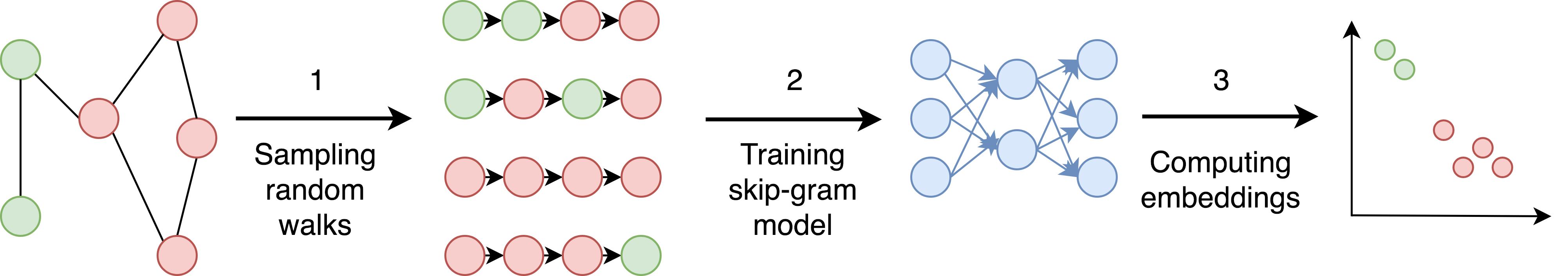 22 |
23 | Unsupervised online learning approach, inspired from word2vec in NLP, but, here the goal is to generate node embeddings.
24 | - [DeepWalk Blog](https://dsgiitr.in/blogs/deepwalk)
25 | - [Jupyter Notebook](https://github.com/dsgiitr/graph_nets/blob/master/DeepWalk/DeepWalk_Blog%2BCode.ipynb)
26 | - [Code](https://github.com/dsgiitr/graph_nets/blob/master/DeepWalk/DeepWalk.py)
27 | - [Paper -> DeepWalk: Online Learning of Social Representations](https://arxiv.org/abs/1403.6652)
28 |
29 |
30 |
22 |
23 | Unsupervised online learning approach, inspired from word2vec in NLP, but, here the goal is to generate node embeddings.
24 | - [DeepWalk Blog](https://dsgiitr.in/blogs/deepwalk)
25 | - [Jupyter Notebook](https://github.com/dsgiitr/graph_nets/blob/master/DeepWalk/DeepWalk_Blog%2BCode.ipynb)
26 | - [Code](https://github.com/dsgiitr/graph_nets/blob/master/DeepWalk/DeepWalk.py)
27 | - [Paper -> DeepWalk: Online Learning of Social Representations](https://arxiv.org/abs/1403.6652)
28 |
29 |
30 |  32 |
33 | GCNs draw on the idea of Convolution Neural Networks re-defining them for the non-euclidean data domain. They are convolutional, because filter parameters are typically shared over all locations in the graph unlike typical GNNs.
34 | - [GCN Blog](https://dsgiitr.in/blogs/gcn)
35 | - [Jupyter Notebook](https://github.com/dsgiitr/graph_nets/blob/master/GCN/GCN_Blog%2BCode.ipynb)
36 | - [Code](https://github.com/dsgiitr/graph_nets/blob/master/GCN/GCN.py)
37 | - [Paper -> Semi-Supervised Classification with Graph Convolutional Networks](https://arxiv.org/abs/1609.02907)
38 |
39 |
40 |
32 |
33 | GCNs draw on the idea of Convolution Neural Networks re-defining them for the non-euclidean data domain. They are convolutional, because filter parameters are typically shared over all locations in the graph unlike typical GNNs.
34 | - [GCN Blog](https://dsgiitr.in/blogs/gcn)
35 | - [Jupyter Notebook](https://github.com/dsgiitr/graph_nets/blob/master/GCN/GCN_Blog%2BCode.ipynb)
36 | - [Code](https://github.com/dsgiitr/graph_nets/blob/master/GCN/GCN.py)
37 | - [Paper -> Semi-Supervised Classification with Graph Convolutional Networks](https://arxiv.org/abs/1609.02907)
38 |
39 |
40 |  42 |
43 | Previous approaches are transductive and don't naturally generalize to unseen nodes. GraphSAGE is an inductive framework leveraging node feature information to efficiently generate node embeddings.
44 | - [GraphSAGE Blog](https://dsgiitr.in/blogs/graphsage)
45 | - [Jupyter Notebook](https://github.com/dsgiitr/graph_nets/blob/master/GraphSAGE/GraphSAGE_Code%2BBlog.ipynb)
46 | - [Code](https://github.com/dsgiitr/graph_nets/blob/master/GraphSAGE/GraphSAGE.py)
47 | - [Paper -> Inductive Representation Learning on Large Graphs](https://arxiv.org/abs/1706.02216)
48 |
49 |
50 |
42 |
43 | Previous approaches are transductive and don't naturally generalize to unseen nodes. GraphSAGE is an inductive framework leveraging node feature information to efficiently generate node embeddings.
44 | - [GraphSAGE Blog](https://dsgiitr.in/blogs/graphsage)
45 | - [Jupyter Notebook](https://github.com/dsgiitr/graph_nets/blob/master/GraphSAGE/GraphSAGE_Code%2BBlog.ipynb)
46 | - [Code](https://github.com/dsgiitr/graph_nets/blob/master/GraphSAGE/GraphSAGE.py)
47 | - [Paper -> Inductive Representation Learning on Large Graphs](https://arxiv.org/abs/1706.02216)
48 |
49 |
50 |  52 |
53 | ChebNet is a formulation of CNNs in the context of spectral graph theory.
54 | - [ChebNet Blog](https://dsgiitr.in/blogs/chebnet/)
55 | - [Jupyter Notebook](https://github.com/dsgiitr/graph_nets/blob/master/ChebNet/Chebnet_Blog%2BCode.ipynb)
56 | - [Code](https://github.com/dsgiitr/graph_nets/blob/master/ChebNet/coarsening.py)
57 | - [Paper -> Convolutional Neural Networks on Graphs with Fast Localized Spectral Filtering](https://arxiv.org/abs/1606.09375)
58 |
59 |
52 |
53 | ChebNet is a formulation of CNNs in the context of spectral graph theory.
54 | - [ChebNet Blog](https://dsgiitr.in/blogs/chebnet/)
55 | - [Jupyter Notebook](https://github.com/dsgiitr/graph_nets/blob/master/ChebNet/Chebnet_Blog%2BCode.ipynb)
56 | - [Code](https://github.com/dsgiitr/graph_nets/blob/master/ChebNet/coarsening.py)
57 | - [Paper -> Convolutional Neural Networks on Graphs with Fast Localized Spectral Filtering](https://arxiv.org/abs/1606.09375)
58 |
59 |  63 |
64 | GAT is able to attend over their neighborhoods’ features, implicitly specifying different weights to different nodes in a neighborhood, without requiring any kind of costly matrix operation or depending on knowing the graph structure upfront.
65 | - [GAT Blog](https://dsgiitr.in/blogs/gat)
66 | - [Jupyter Notebook](https://github.com/dsgiitr/graph_nets/blob/master/GAT/GAT_Blog%2BCode.ipynb)
67 | - [Code](https://github.com/dsgiitr/graph_nets/blob/master/GAT/GAT_PyG.py)
68 | - [Paper -> Graph Attention Networks](https://arxiv.org/abs/1710.10903)
69 |
70 |
63 |
64 | GAT is able to attend over their neighborhoods’ features, implicitly specifying different weights to different nodes in a neighborhood, without requiring any kind of costly matrix operation or depending on knowing the graph structure upfront.
65 | - [GAT Blog](https://dsgiitr.in/blogs/gat)
66 | - [Jupyter Notebook](https://github.com/dsgiitr/graph_nets/blob/master/GAT/GAT_Blog%2BCode.ipynb)
67 | - [Code](https://github.com/dsgiitr/graph_nets/blob/master/GAT/GAT_PyG.py)
68 | - [Paper -> Graph Attention Networks](https://arxiv.org/abs/1710.10903)
69 |
70 |