├── DataSelection
├── 2.DataPreparation
│ └── data_preparation.ipynb
├── 3.ExploreLATData
│ └── explore_latdata.ipynb
├── 4.ExploreLATDataBurst
│ └── explore_latdata_burst.ipynb
└── 5.UsingLATAllSkyWeekly
│ └── LAT_weekly_allsky.ipynb
├── Exposure
└── Exposure.ipynb
├── GRBAnalysis
└── 1.LATGRBAnalysis
│ └── lat_grb_analysis.ipynb
├── LICENSE
├── ObsSim
├── 1.ObservationSim
│ └── obssim_tutorial.ipynb
└── 2.OrbitSim
│ └── orbsim_tutorial.ipynb
├── README.md
└── SourceAnalysis
├── 1.BinnedLikelihood
└── binned_likelihood_tutorial.ipynb
├── 10.EnergyDispersion
└── binnededisp_tutorial.ipynb
├── 2.UnbinnedLikelihood
└── likelihood_tutorial.ipynb
├── 3.PythonLikelihood
└── python_tutorial.ipynb
├── 3C279_input_model.xml
├── 4.SummedPythonLikelihood
└── summed_tutorial.ipynb
├── 5.PythonUpperLimits
└── upper_limits.ipynb
├── 6.ExtendedSourceAnalysis
└── extended.ipynb
├── 7.LATAperturePhotometry
└── aperture_photometry.ipynb
└── 8.PulsarGating
└── pulsar_gating_tutorial.ipynb
/DataSelection/2.DataPreparation/data_preparation.ipynb:
--------------------------------------------------------------------------------
1 | {
2 | "cells": [
3 | {
4 | "cell_type": "markdown",
5 | "metadata": {},
6 | "source": [
7 | "# Data Preparation\n",
8 | "\n",
9 | "Photon and spacecraft data are all that a user needs for the analysis. For the definition of LAT data products, see the information in the [Cicerone](https://fermi.gsfc.nasa.gov/ssc/data/analysis/documentation/Cicerone/Cicerone_Data/LAT_DP.html).\n",
10 | "\n",
11 | "The LAT data can be extracted from the Fermi Science Support Center web site as described in the section [Extract LAT data](https://fermi.gsfc.nasa.gov/ssc/data/analysis/scitools/extract_latdata.html). Preparing these data for analysis depends on the type of analysis you wish to perform (e.g. point source, extended source, GRB spectral analysis, timing analysis, etc). The different cuts to the data are described in detail in the [Cicerone](https://fermi.gsfc.nasa.gov/ssc/data/analysis/documentation/Cicerone/Cicerone_Data/LAT_DP.html)."
12 | ]
13 | },
14 | {
15 | "cell_type": "markdown",
16 | "metadata": {},
17 | "source": [
18 | "Data preparation consists of two steps:\n",
19 | "* ([gtselect](https://fermi.gsfc.nasa.gov/ssc/data/analysis/scitools/help/gtselect.txt)): Used to make cuts based on columns in the event data file such as time, energy, position, zenith angle, instrument coordinates, event class, and event type (new in Pass 8).\n",
20 | "* ([gtmktime](https://fermi.gsfc.nasa.gov/ssc/data/analysis/scitools/help/gtmktime.txt)): In addition to cutting the selected events, gtmktime makes cuts based on the spacecraft file and updates the Good Time Interval (GTI) extension.\n",
21 | "\n",
22 | "\n",
23 | "Here we give an example of how to prepare the data for the analysis of a point source. For your particular source analysis you have to prepare your data performing similar steps, but with the cuts suggested in Cicerone for your case."
24 | ]
25 | },
26 | {
27 | "cell_type": "markdown",
28 | "metadata": {},
29 | "source": [
30 | "## 1. Event Selection with gtselect\n",
31 | "\n",
32 | "In this section, we look at making basic data cuts using [gtselect](https://fermi.gsfc.nasa.gov/ssc/data/analysis/scitools/help/gtselect.txt). By default, gtselect prompts for cuts on:\n",
33 | "* Time\n",
34 | "* Energy\n",
35 | "* Position (RA,Dec,radius)\n",
36 | "* Maximum Zenith Angle\n",
37 | "\n",
38 | "However, by using the following hidden parameters (or using the '_Show Advanced Parameters_' check box in GUI mode), you can also make cuts on:\n",
39 | "\n",
40 | "* Minimum Event class ID (``evclsmin``)\n",
41 | "* Maximum Event class ID (``evclsmax``)\n",
42 | "* Event conversion type ID (``convtype``)\n",
43 | "* Minimum pulse phase (``phasemin``)\n",
44 | "* Maximum pulse phase (``phasemax``)"
45 | ]
46 | },
47 | {
48 | "cell_type": "markdown",
49 | "metadata": {},
50 | "source": [
51 | "For this example, we use data that was extracted using the procedure described in the [Extract LAT Data](https://fermi.gsfc.nasa.gov/ssc/data/analysis/scitools/extract_latdata.html) tutorial. The original selection used the following information:\n",
52 | "\n",
53 | "* Search Center (RA,DEC) = (193.98,-5.82)\n",
54 | "* Radius = 20 degrees\n",
55 | "* Start Time (MET) = 239557417 seconds (2008-08-04 T15:43:37)\n",
56 | "* Stop Time (MET) = 255398400 seconds (2009-02-04 T00:00:00)\n",
57 | "* Minimum Energy = 100 MeV\n",
58 | "* Maximum Energy = 500000 MeV\n",
59 | "\n",
60 | "The LAT operated in survey mode for that period of time. We provide the user with the photon and spacecraft data files extracted in the same method as described in the [Extract LAT data](https://fermi.gsfc.nasa.gov/ssc/data/analysis/scitools/extract_latdata.html) tutorial:\n",
61 | "\n",
62 | "1. L1506091032539665347F73_PH00.fits\n",
63 | "2. L1506091032539665347F73_PH01.fits\n",
64 | "3. L1506091032539665347F73_SC00.fits"
65 | ]
66 | },
67 | {
68 | "cell_type": "code",
69 | "execution_count": null,
70 | "metadata": {},
71 | "outputs": [],
72 | "source": [
73 | "!wget https://fermi.gsfc.nasa.gov/ssc/data/analysis/scitools/data/dataPreparation/L1506091032539665347F73_PH00.fits\n",
74 | "!wget https://fermi.gsfc.nasa.gov/ssc/data/analysis/scitools/data/dataPreparation/L1506091032539665347F73_PH01.fits\n",
75 | "!wget https://fermi.gsfc.nasa.gov/ssc/data/analysis/scitools/data/dataPreparation/L1506091032539665347F73_SC00.fits"
76 | ]
77 | },
78 | {
79 | "cell_type": "code",
80 | "execution_count": null,
81 | "metadata": {},
82 | "outputs": [],
83 | "source": [
84 | "!mkdir data\n",
85 | "!mv *.fits ./data"
86 | ]
87 | },
88 | {
89 | "cell_type": "markdown",
90 | "metadata": {},
91 | "source": [
92 | "If more than one photon file was returned by the [LAT Data Server](https://fermi.gsfc.nasa.gov/cgi-bin/ssc/LAT/LATDataQuery.cgi), we will need to provide an input file list in order to use all the event data files in the same analysis. This text file can be generated by typing:"
93 | ]
94 | },
95 | {
96 | "cell_type": "code",
97 | "execution_count": null,
98 | "metadata": {},
99 | "outputs": [],
100 | "source": [
101 | "!ls ./data/*_PH* > ./data/events.txt"
102 | ]
103 | },
104 | {
105 | "cell_type": "code",
106 | "execution_count": null,
107 | "metadata": {
108 | "scrolled": true
109 | },
110 | "outputs": [],
111 | "source": [
112 | "!cat ./data/events.txt"
113 | ]
114 | },
115 | {
116 | "cell_type": "markdown",
117 | "metadata": {},
118 | "source": [
119 | "This input file list can be used in place of a single input events (or FT1) file by placing an `@` symbol before the text filename. The output from [gtselect](https://fermi.gsfc.nasa.gov/ssc/data/analysis/scitools/help/gtselect.txt) will be a single file containing all events from the combined file list that satisfy the other specified cuts.\n",
120 | "\n",
121 | "For a simple point source analysis, it is recommended that you only include events with a high probability of being photons. This cut is performed by selecting \"source\" class events with the the [gtselect](https://fermi.gsfc.nasa.gov/ssc/data/analysis/scitools/help/gtselect.txt) tool by including the hidden parameter ``evclass`` on the command line. For LAT Pass 8 data, `source` events are specified as event class 128 (the default value).\n",
122 | "\n",
123 | "Additionally, in Pass 8, you can supply the hidden parameter `evtype` (event type) which is a sub-selection on `evclass`. For a simple analysis, we wish to include all front+back converting events within all PSF and Energy subclasses. This is specified as `evtype` 3 (the default value).\n",
124 | "\n",
125 | "The recommended values for both `evclass` and `evtype` may change as LAT data processing develops.\n",
126 | "\n",
127 | "Now run [gtselect](https://fermi.gsfc.nasa.gov/ssc/data/analysis/scitools/help/gtselect.txt) to select the data you wish to analyze. For this example, we consider the \"source class\" photons within a 20 degree acceptance cone of the blazar 3C 279. We apply the **gtselect** tool to the data file as follows:"
128 | ]
129 | },
130 | {
131 | "cell_type": "code",
132 | "execution_count": null,
133 | "metadata": {},
134 | "outputs": [],
135 | "source": [
136 | "%%bash\n",
137 | "gtselect evclass=128 evtype=3\n",
138 | " @./data/events.txt\n",
139 | " ./data/3C279_region_filtered.fits\n",
140 | " 193.98\n",
141 | " -5.82\n",
142 | " 20\n",
143 | " INDEF\n",
144 | " INDEF\n",
145 | " 100\n",
146 | " 500000\n",
147 | " 90\n",
148 | "\n",
149 | "#### Parameters:\n",
150 | "# Input file or files (if multiple files are in a .txt file,\n",
151 | "# don't forget the @ symbol)\n",
152 | "# Output file\n",
153 | "# RA for new search center\n",
154 | "# Dec or new search center\n",
155 | "# Radius of the new search region\n",
156 | "# Start time (MET in s)\n",
157 | "# End time (MET in s)\n",
158 | "# Lower energy limit (MeV)\n",
159 | "# Upper energy limit (MeV)\n",
160 | "# Maximum zenith angle value (degrees)"
161 | ]
162 | },
163 | {
164 | "cell_type": "markdown",
165 | "metadata": {},
166 | "source": [
167 | "The filtered data will be found in the file `./data/3C279_region_filtered.fits`.\n",
168 | "\n",
169 | "**Note**: If you don't want to make a selection on a given parameter, just enter a zero (0) as the value.\n",
170 | "\n",
171 | "In this step we also selected the maximum zenith angle value as suggested in the [Cicerone](https://fermi.gsfc.nasa.gov/ssc/data/analysis/documentation/Cicerone/Cicerone_Data_Exploration/Data_preparation.html). Gamma-ray photons coming from the Earth limb (\"albedo gammas\") are a strong source of background. You can minimize this effect with a zenith angle cut. The value of `zmax` = 90 degrees is suggested for reconstructing events above 100 MeV and provides a sufficient buffer between your region of interest (ROI) and the Earth's limb.\n",
172 | "\n",
173 | "In the next step, [gtmktime](https://fermi.gsfc.nasa.gov/ssc/data/analysis/scitools/help/gtmktime.txt) will remove any time period for which our ROI overlaps this buffer region. While increasing the buffer (reducing `zmax`) may decrease the background rate from albedo gammas, it will also reduce the amount of time your ROI is completely free of the buffer zone and thus reduce the livetime on the source of interest."
174 | ]
175 | },
176 | {
177 | "cell_type": "markdown",
178 | "metadata": {},
179 | "source": [
180 | "**Notes**:\n",
181 | "\n",
182 | "* The RA and Dec of the search center must exactly match that used in the dataserver selection. If they are not the same, multiple copies of the source position will appear in your prepared data file which will cause later stages of analysis to fail. See \"DSS Keywords\" below.\n",
183 | "\n",
184 | "\n",
185 | "* The radius of the search region selected here must lie entirely within the region defined in the dataserver selection. They can be the same values, with no negative effects.\n",
186 | "\n",
187 | "\n",
188 | "* The time span selected here must lie within the time span defined in the dataserver selection. They can be the same values with no negative effects.\n",
189 | "\n",
190 | "\n",
191 | "* The energy range selected here must lie within the time span defined in the dataserver selection. They can be the same values with no negative effects."
192 | ]
193 | },
194 | {
195 | "cell_type": "markdown",
196 | "metadata": {},
197 | "source": [
198 | "**BE AWARE**: [gtselect](https://fermi.gsfc.nasa.gov/ssc/data/analysis/scitools/help/gtselect.txt) writes descriptions of the data selections to a series of _Data Sub-Space_ (DSS) keywords in the `EVENTS` extension header.\n",
199 | "\n",
200 | "These keywords are used by the exposure-related tools and by [gtlike](https://fermi.gsfc.nasa.gov/ssc/data/analysis/scitools/help/gtlike.txt) for calculating various quantities, such as the predicted number of detected events given by the source model. These keywords MUST be same for all of the filtered event files considered in a given analysis.\n",
201 | "\n",
202 | "[gtlike](https://fermi.gsfc.nasa.gov/ssc/data/analysis/scitools/help/gtlike.txt) will check to ensure that all of the DSS keywords are the same in all of the event data files. For a discussion of the DSS keywords see the [Data Sub-Space Keywords page](https://fermi.gsfc.nasa.gov/ssc/data/analysis/scitools/dss_keywords.html)."
203 | ]
204 | },
205 | {
206 | "cell_type": "markdown",
207 | "metadata": {},
208 | "source": [
209 | "There are multiple ways to view information about your data file. For example:\n",
210 | "* You may obtain the value of start and end time of your file by using the fkeypar tool. This tool is part of the [FTOOLS](http://heasarc.nasa.gov/lheasoft/ftools/ftools_menu.html) software package and is used to read the value of a FITS header keyword and write it to an output parameter file. For more information on `fkeypar`, type: "
211 | ]
212 | },
213 | {
214 | "cell_type": "markdown",
215 | "metadata": {},
216 | "source": [
217 | "`fhelp fkeypar`"
218 | ]
219 | },
220 | {
221 | "cell_type": "markdown",
222 | "metadata": {},
223 | "source": [
224 | "* The [gtvcut](https://fermi.gsfc.nasa.gov/ssc/data/analysis/scitools/help/gtvcut.txt) tool can be used to view the DSS keywords in a given extension, where the EVENTS extension is assumed by default. This is an excellent way to to find out what selections have been made already on your data file (by either the dataserver, or previous runs of gtselect).\n",
225 | "\n",
226 | " * NOTE: If you wish to view the (very long) list of good time intervals (GTIs), you can use the hidden parameter `suppress_gtis=no` on the command line. The full list of GTIs is suppressed by default."
227 | ]
228 | },
229 | {
230 | "cell_type": "markdown",
231 | "metadata": {},
232 | "source": [
233 | "## 2. Time Selection with gtmktime\n",
234 | "\n",
235 | "Good Time Intervals (GTIs):\n",
236 | "\n",
237 | "* A GTI is a time range when the data can be considered valid. The GTI extension contains a list of these GTI's for the file. Thus the sum of the entries in the GTI extension of a file corresponds to the time when the data in the file is \"good.\"\n",
238 | "\n",
239 | "* The initial list of GTI's are the times that the LAT was collecting data over the time range you selected. The LAT does not collect data while the observatory is transiting the South Atlantic Anomaly (SAA), or during rare events such as software updates or spacecraft maneuvers.\n",
240 | "\n",
241 | "**Notes**:\n",
242 | "* Your object will most likely not be in the field of view during the entire time that the LAT was taking data.\n",
243 | "\n",
244 | "* Additional data cuts made with gtmktime will update the GTIs based on the cuts specified in both gtmktime and gtselect.\n",
245 | "\n",
246 | "* The Fermitools use the GTIs when calculating exposure. If the GTIs have not been properly updated, the exposure correction made during science analysis may be incorrect."
247 | ]
248 | },
249 | {
250 | "cell_type": "markdown",
251 | "metadata": {},
252 | "source": [
253 | "[gtmktime](https://fermi.gsfc.nasa.gov/ssc/data/analysis/scitools/help/gtmktime.txt) is used to update the GTI extension and make cuts based on spacecraft parameters contained in the spacecraft (pointing and livetime history) file. It reads the spacecraft file and, based on the filter expression and specified cuts, creates a set of GTIs. These are then combined (logical and) with the existing GTIs in the Event data file, and all events outside this new set of GTIs are removed from the file. New GTIs are then written to the GTI extension of the new file.\n",
254 | "\n",
255 | "Cuts can be made on any field in the spacecraft file by adding terms to the filter expression using C-style relational syntax:\n",
256 | "\n",
257 | " ! -> not, && -> and, || -> or, ==, !=, >, <, >=, <=\n",
258 | "\n",
259 | " ABS(), COS(), SIN(), etc., also work\n",
260 | "\n",
261 | ">**NOTE**: Every time you specify an additional cut on time, ROI, zenith angle, event class, or event type using [gtselect](https://fermi.gsfc.nasa.gov/ssc/data/analysis/scitools/help/gtselect.txt), you must run [gtmktime](https://fermi.gsfc.nasa.gov/ssc/data/analysis/scitools/help/gtmktime.txt) to reevaluate the GTI selection.\n",
262 | "\n",
263 | "Several of the cuts made above with **gtselect** will directly affect the exposure. Running [gtmktime](https://fermi.gsfc.nasa.gov/ssc/data/analysis/scitools/help/gtmktime.txt) will select the correct GTIs to handle these cuts."
264 | ]
265 | },
266 | {
267 | "cell_type": "markdown",
268 | "metadata": {},
269 | "source": [
270 | "It is also especially important to apply a zenith cut for small ROIs (< 20 degrees), as this brings your source of interest close to the Earth's limb. There are two different methods for handling the complex cut on zenith angle:\n",
271 | "\n",
272 | "* One method is to exclude time intervals where the buffer zone defined by the zenith cut intersects the ROI from the list of GTIs. In order to do that, run [gtmktime](https://fermi.gsfc.nasa.gov/ssc/data/analysis/scitools/help/gtmktime.txt) and answer \"yes\" at the prompt:"
273 | ]
274 | },
275 | {
276 | "cell_type": "markdown",
277 | "metadata": {},
278 | "source": [
279 | "```\n",
280 | "> gtmktime\n",
281 | "...\n",
282 | "> Apply ROI-based zenith angle cut [] yes\n",
283 | "```"
284 | ]
285 | },
286 | {
287 | "cell_type": "markdown",
288 | "metadata": {},
289 | "source": [
290 | ">**NOTE**: If you are studying a very broad region (or the whole sky) you would lose most (all) of your data when you implement the ROI-based zenith angle cut in [gtmktime](https://fermi.gsfc.nasa.gov/ssc/data/analysis/scitools/help/gtmktime.txt).\n",
291 | ">\n",
292 | ">In this case you can allow all time intervals where the cut intersects the ROI, but the intersection lies outside the FOV. To do this, run _gtmktime_ specifying a filter expression defining your analysis region, and answer \"no\" to the question regarding the ROI-based zenith angle cut:\n",
293 | ">\n",
294 | ">`> Apply ROI-based zenith angle cut [] no`\n",
295 | ">\n",
296 | ">Here, RA_of_center_ROI, DEC_of_center_ROI and radius_ROI correspond to the ROI selection made with gtselect, zenith_cut is defined as 90 degrees (as above), and limb_angle_minus_FOV is (zenith angle of horizon - FOV radius) where the zenith angle of the horizon is 113 degrees."
297 | ]
298 | },
299 | {
300 | "cell_type": "markdown",
301 | "metadata": {},
302 | "source": [
303 | "* Alternatively, you can apply the zenith cut to the livetime calculation while running [gtltcube](https://fermi.gsfc.nasa.gov/ssc/data/analysis/scitools/help/gtltcube.txt). This is the method that is currently recommended by the LAT team (see the [Livetimes and Exposure](https://fermi.gsfc.nasa.gov/ssc/data/analysis/documentation/Cicerone/Cicerone_Likelihood/Exposure.html) section of the [Cicerone](https://fermi.gsfc.nasa.gov/ssc/data/analysis/documentation/Cicerone/)), and is the method we will use most commonly in these analysis threads. To do this, answer \"no\" at the [gtmktime](https://fermi.gsfc.nasa.gov/ssc/data/analysis/scitools/help/gtmktime.txt) prompt:"
304 | ]
305 | },
306 | {
307 | "cell_type": "markdown",
308 | "metadata": {},
309 | "source": [
310 | "`> Apply ROI-based zenith angle cut [] no`\n",
311 | "\n",
312 | "You'll then need to specify a value for gtltcube's `zmax` parameter when calculating the livetime cube:\n",
313 | "\n",
314 | "`> gtltcube zmax=90`"
315 | ]
316 | },
317 | {
318 | "cell_type": "markdown",
319 | "metadata": {},
320 | "source": [
321 | "[gtmktime](https://fermi.gsfc.nasa.gov/ssc/data/analysis/scitools/help/gtmktime.txt) also provides the ability to exclude periods when some event has negatively affected the quality of the LAT data. To do this, we select good time intervals (GTIs) by using a logical filter for any of the [quantities in the spacecraft file](https://fermi.gsfc.nasa.gov/ssc/data/analysis/documentation/Cicerone/Cicerone_Data/LAT_Data_Columns.html#SpacecraftFile). Some possible quantities for filtering data are:\n",
322 | "\n",
323 | "* `DATA_QUAL` - quality flag set by the LAT instrument team (1 = ok, 2 = waiting review, 3 = good with bad parts, 0 = bad)\n",
324 | "\n",
325 | "* `LAT_CONFIG` - instrument configuration (0 = not recommended for analysis, 1 = science configuration)\n",
326 | "\n",
327 | "* `ROCK_ANGLE` - can be used to eliminate pointed observations from the dataset.\n",
328 | "\n",
329 | ">**NOTE**: A history of the rocking profiles that have been used by the LAT can be found in the [SSC's LAT observations page.](https://fermi.gsfc.nasa.gov/ssc/observations/types/allsky/)"
330 | ]
331 | },
332 | {
333 | "cell_type": "markdown",
334 | "metadata": {},
335 | "source": [
336 | "The current [gtmktime](https://fermi.gsfc.nasa.gov/ssc/data/analysis/scitools/help/gtmktime.txt) filter expression recommended by the LAT team is:\n",
337 | "\n",
338 | "**(DATA_QUAL>0)&&(LAT_CONFIG==1).**\n",
339 | "\n",
340 | ">**NOTE**: The \"DATA_QUAL\" parameter can be set to different values, based on the type of object and analysis the user is interested into (see this page of the Cicerone for the most updated detailed description of the parameter's values). Typically, setting the parameter to 1 is the best option. For GRB analysis, on the contrary, the parameter should be set to \">0\".\n",
341 | "\n",
342 | "Here is an example of running [gtmktime](https://fermi.gsfc.nasa.gov/ssc/data/analysis/scitools/help/gtmktime.txt) on the 3C 279 filtered events file. For convienience, we rename the spacecraft file to `spacecraft.fits`."
343 | ]
344 | },
345 | {
346 | "cell_type": "code",
347 | "execution_count": null,
348 | "metadata": {},
349 | "outputs": [],
350 | "source": [
351 | "!mv ./data/L1506091032539665347F73_SC00.fits ./data/spacecraft.fits"
352 | ]
353 | },
354 | {
355 | "cell_type": "markdown",
356 | "metadata": {},
357 | "source": [
358 | "Now, we run **gtmktime**:"
359 | ]
360 | },
361 | {
362 | "cell_type": "code",
363 | "execution_count": null,
364 | "metadata": {},
365 | "outputs": [],
366 | "source": [
367 | "%%bash\n",
368 | "gtmktime\n",
369 | " ./data/spacecraft.fits\n",
370 | " (DATA_QUAL>0)&&(LAT_CONFIG==1)\n",
371 | " no\n",
372 | " ./data/3C279_region_filtered.fits\n",
373 | " ./data/3C279_region_filtered_gti.fits\n",
374 | " \n",
375 | "#### Parameters specified above are:\n",
376 | "# Spacecraft file\n",
377 | "# Filter expression\n",
378 | "# Apply ROI-based zenith angle cut\n",
379 | "# Event data file\n",
380 | "# Output event file name"
381 | ]
382 | },
383 | {
384 | "cell_type": "code",
385 | "execution_count": null,
386 | "metadata": {},
387 | "outputs": [],
388 | "source": [
389 | "!ls ./data/"
390 | ]
391 | },
392 | {
393 | "cell_type": "markdown",
394 | "metadata": {},
395 | "source": [
396 | "The filtered event file, [3C279_region_filtered_gti.fits,](https://fermi.gsfc.nasa.gov/ssc/data/analysis/scitools/data/dataPreparation/3C279_region_filtered_gti.fits) output from [gtmktime](https://fermi.gsfc.nasa.gov/ssc/data/analysis/scitools/help/gtmktime.txt) can be downloaded from the Fermi SSC site.\n",
397 | "\n",
398 | "After the data preparation, it is advisable to examine your data before beginning detailed analysis. The [Explore LAT data](3.ExploreLATData.ipynb) tutorial has suggestions on methods of getting a quick preview of your data."
399 | ]
400 | }
401 | ],
402 | "metadata": {
403 | "kernelspec": {
404 | "display_name": "Python 3",
405 | "language": "python",
406 | "name": "python3"
407 | },
408 | "language_info": {
409 | "codemirror_mode": {
410 | "name": "ipython",
411 | "version": 3
412 | },
413 | "file_extension": ".py",
414 | "mimetype": "text/x-python",
415 | "name": "python",
416 | "nbconvert_exporter": "python",
417 | "pygments_lexer": "ipython3",
418 | "version": "3.7.9"
419 | },
420 | "pycharm": {
421 | "stem_cell": {
422 | "cell_type": "raw",
423 | "metadata": {
424 | "collapsed": false
425 | },
426 | "source": []
427 | }
428 | }
429 | },
430 | "nbformat": 4,
431 | "nbformat_minor": 2
432 | }
433 |
--------------------------------------------------------------------------------
/DataSelection/3.ExploreLATData/explore_latdata.ipynb:
--------------------------------------------------------------------------------
1 | {
2 | "cells": [
3 | {
4 | "cell_type": "markdown",
5 | "metadata": {},
6 | "source": [
7 | "# Exploring LAT Data\n",
8 | "\n",
9 | "Before detailed analysis, we recommended gaining familiarity with the structure and content of the [LAT data products](https://fermi.gsfc.nasa.gov/ssc/data/analysis/documentation/Cicerone/Cicerone_Data/LAT_DP.html), as well as the process for [preparing the data](https://fermi.gsfc.nasa.gov/ssc/data/analysis/scitools/data_preparation.html) by making cuts on the data file. This tutorial demonstrates simple ways to quickly explore LAT data.\n",
10 | "\n",
11 | ">**IMPORTANT**! In almost all cases, light curves and energy spectra need to be produced by a [Likelihood Analysis](https://fermi.gsfc.nasa.gov/ssc/data/analysis/scitools/binned_likelihood_tutorial.html) using [gtlike](https://fermi.gsfc.nasa.gov/ssc/data/analysis/scitools/help/gtlike.txt) to be scientifically valid.\n",
12 | "\n",
13 | "In addition to the Fermitools, you will also be using the following FITS File Viewers:\n",
14 | "\n",
15 | "* _ds9_ (image viewer); download and install from: http://ds9.si.edu/site/Home.html\n",
16 | "\n",
17 | "* _fv_ (view images and tables; can also make plots and histograms;\n",
18 | "download and install from: http://heasarc.gsfc.nasa.gov/docs/software/ftools/fv"
19 | ]
20 | },
21 | {
22 | "cell_type": "markdown",
23 | "metadata": {},
24 | "source": [
25 | "## Data Files\n",
26 | "\n",
27 | "Some of the files used in this tutorial were prepared within the [Data Preparation](https://fermi.gsfc.nasa.gov/ssc/data/analysis/scitools/data_preparation.html) tutorial. These are:\n",
28 | "\n",
29 | "* [`3C279_region_filtered_gti.fits`](https://fermi.gsfc.nasa.gov/ssc/data/analysis/scitools/data/dataPreparation/3C279_region_filtered_gti.fits) (16.6 MB) - a 20 degree region around the blazar 3C 279 with appropriate selection cuts applied\n",
30 | "* [`spacecraft.fits`](https://fermi.gsfc.nasa.gov/ssc/data/analysis/scitools/data/dataPreparation/spacecraft.fits) (67.6 MB) - the spacecraft data file for 3C 279.\n",
31 | "\n",
32 | "You can retrieve these via `wget`. Below we download these data files and move them to a `data` subdirectory:"
33 | ]
34 | },
35 | {
36 | "cell_type": "code",
37 | "execution_count": null,
38 | "metadata": {},
39 | "outputs": [],
40 | "source": [
41 | "!wget \"https://fermi.gsfc.nasa.gov/ssc/data/analysis/scitools/data/exploreLATData/3C279_region_filtered_gti.fits\"\n",
42 | "!wget \"https://fermi.gsfc.nasa.gov/ssc/data/analysis/scitools/data/exploreLATData/spacecraft.fits\""
43 | ]
44 | },
45 | {
46 | "cell_type": "code",
47 | "execution_count": null,
48 | "metadata": {},
49 | "outputs": [],
50 | "source": [
51 | "!mkdir ./data\n",
52 | "!mv *.fits ./data"
53 | ]
54 | },
55 | {
56 | "cell_type": "markdown",
57 | "metadata": {},
58 | "source": [
59 | "Alternatively, you can select your own region and time period of interest from the [LAT data server](http://fermi.gsfc.nasa.gov/cgi-bin/ssc/LAT/LATDataQuery.cgi) and substitute them. **Photon** and **spacecraft** data files are all that you need for the analysis."
60 | ]
61 | },
62 | {
63 | "cell_type": "markdown",
64 | "metadata": {},
65 | "source": [
66 | "# 1. Using `ds9`\n",
67 | "\n",
68 | "First, we'll look at making quick counts maps with *ds9*."
69 | ]
70 | },
71 | {
72 | "cell_type": "markdown",
73 | "metadata": {},
74 | "source": [
75 | "### *ds9* Quick look:\n",
76 | "\n",
77 | "To see the data, use *ds9* to create a quick counts maps of the events in the file.\n",
78 | "\n",
79 | "For example, to look at the 3C 279 data file, type the following command in your command line:"
80 | ]
81 | },
82 | {
83 | "cell_type": "markdown",
84 | "metadata": {},
85 | "source": [
86 | "```\n",
87 | "> ds9 -bin factor 0.1 0.1 -cmap b -scale sqrt 3C279_region_filtered_gti.fits &\n",
88 | "```"
89 | ]
90 | },
91 | {
92 | "cell_type": "markdown",
93 | "metadata": {},
94 | "source": [
95 | "A *ds9* window will open up and an image similar to the one shown below will be displayed.\n",
96 | "\n",
97 | "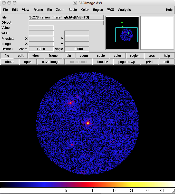\n",
98 | "\n",
99 | "\n",
100 | "Breaking the command line into its parts:\n",
101 | "\n",
102 | "* *ds9* - executes the *ds9* application.\n",
103 | "\n",
104 | "* -bin factor 0.1 0.1 - Tells *ds9* that the x and y bin sizes are to be 0.1 units in each direction. Since we will be binning on the coordinates (RA, DEC), this means we will have 0.1 degree bins.\n",
105 | "\n",
106 | ">**Note**: The default factor is 1, so if you leave this off the *ds9* command line the image will use 1 degree bins\n",
107 | "\n",
108 | "* -cmap b - Tells ds9 to use the \"b\" color map to display the image. This is completely optional and the choice of map \"b\" represents the personal preference of the author. If left off, the default color map is \"gray\" (a grayscale color map).\n",
109 | "\n",
110 | "\n",
111 | "* -scale sqrt - Tells *ds9* to scale the colormap using the square root of the counts in the pixels. This particular scale helps to accentuate faint maxima where there is a bright source in the field as is the case here. Again this is the author's personal preference for this option. If left off, the default scale is linear.\n",
112 | "\n",
113 | "\n",
114 | "* & - backgrounds the task, allowing continued use of the command line."
115 | ]
116 | },
117 | {
118 | "cell_type": "markdown",
119 | "metadata": {},
120 | "source": [
121 | "### Exploring with fv:\n",
122 | "\n",
123 | "*fv* gives you much more interactive control of how you explore the data.\n",
124 | "\n",
125 | "It can make plots and 1D and 2D histograms, allow you look at the data directly, and enable you to view the FITS file headers to look at some of the important keywords.\n",
126 | "\n",
127 | "To display a file in *fv*, type *fv* and the filename in the command line:"
128 | ]
129 | },
130 | {
131 | "cell_type": "markdown",
132 | "metadata": {},
133 | "source": [
134 | "```\n",
135 | "> fv 3C279_region_filtered_gti.fits &\n",
136 | "```\n",
137 | "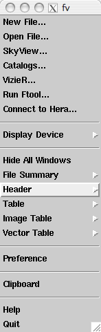\n",
138 | "\n",
139 | "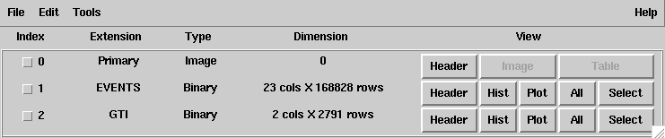\n",
140 | "\n",
141 | "This will bring up two windows:\n",
142 | "- the *fv* menu window \n",
143 | "- summary information about the file you are looking at \n",
144 | "\n",
145 | "\n",
146 | "For the purposes of the tutorial, we will only be using the summary window, but feel free to explore the options in the main menu window as well.\n",
147 | "\n",
148 | "The summary window shows:\n",
149 | "\n",
150 | "1. There is an empty primary array and two FITS extensions (`EVENTS`, the events table & `GTI`, the table of good time intervals). This is the normal file structure for a LAT events file. (If you don't see this structure, there is something wrong with your file.)\n",
151 | "\n",
152 | "2. There are 168828 events in the filtered 3C279 file (the number of rows in the EVENTS extension), and 22 pieces of information (the number of columns) for each event.\n",
153 | "\n",
154 | "3. There are 2791 GTI entries.\n",
155 | "\n",
156 | "From this window, data can be viewed in different ways:\n",
157 | "\n",
158 | "* For each extension, the FITS header can be examined for keywords and their values.\n",
159 | "\n",
160 | "* Histograms and plots can be made of the data in the EVENTS and GTI extensions.\n",
161 | "\n",
162 | "* Data in the EVENTS or GTI extensions can also be viewed directly.\n",
163 | "\n",
164 | "Let's look at each of these in turn."
165 | ]
166 | },
167 | {
168 | "cell_type": "markdown",
169 | "metadata": {},
170 | "source": [
171 | "### Viewing an Extension Header\n",
172 | "\n",
173 | "Click on the `Header` button for the EVENTS extension; a new window listing all the header keywords and their values for this extension will be displayed. Notice that the same information is presented that was shown in the summary window; namely that: the data is a binary table (XTENSION='BINTABLE'); there are 123857 entries (NAXIS2=123857); and there are 22 data values for each event (TFIELDS=22).\n",
174 | "\n",
175 | "In addition, there is information about the size (in bytes) of each row and the descriptions of each of the data fields contained in the table.\n",
176 | "\n",
177 | "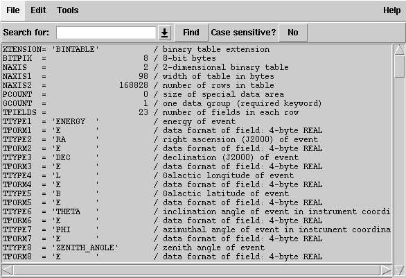\n",
178 | "\n",
179 | "As you scroll down, you will find some other useful information:\n",
180 | "\n",
181 | "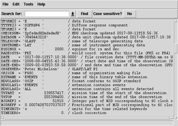\n",
182 | "\n",
183 | "Important keywords in the HEADER include:\n",
184 | "* **DATE** - The date the file was created.\n",
185 | "* **DATE-OBS** - The starting time, in UTC, of the data in the file.\n",
186 | "* **DATE-END** - The ending time, in UTC, of the data in the file.\n",
187 | "* **TSTART** - The equivalant of **DATE-OBS** but in Mission Elapsed Time (MET). Note: MET is the time system used in the event file to time tag all events.\n",
188 | "* **TSTOP** - The equivalant of **DATE-END** in MET.\n",
189 | "* **MJDREFI** - The integer Modified Julian Date (MJD) of the zero point for MET. This corresponds to midnight, Jan. 1st, 2001 for FERMI\n",
190 | "* **MJDREFF** - the fractional value of the reference Modified Julian Date, = 0.0007428703770377037\n",
191 | "\n",
192 | "Finally, as you continue scrolling to the bottom of the header, you will see:\n",
193 | "\n",
194 | "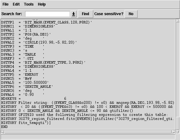\n",
195 | "\n",
196 | "This part of the header contains information about the data cuts that were used to extract the data. These are contained in the various DSS keywords. For a full description of the meaning of these values see the [DSS keyword page](https://fermi.gsfc.nasa.gov/ssc/data/analysis/scitools/dss_keywords.html). In this file the DSVAL1 keyword tells us which kind of event class has been used, the DSVAL2 keyword tells us that the data was extracted in a circular region, 20 degrees in radius, centered on RA=193.98 and DEC=-5.82. The DSVAL3 keyword shows us that the valid time range is defined by the GTIs. The DSVAL4 keywords shows the selected energy range in MeV, and DSVAL5 indicates that a zenith angle cut has been defined."
197 | ]
198 | },
199 | {
200 | "cell_type": "markdown",
201 | "metadata": {},
202 | "source": [
203 | "### Making a Counts Map"
204 | ]
205 | },
206 | {
207 | "cell_type": "markdown",
208 | "metadata": {},
209 | "source": [
210 | "*fv* can also be used to make a quick counts map to see what the region you extracted looks like. To do this:\n",
211 | "\n",
212 | "1. In the summary window for the FITS file, click on the **Hist** button for the EVENTS extension. A Histogram window will open.\n",
213 | ">**Note**: We use the histogram option rather than the plot option, as that would produce a scatter plot.\n",
214 | "\n",
215 | "2. From the X column's drop down menu in the column name field, select **RA**.\n",
216 | "fv will automatically fill in the TLMin, TLMax, Data Min and Data Max fields based on the header keywords and data values for that column. It will also make guesses for the values of the Min, Max and Bin Size fields.\n",
217 | "\n",
218 | "3. From the Y column's drop down menu in the column name field, select **DEC** from the list of columns.\n",
219 | "\n",
220 | "4. Select the limits on each of the coordinates in the Min and Max boxes.\n",
221 | "In this example, we've selected the limits to be just larger than the values in the Data Min and Data Max field for each column.\n",
222 | "\n",
223 | "5. Set the bin size for each column (in the units of the respective column; in this case we used 0.1 degrees).\n",
224 | "\n",
225 | "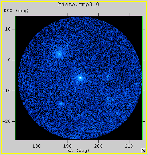\n",
226 | "\n",
227 | "For this map, we've selected 0.1 degree bins."
228 | ]
229 | },
230 | {
231 | "cell_type": "markdown",
232 | "metadata": {},
233 | "source": [
234 | "6. You can also select a data column from the FITS file to use as a weight if you desire.\n",
235 | "For example, if you wanted to make an approximated flux map, you could select the ENERGY column in the Weight field and the counts would be weighted by their energy.\n",
236 | "\n",
237 | "\n",
238 | "7. Click on the `Make` button to generate the map.\n",
239 | "\n",
240 | " This will create the plot in a new window and keep the histogram window open in case you want to make changes and create a different image. The \"Make/Close\" button will create the image and close the histogram window.\n",
241 | "\n",
242 | " *fv* also allows you to adjust the color and scale, just as you can in *ds9*. However, it has a different selection of color maps.\n",
243 | "\n",
244 | " As in *ds9*, the default is gray scale. The image at right was displayed with the cold color map, selected by clicking on the \"Colors\" menu item, then selecting: \"Continuous\" submenu --> \"cold\" check box."
245 | ]
246 | },
247 | {
248 | "cell_type": "markdown",
249 | "metadata": {},
250 | "source": [
251 | "# 2. Binning the Data\n",
252 | "\n",
253 | "While *ds9* and *fv* can be used to make quick look plots when exploring the data, they don't automatically do all the things you would like when making data files for analysis. For this, you will need to use the *Fermi*-specific [gtbin](https://fermi.gsfc.nasa.gov/ssc/data/analysis/scitools/help/gtbin.txt) tool to manipulate the data."
254 | ]
255 | },
256 | {
257 | "cell_type": "markdown",
258 | "metadata": {},
259 | "source": [
260 | "You can use [gtbin](https://fermi.gsfc.nasa.gov/ssc/data/analysis/scitools/help/gtbin.txt) to bin photon data into the following representations:\n",
261 | "\n",
262 | "* Images (maps)\n",
263 | "* Light curves\n",
264 | "* Energy spectra (PHA files)\n",
265 | "\n",
266 | "This has the advantage of creating the files in exactly the format needed by the other science tools as well as by other analysis tools such as [XSPEC](http://heasarc.gsfc.nasa.gov/docs/xanadu/xspec/), and of adding correct WCS keywords to the images so that the coordinate systems are properly displayed when using image viewers (such as *ds9* and *fv*) that can correctly interpret the WCS keywords."
267 | ]
268 | },
269 | {
270 | "cell_type": "markdown",
271 | "metadata": {},
272 | "source": [
273 | "In this section we will use the [3C279_region_filtered_gti.fits](https://fermi.gsfc.nasa.gov/ssc/data/analysis/scitools/data/exploreLATData/3C279_region_filtered_gti.fits) file to make images and will look at the results with *ds9*. In the [Explore LAT Data (for Burst)](https://fermi.gsfc.nasa.gov/ssc/data/analysis/scitools/explore_latdata_burst.html) section we will show how to use [gtbin](https://fermi.gsfc.nasa.gov/ssc/data/analysis/scitools/help/gtbin.txt) to produce a light curve.\n",
274 | "\n",
275 | "Just as with *fv* and *ds9*, *gtbin* can be used to make counts maps out of the extracted data.\n",
276 | "\n",
277 | "The main advantage of using [gtbin](https://fermi.gsfc.nasa.gov/ssc/data/analysis/scitools/help/gtbin.txt) is that it adds the proper header keywords so that the coordinate system is properly displayed as you move around the image.\n",
278 | "\n",
279 | "Here, we'll make the same image of the anti-center region that we make with *fv* and *ds9*, but this time we'll use the [gtbin](https://fermi.gsfc.nasa.gov/ssc/data/analysis/scitools/help/gtbin.txt) tool to make the image."
280 | ]
281 | },
282 | {
283 | "cell_type": "markdown",
284 | "metadata": {},
285 | "source": [
286 | "[gtbin](https://fermi.gsfc.nasa.gov/ssc/data/analysis/scitools/help/gtbin.txt) is invoked on the command line with or without the name of the file you want to process. If no file name is given, [gtbin](https://fermi.gsfc.nasa.gov/ssc/data/analysis/scitools/help/gtbin.txt) will prompt for it."
287 | ]
288 | },
289 | {
290 | "cell_type": "code",
291 | "execution_count": null,
292 | "metadata": {},
293 | "outputs": [],
294 | "source": [
295 | "%%bash\n",
296 | "gtbin\n",
297 | " CMAP\n",
298 | " ./data/3C279_region_filtered_gti.fits\n",
299 | " ./data/3C279_region_cmap.fits\n",
300 | " NONE\n",
301 | " 400\n",
302 | " 400\n",
303 | " 0.1\n",
304 | " CEL\n",
305 | " 193.98\n",
306 | " -5.82\n",
307 | " 0\n",
308 | " AIT\n",
309 | "\n",
310 | "#### Parameters:\n",
311 | "# Type of output file (CCUBE|CMAP|LC|PHA1|PHA2)\n",
312 | "# Event data file name\n",
313 | "# Output file name\n",
314 | "# Spacecraft data file name [NONE is valid]\n",
315 | "# Size of the X axis in pixels\n",
316 | "# Size of the Y axis in pixels\n",
317 | "# Image scale (in degrees/pixel)\n",
318 | "# Coordinate system (CEL - celestial, GAL -galactic) (CEL|GAL)\n",
319 | "# First coordinate of image center in degrees (RA or galactic l)\n",
320 | "# Second coordinate of image center in degrees (DEC or galactic b)\n",
321 | "# Rotation angle of image axis, in degrees\n",
322 | "# Projection method e.g. AIT|ARC|CAR|GLS|MER|NCP|SIN|STG|TAN\n",
323 | "#\n",
324 | "# For strange reasons, gtbin cannot be run with the ! magic; instead, we use the %%bash magic."
325 | ]
326 | },
327 | {
328 | "cell_type": "markdown",
329 | "metadata": {},
330 | "source": [
331 | "There are many different possible projection types. For a small region of the sky, the difference between projections is small, but is more significant for larger regions of the sky."
332 | ]
333 | },
334 | {
335 | "cell_type": "markdown",
336 | "metadata": {},
337 | "source": [
338 | "In this case, we want a counts map, so we:\n",
339 | "1. Select `CMAP`.\n",
340 | "\n",
341 | " The CCUBE (counts cube) option produces a set of count maps over several energy bins.\n",
342 | " \n",
343 | " \n",
344 | "2. Provide an **output file name**.\n",
345 | "3. Specify `NONE` for the spacecraft file as it is not needed for the counts map.\n",
346 | "4. Input **image size and scale** in pixels and degrees/pixel.\n",
347 | "\n",
348 | " **Note**: We select a 400x400 pixel image with 0.1 degree pixels in order to create an image that contains all the extracted data.\n",
349 | " \n",
350 | " \n",
351 | "5. Enter the **coordinate system**, either celestial (CEL) or galactic (GAL), to be used in generating the image. The coordinates for the image center (next bullet) must be in the indicated coordinate system.\n",
352 | "6. Enter the **coordinates** for the center of the image, which here correspond to the position of 3C 279.\n",
353 | "7. Enter the **rotation angle (0)**.\n",
354 | "8. Enter the projection method for the image. See Calabretta & Greisen 2002, A&A, 395, 1077 for definitions of these projections. An AITOFF projection is selected.\n",
355 | "\n",
356 | "Here is the output [counts map file](https://fermi.gsfc.nasa.gov/ssc/data/analysis/scitools/data/exploreLATData/3C279_region_cmap.fits) to use for comparison, displayed in *ds9*.\n",
357 | "\n",
358 | "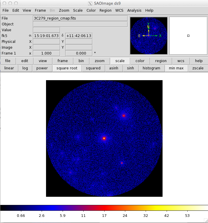\n",
359 | "\n",
360 | "Compare this result to the images made with *fv* and *ds9* and you will notice that the image is flipped along the y-axis.\n",
361 | "\n",
362 | "This is because the coordinate system keywords have been properly added to the image header and the Right Ascension (RA) coordinate actual increases right to left and not left to right.\n",
363 | "\n",
364 | "Moving the cursor over the image now shows the RA and Dec of the cursor position in the FK5 fields in the top left section of the display.\n",
365 | "\n",
366 | "If you want to look at coordinates in another system, such as galactic coordinates, you can make the change by first selecting the '**WCS**' button (on the right in the top row of buttons), and then the appropriate coordinate system from the choices that appear in the second row of buttons (FK4, FK5, IRCS, Galactic or Ecliptic)."
367 | ]
368 | },
369 | {
370 | "cell_type": "markdown",
371 | "metadata": {},
372 | "source": [
373 | "# 3. Examining Exposure Maps\n",
374 | "\n",
375 | "In this section, we explore ways of generating and looking at exposure maps. If you have not yet run [gtmktime](https://fermi.gsfc.nasa.gov/ssc/data/analysis/scitools/help/gtmktime.txt) on the data file you are examining, this analysis will likely yield incorrect results. It is advisable to prepare your data file properly by following the [Data Preparation](https://fermi.gsfc.nasa.gov/ssc/data/analysis/scitools/data_preparation.html) tutorial before looking in detail at the [livetime and exposure](https://fermi.gsfc.nasa.gov/ssc/data/analysis/documentation/Cicerone/Cicerone_Data_Exploration/livetime_and_exposure.html).\n",
376 | "\n",
377 | "Generally, to look at the exposure you must:\n",
378 | "\n",
379 | "1. Make an livetime cube from the spacecraft data file using **gtltcube**.\n",
380 | "2. As necessary, merge multiple livetime cubes covering different time ranges.\n",
381 | "3. Create the exposure map using the **gtexpmap** tool.\n",
382 | "4. Examine the map using *ds9*."
383 | ]
384 | },
385 | {
386 | "cell_type": "markdown",
387 | "metadata": {},
388 | "source": [
389 | "### Calculate the Livetime\n",
390 | "\n",
391 | "In order to determine the exposure for your source, you need to understand how much time the LAT has observed any given position on the sky at any given inclination angle.\n",
392 | "\n",
393 | "[gtltcube](https://fermi.gsfc.nasa.gov/ssc/data/analysis/scitools/help/gtltcube.txt) calculates this 'livetime cube' for the entire sky for the time range covered by the spacecraft file.\n",
394 | "\n",
395 | "To do this, you will need to make the livetime cube from the spacecraft (pointing and livetime history) file, using the [gtltcube](https://fermi.gsfc.nasa.gov/ssc/data/analysis/scitools/help/gtltcube.txt) tool."
396 | ]
397 | },
398 | {
399 | "cell_type": "code",
400 | "execution_count": null,
401 | "metadata": {},
402 | "outputs": [],
403 | "source": [
404 | "!gtltcube \\\n",
405 | " evfile =./data/3C279_region_filtered_gti.fits \\\n",
406 | " scfile = ./data/spacecraft.fits \\\n",
407 | " outfile = ./data/3C279_region_ltcube.fits \\\n",
408 | " dcostheta = 0.025 \\\n",
409 | " binsz = 1\n",
410 | "\n",
411 | "#### gtltcube Parameters:\n",
412 | "# Event data file\n",
413 | "# Spacecraft data file\n",
414 | "# Output file\n",
415 | "# Step size in cos(theta) (0.:1.)\n",
416 | "# Pixel size (degrees)\n",
417 | "#\n",
418 | "# May take a while to finish"
419 | ]
420 | },
421 | {
422 | "cell_type": "markdown",
423 | "metadata": {},
424 | "source": [
425 | "**gtltcube** may take some time to finish."
426 | ]
427 | },
428 | {
429 | "cell_type": "markdown",
430 | "metadata": {},
431 | "source": [
432 | "As you can see below in the image of the *fv* summary window below, the details recorded in the livetime cube file are multi-dimensional and difficult to visualize. For that, we will need an exposure map.\n",
433 | "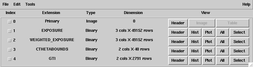\n",
434 | "\n",
435 | "### Combining _multiple_ livetime cubes\n",
436 | "\n",
437 | "In some cases, you will have multiple livetime cubes covering different periods of time that you wish to combine in order to examine the exposure over the entire time range.\n",
438 | "\n",
439 | "One example would be the researcher who generates weekly flux datapoints for light curves, and has the need to analyze the source significance over a larger time period. In this case, it is much less CPU-intensive to combine previously generated livetime cubes before calculating the exposure map, than to start the livetime cube generation from scratch.\n",
440 | "\n",
441 | "To combine multiple livetime cubes into a single cube use the [gtltsum](https://fermi.gsfc.nasa.gov/ssc/data/analysis/scitools/help/gtltsum.txt) tool."
442 | ]
443 | },
444 | {
445 | "cell_type": "markdown",
446 | "metadata": {},
447 | "source": [
448 | "**Note**: [gtltsum](https://fermi.gsfc.nasa.gov/ssc/data/analysis/scitools/help/gtltsum.txt) is quick, but it does have a few limitations, including:\n",
449 | "* It will only add two cubes at a time. If you have more than one cube to add, you must do them sequentially.\n",
450 | "\n",
451 | "* It does not allow you to append to or overwrite an existing livetime cube file.\n",
452 | "\n",
453 | " For example: if you wanted to add four cubes (c1, c2, c3 and c4), you cannot add c1 and c2 to get cube_a, then add cube_a and c3 and save the result as cube_a; you must use different file names for the output livetime cubes at each step.\n",
454 | "\n",
455 | "\n",
456 | "* The calculation parameters that were used to generate the livetime cubes (step size and pixel size) must be identical between the livetime cubes."
457 | ]
458 | },
459 | {
460 | "cell_type": "markdown",
461 | "metadata": {},
462 | "source": [
463 | "Here is an example of adding two livetime cubes from the first and second halves of the six months of 3C 279 data using **gtltsum** (where the midpoint was 247477908 MET):"
464 | ]
465 | },
466 | {
467 | "cell_type": "code",
468 | "execution_count": null,
469 | "metadata": {},
470 | "outputs": [],
471 | "source": [
472 | "!wget \"https://fermi.gsfc.nasa.gov/ssc/data/analysis/scitools/data/exploreLATData/3C279_region_first_ltcube.fits\"\n",
473 | "!wget \"https://fermi.gsfc.nasa.gov/ssc/data/analysis/scitools/data/exploreLATData/3C279_region_second_ltcube.fits\""
474 | ]
475 | },
476 | {
477 | "cell_type": "code",
478 | "execution_count": null,
479 | "metadata": {},
480 | "outputs": [],
481 | "source": [
482 | "!mv *cube.fits ./data"
483 | ]
484 | },
485 | {
486 | "cell_type": "code",
487 | "execution_count": null,
488 | "metadata": {},
489 | "outputs": [],
490 | "source": [
491 | "!ls ./data"
492 | ]
493 | },
494 | {
495 | "cell_type": "code",
496 | "execution_count": null,
497 | "metadata": {},
498 | "outputs": [],
499 | "source": [
500 | "!gtltsum \\\n",
501 | " infile1 = ./data/3C279_region_first_ltcube.fits \\\n",
502 | " infile2 = ./data/3C279_region_second_ltcube.fits \\\n",
503 | " outfile = ./data/3C279_region_summed_ltcube.fits\n",
504 | "\n",
505 | "#### Parameters:\n",
506 | "# Livetime cube 1 or list of files\n",
507 | "# Livetime cube 2\n",
508 | "# Output file"
509 | ]
510 | },
511 | {
512 | "cell_type": "markdown",
513 | "metadata": {},
514 | "source": [
515 | "### Generate an Exposure Map or Cube\n",
516 | "\n",
517 | "Once you have a livetime cube for the entire dataset, you need to calculate the exposure for your dataset. This can be in the form of an exposure **map** or an exposure **cube**.\n",
518 | "\n",
519 | "* Exposure **maps** are mono-energetic, and each plane represents the exposure at the midpoint of the energy band, not integrated over the band's energy range. Exposure maps are used for **unbinned** analysis methods. You will specify the number of energy bands when you run the [gtexpmap](https://fermi.gsfc.nasa.gov/ssc/data/analysis/scitools/help/gtexpmap.txt) tool.\n",
520 | "\n",
521 | "* Exposure **cubes** are used for **binned** analysis methods. The binning in both position and energy must match the binning of the input data file, which will be a counts cube. When you run the [gtexpcube2](https://fermi.gsfc.nasa.gov/ssc/data/analysis/scitools/help/gtexpcube2.txt) tool, you must be sure the binning matches.\n",
522 | "\n",
523 | "For simplicity, we will generate an exposure map by running the [gtexpmap](https://fermi.gsfc.nasa.gov/ssc/data/analysis/scitools/help/gtexpmap.txt) tool on the event file."
524 | ]
525 | },
526 | {
527 | "cell_type": "markdown",
528 | "metadata": {},
529 | "source": [
530 | "[**gtexpmap**](https://fermi.gsfc.nasa.gov/ssc/data/analysis/scitools/help/gtexpmap.txt) allows you to control the exposure map parameters, including:\n",
531 | "\n",
532 | "* Map center, size, and scale\n",
533 | "* Projection type (selection includes Aitoff, Cartesian, Mercator, Tangential, etc.; default is Aitoff)\n",
534 | "* Energy range\n",
535 | "* Number of energy bins\n",
536 | "\n",
537 | "The following example shows input and output for generating an exposure map for the region surrounding 3C 279."
538 | ]
539 | },
540 | {
541 | "cell_type": "code",
542 | "execution_count": null,
543 | "metadata": {},
544 | "outputs": [],
545 | "source": [
546 | "!gtexpmap \\\n",
547 | " evfile = ./data/3C279_region_filtered_gti.fits \\\n",
548 | " scfile = ./data/spacecraft.fits \\\n",
549 | " expcube = ./data/3C279_region_summed_ltcube.fits \\\n",
550 | " outfile = ./data/3C279_exposure_map.fits \\\n",
551 | " irfs = P8R3_SOURCE_V2 \\\n",
552 | " srcrad = 30 \\\n",
553 | " nlong = 500 \\\n",
554 | " nlat = 500 \\\n",
555 | " nenergies = 30\n",
556 | "\n",
557 | "#### gtexpmap Parameters: ALSO SEE BELOW\n",
558 | "# Event data file\n",
559 | "# Spacecraft data file\n",
560 | "# Exposure hypercube file\n",
561 | "# Output file name\n",
562 | "# Response functions\n",
563 | "# Radius of the source region (in degrees)\n",
564 | "# Number of longitude points (2:1000)\n",
565 | "# Number of latitude points (2:1000)\n",
566 | "# Number of energies (2:100)\n",
567 | "\n",
568 | "# This will generate an exposure map on six months of data.\n",
569 | "# This may take a long time.\n",
570 | "# Below you will find a wget command to get the resulting file."
571 | ]
572 | },
573 | {
574 | "cell_type": "markdown",
575 | "metadata": {},
576 | "source": [
577 | "**As six months is far too much data for an unbinned analysis, this computation will take a long time. Skip past this section to find a copy of the output file.**\n",
578 | "\n",
579 | "Running **gtexpmap** in the command line will prompt you to enter the following:\n",
580 | "\n",
581 | "* Name of an events file to determine the energy range to use.\n",
582 | "* Name of the exposure cube file to use.\n",
583 | "* Name of the output file and the instrument response function to use.\n",
584 | " * For more discussion on the proper instrument response function (IRF) to use in your data analysis, see the overview discussion in the [Cicerone](https://fermi.gsfc.nasa.gov/ssc/data/analysis/documentation/Cicerone/Cicerone_LAT_IRFs/IRF_overview.html), as well as the current [recommended data selection](https://fermi.gsfc.nasa.gov/ssc/data/analysis/documentation/Cicerone/Cicerone_Data_Exploration/Data_preparation.html) information from the LAT team. The [LAT data caveats](https://fermi.gsfc.nasa.gov/ssc/data/analysis/LAT_caveats.html) are also important to review before starting LAT analysis.\n",
585 | "\n",
586 | "The next set of parameters specify the size, scale, and position of the map to generate.\n",
587 | "\n",
588 | "* The radius of the 'source region'\n",
589 | " * The source region is different than the region of interest (ROI). This is the region that you will model when fitting your data. As every region of the sky that contains sources will also have adjacent regions containing sources, it is advisable to model an area larger than that covered by your dataset. Here we have increased the source region by an additional 10°, which is the minimum needed for an actual analysis. Be aware of what sources may be near your region, and model them if appropriate (especially if they are very bright in gamma rays).\n",
590 | "* Number of longitude and latitude points\n",
591 | "* Number of energy bins that will have maps created\n",
592 | " * This number can be small (∼5) for sources with flat spectra in the LAT regime. However, for sources like pulsars that vary in flux significantly over the LAT energy range, a larger number of energies is recommended, typically 10 per decade in energy."
593 | ]
594 | },
595 | {
596 | "cell_type": "code",
597 | "execution_count": null,
598 | "metadata": {},
599 | "outputs": [],
600 | "source": [
601 | "# Get the output exposure map\n",
602 | "!wget \"https://fermi.gsfc.nasa.gov/ssc/data/analysis/scitools/data/exploreLATData/3C279_exposure_map.fits\""
603 | ]
604 | },
605 | {
606 | "cell_type": "code",
607 | "execution_count": null,
608 | "metadata": {},
609 | "outputs": [],
610 | "source": [
611 | "!mv 3C279_exposure_map.fits ./data/3C279_exposure_map.fits"
612 | ]
613 | },
614 | {
615 | "cell_type": "code",
616 | "execution_count": null,
617 | "metadata": {},
618 | "outputs": [],
619 | "source": [
620 | "!ls ./data"
621 | ]
622 | },
623 | {
624 | "cell_type": "markdown",
625 | "metadata": {},
626 | "source": [
627 | "Once the file has been generated, it can be viewed with *ds9*. When you open the file in *ds9*, a \"Data Cube\" window will appear, allowing you to select between the various maps generated."
628 | ]
629 | },
630 | {
631 | "cell_type": "code",
632 | "execution_count": null,
633 | "metadata": {},
634 | "outputs": [],
635 | "source": [
636 | "!ds9 ./data/3C279_exposure_map.fits"
637 | ]
638 | },
639 | {
640 | "cell_type": "markdown",
641 | "metadata": {
642 | "pycharm": {
643 | "name": "#%% md\n"
644 | }
645 | },
646 | "source": [
647 | "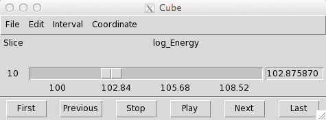\n",
648 | "\n",
649 | "\n",
650 | "Below are four of the 30 layers in the map, scaled by `log(Energy)`, and extracted from *ds9*.\n",
651 | "\n",
652 | "| First Layer | Fourth Layer |\n",
653 | "| --- | --- |\n",
654 | "| |  |\n",
655 | "\n",
656 | "| Tenth Layer | Last Layer |\n",
657 | "| --- | --- |\n",
658 | "| 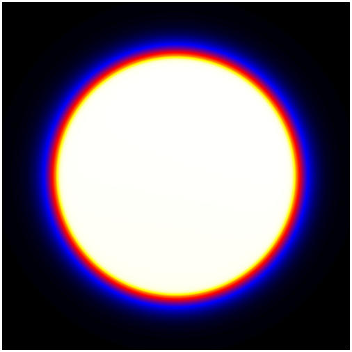 | 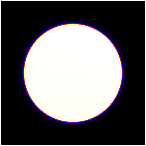 |\n",
659 | "\n",
660 | "\n",
661 | "As you can see, the exposure changes as you go to higher energies. This is due to two effects:\n",
662 | "\n",
663 | "1. The [PSF](https://fermi.gsfc.nasa.gov/ssc/data/analysis/documentation/Cicerone/Cicerone_LAT_IRFs/IRF_PSF.html) is broader at lower energies, making the wings of the exposure expand well outside the region of interest. This is why it is necessary to add at least 10 degrees to your ROI. In this case, you can see that even 10 degrees has not fully captured the wings of the PSF at low energies.\n",
664 | "\n",
665 | "\n",
666 | "2. The [effective area](https://fermi.gsfc.nasa.gov/ssc/data/analysis/documentation/Cicerone/Cicerone_LAT_IRFs/IRF_EA.html) of the LAT changes at higher energies.\n",
667 | "\n",
668 | "Both of these effects are quantified on the [LAT performance page](http://www.slac.stanford.edu/exp/glast/groups/canda/lat_Performance.htm)."
669 | ]
670 | }
671 | ],
672 | "metadata": {
673 | "kernelspec": {
674 | "display_name": "Python 3",
675 | "language": "python",
676 | "name": "python3"
677 | },
678 | "language_info": {
679 | "codemirror_mode": {
680 | "name": "ipython",
681 | "version": 3
682 | },
683 | "file_extension": ".py",
684 | "mimetype": "text/x-python",
685 | "name": "python",
686 | "nbconvert_exporter": "python",
687 | "pygments_lexer": "ipython3",
688 | "version": "3.7.9"
689 | },
690 | "nav_menu": {},
691 | "pycharm": {
692 | "stem_cell": {
693 | "cell_type": "raw",
694 | "metadata": {
695 | "collapsed": false
696 | },
697 | "source": []
698 | }
699 | },
700 | "toc": {
701 | "navigate_menu": true,
702 | "number_sections": true,
703 | "sideBar": true,
704 | "threshold": 6,
705 | "toc_cell": false,
706 | "toc_section_display": "block",
707 | "toc_window_display": false
708 | }
709 | },
710 | "nbformat": 4,
711 | "nbformat_minor": 2
712 | }
713 |
--------------------------------------------------------------------------------
/DataSelection/4.ExploreLATDataBurst/explore_latdata_burst.ipynb:
--------------------------------------------------------------------------------
1 | {
2 | "cells": [
3 | {
4 | "cell_type": "markdown",
5 | "metadata": {},
6 | "source": [
7 | "# Explore LAT Data (for Burst)\n",
8 | "\n",
9 | "In this example, we will examine the LAT data for a gamma-ray burst based on the time and position derived from a GBM trigger."
10 | ]
11 | },
12 | {
13 | "cell_type": "markdown",
14 | "metadata": {},
15 | "source": [
16 | "# Prerequisites\n",
17 | "\n",
18 | "It is assumed that:\n",
19 | "\n",
20 | "* You are in your working directory.\n",
21 | "* The GBM reported a burst via a [GCN circular]() with the following information:\n",
22 | " * Name = GRB 080916C\n",
23 | " * RA = 121.8\n",
24 | " * Dec = -61.3\n",
25 | " * TStart = 243216766 s (Mission Elapsed Time)\n",
26 | " * T90 = 66 s"
27 | ]
28 | },
29 | {
30 | "cell_type": "markdown",
31 | "metadata": {},
32 | "source": [
33 | "# Steps\n",
34 | "\n",
35 | "The analysis steps are:\n",
36 | "\n",
37 | "1. Extract the Data\n",
38 | "2. Data Selections\n",
39 | "3. Bin the Data\n",
40 | "4. Look at the Data"
41 | ]
42 | },
43 | {
44 | "cell_type": "markdown",
45 | "metadata": {},
46 | "source": [
47 | "## 1. Extract the Data\n",
48 | "\n",
49 | "Generally, one should refer to [Extract LAT data](https://fermi.gsfc.nasa.gov/ssc/data/p6v11/analysis/scitools/extract_latdata.html) tutorial and use the time and spatial information from some source (here, a GCN notice) to make the appropiate extraction cuts from the [LAT data server](http://fermi.gsfc.nasa.gov/cgi-bin/ssc/LAT/LATDataQuery.cgi)."
50 | ]
51 | },
52 | {
53 | "cell_type": "markdown",
54 | "metadata": {},
55 | "source": [
56 | "We use the following parameters to extract the data for an ROI of 20 degrees from 500s before to 1500 seconds after the trigger time:\n",
57 | "\n",
58 | "* Search Center (RA,Dec)\t=\t(121.8,-61.3)\n",
59 | "* Radius\t=\t20 degrees\n",
60 | "* Start Time (MET)\t=\t243216266 seconds (2008-09-16T00:04:26)\n",
61 | "* Stop Time (MET)\t=\t243218266 seconds (2008-09-16T00:37:46)\n",
62 | "* Minimum Energy\t=\t20 MeV\n",
63 | "* Maximum Energy\t=\t300000 MeV\n",
64 | "\n",
65 | "Note that for analyses that require the diffuse background, the standard model starts at 60 MeV."
66 | ]
67 | },
68 | {
69 | "cell_type": "code",
70 | "execution_count": null,
71 | "metadata": {},
72 | "outputs": [],
73 | "source": [
74 | "!wget https://fermi.gsfc.nasa.gov/ssc/data/analysis/scitools/data/exploreLATDataGRB/LAT_explore_GRB.tgz"
75 | ]
76 | },
77 | {
78 | "cell_type": "code",
79 | "execution_count": null,
80 | "metadata": {},
81 | "outputs": [],
82 | "source": [
83 | "!tar xvzf LAT_explore_GRB.tgz"
84 | ]
85 | },
86 | {
87 | "cell_type": "code",
88 | "execution_count": null,
89 | "metadata": {},
90 | "outputs": [],
91 | "source": [
92 | "!mkdir data\n",
93 | "!mv *.fits ./data"
94 | ]
95 | },
96 | {
97 | "cell_type": "code",
98 | "execution_count": null,
99 | "metadata": {},
100 | "outputs": [],
101 | "source": [
102 | "!ls ./data"
103 | ]
104 | },
105 | {
106 | "cell_type": "markdown",
107 | "metadata": {},
108 | "source": [
109 | "This will extract the data files used in this tutorial into the `data` directory."
110 | ]
111 | },
112 | {
113 | "cell_type": "markdown",
114 | "metadata": {},
115 | "source": [
116 | "## Data Selections\n",
117 | "\n",
118 | "NOTE: For information on the recommended selections for burst analysis of LAT data, you should refer to the [Cicerone](http://fermi.gsfc.nasa.gov/ssc/data/p6v11/analysis/documentation/Cicerone/Cicerone_Data_Exploration/Data_preparation.html).\n",
119 | "\n",
120 | "To map the region of the burst, you should select a large spatial region from within a short time range bracketing the burst. For the lightcurve on the other hand, its best to select you want a small region around the burst from within a long time range. Therefore, you will need to make two different data selections.\n",
121 | "\n",
122 | "In both cases, we will use the loosest event class cut (to include all class events). This works because rapid, bright events like GRBs overwhelm the background rates for the short period of the flare."
123 | ]
124 | },
125 | {
126 | "cell_type": "markdown",
127 | "metadata": {},
128 | "source": [
129 | "Here, we use [gtselect](https://fermi.gsfc.nasa.gov/ssc/data/p6v11/analysis/scitools/help/gtselect.txt) to extract the region for the spatial mapping:"
130 | ]
131 | },
132 | {
133 | "cell_type": "code",
134 | "execution_count": null,
135 | "metadata": {},
136 | "outputs": [],
137 | "source": [
138 | "%%bash\n",
139 | "gtselect evclass=128\n",
140 | " ./data/grb_events.fits\n",
141 | " ./data/GRB081916C_map_events.fits\n",
142 | " 121.8\n",
143 | " -61.3\n",
144 | " 20\n",
145 | " 243216666\n",
146 | " 243216966\n",
147 | " 100\n",
148 | " 300000\n",
149 | " 180"
150 | ]
151 | },
152 | {
153 | "cell_type": "markdown",
154 | "metadata": {},
155 | "source": [
156 | "**Notes**:\n",
157 | "* The input photon file is `grb_events.fits`, and the output file is `GRB081916C_map_events.fits`.\n",
158 | "* We selected a circular region with radius 20 degree around the burst location (the ROI here has to fall within that selected in the data server) from a 300s time period around the trigger.\n",
159 | "* We made an additional energy cut, selecting only photons between 100 MeV and 300 GeV. This removes the low-energy high-background events from the map."
160 | ]
161 | },
162 | {
163 | "cell_type": "markdown",
164 | "metadata": {},
165 | "source": [
166 | "**Run [gtselect](https://fermi.gsfc.nasa.gov/ssc/data/p6v11/analysis/scitools/help/gtselect.txt) again**, this time with a smaller region but a longer time range. (Note that _gtselect_ saves the values from the previous run and uses them as defaults for the next run.)"
167 | ]
168 | },
169 | {
170 | "cell_type": "code",
171 | "execution_count": null,
172 | "metadata": {},
173 | "outputs": [],
174 | "source": [
175 | "%%bash\n",
176 | "gtselect evclass=128\n",
177 | " ./data/grb_events.fits\n",
178 | " ./data/GRB081916C_lc_events.fits\n",
179 | " 121.8\n",
180 | " -61.3\n",
181 | " 10\n",
182 | " 243216266\n",
183 | " 243218266\n",
184 | " 30\n",
185 | " 300000\n",
186 | " 180"
187 | ]
188 | },
189 | {
190 | "cell_type": "markdown",
191 | "metadata": {},
192 | "source": [
193 | "**Notes**:\n",
194 | "\n",
195 | "* A new output file, with the extension `lc_events.fits` has been produced.\n",
196 | "* The search radius was reduced to 10 degrees.\n",
197 | "* The start to stop time range has been expanded.\n",
198 | "* The energy range has been expanded."
199 | ]
200 | },
201 | {
202 | "cell_type": "markdown",
203 | "metadata": {},
204 | "source": [
205 | "## Bin the Data\n",
206 | "\n",
207 | "Use [gtbin](https://fermi.gsfc.nasa.gov/ssc/data/p6v11/analysis/scitools/help/gtbin.txt) to bin the photon data into a map and a lightcurve.\n",
208 | "\n",
209 | "First, create the counts map:"
210 | ]
211 | },
212 | {
213 | "cell_type": "code",
214 | "execution_count": null,
215 | "metadata": {},
216 | "outputs": [],
217 | "source": [
218 | "%%bash\n",
219 | "gtbin\n",
220 | " CMAP\n",
221 | " ./data/GRB081916C_map_events.fits\n",
222 | " ./data/GRB081916C_counts_map.fits\n",
223 | " NONE\n",
224 | " 50\n",
225 | " 50\n",
226 | " 0.5\n",
227 | " CEL\n",
228 | " 121.8\n",
229 | " -61.3\n",
230 | " 0.\n",
231 | " AIT"
232 | ]
233 | },
234 | {
235 | "cell_type": "markdown",
236 | "metadata": {},
237 | "source": [
238 | "**Notes**:\n",
239 | " \n",
240 | "* Select _cmap_ (i.e., count map) as the output.\n",
241 | "* When we ran _gtselect_ we called the file from a large area `GRB081916C_map_events.fits`.\n",
242 | "* The counts map file will be called `GRB081916C_counts_map.fits`.\n",
243 | "* Although in _gtselect_ we selected a circular region with a 20 degree radius, we will form a counts map with 50 pixels on a side, and 1/2 degree square pixels.\n",
244 | "\n",
245 | "Now, we create the lightcurve. Once again, the previous inputs were saved and provided as defaults where appropriate."
246 | ]
247 | },
248 | {
249 | "cell_type": "code",
250 | "execution_count": null,
251 | "metadata": {},
252 | "outputs": [],
253 | "source": [
254 | "%%bash\n",
255 | "gtbin\n",
256 | " LC\n",
257 | " ./data/GRB081916C_lc_events.fits\n",
258 | " ./data/GRB081916C_light_curve.fits\n",
259 | " NONE\n",
260 | " LIN\n",
261 | " 243216266\n",
262 | " 243218266\n",
263 | " 10"
264 | ]
265 | },
266 | {
267 | "cell_type": "markdown",
268 | "metadata": {},
269 | "source": [
270 | "**Notes**:\n",
271 | "* We used **gtselect** to create `GRB081916C_lc_events.fits`, a photon list from a small region but using a long time range.\n",
272 | "\n",
273 | "\n",
274 | "* **gtbin** binned these photons and output the result into `GRB081916C_light_curve.fits`.\n",
275 | "\n",
276 | " There are a number of options for choosing the time bins. Here we have chosen linear bins with equal time widths of 10 seconds."
277 | ]
278 | },
279 | {
280 | "cell_type": "markdown",
281 | "metadata": {},
282 | "source": [
283 | "## Examine the Data\n",
284 | "\n",
285 | "We now have two FITS files with binned data: one with a lightcurve (`GRB081916C_light_curve.fits`), and a second with a counts map (`GRB081916C_counts_map.fits`).\n",
286 | "\n",
287 | "**Note**: Currently we do not have any Fermi specific graphics programs, but there are various tools available to plot FITS data files, such as [_fv_](http://heasarc.nasa.gov/ftools/fv/) and [_ds9_](http://hea-www.harvard.edu/RD/ds9/)."
288 | ]
289 | },
290 | {
291 | "cell_type": "markdown",
292 | "metadata": {},
293 | "source": [
294 | "To look at the counts map, we will use *fv*.\n",
295 | "\n",
296 | "1. First, start up *fv* in your terminal using:\n",
297 | " prompt> fv &\n",
298 | " (Or see the code cell below)\n",
299 | " \n",
300 | " \n",
301 | "2. Then open `GRB081916C_counts_map.fits`. Click on 'open file' to get the `File Dialog` GUI. Choose `GRB081916C_counts_map.fits`. A new GUI will open up with a table with two rows.\n",
302 | "\n",
303 | "\n",
304 | "3. FITS files consist of a series of extensions with data. Since the counts map is an image, it is stored in the primary extension (for historical reasons only images can be stored in the primary extension). Clicking on the 'Image' button in the first row results in:"
305 | ]
306 | },
307 | {
308 | "cell_type": "code",
309 | "execution_count": null,
310 | "metadata": {},
311 | "outputs": [],
312 | "source": [
313 | "!fv ./data/GRB081916C_counts_map.fits"
314 | ]
315 | },
316 | {
317 | "cell_type": "code",
318 | "execution_count": null,
319 | "metadata": {},
320 | "outputs": [],
321 | "source": [
322 | "from IPython.display import HTML"
323 | ]
324 | },
325 | {
326 | "cell_type": "code",
327 | "execution_count": null,
328 | "metadata": {},
329 | "outputs": [],
330 | "source": [
331 | "HTML(\"\")"
332 | ]
333 | },
334 | {
335 | "cell_type": "markdown",
336 | "metadata": {},
337 | "source": [
338 | "One readily observes that there are many pixels containing a few counts each near the burst location, and few pixels containing any counts away from the burst. It is also evident that the burst location is not centered in the counts map. This means the preliminary location sent out in the GCN was not quite the right location. This is not uncommon for automated transient localizations.\n",
339 | "\n",
340 | "Using *ds9* instead of *fv* allows us to find the location of the brightest pixel, and a better position for the burst."
341 | ]
342 | },
343 | {
344 | "cell_type": "code",
345 | "execution_count": null,
346 | "metadata": {},
347 | "outputs": [],
348 | "source": [
349 | "HTML(\"\")"
350 | ]
351 | },
352 | {
353 | "cell_type": "markdown",
354 | "metadata": {},
355 | "source": [
356 | "By simply mousing over that pixel, the RA and Dec of the likely burst location get displayed in the FK5 boxes (here, the new position is 119.5, -56.5). This is a quick method of localizing a burst, though not as accurate as fitting the data (described in the [Likelihood Tutorial](https://fermi.gsfc.nasa.gov/ssc/data/p6v11/analysis/scitools/likelihood_tutorial.html)).\n",
357 | "\n",
358 | "> **Note**: To change the *ds9* display for the mouseover from sexagesimal (the default) to degrees, go to the WCS menu and select \"Degrees\" in the bottom portion of the menu."
359 | ]
360 | },
361 | {
362 | "cell_type": "markdown",
363 | "metadata": {},
364 | "source": [
365 | "**To look at the lightcurve:**\n",
366 | "\n",
367 | "1. Open `GRB081916C_light_curve.fits` in *fv*.\n",
368 | "\n",
369 | " The lightcurve is in the RATE extension. Choose 'All' to view the content of that extension. The extension has 4 columns: TIME, TIMEDEL, COUNTS and ERROR.\n",
370 | " \n",
371 | " The time bins were created to have a width of 10 seconds, and therefore TIMEDEL is always 10.\n",
372 | " \n",
373 | "2. Now plot the COUNTS as a function of TIME. Select 'Plot' for the RATE extension. Click on 'Time' then on 'x'. Click on 'Counts' then on 'y'. Finally click on 'Plot'. The result is:"
374 | ]
375 | },
376 | {
377 | "cell_type": "code",
378 | "execution_count": null,
379 | "metadata": {},
380 | "outputs": [],
381 | "source": [
382 | "!fv ./data/GrB081916C_light_curve.fits"
383 | ]
384 | },
385 | {
386 | "cell_type": "code",
387 | "execution_count": null,
388 | "metadata": {},
389 | "outputs": [],
390 | "source": [
391 | "HTML(\"\")"
392 | ]
393 | },
394 | {
395 | "cell_type": "markdown",
396 | "metadata": {},
397 | "source": [
398 | ">**Note**: Except for the period of the burst, almost all bins have 0-5 counts. This demonstrates that there is very little background for LAT observations of gamma-ray bursts."
399 | ]
400 | }
401 | ],
402 | "metadata": {
403 | "kernelspec": {
404 | "display_name": "Python 3",
405 | "language": "python",
406 | "name": "python3"
407 | },
408 | "language_info": {
409 | "codemirror_mode": {
410 | "name": "ipython",
411 | "version": 3
412 | },
413 | "file_extension": ".py",
414 | "mimetype": "text/x-python",
415 | "name": "python",
416 | "nbconvert_exporter": "python",
417 | "pygments_lexer": "ipython3",
418 | "version": "3.7.9"
419 | }
420 | },
421 | "nbformat": 4,
422 | "nbformat_minor": 2
423 | }
424 |
--------------------------------------------------------------------------------
/DataSelection/5.UsingLATAllSkyWeekly/LAT_weekly_allsky.ipynb:
--------------------------------------------------------------------------------
1 | {
2 | "cells": [
3 | {
4 | "cell_type": "markdown",
5 | "metadata": {},
6 | "source": [
7 | "# Using Fermi-LAT All-sky Weekly Files\n",
8 | "\n",
9 | "Some types of data analyses lend themselves to the use of all-sky data files, rather than repeatedly downloading overlapping regions of sky for repeat analysis. Examples are:\n",
10 | "\n",
11 | "* Light curves and spectra for a large number of sources, whether galactic, extragalactic, or both\n",
12 | "* Characterization of large-scale diffuse emission\n",
13 | "* Analysis of moving sources, like the Sun\n",
14 | "* Searches for transient events (like GRBs) that have an isotropic distribution\n",
15 | "\n",
16 | "This analysis thread describes how to generate an all-sky data set for use in other types of analysis. We will then create an exposure-corrected all-sky image as an example of how to use the weekly files."
17 | ]
18 | },
19 | {
20 | "cell_type": "markdown",
21 | "metadata": {},
22 | "source": [
23 | "## Download the weekly LAT files\n",
24 | "\n",
25 | "The weekly LAT data files are available from the FSSC [FTP Server](https://heasarc.gsfc.nasa.gov/FTP/fermi/data/lat/). These files contain the LAT data acquired during each week of Fermi's science mission. (Mission weeks run Thursday through Wednesday, UTC time.) The file for the current mission week will also be listed, even though the week may not yet be complete.\n",
26 | "\n",
27 | "The current mission week file is regenerated by the FSSC after every data delivery from the LAT instrument team. This guarantees that the FTP Server and the LAT data server contain the same data, and both are up-to-date.\n",
28 | "\n",
29 | "You can download the LAT weekly files one at a time from the FTP site, or you can use `wget` to download a full set of files.\n",
30 | "\n",
31 | "Once you have the current set of files, you can use the same `wget` command (from the same directory) to download only the newest files. In the event that the LAT team reprocesses data for the full mission, the filenames will change, and `wget` will download a full set of the new, reprocessed, data.\n",
32 | "\n",
33 | ">**Note**: This may take a while."
34 | ]
35 | },
36 | {
37 | "cell_type": "code",
38 | "execution_count": null,
39 | "metadata": {},
40 | "outputs": [],
41 | "source": [
42 | "!wget -m -P . -nH --cut-dirs=4 -np -e robots=off https://heasarc.gsfc.nasa.gov/FTP/fermi/data/lat/weekly/photon/"
43 | ]
44 | },
45 | {
46 | "cell_type": "markdown",
47 | "metadata": {},
48 | "source": [
49 | "LAT data has been classified based on the quality of the event reconstruction. The classification can then be used to reduce background and improve performance by filtering out poorly reconstructed events.\n",
50 | "\n",
51 | "With the advent of Pass 8 data reconstruction, there are a myriad of various event classes that are tailored for specific types of analysis. The user should see the [Cicerone](https://fermi.gsfc.nasa.gov/ssc/data/analysis/documentation/Cicerone/Cicerone_Data_Exploration/Data_preparation.html) pages for a full description of the various event classes (and types) available in Pass 8.\n",
52 | "\n",
53 | "For most analyses, the user will be interested in `SOURCE` class photons (`evclass=128`). However, analyses that are intrinsically signal limited require very low background. For example, a user studying large scale, diffuse structures may be interested in using the `CLEAN` (`evclass=256`) or even `ULTRACLEAN` (`evclass=512`) classes.\n",
54 | "\n",
55 | "There are two types of weekly files available; photon files and extended files. The photon weekly files contain all the SOURCE class and are usable for most analyses. The extended files contain the same events as the photon files, but also contain additional reconstruction information about each photon that may be useful if you are trying to characterize the quality of a particular signal, such as for dark matter line searches.\n",
56 | "\n",
57 | ">**NOTE**: For analysis of short timescale events (for example, GRBs) where the flux of the event is much brighter than the accrued background, the user may be interested in using the `TRANSIENT010` (`evclass=64`) event class. If you are interested in investigating transient events within LAT data, you cannot use the weekly files, as they have been prefiltered to contain SOURCE class photons. There are no weekly files that contain the `TRANSIENT` class events.\n",
58 | ">\n",
59 | ">In order to generate an all-sky dataset of `TRANSIENT` class events, you will need to perform a grid of [data server](https://fermi.gsfc.nasa.gov/cgi-bin/ssc/LAT/LATDataQuery.cgi) queries with the maximum radius of 60 degrees. Once you have downloaded data from the full sky, you will need to combine the files and filter out duplicate events. We recommend using the [FTOOLS](https://heasarc.gsfc.nasa.gov/lheasoft/ftools/ftools_menu.html) suite to perform these tasks.\n",
60 | "\n",
61 | "Run this command to download the weekly extended files:"
62 | ]
63 | },
64 | {
65 | "cell_type": "code",
66 | "execution_count": null,
67 | "metadata": {},
68 | "outputs": [],
69 | "source": [
70 | "!wget -m -P . -nH --cut-dirs=4 -np -e robots=off https://heasarc.gsfc.nasa.gov/FTP/fermi/data/lat/weekly/extended/"
71 | ]
72 | },
73 | {
74 | "cell_type": "markdown",
75 | "metadata": {},
76 | "source": [
77 | "In order to do analysis for the full mission, you will also need the mission-long spacecraft file. This file contains entries at 30-second intervals during all periods of active data-taking by the LAT instrument. As a result, this file can be rather large.\n",
78 | "\n",
79 | "There are also weekly spacecraft files that contain the same information. However, some users have found the pre-generated full mission file to be more robust during analysis than a concatenated set of weekly files.\n",
80 | "\n",
81 | "We recommend re-downloading the full mission file when you update your all-sky data set.\n",
82 | "\n",
83 | "Run this command to download the mission spacecraft file:"
84 | ]
85 | },
86 | {
87 | "cell_type": "code",
88 | "execution_count": null,
89 | "metadata": {},
90 | "outputs": [],
91 | "source": [
92 | "!wget -m -P . -nH --cut-dirs=4 -np -e robots=off https://heasarc.gsfc.nasa.gov/FTP/fermi/data/lat/mission/spacecraft/"
93 | ]
94 | },
95 | {
96 | "cell_type": "markdown",
97 | "metadata": {},
98 | "source": [
99 | "# Combine the data files\n",
100 | "\n",
101 | "You should now have a full set of weekly files and a mission-long spacecraft file. The next step is to combine the weekly files into a single file. We will use the [gtselect](https://fermi.gsfc.nasa.gov/ssc/data/analysis/scitools/help/gtselect.txt) tool which can also be used for filtering data. But we want to combine the full data set without removing any events, so we will use slightly different parameters.\n",
102 | "\n",
103 | "To combine files, we first create a file list:"
104 | ]
105 | },
106 | {
107 | "cell_type": "code",
108 | "execution_count": null,
109 | "metadata": {},
110 | "outputs": [],
111 | "source": [
112 | "!mkdir ./data\n",
113 | "!ls ./weekly/photon/lat_photon_weekly* > ./data/filelist.txt"
114 | ]
115 | },
116 | {
117 | "cell_type": "code",
118 | "execution_count": null,
119 | "metadata": {},
120 | "outputs": [],
121 | "source": [
122 | "!cat ./data/filelist.txt"
123 | ]
124 | },
125 | {
126 | "cell_type": "markdown",
127 | "metadata": {},
128 | "source": [
129 | "If you look at filelist.txt, you will see it is simply a list of all the files in the directory that start with the string `lat_photon_weekly`. You will also want to clear any parameters in gtselect from previous analysis that could inadvertently remove events from the dataset.\n",
130 | "\n",
131 | "Clear the **gtselect** parameter file back to defaults with the command:"
132 | ]
133 | },
134 | {
135 | "cell_type": "code",
136 | "execution_count": null,
137 | "metadata": {},
138 | "outputs": [],
139 | "source": [
140 | "!punlearn gtselect"
141 | ]
142 | },
143 | {
144 | "cell_type": "markdown",
145 | "metadata": {},
146 | "source": [
147 | "Now you're ready to run [gtselect](https://fermi.gsfc.nasa.gov/ssc/data/analysis/scitools/help/gtselect.txt) to combine the data files. Here we will use `INDEF` so that gtselect will not make a selection on event class or event type. See the **gtselect** [help file](https://fermi.gsfc.nasa.gov/ssc/data/analysis/scitools/help/gtselect.txt) for a description of the evclass and evtype cuts."
148 | ]
149 | },
150 | {
151 | "cell_type": "code",
152 | "execution_count": null,
153 | "metadata": {},
154 | "outputs": [],
155 | "source": [
156 | "%%bash\n",
157 | "gtselect evclass=INDEF evtype=INDEF\n",
158 | " @./data/filelist.txt\n",
159 | " ./data/lat_alldata.fits\n",
160 | " 0\n",
161 | " 0\n",
162 | " 180\n",
163 | " INDEF\n",
164 | " INDEF\n",
165 | " 30\n",
166 | " 1000000\n",
167 | " 180"
168 | ]
169 | },
170 | {
171 | "cell_type": "markdown",
172 | "metadata": {},
173 | "source": [
174 | "Combining the files may take a while.\n",
175 | "\n",
176 | "Now that you have mission-long data and spacecraft files, you are ready to generate AGN light curves, search for flaring sources, or perform any other type of analysis that requires using data from many regions on the sky. A simple example is described below."
177 | ]
178 | },
179 | {
180 | "cell_type": "markdown",
181 | "metadata": {},
182 | "source": [
183 | "# Using the LAT data to produce an all-sky image"
184 | ]
185 | },
186 | {
187 | "cell_type": "markdown",
188 | "metadata": {},
189 | "source": [
190 | "### Step 1: Remove limb photons"
191 | ]
192 | },
193 | {
194 | "cell_type": "markdown",
195 | "metadata": {},
196 | "source": [
197 | "First, filter the data for the proper event class and to remove the earth limb contamination.\n",
198 | "\n",
199 | "We will use the `SOURCE` class (`evclass=128`) as it has been tuned to balance statistics with background for long-duration point source analysis.\n",
200 | "\n",
201 | "Here we also include the `evtype=3` cut to use both front and back converting event types. We will remove contamination by limiting the reconstructed zenith angle to events at an angle of 90° or less. We will also improve the PSF by excluding events with reconstructed energies below 1 GeV.\n",
202 | "\n",
203 | "Run [gtselect](https://fermi.gsfc.nasa.gov/ssc/data/analysis/scitools/help/gtselect.txt) to filter the data and apply a zenith cut."
204 | ]
205 | },
206 | {
207 | "cell_type": "code",
208 | "execution_count": null,
209 | "metadata": {},
210 | "outputs": [],
211 | "source": [
212 | "%%bash\n",
213 | "gtselect\n",
214 | " ./data/lat_alldata.fits\n",
215 | " ./data/lat_source_zmax90_gt1gev.fits\n",
216 | " 0\n",
217 | " 0\n",
218 | " 180\n",
219 | " INDEF\n",
220 | " INDEF\n",
221 | " 1000\n",
222 | " 500000\n",
223 | " 90"
224 | ]
225 | },
226 | {
227 | "cell_type": "markdown",
228 | "metadata": {},
229 | "source": [
230 | "Next, correct the exposure for the events you filtered out.\n",
231 | "\n",
232 | "The way the Fermitools account for exposure is computed based on the Good Time Intervals (GTIs) recorded in the event file. Because we have eliminated some events, we need to update the GTIs for the filtered file. Even though we have used a zenith cut on the data, we will not correct for it here.\n",
233 | "\n",
234 | "For an all-sky analysis, an ROI-based zenith cut would eliminate the entire dataset. Instead, we will later correct the livetime calculation for the zenith angle cut made with [gtselect](https://fermi.gsfc.nasa.gov/ssc/data/analysis/scitools/help/gtselect.txt).\n",
235 | "\n",
236 | "The [gtmktime tool](https://fermi.gsfc.nasa.gov/ssc/data/analysis/scitools/help/gtmktime.txt) updates the GTI list based on events we eliminated in the previous step. It also provides the ability to filter on any of the parameters stored in the spacecraft pointing history file. We will use the most basic filter recommended by the LAT team."
237 | ]
238 | },
239 | {
240 | "cell_type": "code",
241 | "execution_count": null,
242 | "metadata": {},
243 | "outputs": [],
244 | "source": [
245 | "%%bash\n",
246 | "gtmktime\n",
247 | " ./mission/spacecraft/lat_spacecraft_merged.fits\n",
248 | " (DATA_QUAL>0)&&(LAT_CONFIG==1)\n",
249 | " no\n",
250 | " ./data/lat_source_zmax90_gt1gev.fits\n",
251 | " ./data/lat_source_zmax90_gt1gev_gti.fits"
252 | ]
253 | },
254 | {
255 | "cell_type": "markdown",
256 | "metadata": {},
257 | "source": [
258 | "### Step 2: Bin the data\n",
259 | "\n",
260 | "Now you will bin the data in preparation for exposure correction. In order to correct the map for exposure, you have to account for the changing response with energy. To do this, bin the data into a counts cube using [gtbin](https://fermi.gsfc.nasa.gov/ssc/data/analysis/scitools/help/gtbin.txt), but with a single energy bin."
261 | ]
262 | },
263 | {
264 | "cell_type": "code",
265 | "execution_count": null,
266 | "metadata": {},
267 | "outputs": [],
268 | "source": [
269 | "%%bash\n",
270 | "gtbin\n",
271 | " CCUBE\n",
272 | " ./data/lat_source_zmax90_gt1gev_gti.fits\n",
273 | " ./data/lat_source_zmax90_gt1gev_ccube.fits\n",
274 | " ./mission/spacecraft/lat_spacecraft_merged.fits\n",
275 | " 3600\n",
276 | " 1800\n",
277 | " 0.1\n",
278 | " GAL\n",
279 | " 0\n",
280 | " 0\n",
281 | " 0\n",
282 | " AIT\n",
283 | " LOG\n",
284 | " 1000\n",
285 | " 500000\n",
286 | " 1"
287 | ]
288 | },
289 | {
290 | "cell_type": "markdown",
291 | "metadata": {},
292 | "source": [
293 | "### Step 3: Calculate exposure map\n",
294 | "\n",
295 | "Because Fermi data are sparse, the accumulated exposure time for any given point in the sky is based on the observatory's pointing history and the response of the instrument to events at various incidence angles and different energies.\n",
296 | "\n",
297 | "The LAT team has calculated how the instrument responds by modeling the entire instrument and then running a MonteCarlo simulation of many millions of events of different energies and directions. These simulations characterize how the gamma rays propagate through an ideal instrument, and the information is recorded in the Instrument Response Functions (IRF). Since the response depends on how much data filtering is performed, there are different IRFs for the different event classes.\n",
298 | "\n",
299 | "To see which IRFs are available from within the Fermitools, run the [gtirfs](https://fermi.gsfc.nasa.gov/ssc/data/analysis/scitools/help/gtirfs.txt) command."
300 | ]
301 | },
302 | {
303 | "cell_type": "code",
304 | "execution_count": null,
305 | "metadata": {},
306 | "outputs": [],
307 | "source": [
308 | "!gtirfs"
309 | ]
310 | },
311 | {
312 | "cell_type": "markdown",
313 | "metadata": {},
314 | "source": [
315 | "The appropriate IRF for this data set is `P8R3_SOURCE_V2`.\n",
316 | "\n",
317 | "Calculating exposure for an all-sky map first requires calculating the instrument livetime for the entire sky (using [gtltcube](https://fermi.gsfc.nasa.gov/ssc/data/analysis/scitools/help/gtltcube.txt)) and then convolving the livetime with the IRF (using [gtexpmap2](https://fermi.gsfc.nasa.gov/ssc/data/analysis/scitools/help/gtexpmap.txt)).\n",
318 | "\n",
319 | "The pixel size for the livetime does not need to match the binned data, but you do need to provide the event file as [gtltcube](https://fermi.gsfc.nasa.gov/ssc/data/analysis/scitools/help/gtltcube.txt) uses the good time intervals to calculate the livetime at each position.\n",
320 | "\n",
321 | "You will also need to correct the livetime for the zenith angle cut made with [gtselect](https://fermi.gsfc.nasa.gov/ssc/data/analysis/scitools/help/gtselect.txt) earlier. To do this, use the `zmax` option on the command line and match the value used with [gtselect](https://fermi.gsfc.nasa.gov/ssc/data/analysis/scitools/help/gtselect.txt). This modifies the livetime calculation to account for the events you removed earlier.\n",
322 | "Here is an example of the input for [gtltcube](https://fermi.gsfc.nasa.gov/ssc/data/analysis/scitools/help/gtltcube.txt):"
323 | ]
324 | },
325 | {
326 | "cell_type": "code",
327 | "execution_count": null,
328 | "metadata": {},
329 | "outputs": [],
330 | "source": [
331 | "%%bash\n",
332 | "gtltcube zmax=90\n",
333 | " ./data/lat_source_zmax90_gt1gev_gti.fits\n",
334 | " ./mission/spacecraft/lat_spacecraft_merged.fits\n",
335 | " ./data/lat_source_zmax90_gt1gev_ltcube.fits\n",
336 | " 0.025\n",
337 | " 1"
338 | ]
339 | },
340 | {
341 | "cell_type": "markdown",
342 | "metadata": {},
343 | "source": [
344 | "Now you can calculate the exposure at each point in the sky in each energy bin (we used only one bin) using [gtexpcube2](https://fermi.gsfc.nasa.gov/ssc/data/analysis/scitools/help/gtexpcube2.txt).\n",
345 | "\n",
346 | "You will need to enter the pixel geometry and energy binning to match what you used in the counts cube.\n",
347 | "\n",
348 | "Also, be sure to use `CENTER` for the energy layer reference. If you use `EDGE`, you will get an additional energy plane in the output file that causes complications later."
349 | ]
350 | },
351 | {
352 | "cell_type": "code",
353 | "execution_count": null,
354 | "metadata": {},
355 | "outputs": [],
356 | "source": [
357 | "%%bash\n",
358 | "gtexpcube2\n",
359 | " ./data/lat_source_zmax90_gt1gev_ltcube.fits\n",
360 | " none\n",
361 | " ./data/lat_source_zmax90_gt1gev_expcube1.fits\n",
362 | " P8R3_SOURCE_V3\n",
363 | " 3600\n",
364 | " 1800\n",
365 | " 0.1\n",
366 | " 0\n",
367 | " 0\n",
368 | " 0\n",
369 | " AIT\n",
370 | " GAL\n",
371 | " 1000\n",
372 | " 500000\n",
373 | " 1"
374 | ]
375 | },
376 | {
377 | "cell_type": "markdown",
378 | "metadata": {},
379 | "source": [
380 | "**Note**: You could use CALDB for the IRF, but if this doesn't work, try explicitly specifying the IRF. The appropriate IRF for this data set is `P8R3_SOURCE_V3`.\n",
381 | "\n",
382 | "If you open the exposure map with _ds9_, you will see that the image has two energy planes. The first plane is for 1-300 GeV, the second is for 300 GeV and above. We will only use the first image plane to correct our all-sky map."
383 | ]
384 | },
385 | {
386 | "cell_type": "markdown",
387 | "metadata": {},
388 | "source": [
389 | "### Step 4: Correct the all-sky image for exposure and scale\n",
390 | "\n",
391 | "To complete the exposure correction, you must perform a set of arithmetic functions on the all-sky counts cube using the [FTOOLS](https://heasarc.nasa.gov/lheasoft/ftools/ftools_subpacks.html) **fextract**, **faith**, **fimgtrim**, and **fcarith**. First, extract the first of the two exposure planes:"
392 | ]
393 | },
394 | {
395 | "cell_type": "code",
396 | "execution_count": null,
397 | "metadata": {},
398 | "outputs": [],
399 | "source": [
400 | "%%bash\n",
401 | "fextract\n",
402 | " ./data/lat_source_zmax90_gt1gev_expcube1.fits[0]\n",
403 | " ./data/testfextract.fits"
404 | ]
405 | },
406 | {
407 | "cell_type": "markdown",
408 | "metadata": {},
409 | "source": [
410 | "Next, correct the value of each pixel for the exposure:"
411 | ]
412 | },
413 | {
414 | "cell_type": "code",
415 | "execution_count": null,
416 | "metadata": {},
417 | "outputs": [],
418 | "source": [
419 | "%%bash\n",
420 | "farith\n",
421 | " ./data/lat_source_zmax90_gt1gev_ccube.fits\n",
422 | " ./data/lat_source_zmax90_gt1gev_expcube1.fits\n",
423 | " ./data/lat_source_zmax90_gt1gev_corrmap.fits\n",
424 | " DIV"
425 | ]
426 | },
427 | {
428 | "cell_type": "markdown",
429 | "metadata": {},
430 | "source": [
431 | "Then trim the pixels that were outside the Aitoff projection to zero so they don't affect your display."
432 | ]
433 | },
434 | {
435 | "cell_type": "code",
436 | "execution_count": null,
437 | "metadata": {},
438 | "outputs": [],
439 | "source": [
440 | "%%bash\n",
441 | "fimgtrim\n",
442 | " ./data/lat_source_zmax90_gt1gev_corrmap.fits\n",
443 | " 0\n",
444 | " 0\n",
445 | " INDEF\n",
446 | " ./data/lat_source_zmax90_gt1gev_corrmap2.fits"
447 | ]
448 | },
449 | {
450 | "cell_type": "markdown",
451 | "metadata": {},
452 | "source": [
453 | "Finally, scale the image so that the maximum pixel is equal to 255 (the typical maximum dynamic range for graphics).\n",
454 | "\n",
455 | "There are a number of ways to find the maximum pixel value. Here we have used _ds9_ to find a maximum pixel value of $4.143x10^{-8}$. This means our scale factor should be $255/4.143x10^{-8}$, or $6.155x10^9$."
456 | ]
457 | },
458 | {
459 | "cell_type": "code",
460 | "execution_count": null,
461 | "metadata": {},
462 | "outputs": [],
463 | "source": [
464 | "%%bash\n",
465 | "fcarith\n",
466 | " ./data/lat_source_zmax90_gt1gev_corrmap2.fits\n",
467 | " 6.155e9\n",
468 | " ./data/lat_source_zmax90_gt1gev_corrmap3.fits\n",
469 | " MUL"
470 | ]
471 | },
472 | {
473 | "cell_type": "markdown",
474 | "metadata": {},
475 | "source": [
476 | "You can look at the final product in _ds9_ using log scaling. This process is approximately the same as is used to create the LAT all-sky images released by the instrument team.\n",
477 | "\n",
478 | "This method can be used for different energy ranges, different event class selections, or even to compare different data sets."
479 | ]
480 | }
481 | ],
482 | "metadata": {
483 | "kernelspec": {
484 | "display_name": "Python 3",
485 | "language": "python",
486 | "name": "python3"
487 | },
488 | "language_info": {
489 | "codemirror_mode": {
490 | "name": "ipython",
491 | "version": 3
492 | },
493 | "file_extension": ".py",
494 | "mimetype": "text/x-python",
495 | "name": "python",
496 | "nbconvert_exporter": "python",
497 | "pygments_lexer": "ipython3",
498 | "version": "3.7.9"
499 | }
500 | },
501 | "nbformat": 4,
502 | "nbformat_minor": 2
503 | }
504 |
--------------------------------------------------------------------------------
/LICENSE:
--------------------------------------------------------------------------------
1 | MIT License
2 |
3 | Copyright (c) 2019 Fermi Gamma-Ray Space Telescope
4 |
5 | Permission is hereby granted, free of charge, to any person obtaining a copy
6 | of this software and associated documentation files (the "Software"), to deal
7 | in the Software without restriction, including without limitation the rights
8 | to use, copy, modify, merge, publish, distribute, sublicense, and/or sell
9 | copies of the Software, and to permit persons to whom the Software is
10 | furnished to do so, subject to the following conditions:
11 |
12 | The above copyright notice and this permission notice shall be included in all
13 | copies or substantial portions of the Software.
14 |
15 | THE SOFTWARE IS PROVIDED "AS IS", WITHOUT WARRANTY OF ANY KIND, EXPRESS OR
16 | IMPLIED, INCLUDING BUT NOT LIMITED TO THE WARRANTIES OF MERCHANTABILITY,
17 | FITNESS FOR A PARTICULAR PURPOSE AND NONINFRINGEMENT. IN NO EVENT SHALL THE
18 | AUTHORS OR COPYRIGHT HOLDERS BE LIABLE FOR ANY CLAIM, DAMAGES OR OTHER
19 | LIABILITY, WHETHER IN AN ACTION OF CONTRACT, TORT OR OTHERWISE, ARISING FROM,
20 | OUT OF OR IN CONNECTION WITH THE SOFTWARE OR THE USE OR OTHER DEALINGS IN THE
21 | SOFTWARE.
22 |
--------------------------------------------------------------------------------
/ObsSim/1.ObservationSim/obssim_tutorial.ipynb:
--------------------------------------------------------------------------------
1 | {
2 | "cells": [
3 | {
4 | "cell_type": "markdown",
5 | "metadata": {},
6 | "source": [
7 | "# Observation Simulation Tutorial\n",
8 | "\n",
9 | "This tutorial provides some step-by-step examples of how to simulate Fermi observations using the [gtobssim](https://fermi.gsfc.nasa.gov/ssc/data/analysis/scitools/help/gtobssim.txt) application.\n",
10 | "\n",
11 | "For example: a Guest Investigator planning a proposal may need to make a realistic assessment of the detection significance achievable within a given time interval or the ability to constrain source model parameters for a given source intensity. More subtle issues may also be explored: e.g. how sensitive a given observation may be to pulsed emission of a given flux and modulation depth, spatially extended emission, or pointed versus survey mode observation scenarios.\n",
12 | "\n",
13 | "The [gtobssim](https://fermi.gsfc.nasa.gov/ssc/data/analysis/scitools/help/gtobssim.txt) tool (and related [gtorbsim](https://fermi.gsfc.nasa.gov/ssc/data/analysis/scitools/help/gtorbsim.txt) tool) produce Fermi simulated data files. Which can then be analyzed with the Fermitools following the same procedure as with the real data.\n",
14 | "\n",
15 | "This tutorial assumes the user has a spacecraft data file already generated with the [gtorbsim](https://fermi.gsfc.nasa.gov/ssc/data/analysis/scitools/help/gtorbsim.txt) tool, or that he or she has obtained a sample spacecraft data file from the [FSSC website](https://fermi.gsfc.nasa.gov/ssc/) (step 4). Alternatively, for basic zenith-rocking scenarios, one can be created \"on the fly\"."
16 | ]
17 | },
18 | {
19 | "cell_type": "markdown",
20 | "metadata": {},
21 | "source": [
22 | "**Steps**:\n",
23 | "\n",
24 | "1. **Download the latest model for the isotropic background.**\n",
25 | "\n",
26 | " To simulate the background, you will need to download the necessary files that specify the Galactic interstellar emission and the isotropic component. For Pass 8 this is more complicated than with previous data releases because of the number of data selection options. In all cases the Galactic file is `gll_iem_v06.fits`. For standard analysis using SOURCE class (FRONT+BACK), the isotropic spectral template is `iso_P8R3_SOURCE_V2.txt`.\n",
27 | "\n",
28 | "\n",
29 | "2. **Prepare XML source library files**\n",
30 | "\n",
31 | " These are XML files containing the source model definitions used by [gtobssim](https://fermi.gsfc.nasa.gov/ssc/data/analysis/scitools/help/gtobssim.txt).\n",
32 | "\n",
33 | "\n",
34 | "3. **Create a list of XML input file names**\n",
35 | "\n",
36 | " Various XML source libraries already exist. In addition to creating custom libraries, you can make sources in these libraries available by including the full paths to the files in this list.\n",
37 | "\n",
38 | "\n",
39 | "4. **Create a list of sources**\n",
40 | "\n",
41 | " These are the sources to be modeled.\n",
42 | "\n",
43 | "\n",
44 | "5. **Specify or create a pointing and livetime history file**\n",
45 | "\n",
46 | " You can: use an existing pointing and livetime history file; create one using the [gtorbsim](https://fermi.gsfc.nasa.gov/ssc/data/analysis/scitools/help/gtorbsim.txt) tool; or define a pointing strategy and let [gtobssim](https://fermi.gsfc.nasa.gov/ssc/data/analysis/scitools/help/gtobssim.txt) compute one.\n",
47 | " \n",
48 | " \n",
49 | "6. **Run [gtobssim](https://fermi.gsfc.nasa.gov/ssc/data/analysis/scitools/help/gtobssim.txt)**"
50 | ]
51 | },
52 | {
53 | "cell_type": "markdown",
54 | "metadata": {},
55 | "source": [
56 | "# 1. Download the latest model for the isotropic background\n",
57 | "\n",
58 | "When you use the latest Galactic emission model `gll_iem_v06.fits` in a likelihood analysis, you will want to use a template for the isotropic diffuse emission, which includes the residual cosmic-ray background. For standard analysis you will need to download `iso_P8R3_SOURCE_V2.txt`. This is valid only for the `P8R3_SOURCE_V2` response function and only for data sets with front + back events combined.\n",
59 | "\n",
60 | "For isotropic spectral templates for other data selections, please see the Background Models page. The file `isotropic_allsky.fits` is also required. This is simply an image with all pixels set to a value of `1`."
61 | ]
62 | },
63 | {
64 | "cell_type": "markdown",
65 | "metadata": {},
66 | "source": [
67 | "# 2. Prepare the XML source library files\n",
68 | "\n",
69 | "These files contain the XML definitions of the sources that are used by [gtobssim](https://fermi.gsfc.nasa.gov/ssc/data/analysis/scitools/help/gtobssim.txt). These files by themselves are not valid XML documents, but rather they contain XML \"source_library\" tags that are compiled in memory into a valid XML document that is then parsed by the software. It should be noted that these files are analogous to, but unfortunately not compatible with gtlike xml source model files.\n",
70 | "\n",
71 | "The following example shows how to define point sources with simple and broken power-law spectra, diffuse sources using FITS image files as a templates in two different ways, and an isotropic diffuse source.\n",
72 | "\n",
73 | "The following xml files can be extracted from this document and edited with a text editor, or created with the model editor tool. Model editor creates models for **gtobssim** that are also available for **gtlike**. To use model editor tool, type:"
74 | ]
75 | },
76 | {
77 | "cell_type": "code",
78 | "execution_count": null,
79 | "metadata": {},
80 | "outputs": [],
81 | "source": [
82 | "!ModelEditor"
83 | ]
84 | },
85 | {
86 | "cell_type": "markdown",
87 | "metadata": {},
88 | "source": [
89 | "in the command line. The tool has its own help."
90 | ]
91 | },
92 | {
93 | "cell_type": "markdown",
94 | "metadata": {},
95 | "source": [
96 | "In this example, we specified source parameters derived from the Third EGRET Catalog, and incorporating the current Fermi background models."
97 | ]
98 | },
99 | {
100 | "cell_type": "code",
101 | "execution_count": 2,
102 | "metadata": {},
103 | "outputs": [],
104 | "source": [
105 | "!mkdir data"
106 | ]
107 | },
108 | {
109 | "cell_type": "code",
110 | "execution_count": 4,
111 | "metadata": {},
112 | "outputs": [],
113 | "source": [
114 | "with open('./data/example_library.xml', 'w') as file:\n",
115 | " file.write('''\n",
116 | "\n",
117 | "\n",
118 | "\n",
119 | "\n",
120 | "\n",
121 | "\n",
122 | "\n",
123 | "\n",
124 | "\n",
125 | "\n",
126 | "\n",
127 | "\n",
128 | "\n",
129 | "\n",
130 | "\n",
131 | "\n",
132 | "\n",
133 | "\n",
134 | "\n",
135 | "\n",
136 | "\n",
137 | "\n",
138 | "\n",
139 | "\n",
140 | "\n",
141 | "\n",
142 | "\n",
143 | "\n",
144 | "\n",
145 | "\n",
146 | "\n",
147 | "\n",
148 | "\n",
149 | "\n",
150 | "\n",
151 | "\n",
152 | "\n",
153 | "\n",
154 | "\n",
155 | "\n",
156 | "\n",
157 | "\n",
158 | "\n",
159 | "\n",
160 | "\n",
161 | "\n",
162 | "\n",
163 | "\n",
164 | "''')"
165 | ]
166 | },
167 | {
168 | "cell_type": "markdown",
169 | "metadata": {},
170 | "source": [
171 | "```xml\n",
172 | "\n",
173 | "\n",
174 | "\n",
175 | "\n",
176 | "\n",
177 | "\n",
178 | "\n",
179 | "\n",
180 | "\n",
181 | "\n",
182 | "\n",
183 | "\n",
184 | "\n",
185 | "\n",
186 | "\n",
187 | "\n",
188 | "\n",
189 | "\n",
190 | "\n",
191 | "\n",
192 | "\n",
193 | "\n",
194 | "\n",
195 | "\n",
196 | "\n",
197 | "\n",
198 | "\n",
199 | "\n",
200 | "\n",
201 | "\n",
202 | "\n",
203 | "\n",
204 | "\n",
205 | "\n",
206 | "\n",
207 | "\n",
208 | "\n",
209 | "\n",
210 | "\n",
211 | "\n",
212 | "\n",
213 | "\n",
214 | "\n",
215 | "\n",
216 | "\n",
217 | "\n",
218 | "\n",
219 | "\n",
220 | "\n",
221 | "```"
222 | ]
223 | },
224 | {
225 | "cell_type": "markdown",
226 | "metadata": {},
227 | "source": [
228 | "For the FileSpectrumMap object, setting the `flux` parameter to `0` will integrate the specFile assuming it has two columns of energy in MeV and dN/dE/dt/dA in units of photons/m2/s/MeV, and use that integral as the flux.\n",
229 | "\n",
230 | "For the MapCube, it is necessary to explicitly give the flux. In this example, the flux is set to the integral of the Galactic Diffuse model map cube.\n",
231 | "\n",
232 | "The name of the xml file should have the `xml` extension. Other source class examples can be found in the Sources available to **gtobssim** section."
233 | ]
234 | },
235 | {
236 | "cell_type": "markdown",
237 | "metadata": {},
238 | "source": [
239 | "# 3. Create a list of XML input file names\n",
240 | "\n",
241 | "When [gtobssim](https://fermi.gsfc.nasa.gov/ssc/data/analysis/scitools/help/gtobssim.txt) is run, a list of XML input file names may be provided. This list is an ascii file giving full or relative paths to the XML files containing the source definitions. If this list is omitted (by entering `none`), then the following XML files are used by default:\n",
242 | "```\n",
243 | "$(FERMI_DIR)/xml/fermi/observationSim/3EG_catalog_20-1e6MeV.xml\n",
244 | "$(FERMI_DIR)/xml/fermi/observationSim/obsSim_source_library.xml\n",
245 | "$(FERMI_DIR)/xml/fermi/GRBobs/GRB_user_library.xml\n",
246 | "```\n",
247 | "If there is only one XML file, then the name of that file may be given rather than the ascii list."
248 | ]
249 | },
250 | {
251 | "cell_type": "markdown",
252 | "metadata": {},
253 | "source": [
254 | "# 4. Create a list of sources\n",
255 | "\n",
256 | "This is an ascii file containing a list of the sources that are to be modeled. For example, assuming the above `example_library` is used, then to model 3C 279, 3C 273, and the interstellar and extragalactic diffuse components, this file would contain\n",
257 | "```\n",
258 | "standard_diffuse_components\n",
259 | "example_3C279\n",
260 | "example_3C273\n",
261 | "#crab_pulsar\n",
262 | "```\n",
263 | "Lines beginning with \"#\" are treated as comments."
264 | ]
265 | },
266 | {
267 | "cell_type": "code",
268 | "execution_count": null,
269 | "metadata": {},
270 | "outputs": [],
271 | "source": [
272 | "with open('./data/source_names.txt', 'w') as file:\n",
273 | " file.write('''\n",
274 | "standard_diffuse_components\n",
275 | "example_3C279\n",
276 | "example_3C273\n",
277 | "#crab_pulsar\n",
278 | "''')"
279 | ]
280 | },
281 | {
282 | "cell_type": "markdown",
283 | "metadata": {},
284 | "source": [
285 | "# 5. Provide a pointing and livetime history file\n",
286 | "\n",
287 | "One has the option of providing a pointing and livetime history file to gtobssim or letting gtorbsim calculate the spacecraft orbit and attitude. The pointing and livetime history file may be a FITS file with this format, or it may be an ascii file with a format defined by this code."
288 | ]
289 | },
290 | {
291 | "cell_type": "markdown",
292 | "metadata": {},
293 | "source": [
294 | "# 6. Run gtobssim\n",
295 | "\n",
296 | "You may need `gll_iem_v06.fits` for this example."
297 | ]
298 | },
299 | {
300 | "cell_type": "code",
301 | "execution_count": null,
302 | "metadata": {},
303 | "outputs": [],
304 | "source": [
305 | "!wget https://fermi.gsfc.nasa.gov/ssc/data/analysis/software/aux/gll_iem_v06.fits"
306 | ]
307 | },
308 | {
309 | "cell_type": "markdown",
310 | "metadata": {},
311 | "source": [
312 | "Assuming the above XML file is `example_library.xml`, the list of sources is called `source_names.dat`, and they are both in the current directory folder `data`, one can run [gtobssim](https://fermi.gsfc.nasa.gov/ssc/data/analysis/scitools/help/gtobssim.txt) like this (for a one day long simulation):"
313 | ]
314 | },
315 | {
316 | "cell_type": "code",
317 | "execution_count": null,
318 | "metadata": {},
319 | "outputs": [],
320 | "source": [
321 | "%%bash\n",
322 | "gtobssim\n",
323 | " ./data/example_library.xml\n",
324 | " ./data/source_names.txt\n",
325 | " none\n",
326 | " test\n",
327 | " 86400\n",
328 | " INDEF\n",
329 | " no\n",
330 | " P8R3_SOURCE_V2\n",
331 | " 293049"
332 | ]
333 | },
334 | {
335 | "cell_type": "markdown",
336 | "metadata": {},
337 | "source": [
338 | "Note that the startdate parameter has been set to 2009-01-20. Since the photon arrival times are referred to the mission start date of 2001-01-01 00:00:00, the earliest possible photon arrival time in the resulting events file would be 254102400 MET seconds.\n",
339 | "\n",
340 | "In the example, no spacecraft data file was entered in \"Pointing history file.\" In this case the spacecraft data file is generated directly by gtobssim and is named `test_scData_0000.fits`.\n",
341 | "\n",
342 | "The event file is named, in this case, `test_events_0000.fits`. The map that can be created using gtbin could be downloaded from here."
343 | ]
344 | },
345 | {
346 | "cell_type": "markdown",
347 | "metadata": {},
348 | "source": [
349 | "# Related Tools\n",
350 | "\n",
351 | "* [gtobssim](https://fermi.gsfc.nasa.gov/ssc/data/analysis/scitools/help/gtobssim.txt)\n",
352 | "* [gtorbsim](https://fermi.gsfc.nasa.gov/ssc/data/analysis/scitools/help/gtorbsim.txt)"
353 | ]
354 | }
355 | ],
356 | "metadata": {
357 | "kernelspec": {
358 | "display_name": "Python 2",
359 | "language": "python",
360 | "name": "python2"
361 | },
362 | "language_info": {
363 | "codemirror_mode": {
364 | "name": "ipython",
365 | "version": 2
366 | },
367 | "file_extension": ".py",
368 | "mimetype": "text/x-python",
369 | "name": "python",
370 | "nbconvert_exporter": "python",
371 | "pygments_lexer": "ipython2",
372 | "version": "2.7.14"
373 | }
374 | },
375 | "nbformat": 4,
376 | "nbformat_minor": 2
377 | }
378 |
--------------------------------------------------------------------------------
/ObsSim/2.OrbitSim/orbsim_tutorial.ipynb:
--------------------------------------------------------------------------------
1 | {
2 | "cells": [
3 | {
4 | "cell_type": "markdown",
5 | "metadata": {},
6 | "source": [
7 | "# Orbit Simulator Tutorial\n",
8 | "\n",
9 | "The FSSC Orbit Simulator, **gtorbsim**, is a spacecraft attitude calculator. It has a number of capabilities based on the code already implemented in the general purpose scheduling and planning system TAKO (Timeline Assembler Keyword Oriented) at the Fermi Science Support Center.\n",
10 | "\n",
11 | "It is anticipated, however, that the typical end user will only need a subset of the overall functionality of this tool. Primarily, a Guest Investigator would use it to generate a spacecraft data file to use in conjunction with gtobssim to simulate Fermi-LAT observations.\n",
12 | "\n",
13 | "This tutorial provides some examples of how to run the **gtorbsim** application. This tool generates a spacecraft data file that is an input for some of the Fermitools. For example, the user may need to run this tool before running gtobssim in order to generate a simulated observation.\n",
14 | "\n",
15 | "The main purpose of this simulator is:\n",
16 | "\n",
17 | "1. To calculate spacecraft attitude, that is where the local body frame axes are oriented relative to the sky\n",
18 | "\n",
19 | "2. To determine when events such as entry/exit in South Atlantic Anomaly (SAA) will take place\n",
20 | "\n",
21 | "The above must be accomplished starting with a series of pointing commands. The output of the orbit simulator is a FITS spacecraft data file.\n",
22 | "\n",
23 | "You may use the spacecraft data file provided by the FSSC, but in many cases you will probably need to generate that file if you want to perform a particular analysis of simulated data.\n",
24 | "\n",
25 | "» [Fermitools References](https://fermi.gsfc.nasa.gov/ssc/data/analysis/scitools/references.html)"
26 | ]
27 | },
28 | {
29 | "cell_type": "markdown",
30 | "metadata": {},
31 | "source": [
32 | "Steps\n",
33 | "\n",
34 | "1. **Observation Modes**\n",
35 | "\n",
36 | " Observation Modes available in gtorbsim.\n",
37 | "\n",
38 | "\n",
39 | "2. **Spacecraft Ephemeris**\n",
40 | "\n",
41 | " Ephemeris files that gtorbsim can handle.\n",
42 | "\n",
43 | "\n",
44 | "3. **Initial spacecraft position**\n",
45 | "4. **The South Atlantic Anomaly region**\n",
46 | "5. **Earth Limb**\n",
47 | "6. **Run gtorbsim**"
48 | ]
49 | },
50 | {
51 | "cell_type": "markdown",
52 | "metadata": {},
53 | "source": [
54 | "# 1. Observation Modes\n",
55 | "\n",
56 | "The first input you will have to provide to gtorbsim is the observation mode strategy. Several operational modes are planned for Fermi, but the spacecraft will acquire scientific data only in survey and pointed modes.\n",
57 | "\n",
58 | "The **sky survey mode** is basically zenith pointed throughout the orbit and has two sub modes: 1) with rocking, and 2) without rocking. Rocking provides more uniform sky coverage and allows for complete sky coverage within a shorter period of time. Different rocking profiles may be implemented, (square or sinusoid) with a basic 2-orbit period and a 60-degree maximum amplitude (above and below the orbit plane).\n",
59 | "\n",
60 | "In **pointed observation mode**, the Z-axis of the observatory is commanded to point at a celestial target.\n",
61 | "\n",
62 | "With the **gtorbsim** tool you may choose to calculate the attitude in survey or pointed mode. In survey mode you may choose between two options: fixed or profiled. \n",
63 | "\n",
64 | "In fixed survey mode the spacecraft does a sky survey with a specified offset with respect to its local zenith for one orbit, and then uses the opposite offset for the next orbit, and so on. In profiled survey, the spacecraft observes in survey mode according to a specified profile consisting of 17 increasing times and 17 zenith offsets. The 17 increasing times (in seconds) are used to indicate the time that it takes during each cycle to go from a corresponding zenith offset to the next. The 17 angles (in degrees) are the zenith offsets reached at the end of the corresponding time interval. The first and last of these offsets must be identical in order for the profile to be repeated.\n",
65 | "\n",
66 | "On the other hand, in pointed mode the spacecraft stares at a specified location in the sky identified by an RA and DEC provided by the user. "
67 | ]
68 | },
69 | {
70 | "cell_type": "markdown",
71 | "metadata": {},
72 | "source": [
73 | "# 2. Spacecraft Ephemeris\n",
74 | "\n",
75 | " The orbit simulator needs to know the spacecraft position in the entire interval of interest in order to properly calculate the attitude, therefore it must be capable of either reading in a file that contains the spacecraft ephemeris, or to calculate one on the fly. The orbit simulator can handle three different types of ephemeris files:\n",
76 | "\n",
77 | "1. NASA Flight Dynamic Facility (FDF) format, used for missions such as RXTE\n",
78 | "\n",
79 | "2. Satellite Tool Kit (STK) format (also in use for Swift)\n",
80 | "\n",
81 | "3. [NORAD Two Line Elements](http://celestrak.com/NORAD/elements) available online in which case the spacecraft position is calculated on the fly. The user may extract the Fermi TLE into a file from this [website](http://celestrak.com/NORAD/elements/science.txt). An example of this type of file is given below:\n",
82 | "```\n",
83 | " FGRST (GLAST)\n",
84 | " 1 33053U 08029A 09033.78481577 .00000278 00000-0 00000+0 0 1746\n",
85 | " 2 33053 25.5831 172.9725 0014128 40.2809 319.8772 15.04902884 35615\n",
86 | "```\n",
87 | "\n",
88 | "**Notes**:\n",
89 | "\n",
90 | "1. For the tool to work the first line of this file has to be \"GLAST\" and not \"Fermi\".\n",
91 | "\n",
92 | "2. Keep in mind that the Two Line Elements files are valid only for a few days. If the spacecraft data file that you may want to create is for a period of time where the ephemeris is not valid your spacecraft data file may not be accurate.\n",
93 | "\n",
94 | "3. You should copy and paste the example above into a file for use later in the example."
95 | ]
96 | },
97 | {
98 | "cell_type": "markdown",
99 | "metadata": {},
100 | "source": [
101 | "# 3. Initial Spacecraft position\n",
102 | "\n",
103 | "The initial spacecraft position in equatorial coordinates should be provided by the user as an input parameter. "
104 | ]
105 | },
106 | {
107 | "cell_type": "markdown",
108 | "metadata": {},
109 | "source": [
110 | "# 4. The South Atlantic Anomaly region\n",
111 | "\n",
112 | "The instrument high voltage power supplies will be protected when the spacecraft traverses the South Atlantic Anomaly (SAA). This will occur about ~15% of the time.\n",
113 | "\n",
114 | "Gtorbsim has the capability to handle SAA constrains. The SAA region is appoximated by a polygon, which is specified by the Longitude and Latitude of its vertices. It is passed to the program as an input file where the specification of the polygon is given. In cases where the file is not available, a default hard-coded table of longitude and latitude pairs of vertices will be used.\n",
115 | "\n",
116 | "The SAA file that is currently used can be downloaded from here."
117 | ]
118 | },
119 | {
120 | "cell_type": "code",
121 | "execution_count": null,
122 | "metadata": {},
123 | "outputs": [],
124 | "source": [
125 | "!wget https://fermi.gsfc.nasa.gov/ssc/data/analysis/scitools/data/OrbSim/L_SAA_2008198.03"
126 | ]
127 | },
128 | {
129 | "cell_type": "markdown",
130 | "metadata": {},
131 | "source": [
132 | "# 5. Earth Limb\n",
133 | "\n",
134 | "The Earth Limb Tracing maneuvering is an optional feature that can easily be enabled/disabled using the appropriate input parameter in gtorbsim. This maneuvering consists of tracing the Earth Limb if a target is Earth-occulted.\n",
135 | "\n",
136 | "Targets are assumed to be occulted if their Earth angle (angle between target and the Earth limb) is smaller or at most equal to 30 degrees. Once the target is occulted by the Earth, the orbit simulator finds when is visible again, and where from the Earth Limb is coming out. From the above it finds the angular separation between the in-occult and out-occult position. Finally, the orbit simulator let the local z-axis to sweep equal angles in equal times during its motion along the Earth Limb. "
137 | ]
138 | },
139 | {
140 | "cell_type": "markdown",
141 | "metadata": {},
142 | "source": [
143 | "# 6. Run gtorbsim\n",
144 | "\n",
145 | "This section shows different ways to generate **survey mode** spacecraft data file. To generate a realistic pointed mode observation a timeline generated by TAKO is needed. The FSSC does not provide the user with that tool.\n",
146 | "\n",
147 | "**If you need to run a realistic pointed mode observation, please contact the [FSSC](fermihelp@milkyway.gsfc.nasa.gov).**\n",
148 | "\n",
149 | "There are different ways to enter the parameters in the tool: By answering a prompt or as a list in a command line, or using an input file. For this reason, the very first input of the simulator is the type of input, which can either be \"console\" or \"file\".\n",
150 | "\n",
151 | "An example of init file is given below: "
152 | ]
153 | },
154 | {
155 | "cell_type": "markdown",
156 | "metadata": {},
157 | "source": [
158 | "```\n",
159 | "start_MJD = 54867\n",
160 | "stop_MJD = 54923\n",
161 | "TLType = SINGLE\n",
162 | "Timeline = |SURVEY|+50.0|\n",
163 | "EphemFunc = tlederive\n",
164 | "EphemName = FERMI_TLE_09033.78481577.tle\n",
165 | "Units = 1.0\n",
166 | "Resolution = 1\n",
167 | "Initial_RA = 0\n",
168 | "Initial_DEC = 0\n",
169 | "saafunc = saa\n",
170 | "saafile = L_SAA_2008198.03\n",
171 | "OutPutFile = spacecraft_data_file_FERMI_TLE_09033.78481577.fits\n",
172 | "EAA = 20\n",
173 | "```"
174 | ]
175 | },
176 | {
177 | "cell_type": "markdown",
178 | "metadata": {},
179 | "source": [
180 | "For the list of inputs refer to the [gtorbsim](https://fermi.gsfc.nasa.gov/ssc/data/analysis/scitools/help/gtorbsim.txt) help file.\n",
181 | "\n",
182 | "If the inputs are given in a file you can run the tool like this: "
183 | ]
184 | },
185 | {
186 | "cell_type": "markdown",
187 | "metadata": {},
188 | "source": [
189 | "```\n",
190 | "prompt> gtorbsim\n",
191 | "Type of input {file or console}[file]\n",
192 | "Input Type is: file\n",
193 | "Name of init file[] spacecraft_data_file_FERMI_TLE_09033.78481577.init\n",
194 | "Earth Avoidance Angle: 20 degrees\n",
195 | "No target found in occultation\n",
196 | "```"
197 | ]
198 | },
199 | {
200 | "cell_type": "markdown",
201 | "metadata": {},
202 | "source": [
203 | "Otherwise you can run the tool in this way: "
204 | ]
205 | },
206 | {
207 | "cell_type": "markdown",
208 | "metadata": {},
209 | "source": [
210 | "```\n",
211 | "prompt> gtorbsim EAA=20\n",
212 | "Type of input {file or console}[file] console\n",
213 | "Input Type is: console\n",
214 | "start MJD[] 54867\n",
215 | "stop MJD[] 54923\n",
216 | "Timeline Type {TAKO, ASFLOWN or SINGLE}[TAKO] SINGLE\n",
217 | "Timeline SINGLE Command[|SURVEY| +35.0 |]\n",
218 | "Ephemeredis file name[] FERMI_TLE_09033.78481577.tle\n",
219 | "Ephemeredis function name[xyzll_eph] tlederive\n",
220 | "Conversion factor to Km[1]\n",
221 | "Time resolution in minutes[1]\n",
222 | "Initial RA[] 0\n",
223 | "Initial DEC[] 0\n",
224 | "OutPut File[] spacecraft_data_file_FERMI_TLE_09033.78481577.fits\n",
225 | "SAA file definition[] L_SAA_2008198.03\n",
226 | "Earth Avoidance Angle: 20 degrees\n",
227 | "No target found in occultation\n",
228 | "```"
229 | ]
230 | },
231 | {
232 | "cell_type": "markdown",
233 | "metadata": {},
234 | "source": [
235 | "The spacecraft data file generated with this example could be downloaded from [here](https://fermi.gsfc.nasa.gov/ssc/data/analysis/scitools/data/OrbSim/spacecraft_data_file_FERMI_TLE_09033.78481577.fits). Keep in mind that this spacecraft data file is accurate only for the first few days.\n",
236 | "\n",
237 | "Another spacecraft file generated with different ephemeris could be downloaded from [here](https://fermi.gsfc.nasa.gov/ssc/data/analysis/scitools/data/OrbSim/spacecraft_data_file_FERMI_EPH_2009012_2009068_00.fits)."
238 | ]
239 | },
240 | {
241 | "cell_type": "markdown",
242 | "metadata": {},
243 | "source": [
244 | "# Related Tools\n",
245 | "\n",
246 | "* [gtobssim](https://fermi.gsfc.nasa.gov/ssc/data/analysis/scitools/help/gtobssim.txt)"
247 | ]
248 | }
249 | ],
250 | "metadata": {
251 | "kernelspec": {
252 | "display_name": "Python 2",
253 | "language": "python",
254 | "name": "python2"
255 | },
256 | "language_info": {
257 | "codemirror_mode": {
258 | "name": "ipython",
259 | "version": 2
260 | },
261 | "file_extension": ".py",
262 | "mimetype": "text/x-python",
263 | "name": "python",
264 | "nbconvert_exporter": "python",
265 | "pygments_lexer": "ipython2",
266 | "version": "2.7.14"
267 | }
268 | },
269 | "nbformat": 4,
270 | "nbformat_minor": 2
271 | }
272 |
--------------------------------------------------------------------------------
/README.md:
--------------------------------------------------------------------------------
1 | # Analysis Threads
2 |
3 | This is a collection of [Jupyter notebooks](https://jupyter.org/) based on the [Fermi Analysis Threads](https://fermi.gsfc.nasa.gov/ssc/data/analysis/scitools/), step-by-step guides to various types of analyses that you can do with Fermi data.
4 |
5 | ## How To Use These Notebooks
6 |
7 | Before you can use the notebooks, you will need to have the [Fermitools](https://github.com/fermi-lat/Fermitools-conda/) installed and setup properly. See the [Fermitools Quickstart Guide](https://github.com/fermi-lat/fermitools-conda) for more details.
8 |
9 | 1. Download the notebook or notebooks you want to run. There are several ways to do this, including:
10 | - Navigate through the tree to a specific notebook, click on the option to see the raw content, and then save it to a file.
11 | - Clone this repository: `git clone https://github.com/fermi-lat/AnalysisThreads.git`
12 | - Use the green Code button on the repository main page to download a zip file with all the notebooks.
13 | 1. Start your Fermitools conda environment in a terminal window.
14 | 1. In the terminal, go to the directory containing the notebook(s).
15 | 1. Start the Jupyter Notebook server with: `jupyter notebook`
16 | 1. The Jupyter notebook interface should pop-up in your browser.
17 | 1. Pick the analysis thread notebook of your choice to launch it.
18 |
19 | To report a problem or submit feedback, please create a [Github Issue](https://github.com/fermi-lat/AnalysisThreads/issues).
20 |
--------------------------------------------------------------------------------
/SourceAnalysis/10.EnergyDispersion/binnededisp_tutorial.ipynb:
--------------------------------------------------------------------------------
1 | {
2 | "cells": [
3 | {
4 | "cell_type": "markdown",
5 | "metadata": {},
6 | "source": [
7 | "# Binned Likelihood with Energy Dispersion (Python)\n",
8 | "\n",
9 | "The following tutorial shows a way of performing binned likelihood with energy dispersion. Technical details can be found [here](https://fermi.gsfc.nasa.gov/ssc/data/analysis/documentation/Pass8_edisp_usage.html). This tutorial assumes that you've gone through the standard [binned likelihood](https://fermi.gsfc.nasa.gov/ssc/data/analysis/scitools/binned_likelihood_tutorial.html) analysis thread. You can also watch a [video tutorial](https://fermi.gsfc.nasa.gov/ssc/data/analysis/video_tutorials/#binned)."
10 | ]
11 | },
12 | {
13 | "cell_type": "markdown",
14 | "metadata": {},
15 | "source": [
16 | "# Get the data\n",
17 | "\n",
18 | " For this thread we use the same data extracted for the [binned likelihood thread](https://fermi.gsfc.nasa.gov/ssc/data/analysis/scitools/binned_likelihood_tutorial.html) with the following selections:\n",
19 | "\n",
20 | " Search Center (RA,Dec) = (193.98,-5.82)\n",
21 | " Radius = 15 degrees\n",
22 | " Start Time (MET) = 239557417 seconds (2008-08-04T15:43:37)\n",
23 | " Stop Time (MET) = 302572802 seconds (2010-08-04T00:00:00)\n",
24 | " Minimum Energy = 100 MeV\n",
25 | " Maximum Energy = 500000 MeV\n",
26 | "\n",
27 | "We've provided direct links to the event files as well as the spacecraft data file if you don't want to take the time to use the download server. For more information on how to download LAT data please see the [Extract LAT Data](https://fermi.gsfc.nasa.gov/ssc/data/analysis/scitools/extract_latdata.html) tutorial.\n",
28 | "\n",
29 | " * L181126210218F4F0ED2738_PH00.fits (5.4 MB)\n",
30 | " * L181126210218F4F0ED2738_PH01.fits (10.8 MB)\n",
31 | " * L181126210218F4F0ED2738_PH02.fits (6.9 MB)\n",
32 | " * L181126210218F4F0ED2738_PH03.fits (9.8 MB)\n",
33 | " * L181126210218F4F0ED2738_PH04.fits (7.8 MB)\n",
34 | " * L181126210218F4F0ED2738_PH05.fits (6.6 MB)\n",
35 | " * L181126210218F4F0ED2738_PH06.fits (4.8 MB)\n",
36 | " * L181126210218F4F0ED2738_SC00.fits (256 MB spacecraft file)\n"
37 | ]
38 | },
39 | {
40 | "cell_type": "code",
41 | "execution_count": null,
42 | "metadata": {},
43 | "outputs": [],
44 | "source": [
45 | "!wget https://fermi.gsfc.nasa.gov/ssc/data/analysis/scitools/data/BinnedLikelihood/L181126210218F4F0ED2738_PH00.fits\n",
46 | "!wget https://fermi.gsfc.nasa.gov/ssc/data/analysis/scitools/data/BinnedLikelihood/L181126210218F4F0ED2738_PH01.fits\n",
47 | "!wget https://fermi.gsfc.nasa.gov/ssc/data/analysis/scitools/data/BinnedLikelihood/L181126210218F4F0ED2738_PH02.fits\n",
48 | "!wget https://fermi.gsfc.nasa.gov/ssc/data/analysis/scitools/data/BinnedLikelihood/L181126210218F4F0ED2738_PH03.fits\n",
49 | "!wget https://fermi.gsfc.nasa.gov/ssc/data/analysis/scitools/data/BinnedLikelihood/L181126210218F4F0ED2738_PH04.fits\n",
50 | "!wget https://fermi.gsfc.nasa.gov/ssc/data/analysis/scitools/data/BinnedLikelihood/L181126210218F4F0ED2738_PH05.fits\n",
51 | "!wget https://fermi.gsfc.nasa.gov/ssc/data/analysis/scitools/data/BinnedLikelihood/L181126210218F4F0ED2738_PH06.fits\n",
52 | "!wget https://fermi.gsfc.nasa.gov/ssc/data/analysis/scitools/data/BinnedLikelihood/L181126210218F4F0ED2738_SC00.fits"
53 | ]
54 | },
55 | {
56 | "cell_type": "code",
57 | "execution_count": null,
58 | "metadata": {},
59 | "outputs": [],
60 | "source": [
61 | "!mkdir data\n",
62 | "!mv *.fits ./data"
63 | ]
64 | },
65 | {
66 | "cell_type": "markdown",
67 | "metadata": {},
68 | "source": [
69 | "You'll first need to make a file list with the names of your input event files."
70 | ]
71 | },
72 | {
73 | "cell_type": "code",
74 | "execution_count": null,
75 | "metadata": {},
76 | "outputs": [],
77 | "source": [
78 | "!ls ./data/*PH*.fits > ./data/binned_events.txt\n",
79 | "!cat ./data/binned_events.txt"
80 | ]
81 | },
82 | {
83 | "cell_type": "markdown",
84 | "metadata": {},
85 | "source": [
86 | " In the following analysis we've assumed that you've named your list of data files binned_events.txt. "
87 | ]
88 | },
89 | {
90 | "cell_type": "markdown",
91 | "metadata": {},
92 | "source": [
93 | "# Perform Event Selections\n",
94 | "\n",
95 | "You could follow the unbinned likelihood tutorial to perform your event selections using **gtlike*, **gtmktime**, etc. directly from the command line, and then use pylikelihood later.\n",
96 | "\n",
97 | "But we're going to go ahead and use python. The `gt_apps` module provides methods to call these tools from within python. This'll get us used to using python.\n",
98 | "\n",
99 | " We first import the gt_apps module to gain access to the tools. "
100 | ]
101 | },
102 | {
103 | "cell_type": "code",
104 | "execution_count": null,
105 | "metadata": {},
106 | "outputs": [],
107 | "source": [
108 | "import gt_apps as my_apps"
109 | ]
110 | },
111 | {
112 | "cell_type": "markdown",
113 | "metadata": {},
114 | "source": [
115 | "Now, you can see what objects are part of the gt_apps module by executing:"
116 | ]
117 | },
118 | {
119 | "cell_type": "markdown",
120 | "metadata": {},
121 | "source": [
122 | " Start by running gtselect (called 'filter' in python)."
123 | ]
124 | },
125 | {
126 | "cell_type": "code",
127 | "execution_count": null,
128 | "metadata": {},
129 | "outputs": [],
130 | "source": [
131 | "my_apps.filter['evclass'] = 128\n",
132 | "my_apps.filter['evtype'] = 3\n",
133 | "my_apps.filter['ra'] = 193.98\n",
134 | "my_apps.filter['dec'] = -5.82\n",
135 | "my_apps.filter['rad'] = 15\n",
136 | "my_apps.filter['emin'] = 100\n",
137 | "my_apps.filter['emax'] = 300000\n",
138 | "my_apps.filter['zmax'] = 90\n",
139 | "my_apps.filter['tmin'] = 239557417\n",
140 | "my_apps.filter['tmax'] = 302572802\n",
141 | "my_apps.filter['infile'] = '@./data/binned_events.txt'\n",
142 | "my_apps.filter['outfile'] = './data/3C279_filtered.fits'"
143 | ]
144 | },
145 | {
146 | "cell_type": "markdown",
147 | "metadata": {},
148 | "source": [
149 | "Once this is done, we can run gtselect:"
150 | ]
151 | },
152 | {
153 | "cell_type": "code",
154 | "execution_count": null,
155 | "metadata": {},
156 | "outputs": [],
157 | "source": [
158 | "my_apps.filter.run()"
159 | ]
160 | },
161 | {
162 | "cell_type": "markdown",
163 | "metadata": {},
164 | "source": [
165 | " Now, we need to find the GTIs. This is accessed within python via the maketime object: "
166 | ]
167 | },
168 | {
169 | "cell_type": "code",
170 | "execution_count": null,
171 | "metadata": {},
172 | "outputs": [],
173 | "source": [
174 | "my_apps.maketime['scfile'] = './data/L181126210218F4F0ED2738_SC00.fits'\n",
175 | "my_apps.maketime['filter'] = '(DATA_QUAL>0)&&(LAT_CONFIG==1)'\n",
176 | "my_apps.maketime['roicut'] = 'no'\n",
177 | "my_apps.maketime['evfile'] = './data/3C279_filtered.fits'\n",
178 | "my_apps.maketime['outfile'] = './data/3C279_filtered_gti.fits'"
179 | ]
180 | },
181 | {
182 | "cell_type": "code",
183 | "execution_count": null,
184 | "metadata": {},
185 | "outputs": [],
186 | "source": [
187 | "my_apps.maketime.run()"
188 | ]
189 | },
190 | {
191 | "cell_type": "markdown",
192 | "metadata": {},
193 | "source": [
194 | "# Livetime and Counts Cubes"
195 | ]
196 | },
197 | {
198 | "cell_type": "markdown",
199 | "metadata": {},
200 | "source": [
201 | "## Livetime Cube"
202 | ]
203 | },
204 | {
205 | "cell_type": "markdown",
206 | "metadata": {},
207 | "source": [
208 | " We can now compute the livetime cube. "
209 | ]
210 | },
211 | {
212 | "cell_type": "code",
213 | "execution_count": null,
214 | "metadata": {},
215 | "outputs": [],
216 | "source": [
217 | "my_apps.expCube['evfile'] = './data/3C279_filtered_gti.fits'\n",
218 | "my_apps.expCube['scfile'] = './data/L181126210218F4F0ED2738_SC00.fits'\n",
219 | "my_apps.expCube['outfile'] = './data/3C279_ltcube.fits'\n",
220 | "my_apps.expCube['zmax'] = 90\n",
221 | "my_apps.expCube['dcostheta'] = 0.025\n",
222 | "my_apps.expCube['binsz'] = 1"
223 | ]
224 | },
225 | {
226 | "cell_type": "code",
227 | "execution_count": null,
228 | "metadata": {},
229 | "outputs": [],
230 | "source": [
231 | "my_apps.expCube.run()"
232 | ]
233 | },
234 | {
235 | "cell_type": "markdown",
236 | "metadata": {},
237 | "source": [
238 | "## Counts Cube\n",
239 | "\n",
240 | "The counts cube is the counts from our data file binned in space and energy. All of the steps above use a circular ROI (or a cone, really). Once you switch to binned analysis, you start doing things in squares. Your counts cube can only be as big as the biggest square that can fit in the circular ROI you already selected. "
241 | ]
242 | },
243 | {
244 | "cell_type": "code",
245 | "execution_count": null,
246 | "metadata": {},
247 | "outputs": [],
248 | "source": [
249 | "my_apps.evtbin['evfile'] = './data/3C279_filtered_gti.fits'\n",
250 | "my_apps.evtbin['outfile'] = './data/3C279_ccube.fits'\n",
251 | "my_apps.evtbin['scfile'] = 'NONE'\n",
252 | "my_apps.evtbin['algorithm'] = 'CCUBE'\n",
253 | "my_apps.evtbin['nxpix'] = 100\n",
254 | "my_apps.evtbin['nypix'] = 100\n",
255 | "my_apps.evtbin['binsz'] = 0.2\n",
256 | "my_apps.evtbin['coordsys'] = 'CEL'\n",
257 | "my_apps.evtbin['xref'] = 193.98\n",
258 | "my_apps.evtbin['yref'] = -5.82\n",
259 | "my_apps.evtbin['axisrot'] = 0\n",
260 | "my_apps.evtbin['proj'] = 'AIT'\n",
261 | "my_apps.evtbin['ebinalg'] = 'LOG'\n",
262 | "my_apps.evtbin['emin'] = 100\n",
263 | "my_apps.evtbin['emax'] = 500000\n",
264 | "my_apps.evtbin['enumbins'] = 37\n",
265 | "my_apps.evtbin.run()"
266 | ]
267 | },
268 | {
269 | "cell_type": "markdown",
270 | "metadata": {},
271 | "source": [
272 | "# Exposure Maps\n",
273 | "The binned exposure map is an exposure map binned in space and energy. We first need to import the python version of 'gtexpcube2' which doesn't have a gtapp version by default. This is easy to do (you can import any of the command line tools into python this way). Then, you can check out the parameters with the pars function. Here we generate exposure maps for the entire sky. \n"
274 | ]
275 | },
276 | {
277 | "cell_type": "code",
278 | "execution_count": null,
279 | "metadata": {},
280 | "outputs": [],
281 | "source": [
282 | "from GtApp import GtApp\n",
283 | "expCube2= GtApp('gtexpcube2','Likelihood')"
284 | ]
285 | },
286 | {
287 | "cell_type": "code",
288 | "execution_count": null,
289 | "metadata": {},
290 | "outputs": [],
291 | "source": [
292 | "expCube2['infile'] = './data/3C279_ltcube.fits'\n",
293 | "expCube2['cmap'] = 'none'\n",
294 | "expCube2['outfile'] = './data/3C279_BinnedExpMap.fits'\n",
295 | "expCube2['irfs'] = 'P8R3_SOURCE_V3'\n",
296 | "expCube2['evtype'] = '3'\n",
297 | "expCube2['nxpix'] = 1800\n",
298 | "expCube2['nypix'] = 900\n",
299 | "expCube2['binsz'] = 0.2\n",
300 | "expCube2['coordsys'] = 'CEL'\n",
301 | "expCube2['xref'] = 193.98\n",
302 | "expCube2['yref'] = -5.82\n",
303 | "expCube2['axisrot'] = 0\n",
304 | "expCube2['proj'] = 'AIT'\n",
305 | "expCube2['ebinalg'] = 'LOG'\n",
306 | "expCube2['emin'] = 100\n",
307 | "expCube2['emax'] = 500000\n",
308 | "expCube2['enumbins'] = 37"
309 | ]
310 | },
311 | {
312 | "cell_type": "code",
313 | "execution_count": null,
314 | "metadata": {},
315 | "outputs": [],
316 | "source": [
317 | "expCube2.run()"
318 | ]
319 | },
320 | {
321 | "cell_type": "markdown",
322 | "metadata": {},
323 | "source": [
324 | "# Compute source maps\n",
325 | "\n",
326 | "The sourcemaps step convolves the LAT response with your source model generating maps for each source in the \n",
327 | "model for use in the likelihood calculation. We use the same [XML file](https://fermi.gsfc.nasa.gov/ssc/data/analysis/scitools/data/BinnedLikelihood/3C279_input_model.xml) \n",
328 | "as in the standard [binned likelihood](https://fermi.gsfc.nasa.gov/ssc/data/analysis/scitools/binned_likelihood_tutorial.html)\n",
329 | "analysis. Go ahead and download the XML file to your working directory. You will also need the recommended \n",
330 | "models for a normal point source analysis [gll_iem_v07.fits](https://fermi.gsfc.nasa.gov/ssc/data/analysis/software/aux/4fgl/gll_iem_v07.fits) and [iso_P8R3_SOURCE_V3_v1.txt](https://fermi.gsfc.nasa.gov/ssc/data/analysis/software/aux/iso_P8R3_SOURCE_V3_v1.txt). These should already been in your $FERMI_DIR/refdata/fermi/galdiffuse directory."
331 | ]
332 | },
333 | {
334 | "cell_type": "code",
335 | "execution_count": null,
336 | "metadata": {},
337 | "outputs": [],
338 | "source": [
339 | "!wget https://fermi.gsfc.nasa.gov/ssc/data/analysis/scitools/data/BinnedLikelihood/3C279_input_model.xml"
340 | ]
341 | },
342 | {
343 | "cell_type": "code",
344 | "execution_count": null,
345 | "metadata": {},
346 | "outputs": [],
347 | "source": [
348 | "!mv 3C279_input_model.xml data/"
349 | ]
350 | },
351 | {
352 | "cell_type": "code",
353 | "execution_count": null,
354 | "metadata": {},
355 | "outputs": [],
356 | "source": [
357 | "my_apps.srcMaps['expcube'] = './data/3C279_ltcube.fits'\n",
358 | "my_apps.srcMaps['cmap'] = './data/3C279_ccube.fits'\n",
359 | "my_apps.srcMaps['srcmdl'] = './data/3C279_input_model.xml'\n",
360 | "my_apps.srcMaps['bexpmap'] = './data/3C279_BinnedExpMap.fits'\n",
361 | "my_apps.srcMaps['outfile'] = './data/3C279_srcmap.fits'\n",
362 | "my_apps.srcMaps['irfs'] = 'P8R3_SOURCE_V3'\n",
363 | "my_apps.srcMaps['evtype'] = '3'"
364 | ]
365 | },
366 | {
367 | "cell_type": "code",
368 | "execution_count": null,
369 | "metadata": {},
370 | "outputs": [],
371 | "source": [
372 | "my_apps.srcMaps.run()"
373 | ]
374 | },
375 | {
376 | "cell_type": "markdown",
377 | "metadata": {},
378 | "source": [
379 | "# Run the Likelihood Analysis\n",
380 | "\n",
381 | "First, import the BinnedAnalysis library. Then, create a likelihood object for the dataset. For more details on the pyLikelihood module, check out the [pyLikelihood Usage Notes](https://fermi.gsfc.nasa.gov/ssc/data/analysis/scitools/python_usage_notes.html). Initially, we will do an analysis without weights"
382 | ]
383 | },
384 | {
385 | "cell_type": "code",
386 | "execution_count": null,
387 | "metadata": {},
388 | "outputs": [],
389 | "source": [
390 | "import pyLikelihood\n",
391 | "from BinnedAnalysis import *\n",
392 | "\n",
393 | "obs = BinnedObs(srcMaps='./data/3C279_srcmap.fits',binnedExpMap='./data/3C279_BinnedExpMap.fits', expCube='./data/3C279_ltcube.fits',irfs='CALDB')"
394 | ]
395 | },
396 | {
397 | "cell_type": "code",
398 | "execution_count": null,
399 | "metadata": {},
400 | "outputs": [],
401 | "source": [
402 | "like = BinnedAnalysis(obs,'./data/3C279_input_model.xml',optimizer='NewMinuit')"
403 | ]
404 | },
405 | {
406 | "cell_type": "markdown",
407 | "metadata": {},
408 | "source": [
409 | "Perform the fit and print out the results"
410 | ]
411 | },
412 | {
413 | "cell_type": "code",
414 | "execution_count": null,
415 | "metadata": {},
416 | "outputs": [],
417 | "source": [
418 | "likeobj=pyLike.NewMinuit(like.logLike)\n",
419 | "like.fit(verbosity=0,covar=True,optObject=likeobj)"
420 | ]
421 | },
422 | {
423 | "cell_type": "markdown",
424 | "metadata": {},
425 | "source": [
426 | "Check that NewMinuit converged. If you get anything other than '0', then NewMinuit didn't converged."
427 | ]
428 | },
429 | {
430 | "cell_type": "code",
431 | "execution_count": null,
432 | "metadata": {},
433 | "outputs": [],
434 | "source": [
435 | "print(likeobj.getRetCode())"
436 | ]
437 | },
438 | {
439 | "cell_type": "markdown",
440 | "metadata": {},
441 | "source": [
442 | "Print TS for 3C 279 (4FGL J1256.1-0547)"
443 | ]
444 | },
445 | {
446 | "cell_type": "code",
447 | "execution_count": null,
448 | "metadata": {},
449 | "outputs": [],
450 | "source": [
451 | "like.Ts('4FGL J1256.1-0547')"
452 | ]
453 | },
454 | {
455 | "cell_type": "markdown",
456 | "metadata": {},
457 | "source": [
458 | "Now, we will repeat the likelihood analysis but turning energy dispersion on this time."
459 | ]
460 | },
461 | {
462 | "cell_type": "code",
463 | "execution_count": null,
464 | "metadata": {},
465 | "outputs": [],
466 | "source": [
467 | "import pyLikelihood\n",
468 | "from BinnedAnalysis import *"
469 | ]
470 | },
471 | {
472 | "cell_type": "markdown",
473 | "metadata": {},
474 | "source": [
475 | "At this point, you have to create a BinnedConfig object and pass that object to BinnedAnalusis. For the appropriate choice of edisp_bins, please read [this](https://fermi.gsfc.nasa.gov/ssc/data/analysis/documentation/Pass8_edisp_usage.html)."
476 | ]
477 | },
478 | {
479 | "cell_type": "code",
480 | "execution_count": null,
481 | "metadata": {},
482 | "outputs": [],
483 | "source": [
484 | "conf = BinnedConfig(edisp_bins=-2)\n",
485 | "obs2 = BinnedObs(srcMaps='./data/3C279_srcmap.fits',binnedExpMap='./data/3C279_BinnedExpMap.fits',\n",
486 | "expCube='./data/3C279_ltcube.fits',irfs='CALDB')\n",
487 | "like2 = BinnedAnalysis(obs2,'./data/3C279_input_model.xml',optimizer='NewMinuit',config=conf)"
488 | ]
489 | },
490 | {
491 | "cell_type": "markdown",
492 | "metadata": {},
493 | "source": [
494 | "Perform the fit and print out the results"
495 | ]
496 | },
497 | {
498 | "cell_type": "code",
499 | "execution_count": null,
500 | "metadata": {},
501 | "outputs": [],
502 | "source": [
503 | "likeobj2=pyLike.NewMinuit(like2.logLike)\n",
504 | "like2.fit(verbosity=0,covar=True,optObject=likeobj2)"
505 | ]
506 | },
507 | {
508 | "cell_type": "code",
509 | "execution_count": null,
510 | "metadata": {},
511 | "outputs": [],
512 | "source": [
513 | "print(likeobj2.getRetCode())"
514 | ]
515 | },
516 | {
517 | "cell_type": "code",
518 | "execution_count": null,
519 | "metadata": {},
520 | "outputs": [],
521 | "source": [
522 | "like2.Ts('4FGL J1256.1-0547')"
523 | ]
524 | },
525 | {
526 | "cell_type": "markdown",
527 | "metadata": {},
528 | "source": [
529 | "After verifying that the fit converged, we see that the TS including energy dispersion is a bit lower than what we found neglecting energy dispersion. The effect is most relevant at energies < 300 MeV, but also induces a smaller systematic offset at higher energies. Please refer to a more complete explanation [here](https://fermi.gsfc.nasa.gov/ssc/data/analysis/documentation/Pass8_edisp_usage.html)."
530 | ]
531 | }
532 | ],
533 | "metadata": {
534 | "kernelspec": {
535 | "display_name": "Python 3 (ipykernel)",
536 | "language": "python",
537 | "name": "python3"
538 | },
539 | "language_info": {
540 | "codemirror_mode": {
541 | "name": "ipython",
542 | "version": 3
543 | },
544 | "file_extension": ".py",
545 | "mimetype": "text/x-python",
546 | "name": "python",
547 | "nbconvert_exporter": "python",
548 | "pygments_lexer": "ipython3",
549 | "version": "3.9.17"
550 | }
551 | },
552 | "nbformat": 4,
553 | "nbformat_minor": 2
554 | }
555 |
--------------------------------------------------------------------------------
/SourceAnalysis/4.SummedPythonLikelihood/summed_tutorial.ipynb:
--------------------------------------------------------------------------------
1 | {
2 | "cells": [
3 | {
4 | "cell_type": "markdown",
5 | "metadata": {},
6 | "source": [
7 | "# Summed Likelihood Analysis with Python\n",
8 | "\n",
9 | "This sample analysis shows a way of performing joint likelihood on two data selections using the same XML model. This is useful if you want to do the following:\n",
10 | "\n",
11 | "* Coanalysis of Front and Back selections (not using the combined IRF)\n",
12 | "* Coanalysis of separate time intervals\n",
13 | "* Coanalysis of separate energy ranges\n",
14 | "* Pass 8 PSF type analysis\n",
15 | "* Pass 8 EDISP type analysis\n",
16 | "\n",
17 | "This tutorial also assumes that you've gone through the standard [binned likelihood](https://fermi.gsfc.nasa.gov/ssc/data/analysis/scitools/binned_likelihood_tutorial.html) thread using the combined front + back events, to which we will compare."
18 | ]
19 | },
20 | {
21 | "cell_type": "markdown",
22 | "metadata": {},
23 | "source": [
24 | "# Get the data\n",
25 | "\n",
26 | "For this thread the original data were extracted from the [LAT data server](https://fermi.gsfc.nasa.gov/cgi-bin/ssc/LAT/LATDataQuery.cgi) with the following selections (these selections are similar to those in the paper):\n",
27 | "\n",
28 | "```\n",
29 | "Search Center (RA,Dec) = (193.98,-5.82)\n",
30 | "Radius = 15 degrees\n",
31 | "Start Time (MET) = 239557417 seconds (2008-08-04T15:43:37)\n",
32 | "Stop Time (MET) = 302572802 seconds (2010-08-04T00:00:00)\n",
33 | "Minimum Energy = 100 MeV\n",
34 | "Maximum Energy = 500000 MeV\n",
35 | "```\n",
36 | "\n",
37 | "For more information on how to download LAT data please see the [Extract LAT Data](https://fermi.gsfc.nasa.gov/ssc/data/analysis/scitools/extract_latdata.html) tutorial.\n",
38 | "\n",
39 | "These are the event files. Run the code cell below to retrieve them:\n",
40 | "```\n",
41 | "L181126210218F4F0ED2738_PH00.fits (5.4 MB)\n",
42 | "L181126210218F4F0ED2738_PH01.fits (10.8 MB)\n",
43 | "L181126210218F4F0ED2738_PH02.fits (6.9 MB)\n",
44 | "L181126210218F4F0ED2738_PH03.fits (9.8 MB)\n",
45 | "L181126210218F4F0ED2738_PH04.fits (7.8 MB)\n",
46 | "L181126210218F4F0ED2738_PH05.fits (6.6 MB)\n",
47 | "L181126210218F4F0ED2738_PH06.fits (4.8 MB)\n",
48 | "L181126210218F4F0ED2738_SC00.fits (256 MB spacecraft file)\n",
49 | "```"
50 | ]
51 | },
52 | {
53 | "cell_type": "code",
54 | "execution_count": null,
55 | "metadata": {},
56 | "outputs": [],
57 | "source": [
58 | "!wget https://fermi.gsfc.nasa.gov/ssc/data/analysis/scitools/data/BinnedLikelihood/L181126210218F4F0ED2738_PH00.fits\n",
59 | "!wget https://fermi.gsfc.nasa.gov/ssc/data/analysis/scitools/data/BinnedLikelihood/L181126210218F4F0ED2738_PH01.fits\n",
60 | "!wget https://fermi.gsfc.nasa.gov/ssc/data/analysis/scitools/data/BinnedLikelihood/L181126210218F4F0ED2738_PH02.fits\n",
61 | "!wget https://fermi.gsfc.nasa.gov/ssc/data/analysis/scitools/data/BinnedLikelihood/L181126210218F4F0ED2738_PH03.fits\n",
62 | "!wget https://fermi.gsfc.nasa.gov/ssc/data/analysis/scitools/data/BinnedLikelihood/L181126210218F4F0ED2738_PH04.fits\n",
63 | "!wget https://fermi.gsfc.nasa.gov/ssc/data/analysis/scitools/data/BinnedLikelihood/L181126210218F4F0ED2738_PH05.fits\n",
64 | "!wget https://fermi.gsfc.nasa.gov/ssc/data/analysis/scitools/data/BinnedLikelihood/L181126210218F4F0ED2738_PH06.fits\n",
65 | "!wget https://fermi.gsfc.nasa.gov/ssc/data/analysis/scitools/data/BinnedLikelihood/L181126210218F4F0ED2738_SC00.fits"
66 | ]
67 | },
68 | {
69 | "cell_type": "code",
70 | "execution_count": null,
71 | "metadata": {},
72 | "outputs": [],
73 | "source": [
74 | "!mkdir data\n",
75 | "!mv *.fits ./data"
76 | ]
77 | },
78 | {
79 | "cell_type": "markdown",
80 | "metadata": {},
81 | "source": [
82 | "You'll first need to make a file list with the names of your input event files:"
83 | ]
84 | },
85 | {
86 | "cell_type": "code",
87 | "execution_count": null,
88 | "metadata": {},
89 | "outputs": [],
90 | "source": [
91 | "!ls ./data/*_PH*.fits > ./data/binned_events.txt\n",
92 | "!cat ./data/binned_events.txt"
93 | ]
94 | },
95 | {
96 | "cell_type": "markdown",
97 | "metadata": {},
98 | "source": [
99 | "In the following analysis we've assumed that you've named your list of data files `binned_events.txt`."
100 | ]
101 | },
102 | {
103 | "cell_type": "markdown",
104 | "metadata": {},
105 | "source": [
106 | "# Perform Event Selections\n",
107 | "\n",
108 | "You could follow the unbinned likelihood tutorial to perform your event selections using **gtlike*, **gtmktime**, etc. directly from the command line, and then use pylikelihood later.\n",
109 | "\n",
110 | "But we're going to go ahead and use python. The `gt_apps` module provides methods to call these tools from within python. This'll get us used to using python.\n",
111 | "\n",
112 | "So, let's jump into python:"
113 | ]
114 | },
115 | {
116 | "cell_type": "code",
117 | "execution_count": null,
118 | "metadata": {},
119 | "outputs": [],
120 | "source": [
121 | "import gt_apps as my_apps"
122 | ]
123 | },
124 | {
125 | "cell_type": "markdown",
126 | "metadata": {},
127 | "source": [
128 | "We need to run **gtselect** (called `filter` in python) twice. Once, we select only the front events and the other time we select only back events. You do this with `evtype=1` (front) and `evtype=2` (back)."
129 | ]
130 | },
131 | {
132 | "cell_type": "code",
133 | "execution_count": null,
134 | "metadata": {},
135 | "outputs": [],
136 | "source": [
137 | "my_apps.filter['evclass'] = 128\n",
138 | "my_apps.filter['evtype'] = 1\n",
139 | "my_apps.filter['ra'] = 193.98\n",
140 | "my_apps.filter['dec'] = -5.82\n",
141 | "my_apps.filter['rad'] = 15\n",
142 | "my_apps.filter['emin'] = 100\n",
143 | "my_apps.filter['emax'] = 500000\n",
144 | "my_apps.filter['zmax'] = 90\n",
145 | "my_apps.filter['tmin'] = 239557417\n",
146 | "my_apps.filter['tmax'] = 302572802\n",
147 | "my_apps.filter['infile'] = '@./data/binned_events.txt'\n",
148 | "my_apps.filter['outfile'] = './data/3C279_front_filtered.fits'"
149 | ]
150 | },
151 | {
152 | "cell_type": "markdown",
153 | "metadata": {},
154 | "source": [
155 | "Once this is done, we can run **gtselect**:"
156 | ]
157 | },
158 | {
159 | "cell_type": "code",
160 | "execution_count": null,
161 | "metadata": {},
162 | "outputs": [],
163 | "source": [
164 | "my_apps.filter.run()"
165 | ]
166 | },
167 | {
168 | "cell_type": "markdown",
169 | "metadata": {},
170 | "source": [
171 | "Now, we select the back events and run it again:"
172 | ]
173 | },
174 | {
175 | "cell_type": "code",
176 | "execution_count": null,
177 | "metadata": {},
178 | "outputs": [],
179 | "source": [
180 | "my_apps.filter['evtype'] = 2\n",
181 | "my_apps.filter['outfile'] = './data/3C279_back_filtered.fits'"
182 | ]
183 | },
184 | {
185 | "cell_type": "code",
186 | "execution_count": null,
187 | "metadata": {},
188 | "outputs": [],
189 | "source": [
190 | "my_apps.filter.run()"
191 | ]
192 | },
193 | {
194 | "cell_type": "markdown",
195 | "metadata": {},
196 | "source": [
197 | "Now, we need to find the GTIs for each data set (front and back). This is accessed within python via the `maketime` object:"
198 | ]
199 | },
200 | {
201 | "cell_type": "code",
202 | "execution_count": null,
203 | "metadata": {},
204 | "outputs": [],
205 | "source": [
206 | "# Front\n",
207 | "my_apps.maketime['scfile'] = './data/L181126210218F4F0ED2738_SC00.fits'\n",
208 | "my_apps.maketime['filter'] = '(DATA_QUAL>0)&&(LAT_CONFIG==1)'\n",
209 | "my_apps.maketime['roicut'] = 'no'\n",
210 | "my_apps.maketime['evfile'] = './data/3C279_front_filtered.fits'\n",
211 | "my_apps.maketime['outfile'] = './data/3C279_front_filtered_gti.fits'"
212 | ]
213 | },
214 | {
215 | "cell_type": "code",
216 | "execution_count": null,
217 | "metadata": {},
218 | "outputs": [],
219 | "source": [
220 | "my_apps.maketime.run()"
221 | ]
222 | },
223 | {
224 | "cell_type": "markdown",
225 | "metadata": {},
226 | "source": [
227 | "Similar for the back:"
228 | ]
229 | },
230 | {
231 | "cell_type": "code",
232 | "execution_count": null,
233 | "metadata": {},
234 | "outputs": [],
235 | "source": [
236 | "# Back\n",
237 | "my_apps.maketime['evfile'] = './data/3C279_back_filtered.fits'\n",
238 | "my_apps.maketime['outfile'] = './data/3C279_back_filtered_gti.fits'"
239 | ]
240 | },
241 | {
242 | "cell_type": "code",
243 | "execution_count": null,
244 | "metadata": {},
245 | "outputs": [],
246 | "source": [
247 | "my_apps.maketime.run()"
248 | ]
249 | },
250 | {
251 | "cell_type": "markdown",
252 | "metadata": {},
253 | "source": [
254 | "# Livetime and Counts Cubes\n",
255 | "\n",
256 | "### Livetime Cube\n",
257 | "\n",
258 | "We can now compute the livetime cube. We only need to do this once since in this case we made the exact same time cuts and used the same GTI filter on front and back datasets."
259 | ]
260 | },
261 | {
262 | "cell_type": "code",
263 | "execution_count": null,
264 | "metadata": {},
265 | "outputs": [],
266 | "source": [
267 | "my_apps.expCube['evfile'] = './data/3C279_front_filtered_gti.fits'\n",
268 | "my_apps.expCube['scfile'] = './data/L181126210218F4F0ED2738_SC00.fits'\n",
269 | "my_apps.expCube['outfile'] = './data/3C279_front_ltcube.fits'\n",
270 | "my_apps.expCube['zmax'] = 90\n",
271 | "my_apps.expCube['dcostheta'] = 0.025\n",
272 | "my_apps.expCube['binsz'] = 1"
273 | ]
274 | },
275 | {
276 | "cell_type": "code",
277 | "execution_count": null,
278 | "metadata": {},
279 | "outputs": [],
280 | "source": [
281 | "my_apps.expCube.run()"
282 | ]
283 | },
284 | {
285 | "cell_type": "markdown",
286 | "metadata": {},
287 | "source": [
288 | "### Counts Cube\n",
289 | "\n",
290 | "The counts cube is the counts from our data file binned in space and energy. All of the steps above use a circular ROI (or a cone, really).\n",
291 | "\n",
292 | "Once you switch to binned analysis, you start doing things in squares. Your counts cube can only be as big as the biggest square that can fit in the circular ROI you already selected.\n",
293 | "\n",
294 | "We start with front events:"
295 | ]
296 | },
297 | {
298 | "cell_type": "code",
299 | "execution_count": null,
300 | "metadata": {},
301 | "outputs": [],
302 | "source": [
303 | "my_apps.evtbin['evfile'] = './data/3C279_front_filtered_gti.fits'\n",
304 | "my_apps.evtbin['outfile'] = './data/3C279_front_ccube.fits'\n",
305 | "my_apps.evtbin['algorithm'] = 'CCUBE'\n",
306 | "my_apps.evtbin['nxpix'] = 100\n",
307 | "my_apps.evtbin['nypix'] = 100\n",
308 | "my_apps.evtbin['binsz'] = 0.2\n",
309 | "my_apps.evtbin['coordsys'] = 'CEL'\n",
310 | "my_apps.evtbin['xref'] = 193.98\n",
311 | "my_apps.evtbin['yref'] = -5.82\n",
312 | "my_apps.evtbin['axisrot'] = 0\n",
313 | "my_apps.evtbin['proj'] = 'AIT'\n",
314 | "my_apps.evtbin['ebinalg'] = 'LOG'\n",
315 | "my_apps.evtbin['emin'] = 100\n",
316 | "my_apps.evtbin['emax'] = 500000\n",
317 | "my_apps.evtbin['enumbins'] = 37"
318 | ]
319 | },
320 | {
321 | "cell_type": "code",
322 | "execution_count": null,
323 | "metadata": {},
324 | "outputs": [],
325 | "source": [
326 | "my_apps.evtbin.run()"
327 | ]
328 | },
329 | {
330 | "cell_type": "markdown",
331 | "metadata": {},
332 | "source": [
333 | "And then for the back events:"
334 | ]
335 | },
336 | {
337 | "cell_type": "code",
338 | "execution_count": null,
339 | "metadata": {},
340 | "outputs": [],
341 | "source": [
342 | "my_apps.evtbin['evfile'] = './data/3C279_back_filtered_gti.fits'\n",
343 | "my_apps.evtbin['outfile'] = './data/3C279_back_ccube.fits'"
344 | ]
345 | },
346 | {
347 | "cell_type": "code",
348 | "execution_count": null,
349 | "metadata": {},
350 | "outputs": [],
351 | "source": [
352 | "my_apps.evtbin.run()"
353 | ]
354 | },
355 | {
356 | "cell_type": "markdown",
357 | "metadata": {},
358 | "source": [
359 | "# Exposure Maps\n",
360 | "\n",
361 | "The binned exposure map is an exposure map binned in space and energy.\n",
362 | "\n",
363 | "We first need to import the python version of `gtexpcube2`, which doesn't have a gtapp version by default. This is easy to do (you can import any of the command line tools into python this way). Then, you can check out the parameters with the `pars` function."
364 | ]
365 | },
366 | {
367 | "cell_type": "code",
368 | "execution_count": null,
369 | "metadata": {},
370 | "outputs": [],
371 | "source": [
372 | "from GtApp import GtApp\n",
373 | "expCube2= GtApp('gtexpcube2','Likelihood')\n",
374 | "expCube2.pars()"
375 | ]
376 | },
377 | {
378 | "cell_type": "markdown",
379 | "metadata": {},
380 | "source": [
381 | "Here, we generate exposure maps for the entire sky. "
382 | ]
383 | },
384 | {
385 | "cell_type": "code",
386 | "execution_count": null,
387 | "metadata": {},
388 | "outputs": [],
389 | "source": [
390 | "expCube2['infile'] = './data/3C279_front_ltcube.fits'\n",
391 | "expCube2['cmap'] = 'none'\n",
392 | "expCube2['outfile'] = './data/3C279_front_BinnedExpMap.fits'\n",
393 | "expCube2['irfs'] = 'P8R3_SOURCE_V2'\n",
394 | "expCube2['evtype'] = '1'\n",
395 | "expCube2['nxpix'] = 1800\n",
396 | "expCube2['nypix'] = 900\n",
397 | "expCube2['binsz'] = 0.2\n",
398 | "expCube2['coordsys'] = 'CEL'\n",
399 | "expCube2['xref'] = 193.98\n",
400 | "expCube2['yref'] = -5.82\n",
401 | "expCube2['axisrot'] = 0\n",
402 | "expCube2['proj'] = 'AIT'\n",
403 | "expCube2['ebinalg'] = 'LOG'\n",
404 | "expCube2['emin'] = 100\n",
405 | "expCube2['emax'] = 500000\n",
406 | "expCube2['enumbins'] = 37"
407 | ]
408 | },
409 | {
410 | "cell_type": "code",
411 | "execution_count": null,
412 | "metadata": {},
413 | "outputs": [],
414 | "source": [
415 | "expCube2.run()"
416 | ]
417 | },
418 | {
419 | "cell_type": "code",
420 | "execution_count": null,
421 | "metadata": {},
422 | "outputs": [],
423 | "source": [
424 | "expCube2['infile'] = './data/3C279_front_ltcube.fits'\n",
425 | "expCube2['outfile'] = './data/3C279_back_BinnedExpMap.fits'\n",
426 | "expCube2['evtype'] = '2'"
427 | ]
428 | },
429 | {
430 | "cell_type": "code",
431 | "execution_count": null,
432 | "metadata": {},
433 | "outputs": [],
434 | "source": [
435 | "expCube2.run()"
436 | ]
437 | },
438 | {
439 | "cell_type": "markdown",
440 | "metadata": {},
441 | "source": [
442 | "# Compute Source Maps\n",
443 | "\n",
444 | "The source maps step convolves the LAT response with your source model, generating maps for each source in the model for use in the likelihood calculation.\n",
445 | "\n",
446 | "We use the same [XML](https://fermi.gsfc.nasa.gov/ssc/data/analysis/scitools/data/BinnedLikelihood/3C279_input_model.xml) file as in the standard [binned likelihood](https://fermi.gsfc.nasa.gov/ssc/data/analysis/scitools/binned_likelihood_tutorial.html) analysis.\n",
447 | "\n",
448 | "If you want to make your own model filey, you should also download the recommended models for a normal point source analysis `gll_iem_v07.fits` and `iso_P8R3_SOURCE_V3_v1.txt`.\n",
449 | "\n",
450 | "We'll take a shortcut, however, and simply copy the `3C279_input_model.xml` we made in the Binned Likelihood notebook."
451 | ]
452 | },
453 | {
454 | "cell_type": "code",
455 | "execution_count": null,
456 | "metadata": {},
457 | "outputs": [],
458 | "source": [
459 | "!cp ../1.BinnedLikelihood/data/3C279_input_model.xml ."
460 | ]
461 | },
462 | {
463 | "cell_type": "code",
464 | "execution_count": null,
465 | "metadata": {},
466 | "outputs": [],
467 | "source": [
468 | "!mv *.xml ./data"
469 | ]
470 | },
471 | {
472 | "cell_type": "markdown",
473 | "metadata": {},
474 | "source": [
475 | "Note that the files `gll_iem_v07.fits` and `iso_P8R3_SOURCE_V2_v1.txt` must be in your current working directory for the next steps to work.\n",
476 | "\n",
477 | "We compute the front events:"
478 | ]
479 | },
480 | {
481 | "cell_type": "code",
482 | "execution_count": null,
483 | "metadata": {},
484 | "outputs": [],
485 | "source": [
486 | "my_apps.srcMaps['expcube'] = './data/3C279_front_ltcube.fits'\n",
487 | "my_apps.srcMaps['cmap'] = './data/3C279_front_ccube.fits'\n",
488 | "my_apps.srcMaps['srcmdl'] = './data/3C279_input_model.xml'\n",
489 | "my_apps.srcMaps['bexpmap'] = './data/3C279_front_BinnedExpMap.fits'\n",
490 | "my_apps.srcMaps['outfile'] = './data/3C279_front_srcmap.fits'\n",
491 | "my_apps.srcMaps['irfs'] = 'P8R3_SOURCE_V3'\n",
492 | "my_apps.srcMaps['evtype'] = '1'"
493 | ]
494 | },
495 | {
496 | "cell_type": "code",
497 | "execution_count": null,
498 | "metadata": {
499 | "scrolled": true
500 | },
501 | "outputs": [],
502 | "source": [
503 | "my_apps.srcMaps.run()"
504 | ]
505 | },
506 | {
507 | "cell_type": "markdown",
508 | "metadata": {},
509 | "source": [
510 | "And similarly, the back events:"
511 | ]
512 | },
513 | {
514 | "cell_type": "code",
515 | "execution_count": null,
516 | "metadata": {},
517 | "outputs": [],
518 | "source": [
519 | "my_apps.srcMaps['expcube'] = './data/3C279_front_ltcube.fits'\n",
520 | "my_apps.srcMaps['cmap'] = './data/3C279_back_ccube.fits'\n",
521 | "my_apps.srcMaps['srcmdl'] = './data/3C279_input_model.xml'\n",
522 | "my_apps.srcMaps['bexpmap'] = './data/3C279_back_BinnedExpMap.fits'\n",
523 | "my_apps.srcMaps['outfile'] = './data/3C279_back_srcmap.fits'\n",
524 | "my_apps.srcMaps['irfs'] = 'P8R3_SOURCE_V3'\n",
525 | "my_apps.srcMaps['evtype'] = '2'"
526 | ]
527 | },
528 | {
529 | "cell_type": "code",
530 | "execution_count": null,
531 | "metadata": {},
532 | "outputs": [],
533 | "source": [
534 | "my_apps.srcMaps.run()"
535 | ]
536 | },
537 | {
538 | "cell_type": "markdown",
539 | "metadata": {},
540 | "source": [
541 | "# Run the Likelihood Analysis\n",
542 | "\n",
543 | "First, import the BinnedAnalysis and SummedAnalysis libraries. Then, create a likelihood object for both the front and the back datasets. For more details on the pyLikelihood module, check out the [pyLikelihood Usage Notes](https://fermi.gsfc.nasa.gov/ssc/data/analysis/scitools/python_usage_notes.html)."
544 | ]
545 | },
546 | {
547 | "cell_type": "code",
548 | "execution_count": null,
549 | "metadata": {},
550 | "outputs": [],
551 | "source": [
552 | "import pyLikelihood\n",
553 | "from BinnedAnalysis import *\n",
554 | "from SummedLikelihood import *\n",
555 | "\n",
556 | "front = BinnedObs(srcMaps='./data/3C279_front_srcmap.fits',binnedExpMap='./data/3C279_front_BinnedExpMap.fits',expCube='./data/3C279_front_ltcube.fits',irfs='CALDB')\n",
557 | "likefront = BinnedAnalysis(front,'./data/3C279_input_model.xml',optimizer='NewMinuit')\n",
558 | "back = BinnedObs(srcMaps='./data/3C279_back_srcmap.fits',binnedExpMap='./data/3C279_back_BinnedExpMap.fits',expCube='./data/3C279_front_ltcube.fits',irfs='CALDB')\n",
559 | "likeback = BinnedAnalysis(back,'./data/3C279_input_model.xml',optimizer='NewMinuit')"
560 | ]
561 | },
562 | {
563 | "cell_type": "markdown",
564 | "metadata": {},
565 | "source": [
566 | "Then, create the summedlikelihood object and add the two likelihood objects, one for the front selection and the second for the back selection."
567 | ]
568 | },
569 | {
570 | "cell_type": "code",
571 | "execution_count": null,
572 | "metadata": {},
573 | "outputs": [],
574 | "source": [
575 | "summed_like = SummedLikelihood()\n",
576 | "summed_like.addComponent(likefront)\n",
577 | "summed_like.addComponent(likeback)"
578 | ]
579 | },
580 | {
581 | "cell_type": "markdown",
582 | "metadata": {},
583 | "source": [
584 | "Perform the fit and print out the results:"
585 | ]
586 | },
587 | {
588 | "cell_type": "code",
589 | "execution_count": null,
590 | "metadata": {},
591 | "outputs": [],
592 | "source": [
593 | "summedobj = pyLike.NewMinuit(summed_like.logLike)\n",
594 | "summed_like.fit(verbosity=0,covar=True,optObject=summedobj)"
595 | ]
596 | },
597 | {
598 | "cell_type": "markdown",
599 | "metadata": {},
600 | "source": [
601 | "Print TS for 3C 279 (4FGL J1256.1-0547):"
602 | ]
603 | },
604 | {
605 | "cell_type": "code",
606 | "execution_count": null,
607 | "metadata": {},
608 | "outputs": [],
609 | "source": [
610 | "summed_like.Ts('4FGL J1256.1-0547')"
611 | ]
612 | },
613 | {
614 | "cell_type": "markdown",
615 | "metadata": {},
616 | "source": [
617 | "We can now compare to the standard [binned likelihood](https://fermi.gsfc.nasa.gov/ssc/data/analysis/scitools/binned_likelihood_tutorial.html) analysis that uses only one data set containing both Front and Back event types that are represented by a single, combined IRF set. You will need to download the files created in that analysis thread or rerun this python tutorial with the combined dataset `(evtype=3)`.\n",
618 | "\n",
619 | "For your convenience, the files can be obtained from the code cell below:"
620 | ]
621 | },
622 | {
623 | "cell_type": "code",
624 | "execution_count": null,
625 | "metadata": {},
626 | "outputs": [],
627 | "source": [
628 | "!wget https://fermi.gsfc.nasa.gov/ssc/data/analysis/scitools/data/BinnedLikelihood/3C279_binned_srcmaps.fits\n",
629 | "!wget https://fermi.gsfc.nasa.gov/ssc/data/analysis/scitools/data/BinnedLikelihood/3C279_binned_allsky_expcube.fits\n",
630 | "!wget https://fermi.gsfc.nasa.gov/ssc/data/analysis/scitools/data/BinnedLikelihood/3C279_binned_ltcube.fits"
631 | ]
632 | },
633 | {
634 | "cell_type": "code",
635 | "execution_count": null,
636 | "metadata": {},
637 | "outputs": [],
638 | "source": [
639 | "!mv 3C279*.fits ./data"
640 | ]
641 | },
642 | {
643 | "cell_type": "code",
644 | "execution_count": null,
645 | "metadata": {},
646 | "outputs": [],
647 | "source": [
648 | "all = BinnedObs(srcMaps='./data/3C279_binned_srcmaps.fits',binnedExpMap='./data/3C279_binned_allsky_expcube.fits',expCube='./data/3C279_binned_ltcube.fits',irfs='CALDB')\n",
649 | "likeall = BinnedAnalysis(all,'./data/3C279_input_model.xml',optimizer='NewMinuit')"
650 | ]
651 | },
652 | {
653 | "cell_type": "markdown",
654 | "metadata": {},
655 | "source": [
656 | "Perform the fit and print out the results:"
657 | ]
658 | },
659 | {
660 | "cell_type": "code",
661 | "execution_count": null,
662 | "metadata": {},
663 | "outputs": [],
664 | "source": [
665 | "likeallobj = pyLike.NewMinuit(likeall.logLike)\n",
666 | "likeall.fit(verbosity=0,covar=True,optObject=likeallobj)"
667 | ]
668 | },
669 | {
670 | "cell_type": "markdown",
671 | "metadata": {},
672 | "source": [
673 | "Print TS for 3C 279 (4FGL J1256.1-0547):"
674 | ]
675 | },
676 | {
677 | "cell_type": "code",
678 | "execution_count": null,
679 | "metadata": {},
680 | "outputs": [],
681 | "source": [
682 | "likeall.Ts('4FGL J1256.1-0547')"
683 | ]
684 | },
685 | {
686 | "cell_type": "markdown",
687 | "metadata": {},
688 | "source": [
689 | "The TS for the front + back analysis is ~29261, a bit lower than what we found for the separate front and back analysis 30191.550.\n",
690 | "\n",
691 | "The important difference is that in the separated version of the analysis each event type has a dedicated response function set instead of using the averaged Front+Back response. This should increase the sensitivity, and therefore, the TS value."
692 | ]
693 | },
694 | {
695 | "cell_type": "code",
696 | "execution_count": null,
697 | "metadata": {},
698 | "outputs": [],
699 | "source": []
700 | }
701 | ],
702 | "metadata": {
703 | "kernelspec": {
704 | "display_name": "Python 3 (ipykernel)",
705 | "language": "python",
706 | "name": "python3"
707 | },
708 | "language_info": {
709 | "codemirror_mode": {
710 | "name": "ipython",
711 | "version": 3
712 | },
713 | "file_extension": ".py",
714 | "mimetype": "text/x-python",
715 | "name": "python",
716 | "nbconvert_exporter": "python",
717 | "pygments_lexer": "ipython3",
718 | "version": "3.9.17"
719 | }
720 | },
721 | "nbformat": 4,
722 | "nbformat_minor": 2
723 | }
724 |
--------------------------------------------------------------------------------
/SourceAnalysis/5.PythonUpperLimits/upper_limits.ipynb:
--------------------------------------------------------------------------------
1 | {
2 | "cells": [
3 | {
4 | "cell_type": "markdown",
5 | "metadata": {},
6 | "source": [
7 | "# Upper Limits with Python\n",
8 | "\n",
9 | "This sample analysis shows a way to determine an upper limit on the GeV emission from Swift J164449.3+573451 similar to what was done in [Burrows et al. (Nature 476, page 421)](http://www.nature.com/nature/journal/v476/n7361/full/nature10374.html).\n",
10 | "\n",
11 | "To compute the upper limit, we use the profile likelihood method. This entails scanning in values of the normalization parameter, fitting with respect to the other remaining free parameters, and plotting the change in log-likelihood as a function of flux.\n",
12 | "\n",
13 | "Assuming 2$\\cdot$log-likelihood behaves asymptotically as chi-square, a 90% confidence region will correspond to a change in log-likelihood of 2.71/2.\n",
14 | "\n",
15 | "Note that this change in log-likelihood corresponds to a two-sided confidence interval. Since we are interested in an upper-limit, this change in log-likelihood actually corresponds to a 95% CL upper-limit. See [Rolke et al. (2005)](https://arxiv.org/abs/physics/0403059) for more details.\n",
16 | "\n",
17 | "We will first cover an unbinned example and at the end of the page we include modifications for binned data. This tutorial assumes that you have gone through the standard [likelihood analysis](https://fermi.gsfc.nasa.gov/ssc/data/analysis/scitools/python_tutorial.html)."
18 | ]
19 | },
20 | {
21 | "cell_type": "markdown",
22 | "metadata": {},
23 | "source": [
24 | "### Get the Data\n",
25 | "\n",
26 | "For this thread the original data were extracted from the [LAT data server](http://fermi.gsfc.nasa.gov/cgi-bin/ssc/LAT/LATDataQuery.cgi) with the following selections (these selections are similar to those in the paper):\n",
27 | "\n",
28 | "```\n",
29 | "Search Center (RA,Dec) = (251.2054,57.5808)\n",
30 | "Radius = 30 degrees\n",
31 | "Start Time (MET) = 322963202 seconds (2011-03-28T00:00:00)\n",
32 | "Stop Time (MET) = 323568002 seconds (2011-04-04T00:00:00)\n",
33 | "Minimum Energy = 100 MeV\n",
34 | "Maximum Energy = 300000 MeV\n",
35 | "```\n",
36 | "\n",
37 | "You will need the following files:\n",
38 | "```\n",
39 | "L181102105258F4F0ED2772_PH00.fits\n",
40 | "L181102105258F4F0ED2772_SC00.fits\n",
41 | "gll_iem_v07.fits\n",
42 | "iso_P8R3_SOURCE_V3.txt\n",
43 | "```\n",
44 | "\n",
45 | "Run the code cell below to download them."
46 | ]
47 | },
48 | {
49 | "cell_type": "code",
50 | "execution_count": null,
51 | "metadata": {
52 | "scrolled": true
53 | },
54 | "outputs": [],
55 | "source": [
56 | "!wget https://fermi.gsfc.nasa.gov/ssc/data/analysis/scitools/data/pyLikelihood/L181102105258F4F0ED2772_PH00.fits\n",
57 | "!wget https://fermi.gsfc.nasa.gov/ssc/data/analysis/scitools/data/pyLikelihood/L181102105258F4F0ED2772_SC00.fits\n",
58 | "!wget https://fermi.gsfc.nasa.gov/ssc/data/analysis/software/aux/gll_iem_v07.fits\n",
59 | "!wget https://fermi.gsfc.nasa.gov/ssc/data/analysis/software/aux/iso_P8R3_SOURCE_V3_v1.txt"
60 | ]
61 | },
62 | {
63 | "cell_type": "code",
64 | "execution_count": null,
65 | "metadata": {},
66 | "outputs": [],
67 | "source": [
68 | "!mkdir data\n",
69 | "!mv *.fits *.txt ./data"
70 | ]
71 | },
72 | {
73 | "cell_type": "markdown",
74 | "metadata": {},
75 | "source": [
76 | "# Perform Event Selections\n",
77 | "\n",
78 | "You could follow the unbinned likelihood tutorial to perform your event selections using **gtlike*, **gtmktime**, etc. directly from the command line, and then use pylikelihood later.\n",
79 | "\n",
80 | "But we're going to go ahead and use python. The `gt_apps` module provides methods to call these tools from within python. This'll get us used to using python.\n",
81 | "\n",
82 | "So, let's jump into python:"
83 | ]
84 | },
85 | {
86 | "cell_type": "code",
87 | "execution_count": null,
88 | "metadata": {},
89 | "outputs": [],
90 | "source": [
91 | "import gt_apps as my_apps"
92 | ]
93 | },
94 | {
95 | "cell_type": "markdown",
96 | "metadata": {},
97 | "source": [
98 | "We first run **gtselect** (`filter` in python):"
99 | ]
100 | },
101 | {
102 | "cell_type": "code",
103 | "execution_count": null,
104 | "metadata": {},
105 | "outputs": [],
106 | "source": [
107 | "my_apps.filter['evclass'] = 128\n",
108 | "my_apps.filter['evtype'] = 3\n",
109 | "my_apps.filter['ra'] = 251.2054\n",
110 | "my_apps.filter['dec'] = 57.5808\n",
111 | "my_apps.filter['rad'] = 10\n",
112 | "my_apps.filter['emin'] = 100\n",
113 | "my_apps.filter['emax'] = 300000\n",
114 | "my_apps.filter['zmax'] = 90\n",
115 | "my_apps.filter['tmin'] = 322963202\n",
116 | "my_apps.filter['tmax'] = 323568002\n",
117 | "my_apps.filter['infile'] = './data/L181102105258F4F0ED2772_PH00.fits'\n",
118 | "my_apps.filter['outfile'] = './data/SwiftJ1644_filtered.fits'"
119 | ]
120 | },
121 | {
122 | "cell_type": "code",
123 | "execution_count": null,
124 | "metadata": {},
125 | "outputs": [],
126 | "source": [
127 | "my_apps.filter.run()"
128 | ]
129 | },
130 | {
131 | "cell_type": "markdown",
132 | "metadata": {},
133 | "source": [
134 | "Now, we need to find the GTIs. This is accessed within python via the `maketime` object:"
135 | ]
136 | },
137 | {
138 | "cell_type": "code",
139 | "execution_count": null,
140 | "metadata": {},
141 | "outputs": [],
142 | "source": [
143 | "my_apps.maketime['scfile'] = './data/L181102105258F4F0ED2772_SC00.fits'\n",
144 | "my_apps.maketime['filter'] = '(DATA_QUAL>0)&&(LAT_CONFIG==1)'\n",
145 | "my_apps.maketime['roicut'] = 'no'\n",
146 | "my_apps.maketime['evfile'] = './data/SwiftJ1644_filtered.fits'\n",
147 | "my_apps.maketime['outfile'] = './data/SwiftJ1644_filtered_gti.fits'"
148 | ]
149 | },
150 | {
151 | "cell_type": "code",
152 | "execution_count": null,
153 | "metadata": {},
154 | "outputs": [],
155 | "source": [
156 | "my_apps.maketime.run()"
157 | ]
158 | },
159 | {
160 | "cell_type": "markdown",
161 | "metadata": {},
162 | "source": [
163 | "# Livetime Cube and Exposure Map\n",
164 | "\n",
165 | "Let's compute the livetime cube and exposure map."
166 | ]
167 | },
168 | {
169 | "cell_type": "markdown",
170 | "metadata": {},
171 | "source": [
172 | "### Livetime Cube"
173 | ]
174 | },
175 | {
176 | "cell_type": "code",
177 | "execution_count": null,
178 | "metadata": {},
179 | "outputs": [],
180 | "source": [
181 | "my_apps.expCube['evfile'] = './data/SwiftJ1644_filtered_gti.fits'\n",
182 | "my_apps.expCube['scfile'] = './data/L181102105258F4F0ED2772_SC00.fits'\n",
183 | "my_apps.expCube['outfile'] = './data/SwiftJ1644_ltCube.fits'\n",
184 | "my_apps.expCube['zmax'] = 90\n",
185 | "my_apps.expCube['dcostheta'] = 0.025\n",
186 | "my_apps.expCube['binsz'] = 1"
187 | ]
188 | },
189 | {
190 | "cell_type": "code",
191 | "execution_count": null,
192 | "metadata": {},
193 | "outputs": [],
194 | "source": [
195 | "my_apps.expCube.run()"
196 | ]
197 | },
198 | {
199 | "cell_type": "markdown",
200 | "metadata": {},
201 | "source": [
202 | "### Exposure Map"
203 | ]
204 | },
205 | {
206 | "cell_type": "code",
207 | "execution_count": null,
208 | "metadata": {},
209 | "outputs": [],
210 | "source": [
211 | "from GtApp import GtApp\n",
212 | "\n",
213 | "expCubeSun = GtApp('gtltcubesun','Likelihood')\n",
214 | "expCubeSun.command()\n",
215 | "my_apps.expMap['evfile'] = './data/SwiftJ1644_filtered_gti.fits'\n",
216 | "my_apps.expMap['scfile'] ='./data/L181102105258F4F0ED2772_SC00.fits'\n",
217 | "my_apps.expMap['expcube'] ='./data/SwiftJ1644_ltCube.fits'\n",
218 | "my_apps.expMap['outfile'] ='./data/SwiftJ1644_expMap.fits'\n",
219 | "my_apps.expMap['irfs'] = 'CALDB'\n",
220 | "my_apps.expMap['srcrad'] = 20\n",
221 | "my_apps.expMap['nlong'] = 120\n",
222 | "my_apps.expMap['nlat'] = 120\n",
223 | "my_apps.expMap['nenergies'] = 37"
224 | ]
225 | },
226 | {
227 | "cell_type": "code",
228 | "execution_count": null,
229 | "metadata": {},
230 | "outputs": [],
231 | "source": [
232 | "my_apps.expMap.run()"
233 | ]
234 | },
235 | {
236 | "cell_type": "markdown",
237 | "metadata": {},
238 | "source": [
239 | "# Generate XML Model File\n",
240 | "\n",
241 | "We need to create an XML file with all of the sources of interest within the Region of Interest (ROI) of SwiftJ1644 so we can correctly model the background.\n",
242 | "\n",
243 | "We'll use the user contributed tool `LATSourceModel` package to create a model file based on the 14-year LAT catalog. You'll need to download the XML or FITS version of this file at http://fermi.gsfc.nasa.gov/ssc/data/access/lat/14yr_catalog/ and put it in your working directory. Install the [LATSourceModel](https://github.com/physicsranger/make4FGLxml) package from the [user-contributed software page](https://fermi.gsfc.nasa.gov/ssc/data/analysis/user/) by following the instructions on the linked GitHub page.\n",
244 | "\n",
245 | "Also make sure you have the most recent galactic diffuse and isotropic model files, which can be found [here](http://fermi.gsfc.nasa.gov/ssc/data/access/lat/BackgroundModels.html).\n",
246 | "\n",
247 | "The catalog and background models are also packaged with your installation of the ScienceTools, which can be found at: `$FERMI_DIR/refdata/fermi/galdiffuse/`."
248 | ]
249 | },
250 | {
251 | "cell_type": "code",
252 | "execution_count": null,
253 | "metadata": {},
254 | "outputs": [],
255 | "source": [
256 | "!wget https://fermi.gsfc.nasa.gov/ssc/data/access/lat/14yr_catalog/gll_psc_v32.xml"
257 | ]
258 | },
259 | {
260 | "cell_type": "code",
261 | "execution_count": null,
262 | "metadata": {},
263 | "outputs": [],
264 | "source": [
265 | "!mv *.xml ./data/"
266 | ]
267 | },
268 | {
269 | "cell_type": "markdown",
270 | "metadata": {},
271 | "source": [
272 | "Now that we have all of the files we need, we can generate your model file in python:"
273 | ]
274 | },
275 | {
276 | "cell_type": "code",
277 | "execution_count": null,
278 | "metadata": {
279 | "scrolled": true
280 | },
281 | "outputs": [],
282 | "source": [
283 | "from LATSourceModel import SourceList\n",
284 | "\n",
285 | "mymodel = SourceList(catalog_file='./data/gll_psc_v32.xml',\n",
286 | " ROI='./data/SwiftJ1644_filtered_gti.fits',\n",
287 | " output_name='./data/SwiftJ1644_model.xml',\n",
288 | " DR=4)\n",
289 | "mymodel.make_model()"
290 | ]
291 | },
292 | {
293 | "cell_type": "markdown",
294 | "metadata": {},
295 | "source": [
296 | "In the step above, some additional options provided by the make4FGLxml.py tool have been invoked to allow the likelihood tool to obtain an initial fit. The tool can be read with a text editor (vim, emacs, etc.) to find explantions for these and other parameters near the top of the file."
297 | ]
298 | },
299 | {
300 | "cell_type": "markdown",
301 | "metadata": {},
302 | "source": [
303 | "# Compute the diffuse source responses\n",
304 | "\n",
305 | "The [gtdiffrsp](https://fermi.gsfc.nasa.gov/ssc/data/analysis/scitools/help/gtdiffrsp.txt) tool will add one column to the event data file for each diffuse source.\n",
306 | "\n",
307 | "The diffuse response depends on the instrument response function (IRF), which must be in agreement with the selection of events, i.e. the event class and event type we are using in our analysis.\n",
308 | "\n",
309 | "Since we are using SOURCE class, `CALDB` should use the `P8R3_SOURCE_V3` IRF for this tool."
310 | ]
311 | },
312 | {
313 | "cell_type": "code",
314 | "execution_count": null,
315 | "metadata": {},
316 | "outputs": [],
317 | "source": [
318 | "import gt_apps as my_apps\n",
319 | "\n",
320 | "my_apps.diffResps['evfile'] = './data/SwiftJ1644_filtered_gti.fits'\n",
321 | "my_apps.diffResps['scfile'] = './data/L181102105258F4F0ED2772_SC00.fits'\n",
322 | "my_apps.diffResps['srcmdl'] = './data/SwiftJ1644_model.xml'\n",
323 | "my_apps.diffResps['irfs'] = 'CALDB'"
324 | ]
325 | },
326 | {
327 | "cell_type": "code",
328 | "execution_count": null,
329 | "metadata": {},
330 | "outputs": [],
331 | "source": [
332 | "my_apps.diffResps.run()"
333 | ]
334 | },
335 | {
336 | "cell_type": "markdown",
337 | "metadata": {},
338 | "source": [
339 | "# Run the Likelihood Analysis\n",
340 | "\n",
341 | "First, import the pyLikelihood module and then the UnbinnedAnalysis functions. For more details on the pyLikelihood module, check out the [pyLikelihood Usage Notes](https://fermi.gsfc.nasa.gov/ssc/data/analysis/scitools/python_usage_notes.html)."
342 | ]
343 | },
344 | {
345 | "cell_type": "code",
346 | "execution_count": null,
347 | "metadata": {},
348 | "outputs": [],
349 | "source": [
350 | "import pyLikelihood\n",
351 | "from UnbinnedAnalysis import *\n",
352 | "\n",
353 | "obs = UnbinnedObs('./data/SwiftJ1644_filtered_gti.fits','./data/L181102105258F4F0ED2772_SC00.fits',expMap='./data/SwiftJ1644_expMap.fits',expCube='./data/SwiftJ1644_ltCube.fits',irfs='CALDB')\n",
354 | "like = UnbinnedAnalysis(obs,'./data/SwiftJ1644_model.xml',optimizer='Minuit')\n",
355 | "like.tol = 0.1\n",
356 | "likeobj = pyLike.Minuit(like.logLike)\n",
357 | "like.fit(verbosity=0,covar=True,optObject=likeobj)\n",
358 | "likeobj.getQuality()\n",
359 | "like.logLike.writeXml('./data/Swift_fit1.xml')"
360 | ]
361 | },
362 | {
363 | "cell_type": "markdown",
364 | "metadata": {},
365 | "source": [
366 | "This output corresponds to the `MINUIT` fit quality. A \"good\" fit corresponds to a value of `fit quality = 3`; if you get a lower value it is likely that there is a problem with the error matrix. Now we try with NewMinuit:"
367 | ]
368 | },
369 | {
370 | "cell_type": "code",
371 | "execution_count": null,
372 | "metadata": {},
373 | "outputs": [],
374 | "source": [
375 | "like2 = UnbinnedAnalysis(obs,'./data/Swift_fit1.xml',optimizer='NewMinuit')\n",
376 | "like2.tol = 0.0001\n",
377 | "like2obj = pyLike.NewMinuit(like2.logLike)\n",
378 | "like2.fit(verbosity=0,covar=True,optObject=like2obj)"
379 | ]
380 | },
381 | {
382 | "cell_type": "code",
383 | "execution_count": null,
384 | "metadata": {},
385 | "outputs": [],
386 | "source": [
387 | "print(like2obj.getRetCode())"
388 | ]
389 | },
390 | {
391 | "cell_type": "markdown",
392 | "metadata": {},
393 | "source": [
394 | "If you get anything other than `0` here, then NewMinuit didn't converge.\n",
395 | "\n",
396 | "We can start by deleting sources with low or negative TS, which tend to hinder convergence. First, we delete sources with TS levels below 10 and run the fit again."
397 | ]
398 | },
399 | {
400 | "cell_type": "code",
401 | "execution_count": null,
402 | "metadata": {
403 | "scrolled": true
404 | },
405 | "outputs": [],
406 | "source": [
407 | "sourceDetails = {}\n",
408 | "\n",
409 | "for source in like2.sourceNames():\n",
410 | " sourceDetails[source] = like.Ts(source)\n",
411 | "\n",
412 | "for source,TS in sourceDetails.items():\n",
413 | " print(source,TS)\n",
414 | " if (TS < 10):\n",
415 | " print(\"Deleting...\")\n",
416 | " like2.deleteSource(source)\n",
417 | "\n",
418 | "like2.fit(verbosity=0,covar=True,optObject=like2obj)\n",
419 | "\n",
420 | "print(like2obj.getRetCode())\n",
421 | "\n",
422 | "like2.logLike.writeXml('./data/Swift_ts10.xml')"
423 | ]
424 | },
425 | {
426 | "cell_type": "markdown",
427 | "metadata": {},
428 | "source": [
429 | "Since we have achieved convergence, we need to add the SwiftJ1644 source to the top of `Swift_ts10.xml` model file."
430 | ]
431 | },
432 | {
433 | "cell_type": "markdown",
434 | "metadata": {},
435 | "source": [
436 | "```xml\n",
437 | "\n",
438 | " \n",
439 | " \n",
440 | " \n",
441 | " \n",
442 | " \n",
443 | " \n",
444 | " \n",
445 | " \n",
446 | " \n",
447 | " \n",
448 | "\n",
449 | "```"
450 | ]
451 | },
452 | {
453 | "cell_type": "markdown",
454 | "metadata": {},
455 | "source": [
456 | "With the Swift source in the XML file, we can now calculate the upper limit (the paper used an upper energy limit of 10GeV so that's what we are using here)."
457 | ]
458 | },
459 | {
460 | "cell_type": "code",
461 | "execution_count": null,
462 | "metadata": {
463 | "scrolled": true
464 | },
465 | "outputs": [],
466 | "source": [
467 | "#help(UnbinnedAnalysis)"
468 | ]
469 | },
470 | {
471 | "cell_type": "code",
472 | "execution_count": null,
473 | "metadata": {
474 | "scrolled": false
475 | },
476 | "outputs": [],
477 | "source": [
478 | "like3 = UnbinnedAnalysis(obs,'./data/Swift_ts10.xml',optimizer='Minuit')\n",
479 | "\n",
480 | "from UpperLimits import UpperLimits\n",
481 | "\n",
482 | "ul = UpperLimits(like3)\n",
483 | "ul['SwiftJ1644'].compute(emin=100,emax=10000)\n",
484 | "print(ul['SwiftJ1644'].results)"
485 | ]
486 | },
487 | {
488 | "cell_type": "markdown",
489 | "metadata": {},
490 | "source": [
491 | "Note that this is in ph/cm^2/s and not ergs/cm^2/s."
492 | ]
493 | },
494 | {
495 | "cell_type": "markdown",
496 | "metadata": {},
497 | "source": [
498 | "# Binned Data Upper Limits\n",
499 | "\n",
500 | "In the case of binned data, one needs to follow the standard [likelihood analysis](https://fermi.gsfc.nasa.gov/ssc/data/analysis/scitools/binned_likelihood_tutorial.html) or the [python version](https://fermi.gsfc.nasa.gov/ssc/data/analysis/scitools/summed_tutorial.html) in order to generate livetime cubes, counts cubes, source maps and exposure maps.\n",
501 | "\n",
502 | "The upper limits steps are nearly identical to the previous section, but one needs to import BinnedAnalysis and use BinnedObs with the proper file format instead:"
503 | ]
504 | },
505 | {
506 | "cell_type": "markdown",
507 | "metadata": {},
508 | "source": [
509 | "```python\n",
510 | "import pyLikelihood\n",
511 | "from BinnedAnalysis import *\n",
512 | "\n",
513 | "obs = BinnedObs(srcMaps='file_name',binnedExpMap='file_name',\n",
514 | "expCube ='file_name',irfs='CALDB')\n",
515 | "like = BinnedAnalysis(obs,'XML_file_name',optimizer='NewMinuit')\n",
516 | "```"
517 | ]
518 | }
519 | ],
520 | "metadata": {
521 | "kernelspec": {
522 | "display_name": "Python 3 (ipykernel)",
523 | "language": "python",
524 | "name": "python3"
525 | },
526 | "language_info": {
527 | "codemirror_mode": {
528 | "name": "ipython",
529 | "version": 3
530 | },
531 | "file_extension": ".py",
532 | "mimetype": "text/x-python",
533 | "name": "python",
534 | "nbconvert_exporter": "python",
535 | "pygments_lexer": "ipython3",
536 | "version": "3.9.17"
537 | }
538 | },
539 | "nbformat": 4,
540 | "nbformat_minor": 2
541 | }
542 |
--------------------------------------------------------------------------------
/SourceAnalysis/7.LATAperturePhotometry/aperture_photometry.ipynb:
--------------------------------------------------------------------------------
1 | {
2 | "cells": [
3 | {
4 | "cell_type": "markdown",
5 | "metadata": {},
6 | "source": [
7 | "# Fermi LAT Aperture Photometry\n",
8 | "\n",
9 | "LAT light curves can be created in two different ways: either by using a likelihood analysis (see the [Likelihood](https://fermi.gsfc.nasa.gov/ssc/data/analysis/scitools/likelihood_tutorial.html) and [Likelihood with Python tutorials](https://fermi.gsfc.nasa.gov/ssc/data/analysis/scitools/python_tutorial.html)) or through aperture photometry.\n",
10 | "\n",
11 | "A likelihood analysis is the more rigorous approach and offers the potential to reach greater sensitivity. It also leads to more accurate flux measurement, as backgrounds can be modeled out and more detailed source models can be applied. However, aperture photometry can also be useful; it provides a model independent measure of the flux, requires fewer analysis steps, and it is less computationally demanding. It also enables the use of short time bins whereas likelihood analysis requires that time bins contain sufficient photons for analysis.\n",
12 | "\n",
13 | "It is assumed that prior to working through this tutorial, you already have a familiarity with the concepts in the [LAT Data Preparation](https://fermi.gsfc.nasa.gov/ssc/data/analysis/scitools/data_preparation.html) and [Data Exploration](https://fermi.gsfc.nasa.gov/ssc/data/analysis/scitools/explore_latdata.html) analysis threads. The basic steps for aperture photometry are described below. Although this is straightforward, there are several steps and so it may be convenient for them to be combined together into a script. An example of how this can be done is available in the [User Contributions](https://fermi.gsfc.nasa.gov/ssc/data/analysis/user/) area. You will also need to have the [FTOOLS](https://heasarc.gsfc.nasa.gov/ftools/ftools_menu.html) software package installed.\n",
14 | "\n",
15 | "In the example below a light curve is created centered on 3C 279. A 1-degree radius aperture is used with an energy range of 100 MeV to 200 GeV for the first 6 months of the Fermi mission.\n",
16 | "\n",
17 | "We will be using these photon and spacecraft fits files obtained from the [LAT Data Server](https://fermi.gsfc.nasa.gov/cgi-bin/ssc/LAT/LATDataQuery.cgi):\n",
18 | "\n",
19 | "```\n",
20 | "L1506171513514365357F56_PH00.fits\n",
21 | "L1506171513514365357F56_PH01.fits\n",
22 | "L1506171513514365357F56_SC00.fits\n",
23 | "```\n",
24 | "\n",
25 | "**Note**: If you have downloaded your own files from the dataserver, your numbers may vary from those in this example."
26 | ]
27 | },
28 | {
29 | "cell_type": "code",
30 | "execution_count": 1,
31 | "metadata": {},
32 | "outputs": [
33 | {
34 | "name": "stdout",
35 | "output_type": "stream",
36 | "text": [
37 | "--2019-07-09 13:33:04-- https://fermi.gsfc.nasa.gov/ssc/data/analysis/scitools/data/AperturePhotometry/L1506171513514365357F56_PH00.fits\n",
38 | "Resolving fermi.gsfc.nasa.gov (fermi.gsfc.nasa.gov)... 129.164.179.26\n",
39 | "Connecting to fermi.gsfc.nasa.gov (fermi.gsfc.nasa.gov)|129.164.179.26|:443... connected.\n",
40 | "HTTP request sent, awaiting response... 200 OK\n",
41 | "Length: 2617920 (2.5M) [application/fits]\n",
42 | "Saving to: ‘L1506171513514365357F56_PH00.fits’\n",
43 | "\n",
44 | "L150617151351436535 100%[===================>] 2.50M --.-KB/s in 0.04s \n",
45 | "\n",
46 | "2019-07-09 13:33:04 (55.8 MB/s) - ‘L1506171513514365357F56_PH00.fits’ saved [2617920/2617920]\n",
47 | "\n",
48 | "--2019-07-09 13:33:05-- https://fermi.gsfc.nasa.gov/ssc/data/analysis/scitools/data/AperturePhotometry/L1506171513514365357F56_PH01.fits\n",
49 | "Resolving fermi.gsfc.nasa.gov (fermi.gsfc.nasa.gov)... 129.164.179.26\n",
50 | "Connecting to fermi.gsfc.nasa.gov (fermi.gsfc.nasa.gov)|129.164.179.26|:443... connected.\n",
51 | "HTTP request sent, awaiting response... 200 OK\n",
52 | "Length: 3916800 (3.7M) [application/fits]\n",
53 | "Saving to: ‘L1506171513514365357F56_PH01.fits’\n",
54 | "\n",
55 | "L150617151351436535 100%[===================>] 3.74M --.-KB/s in 0.09s \n",
56 | "\n",
57 | "2019-07-09 13:33:05 (42.3 MB/s) - ‘L1506171513514365357F56_PH01.fits’ saved [3916800/3916800]\n",
58 | "\n",
59 | "--2019-07-09 13:33:05-- https://fermi.gsfc.nasa.gov/ssc/data/analysis/scitools/data/AperturePhotometry/L1506171513514365357F56_SC00.fits\n",
60 | "Resolving fermi.gsfc.nasa.gov (fermi.gsfc.nasa.gov)... 129.164.179.26\n",
61 | "Connecting to fermi.gsfc.nasa.gov (fermi.gsfc.nasa.gov)|129.164.179.26|:443... connected.\n",
62 | "HTTP request sent, awaiting response... 200 OK\n",
63 | "Length: 67403520 (64M) [application/fits]\n",
64 | "Saving to: ‘L1506171513514365357F56_SC00.fits’\n",
65 | "\n",
66 | "L150617151351436535 100%[===================>] 64.28M 40.5MB/s in 1.6s \n",
67 | "\n",
68 | "2019-07-09 13:33:07 (40.5 MB/s) - ‘L1506171513514365357F56_SC00.fits’ saved [67403520/67403520]\n",
69 | "\n"
70 | ]
71 | }
72 | ],
73 | "source": [
74 | "!wget https://fermi.gsfc.nasa.gov/ssc/data/analysis/scitools/data/AperturePhotometry/L1506171513514365357F56_PH00.fits\n",
75 | "!wget https://fermi.gsfc.nasa.gov/ssc/data/analysis/scitools/data/AperturePhotometry/L1506171513514365357F56_PH01.fits\n",
76 | "!wget https://fermi.gsfc.nasa.gov/ssc/data/analysis/scitools/data/AperturePhotometry/L1506171513514365357F56_SC00.fits"
77 | ]
78 | },
79 | {
80 | "cell_type": "code",
81 | "execution_count": 2,
82 | "metadata": {},
83 | "outputs": [
84 | {
85 | "name": "stdout",
86 | "output_type": "stream",
87 | "text": [
88 | "mkdir: data: File exists\r\n"
89 | ]
90 | }
91 | ],
92 | "source": [
93 | "!mkdir data\n",
94 | "!mv *.fits ./data"
95 | ]
96 | },
97 | {
98 | "cell_type": "code",
99 | "execution_count": 3,
100 | "metadata": {},
101 | "outputs": [
102 | {
103 | "name": "stdout",
104 | "output_type": "stream",
105 | "text": [
106 | "./data/L1506171513514365357F56_PH00.fits\r\n",
107 | "./data/L1506171513514365357F56_PH01.fits\r\n"
108 | ]
109 | }
110 | ],
111 | "source": [
112 | "!ls ./data/*PH*.fits > ./data/events.txt\n",
113 | "!cat ./data/events.txt"
114 | ]
115 | },
116 | {
117 | "cell_type": "markdown",
118 | "metadata": {},
119 | "source": [
120 | "# Combine the Data Files\n",
121 | "\n",
122 | "First, combine together the two photon files into a single file using **gtselect**.\n",
123 | "\n",
124 | "**gtselect** will be run again in a subsequent step with more selective constraints, but this shows its use for combining together multiple photon files.\n",
125 | "\n",
126 | "This approach can also be useful for combining together the weekly photon files which cover the entire sky.\n",
127 | "\n",
128 | "The file `events.txt` contains a list of the photon file names."
129 | ]
130 | },
131 | {
132 | "cell_type": "code",
133 | "execution_count": 4,
134 | "metadata": {},
135 | "outputs": [
136 | {
137 | "name": "stdout",
138 | "output_type": "stream",
139 | "text": [
140 | "\n",
141 | "WARNING: version mismatch between CFITSIO header (v3.43) and linked library (v3.41).\n",
142 | "\n",
143 | "Done.\n"
144 | ]
145 | }
146 | ],
147 | "source": [
148 | "!gtselect zmax=180 \\\n",
149 | " emin=100 \\\n",
150 | " emax=200000 \\\n",
151 | " infile=@./data/events.txt \\\n",
152 | " outfile=./data/tmp_19290temp1.fits \\\n",
153 | " ra=180 \\\n",
154 | " dec=0 \\\n",
155 | " rad=180 \\\n",
156 | " evclass=128 \\\n",
157 | " tmin=0 \\\n",
158 | " tmax=0"
159 | ]
160 | },
161 | {
162 | "cell_type": "markdown",
163 | "metadata": {},
164 | "source": [
165 | "Next, determine the start time of the photon file. Here we will use fkeypar, although other applications such as *fv* or **gtvcut** could be used as well."
166 | ]
167 | },
168 | {
169 | "cell_type": "code",
170 | "execution_count": 5,
171 | "metadata": {},
172 | "outputs": [],
173 | "source": [
174 | "!fkeypar ./data/tmp_19290temp1.fits TSTART"
175 | ]
176 | },
177 | {
178 | "cell_type": "markdown",
179 | "metadata": {},
180 | "source": [
181 | "Obtain this value with **pget**:"
182 | ]
183 | },
184 | {
185 | "cell_type": "code",
186 | "execution_count": 6,
187 | "metadata": {},
188 | "outputs": [
189 | {
190 | "name": "stdout",
191 | "output_type": "stream",
192 | "text": [
193 | "239557417.\r\n"
194 | ]
195 | }
196 | ],
197 | "source": [
198 | "!pget fkeypar value"
199 | ]
200 | },
201 | {
202 | "cell_type": "markdown",
203 | "metadata": {},
204 | "source": [
205 | "Determine the stop time of the photon file using **fkeypar**:"
206 | ]
207 | },
208 | {
209 | "cell_type": "code",
210 | "execution_count": 7,
211 | "metadata": {},
212 | "outputs": [],
213 | "source": [
214 | "!fkeypar ./data/tmp_19290temp1.fits TSTOP"
215 | ]
216 | },
217 | {
218 | "cell_type": "markdown",
219 | "metadata": {},
220 | "source": [
221 | "and obtain the value:"
222 | ]
223 | },
224 | {
225 | "cell_type": "code",
226 | "execution_count": 8,
227 | "metadata": {},
228 | "outputs": [
229 | {
230 | "name": "stdout",
231 | "output_type": "stream",
232 | "text": [
233 | "255335917.\r\n"
234 | ]
235 | }
236 | ],
237 | "source": [
238 | "!pget fkeypar value"
239 | ]
240 | },
241 | {
242 | "cell_type": "markdown",
243 | "metadata": {},
244 | "source": [
245 | "# Select the desired event class\n",
246 | "\n",
247 | "An output file filtered on LAT event class is then created which is used in subsequent steps. To do that you have to run the [gtselect](https://fermi.gsfc.nasa.gov/ssc/data/analysis/scitools/help/gtselect.txt) tool (see the example in the [Data Preparation](https://fermi.gsfc.nasa.gov/ssc/data/analysis/scitools/data_preparation.html) tutorial.\n",
248 | "\n",
249 | "With this tool you can also select events based on the aperture, energy range, and zenith distance, and output the results to a new file. The start and stop times determined above are needed for this step. We should trim these times by about a minute on either side to allow us to barycenter the data later."
250 | ]
251 | },
252 | {
253 | "cell_type": "code",
254 | "execution_count": 9,
255 | "metadata": {},
256 | "outputs": [
257 | {
258 | "name": "stdout",
259 | "output_type": "stream",
260 | "text": [
261 | "\n",
262 | "WARNING: version mismatch between CFITSIO header (v3.43) and linked library (v3.41).\n",
263 | "\n",
264 | "Done.\n"
265 | ]
266 | }
267 | ],
268 | "source": [
269 | "!gtselect zmax=90 \\\n",
270 | " emin=100 \\\n",
271 | " emax=200000 \\\n",
272 | " infile=./data/tmp_19290temp1.fits \\\n",
273 | " outfile=./data/tmp_19290temp2.fits \\\n",
274 | " ra=194.046527 \\\n",
275 | " dec=-5.789312 \\\n",
276 | " rad=1 \\\n",
277 | " tmin=239557517 \\\n",
278 | " tmax=255335817 \\\n",
279 | " evclass=128"
280 | ]
281 | },
282 | {
283 | "cell_type": "markdown",
284 | "metadata": {},
285 | "source": [
286 | "For aperture photometry we select a very small aperture (`rad=1` degree), because we are not fitting the background. A tight ROI should exclude most background events and focuses on the events that are most likely to have originated from our source of interest.\n",
287 | "\n",
288 | "This data selection is significantly different from that used for likelihood analysis. Running **gtselect** generates a file with the correct events selected but without exposure corrections for that event subset."
289 | ]
290 | },
291 | {
292 | "cell_type": "markdown",
293 | "metadata": {},
294 | "source": [
295 | "Set the good time intervals for these selections by using **gtmktime** on the temporary file you created with **gtselect**. This uses the offset angle from the aperture and the zenith, as well as the angle of the aperture from the center of the LAT field of view to exclude times when your source is too close to the Earth's limb. It also excludes times when the source is within 5 degrees of the Sun. This can be important for times when the Sun is active.\n",
296 | "\n",
297 | "**gtmktime** creates another output file:"
298 | ]
299 | },
300 | {
301 | "cell_type": "code",
302 | "execution_count": 10,
303 | "metadata": {},
304 | "outputs": [
305 | {
306 | "name": "stdout",
307 | "output_type": "stream",
308 | "text": [
309 | "\r\n",
310 | "WARNING: version mismatch between CFITSIO header (v3.43) and linked library (v3.41).\r\n",
311 | "\r\n"
312 | ]
313 | }
314 | ],
315 | "source": [
316 | "!gtmktime scfile=./data/L1506171513514365357F56_SC00.fits \\\n",
317 | " filter=\"(DATA_QUAL==1) && ABS(ROCK_ANGLE)<90 && (LAT_CONFIG==1) && (angsep(RA_ZENITH,DEC_ZENITH,194.046527,-5.789312)+1<105) && (angsep(194.046527,-5.789312,RA_SUN,DEC_SUN)>5+1) &&(angsep(194.046527,-5.789312,RA_SCZ,DEC_SCZ)<180)\" \\\n",
318 | " roicut=yes \\\n",
319 | " evfile=./data/tmp_19290temp2.fits \\\n",
320 | " outfile=./data/tmp_19290temp3.fits"
321 | ]
322 | },
323 | {
324 | "cell_type": "markdown",
325 | "metadata": {},
326 | "source": [
327 | "The result is a new file ([`tmp_19290temp3.fits`](https://fermi.gsfc.nasa.gov/ssc/data/analysis/scitools/data/AperturePhotometry/tmp_19290temp3.fits)) with the correct events selected as well as the proper GTIs for those selections."
328 | ]
329 | },
330 | {
331 | "cell_type": "markdown",
332 | "metadata": {},
333 | "source": [
334 | "# Create the Light Curve\n",
335 | "\n",
336 | "Next you need to use **gtbin** to create the light curve with the desired time binning. In this case we have selected linear binning with a bin width (`dtime`) of 86400 seconds (=1 day)."
337 | ]
338 | },
339 | {
340 | "cell_type": "code",
341 | "execution_count": 11,
342 | "metadata": {},
343 | "outputs": [
344 | {
345 | "name": "stdout",
346 | "output_type": "stream",
347 | "text": [
348 | "\n",
349 | "WARNING: version mismatch between CFITSIO header (v3.43) and linked library (v3.41).\n",
350 | "\n",
351 | "This is gtbin version HEAD\n"
352 | ]
353 | }
354 | ],
355 | "source": [
356 | "!gtbin algorithm=LC \\\n",
357 | " evfile=./data/tmp_19290temp3.fits \\\n",
358 | " outfile=./data/lc_3C279.fits \\\n",
359 | " scfile=./data/L1506171513514365357F56_SC00.fits \\\n",
360 | " tbinalg=LIN \\\n",
361 | " tstart=239557517 \\\n",
362 | " tstop=255335817 \\\n",
363 | " dtime=86400"
364 | ]
365 | },
366 | {
367 | "cell_type": "markdown",
368 | "metadata": {},
369 | "source": [
370 | "This produces a binned lightcurve file: `lc_3C279.fits`.\n",
371 | "\n",
372 | "Now, you should determine the exposure for each time bin using [gtexposure](https://fermi.gsfc.nasa.gov/ssc/data/analysis/scitools/help/gtexposure.txt). This is the most computationally intensive and time consuming step, as the tool generates the exposure for each time bin and writes it to a new column in your file.\n",
373 | "\n",
374 | "In the example below, a source powerlaw index of 2.1 is used. If a more accurate spectral index is known for your source, then you should use that value instead."
375 | ]
376 | },
377 | {
378 | "cell_type": "code",
379 | "execution_count": 12,
380 | "metadata": {},
381 | "outputs": [
382 | {
383 | "name": "stdout",
384 | "output_type": "stream",
385 | "text": [
386 | "\r\n",
387 | "WARNING: version mismatch between CFITSIO header (v3.43) and linked library (v3.41).\r\n",
388 | "\r\n"
389 | ]
390 | }
391 | ],
392 | "source": [
393 | "!gtexposure infile=./data/lc_3C279.fits \\\n",
394 | " scfile=./data/L1506171513514365357F56_SC00.fits \\\n",
395 | " irfs=P8R3_SOURCE_V3 \\\n",
396 | " srcmdl=\"none\" \\\n",
397 | " specin=-2.1"
398 | ]
399 | },
400 | {
401 | "cell_type": "markdown",
402 | "metadata": {},
403 | "source": [
404 | "If desired, the light curve can now be barycenter corrected using [gtbary](https://fermi.gsfc.nasa.gov/ssc/data/analysis/scitools/help/gtbary.txt). This is only required if the time bins used are small and it is desired to investigate short timescale variability.\n",
405 | "\n",
406 | "It is important that **gtbary** is run after, and not before, the exposure correction is made."
407 | ]
408 | },
409 | {
410 | "cell_type": "code",
411 | "execution_count": 13,
412 | "metadata": {},
413 | "outputs": [
414 | {
415 | "name": "stdout",
416 | "output_type": "stream",
417 | "text": [
418 | "This is gtbary version HEAD\r\n"
419 | ]
420 | }
421 | ],
422 | "source": [
423 | "!gtbary evfile=./data/lc_3C279.fits \\\n",
424 | " outfile=./data/lc_3C279_bary.fits \\\n",
425 | " scfile=./data/L1506171513514365357F56_SC00.fits \\\n",
426 | " ra=194.046527 \\\n",
427 | " dec=-5.789312 \\\n",
428 | " tcorrect=BARY"
429 | ]
430 | },
431 | {
432 | "cell_type": "markdown",
433 | "metadata": {},
434 | "source": [
435 | "**NOTE**: If you did not trim a bit of time off either end of your data set, you will get the following error here:\n",
436 | "\n",
437 | "```\n",
438 | "Caught St13runtime_error at the top level: Cannot get Fermi spacecraft position for 239557417 Fermi MET (TT): the time is not covered by spacecraft file L1506171513514365357F56_SC00.fits[SC_DATA]\n",
439 | "```\n",
440 | "\n",
441 | "This is because the spacecraft file uses 30-second gridding within your time range, and **gtbary** needs data points outside your time range to provide the reference information for the tool to use for the barycentering calculation."
442 | ]
443 | },
444 | {
445 | "cell_type": "markdown",
446 | "metadata": {},
447 | "source": [
448 | "You now have a light curve with counts per time bin. Note that the columns in the output file do not include a rate or a rate error column.\n",
449 | "\n",
450 | "So, in order to obtain photons/cm2/s it will be necessary to divide the COUNTS column by the EXPOSURE column. This can be accomplished, e.g. with the *fv* application or by using **ftcalc** as shown here."
451 | ]
452 | },
453 | {
454 | "cell_type": "code",
455 | "execution_count": 14,
456 | "metadata": {},
457 | "outputs": [
458 | {
459 | "name": "stdout",
460 | "output_type": "stream",
461 | "text": [
462 | "Dumping CFITSIO error stack:\r\n",
463 | "--------------------------------------------------\r\n",
464 | "failed to create new file (already exists?):\r\n",
465 | "./data/lc_3C279_rate.fits\r\n",
466 | "--------------------------------------------------\r\n",
467 | "CFITSIO error stack dump complete.\r\n",
468 | "CFITSIO ERROR FILE_NOT_CREATED: couldn't create the named file\r\n",
469 | "Task ftcalc 1.1 terminating with status 105\r\n"
470 | ]
471 | }
472 | ],
473 | "source": [
474 | "!ftcalc ./data/lc_3C279.fits \\\n",
475 | " ./data/lc_3C279_rate.fits \\\n",
476 | " RATE \\\n",
477 | " 'counts/exposure'"
478 | ]
479 | },
480 | {
481 | "cell_type": "code",
482 | "execution_count": 15,
483 | "metadata": {},
484 | "outputs": [
485 | {
486 | "name": "stdout",
487 | "output_type": "stream",
488 | "text": [
489 | "Dumping CFITSIO error stack:\r\n",
490 | "--------------------------------------------------\r\n",
491 | "failed to create new file (already exists?):\r\n",
492 | "./data/lc_3C279_rate_error.fits\r\n",
493 | "--------------------------------------------------\r\n",
494 | "CFITSIO error stack dump complete.\r\n",
495 | "CFITSIO ERROR FILE_NOT_CREATED: couldn't create the named file\r\n",
496 | "Task ftcalc 1.1 terminating with status 105\r\n"
497 | ]
498 | }
499 | ],
500 | "source": [
501 | "!ftcalc ./data/lc_3C279_rate.fits \\\n",
502 | " ./data/lc_3C279_rate_error.fits \\\n",
503 | " RATE_ERROR \\\n",
504 | " 'error/exposure'"
505 | ]
506 | },
507 | {
508 | "cell_type": "markdown",
509 | "metadata": {},
510 | "source": [
511 | "Here is an example light curve for 3C 279 obtained from aperture photometry for the first 6 months of the mission.\n",
512 | "\n",
513 | "\n",
514 | "\n",
515 | "
Note: The light curves obtained from aperture photometry procedure described above are NOT background subtracted. To obtain the background it will be necessary to model the sources in the region using a likelihood method. For some purposes (such as periodicity searches) background subtraction may not be necessary, and aperture photometry is appropriate.
"
516 | ]
517 | },
518 | {
519 | "cell_type": "markdown",
520 | "metadata": {},
521 | "source": [
522 | "# Event Weighting\n",
523 | "\n",
524 | "You may wish to use the [gtsrcprob](https://fermi.gsfc.nasa.gov/ssc/data/analysis/scitools/help/gtsrcprob.txt) tool to assign probabilities to each event based on an input source model (such as the one used in the likelihood analysis). This can improve your lightcurve by increasing your acceptance radius while selecting only events that are likely to have originated from your source.\n",
525 | "\n",
526 | "To do this, first perform a [likelihood analysis](https://fermi.gsfc.nasa.gov/ssc/data/analysis/scitools/likelihood_tutorial.html) for your source for the time period that interests you. This process includes calculating the diffuse responses for each event, which has already been done for the data in the `tmp_19290temp3.fits` file.\n",
527 | "\n",
528 | "The [output XML file](https://fermi.gsfc.nasa.gov/ssc/data/analysis/scitools/data/AperturePhotometry/3C279_output_model.xml) from the likelihood analysis is an input for **gtsrcprob**, but should be modified so that no source name contains a space, or begins with a number. Now run **gtsrcprob** to generate probabilities that each event may originate from each of the four modeled sources (src_3C_279, src_3C_273, Galactic Diffuse, and Isotropic Diffuse). You may need to download the latest diffuse models prior to running **gtsrcprob**. All of the most up-to-date background models along with a description of the models are available [here](https://fermi.gsfc.nasa.gov/ssc/data/access/lat/BackgroundModels.html).\n",
529 | "\n",
530 | "**Note**: Since **gtsrcprob** is a function of likelihood, it should not be used as a precursor to other likelihood analyses."
531 | ]
532 | },
533 | {
534 | "cell_type": "code",
535 | "execution_count": 16,
536 | "metadata": {},
537 | "outputs": [
538 | {
539 | "name": "stdout",
540 | "output_type": "stream",
541 | "text": [
542 | "--2019-07-09 13:35:55-- https://fermi.gsfc.nasa.gov/ssc/data/analysis/scitools/data/AperturePhotometry/3C279_output_model.xml\n",
543 | "Resolving fermi.gsfc.nasa.gov (fermi.gsfc.nasa.gov)... 129.164.179.26\n",
544 | "Connecting to fermi.gsfc.nasa.gov (fermi.gsfc.nasa.gov)|129.164.179.26|:443... connected.\n",
545 | "HTTP request sent, awaiting response... 200 OK\n",
546 | "Length: 2468 (2.4K) [application/xml]\n",
547 | "Saving to: ‘3C279_output_model.xml’\n",
548 | "\n",
549 | "3C279_output_model. 100%[===================>] 2.41K --.-KB/s in 0s \n",
550 | "\n",
551 | "2019-07-09 13:35:55 (18.8 MB/s) - ‘3C279_output_model.xml’ saved [2468/2468]\n",
552 | "\n",
553 | "--2019-07-09 13:35:55-- https://fermi.gsfc.nasa.gov/ssc/data/analysis/software/aux/gll_iem_v06.fits\n",
554 | "Resolving fermi.gsfc.nasa.gov (fermi.gsfc.nasa.gov)... 129.164.179.26\n",
555 | "Connecting to fermi.gsfc.nasa.gov (fermi.gsfc.nasa.gov)|129.164.179.26|:443... connected.\n",
556 | "HTTP request sent, awaiting response... 200 OK\n",
557 | "Length: 498021120 (475M) [application/fits]\n",
558 | "Saving to: ‘gll_iem_v06.fits’\n",
559 | "\n",
560 | "gll_iem_v06.fits 100%[===================>] 474.95M 43.6MB/s in 14s \n",
561 | "\n",
562 | "2019-07-09 13:36:09 (34.5 MB/s) - ‘gll_iem_v06.fits’ saved [498021120/498021120]\n",
563 | "\n"
564 | ]
565 | }
566 | ],
567 | "source": [
568 | "!wget https://fermi.gsfc.nasa.gov/ssc/data/analysis/scitools/data/AperturePhotometry/3C279_output_model.xml\n",
569 | "!wget https://fermi.gsfc.nasa.gov/ssc/data/analysis/software/aux/gll_iem_v06.fits"
570 | ]
571 | },
572 | {
573 | "cell_type": "code",
574 | "execution_count": 17,
575 | "metadata": {},
576 | "outputs": [],
577 | "source": [
578 | "!mv *.xml *.fits data"
579 | ]
580 | },
581 | {
582 | "cell_type": "markdown",
583 | "metadata": {},
584 | "source": [
585 | "Run **gtdiffrsp** first."
586 | ]
587 | },
588 | {
589 | "cell_type": "code",
590 | "execution_count": 18,
591 | "metadata": {},
592 | "outputs": [
593 | {
594 | "name": "stdout",
595 | "output_type": "stream",
596 | "text": [
597 | "\n",
598 | "WARNING: version mismatch between CFITSIO header (v3.43) and linked library (v3.41).\n",
599 | "\n",
600 | "adding source gll_iem_v06\n",
601 | "adding source iso_P8R2_SOURCE_V6_v06\n",
602 | "Working on...\n",
603 | "./data/tmp_19290temp3.fits.....................!\n"
604 | ]
605 | }
606 | ],
607 | "source": [
608 | "!gtdiffrsp evfile=./data/tmp_19290temp3.fits \\\n",
609 | " scfile=./data/L1506171513514365357F56_SC00.fits \\\n",
610 | " srcmdl=./data/3C279_output_model.xml \\\n",
611 | " irfs=P8R3_SOURCE_V3"
612 | ]
613 | },
614 | {
615 | "cell_type": "markdown",
616 | "metadata": {},
617 | "source": [
618 | "Next, we run **gtsrcprob**."
619 | ]
620 | },
621 | {
622 | "cell_type": "code",
623 | "execution_count": 19,
624 | "metadata": {
625 | "scrolled": true
626 | },
627 | "outputs": [
628 | {
629 | "name": "stdout",
630 | "output_type": "stream",
631 | "text": [
632 | "\r\n",
633 | "WARNING: version mismatch between CFITSIO header (v3.43) and linked library (v3.41).\r\n",
634 | "\r\n"
635 | ]
636 | }
637 | ],
638 | "source": [
639 | "!gtsrcprob evfile=./data/tmp_19290temp3.fits \\\n",
640 | " scfile=./data/L1506171513514365357F56_SC00.fits \\\n",
641 | " outfile=./data/3C279_srcprob.fits \\\n",
642 | " srcmdl=./data/3C279_output_model.xml \\\n",
643 | " irfs=P8R3_SOURCE_V3"
644 | ]
645 | },
646 | {
647 | "cell_type": "markdown",
648 | "metadata": {},
649 | "source": [
650 | "Your output file, `3C279_srcprob.fits`, now contains four new columns with the probabilities for each event. You can now filter this file and retain only events with a high probability (in this case, > 80%) of being from 3C 279."
651 | ]
652 | },
653 | {
654 | "cell_type": "code",
655 | "execution_count": 20,
656 | "metadata": {},
657 | "outputs": [],
658 | "source": [
659 | "!ftselect ./data/3C279_srcprob.fits \\\n",
660 | " ./data/3C279_srcprob_80.fits \\\n",
661 | " 'src_3C_279>0.8'"
662 | ]
663 | },
664 | {
665 | "cell_type": "markdown",
666 | "metadata": {},
667 | "source": [
668 | "The resulting file can then be used as described [above](https://fermi.gsfc.nasa.gov/ssc/data/analysis/scitools/aperture_photometry.html#createlc) to create a lightcurve."
669 | ]
670 | }
671 | ],
672 | "metadata": {
673 | "kernelspec": {
674 | "display_name": "Python 3",
675 | "language": "python",
676 | "name": "python3"
677 | },
678 | "language_info": {
679 | "codemirror_mode": {
680 | "name": "ipython",
681 | "version": 3
682 | },
683 | "file_extension": ".py",
684 | "mimetype": "text/x-python",
685 | "name": "python",
686 | "nbconvert_exporter": "python",
687 | "pygments_lexer": "ipython3",
688 | "version": "3.7.9"
689 | }
690 | },
691 | "nbformat": 4,
692 | "nbformat_minor": 2
693 | }
694 |
--------------------------------------------------------------------------------
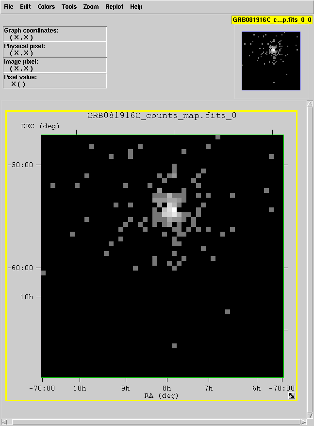 \")"
332 | ]
333 | },
334 | {
335 | "cell_type": "markdown",
336 | "metadata": {},
337 | "source": [
338 | "One readily observes that there are many pixels containing a few counts each near the burst location, and few pixels containing any counts away from the burst. It is also evident that the burst location is not centered in the counts map. This means the preliminary location sent out in the GCN was not quite the right location. This is not uncommon for automated transient localizations.\n",
339 | "\n",
340 | "Using *ds9* instead of *fv* allows us to find the location of the brightest pixel, and a better position for the burst."
341 | ]
342 | },
343 | {
344 | "cell_type": "code",
345 | "execution_count": null,
346 | "metadata": {},
347 | "outputs": [],
348 | "source": [
349 | "HTML(\"
\")"
332 | ]
333 | },
334 | {
335 | "cell_type": "markdown",
336 | "metadata": {},
337 | "source": [
338 | "One readily observes that there are many pixels containing a few counts each near the burst location, and few pixels containing any counts away from the burst. It is also evident that the burst location is not centered in the counts map. This means the preliminary location sent out in the GCN was not quite the right location. This is not uncommon for automated transient localizations.\n",
339 | "\n",
340 | "Using *ds9* instead of *fv* allows us to find the location of the brightest pixel, and a better position for the burst."
341 | ]
342 | },
343 | {
344 | "cell_type": "code",
345 | "execution_count": null,
346 | "metadata": {},
347 | "outputs": [],
348 | "source": [
349 | "HTML(\"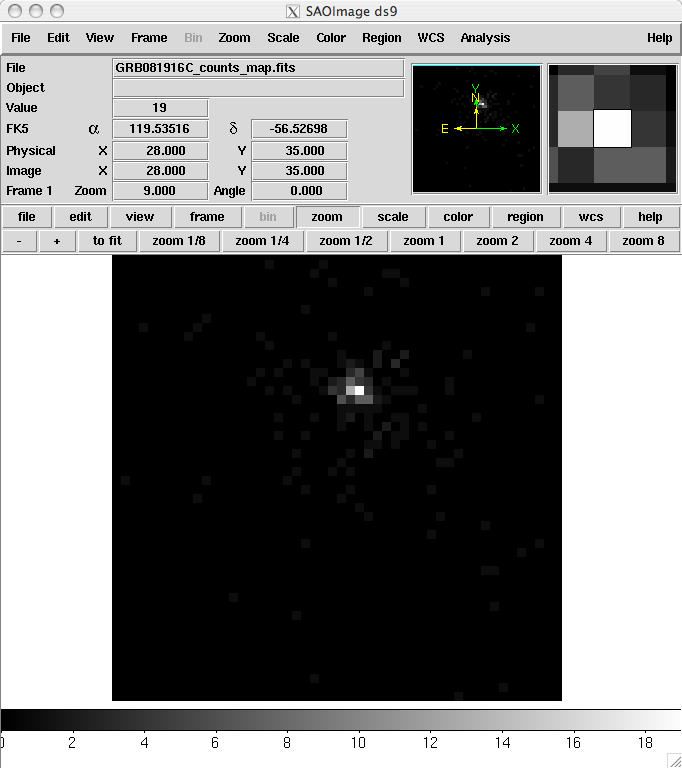 \")"
350 | ]
351 | },
352 | {
353 | "cell_type": "markdown",
354 | "metadata": {},
355 | "source": [
356 | "By simply mousing over that pixel, the RA and Dec of the likely burst location get displayed in the FK5 boxes (here, the new position is 119.5, -56.5). This is a quick method of localizing a burst, though not as accurate as fitting the data (described in the [Likelihood Tutorial](https://fermi.gsfc.nasa.gov/ssc/data/p6v11/analysis/scitools/likelihood_tutorial.html)).\n",
357 | "\n",
358 | "> **Note**: To change the *ds9* display for the mouseover from sexagesimal (the default) to degrees, go to the WCS menu and select \"Degrees\" in the bottom portion of the menu."
359 | ]
360 | },
361 | {
362 | "cell_type": "markdown",
363 | "metadata": {},
364 | "source": [
365 | "**To look at the lightcurve:**\n",
366 | "\n",
367 | "1. Open `GRB081916C_light_curve.fits` in *fv*.\n",
368 | "\n",
369 | " The lightcurve is in the RATE extension. Choose 'All' to view the content of that extension. The extension has 4 columns: TIME, TIMEDEL, COUNTS and ERROR.\n",
370 | " \n",
371 | " The time bins were created to have a width of 10 seconds, and therefore TIMEDEL is always 10.\n",
372 | " \n",
373 | "2. Now plot the COUNTS as a function of TIME. Select 'Plot' for the RATE extension. Click on 'Time' then on 'x'. Click on 'Counts' then on 'y'. Finally click on 'Plot'. The result is:"
374 | ]
375 | },
376 | {
377 | "cell_type": "code",
378 | "execution_count": null,
379 | "metadata": {},
380 | "outputs": [],
381 | "source": [
382 | "!fv ./data/GrB081916C_light_curve.fits"
383 | ]
384 | },
385 | {
386 | "cell_type": "code",
387 | "execution_count": null,
388 | "metadata": {},
389 | "outputs": [],
390 | "source": [
391 | "HTML(\"
\")"
350 | ]
351 | },
352 | {
353 | "cell_type": "markdown",
354 | "metadata": {},
355 | "source": [
356 | "By simply mousing over that pixel, the RA and Dec of the likely burst location get displayed in the FK5 boxes (here, the new position is 119.5, -56.5). This is a quick method of localizing a burst, though not as accurate as fitting the data (described in the [Likelihood Tutorial](https://fermi.gsfc.nasa.gov/ssc/data/p6v11/analysis/scitools/likelihood_tutorial.html)).\n",
357 | "\n",
358 | "> **Note**: To change the *ds9* display for the mouseover from sexagesimal (the default) to degrees, go to the WCS menu and select \"Degrees\" in the bottom portion of the menu."
359 | ]
360 | },
361 | {
362 | "cell_type": "markdown",
363 | "metadata": {},
364 | "source": [
365 | "**To look at the lightcurve:**\n",
366 | "\n",
367 | "1. Open `GRB081916C_light_curve.fits` in *fv*.\n",
368 | "\n",
369 | " The lightcurve is in the RATE extension. Choose 'All' to view the content of that extension. The extension has 4 columns: TIME, TIMEDEL, COUNTS and ERROR.\n",
370 | " \n",
371 | " The time bins were created to have a width of 10 seconds, and therefore TIMEDEL is always 10.\n",
372 | " \n",
373 | "2. Now plot the COUNTS as a function of TIME. Select 'Plot' for the RATE extension. Click on 'Time' then on 'x'. Click on 'Counts' then on 'y'. Finally click on 'Plot'. The result is:"
374 | ]
375 | },
376 | {
377 | "cell_type": "code",
378 | "execution_count": null,
379 | "metadata": {},
380 | "outputs": [],
381 | "source": [
382 | "!fv ./data/GrB081916C_light_curve.fits"
383 | ]
384 | },
385 | {
386 | "cell_type": "code",
387 | "execution_count": null,
388 | "metadata": {},
389 | "outputs": [],
390 | "source": [
391 | "HTML(\"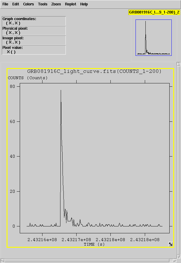 \")"
392 | ]
393 | },
394 | {
395 | "cell_type": "markdown",
396 | "metadata": {},
397 | "source": [
398 | ">**Note**: Except for the period of the burst, almost all bins have 0-5 counts. This demonstrates that there is very little background for LAT observations of gamma-ray bursts."
399 | ]
400 | }
401 | ],
402 | "metadata": {
403 | "kernelspec": {
404 | "display_name": "Python 3",
405 | "language": "python",
406 | "name": "python3"
407 | },
408 | "language_info": {
409 | "codemirror_mode": {
410 | "name": "ipython",
411 | "version": 3
412 | },
413 | "file_extension": ".py",
414 | "mimetype": "text/x-python",
415 | "name": "python",
416 | "nbconvert_exporter": "python",
417 | "pygments_lexer": "ipython3",
418 | "version": "3.7.9"
419 | }
420 | },
421 | "nbformat": 4,
422 | "nbformat_minor": 2
423 | }
424 |
--------------------------------------------------------------------------------
/DataSelection/5.UsingLATAllSkyWeekly/LAT_weekly_allsky.ipynb:
--------------------------------------------------------------------------------
1 | {
2 | "cells": [
3 | {
4 | "cell_type": "markdown",
5 | "metadata": {},
6 | "source": [
7 | "# Using Fermi-LAT All-sky Weekly Files\n",
8 | "\n",
9 | "Some types of data analyses lend themselves to the use of all-sky data files, rather than repeatedly downloading overlapping regions of sky for repeat analysis. Examples are:\n",
10 | "\n",
11 | "* Light curves and spectra for a large number of sources, whether galactic, extragalactic, or both\n",
12 | "* Characterization of large-scale diffuse emission\n",
13 | "* Analysis of moving sources, like the Sun\n",
14 | "* Searches for transient events (like GRBs) that have an isotropic distribution\n",
15 | "\n",
16 | "This analysis thread describes how to generate an all-sky data set for use in other types of analysis. We will then create an exposure-corrected all-sky image as an example of how to use the weekly files."
17 | ]
18 | },
19 | {
20 | "cell_type": "markdown",
21 | "metadata": {},
22 | "source": [
23 | "## Download the weekly LAT files\n",
24 | "\n",
25 | "The weekly LAT data files are available from the FSSC [FTP Server](https://heasarc.gsfc.nasa.gov/FTP/fermi/data/lat/). These files contain the LAT data acquired during each week of Fermi's science mission. (Mission weeks run Thursday through Wednesday, UTC time.) The file for the current mission week will also be listed, even though the week may not yet be complete.\n",
26 | "\n",
27 | "The current mission week file is regenerated by the FSSC after every data delivery from the LAT instrument team. This guarantees that the FTP Server and the LAT data server contain the same data, and both are up-to-date.\n",
28 | "\n",
29 | "You can download the LAT weekly files one at a time from the FTP site, or you can use `wget` to download a full set of files.\n",
30 | "\n",
31 | "Once you have the current set of files, you can use the same `wget` command (from the same directory) to download only the newest files. In the event that the LAT team reprocesses data for the full mission, the filenames will change, and `wget` will download a full set of the new, reprocessed, data.\n",
32 | "\n",
33 | ">**Note**: This may take a while."
34 | ]
35 | },
36 | {
37 | "cell_type": "code",
38 | "execution_count": null,
39 | "metadata": {},
40 | "outputs": [],
41 | "source": [
42 | "!wget -m -P . -nH --cut-dirs=4 -np -e robots=off https://heasarc.gsfc.nasa.gov/FTP/fermi/data/lat/weekly/photon/"
43 | ]
44 | },
45 | {
46 | "cell_type": "markdown",
47 | "metadata": {},
48 | "source": [
49 | "LAT data has been classified based on the quality of the event reconstruction. The classification can then be used to reduce background and improve performance by filtering out poorly reconstructed events.\n",
50 | "\n",
51 | "With the advent of Pass 8 data reconstruction, there are a myriad of various event classes that are tailored for specific types of analysis. The user should see the [Cicerone](https://fermi.gsfc.nasa.gov/ssc/data/analysis/documentation/Cicerone/Cicerone_Data_Exploration/Data_preparation.html) pages for a full description of the various event classes (and types) available in Pass 8.\n",
52 | "\n",
53 | "For most analyses, the user will be interested in `SOURCE` class photons (`evclass=128`). However, analyses that are intrinsically signal limited require very low background. For example, a user studying large scale, diffuse structures may be interested in using the `CLEAN` (`evclass=256`) or even `ULTRACLEAN` (`evclass=512`) classes.\n",
54 | "\n",
55 | "There are two types of weekly files available; photon files and extended files. The photon weekly files contain all the SOURCE class and are usable for most analyses. The extended files contain the same events as the photon files, but also contain additional reconstruction information about each photon that may be useful if you are trying to characterize the quality of a particular signal, such as for dark matter line searches.\n",
56 | "\n",
57 | ">**NOTE**: For analysis of short timescale events (for example, GRBs) where the flux of the event is much brighter than the accrued background, the user may be interested in using the `TRANSIENT010` (`evclass=64`) event class. If you are interested in investigating transient events within LAT data, you cannot use the weekly files, as they have been prefiltered to contain SOURCE class photons. There are no weekly files that contain the `TRANSIENT` class events.\n",
58 | ">\n",
59 | ">In order to generate an all-sky dataset of `TRANSIENT` class events, you will need to perform a grid of [data server](https://fermi.gsfc.nasa.gov/cgi-bin/ssc/LAT/LATDataQuery.cgi) queries with the maximum radius of 60 degrees. Once you have downloaded data from the full sky, you will need to combine the files and filter out duplicate events. We recommend using the [FTOOLS](https://heasarc.gsfc.nasa.gov/lheasoft/ftools/ftools_menu.html) suite to perform these tasks.\n",
60 | "\n",
61 | "Run this command to download the weekly extended files:"
62 | ]
63 | },
64 | {
65 | "cell_type": "code",
66 | "execution_count": null,
67 | "metadata": {},
68 | "outputs": [],
69 | "source": [
70 | "!wget -m -P . -nH --cut-dirs=4 -np -e robots=off https://heasarc.gsfc.nasa.gov/FTP/fermi/data/lat/weekly/extended/"
71 | ]
72 | },
73 | {
74 | "cell_type": "markdown",
75 | "metadata": {},
76 | "source": [
77 | "In order to do analysis for the full mission, you will also need the mission-long spacecraft file. This file contains entries at 30-second intervals during all periods of active data-taking by the LAT instrument. As a result, this file can be rather large.\n",
78 | "\n",
79 | "There are also weekly spacecraft files that contain the same information. However, some users have found the pre-generated full mission file to be more robust during analysis than a concatenated set of weekly files.\n",
80 | "\n",
81 | "We recommend re-downloading the full mission file when you update your all-sky data set.\n",
82 | "\n",
83 | "Run this command to download the mission spacecraft file:"
84 | ]
85 | },
86 | {
87 | "cell_type": "code",
88 | "execution_count": null,
89 | "metadata": {},
90 | "outputs": [],
91 | "source": [
92 | "!wget -m -P . -nH --cut-dirs=4 -np -e robots=off https://heasarc.gsfc.nasa.gov/FTP/fermi/data/lat/mission/spacecraft/"
93 | ]
94 | },
95 | {
96 | "cell_type": "markdown",
97 | "metadata": {},
98 | "source": [
99 | "# Combine the data files\n",
100 | "\n",
101 | "You should now have a full set of weekly files and a mission-long spacecraft file. The next step is to combine the weekly files into a single file. We will use the [gtselect](https://fermi.gsfc.nasa.gov/ssc/data/analysis/scitools/help/gtselect.txt) tool which can also be used for filtering data. But we want to combine the full data set without removing any events, so we will use slightly different parameters.\n",
102 | "\n",
103 | "To combine files, we first create a file list:"
104 | ]
105 | },
106 | {
107 | "cell_type": "code",
108 | "execution_count": null,
109 | "metadata": {},
110 | "outputs": [],
111 | "source": [
112 | "!mkdir ./data\n",
113 | "!ls ./weekly/photon/lat_photon_weekly* > ./data/filelist.txt"
114 | ]
115 | },
116 | {
117 | "cell_type": "code",
118 | "execution_count": null,
119 | "metadata": {},
120 | "outputs": [],
121 | "source": [
122 | "!cat ./data/filelist.txt"
123 | ]
124 | },
125 | {
126 | "cell_type": "markdown",
127 | "metadata": {},
128 | "source": [
129 | "If you look at filelist.txt, you will see it is simply a list of all the files in the directory that start with the string `lat_photon_weekly`. You will also want to clear any parameters in gtselect from previous analysis that could inadvertently remove events from the dataset.\n",
130 | "\n",
131 | "Clear the **gtselect** parameter file back to defaults with the command:"
132 | ]
133 | },
134 | {
135 | "cell_type": "code",
136 | "execution_count": null,
137 | "metadata": {},
138 | "outputs": [],
139 | "source": [
140 | "!punlearn gtselect"
141 | ]
142 | },
143 | {
144 | "cell_type": "markdown",
145 | "metadata": {},
146 | "source": [
147 | "Now you're ready to run [gtselect](https://fermi.gsfc.nasa.gov/ssc/data/analysis/scitools/help/gtselect.txt) to combine the data files. Here we will use `INDEF` so that gtselect will not make a selection on event class or event type. See the **gtselect** [help file](https://fermi.gsfc.nasa.gov/ssc/data/analysis/scitools/help/gtselect.txt) for a description of the evclass and evtype cuts."
148 | ]
149 | },
150 | {
151 | "cell_type": "code",
152 | "execution_count": null,
153 | "metadata": {},
154 | "outputs": [],
155 | "source": [
156 | "%%bash\n",
157 | "gtselect evclass=INDEF evtype=INDEF\n",
158 | " @./data/filelist.txt\n",
159 | " ./data/lat_alldata.fits\n",
160 | " 0\n",
161 | " 0\n",
162 | " 180\n",
163 | " INDEF\n",
164 | " INDEF\n",
165 | " 30\n",
166 | " 1000000\n",
167 | " 180"
168 | ]
169 | },
170 | {
171 | "cell_type": "markdown",
172 | "metadata": {},
173 | "source": [
174 | "Combining the files may take a while.\n",
175 | "\n",
176 | "Now that you have mission-long data and spacecraft files, you are ready to generate AGN light curves, search for flaring sources, or perform any other type of analysis that requires using data from many regions on the sky. A simple example is described below."
177 | ]
178 | },
179 | {
180 | "cell_type": "markdown",
181 | "metadata": {},
182 | "source": [
183 | "# Using the LAT data to produce an all-sky image"
184 | ]
185 | },
186 | {
187 | "cell_type": "markdown",
188 | "metadata": {},
189 | "source": [
190 | "### Step 1: Remove limb photons"
191 | ]
192 | },
193 | {
194 | "cell_type": "markdown",
195 | "metadata": {},
196 | "source": [
197 | "First, filter the data for the proper event class and to remove the earth limb contamination.\n",
198 | "\n",
199 | "We will use the `SOURCE` class (`evclass=128`) as it has been tuned to balance statistics with background for long-duration point source analysis.\n",
200 | "\n",
201 | "Here we also include the `evtype=3` cut to use both front and back converting event types. We will remove contamination by limiting the reconstructed zenith angle to events at an angle of 90° or less. We will also improve the PSF by excluding events with reconstructed energies below 1 GeV.\n",
202 | "\n",
203 | "Run [gtselect](https://fermi.gsfc.nasa.gov/ssc/data/analysis/scitools/help/gtselect.txt) to filter the data and apply a zenith cut."
204 | ]
205 | },
206 | {
207 | "cell_type": "code",
208 | "execution_count": null,
209 | "metadata": {},
210 | "outputs": [],
211 | "source": [
212 | "%%bash\n",
213 | "gtselect\n",
214 | " ./data/lat_alldata.fits\n",
215 | " ./data/lat_source_zmax90_gt1gev.fits\n",
216 | " 0\n",
217 | " 0\n",
218 | " 180\n",
219 | " INDEF\n",
220 | " INDEF\n",
221 | " 1000\n",
222 | " 500000\n",
223 | " 90"
224 | ]
225 | },
226 | {
227 | "cell_type": "markdown",
228 | "metadata": {},
229 | "source": [
230 | "Next, correct the exposure for the events you filtered out.\n",
231 | "\n",
232 | "The way the Fermitools account for exposure is computed based on the Good Time Intervals (GTIs) recorded in the event file. Because we have eliminated some events, we need to update the GTIs for the filtered file. Even though we have used a zenith cut on the data, we will not correct for it here.\n",
233 | "\n",
234 | "For an all-sky analysis, an ROI-based zenith cut would eliminate the entire dataset. Instead, we will later correct the livetime calculation for the zenith angle cut made with [gtselect](https://fermi.gsfc.nasa.gov/ssc/data/analysis/scitools/help/gtselect.txt).\n",
235 | "\n",
236 | "The [gtmktime tool](https://fermi.gsfc.nasa.gov/ssc/data/analysis/scitools/help/gtmktime.txt) updates the GTI list based on events we eliminated in the previous step. It also provides the ability to filter on any of the parameters stored in the spacecraft pointing history file. We will use the most basic filter recommended by the LAT team."
237 | ]
238 | },
239 | {
240 | "cell_type": "code",
241 | "execution_count": null,
242 | "metadata": {},
243 | "outputs": [],
244 | "source": [
245 | "%%bash\n",
246 | "gtmktime\n",
247 | " ./mission/spacecraft/lat_spacecraft_merged.fits\n",
248 | " (DATA_QUAL>0)&&(LAT_CONFIG==1)\n",
249 | " no\n",
250 | " ./data/lat_source_zmax90_gt1gev.fits\n",
251 | " ./data/lat_source_zmax90_gt1gev_gti.fits"
252 | ]
253 | },
254 | {
255 | "cell_type": "markdown",
256 | "metadata": {},
257 | "source": [
258 | "### Step 2: Bin the data\n",
259 | "\n",
260 | "Now you will bin the data in preparation for exposure correction. In order to correct the map for exposure, you have to account for the changing response with energy. To do this, bin the data into a counts cube using [gtbin](https://fermi.gsfc.nasa.gov/ssc/data/analysis/scitools/help/gtbin.txt), but with a single energy bin."
261 | ]
262 | },
263 | {
264 | "cell_type": "code",
265 | "execution_count": null,
266 | "metadata": {},
267 | "outputs": [],
268 | "source": [
269 | "%%bash\n",
270 | "gtbin\n",
271 | " CCUBE\n",
272 | " ./data/lat_source_zmax90_gt1gev_gti.fits\n",
273 | " ./data/lat_source_zmax90_gt1gev_ccube.fits\n",
274 | " ./mission/spacecraft/lat_spacecraft_merged.fits\n",
275 | " 3600\n",
276 | " 1800\n",
277 | " 0.1\n",
278 | " GAL\n",
279 | " 0\n",
280 | " 0\n",
281 | " 0\n",
282 | " AIT\n",
283 | " LOG\n",
284 | " 1000\n",
285 | " 500000\n",
286 | " 1"
287 | ]
288 | },
289 | {
290 | "cell_type": "markdown",
291 | "metadata": {},
292 | "source": [
293 | "### Step 3: Calculate exposure map\n",
294 | "\n",
295 | "Because Fermi data are sparse, the accumulated exposure time for any given point in the sky is based on the observatory's pointing history and the response of the instrument to events at various incidence angles and different energies.\n",
296 | "\n",
297 | "The LAT team has calculated how the instrument responds by modeling the entire instrument and then running a MonteCarlo simulation of many millions of events of different energies and directions. These simulations characterize how the gamma rays propagate through an ideal instrument, and the information is recorded in the Instrument Response Functions (IRF). Since the response depends on how much data filtering is performed, there are different IRFs for the different event classes.\n",
298 | "\n",
299 | "To see which IRFs are available from within the Fermitools, run the [gtirfs](https://fermi.gsfc.nasa.gov/ssc/data/analysis/scitools/help/gtirfs.txt) command."
300 | ]
301 | },
302 | {
303 | "cell_type": "code",
304 | "execution_count": null,
305 | "metadata": {},
306 | "outputs": [],
307 | "source": [
308 | "!gtirfs"
309 | ]
310 | },
311 | {
312 | "cell_type": "markdown",
313 | "metadata": {},
314 | "source": [
315 | "The appropriate IRF for this data set is `P8R3_SOURCE_V2`.\n",
316 | "\n",
317 | "Calculating exposure for an all-sky map first requires calculating the instrument livetime for the entire sky (using [gtltcube](https://fermi.gsfc.nasa.gov/ssc/data/analysis/scitools/help/gtltcube.txt)) and then convolving the livetime with the IRF (using [gtexpmap2](https://fermi.gsfc.nasa.gov/ssc/data/analysis/scitools/help/gtexpmap.txt)).\n",
318 | "\n",
319 | "The pixel size for the livetime does not need to match the binned data, but you do need to provide the event file as [gtltcube](https://fermi.gsfc.nasa.gov/ssc/data/analysis/scitools/help/gtltcube.txt) uses the good time intervals to calculate the livetime at each position.\n",
320 | "\n",
321 | "You will also need to correct the livetime for the zenith angle cut made with [gtselect](https://fermi.gsfc.nasa.gov/ssc/data/analysis/scitools/help/gtselect.txt) earlier. To do this, use the `zmax` option on the command line and match the value used with [gtselect](https://fermi.gsfc.nasa.gov/ssc/data/analysis/scitools/help/gtselect.txt). This modifies the livetime calculation to account for the events you removed earlier.\n",
322 | "Here is an example of the input for [gtltcube](https://fermi.gsfc.nasa.gov/ssc/data/analysis/scitools/help/gtltcube.txt):"
323 | ]
324 | },
325 | {
326 | "cell_type": "code",
327 | "execution_count": null,
328 | "metadata": {},
329 | "outputs": [],
330 | "source": [
331 | "%%bash\n",
332 | "gtltcube zmax=90\n",
333 | " ./data/lat_source_zmax90_gt1gev_gti.fits\n",
334 | " ./mission/spacecraft/lat_spacecraft_merged.fits\n",
335 | " ./data/lat_source_zmax90_gt1gev_ltcube.fits\n",
336 | " 0.025\n",
337 | " 1"
338 | ]
339 | },
340 | {
341 | "cell_type": "markdown",
342 | "metadata": {},
343 | "source": [
344 | "Now you can calculate the exposure at each point in the sky in each energy bin (we used only one bin) using [gtexpcube2](https://fermi.gsfc.nasa.gov/ssc/data/analysis/scitools/help/gtexpcube2.txt).\n",
345 | "\n",
346 | "You will need to enter the pixel geometry and energy binning to match what you used in the counts cube.\n",
347 | "\n",
348 | "Also, be sure to use `CENTER` for the energy layer reference. If you use `EDGE`, you will get an additional energy plane in the output file that causes complications later."
349 | ]
350 | },
351 | {
352 | "cell_type": "code",
353 | "execution_count": null,
354 | "metadata": {},
355 | "outputs": [],
356 | "source": [
357 | "%%bash\n",
358 | "gtexpcube2\n",
359 | " ./data/lat_source_zmax90_gt1gev_ltcube.fits\n",
360 | " none\n",
361 | " ./data/lat_source_zmax90_gt1gev_expcube1.fits\n",
362 | " P8R3_SOURCE_V3\n",
363 | " 3600\n",
364 | " 1800\n",
365 | " 0.1\n",
366 | " 0\n",
367 | " 0\n",
368 | " 0\n",
369 | " AIT\n",
370 | " GAL\n",
371 | " 1000\n",
372 | " 500000\n",
373 | " 1"
374 | ]
375 | },
376 | {
377 | "cell_type": "markdown",
378 | "metadata": {},
379 | "source": [
380 | "**Note**: You could use CALDB for the IRF, but if this doesn't work, try explicitly specifying the IRF. The appropriate IRF for this data set is `P8R3_SOURCE_V3`.\n",
381 | "\n",
382 | "If you open the exposure map with _ds9_, you will see that the image has two energy planes. The first plane is for 1-300 GeV, the second is for 300 GeV and above. We will only use the first image plane to correct our all-sky map."
383 | ]
384 | },
385 | {
386 | "cell_type": "markdown",
387 | "metadata": {},
388 | "source": [
389 | "### Step 4: Correct the all-sky image for exposure and scale\n",
390 | "\n",
391 | "To complete the exposure correction, you must perform a set of arithmetic functions on the all-sky counts cube using the [FTOOLS](https://heasarc.nasa.gov/lheasoft/ftools/ftools_subpacks.html) **fextract**, **faith**, **fimgtrim**, and **fcarith**. First, extract the first of the two exposure planes:"
392 | ]
393 | },
394 | {
395 | "cell_type": "code",
396 | "execution_count": null,
397 | "metadata": {},
398 | "outputs": [],
399 | "source": [
400 | "%%bash\n",
401 | "fextract\n",
402 | " ./data/lat_source_zmax90_gt1gev_expcube1.fits[0]\n",
403 | " ./data/testfextract.fits"
404 | ]
405 | },
406 | {
407 | "cell_type": "markdown",
408 | "metadata": {},
409 | "source": [
410 | "Next, correct the value of each pixel for the exposure:"
411 | ]
412 | },
413 | {
414 | "cell_type": "code",
415 | "execution_count": null,
416 | "metadata": {},
417 | "outputs": [],
418 | "source": [
419 | "%%bash\n",
420 | "farith\n",
421 | " ./data/lat_source_zmax90_gt1gev_ccube.fits\n",
422 | " ./data/lat_source_zmax90_gt1gev_expcube1.fits\n",
423 | " ./data/lat_source_zmax90_gt1gev_corrmap.fits\n",
424 | " DIV"
425 | ]
426 | },
427 | {
428 | "cell_type": "markdown",
429 | "metadata": {},
430 | "source": [
431 | "Then trim the pixels that were outside the Aitoff projection to zero so they don't affect your display."
432 | ]
433 | },
434 | {
435 | "cell_type": "code",
436 | "execution_count": null,
437 | "metadata": {},
438 | "outputs": [],
439 | "source": [
440 | "%%bash\n",
441 | "fimgtrim\n",
442 | " ./data/lat_source_zmax90_gt1gev_corrmap.fits\n",
443 | " 0\n",
444 | " 0\n",
445 | " INDEF\n",
446 | " ./data/lat_source_zmax90_gt1gev_corrmap2.fits"
447 | ]
448 | },
449 | {
450 | "cell_type": "markdown",
451 | "metadata": {},
452 | "source": [
453 | "Finally, scale the image so that the maximum pixel is equal to 255 (the typical maximum dynamic range for graphics).\n",
454 | "\n",
455 | "There are a number of ways to find the maximum pixel value. Here we have used _ds9_ to find a maximum pixel value of $4.143x10^{-8}$. This means our scale factor should be $255/4.143x10^{-8}$, or $6.155x10^9$."
456 | ]
457 | },
458 | {
459 | "cell_type": "code",
460 | "execution_count": null,
461 | "metadata": {},
462 | "outputs": [],
463 | "source": [
464 | "%%bash\n",
465 | "fcarith\n",
466 | " ./data/lat_source_zmax90_gt1gev_corrmap2.fits\n",
467 | " 6.155e9\n",
468 | " ./data/lat_source_zmax90_gt1gev_corrmap3.fits\n",
469 | " MUL"
470 | ]
471 | },
472 | {
473 | "cell_type": "markdown",
474 | "metadata": {},
475 | "source": [
476 | "You can look at the final product in _ds9_ using log scaling. This process is approximately the same as is used to create the LAT all-sky images released by the instrument team.\n",
477 | "\n",
478 | "This method can be used for different energy ranges, different event class selections, or even to compare different data sets."
479 | ]
480 | }
481 | ],
482 | "metadata": {
483 | "kernelspec": {
484 | "display_name": "Python 3",
485 | "language": "python",
486 | "name": "python3"
487 | },
488 | "language_info": {
489 | "codemirror_mode": {
490 | "name": "ipython",
491 | "version": 3
492 | },
493 | "file_extension": ".py",
494 | "mimetype": "text/x-python",
495 | "name": "python",
496 | "nbconvert_exporter": "python",
497 | "pygments_lexer": "ipython3",
498 | "version": "3.7.9"
499 | }
500 | },
501 | "nbformat": 4,
502 | "nbformat_minor": 2
503 | }
504 |
--------------------------------------------------------------------------------
/LICENSE:
--------------------------------------------------------------------------------
1 | MIT License
2 |
3 | Copyright (c) 2019 Fermi Gamma-Ray Space Telescope
4 |
5 | Permission is hereby granted, free of charge, to any person obtaining a copy
6 | of this software and associated documentation files (the "Software"), to deal
7 | in the Software without restriction, including without limitation the rights
8 | to use, copy, modify, merge, publish, distribute, sublicense, and/or sell
9 | copies of the Software, and to permit persons to whom the Software is
10 | furnished to do so, subject to the following conditions:
11 |
12 | The above copyright notice and this permission notice shall be included in all
13 | copies or substantial portions of the Software.
14 |
15 | THE SOFTWARE IS PROVIDED "AS IS", WITHOUT WARRANTY OF ANY KIND, EXPRESS OR
16 | IMPLIED, INCLUDING BUT NOT LIMITED TO THE WARRANTIES OF MERCHANTABILITY,
17 | FITNESS FOR A PARTICULAR PURPOSE AND NONINFRINGEMENT. IN NO EVENT SHALL THE
18 | AUTHORS OR COPYRIGHT HOLDERS BE LIABLE FOR ANY CLAIM, DAMAGES OR OTHER
19 | LIABILITY, WHETHER IN AN ACTION OF CONTRACT, TORT OR OTHERWISE, ARISING FROM,
20 | OUT OF OR IN CONNECTION WITH THE SOFTWARE OR THE USE OR OTHER DEALINGS IN THE
21 | SOFTWARE.
22 |
--------------------------------------------------------------------------------
/ObsSim/1.ObservationSim/obssim_tutorial.ipynb:
--------------------------------------------------------------------------------
1 | {
2 | "cells": [
3 | {
4 | "cell_type": "markdown",
5 | "metadata": {},
6 | "source": [
7 | "# Observation Simulation Tutorial\n",
8 | "\n",
9 | "This tutorial provides some step-by-step examples of how to simulate Fermi observations using the [gtobssim](https://fermi.gsfc.nasa.gov/ssc/data/analysis/scitools/help/gtobssim.txt) application.\n",
10 | "\n",
11 | "For example: a Guest Investigator planning a proposal may need to make a realistic assessment of the detection significance achievable within a given time interval or the ability to constrain source model parameters for a given source intensity. More subtle issues may also be explored: e.g. how sensitive a given observation may be to pulsed emission of a given flux and modulation depth, spatially extended emission, or pointed versus survey mode observation scenarios.\n",
12 | "\n",
13 | "The [gtobssim](https://fermi.gsfc.nasa.gov/ssc/data/analysis/scitools/help/gtobssim.txt) tool (and related [gtorbsim](https://fermi.gsfc.nasa.gov/ssc/data/analysis/scitools/help/gtorbsim.txt) tool) produce Fermi simulated data files. Which can then be analyzed with the Fermitools following the same procedure as with the real data.\n",
14 | "\n",
15 | "This tutorial assumes the user has a spacecraft data file already generated with the [gtorbsim](https://fermi.gsfc.nasa.gov/ssc/data/analysis/scitools/help/gtorbsim.txt) tool, or that he or she has obtained a sample spacecraft data file from the [FSSC website](https://fermi.gsfc.nasa.gov/ssc/) (step 4). Alternatively, for basic zenith-rocking scenarios, one can be created \"on the fly\"."
16 | ]
17 | },
18 | {
19 | "cell_type": "markdown",
20 | "metadata": {},
21 | "source": [
22 | "**Steps**:\n",
23 | "\n",
24 | "1. **Download the latest model for the isotropic background.**\n",
25 | "\n",
26 | " To simulate the background, you will need to download the necessary files that specify the Galactic interstellar emission and the isotropic component. For Pass 8 this is more complicated than with previous data releases because of the number of data selection options. In all cases the Galactic file is `gll_iem_v06.fits`. For standard analysis using SOURCE class (FRONT+BACK), the isotropic spectral template is `iso_P8R3_SOURCE_V2.txt`.\n",
27 | "\n",
28 | "\n",
29 | "2. **Prepare XML source library files**\n",
30 | "\n",
31 | " These are XML files containing the source model definitions used by [gtobssim](https://fermi.gsfc.nasa.gov/ssc/data/analysis/scitools/help/gtobssim.txt).\n",
32 | "\n",
33 | "\n",
34 | "3. **Create a list of XML input file names**\n",
35 | "\n",
36 | " Various XML source libraries already exist. In addition to creating custom libraries, you can make sources in these libraries available by including the full paths to the files in this list.\n",
37 | "\n",
38 | "\n",
39 | "4. **Create a list of sources**\n",
40 | "\n",
41 | " These are the sources to be modeled.\n",
42 | "\n",
43 | "\n",
44 | "5. **Specify or create a pointing and livetime history file**\n",
45 | "\n",
46 | " You can: use an existing pointing and livetime history file; create one using the [gtorbsim](https://fermi.gsfc.nasa.gov/ssc/data/analysis/scitools/help/gtorbsim.txt) tool; or define a pointing strategy and let [gtobssim](https://fermi.gsfc.nasa.gov/ssc/data/analysis/scitools/help/gtobssim.txt) compute one.\n",
47 | " \n",
48 | " \n",
49 | "6. **Run [gtobssim](https://fermi.gsfc.nasa.gov/ssc/data/analysis/scitools/help/gtobssim.txt)**"
50 | ]
51 | },
52 | {
53 | "cell_type": "markdown",
54 | "metadata": {},
55 | "source": [
56 | "# 1. Download the latest model for the isotropic background\n",
57 | "\n",
58 | "When you use the latest Galactic emission model `gll_iem_v06.fits` in a likelihood analysis, you will want to use a template for the isotropic diffuse emission, which includes the residual cosmic-ray background. For standard analysis you will need to download `iso_P8R3_SOURCE_V2.txt`. This is valid only for the `P8R3_SOURCE_V2` response function and only for data sets with front + back events combined.\n",
59 | "\n",
60 | "For isotropic spectral templates for other data selections, please see the Background Models page. The file `isotropic_allsky.fits` is also required. This is simply an image with all pixels set to a value of `1`."
61 | ]
62 | },
63 | {
64 | "cell_type": "markdown",
65 | "metadata": {},
66 | "source": [
67 | "# 2. Prepare the XML source library files\n",
68 | "\n",
69 | "These files contain the XML definitions of the sources that are used by [gtobssim](https://fermi.gsfc.nasa.gov/ssc/data/analysis/scitools/help/gtobssim.txt). These files by themselves are not valid XML documents, but rather they contain XML \"source_library\" tags that are compiled in memory into a valid XML document that is then parsed by the software. It should be noted that these files are analogous to, but unfortunately not compatible with gtlike xml source model files.\n",
70 | "\n",
71 | "The following example shows how to define point sources with simple and broken power-law spectra, diffuse sources using FITS image files as a templates in two different ways, and an isotropic diffuse source.\n",
72 | "\n",
73 | "The following xml files can be extracted from this document and edited with a text editor, or created with the model editor tool. Model editor creates models for **gtobssim** that are also available for **gtlike**. To use model editor tool, type:"
74 | ]
75 | },
76 | {
77 | "cell_type": "code",
78 | "execution_count": null,
79 | "metadata": {},
80 | "outputs": [],
81 | "source": [
82 | "!ModelEditor"
83 | ]
84 | },
85 | {
86 | "cell_type": "markdown",
87 | "metadata": {},
88 | "source": [
89 | "in the command line. The tool has its own help."
90 | ]
91 | },
92 | {
93 | "cell_type": "markdown",
94 | "metadata": {},
95 | "source": [
96 | "In this example, we specified source parameters derived from the Third EGRET Catalog, and incorporating the current Fermi background models."
97 | ]
98 | },
99 | {
100 | "cell_type": "code",
101 | "execution_count": 2,
102 | "metadata": {},
103 | "outputs": [],
104 | "source": [
105 | "!mkdir data"
106 | ]
107 | },
108 | {
109 | "cell_type": "code",
110 | "execution_count": 4,
111 | "metadata": {},
112 | "outputs": [],
113 | "source": [
114 | "with open('./data/example_library.xml', 'w') as file:\n",
115 | " file.write('''
\")"
392 | ]
393 | },
394 | {
395 | "cell_type": "markdown",
396 | "metadata": {},
397 | "source": [
398 | ">**Note**: Except for the period of the burst, almost all bins have 0-5 counts. This demonstrates that there is very little background for LAT observations of gamma-ray bursts."
399 | ]
400 | }
401 | ],
402 | "metadata": {
403 | "kernelspec": {
404 | "display_name": "Python 3",
405 | "language": "python",
406 | "name": "python3"
407 | },
408 | "language_info": {
409 | "codemirror_mode": {
410 | "name": "ipython",
411 | "version": 3
412 | },
413 | "file_extension": ".py",
414 | "mimetype": "text/x-python",
415 | "name": "python",
416 | "nbconvert_exporter": "python",
417 | "pygments_lexer": "ipython3",
418 | "version": "3.7.9"
419 | }
420 | },
421 | "nbformat": 4,
422 | "nbformat_minor": 2
423 | }
424 |
--------------------------------------------------------------------------------
/DataSelection/5.UsingLATAllSkyWeekly/LAT_weekly_allsky.ipynb:
--------------------------------------------------------------------------------
1 | {
2 | "cells": [
3 | {
4 | "cell_type": "markdown",
5 | "metadata": {},
6 | "source": [
7 | "# Using Fermi-LAT All-sky Weekly Files\n",
8 | "\n",
9 | "Some types of data analyses lend themselves to the use of all-sky data files, rather than repeatedly downloading overlapping regions of sky for repeat analysis. Examples are:\n",
10 | "\n",
11 | "* Light curves and spectra for a large number of sources, whether galactic, extragalactic, or both\n",
12 | "* Characterization of large-scale diffuse emission\n",
13 | "* Analysis of moving sources, like the Sun\n",
14 | "* Searches for transient events (like GRBs) that have an isotropic distribution\n",
15 | "\n",
16 | "This analysis thread describes how to generate an all-sky data set for use in other types of analysis. We will then create an exposure-corrected all-sky image as an example of how to use the weekly files."
17 | ]
18 | },
19 | {
20 | "cell_type": "markdown",
21 | "metadata": {},
22 | "source": [
23 | "## Download the weekly LAT files\n",
24 | "\n",
25 | "The weekly LAT data files are available from the FSSC [FTP Server](https://heasarc.gsfc.nasa.gov/FTP/fermi/data/lat/). These files contain the LAT data acquired during each week of Fermi's science mission. (Mission weeks run Thursday through Wednesday, UTC time.) The file for the current mission week will also be listed, even though the week may not yet be complete.\n",
26 | "\n",
27 | "The current mission week file is regenerated by the FSSC after every data delivery from the LAT instrument team. This guarantees that the FTP Server and the LAT data server contain the same data, and both are up-to-date.\n",
28 | "\n",
29 | "You can download the LAT weekly files one at a time from the FTP site, or you can use `wget` to download a full set of files.\n",
30 | "\n",
31 | "Once you have the current set of files, you can use the same `wget` command (from the same directory) to download only the newest files. In the event that the LAT team reprocesses data for the full mission, the filenames will change, and `wget` will download a full set of the new, reprocessed, data.\n",
32 | "\n",
33 | ">**Note**: This may take a while."
34 | ]
35 | },
36 | {
37 | "cell_type": "code",
38 | "execution_count": null,
39 | "metadata": {},
40 | "outputs": [],
41 | "source": [
42 | "!wget -m -P . -nH --cut-dirs=4 -np -e robots=off https://heasarc.gsfc.nasa.gov/FTP/fermi/data/lat/weekly/photon/"
43 | ]
44 | },
45 | {
46 | "cell_type": "markdown",
47 | "metadata": {},
48 | "source": [
49 | "LAT data has been classified based on the quality of the event reconstruction. The classification can then be used to reduce background and improve performance by filtering out poorly reconstructed events.\n",
50 | "\n",
51 | "With the advent of Pass 8 data reconstruction, there are a myriad of various event classes that are tailored for specific types of analysis. The user should see the [Cicerone](https://fermi.gsfc.nasa.gov/ssc/data/analysis/documentation/Cicerone/Cicerone_Data_Exploration/Data_preparation.html) pages for a full description of the various event classes (and types) available in Pass 8.\n",
52 | "\n",
53 | "For most analyses, the user will be interested in `SOURCE` class photons (`evclass=128`). However, analyses that are intrinsically signal limited require very low background. For example, a user studying large scale, diffuse structures may be interested in using the `CLEAN` (`evclass=256`) or even `ULTRACLEAN` (`evclass=512`) classes.\n",
54 | "\n",
55 | "There are two types of weekly files available; photon files and extended files. The photon weekly files contain all the SOURCE class and are usable for most analyses. The extended files contain the same events as the photon files, but also contain additional reconstruction information about each photon that may be useful if you are trying to characterize the quality of a particular signal, such as for dark matter line searches.\n",
56 | "\n",
57 | ">**NOTE**: For analysis of short timescale events (for example, GRBs) where the flux of the event is much brighter than the accrued background, the user may be interested in using the `TRANSIENT010` (`evclass=64`) event class. If you are interested in investigating transient events within LAT data, you cannot use the weekly files, as they have been prefiltered to contain SOURCE class photons. There are no weekly files that contain the `TRANSIENT` class events.\n",
58 | ">\n",
59 | ">In order to generate an all-sky dataset of `TRANSIENT` class events, you will need to perform a grid of [data server](https://fermi.gsfc.nasa.gov/cgi-bin/ssc/LAT/LATDataQuery.cgi) queries with the maximum radius of 60 degrees. Once you have downloaded data from the full sky, you will need to combine the files and filter out duplicate events. We recommend using the [FTOOLS](https://heasarc.gsfc.nasa.gov/lheasoft/ftools/ftools_menu.html) suite to perform these tasks.\n",
60 | "\n",
61 | "Run this command to download the weekly extended files:"
62 | ]
63 | },
64 | {
65 | "cell_type": "code",
66 | "execution_count": null,
67 | "metadata": {},
68 | "outputs": [],
69 | "source": [
70 | "!wget -m -P . -nH --cut-dirs=4 -np -e robots=off https://heasarc.gsfc.nasa.gov/FTP/fermi/data/lat/weekly/extended/"
71 | ]
72 | },
73 | {
74 | "cell_type": "markdown",
75 | "metadata": {},
76 | "source": [
77 | "In order to do analysis for the full mission, you will also need the mission-long spacecraft file. This file contains entries at 30-second intervals during all periods of active data-taking by the LAT instrument. As a result, this file can be rather large.\n",
78 | "\n",
79 | "There are also weekly spacecraft files that contain the same information. However, some users have found the pre-generated full mission file to be more robust during analysis than a concatenated set of weekly files.\n",
80 | "\n",
81 | "We recommend re-downloading the full mission file when you update your all-sky data set.\n",
82 | "\n",
83 | "Run this command to download the mission spacecraft file:"
84 | ]
85 | },
86 | {
87 | "cell_type": "code",
88 | "execution_count": null,
89 | "metadata": {},
90 | "outputs": [],
91 | "source": [
92 | "!wget -m -P . -nH --cut-dirs=4 -np -e robots=off https://heasarc.gsfc.nasa.gov/FTP/fermi/data/lat/mission/spacecraft/"
93 | ]
94 | },
95 | {
96 | "cell_type": "markdown",
97 | "metadata": {},
98 | "source": [
99 | "# Combine the data files\n",
100 | "\n",
101 | "You should now have a full set of weekly files and a mission-long spacecraft file. The next step is to combine the weekly files into a single file. We will use the [gtselect](https://fermi.gsfc.nasa.gov/ssc/data/analysis/scitools/help/gtselect.txt) tool which can also be used for filtering data. But we want to combine the full data set without removing any events, so we will use slightly different parameters.\n",
102 | "\n",
103 | "To combine files, we first create a file list:"
104 | ]
105 | },
106 | {
107 | "cell_type": "code",
108 | "execution_count": null,
109 | "metadata": {},
110 | "outputs": [],
111 | "source": [
112 | "!mkdir ./data\n",
113 | "!ls ./weekly/photon/lat_photon_weekly* > ./data/filelist.txt"
114 | ]
115 | },
116 | {
117 | "cell_type": "code",
118 | "execution_count": null,
119 | "metadata": {},
120 | "outputs": [],
121 | "source": [
122 | "!cat ./data/filelist.txt"
123 | ]
124 | },
125 | {
126 | "cell_type": "markdown",
127 | "metadata": {},
128 | "source": [
129 | "If you look at filelist.txt, you will see it is simply a list of all the files in the directory that start with the string `lat_photon_weekly`. You will also want to clear any parameters in gtselect from previous analysis that could inadvertently remove events from the dataset.\n",
130 | "\n",
131 | "Clear the **gtselect** parameter file back to defaults with the command:"
132 | ]
133 | },
134 | {
135 | "cell_type": "code",
136 | "execution_count": null,
137 | "metadata": {},
138 | "outputs": [],
139 | "source": [
140 | "!punlearn gtselect"
141 | ]
142 | },
143 | {
144 | "cell_type": "markdown",
145 | "metadata": {},
146 | "source": [
147 | "Now you're ready to run [gtselect](https://fermi.gsfc.nasa.gov/ssc/data/analysis/scitools/help/gtselect.txt) to combine the data files. Here we will use `INDEF` so that gtselect will not make a selection on event class or event type. See the **gtselect** [help file](https://fermi.gsfc.nasa.gov/ssc/data/analysis/scitools/help/gtselect.txt) for a description of the evclass and evtype cuts."
148 | ]
149 | },
150 | {
151 | "cell_type": "code",
152 | "execution_count": null,
153 | "metadata": {},
154 | "outputs": [],
155 | "source": [
156 | "%%bash\n",
157 | "gtselect evclass=INDEF evtype=INDEF\n",
158 | " @./data/filelist.txt\n",
159 | " ./data/lat_alldata.fits\n",
160 | " 0\n",
161 | " 0\n",
162 | " 180\n",
163 | " INDEF\n",
164 | " INDEF\n",
165 | " 30\n",
166 | " 1000000\n",
167 | " 180"
168 | ]
169 | },
170 | {
171 | "cell_type": "markdown",
172 | "metadata": {},
173 | "source": [
174 | "Combining the files may take a while.\n",
175 | "\n",
176 | "Now that you have mission-long data and spacecraft files, you are ready to generate AGN light curves, search for flaring sources, or perform any other type of analysis that requires using data from many regions on the sky. A simple example is described below."
177 | ]
178 | },
179 | {
180 | "cell_type": "markdown",
181 | "metadata": {},
182 | "source": [
183 | "# Using the LAT data to produce an all-sky image"
184 | ]
185 | },
186 | {
187 | "cell_type": "markdown",
188 | "metadata": {},
189 | "source": [
190 | "### Step 1: Remove limb photons"
191 | ]
192 | },
193 | {
194 | "cell_type": "markdown",
195 | "metadata": {},
196 | "source": [
197 | "First, filter the data for the proper event class and to remove the earth limb contamination.\n",
198 | "\n",
199 | "We will use the `SOURCE` class (`evclass=128`) as it has been tuned to balance statistics with background for long-duration point source analysis.\n",
200 | "\n",
201 | "Here we also include the `evtype=3` cut to use both front and back converting event types. We will remove contamination by limiting the reconstructed zenith angle to events at an angle of 90° or less. We will also improve the PSF by excluding events with reconstructed energies below 1 GeV.\n",
202 | "\n",
203 | "Run [gtselect](https://fermi.gsfc.nasa.gov/ssc/data/analysis/scitools/help/gtselect.txt) to filter the data and apply a zenith cut."
204 | ]
205 | },
206 | {
207 | "cell_type": "code",
208 | "execution_count": null,
209 | "metadata": {},
210 | "outputs": [],
211 | "source": [
212 | "%%bash\n",
213 | "gtselect\n",
214 | " ./data/lat_alldata.fits\n",
215 | " ./data/lat_source_zmax90_gt1gev.fits\n",
216 | " 0\n",
217 | " 0\n",
218 | " 180\n",
219 | " INDEF\n",
220 | " INDEF\n",
221 | " 1000\n",
222 | " 500000\n",
223 | " 90"
224 | ]
225 | },
226 | {
227 | "cell_type": "markdown",
228 | "metadata": {},
229 | "source": [
230 | "Next, correct the exposure for the events you filtered out.\n",
231 | "\n",
232 | "The way the Fermitools account for exposure is computed based on the Good Time Intervals (GTIs) recorded in the event file. Because we have eliminated some events, we need to update the GTIs for the filtered file. Even though we have used a zenith cut on the data, we will not correct for it here.\n",
233 | "\n",
234 | "For an all-sky analysis, an ROI-based zenith cut would eliminate the entire dataset. Instead, we will later correct the livetime calculation for the zenith angle cut made with [gtselect](https://fermi.gsfc.nasa.gov/ssc/data/analysis/scitools/help/gtselect.txt).\n",
235 | "\n",
236 | "The [gtmktime tool](https://fermi.gsfc.nasa.gov/ssc/data/analysis/scitools/help/gtmktime.txt) updates the GTI list based on events we eliminated in the previous step. It also provides the ability to filter on any of the parameters stored in the spacecraft pointing history file. We will use the most basic filter recommended by the LAT team."
237 | ]
238 | },
239 | {
240 | "cell_type": "code",
241 | "execution_count": null,
242 | "metadata": {},
243 | "outputs": [],
244 | "source": [
245 | "%%bash\n",
246 | "gtmktime\n",
247 | " ./mission/spacecraft/lat_spacecraft_merged.fits\n",
248 | " (DATA_QUAL>0)&&(LAT_CONFIG==1)\n",
249 | " no\n",
250 | " ./data/lat_source_zmax90_gt1gev.fits\n",
251 | " ./data/lat_source_zmax90_gt1gev_gti.fits"
252 | ]
253 | },
254 | {
255 | "cell_type": "markdown",
256 | "metadata": {},
257 | "source": [
258 | "### Step 2: Bin the data\n",
259 | "\n",
260 | "Now you will bin the data in preparation for exposure correction. In order to correct the map for exposure, you have to account for the changing response with energy. To do this, bin the data into a counts cube using [gtbin](https://fermi.gsfc.nasa.gov/ssc/data/analysis/scitools/help/gtbin.txt), but with a single energy bin."
261 | ]
262 | },
263 | {
264 | "cell_type": "code",
265 | "execution_count": null,
266 | "metadata": {},
267 | "outputs": [],
268 | "source": [
269 | "%%bash\n",
270 | "gtbin\n",
271 | " CCUBE\n",
272 | " ./data/lat_source_zmax90_gt1gev_gti.fits\n",
273 | " ./data/lat_source_zmax90_gt1gev_ccube.fits\n",
274 | " ./mission/spacecraft/lat_spacecraft_merged.fits\n",
275 | " 3600\n",
276 | " 1800\n",
277 | " 0.1\n",
278 | " GAL\n",
279 | " 0\n",
280 | " 0\n",
281 | " 0\n",
282 | " AIT\n",
283 | " LOG\n",
284 | " 1000\n",
285 | " 500000\n",
286 | " 1"
287 | ]
288 | },
289 | {
290 | "cell_type": "markdown",
291 | "metadata": {},
292 | "source": [
293 | "### Step 3: Calculate exposure map\n",
294 | "\n",
295 | "Because Fermi data are sparse, the accumulated exposure time for any given point in the sky is based on the observatory's pointing history and the response of the instrument to events at various incidence angles and different energies.\n",
296 | "\n",
297 | "The LAT team has calculated how the instrument responds by modeling the entire instrument and then running a MonteCarlo simulation of many millions of events of different energies and directions. These simulations characterize how the gamma rays propagate through an ideal instrument, and the information is recorded in the Instrument Response Functions (IRF). Since the response depends on how much data filtering is performed, there are different IRFs for the different event classes.\n",
298 | "\n",
299 | "To see which IRFs are available from within the Fermitools, run the [gtirfs](https://fermi.gsfc.nasa.gov/ssc/data/analysis/scitools/help/gtirfs.txt) command."
300 | ]
301 | },
302 | {
303 | "cell_type": "code",
304 | "execution_count": null,
305 | "metadata": {},
306 | "outputs": [],
307 | "source": [
308 | "!gtirfs"
309 | ]
310 | },
311 | {
312 | "cell_type": "markdown",
313 | "metadata": {},
314 | "source": [
315 | "The appropriate IRF for this data set is `P8R3_SOURCE_V2`.\n",
316 | "\n",
317 | "Calculating exposure for an all-sky map first requires calculating the instrument livetime for the entire sky (using [gtltcube](https://fermi.gsfc.nasa.gov/ssc/data/analysis/scitools/help/gtltcube.txt)) and then convolving the livetime with the IRF (using [gtexpmap2](https://fermi.gsfc.nasa.gov/ssc/data/analysis/scitools/help/gtexpmap.txt)).\n",
318 | "\n",
319 | "The pixel size for the livetime does not need to match the binned data, but you do need to provide the event file as [gtltcube](https://fermi.gsfc.nasa.gov/ssc/data/analysis/scitools/help/gtltcube.txt) uses the good time intervals to calculate the livetime at each position.\n",
320 | "\n",
321 | "You will also need to correct the livetime for the zenith angle cut made with [gtselect](https://fermi.gsfc.nasa.gov/ssc/data/analysis/scitools/help/gtselect.txt) earlier. To do this, use the `zmax` option on the command line and match the value used with [gtselect](https://fermi.gsfc.nasa.gov/ssc/data/analysis/scitools/help/gtselect.txt). This modifies the livetime calculation to account for the events you removed earlier.\n",
322 | "Here is an example of the input for [gtltcube](https://fermi.gsfc.nasa.gov/ssc/data/analysis/scitools/help/gtltcube.txt):"
323 | ]
324 | },
325 | {
326 | "cell_type": "code",
327 | "execution_count": null,
328 | "metadata": {},
329 | "outputs": [],
330 | "source": [
331 | "%%bash\n",
332 | "gtltcube zmax=90\n",
333 | " ./data/lat_source_zmax90_gt1gev_gti.fits\n",
334 | " ./mission/spacecraft/lat_spacecraft_merged.fits\n",
335 | " ./data/lat_source_zmax90_gt1gev_ltcube.fits\n",
336 | " 0.025\n",
337 | " 1"
338 | ]
339 | },
340 | {
341 | "cell_type": "markdown",
342 | "metadata": {},
343 | "source": [
344 | "Now you can calculate the exposure at each point in the sky in each energy bin (we used only one bin) using [gtexpcube2](https://fermi.gsfc.nasa.gov/ssc/data/analysis/scitools/help/gtexpcube2.txt).\n",
345 | "\n",
346 | "You will need to enter the pixel geometry and energy binning to match what you used in the counts cube.\n",
347 | "\n",
348 | "Also, be sure to use `CENTER` for the energy layer reference. If you use `EDGE`, you will get an additional energy plane in the output file that causes complications later."
349 | ]
350 | },
351 | {
352 | "cell_type": "code",
353 | "execution_count": null,
354 | "metadata": {},
355 | "outputs": [],
356 | "source": [
357 | "%%bash\n",
358 | "gtexpcube2\n",
359 | " ./data/lat_source_zmax90_gt1gev_ltcube.fits\n",
360 | " none\n",
361 | " ./data/lat_source_zmax90_gt1gev_expcube1.fits\n",
362 | " P8R3_SOURCE_V3\n",
363 | " 3600\n",
364 | " 1800\n",
365 | " 0.1\n",
366 | " 0\n",
367 | " 0\n",
368 | " 0\n",
369 | " AIT\n",
370 | " GAL\n",
371 | " 1000\n",
372 | " 500000\n",
373 | " 1"
374 | ]
375 | },
376 | {
377 | "cell_type": "markdown",
378 | "metadata": {},
379 | "source": [
380 | "**Note**: You could use CALDB for the IRF, but if this doesn't work, try explicitly specifying the IRF. The appropriate IRF for this data set is `P8R3_SOURCE_V3`.\n",
381 | "\n",
382 | "If you open the exposure map with _ds9_, you will see that the image has two energy planes. The first plane is for 1-300 GeV, the second is for 300 GeV and above. We will only use the first image plane to correct our all-sky map."
383 | ]
384 | },
385 | {
386 | "cell_type": "markdown",
387 | "metadata": {},
388 | "source": [
389 | "### Step 4: Correct the all-sky image for exposure and scale\n",
390 | "\n",
391 | "To complete the exposure correction, you must perform a set of arithmetic functions on the all-sky counts cube using the [FTOOLS](https://heasarc.nasa.gov/lheasoft/ftools/ftools_subpacks.html) **fextract**, **faith**, **fimgtrim**, and **fcarith**. First, extract the first of the two exposure planes:"
392 | ]
393 | },
394 | {
395 | "cell_type": "code",
396 | "execution_count": null,
397 | "metadata": {},
398 | "outputs": [],
399 | "source": [
400 | "%%bash\n",
401 | "fextract\n",
402 | " ./data/lat_source_zmax90_gt1gev_expcube1.fits[0]\n",
403 | " ./data/testfextract.fits"
404 | ]
405 | },
406 | {
407 | "cell_type": "markdown",
408 | "metadata": {},
409 | "source": [
410 | "Next, correct the value of each pixel for the exposure:"
411 | ]
412 | },
413 | {
414 | "cell_type": "code",
415 | "execution_count": null,
416 | "metadata": {},
417 | "outputs": [],
418 | "source": [
419 | "%%bash\n",
420 | "farith\n",
421 | " ./data/lat_source_zmax90_gt1gev_ccube.fits\n",
422 | " ./data/lat_source_zmax90_gt1gev_expcube1.fits\n",
423 | " ./data/lat_source_zmax90_gt1gev_corrmap.fits\n",
424 | " DIV"
425 | ]
426 | },
427 | {
428 | "cell_type": "markdown",
429 | "metadata": {},
430 | "source": [
431 | "Then trim the pixels that were outside the Aitoff projection to zero so they don't affect your display."
432 | ]
433 | },
434 | {
435 | "cell_type": "code",
436 | "execution_count": null,
437 | "metadata": {},
438 | "outputs": [],
439 | "source": [
440 | "%%bash\n",
441 | "fimgtrim\n",
442 | " ./data/lat_source_zmax90_gt1gev_corrmap.fits\n",
443 | " 0\n",
444 | " 0\n",
445 | " INDEF\n",
446 | " ./data/lat_source_zmax90_gt1gev_corrmap2.fits"
447 | ]
448 | },
449 | {
450 | "cell_type": "markdown",
451 | "metadata": {},
452 | "source": [
453 | "Finally, scale the image so that the maximum pixel is equal to 255 (the typical maximum dynamic range for graphics).\n",
454 | "\n",
455 | "There are a number of ways to find the maximum pixel value. Here we have used _ds9_ to find a maximum pixel value of $4.143x10^{-8}$. This means our scale factor should be $255/4.143x10^{-8}$, or $6.155x10^9$."
456 | ]
457 | },
458 | {
459 | "cell_type": "code",
460 | "execution_count": null,
461 | "metadata": {},
462 | "outputs": [],
463 | "source": [
464 | "%%bash\n",
465 | "fcarith\n",
466 | " ./data/lat_source_zmax90_gt1gev_corrmap2.fits\n",
467 | " 6.155e9\n",
468 | " ./data/lat_source_zmax90_gt1gev_corrmap3.fits\n",
469 | " MUL"
470 | ]
471 | },
472 | {
473 | "cell_type": "markdown",
474 | "metadata": {},
475 | "source": [
476 | "You can look at the final product in _ds9_ using log scaling. This process is approximately the same as is used to create the LAT all-sky images released by the instrument team.\n",
477 | "\n",
478 | "This method can be used for different energy ranges, different event class selections, or even to compare different data sets."
479 | ]
480 | }
481 | ],
482 | "metadata": {
483 | "kernelspec": {
484 | "display_name": "Python 3",
485 | "language": "python",
486 | "name": "python3"
487 | },
488 | "language_info": {
489 | "codemirror_mode": {
490 | "name": "ipython",
491 | "version": 3
492 | },
493 | "file_extension": ".py",
494 | "mimetype": "text/x-python",
495 | "name": "python",
496 | "nbconvert_exporter": "python",
497 | "pygments_lexer": "ipython3",
498 | "version": "3.7.9"
499 | }
500 | },
501 | "nbformat": 4,
502 | "nbformat_minor": 2
503 | }
504 |
--------------------------------------------------------------------------------
/LICENSE:
--------------------------------------------------------------------------------
1 | MIT License
2 |
3 | Copyright (c) 2019 Fermi Gamma-Ray Space Telescope
4 |
5 | Permission is hereby granted, free of charge, to any person obtaining a copy
6 | of this software and associated documentation files (the "Software"), to deal
7 | in the Software without restriction, including without limitation the rights
8 | to use, copy, modify, merge, publish, distribute, sublicense, and/or sell
9 | copies of the Software, and to permit persons to whom the Software is
10 | furnished to do so, subject to the following conditions:
11 |
12 | The above copyright notice and this permission notice shall be included in all
13 | copies or substantial portions of the Software.
14 |
15 | THE SOFTWARE IS PROVIDED "AS IS", WITHOUT WARRANTY OF ANY KIND, EXPRESS OR
16 | IMPLIED, INCLUDING BUT NOT LIMITED TO THE WARRANTIES OF MERCHANTABILITY,
17 | FITNESS FOR A PARTICULAR PURPOSE AND NONINFRINGEMENT. IN NO EVENT SHALL THE
18 | AUTHORS OR COPYRIGHT HOLDERS BE LIABLE FOR ANY CLAIM, DAMAGES OR OTHER
19 | LIABILITY, WHETHER IN AN ACTION OF CONTRACT, TORT OR OTHERWISE, ARISING FROM,
20 | OUT OF OR IN CONNECTION WITH THE SOFTWARE OR THE USE OR OTHER DEALINGS IN THE
21 | SOFTWARE.
22 |
--------------------------------------------------------------------------------
/ObsSim/1.ObservationSim/obssim_tutorial.ipynb:
--------------------------------------------------------------------------------
1 | {
2 | "cells": [
3 | {
4 | "cell_type": "markdown",
5 | "metadata": {},
6 | "source": [
7 | "# Observation Simulation Tutorial\n",
8 | "\n",
9 | "This tutorial provides some step-by-step examples of how to simulate Fermi observations using the [gtobssim](https://fermi.gsfc.nasa.gov/ssc/data/analysis/scitools/help/gtobssim.txt) application.\n",
10 | "\n",
11 | "For example: a Guest Investigator planning a proposal may need to make a realistic assessment of the detection significance achievable within a given time interval or the ability to constrain source model parameters for a given source intensity. More subtle issues may also be explored: e.g. how sensitive a given observation may be to pulsed emission of a given flux and modulation depth, spatially extended emission, or pointed versus survey mode observation scenarios.\n",
12 | "\n",
13 | "The [gtobssim](https://fermi.gsfc.nasa.gov/ssc/data/analysis/scitools/help/gtobssim.txt) tool (and related [gtorbsim](https://fermi.gsfc.nasa.gov/ssc/data/analysis/scitools/help/gtorbsim.txt) tool) produce Fermi simulated data files. Which can then be analyzed with the Fermitools following the same procedure as with the real data.\n",
14 | "\n",
15 | "This tutorial assumes the user has a spacecraft data file already generated with the [gtorbsim](https://fermi.gsfc.nasa.gov/ssc/data/analysis/scitools/help/gtorbsim.txt) tool, or that he or she has obtained a sample spacecraft data file from the [FSSC website](https://fermi.gsfc.nasa.gov/ssc/) (step 4). Alternatively, for basic zenith-rocking scenarios, one can be created \"on the fly\"."
16 | ]
17 | },
18 | {
19 | "cell_type": "markdown",
20 | "metadata": {},
21 | "source": [
22 | "**Steps**:\n",
23 | "\n",
24 | "1. **Download the latest model for the isotropic background.**\n",
25 | "\n",
26 | " To simulate the background, you will need to download the necessary files that specify the Galactic interstellar emission and the isotropic component. For Pass 8 this is more complicated than with previous data releases because of the number of data selection options. In all cases the Galactic file is `gll_iem_v06.fits`. For standard analysis using SOURCE class (FRONT+BACK), the isotropic spectral template is `iso_P8R3_SOURCE_V2.txt`.\n",
27 | "\n",
28 | "\n",
29 | "2. **Prepare XML source library files**\n",
30 | "\n",
31 | " These are XML files containing the source model definitions used by [gtobssim](https://fermi.gsfc.nasa.gov/ssc/data/analysis/scitools/help/gtobssim.txt).\n",
32 | "\n",
33 | "\n",
34 | "3. **Create a list of XML input file names**\n",
35 | "\n",
36 | " Various XML source libraries already exist. In addition to creating custom libraries, you can make sources in these libraries available by including the full paths to the files in this list.\n",
37 | "\n",
38 | "\n",
39 | "4. **Create a list of sources**\n",
40 | "\n",
41 | " These are the sources to be modeled.\n",
42 | "\n",
43 | "\n",
44 | "5. **Specify or create a pointing and livetime history file**\n",
45 | "\n",
46 | " You can: use an existing pointing and livetime history file; create one using the [gtorbsim](https://fermi.gsfc.nasa.gov/ssc/data/analysis/scitools/help/gtorbsim.txt) tool; or define a pointing strategy and let [gtobssim](https://fermi.gsfc.nasa.gov/ssc/data/analysis/scitools/help/gtobssim.txt) compute one.\n",
47 | " \n",
48 | " \n",
49 | "6. **Run [gtobssim](https://fermi.gsfc.nasa.gov/ssc/data/analysis/scitools/help/gtobssim.txt)**"
50 | ]
51 | },
52 | {
53 | "cell_type": "markdown",
54 | "metadata": {},
55 | "source": [
56 | "# 1. Download the latest model for the isotropic background\n",
57 | "\n",
58 | "When you use the latest Galactic emission model `gll_iem_v06.fits` in a likelihood analysis, you will want to use a template for the isotropic diffuse emission, which includes the residual cosmic-ray background. For standard analysis you will need to download `iso_P8R3_SOURCE_V2.txt`. This is valid only for the `P8R3_SOURCE_V2` response function and only for data sets with front + back events combined.\n",
59 | "\n",
60 | "For isotropic spectral templates for other data selections, please see the Background Models page. The file `isotropic_allsky.fits` is also required. This is simply an image with all pixels set to a value of `1`."
61 | ]
62 | },
63 | {
64 | "cell_type": "markdown",
65 | "metadata": {},
66 | "source": [
67 | "# 2. Prepare the XML source library files\n",
68 | "\n",
69 | "These files contain the XML definitions of the sources that are used by [gtobssim](https://fermi.gsfc.nasa.gov/ssc/data/analysis/scitools/help/gtobssim.txt). These files by themselves are not valid XML documents, but rather they contain XML \"source_library\" tags that are compiled in memory into a valid XML document that is then parsed by the software. It should be noted that these files are analogous to, but unfortunately not compatible with gtlike xml source model files.\n",
70 | "\n",
71 | "The following example shows how to define point sources with simple and broken power-law spectra, diffuse sources using FITS image files as a templates in two different ways, and an isotropic diffuse source.\n",
72 | "\n",
73 | "The following xml files can be extracted from this document and edited with a text editor, or created with the model editor tool. Model editor creates models for **gtobssim** that are also available for **gtlike**. To use model editor tool, type:"
74 | ]
75 | },
76 | {
77 | "cell_type": "code",
78 | "execution_count": null,
79 | "metadata": {},
80 | "outputs": [],
81 | "source": [
82 | "!ModelEditor"
83 | ]
84 | },
85 | {
86 | "cell_type": "markdown",
87 | "metadata": {},
88 | "source": [
89 | "in the command line. The tool has its own help."
90 | ]
91 | },
92 | {
93 | "cell_type": "markdown",
94 | "metadata": {},
95 | "source": [
96 | "In this example, we specified source parameters derived from the Third EGRET Catalog, and incorporating the current Fermi background models."
97 | ]
98 | },
99 | {
100 | "cell_type": "code",
101 | "execution_count": 2,
102 | "metadata": {},
103 | "outputs": [],
104 | "source": [
105 | "!mkdir data"
106 | ]
107 | },
108 | {
109 | "cell_type": "code",
110 | "execution_count": 4,
111 | "metadata": {},
112 | "outputs": [],
113 | "source": [
114 | "with open('./data/example_library.xml', 'w') as file:\n",
115 | " file.write('''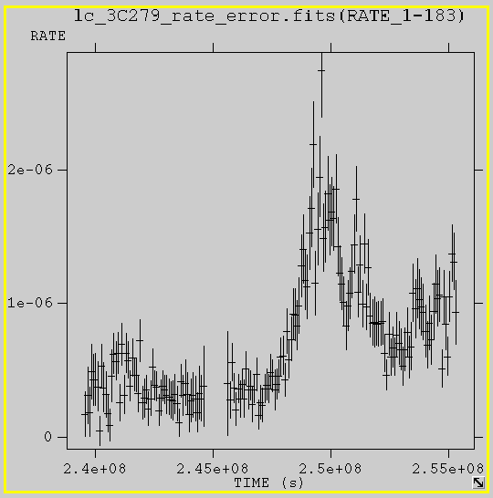 \n",
514 | "\n",
515 | "
\n",
514 | "\n",
515 | "