├── README.md
├── images
├── GSEA.png
├── GSEA02.png
├── HMM_01.png
├── MA_PLM.png
├── MA_RLE.png
├── MA_rma.png
├── MA_NUSE.png
├── MA_types.png
├── GSEA_Barbie.png
├── GSEA_ssGSEA.png
├── MA_GCprobes.png
├── MA_mapping.png
├── MA_oneColor.png
├── tcgsa
│ ├── clst3.png
│ ├── clust2.png
│ ├── baselineD1.png
│ ├── noBaseline.png
│ ├── hm_baseline.png
│ └── noBaseline_precluster.png
├── GSEA_Verhaak.png
├── MA_twoColors.png
├── intro
│ ├── ngsapps.png
│ ├── replicates.png
│ ├── wcm_schema.png
│ ├── replicates2.png
│ ├── AuerDoerge2010.png
│ └── biology-02-00378-g001.jpg
├── MA_medianPolish.png
├── nanopore_principle.png
├── MA_differentProbesets.png
├── nanopore_processing.png
├── nanopore_processing02.png
└── MA_normMethodComparison_TACmanual.png
├── references
└── GSEA
│ ├── lec14a.pdf
│ └── ssGSEA_caw_BIG_120314.pptx
├── RNA_heteroskedasticity_files
└── figure-html
│ ├── unnamed-chunk-3-1.png
│ ├── unnamed-chunk-5-1.png
│ ├── unnamed-chunk-8-1.png
│ ├── unnamed-chunk-9-1.png
│ └── unnamed-chunk-10-1.png
├── vdj_tcr_sequencing.md
├── bashrc
├── scRNA-seq_python
├── installing_scanpyEtc.sh
└── scRNA-seq_scanorama.Rmd
├── scRRBS.md
├── proteomics.md
├── shiny.md
├── integrativeAnalysis.md
├── alignment_vs_pseudoalignment.md
├── metabolomics.md
├── GOterm_overrepresentation.md
├── ExpHub_submission.md
├── hidden_markov_model.md
├── clusterProfiler_with_goseq.md
├── karyotype.md
├── rscript.md
├── dna_methylation.md
├── revigo.md
├── repeatMasker.md
├── scRNA-seq_RNAvelocity.md
├── Seurat_labelTransfer.md
├── spatial_transcriptomics.md
├── DimReds.md
├── atac.md
├── scRNA-seq_zinbwave_zinger.R
├── motif_analyses.md
├── nanopore_sequencing.md
├── repetitiveElements.md
├── scRNA-seq.md
├── Seurat.md
├── RNA_heteroskedasticity.md
├── RNA_heteroskedasticity.Rmd
├── CITE-seq.md
├── notes_10Q.md
├── IntroToNGS_WCMGS.md
└── microarrays.md
/README.md:
--------------------------------------------------------------------------------
1 | # Collection of notes about *omics analyses
2 |
--------------------------------------------------------------------------------
/images/GSEA.png:
--------------------------------------------------------------------------------
https://raw.githubusercontent.com/friedue/Notes/HEAD/images/GSEA.png
--------------------------------------------------------------------------------
/images/GSEA02.png:
--------------------------------------------------------------------------------
https://raw.githubusercontent.com/friedue/Notes/HEAD/images/GSEA02.png
--------------------------------------------------------------------------------
/images/HMM_01.png:
--------------------------------------------------------------------------------
https://raw.githubusercontent.com/friedue/Notes/HEAD/images/HMM_01.png
--------------------------------------------------------------------------------
/images/MA_PLM.png:
--------------------------------------------------------------------------------
https://raw.githubusercontent.com/friedue/Notes/HEAD/images/MA_PLM.png
--------------------------------------------------------------------------------
/images/MA_RLE.png:
--------------------------------------------------------------------------------
https://raw.githubusercontent.com/friedue/Notes/HEAD/images/MA_RLE.png
--------------------------------------------------------------------------------
/images/MA_rma.png:
--------------------------------------------------------------------------------
https://raw.githubusercontent.com/friedue/Notes/HEAD/images/MA_rma.png
--------------------------------------------------------------------------------
/images/MA_NUSE.png:
--------------------------------------------------------------------------------
https://raw.githubusercontent.com/friedue/Notes/HEAD/images/MA_NUSE.png
--------------------------------------------------------------------------------
/images/MA_types.png:
--------------------------------------------------------------------------------
https://raw.githubusercontent.com/friedue/Notes/HEAD/images/MA_types.png
--------------------------------------------------------------------------------
/images/GSEA_Barbie.png:
--------------------------------------------------------------------------------
https://raw.githubusercontent.com/friedue/Notes/HEAD/images/GSEA_Barbie.png
--------------------------------------------------------------------------------
/images/GSEA_ssGSEA.png:
--------------------------------------------------------------------------------
https://raw.githubusercontent.com/friedue/Notes/HEAD/images/GSEA_ssGSEA.png
--------------------------------------------------------------------------------
/images/MA_GCprobes.png:
--------------------------------------------------------------------------------
https://raw.githubusercontent.com/friedue/Notes/HEAD/images/MA_GCprobes.png
--------------------------------------------------------------------------------
/images/MA_mapping.png:
--------------------------------------------------------------------------------
https://raw.githubusercontent.com/friedue/Notes/HEAD/images/MA_mapping.png
--------------------------------------------------------------------------------
/images/MA_oneColor.png:
--------------------------------------------------------------------------------
https://raw.githubusercontent.com/friedue/Notes/HEAD/images/MA_oneColor.png
--------------------------------------------------------------------------------
/images/tcgsa/clst3.png:
--------------------------------------------------------------------------------
https://raw.githubusercontent.com/friedue/Notes/HEAD/images/tcgsa/clst3.png
--------------------------------------------------------------------------------
/images/GSEA_Verhaak.png:
--------------------------------------------------------------------------------
https://raw.githubusercontent.com/friedue/Notes/HEAD/images/GSEA_Verhaak.png
--------------------------------------------------------------------------------
/images/MA_twoColors.png:
--------------------------------------------------------------------------------
https://raw.githubusercontent.com/friedue/Notes/HEAD/images/MA_twoColors.png
--------------------------------------------------------------------------------
/images/intro/ngsapps.png:
--------------------------------------------------------------------------------
https://raw.githubusercontent.com/friedue/Notes/HEAD/images/intro/ngsapps.png
--------------------------------------------------------------------------------
/images/tcgsa/clust2.png:
--------------------------------------------------------------------------------
https://raw.githubusercontent.com/friedue/Notes/HEAD/images/tcgsa/clust2.png
--------------------------------------------------------------------------------
/images/MA_medianPolish.png:
--------------------------------------------------------------------------------
https://raw.githubusercontent.com/friedue/Notes/HEAD/images/MA_medianPolish.png
--------------------------------------------------------------------------------
/images/intro/replicates.png:
--------------------------------------------------------------------------------
https://raw.githubusercontent.com/friedue/Notes/HEAD/images/intro/replicates.png
--------------------------------------------------------------------------------
/images/intro/wcm_schema.png:
--------------------------------------------------------------------------------
https://raw.githubusercontent.com/friedue/Notes/HEAD/images/intro/wcm_schema.png
--------------------------------------------------------------------------------
/images/tcgsa/baselineD1.png:
--------------------------------------------------------------------------------
https://raw.githubusercontent.com/friedue/Notes/HEAD/images/tcgsa/baselineD1.png
--------------------------------------------------------------------------------
/images/tcgsa/noBaseline.png:
--------------------------------------------------------------------------------
https://raw.githubusercontent.com/friedue/Notes/HEAD/images/tcgsa/noBaseline.png
--------------------------------------------------------------------------------
/references/GSEA/lec14a.pdf:
--------------------------------------------------------------------------------
https://raw.githubusercontent.com/friedue/Notes/HEAD/references/GSEA/lec14a.pdf
--------------------------------------------------------------------------------
/images/intro/replicates2.png:
--------------------------------------------------------------------------------
https://raw.githubusercontent.com/friedue/Notes/HEAD/images/intro/replicates2.png
--------------------------------------------------------------------------------
/images/nanopore_principle.png:
--------------------------------------------------------------------------------
https://raw.githubusercontent.com/friedue/Notes/HEAD/images/nanopore_principle.png
--------------------------------------------------------------------------------
/images/tcgsa/hm_baseline.png:
--------------------------------------------------------------------------------
https://raw.githubusercontent.com/friedue/Notes/HEAD/images/tcgsa/hm_baseline.png
--------------------------------------------------------------------------------
/images/MA_differentProbesets.png:
--------------------------------------------------------------------------------
https://raw.githubusercontent.com/friedue/Notes/HEAD/images/MA_differentProbesets.png
--------------------------------------------------------------------------------
/images/intro/AuerDoerge2010.png:
--------------------------------------------------------------------------------
https://raw.githubusercontent.com/friedue/Notes/HEAD/images/intro/AuerDoerge2010.png
--------------------------------------------------------------------------------
/images/nanopore_processing.png:
--------------------------------------------------------------------------------
https://raw.githubusercontent.com/friedue/Notes/HEAD/images/nanopore_processing.png
--------------------------------------------------------------------------------
/images/nanopore_processing02.png:
--------------------------------------------------------------------------------
https://raw.githubusercontent.com/friedue/Notes/HEAD/images/nanopore_processing02.png
--------------------------------------------------------------------------------
/images/intro/biology-02-00378-g001.jpg:
--------------------------------------------------------------------------------
https://raw.githubusercontent.com/friedue/Notes/HEAD/images/intro/biology-02-00378-g001.jpg
--------------------------------------------------------------------------------
/images/tcgsa/noBaseline_precluster.png:
--------------------------------------------------------------------------------
https://raw.githubusercontent.com/friedue/Notes/HEAD/images/tcgsa/noBaseline_precluster.png
--------------------------------------------------------------------------------
/references/GSEA/ssGSEA_caw_BIG_120314.pptx:
--------------------------------------------------------------------------------
https://raw.githubusercontent.com/friedue/Notes/HEAD/references/GSEA/ssGSEA_caw_BIG_120314.pptx
--------------------------------------------------------------------------------
/images/MA_normMethodComparison_TACmanual.png:
--------------------------------------------------------------------------------
https://raw.githubusercontent.com/friedue/Notes/HEAD/images/MA_normMethodComparison_TACmanual.png
--------------------------------------------------------------------------------
/RNA_heteroskedasticity_files/figure-html/unnamed-chunk-3-1.png:
--------------------------------------------------------------------------------
https://raw.githubusercontent.com/friedue/Notes/HEAD/RNA_heteroskedasticity_files/figure-html/unnamed-chunk-3-1.png
--------------------------------------------------------------------------------
/RNA_heteroskedasticity_files/figure-html/unnamed-chunk-5-1.png:
--------------------------------------------------------------------------------
https://raw.githubusercontent.com/friedue/Notes/HEAD/RNA_heteroskedasticity_files/figure-html/unnamed-chunk-5-1.png
--------------------------------------------------------------------------------
/RNA_heteroskedasticity_files/figure-html/unnamed-chunk-8-1.png:
--------------------------------------------------------------------------------
https://raw.githubusercontent.com/friedue/Notes/HEAD/RNA_heteroskedasticity_files/figure-html/unnamed-chunk-8-1.png
--------------------------------------------------------------------------------
/RNA_heteroskedasticity_files/figure-html/unnamed-chunk-9-1.png:
--------------------------------------------------------------------------------
https://raw.githubusercontent.com/friedue/Notes/HEAD/RNA_heteroskedasticity_files/figure-html/unnamed-chunk-9-1.png
--------------------------------------------------------------------------------
/RNA_heteroskedasticity_files/figure-html/unnamed-chunk-10-1.png:
--------------------------------------------------------------------------------
https://raw.githubusercontent.com/friedue/Notes/HEAD/RNA_heteroskedasticity_files/figure-html/unnamed-chunk-10-1.png
--------------------------------------------------------------------------------
/vdj_tcr_sequencing.md:
--------------------------------------------------------------------------------
1 | VDJ/TCR sequencing
2 | ====================
3 |
4 | 
5 |
--------------------------------------------------------------------------------
/bashrc:
--------------------------------------------------------------------------------
1 | ```sh
2 | # .bashrc
3 |
4 | # Source global definitions
5 | #if [ -f /etc/bashrc ]; then
6 | # . /etc/bashrc
7 | #fi
8 |
9 | # User specific aliases and functions
10 |
11 | alias ls='ls -lahFG'
12 | export LC_NUMERIC=en_US.UTF-8
13 | export LC_ALL=en_US.UTF-8
14 |
15 | # This makes the system reluctant to wipe out existing files via cp and mv
16 | set -o noclobber
17 | ```
18 |
--------------------------------------------------------------------------------
/scRNA-seq_python/installing_scanpyEtc.sh:
--------------------------------------------------------------------------------
1 |
2 | # combining anaconda & pip: https://www.anaconda.com/using-pip-in-a-conda-environment/
3 | conda search scanpy
4 | conda info --envs
5 | conda activate scrna # make sure to switch to that environment
6 | conda install pip
7 | /scratchLocal/frd2007/software/anaconda3/envs/scrna/bin/pip install scanorama
8 |
9 | ## testing scanorama
10 | wget https://raw.githubusercontent.com/brianhie/scanorama/master/bin/process.py --no-check-certificate
11 |
12 |
13 |
14 |
--------------------------------------------------------------------------------
/scRRBS.md:
--------------------------------------------------------------------------------
1 | scRRBS
2 | ============
3 |
4 | * original paper: [Guo et al.](https://www.ncbi.nlm.nih.gov/pubmed/24179143)
5 |
6 | * general pros/cons of RRBS apply:
7 | * low coverage of regions with little CpG density
8 | * generally sparse representation: ca. 1 mio CpGsv(1-10% of all CpGs)
9 | * improved detection of promoter/CpG-rich regions
10 | * relatively consistent across replicates
11 |
12 |
13 | [DeepCpG](https://github.com/PMBio/deepcpg/blob/master/examples/README.md) can be used to impute missing values to get a more granular picture at the single-cell level
14 | [Angermueller et al., 2017](https://genomebiology.biomedcentral.com/articles/10.1186/s13059-017-1189-z#Abs1)
--------------------------------------------------------------------------------
/proteomics.md:
--------------------------------------------------------------------------------
1 | Proteomics
2 | ===========
3 |
4 | | Score | Meaning | Reference |
5 | |--------|---------|-----------|
6 | | Ascore | localization of a phosphorylation site; score is the difference between the top scorer - 2nd best scorer | [Ascore][Ascore] |
7 | | Maxscore | | |
8 | | Modscore | modscore is an updated version of Ascore | |
9 | | Localization score | | |
10 |
11 | - `#` missing TMT label
12 | - `]` missing TMT label at N-terminus
13 | - `@` lysine
14 | - `@]@` glitch
15 |
16 | References for the Gygi lab pipeline:
17 |
18 | * [Mouse Phospho-Proteomics Atlas][Mouse Atlas]
19 | * [Ascore][Ascore]
20 |
21 |
22 |
23 |
24 |
25 | [Ascore]: https://www.ncbi.nlm.nih.gov/pubmed/21183079 "Huttlin et al., Cell (2010)"
26 | [Mouse Atlas]: http://ascore.med.harvard.edu/ "Ascore"
27 |
--------------------------------------------------------------------------------
/shiny.md:
--------------------------------------------------------------------------------
1 |
2 | Why shiny apps tend to become unwieldy quickly:
3 |
4 | >Input and output IDs in Shiny apps share a global namespace, meaning, each ID must be unique across the entire app. If you’re using functions to generate UI, and those functions generate inputs and outputs, then you need to ensure that none of the IDs collide. [1][1]
5 |
6 | ## Shiny modules
7 |
8 | * piece of a Shiny app
9 | * can’t be directly run
10 | * included as part of a larger app (or as part of a larger Shiny module–they are composable)
11 | * add namespacing to Shiny UI and server logic
12 |
13 | Modules can represent input, output, or both.
14 |
15 | * composed of two functions that represent 1) a piece of UI, and 2) a fragment of server logic that uses that UI
16 |
17 | ---------------
18 | [1]: https://shiny.rstudio.com/articles/modules.html
19 |
--------------------------------------------------------------------------------
/integrativeAnalysis.md:
--------------------------------------------------------------------------------
1 | Integrative analyses
2 | ---------------------
3 |
4 | * [Review of methods](http://insights.sagepub.com/redirect_file.php?fileId=6771&filename=5060-BMI-Genomic,-Proteomic,-and-Metabolomic-Data-Integration-Strategies.pdf&fileType=pdf) and introduction to the Grinn R package (predecessor to Metabobox)
5 |
6 | ### Metabobox (R package, 2017)
7 |
8 | - see Metabolomics Notes
9 | - [github repo](https://github.com/kwanjeeraw/mETABOX)
10 |
11 | ### __3omics__ (not updated since 2012)
12 | - has a Name-ID converter
13 | - [Example data](http://3omics.cmdm.tw/help.php#examples) and analysis details
14 | - Correlation Network
15 | - "3Omics generates inter-omic correlation network to display the relationship or common patterns in data over time or experimental conditions for all transcripts, proteins and metabolites. Where users may only have two of the three -omics data-sets, 3Omics supplements the missing transcript, protein or metabolite information by searching iHOP"
16 | - Coexpression Profile
17 | - Phenotype Analysis
18 | - Pathway Analysis
19 | - GO Enrichment Analysis
--------------------------------------------------------------------------------
/alignment_vs_pseudoalignment.md:
--------------------------------------------------------------------------------
1 | Rob Patro:
2 |
3 | >Selective alignment is simply an efficient mechanism to compute actual alignment scores, it performs sensitive seeding, seed chaining & scoring, and crucially, actually computes an alignment score (via DP), while pseudo-alignment does not do these things, and is a way to quickly determine the likely compatibility between a read and a set of references.
4 |
5 | > Both of the approaches are algorithmic ways to return, in the case of pseudoalignment, sets of references [that are most compatible with the reads at hand],
6 | and in the case of selective alignment, scored mappings. They can both be run over "arbitrary" referenced indices.
7 |
8 | >If you don't (1) validate the "compatibility" you find and (2) seed in a sensitive fashion, then you end up with mappings whose accuracy is lesser than that derived from alignments. [see their pre-print on this](https://www.biorxiv.org/content/10.1101/657874v1)
9 |
10 | > For example, a 100bp read could "pseudoalign" to a transcript with which it shares only a single k-mer although that would preclude any reasonable quality alignment. There is no scoring adopted in the determination of compatibility, which can and does lead to spurious mapping.
11 |
--------------------------------------------------------------------------------
/metabolomics.md:
--------------------------------------------------------------------------------
1 | Metabolomics
2 | ---------------
3 |
4 | ### Metabobox (2017)
5 |
6 | - R package, [paper](http://journals.plos.org/plosone/article?id=10.1371/journal.pone.0171046)
7 | - can probably be used with other data types, too
8 | - [github repo](https://github.com/kwanjeeraw/mETABOX)
9 | - features:
10 | - Data normalization and data transformation
11 | - Univariate statistical analyses with hypothesis testing procedures that are automatically selected based on study designs
12 | - Joint and interactive visualization of genes, proteins and metabolites in different combinations of networks
13 | - Calculation of data-driven networks using correlation-based approaches
14 | - Calculation of chemical structure similarity networks from substructure fingerprints
15 | - Functional interpretation with overrepresentation analysis, functional class scoring and WordCloud generation
16 |
17 | 
18 |
19 | #### Network analysis
20 |
21 | * internal graph database: a _pre-compiled graph database_, which is used for collecting prior knowledge from several [resources](http://journals.plos.org/plosone/article/file?id=10.1371/journal.pone.0171046.s001&type=supplementary) (Note: based on GRCh38 (!))
22 |
23 |
24 |
--------------------------------------------------------------------------------
/GOterm_overrepresentation.md:
--------------------------------------------------------------------------------
1 | ## ClusterProfiler
2 |
3 | * `enrichGO` and `enrichKEGG`: test based on hypergeometric distribution with additional multiple hypothesis-testing correction [Paper](https://www.liebertpub.com/doi/10.1089/omi.2011.0118)
4 |
5 | ```
6 | ## retrieve ENTREZ IDs
7 | eg <- clusterProfiler::bitr(t_tx$gene_symbol, fromType="SYMBOL", toType="ENTREZID", OrgDb="org.Hs.eg.db") %>%
8 | as.data.table
9 | setnames(eg, names(eg), c("gene_symbol", "entrez"))
10 |
11 | clstcomp <- eg[t_tx, on = "gene_symbol"] %>%
12 | .[, c("gene_symbol","entrez","cluster_k60","day","logFC"), with=FALSE] %>%
13 | .[!is.na(entrez)] %>% unique
14 |
15 | ## make a list of ENTREZ IDs, one per cluster
16 | clstcomp.list <- lapply(sort(unique(clstcomp$cluster_k60)), function(x) clstcomp[cluster_k60 == x]$entrez )
17 |
18 | ## run enrichGO
19 | ck.GO_bp <- compareCluster(clstcomp.list, fun = "enrichGO", OrgDb = org.Hs.eg.db, ont = "BP")
20 |
21 | ## visualization
22 | dotplot(ck.GO_bp) + ggtitle("Overrepresented GO terms (Biological Processes)")
23 |
24 | ```
25 |
26 | Individual lists (no comparisons)
27 |
28 | ```
29 | cp.GO_bp.ind <- lapply(clstcomp.list, function(x){
30 | out <- enrichGO(x, OrgDb = org.Mm.eg.db, universe = unique(deg.dt$entrez), ont = "BP", pvalueCutoff = 0.05, pAdjustMethod = "BH")
31 | out <- DOSE::setReadable(out, 'org.Mm.eg.db', 'ENTREZID')
32 | return(out)
33 | })
34 | ```
35 |
36 | * `geneRatio` should be number of genes that overlap gene set divided by size of gene set
37 | * the number in parentheses for the clusterCompare plot corresponds to the number of genes that were in that group
38 |
--------------------------------------------------------------------------------
/ExpHub_submission.md:
--------------------------------------------------------------------------------
1 | For **every data set**:
2 |
3 | ## 1. Save data and metadata in ExpHub (documentation by [ExperimentHub](https://bioconductor.org/packages/3.10/bioc/vignettes/ExperimentHub/inst/doc/CreateAnExperimentHubPackage.html))
4 | - .R or .Rmds stored in `inst/scripts/`
5 | - `make-data.Rmd` -- describe how the data stored in ExpHub was obtained and saved. [example Rmd](https://github.com/LTLA/scRNAseq/blob/master/inst/scripts/make-nestorowa-hsc-data.Rmd)
6 | ```
7 | ## describe how the data was obtained and processed
8 | count.file <- read.table("file.txt")
9 | counts <- as.matrix(count.file)
10 | coldata <- DataFrame(row.names = colnames(count.file),
11 | condition = c("A","A","B","B"))
12 |
13 | ## save the data
14 | path <- file.path("myPackage", "storeddata", "1.0.0")
15 | dir.create(path, showWarnings-FALSE, recursive=TRUE)
16 |
17 | saveRDS(counts, file = file.path(path, "counts.rds"))
18 | saveRDS(coldata, file = file.path(path, "coldata.rds"))
19 | ```
20 | - `make-metadata.R` -- generate a csv file that will be stored in the `inst/extdata` folder of the package, the result can look [like this](https://github.com/LTLA/scRNAseq/blob/master/inst/extdata/metadata-nestorowa-hsc.csv). [example R script](https://github.com/LTLA/scRNAseq/blob/master/inst/scripts/make-nestorowa-hsc-metadata.R)
21 | ```
22 | write.csv(file = "../extdata/metadata-storeddata.csv", stringsAsFactors = FALSE, data.frame(...) )
23 | ```
24 | ## 2. Provide functions to generate the R object that will be exposed to the user
25 | - scripts in `R/`
26 | - `get_storeddata.R`
27 | ```
28 | get_data_hpca <- function() {
29 | version <- "1.0.0"
30 | se <- .create_se(file.path("hpca", version), has.rowdata=FALSE)
31 | }
32 | ```
33 | - `create_se.R`
34 |
--------------------------------------------------------------------------------
/hidden_markov_model.md:
--------------------------------------------------------------------------------
1 | ## Hidden Markov Model
2 |
3 | from [[1]]():
4 |
5 | Each state has its own __emission probabilities__, which, for example, models the base composition of exons, introns and the consensus G at the 5′SS.
6 |
7 | Each state also has __transition probabilities__, the probabilities of moving from this state to a new state.
8 |
9 | 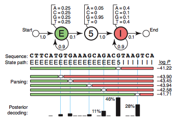
10 |
11 | [Casino example](http://learninglover.com/blog/?p=635)
12 |
13 | ### Baum-Welch algorithm
14 |
15 | The Baum–Welch algorithm is used to find the unknown parameters of a hidden Markov model (HMM). [[2]] I.e. given a sequence of observations, generate a transition and emission matrix that may have generated the observations. [[4]]
16 |
17 | The BWA makes use of the forward-backward algorithm. [[2]]
18 |
19 |
20 |
21 | ### Viterbi path
22 |
23 | There are potentially many state paths that could generate the same sequence. We want to find the one with the highest probability. (...) The efficient Viterbi algorithm is guaranteed to find the most probable state path given a sequence and an HMM. [[1]]
24 | The Baum–Welch algorithm uses the well known EM algorithm to find the maximum likelihood estimate of the parameters of a hidden Markov model given a set of observed feature vectors. [[3]]
25 |
26 | HMMs don’t deal well with correlations between residues, because they assume that each residue depends only on one underlying state. [[1]]
27 |
28 | [interactive spreasheet for teaching forward-backward algorithm](http://www.cs.jhu.edu/~jason/papers/#eisner-2002-tnlp)
29 |
30 |
31 | ----------------------
32 | [1]: http://dx.doi.org/10.1038/nbt1004-1315 "Eddy, S. Nat Biotech (2014)"
33 | [2]: https://en.wikipedia.org/wiki/Baum%E2%80%93Welch_algorithm "Wikipedia: Baum Welch algorithm]"
34 | [3]: https://en.wikipedia.org/wiki/Viterbi_algorithm "Wikipedia: Viterbi algorithm"
35 | [4]: http://biostat.jhsph.edu/bstcourse/bio638/readings/BW.pdf "Baum-Welch Algorithm explained"
36 |
--------------------------------------------------------------------------------
/clusterProfiler_with_goseq.md:
--------------------------------------------------------------------------------
1 | I've been perpetually annoyed by the fact that clusterProfiler offers useful visualizations, but I don't want to miss out on the correction that GOseq offers.
2 | So, here's a way to combine them both by replacing the p-values of the clusterProfiler result with the goseq results.
3 | It would probably make sense to use no cut-off when running enrichGO to obtain all possible gene sets.
4 |
5 | ```
6 | # GOSEQ =================
7 | library(goseq) # package for GO term enrichment that also accounts for gene legnth
8 | gene.vector <- row.names(DGE.results) %in% DGEgenes %>% as.integer
9 | names(gene.vector) <- row.names(DGE.results)
10 | pwf <- nullp(gene.vector, "sacCer3", "ensGene")
11 | GO.wall <- goseq(pwf, "sacCer3", "ensGene")
12 |
13 | # CLUSTERPROFILE=========
14 | library(clusterProfiler)
15 | dge <- subset(dgeres, padj <= 0.01 )$ENTREZID
16 | go_enrich <- enrichGO(gene = dge,
17 | universe = dgeres$ENTREZID,
18 | OrgDb = "org.Sc.sgd.db",
19 | keyType = 'ENTREZID',
20 | readable = F, # setting this TRUE won't work with yeast
21 | ont = "BP",
22 | pvalueCutoff = 0.05, # probably better to turn this off
23 | qvalueCutoff = 0.10)
24 |
25 | # COMBINE =================
26 |
27 | comp.go <- merge(go_enrich@result[,1:7], GO.wall,
28 | by.x = "ID", by.y = "category", all = TRUE)
29 |
30 | ## get adjusted goseq p.values
31 | comp.go$padj_for_cp <- p.adjust(comp.go$pvalue, method = "BH") # BH is the default choice in enrichGO
32 |
33 | ## before we replace, we need to make sure that our df matches the results of enrichGO
34 | rownames(comp.go) <- comp.go$ID
35 | comp.go <- subset(comp.go, !is.na(pvalue))
36 | comp.go <- comp.go[rownames(go_enrich@result),]
37 |
38 | ## add the goseq-values to the enrichGO results
39 | go.res <- go_enrich
40 | go.res@result$p.adjust <- comp.go$padj_for_cp
41 | go.res@result$pvalue <- comp.go$over_represented_pvalue
42 |
43 | # TADAA
44 | dotplot(go.res, showCategory = 10)
45 | ````
--------------------------------------------------------------------------------
/karyotype.md:
--------------------------------------------------------------------------------
1 | ## Karyotype plots
2 |
3 | - Cytogenetic G-banding data (G-banding = Giemsa staining based)
4 | - Giemsa bands are related to functional nuclear processes such as replication or transcription in the following points
5 | - G bands are late- replicating
6 | - chromatins in G bands are more condensed
7 | - G-band DNA is localized at the nuclear periphery
8 | - G bands are homoge- neous in GC content and essentially consist of GC-poor iso- chores
9 |
10 | [PNAS 2002](doi.dx.org/10.1073/pnas.022437999)
11 |
12 | Recommended package: [karyoploteR](https://bernatgel.github.io/karyoploter_tutorial/) ([vignette](https://bioconductor.org/packages/release/bioc/vignettes/karyoploteR/inst/doc/karyoploteR.html))
13 |
14 | 
15 |
16 | >Chemically staining the metaphase chromosomes results in a alternating dark and light banding pattern, which could provide information about abnormalities for chromosomes. Cytogenetic bands could also provide potential predictions of chromosomal structural characteristics, such as repeat structure content, CpG island density, gene density, and GC content.
17 | biovizBase package provides utilities to get ideograms from the UCSC genome browser, as a wrapper around some functionality from rtracklayer. It gets the table for cytoBand and stores the table for certain species as a GRanges object.
18 | We found a color setting scheme in package geneplotter, and we implemented it in biovisBase.
19 | The function .cytobandColor will return a default color set. You could also get it from options after you load biovizBase package.
20 | And we recommended function getBioColor to get the color vector you want, and names of the color is biological categorical data. This function hides interval color genenerators and also the complexity of getting color from options. You could specify whether you want to get colors by default or from options, in this way, you can temporarily edit colors in options and could change or all the graphics. This give graphics a uniform color scheme.
21 |
22 | [BioViz Vignette](https://www.bioconductor.org/packages/release/bioc/vignettes/biovizBase/inst/doc/intro.pdf)
23 |
24 | - brown/red corresponds to "stalk"
25 |
--------------------------------------------------------------------------------
/rscript.md:
--------------------------------------------------------------------------------
1 | # Basic use of `Rscript`
2 |
3 | Example script content:
4 |
5 | ```
6 | #!/usr/bin/env Rscript
7 | args <- commandArgs(trailingOnly = TRUE)
8 | rnorm(n=as.numeric(args[1]), mean=as.numeric(args[2]))
9 | ```
10 |
11 | Invoke the script:
12 |
13 | ```
14 | $ Rscript myScript.R 5 100
15 | ```
16 |
17 | Obviously, this creates a string vector `args` which contains the entries `5` and `100`
18 |
19 | General usage:
20 |
21 | ```
22 | Rscript [options] [-e expr [-e expr2 ...] | file] [args]
23 | ```
24 |
25 | Handling mising arguments:
26 |
27 | ```
28 | # test if there is at least one argument: if not, return an error
29 | if (length(args)==0) {
30 | stop("At least one argument must be supplied (input file).n", call.=FALSE)
31 | } else if (length(args)==1) {
32 | # default output file
33 | args[2] = "out.txt"
34 | }
35 | ```
36 |
37 | For storing helpful information about what types of parameters are expected etc., the `optparse` package is the way to go. [Eric Minikel](https://gist.github.com/ericminikel/8428297) has a great example. Below is a shorter summary:
38 |
39 | ```
40 | #!/usr/bin/env Rscript
41 | library("optparse")
42 |
43 | option_list = list(
44 | make_option(c("-f", "--file"), type="character", default=NULL,
45 | help="dataset file name", metavar="character"),
46 | make_option(c("-o", "--out"), type="character", default="out.txt",
47 | help="output file name [default= %default]", metavar="character")
48 | );
49 |
50 | opt_parser = OptionParser(option_list=option_list);
51 | opt = parse_args(opt_parser); # list with all the arguments sorted by order of appearance in option_list
52 | ```
53 |
54 | Arguments can be called by their names; here: `opt$file` and `opt$out`:
55 |
56 | ```
57 | ## program...
58 | df = read.table(opt$file, header=TRUE)
59 | num_vars = which(sapply(df, class)=="numeric")
60 | df_out = df[ ,num_vars]
61 | write.table(df_out, file=opt$out, row.names=FALSE)
62 | ```
63 |
64 | ## References
65 |
66 | -
67 | -
68 | -
69 | - [Great presentation touching on all important points](https://nbisweden.github.io/RaukR-2018/working_with_scripts_Markus/presentation/WorkingWithScriptsPresentation.html#1)
70 |
--------------------------------------------------------------------------------
/dna_methylation.md:
--------------------------------------------------------------------------------
1 | * [DNA methylation basics](#basics)
2 | * [Regions defined by DNA methylation](#regions)
3 |
4 | -------------------------------
5 |
6 |
7 | ## DNA methylation basics
8 |
9 | see [Messerschmidt Review (2014)]
10 |
11 | * undetectable in certain yeast, nematode, and fly species
12 | * in mamamals, DNA methylation is vital
13 | * mostly in __symmetrical CpG context__
14 | * single CpGs typically hypermethylated vs. unmethylated CpG islands --> __low CpG density promoters__ are generally hypermethylated, yet active vs. __high CpG density promoters__ that are inactive if methylated
15 | * __transposons__ are repressed if methylated (esp. LINEs, LTRs), so are __pericentromeric repeats__
16 | * __imprinted genes__ show parent-of-origin-specific DNA methylation (introduced during gamete differentiation) and subsequently allele-specific gene expression
17 |
18 | ### DNA methylation machinery
19 |
20 | #### _de novo_ methylation
21 |
22 | --> __Dnmt3a, Dnmt3b__
23 |
24 | * maternally provided (Dnmt3a)
25 |
26 | #### methylation maintenance
27 |
28 | --> __Dnmt1__
29 |
30 | * high affinity for hemimethylation
31 | * its deletion in mESCs causes hypotmethylation, but not a complete loss (lethal effect, though)
32 |
33 | _Dnmt2_ is a misnomer: it methylates RNA, not DNA
34 |
35 |
36 | ## Regions defined by DNA methylation
37 |
38 | | |LMR|UMR|IMR|PMD|
39 | |-|---|---|---|---|
40 | |me level| 10-50% | 0-10% |mean: 57% | 0-100%, seemingly disordered|
41 | |size|||271 bp| 150 kb|
42 | |abundance||||20-40% of the genome|
43 | |tissue-specific?|yes||yes, mostly| yes (not present in ESC)|
44 | |CpG content|low|high|not defined|variable|
45 | |localization|DHS overlap|mostly promoters, CGIs|mostly intragenic|heterochromatin|
46 | |reference|[Stadler (2011)]()|[Stadler (2011)]()|[Elliott (2015)]()|[Lister (2009)](), [Gaidatzis (2014)]()|
47 |
48 |
49 | -------------
50 | [Elliott (2015)]: http://dx.doi.org/10.1038/ncomms7363 "Elliott et al., Nat Comms (2015): Intermediate DNA methylation is a conserved signature of genome regulation"
51 | [Lister (2009)]: http://dx.doi.org/10.1038/nature08514 "Lister et al., Nature (2009): Human DNA methylomes at base resolution show widespread epigenomic differences"
52 | [Messerschmidt Review (2014)]:http://dx.doi.org/10.1101/gad.234294.113 "Messerschmidt et al., Genes & Development (2014): DNA methylation dynamics during epigenetic reprogramming in the germline and preimplantation embryos"
53 | [Stadler (2011)]:http://dx.doi.org/10.1038/nature11086 "Stadler et al., Nature (2011): DNA-binding factors shape the mouse methylome at distal regulatory regions"
54 |
55 |
--------------------------------------------------------------------------------
/revigo.md:
--------------------------------------------------------------------------------
1 | # Summarizing GO terms using semantic similarity
2 |
3 | [REVIGO](http://revigo.irb.hr/) clusters GO terms based on their semantic similarity, p-values, and relatedness resulting in a hierarchical clustering where less dispensable terms are placed closer to the root. The clustering is visualized in a clustered heatmap showing the p-values for each term.
4 |
5 | REVIGO generates multiple plots; the easiest way to obtain them in high quality is to download the R scripts that it offers underneath each of the options (e.g. scatter plot, tree map) and to run those yourself.
6 |
7 | Here, I've downloaded the R script after selecting the treemap plot ("Make R script for plotting").
8 | The script is aptly named `REVIGO_treemap.r`.
9 | The plot can be generated as easily as this:
10 |
11 | ```{r eval=FALSE}
12 | ## this will generate a PDF file named "REVIGO_treemap.pdf" in your current
13 | ## working directory
14 | source("~/Downloads/REVIGO_treemap.r")
15 | ```
16 |
17 | Since I personally don't like plots being immediately printed to PDF (much more difficult to include them in an Rmarkdown!),
18 | I've tweaked the function a bit; it's essentially the original REVIGO script that I downloaded minus the part where the `revigo.data` object is generated and with a couple more options to tune the resulting heatmap.
19 |
20 | ```{r define_own_treemap_function}
21 | REVIGO_treemap <- function(revigo.data, col_palette = "Paired",
22 | title = "REVIGO Gene Ontology treemap", ...){
23 | stuff <- data.frame(revigo.data)
24 | names(stuff) <- c("term_ID","description","freqInDbPercent","abslog10pvalue",
25 | "uniqueness","dispensability","representative")
26 | stuff$abslog10pvalue <- as.numeric( as.character(stuff$abslog10pvalue) )
27 | stuff$freqInDbPercent <- as.numeric( as.character(stuff$freqInDbPercent) )
28 | stuff$uniqueness <- as.numeric( as.character(stuff$uniqueness) )
29 | stuff$dispensability <- as.numeric( as.character(stuff$dispensability) )
30 | # check the treemap command documentation for all possible parameters -
31 | # there are a lot more
32 | treemap::treemap(
33 | stuff,
34 | index = c("representative","description"),
35 | vSize = "abslog10pvalue",
36 | type = "categorical",
37 | vColor = "representative",
38 | title = title,
39 | inflate.labels = FALSE,
40 | lowerbound.cex.labels = 0,
41 | bg.labels = 255,
42 | position.legend = "none",
43 | fontsize.title = 22, fontsize.labels=c(18,12,8),
44 | palette= col_palette, ...
45 | )
46 | }
47 | ```
48 |
49 | I still need the originally downloaded script to generate the `revigo.data` object, which I will then pass onto my newly tweaked function.
50 | Using the command line (!) tools `sed` and `egrep`, I'm going to only keep the lines between the one starting with "revigo.data" and the line starting with "stuff".
51 | The output of that will be parsed into a new file, which will only generate the `revigo.data` object that I'm after (no PDF!).
52 |
53 | ```{r}
54 | # the system function allows me to run command line stuff outside of R
55 | # just for legibility purposes, I'll break up the command into individual
56 | # components, which I'll join back together using paste()
57 | sed_cmd <- "sed -n '/^revigo\\.data.*/,/^stuff.*/p'"
58 | fname <- "~/Downloads/REVIGO_treemap.r"
59 | egrep_cmd <- "egrep '^rev|^c'"
60 | out_fname <- "~/Downloads/REVIGO_myData.r"
61 | system(paste(sed_cmd, fname, "|", egrep_cmd, ">", out_fname))
62 | ## upon sourcing; no treemap PDF will be generated, but the revigo.data object
63 | ## should appear in your R environment
64 | source("~/Downloads/REVIGO_myData.r")
65 | REVIGO_treemap(revigo.data)
66 | ```
67 |
68 | If this is all too tedious, you may want to check out a recent Python implementation of REVIGO's principles: [GO-figure](https://www.biorxiv.org/content/10.1101/2020.12.02.408534v1.full).
--------------------------------------------------------------------------------
/repeatMasker.md:
--------------------------------------------------------------------------------
1 | Understanding repeatMasker and repeat annotation
2 | ==================================================
3 |
4 | >RepeatMasker is a program that screens DNA sequences for interspersed repeats and low complexity DNA sequences. The output of the program is a detailed annotation of the repeats that are present in the query sequence as well as a modified version of the query sequence in which all the annotated repeats have been masked
5 |
6 | From:
7 |
8 | Repeats are identified with `RepeatModeler`.
9 |
10 | The full repeatMasker track can be downloaded e.g. via `wget "https://hgdownload.soe.ucsc.edu/goldenPath/mm10/database/rmsk.txt.gz"`
11 | The fields should be labelled as follows:
12 |
13 | | Field | Meaning |
14 | |-------|---------|
15 | | chrom | "Genomic sequence name" |
16 | | chromStart | "Start in genomic sequence" |
17 | | chromEnd | "End in genomic sequence" |
18 | | name | "Name of repeat"|
19 | | score | "always 0 place holder"|
20 | | strand | "Relative orientation + or -"|
21 | | swScore | "Smith Waterman alignment score"|
22 | | milliDiv| "Base mismatches in parts per thousand"|
23 | |milliDel | "Bases deleted in parts per thousand"|
24 | | milliIns | "Bases inserted in parts per thousand"|
25 | | genoLeft | "-#bases after match in genomic sequence"|
26 | | repClass | "Class of repeat"|
27 | |repFamily | "Family of repeat"|
28 | |repStart| "Start (if strand is +) or -#bases after match (if strand is -) in repeat sequence"|
29 | | repEnd| "End in repeat sequence"|
30 | | repLeft| "-#bases after match (if strand is +) or start (if strand is -) in repeat sequence"|
31 |
32 | Based on info from
33 |
34 | * up to ten different **classes** of repeats:
35 | * Short interspersed nuclear elements (SINE), which include ALUs
36 | * Long interspersed nuclear elements (LINE)
37 | * Long terminal repeat elements (LTR), which include retroposons
38 | * DNA repeat elements (DNA)
39 | * Simple repeats (micro-satellites)
40 | * Low complexity repeats
41 | * Satellite repeats
42 | * RNA repeats (including RNA, tRNA, rRNA, snRNA, scRNA, srpRNA)
43 | * Other repeats, which includes class RC (Rolling Circle)
44 | * Unknown
45 |
46 | "A "?" at the end of the "Family" or "Class" (for example, DNA?) signifies that the curator was unsure of the classification. At some point in the future, either the "?" will be removed or the classification will be changed."
47 |
48 | from [UCSC GenomeBrowser Track description](https://genome.ucsc.edu/cgi-bin/hgTables?db=hg19&hgta_group=rep&hgta_track=rmsk&hgta_table=rmsk&hgta_doSchema=describe+table+schema)
49 |
50 | ## Families, classes and so on
51 |
52 | >The most elementary level of classification of TEs is the family, which designates interspersed genomic copies derived from the amplification of an ancestral progenitor sequence (10). Each TE family can be represented by a consensus sequence approximating that of the ancestral progenitor.
53 |
54 | From [Flynn et al. (2020)](https://www.ncbi.nlm.nih.gov/pmc/articles/PMC7196820/)
55 |
56 | >RepeatModeler contains a basic homology-based classification module (RepeatClassifier) which compares the TE families generated by the various de novo tools to both the RepeatMasker Repeat Protein Database (DB) and to the RepeatMasker libraries (e.g., Dfam and/or RepBase). The Repeat Protein DB is a set of TE-derived coding sequences that covers a wide range of TE classes and organisms. As is often the case with a search against all known TE consensus sequences, there will be a high number of false positive or partial matches. RepeatClassifier uses a combination of score and overlap filters to produce a reduced set of high-confidence results. If there is a concordance in classification among the filtered results, RepeatClassifier will label the family using the RepeatMasker/Dfam classification system and adjust the orientation (if necessary). Remaining families are labeled “Unknown” if a call cannot be made. Classification is the only step that requires a database, and can be completed with only open-source Dfam if Repbase is not available.
57 |
--------------------------------------------------------------------------------
/scRNA-seq_RNAvelocity.md:
--------------------------------------------------------------------------------
1 | # RNA velocity
2 |
3 | ## Basics
4 |
5 | * Goal: **predict the future expression state of a cell**
6 | * input: two gene-by-cell matrices
7 | * one with spliced (`S`)
8 | * one with unspliced counts (`U`)
9 |
10 | For each *gene*, a phase-plot is constructed.
11 | That phase-plot is used to estimate the gene- and cell-specific velocity.
12 | The phase-plot is a scatterplot of the relevant row (gene) from the U and S matrices (well, a moment estimator of these quantities, but that is a minor point). In other words, the gene-specific velocities are determined by the relationship of S and U. [(HansenLabBlog)](http://www.hansenlab.org/velocity_batch)
13 |
14 | In the words of the Theis Lab:
15 | >For each gene, a steady-state-ratio of pre-mature (unspliced) and mature (spliced) mRNA counts is fitted, which constitutes a constant transcriptional state. Velocities are then obtained as **residuals from this ratio**. Positive velocity indicates that a gene is up-regulated, which occurs for cells that show higher abundance of unspliced mRNA for that gene than expected in steady state. Conversely, negative velocity indicates that a gene is down-regulated.
16 |
17 | [This gif](https://user-images.githubusercontent.com/31883718/80227452-eb822480-864d-11ea-9399-56886c5e2785.gif) illustrates the principles.
18 |
19 | In brief, velocity is estimated for each gene in each cell and then projected into lower dimensional space to reveal the direction of *cell* fate transitions.
20 | The extraplolation of traditional RNA velocity measurements is valid for approx. a couple of hours (based on [Qiu et al., 2022](https://doi.org/10.1016/j.cell.2021.12.045).
21 |
22 | ### Batch effect
23 |
24 | Batch effect seems to be present according to the Hansen Lab. [(HansenLabBlog)](http://www.hansenlab.org/velocity_batch)
25 |
26 | Challenge for RNA velocity: we need to batch correct not 1 but 2 matrices simultaneously
27 |
28 | `scVelo` currently does not pay attention to this, as they state "any additional preprocessing step only affects X and is not applied to spliced/unspliced counts." [(Ref)](https://colab.research.google.com/github/theislab/scvelo_notebooks/blob/master/VelocityBasics.ipynb#scrollTo=SgjdS1emFTbq)
29 |
30 | HansenLab suggests:
31 |
32 | >we correct S and U for library size, and form M=U+S. Then we log-transform M as log(M+1), use ComBat and invert the log transformation. This is what we feed to scVelo and friends. [Details](http://www.hansenlab.org/velocity_batch)
33 |
34 | ## Processing details
35 |
36 | The starting point for any type of velocity analysis: **2 count matrices of pre-mature (unspliced) and mature (spliced) abundances**.
37 |
38 | These can be obtained from standard sequencing protocols, using the `velocyto.py` or `loompy/kallisto` counting pipeline.
39 |
40 | [**Velocyto**](http://velocyto.org/velocyto.py/tutorial/index.html) offers multiple wrappers around 10X Genomics (CellRanger) data, Smart-seq2 data etc.
41 | It essentially looks at every single mapped read and determines whether it represents a spliced, unspliced or ambiguous molecule.
42 |
43 | The BAM file will have to:
44 |
45 | - Be sorted by mapping position.
46 | - Represents either a single sample (multiple cells prepared using a certain barcode set in a single experiment) or single cell.
47 | - Contain an error corrected cell barcodes as a TAG named CB or XC.
48 | - Contain an error corrected molecular barcodes as a TAG named UB or XM.
49 |
50 | ```
51 | # wrapper for 10X
52 | velocyto run10x -m repeat_msk.gtf mypath/sample01 somepath/refdata-cellranger-mm10-1.2.0/genes/genes.gtf
53 |
54 | # same thing with the simple velocyto run command
55 | velocyto run -b filtered_barcodes.tsv -o output_path -m repeat_msk_srt.gtf bam_file.bam annotation.gtf
56 | ```
57 |
58 | The output is a 4-layered [loom file](http://linnarssonlab.org/loompy/index.html), i.e. an HDF5 file that contains specific groups representing the main matrix as well as row and column attribute. ([loom details here](http://linnarssonlab.org/loompy/conventions/index.html)).
59 |
60 | 
61 |
62 | For a more detailed run-down of how to move from R-processed data over to velocity, see [Sam's description](https://smorabit.github.io/tutorials/8_velocyto/) or [Basil's](https://github.com/basilkhuder/Seurat-to-RNA-Velocity).
63 |
64 | ### scanpy, scVelo and AnnData
65 |
66 | scVelo is based on `adata`
67 |
68 | - stores a data matrix `adata.X`,
69 | - annotation of observations `adata.obs`
70 | - variables `adata.var`, and
71 | - unstructured annotations `adata.uns`
72 | - computed velocities are stored in `adata.layers` just like the count matrices.
73 |
74 | **Names** of observations and variables can be accessed via `adata.obs_names` and `adata.var_names`, respectively.
75 |
76 | AnnData objects can be sliced like dataframes: `adata_subset = adata[:, list_of_gene_names]`. For more details, see the [anndata docs](https://anndata.readthedocs.io/en/latest/api.html).
77 |
78 | ### Additional resources:
79 |
80 | * For getting a better understanding of `AnnData`, it probably serves to look at a general `pandas` tutorial, e.g. [this one](https://blog.jetbrains.com/datalore/2021/02/25/pandas-tutorial-10-popular-questions-for-python-data-frames/)
81 | * A good overview of typical `scanpy` commands (incl. PCA, UMAP), is given by the [PBMC tutorial](https://scanpy-tutorials.readthedocs.io/en/latest/pbmc3k.html).
82 | * The [complete run-down of **scVelo** and visualization commands](https://scvelo.readthedocs.io/VelocityBasics.html)
83 |
--------------------------------------------------------------------------------
/Seurat_labelTransfer.md:
--------------------------------------------------------------------------------
1 | Testing Seurat's label transfer
2 | ================================
3 |
4 | > Friederike Dündar | 10/26/2020
5 |
6 | ## `Seurat`'s Azimuth workflow
7 |
8 | >Azimuth, a workflow to leverage high-quality reference datasets to rapidly map new scRNA-seq datasets (queries). For example, you can map any scRNA-seq dataset of human PBMC onto our reference, automating the process of visualization, clustering annotation, and differential expression. Azimuth can be run within Seurat, or using a standalone web application that requires no installation or programming experience.
9 | [Ref](https://satijalab.org/seurat/)
10 |
11 | The [vignette](https://satijalab.org/seurat/v4.0/reference_mapping.html) is based on `Seurat v4` and describes how to transfer labels from [CITE-seq reference of 162,000 PBMC measures with 228 antibodies](https://www.biorxiv.org/content/10.1101/2020.10.12.335331v1)
12 |
13 | >in this version of Azimuth, **we do not recommend mapping samples that have been enriched to consist primarily of a single cell type. This is due to assumptions that are made during SCTransform normalization**, and will be extended in future versions.
14 | [Ref: app description](https://satijalab.org/azimuth/)
15 |
16 | ## How to handle batches
17 |
18 | >UMAP and label transfer results are very similar whether a dataset containing multiple batches is mapped one batch at a time or combined. However, the mapping score returned by the app (see below for more discussion) may change. In the presence of batch effects, cells from certain batches sometimes receive high mapping scores when the batches are mapped separately but receive low mapping scores when batches are mapped together. Since the mapping score is meant to identify cells that are defined by a source of heterogeneity that is not present in the reference dataset, the presence of batch effects may cause low mapping scores.
19 | [Ref](https://satijalab.org/azimuth/)
20 |
21 | ## Prediction vs. mapping score
22 |
23 | **prediction score**:
24 |
25 | Prediction scores are calculated based on the cell type identities of the reference cells near to the mapped query cell.
26 |
27 | - For a given cell, the sum of prediction scores for all cell types is 1.
28 | - The PS for a given assigned cell type is the maximum score over all possible cell types
29 | - the higher it is, the more **reference cells near a query cell have the same label**
30 | - low prediction score may be caused if the probability for a given label is equally split between two clusters
31 |
32 | **mapping score**:
33 |
34 | From `?MappingScore()`
35 |
36 | >This metric was designed to help identify query cells that aren't
37 | well represented in the reference dataset. The intuition for the
38 | score is that we are going to project the query cells into a
39 | reference-defined space and then project them back onto the query.
40 | By comparing the neighborhoods before and after projection, we
41 | identify cells who's local neighborhoods are the most affected by
42 | this transformation. This could be because there is a population
43 | of query cells that aren't present in the reference or the state
44 | of the cells in the query is significantly different from the
45 | equivalent cell type in the reference.
46 |
47 | - This value from 0 to 1 reflects confidence that this cell is well represented by the reference
48 | - cell types that are not present in the reference should have lower mapping scores
49 |
50 |
51 | ### How can a cell get a high prediction score and a low mapping score?
52 |
53 | >A high prediction score means that a high proportion of reference cells near a query cell have the same label. However, these reference cells may not represent the query cell well, resulting in a low mapping score. Cell types that are not present in the reference should have lower mapping scores. For example, we have observed that query datasets containing neutrophils (which are not present in our reference), will be confidently annotated as CD14 Monocytes, as Monocytes are the closest cell type to neutrophils, but receive a low mapping score.
54 |
55 | ### How can a cell get a low prediction score and a high mapping score?
56 |
57 | > A cell can get a low prediction score because its probability is equally split between two clusters (for example, for some cells, it may not be possible to confidently classify them between the two possibilities of CD4 Central Memory (CM), and Effector Memory (EM), which lowers the prediction score, but the mapping score will remain high.
58 |
59 | ## UMAP
60 |
61 | From the help of `ProjectUMAP()`:
62 |
63 | This function will take a query dataset and project it into the coordinates of a provided reference UMAP. This is essentially a wrapper around two steps:
64 |
65 | * `FindNeighbors()`: Find the nearest reference cell neighbors and
66 | their distances for each query cell.
67 | * `RunUMAP()`: Perform umap projection by providing the neighbor
68 | set calculated above and the umap model previously computed
69 | in the reference.
70 |
71 | If there are cell states that are present in the query dataset that are not represented in the reference, they will project to the most similar cell in the reference. This is the expected behavior and functionality as established by the UMAP package, but can potentially mask the presence of new cell types in the query which may be of interest.
72 |
73 |
74 | ## Recommended "de novo" visualization by merging the PCs for reference and query
75 |
76 | ```
77 | #merge reference and query
78 | reference$id <- 'reference'
79 | pbmc3k$id <- 'query'
80 | refquery <- merge(reference, pbmc3k)
81 | refquery[["spca"]] <- merge(reference[["spca"]], pbmc3k[["ref.spca"]])
82 | refquery <- RunUMAP(refquery, reduction = 'spca', dims = 1:50)
83 | DimPlot(refquery, group.by = 'id')
84 | ```
85 |
--------------------------------------------------------------------------------
/spatial_transcriptomics.md:
--------------------------------------------------------------------------------
1 | # Spatial transcriptomics
2 |
3 | [Github repo](https://github.com/SpatialTranscriptomicsResearch) of the original lab that developed Visium
4 |
5 | * [Viewer](https://github.com/jfnavarro/st_viewer/wiki)
6 |
7 | ## Detection of genes whose expression is highly localized
8 |
9 | ### Mark variogram
10 |
11 | A spatial pattern records the locations of events produced by an underlying spatial process in a study region.
12 |
13 | `spatstat`[http://www.spatstat.org/] package
14 |
15 | Auxiliary information attached to each point in the point pattern is called a mark and we speak of a marked point pattern.
16 |
17 | **Variogram**:
18 |
19 | - function describing the degree of spatial dependence of a spatial random field
20 | - how much do the values of two marks differ depending on the distance between those samples (assumption: samples taken far apart will vary more than samples taken close to each other)
21 | - variogram = variance of the difference between fiedl values at two locations
22 |
23 | #### Application to spatial transcriptomics
24 |
25 | Originally introduced by the Sandberg Lab [(Edsgard, Johnsson & Sandberg (2018), Nat Methods)](https://www.nature.com/articles/nmeth.4634) in their package [`trendsceek`](https://github.com/edsgard/trendsceek):
26 |
27 | >To identify genes for which dependencies exist between the spatial distribution of cells and gene expression in those cells, we modeled data as marked point processes, which we used to rank and assess the significance of the spatial expression trends of each gene.
28 |
29 | * points = spatial locations of cells (or regions)
30 | * marks on each point = expression levels
31 | * tests for significant dependency between the spatial distributions of points and their associated marks (expression levels) through **pairwise analyses of points as a function of the distance r (radius)** between them
32 | * if marks and the locations of points are independent, the scores obtained should be constant across the different distances r
33 | * To assess the significance of a gene's spatial expression pattern, we implemented a resampling procedure in which the expression values are permuted, reflecting a null model with no spatial dependency of expression
34 |
35 | They also applied their method to the coordinates defined by UMAP/t-SNE
36 |
37 | >spatial methods have the ability to identify continuous gradients or spatial expression patterns defined by fewer genes that would be hard to identify through clustering of pairwise cellular expression profile correlations
38 | >
39 | >- only a subset of highly variable genes have significant spatial expression patterns
40 |
41 | * For the distribution of all pairs at a particular radius, a mark segregation is said to be present if the distribution is dependent on r such that it deviates from what would be expected if the marks were randomly distributed
42 | * Four summary statistics of the pair distribution were calculated for each radius and compared to the null distribution of the summary statistic derived from the permuted expression labels.
43 |
44 | ### SpatialDE
45 |
46 | * [Svensson et al.](https://www.nature.com/articles/nmeth.4636)
47 | * [repo of the python package](https://github.com/Teichlab/SpatialDE/)
48 |
49 | ### Splotch
50 |
51 | * [Aijo et al.](https://www.biorxiv.org/content/10.1101/757096v1.full.pdf+html)
52 | * [repo](https://github.com/tare/Splotch)
53 |
54 | ## Spatial representations in R
55 |
56 | ### `sf` library
57 |
58 | from [Jesse Sadler](https://www.jessesadler.com/post/simple-feature-objects/)
59 |
60 | `sf class object` = `sfg` + `sfc` objects
61 |
62 | - basically a data frame with rows of features, columns of attributes and a special geometry column with the spatial aspects of the features
63 | - `sf` object: collection of simple features represented by a data frame
64 | - `sfg` object: geometry of a single feature
65 | - `sfc` object: geometry *column* with the spatial attributes of the object printed above the data frame
66 |
67 |
68 | ### `sfg`
69 |
70 | Represents the coordinates of the objects.
71 |
72 | Geometry types:
73 |
74 | | Name | Represents | Created with | Function |
75 | |-----|-------------|--------------|----------|
76 | | POINT | a single point | a vector | `sf_point()` |
77 | | MULTIPOINT |multiple points |matrix with each row = point | `sf_multipoint()` |
78 | LINESTRING | sequence of two or more points connected by straight lines | matrix with each row = point | `sf_linestring()` |
79 | | MULTILINESTRING | multiple lines | list of matrices | `sf_multilinestring()`
80 | | POLYGON | closed (!) ring with zero or more interior holes | list of matrices | `sf_polygon()`|
81 | | MULTIPOLYGON | multiple polygons | list of list of matrices | `sf_multipolygon()` |
82 | | GEOMETRYCOLLECTION | any combination of the above types | list that combines any of the above | `sf_geometrycollection()` |
83 |
84 | ### `sfc`
85 |
86 | For representing *geospatial* data, i.e. they are lists of of one ore more `sfg` objects with attributes that contain the coordinate reference system
87 |
88 | Functions for creating `sfc` objects: `st_sfc(multipoint_sfg)` (this would create an `sfc` object with `NA`'s in the `epsg` and `proj4string` attributes)
89 |
90 | ### Creating an `sf` object
91 |
92 | The `sf` objects combine the spatial information with any number of attributes, e.g. names, values etc.
93 |
94 | They can be created with the `st_sf()` function
95 | * joins a df to an sfg object
96 |
97 | ## Generating a point pattern (`ppp`) object for `markvariogram` function (`spatstat` package)
98 |
99 | ```
100 | ## extract coordinates
101 | spatial.coords <- reducedDim(sce.obj, coords_accessor)
102 |
103 | ## generate ppp object
104 | x.coord = spatial.coords[, 1]
105 | y.coord = spatial.coords[, 2]
106 |
107 | pp <- ppp(
108 | x = x.coord,
109 | y = y.coord,
110 | xrange = range(x.coord),
111 | yrange = range(y.coord)
112 | )
113 | pp[["marks"]] <- as.data.frame(x = t(x = exprs_data))
114 | mv <- markvario(X = pp, normalise = TRUE, ...)
115 | ```
116 |
117 |
--------------------------------------------------------------------------------
/DimReds.md:
--------------------------------------------------------------------------------
1 | # Dimensionality reduction techniques
2 |
3 | we are concerned with defining similarities between two objects *i* and *j* in the high dimensional input space *X* and low dimensional embedded space *Y*
4 |
5 | >It is interesting to think about why basically each of the techniques is applicable in one particular research area and not common in other areas. For example, Independent Component Analysis (ICA) is used in signal processing, Non-Negative Matrix Factorization (NMF) is popular for text mining, Non-Metric Multi-Dimensional Scaling (NMDS) is very common in Metagenomics analysis etc., but it is rare to see e.g. NMF to be used for RNA sequencing data analysis. [Oskolkov](https://towardsdatascience.com/reduce-dimensions-for-single-cell-4224778a2d67)
6 |
7 | * PCA
8 | * UMAP
9 | * tSNE
10 | * diffusion map
11 |
12 | >linear dimensionality reduction techniques can not fully resolve the heterogeneity in the single cell data. (...) Linear dimension reduction techniques are good at preserving the global structure of the data (connections between all the data points) while it seems that for single cell data it is more important to keep the local structure of the data (connections between neighboring points). [Oskolkov](https://towardsdatascience.com/reduce-dimensions-for-single-cell-4224778a2d67)
13 |
14 | ## UMAP: Uniform Manifold Approximation and Projection for Dimension Reduction
15 |
16 | "The UMAP algorithm seeks to find an embedding by searching for a low-dimensional projection of the data that has the closest possible equivalent fuzzy topological structure"
17 |
18 | Cost function: Cross-Entropy --> probably the main reason for why UMAP can preserve the global structure better than tSNE
19 |
20 | 
21 |
22 | [Mathematical background](https://arxiv.org/abs/1802.03426)
23 |
24 | 3 basic assumptions [1](https://umap-learn.readthedocs.io/en/latest/):
25 |
26 |
27 | 1. The data is uniformly distributed on Riemannian manifold;
28 | 2. The Riemannian metric is locally constant (or can be approximated as such);
29 | 3. The manifold is locally connected.
30 |
31 | In contrast to tSNE, UMAP *estimates* the nearest-neighbors distances (with the [nearest-neighbor-descent algorithm](https://dl.acm.org/citation.cfm?id=1963487)), which relieves some of the computational burden
32 |
33 | From [Oskolkov](https://towardsdatascience.com/how-exactly-umap-works-13e3040e1668):
34 | Both tSNE and UMAP essentially consist of two steps:
35 |
36 | 1. Building a **graph** in high dimensions and computing the bandwidth of the exponential probability, σ, using the binary search and the fixed number of nearest neighbors to consider.
37 | 2. **Optimization of the low-dimensional representation** via Gradient Descent. The second step is the bottleneck of the algorithm, it is consecutive and can not be multi-threaded. Since both tSNE and UMAP do the second step, it is not immediately obvious why UMAP can do it more efficiently than tSNE.
38 |
39 | ### `n_neighbors`
40 |
41 | - constraining the size of the local neighborhood when learning the manifold structure
42 | - low values --> focus on local structure
43 | - default value: 15
44 |
45 | ### `min_dist`
46 |
47 | - minimum distance between points in the low dimensional representation
48 | - low values --> clumps
49 | - range: 0-1; default: 0.1
50 |
51 | ### `n_components`
52 |
53 | = number of dimensions in which the data should be represented
54 |
55 | ### `metric`
56 |
57 | - distance computation, e.g. Euclidean, Manhttan, Minkowski...
58 |
59 | ## tSNE
60 |
61 | The t-SNE cost function seeks to minimize the Kullback–Leibler divergence between the joint probability distribution in the high-dimensional space, *pij*, and the joint probability distribution in the low-dimensional space, *qij*. The fact that both *pij* and *qij* require calculations over all pairs of points imposes a high computational burden on t-SNE. [2](https://pubs.acs.org/doi/10.1021/acs.analchem.8b05827)
62 |
63 | From Appendix C of [McInnes et al.](https://arxiv.org/abs/1802.03426):
64 |
65 | t-SNE defines input probabilities in three stages:
66 |
67 | 1. For each pair of points, i and j, in X, a pair-wise similarity, vij, is calculated, Gaussian with respect to the Euclidean distance between xi and xj.
68 | 2. The similarities are converted into N conditional probability distributions by normalization. The perplexity of the probability distribution is matched to a user-defined value.
69 | 3. The probability distributions are symmetrized and further normalized over the entire matrix of values.
70 |
71 | Similarities between pairs of points in the output space *Y* are defined using a Student t-distribution with one degree of freedom on the squared Euclidean distance followed by the matrix-wise normalization to form qij.
72 |
73 | Barnes-Hut: only calculate vj|i for n nearest neighbors of i where n is a multiple of the user-selected perplexity; for all other j, vi|j is assumed to be 0 (justified because similarities in the high dimensions are effectively zero outside of the nearest neighbors of each point due to the calibration of the pj|i values to reprorcuce a desired perplexity)
74 |
75 | ## PCA
76 |
77 | PCA relies on the determination of orthogonal eigenvectors along which the largest variances in the data are to be found. PCA works very well to approximate data by a low-dimensional subspace, which is equivalent to the existence of many linear relations among the projected data points.
78 |
79 | ## Diffusion Map
80 |
81 | - based on calculating transition probabilities between cells; this is used to calculate the diffusion distance
82 | - main idea: embed data into a lower-dimensional space such that the Euclidean distance between points approximates diffusion distance data [3](www.dam.brown.edu/people/mmcguirl/diffusionmapTDA.pdf)
83 |
84 | 1. Calculate diffusion distance: K(x,y) = exp(- (|x-y|)/alpha)
85 | 2. Create distance/kernel matrix: Kij = K(xi, xj)
86 | 3. Create diffusion matrix (Markov) M by normalizing so that sum over rows is 1
87 | 4. Calculate eigenvectors of M, sort by eigenvalues
88 | 5. Return top eigenvectors
--------------------------------------------------------------------------------
/atac.md:
--------------------------------------------------------------------------------
1 | # ATAC-seq normalization
2 |
3 | - IMO, the background (in ChIP-seq) is really much more representative of how well the sequencing worked than the peaks, especially for tricky ChIPs
4 | - for ATAC-seq, I'm not so sure. Might depend on the sample. "Efficiency bias" could be confounded with "population heterogeneity", ergo, subtle changes in 'peak height' may reflect biologically meaningful differences in the number of cells that show chromatin accessibility at a given locus
5 | - It all comes down to having replicates of the same condition -- those will help with the decision about the types of biases we're encountering in a given set of samples -- and it doesn't fully matter whether the differences between the replicates represent biological or technical causes as long as we can agree that these differences are *uninteresting* for the bigger picture.
6 |
7 | What could cause efficiency bias in ATAC-seq samples?
8 |
9 | - tagmentation differences -- how fickle is the digestion step? or, rather, how similar are the outputs for the same sample types when digestion times are kept constant?
10 | - over-digestion --> tags from open regions are lost (too small); too much of the normally closed chromatin ends up being sequenced
11 | - under-digestion
12 |
13 | ## CSAW's take
14 |
15 | From [csaw vignette](https://bioconductor.org/packages/3.12/workflows/vignettes/csawUsersGuide/inst/doc/csaw.pdf):
16 |
17 | If one assumes that the differences at high abundances represent genuine DB events, then we need to remove **composition bias**.
18 |
19 | - composition biases are formed when there are differences in the composition of sequences across libraries, i.e. in the region repertoire
20 | - Highly enriched regions consume more sequencing resources and thereby suppress the representation of other regions. Differences in the magnitude of suppression between libraries can lead to spurious DB calls.
21 | - Scaling by library size fails to correct for this as composition biases can still occur in libraries of the same size.
22 | - to correct for this, use **non-DB background regions**
23 |
24 | binned <- windowCounts(bam.files, bin=TRUE, width=10000, param=param)
25 | filtered.data <- normFactors(binned, se.out=filtered.data)
26 |
27 |
28 | If the systematic differences are not genuine DB, they must represent **efficiency bias** and should be removed by applying the TMM method on high-abundance windows.
29 |
30 | - Efficiency biases = fold changes in enrichment that are introduced by variability in IP efficiencies between libraries
31 | - assumption: **high-abundance windows** (=peaks) represent binding events and the fluctuations seen in these windows represent technical noise
32 |
33 | me.bin <- windowCounts(me.files, bin=TRUE, width=10000, param=param)
34 | keep <- filterWindowsGlobal(me.demo, me.bin)$filter > log2(3) filtered.me <- me.demo[keep,]
35 | filtered.me <- edgeR::normFactors(filtered.me, se.out=TRUE)
36 |
37 | >The normalization strategies for composition and efficiency biases are **mutually exclusive**.
38 | >In general, normalization for composition bias is a good starting point for any analysis. This can be considered as the "default" strategy unless there is evidence for a confounding efficiency bias.
39 |
40 | My own opinion: **efficiency bias** is more prevalent than composition bias in ChIP-seq samples. For ATAC-seq, I still don't have a good intuition.
41 |
42 | ## DiffBind's take
43 |
44 | [DiffBind vignette](https://bioconductor.org/packages/release/bioc/vignettes/DiffBind/inst/doc/DiffBind.pdf)
45 |
46 | There are seven primary ways to normalize the example dataset:
47 |
48 | 1. Library size normalization using full sequencing depth
49 | 2. Library size normalization using Reads in Peaks
50 | 3. RLE on Reads in Peaks
51 | 4. TMM on Reads in Peaks
52 | 5. loess fit on Reads in Peaks 6. RLE on Background bins
53 | 7. TMM on Background bins
54 |
55 | > choice of which sets of reads to use for normalizing (focusing on reads in peaks or on all the reads in the libraries) is most important
56 |
57 | >An assumption in RNA-seq analysis, that the read count matrix reflects an unbiased repre- sentation of the experimental data, may be violated when using a narrow set of consensus peaks that are chosen specifically based on their rates of enrichment. It is not clear that using normalization methods developed for RNA-seq count matrices on the consensus reads will not alter biological signals; **it is probably a good idea to avoid using the consensus count matrix (Reads in Peaks) for normalizing** unless there is a good prior reason to expect balanced changes in binding.
58 |
59 | *Right. And good prior reason can only come from looking at replicates.*
60 |
61 | * `bFullLibrarySize=FALSE` standard RNA-seq normalization method (based on the number of reads in consensus peaks), which assumes that most of the "genes" don't change expression, and those that do are divided roughly evenly in both directions
62 | * `bFullLibrarySize=TRUE` simple normalization based on total number of reads [bioc forum](https://support.bioconductor.org/p/118182/)
63 |
64 | >normalizing against the background vs. enriched consensus reads has a greater impact on analysis results than which specific normalization method is chosen.
65 |
66 | * simple lib-size based normalization is the default because "RLE-based analysis [as in DESeq2's sf], as it alters the data distribution to a greater extent"
67 | * how the lib size is calculated matters: using only reads in peaks will "take into account aspects of both the sequencing depth and the 'efficiency' of the ChIP". [see `csaw`'s efficiency bias approach]
68 | * **alternatively**, one could focus on large windows: "it is expected that there should not be systematic differences in signals over much larger intervals (on the order of 10,000bp and greater)" -- I take it, that this is what Aaron refers to as "composition bias correction"
69 |
70 | tamoxifen <- dba.normalize(tamoxifen, method=DBA_ALL_METHODS,
71 | normalize=DBA_NORM_NATIVE,
72 | background=TRUE) # this is the point here
73 | * "background normalization is even **more conservative**" than trivial lib-size norm
74 |
75 | ## ATPoints
76 |
77 | * https://www.biostars.org/p/308976/
78 | * [Illustration of bigwig norm. differences](https://www.biostars.org/p/413626/)
79 | - for visualization purposes it's probably not a bad idea to remove putative efficiency bias by calculating the scaling factor on peaks, especially if one has replicates to back up the issue of the efficiency bias
--------------------------------------------------------------------------------
/scRNA-seq_zinbwave_zinger.R:
--------------------------------------------------------------------------------
1 | # https://github.com/statOmics/zinbwaveZinger/blob/master/realdata/clusteringW/de.Rmd
2 | #https://github.com/statOmics/zinbwaveZinger/blob/master/realdata/usoskin/de.Rmd
3 | library(scater)
4 | library(zinbwave)
5 |
6 | computeObservationalWeights <- function(model, x){
7 | ## if not part of zinba wave already
8 | ## taken from: https://github.com/statOmics/zinbwaveZinger/blob/master/realdata/usoskin/de.Rmd
9 | mu <- getMu(model)
10 | pi <- getPi(model)
11 | theta <- getTheta(model)
12 | theta <- matrix(rep(theta, each = ncol(x)), ncol = nrow(x))
13 | nb_part <- dnbinom(t(x), size = theta, mu = mu)
14 | zinb_part <- pi * ( t(x) == 0 ) + (1 - pi) * nb_part
15 | zinbwg <- ( (1 - pi) * nb_part ) / zinb_part
16 | t(zinbwg)
17 | }
18 |
19 | load("../data/sce_2018-02-20_filteredCellsGenes.rda") #sce.filt
20 | BiocParallel::register(BiocParallel::SerialParam())
21 |
22 |
23 | ### Fanny's routine
24 |
25 | ## prep data
26 | core = core[,colData(core)$seurat %in% 1:2]
27 | core = core[rowSums(assay(core)) > 0, ]
28 | colData(core)$seurat = factor(colData(core)$seurat)
29 |
30 | ## Compute ZINB-WaVE observational weights
31 | #zinb <- zinbFit(core, X = '~ seurat', epsilon = 1e12)
32 | zinb <- zinbFit(core, epsilon = 1e8, X = '~ Pickingsessions + ourClusters')
33 | counts = assay(core)
34 | weights_zinbwave = computeObservationalWeights(zinb, counts)
35 |
36 | colData(se)$ourClusters = factor(colData(se)$ourClusters)
37 | colData(se)$Pickingsessions = factor(colData(se)$Pickingsessions)
38 | design = model.matrix(~ colData(se)$Pickingsessions +
39 | colData(se)$ourClusters)
40 | counts = assay(se)
41 | rownames(counts) = rowData(se)[,1]
42 |
43 | ## zinbwave-weighted edgeR
44 | fit_edgeR_zi <- function(counts, design, weights,
45 | filter = NULL){
46 | library(edgeR)
47 | d = DGEList(counts)
48 | d = suppressWarnings(calcNormFactors(d))
49 | d$weights <- weights
50 | d = estimateDisp(d, design)
51 | fit = glmFit(d,design)
52 | glm = glmWeightedF(fit, filter = filter)
53 | tab = glm$table
54 | tab$gene = rownames(tab)
55 | de <- data.frame(tab, stringsAsFactors = FALSE)
56 | de = de[, c('gene', 'PValue', 'padjFilter', 'logFC')]
57 | colnames(de) = c('gene', 'pval', 'padj', 'logfc')
58 | de
59 | }
60 |
61 | nf <- edgeR::calcNormFactors(counts)
62 | baseMean = unname(rowMeans(sweep(counts,2,nf,FUN="*")))
63 | zinbwave_edgeR <- fit_edgeR_zi(counts, design,
64 | weights = weights_zinbwave,
65 | filter = baseMean)
66 | zinbwave_edgeR$method <- 'zinbwave_edgeR'
67 |
68 | ### Berg's routine with multiple clusters----------------------
69 | #https://github.com/statOmics/zinbwaveZinger/blob/master/realdata/usoskin/deAnalysis.Rmd
70 | cellType= droplevels(pData(eset)[,"Level 3"])
71 | batch = pData(eset)[,"Picking sessions"]
72 | counts = exprs(eset)
73 | keep = rowSums(counts>0)>9
74 | counts=counts[keep,]
75 |
76 | core <- SummarizedExperiment(counts,
77 | colData = data.frame(cellType = cellType, batch=batch))
78 | zinb_c <- zinbFit(core, X = '~ cellType + batch', commondispersion = TRUE, epsilon=1e12)
79 | weights = computeObservationalWeights(zinb_c, counts)
80 | d <- DGEList(counts)
81 | d <- suppressWarnings(edgeR::calcNormFactors(d))
82 | design <- model.matrix(~cellType+batch)
83 | d$weights = weights
84 | d <- estimateDisp(d, design)
85 | fit <- glmFit(d,design)
86 | L <- matrix(0,nrow=ncol(fit$coefficients),ncol=11)
87 | rownames(L) <- colnames(fit$coefficients)
88 | colnames(L) <- c("NF1","NF2","NF3","NF4","NF5","NP1","NP2","NP3","PEP1","PEP2","TH")
89 | L[2:11,1] <- -1/10 #NF1 vs. others
90 | L[2:11,2] <- c(1,rep(-1/10,9)) #NF2 vs. others
91 | L[2:11,3] <- c(-1/10,1,rep(-1/10,8)) #NF3 vs. others
92 | L[2:11,4] <- c(rep(-1/10,2),1,rep(-1/10,7)) #NF4 vs. others
93 | L[2:11,5] <- c(rep(-1/10,3),1,rep(-1/10,6)) #NF5 vs. others
94 | L[2:11,6] <- c(rep(-1/10,4),1,rep(-1/10,5)) #NP1 vs. others
95 | L[2:11,7] <- c(rep(-1/10,5),1,rep(-1/10,4)) #NP2 vs. others
96 | L[2:11,8] <- c(rep(-1/10,6),1,rep(-1/10,3)) #NP3 vs. others
97 | L[2:11,9] <- c(rep(-1/10,7),1,rep(-1/10,2)) #PEP1 vs. others
98 | L[2:11,10] <- c(rep(-1/10,8),1,rep(-1/10,1)) #PEP2 vs. others
99 | L[2:11,11] <- c(rep(-1/10,9),1) #TH vs. others
100 | lrtListZinbwaveEdger=list()
101 | for(i in 1:ncol(L)) lrtListZinbwaveEdger[[i]] <- zinbwave::glmWeightedF(fit,contrast=L[,i])
102 | padjListZinbEdgeR=lapply(lrtListZinbwaveEdger, function(x) p.adjust(x$table$PValue,"BH"))
103 | deGenesZinbEdgeR=unlist(lapply(padjListZinbEdgeR,function(x) sum(x<=.05)))
104 | deGenesZinbEdgeR
105 |
106 |
107 | #================================================
108 |
109 | ## pre-ranked GSEA
110 | library(xCell) # for db
111 | library(fgsea)
112 | library(GSEABase)
113 |
114 | ## extract genesets from xcell
115 | nagenes = unique(de[is.na(de$logfc), 'gene'])
116 | de = de[!de$gene %in% nagenes, ]
117 | genesets <- unlist(geneIds(xCell.data$signatures))
118 | celltypes <- sapply(strsplit(names(genesets), "%"), function(x) x[1])
119 | names(genesets) <- NULL
120 | gs <- tapply(genesets, celltypes, c)
121 | set.seed(6372)
122 | gsea_res = lapply(unique(de$method), function(x){
123 | print(x)
124 | temp = de[de$method == x, ]
125 | pval = temp$pval
126 | zscores = qnorm(1 - (pval/2))
127 | zscores[is.infinite(zscores)] = max(zscores[!is.infinite(zscores)])
128 | logfc = temp$logfc
129 | zscores[logfc<0] = -zscores[logfc<0]
130 | names(zscores) = temp$gene
131 | if (x == 'seurat') zscores = -zscores
132 | gsea = fgsea(gs, zscores, nperm = 10000, minSize = 5)
133 | gsea$method = x
134 | gsea[order(-abs(gsea$NES)), ]
135 | })
136 | lapply(gsea_res, head)
137 |
138 | gseaDf = as.data.frame(do.call(rbind, gsea_res))
139 | gseaDf = gseaDf[gseaDf$size > 100, ]
140 | gseaDf = gseaDf[, c('method', 'pathway', 'NES')]
141 | #gseaDf$method = factor(gseaDf$method, levels = c('edgeR', 'seurat', 'MAST', 'zinbwave_DESeq2', 'limmavoom', 'zinbwave_edgeR'))
142 | sortedPwy = gseaDf[gseaDf$method == 'zinbwave_edgeR', ]
143 | sortedPwy = sortedPwy[order(sortedPwy$NES), 'pathway']
144 | gseaDf$pathway = factor(gseaDf$pathway, levels = sortedPwy)
145 |
146 | ggplot(gseaDf, aes(method, pathway)) +
147 | geom_tile(aes(fill = NES)) +
148 | theme(axis.text.x = element_text(angle = 45, hjust = 1)) +
149 | scale_fill_gradient2(low = "blue", high = "red",
150 | mid = "white", midpoint = 0,
151 | space = "Lab",
152 | name="Normalized\nEnrichment\nScore") +
153 | ylab('Cell Type') + xlab('Method')
154 |
155 |
--------------------------------------------------------------------------------
/motif_analyses.md:
--------------------------------------------------------------------------------
1 | # Motif analyses
2 |
3 | ## MEME suite
4 |
5 | ### Discovery
6 |
7 | If you have a set of sequences and you want to discover new motifs you need to use MEME, DREME or MEME-ChIP.
8 | MEME can discover more complex motifs than DREME but it requires far more processing resources (see [MEME: Dataset size and run time issues](https://groups.google.com/forum/#%21topic/meme-suite/QJiJsy1QxYk) )
9 | and for that reason you may need to randomly subsample your dataset.
10 | The public web application for MEME is **limited to 60kb of input sequences**!
11 |
12 | #### DREME
13 |
14 | DREME discovers lots of short motifs relatively quickly (compared to MEME) and can handle much larger datasets before the runtime becomes intractable.
15 | DREME is more suitable for short motifs, but is limited to motifs less that 8bp wide.
16 | DREME discovers motifs by finding matches to regular expressions that are enriched in the positive sequence set over the negative sequence set. At one step in the algorithm, the number of sequences containing a match to a regular expression is compared between the two sets. However, each sequence is counted only once, whether it contains 1 match or 100 matches. Longer sequences are more likely to contain multiple matches, so if you submit a collection of long sequences to DREME it may miss some significant motifs. The multiple matches in a single sequence won't add to the evidence for the motif. You'll increase DREME's sensitivity if you break up your 1000bp sequences into 10 100bp sequences.
17 | DREME depends on having two sets of sequences, one containing instances of the motifs and one not. If you don't provide a negative sequence set, DREME generates one by randomly shuffling the sequences you do provide. DREME then counts the number of exact matches in the two sequence sets to all words between length 4 and 8 in the two sets. At this stage wildcards are not part of the allowed alphabet. For each word DREME compares the number of exact matches in the positive and negative sets, and picks initial candidate motifs based on the p-value of the Fischer exact test for the counts in the two sets. The candidate motifs are then extended by adding wild cards to the allowed alphabet. If two motifs end up with the same significant final p-value they are both reported.
18 | Once you've identified the motif and have a PWM, you can then scan a sequence database using FIMO or CentriMO.
19 | [Dreme Ref](https://groups.google.com/forum/#!searchin/meme-suite/DREME$20command$20line%7Csort:date/meme-suite/zOyDpLLtH_U/WLiOxdD0AwAJ)
20 |
21 | DREME works best with lots of short (ca. 100bp) sequences.
22 | If you have a couple of long sequences then it might be beneficial to split them into many smaller (ca. 100bp) sequences. With ChIP-seq data we recommend using 100bp regions around the peaks. [DREME tutorial](http://meme-suite.org/doc/dreme-tutorial.html?man_type=web)
23 |
24 | If you happen to have a control sequence set (aka negative sequences) containing motifs you don't want to discover then you can perform discriminative motif discovery with both MEME and DREME.
25 | The method for MEME is a little more involved (see [How do I perform discriminative motif discovery using the command line version of MEME?](https://groups.google.com/forum/#%21topic/meme-suite/wRcngYMKllE)).
26 |
27 | MEME-ChIP is designed to make running MEME and DREME (as well as Tomtom and CentriMo) on ChIP-seq data easy.
28 | All you have to do is provide it with a set of sequences which are all the same length (between 300bp and 500bp)
29 | which are centered on the ChIP-seq peaks and it will do the rest.
30 |
31 | [**GC bias for MEME or DREME**](https://groups.google.com/forum/#!searchin/meme-suite/DREME$20command$20line|sort:date/meme-suite/N7WBZASOBvE/COPsSlJsAAAJ):
32 |
33 | MEME adjusts for the biases in letters and groups of letters using the background model
34 | that you provide. A 1-order model (made using fasta-get-markov) adjusts for dimer biases
35 | (like GC).
36 |
37 | DREME does not use a background model, and normalization depends on the control
38 | dataset it is provide with.
39 |
40 | MEME-ChIP uses fasta-shuffle-letters with -kmer 2, preserving
41 | dimer frequencies. You could try manually creating a -kmer 3 (or higher) set of shuffled
42 | sequences, and rerunning DREME with them. Refer to the "Program Information" section
43 | of your MEME-ChIP output to see how you would do this.
44 |
45 |
46 | **Tips for using MEME with ChIP-seq data**: [Ref](https://groups.google.com/forum/#%21topic/meme-suite/rIbjIHbcpAE)
47 |
48 | When there are 1000s of peaks, MEME can find the main motif easily in just a *subsample* of the peaks.
49 | There is not much to be gained by including more than 1000 peaks, and MEME run time will increase greatly.
50 |
51 | As of MEME release 4.4.0 patch 1 the MEME distribution contains a perl script called `fasta-subsample`.
52 | This perl script lets you select the number of sequences you want in your new file.
53 | Keep the number of sequences **under 1000** for reasonable MEME run times.
54 | Also, if the total length of sequences is 100,000 expect run times of about 20 minutes per motif (DNA, -revcomp, ZOOPS).
55 |
56 | A typical use would be:
57 |
58 | ```
59 | fasta-subsample all_chip_seqs.fasta 500 -rest cv.fasta -seed 1 > meme.fasta
60 | ```
61 |
62 | The ZOOPS model with the -revcomp switch is usually the best choice for running MEME on ChIP-seq data.
63 | The following command has worked well for us with ChIP-seq peak sequences:
64 |
65 | ```
66 | meme meme.fasta -dna -revcomp -minw 5 -maxw 20
67 | ```
68 |
69 |
70 | ### Comparison
71 |
72 | If you have an existing motif (ie from MEME, DREME or maybe a consensus sequence) and want to find other similar motifs then you should use Tomtom. Tomtom can take in a file of query motifs and compare them to multiple files containing potentially similar motifs. Unless you have hundreds of motifs to search then I recommend you use the website version as it can automatically create MEME style motifs to search with from consensus sequences (allowing for IUPAC codes) or frequency/count matrices.
73 |
74 | ### Sequence Search
75 |
76 | If you have a motif that you want to find in a set of sequences then you should use FIMO.
77 | Note that you can't just scan a genome with a motif an expect that all sites you find are biologically active,
78 | because for most part chance matches will swamp the biologically relevant matches.
79 | This is a well known problem in searching for motifs, jokingly called "The Futility Theorem"
80 | ( Wasserman WW, Sandelin A. Applied bioinformatics for the identification of regulatory elements. Nat Rev Genet 2004;5:276-87.).
81 | Basically you will need to combine the motif with other sources of information.
82 |
83 |
--------------------------------------------------------------------------------
/nanopore_sequencing.md:
--------------------------------------------------------------------------------
1 | ## Nanopore sequencing
2 |
3 | Details of the methods were taken from [Deamer et al., 2016](https://www.nature.com/articles/nbt.3423#f3) and [Jain et al., 2016](https://genomebiology.biomedcentral.com/articles/10.1186/s13059-016-1103-0).
4 |
5 | >BASIC PRINCIPLE: intact DNA is ratcheted through a nanopore base-by-base and the identity of the bases are determined by distinct changes in current.
6 |
7 | 
8 |
9 | * setup:
10 | - membrane
11 | - salt solution
12 | - proteins that form pores just big enough to let single strands of DNA pass through
13 | * the **nanopore** = biosensor _and_ only passageway for exchange between the ionic solution on two sides of a membrane
14 | - ionic conductivity through the narrowest region of the nanopore is particularly sensitive to the presence of a nucleobase's mass and its associated electrical field
15 | - different bases will invoke different changes in the ionic current levels that pass through the pore
16 | * there's usually **5 bases** present within the narrowest spot of the nanopore!
17 | * the DNA molecule is prepared for sequencing
18 | - fragmentation (mostly to achieve uniformity in the fragment size distributions)
19 | - **adapters** at both ends
20 | - *lead adapter* allows loading of a enzyme at the 5' end (the "motor protein")
21 | - *trailing adapter*: facilitates strand capture by concentrating DNA substrates at the membrane surface proximal to the nanopore
22 | - *hairpin adapter* permits contiguous sequencing of both strands: covalently connects both strands so that the second strand is not lost while the first is being passed through the pore
23 |
24 | 
25 |
26 | * the ratchet **enzyme**
27 | - ensures:
28 | - unidirectional and *single*-nucleotide displacement
29 | - at a *slow* pace so that the signal can actually be registered
30 | - is typically an enzyme that processes single-nucleotides in real life, e.g. polymerases, exonucleases etc. -- the trick, of course, is to inhibit the catalysis of the actual processing and to just make use of the protein's capability to access one nucleotide at a time
31 |
32 |
33 | 
34 |
35 | ### Base calling
36 |
37 | * Nanopore raw data: "squiggles"
38 | - i.e. electrical current over time
39 | * Base calling = translate the raw electrical signal to the nucleotide sequence
40 | * quite noisy because it's **single molecule data**
41 | * base calleres mostly based on neuronal networks (originally: HMM)
42 |
43 | ONT has developed four base callers to date (March 2019): ALbacore, Guppy, Scrappie, Flappie
44 |
45 |
46 | ## IT infrastructure
47 |
48 | ### MinKNOW
49 |
50 | MinKNOW carries out several core tasks:
51 |
52 | - Data acquisition
53 | - Real-time analysis and feedback
54 | - Data streaming
55 | - Device control, including run parameter selection - Sample identification and tracking
56 | - Ensuring chemistry is performing correctly
57 |
58 | MinKNOW utilizes an intuitive graphical user interface (GUI) and receives updates on a regular basis. This is the core software provided by Oxford Nanopore, without which the sequencing devices cannot be run. Data from MinKNOW is packaged into individual read .fast5 files (over 1 million of which can be generated by a single flow cell), which are a customised file format based upon the .hdf5 file type. These .fast5 files are then used by other downstream software.
59 |
60 | [source](https://community.nanoporetech.com/requirements_documents/minion-it-reqs.pdf)
61 |
62 |
63 | ### Guppy
64 |
65 | Guppy is a production basecaller provided by Oxford Nanopore, and uses a command-line interface. It utilizes the latest in Recurrent Neural Network algorithms in order to interpret the signal data from the nanopore, and basecall the DNA or RNA passing through the pore. It is optimiszed for running with basecall accelerators e.g. GPUs. Guppy implements stable features into Oxford Nanopore Technologies’ software products, and is fully supported. It receives .fast5 files as an input, and is capable of producing: - .fast5 files appended with basecalled information
66 | - .fast5 files that have been processed, but basecall information present in a separate FASTQ file
67 |
68 | [source](https://community.nanoporetech.com/requirements_documents/minion-it-reqs.pdf)
69 |
70 | It was preceded by `Albacore`.
71 |
72 | >Albacore is a general-purpose basecaller that runs on CPUs. Guppy is similar to Albacore but can use GPUs for improved base-
73 | calling speed. While the two basecallers have coexisted for about a year, ONT has discontinued
74 | development on Albacore in favour of the more performant Guppy. [ref](https://www.biorxiv.org/content/early/2019/02/07/543439.full.pdf)
75 |
76 | ### Megalodon
77 |
78 | Megalodon is a command line tool provided by Oxford Nanopore that extracts modified base (ie methylation) calls from raw nanopore reads. It runs on top of Guppy.
79 |
80 | [GitHub](https://github.com/nanoporetech/megalodon)
81 | [Documentation](https://nanoporetech.github.io/megalodon/)
82 |
83 | ### ReadUntil
84 |
85 | ReadUntil is a mechanism to eject reads from nanopores based on a computational decision. This enables dynamic targeted sequencing (for example, depletion of human reads if we're looking for bacterial genomes, or depletion of species we have already confidently detected).
86 |
87 | [source](https://github.com/nanoporetech/read_until_api)
88 | [readfish implementation](https://github.com/LooseLab/readfish)
89 | [UNCALLED implementation](https://github.com/skovaka/UNCALLED)
90 |
91 | ## Tutorials & software resources
92 |
93 | * [ONT Tutorial Basic QC](https://github.com/nanoporetech/ont_tutorial_basicqc)
94 | * [MinIONQC](https://github.com/roblanf/minion_qc): diagnostic plots and data for quality control of sequencing data from Oxford Nanopore's MinION and PromethION sequencer
95 | * [pycoQC-2](https://github.com/a-slide/pycoQC): computes metrics and generates interactive QC plots for Oxford Nanopore technologies sequencing data
96 | * [poretools Jupyter Notebook](https://nbviewer.jupyter.org/github/arq5x/poretools/blob/master/poretools/ipynb/test_run_report.ipynb), [poretools docs](https://poretools.readthedocs.io/en/latest/)
97 | * [minimap2](https://github.com/lh3/minimap2#install)
98 | * [de.NBI Nanopore Training Course](https://denbi-nanopore-training-course.readthedocs.io/en/latest/index.html)
99 | * [Nanopore read accuracy paper](https://genomebiology.biomedcentral.com/articles/10.1186/s13059-018-1462-9)
100 | * [Cloud-based tools for nanopore data analysis](https://nanoporetech.com/nanopore-sequencing-data-analysis)
101 |
--------------------------------------------------------------------------------
/repetitiveElements.md:
--------------------------------------------------------------------------------
1 | Repetitive elements and short-read DNA sequencing
2 | ==================================================
3 |
4 | * 40-50% of mouse and human genomes are made up of **repetitive elements**
5 | * interspersed ones that have mostly been acquired exogeneously: LINEs, SINEs, ERVs
6 | * satellite repeats, telomeres, centromeres
7 | * mouse and humans have different types of ERVs and other endogenous (formerly) mobile elements (TEs)
8 | * **discarding multi-mapping reads leads to dramatic under-representation of all of these regions**, but especially more evolutionary younger elements, that tend to be less frequently mutated
9 |
10 | ## ENCODE pipeline/Anshul's recommendation
11 |
12 | ### Chromap - Heng Li's ATAC-seq aligner
13 |
14 | ## Random assignment of multimappers: `STAR` + `featureCounts`
15 |
16 | [Teissandier et al., 2019: Tools and best practices for retrotransposon analysis with HTS data](https://dx.doi.org/10.1186/s13100-019-0192-1)
17 |
18 | * `TEtools` uses TE annotation to create `Bowtie2` index and performs mapping by reporting randomly one position [13,14]
19 | * `SQuIRE` [17] allows quantifying TE single copies and families performing the alignment with STAR and using an iterative method to assign multi-mapped reads (SQuIRE)
20 | * SQuIRE quantifies TE expression at the locus level
21 | * refines initial (multi-read) assignment by redistributing multi-mapping read fractions in proportion to estimated TE expression with an expectation-maximization algorithm
22 | * `Map` aligns RNA-seq data using the STAR aligner with parameters tailored to TEs that allow for **multi-mapping reads and discordant alignments** --> BAM file
23 | * `Count` quantifies TE expression using a `SQuIRE`-specific algorithm that incorporates both unique (uniquely map to particular TE loci) and multi-mapping reads --> read counts
24 | * `TEtranscripts` [19] advises to generate BAM files with the `STAR` mapper, and performs TE quantification using only uniquely-mapped reads (`TEtranscripts Unique`), or using multi-mapped reads with an iterative method (`TEtranscripts Multiple`).
25 |
26 | >reporting randomly one position (`TEtools` and `FeatureCounts Random alignments`) gave the **most satisfactory TE estimation**
27 | >reporting multi-mapped reads or reporting randomly one position increases the percentage of mapping close to 100% but at the cost of lower precision
28 |
29 | - but `TEtools` tends to overestimate LINE1 and LTR elements because it ignores the non-repetitive genome
30 | - reporting multi-hits is more consuming in terms of storage and time compared to report randomly one position per read
31 |
32 | **Their take-home messages:**
33 |
34 | 1. **paired-end library** should be used to increase the uniqueness of sequenced fragments.
35 | 2. During the alignment step, `STAR` is the **best compromise between efficiency and speed.** Parameters have to be set according to the TE content.
36 | 3. Reporting randomly one position and using `FeatureCounts` to quantify TE families gives the best estimation values [compared to unique reads only]
37 | 4. When TE annotation on an assembled genome is available, mapping and quantification should be done with the reference genome.
38 |
39 | ```
40 | # By default, STAR reports up to 10 alignments per read.
41 | #STAR v2.5.2b random mode [for MOUSE; see supplemental notes for HUMAN]
42 | --runThreadN 4 --outSAMtype BAM Unsorted --runMode alignReads \
43 | --outFilterMultimapNmax 5000 \
44 | --outSAMmultNmax 1 \
45 | --outFilterMismatchNmax 3 \
46 | --outMultimapperOrder Random \
47 | --winAnchorMultimapNmax 5000 --alignEndsType EndToEnd \
48 | --alignIntronMax 1 --alignMatesGapMax 350 \
49 | --seedSearchStartLmax 30 --alignTranscriptsPerReadNmax 30000 \
50 | --alignWindowsPerReadNmax 30000 --alignTranscriptsPerWindowNmax 300 \
51 | --seedPerReadNmax 3000 --seedPerWindowNmax 300 --seedNoneLociPerWindow 1000
52 |
53 | # FeatureCounts Random Alignments
54 | featureCounts -M -F SAF -T 1 -s 0 -p -a rmsk.SAF -o outfeatureCounts.txt Input.bam
55 | ```
56 |
57 | `SQUIRE`:
58 |
59 | ```
60 | squire Map -1 R1.fastq -2 R2.fastq -o outSquire -f genomeSquire -r 100 -p 4
61 | squire Count -m outSquire -f genomeSquire -r 100 -p 4 -o outSquire -c genomeCleanSquire
62 | ```
63 |
64 | ## Bayesian assignment of multimappers: `SmartMap`
65 |
66 | - an algorithm that uses *iterative Bayesian re-weighting of ambiguous mappings*, with assessment of alignment quality as a factor in assigning weights to each mapping
67 |
68 | >We find that SmartMap markedly increases the number ofreads that can be analyzed and thereby improves counting statistics and read depth recovery at repetitive loci. This algorithm and software implementation is compatible with both paired-end and single-end sequencing, and can be used for both strand-independent and strand-specific methods employing NGS backends to generate genome-wide read depth datasets.
69 |
70 | - motivated by the assumption that *regions with more alignments are more likely to be the true source of a multiread than those with fewer alignments*.
71 | - increase in read depth from the SmartMap analysis is primarily at loci where the uniread analysis performs poorly
72 |
73 | >multireads instead concentrate into a minority of loci (Table 2) and particularly those with low uniread depth (Figs 3C and S2C and S2D). This suggests that the unireads and multireads have different genomic distributions, violating the critical assumption underlying proportional allocation of multireads. Another method of resolving multireads is to select one alignment at random for each read
74 |
75 | *
76 | *
77 | * [Shah et al., 2021](http://dx.doi.org/10.1371/journal.pcbi.1008926)
78 |
79 | useful for ATAC-seq and ChIP-seq, not so much RNA-seq (they claim that they don't handle gapped reads etc. well: "*Because our reweighting algorithm assigns weights based on the average read depth across an alignment, an alignment spanning a splice junction in RNA-seq may be unfairly assigned a lower weight due to decreased read depth in the intron. As such, highly spliced genes may be given a lower read depth than a similarly expressed gene with fewer introns*"
80 |
81 | - they find that spitting out up to 50 alignments for multi-reads is sufficient
82 | - compared to random assignment they claim "usage of alignment quality scores and paired-end sequencing can *markedly increase the accuracy* of imputed alignments"
83 |
84 | ### `SmartMap` usage
85 |
86 | - `SmartMapPrep` for
87 | - alignment (`bowtie2`)
88 | - filtering
89 | - BED file generation
90 | - reads are sorted into separate files based on the number of alignments per read
91 | - `SmartMap` turns BED file into BEDGRAPH
92 | - weighted genome coverage file
93 |
94 |
95 | --> sounds pretty cumbersome
96 |
97 | - needs lots of memory (>60GB)
98 | - works with Bowtie2 and was tested with Bowtie2 reporting up to 50 possible alignments
99 |
--------------------------------------------------------------------------------
/scRNA-seq.md:
--------------------------------------------------------------------------------
1 | * [Dropouts](#dropouts)
2 | * [Normalization](#norm)
3 | * [Log-offset](#log)
4 | * [MNN correction](#MNN)
5 | * [Smoothening & Imputation](#smooth)
6 | * [Dimensionality reduction & clustering](#dims)
7 | * [DE](#de)
8 |
9 |
10 | -------------------------------
11 |
12 |
13 | ## Dropouts
14 |
15 | Current hypothesis:
16 |
17 | * small amount of starting material and low capture efficiency → only a small fraction of the mRNA molecules in the cell is captured and amplified
18 | * large number of zero counts (but apparently not zero-inflated as argued i.a. by [Yanai][Wagner 2018] and [Svensson][Valentin Nov2017], i.e. "observed zeros are consistent with count statistics, and droplet scRNA-seq protocols are not producing higher numbers of dropouts than expected")
19 | * bimodal distributions
20 |
21 | [(Ye 2017)][Ye 2017]:
22 | * SCDE (Kharchenko et al, 2015) assumes all zeroes are technical zeroes
23 | * MAST (Finak et al., 2015) categorizes all zero counts as 'unexpressed'
24 |
25 | The `scone` package contains lists of genes that are believed to be ubiquitously and even uniformly expressed across human tissues. If we assume these genes are truly expressed in all cells, we can label all zero abundance observations as drop-out events. [(scone vignette)][scone]
26 |
27 | ```
28 | data(housekeeping, package = "scone")
29 | ```
30 |
31 | ### scone's approach
32 |
33 | [`scone`'s][scone] approach to identifying transcripts that are worth keeping:
34 |
35 | ```
36 | # Initial Gene Filtering:
37 | # Select "common" transcripts based on proportional criteria.
38 | num_reads = quantile(assay(fluidigm)[assay(fluidigm) > 0])[4]
39 | num_cells = 0.25*ncol(fluidigm)
40 | is_common = rowSums(assay(fluidigm) >= num_reads ) >= num_cells
41 |
42 | # Final Gene Filtering: Highly expressed in at least 5 cells
43 | num_reads = quantile(assay(fluidigm)[assay(fluidigm) > 0])[4]
44 | num_cells = 5
45 | is_quality = rowSums(assay(fluidigm) >= num_reads ) >= num_cells
46 | ```
47 |
48 | ### My own approach using dropout rates
49 |
50 | ```
51 | ## calculate drop out rates
52 | gns_dropouts <- calc_dropouts_per_cellGroup(sce, genes = rownames(sce), split_by = "condition")
53 |
54 | ## define HK genes for display
55 | hk_genes <- unique(c(grep("^mt-", rownames(sce), value=TRUE, ignore.case=TRUE), # mitochondrial genes
56 | grep("^Rp[sl]", rownames(sce), value=TRUE, ignore.case=TRUE))) # ribosomal genes
57 |
58 | ## plot
59 | ggplot(data = gns_dropouts,
60 | aes(x = log10(mean.pct.of.counts),
61 | y = log10(pct.zeroCov_cells + .1),
62 | text = paste(gene, condition, sep = "_"))) +
63 | geom_point(aes(color = condition), shape = 1, size = .5, alpha = .5) +
64 | ## add HK gene data points
65 | geom_point(data = gns_dropouts[gene %in% hk_genes],
66 | aes(fill = condition), shape = 22, size = 4, alpha = .8) +
67 | facet_grid(~condition) +
68 | ggtitle("With housekeeping genes")
69 | ```
70 |
71 |
72 | ## Normalization
73 |
74 | global scaling methods will fail if there's a large number of DE genes → per-clustering using rank-based methods followed by normalization within each group is preferable for those cases (see `scran` implementation)
75 |
76 | ```
77 | ## add logcounts
78 | library(scran)
79 | library(scater)
80 | set.seed(100)
81 | clusts <- quickCluster(scegaba)
82 | scegaba <- computeSumFactors(scegaba, cluster=clusts, min.mean=0.1)
83 | scegaba <- logNormCounts(scegaba)
84 | ```
85 |
86 |
87 | ### log-offset
88 |
89 |
90 | ### MNN-based expression correction
91 |
92 | - will yield **log-expression values**, not guaranteed that they're interpretable as log-counts! → useful for computing reduced dimensions and for visualizations, but probably not appropriate for DE analysis [Aaron @ github]( https://github.com/MarioniLab/scran/issues/5)
93 |
94 |
95 | ## Smoothening
96 |
97 | | Publication | Method | Package |
98 | |------------------------------------|-----------------|---------|
99 | | [Wagner, Yatai, 2018][Wagner 2018] | knn-smoothing | [github.com/yanailab/knn-smoothing](http://github.com/yanailab/knn-smoothing) |
100 | | [Dijk et al., 2017][Dijk 2017] | manifold learning using diffusion maps | [github](https://github.com/KrishnaswamyLab/magic) |
101 |
102 | * there is no guarantee that a smoothened expression profile accurately reflects an existing cell population
103 | * might be a good idea to use scater's approach of first clustering and then smoothening within every cluster of similar cells (MAGIC tries that inherently)
104 | * after smoothening, values of different genes might no longer independent, which violates basic assumption of most DE tests (Wagner's method generates a dependency of the cells, rather than genes)
105 |
106 |
107 | ## Dimensionality reduction and clustering
108 |
109 | marker genes expressed >= 4x than the rest of the genes, either Seurat or Simlr algorithm will work [(Abrams 2018)][Abrams 2018]
110 |
111 | ```
112 | run_clustering <- function(sce.object, dimred_name, neighbors, exprs_values){
113 |
114 | print("Building SNNGraph")
115 | snn.gr <- scran::buildSNNGraph(sce.object,
116 | use.dimred = dimred_name,
117 | assay.type = exprs_values,
118 | k = neighbors)
119 | print("Clustering")
120 | clusters <- igraph::cluster_walktrap(snn.gr)
121 | return(factor(clusters$membership))
122 | }
123 |
124 | sce.filt$Cluster.condRegress_k100 <- run_clustering(sce.filt,
125 | dimred_name = "PCA_cond_regressed_Poisson",
126 | neighbors = 100,
127 | exprs_values = "cond_regressed")
128 | ```
129 |
130 | ### t-SNE
131 |
132 | great write up: ["t-sne explained in plain javascript"](https://beta.observablehq.com/@nstrayer/t-sne-explained-in-plain-javascript)
133 |
134 | ### PCA
135 |
136 | Avril Coghlan's write-up of [PCA](http://little-book-of-r-for-multivariate-analysis.readthedocs.io/en/latest/src/multivariateanalysis.html#principal-component-analysis)
137 |
138 |
139 | ## DE
140 |
141 | [Soneson & Robinson][Soneson 2017]:
142 |
143 | * Pre-filtering of lowly expressed genes can have important effects on the results, particularly for some of the methods originally developed for analysis of bulk RNA-seq data
144 | * Generally, methods developed for bulk RNA-seq analysis do not perform notably worse than those developed specifically for scRNA-seq.
145 | * make sure to use **count-based** approaches, possibly by adding a covariate for the sample batch effect
146 |
147 | ---------
148 |
149 | [Abrams 2018]: https://doi.org/10.1101/247114 "A computational method to aid the design and analysis of single cell RNA-seq experiments for cell type identification"
150 | [Dijk 2017]: https://www.biorxiv.org/content/early/2017/02/25/111591
151 | [scone]: http://www.bioconductor.org/packages/release/bioc/vignettes/scone/inst/doc/sconeTutorial.html "Scone Vignette"
152 | [Soneson 2017]: https://doi.org/10.1101/143289 "Bias, Robustness And Scalability In Differential Expression Analysis Of Single-Cell RNA-Seq Data"
153 | [Valentin Nov2017]: http://www.nxn.se/valent/2017/11/16/droplet-scrna-seq-is-not-zero-inflated
154 | [Valentin Jan2018]: http://www.nxn.se/valent/2018/1/30/count-depth-variation-makes-poisson-scrna-seq-data-negative-binomial
155 | [Wagner 2018]: https://www.biorxiv.org/content/early/2018/01/24/217737
156 | [Ye 2017]: http://dx.doi.org/10.1101/225177 "DECENT: Differential Expression with Capture Efficiency AdjustmeNT for Single-Cell RNA-seq Data"
157 |
--------------------------------------------------------------------------------
/scRNA-seq_python/scRNA-seq_scanorama.Rmd:
--------------------------------------------------------------------------------
1 | ---
2 | title: "Testing scanorama"
3 | author: "Friederike Duendar"
4 | date: "5/16/2019"
5 | output: html_document
6 | ---
7 |
8 | ```{r setup, include=FALSE}
9 | knitr::opts_chunk$set(echo = TRUE, eval=FALSE)
10 | ```
11 |
12 | The scanorama code can be found on github: [https://github.com/brianhie/scanorama](https://github.com/brianhie/scanorama).
13 | The article was published in May 2019: [Hie, Bryson, Berger](https://www.nature.com/articles/s41587-019-0113-3).
14 |
15 | >Our approach is analogous to computer vision algorithms for panorama stitching that identify images with overlapping content and merge these into a larger panorama.
16 | > Likewise, Scanorama automatically identifies scRNA-seq datasets containing cells with similar transcriptional profiles and can leverage those matches for batch correction and integration (Fig. 1b), without also merging datasets that do not overlap.
17 |
18 | * searches nearest neighbors using dimensionality reduction and approximate nearest-neighbors
19 | * mutually linked cells form matches that can be leveraged to correct for batch effects
20 | * scRNA-seq "panorama" = datasets forming connected components on the basis of the kNN-matches
21 | * insensitive to order and less vulnerable to overcorrection because it finds matches between all pairs of datasets.
22 |
23 | ```{r eval=FALSE}
24 | # /scratchLocal/frd2007/software/anaconda3/bin/R
25 | all <- readRDS("sce_2018-08-02_filteredCellsGenes_countsOnly.rds")
26 | ```
27 |
28 | ```{r prep_data, eval=FALSE}
29 | ## list of cells-by-genes matrices
30 | datasets <- lapply(c("WT","DB","HFD"), function(x){
31 | out <- all[, grepl(x, colnames(all))]
32 | out <- t(out)
33 | return(out)
34 | })
35 |
36 | ## list of gene names
37 | #names(datasets) <- c("WT","DB","HFD") ## named lists break the reticulate translation!
38 | genes_list <- lapply(datasets, colnames)
39 |
40 | ```
41 |
42 | Scanorama was written in Python. I've installed it with conda/pip within the conda environment "scrna".
43 |
44 | ```{r engine="bash", eval=FALSE}
45 | conda activate scrna # make sure to switch to that environment
46 | conda install pip
47 | /scratchLocal/frd2007/software/anaconda3/envs/scrna/bin/pip install scanorama
48 | ```
49 |
50 | The integration with `reticulate` shown here was based on the info gleaned from [this](https://github.com/brianhie/scanorama/blob/master/bin/R/scanorama.R) file
51 | by the scanorama author.
52 |
53 | ```{r}
54 | library(reticulate)
55 | use_condaenv("scrna")
56 | scanorama <- import('scanorama')
57 | ```
58 |
59 | ### Integrating the data
60 |
61 | ```{r}
62 | integrated.data <- scanorama$integrate(datasets, genes_list)
63 | ```
64 |
65 | ```
66 | > str(integrated.data)
67 | List of 2
68 | $ :List of 3
69 | ..$ : num [1:4337, 1:100] -0.0509 -0.0727 -0.0562 -0.1066 -0.2198 ...
70 | ..$ : num [1:5839, 1:100] 0.2667 0.2695 -0.0851 0.2072 0.1265 ...
71 | ..$ : num [1:2835, 1:100] -0.0846 -0.1927 -0.424 -0.4013 -0.2506 ...
72 | $ : chr [1:17281(1d)] "ENSMUSG00000000001" "ENSMUSG00000000028" "ENSMUSG00000000031" "ENSMUSG00000000037" ...
73 | ```
74 |
75 | From the `help(scanorama.integrate)` page:
76 |
77 | > Returns a two-tuple containing a list of `numpy.ndarray` with **integrated low dimensional embeddings** and a single list of genes containing the intersection of inputted genes.
78 |
79 | Parameters of `scanorama.integrate()`:
80 |
81 | | Option | Default | Meaning |
82 | |--------|---------|---------|
83 | | `datasets_full` | | Data sets to integrate and correct. |
84 | | `genes_list` | | List of genes for each data set. |
85 | | `batch_size` | 5000 | The batch size used in the alignment vector computation. Useful when correcting very large (>100k samples) data sets. Set to large value that runs within available memory. |
86 | | `dimred` | 100| Dimensionality of integrated embedding. |
87 | | `approx` | True | Use approximate nearest neighbors, greatly speeds up matching runtime.|
88 | | `sigma` | 15 | Correction smoothing parameter on Gaussian kernel. |
89 | | `alpha` | 0.1 | Alignment score minimum cutoff.|
90 | | `knn` |20 | Number of nearest neighbors to use for matching. |
91 | | `geosketch` | False | |
92 | | `geosketch_max` | 20000 | |
93 | | `n_iter` | 1 | |
94 | | `union` | False| |
95 | | `hvg` | None | Use this number of top highly variable genes based on dispersion. |
96 |
97 |
98 |
99 |
100 | ### Batch correction
101 |
102 | Obtain a matrix of batch-corrected values.
103 |
104 | ```{r}
105 | corrected.data <- scanorama$correct(datasets, genes_list, return_dense=TRUE)
106 | ```
107 |
108 | ```
109 | > str(corrected.data)
110 | List of 2
111 | $ :List of 3
112 | ..$ : num [1:4337, 1:17281] 2.20e-04 1.92e-05 1.77e-05 1.64e-05 1.66e-05 ...
113 | ..$ : num [1:5839, 1:17281] 2.71e-04 6.28e-05 4.65e-05 6.58e-05 5.86e-05 ...
114 | ..$ : num [1:2835, 1:17281] 3.36e-05 3.58e-05 4.41e-05 5.40e-05 3.28e-04 ...
115 | $ : chr [1:17281(1d)] "ENSMUSG00000000001" "ENSMUSG00000000028" "ENSMUSG00000000031" "ENSMUSG00000000037" ...
116 | ```
117 |
118 | From the `help(scanorama.correct)` page:
119 |
120 |
121 | > By default (`return_dimred=False`), returns a two-tuple containing a
122 | **list of `scipy.sparse.csr_matrix` each with batch corrected values**,
123 | and a single list of genes containing the intersection of inputted
124 | genes.
125 |
126 | > When `return_dimred=False`, returns a three-tuple containing a list
127 | of `numpy.ndarray` with integrated **low dimensional embeddings**, a list
128 | of `scipy.sparse.csr_matrix` each with **batch corrected values**, and a
129 | a single list of genes containing the intersection of inputted genes.
130 |
131 |
132 | Parameters of `scanorama.correct()`:
133 |
134 | | Option | Default | Meaning |
135 | |--------|---------|---------|
136 | | `datasets_full` | | Data sets to integrate and correct |
137 | | `genes_list` | | List of genes for each data set. |
138 | | `return_dimred` | False| In addition to returning batch corrected matrices, also returns integrated low-dimesional embeddings |
139 | | `batch_size` | 5000 | The batch size used in the alignment vector computation. Useful when correcting very large (>100k samples) data sets. Set to large value that runs within available memory. |
140 | | `dimred` | 100 | Dimensionality of integrated embedding. |
141 | | `approx` | True | Use approximate nearest neighbors, greatly speeds up matching runtime. |
142 | | `sigma` | 15| Correction smoothing parameter on Gaussian kernel. |
143 | | `alpha` | 0.1 | Alignment score minimum cutoff. |
144 | | `knn` | 20| Number of nearest neighbors to use for matching. |
145 | |`return_dense` | False | Return `numpy.ndarray` matrices instead of `scipy.sparse.csr_matrix`. |
146 | | `hvg` | None | Use this number of top highly variable genes based on dispersion. |
147 | | `union` | False |
148 | | `geosketch` | False |
149 | | `geosketch_max` | 20000 |
150 |
151 |
152 | ### Integration and batch correction
153 |
154 | Obtain a matrix of batch-corrected values in addition to the low-dimensionality embeddings.
155 |
156 |
157 | ```{r}
158 | integrated.corrected.data <- scanorama$correct(datasets, genes_list,
159 | return_dimred=TRUE,
160 | return_dense=TRUE)
161 |
162 | ```
163 |
164 | ```
165 | > str(integrated.corrected.data)
166 | List of 3
167 | $ :List of 3
168 | ..$ : num [1:4337, 1:100] -0.0513 -0.0731 -0.0565 -0.107 -0.2204 ...
169 | ..$ : num [1:5839, 1:100] 0.2674 0.2699 -0.0853 0.2077 0.1268 ...
170 | ..$ : num [1:2835, 1:100] -0.0854 -0.1937 -0.4252 -0.4026 -0.2517 ...
171 | $ :List of 3
172 | ..$ : num [1:4337, 1:17281] 2.22e-04 2.13e-05 1.97e-05 1.86e-05 1.95e-05 ...
173 | ..$ : num [1:5839, 1:17281] 2.71e-04 6.26e-05 4.81e-05 6.52e-05 5.90e-05 ...
174 | ..$ : num [1:2835, 1:17281] 3.54e-05 3.83e-05 4.84e-05 6.08e-05 3.31e-04 ...
175 | $ : chr [1:17281(1d)] "ENSMUSG00000000001" "ENSMUSG00000000028" "ENSMUSG00000000031" "ENSMUSG00000000037" ...
176 | ```
177 |
178 |
179 |
180 |
--------------------------------------------------------------------------------
/Seurat.md:
--------------------------------------------------------------------------------
1 | # Seurat
2 |
3 | ## Standard workflow
4 |
5 | ```
6 | pbmc.counts <- Read10X(data.dir = "~/Downloads/pbmc3k/filtered_gene_bc_matrices/hg19/")
7 | pbmc <- CreateSeuratObject(counts = pbmc.counts)
8 | pbmc <- NormalizeData(object = pbmc)
9 | pbmc <- FindVariableFeatures(object = pbmc)
10 | pbmc <- ScaleData(object = pbmc)
11 | pbmc <- RunPCA(object = pbmc)
12 | pbmc <- FindNeighbors(object = pbmc)
13 | pbmc <- FindClusters(object = pbmc)
14 | pbmc <- RunTSNE(object = pbmc)
15 | DimPlot(object = pbmc, reduction = "tsne")
16 | ```
17 |
18 | ## Seurat 2 vs. 3
19 |
20 | | Seurat v2.X | Seurat v3.X|
21 | |------------|--------------|
22 | |`object@data` | `GetAssayData(object = object)`|
23 | |`object@raw.data` | `GetAssayData(object = object, slot = "counts")`|
24 | |`object@scale.data`| `GetAssayData(object = object, slot = "scale.data")` |
25 | |`object@cell.names` |`colnames(x = object)`|
26 | |`rownames(x = object@data)`| `rownames(x = object)`|
27 | |`object@var.genes` | `VariableFeatures(object = object)`|
28 | |`object@hvg.info` | `HVFInfo(object = object)`|
29 | |`object@assays$assay.name` |`object[["assay.name"]]`|
30 | |`object@dr$pca` | `object[["pca"]]` |
31 | |`GetCellEmbeddings(object = object, reduction.type = "pca")`| `Embeddings(object = object, reduction = "pca")` |
32 | | `GetGeneLoadings(object = object, reduction.type = "pca")`| `Loadings(object = object, reduction = "pca")` |
33 | |`AddMetaData(object = object, metadata = vector, col.name = "name")` | `object$name <- vector` |
34 | | `object@meta.data$name` | `object$name`|
35 | |`object@idents` | `Idents(object = object)`|
36 | |`SetIdent(object = object, ident.use = "new.idents")` | `Idents(object = object) <- "new.idents")` |
37 | | `SetIdent(object = object, cells.use = 1:10, ident.use = "new.idents")` | `Idents(object = object, cells = 1:10) <- "new.idents")`|
38 | |`StashIdent(object = object, save.name = "saved.idents")`| `object$saved.idents <- Idents(object = object)`|
39 | |`levels(x = object@idents)` | `levels(x = objects)`|
40 | | `RenameIdent(object = object, old.ident.name = "old.ident", new.ident.name = "new.ident")`| `RenameIdents(object = object, "old.ident" = "new.ident")`|
41 | |`WhichCells(object = object, ident = "ident.keep")` | `WhichCells(object = object, idents = "ident.keep")`|
42 | |`WhichCells(object = object, ident.remove = "ident.remove")`|`WhichCells(object = object, idents = "ident.remove", invert = TRUE)`|
43 | |`WhichCells(object = object, max.cells.per.ident = 500)` |`WhichCells(object = object, downsample = 500)` |
44 | | `WhichCells(object = object, subset.name = "name", low.threshold = low, high.threshold = high)`|`WhichCells(object = object, expression = name > low & name < high)` |
45 | |`FilterCells(object = object, subset.names = "name", low.threshold = low, high.threshold = high)` | `subset(x = object, subset = name > low & name < high)` |
46 | | `SubsetData(object = object, subset.name = "name", low.threshold = low, high.threshold = high)` | `subset(x = object, subset = name > low & name < high)` |
47 | | `MergeSeurat(object1 = object1, object2 = object2)` | `merge(x = object1, y = object2)` |
48 |
49 | # Data
50 |
51 | Seurat has 3 data slots ([source](https://satijalab.org/seurat/faq)):
52 |
53 | * `counts` (`raw.data` in v2)
54 | * The raw data slot (object@raw.data) represents the **original expression matrix**, input when creating the Seurat object, and prior to any preprocessing by Seurat. For example, this could represent the UMI matrix generated by DropSeqTools or 10X CellRanger, a count matrix from featureCounts, an FPKM matrix produced by Cufflinks, or a TPM matrix produced by RSEM. Row names represent gene names, and column names represent cell names. Either raw counts or normalized values (i.e. FPKM or TPM) are fine, but the input expression matrix should not be log-transformed.
55 | Please note that Seurat can be used to analyze single cell data produced by any technology, as long as you can create an expression matrix. We provide the Read10X function to provide easy importing for datasets produced by the 10X Chromium system.
56 | Seurat uses count data when performing gene scaling and differential expression tests based on the negative binomial distribution.
57 |
58 | * `data` = log-normalized data
59 | * The `data` slot stores **normalized and log-transformed** single cell expression. This maintains the relative abundance levels of all genes, and contains only zeros or positive values. See ?NormalizeData for more information.
60 | This data is used for **visualizations**, such as violin and feature plots, most differential expression tests, finding high-variance genes, and as input to ScaleData (see below).
61 | * `scale.data` (= z-score normalized data)
62 | * The `scale.data` slot represents a cell’s relative expression of each gene, in comparison to all other cells. Therefore this matrix contains both positive and negative values. See ?ScaleData for more information
63 | If regressing genes against unwanted sources of variation (for example, to remove cell-cycle effects), the **scaled residuals from the model are stored here**.
64 | This data is used as input for **dimensional reduction** techniques, and is displayed in **heatmaps**.
65 |
66 |
67 | ```
68 | > GetAssayData(as_fet_comb, "counts") %>% dim
69 | [1] 0 0
70 | > GetAssayData(as_fet_comb, "scale.data") %>% dim
71 | [1] 1 1
72 | > GetAssayData(as_fet_comb, "data") %>% dim
73 | [1] 1000 1491
74 | ```
75 |
76 |
77 | ## Raw data
78 |
79 | * stored in `object@raw.data` (Seurat2)
80 | * can be accessed so:
81 |
82 | ```
83 | raw.data <- GetAssayData(object = object,
84 | assay.type = assay.type,
85 | slot = "raw.data")
86 | ```
87 |
88 | ## Normalized data
89 |
90 | * stored in `object@data`
91 | * can be added so:
92 |
93 | ```
94 | object <- SetAssayData(object = object,
95 | assay.type = assay.type,
96 | slot = "data",
97 | new.data = normalized.data)
98 | ```
99 |
100 | If there are multiple assays stored within the same Seurat object, one will manually have to select the "active" one:
101 |
102 | ```
103 | > srt
104 | An object of class Seurat
105 | 50120 features across 26335 samples within 3 assays
106 | Active assay: SCT (20844 features)
107 | 2 other assays present: RNA, integrated
108 | 2 dimensional reductions calculated: pca, umap
109 |
110 | > srt@active.assay # find out which one's active
111 | > DefaultAssay(srt) <- "SCT" # define another one
112 | ```
113 |
114 | ## Genes
115 |
116 | `genes.use <- rownames(object@data)`
117 |
118 | ## Metadata
119 |
120 | * Seurat2: `object@meta.data <- data.frame(nGene, nUMI)`
121 |
122 |
123 | ```
124 | # View metadata data frame, stored in object@meta.data
125 | pbmc[[]]
126 |
127 | # Retrieve specific values from the metadata
128 | pbmc$nCount_RNA
129 | pbmc[[c("percent.mito", "nFeature_RNA")]]
130 |
131 | # Add metadata, see ?AddMetaData
132 | random_group_labels <- sample(x = c("g1", "g2"), size = ncol(x = pbmc), replace = TRUE)
133 | pbmc$groups <- random_group_labels
134 | ```
135 |
136 |
137 | ## Normalization
138 |
139 | results will be stored in `object@data`
140 |
141 | More interesting accessors afterwards:
142 |
143 | ```
144 | object@calc.params$NormalizeData$scale.factor
145 | object@calc.params$NormalizeData$normalization.method
146 | ```
147 |
148 | ## Scaling
149 |
150 | will be stored in `object@scale.data`
151 |
152 | ```
153 | Seurat:::RegressOutResid:
154 |
155 | possible.models <- c("linear", "poisson", "negbinom")
156 |
157 | latent.data <- FetchData(object = object, vars.all = vars.to.regress)
158 |
159 | ## extracts the log-scaled values
160 | data.use <- object@data[genes.regress, , drop = FALSE]
161 |
162 | regression.mat <- cbind(latent.data, data.use[1, ])
163 | colnames(regression.mat) <- reg.mat.colnames
164 |
165 | fmla_str = paste0("GENE ", " ~ ", paste(vars.to.regress, collapse = "+"))
166 |
167 | qr = lm(as.formula(fmla_str), data = regression.mat, qr = TRUE)$qr
168 | resid <- qr.resid(qr, gene.expr[x, ])
169 | ```
170 |
171 | ## Variable Genes
172 |
173 | ```
174 | object@var.genes
175 | object@hvg.info$gene.mean
176 | object@hvg.info$gene.dispersion
177 | object@hvg.info$gene.dispersion.scaled
178 | ```
179 |
180 | ## More object interactions
181 |
182 | [see Seurat website](https://satijalab.org/seurat/essential_commands.html)
183 |
--------------------------------------------------------------------------------
/RNA_heteroskedasticity.md:
--------------------------------------------------------------------------------
1 | # Exploring heteroskedasticity
2 |
3 | *For the R code used to generate the images shown here, see the corresponding [Rmd](https://github.com/friedue/Notes/blob/master/RNA_heteroskedasticity.Rmd).*
4 |
5 | * [Read counts and hetsked](#counts)
6 | * [Fold changes of read counts and hetsked](#fc)
7 | * [Why care about hetsked?](#whycare)
8 | * [What's overdispersion?](#overdisp)
9 | * [Summary](#sum)
10 |
11 | **Heteroskedasticity** = absence of homoskedasticity.
12 | Where homoscedasticity is defined as ["the property of having equal statistical variances"](https://www.merriam-webster.com/dictionary/homoscedasticity).
13 |
14 |
15 | ## Read counts = measures of the expression strength (abundance) of a given gene in a given sample
16 |
17 | Historically, **log-transformation** was proposed to counteract heteroscedasticity.
18 | However, read counts retain unequal variabilities, even after log-transformation.
19 | As described by [Law et al.](https://genomebiology.biomedcentral.com/articles/10.1186/gb-2014-15-2-r29):
20 |
21 | > Large log-counts have much larger standard deviations than small counts.
22 | > A logarithmic transformation counteracts this, but it overdoes it. Now, large counts have smaller standard deviations than small log-counts.
23 |
24 | 
25 |
26 | | Left figure | Right figure |
27 | |------------|---------------|
28 | | The greater the mean expression, the greater the variance. | The greater the * expression, the smaller the variance as the average expression value and the actual expression value (`x`) are closer together.|
29 |
30 |
31 | Click here for some toy examples to illustrate why log-transformation turns the relationship on its head.
32 |
33 |
34 | ```r
35 | # example: 2 samples with relatively high read counts for the same gene
36 | 1000 - 990
37 | ```
38 |
39 | ```
40 | ## [1] 10
41 | ```
42 |
43 | ```r
44 | log2(1000) - log2(990)
45 | ```
46 |
47 | ```
48 | ## [1] 0.01449957
49 | ```
50 |
51 | ```r
52 | # example with smaller numbers representing low read counts for the same gene
53 | 10 - 9
54 | ```
55 |
56 | ```
57 | ## [1] 1
58 | ```
59 |
60 | ```r
61 | log2(10) - log2(9)
62 | ```
63 |
64 | ```
65 | ## [1] 0.1520031
66 | ```
67 |
68 |
69 |
70 | Intuitively, one can also see that the "spread" of the data points is greater for low-count values (towards the bottom-right corner of the following plot):
71 |
72 | 
73 |
74 | Let's have a closer look at two example genes, one that's highly and one that's lowly expressed.
75 |
76 | While the absolute values of standard deviation and Variance are higher for high-count genes (in the absence of log-transformation),
77 | the **magnitude** of the noise is greater for the low-count genes if we define `noise.mag = sd.exprs/mean.exprs`.
78 |
79 | The following plots display the library-size normalized expression values (not log-transformed).
80 | The values for 2 metrics of the noise, i.e. the standard deviation (SD) and the ratio `SD/mean` ("noise magnitude") are noted in the title.
81 |
82 | 
83 |
84 | 
85 |
86 | The dependence of the SD and the mean remains roughly the same irrespective of log-transformation.
87 |
88 | 
89 |
90 | | Left figure | Right figure |
91 | |-------------|--------------|
92 | | Shown here are the values of `SD.exprs/mean.exprs` on the y-axis and the mean expression values on the x axis. The resulting values are displayed on a log2-transformed scale for visualization purposes. | Here, `mean.log2exprs` and the corresponding noise magnitude are shown.|
93 |
94 | The value that I named "magnitude of noise" (`noise.mag` in the code) happens to match the definition of the [**coefficient of variation**](https://en.wikipedia.org/wiki/Coefficient_of_variation).
95 |
96 |
97 | ## Fold changes *(that compare gene expression across multiple samples and conditions)* are also heteroskedastic
98 |
99 | [Love & Huber](https://genomebiology.biomedcentral.com/articles/10.1186/s13059-014-0550-8) demonstrated heteroskedasticity as "variance of log-fold changes depending on mean count".
100 |
101 | >weakly expressed genes seem to show much stronger **differences** between the compared mouse strains than strongly expressed genes. This phenomenon, seen in most HTS datasets, is a direct consequence of dealing with count data, in which **ratios are inherently noisier when counts are low**
102 |
103 | 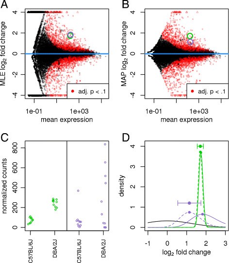
104 |
105 | The fanning out on the left indicates that the logFC often tend to be higher for very lowly expressed genes.
106 |
107 | The reasons are the same as for the underlying counts.
108 |
109 |
110 | ## Why does the heteroscedasticity matter?
111 |
112 | Because we're using models to gauge whether the difference in read counts is greater than expected by chance
113 | when comparing the values from group 1 (e.g. "WT") to the values from group 2 (e.g. "SNF2.KO").
114 |
115 | **Ordinary linear models** assume that the variance is constant and does not depend on the mean.
116 | That means, linear models will only work with **homoscedastic** data.
117 | Knowing what we just learnt about read count data properties, we can therefore rule out that simple linear models might be applied 'as is' -- not even with log-transformed data (as shown above)!
118 |
119 | This is why we turned to **generalized linear models** which allow us to use models where we can **include the mean-variance relationship**.
120 | GLM with negative binomial or Poisson regression do not make the assumption that the variance is equal for all values, instead they explicitly model the variance -- using a relationship that we have to choose.
121 | For Poisson, that relationship is `mean = variance`.
122 | For negative binomial models, we can choose even more complicated relationships, e.g. a quadratic relationship as it was chosen by [McCarthy et al.](https://academic.oup.com/nar/article/40/10/4288/2411520) for their `edgeR` package.
123 |
124 | That same paper also offers a nice discussion of the properties of the noise (coefficient of variation) with the main message being:
125 |
126 | 1. Total CV = biological noise + technical noise
127 | 2. technical noise will be greater for small count genes
128 |
129 | Here are the direct quotes from [McCarthy et al.](https://academic.oup.com/nar/article/40/10/4288/2411520) related to this:
130 |
131 | >The coefficient of variation (CV) of RNA-seq counts should be a decreasing function of count size for small to moderate counts but for larger counts should asymptote to a value that depends on biological variability
132 | >The first term arises from the technical variability associated with sequencing, and gradually decreases with expected count size, while biological variation remains roughly constant. For large counts, the CV is determined mainly by biological variation.
133 |
134 | >The technical CV decreases as the size of the counts increases. BCV on the other hand does not. BCV is therefore likely to be the dominant source of uncertainty for high-count genes, so reliable estimation of BCV is crucial for realistic assessment of differential expression in RNA-Seq experiments. If the abundance of each gene varies between replicate RNA samples in such a way that the genewise standard deviations are proportional to the genewise means, a commonly occurring property of measurements on physical quantities, then it is reasonable to suppose that BCV is approximately constant across genes.
135 |
136 |
137 | ## What does "overdispersion" mean and how is it related?
138 |
139 |
140 | Overdispersion refers to the observation that the variance tends to be *greater* than the mean expression.
141 | This again is an argument against the use of a simple Poisson model where the relationship between mean and variance would be fixed as `mean = variance`.
142 |
143 |
144 | ## Summary
145 |
146 | * Heteroskedasticity is simply the absence of equal variances across the entire spectrum of read count values.
147 | * Depending on whether the counts are log-transformed, the variance is higher for low-count genes (log) or high-count genes (untransformed).
148 |
--------------------------------------------------------------------------------
/RNA_heteroskedasticity.Rmd:
--------------------------------------------------------------------------------
1 | ---
2 | output:
3 | html_document:
4 | code_folding: hide
5 | theme: paper
6 | keep_md: true
7 | editor_options:
8 | chunk_output_type: console
9 | ---
10 |
11 | # Exploring heteroskedasticity
12 |
13 | ```{r setup, include=FALSE}
14 | knitr::opts_chunk$set(echo = TRUE, message=FALSE)
15 | ```
16 |
17 | ```{r include=FALSE}
18 | library(DESeq2)
19 | library(magrittr)
20 | library(data.table)
21 | library(ggplot2); theme_set(theme_bw(base_size = 12))
22 | library(patchwork)
23 | library(scales)
24 | # should have the DESeq object, DESeq.ds
25 | #load("~/Documents/Teaching/ANGSD/data/RNAseqGierlinski.RData")
26 | ```
27 |
28 | ```{r prep_object, warning=FALSE}
29 | ## read counts
30 | featCounts <- read.table("~/Documents/Teaching/ANGSD/data/featCounts_Gierlinski_genes.txt", header=TRUE, row.names = 1)
31 | names(featCounts) <- names(featCounts) %>% gsub(".*alignment\\.", "", .) %>% gsub("_Aligned.*", "",.)
32 | counts.mat <- as.matrix(featCounts[, -c(1:5)])
33 |
34 | ## sample info
35 | samples <- data.frame(condition = gsub("_.*", "", colnames(counts.mat)),
36 | row.names = colnames(counts.mat))
37 | samples$condition <- ifelse(samples$condition == "SNF2", "SNF2.KO", samples$condition)
38 |
39 | ## DESeq2 object
40 | dds <- DESeqDataSetFromMatrix(counts.mat, colData = samples, design = ~condition)
41 | # normalizing for diffs in sequencing depth and abundances per sample
42 | dds <- estimateSizeFactors(dds)
43 | ```
44 |
45 | **Heteroskedasticity** = absence of homoskedasticity.
46 | Where homoscedasticity is defined as ["the property of having equal statistical variances"](https://www.merriam-webster.com/dictionary/homoscedasticity).
47 |
48 | Historically, **log-transformation** was proposed to counteract heteroscedasticity.
49 | However, read counts retain unequal variabilities, even after log-transformation.
50 | As described by [Law et al.](https://genomebiology.biomedcentral.com/articles/10.1186/gb-2014-15-2-r29):
51 |
52 | > Large log-counts have much larger standard deviations than small counts.
53 | > A logarithmic transformation counteracts this, but it overdoes it. Now, large counts have smaller standard deviations than small log-counts.
54 |
55 | ```{r eval=FALSE}
56 | ## Greater variability across replicates for low-count genes
57 | counts(dds, normalized = TRUE) %>% .[,1:2] %>% log2 %>%
58 | plot(., main = "Greater variability of library-size-norm,\nlog-transformed counts for small count genes")
59 | ```
60 |
61 | ```{r fig.width = 8, warning=FALSE}
62 | ## meanSDPlot (vsn library)
63 | rowV = function(x, Mean) {
64 | sqr = function(x) x*x
65 | n = rowSums(!is.na(x))
66 | n[n<1] = NA
67 | return(rowSums(sqr(x-Mean))/(n-1))
68 | }
69 |
70 | mean.exprs = counts(dds[, dds$condition == "WT"], normalized = TRUE) %>% rowMeans(., na.rm = TRUE)
71 | vars.exprs = counts(dds[, dds$condition == "WT"], normalized = TRUE) %>%
72 | rowV(., Mean = mean.exprs)
73 | sd.exprs <- sqrt(vars.exprs)
74 | #vars <- sqrt(rowSums((x-means)^2)/(nlibs-1))
75 |
76 |
77 | ## log-transformed data
78 | mean.log2exprs = counts(dds[, dds$condition == "WT"], normalized = TRUE) %>% log2 %>%
79 | rowMeans(., na.rm = TRUE)
80 | vars.log2exprs = counts(dds[, dds$condition == "WT"], normalized = TRUE) %>% log2 %>%
81 | rowV(., Mean = mean.log2exprs)
82 | sd.log2exprs <- sqrt(vars.log2exprs)
83 | #vars <- sqrt(rowSums((x-means)^2)/(nlibs-1))
84 |
85 | par(mfrow=c(1,2))
86 | plot(log2(mean.exprs), log2(sd.exprs), main = "Sd depends on the mean", cex = .2, lwd = .1)
87 | plot(mean.log2exprs, sd.log2exprs, main = "Sd depends on the mean\nlog-transformed counts", cex = .2, lwd = .1)
88 |
89 | #vsn::meanSdPlot(log2(counts(dds[, dds$condition == "WT"], normalized =TRUE)))
90 | #plot(mean.exprs, vars.exprs, main = "Var depends on the mean", xlim = c(0,1000), ylim = c(0, 2000))
91 | #plot(mean.exprs, vars.exprs, main = "Var depends on the mean", xlim = c(0,20), ylim = c(0, 20))
92 | ```
93 |
94 | The greater the mean expression, the greater the variance.
95 | The greater the log-transformed expression, the smaller the variance as the average expression value and the actual expression value (`x`) are closer together.
96 |
97 |
98 | Click here for some toy examples to illustrate that point.
99 |
100 | ```{r }
101 | 1000 - 990
102 | log2(1000) - log2(990)
103 |
104 | 10 - 9
105 | log2(10) - log2(9)
106 | ```
107 |
108 |
109 |
110 | Intuitively, one can also see that the "spread" of the data points is greater for low-count values:
111 |
112 | ```{r}
113 | counts(dds, normalized = TRUE) %>% .[,c(1,2)] %>% log2 %>% plot
114 | ```
115 |
116 | ```{r eval=FALSE}
117 | # example with high expression
118 | mean.exprs %>% sort %>% tail # YKL060C
119 | # example with low expression
120 | mean.exprs[mean.exprs > 0] %>% sort %>% head #YPR099C
121 | ```
122 | ```{r}
123 | high.exprsd <- "YKL060C"
124 | low.exprsd <- "YPR099C"
125 | ```
126 |
127 | While the absolute values of SD/Var are higher for high-count genes,
128 | the **magnitude** of the noise is greater for the low-count genes:
129 |
130 | ```{r fig.width = 8}
131 | noise.mag <- sd.exprs[c(high.exprsd, low.exprsd)] / mean.exprs[c(high.exprsd, low.exprsd)]
132 |
133 | p1 <- counts(dds[high.exprsd,], normalized=TRUE) %>% t %>%
134 | as.data.table(., keep.rownames = "sample") %>%
135 | ggplot(., aes(x = gsub("_.*", "", sample), y = YKL060C)) +
136 | geom_point(size = 4, alpha = .5, shape = 1) +
137 | xlab("condition") +
138 | ggtitle("Highly expressed gene", subtitle = paste("SD:", sd.exprs[high.exprsd], "\nSD/mean:", noise.mag[high.exprsd]))
139 |
140 | p2 <- counts(dds[low.exprsd,], normalized=TRUE) %>% t %>%
141 | as.data.table(., keep.rownames = "sample") %>%
142 | ggplot(., aes(x = gsub("_.*", "", sample), y = YPR099C)) +
143 | geom_point(size = 4, alpha = .5, shape = 1) +
144 | xlab("condition") +
145 | ggtitle("Lowly expressed gene", subtitle = paste("SD:", sd.exprs[low.exprsd], "\nSD/mean:", noise.mag[low.exprsd]))
146 |
147 | p1 + p2 + plot_annotation(title = "Lib-size norm. counts")
148 | ```
149 | ```{r fig.width = 8}
150 | noiselog2.mag <- sd.log2exprs[c(high.exprsd, low.exprsd)] / mean.log2exprs[c(high.exprsd, low.exprsd)]
151 |
152 | p1 <- log2(counts(dds[high.exprsd,], normalized=TRUE)) %>% t %>%
153 | as.data.table(., keep.rownames = "sample") %>%
154 | ggplot(., aes(x = gsub("_.*", "", sample), y = YKL060C)) +
155 | geom_point(size = 4, alpha = .5, shape = 1) +
156 | xlab("condition") +
157 | ggtitle("Highly expressed gene", subtitle = paste("SD:", sd.log2exprs[high.exprsd], "\nSD/mean:", noiselog2.mag[high.exprsd]))
158 |
159 | p2 <- log2(counts(dds[low.exprsd,], normalized=TRUE)) %>% t %>%
160 | as.data.table(., keep.rownames = "sample") %>%
161 | ggplot(., aes(x = gsub("_.*", "", sample), y = YPR099C)) +
162 | geom_point(size = 4, alpha = .5, shape = 1) +
163 | xlab("condition") +
164 | ggtitle("Lowly expressed gene", subtitle = paste("SD:", sd.log2exprs[low.exprsd], "\nSD/mean:", noiselog2.mag[low.exprsd]))
165 |
166 | p1 + p2 + plot_annotation(title = "Lib-size norm., log2-transformed counts")
167 | ```
168 |
169 | This is true irrespective of log-transformation:
170 |
171 | ```{r fig.width = 12}
172 | cvs <- sd.exprs/mean.exprs
173 | cvs.log2 <- sd.log2exprs / mean.log2exprs
174 |
175 | #par(mfrow = c(1,2))
176 | #plot(log2(mean.exprs), log2(cvs), main = "Coefficient of variation of counts")
177 | #plot(mean.log2exprs, cvs.log2, main = "Coefficient of variation of log-transformed counts")
178 | p1 <- ggplot(data.frame(meanExprs = mean.exprs, noise.mag = cvs),
179 | aes(x = mean.exprs, y = noise.mag)) + geom_point() +
180 | scale_y_continuous(trans = log2_trans()) +
181 | scale_x_continuous(trans=log2_trans()) +
182 | ggtitle("Coefficient of variation of counts")
183 | p2 <- ggplot(data.frame(mean.log2Exprs = mean.log2exprs, noise.mag_of_log2ExprsValues = cvs.log2),
184 | aes(x = mean.exprs, y = noise.mag_of_log2ExprsValues)) + geom_point() +
185 | scale_y_continuous(trans = log2_trans()) +
186 | scale_x_continuous(trans=log2_trans()) +
187 | ggtitle("Coefficient of variation of log-transformed counts")
188 | p1 | p2
189 | ```
190 |
191 |
192 | The value that I named "magnitude of noise" (`noise.mag` in the code) happens to match the definition of the [**coefficient of variation**](https://en.wikipedia.org/wiki/Coefficient_of_variation)
193 |
194 | ### Fold changes are also heteroskedastic
195 |
196 | [Love & Huber](https://genomebiology.biomedcentral.com/articles/10.1186/s13059-014-0550-8) demonstrated heteroskedasticity as "variance of log-fold changes depending on mean count".
197 |
198 | >weakly expressed genes seem to show much stronger **differences** between the compared mouse strains than strongly expressed genes. This phenomenon, seen in most HTS datasets, is a direct consequence of dealing with count data, in which **ratios are inherently noisier when counts are low**
199 |
200 | 
201 |
202 | The fanning out on the left indicates that the logFC often tend to be higher for very lowly expressed genes.
203 |
204 | The reasons are the same as for the underlying counts.
205 |
206 |
207 | ## Why does the heteroscedasticity matter?
208 |
209 | Because we're using models to gauge whether the difference in read counts is greater than expected by chance
210 | when comparing the values from group 1 (e.g. "WT") to the values from group 2 (e.g. "SNF2.KO").
211 |
212 | **Ordinary linear models** assume that the variance is constant and does not depend on the mean.
213 | That means, linear models will only work with **homoscedastic** data.
214 | Knowing what we just learnt about read count data properties, we can therefore rule out that simple linear models might be applied 'as is' -- not even with log-transformed data (as shown above)!
215 |
216 | This is why we turned to **generalized linear models** which allow us to use models where we can **include the mean-variance relationship**.
217 | GLM with negative binomial or Poisson regression do not make the assumption that the variance is equal for all values, instead they explicitly model the variance -- using a relationship that we have to choose.
218 | For Poisson, that relationship is `mean = variance`.
219 | For negative binomial models, we can choose even more complicated relationships, e.g. a quadratic relationship as it was chosen by [McCarthy et al.](https://academic.oup.com/nar/article/40/10/4288/2411520) for their `edgeR` package.
220 |
221 | That same paper also offers a nice discussion of the properties of the noise (coefficient of variation) with the main message being:
222 |
223 | 1. Total CV = biological noise + technical noise
224 | 2. technical noise will be greater for small count genes
225 |
226 | Here are the direct quotes from [McCarthy et al.](https://academic.oup.com/nar/article/40/10/4288/2411520) related to this:
227 |
228 | >The coefficient of variation (CV) of RNA-seq counts should be a decreasing function of count size for small to moderate counts but for larger counts should asymptote to a value that depends on biological variability
229 | >The first term arises from the technical variability associated with sequencing, and gradually decreases with expected count size, while biological variation remains roughly constant. For large counts, the CV is determined mainly by biological variation.
230 |
231 | >The technical CV decreases as the size of the counts increases. BCV on the other hand does not. BCV is therefore likely to be the dominant source of uncertainty for high-count genes, so reliable estimation of BCV is crucial for realistic assessment of differential expression in RNA-Seq experiments. If the abundance of each gene varies between replicate RNA samples in such a way that the genewise standard deviations are proportional to the genewise means, a commonly occurring property of measurements on physical quantities, then it is reasonable to suppose that BCV is approximately constant across genes.
232 |
233 | ## What does "overdispersion" mean and how is it related?
234 |
235 | Overdispersion refers to the observation that the variance tends to be *greater* than the mean expression.
236 | This again is an argument against the use of a simple Poisson model where the relationship between mean and variance would be fixed as `mean = variance`.
237 |
238 | ## Summary
239 |
240 | * Heteroskedasticity is simply the absence of equal variances across the entire spectrum of read count values.
241 | * Depending on whether the counts are log-transformed, the variance is higher for low-count genes (log) or high-count genes (untransformed).
242 |
--------------------------------------------------------------------------------
/CITE-seq.md:
--------------------------------------------------------------------------------
1 | CITE-seq
2 | ===========
3 |
4 | Cellular indexing of transcriptomes and epitopes by sequencing (CITE-seq) is a
5 | technique that quantifies both gene expression and the abundance of selected
6 | surface proteins in each cell simultaneously ([Stoeckius et al. 2017](https://www.nature.com/articles/nmeth.4380)).
7 |
8 | In this approach, cells are first labelled with **antibodies that have been
9 | conjugated to synthetic RNA tags**.
10 | A cell with a higher abundance of a target protein will be bound by more antibodies,
11 | causing more molecules of the corresponding antibody-derived tag (ADT) to be attached to that cell. [Ref.OSCA](http://bioconductor.org/books/release/OSCA/integrating-with-protein-abundance.html)
12 |
13 | 
14 |
15 | 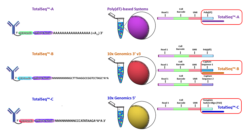
16 |
17 | **Cell Hashing** is based on the exact same principle except that one aims to find a target that's ubiquitously expressed across all cells within the samples. [Stoeckius et al., 2018](https://genomebiology.biomedcentral.com/articles/10.1186/s13059-018-1603-1)
18 |
19 | BioLegend supports the protocols with [TotalSeq Reagents](https://www.biolegend.com/en-us/totalseq), i.e. customized antibodies suitable for 10X Genomics' sequencing prep.
20 | For the differences between TotalSeq A, B, C see [10X Genomics reply](https://kb.10xgenomics.com/hc/en-us/articles/360019665352-What-is-the-difference-between-TotalSeq-A-B-and-C-) -- in short, their differences have to do with the different sequencing chemistries of different 10X Genomics' protocols.
21 |
22 | --------------
23 |
24 | * [How CellRanger handles CITE-seq data](#cellranger)
25 | * [How to code with CITE-seq data](#code) (mostly excerpts from [OSCA](http://bioconductor.org/books/release/OSCA/integrating-with-protein-abundance.html))
26 | * [Reading in](#start)
27 | * [QC](#qc)
28 | * [Normalization](#normalizing)
29 | * [Clustering](#clustering)
30 | * [Integration with expression data](#combi)
31 | * [Hash tags](#hto)
32 |
33 | --------------
34 |
35 |
36 | ## CellRanger considerations
37 |
38 | * `CellRanger` doesn't explicitly support CITE-seq, but they support generic "antibody capture" results
39 | - e.g. dextramers, antigens
40 | * The entries in their `metrics_summary.csv` are explained [here](https://support.10xgenomics.com/single-cell-gene-expression/software/pipelines/latest/output/antibody-metrics)
41 | - e.g. `Antibody: Fraction Antibody Reads in Aggregate Barcodes`: Fraction of reads lost after removing aggregate barcodes.
42 | * One specific issue with antibodies are **protein aggregates** that cause a few GEMs to have extremely high UMI counts.
43 | - "Currently, we consider a barcode an aggregate if it has more than 10K reads, 50% of which were corrected [`$`](#correction)" [Ref](https://support.10xgenomics.com/single-cell-gene-expression/software/pipelines/latest/algorithms/antibody)
44 | - in addition, "Cell Ranger directly uses protein counts to deduce aggregation events.", i.e. "seeing high counts of many unrelated proteins in a GEM is a sign that such a GEM contains protein aggregates" [Ref](https://support.10xgenomics.com/single-cell-gene-expression/software/pipelines/latest/algorithms/antibody) - if >5 antibodies with min. 1000 counts are detected, GEMs that are in the 25 highest counts across all GEMs will be flagged if the required number of antibodies exceed a pre-deinfed threshold
45 | - a high correction rate is therefore used to flag for protein aggregation
46 | - barcodes with evidence of protein aggregation are removed from the final feature-barcode matrix
47 | * "Antibody aggregation could be triggered by partial unfolding of its domains, leading to monomer-monomer association followed by nucleation and growth. Although the aggregation propensities of antibodies and antibody-based proteins can be affected by the external experimental conditions, they are strongly dependent on the intrinsic antibody properties as determined by their sequences and structures" [Li et al., 2016](https://www.mdpi.com/2073-4468/5/3/19)
48 |
49 |
50 | `$`*CellRanger's UMI correction*: Before counting UMIs, Cell Ranger attempts to **correct for sequencing errors** in the UMI sequences. Reads that were confidently mapped to the transcriptome are placed into groups that share the same barcode, UMI, and gene annotation. If two groups of reads have the same barcode and gene, but their UMIs differ by a single base (i.e., are Hamming distance 1 apart), then one of the UMIs was likely introduced by a substitution error in sequencing. In this case, the UMI of the less-supported read group is corrected to the UMI with higher support. [Ref](https://support.10xgenomics.com/single-cell-gene-expression/software/pipelines/latest/algorithms/overview)
51 |
52 |
53 |
54 | **[How should the ADT data be incorporated into the analysis?](http://bioconductor.org/books/release/OSCA/integrating-with-protein-abundance.html#quality-control-1)**
55 |
56 | # Technical info from 10X
57 |
58 | * how 10X measures the antibody levels
59 | - [Algorithm details](https://support.10xgenomics.com/single-cell-gene-expression/software/pipelines/latest/algorithms/antibody)
60 | - [Antibody metrics](https://support.10xgenomics.com/single-cell-gene-expression/software/pipelines/latest/output/antibody-metrics)
61 |
62 | * TotalSeq-C is a line of antibody-oligonucleotide conjugates supplied by BioLegend that are compatible with the Single Cell 5' assay. The Feature Barcode sequence appears at a fixed position (base 10) in the R2 read.
63 |
64 | # How should the ADT data be incorporated into the analysis?
65 |
66 | While we have counts for both ADTs and transcripts, there are fundamental differences
67 | in nature of the data that make it difficult to treat the former as additional features
68 | in the latter:
69 |
70 | * small number of antibodies vs. entire transcriptome
71 | * coverage of the ADTs is much deeper (sequencing resources are concentrated into a smaller number of features)
72 | * use of antibodies against protein targets involves consideration of separate biases compared to those observed for transcripts.
73 |
74 | from [OSCA](http://bioconductor.org/books/release/OSCA/integrating-with-protein-abundance.html)
75 |
76 |
77 | ## Reading in the data
78 |
79 | from [OSCA](http://bioconductor.org/books/release/OSCA/integrating-with-protein-abundance.html)
80 |
81 |
82 | ```
83 | # CellRanger data here:
84 | /athena/abc/scratch/paz2005/projects/2020_11_sofia_scrna/cellranger_v5_out
85 | ```
86 |
87 | ```
88 | conda create --name citeseq
89 | conda install -c conda-forge r-base
90 | conda install -c conda-forge r-data.table
91 | conda install -c bioconda bioconductor-scuttle
92 | conda install -c bioconda bioconductor-singlecellexperiment
93 | conda install -c r r-ggplot2
94 | ```
95 |
96 | * `SingleCellExperiment` class --> "alternative Experiment"
97 | - to store data for different sets of features but the same cells
98 | - can be used to store another SE object inside the SCE object
99 | - often used for spike-in data
100 | - isolates the two sets of features to ensure that analyses on one set o not use data from the other set
101 |
102 | ```{r}
103 | sce <- splitAltExps(sce, rowData(sce)$Type)
104 | altExpNames(sce) # Can be used like any other SingleCellExperiment.
105 |
106 | # ADT counts are usually not sparse so storage as a sparse matrix provides no advantage
107 | counts(altExp(sce)) <- as.matrix(counts(altExp(sce)))
108 | counts(altExp(sce))[,1:10] # sneak peek
109 | ```
110 |
111 |
112 | ## QC
113 |
114 | ### Genes: low mito content!
115 |
116 | ```{r}
117 | mito <- grep("^MT-", rowData(sce)$Symbol)
118 | df <- perCellQCMetrics(sce, subsets=list(Mito=mito))
119 | mito.discard <- isOutlier(df$subsets_Mito_percent, type="higher")
120 | ```
121 |
122 |
123 | ### ADTs
124 |
125 | * remove cells that have failed to capture and/or sequence the ADTs
126 | * background contamination: free antibody or antibody bound to cell fragments
127 |
128 | ALL ADTs SHOULD HAVE READS! [otherwise something went wront with the processing!]
129 |
130 | ```{r}
131 | # remove cells that have unusually low numbers of detected ADTs
132 | # Applied on the alternative experiment containing the ADT counts:
133 | library(scuttle)
134 | df.ab <- perCellQCMetrics(altExp(sce))
135 |
136 | n.nonzero <- sum(!rowAlls(counts(altExp(sce)), value=0L)) # less than or equal to half of the total number of tags
137 | ab.discard <- df.ab$detected <= n.nonzero/2 #
138 | summary(ab.discard)
139 | ```
140 |
141 | ### Final filtering step
142 |
143 | ```{r}
144 | discard <- ab.discard | mito.discard
145 | sce <- sce[,!discard]
146 | ```
147 |
148 |
149 | ## Normalizing ADTs
150 |
151 | >simplest approach is to normalize on the total ADT counts
152 | >However, ideally, we would like to compute size factors that adjust for the composition biases. This usually requires an assumption that most ADTs are not differentially expressed between cell types/states.
153 |
154 | >We consider the baseline ADT profile to be a combination of weak constitutive expression and ambient contamination, both of which should be constant across the population. We estimate this profile by assuming that the distribution of abundances for each ADT should be bimodal, where one population of cells exhibits low baseline expression and another population upregulates the corresponding protein target. We then use all cells in the lower mode to compute the baseline abundance for that ADT. This entire calculation is performed by the inferAmbience() function
155 | > We use a DESeq2-like approach to compute size factors against the baseline profile. Specifically, the size factor for each cell is defined as the median of the ratios of that cell’s counts to the baseline profile. If the abundances for most ADTs in each cell are baseline-derived, they should be roughly constant across cells; any systematic differences in the ratios correspond to cell-specific biases in sequencing coverage and are captured by the size factor. The use of the median protects against the minority of ADTs corresponding to genuinely expressed targets.
156 |
157 | ```{r}
158 | baseline <- inferAmbience(counts(altExp(sce)))
159 | # Distribution of (log-)counts for each ADT in the PBMC dataset, with the inferred ambient abundance marked by the black dot.
160 | plotExpression(altExp(sce), features=rownames(altExp(sce)), exprs_values="counts") +
161 | scale_y_log10() +
162 | geom_point(data=data.frame(x=names(baseline), y=baseline), mapping=aes(x=x, y=y), cex=3)
163 |
164 | sf.amb <- medianSizeFactors(altExp(sce), reference=baseline)
165 | # add median-based size factors to the altExp
166 | sizeFactors(altExp(sce)) <- sf.amb
167 |
168 | # logNorm will transform both expression and ADT
169 | sce <- logNormCounts(sce, use.altexps=TRUE)
170 | ```
171 |
172 |
173 | ## Clustering
174 |
175 | >Unlike transcript-based counts, feature selection is largely unnecessary for analyzing ADT data. This is because feature selection has already occurred during experimental design where the manual choice of target proteins means that all ADTs correspond to interesting features by definition
176 | > ADT abundances are cleaner (larger counts, stronger signal) for more robust identification of broad cell types
177 |
178 | ```{r}
179 | # Set d=NA so that the function does not perform PCA.
180 | g.adt <- buildSNNGraph(altExp(sce), d=NA)
181 | clusters.adt <- igraph::cluster_walktrap(g.adt)$membership
182 |
183 | # Generating a t-SNE plot.
184 | library(scater)
185 | set.seed(1010010)
186 | altExp(sce) <- runTSNE(altExp(sce))
187 | colLabels(altExp(sce)) <- factor(clusters.adt)
188 | plotTSNE(altExp(sce), colour_by="label", text_by="label", text_col="red")
189 | ```
190 |
191 |
192 | ## Integration with gene expression data
193 |
194 | > If the aim is to test for differences in the functional readout (e.g. using antibodies to target the influenza peptide-MHCII complexes), a natural analysis strategy is to *use the transcript data for clustering* (Figure 20.13) and perform differential testing between clusters or conditions for the relevant ADTs. The main appeal of this approach is that it avoids data snooping (Section 11.5.1) as the clusters are defined without knowledge of the ADTs. This improves the statistical rigor of the subsequent differential testing on the ADT abundances
195 |
196 | More ideas:
197 |
198 |
199 | ## Hash tagging
200 |
201 | From [Stoeckius et al., 2018](https://genomebiology.biomedcentral.com/articles/10.1186/s13059-018-1603-1#Sec18):
202 |
203 | >HTO raw counts were normalized using centered log ratio (CLR) transformation, where counts were divided by the geometric mean of an HTO across cells and log-transformed
204 | >
205 |
206 | Seurat's `HTODemux()` function
207 |
208 | * k-medoid clustering on normalized HTO values --> cells are separated into *K* clusters
209 | * "negative" distribution: cluster with lowest average value = negative group for that HTO
210 | * .99 quantile of NB fit used as a threshold to classify cells as positive or negative
211 | * cells with more than one positive HTO call: doublets
212 |
213 | [OSCA recommends `DropletUtils`](http://bioconductor.org/books/release/OSCA/droplet-processing.html#demultiplexing-on-hto-abundance): `hashedDrops()`
214 |
215 | > assuming that each HTO has a bimodal distribution where the lower peak corresponds to ambient contamination in cells that do not belong to that HTO’s sample. Counts are then averaged across all cells in the lower mode to obtain the relative abundance of that HTO
216 |
217 |
218 |
--------------------------------------------------------------------------------
/notes_10Q.md:
--------------------------------------------------------------------------------
1 | [Williams2017](@doi:10.1111/nyas.13207):
2 |
3 | "it is self‐evident that life science is data science. High‐throughput nucleic acid sequencing has given rise to massive amounts of data, including repositories such as the NCBI Sequence Read Archive (SRA). The SRA's 4.5 quadrillion bases of sequence are certain to be an invaluable resource for discovery. Clearly, data production is no longer a bottleneck; genome sequencing costs have decreased 1000‐fold in the last decade and are undergoing another steep decrease this year.2 Advances in image acquisition and analysis promise to accelerate on par with high‐throughput sequencing"
4 |
5 | [Rossi2018](@doi:10.3389/fdigh.2018.00013)
6 |
7 | * "Medicine is supported by observations and data and for certain aspects medicine is becoming a data science supported by clinicians. "
8 | * "More data and the ability to efficiently handle them is a significant advantage not only for clinicians and life science researchers, but for drugs producers too."
9 | "Big data domains are those able to store data in the order of magnitude of Peta to Exabyte. One Exabyte equals 1 billion Gigabytes, being the Gigabyte the scale in which the current portable storage cards are measured (our smartphones work with memories of 16 Gigabytes on average). Storage volumes are actually much smaller than volumes produced by the acquisition processes, which globally sum up to the order of zettabytes (the actual footprint), due to the fact that intermediate data are often heavily pruned and selected by quality control and data reduction processes. According to the recorded historical growth rate, the growth of DNA sequencing (in number of genomes) is almost twice as fast as predicted by Moore's Law, i.e., it doubled every 7 months since the first Illumina genome sequences in 2008.
10 | Due to these numbers **genomics is comparable to other big data domains, such as astronomy, physics, and social media** (particularly Twitter and YouTube). Research institutions and consortia are sequencing genomes at unprecedented rhythms, collecting genomic data for thousands of individuals, such as the Genomics England project (Genomics England, 2017) or Saudi Human Genome Program (Saudi Genome Project Team, 2015)."
11 | * "Most laboratory equipment produces bigger volumes of data than it did in the past, and data points available in a common lab pile up to quantities not amenable to traditional processing such as electronic spreadsheets. "
12 | * "As a consequence, the many flavors of bioinformatics and computational biology skills are now a must-have in the technologically advanced research laboratories or R&D departments: companies and research institutions, as well as single laboratories, should also promote and organize computationally skilled personnel"
13 |
14 | [Bartlett2017](@doi:10.1186/s12859-017-1730-9)
15 |
16 | * "Bioinformatics has multitudinous identities, organisational alignments and disciplinary links. This variety allows bioinformaticians and bioinformatic work to contribute to much (if not most) of life science research in profound ways."
17 | * "The power of bioinformatic work is shaped by its dependency on life science work, which combined with the black-boxed character of bioinformatic expertise further contributes to situating bioinformatics on the periphery of the life sciences. "
18 | * " show that bioinformatic work is operating in a social, institutional, and cultural context that presents obstacles to it receiving due credit despite its increasing importance."
19 | * "Science itself is about producing knowledge, but the day-to-day work of science is also about securing resources, crafting collaborations, earning credit, building reputations, as well as negotiating what it is that counts as ‘important’, ‘relevant’, ‘significant’, or even ‘interesting’. "
20 | * "Alongside their methodologies, skills and expertise, biologists and computer scientists have also brought their respective research cultures – their values and priorities – into bioinformatics, creating a hybrid inter-discipline and a hybrid culture [3]. This means that not only are there cultural as well as intellectual boundaries between biologists, computer scientists, and bioinformaticians, but there are also points of friction and tension within the broad, heterogeneous field of bioinformatics itself "
21 | * "It is not surprising, then, that those we have spoken to have reported that many view bioinformatics as a ‘service’, rather than as a scientific field in its own right. In some cases, the development of tools that are used by life scientists renders the intellectual contribution of bioinformaticians invisible, hidden in the ‘black box’"
22 | * **interdisciplinary work is risky** It falls outside of established power structures, it does not fit evaluation models built for disciplinary scientific work [8] and, related to these facts, it is does not generate the same degree of respect from both peers and public, partly because the lack of a decades-long track record of accomplishments.
23 | * we increasingly see bioinformaticians co-designing laboratory experiments and entire studies to optimise inputs, and by consequence, optimise outputs. Bioinformaticians are, without physically producing primary inscriptions, increasingly taking responsibility for them. But despite that responsibility growing, translation of these contributions into scientific credit lags well behind.
24 |
25 | [Bartlett2018](@doi:10.1177/2053951718768831):
26 |
27 | * middling: bridging the gap between computer science and biology but as yet not forming its own, coherent, disciplinary space, nor occupying those of its ‘parental’ disciplines
28 | * Importantly, biologists have institutional ‘ownership’ of the data of Big Data biology.
29 | * The locus of legitimate interpretation for Big Data biology is located firmly within the epistemic, disciplinary culture of biology: data are produced within the discipline, in laboratories, by biologists, or by computer scientists with biological sensibilities in mind. That is, although computational and statistical expertise has been drawn into the discipline, bringing with it a new style of statistical reasoning (Leonelli, 2012; Lewis et al., 2016), it has been done so in a way that positions it subordinate to the disciplinary concerns of biology
30 | * Expertise in data analysis alone is not deemed sufficient to make legitimate biological knowledge claims. Biologists, as the creators of the primary inscriptions and the holders of cultural and institutional power, are the legitimate interpreters of Big Data biology, with the computer scientists/bioinformaticians who produce the ‘secondary inscriptions’ being dependent on, and deferring to, biologists. Bioinformatics may be an offshoot of biology, but it is tied inextricably to the disciplinary culture and institutions of biology. Physics, with a long tradition of dealing with Big Data, ‘produces’ its own computer scientists, and ‘Big Data’ physics is, mostly, conducted within the disciplinary space of ‘physics’.
31 |
32 | [Lewis2016](@doi:10.1007/s11024-016-9304-y)
33 |
34 | * "Bioinformatics – the so-called shotgun marriage between biology and computer science – is an interdiscipline. Despite interdisciplinarity being seen as a virtue, for having the capacity to solve complex problems and foster innovation, it has the potential to place projects and people in anomalous categories"
35 |
36 | [Chasapi2019](@doi:10.1371/journal.pcbi.1007532)
37 | The utter relevance to biomedical research and human health started emerging as a serious proposition, following the sequencing of the human genome [31].
38 |
39 | [Wang2020](@doi:10.1080/14636778.2020.1843148)
40 | * "Bartlett, Lewis, and Williams (2016), examining struggles for epistemic authority over the emerging field of bioinformatics, suggest that biologists have retained cultural power as legitimate interpreters of biological world. Conversely the important contributions of diverse computational specialists in creating protocols, developing algorithms and data curation in processing data from large scale biological experiments– might not be recognised and thus rewarded/ valorised for example when the work was published in a biological science journal."
41 | * "Large scale bioinformatics centres are strategic sites where these new expert roles are being developed and elaborated."
42 | * * "Though commercial gene sequencing facilities had achieved high levels of efficiency in sequencing, questions have been raised about the quality and scientific value of outputs of large-scale and in particular commercial laboratories."
43 | * QUote from a BGI member: " it is highly possible that they are not able to achieve the goals if they do all jobs by themselves – the data, information and results could be out of their reach. Under such circumstances, computer scientists, mathematicians and others are needed to collect and process the data and information that the biologists want. I accept that the biologists are the predominant members in the research project team and researchers from other related disciplines are more supporting than deciding"
44 |
45 | [Vermeulen2016](@doi:10.1007/s00048-016-0141-8)
46 | The origin of big physics was traced back to the inter-war period when universities in California began collaborating to find a solution for the problems of power production and distribution (Galison 1992; Seidel 1992). Large-scale physics research spread internationally after the important contribution of large-scale physics research to World War II.
47 |
48 |
49 | [Tractenberg2019](@doi:10.1371/journal.pone.0225256)
50 | * "Bioinformatics, the discipline that evolved to harness computational approaches to manage and analyze life-science data, is inherently multi-disciplinary, and those trained in it therefore need to achieve an integrated understanding of both factual and procedural aspects of its diverse component fields."
51 | * Late/advanced Journeyman (J2) (e.g., doctorate holder), Bloom’s 5, late 6: expertly evaluate (review) and synthesize novel life-science knowledge, and integrate bioinformatics into research practice. The J2 Journeyman is independent and expert in a specific life-science area, and can select, apply and develop new methods. The J2 Journeyman formulates problems, considers the relevance of “what works” within this area to other life-science domains, so as to be an adaptable and creative scientific innovator without having to reinvent every wheel.
52 | * prioritizes the development of independent scientific reasoning and practice; it can therefore contribute to the cultivation of a next generation of bioinformaticians who are able to design rigorous, reproducible research, and critically analyze their and others’ work.
53 |
54 | [Feenstra2018](@doi:10.1093/bioinformatics/bty233)
55 |
56 | * "ability to translate research problems from one discipline to another, and communication with peers from different scientific backgrounds are key components. "
57 | * Chang (2015) analysed a year and a half of projects in their bioinformatics core facility, and found that 46 data analysis projects had required over 34 different types of analysis methods. The vast majority of projects thus required unique, one-off approaches that were tailor-made for the task at hand, had not been used before, and likely would not be used again. In other words, there is no routine, and each analysis project becomes a research project in itself, requiring staff at PhD level to perform effectively. Note, that the lack of generalizability of such methods may be another hurdle to publication for these researchers. It should be emphasized that translation, here between project requirement and method capability, seems to have been a key element of success.
58 | * We therefore expect that computational biologists, computer scientists and biologists—while learning and appreciating more about each other’s fields, and integrating more of each other’s approaches, methods and techniques into their own work—may likely continue their current course of intensive collaborations for some time to come
59 | * challenging research disciplines, which require practitioners to have a well-developed concept of the art of doing science, a high ability for mathematical and algorithmic abstraction, a broadly developed knowledge (balance), an ability to quickly absorb and integrate novel concepts (translate) and well-developed modelling, engineering and practical skills (focus). These aspects are all emphasized as critically important for the job market in the life sciences (Greene et al., 2016; Via et al., 2013; Welch et al., 2014), the data sciences (Dunn and Bourne, 2017; Lyon and Mattern, 2017; Pournaras, 2017; Seidl et al., 2018) and both (Brazas et al., 2017a; Greene et al., 2016).
60 |
61 | [Smith2015](@doi:10.3389/fgene.2015.00258)
62 | * Vincent and Charette (2015) make some excellent and compelling points in their article, and although I disagree with some of them, one of their final points resonated with me: “A good definition of a bioinformatician should not be based on a single concept …real bioinformaticians share a number of common characteristics …none of which [are] essential.” Perhaps a common characteristics that we share as bioinformaticians (and maybe this one should be essential) is a passion for using computers to understand the bewildering biological world that surrounds and encompasses us.
63 |
64 | [Smith2018](@doi:10.15252/embr.201846262)
65 | " At its surface, bioinformatics is a relevant, relatable, and stimulating discipline. At its heart, however, it is a dry, dense, and challenging topic to teach. If I describe the capabilities of user‐friendly software like Geneious, the students are interested and engaged. “This is awesome, Professor Smith! I didn't realize that I could explore all of these cool genomes right from my laptop without leaving the couch and with only rudimentary computer skills.” Bring up the finer points of the De Bruijn graph assembly method or Bayesian phylogenetics and half the class is heading for the door; and even some good old bioinformatics humor—“I hope everyone is having a BLASTX”—would not bring them back."
--------------------------------------------------------------------------------
/IntroToNGS_WCMGS.md:
--------------------------------------------------------------------------------
1 | In the last decade, extraordinary advances in high-throughput DNA sequencing have laid the foundation for addressing molecular questions at a genome-wide scale. Instead of investigating one locus at a time, researchers can now acquire data covering the entire genome in one single experiment.
2 | While these data sets can assist the elucidation of complex biological systems and diseases, they also require sophisticated solutions for data storage, processing, analysis and interpretation. Simply put: you won't get very far with Excel spreadsheets if you're looking at 30,000 genes at a time - in fact, to arrive at biologically meaningful values for 30,000 genes to begin looking at alreday takes a lot of data wrangling and processing!
3 |
4 | At WCM, several Core Facilities exist to enable researchers to take full advantage of the cutting-edge research possibilities related to high-throughput DNA sequencing experiments, ranging from optimized protocols for the different types of sequencing-related assays to high-performance computing environments and bioinformatics support.
5 | We strongly encourage you to tap into their expertise to help you set up your own experiments.
6 |
7 | The following paragraphs are very brief summaries of the most important points to consider when thinking about using high-throughput DNA sequencing experiments in your own work. They are by no means exhaustive, but they should give you an idea of the possibilities and as well as pitfalls of these types of experiments.
8 |
9 | * [Overview](#overview)
10 | * [WCM's infrastructure](#infrastructure)
11 | * [Parameters to consider for planning the experiment](#params)
12 | - [How many and what type of replicates?](#reps)
13 | - [Experimental design](#design)
14 | * [More resources](#resources)
15 | - [Meetings](#meetings)
16 | - [Classes at WCM](#courses)
17 | - [Self-paced reading and studying](#refs)
18 |
19 |
20 | ## Overview
21 |
22 | DNA sequencing is used for far more than actually reading the DNA sequence. The advent of massive parallel DNA sequencing (synonyms: shotgun sequencing, next-generation sequencing, deep sequencing) has enabled researchers to do quantitative counting of RNA and DNA molecules, which can be combined with more spophisticated biochemical set-ups allowing the interrogation of active transcription (RNA-seq, PRO-seq, GRO-seq) as well as egpigenetic DNA modifications (bisulfite sequencing), insights about protein-DNA interactions and histone mark distributions (ChIP-seq), the 3D structure of chromatin (ChIA-PET, ChIP-seq), and many more.
23 | Even antibody-stainings typically used for FACS analyses can now be translated into DNA reads (CITE-seq).
24 |
25 | The following figure taken from [Frese et al., 2013](http://www.mdpi.com/2079-7737/2/1/378) highlights some of the most commonly applied seq-based applications:
26 |
27 | 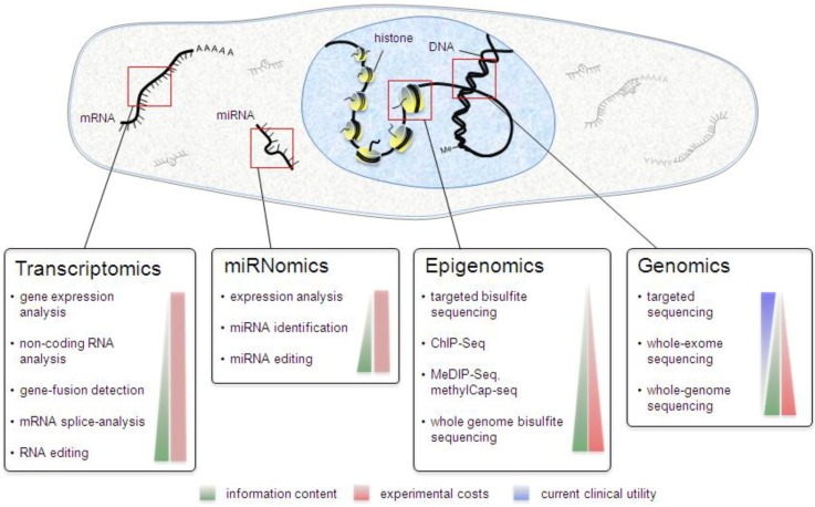
28 |
29 | For more details about the different high-throughput sequencing platforms and applications, see [Goodwin et al., 2016](http://dx.doi.org/10.1038/nrg.2016.49) and [Reuter et al., 2015](https://www.sciencedirect.com/science/article/pii/S1097276515003408).
30 |
31 | The general workflow of any experiment based on high-throughput DNA sequencing involves the following steps, whose optimal execution requires molecular biology as well as computational expertise.
32 |
33 | 1. **Sample prepration** This step is usually done by the molecular biologist.
34 | What type of starting material is needed depends on the type of assay. For RNA-seq, this would include RNA extraction from all samples of interest; for eRRBS, WGBS, exome-sequencing etc. DNA will have to be extracted; for ChIP-seq, chromatin will be purified, immunoprecipitated and eventually fragmented into small DNA pieces; and so on.
35 | 2. **Sequencing**
36 | 1. *Library preparation*: the RNA or DNA fragments delivered to the sequencing facility are (highly) amplified, and ligated to the adapters and primers that are needed for sequencing
37 | 2. *Sequencing-by-synthesis*: the libraries are loaded onto the lanes of a flow cell, in which the base pair order of every DNA fragment is determined using distinct fluorescent dyes for every nucleotide (for more details, see Section 1.3 of the [Introduction to RNA-seq](http://chagall.med.cornell.edu/RNASEQcourse/Intro2RNAseq.pdf) )
38 | 3. **Bioinformatics**
39 | 1. Quality control and *processing* of the raw sequencing reads, e.g., trimming of excess adapter sequences
40 | 2. Read *alignment* and QC
41 | 3. Additional *processing*, e.g. normalization to account for differences in sequencing depth (= total numbers of reads) per sample
42 | 4. Downstream analyses, e.g. identification of differentially expressed genes (RNA-seq), peaks (ChIP-seq), differentially methylated regions (eRRBS, WGBS), sequence variants (exome-seq), and so on
43 |
44 |
45 | ## WCM's infrastructure for high-throughput DNA sequencing experiments
46 |
47 | WCM offers assistance for virtually every step that's needed for the successful implementation and interpretation of experiments involving high-throughput DNA sequencing.
48 |
49 | * **Sequencing** and basic data processing: Genomics Core, [Epigenomics Core](http://epicore.med.cornell.edu/)
50 | * **Analysis**: [Applied Bioinformatics Core](abc.med.cornell.edu)
51 | * **Storage and high-performance computing servers**: Scientific Computing Unit
52 |
53 | 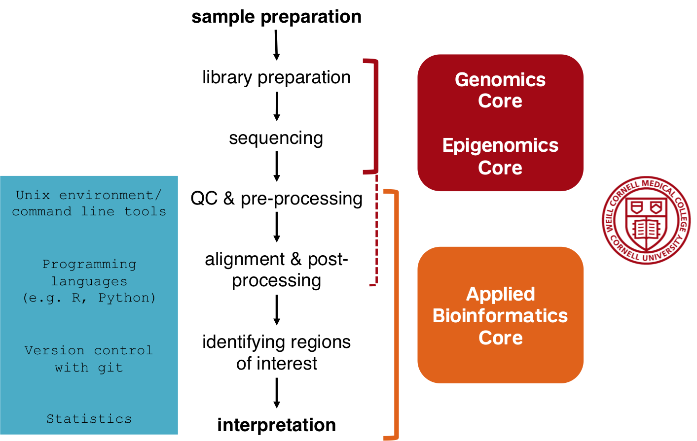
54 |
55 | We highly recommend to get in touch with the Core Facilities in order to work out the details of your own experiment.
56 | There are many parameters that can be tuned and optimized; the following paragraphs are meant to give you a brief glimpse into some of the major aspects that should be considered _before_ actually preparing your samples.
57 |
58 | The Epigenomics Core also compiled [detailed information](http://epicore.med.cornell.edu/services.php) about the different assays they're offering.
59 |
60 |
61 | ### Parameters to consider for the experiment
62 |
63 | Here are some of the most important things to think about:
64 |
65 | * appropriate control samples (e.g. input samples for ChIP-seq)
66 | * number of replicates
67 | * sequencing read length
68 | * paired-end sequencing or single reads
69 | * specific library preparations, e.g. poly-A enrichment vs. ribosomal depletion for RNA-seq, size range of the fragments to be amplified etc.
70 | * strand information is typically lost, but can be preserved it needed
71 |
72 | Typical problems of Illumina-based sequencing data are:
73 |
74 | * PCR artifacts such as duplicated fragments, lack of fragments with very high or very low GC content and biases towards shorter read lengths
75 | * sequencing errors and mis-identified bases
76 |
77 | These problems can be mitigated, but not completely eliminated, with careful library preparation (e.g., minimum numbers of PCR cycles, removal of excess primers) and frequent updates of Illumina's machines and chemistry.
78 |
79 | In addition, there are inherent limitations that are still not overcome:
80 |
81 | * short reads -- regions with lots of repetitive regions will be virtually impossible to see with typical read lengths of 100 bp
82 | * the data will most likely be only as good as the reference genome
83 | * statistical analysis of many applications has not caught up with the speed at which new assays are being developed -- gold standards of analysis exist for very few applications and many analyses are still hotly debated in the bioinformatics community (e.g., identification of broad histone mark enrichments, single cell RNA-seq analysis, isoform quantification, de novo transcript discovery (including lncRNA), ...)
84 |
85 | **There may be questions that are not best addressed with Illumina's sequencing platform!**
86 |
87 |
88 | ### How many and what types of replicates?
89 |
90 | For many HTS applications, the ultimate goal is to find the subset of regions or genes that show differences between the conditions that were analyzed. Conventional RNA-seq analysis, for example, can be used to interrogate thousands of genes at the same time, but the question you're asking for every gene is the same: is there a significant difference in expression between the two (or more) conditions?
91 |
92 | In order to be somewhat confident that the expression levels (or enrichment levels or methylation levels -- or whatever type of biological signal you were interested in) you're comparing are not just reflecting normal biological variation, but are indeed a consequence of the experimental condition, you will need to have more than one measurement per locus.
93 | Ideally, you should have hundreds of measurements, but practically, this will not be feasible due to financial and other constraints. You will therefore have to find a compromise between the number of samples you can afford to prepare and sequence and the number of samples you think you will need to gauge the variation in your system.
94 | The next figure illustrates how the assessment of a single locus (here called "Rando1A") changes depending on how many and which (!) samples were analyzed (note that all values come from the _same_ distribution that were arbitrarily assigned to either "sample type").
95 |
96 | 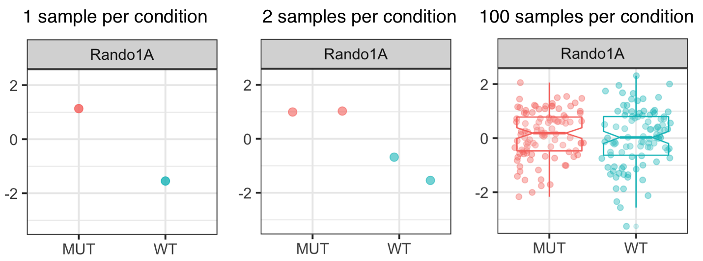
97 |
98 | **Technical replicates** are repeated measurements of the *same* sample.
99 | **Biological replicates** are parallel measurements of biologically *distinct* samples that capture random biological variation
100 |
101 | 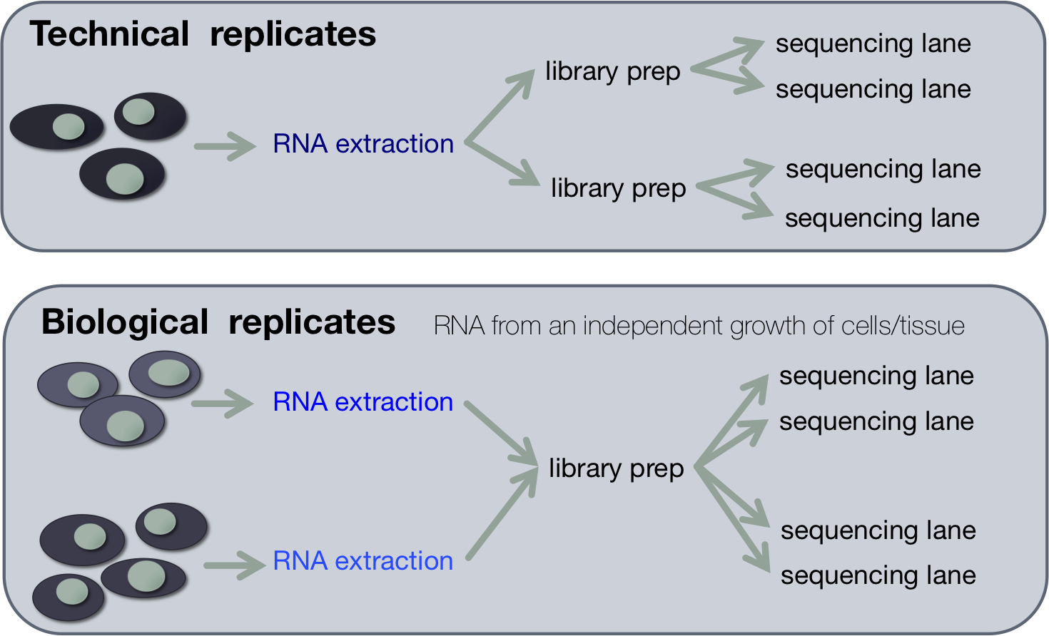
102 |
103 |
104 | ### Experimental design considerations
105 |
106 | The major rule is: **Block what you can, randomize what you cannot.**
107 | In practice, this means that you should try to keep the technical nuisance factors (e.g. cell harvest date, RNA/DNA extraction method, sequencing date, ...) to a minimum, i.e., try to be as consistent as possible. If you cannot harvest all the cells on the same day, make sure you do not confound parameters of interest with technical factors, i.e., absolutely avoid processing all, say, wild type samples on day 1 and all mutant samples on day 2.
108 |
109 | Don't overthink it (fully blocked design is simply not feasible), but make sure that the factors of interest are clear. This also means communicating with the sequencing facility about how to randomize technical variation appropriately and in accordance with your experiment's design.
110 | The classic paper by [Auer & Doerge](http://dx.doi.org/10.1534/genetics.110.114983) established the rules of balanced experimental design while leveraging the features of typical high-throughput DNA sequencing platforms.
111 | The following figure is taken from their paper:
112 |
113 | 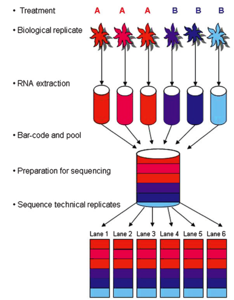
114 |
115 | For more details about experimental design considerations, see Section 1.4 of the [Introduction to RNA-seq](http://chagall.med.cornell.edu/RNASEQcourse/Intro2RNAseq.pdf), Altman N and Krzywinski M. (2014) [Nature Methods, 12(1):5–6, 2014](http://dx.doi.org/10.1038/nmeth.3224), and Blainey et al. (2014) [Nature Methods, 1(9) 879–880](https://www.nature.com/articles/nmeth.3091).
116 |
117 | For an enlightening read about how even seasoned genomics researchers can fall prey to inadvertend bias, [this paper](https://f1000research.com/articles/4-121/v1) including the comments and discussions is highly recommended.
118 |
119 |
120 | ## More resources
121 |
122 | WCM is part of a vibrant community of computational biologists and DNA sequencing experts!
123 |
124 |
125 | **Meetings**:
126 |
127 | Every Thursday, the Applied Bioinformatics Core offers a weekly [Bioinformatics Walk-in Clinic](https://abc.med.cornell.edu/ABC_Clinic.pdf) -- for all your questions about experimental design and data analysis!
128 |
129 | For more experienced coders and programmers, you may be interested to join the mailing list of [d:bug](https://github.com/abcdbug/dbug) to stay up-to-date with cool packages and state-of-the-art data science tips.
130 |
131 |
132 | **Classes**:
133 |
134 | * [Quantitative understanding in biology](http://physiology.med.cornell.edu/people/banfelder/qbio/) - review of quantitative techniques with an emphasis on how to select an appropriate statistical test, interpret the results, and design experiments
135 | * Workshops taught by personnel of the [Applied Bioinformatics Core](https://abc.med.cornell.edu):
136 | - Introduction to UNIX ([schedule](http://www.trii.org/courses/), [course notes](http://chagall.med.cornell.edu/UNIXcourse/))
137 | - Intro to differential gene expression analysis using RNA-seq ([schedule](http://www.trii.org/courses/), [course notes](http://chagall.med.cornell.edu/RNASEQcourse/) )
138 | - [Introduction to R](http://chagall.med.cornell.edu/Rcourse/intro2R.pdf)
139 | * [Genomics Workshop](http://weill.cornell.edu/ctsc/training_and_education/masters_degree_in_clinical.html) provided by the Genomics Resources Core Facility as part of the Master of Science in Clinical & Translational Investigation
140 |
141 |
142 | ### Self-paced reading and studying
143 |
144 | The Epigenomics Core has compiled [detailed information](http://epicore.med.cornell.edu/services.php) about the different types of -seq experiments they're performing.
145 |
146 | The [course notes](http://chagall.med.cornell.edu/RNASEQcourse/Intro2RNAseq.pdf) accompanying the Applied Bioinformatics Core's RNA-seq class contain a comprehensive introduction into many aspects of high-throughput sequencing data analysis.
147 |
148 | An introduction into general ChIP-seq analysis can be found [here](http://deeptools.readthedocs.io/en/latest/content/example_usage.html), including a [Glossary of HTS terms](http://deeptools.readthedocs.io/en/latest/content/help_glossary.html) including the different [file formats](http://deeptools.readthedocs.io/en/latest/content/help_glossary.html#file-formats).
149 |
150 | Benjamin Yakir's [Introduction to Statistics](http://pluto.huji.ac.il/~msby/StatThink/IntroStat.pdf) using lots of R and little calculus
151 |
152 | #### Online courses
153 |
154 | * Applied Bioinformatics Core's Datacamp Course [Introduction to R](https://www.datacamp.com/courses/abc-intro-2-r)
155 | * Applied Bioinformatics Core's [Introduction to version control using RStudio](https://www.datacamp.com/courses/abc-intro-2-git-in-rstudio)
156 | * Michael Love's [Intro to Computational Biology](https://biodatascience.github.io/compbio/)
157 |
158 | #### Articles
159 |
160 | * An excellent overview of the different sequencing techniques and applications: ["Coming of age: ten years of next- generation sequencing technologies"](http://dx.doi.org/10.1038/nrg.2016.49)
161 | * A good summary of sequencing platforms including publicly available data: ["High-throughput sequencing"](http://www.cell.com/molecular-cell/fulltext/S1097-2765(15)00340-8)
162 | * A very good read (including the reviews and comments) that discusses many scientific as well as ethical issues surrounding **batch effects** in data generated by sequencing consortia: https://f1000research.com/articles/4-121/v1
163 |
164 | * Nature Methods has compiled a great selection of brief introductions into many **statistical concepts** that biologists should be familiar with, such as p-value calculations, replicate handling, visualizations etc.: [Points of Significance Series](https://www.nature.com/collections/qghhqm/pointsofsignificance)
165 | * F1000Research has entire paper series ("gateways" or "channels") dedicated to specific topics, including data analyses using R: [Channels](https://f1000research.com/gateways)
166 |
167 | #### Community
168 |
169 | * [Biostars](https://www.biostars.org/)
170 | * [Seqanswers](http://seqanswers.com/forums/index.php)
171 |
--------------------------------------------------------------------------------
/microarrays.md:
--------------------------------------------------------------------------------
1 | Microarray analysis
2 | =====================
3 |
4 | * [MA Platforms](#platforms)
5 | * [File Formats](#fileformats)
6 | * [R packages](#packages)
7 | * [Normalizations](#norms)
8 | * [QC](#qc)
9 | * [Annotation with gene names](#anno)
10 | * [Tx cluster vs. probe set level](#difflevels)
11 | * [DE analysis](#de)
12 | * [Affymetrix proprietary software](#affy)
13 | * [Alternative splicing analysis](#alts)
14 | * [References](#refs)
15 |
16 | ---------------------------------
17 |
18 |
19 | There are two types of MA platforms:
20 |
21 | * spotted array -- 2 colors
22 | * 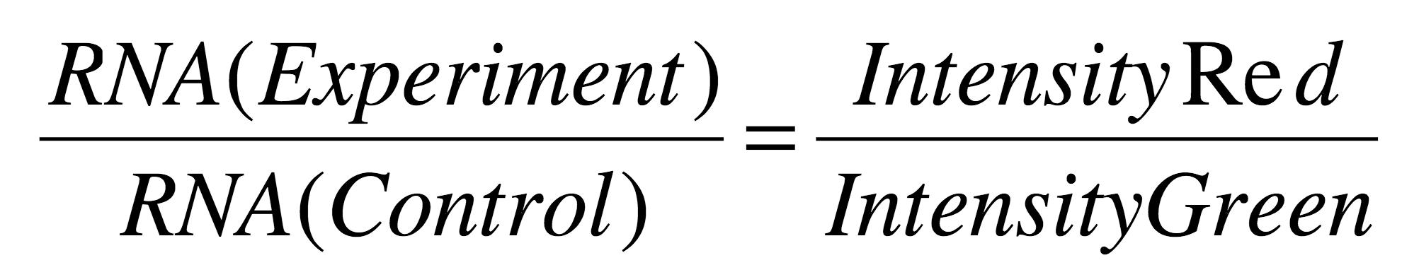
23 | * synthesized oligos -- 1 color (Affymetrix)
24 | * 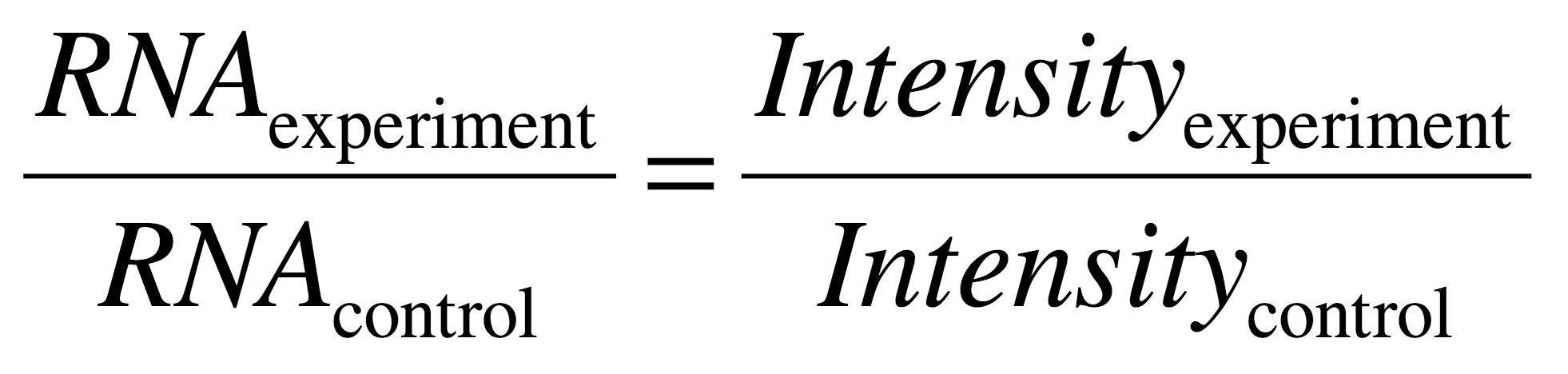
25 |
26 | We have: **GeneChip Human Transcriptome Array 2.0** (Affymetrix, now Thermo Scientific Fisher)
27 |
28 | * Gene Level plus Alternative Splicing
29 | * 70% exon probes, 30% exon-exon spanning probes
30 | * additional files and manuals provided by [Thermo Fisher](https://www.thermofisher.com/order/catalog/product/902162)
31 |
32 | Typically used microarrays:
33 |
34 | 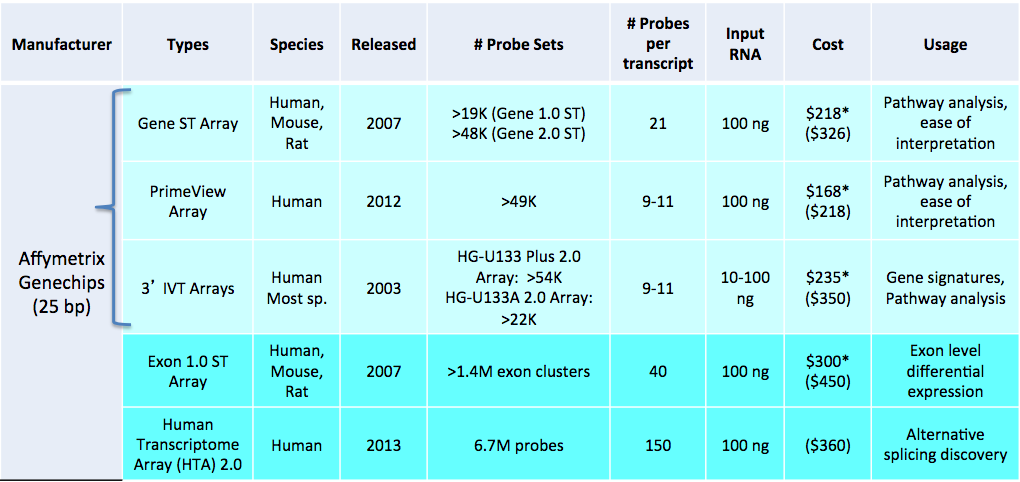
35 |
36 |
37 | ## File formats of microarrays
38 |
39 | * `.CEL`: Expression Array feature intensity
40 | * `.CDF`:
41 | - Chip definition file
42 | - information relating probe pair sets to locations on the array ("mapping" of the probe to a gene annotation)
43 | - in princple, these mappings can be updated
44 |
45 | 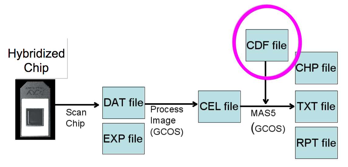
46 |
47 |
48 | ## Packages
49 |
50 | * `oligo`
51 | - supposed to replace `affy` for the more modern exon-based arrays
52 | - for data import and preprocessing
53 | - uses `ExpressionSet`
54 | - the best intro I found was the [github wiki](https://github.com/benilton/oligoOld/wiki/Getting-the-grips-with-the-oligo-Package)
55 |
56 | * `affy`
57 | - very comprehensive, but cannot read in HTA2.0 data
58 | - [affycoretools](https://github.com/Bioconductor-mirror/affycoretools/tree/master/R) has some functions to streamline array analysis, but they don't seem particularly fast
59 | - `arrayQualityMetrics` operates on `AffyBatch`
60 | * `xps`
61 | - uses `ROOT` to speed up storage and retrieval
62 | * `affyPLM`:
63 | - MAplot function will work on `ExpressionSet`
64 |
65 | ### Turning fluorescence signal into biological signal
66 |
67 | old MAs had mismatch probes to estimate the noise --> the RMA algorithm made those obsolete, so modern MAs only have perfect match (PM) probes
68 |
69 | **probeset** = group of probes covering one gene
70 |
71 | The data analyst can choose one from three definitions of probesets for summarization to the transcript level:
72 |
73 | 1. **Core Probesets**: supported by RefSeq and full-length mRNA GenBank records;
74 | 2. **Extended Probesets**: supported by non-full-length mRNA GenBank records, EST sequences, ENSEMBL gene collections and others;
75 | 3. **Full Probesets**: supported by gene and exon prediction algorithms only.
76 |
77 | Which one to use?
78 |
79 | 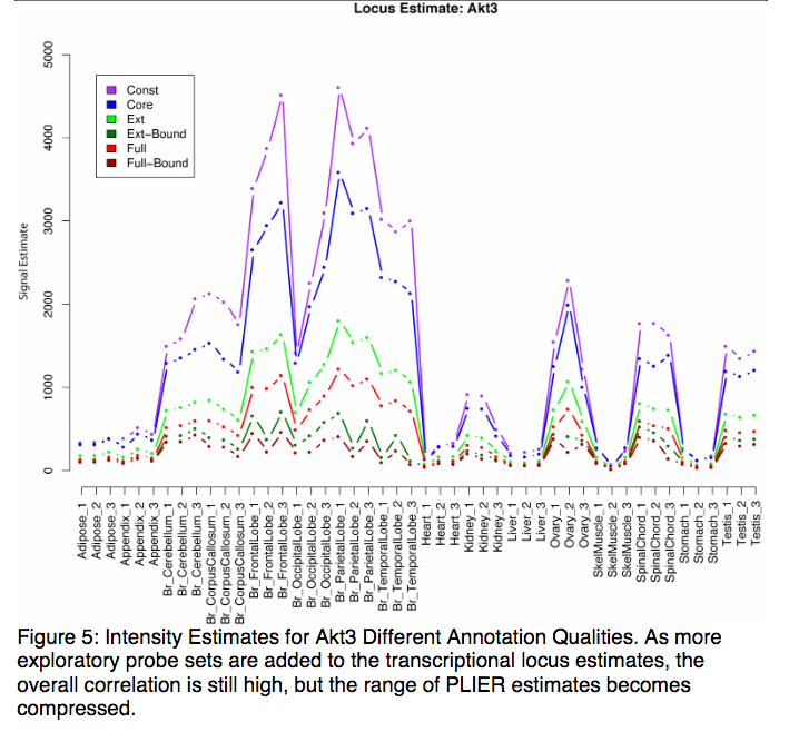
80 |
81 | > Each gene annotation is constructed from transcript annotations from one or more confidence levels. Some parts of a gene annotation may
82 | derive from high confidence core annotations, while other parts derive from the lower confidence extended or full annotations. [White Paper Probe Sets II](http://tools.thermofisher.com/content/sfs/brochures/exon_probeset_trans_clust_whitepaper.pdf)
83 |
84 |
85 | #### Normalization methods
86 |
87 | ##### MAS5
88 |
89 | basically subtracts out mismatch probes
90 |
91 | - Tukey's biweight estimator to provide robust mean signal, Wilcoxo rank test for p-value
92 | - bckg estimation: weighted average of the lowest 2% if the feature intensities
93 | - makes use of mismatch probes (applicable to HTA?)
94 | - linear scaling with trimmed mean
95 | - analyzes each array independently --> reduced power compared to the other methods
96 |
97 | info based on TAC User Manual, more details can be found in the slides of the [Canadian Bioinfo Workshop 2012, pages 5-7](http://bioinformatics.ca/files/public/Microarray_2012_Module2.pdf)
98 |
99 | ##### Robust Microarray Average (RMA)
100 |
101 | is a log scale linear additive model that uses only perfect match probes and extracts background mathematically (GCRMA additionally corrects for mismatch probes)
102 |
103 | _info from [Carvalho 2016](https://www.ncbi.nlm.nih.gov/pubmed/27008013), [RMA paper](https://www.ncbi.nlm.nih.gov/pubmed/12925520?access_num=12925520&link_type=MED)_
104 |
105 | Steps implemented in `rma()`:
106 |
107 | 1. Background adjustment
108 | - noise from cross-hybridization and optical noise from the scanning
109 | - remove _local_ artifacts so that measurements aren't so affected by their neighbors
110 | - bckg noise = normal distribution
111 | - true signal = exponential distribution that is probeset-specific
112 | 2. Quantile normalization
113 | - remove array-specific effects
114 | 3. Summarization --> obtaining expression levels
115 | - collapsing multiple probes per target into one signal
116 | - note that "probes" will be represented by background-adjusted, quantile-normalized, log-transformed PM intensities
117 | - 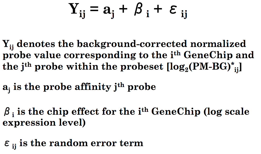
118 | - probe affinity a_j_ and chip effect beta_i_ must be estimated:
119 | - RMA default method: Tukey's Median Polish strategy (robust and fast, but no standard error estimates)
120 | - fits iteratively; successively removing row and column medians, and accumulating the terms until the process stabilizes; the residuals are what is left at the end
121 | - 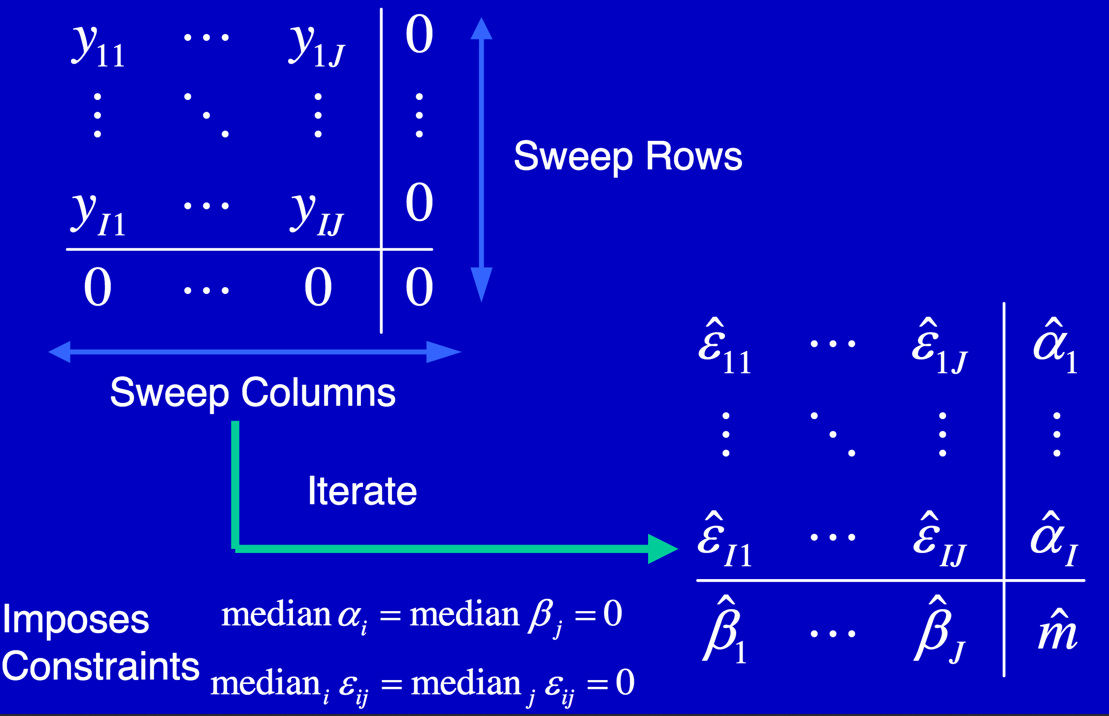
122 | - alternative: fitting a linear model (Probe Level Model, PLM)
123 | - 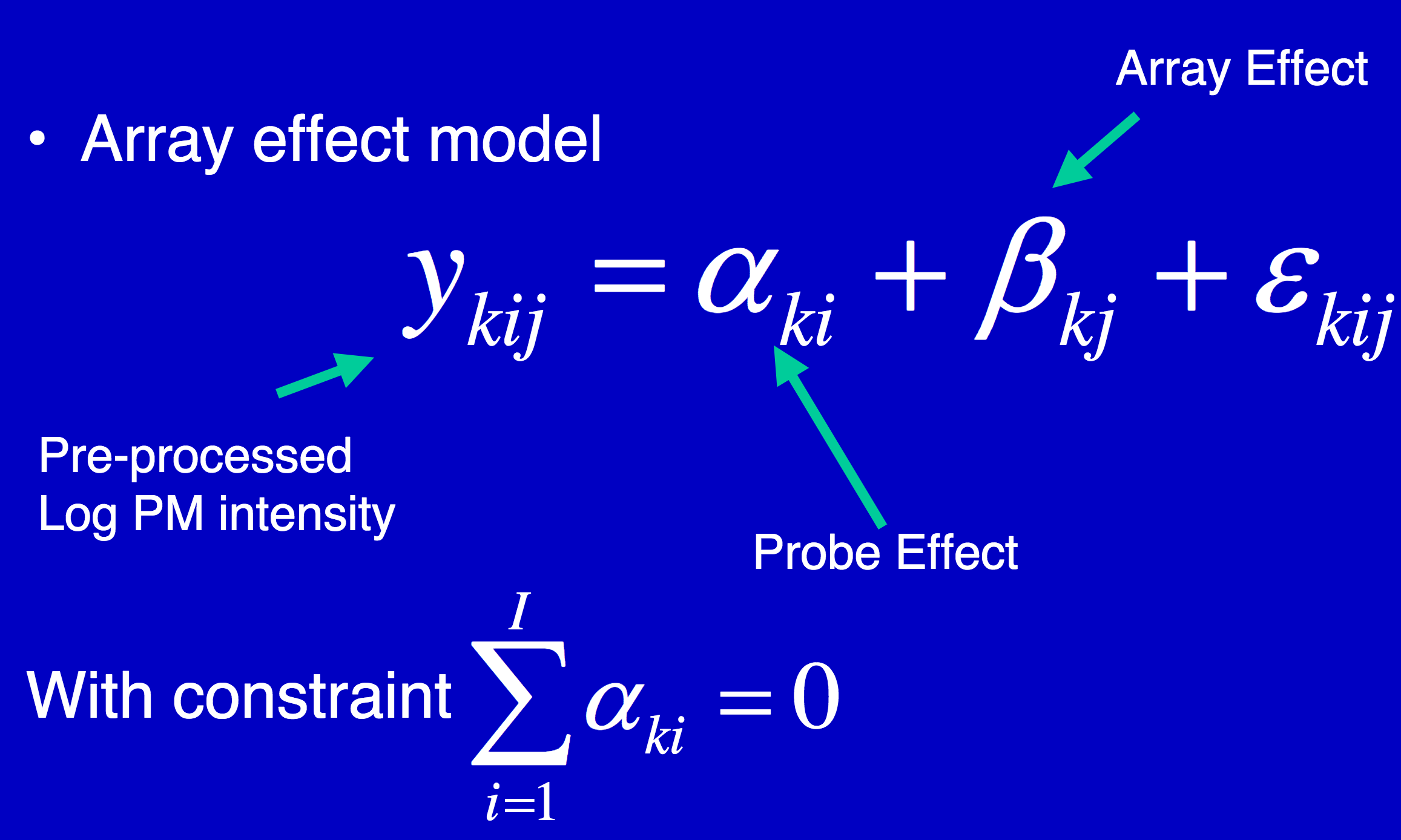
124 |
125 |
126 | 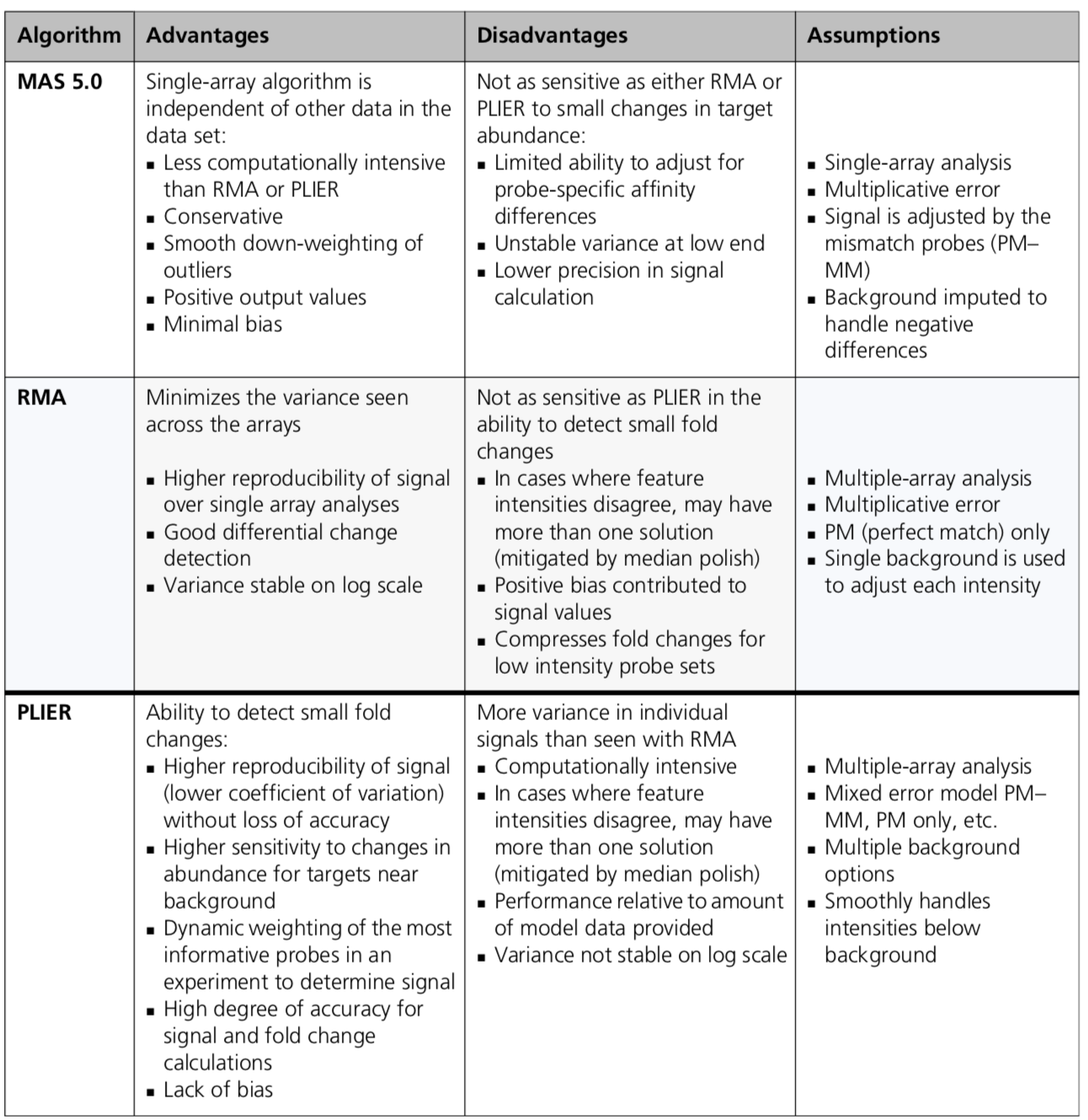
127 |
128 | PLIER is the proprietory (?) algorithm of Affymetrix/Thermo Fisher; Table taken from TAC Manual (Appendix)
129 |
130 | [White Paper Normalization](http://tools.thermofisher.com/content/sfs/brochures/sst_gccn_whitepaper.pdf) |
131 | [White Paper Probe Sets A](http://tools.thermofisher.com/content/sfs/brochures/exon_gene_signal_estimate_whitepaper.pdf) |
132 | [White Paper Probe Sets B](http://tools.thermofisher.com/content/sfs/brochures/exon_probeset_trans_clust_whitepaper.pdf)
133 |
134 |
135 | ## QC
136 |
137 | According to [McCall et al., 2011](https://bmcbioinformatics.biomedcentral.com/articles/10.1186/1471-2105-12-137), the most useful QC measures for identifying poorly performing arrays are:
138 |
139 | * RLE
140 | * NUSE
141 | * percent present
142 |
143 | ### Pseudo images
144 |
145 | Chip pseudo-images are very useful for detecting spatial differences (artifacts) on the invidual arrays (so not for comparing between arrays).
146 |
147 | Pseudo-images are generated by fitting a probe-level model (PLM) to the data that assumes that all probes of a probe set behave the same in the different samples: probes that bind well to their target should do so on all arrays, probes that bind with low affinity should do so on all arrays.
148 |
149 | You can create pseudo-images based on the residuals or the weights that result from a comparison of the model (the ideal data, without any noise) to the actual data. These weights or residuals may be graphically displayed using the `image()` function in Bioconductor (default: weights)
150 |
151 | The model consists of a probe level (assuming that each probe should behave the same on all arrays) and an array level (taking into account that a gene can have different expression levels in different samples) parameter.
152 |
153 | >info from [wiki.bits](http://wiki.bits.vib.be/index.php/How_to_create_chip_pseudo-images)
154 |
155 | ### Histograms of log2 intensity
156 |
157 | 
158 |
159 | ```
160 | for(i in 1:6){
161 | hist(data[,i],lwd=2,which='pm',ylab='Density',xlab='Log2ntensities',
162 | main=ph@data$sample[i])
163 | }
164 |
165 | # ggplot2 way
166 | pmexp = pm(data)
167 |
168 | ```
169 |
170 | ### Boxplots of log2 intensity per sample
171 |
172 | 
173 |
174 | `pmexp = log2(pm(data))`
175 |
176 | ### Boxplots of log2 intensity per GC probe
177 |
178 | 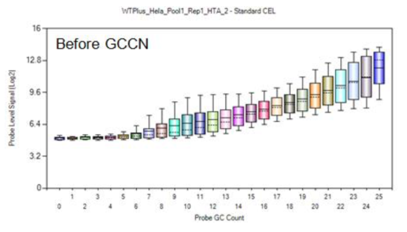
179 |
180 | ### MA plots
181 |
182 | MA plots were developed for two-color arrays to detect differences between the two color labels on the same array, and for these arrays they became hugely popular. This is why more and more people are now also using them for Affymetrix arrays but on Affymetrix only use a single color label. So people started using them to compare each Affymetrix array to a pseudo-array. The pseudo array consists of the median intensity of each probe over all arrays.
183 |
184 | The MA plot shows to what extent the variability in expression depends on the expression level (more variation on high expression values?). In an MA-plot, A is plotted versus M:
185 |
186 | - **M** = difference between the intensity of a probe on the array and the median intensity of that probe over all arrays
187 | - **A** = average of the intensity of a probe on that array and the median intesity of that probe over all arrays; `A = (logPMInt_array + logPMInt_medianarray)/2`
188 |
189 | 
190 |
191 | Ideally, the cloud of data points should be centered around M=0 (blue line). This is because we assume that the majority of the genes is not DE and that the number of upregulated genes is similar to the number of downregulated genes. Additionally, the variability of the M values should be similar for different A values (average intensities). You see that the spread of the cloud increases with the average intensity: the loess curve (red line) moves further and further away from M=0 when A increases. To remove (some of) this dependency, we will normalize the data.
192 |
193 | ```
194 | for (i in 1:6)
195 | {
196 | name = paste("MAplot",i,".jpg",sep="")
197 | jpeg(name)
198 | # MA-plots comparing the second array to the first array
199 | affyPLM::MAplot(eset.Dilution, which=c(1,2),ref=c(1,2),plot.method="smoothScatter")
200 | # if multiple ref are given, these samples will be used to calculate the median
201 | # equivalent: which=c("20A","20B"),ref=c("20A","20B")
202 | dev.off()
203 | }
204 | ```
205 |
206 | ### Relative expression boxplot (RLE)
207 |
208 | How much is the expression of a probe spread out relative to the same probe on other arrays?
209 |
210 | * large spread of RLE indicates large number of DE genes
211 | * Computed for each probeset by comparing the expression value
212 | on each array against the median expression value for that probeset across all arrays.
213 | * Ideally: most RLE values should be around zero.
214 | * does not depend on RMA model
215 |
216 | see `affyPLM`
217 |
218 | 
219 |
220 |
221 | ### Normalized unscaled standard error (NUSE)
222 |
223 | How much is the variability of probes within a gene spread out relative to probes of the same gene on other arrays?
224 |
225 | see affyPLM
226 |
227 | 
228 |
229 | ### QC stat plot
230 |
231 | see `simpleaffy` [documentation](https://www.rdocumentation.org/packages/simpleaffy/versions/2.48.0/topics/plot.qc.stats)
232 |
233 | | Parameter | Meaning |
234 | |-----------|---------|
235 | | x | A QCStats object |
236 | | fc.line.col | The colour to mark fold change lines with |
237 | |sf.ok.region | The colour to mark the region in which scale factors lie within appropriate bounds |
238 | | chip.label.col | The colour to label the chips with |
239 | |sf.thresh | Scale factors must be within this fold-range
240 | | gdh.thresh | Gapdh ratios must be within this range |
241 | | ba.thresh | beta actin must be within this range |
242 | |present.thresh | The percentage of genes called present must lie within this range |
243 | | bg.thresh | Array backgrounds must lie within this range |
244 | | label | What to call the chips |
245 | | main | The title for the plot |
246 | | usemid | If true use 3'/M ratios for the GAPDH and beta actin probes |
247 | |cex | Value to scale character size by (e.g. 0.5 means that the text should be plotted half size) |
248 | | ... | Other parameters to pass through to |
249 |
250 | 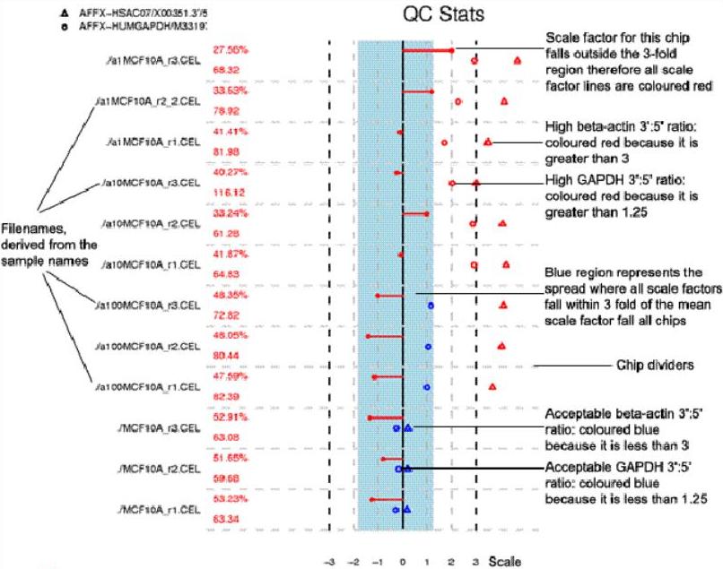
251 |
252 | * lines = arrays, from the 0-fold line to the point that corresponds to its MAS5 scale factor. Affymetrix recommend that scale factors should lie within 3-fold of each other.
253 |
254 | * points: GAPDH and beta-actin 3'/5' ratios. Affy states that beta actin should be within 3, gapdh around 1. Any that fall outside these thresholds (1.25 for gapdh) are coloured red; the rest are blue.
255 |
256 | * number of genes called present on each array vs. the average background. These will vary according to the samples being processed, and Affy's QC suggests simply that they should be similar. If any chips have significantly different values this is flagged in red, otherwise the numbers are displayed in blue. By default, 'significant' means that %-present are within 10% of each other; background intensity, 20 units. These last numbers are somewhat arbitrary and may need some tweaking to find values that suit the samples you're dealing with, and the overall nature of your setup.
257 |
258 | * BioB = spike-in; if not present on a chip, this will be flagged by printing 'BioB' in red; this is a control for the hybridization step
259 |
260 |
261 | ### Source of variation
262 |
263 | which attribute explains most of the variation ([page 82f.](https://assets.thermofisher.com/TFS-Assets/LSG/manuals/tac_user_manual.pdf))
264 |
265 | Determine the fraction of the total variation of the samples can be explained by a given attribute:
266 |
267 | 1. compute variance of each probeset
268 | 2. retain the 1000 probesets having the highest variance
269 | 3. Accumulate the _total sum of squares_ for each attribute
270 | 4. The _residual sum of squares_ (where the sum over j represents the sum over samples within the attribute level) is accumulated.
271 | 5. The fraction of variance explained for the attribute is the _mean of the fraction explained_ over all of the probesets.
272 |
273 |
274 | ## Annotating probes with gene names
275 |
276 | Thermo Fisher provides data bases with the mappings [here](https://www.thermofisher.com/us/en/home/life-science/microarray-analysis/microarray-data-analysis/genechip-array-annotation-files.html)
277 |
278 | [Annotation Dbi](https://www.bioconductor.org/packages/devel/bioc/vignettes/AnnotationDbi/inst/doc/IntroToAnnotationPackages.pdf) seems to be the native R way to do this.
279 |
280 | For an overview of all bioconductor-hosted annotation data bases, see [here](http://www.bioconductor.org/packages/release/BiocViews.html#___AnnotationData).
281 | For HTA2.0, there are two options: [transcript clusters](http://www.bioconductor.org/packages/release/data/annotation/manuals/hta20transcriptcluster.db/man/hta20transcriptcluster.db.pdf) and [probe sets](http://www.bioconductor.org/packages/release/data/annotation/manuals/hta20probeset.db/man/hta20probeset.db.pdf)
282 |
283 |
284 | * __probe sets__: for HTA2.0, a probe set is more are less an exon, but not quite
285 | - old Exon ST arrays had four-probe probesets (e.g., four 25-mers that were summarized to estimate the expression of a 'probe set region', or PSR). A PSR was some or all of an exon, so it wasn't even that clear what you were measuring. If the exon was long, there might have been multiple PSRs for the exon, or if it was short maybe only one.
286 | - when you summarize at the probeset level on the HTA arrays, you are summarizing all the probes in a probeset, which may measure a PSR, or may also summarize a set of probes that are supposed to span an exon-exon junction
287 | - analyzing the data at this level is very complex: any significantly differentially expressed PSR or JUC (junction probe) just says something about a little chunk of the gene, and what that then means in the larger context of the gene is something that you have to explore further.
288 | * __transcript clusters__: contain all probe sets of a _transcript_
289 | - there may be multiple transcript probesets for a given gene
290 | - given the propensity for Affy to re-use probes in the later versions of arrays, the multiple probesets for a given gene may well include some of the same probes!
291 | - the transcript level probesets provide some relative measure of the underlying transcription level of a gene
292 | - different probesets for the same gene may measure different splice variants.
293 |
294 | [Ref1](https://www.biostars.org/p/12180/),
295 | [Ref2](https://support.bioconductor.org/p/89308/)
296 |
297 | [Stephen Turner](http://www.statsblogs.com/2012/01/17/annotating-limma-results-with-gene-names-for-affy-microarrays/) has a blog entry on how to do the annotation before the limma analysis; he uses transcript clusters (= gene-level analysis)
298 |
299 |
300 | ## DE Analysis
301 |
302 | A very good summary of all the most important steps is given by [James MacDonald at biostars](https://support.bioconductor.org/p/89308/).
303 |
304 | ```
305 | library(oligo)
306 | dat <- read.celfiles(list.celfiles())
307 | eset <- rma(dat)
308 |
309 | ## you can then get rid of background probes and annotate using functions in my affycoretools package
310 | library(affycoretools)
311 | library(hta20transcriptcluster.db)
312 | eset.main <- getMainProbes(eset, pd.hta.2.0)
313 | eset.main <- annotateEset(eset.main, hta20stranscriptcluster.db)
314 | ```
315 |
316 | For probe-set level analysis (see caveats above!):
317 |
318 | ```
319 | eset <- rma(dat, target = "probeset")
320 | eset.main <- getMainProbes(eset, pd.hta.2.0)
321 | eset.main <- annotateEset(eset.main, hta20probeset.db)
322 | ```
323 |
324 | -----------------------------------------------
325 |
326 |
327 | ## Affymetrix' TAC
328 |
329 | * Affymetrix' software (Windows only)
330 | - [User manual](https://assets.thermofisher.com/TFS-Assets/LSG/manuals/tac_user_manual.pdf)
331 | * uses the following R packages:
332 | - [Apcluster](https://dx.doi.org/10.1093/bioinformatics/btr406) - affinity propagation clustering
333 | - [Dbscan](https://CRAN.R-project.org/package=dbscan) - density based clustering of applications with noise
334 | - Rtsne
335 | - limma
336 | * offers the following __normalization methods__:
337 | - RMA
338 | - MAS5
339 | - Plier PM-MM
340 | * __QC__:
341 | - [Thermo Fisher White Paper](http://tools.thermofisher.com/content/sfs/brochures/exon_gene_arrays_qa_whitepaper.pdf)
342 | - PCA
343 |
344 |
345 | ## Alternative splicing
346 |
347 | - **EventPointer**
348 | - [R vignette](https://bioconductor.org/packages/release/bioc/vignettes/EventPointer/inst/doc/EventPointer.html)
349 | - [original paper]()
350 | - [code at github](https://github.com/jpromeror/EventPointer)
351 | - [Example Data](https://www.dropbox.com/sh/wpwz1jx0l112icw/AAD4yrEY4HG1fExUmtoBmrOWa/HTA%202.0?dl=0) including GTF file
352 |
353 |
354 |
355 | ## References
356 |
357 | * [JR Stevens 2012](www.math.usu.edu/~jrstevens/stat5570/1.4.Preprocess.pdf)
358 | * [Canadian Bioinfo Workshop on Microarrays](https://bioinformatics.ca/workshops/2012/microarray-data-analysis)
359 |
--------------------------------------------------------------------------------