├── README.md
├── faq
├── GATK workshop的变异寻找流程.md
├── GATK的学习小组包括哪些内容呢.md
├── GATK软件需要的输入文件是哪些.md
├── 参加GATK的研讨会操作课程前需要准备什么.md
└── 如何向GATK官方汇报bugs.md
├── methods
├── 基于DNAseq的GATK最佳实践概述.md
├── 基于RNAseq的GATK最佳实践概述.md
└── 基于RNAseq的GATK最佳实践流程.md
├── processing.md
└── tutorials
├── .DS_Store
├── filetype
├── 从vcf格式的变异文件里面挑选感兴趣位点.md
├── 如何不比对就把fastq文件转为bam格式呢?.md
├── 如何从fasta序列里面模拟测序reads?.md
├── 如何处理参考基因组的非染色体序列?.md
├── 如何对bam文件进行修复.md
└── 如何根据坐标区间对bam文件取子集?.md
├── steps
├── 如何去除PCR重复?.md
├── 如何用HC找变异.md
├── 如何用UG找变异.md
├── 如何运行BQSR.md
├── 如何运行VQSR.md
└── 如何高效的比对?.md
├── vcf-filter-annotation
├── .DS_Store
├── GVCF和普通的VCF文件的区别是什么.md
├── VCF文件是什么,该如何解释呢.md
├── 变异位点评价模块是干什么的.md
├── 如何对vcf文件进行过滤?.md
├── 用CollectVariantCallingMetrics来评价找到的变异.md
├── 用VariantEval来评价找到的变异.md
├── 突变碱基特异性注释和过滤.md
└── 评价找到的变异.md
└── 如何安装GATK最佳实践的必备软件.md
/README.md:
--------------------------------------------------------------------------------
1 | # GATK中文社区招募
2 |
3 | 昨天gatk官网放出了征求中文社区合作伙伴的消息,作为生物信息学领域最活跃的中文社群,我们当仁不让的要接下这茬。GATK流程是目前科研界+工业界应用最广泛变异位点识别流程,而且是由大名鼎鼎的broad开发和维护,非常具有学习参考价值。
4 |
5 | 首先介绍一下我们的计划:
6 |
7 | ## 建设协作论坛
8 |
9 | 采用开源论坛系统Flarum建设GATK中文社区,该论坛所有帖子将以markdown代码形式发帖,所有的markdown源代码都会同步存放在此github的organization的这个project下面。GATK中文社区地址是: 对应的broad的GATK主页是;
10 |
11 | ## 建设协作github
12 |
13 | 因为论坛都是以markdown写作,所以源代码很容易上传保存到统一的github合作仓库。https://github.com/gatk-chinese/forum
14 |
15 | - faq
16 | - tools
17 | - tutorials
18 | - methods
19 | - others
20 | - Images (存储上面5个文件夹的所有图片)
21 |
22 | 下面介绍一下GATK官方的工作,我们在github建立的5个存放markdown源代码的文件夹,对应着下面的GATK官网的5块知识点。
23 |
24 | ## 文档
25 |
26 | - 约40多个最常见的用户问题[Frequently Asked Questions ](https://software.broadinstitute.org/gatk/documentation/topic?name=faqs)
27 | - 约30多个官方教程[Step-by-step instructions targeted by use case](https://software.broadinstitute.org/gatk/documentation/topic?name=tutorials)
28 | - 约20多个[专有名词解释](https://software.broadinstitute.org/gatk/documentation/topic?name=dictionary)
29 | - 一些PPT和[youtube视频下载](https://software.broadinstitute.org/gatk/documentation/presentations) 存放在 the [GATK Workshops](https://drive.google.com/open?id=1y7q0gJ-ohNDhKG85UTRTwW1Jkq4HJ5M3) directory 需要翻墙!
30 |
31 | 这个工作量是最大的,需要**GATK熟手**才能比较流畅的翻译加工。我已经在自己的社交圈物色了3名不错的人才负责这部分知识点,同时也欢迎读者推荐自己或者认识的高手加盟,我会认真对待这个合作。
32 |
33 | ## 套件的工具
34 |
35 | GATK涉及到了对高通量测序数据寻找遗传变异位点过程的方方面面,绝大部分用户用到了就是GATK对bam文件的一个再处理,还有UG或者HC模式的变异寻找工具。
36 |
37 | - [Diagnostics and Quality Control Tools](https://software.broadinstitute.org/gatk/documentation/tooldocs/current/#DiagnosticsandQualityControlTools)
38 | - [Sequence Data Processing Tools](https://software.broadinstitute.org/gatk/documentation/tooldocs/current/#SequenceDataProcessingTools)
39 | - [Variant Discovery Tools](https://software.broadinstitute.org/gatk/documentation/tooldocs/current/#VariantDiscoveryTools)
40 | - [Variant Evaluation Tools](https://software.broadinstitute.org/gatk/documentation/tooldocs/current/#VariantEvaluationTools)
41 | - [Variant Manipulation Tools](https://software.broadinstitute.org/gatk/documentation/tooldocs/current/#VariantManipulationTools)
42 |
43 | 这个主要是工具的帮助文档的翻译,理论上谷歌翻译+人工修改就可以了,并没有涉及到过多的生物信息学知识点,对**经验要求也不高**,大部分都是工具的参数的解读。这个版块需要比较多的志愿者参与,欢迎联系我邮箱 jmzeng1314@163.com 获取参与细节,来信请务必做好一定程度的自我介绍。
44 |
45 | ## 用法及算法
46 |
47 | 这个版块与其官方教程部分重叠,但是侧重于对步骤细节的理解以及取舍,对变异位点识别原理的掌握要求也很高。目前处于待定状态,可能需要专家加盟,甚至需要部分从事遗传咨询研究的朋友合作翻译,而不仅仅是做数据处理的生物信息学家。
48 |
49 | ## [最佳实践](https://software.broadinstitute.org/gatk/best-practices/)
50 |
51 | 这里准备结合几个项目数据分析实际案例来讲解如何应用GATK官网推荐的最佳流程。
52 |
53 | ## [博客](https://software.broadinstitute.org/gatk/blog)
54 |
55 | 主要是GATK官方维护小组的人会在上面发布一些关于GATK的动态,版本,小故事,会议等等。并不在我们的翻译计划中。
56 |
57 | ## [论坛](https://gatkforums.broadinstitute.org/gatk)
58 |
59 | 这里有全世界各地不同生物信息学水平的遗传变异研究者对于GATK,但不限于该软件使用方法的各种讨论。目前也不在我们的翻译计划中。
60 |
--------------------------------------------------------------------------------
/faq/GATK的学习小组包括哪些内容呢.md:
--------------------------------------------------------------------------------
1 | # GATK的研讨会包括哪些内容呢?
2 |
3 | 原文链接:[ What do GATK workshops cover?](https://software.broadinstitute.org/gatk/documentation/article?id=9218)
4 |
5 | ## 为期三天的GATK研讨会
6 |
7 | 这次研讨会将会集中在使用broad研究所开发的GATK软件来寻找变异位点的核心步骤,即GATK小组开发的最佳实践流程。你将会了解为什么最佳实践的每个步骤都是寻找变异位点这一过程必不可少的,每一步骤分别对数据做了什么,如何使用GATK工具来处理你自己的数据并得到最可信最准确的结果。同时,在研讨会的课程中,我们会突出讲解部分GATK的新功能,比如用GVCF模式来对多样本联合寻找变异,还有如何对RNA-seq数据特异的寻找变异流程,和如何使用mutech2来选择somatic变异。我们也会介绍一下即将到来的GATK4的功能,比如它的CNV流程。最后我们会演练整个GATK流程的各个步骤的衔接和实战。
8 |
9 | ## 课程设置
10 |
11 | 本次研讨会包括一天的讲座,中间会提供大量的问答环节,力图把GATK的基础知识介绍给大家。并且伴随着2天的上机实战,具体安排如下:
12 |
13 | - 第一天全天:演讲,关于GATK最佳实践应用于高通量测序数据的前因后果,理论基础以及应用形式。
14 | - 第二天上午:上机操作, 使用GATK寻找变异位点,包括(SNPs + Indels)
15 | - 第二天下午:上机操作,使用GATK对找到变异位点进行过滤。
16 | - 第三天上午:上机操作,使用GATK寻找somatic的变异位点,包括 (SNPs + Indels + CNV)
17 | - 第三天下午:介绍通过WDL(Workflow Description Language)整合的云端流程
18 |
19 | 上机实践侧重于数据分析步骤,希望提供练习的方式帮助用户了解寻找变异位点这一过程中涉及到的各种文件格式的转换,以及如何更好的利用GATK工具来完成这一流程。在这些实践课程中,我们会有机的结合GATK和PICARDS工具,还有其它一些第三方工具,比如Samtools, IGV, RStudio and RTG Tools ,介绍它们的一些操作技巧,比较有趣的分析方法,还有中间可能会遇到的报错信息的处理。
20 |
21 | 还会讲解如何使用WDL来写GATK分析流程的脚本,这个是broad最新开发的一个流程描述语言。并且在本地或者云端执行自己写好的流程。
22 |
23 | 请注意,本次研讨会侧重于人类研究数据的处理,本次研究会讲解的大部分操作步骤都适合其它非人类研究数据的处理,但是应用起来会有一些需要解决的移植问题,不过在这一点上面我们不会讲太多。
24 |
25 | ## 目标受众
26 |
27 | 第一天的基础知识讲解的受众比较广泛,既可以是第一次接触变异位点寻找这个分析方法,或者第一次接触GATK,想从零开始了解;也可以是已经使用过GATK的用户,想提升自己对GATK的理解。但是参会者需要熟练一些基础名词,并且有基因组或者遗传学的基本背景。
28 |
29 | 上机操作是为那些想了解GATK具体使用过程的细节新手或者中级用户准备的,需要对LINUX命令行有着基础的理解能力。希望参会者可以带自己的笔记本电脑,并且预先安装好一些必备的软件工具,具体细节将会在研究会正式开始前两周公布,除非研究会的举办方提供了练习用的电脑或者云服务器。而且必须是mac或者linux系统,Windows系统是不能参加上机实践的。限30人!
30 |
31 | ## GATK最佳实践的PPT演讲内容如下:
32 |
33 | - Introduction to variant discovery analysis and GATK Best Practices
34 | - (coffee break)
35 | - Marking Duplicates
36 | - Indel Realignment (to be phased out)
37 | - Base Recalibration
38 | - (lunch break)
39 | - Germline Variant Calling and Joint Genotyping
40 | - Filtering germline variants with VQSR
41 | - Genotype Refinement Workflow
42 | - (coffee break)
43 | - Callset Evaluation
44 | - Somatic variant discovery with MuTect2
45 | - Preview of CNV discovery with GATK4
--------------------------------------------------------------------------------
/faq/GATK软件需要的输入文件是哪些.md:
--------------------------------------------------------------------------------
1 | # GATK软件需要的输入文件是哪些?
2 |
3 | 原文链接:[ What input files does the GATK accept / require? ](https://software.broadinstitute.org/gatk/documentation/article?id=1204)
4 |
5 | All analyses done with the GATK typically involve several (though not necessarily all) of the following inputs:
6 |
7 | - Reference genome sequence
8 | - Sequencing reads
9 | - Intervals of interest
10 | - Reference-ordered data
11 |
12 | This article describes the corresponding file formats that are acceptable for use with the GATK.
13 |
14 | ------
15 |
16 | ### 1. Reference Genome Sequence
17 |
18 | The GATK requires the reference sequence in a single reference sequence in FASTA format, with all contigs in the same file. The GATK requires strict adherence to the FASTA standard. All the standard IUPAC bases are accepted, but keep in mind that non-standard bases (i.e. other than ACGT, such as W for example) will be ignored (i.e. those positions in the genome will be skipped).
19 |
20 | **Some users have reported having issues with reference files that have been stored or modified on Windows filesystems. The issues manifest as "10" characters (corresponding to encoded newlines) inserted in the sequence, which cause the GATK to quit with an error. If you encounter this issue, you will need to re-download a valid master copy of the reference file, or clean it up yourself.**
21 |
22 | Gzipped fasta files will not work with the GATK, so please make sure to unzip them first. Please see [this article](http://www.broadinstitute.org/gatk/guide/article?id=1601) for more information on preparing FASTA reference sequences for use with the GATK.
23 |
24 | #### Important note about human genome reference versions
25 |
26 | If you are using human data, your reads must be aligned to one of the official b3x (e.g. b36, b37) or hg1x (e.g. hg18, hg19) references. The names and order of the contigs in the reference you used must exactly match that of one of the official references canonical orderings. These are defined by historical karotyping of largest to smallest chromosomes, followed by the X, Y, and MT for the b3x references; the order is thus 1, 2, 3, ..., 10, 11, 12, ... 20, 21, 22, X, Y, MT. The hg1x references differ in that the chromosome names are prefixed with "chr" and chrM appears first instead of last. The GATK will detect misordered contigs (for example, lexicographically sorted) and throw an error. This draconian approach, though unnecessary technically, ensures that all supplementary data provided with the GATK works correctly. You can use ReorderSam to fix a BAM file aligned to a missorted reference sequence.
27 |
28 | **Our Best Practice recommendation is that you use a standard GATK reference from the GATK resource bundle.**
29 |
30 | ------
31 |
32 | ### 2. Sequencing Reads
33 |
34 | The only input format for sequence reads that the GATK itself supports is the [Sequence Alignment/Map (SAM)] format. See [SAM/BAM] for more details on the SAM/BAM format as well as [Samtools](http://samtools.sourceforge.net/) and [Picard](http://picard.sourceforge.net/), two complementary sets of utilities for working with SAM/BAM files.
35 |
36 | If you don't find the information you need in this section, please see our [FAQs on BAM files](http://www.broadinstitute.org/gatk/guide/article?id=1317).
37 |
38 | If you are starting out your pipeline with raw reads (typically in FASTQ format) you'll need to make sure that when you map those reads to the reference and produce a BAM file, the resulting BAM file is fully compliant with the GATK requirements. See the Best Practices documentation for detailed instructions on how to do this.
39 |
40 | In addition to being in SAM format, we require the following additional constraints in order to use your file with the GATK:
41 |
42 | - The file must be binary (with `.bam` file extension).
43 | - The file must be indexed.
44 | - The file must be sorted in coordinate order with respect to the reference (i.e. the contig ordering in your bam must exactly match that of the reference you are using).
45 | - The file must have a proper bam header with read groups. Each read group must contain the platform (PL) and sample (SM) tags. For the platform value, we currently support 454, LS454, Illumina, Solid, ABI_Solid, and CG (all case-insensitive).
46 | - Each read in the file must be associated with exactly one read group.
47 |
48 | Below is an example well-formed SAM field header and fields (with @SQ dictionary truncated to show only the first two chromosomes for brevity):
49 |
50 | ```
51 | @HD VN:1.0 GO:none SO:coordinate
52 | @SQ SN:1 LN:249250621 AS:NCBI37 UR:file:/lustre/scratch102/projects/g1k/ref/main_project/human_g1k_v37.fasta M5:1b22b98cdeb4a9304cb5d48026a85128
53 | @SQ SN:2 LN:243199373 AS:NCBI37 UR:file:/lustre/scratch102/projects/g1k/ref/main_project/human_g1k_v37.fasta M5:a0d9851da00400dec1098a9255ac712e
54 | @RG ID:ERR000162 PL:ILLUMINA LB:g1k-sc-NA12776-CEU-1 PI:200 DS:SRP000031 SM:NA12776 CN:SC
55 | @RG ID:ERR000252 PL:ILLUMINA LB:g1k-sc-NA12776-CEU-1 PI:200 DS:SRP000031 SM:NA12776 CN:SC
56 | @RG ID:ERR001684 PL:ILLUMINA LB:g1k-sc-NA12776-CEU-1 PI:200 DS:SRP000031 SM:NA12776 CN:SC
57 | @RG ID:ERR001685 PL:ILLUMINA LB:g1k-sc-NA12776-CEU-1 PI:200 DS:SRP000031 SM:NA12776 CN:SC
58 | @PG ID:GATK TableRecalibration VN:v2.2.16 CL:Covariates=[ReadGroupCovariate, QualityScoreCovariate, DinucCovariate, CycleCovariate], use_original_quals=true, defau
59 | t_read_group=DefaultReadGroup, default_platform=Illumina, force_read_group=null, force_platform=null, solid_recal_mode=SET_Q_ZERO, window_size_nqs=5, homopolymer_nback=7, except on_if_no_tile=false, pQ=5, maxQ=40, smoothing=137 UR:file:/lustre/scratch102/projects/g1k/ref/main_project/human_g1k_v37.fasta M5:b4eb71ee878d3706246b7c1dbef69299
60 | @PG ID:bwa VN:0.5.5
61 | ERR001685.4315085 16 1 9997 25 35M * 0 0 CCGATCTCCCTAACCCTAACCCTAACCCTAACCCT ?8:C7ACAABBCBAAB?CCAABBEBA@ACEBBB@? XT:A:U XN:i:4 X0:i:1 X1:i:0 XM:i:2 XO:i:0 XG:i:0 RG:Z:ERR001685 NM:i:6 MD:Z:0N0N0N0N1A0A28 OQ:Z:>>:>2>>>>>>>>>>>>>>>>>>?>>>>??>???>
62 | ERR001689.1165834 117 1 9997 0 * = 9997 0 CCGATCTAGGGTTAGGGTTAGGGTTAGGGTTAGGG >7AA<@@C?@?B?B??>9?B??>A?B???BAB??@ RG:Z:ERR001689 OQ:Z:>:<<8<<<><<><><<>7<>>>?>>??>???????
63 | ERR001689.1165834 185 1 9997 25 35M = 9997 0 CCGATCTCCCTAACCCTAACCCTAACCCTAACCCT 758A:?>>8?=@@>>?;4<>=??@@==??@?==?8 XT:A:U XN:i:4 SM:i:25 AM:i:0 X0:i:1 X1:i:0 XM:i:2 XO:i:0 XG:i:0 RG:Z:ERR001689 NM:i:6 MD:Z:0N0N0N0N1A0A28 OQ:Z:;74>7><><><>>>>><:<>>>>>>>>>>>>>>>>
64 | ERR001688.2681347 117 1 9998 0 * = 9998 0 CGATCTTAGGGTTAGGGTTAGGGTTAGGGTTAGGG 5@BA@A6B???A?B??>B@B??>B@B??>BAB??? RG:Z:ERR001688 OQ:Z:=>>>><4><
45 | ```
46 |
47 | 2) Alignment jobs were executed as follows:
48 |
49 | ```
50 | runDir=/path/to/1pass
51 | mkdir $runDir
52 | cd $runDir
53 | STAR --genomeDir $genomeDir --readFilesIn mate1.fq mate2.fq --runThreadN
54 | ```
55 |
56 | 3) For the 2-pass STAR, a new index is then created using splice junction information contained in the file SJ.out.tab from the first pass:
57 |
58 | ```
59 | genomeDir=/path/to/hg19_2pass
60 | mkdir $genomeDir
61 | STAR --runMode genomeGenerate --genomeDir $genomeDir --genomeFastaFiles hg19.fa \
62 | --sjdbFileChrStartEnd /path/to/1pass/SJ.out.tab --sjdbOverhang 75 --runThreadN
63 | ```
64 |
65 | 4) The resulting index is then used to produce the final alignments as follows:
66 |
67 | ```
68 | runDir=/path/to/2pass
69 | mkdir $runDir
70 | cd $runDir
71 | STAR --genomeDir $genomeDir --readFilesIn mate1.fq mate2.fq --runThreadN
72 | ```
73 |
74 | #### 2. Add read groups, sort, mark duplicates, and create index
75 |
76 | The above step produces a SAM file, which we then put through the usual Picard processing steps: adding read group information, sorting, marking duplicates and indexing.
77 |
78 | ```
79 | java -jar picard.jar AddOrReplaceReadGroups I=star_output.sam O=rg_added_sorted.bam SO=coordinate RGID=id RGLB=library RGPL=platform RGPU=machine RGSM=sample
80 |
81 | java -jar picard.jar MarkDuplicates I=rg_added_sorted.bam O=dedupped.bam CREATE_INDEX=true VALIDATION_STRINGENCY=SILENT M=output.metrics
82 | ```
83 |
84 | #### 3. Split'N'Trim and reassign mapping qualities
85 |
86 | Next, we use a new GATK tool called SplitNCigarReads developed specially for RNAseq, which splits reads into exon segments (getting rid of Ns but maintaining grouping information) and hard-clip any sequences overhanging into the intronic regions.
87 |
88 | In the future we plan to integrate this into the GATK engine so that it will be done automatically where appropriate, but for now it needs to be run as a separate step.
89 |
90 | At this step we also add one important tweak: we need to reassign mapping qualities, because STAR assigns good alignments a MAPQ of 255 (which technically means “unknown” and is therefore meaningless to GATK). So we use the GATK’s [ReassignOneMappingQuality](http://www.broadinstitute.org/gatk/gatkdocs/org_broadinstitute_sting_gatk_filters_ReassignOneMappingQualityFilter.html) read filter to reassign all good alignments to the default value of 60. This is not ideal, and we hope that in the future RNAseq mappers will emit meaningful quality scores, but in the meantime this is the best we can do. In practice we do this by adding the ReassignOneMappingQuality read filter to the splitter command.
91 |
92 | Finally, be sure to specify that reads with N cigars should be allowed. This is currently still classified as an "unsafe" option, but this classification will change to reflect the fact that this is now a supported option for RNAseq processing.
93 |
94 | ```
95 | java -jar GenomeAnalysisTK.jar -T SplitNCigarReads -R ref.fasta -I dedupped.bam -o split.bam -rf ReassignOneMappingQuality -RMQF 255 -RMQT 60 -U ALLOW_N_CIGAR_READS
96 | ```
97 |
98 | #### 4. Indel Realignment (optional)
99 |
100 | After the splitting step, we resume our regularly scheduled programming... to some extent. We have found that performing realignment around indels can help rescue a few indels that would otherwise be missed, but to be honest the effect is marginal. So while it can’t hurt to do it, we only recommend performing the realignment step if you have compute and time to spare (or if it’s important not to miss any potential indels).
101 |
102 | #### 5. Base Recalibration
103 |
104 | We do recommend running base recalibration (BQSR). Even though the effect is also marginal when applied to good quality data, it can absolutely save your butt in cases where the qualities have systematic error modes.
105 |
106 | Both steps 4 and 5 are run as described for DNAseq (with the same known sites resource files), without any special arguments. Finally, please note that you should NOT run ReduceReads on your RNAseq data. The ReduceReads tool will no longer be available in GATK 3.0.
107 |
108 | #### 6. Variant calling
109 |
110 | Finally, we have arrived at the variant calling step! Here, we recommend using HaplotypeCaller because it is performing much better in our hands than UnifiedGenotyper (our tests show that UG was able to call less than 50% of the true positive indels that HC calls). We have added some functionality to the variant calling code which will intelligently take into account the information about intron-exon split regions that is embedded in the BAM file by SplitNCigarReads. In brief, the new code will perform “dangling head merging” operations and avoid using soft-clipped bases (this is a temporary solution) as necessary to minimize false positive and false negative calls. To invoke this new functionality, just add `-dontUseSoftClippedBases` to your regular HC command line. Note that the `-recoverDanglingHeads` argument which was previously required is no longer necessary as that behavior is now enabled by default in HaplotypeCaller. Also, we found that we get better results if we set the minimum phred-scaled confidence threshold for calling variants 20, but you can lower this to increase sensitivity if needed.
111 |
112 | ```
113 | java -jar GenomeAnalysisTK.jar -T HaplotypeCaller -R ref.fasta -I input.bam -dontUseSoftClippedBases -stand_call_conf 20.0 -o output.vcf
114 | ```
115 |
116 | #### 7. Variant filtering
117 |
118 | To filter the resulting callset, you will need to apply hard filters, as we do not yet have the RNAseq training/truth resources that would be needed to run variant recalibration (VQSR).
119 |
120 | We recommend that you filter clusters of at least 3 SNPs that are within a window of 35 bases between them by adding `-window 35 -cluster 3` to your command. This filter recommendation is specific for RNA-seq data.
121 |
122 | As in DNA-seq, we recommend filtering based on Fisher Strand values (FS > 30.0) and Qual By Depth values (QD < 2.0).
123 |
124 | ```
125 | java -jar GenomeAnalysisTK.jar -T VariantFiltration -R hg_19.fasta -V input.vcf -window 35 -cluster 3 -filterName FS -filter "FS > 30.0" -filterName QD -filter "QD < 2.0" -o output.vcf
126 | ```
127 |
128 | Please note that we selected these hard filtering values in attempting to optimize both high sensitivity and specificity together. By applying the hard filters, some real sites will get filtered. This is a tradeoff that each analyst should consider based on his/her own project. If you care more about sensitivity and are willing to tolerate more false positives calls, you can choose not to filter at all (or to use less restrictive thresholds).
129 |
130 | An example of filtered (SNPs cluster filter) and unfiltered false variant calls:
131 |
132 | An example of true variants that were filtered (false negatives). As explained in text, there is a tradeoff that comes with applying filters:
133 |
134 | ------
135 |
136 | ### Known issues
137 |
138 | There are a few known issues; one is that the allelic ratio is problematic. In many heterozygous sites, even if we can see in the RNAseq data both alleles that are present in the DNA, the ratio between the number of reads with the different alleles is far from 0.5, and thus the HaplotypeCaller (or any caller that expects a diploid genome) will miss that call. A DNA-aware mode of the caller might be able to fix such cases (which may be candidates also for downstream analysis of allele specific expression).
139 |
140 | Although our new tool (splitNCigarReads) cleans many false positive calls that are caused by splicing inaccuracies by the aligners, we still call some false variants for that same reason, as can be seen in the example below. Some of those errors might be fixed in future versions of the pipeline with more sophisticated filters, with another realignment step in those regions, or by making the caller aware of splice positions.
141 |
142 |
143 |
144 | As stated previously, we will continue to improve the tools and process over time. We have plans to improve the splitting/clipping functionalities, improve true positive and minimize false positive rates, as well as developing statistical filtering (i.e. variant recalibration) recommendations.
145 |
146 | We also plan to add functionality to process DNAseq and RNAseq data from the same samples simultaneously, in order to facilitate analyses of post-transcriptional processes. Future extensions to the HaplotypeCaller will provide this functionality, which will require both DNAseq and RNAseq in order to produce the best results. Finally, we are also looking at solutions for measuring differential expression of alleles.
147 |
148 |
--------------------------------------------------------------------------------
/processing.md:
--------------------------------------------------------------------------------
1 | # GATK翻译任务安排
2 |
3 | 参考 https://github.com/broadinstitute/picard 的翻译策略,最终形成 http://broadinstitute.github.io/picard/ 的可视化网页界面!协作的翻译稿件以markdown形式存放在统一的github里面 https://github.com/gatk-chinese/forum
4 |
5 | ## [名词解释](https://software.broadinstitute.org/gatk/documentation/topic?name=dictionary)
6 |
7 | 一个人即可
8 |
9 | ### [官方教程](https://software.broadinstitute.org/gatk/documentation/topic?name=tutorials)
10 |
11 | 初识GATK系列:
12 |
13 | - GATK best practices 相关软件安装以及测试
14 | - GATK workshops 相关软件安装及测试
15 | - Queue 以及 cloud 的安装及测试 使用
16 | - GATK4 beta的使用
17 | - IGV 使用
18 |
19 | **如何使用系列:**
20 |
21 | - mapping
22 | - Markduplicates
23 | - local realignment
24 | - BQSR(recallibrate base quality scores)
25 | - VQSR(recallibrate variant quality scores)
26 | - haplotypeCaller
27 | - UnifiedGenotyper
28 |
29 | 文件格式转换
30 |
31 | - 生成uBAM
32 | - bam -> fastq
33 | - Genomic interval
34 | - GRCh38 以及 ALT contig
35 |
36 | **评价,注释,过滤**
37 |
38 | - bam和vcf格式的检查
39 | - vcf的过滤(SelectVariants)
40 | - vcf的评价
41 | - vcf的注释
42 |
43 | ## FAQs
44 |
45 | FAQs是对上面教程的补充,主要是有很多人没有仔细阅读文档,或者没能充分理解,提出的常见的问题。
46 |
47 | 比如VCA,BAM,interval list等文件格式的问题。
48 |
49 | 运行GATK的准备文件,包括参考基因组,bundle 数据集。
50 |
51 | 一些参数的不理解。
52 |
53 | 一些命令的不理解,是否可以省略某些步骤
54 |
55 | 是否适用于非二倍体,是否适用于转录组数据,多样本分析注意事项
56 |
57 | ## [用法及算法](https://software.broadinstitute.org/gatk/documentation/topic?name=methods)
58 |
59 | 首先是DNA和RNA测序的数据分析最佳实践
60 |
61 | 其次是多样本的GVCF模式
62 |
63 | 还有 HaplotypeCaller流程的详细解读
64 |
65 | HC overview: How the HaplotypeCaller works
66 | HC step 1: Defining ActiveRegions by measuring data entropy
67 | HC step 2: Local re-assembly and haplotype determination
68 | HC step 3 : Evaluating the evidence for haplotypes and variant alleles
69 | HC step 4: Assigning per-sample genotypes
70 |
71 | 还有变异位点的深度分析,包括过滤,质量值,评价体系,统计检验模型的讲解。
72 |
--------------------------------------------------------------------------------
/tutorials/.DS_Store:
--------------------------------------------------------------------------------
https://raw.githubusercontent.com/gatk-chinese/forum/01188653096fa32c9a32de3e19f8423cddede238/tutorials/.DS_Store
--------------------------------------------------------------------------------
/tutorials/filetype/从vcf格式的变异文件里面挑选感兴趣位点.md:
--------------------------------------------------------------------------------
1 | # 如何对vcf文件进行挑选子集?
2 |
3 | 原文链接: [ Selecting variants of interest from a callset](https://software.broadinstitute.org/gatk/documentation/article?id=54)
4 |
5 | 这个内容并不多,只是看起来步骤有点多。
6 |
7 | Often, a VCF containing many samples and/or variants will need to be subset in order to facilitate certain analyses (e.g. comparing and contrasting cases vs. controls; extracting variant or non-variant loci that meet certain requirements, displaying just a few samples in a browser like IGV, etc.). The GATK tool that we use the most for subsetting calls in various ways is SelectVariants; it enables easy and convenient subsetting of VCF files according to many criteria.
8 |
9 | Select Variants operates on VCF files (also sometimes referred to as ROD in our documentation, for Reference Ordered Data) provided at the command line using the GATK's built in `--variant` option. You can provide multiple VCF files for Select Variants, but at least one must be named 'variant' and this will be the file (or set of files) from which variants will be selected. Other files can be used to modify the selection based on concordance or discordance between the callsets (see --discordance / --concordance arguments in the [tool documentation](https://www.broadinstitute.org/gatk/gatkdocs/org_broadinstitute_gatk_tools_walkers_variantutils_SelectVariants.php)).
10 |
11 | There are many options for setting the selection criteria, depending on what you want to achieve. For example, given a single VCF file, one or more samples can be extracted from the file, based either on a complete sample name, or on a pattern match. Variants can also be selected based on annotated properties, such as depth of coverage or allele frequency. This is done using [JEXL expressions](http://www.broadinstitute.org/gatk/guide/article?id=1255); make sure to read the linked document for details, especially the section on working with complex expressions.
12 |
13 | Note that in the output VCF, some annotations such as AN (number of alleles), AC (allele count), AF (allele frequency), and DP (depth of coverage) are recalculated as appropriate to accurately reflect the composition of the subset callset. See further below for an explanation of how that works.
14 |
15 | ------
16 |
17 | ### Command-line arguments
18 |
19 | For a complete, detailed argument reference, refer to the GATK document page [here](http://www.broadinstitute.org/gatk/gatkdocs/org_broadinstitute_gatk_tools_walkers_variantutils_SelectVariants.php).
20 |
21 | ------
22 |
23 | ### Subsetting by sample and ALT alleles
24 |
25 | SelectVariants now keeps (r5832) the alt allele, even if a record is AC=0 after subsetting the site down to selected samples. For example, when selecting down to just sample NA12878 from the OMNI VCF in 1000G (1525 samples), the resulting VCF will look like:
26 |
27 | ```
28 | 1 82154 rs4477212 A G . PASS AC=0;AF=0.00;AN=2;CR=100.0;DP=0;GentrainScore=0.7826;HW=1.0 GT:GC 0/0:0.7205
29 | 1 534247 SNP1-524110 C T . PASS AC=0;AF=0.00;AN=2;CR=99.93414;DP=0;GentrainScore=0.7423;HW=1.0 GT:GC 0/0:0.6491
30 | 1 565286 SNP1-555149 C T . PASS AC=2;AF=1.00;AN=2;CR=98.8266;DP=0;GentrainScore=0.7029;HW=1.0 GT:GC 1/1:0.3471
31 | 1 569624 SNP1-559487 T C . PASS AC=2;AF=1.00;AN=2;CR=97.8022;DP=0;GentrainScore=0.8070;HW=1.0 GT:GC 1/1:0.3942
32 | ```
33 |
34 | Although NA12878 is 0/0 at the first sites, ALT allele is preserved in the VCF record. This is the correct behavior, as reducing samples down shouldn't change the character of the site, only the AC in the subpopulation. This is related to the tricky issue of isPolymorphic() vs. isVariant().
35 |
36 | - isVariant => is there an ALT allele?
37 | - isPolymorphic => is some sample non-ref in the samples?
38 |
39 | For clarity, in previous versions of SelectVariants, the first two monomorphic sites lose the ALT allele, because NA12878 is hom-ref at this site, resulting in VCF that looks like:
40 |
41 | ```
42 | 1 82154 rs4477212 A . . PASS AC=0;AF=0.00;AN=2;CR=100.0;DP=0;GentrainScore=0.7826;HW=1.0 GT:GC 0/0:0.7205
43 | 1 534247 SNP1-524110 C . . PASS AC=0;AF=0.00;AN=2;CR=99.93414;DP=0;GentrainScore=0.7423;HW=1.0 GT:GC 0/0:0.6491
44 | 1 565286 SNP1-555149 C T . PASS AC=2;AF=1.00;AN=2;CR=98.8266;DP=0;GentrainScore=0.7029;HW=1.0 GT:GC 1/1:0.3471
45 | 1 569624 SNP1-559487 T C . PASS AC=2;AF=1.00;AN=2;CR=97.8022;DP=0;GentrainScore=0.8070;HW=1.0 GT:GC 1/1:0.3942
46 | ```
47 |
48 | If you really want a VCF without monomorphic sites, use the option to drop monomorphic sites after subsetting.
49 |
50 | ------
51 |
52 | ### How do the AC, AF, AN, and DP fields change?
53 |
54 | Let's say you have a file with three samples. The numbers before the ":" will be the genotype (0/0 is hom-ref, 0/1 is het, and 1/1 is hom-var), and the number after will be the depth of coverage.
55 |
56 | ```
57 | BOB MARY LINDA
58 | 1/0:20 0/0:30 1/1:50
59 | ```
60 |
61 | In this case, the INFO field will say AN=6, AC=3, AF=0.5, and DP=100 (in practice, I think these numbers won't necessarily add up perfectly because of some read filters we apply when calling, but it's approximately right).
62 |
63 | Now imagine I only want a file with the samples "BOB" and "MARY". The new file would look like:
64 |
65 | ```
66 | BOB MARY
67 | 1/0:20 0/0:30
68 | ```
69 |
70 | The INFO field will now have to change to reflect the state of the new data. It will be AN=4, AC=1, AF=0.25, DP=50.
71 |
72 | Let's pretend that MARY's genotype wasn't 0/0, but was instead "./." (no genotype could be ascertained). This would look like
73 |
74 | ```
75 | BOB MARY
76 | 1/0:20 ./.:.
77 | ```
78 |
79 | with AN=2, AC=1, AF=0.5, and DP=20.
80 |
81 | ------
82 |
83 | ### Additional information
84 |
85 | For information on how to construct regular expressions for use with this tool, see the method article on [variant filtering with JEXL](https://www.broadinstitute.org/gatk/guide/article?id=1255), or "Summary of regular-expression constructs" section [here](http://docs.oracle.com/javase/1.4.2/docs/api/java/util/regex/Pattern.html) for more hardcore reading.
--------------------------------------------------------------------------------
/tutorials/filetype/如何不比对就把fastq文件转为bam格式呢?.md:
--------------------------------------------------------------------------------
1 | # 如何不比对就把fastq文件转为bam格式呢?
2 |
3 | 原文链接: [(How to) Generate an unmapped BAM (uBAM)](http://gatkforums.broadinstitute.org/discussion/6484/).
4 |
5 | 不需要全文翻译,只需要说清楚这个需求是为什么,然后讲一下两种方法即可。
6 |
7 | [](https://us.v-cdn.net/5019796/uploads/FileUpload/31/992f952c8e9819d57bf74b0a4ac308.png)Here we outline how to generate an unmapped BAM (uBAM) from either a FASTQ or aligned BAM file. We use Picard's FastqToSam to convert a FASTQ (**Option A**) or Picard's RevertSam to convert an aligned BAM (**Option B**).
8 |
9 | #### Jump to a section on this page
10 |
11 | (A) [Convert FASTQ to uBAM](https://gatkforums.broadinstitute.org/gatk/discussion/6484#optionA) and add read group information using FastqToSam
12 | (B) [Convert aligned BAM to uBAM](https://gatkforums.broadinstitute.org/gatk/discussion/6484#optionB) and discard problematic records using RevertSam
13 |
14 | #### Tools involved
15 |
16 | - [FastqToSam](https://broadinstitute.github.io/picard/command-line-overview.html#FastqToSam)
17 | - [RevertSam](https://broadinstitute.github.io/picard/command-line-overview.html#RevertSam)
18 |
19 | #### Prerequisites
20 |
21 | - Installed Picard tools
22 |
23 | #### Download example data
24 |
25 | - [tutorial_6484_FastqToSam.tar.gz](https://drive.google.com/open?id=0BzI1CyccGsZiUXVNT3hsNldvUFk)
26 | - [tutorial_6484_RevertSam.tar.gz](https://drive.google.com/open?id=0BzI1CyccGsZiMWZacmVWWnV2VFE)
27 |
28 | Tutorial data reads were originally aligned to the [advanced tutorial bundle](http://gatkforums.broadinstitute.org/discussion/4610/)'s human_g1k_v37_decoy.fasta reference and to 10:91,000,000-92,000,000.
29 |
30 | #### Related resources
31 |
32 | - Our [dictionary entry on read groups](http://gatkforums.broadinstitute.org/discussion/6472/read-groups#latest) discusses the importance of assigning appropriate read group fields that differentiate samples and factors that contribute to batch effects, e.g. flow cell lane. Be sure your read group fields conform to the recommendations.
33 | - [This post](http://gatkforums.broadinstitute.org/discussion/2909#addRG) provides an example command for AddOrReplaceReadGroups.
34 | - This *How to* is part of a larger workflow and tutorial on [(How to) Efficiently map and clean up short read sequence data](http://gatkforums.broadinstitute.org/discussion/6483).
35 | - To extract reads in a genomic interval from the aligned BAM, [use GATK's PrintReads](http://gatkforums.broadinstitute.org/discussion/6517/).
36 |
37 | ------
38 |
39 | ### (A) Convert FASTQ to uBAM and add read group information using FastqToSam
40 |
41 | Picard's [FastqToSam](https://broadinstitute.github.io/picard/command-line-overview.html#FastqToSam) transforms a FASTQ file to an unmapped BAM, requires two read group fields and makes optional specification of other read group fields. In the command below we note which fields are required for GATK Best Practices Workflows. All other read group fields are optional.
42 |
43 | ```
44 | java -Xmx8G -jar picard.jar FastqToSam \
45 | FASTQ=6484_snippet_1.fastq \ #first read file of pair
46 | FASTQ2=6484_snippet_2.fastq \ #second read file of pair
47 | OUTPUT=6484_snippet_fastqtosam.bam \
48 | READ_GROUP_NAME=H0164.2 \ #required; changed from default of A
49 | SAMPLE_NAME=NA12878 \ #required
50 | LIBRARY_NAME=Solexa-272222 \ #required
51 | PLATFORM_UNIT=H0164ALXX140820.2 \
52 | PLATFORM=illumina \ #recommended
53 | SEQUENCING_CENTER=BI \
54 | RUN_DATE=2014-08-20T00:00:00-0400
55 |
56 | ```
57 |
58 | Some details on select parameters:
59 |
60 | - For paired reads, specify each FASTQ file with `FASTQ` and `FASTQ2` for the first read file and the second read file, respectively. Records in each file must be queryname sorted as the tool assumes identical ordering for pairs. The tool automatically strips the `/1` and `/2` read name suffixes and adds SAM flag values to indicate reads are paired. Do not provide a single interleaved fastq file, as the tool will assume reads are unpaired and the SAM flag values will reflect single ended reads.
61 | - For single ended reads, specify the input file with `FASTQ`.
62 | - `QUALITY_FORMAT` is detected automatically if unspecified.
63 | - `SORT_ORDER` by default is queryname.
64 | - `PLATFORM_UNIT` is often in run_barcode.lane format. Include if sample is multiplexed.
65 | - `RUN_DATE` is in [Iso8601 date format](https://en.wikipedia.org/wiki/ISO_8601).
66 |
67 | Paired reads will have [SAM flag](https://broadinstitute.github.io/picard/explain-flags.html) values that reflect pairing and the fact that the reads are unmapped as shown in the example read pair below.
68 |
69 | **Original first read**
70 |
71 | ```
72 | @H0164ALXX140820:2:1101:10003:49022/1
73 | ACTTTAGAAATTTACTTTTAAGGACTTTTGGTTATGCTGCAGATAAGAAATATTCTTTTTTTCTCCTATGTCAGTATCCCCCATTGAAATGACAATAACCTAATTATAAATAAGAATTAGGCTTTTTTTTGAACAGTTACTAGCCTATAGA
74 | +
75 | -FFFFFJJJJFFAFFJFJJFJJJFJFJFJJJ<@AAB@AA@AA>6@@A:>,*@A@<@??@8?9>@==8?:?@?;?:>==9?>8>@:?>>=>;<==>>;>?=?>>=<==>>=>9<=>??>?>;8>?>>>;4>=>7=6>=>>=><;=;>===?=>=>>?9>>>>??==== MC:Z:60M91S MD:Z:151 PG:Z:MarkDuplicates RG:Z:H0164.2 NM:i:0 MQ:i:0 OQ:Z:769=,<;0:=<0=:9===/,:-==29>;,5,98=599;<=########################################################################################### SA:Z:2,33141573,-,37S69M45S,0,1; MC:Z:151M MD:Z:48T4T6 PG:Z:MarkDuplicates RG:Z:H0164.2 NM:i:2 MQ:i:60 OQ:Z:<-<-FA, indexing with Samtools and then calling with HaplotypeCaller as follows. Note this workaround creates an invalid BAM according to ValidateSamFile. Also, another caveat is that because HaplotypeCaller uses softclipped sequences, any overlapping regions of read pairs will count twice towards variation instead of once. Thus, this step may lead to overconfident calls in such regions.
98 |
99 | Remove the 0x1 bitwise flag from alignments
100 |
101 | ```
102 | samtools view -h altalt_snaut.bam | gawk '{printf "%s\t", $1; if(and($2,0x1))
103 | {t=$2-0x1}else{t=$2}; printf "%s\t" , t; for (i=3; i altalt_se.bam
105 | ```
106 |
107 | Index the resulting BAM
108 |
109 | ```
110 | samtools index altalt_se.bam
111 | ```
112 |
113 | Call variants in `-ERC GVCF` mode with HaplotypeCaller for each sample
114 |
115 | ```
116 | java -jar GenomeAnalysisTK.jar -T HaplotypeCaller \
117 | -R chr19_chr19_KI270866v1_alt.fasta \
118 | -I altalt_se.bam -o altalt_hc.g.vcf \
119 | -ERC GVCF --emitDroppedReads -bamout altalt_hc.bam
120 | ```
121 |
122 | Finally, use GenotypeGVCFs as shown in [section 4](https://software.broadinstitute.org/gatk/documentation/topic?name=tutorials#4)'s command [4.7] for a multisample variant callset. Tutorial_8017_toSE calls 68 variant sites--66 on the primary assembly and two on the alternate contig.
123 |
124 | ### 6.2 Variant calls for **tutorial_8017_postalt**
125 |
126 | BWA's postalt-processing requires the query-grouped output of BWA-MEM. Piping an alignment step with postalt-processing is possible. However, to be able to compare variant calls from an identical alignment, we present the postalt-processing as an *add-on* workflow that takes the alignment from the first workflow.
127 |
128 | The command uses the `bwa-postalt.js` script, which we run through `k8`, a Javascript execution shell. It then lists the ALT index, the aligned SAM `altalt.sam` and names the resulting file `> altalt_postalt.sam`.
129 |
130 | ```
131 | k8 bwa-postalt.js \
132 | chr19_chr19_KI270866v1_alt.fasta.alt \
133 | altalt.sam > altalt_postalt.sam
134 | ```
135 |
136 | [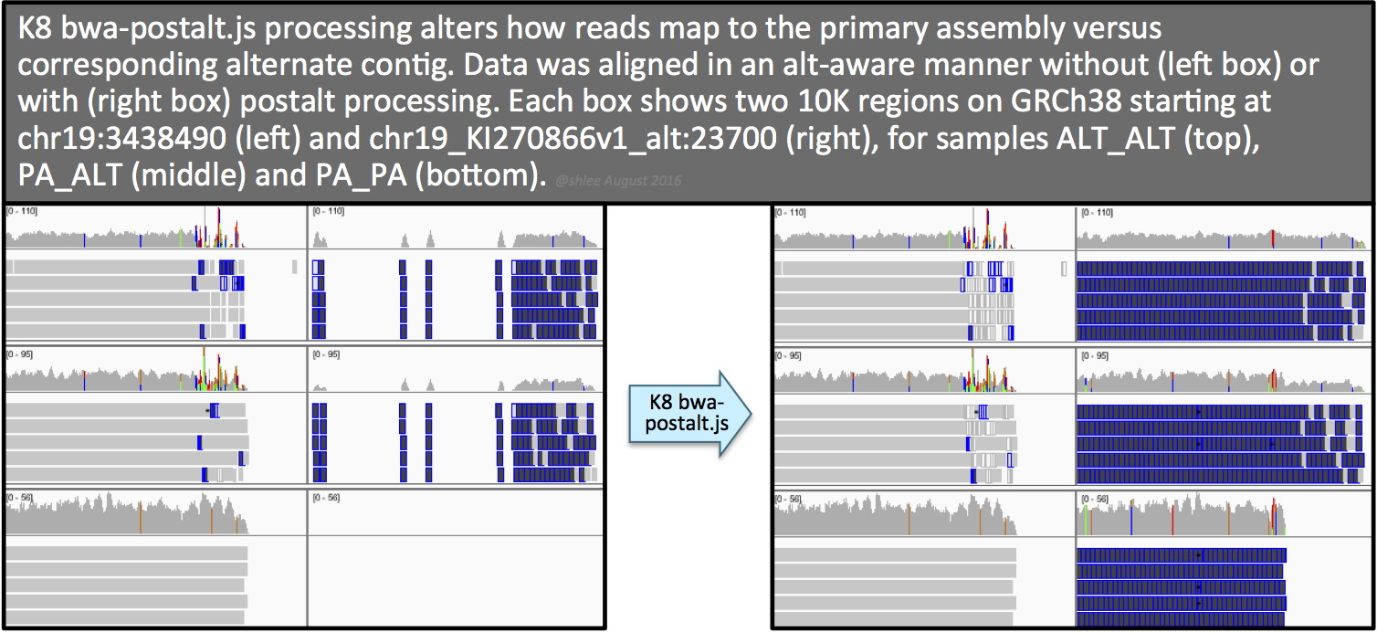](https://us.v-cdn.net/5019796/uploads/FileUpload/a5/3522324635aec94071a9ff688a4aa6.png)The resulting postalt-processed SAM, `altalt_postalt.sam`, undergoes the same processing as the first workflow (commands 4.1 through 4.7) except that (i) we omit `--max_alternate_alleles 3`and `--read_filter OverclippedRead` options for the HaplotypeCaller command like we did in **section 6.1** and (ii) we perform the 0x1 flag removal step from **section 6.1**.
137 |
138 | The effect of this postalt-processing is immediately apparent in the IGV screenshots. Previously empty regions are now filled with alignments. Look closely in the highly divergent region of the primary locus. Do you notice a change, albeit subtle, before and after postalt-processing for samples ALTALT and PAALT?
139 |
140 | These alignments give the calls below for our SNP sites of interest. Here, notice calls are made for more sites--on the equivalent site if present in addition to the design site (highlighted in the first two columns). For the three pairs of sites that can be called on either the primary locus or alternate contig, the variant site QUALs, the INFO field annotation metrics and the sample level annotation values are identical for each pair.
141 |
142 | [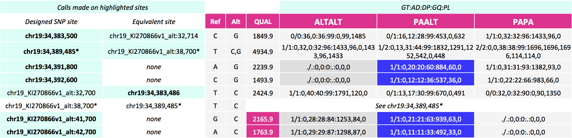](https://us.v-cdn.net/5019796/uploads/FileUpload/c4/5f07b27798374175ba40f970e77a62.png)
143 |
144 | Postalt-processing lowers the MAPQ of primary locus alignments in the highly divergent region that map better to the alt locus. You can see this as a subtle change in the IGV screenshot. After postalt-processing we see an increase in white zero MAPQ reads in the highly divergent region of the primary locus for ALTALT and PAALT. For ALTALT, this effectively cleans up the variant calls in this region at chr19:34,391,800 and chr19:34,392,600. Previously for ALTALT, these calls contained some reads: 4 and 25 for the first workflow and 0 and 28 for the second workflow. After postalt-processing, no reads are considered in this region giving us `./.:0,0:0:.:0,0,0`calls for both sites.
145 |
146 | What we omit from examination are the effects of postalt-processing on decoy contig alignments. Namely, if an alignment on the primary assembly aligns better on a decoy contig, then postalt-processing discounts the alignment on the primary assembly by assigning it a zero MAPQ score.
147 |
148 | To wrap up, here are the number of variant sites called for the three workflows. As you can see, this last workflow calls the most variants at 95 variant sites, with 62 on the primary assembly and 33 on the alternate contig.
149 |
150 | ```
151 | Workflow total on primary assembly on alternate contig
152 | tutorial_8017 56 54 2
153 | tutorial_8017_toSE 68 66 2
154 | tutorial_8017_postalt 95 62 33
155 | ```
156 |
157 | [back to top](https://software.broadinstitute.org/gatk/documentation/topic?name=tutorials#top)
158 |
159 | ------
160 |
161 | ### 7. Related resources
162 |
163 | - For WDL scripts of the workflows represented in this tutorial, see the [GATK WDL scripts repository](https://github.com/broadinstitute/wdl/tree/develop/scripts/tutorials/gatk).
164 | - To revert an aligned BAM to unaligned BAM, see **Section B** of [Tutorial#6484](https://software.broadinstitute.org/gatk/documentation/article?id=6484).
165 | - To simulate reads from a reference contig, see [Tutorial#7859](https://software.broadinstitute.org/gatk/documentation/article?id=7859).
166 | - *Dictionary* entry [Reference Genome Components](https://software.broadinstitute.org/gatk/documentation/article?id=7857) reviews terminology that describe reference genome components.
167 | - The [GATK resource bundle](https://software.broadinstitute.org/gatk/download/bundle) provides an analysis set GRCh38 reference FASTA as well as several other related resource files.
168 | - As of this writing (August 8, 2016), the SAM format ALT index file for GRCh38 is available only in the [x86_64-linux bwakit download](https://sourceforge.net/projects/bio-bwa/files/bwakit/) as stated in this [bwakit README](https://github.com/lh3/bwa/tree/master/bwakit). The `hs38DH.fa.alt` file is in the `resource-GRCh38` folder. Rename this file's basename to match that of the corresponding reference FASTA.
169 | - For more details on MergeBamAlignment features, see [Section 3C](https://software.broadinstitute.org/gatk/documentation/article?id=6483#step3C) of [Tutorial#6483](https://software.broadinstitute.org/gatk/documentation/article?id=6483).
170 | - For details on the PairedEndSingleSampleWorkflow that uses GRCh38, see [here](https://github.com/broadinstitute/wdl/blob/develop/scripts/broad_pipelines/PairedSingleSampleWf_160720.md).
171 | - See [here](https://samtools.github.io/hts-specs) for VCF specifications.
172 |
173 |
--------------------------------------------------------------------------------
/tutorials/filetype/如何对bam文件进行修复.md:
--------------------------------------------------------------------------------
1 | # 如何对bam文件进行修复
2 |
3 | 原文链接: [ (How to) Fix a badly formatted BAM](https://software.broadinstitute.org/gatk/documentation/article?id=2909)
4 |
5 | 这一个内容比较重要
6 |
7 | Fix a BAM that is not indexed or not sorted, has not had duplicates marked, or is lacking read group information. The options on this page are listed in order of decreasing complexity.
8 |
9 | You may ask, is all of this really necessary? The GATK imposes strict formatting guidelines, including requiring certain [read group information](http://gatkforums.broadinstitute.org/discussion/6472/), that other software packages do not require. Although this represents a small additional processing burden upfront, the downstream benefits are numerous, including the ability to process library data individually, and significant gains in speed and parallelization options.
10 |
11 | #### Prerequisites
12 |
13 | - Installed Picard tools
14 | - If indexing or marking duplicates, then coordinate sorted reads
15 | - If coordinate sorting, then reference aligned reads
16 | - For each read group ID, a single BAM file. If you have a multiplexed file, separate to individual files per sample.
17 |
18 | #### Jump to a section on this page
19 |
20 | 1. [Add read groups, coordinate sort and index](https://software.broadinstitute.org/gatk/documentation/topic?name=tutorials#addRG) using AddOrReplaceReadGroups
21 | 2. [Coordinate sort and index](https://software.broadinstitute.org/gatk/documentation/topic?name=tutorials#sort) using SortSam
22 | 3. [Index an already coordinate-sorted BAM](https://software.broadinstitute.org/gatk/documentation/topic?name=tutorials#index) using BuildBamIndex
23 | 4. [Mark duplicates](https://software.broadinstitute.org/gatk/documentation/topic?name=tutorials#markduplicates) using MarkDuplicates
24 |
25 | #### Tools involved
26 |
27 | - [AddOrReplaceReadGroups](http://broadinstitute.github.io/picard/command-line-overview.html#AddOrReplaceReadGroups)
28 | - [SortSam](https://broadinstitute.github.io/picard/command-line-overview.html#SortSam)
29 | - [BuildBamIndex](https://software.broadinstitute.org/gatk/documentation/broadinstitute.github.io/picard/command-line-overview.html#BuildBamIndex)
30 | - [MarkDuplicates](https://broadinstitute.github.io/picard/command-line-overview.html#MarkDuplicates)
31 |
32 | #### Related resources
33 |
34 | - Our [dictionary entry on read groups](http://gatkforums.broadinstitute.org/discussion/6472/) discusses the importance of assigning appropriate read group fields that differentiate samples and factors that contribute to batch effects, e.g. flow cell lane. Be sure that your read group fields conform to the recommendations.
35 | - [Picard's standard options](http://broadinstitute.github.io/picard/command-line-overview.html#Overview) includes adding `CREATE_INDEX` to the commands of any of its tools that produce coordinate sorted BAMs.
36 |
37 | ------
38 |
39 | ### 1. Add read groups, coordinate sort and index using AddOrReplaceReadGroups
40 |
41 | Use Picard's [AddOrReplaceReadGroups](http://broadinstitute.github.io/picard/command-line-overview.html#AddOrReplaceReadGroups) to appropriately label read group (`@RG`) fields, coordinate sort and index a BAM file. Only the five required `@RG` fields are included in the command shown. Consider the other optional `@RG` fields for better record keeping.
42 |
43 | ```
44 | java -jar picard.jar AddOrReplaceReadGroups \
45 | INPUT=reads.bam \
46 | OUTPUT=reads_addRG.bam \
47 | RGID=H0164.2 \ #be sure to change from default of 1
48 | RGLB= library1 \
49 | RGPL=illumina \
50 | RGPU=H0164ALXX140820.2 \
51 | RGSM=sample1 \
52 | ```
53 |
54 | This creates a file called `reads_addRG.bam` with the same content and sorting as the input file, except the SAM record header's `@RG` line will be updated with the new information for the specified fields and each read will now have an RG tag filled with the `@RG` ID field information. Because of this repetition, the length of the `@RG` ID field contributes to file size.
55 |
56 | To additionally coordinate sort by genomic location and create a `.bai` index, add the following options to the command.
57 |
58 | ```
59 | SORT_ORDER=coordinate \
60 | CREATE_INDEX=true
61 | ```
62 |
63 | To process large files, also designate a temporary directory.
64 |
65 | ```
66 | TMP_DIR=/path/shlee #sets environmental variable for temporary directory
67 | ```
68 |
69 | ------
70 |
71 | ### 2. Coordinate sort and index using SortSam
72 |
73 | Picard's [SortSam](https://broadinstitute.github.io/picard/command-line-overview.html#SortSam) both sorts and indexes and converts between SAM and BAM formats. For coordinate sorting, reads must be aligned to a reference genome.
74 |
75 | ```
76 | java -jar picard.jar SortSam \
77 | INPUT=reads.bam \
78 | OUTPUT=reads_sorted.bam \
79 | SORT_ORDER=coordinate \
80 | ```
81 |
82 | Concurrently index by tacking on the following option.
83 |
84 | ```
85 | CREATE_INDEX=true
86 | ```
87 |
88 | This creates a file called `reads_sorted.bam` containing reads sorted by genomic location, aka coordinate, and a `.bai` index file with the same prefix as the output, e.g. `reads_sorted.bai`, within the same directory.
89 |
90 | To process large files, also designate a temporary directory.
91 |
92 | ```
93 | TMP_DIR=/path/shlee #sets environmental variable for temporary directory
94 | ```
95 |
96 | ------
97 |
98 | ### 3. Index an already coordinate-sorted BAM using BuildBamIndex
99 |
100 | Picard's [BuildBamIndex](https://software.broadinstitute.org/gatk/documentation/broadinstitute.github.io/picard/command-line-overview.html#BuildBamIndex) allows you to index a BAM that is already coordinate sorted.
101 |
102 | ```
103 | java -jar picard.jar BuildBamIndex \
104 | INPUT=reads_sorted.bam
105 | ```
106 |
107 | This creates a `.bai` index file with the same prefix as the input file, e.g. `reads_sorted.bai`, within the same directory as the input file. You want to keep this default behavior as many tools require the same prefix and directory location for the pair of files. Note that Picard tools do not systematically create an index file when they output a new BAM file, whereas GATK tools will always output indexed files.
108 |
109 | To process large files, also designate a temporary directory.
110 |
111 | ```
112 | TMP_DIR=/path/shlee #sets environmental variable for temporary directory
113 | ```
114 |
115 | ------
116 |
117 | ### 4. Mark duplicates using MarkDuplicates
118 |
119 | Picard's [MarkDuplicates](https://broadinstitute.github.io/picard/command-line-overview.html#MarkDuplicates) flags both PCR and optical duplicate reads with a 1024 (0x400) [SAM flag](https://broadinstitute.github.io/picard/explain-flags.html). The input BAM must be coordinate sorted.
120 |
121 | ```
122 | java -jar picard.jar MarkDuplicates \
123 | INPUT=reads_sorted.bam \
124 | OUTPUT=reads_markdup.bam \
125 | METRICS_FILE=metrics.txt \
126 | CREATE_INDEX=true
127 | ```
128 |
129 | This creates a file called `reads_markdup.bam` with duplicate reads marked. It also creates a file called `metrics.txt` containing duplicate read data metrics and a `.bai` index file.
130 |
131 | To process large files, also designate a temporary directory.
132 |
133 | ```
134 | TMP_DIR=/path/shlee #sets environmental variable for temporary directory
135 | ```
136 |
137 | - During sequencing, which involves PCR amplification within the sequencing machine, by a stochastic process we end up sequencing a proportion of DNA molecules that arose from the same parent insert. To be stringent in our variant discovery, GATK tools discount the duplicate reads as evidence for or against a putative variant.
138 |
139 | - Marking duplicates is less relevant to targeted amplicon sequencing and RNA-Seq analysis.
140 |
141 | - Optical duplicates arise from a read being sequenced twice as neighboring clusters.
142 |
143 |
--------------------------------------------------------------------------------
/tutorials/filetype/如何根据坐标区间对bam文件取子集?.md:
--------------------------------------------------------------------------------
1 | # 如何根据坐标区间对bam文件取子集?
2 |
3 | 原文链接:[ (How to) Create a snippet of reads corresponding to a genomic interval](https://software.broadinstitute.org/gatk/documentation/article?id=6517)
4 |
5 |
6 |
7 | #### Tools involved
8 |
9 | - [PrintReads](https://www.broadinstitute.org/gatk/gatkdocs/org_broadinstitute_gatk_tools_walkers_readutils_PrintReads.php)
10 |
11 | #### Prerequisites
12 |
13 | - Installed GATK tools
14 | - Reference genome
15 | - Coordinate-sorted, aligned and indexed BAM
16 |
17 | #### Download example data
18 |
19 | - Use the [advanced tutorial bundle](http://gatkforums.broadinstitute.org/discussion/4610/)'s human_g1k_v37_decoy.fasta as reference
20 | - [tutorial_6517.tar.gz](https://drive.google.com/open?id=0BzI1CyccGsZiTmlDLW13MXdTSG8) contains four files: 6517_2Mbp_input.bam and .bai covering reads aligning to 10:90,000,000-92,000,000 and 6517_1Mbp_output.bam and .bai covering 10:91,000,000-92,000,000
21 |
22 | #### Related resources
23 |
24 | - This *How to* is referenced in a tutorial on [(How to) Generate an unmapped BAM (uBAM)](http://gatkforums.broadinstitute.org/discussion/6484/).
25 | - See [this tutorial](http://gatkforums.broadinstitute.org/discussion/2909/) to coordinate-sort and index a BAM.
26 | - See [here](https://www.broadinstitute.org/gatk/gatkdocs/org_broadinstitute_gatk_engine_CommandLineGATK.php#--unsafe) for command line parameters accepted by all GATK tools.
27 | - For applying interval lists, e.g. to whole exome data, see [When should I use L to pass in a list of intervals](http://gatkforums.broadinstitute.org/discussion/4133/when-should-i-use-l-to-pass-in-a-list-of-intervals).
28 |
29 | ------
30 |
31 | ### Create a snippet of reads corresponding to a genomic interval using PrintReads
32 |
33 | PrintReads merges or subsets sequence data. The tool automatically applies MalformedReadFilter and BadCigarFilter to filter out certain types of reads that cause problems for downstream GATK tools, e.g. reads with mismatching numbers of bases and base qualities or reads with CIGAR strings containing the N operator.
34 |
35 | - To create a test snippet of RNA-Seq data that retains reads with Ns in CIGAR strings, use `-U ALLOW_N_CIGAR_READS`.
36 |
37 | Subsetting reads corresponding to a genomic interval using PrintReads requires reads that are aligned to a reference genome, coordinate-sorted and indexed. Place the `.bai` index in the same directory as the `.bam` file.
38 |
39 | ```
40 | java -Xmx8G -jar /path/GenomeAnalysisTK.jar \
41 | -T PrintReads \
42 | -R /path/human_g1k_v37_decoy.fasta \ #reference fasta
43 | -L 10:91000000-92000000 \ #desired genomic interval chr:start-end
44 | -I 6517_2Mbp_input.bam \ #input
45 | -o 6517_1Mbp_output.bam
46 | ```
47 |
48 | This creates a subset of reads from the input file, `6517_2Mbp_input.bam`, that align to the interval defined by the `-L` option, here a 1 Mbp region on chromosome 10. The tool creates two new files, `6517_1Mbp_output.bam`and corresponding index `6517_1Mbp_output.bai`.
49 |
50 | - For paired reads, the tool does not account for reads whose mate aligns outside of the defined interval. To filter these lost mate reads, use RevertSam's `SANITIZE` option.
51 |
52 | To process large files, also designate a temporary directory.
53 |
54 | ```
55 | TMP_DIR=/path/shlee #sets environmental variable for temporary directory
56 | ```
--------------------------------------------------------------------------------
/tutorials/steps/如何用HC找变异.md:
--------------------------------------------------------------------------------
1 | # 如何用HC找变异
2 |
3 | 原文链接:[ (howto) Call variants with HaplotypeCaller](https://software.broadinstitute.org/gatk/documentation/article?id=2803)
4 |
5 | 这个内容比较单一,就是翻译一个命令的使用
6 |
7 | #### Objective
8 |
9 | Call variants on a single genome with the HaplotypeCaller, producing a raw (unfiltered) VCF.
10 |
11 | #### Caveat
12 |
13 | This is meant only for single-sample analysis. To analyze multiple samples, see the Best Practices documentation on joint analysis.
14 |
15 | #### Prerequisites
16 |
17 | - TBD
18 |
19 | #### Steps
20 |
21 | 1. Determine the basic parameters of the analysis
22 | 2. Call variants in your sequence data
23 |
24 | ------
25 |
26 | ### 1. Determine the basic parameters of the analysis
27 |
28 | If you do not specify these parameters yourself, the program will use default values. However we recommend that you set them explicitly because it will help you understand how the results are bounded and how you can modify the program's behavior.
29 |
30 | - Genotyping mode (`--genotyping_mode`)
31 |
32 | This specifies how we want the program to determine the alternate alleles to use for genotyping. In the default `DISCOVERY` mode, the program will choose the most likely alleles out of those it sees in the data. In `GENOTYPE_GIVEN_ALLELES` mode, the program will only use the alleles passed in from a VCF file (using the `-alleles` argument). This is useful if you just want to determine if a sample has a specific genotype of interest and you are not interested in other alleles.
33 |
34 | - Emission confidence threshold (`-stand_emit_conf`)
35 |
36 | This is the minimum confidence threshold (phred-scaled) at which the program should emit sites that appear to be possibly variant.
37 |
38 | - Calling confidence threshold (`-stand_call_conf`)
39 |
40 | This is the minimum confidence threshold (phred-scaled) at which the program should emit variant sites as called. If a site's associated genotype has a confidence score lower than the calling threshold, the program will emit the site as filtered and will annotate it as LowQual. This threshold separates high confidence calls from low confidence calls.
41 |
42 | *The terms "called" and "filtered" are tricky because they can mean different things depending on context. In ordinary language, people often say a site was called if it was emitted as variant. But in the GATK's technical language, saying a site was called means that that site passed the confidence threshold test. For filtered, it's even more confusing, because in ordinary language, when people say that sites were filtered, they usually mean that those sites successfully passed a filtering test. However, in the GATK's technical language, the same phrase (saying that sites were filtered) means that those sites failed the filtering test. In effect, it means that those would be filtered out if the filter was used to actually remove low-confidence calls from the callset, instead of just tagging them. In both cases, both usages are valid depending on the point of view of the person who is reporting the results. So it's always important to check what is the context when interpreting results that include these terms.*
43 |
44 | ------
45 |
46 | ### 2. Call variants in your sequence data
47 |
48 | #### Action
49 |
50 | Run the following GATK command:
51 |
52 | ```
53 | java -jar GenomeAnalysisTK.jar \
54 | -T HaplotypeCaller \
55 | -R reference.fa \
56 | -I preprocessed_reads.bam \
57 | -L 20 \
58 | --genotyping_mode DISCOVERY \
59 | -stand_emit_conf 10 \
60 | -stand_call_conf 30 \
61 | -o raw_variants.vcf
62 | ```
63 |
64 | *Note that -L specifies that we only want to run the command on a subset of the data (here, chromosome 20). This is useful for testing as well as other purposes, as documented here. For example, when running on exome data, we use -L to specify a file containing the list of exome targets corresponding to the capture kit that was used to generate the exome libraries.*
65 |
66 | #### Expected Result
67 |
68 | This creates a VCF file called `raw_variants.vcf`, containing all the sites that the HaplotypeCaller evaluated to be potentially variant. Note that this file contains both SNPs and Indels.
69 |
70 | Although you now have a nice fresh set of variant calls, the variant discovery stage is not over. The distinctions made by the caller itself between low-confidence calls and the rest is very primitive, and should not be taken as a definitive guide for filtering. The GATK callers are designed to be very lenient in calling variants, so it is extremely important to apply one of the recommended filtering methods (variant recalibration or hard-filtering), in order to move on to downstream analyses with the highest-quality call set possible.
71 |
72 |
73 |
74 |
--------------------------------------------------------------------------------
/tutorials/steps/如何用UG找变异.md:
--------------------------------------------------------------------------------
1 | # 如何用UG找变异
2 |
3 | 原文链接: [ (howto) Call variants with the UnifiedGenotyper](https://software.broadinstitute.org/gatk/documentation/article?id=2804)
4 |
5 | 这个内容比较单一,就是翻译一个命令的使用,但是GATK官方推荐不用这个工具了。
6 |
7 | 所以不需要翻译。
8 |
9 |
--------------------------------------------------------------------------------
/tutorials/steps/如何运行BQSR.md:
--------------------------------------------------------------------------------
1 | # 如何运行BQSR
2 |
3 | 原文链接: [ (howto) Recalibrate base quality scores = run BQSR](https://software.broadinstitute.org/gatk/documentation/article?id=2801)
4 |
5 | 内容不多,需要翻译
6 |
7 | #### Objective
8 |
9 | Recalibrate base quality scores in order to correct sequencing errors and other experimental artifacts.
10 |
11 | #### Prerequisites
12 |
13 | - TBD
14 |
15 | #### Steps
16 |
17 | 1. Analyze patterns of covariation in the sequence dataset
18 | 2. Do a second pass to analyze covariation remaining after recalibration
19 | 3. Generate before/after plots
20 | 4. Apply the recalibration to your sequence data
21 |
22 | ------
23 |
24 | ### 1. Analyze patterns of covariation in the sequence dataset
25 |
26 | #### Action
27 |
28 | Run the following GATK command:
29 |
30 | ```
31 | java -jar GenomeAnalysisTK.jar \
32 | -T BaseRecalibrator \
33 | -R reference.fa \
34 | -I input_reads.bam \
35 | -L 20 \
36 | -knownSites dbsnp.vcf \
37 | -knownSites gold_indels.vcf \
38 | -o recal_data.table
39 | ```
40 |
41 | #### Expected Result
42 |
43 | This creates a GATKReport file called `recal_data.table` containing several tables. These tables contain the covariation data that will be used in a later step to recalibrate the base qualities of your sequence data.
44 |
45 | It is imperative that you provide the program with a set of known sites, otherwise it will refuse to run. The known sites are used to build the covariation model and estimate empirical base qualities. For details on what to do if there are no known sites available for your organism of study, please see the online GATK documentation.
46 |
47 | Note that `-L 20` is used here and in the next steps to restrict analysis to only chromosome 20 in the b37 human genome reference build. To run against a different reference, you may need to change the name of the contig according to the nomenclature used in your reference.
48 |
49 | ------
50 |
51 | ### 2. Do a second pass to analyze covariation remaining after recalibration
52 |
53 | #### Action
54 |
55 | Run the following GATK command:
56 |
57 | ```
58 | java -jar GenomeAnalysisTK.jar \
59 | -T BaseRecalibrator \
60 | -R reference.fa \
61 | -I input_reads.bam \
62 | -L 20 \
63 | -knownSites dbsnp.vcf \
64 | -knownSites gold_indels.vcf \
65 | -BQSR recal_data.table \
66 | -o post_recal_data.table
67 | ```
68 |
69 | #### Expected Result
70 |
71 | This creates another GATKReport file, which we will use in the next step to generate plots. Note the use of the `-BQSR` flag, which tells the GATK engine to perform on-the-fly recalibration based on the first recalibration data table.
72 |
73 | ------
74 |
75 | ### 3. Generate before/after plots
76 |
77 | #### Action
78 |
79 | Run the following GATK command:
80 |
81 | ```
82 | java -jar GenomeAnalysisTK.jar \
83 | -T AnalyzeCovariates \
84 | -R reference.fa \
85 | -L 20 \
86 | -before recal_data.table \
87 | -after post_recal_data.table \
88 | -plots recalibration_plots.pdf
89 | ```
90 |
91 | #### Expected Result
92 |
93 | This generates a document called `recalibration_plots.pdf` containing plots that show how the reported base qualities match up to the empirical qualities calculated by the BaseRecalibrator. Comparing the **before** and **after**plots allows you to check the effect of the base recalibration process before you actually apply the recalibration to your sequence data. For details on how to interpret the base recalibration plots, please see the online GATK documentation.
94 |
95 | ------
96 |
97 | ### 4. Apply the recalibration to your sequence data
98 |
99 | #### Action
100 |
101 | Run the following GATK command:
102 |
103 | ```
104 | java -jar GenomeAnalysisTK.jar \
105 | -T PrintReads \
106 | -R reference.fa \
107 | -I input_reads.bam \
108 | -L 20 \
109 | -BQSR recal_data.table \
110 | -o recal_reads.bam
111 | ```
112 |
113 | #### Expected Result
114 |
115 | This creates a file called `recal_reads.bam` containing all the original reads, but now with exquisitely accurate base substitution, insertion and deletion quality scores. By default, the original quality scores are discarded in order to keep the file size down. However, you have the option to retain them by adding the flag `–emit_original_quals` to the PrintReads command, in which case the original qualities will also be written in the file, tagged `OQ`.
116 |
117 | Notice how this step uses a very simple tool, PrintReads, to apply the recalibration. What’s happening here is that we are loading in the original sequence data, having the GATK engine recalibrate the base qualities on-the-fly thanks to the `-BQSR` flag (as explained earlier), and just using PrintReads to write out the resulting data to the new file.
--------------------------------------------------------------------------------
/tutorials/steps/如何运行VQSR.md:
--------------------------------------------------------------------------------
1 | # 如何运行VQSR
2 |
3 | 原文链接: [ (howto) Recalibrate variant quality scores = run VQSR](https://software.broadinstitute.org/gatk/documentation/article?id=2805)
4 |
5 | 内容有点多,估计跟GATK最佳实践也是很大部分重合着的
6 |
7 | #### Objective
8 |
9 | Recalibrate variant quality scores and produce a callset filtered for the desired levels of sensitivity and specificity.
10 |
11 | #### Prerequisites
12 |
13 | - TBD
14 |
15 | #### Caveats
16 |
17 | This document provides a typical usage example including parameter values. However, the values given may not be representative of the latest Best Practices recommendations. When in doubt, please consult the [FAQ document on VQSR training sets and parameters](https://www.broadinstitute.org/gatk/guide/article?id=1259), which overrides this document. See that document also for caveats regarding exome vs. whole genomes analysis design.
18 |
19 | #### Steps
20 |
21 | 1. Prepare recalibration parameters for SNPs
22 | a. Specify which call sets the program should use as resources to build the recalibration model
23 | b. Specify which annotations the program should use to evaluate the likelihood of Indels being real
24 | c. Specify the desired truth sensitivity threshold values that the program should use to generate tranches
25 | d. Determine additional model parameters
26 | 2. Build the SNP recalibration model
27 | 3. Apply the desired level of recalibration to the SNPs in the call set
28 | 4. Prepare recalibration parameters for Indels a. Specify which call sets the program should use as resources to build the recalibration model b. Specify which annotations the program should use to evaluate the likelihood of Indels being real c. Specify the desired truth sensitivity threshold values that the program should use to generate tranches d. Determine additional model parameters
29 | 5. Build the Indel recalibration model
30 | 6. Apply the desired level of recalibration to the Indels in the call set
31 |
32 | ------
33 |
34 | ### 1. Prepare recalibration parameters for SNPs
35 |
36 | #### a. Specify which call sets the program should use as resources to build the recalibration model
37 |
38 | For each training set, we use key-value tags to qualify whether the set contains known sites, training sites, and/or truth sites. We also use a tag to specify the prior likelihood that those sites are true (using the Phred scale).
39 |
40 | - True sites training resource: HapMap
41 |
42 | This resource is a SNP call set that has been validated to a very high degree of confidence. The program will consider that the variants in this resource are representative of true sites (truth=true), and will use them to train the recalibration model (training=true). We will also use these sites later on to choose a threshold for filtering variants based on sensitivity to truth sites. The prior likelihood we assign to these variants is Q15 (96.84%).
43 |
44 | - True sites training resource: Omni
45 |
46 | This resource is a set of polymorphic SNP sites produced by the Omni genotyping array. The program will consider that the variants in this resource are representative of true sites (truth=true), and will use them to train the recalibration model (training=true). The prior likelihood we assign to these variants is Q12 (93.69%).
47 |
48 | - Non-true sites training resource: 1000G
49 |
50 | This resource is a set of high-confidence SNP sites produced by the 1000 Genomes Project. The program will consider that the variants in this resource may contain true variants as well as false positives (truth=false), and will use them to train the recalibration model (training=true). The prior likelihood we assign to these variants is Q10 (90%).
51 |
52 | - Known sites resource, not used in training: dbSNP
53 |
54 | This resource is a SNP call set that has not been validated to a high degree of confidence (truth=false). The program will not use the variants in this resource to train the recalibration model (training=false). However, the program will use these to stratify output metrics such as Ti/Tv ratio by whether variants are present in dbsnp or not (known=true). The prior likelihood we assign to these variants is Q2 (36.90%).
55 |
56 | *The default prior likelihood assigned to all other variants is Q2 (36.90%). This low value reflects the fact that the philosophy of the GATK callers is to produce a large, highly sensitive callset that needs to be heavily refined through additional filtering.*
57 |
58 | #### b. Specify which annotations the program should use to evaluate the likelihood of SNPs being real
59 |
60 | These annotations are included in the information generated for each variant call by the caller. If an annotation is missing (typically because it was omitted from the calling command) it can be added using the VariantAnnotator tool.
61 |
62 | - [Coverage (DP)](https://www.broadinstitute.org/gatk/guide/tooldocs/org_broadinstitute_gatk_tools_walkers_annotator_Coverage.php)
63 |
64 | Total (unfiltered) depth of coverage. Note that this statistic should not be used with exome datasets; see caveat detailed in the [VQSR arguments FAQ doc](https://software.broadinstitute.org/gatk/documentation/(https://www.broadinstitute.org/gatk/guide/article?id=1259)).
65 |
66 | - [QualByDepth (QD)](https://www.broadinstitute.org/gatk/guide/tooldocs/org_broadinstitute_gatk_tools_walkers_annotator_QualByDepth.php)
67 |
68 | Variant confidence (from the QUAL field) / unfiltered depth of non-reference samples.
69 |
70 | - [FisherStrand (FS)](https://www.broadinstitute.org/gatk/guide/tooldocs/org_broadinstitute_gatk_tools_walkers_annotator_StrandOddsRatio.php)
71 |
72 | Measure of strand bias (the variation being seen on only the forward or only the reverse strand). More bias is indicative of false positive calls. This complements the [StrandOddsRatio (SOR)](https://www.broadinstitute.org/gatk/guide/tooldocs/org_broadinstitute_gatk_tools_walkers_annotator_StrandOddsRatio.php) annotation.
73 |
74 | - [StrandOddsRatio (SOR)](https://www.broadinstitute.org/gatk/guide/tooldocs/org_broadinstitute_gatk_tools_walkers_annotator_StrandOddsRatio.php)
75 |
76 | Measure of strand bias (the variation being seen on only the forward or only the reverse strand). More bias is indicative of false positive calls. This complements the [FisherStrand (FS)](https://www.broadinstitute.org/gatk/guide/tooldocs/org_broadinstitute_gatk_tools_walkers_annotator_FisherStrand.php) annotation.
77 |
78 | - [MappingQualityRankSumTest (MQRankSum)](https://www.broadinstitute.org/gatk/guide/tooldocs/org_broadinstitute_gatk_tools_walkers_annotator_MappingQualityRankSumTest.php)
79 |
80 | The rank sum test for mapping qualities. Note that the mapping quality rank sum test can not be calculated for sites without a mixture of reads showing both the reference and alternate alleles.
81 |
82 | - [ReadPosRankSumTest (ReadPosRankSum)](https://www.broadinstitute.org/gatk/guide/tooldocs/org_broadinstitute_gatk_tools_walkers_annotator_ReadPosRankSumTest.php)
83 |
84 | The rank sum test for the distance from the end of the reads. If the alternate allele is only seen near the ends of reads, this is indicative of error. Note that the read position rank sum test can not be calculated for sites without a mixture of reads showing both the reference and alternate alleles.
85 |
86 | - [RMSMappingQuality (MQ)](https://www.broadinstitute.org/gatk/guide/tooldocs/org_broadinstitute_gatk_tools_walkers_annotator_RMSMappingQuality.php)
87 |
88 | Estimation of the overall mapping quality of reads supporting a variant call.
89 |
90 | - [InbreedingCoeff](https://www.broadinstitute.org/gatk/guide/tooldocs/org_broadinstitute_gatk_tools_walkers_annotator_InbreedingCoeff.php)
91 |
92 | Evidence of inbreeding in a population. See caveats regarding population size and composition detailed in the [VQSR arguments FAQ doc](https://software.broadinstitute.org/gatk/documentation/(https://www.broadinstitute.org/gatk/guide/article?id=1259)).
93 |
94 | #### c. Specify the desired truth sensitivity threshold values that the program should use to generate tranches
95 |
96 | - First tranche threshold 100.0
97 | - Second tranche threshold 99.9
98 | - Third tranche threshold 99.0
99 | - Fourth tranche threshold 90.0
100 |
101 | Tranches are essentially slices of variants, ranked by VQSLOD, bounded by the threshold values specified in this step. The threshold values themselves refer to the sensitivity we can obtain when we apply them to the call sets that the program uses to train the model. The idea is that the lowest tranche is highly specific but less sensitive (there are very few false positives but potentially many false negatives, i.e. missing calls), and each subsequent tranche in turn introduces additional true positive calls along with a growing number of false positive calls. This allows us to filter variants based on how sensitive we want the call set to be, rather than applying hard filters and then only evaluating how sensitive the call set is using post hoc methods.
102 |
103 | ------
104 |
105 | ### 2. Build the SNP recalibration model
106 |
107 | #### Action
108 |
109 | Run the following GATK command:
110 |
111 | ```
112 | java -jar GenomeAnalysisTK.jar \
113 | -T VariantRecalibrator \
114 | -R reference.fa \
115 | -input raw_variants.vcf \
116 | -resource:hapmap,known=false,training=true,truth=true,prior=15.0 hapmap.vcf \
117 | -resource:omni,known=false,training=true,truth=true,prior=12.0 omni.vcf \
118 | -resource:1000G,known=false,training=true,truth=false,prior=10.0 1000G.vcf \
119 | -resource:dbsnp,known=true,training=false,truth=false,prior=2.0 dbsnp.vcf \
120 | -an DP \
121 | -an QD \
122 | -an FS \
123 | -an SOR \
124 | -an MQ \
125 | -an MQRankSum \
126 | -an ReadPosRankSum \
127 | -an InbreedingCoeff \
128 | -mode SNP \
129 | -tranche 100.0 -tranche 99.9 -tranche 99.0 -tranche 90.0 \
130 | -recalFile recalibrate_SNP.recal \
131 | -tranchesFile recalibrate_SNP.tranches \
132 | -rscriptFile recalibrate_SNP_plots.R
133 | ```
134 |
135 | #### Expected Result
136 |
137 | This creates several files. The most important file is the recalibration report, called `recalibrate_SNP.recal`, which contains the recalibration data. This is what the program will use in the next step to generate a VCF file in which the variants are annotated with their recalibrated quality scores. There is also a file called `recalibrate_SNP.tranches`, which contains the quality score thresholds corresponding to the tranches specified in the original command. Finally, if your installation of R and the other required libraries was done correctly, you will also find some PDF files containing plots. These plots illustrated the distribution of variants according to certain dimensions of the model.
138 |
139 | For detailed instructions on how to interpret these plots, please refer to the [VQSR method documentation](https://www.broadinstitute.org/gatk/guide/article?id=39) and [presentation videos](https://www.broadinstitute.org/gatk/guide/presentations).
140 |
141 | ------
142 |
143 | ### 3. Apply the desired level of recalibration to the SNPs in the call set
144 |
145 | #### Action
146 |
147 | Run the following GATK command:
148 |
149 | ```
150 | java -jar GenomeAnalysisTK.jar \
151 | -T ApplyRecalibration \
152 | -R reference.fa \
153 | -input raw_variants.vcf \
154 | -mode SNP \
155 | --ts_filter_level 99.0 \
156 | -recalFile recalibrate_SNP.recal \
157 | -tranchesFile recalibrate_SNP.tranches \
158 | -o recalibrated_snps_raw_indels.vcf
159 | ```
160 |
161 | #### Expected Result
162 |
163 | This creates a new VCF file, called `recalibrated_snps_raw_indels.vcf`, which contains all the original variants from the original `raw_variants.vcf` file, but now the SNPs are annotated with their recalibrated quality scores (VQSLOD) and either `PASS` or `FILTER` depending on whether or not they are included in the selected tranche.
164 |
165 | Here we are taking the second lowest of the tranches specified in the original recalibration command. This means that we are applying to our data set the level of sensitivity that would allow us to retrieve 99% of true variants from the truth training sets of HapMap and Omni SNPs. If we wanted to be more specific (and therefore have less risk of including false positives, at the risk of missing real sites) we could take the very lowest tranche, which would only retrieve 90% of the truth training sites. If we wanted to be more sensitive (and therefore less specific, at the risk of including more false positives) we could take the higher tranches. In our Best Practices documentation, we recommend taking the second highest tranche (99.9%) which provides the highest sensitivity you can get while still being acceptably specific.
166 |
167 | ------
168 |
169 | ### 4. Prepare recalibration parameters for Indels
170 |
171 | #### a. Specify which call sets the program should use as resources to build the recalibration model
172 |
173 | For each training set, we use key-value tags to qualify whether the set contains known sites, training sites, and/or truth sites. We also use a tag to specify the prior likelihood that those sites are true (using the Phred scale).
174 |
175 | - Known and true sites training resource: Mills
176 |
177 | This resource is an Indel call set that has been validated to a high degree of confidence. The program will consider that the variants in this resource are representative of true sites (truth=true), and will use them to train the recalibration model (training=true). The prior likelihood we assign to these variants is Q12 (93.69%).
178 |
179 | The default prior likelihood assigned to all other variants is Q2 (36.90%). This low value reflects the fact that the philosophy of the GATK callers is to produce a large, highly sensitive callset that needs to be heavily refined through additional filtering.
180 |
181 | #### b. Specify which annotations the program should use to evaluate the likelihood of Indels being real
182 |
183 | These annotations are included in the information generated for each variant call by the caller. If an annotation is missing (typically because it was omitted from the calling command) it can be added using the VariantAnnotator tool.
184 |
185 | - [Coverage (DP)](https://www.broadinstitute.org/gatk/guide/tooldocs/org_broadinstitute_gatk_tools_walkers_annotator_Coverage.php)
186 |
187 | Total (unfiltered) depth of coverage. Note that this statistic should not be used with exome datasets; see caveat detailed in the [VQSR arguments FAQ doc](https://software.broadinstitute.org/gatk/documentation/(https://www.broadinstitute.org/gatk/guide/article?id=1259)).
188 |
189 | - [QualByDepth (QD)](https://www.broadinstitute.org/gatk/guide/tooldocs/org_broadinstitute_gatk_tools_walkers_annotator_QualByDepth.php)
190 |
191 | Variant confidence (from the QUAL field) / unfiltered depth of non-reference samples.
192 |
193 | - [FisherStrand (FS)](https://www.broadinstitute.org/gatk/guide/tooldocs/org_broadinstitute_gatk_tools_walkers_annotator_StrandOddsRatio.php)
194 |
195 | Measure of strand bias (the variation being seen on only the forward or only the reverse strand). More bias is indicative of false positive calls. This complements the [StrandOddsRatio (SOR)](https://www.broadinstitute.org/gatk/guide/tooldocs/org_broadinstitute_gatk_tools_walkers_annotator_StrandOddsRatio.php) annotation.
196 |
197 | - [StrandOddsRatio (SOR)](https://www.broadinstitute.org/gatk/guide/tooldocs/org_broadinstitute_gatk_tools_walkers_annotator_StrandOddsRatio.php)
198 |
199 | Measure of strand bias (the variation being seen on only the forward or only the reverse strand). More bias is indicative of false positive calls. This complements the [FisherStrand (FS)](https://www.broadinstitute.org/gatk/guide/tooldocs/org_broadinstitute_gatk_tools_walkers_annotator_FisherStrand.php) annotation.
200 |
201 | - [MappingQualityRankSumTest (MQRankSum)](https://www.broadinstitute.org/gatk/guide/tooldocs/org_broadinstitute_gatk_tools_walkers_annotator_MappingQualityRankSumTest.php)
202 |
203 | The rank sum test for mapping qualities. Note that the mapping quality rank sum test can not be calculated for sites without a mixture of reads showing both the reference and alternate alleles.
204 |
205 | - [ReadPosRankSumTest (ReadPosRankSum)](https://www.broadinstitute.org/gatk/guide/tooldocs/org_broadinstitute_gatk_tools_walkers_annotator_ReadPosRankSumTest.php)
206 |
207 | The rank sum test for the distance from the end of the reads. If the alternate allele is only seen near the ends of reads, this is indicative of error. Note that the read position rank sum test can not be calculated for sites without a mixture of reads showing both the reference and alternate alleles.
208 |
209 | - [InbreedingCoeff](https://www.broadinstitute.org/gatk/guide/tooldocs/org_broadinstitute_gatk_tools_walkers_annotator_InbreedingCoeff.php)
210 |
211 | Evidence of inbreeding in a population. See caveats regarding population size and composition detailed in the [VQSR arguments FAQ doc](https://software.broadinstitute.org/gatk/documentation/(https://www.broadinstitute.org/gatk/guide/article?id=1259)).
212 |
213 | #### c. Specify the desired truth sensitivity threshold values that the program should use to generate tranches
214 |
215 | - First tranche threshold 100.0
216 | - Second tranche threshold 99.9
217 | - Third tranche threshold 99.0
218 | - Fourth tranche threshold 90.0
219 |
220 | Tranches are essentially slices of variants, ranked by VQSLOD, bounded by the threshold values specified in this step. The threshold values themselves refer to the sensitivity we can obtain when we apply them to the call sets that the program uses to train the model. The idea is that the lowest tranche is highly specific but less sensitive (there are very few false positives but potentially many false negatives, i.e. missing calls), and each subsequent tranche in turn introduces additional true positive calls along with a growing number of false positive calls. This allows us to filter variants based on how sensitive we want the call set to be, rather than applying hard filters and then only evaluating how sensitive the call set is using post hoc methods.
221 |
222 | #### d. Determine additional model parameters
223 |
224 | - Maximum number of Gaussians (`-maxGaussians`) 4
225 |
226 | This is the maximum number of Gaussians (*i.e.* clusters of variants that have similar properties) that the program should try to identify when it runs the variational Bayes algorithm that underlies the machine learning method. In essence, this limits the number of different ”profiles” of variants that the program will try to identify. This number should only be increased for datasets that include very many variants.
227 |
228 | ------
229 |
230 | ### 5. Build the Indel recalibration model
231 |
232 | #### Action
233 |
234 | Run the following GATK command:
235 |
236 | ```
237 | java -jar GenomeAnalysisTK.jar \
238 | -T VariantRecalibrator \
239 | -R reference.fa \
240 | -input recalibrated_snps_raw_indels.vcf \
241 | -resource:mills,known=false,training=true,truth=true,prior=12.0 Mills_and_1000G_gold_standard.indels.b37.sites.vcf \
242 | -resource:dbsnp,known=true,training=false,truth=false,prior=2.0 dbsnp.b37.vcf \
243 | -an QD \
244 | -an DP \
245 | -an FS \
246 | -an SOR \
247 | -an MQRankSum \
248 | -an ReadPosRankSum \
249 | -an InbreedingCoeff
250 | -mode INDEL \
251 | -tranche 100.0 -tranche 99.9 -tranche 99.0 -tranche 90.0 \
252 | --maxGaussians 4 \
253 | -recalFile recalibrate_INDEL.recal \
254 | -tranchesFile recalibrate_INDEL.tranches \
255 | -rscriptFile recalibrate_INDEL_plots.R
256 | ```
257 |
258 | #### Expected Result
259 |
260 | This creates several files. The most important file is the recalibration report, called `recalibrate_INDEL.recal`, which contains the recalibration data. This is what the program will use in the next step to generate a VCF file in which the variants are annotated with their recalibrated quality scores. There is also a file called `recalibrate_INDEL.tranches`, which contains the quality score thresholds corresponding to the tranches specified in the original command. Finally, if your installation of R and the other required libraries was done correctly, you will also find some PDF files containing plots. These plots illustrated the distribution of variants according to certain dimensions of the model.
261 |
262 | For detailed instructions on how to interpret these plots, please refer to the online GATK documentation.
263 |
264 | ------
265 |
266 | ### 6. Apply the desired level of recalibration to the Indels in the call set
267 |
268 | #### Action
269 |
270 | Run the following GATK command:
271 |
272 | ```
273 | java -jar GenomeAnalysisTK.jar \
274 | -T ApplyRecalibration \
275 | -R reference.fa \
276 | -input recalibrated_snps_raw_indels.vcf \
277 | -mode INDEL \
278 | --ts_filter_level 99.0 \
279 | -recalFile recalibrate_INDEL.recal \
280 | -tranchesFile recalibrate_INDEL.tranches \
281 | -o recalibrated_variants.vcf
282 | ```
283 |
284 | #### Expected Result
285 |
286 | This creates a new VCF file, called `recalibrated_variants.vcf`, which contains all the original variants from the original `recalibrated_snps_raw_indels.vcf` file, but now the Indels are also annotated with their recalibrated quality scores (VQSLOD) and either `PASS` or `FILTER` depending on whether or not they are included in the selected tranche.
287 |
288 | Here we are taking the second lowest of the tranches specified in the original recalibration command. This means that we are applying to our data set the level of sensitivity that would allow us to retrieve 99% of true variants from the truth training sets of HapMap and Omni SNPs. If we wanted to be more specific (and therefore have less risk of including false positives, at the risk of missing real sites) we could take the very lowest tranche, which would only retrieve 90% of the truth training sites. If we wanted to be more sensitive (and therefore less specific, at the risk of including more false positives) we could take the higher tranches. In our Best Practices documentation, we recommend taking the second highest tranche (99.9%) which provides the highest sensitivity you can get while still being acceptably specific.
--------------------------------------------------------------------------------
/tutorials/vcf-filter-annotation/.DS_Store:
--------------------------------------------------------------------------------
https://raw.githubusercontent.com/gatk-chinese/forum/01188653096fa32c9a32de3e19f8423cddede238/tutorials/vcf-filter-annotation/.DS_Store
--------------------------------------------------------------------------------
/tutorials/vcf-filter-annotation/GVCF和普通的VCF文件的区别是什么.md:
--------------------------------------------------------------------------------
1 | # GVCF和普通的VCF文件的区别是什么?
2 |
3 | 原文链接:[ What is a GVCF and how is it different from a 'regular' VCF? ](https://software.broadinstitute.org/gatk/documentation/article?id=4017)
4 |
5 |
6 |
7 | ### Overview
8 |
9 | GVCF stands for Genomic VCF. A GVCF is a kind of VCF, so the basic format specification is the same as for a regular VCF (see the spec documentation [here](http://vcftools.sourceforge.net/specs.html)), but a Genomic VCF contains extra information.
10 |
11 | This document explains what that extra information is and how you can use it to empower your variants analyses.
12 |
13 | ### Important caveat
14 |
15 | What we're covering here is strictly limited to GVCFs produced by HaplotypeCaller in GATK versions 3.0 and above. The term GVCF is sometimes used simply to describe VCFs that contain a record for every position in the genome (or interval of interest) regardless of whether a variant was detected at that site or not (such as VCFs produced by UnifiedGenotyper with `--output_mode EMIT_ALL_SITES`). GVCFs produced by HaplotypeCaller 3.x contain additional information that is formatted in a very specific way. Read on to find out more.
16 |
17 | ### General comparison of VCF vs. gVCF
18 |
19 | The key difference between a regular VCF and a gVCF is that the gVCF has records for all sites, whether there is a variant call there or not. The goal is to have every site represented in the file in order to do [joint analysis of a cohort](http://www.broadinstitute.org/gatk/guide/article?id=3893) in subsequent steps. The records in a gVCF include an accurate estimation of how confident we are in the determination that the sites are homozygous-reference or not. This estimation is generated by the HaplotypeCaller's built-in [reference model](http://www.broadinstitute.org/gatk/guide/article?id=4042).
20 |
21 | 
22 |
23 | Note that some other tools (including the GATK's own UnifiedGenotyper) may output an all-sites VCF that looks superficially like the `BP_RESOLUTION` gVCFs produced by HaplotypeCaller, but they do not provide an accurate estimate of reference confidence, and therefore cannot be used in joint genotyping analyses.
24 |
25 | ### The two types of gVCFs
26 |
27 | As you can see in the figure above, there are two options you can use with `-ERC`: `GVCF` and `BP_RESOLUTION`. With `BP_RESOLUTION`, you get a gVCF with an individual record at every site: either a variant record, or a non-variant record. With `GVCF`, you get a gVCF with individual variant records for variant sites, but the non-variant sites are grouped together into non-variant block records that represent intervals of sites for which the genotype quality (GQ) is within a certain range or band. The GQ ranges are defined in the `##GVCFBlock` line of the gVCF header. The purpose of the blocks (also called banding) is to keep file size down, and there is no downside for the downstream analysis, so we do recommend using the `-GVCF` option.
28 |
29 | ### Example gVCF file
30 |
31 | This is a banded gVCF produced by HaplotypeCaller with the `-GVCF` option.
32 |
33 | #### Header:
34 |
35 | As you can see in the first line, the basic file format is a valid version 4.1 VCF:
36 |
37 |
38 |
39 |
--------------------------------------------------------------------------------
/tutorials/vcf-filter-annotation/VCF文件是什么,该如何解释呢.md:
--------------------------------------------------------------------------------
1 | # VCF文件是什么,该如何解释呢?
2 |
3 | 原文链接: [ What is a VCF and how should I interpret it? ](https://software.broadinstitute.org/gatk/documentation/article?id=1268)
4 |
5 | > This document describes "regular" VCF files produced for GERMLINE calls. For information on the special kind of VCF called *gVCF*, produced by HaplotypeCaller in `-ERC GVCF` mode, please see [this companion document](https://www.broadinstitute.org/gatk/guide/article?id=4017). For information specific to SOMATIC calls, see the MuTect documentation.
6 |
7 | ------
8 |
9 | #### Contents
10 |
11 | 1. What is VCF?
12 | 2. Basic structure of a VCF file
13 | 3. Interpreting the VCF file header information
14 | 4. Structure of variant call records
15 | 5. How the genotype and other sample-level information is represented
16 | 6. How to extract information from a VCF in a sane, straightforward way
17 |
18 | ------
19 |
20 | ### 1. What is VCF?
21 |
22 | VCF stands for Variant Call Format. It is a standardized text file format for representing SNP, indel, and structural variation calls. The VCF specification used to be maintained by the 1000 Genomes Project, but its management and expansion has been taken over by the [Global Alliance for Genomics and Health Data Working group file format team](http://ga4gh.org/#/fileformats-team). The full format spec can be found in the [Samtools/Hts-specs repository](http://samtools.github.io/hts-specs/)along with other useful specs like SAM/BAM. We highly encourage you to take a look at those documents, as they contain a lot of useful information that we don't go over in this document.
23 |
24 | VCF is the primary (and only well-supported) format used by the GATK for variant calls. We prefer it above all others because while it can be a bit verbose, the VCF format is **very explicit** about the exact type and sequence of variation as well as the genotypes of multiple samples for this variation.
25 |
26 | That being said, this highly detailed information can be challenging to understand. The information provided by the GATK tools that infer variation from high-throughput sequencing data, such as the [HaplotypeCaller](http://www.broadinstitute.org/gatk/gatkdocs/org_broadinstitute_gatk_tools_walkers_haplotypecaller_HaplotypeCaller.html), is especially complex. This document describes the key features and annotations that you need to know about in order to understand VCF files output by the GATK tools.
27 |
28 | Note that VCF files are plain text files, so you can open them for viewing or editing in any text editor, with the following caveats:
29 |
30 | - Some VCF files are **very large**, so your personal computer may struggle to load the whole file into memory. In such cases, you may need to use a different approach, such as using UNIX tools to access the part of the dataset that is relevant to you, or subsetting the data using tools like GATK's [SelectVariants](https://www.broadinstitute.org/gatk/guide/tooldocs/org_broadinstitute_gatk_tools_walkers_variantutils_SelectVariants.php).
31 | - **NEVER EDIT A VCF IN A WORD PROCESSOR SUCH AS MICROSOFT WORD BECAUSE IT WILL SCREW UP THE FORMAT!** You have been warned :)
32 | - Don't write home-brewed VCF parsing scripts. It never ends well.
33 |
34 | ------
35 |
36 | ### 2. Basic structure of a VCF file
37 |
38 | A valid VCF file is composed of two main parts: the header, and the variant call records.
39 |
40 | [](https://us.v-cdn.net/5019796/uploads/FileUpload/70/9eec0b6faaa664f7630abddaf15594.png)
41 |
42 | The header contains information about the dataset and relevant reference sources (e.g. the organism, genome build version etc.), as well as definitions of all the annotations used to qualify and quantify the properties of the variant calls contained in the VCF file. The header of VCFs generated by GATK tools also include the command line that was used to generate them. Some other programs also record the command line in the VCF header, but not all do so as it is not required by the VCF specification. For more information about the header, see the next section.
43 |
44 | The actual data lines will look something like this:
45 |
46 | ```
47 | [HEADER LINES]
48 | #CHROM POS ID REF ALT QUAL FILTER INFO FORMAT NA12878
49 | 1 873762 . T G 5231.78 PASS [ANNOTATIONS] GT:AD:DP:GQ:PL 0/1:173,141:282:99:255,0,255
50 | 1 877664 rs3828047 A G 3931.66 PASS [ANNOTATIONS] GT:AD:DP:GQ:PL 1/1:0,105:94:99:255,255,0
51 | 1 899282 rs28548431 C T 71.77 PASS [ANNOTATIONS] GT:AD:DP:GQ:PL 0/1:1,3:4:26:103,0,26
52 | 1 974165 rs9442391 T C 29.84 LowQual [ANNOTATIONS] GT:AD:DP:GQ:PL 0/1:14,4:14:61:61,0,255
53 | ```
54 |
55 | After the header lines and the field names, each line represents a single variant, with various properties of that variant represented in the columns. Note that all the lines shown in the example above describe SNPs (also called SNVs), but other variation could be described, such as indels or CNVs. See the VCF specification for details on how the various types of variations are represented. Depending on how the callset was generated, there may only be records for sites where a variant was identified, or there may also be "invariant" records, ie records for sites where no variation was identified.
56 |
57 | You will sometimes come across VCFs that have only 8 columns, and contain no FORMAT or sample-specific information. These are called "sites-only" VCFs, and represent variation that has been observed in a population. Generally, information about the population of origin should be included in the header.
58 |
59 | ------
60 |
61 | ### 3. Interpreting the VCF file header information
62 |
63 | The following is a valid VCF header produced by HaplotypeCaller on an example data set (derived from our favorite test sample, NA12878). You can download similar test data from our resource bundle and try looking at it yourself!
64 |
65 | ```
66 | ##fileformat=VCFv4.1
67 | ##FILTER=
68 | ##FORMAT=
69 | ##FORMAT=
70 | ##FORMAT=
71 | ##FORMAT=
72 | ##FORMAT=
73 | ##GATKCommandLine.HaplotypeCaller=
78 | ##INFO=
79 | ##INFO=
80 | ##contig=
81 | ##reference=file:human_genome_b37.fasta
82 | ```
83 |
84 | We're not showing all the lines here, but that's still a lot... so let's break it down into digestible bits. Note that the header lines are always listed in alphabetical order.
85 |
86 | - **VCF spec version**
87 |
88 | The first line:
89 |
90 | ```
91 | ##fileformat=VCFv4.1
92 | ```
93 |
94 | tells you the version of the VCF specification to which the file conforms. This may seem uninteresting but it can have some important consequences for how to handle and interpret the file contents. As genomics is a fast moving field, the file formats are evolving fairly rapidly, so some of the encoding conventions change. If you run into unexpected issues while trying to parse a VCF file, be sure to check the version and the spec for any relevant format changes.
95 |
96 | - **FILTER lines**
97 |
98 | The FILTER lines tell you what filters have been applied to the data. In our test file, one filter has been applied:
99 |
100 | ```
101 | ##FILTER=
102 | ```
103 |
104 | Records that fail any of the filters listed here will contain the ID of the filter (here, `LowQual`) in its `FILTER` field (see how records are structured further below).
105 |
106 | - **FORMAT and INFO lines**
107 |
108 | These lines define the annotations contained in the `FORMAT` and `INFO` columns of the VCF file, which we explain further below. If you ever need to know what an annotation stands for, you can always check the VCF header for a brief explanation.
109 |
110 | - **GATKCommandLine**
111 |
112 | The GATKCommandLine lines contain all the parameters that went used by the tool that generated the file. Here, `GATKCommandLine.HaplotypeCaller` refers to a command line invoking HaplotypeCaller. These parameters include all the arguments that the tool accepts, not just the ones specified explicitly by the user in the command line.
113 |
114 | - **Contig lines and Reference**
115 |
116 | These contain the contig names, lengths, and which reference assembly was used with the input bam file. This can come in handy when someone gives you a callset but doesn't tell you which reference it was derived from -- remember that for most organisms, there are multiple reference assemblies, and you should always make sure to use the appropriate one!
117 |
118 | **[todo: FAQ on genome builds]**
119 |
120 | ------
121 |
122 | ### 4. Structure of variant call records
123 |
124 | For each site record, the information is structured into columns (also called fields) as follows:
125 |
126 | ```
127 | #CHROM POS ID REF ALT QUAL FILTER INFO FORMAT NA12878 [other samples...]
128 | ```
129 |
130 | The first 8 columns of the VCF records (up to and including `INFO`) represent the properties observed at the level of the variant (or invariant) site. Keep in mind that when multiple samples are represented in a VCF file, some of the site-level annotations represent a summary or average of the values obtained for that site from the different samples.
131 |
132 | Sample-specific information such as genotype and individual sample-level annotation values are contained in the `FORMAT` column (9th column) and in the sample-name columns (10th and beyond). In the example above, there is one sample called NA12878; if there were additional samples there would be additional columns to the right. Most programs order the sample columns alphabetically by sample name, but this is not always the case, so be aware that you can't depend on ordering rules for parsing VCF output!
133 |
134 | #### Site-level properties and annotations
135 |
136 | These first 7 fields are required by the VCF format and must be present, although they can be empty (in practice, there has to be a dot, ie `.` to serve as a placeholder).
137 |
138 | - **CHROM and POS :** The contig and genomic coordinates on which the variant occurs. Note that for deletions the position given is actually the base preceding the event.
139 | - **ID:** An optional identifier for the variant. Based on the contig and position of the call and whether a record exists at this site in a reference database such as dbSNP.
140 | - **REF and ALT:** The reference allele and alternative allele(s) observed in a sample, set of samples, or a population in general (depending how the VCF was generated). Note that REF and ALT are always given on the forward strand. For insertions, the ALT allele includes the inserted sequence as well as the base preceding the insertion so you know where the insertion is compared to the reference sequence. For deletions, the ALT allele is the base before the deletion.
141 | - **QUAL:** The [Phred-scaled](https://www.broadinstitute.org/gatk/guide/article?id=4260) probability that a REF/ALT polymorphism exists at this site given sequencing data. Because the Phred scale is -10 * log(1-p), a value of 10 indicates a 1 in 10 chance of error, while a 100 indicates a 1 in 10^10 chance (see the [FAQ article](https://www.broadinstitute.org/gatk/guide/article?id=4260) for a detailed explanation). These values can grow very large when a large amount of data is used for variant calling, so QUAL is not often a very useful property for evaluating the quality of a variant call. See our documentation on filtering variants for more information on this topic. Not to be confused with the sample-level annotation GQ; see [this FAQ article](https://www.broadinstitute.org/gatk/guide/article?id=4860) for an explanation of the differences in what they mean and how they should be used.
142 | - **FILTER:** This field contains the name(s) of any filter(s) that the variant fails to pass, or the value `PASS` if the variant passed all filters. If the FILTER value is `.`, then no filtering has been applied to the records. It is extremely important to apply appropriate filters before using a variant callset in downstream analysis. See our documentation on filtering variants for more information on this topic.
143 |
144 | This next field does not have to be present in the VCF.
145 |
146 | - **INFO:** Various site-level annotations. The annotations contained in the INFO field are represented as tag-value pairs, where the tag and value are separated by an equal sign, ie `=`, and pairs are separated by colons, ie `;` as in this example: `MQ=99.00;MQ0=0;QD=17.94`. They typically summarize context information from the samples, but can also include information from other sources (e.g. population frequencies from a database resource). Some are annotated by default by the GATK tools that produce the callset, and some can be added on request. They are always defined in the VCF header, so that's an easy way to check what an annotation means if you don't recognize it. You can also find additional information on how they are calculated and how they should be interpreted in the "Annotations" section of the [Tool Documentation](https://www.broadinstitute.org/gatk/guide/tooldocs/).
147 |
148 | #### Sample-level annotations
149 |
150 | At this point you've met all the fields up to INFO in this lineup:
151 |
152 | ```
153 | #CHROM POS ID REF ALT QUAL FILTER INFO FORMAT NA12878 [other samples...]
154 | ```
155 |
156 | All the rest is going to be sample-level information. Sample-level annotations are tag-value pairs, like the INFO annotations, but the formatting is a bit different. The short names of the sample-level annotations are recorded in the `FORMAT` field. The annotation values are then recorded in corresponding order in each sample column (where the sample names are the `SM` tags identified in the read group data). Typically, you will at minimum have information about the genotype and confidence in the genotype for the sample at each site. See the next section on genotypes for more details.
157 |
158 | ------
159 |
160 | ### 5. How the genotype and other sample-level information is represented
161 |
162 | The sample-level information contained in the VCF (also called "genotype fields") may look a bit complicated at first glance, but they're actually not that hard to interpret once you understand that they're just sets of tags and values.
163 |
164 | Let's take a look at three of the records shown earlier, simplified to just show the key genotype annotations:
165 |
166 | ```
167 | 1 873762 . T G [CLIPPED] GT:AD:DP:GQ:PL 0/1:173,141:282:99:255,0,255
168 | 1 877664 rs3828047 A G [CLIPPED] GT:AD:DP:GQ:PL 1/1:0,105:94:99:255,255,0
169 | 1 899282 rs28548431 C T [CLIPPED] GT:AD:DP:GQ:PL 0/1:1,3:4:26:103,0,26
170 | ```
171 |
172 | Looking at that last column, here is what the tags mean:
173 |
174 | - **GT : The genotype of this sample at this site.** For a diploid organism, the GT field indicates the two alleles carried by the sample, encoded by a 0 for the REF allele, 1 for the first ALT allele, 2 for the second ALT allele, etc. When there's a single ALT allele (by far the more common case), GT will be either:
175 | - 0/0 - the sample is homozygous reference
176 | - 0/1 - the sample is heterozygous, carrying 1 copy of each of the REF and ALT alleles
177 | - 1/1 - the sample is homozygous alternate In the three sites shown in the example above, NA12878 is observed with the allele combinations T/G, G/G, and C/T respectively. For non-diploids, the same pattern applies; in the haploid case there will be just a single value in GT; for polyploids there will be more, e.g. 4 values for a tetraploid organism.
178 | - **AD and DP : Allele depth and depth of coverage.** These are complementary fields that represent two important ways of thinking about the depth of the data for this sample at this site. **AD** is the unfiltered allele depth, *i.e.* the number of reads that support each of the reported alleles. All reads at the position (including reads that did not pass the variant caller’s filters) are included in this number, except reads that were considered uninformative. Reads are considered uninformative when they do not provide enough statistical evidence to support one allele over another. **DP** is the filtered depth, at the sample level. This gives you the number of filtered reads that support each of the reported alleles. You can check the variant caller’s documentation to see which filters are applied by default. Only reads that passed the variant caller’s filters are included in this number. However, unlike the AD calculation, uninformative reads are included in DP. See the Tool Documentation for more details on [AD (DepthPerAlleleBySample)](https://www.broadinstitute.org/gatk/guide/tooldocs/org_broadinstitute_gatk_tools_walkers_annotator_DepthPerAlleleBySample.php) and [DP (Coverage)](https://www.broadinstitute.org/gatk/guide/tooldocs/org_broadinstitute_gatk_tools_walkers_annotator_Coverage.php) for more details.
179 | - **PL : "Normalized" Phred-scaled likelihoods of the possible genotypes.** For the typical case of a monomorphic site (where there is only one ALT allele) in a diploid organism, the PL field will contain three numbers, corresponding to the three possible genotypes (0/0, 0/1, and 1/1). The PL values are "normalized" so that the PL of the most likely genotype (assigned in the GT field) is 0 in the Phred scale. We use "normalized" in quotes because these are not probabilities. We set the most likely genotype PL to 0 for easy reading purpose.The other values are scaled relative to this most likely genotype. Keep in mind, if you're not familiar with the statistical lingo, that when we say PL is the "Phred-scaled likelihood of the genotype", we mean it is "How much less likely that genotype is compared to the best one". Have a look at [this article](https://software.broadinstitute.org/gatk/documentation/article?id=5913) for an example of how PL is calculated.
180 | - **GQ : Quality of the assigned genotype.** The Genotype Quality represents the [Phred-scaled](https://www.broadinstitute.org/gatk/guide/article?id=4260) confidence that the genotype assignment (GT) is correct, derived from the genotype PLs. Specifically, the GQ is the difference between the PL of the second most likely genotype, and the PL of the most likely genotype. As noted above, the values of the PLs are normalized so that the most likely PL is always 0, so the GQ ends up being equal to the second smallest PL, unless that PL is greater than 99. In GATK, the value of GQ is capped at 99 because larger values are not more informative, but they take more space in the file. So if the second most likely PL is greater than 99, we still assign a GQ of 99. Basically the GQ gives you the difference between the likelihoods of the two most likely genotypes. If it is low, you can tell there is not much confidence in the genotype, i.e. there was not enough evidence to confidently choose one genotype over another. See the [FAQ article on the Phred scale](https://www.broadinstitute.org/gatk/guide/article?id=4260) to get a sense of what would be considered low. Not to be confused with the site-level annotation QUAL; see [this FAQ article](https://www.broadinstitute.org/gatk/guide/article?id=4860) for an explanation of the differences in what they mean and how they should be used.
181 |
182 | With that out of the way, let's interpret the genotype information for NA12878 at 1:899282.
183 |
184 | ```
185 | 1 899282 rs28548431 C T [CLIPPED] GT:AD:DP:GQ:PL 0/1:1,3:4:26:103,0,26
186 | ```
187 |
188 | At this site, the called genotype is `GT = 0/1`, which corresponds to the alleles C/T. The confidence indicated by `GQ = 26` isn't very good, largely because there were only a total of 4 reads at this site (`DP =4`), 1 of which was REF (=had the reference base) and 3 of which were ALT (=had the alternate base) (indicated by `AD=1,3`). The lack of certainty is evident in the PL field, where `PL(0/1) = 0` (the normalized value that corresponds to a likelihood of 1.0) as is always the case for the assigned allele, but the next PL is `PL(1/1) = 26` (which corresponds to 10^(-2.6), or 0.0025). So although we're pretty sure there's a variant at this site, there's a chance that the genotype assignment is incorrect, and that the subject may in fact not be **het** (heterozygous) but be may instead be **hom-var** (homozygous with the variant allele). But either way, it's clear that the subject is definitely not **hom-ref** (homozygous with the reference allele) since `PL(0/0) = 103`, which corresponds to 10^(-10.3), a very small number.
189 |
190 | ------
191 |
192 | ### 6. How to extract information from a VCF in a sane, (mostly) straightforward way
193 |
194 | Use [VariantsToTable](https://www.broadinstitute.org/gatk/guide/tooldocs/org_broadinstitute_gatk_tools_walkers_variantutils_VariantsToTable.php).
195 |
196 | No, really, **don't write your own parser** if you can avoid it. This is not a comment on how smart or how competent we think you are -- it's a comment on how annoyingly obtuse and convoluted the VCF format is.
197 |
198 | Seriously. The VCF format lends itself really poorly to parsing methods like regular expressions, and we hear sob stories all the time from perfectly competent people whose home-brewed parser broke because it couldn't handle a more esoteric feature of the format. We know we broke a bunch of people's scripts when we introduced a new representation for spanning deletions in multisample callsets. OK, we ended up replacing it with a better representation a month later that was a lot less disruptive and more in line with the spirit of the specification -- but the point is, that first version was technically legal by the 4.2 spec, and that sort of thing can happen *at any time*. So yes, the VCF is a difficult format to work with, and one way to deal with that safely is to not home-brew parsers.
199 |
200 | (Why are we sticking with it anyway? Because, as Winston Churchill famously put it, VCF is the worst variant call representation, except for all the others.)
--------------------------------------------------------------------------------
/tutorials/vcf-filter-annotation/变异位点评价模块是干什么的.md:
--------------------------------------------------------------------------------
1 | # 变异位点评价模块是干什么的?
2 |
3 | 原文链接:[What do the VariantEval modules do? ](https://software.broadinstitute.org/gatk/documentation/article?id=2361)
4 |
5 | VariantEval accepts two types of modules: stratification and evaluation modules.
6 |
7 | - Stratification modules will stratify (group) the variants based on certain properties.
8 | - Evaluation modules will compute certain metrics for the variants
9 |
10 | ### CpG
11 |
12 | CpG is a three-state stratification:
13 |
14 | - The locus is a CpG site ("CpG")
15 | - The locus is not a CpG site ("non_CpG")
16 | - The locus is either a CpG or not a CpG site ("all")
17 |
18 | A CpG site is defined as a site where the reference base at a locus is a C and the adjacent reference base in the 3' direction is a G.
19 |
20 | ### EvalRod
21 |
22 | EvalRod is an N-state stratification, where N is the number of eval rods bound to VariantEval.
23 |
24 | ### Sample
25 |
26 | Sample is an N-state stratification, where N is the number of samples in the eval files.
27 |
28 | ### Filter
29 |
30 | Filter is a three-state stratification:
31 |
32 | - The locus passes QC filters ("called")
33 | - The locus fails QC filters ("filtered")
34 | - The locus either passes or fails QC filters ("raw")
35 |
36 | ### FunctionalClass
37 |
38 | FunctionalClass is a four-state stratification:
39 |
40 | - The locus is a synonymous site ("silent")
41 | - The locus is a missense site ("missense")
42 | - The locus is a nonsense site ("nonsense")
43 | - The locus is of any functional class ("any")
44 |
45 | ### CompRod
46 |
47 | CompRod is an N-state stratification, where N is the number of comp tracks bound to VariantEval.
48 |
49 | ### Degeneracy
50 |
51 | Degeneracy is a six-state stratification:
52 |
53 | - The underlying base position in the codon is 1-fold degenerate ("1-fold")
54 | - The underlying base position in the codon is 2-fold degenerate ("2-fold")
55 | - The underlying base position in the codon is 3-fold degenerate ("3-fold")
56 | - The underlying base position in the codon is 4-fold degenerate ("4-fold")
57 | - The underlying base position in the codon is 6-fold degenerate ("6-fold")
58 | - The underlying base position in the codon is degenerate at any level ("all")
59 |
60 | See the [ Wikipedia page on degeneracy] for more information.
61 |
62 | ### JexlExpression
63 |
64 | JexlExpression is an N-state stratification, where N is the number of JEXL expressions supplied to VariantEval. See [[Using JEXL expressions]]
65 |
66 | ### Novelty
67 |
68 | Novelty is a three-state stratification:
69 |
70 | - The locus overlaps the knowns comp track (usually the dbSNP track) ("known")
71 | - The locus does not overlap the knowns comp track ("novel")
72 | - The locus either overlaps or does not overlap the knowns comp track ("all")
73 |
74 | ### CountVariants
75 |
76 | CountVariants is an evaluation module that computes the following metrics:
77 |
78 | | Metric | Definition |
79 | | ---------------------- | ---------------------------------------- |
80 | | nProcessedLoci | Number of processed loci |
81 | | nCalledLoci | Number of called loci |
82 | | nRefLoci | Number of reference loci |
83 | | nVariantLoci | Number of variant loci |
84 | | variantRate | Variants per loci rate |
85 | | variantRatePerBp | Number of variants per base |
86 | | nSNPs | Number of snp loci |
87 | | nInsertions | Number of insertion |
88 | | nDeletions | Number of deletions |
89 | | nComplex | Number of complex loci |
90 | | nNoCalls | Number of no calls loci |
91 | | nHets | Number of het loci |
92 | | nHomRef | Number of hom ref loci |
93 | | nHomVar | Number of hom var loci |
94 | | nSingletons | Number of singletons |
95 | | heterozygosity | heterozygosity per locus rate |
96 | | heterozygosityPerBp | heterozygosity per base pair |
97 | | hetHomRatio | heterozygosity to homozygosity ratio |
98 | | indelRate | indel rate (insertion count + deletion count) |
99 | | indelRatePerBp | indel rate per base pair |
100 | | deletionInsertionRatio | deletion to insertion ratio |
101 |
102 | ### CompOverlap
103 |
104 | CompOverlap is an evaluation module that computes the following metrics:
105 |
106 | | Metric | Definition |
107 | | --------------- | ---------------------------------------- |
108 | | nEvalSNPs | number of eval SNP sites |
109 | | nCompSNPs | number of comp SNP sites |
110 | | novelSites | number of eval sites outside of comp sites |
111 | | nVariantsAtComp | number of eval sites at comp sites (that is, sharing the same locus as a variant in the comp track, regardless of whether the alternate allele is the same) |
112 | | compRate | percentage of eval sites at comp sites |
113 | | nConcordant | number of concordant sites (that is, for the sites that share the same locus as a variant in the comp track, those that have the same alternate allele) |
114 | | concordantRate | the concordance rate |
115 |
116 | #### Understanding the output of CompOverlap
117 |
118 | A SNP in the detection set is said to be 'concordant' if the position exactly matches an entry in dbSNP and the allele is the same. To understand this and other output of CompOverlap, we shall examine a detailed example. First, consider a fake dbSNP file (headers are suppressed so that one can see the important things):
119 |
120 |
121 |
122 | As you can see, the detection set variant was listed under nVariantsAtComp (meaning the variant was seen at a position listed in dbSNP), but only the eval_correct_allele dataset is shown to be concordant at that site, because the allele listed in this dataset and dbSNP match.
123 |
124 | ### TiTvVariantEvaluator
125 |
126 | TiTvVariantEvaluator is an evaluation module that computes the following metrics:
127 |
128 | | Metric | Definition |
129 | | ----------------- | ---------------------------------------- |
130 | | nTi | number of transition loci |
131 | | nTv | number of transversion loci |
132 | | tiTvRatio | the transition to transversion ratio |
133 | | nTiInComp | number of comp transition sites |
134 | | nTvInComp | number of comp transversion sites |
135 | | TiTvRatioStandard | the transition to transversion ratio for comp sites |
136 |
137 |
138 |
139 |
--------------------------------------------------------------------------------
/tutorials/vcf-filter-annotation/如何对vcf文件进行过滤?.md:
--------------------------------------------------------------------------------
1 | # 如何对vcf文件进行过滤?
2 |
3 | 原文链接:[ (howto) Apply hard filters to a call set](https://software.broadinstitute.org/gatk/documentation/article?id=2806)
4 |
5 | 这个内容并不多,只是看起来步骤有点多。
6 |
7 | #### Objective
8 |
9 | Apply hard filters to a variant callset that is too small for VQSR or for which truth/training sets are not available.
10 |
11 | #### Caveat
12 |
13 | This document is intended to illustrate how to compose and run the commands involved in applying the hard filtering method. The annotations and values used may not reflect the most recent recommendations. Be sure to read the documentation about [why you would use hard filters](https://www.broadinstitute.org/gatk/guide/article?id=3225) and [how to understand and improve upon the generic hard filtering recommendations](https://www.broadinstitute.org/gatk/guide/article?id=6925) that we provide.
14 |
15 | #### Steps
16 |
17 | 1. Extract the SNPs from the call set
18 | 2. Determine parameters for filtering SNPs
19 | 3. Apply the filter to the SNP call set
20 | 4. Extract the Indels from the call set
21 | 5. Determine parameters for filtering indels
22 | 6. Apply the filter to the Indel call set
23 |
24 | ------
25 |
26 | ### 1. Extract the SNPs from the call set
27 |
28 | #### Action
29 |
30 | Run the following GATK command:
31 |
32 | ```
33 | java -jar GenomeAnalysisTK.jar \
34 | -T SelectVariants \
35 | -R reference.fa \
36 | -V raw_variants.vcf \
37 | -selectType SNP \
38 | -o raw_snps.vcf
39 | ```
40 |
41 | #### Expected Result
42 |
43 | This creates a VCF file called `raw_snps.vcf`, containing just the SNPs from the original file of raw variants.
44 |
45 | ------
46 |
47 | ### 2. Determine parameters for filtering SNPs
48 |
49 | SNPs matching any of these conditions will be considered bad and filtered out, *i.e.* marked `FILTER` in the output VCF file. The program will specify which parameter was chiefly responsible for the exclusion of the SNP using the culprit annotation. SNPs that do not match any of these conditions will be considered good and marked `PASS` in the output VCF file.
50 |
51 | - QualByDepth (QD) 2.0
52 |
53 | This is the variant confidence (from the `QUAL` field) divided by the unfiltered depth of non-reference samples.
54 |
55 | - FisherStrand (FS) 60.0
56 |
57 | Phred-scaled p-value using Fisher’s Exact Test to detect strand bias (the variation being seen on only the forward or only the reverse strand) in the reads. More bias is indicative of false positive calls.
58 |
59 | - RMSMappingQuality (MQ) 40.0
60 |
61 | This is the Root Mean Square of the mapping quality of the reads across all samples.
62 |
63 | - MappingQualityRankSumTest (MQRankSum) -12.5
64 |
65 | This is the u-based z-approximation from the Mann-Whitney Rank Sum Test for mapping qualities (reads with ref bases vs. those with the alternate allele). Note that the mapping quality rank sum test can not be calculated for sites without a mixture of reads showing both the reference and alternate alleles, *i.e.* this will only be applied to heterozygous calls.
66 |
67 | - ReadPosRankSumTest (ReadPosRankSum) -8.0
68 |
69 | This is the u-based z-approximation from the Mann-Whitney Rank Sum Test for the distance from the end of the read for reads with the alternate allele. If the alternate allele is only seen near the ends of reads, this is indicative of error. Note that the read position rank sum test can not be calculated for sites without a mixture of reads showing both the reference and alternate alleles, *i.e.* this will only be applied to heterozygous calls.
70 |
71 | - StrandOddsRatio (SOR) 3.0
72 |
73 | The StrandOddsRatio annotation is one of several methods that aims to evaluate whether there is strand bias in the data. Higher values indicate more strand bias.
74 |
75 | ------
76 |
77 | ### 3. Apply the filter to the SNP call set
78 |
79 | #### Action
80 |
81 | Run the following GATK command:
82 |
83 | ```
84 | java -jar GenomeAnalysisTK.jar \
85 | -T VariantFiltration \
86 | -R reference.fa \
87 | -V raw_snps.vcf \
88 | --filterExpression "QD < 2.0 || FS > 60.0 || MQ < 40.0 || MQRankSum < -12.5 || ReadPosRankSum < -8.0" \
89 | --filterName "my_snp_filter" \
90 | -o filtered_snps.vcf
91 | ```
92 |
93 | #### Expected Result
94 |
95 | This creates a VCF file called `filtered_snps.vcf`, containing all the original SNPs from the `raw_snps.vcf` file, but now the SNPs are annotated with either `PASS` or `FILTER` depending on whether or not they passed the filters.
96 |
97 | For SNPs that failed the filter, the variant annotation also includes the name of the filter. That way, if you apply several different filters (simultaneously or sequentially), you can keep track of which filter(s) each SNP failed, and later you can retrieve specific subsets of your calls using the SelectVariants tool. To learn more about composing different types of filtering expressions and retrieving subsets of variants using SelectVariants, please see the online GATK documentation.
98 |
99 | ------
100 |
101 | ### 4. Extract the Indels from the call set
102 |
103 | #### Action
104 |
105 | Run the following GATK command:
106 |
107 | ```
108 | java -jar GenomeAnalysisTK.jar \
109 | -T SelectVariants \
110 | -R reference.fa \
111 | -V raw_HC_variants.vcf \
112 | -selectType INDEL \
113 | -o raw_indels.vcf
114 | ```
115 |
116 | #### Expected Result
117 |
118 | This creates a VCF file called `raw_indels.vcf`, containing just the Indels from the original file of raw variants.
119 |
120 | ------
121 |
122 | ### 5. Determine parameters for filtering Indels.
123 |
124 | Indels matching any of these conditions will be considered bad and filtered out, *i.e.* marked `FILTER` in the output VCF file. The program will specify which parameter was chiefly responsible for the exclusion of the indel using the culprit annotation. Indels that do not match any of these conditions will be considered good and marked `PASS` in the output VCF file.
125 |
126 | - QualByDepth (QD) 2.0
127 |
128 | This is the variant confidence (from the `QUAL` field) divided by the unfiltered depth of non-reference samples.
129 |
130 | - FisherStrand (FS) 200.0
131 |
132 | Phred-scaled p-value using Fisher’s Exact Test to detect strand bias (the variation being seen on only the forward or only the reverse strand) in the reads. More bias is indicative of false positive calls.
133 |
134 | - ReadPosRankSumTest (ReadPosRankSum) 20.0
135 |
136 | This is the u-based z-approximation from the Mann-Whitney Rank Sum Test for the distance from the end of the read for reads with the alternate allele. If the alternate allele is only seen near the ends of reads, this is indicative of error. Note that the read position rank sum test can not be calculated for sites without a mixture of reads showing both the reference and alternate alleles, *i.e.* this will only be applied to heterozygous calls.
137 |
138 | - StrandOddsRatio (SOR) 10.0
139 |
140 | The StrandOddsRatio annotation is one of several methods that aims to evaluate whether there is strand bias in the data. Higher values indicate more strand bias.
141 |
142 | ------
143 |
144 | ### 6. Apply the filter to the Indel call set
145 |
146 | #### Action
147 |
148 | Run the following GATK command:
149 |
150 | ```
151 | java -jar GenomeAnalysisTK.jar \
152 | -T VariantFiltration \
153 | -R reference.fa \
154 | -V raw_indels.vcf \
155 | --filterExpression "QD < 2.0 || FS > 200.0 || ReadPosRankSum < -20.0" \
156 | --filterName "my_indel_filter" \
157 | -o filtered_indels.vcf
158 | ```
159 |
160 | #### Expected Result
161 |
162 | This creates a VCF file called `filtered_indels.vcf`, containing all the original Indels from the `raw_indels.vcf` file, but now the Indels are annotated with either `PASS` or `FILTER` depending on whether or not they passed the filters.
163 |
164 | For Indels that failed the filter, the variant annotation also includes the name of the filter. That way, if you apply several different filters (simultaneously or sequentially), you can keep track of which filter(s) each Indel failed, and later you can retrieve specific subsets of your calls using the SelectVariants tool. To learn more about composing different types of filtering expressions and retrieving subsets of variants using SelectVariants, please see the online GATK documentation.
--------------------------------------------------------------------------------
/tutorials/vcf-filter-annotation/用CollectVariantCallingMetrics来评价找到的变异.md:
--------------------------------------------------------------------------------
1 | # 用CollectVariantCallingMetrics来评价找到的变异
2 |
3 | 原文链接: [ (howto) Evaluate a callset with CollectVariantCallingMetrics](https://software.broadinstitute.org/gatk/documentation/article?id=6186)
4 |
5 | 变异文件评价命令的翻译。
6 |
7 | ## Related Documents
8 |
9 | - [Evaluating the quality of a variant callset](https://www.broadinstitute.org/gatk/guide/article?id=6308)
10 | - [(howto) Evaluate a callset with VariantEval](https://www.broadinstitute.org/gatk/guide/article?id=6211)
11 |
12 | ## Context
13 |
14 | This document will walk you through use of Picard's CollectVariantCallingMetrics tool, an excellent tool for large callsets, especially if you need your results quickly and do not require many additional metrics to those described here. Your callset consists of variants identified by earlier steps in the [GATK best practices pipeline](https://www.broadinstitute.org/gatk/guide/best-practices), and now requires additional evaluation to determine where your callset falls on the spectrum of "perfectly identifies all true, biological variants" to "only identifies artifactual or otherwise unreal variants". When variant calling, we want the callset to maximize the correct calls, while minimizing false positive calls. While very robust methods, such as Sanger sequencing, can be used to individually sequence each potential variant, statistical analysis can be used to evaluate callsets instead, saving both time and money. These callset-based analyses are accomplished by comparing relevant metrics between your samples and a known truth set, such as dbSNP. Two tools exist to examine these metrics: [VariantEval](https://www.broadinstitute.org/gatk/guide/article?id=6211) in GATK, and CollectVariantCallingMetrics in Picard. While the latter is currently used in the Broad Institute's production pipeline, the merits to each tool, as well as the basis for variant evaluation, are discussed [here](https://www.broadinstitute.org/gatk/guide/article?id=6308).
15 |
16 | ------
17 |
18 | ## Example Use
19 |
20 | ### Command
21 |
22 | ```
23 | java -jar picard.jar CollectVariantCallingMetrics \
24 | INPUT=CEUtrio.vcf \
25 | OUTPUT=CEUtrioMetrics \
26 | DBSNP=dbsnp_138.b37.excluding_sites_after_129.vcf
27 | ```
28 |
29 | - **INPUT** The CEU trio (NA12892, NA12891, and 12878) from the 1000 Genomes Project is the input chosen for this example. It is the callset that we wish to examine the metrics on, and thus this is the field where you would specify the .vcf file containing your sample(s)'s variant calls.
30 | - **OUTPUT** The output for this command will be written to two files named CEUtrioMetrics.variant_calling_summary_metrics and CEUtrioMetrics.variant_calling_detail_metrics, hereafter referred to as "summary" and "detail", respectively. The specification given in this field is applied as the name of the out files; the file extensions are provided by the tool itself.
31 | - **DBSNP** The last required input to run this tool is a dbSNP file. The one used here is available in the current [GATK bundle](https://www.broadinstitute.org/gatk/guide/article?id=1213). CollectVariantCallingMetrics utilizes this dbSNP file as a base of comparison against the sample(s) present in your vcf.
32 |
33 | ### Getting Results
34 |
35 | After running the command, CollectVariantCallingMetrics will return both a detail and a summary metrics file. These files can be viewed as a text file if needed, or they can be read in as a table using your preferred spreadsheet viewer (e.g. Excel) or scripting language of your choice (e.g. python, R, etc.) The files contain headers and are tab-delimited; the commands for reading in the tables in RStudio are found below. (Note: Replace "~/path/to/" with the path to your output files as needed.)
36 |
37 | ```
38 | summary <- read.table("~/path/to/CEUtrioMetrics.variant_calling_summary_metrics", header=TRUE, sep="\t")
39 | detail <- read.table("~/path/to/CEUtrioMetrics.variant_calling_detail_metrics", header=TRUE, sep="\t")
40 | ```
41 |
42 | - **Summary** The summary metrics file will contain a single row of data for each [metric](https://broadinstitute.github.io/picard/picard-metric-definitions.html#CollectVariantCallingMetrics.VariantCallingSummaryMetrics), taking into account all samples present in your `INPUT` file.
43 | - **Detail** The detail metrics file gives a breakdown of each [statistic](https://broadinstitute.github.io/picard/picard-metric-definitions.html#CollectVariantCallingMetrics.VariantCallingSummaryMetrics) by sample. In addition to all metrics covered in the summary table, the detail table also contains entries for `SAMPLE_ALIAS` and `HET_HOMVAR_RATIO`. In the example case here, the detail file will contain metrics for the three different samples, NA12892, NA12891, and NA12878.
44 |
45 | ### Analyzing Results
46 |
47 | *Concatenated in the above table are the detail file's (rows 1-3) and the summary file's (row 4) relevant metrics; for full output table, see attached image file.
48 |
49 | - **Number of Indels & SNPs** This tool collects the number of SNPs (single nucleotide polymorphisms) and indels (insertions and deletions) as found in the variants file. It counts only biallelic sites and filters out multiallelic sites. Many factors affect these counts, including cohort size, relatedness between samples, strictness of filtering, ethnicity of samples, and even algorithm improvement due to updated software. While this metric alone is insufficient to evaluate your variants, it does provide a good baseline. It is reassuring to see that across the three related samples, we saw very similar numbers of SNPs and indels. It could be cause for concern if a particular sample had significantly more or fewer variants than the rest.
50 | - **Indel Ratio** The indel ratio is determined to be the total number of insertions divided by the total number of deletions; this tool does not include filtered variants in this calculation. Usually, the indel ratio is around 1, as insertions occur typically as frequently as deletions. However, in rare variant studies, indel ratio should be around 0.2-0.5. Our samples have an indel ratio of ~0.95, indicating that these variants are not likely to have a bias affecting their insertion/deletion ratio.
51 | - **TiTv Ratio** This metric is the ratio of transition (Ti) to transversion (Tv) mutations. For whole genome sequencing data, TiTv should be ~2.0-2.1, whereas whole exome sequencing data will have a TiTv ratio of ~3.0-3.3[1](http://www.nature.com/ng/journal/v43/n5/full/ng.806.html). In the case of the CEU trio of samples, the TiTv of ~2.08 and ~1.91 are within reason, and this variant callset is unlikely to have a bias affecting its transition/transversion ratio.
--------------------------------------------------------------------------------
/tutorials/vcf-filter-annotation/用VariantEval来评价找到的变异.md:
--------------------------------------------------------------------------------
1 | # 用VariantEval来评价找到的变异
2 |
3 | 原文链接: [(howto) Evaluate a callset with VariantEval](https://www.broadinstitute.org/gatk/guide/article?id=6211)
4 |
5 | 变异文件评价命令的翻译。
6 |
7 | ## Related Documents
8 |
9 | - [Evaluating the quality of a variant callset](https://www.broadinstitute.org/gatk/guide/article?id=6308)
10 | - [(howto) Evaluate a callset with CollectVariantCallingMetrics](https://www.broadinstitute.org/gatk/guide/article?id=6186)
11 |
12 | ## Context
13 |
14 | This document will walk you through use of GATK's VariantEval tool. VariantEval allows for a lot of customizability, enabling an enhanced analysis of your callset through stratification, use of additional evaluation modules, and the ability to pass in multiple truth sets. Your callset consists of variants identified by earlier steps in the [GATK best practices pipeline](https://www.broadinstitute.org/gatk/guide/best-practices), and now requires additional evaluation to determine where your callset falls on the spectrum of "perfectly identifies all true, biological variants" to "only identifies artifactual or otherwise unreal variants". When variant calling, we want the callset to maximize the correct calls, while minimizing false positive calls. While very robust methods, such as Sanger sequencing, can be used to individually sequence each potential variant, statistical analysis can be used to evaluate callsets instead, saving both time and money. These callset-based analyses are accomplished by comparing relevant metrics between your samples and a known truth set, such as dbSNP. Two tools exist to examine these metrics: VariantEval in GATK, and [CollectVariantCallingMetrics](https://www.broadinstitute.org/gatk/guide/article?id=6186) in Picard. While the latter is currently used in the Broad Institute's production pipeline, the merits to each tool, as well as the basis for variant evaluation, are discussed [here](https://www.broadinstitute.org/gatk/guide/article?id=6308).
15 |
16 | ------
17 |
18 | ## Example Analysis
19 |
20 | ```
21 | java -jar GenomeAnalysisTK.jar \
22 | -T VariantEval \
23 | -R reference.b37.fasta \
24 | -eval SampleVariants.vcf \
25 | -D dbsnp_138.b37.excluding_sites_after_129.vcf \
26 | -noEV -EV CompOverlap -EV IndelSummary -EV TiTvVariantEvaluator -EV CountVariants -EV MultiallelicSummary \
27 | -o SampleVariants_Evaluation.eval.grp
28 | ```
29 |
30 | This command specifies the tool ([VariantEval](https://www.broadinstitute.org/gatk/gatkdocs/org_broadinstitute_gatk_tools_walkers_varianteval_VariantEval.php)), input files, evaluation modules to be used, and an output file to write the results to. The output will be in the form of a [GATKReport](https://www.broadinstitute.org/gatk/guide/article?id=1244).
31 |
32 | ### Input Files
33 |
34 | - `-eval`: a .vcf file containing your sample(s)' variant data you wish to evaluate. The example shown here uses a whole-genome sequenced rare variant association study performed on >1500 samples. You can specify multiple files to evaluate with additional `-eval` lines.
35 | - `-D`: a dbSNP .vcf to provide the tool a reference of known variants, which can be found in the [GATK bundle](https://www.broadinstitute.org/gatk/guide/article?id=1213)
36 | - `-R`: a reference sequence .fasta
37 |
38 | ### Evaluation Modules
39 |
40 | For our example command, we will simplify our analysis and examine results using the following minimum standard modules: *CompOverlap*, *IndelSummary*, *TiTvVariantEvaluator*, *CountVariants*, & *MultiallelicSummary*. These modules will provide a reasonable assessment of variant qualities while reducing the computational burden in comparison to running the default modules. In the data we ran here, >1500 whole-genome-sequenced samples, this improved the run time by 5 hours and 20 minutes compared to using the default modules, which equates to a 12% time reduction. In order to do this, all default modules are removed with `-noEV`, then the minimum standard modules are added back in. This tool uses only at variants that have passed all filtration steps to calculate metrics.
41 |
42 | - **CompOverlap**: gives concordance metrics based on the overlap between the evaluation and comparison file
43 | - **CountVariants**: counts different types (SNP, insertion, complex, etc.) of variants present within your evaluation file and gives related metrics
44 | - **IndelSummary**: gives metrics related to insertions and deletions (count, multiallelic sites, het-hom ratios, etc.)
45 | - **MultiallelicSummary**: gives metrics relevant to multiallelic variant sites, including amount, ratio, and TiTv
46 | - **TiTvVariantEvaluator**: gives the number and ratio of transition and transversion variants for your evaluation file, comparison file, and ancestral alleles
47 | - **MetricsCollection**: includes all minimum metrics discussed in this article (the one you are currently reading). Runs by default if *CompOverlap*, *IndelSummary*, *TiTvVariantEvaluator*, *CountVariants*, & *MultiallelicSummary* are run as well. (included in the nightly build for immediate use or in the 3.5 release of GATK)
48 |
49 | ### Example Output
50 |
51 | Here we see an example of the table generated by the *CompOverlap* evaluation module. The field `concordantRate`is highlighted as it is one of the metrics we examine for quality checks. Each table generated by the sample call is in the attached files list at the end of this document, which you are free to browse at your leisure.
52 |
53 | It is important to note the stratification by novelty, seen in this and all other tables for this example. The row for "novel" includes all variants that are found in `SampleVariants.vcf` but not found in the known variants file. By default, your known variants are in dbSNP. However, if you would like to specify a different known set of variants, you can pass in a `-comp` file, and call `-knownName` on it. (See the [VariantEval tool documentation](https://www.broadinstitute.org/gatk/gatkdocs/org_broadinstitute_gatk_tools_walkers_varianteval_VariantEval.php#--known_names) for more information) The "known" row includes all variants found in `SampleVariants.vcf` and the known variants file. "All" totals the "known" and "novel" rows. This novelty stratification is done by default, but many other stratifications can be specified; see tool documentation for more information.
54 |
55 | Compiled in the below table are all of the metrics taken from various tables that we will use to ascertain the quality of the analysis.
56 |
57 | ### Metrics Analysis
58 |
59 | - **concordantRate** Referring to percent concordance, this metric is found in the *CompOverlap* table. The concordance given here is site-only; for concordance which also checks the genotype, use GenotypeConcordance from [Picard](https://broadinstitute.github.io/picard/picard-metric-definitions.html#GenotypeConcordanceDetailMetrics) or [GATK](https://www.broadinstitute.org/gatk/gatkdocs/org_broadinstitute_gatk_tools_walkers_variantutils_GenotypeConcordance.php) Your default truth set is dbSNP, though additional truth sets can be passed into VariantEval using the `-comp` argument.* In the case used here, we expect (and observe) a majority of overlap between eval and dbSNP. The latter contains a multitude of variants and is not highly regulated, so matching a high number of eval variants to it is quite likely. *Please note: As dbSNP is our default truth set (for comparison), and our default known (for novelty determination), you will see 0 in the novel concordantRate column. If you are interested in knowing the novel concordantRate, you must specify a truth set different from the set specified as known.
60 | - **nSNPs/n_SNPs & nIndels/n_indels** The number of SNPs are given in *CountVariants*, *MultiallelicSummary*, and *IndelSummary*; the number of indels are given in *MultiallelicSummary* and *IndelSummary*. Different numbers are seen in each table for the same metric due to the way in which each table calculates the metric. Take the example to the right: each of the four samples give their two major alleles and though all samples have a variant at this particular loci, all are slightly different in their calls, making this a [multiallelic site](http://gatkforums.broadinstitute.org/discussion/6455/biallelic-vs-multiallelic-sites#latest).
61 | *IndelSummary* counts all variants separately at a multiallelic site; It thus counts 2 SNPs (one T and one C) and 1 indel (a deletion) across all samples. *CountVariants* and *MultiallelicSummary*, on the other hand, count multiallelic sites as a single variant, while still counting indels and SNPs as separate variants. Thus, they count one indel and one SNP. If you wanted to stratify by sample, all the tables would agree on the numbers for samples 1, 2, & 4, as they are [biallelic sites](http://gatkforums.broadinstitute.org/discussion/6455/biallelic-vs-multiallelic-sites#latest). Sample 3 is multiallelic, and *IndelSummary* would count 2 SNPs, whereas *CountVariants* and *MultiallleicSummary* would count 1 SNP. Though shown here on a very small scale, the same process occurs when analyzing a whole genome or exome of variants.
62 | Our resulting numbers (~56 million SNPs & ~8-11 million indels) are for a cohort of >1500 whole-genome sequencing samples. Therefore, although the numbers are quite large in comparison to the ~4.4 million average variants found in [Nature's 2015 paper](http://www.nature.com/nature/journal/v526/n7571/full/nature15393.html), they are within reason for a large cohort of whole genome samples.
63 | - **Indel Ratio** The indel ratio is seen twice in our tables: as `insertion_to_deletion_ratio` under *IndelSummary*, and under *CountVariants* as `insertionDeletionRatio`. Each table gives a different ratio, due to the differences in calculating indels as discussed in the previous section. In our particular sample data set, filters were run to favor detection of more rare variants. Thus the indel ratios of the loci-based table (*IndelSummary*; 0.77 & 0.69) are closer to the rare ratio than the expected normal.
64 | - **tiTvRatio** While the *MultiallelicSummary* table gives a value for the TiTv of multiallelic sites, we are more interested in the overall TiTv, given by the *TiTvVariantEvaluator*. The value seen here (2.10 - 2.19) are on the higher edge of acceptable (2.0-2.1), but are still within reason.
65 |
66 | ------
67 |
68 | ## Note on speed performance
69 |
70 | The purpose of running the analysis with the minimum standard evaluation modules is to minimize the time spent running VariantEval. Reducing the number of evaluation modules has some effects on the total runtime; depending on the additional specifications given (stratifications, multiple `-comp` files, etc.), running with the minimum standard evaluation modules can reduce the runtime by 10-30% in comparison to running the default evaluation modules. Further reducing the runtime can be achieved through [multithreading](https://www.broadinstitute.org/gatk/guide/article?id=1975), using the `-nt` argument.
--------------------------------------------------------------------------------
/tutorials/vcf-filter-annotation/突变碱基特异性注释和过滤.md:
--------------------------------------------------------------------------------
1 | # 评价找到的变异
2 |
3 | 原文链接:[ Allele-specific annotation and filtering](https://software.broadinstitute.org/gatk/documentation/article?id=9622)
4 |
5 | ## Introduction and FAQs
6 |
7 | The current recalibration paradigm evaluates each position, and passes or filters all alleles at that position, regardless of how many alternate alleles occur there. This has major disadvantages in cases where a real variant allele occurs at the same position as an error that has sufficient evidence to be called as a variant. The goal of the Allele-Specific Filtering Workflow is to treat each allele separately in the annotation, recalibration and filtering phases.
8 |
9 | ### What studies can benefit from the Allele-Specific Filtering Workflow?
10 |
11 | Multi-allelic sites benefit the most from the Allele-Specific Filtering Workflow because each allele will be evaluated more accurately than if its data was lumped together with other alleles. Large callsets will benefit more than small callsets because multi-allelics will occur more frequently as the number of samples in a cohort increases. One callset with 42 samples that was used for development contains 3% multi-allelic sites, while the ExAC callset [] with approximately 60,000 samples contains nearly 8% multi-allelic sites. Recalibrating each allele separately will also greatly benefit rare disease studies, in which rare alleles may not be shared by other members of the callset, but could still occur at the same positions as common alleles or errors.
12 |
13 | ### What additional data do I need to run the Allele-Specific Filtering Workflow?
14 |
15 | No additional resource files are necessary, but this workflow does require the sample bam files. Annotations cannot be calculated from VCF or gVCF files alone.
16 |
17 | ### Is the Allele-Specific Filtering Workflow going to change my data? Can I still use my old analysis pipeline?
18 |
19 | After running the Allele-Specific Filtering Workflow, several new annotations will be added to the INFO field for your variants (see below), and VQSR results will be based on those new annotations, though using SNP and INDEL tranche sensitivity cutoffs equivalent to the non-allele-specific best practices. If after analyzing your recalibrated data, you’re not convinced that this workflow is for you, you can still run the classic VQSR on your genotyped VCF because the standard annotations for VQSR are still included in the genotyped VCF.
20 |
21 | ### Can I run the Allele-Specific Filtering Workflow not in reference confidence mode?
22 |
23 | Nope. Sorry. The way we generate and combine the allele-specific data depends on having raw data for each sample in the gVCF.
24 |
25 | ### Is the Allele-Specific Filtering Workflow part of the GATK Best Practices?
26 |
27 | Not yet. Although we are happy with the performance of this workflow, our own production pipelines have not yet been updated to include this, so it should still be considered experimental. However, we do encourage you to try this out on your own data and let us know what you find, as this helps us refine the tools and catch bugs.
28 |
29 | ------
30 |
31 | ## Allele-Specific Workflow
32 |
33 | ### Input
34 |
35 | Begin with a post-BQSR bam file for each sample. The read data in the bam are necessary to generate the allele-specific annotations.
36 |
37 | ### Step 1: HaplotypeCaller
38 |
39 | Using the locally-realigned reads, HaplotypeCaller will generate gVCFs with all of its usual standard annotations, plus raw data to calculate allele-specific versions of the standard annotations. That means each alternate allele in each VariantContext will get its own data used by downstream tools to generate allele-specific QualByDepth, RMSMappingQuality, FisherStrand and allele-specific versions of the other standard annotations. For example, this will help us sort out good alleles that only occur in a few samples and have a good balance of forward and reverse reads but occur at the same position as another allele that has bad strand bias because it’s probably a mapping error.
40 |
41 | ```
42 | java -jar $GATKjar -T HaplotypeCaller -R $reference \
43 | -I mySample.bam \
44 | -o mySample.AS.g.vcf \
45 | -ERC GVCF \
46 | -G StandardAnnotation -G AS_StandardAnnotation -G StandardHCAnnotation
47 | ```
48 |
49 | ### (Optional) Step 2a: CombineGVCFs
50 |
51 | Here the allele-specific data for each sample is combined per allele, but is not yet in its final annotation form. We only do this for computational efficiency reasons when we have >200 samples.
52 |
53 | ```
54 | java -jar $GATKjar -T CombineGVCFs -R $reference \
55 | -V mySample1.AS.g.vcf -V mySample2.AS.g.vcf -V mySample3.AS.g.vcf \
56 | -o allSamples.g.AS.vcf \
57 | -G StandardAnnotation -G AS_StandardAnnotation
58 | ```
59 |
60 | *Note that if you run this, you need to modify the -V input in the next step to just the combined gVCF file.*
61 |
62 | ### Step 2: GenotypeGVCFs
63 |
64 | Raw allele-specific data for each sample is used to calculate the finalized annotation values. In GATK 3.6, non-allele-specific rank sum annotations are still combined using the median across all samples. (See below for details on more accurate MQ calculations.)
65 |
66 | ```
67 | java -jar $GATKjar -T GenotypeGVCFs -R $reference \
68 | -V mySample1.AS.g.vcf -V mySample2.AS.g.vcf -V mySample3.AS.g.vcf \
69 | -o allSamples.AS.vcf \
70 | -G StandardAnnotation -G AS_StandardAnnotation
71 | ```
72 |
73 | ### Step 3: VariantRecalibrator
74 |
75 | In allele-specific mode, the VariantRecalibrator builds the statistical model based on data for each allele, rather than each site. This has the added benefit of being able to recalibrate the SNPs in mixed sites according to the appropriate model, rather than lumping them in with INDELs as had been done previously. It will also provide better results by matching the exact allele in the training and truth data rather than just the position.
76 |
77 | ```
78 | # SNP modeling pass
79 |
80 | java -jar $GATKjar -T VariantRecalibrator -R $reference -mode SNP -AS \
81 | -an AS_QD -an AS_FS -an AS_ReadPosRankSum -an AS_MQ -an AS_MQRankSum -an AS_SOR \
82 | -input allSamples.AS.vcf \
83 | -resource:known=false,training=true,truth=true,prior=15.0 $hapmap_sites \
84 | -resource:known=false,training=true,truth=true,prior=12.0 $omni_sites \
85 | -resource:known=false,training=true,truth=false,prior=10.0 $training_1000G_sites \
86 | -resource:known=true,training=false,truth=false,prior=2.0 $dbSNP_129 \
87 | -tranche 100.0 -tranche 99.9 -tranche 99.8 -tranche 99.7 -tranche 99.5 -tranche 99.3 -tranche 99.0 -tranche 90.0 \
88 | -recalFile allSamples.AS.snps.recal \
89 | -tranchesFile allSamples.AS.snps.tranches \
90 | -modelFile allSamples.AS.snps.report \
91 | -rscriptFile allSamples.AS.snps.R
92 |
93 | # INDEL modeling pass
94 |
95 | java -jar $GATKjar -T VariantRecalibrator -R $reference -mode INDEL -AS \
96 | -an AS_QD -an AS_FS -an AS_ReadPosRankSum -an AS_MQRankSum -an AS_SOR \
97 | -input allSamples.AS.vcf \
98 | -resource:known=false,training=true,truth=true,prior=12.0 $indelGoldStandardCallset \
99 | -resource:known=true,training=false,truth=false,prior=2.0 $dbSNP_129 \
100 | -tranche 100.0 -tranche 99.9 -tranche 99.8 -tranche 99.7 -tranche 99.5 -tranche 99.3 -tranche 99.0 -tranche 90.0 \
101 | --maxGaussians 4 \
102 | -recalFile allSamples.AS.indels.recal \
103 | -tranchesFile allSamples.AS.indels.tranches \
104 | -modelFile allSamples.AS.indels.report \
105 | -rscriptFile allSamples.AS.indels.R
106 |
107 | ```
108 |
109 | *Note that these commands are for exomes. For whole genomes, the classic -DP annotation will still be used for SNP recalibration, as in the Best Practices.*
110 |
111 | ### Step 4: ApplyRecalibration
112 |
113 | Allele-specific filters are calculated and stored in the AS_FilterStatus INFO annotation. A site-level filter is applied to each site based on the most lenient filter across all alleles. For example, if any allele passes, the entire site passes. If no alleles pass, then the filter will be applied corresponding to the allele with the lowest tranche (best VQSLOD).
114 |
115 | The two ApplyRecalibration modes should be run in series, as in our Best Practices recommendations. If SNP and INDEL ApplyRecalibration modes are run in parallel and combined with CombineVariants (which will work for the standard VQSR arguments), in allele-specific mode any mixed sites will fail to be processed correctly.
116 |
117 | ```
118 | # SNP filtering pass
119 |
120 | java -jar $GATKjar -T ApplyRecalibration -R $reference \
121 | -input allSamples.AS.vcf \
122 | -mode SNP --ts_filter_level 99.70 -AS \
123 | --recal_file allSamples.AS.snps.recal \
124 | --tranches_file allSamples.AS.snps.tranches \
125 | -o allSamples.AS.snp_recalibrated.vcf
126 |
127 | # INDEL filtering pass
128 |
129 | java -jar $GATKjar -T ApplyRecalibration -R $reference \
130 | -input allSamples.AS.snp_recalibrated.vcf \
131 | -mode INDEL --ts_filter_level 99.3 -AS \
132 | --recal_file allSamples.AS.indels.recal \
133 | --tranches_file allSamples.AS.indels.tranches \
134 | -o allSamples.AS.snp_indel_recalibrated.vcf
135 |
136 | ```
137 |
138 | ------
139 |
140 | ## Output of the workflow
141 |
142 | The Allele-Specific Filtration Workflow adds new allele-specific info-level annotations to the VCFs and produces a final output with allele-specific filters based on the VQSR SNP and INDEL tranches.
143 |
144 | ### Allele-specific annotations
145 |
146 | The AS_Standard annotation set will produce allele-specific versions of our standard annotations. For AS_MQ, this means that the root-mean-squared mapping quality will be given for all of the reads that support each allele, respectively. For rank sum and strand bias tests, the annotation for each allele will compare that alternative allele’s values against the reference allele.
147 |
148 | ### Recalibration files from allele-specific VariantRecalibrator
149 |
150 | Each allele will be described in a separate line in the output recalibration (.recal) files. For the advanced analyst, this is a good way to check which allele has the worst data and is responsible for a NEGATIVE_TRAIN_SITE classification.
151 |
152 | ### Allele-specific filters
153 |
154 | After both ApplyRecalibration modes are run, the INFO field will contain an annotation called AS_FilterStatus, which will list the filter corresponding to each alternate allele. Allele-specific culprit and VQSLOD scores will also be added to the final VCF in the AS_culprit and AS_VQSLOD annotations, respectively.
155 |
156 | ### Sample output
157 |
158 | 3 195507036 . C G,CCT 6672.42 VQSRTrancheINDEL99.80to99.90 AC=7,2;AF=0.106,0.030;AN=66;AS_BaseQRankSum=-0.144,1.554;AS_FS=127.421,52.461;AS_FilterStatus=VQSRTrancheSNP99.90to100.00,VQSRTrancheINDEL99.80to99.90;AS_MQ=29.70,28.99;AS_MQRankSum=1.094,0.045;AS_ReadPosRankSum=1.120,-7.743;AS_SOR=9.981,7.523;AS_VQSLOD=-48.3935,-7.8306;AS_culprit=AS_FS,AS_FS;BaseQRankSum=0.028;DP=2137;ExcessHet=1.6952;FS=145.982;GQ_MEAN=200.21;GQ_STDDEV=247.32;InbreedingCoeff=0.0744;MLEAC=7,2;MLEAF=0.106,0.030;MQ=29.93;MQRankSum=0.860;NCC=9;NEGATIVE_TRAIN_SITE;QD=10.94;ReadPosRankSum=-7.820e-01;SOR=10.484
159 |
160 | 3 153842181 . CT TT,CTTTT,CTTTTTTTTTT,C 4392.82 PASS AC=15,1,1,1;AF=0.192,0.013,0.013,0.013;AN=78;AS_BaseQRankSum=-11.667,-3.884,-2.223,0.972;AS_FS=204.035,22.282,16.930,2.406;AS_FilterStatus=VQSRTrancheSNP99.90to100.00,VQSRTrancheINDEL99.50to99.70,VQSRTrancheINDEL99.70to99.80,PASS;AS_MQ=58.44,59.93,54.79,59.72;AS_MQRankSum=2.753,0.123,0.157,0.744;AS_ReadPosRankSum=-9.318,-5.429,-5.578,1.336;AS_SOR=6.924,3.473,5.131,1.399;AS_VQSLOD=-79.9547,-2.0208,-3.4051,0.7975;AS_culprit=AS_FS,AS_ReadPosRankSum,AS_ReadPosRankSum,QD;BaseQRankSum=-2.828e+00;DP=1725;ExcessHet=26.1737;FS=168.440;GQ_MEAN=117.51;GQ_STDDEV=141.53;InbreedingCoeff=-0.1776;MLEAC=16,1,1,1;MLEAF=0.205,0.013,0.013,0.013;MQ=54.35;MQRankSum=0.967;NCC=3;NEGATIVE_TRAIN_SITE;QD=4.42;ReadPosRankSum=-2.515e+00;SOR=4.740
161 |
162 | ------
163 |
164 | ## Caveats
165 |
166 | ### Spanning deletions
167 |
168 | Since GATK3.4, GenotypeGVCFs has had the ability to output a “spanning deletion allele” (now represented with *) to indicate that a position in the VCF is contained within an upstream deletion and may have “missing data” in samples that contain that deletion. While the upstream deletions will continue to be recalibrated and filtered by VQSR similar to the way they always have been, these spanning deletion alleles that occur downstream (and represent the same event) will be skipped.
169 |
170 | ### gVCF size increase
171 |
172 | Using the default gVCF bands ([1:60,70,80,90,99]), the raw allele-specific data makes a minimal size increase, which was less than a 1% increase on the NA12878 exome used for development.
173 |
174 | ### MQ calculation change
175 |
176 | If you ran the same callset through GATK 3.4 or earlier and GATK 3.5 or later, you may notice that the MQ annotation values for your variants changed slightly. That’s because with or without allele-specific annotation and filtering, MQ is being calculated in a new more accurate way. The GenotypeGVCFs used to combine each sample’s annotations by taking the median, but new MQ annotation calculation code now combine’s each sample’s data in a more mathematically correct way.
177 |
178 | ### Potential usage errors
179 |
180 | #### Problem: WARN 08:35:26,273 ReferenceConfidenceVariantContextMerger - WARNING: remaining (non-reducible) annotations are assumed to be ints or doubles or booleans, but 0.00|15005.00|14400.00|0.00 doesn't parse and will not be annotated in the final VC.
181 |
182 | Solution: Remember to add `-G Standard -G AS_Standard` to the GenotypeGVCFs command
183 |
184 | #### Problem: Standard (non-allele-specific) annotations are missing
185 |
186 | Solution: HaplotypeCaller and GenotypeGVCFs need -G Standard specified if -G AS_Standard is also specified.
--------------------------------------------------------------------------------
/tutorials/vcf-filter-annotation/评价找到的变异.md:
--------------------------------------------------------------------------------
1 | # 评价找到的变异
2 |
3 | 原文链接:[Evaluating the quality of a variant callset](https://www.broadinstitute.org/gatk/guide/article?id=6308)
4 |
5 | 变异文件评价命令的翻译。
6 |
7 | ## Introduction
8 |
9 | Running through the steps involved in [variant discovery](https://www.broadinstitute.org/gatk/guide/bp_step.php?p=2) (calling variants, joint genotyping and applying filters) produces a variant callset in the form of a VCF file. So what’s next? Technically, that callset is ready to be used in downstream analysis. But before you do that, we recommend running some quality control analyses to evaluate how “good” that callset is.
10 |
11 | To be frank, distinguishing between a “good” callset and a “bad” callset is a complex problem. If you knew the absolute truth of what variants are present or not in your samples, you probably wouldn’t be here running variant discovery on some high-throughput sequencing data. Your fresh new callset is your attempt to discover that truth. So how do you know how close you got?
12 |
13 | ### Methods for variant evaluation
14 |
15 | There are several methods that you can apply which offer different insights into the probable biological truth, all with their own pros and cons. Possibly the most trusted method is Sanger sequencing of regions surrounding putative variants. However, it is also the least scalable as it would be prohibitively costly and time-consuming to apply to an entire callset. Typically, Sanger sequencing is only applied to validate candidate variants that are judged highly likely. Another popular method is to evaluate concordance against results obtained from a genotyping chip run on the same samples. This is much more scalable, and conveniently also doubles as a quality control method to detect sample swaps. Although it only covers the subset of known variants that the chip was designed for, this method can give you a pretty good indication of both sensitivity (ability to detect true variants) and specificity (not calling variants where there are none). This is something we do systematically for all samples in the Broad’s production pipelines.
16 |
17 | The third method, presented here, is to evaluate how your variant callset stacks up against another variant callset (typically derived from other samples) that is considered to be a **truth set** (sometimes referred to as a **gold standard** -- these terms are very close and often used interchangeably). The general idea is that key properties of your callset (metrics discussed later in the text) should roughly match those of the truth set. This method is not meant to render any judgments about the veracity of individual variant calls; instead, it aims to estimate the overall quality of your callset and detect any red flags that might be indicative of error.
18 |
19 | ### Underlying assumptions and truthiness*: a note of caution
20 |
21 | It should be immediately obvious that there are two important assumptions being made here: **1**) that the content of the truth set has been validated somehow and is considered especially trustworthy; and **2**) that your samples are expected to have similar genomic content as the population of samples that was used to produce the truth set. These assumptions are not always well-supported, depending on the truth set, your callset, and what they have (or don’t have) in common. You should always keep this in mind when choosing a truth set for your evaluation; it’s a jungle out there. Consider that if anyone can submit variants to a truth set’s database without a well-regulated validation process, and there is no process for removing variants if someone later finds they were wrong (I’m looking at you, dbSNP), you should be extra cautious in interpreting results. *With apologies to [Stephen Colbert](https://en.wikipedia.org/wiki/Truthiness).
22 |
23 | ### Validation
24 |
25 | So what constitutes validation? Well, the best validation is done with orthogonal methods, meaning that it is done with technology (wetware, hardware, software, etc.) that is not subject to the same error modes as the sequencing process. Calling variants with two callers that use similar algorithms? Great way to reinforce your biases. It won’t mean anything that both give the same results; they could both be making the same mistakes. On the wetlab side, Sanger and genotyping chips are great validation tools; the technology is pretty different, so they tend to make different mistakes. Therefore it means more if they agree or disagree with calls made from high-throughput sequencing.
26 |
27 | ### Matching populations
28 |
29 | Regarding the population genomics aspect: it’s complicated -- especially if we’re talking about humans (I am). There’s a lot of interesting literature on this topic; for now let’s just summarize by saying that some important variant calling metrics vary depending on ethnicity. So if you are studying a population with a very specific ethnic composition, you should try to find a truth set composed of individuals with a similar ethnic background, and adjust your expectations accordingly for some metrics.
30 |
31 | Similar principles apply to non-human genomic data, with important variations depending on whether you’re looking at wild or domesticated populations, natural or experimentally manipulated lineages, and so on. Unfortunately we can’t currently provide any detailed guidance on this topic, but hopefully this explanation of the logic and considerations involved will help you formulate a variant evaluation strategy that is appropriate for your organism of interest.
32 |
33 | ------
34 |
35 | ## Variant evaluation metrics
36 |
37 | So let’s say you’ve got your fresh new callset and you’ve found an appropriate truth set. You’re ready to look at some metrics (but don’t worry yet about how; we’ll get to that soon enough). There are several metrics that we recommend examining in order to evaluate your data. The set described here should be considered a minimum and is by no means exclusive. It is nearly always better to evaluate more metrics if you possess the appropriate data to do so -- and as long as you understand why those additional metrics are meaningful. Please don’t try to use metrics that you don’t understand properly, because misunderstandings lead to confusion; confusion leads to worry; and worry leads to too many desperate posts on the GATK forum.
38 |
39 | ### Variant-level concordance and genotype concordance
40 |
41 | The relationship between variant-level concordance and genotype concordance is illustrated in [this figure](https://us.v-cdn.net/5019796/uploads/FileUpload/09/6ba291fb1b8fe47895208d5e1bf380.png).
42 |
43 | - **Variant-level concordance** (aka % Concordance) gives the percentage of variants in your samples that match (are concordant with) variants in your truth set. It essentially serves as a check of how well your analysis pipeline identified variants contained in the truth set. Depending on what you are evaluating and comparing, the interpretation of percent concordance can vary quite significantly. Comparing your sample(s) against genotyping chip results matched per sample allows you to evaluate whether you missed any real variants within the scope of what is represented on the chip. Based on that concordance result, you can extrapolate what proportion you may have missed out of the real variants not represented on the chip. If you don't have a sample-matched truth set and you're comparing your sample against a truth set derived from a population, your interpretation of percent concordance will be more limited. You have to account for the fact that some variants that are real in your sample will not be present in the population and that conversely, many variants that are in the population will not be present in your sample. In both cases, "how many" depends on how big the population is and how representative it is of your sample's background. Keep in mind that for most tools that calculate this metric, all unmatched variants (present in your sample but not in the truth set) are considered to be false positives. Depending on your trust in the truth set and whether or not you expect to see true, novel variants, these unmatched variants could warrant further investigation -- or they could be artifacts that you should ignore.
44 | - **Genotype concordance** is a similar metric but operates at the genotype level. It allows you to evaluate, within a set of variant calls that are present in both your sample callset and your truth set, what proportion of the genotype calls have been assigned correctly. This assumes that you are comparing your sample to a matched truth set derived from the same original sample.
45 |
46 | ### Number of Indels & SNPs and TiTv Ratio
47 |
48 | These metrics are widely applicable. The table below summarizes their expected value ranges for Human Germline Data:
49 |
50 | | Sequencing Type | # of Variants* | TiTv Ratio |
51 | | --------------- | -------------- | ---------- |
52 | | **WGS** | ~4.4M | 2.0-2.1 |
53 | | **WES** | ~41k | 3.0-3.3 |
54 |
55 | *for a single sample
56 |
57 | - **Number of Indels & SNPs** The number of variants detected in your sample(s) are counted separately as indels (**in**sertions and **del**etions) and SNPs (**S**ingle **N**ucleotide **P**olymorphism**s**). Many factors can affect this statistic including whole exome (WES) versus whole genome (WGS) data, cohort size, strictness of filtering through the GATK pipeline, the ethnicity of your sample(s), and even algorithm improvement due to a software update. For reference, Nature's recently published [2015 paper](http://www.nature.com/nature/journal/v526/n7571/full/nature15393.html) in which various ethnicities in a moderately large cohort were analyzed for number of variants. As such, this metric alone is insufficient to confirm data validity, but it can raise warning flags when something went extremely wrong: e.g. 1000 variants in a large cohort WGS data set, or 4 billion variants in a ten-sample whole-exome set.
58 | - **TiTv Ratio** This metric is the ratio of **t**rans**i**tion (Ti) to **t**rans**v**ersion (Tv) SNPs. If the distribution of transition and transversion mutations were random (i.e. without any biological influence) we would expect a ratio of 0.5. This is simply due to the fact that there are twice as many possible transversion mutations than there are transitions. However, in the biological context, it is very common to see a methylated cytosine undergo deamination to become thymine. As this is a transition mutation, it has been shown to increase the expected random ratio from 0.5 to ~2.0[1](https://www.biostars.org/p/4751/). Furthermore, CpG islands, usually found in primer regions, have higher concentrations of methylcytosines. By including these regions, whole exome sequencing shows an even stronger lean towards transition mutations, with an expected ratio of 3.0-3.3. A significant deviation from the expected values could indicate artifactual variants causing bias. If your TiTv Ratio is too low, your callset likely has more false positives.
59 | It should also be noted that the TiTv ratio from exome-sequenced data will vary from the expected value based upon the length of flanking sequences. When we analyze exome sequence data, we add some padding (usually 100 bases) around the targeted regions (using the `-ip` engine argument) because this improves calling of variants that are at the edges of exons (whether inside the exon sequence or in the promoter/regulatory sequence before the exon). These flanking sequences are not subject to the same evolutionary pressures as the exons themselves, so the number of transition and transversion mutants lean away from the expected ratio. The amount of "lean" depends on how long the flanking sequence is.
60 |
61 | ### Ratio of Insertions to Deletions (Indel Ratio)
62 |
63 | This metric is generally evaluated after filtering for purposes that are specific to your study, and the expected value range depends on whether you're looking for rare or common variants, as summarized in the table below.
64 |
65 | | Filtering for | Indel Ratio |
66 | | ------------- | ----------- |
67 | | **common** | ~1 |
68 | | **rare** | 0.2-0.5 |
69 |
70 | A significant deviation from the expected ratios listed in the table above could indicate a bias resulting from artifactual variants.
71 |
72 | ------
73 |
74 | ## Tools for performing variant evaluation
75 |
76 | ### [VariantEval](https://www.broadinstitute.org/gatk/guide/tooldocs/org_broadinstitute_gatk_tools_walkers_varianteval_VariantEval.php)
77 |
78 | This is the GATK’s main tool for variant evaluation. It is designed to collect and calculate a variety of callset metrics that are organized in **evaluation modules**, which are listed in the [tool doc](https://www.broadinstitute.org/gatk/guide/tooldocs/org_broadinstitute_gatk_tools_walkers_varianteval_VariantEval.php). For each evaluation module that is enabled, the tool will produce a table containing the corresponding callset metrics based on the specified inputs (your callset of interest and one or more truth sets). By default, VariantEval will run with a specific subset of the available modules (listed below), but all evaluation modules can be enabled or disabled from the command line. We recommend setting the tool to produce only the metrics that you are interested in, because each active module adds to the computational requirements and overall runtime of the tool.
79 |
80 | It should be noted that all module calculations only include variants that passed filtering (i.e. FILTER column in your vcf file should read PASS); variants tagged as filtered out will be ignored. It is not possible to modify this behavior. See the [example analysis](http://gatkforums.broadinstitute.org/gatk/discussion/6211/howto-evaluate-a-callset-with-varianteval#latest) for more details on how to use this tool and interpret its output.
81 |
82 | ### [GenotypeConcordance](https://www.broadinstitute.org/gatk/guide/tooldocs/org_broadinstitute_gatk_tools_walkers_variantutils_GenotypeConcordance.php)
83 |
84 | This tool calculates -- you’ve guessed it -- the genotype concordance between callsets. In earlier versions of GATK, GenotypeConcordance was itself a module within VariantEval. It was converted into a standalone tool to enable more complex genotype concordance calculations.
85 |
86 | ### [Picard tools](https://broadinstitute.github.io/picard/index.html)
87 |
88 | The Picard toolkit includes two tools that perform similar functions to VariantEval and GenotypeConcordance, respectively called [CollectVariantCallingMetrics](https://broadinstitute.github.io/picard/picard-metric-definitions.html#CollectVariantCallingMetrics.VariantCallingSummaryMetrics) and [GenotypeConcordance](http://broadinstitute.github.io/picard/picard-metric-definitions.html#GenotypeConcordanceDetailMetrics). Both are relatively lightweight in comparison to their GATK equivalents; their functionalities are more limited, but they do run quite a bit faster. See the [example analysis](http://gatkforums.broadinstitute.org/gatk/discussion/6186/howto-evaluate-a-callset-with-collectvariantcallingmetrics#latest) of CollectVariantCallingMetrics for details on its use and data interpretation. Note that in the coming months, the Picard tools are going to be integrated into the next major version of GATK, so at that occasion we plan to consolidate these two pairs of homologous tools to eliminate redundancy.
89 |
90 | ### Which tool should I use?
91 |
92 | We recommend Picard's version of each tool for most cases. The GenotypeConcordance tools provide mostly the same information, but Picard's version is preferred by Broadies. Both VariantEval and CollectVariantCallingMetrics produce similar metrics, however the latter runs faster and is scales better for larger cohorts. By default, CollectVariantCallingMetrics stratifies by sample, allowing you to see the value of relevant statistics as they pertain to specific samples in your cohort. It includes all metrics discussed here, as well as a few more. On the other hand, VariantEval provides many more metrics beyond the minimum described here for analysis. It should be noted that none of these tools use phasing to determine metrics.
93 |
94 | **So when should I use CollectVariantCallingMetrics?**
95 |
96 | - If you have a very large callset
97 | - If you want to look at the metrics discussed here and not much else
98 | - If you want your analysis back quickly
99 |
100 | **When should I use VariantEval?**
101 |
102 | - When you require a more detailed analysis of your callset
103 | - If you need to stratify your callset by another factor (allele frequency, indel size, etc.)
104 | - If you need to compare to multiple truth sets at the same time
--------------------------------------------------------------------------------
/tutorials/如何安装GATK最佳实践的必备软件.md:
--------------------------------------------------------------------------------
1 | # 如何安装GATK最佳实践的必备软件
2 |
3 | 原文链接:[ (howto) Install all software packages required to follow the GATK Best Practices](https://software.broadinstitute.org/gatk/documentation/article?id=2899)
4 |
5 | 这个软件安装有点多,跟GATK最佳实践大部分内容是重合的
6 |
7 | #### Objective
8 |
9 | Install all software packages required to follow the GATK Best Practices.
10 |
11 | #### Prerequisites
12 |
13 | To follow these instructions, you will need to have a basic understanding of the meaning of the following words and command-line operations. If you are unfamiliar with any of the following, you should consult a more experienced colleague or your systems administrator if you have one. There are also many good online tutorials you can use to learn the necessary notions.
14 |
15 | - Basic Unix environment commands
16 | - Binary / Executable
17 | - Compiling a binary
18 | - Adding a binary to your path
19 | - Command-line shell, terminal or console
20 | - Software library
21 |
22 | You will also need to have access to an ANSI compliant C++ compiler and the tools needed for normal compilations (make, shell, the standard library, tar, gunzip). These tools are usually pre-installed on Linux/Unix systems. **On MacOS X, you may need to install the MacOS Xcode tools.** See for relevant information and software downloads. The XCode tools are free but an AppleID may be required to download them.
23 |
24 | Starting with version 3.6, the GATK requires Java Runtime Environment version 1.8 (Java 8). Previous versions down to 2.6 required JRE 1.7, and earlier versions required 1.6. All Linux/Unix and MacOS X systems should have a JRE pre-installed, but the version may vary. To test your Java version, run the following command in the shell:
25 |
26 | ```
27 | java -version
28 | ```
29 |
30 | This should return a message along the lines of ”java version 1.8.0_25” as well as some details on the Runtime Environment (JRE) and Virtual Machine (VM). If you have a version that does not match the requirements stated above for the version of GATK you are running, the GATK may not run correctly or at all. The simplest solution is to install an additional JRE and specify which you want to use at the command-line. To find out how to do so, you should seek help from your systems administrator.
31 |
32 | #### Software packages
33 |
34 | 1. BWA
35 | 2. SAMtools
36 | 3. Picard
37 | 4. Genome Analysis Toolkit (GATK)
38 | 5. IGV
39 | 6. RStudio IDE and R libraries ggplot2 and gsalib
40 |
41 | *Note that the version numbers of packages you download may be different than shown in the instructions below. If so, please adapt the number accordingly in the commands.*
42 |
43 | ------
44 |
45 | ### 1. BWA
46 |
47 | Read the overview of the BWA software on the [BWA project homepage](http://bio-bwa.sourceforge.net/), then download the [latest version of the software package](http://sourceforge.net/projects/bio-bwa/files/).
48 |
49 | - Installation
50 |
51 | Unpack the tar file using:
52 |
53 | ```
54 | tar xvzf bwa-0.7.12.tar.bz2
55 | ```
56 |
57 | This will produce a directory called `bwa-0.7.12` containing the files necessary to compile the BWA binary. Move to this directory and compile using:
58 |
59 | ```
60 | cd bwa-0.7.12
61 | make
62 | ```
63 |
64 | The compiled binary is called `bwa`. You should find it within the same folder (`bwa-0.7.12` in this example). You may also find other compiled binaries; at time of writing, a second binary called `bwamem-lite` is also included. You can disregard this file for now. Finally, just add the BWA binary to your path to make it available on the command line. This completes the installation process.
65 |
66 | - Testing
67 |
68 | Open a shell and run:
69 |
70 | ```
71 | bwa
72 | ```
73 |
74 | This should print out some version and author information as well as a list of commands. As the **Usage** line states, to use BWA you will always build your command lines like this:
75 |
76 | ```
77 | bwa [options]
78 | ```
79 |
80 | This means you first make the call to the binary (`bwa`), then you specify which command (method) you wish to use (e.g. `index`) then any options (*i.e.* arguments such as input files or parameters) used by the program to perform that command.
81 |
82 | ------
83 |
84 | ### 2. SAMtools
85 |
86 | Read the overview of the SAMtools software on the [SAMtools project homepage](http://samtools.sourceforge.net/), then download the [latest version of the software package](http://sourceforge.net/projects/samtools/files/).
87 |
88 | - Installation
89 |
90 | Unpack the tar file using:
91 |
92 | ```
93 | tar xvjf samtools-0.1.2.tar.bz2
94 | ```
95 |
96 | This will produce a directory called `samtools-0.1.2` containing the files necessary to compile the SAMtools binary. Move to this directory and compile using:
97 |
98 | ```
99 | cd samtools-0.1.2
100 | make
101 | ```
102 |
103 | The compiled binary is called `samtools`. You should find it within the same folder (`samtools-0.1.2` in this example). Finally, add the SAMtools binary to your path to make it available on the command line. This completes the installation process.
104 |
105 | - Testing
106 |
107 | Open a shell and run:
108 |
109 | ```
110 | samtools
111 | ```
112 |
113 | This should print out some version information as well as a list of commands. As the **Usage** line states, to use SAMtools you will always build your command lines like this:
114 |
115 | ```
116 | samtools [options]
117 | ```
118 |
119 | This means you first make the call to the binary (`samtools`), then you specify which command (method) you wish to use (e.g. `index`) then any options (*i.e.* arguments such as input files or parameters) used by the program to perform that command. This is a similar convention as used by BWA.
120 |
121 | ------
122 |
123 | ### 3. Picard
124 |
125 | Read the overview of the Picard software on the [Picard project homepage](http://broadinstitute.github.io/picard/), then download the [latest version](https://github.com/broadinstitute/picard/releases/)(currently 2.4.1) of the package containing the pre-compiled program file (the picard-tools-2.x.y.zip file).
126 |
127 | - Installation
128 |
129 | Unpack the zip file using:
130 |
131 | ```
132 | tar xjf picard-tools-2.4.1.zip
133 | ```
134 |
135 | This will produce a directory called `picard-tools-2.4.1` containing the Picard jar files. Picard tools are distributed as a pre-compiled Java executable (jar file) so there is no need to compile them.
136 |
137 | Note that it is not possible to add jar files to your path to make the tools available on the command line; you have to specify the full path to the jar file in your java command, which would look like this:
138 |
139 | ```
140 | java -jar ~/my_tools/jars/picard.jar [options]
141 | ```
142 |
143 | *This syntax will be explained in a little more detail further below.*
144 |
145 | However, you can set up a shortcut called an "environment variable" in your shell profile configuration to make this easier. The idea is that you create a variable that tells your system where to find a given jar, like this:
146 |
147 | ```
148 | PICARD = "~/my_tools/jars/picard.jar"
149 | ```
150 |
151 | So then when you want to run a Picard tool, you just need to call the jar by its shortcut, like this:
152 |
153 | ```
154 | java -jar $PICARD [options]
155 | ```
156 |
157 | The exact way to set this up depends on what shell you're using and how your environment is configured. We like [this overview and tutorial](https://www.digitalocean.com/community/tutorials/how-to-read-and-set-environmental-and-shell-variables-on-a-linux-vps) which explains how it all works; but if you are new to the command line environment and you find this too much too deal with, we recommend asking for help from your institution's IT support group.
158 |
159 | This completes the installation process.
160 |
161 | - Testing
162 |
163 | Open a shell and run:
164 |
165 | ```
166 | java -jar picard.jar -h
167 | ```
168 |
169 | This should print out some version and usage information about the `AddOrReplaceReadGroups.jar` tool. At this point you will have noticed an important difference between BWA and Picard tools. To use BWA, we called on the BWA program and specified which of its internal tools we wanted to apply. To use Picard, we called on Java itself as the main program, then specified which jar file to use, knowing that one jar file = one tool. This applies to all Picard tools; to use them you will always build your command lines like this:
170 |
171 | ```
172 | java -jar picard.jar [options]
173 | ```
174 |
175 | This means you first make the call to Java itself as the main program, then specify the `picard.jar` file, then specify which tool you want, and finally you pass whatever other arguments (input files, parameters etc.) are needed for the analysis.
176 |
177 | Note that the command-line syntax of Picard tools has recently changed from `java -jar .jar` to `java -jar picard.jar `. We are using the newer syntax in this document, but some of our other documents may not have been updated yet. If you encounter any documents using the old syntax, let us know and we'll update them accordingly. If you are already using an older version of Picard, either adapt the commands or better, upgrade your version!
178 |
179 | Next we will see that GATK tools are called in essentially the same way, although the way the options are specified is a little different. The reasons for how tools in a given software package are organized and invoked are largely due to the preferences of the software developers. They generally do not reflect strict technical requirements, although they can have an effect on speed and efficiency.
180 |
181 | ### 4. Genome Analysis Toolkit (GATK)
182 |
183 | Hopefully if you're reading this, you're already acquainted with the [purpose of the GATK](http://www.broadinstitute.org/gatk/about), so go ahead and download the [latest version of the software package](http://www.broadinstitute.org/gatk/download).
184 |
185 | In order to access the downloads, you need to register for a free account on the [GATK support forum](http://gatkforums.broadinstitute.org/). You will also need to read and accept the license agreement before downloading the GATK software package. Note that if you intend to use the GATK for commercial purposes, you will need to purchase a license. See the [licensing page](https://www.broadinstitute.org/gatk/about/#licensing) for an overview of the commercial licensing conditions.
186 |
187 | - Installation
188 |
189 | Unpack the tar file using:
190 |
191 | ```
192 | tar xjf GenomeAnalysisTK-3.3-0.tar.bz2
193 | ```
194 |
195 | This will produce a directory called `GenomeAnalysisTK-3.3-0` containing the GATK jar file, which is called `GenomeAnalysisTK.jar`, as well as a directory of example files called `resources`. GATK tools are distributed as a single pre-compiled Java executable so there is no need to compile them. Just like we discussed for Picard, it's not possible to add the GATK to your path, but you can set up a shortcut to the jar file using environment variables as described above.
196 |
197 | This completes the installation process.
198 |
199 | - Testing
200 |
201 | Open a shell and run:
202 |
203 | ```
204 | java -jar GenomeAnalysisTK.jar -h
205 | ```
206 |
207 | This should print out some version and usage information, as well as a list of the tools included in the GATK. As the **Usage** line states, to use GATK you will always build your command lines like this:
208 |
209 | ```
210 | java -jar GenomeAnalysisTK.jar -T [arguments]
211 | ```
212 |
213 | This means that just like for Picard, you first make the call to Java itself as the main program, then specify the `GenomeAnalysisTK.jar` file, then specify which tool you want, and finally you pass whatever other arguments (input files, parameters etc.) are needed for the analysis.
214 |
215 | ------
216 |
217 | ### 5. IGV
218 |
219 | The Integrated Genomics Viewer is a genome browser that allows you to view BAM, VCF and other genomic file information in context. It has a graphical user interface that is very easy to use, and can be downloaded for free (though registration is required) from [this website](https://www.broadinstitute.org/igv/home). We encourage you to read through IGV's very helpful [user guide](https://www.broadinstitute.org/software/igv/UserGuide), which includes many detailed tutorials that will help you use the program most effectively.
220 |
221 | ------
222 |
223 | ### 6. RStudio IDE and R libraries ggplot2 and gsalib
224 |
225 | Download the [latest version of RStudio IDE](http://www.rstudio.com/). The webpage should automatically detect what platform you are running on and recommend the version most suitable for your system.
226 |
227 | - Installation
228 |
229 | Follow the installation instructions provided. Binaries are provided for all major platforms; typically they just need to be placed in your Applications (or Programs) directory. Open RStudio and type the following command in the console window:
230 |
231 | ```
232 | install.packages("ggplot2")
233 | ```
234 |
235 | This will download and install the ggplot2 library as well as any other library packages that ggplot2 depends on for its operation. Note that some users have reported having to install two additional package themselves, called `reshape` and `gplots`, which you can do as follows:
236 |
237 | ```
238 | install.packages("reshape")
239 | install.packages("gplots")
240 | ```
241 |
242 | Finally, do the same thing to install the gsalib library:
243 |
244 | ```
245 | install.packages("gsalib")
246 | ```
247 |
248 | This will download and install the gsalib library.
249 |
250 | **Important note**
251 |
252 | If you are using a recent version of `ggplot2` and a version of GATK older than 3.2, you may encounter an error when trying to generate the BQSR or VQSR recalibration plots. This is because until recently our scripts were still using an older version of certain `ggplot2` functions. This has been fixed in GATK 3.2, so you should either upgrade your version of GATK (recommended) or downgrade your version of ggplot2. If you experience further issues generating the BQSR recalibration plots, please see [this tutorial](http://www.broadinstitute.org/gatk/guide/article?id=4294).
--------------------------------------------------------------------------------