├── Oil.xlsx
├── streaming_excel_eq.xlsx
├── cartera pyfolio.py
├── ccls.py
├── segundo_semestre.py
├── latam_covid.py
├── treasuries.py
├── googleSheets.py
├── deuda externa usa.py
├── ccl_dd.py
├── blue.py
├── ccl_subas_quantiles.py
├── opcionesByma.py
├── analisis activo.py
├── montecarlo.py
├── brechas.py
├── clusterOIL.py
├── graf 3D-Points.py
├── transcribir video.py
├── Bot basico BTCpy.py
├── caidas desde max merval.py
├── racePlotArgy.py
├── streaming_excel_equity.py
├── OIL Futures Compare.py
├── CAGR2.py
├── bcra.py
├── IV_Surface_wireframe.py
├── README.md
├── black_scholes.py
└── concurso_nb.ipynb
/Oil.xlsx:
--------------------------------------------------------------------------------
https://raw.githubusercontent.com/gauss314/Bursatil-Argentina-Python/HEAD/Oil.xlsx
--------------------------------------------------------------------------------
/streaming_excel_eq.xlsx:
--------------------------------------------------------------------------------
https://raw.githubusercontent.com/gauss314/Bursatil-Argentina-Python/HEAD/streaming_excel_eq.xlsx
--------------------------------------------------------------------------------
/cartera pyfolio.py:
--------------------------------------------------------------------------------
1 | import pandas as pd
2 | import pyfolio as pf
3 | import yfinance as yf
4 |
5 | cartera = ['YPF','GGAL','AMZN','AAPL','TLT','SHY','IEF']
6 | data = pd.DataFrame(columns=cartera)
7 |
8 | for ticker in cartera:
9 | data[ticker] = yf .download(ticker, period='10y')['Adj Close']
10 |
11 | data = data.pct_change().dropna().mean(axis=1)
12 |
13 |
14 | pf.create_full_tear_sheet(data)
15 |
--------------------------------------------------------------------------------
/ccls.py:
--------------------------------------------------------------------------------
1 | import yfinance as yf
2 | import pandas as pd
3 | import matplotlib.pyplot as plt
4 |
5 |
6 | acciones = [
7 | ('GGAL', 'GGAL.BA', 10),
8 | ('YPF', 'YPFD.BA', 1),
9 | ('PAM', 'PAMP.BA', 25),
10 | ]
11 |
12 | adrs = pd.DataFrame()
13 | locales = pd.DataFrame()
14 | ccls = pd.DataFrame()
15 |
16 | for accion in acciones:
17 | adrs[accion[0]]=yf.download(accion[0], period='1d' , interval='2m')['Adj Close']
18 | locales[accion[1]]=yf.download(accion[1], period='1d' , interval='2m')['Adj Close']
19 | ccls[accion[0]]=locales[accion[1]] * accion[2] / adrs[accion[0]]
20 | ccls[accion[0]].interpolate(method='linear',inplace=True)
21 |
22 |
23 | print(ccls.tail())
24 |
25 |
26 |
27 | plt.style.use('dark_background')
28 | plt.rcParams['figure.figsize'] = [15, 6]
29 | ccls.plot()
30 | plt.show()
31 |
32 |
--------------------------------------------------------------------------------
/segundo_semestre.py:
--------------------------------------------------------------------------------
1 | import pandas as pd
2 | import yfinance as yf
3 |
4 | tickers = ["BMA","BBAR","CRESY","EDN","GGAL","PAM","TEO","TGS","YPF"]
5 |
6 | df = pd.DataFrame(index=tickers)
7 | for ticker in tickers:
8 | dataDaily = yf.download(ticker, interval="1d")['Adj Close']
9 | dataResample = dataDaily.resample('2Q', closed='left').last().pct_change().dropna()*100
10 | dataResample = dataResample.reset_index()
11 | dataResample.columns = ['Cierre','Yield']
12 | sem1 = dataResample.loc[::2]
13 | sem2 = dataResample.loc[1:len(dataResample)-2:2]
14 |
15 | df.loc[ticker,'1° Semestre Media'] = round(sem1.Yield.mean(),2)
16 | df.loc[ticker,'1° Semestre STD'] = round(sem1.Yield.std(),2)
17 | df.loc[ticker,'2° Semestre Media'] = round(sem2.Yield.mean(),2)
18 | df.loc[ticker,'2° Semestre STD'] = round(sem2.Yield.std(),2)
19 |
20 | print(df, '\n\n', df.mean())
21 |
22 |
23 |
24 |
25 |
26 |
27 |
28 |
--------------------------------------------------------------------------------
/latam_covid.py:
--------------------------------------------------------------------------------
1 | import pandas as pd
2 | import matplotlib.pyplot as plt
3 | import datetime as dt
4 |
5 | plt.style.use('dark_background')
6 | fig, ax = plt.subplots(figsize=(12,10))
7 |
8 | data = pd.read_excel('https://covid.ourworldindata.org/data/owid-covid-data.xlsx')
9 |
10 | countries = ['ARG','BRA','PER','CHL','COL','MEX']
11 | for country in countries:
12 | p = (data.loc[data.iso_code == country]).copy()
13 | p.set_index('date',inplace=True)
14 | p.index = pd.to_datetime(p.index)
15 | p.sort_index(inplace=True)
16 | p['pct_change'] = p.total_cases.pct_change().rolling(30).mean() *100
17 |
18 | if country=='ARG':
19 | width=5
20 | else:
21 | width=1
22 | ax.plot(p['pct_change'], lw=width, label=country)
23 | ax.legend(fontsize=14, loc='upper right')
24 | ax.set_xlim(dt.datetime(2020,5,1),dt.datetime.now())
25 | ax.set_ylim(3,10)
26 |
27 | plt.suptitle('Tasa de crecimiento de casos. Media movil 30 dias. Incremento % diario', y=0.93)
28 |
--------------------------------------------------------------------------------
/treasuries.py:
--------------------------------------------------------------------------------
1 | import matplotlib.pyplot as plt
2 | import requests, pandas as pd
3 |
4 | def getRates(limit):
5 | base = 'https://www.transparency.treasury.gov/services/api/fiscal_service/v1/'
6 | url = base + 'accounting/od/avg_interest_rates'
7 | params = {'sort':'-reporting_date', 'limit':limit}
8 | r = requests.get(url, params=params)
9 | js = r.json()
10 | df = pd.DataFrame(js['data'])
11 | return df
12 |
13 | data = getRates(10000)
14 |
15 | plt.style.use('dark_background')
16 | fig, ax = plt.subplots(figsize=(12,6))
17 |
18 | tipos = ['Treasury Bills','Treasury Notes','Treasury Bonds']
19 | for tipo in tipos:
20 | serie = data.loc[data.security_desc==tipo]
21 | serie = serie.loc[:,['reporting_date','avg_interest_rate_amt']]
22 | serie.set_index('reporting_date', inplace=True)
23 | serie.index = pd.to_datetime(serie.index)
24 | serie.avg_interest_rate_amt = pd.to_numeric(serie.avg_interest_rate_amt)
25 | ax.plot(serie, label=tipo)
26 |
27 | ax.legend(loc='upper right', fontsize=14)
28 | plt.show()
29 |
--------------------------------------------------------------------------------
/googleSheets.py:
--------------------------------------------------------------------------------
1 | import pandas as pd
2 |
3 | # Vamos a leer los datos de la hoja de googleShets:
4 | # https://docs.google.com/spreadsheets/d/1AuPacbaub5KK6piq75ETSAqnFhIjU1XN9pQh8SJu3mI/edit#gid=1254736984
5 |
6 |
7 | url = 'https://docs.google.com/spreadsheets/d/'
8 |
9 | # Esta en la URL de la planilla despues de la url de la linea anterior
10 | token = '1AuPacbaub5KK6piq75ETSAqnFhIjU1XN9pQh8SJu3mI'
11 |
12 | # gid está en la url de la planilla figura como gid=...
13 | #Es el ID de la Hoja dentro de la planilla
14 | gid = '1254736984'
15 |
16 | # Leo la planilla y ya, salteo 1 fila en este caso
17 | r = pd.read_csv(url + token + '/export?gid='+gid+'&format=csv', skiprows=1)
18 | print('Tabla de la Hoja de Históricos\n',r)
19 |
20 |
21 |
22 | # Aca leo la Hoja de precios
23 | gid = '0' # ID de la hoja (está en la URL)
24 | row_from = 4 # desde que fila quiero
25 | row_to = 8 # Hasta que fila quiero
26 | cols=['Ticker','Last','TradeTime'] # Que columnas quiero de la tabla
27 |
28 |
29 | rows = list(range(row_from-1,row_to))
30 | r = pd.read_csv(url + token + '/export?gid='+gid+'&format=csv',
31 | usecols=cols, skiprows = lambda x: x not in rows)
32 |
33 | print('Tabla de la Hoja de Precios\n', r)
34 |
--------------------------------------------------------------------------------
/deuda externa usa.py:
--------------------------------------------------------------------------------
1 | import matplotlib.pyplot as plt
2 | import requests, pandas as pd
3 |
4 |
5 |
6 | def deuda(limit=10000):
7 |
8 | # Preparo el request
9 | base = 'https://www.transparency.treasury.gov/services/api/fiscal_service/v1/'
10 | url = base + 'accounting/od/debt_to_penny'
11 | params = {'sort':'-data_date', 'limit':limit}
12 |
13 | # Hago el request y lo paso a un DataFrame
14 | r = requests.get(url, params=params)
15 | js = r.json()
16 | df = pd.DataFrame(js['data'])
17 |
18 | # Tomo solo las columnas que necesito
19 | df = df.iloc[:,[0,1,2,3]]
20 |
21 | # Renombro las columnas
22 | df.columns = ['fecha','Externa','Intragov','Deuda Total']
23 |
24 | # Seteo el indice
25 | df.set_index('fecha', inplace=True)
26 |
27 | # Paso el índice a formato datetime
28 | df.index = pd.to_datetime(df.index)
29 |
30 | # Transformo a numerico los valores de las columnas de deuda
31 | df = df.apply(pd.to_numeric)
32 |
33 | return df
34 |
35 | deuda = deuda()
36 | plt.style.use('dark_background')
37 | fig, ax = plt.subplots(figsize=(12,6))
38 | ax.plot(deuda)
39 | ax.legend(labels=deuda.columns, loc='upper left', fontsize=14)
40 | fig.suptitle('Deuda Externa USA', y=0.95, fontsize=16)
41 | plt.show()
42 |
43 |
44 |
45 |
--------------------------------------------------------------------------------
/ccl_dd.py:
--------------------------------------------------------------------------------
1 | import yfinance as yf
2 | import numpy as np
3 | import matplotlib.pyplot as plt
4 |
5 | plt.style.use('dark_background')
6 |
7 | tickers =['GGAL','GGAL.BA','YPF','YPFD.BA','PAM','PAMP.BA']
8 | data = yf.download(tickers, auto_adjust=True, start='2011-01-01')['Close']
9 | print('\n\n')
10 |
11 | ccl = data['YPFD.BA']/data['YPF']
12 | ccl += data['GGAL.BA']/data['GGAL'] * 10
13 | ccl += data['PAMP.BA']/data['PAM'] * 25
14 | ccl /= 3
15 |
16 | ccl_max_h = ccl.cummax()
17 | ccl_dd = ((ccl/ccl_max_h-1)*100).dropna().rolling(30).mean()
18 |
19 | fig, ax = plt.subplots(figsize=(16,10), nrows=2)
20 |
21 | ax[0].hist(ccl_dd, bins=150, width=0.1, color='w', alpha=0.3)
22 | ax[0].set_title('CCL DrawDowns Histograma', y=1, fontsize=16)
23 |
24 | ax[1].plot(ccl_dd, color='silver', lw=1)
25 | ax[1].fill_between(ccl_dd.index, 0, ccl_dd, color='red', alpha=0.15)
26 | ax[1].set_title('DrawDowns CCL', y=1, fontsize=16)
27 |
28 | values = [-10,-15,-20,-25]
29 | targets = ((1 + np.array(values)/100)*ccl.iloc[-1]).round(2)
30 |
31 | for z in range(len(values)):
32 | ax[1].plot(ccl.index, [values[z]]*len(ccl), 'w--', alpha=0.5)
33 | sub_z = len(ccl_dd.loc[ccl_dd < values[z] ])/len(ccl_dd)
34 | print(f'Probabilidad de baja > {-values[z]}% (${targets[z]}): {round(sub_z*100,1)}%')
35 |
36 | plt.subplots_adjust(wspace=None, hspace=0.2)
37 | plt.show()
38 |
--------------------------------------------------------------------------------
/blue.py:
--------------------------------------------------------------------------------
1 | import requests
2 | from bs4 import BeautifulSoup
3 | import datetime
4 | import pandas as pd
5 |
6 | def scrap(año, mes):
7 | url = 'https://www.cotizacion-dolar.com.ar/dolar-blue-historico-'+str(año)+'.php'
8 | for i in range(1,7):
9 | try:
10 | fecha = datetime.datetime(año,mes,i)
11 | data = {'fecha': fecha.strftime('%d-%m-%y')}
12 | resp = requests.post(url, data=data)
13 | soup = BeautifulSoup(resp.text, "html.parser")
14 | break
15 | except:
16 | print('Falló en ',i)
17 | filas = soup.find_all('td', {'style' : 'padding: 1%'})
18 | return filas
19 |
20 | def parsear(filas):
21 | mensual = pd.DataFrame()
22 | for i in range(1, int(len(list(filas))/3)):
23 | dic = {}
24 | dic['fecha'] = filas[3*i].text
25 | dic['bid'] = filas[3*i+1].text
26 | dic['ask'] = filas[3*i+2].text
27 | rueda = pd.DataFrame.from_dict(dic, orient='index').transpose().set_index('fecha')
28 | rueda.index = pd.to_datetime(rueda.index, format='%d-%m-%y ')
29 | mensual = pd.concat([mensual,rueda], axis=0)
30 | return mensual
31 |
32 | def downloadAño(año):
33 | tablaAnual = pd.DataFrame()
34 | for i in range(1,13):
35 | filas = scrap(año=año, mes=i)
36 | tabla = parsear(filas)
37 | tablaAnual = pd.concat([tablaAnual,tabla],axis=0)
38 | print('mes',i,'listo')
39 | tablaAnual.to_excel('blue_'+str(año)+'.xlsx')
40 | print(tablaAnual)
41 |
42 | downloadAño(2016)
43 |
--------------------------------------------------------------------------------
/ccl_subas_quantiles.py:
--------------------------------------------------------------------------------
1 | import yfinance as yf
2 | import numpy as np
3 | import matplotlib.pyplot as plt
4 |
5 | plt.style.use('dark_background')
6 |
7 | tickers =['GGAL','GGAL.BA','YPF','YPFD.BA','PAM','PAMP.BA']
8 | data = yf.download(tickers, auto_adjust=True, start='2011-01-01')['Close']
9 | print('\n\n')
10 |
11 | ccl = data['YPFD.BA']/data['YPF']
12 | ccl += data['GGAL.BA']/data['GGAL'] * 10
13 | ccl += data['PAMP.BA']/data['PAM'] * 25
14 | ccl /= 3
15 |
16 | ruedas = 55
17 | subas_fw = ccl.pct_change(ruedas)*100
18 | fig, ax = plt.subplots(figsize=(15,10), nrows=2)
19 |
20 | ax[0].hist(subas_fw, bins=150, width=0.2, color='w', alpha=0.4)
21 | ax[0].set_title(f'CCL pctChange a {ruedas} Ruedas, Histograma', y=1, fontsize=16)
22 |
23 | serie = subas_fw.rolling(20).mean()
24 | ax[1].plot(serie, color='silver', lw=1, alpha=0.75)
25 | ax[1].fill_between(serie.index, 0, serie, where = serie < 0 , color='red', alpha=0.2)
26 | ax[1].fill_between(serie.index, 0, serie, where = serie > 0 , color='green', alpha=0.2)
27 |
28 | ax[1].set_title('CCL pctChange a {ruedas} Ruedas, SMA mensual', y=1, fontsize=16)
29 |
30 | values = [5,10,15,20,25,30]
31 | targets = ((1 + np.array(values)/100)*ccl.iloc[-1]).round(2)
32 |
33 | for z in range(len(values)):
34 | ax[0].axvline(values[z], color='w', ls='--', lw=1, alpha=0.35)
35 | ax[1].plot(ccl.index, [values[z]]*len(ccl), 'w--', alpha=0.35)
36 | sup_z = len(subas_fw.loc[subas_fw > values[z] ])/len(subas_fw)
37 | print(f'Prob de suba {ruedas} ruedas > {values[z]}% (${targets[z]}): {round(sup_z*100,1)}%')
38 |
39 | plt.subplots_adjust(wspace=None, hspace=0.2)
40 | plt.show()
41 |
--------------------------------------------------------------------------------
/opcionesByma.py:
--------------------------------------------------------------------------------
1 | import pandas as pd
2 | url = 'http://www.rava.com/precios/panel.php?m=OPC'
3 |
4 | # Esta linea lee a url, el [8] es porque es la 8va tabla de la pagina la que tiene las opciones
5 | df = pd.read_html(url, thousands='.')[8]
6 |
7 | # Esta linea le pone como nombres de columnas los valores que estaban en la primera fila
8 | df.columns = list(df.loc[0,:])
9 |
10 | # Esta linea elimina la primera fila que estaba con nombres de columnas
11 | df = df.drop(0,axis=0)
12 |
13 | # Esta linea remplaza las comas por puntos ya que pandas transforma a numero los flotantes con punto no con coma
14 | df = df.replace(',','.',regex=True)
15 |
16 | # Esta linea transforma a numero las columnas de 1 a 7 y redondea a 2 decimales
17 | df[df.columns[1:7]] = df[df.columns[1:7]].apply(pd. to_numeric, errors='coerce').round(2)
18 |
19 | # Esta Línea hace lo propio con las dos ultimas pero como son enteros no hace falta redondear
20 | df[df.columns[8:10]] = df[df.columns[8:10]].apply(pd. to_numeric, errors='coerce')
21 |
22 | # Lo guardo en un excel
23 | df. to_excel('opciones.xlsx')
24 |
25 | # Imprimo el DataFrame
26 | print(df)
27 |
28 | '''
29 | # O Directamente esta función aun mas comprimida:
30 | # OPC: Opciones, CED: Cedears, LID: Panel lider
31 |
32 | def rava(panel):
33 | tabs = {'OPC':8,'CED':8,'LID':9,}
34 | url = 'http://www.rava.com/precios/panel.php?m='+panel
35 | df = pd.read_html(url, thousands='.',header=0)[tabs[panel]]
36 | df = df.replace(',','.',regex=True).set_index('Especie').drop(['Hora'],axis=1)
37 | df = df.apply(pd. to_numeric, errors='coerce').round(2)
38 | return df
39 |
40 | '''
41 |
--------------------------------------------------------------------------------
/analisis activo.py:
--------------------------------------------------------------------------------
1 | import yfinance as yf
2 | import matplotlib.pyplot as plt
3 |
4 | ticker = "GGAL.BA"
5 | data = yf.download(ticker, period='20y')
6 | print('\n--Describe--\n', data.describe())
7 | print('\n--Head--\n', data.head(4))
8 | print('\n--Columns--\n', data.columns)
9 |
10 | plt.style.use('dark_background')
11 | plt.rcParams['figure.figsize'] = [12.0, 5]
12 |
13 | variaciones = data['Adj Close'].pct_change()*100
14 | agrupados = variaciones.groupby(data.index.year).sum()
15 | agrupados.plot(kind='bar',title='Rendimientos GGAL USD')
16 | plt.show()
17 |
18 | plt.style.use('dark_background')
19 | variaciones = data['Adj Close'].pct_change()*100
20 | agrupados = variaciones.groupby(data.index.dayofweek).mean()
21 | agrupados.plot(kind='bar',title='Rendimientos GGAL USD')
22 | plt.show()
23 |
24 | #RESAMPLE
25 | data['Adj Close'].resample('W').last()
26 | variaciones = data['Adj Close'].pct_change()*100
27 | agrupados = variaciones.groupby(data.index.week).mean()
28 | agrupados.plot(kind='bar',title='Rendimientos GGAL USD')
29 | plt.show()
30 |
31 | data['Adj Close'].resample('M').last()
32 | variaciones = data['Adj Close'].pct_change()*100
33 | agrupados = variaciones.groupby(data.index.month).mean()
34 | agrupados.plot(kind='bar',title='Rendimientos GGAL USD')
35 |
36 | #bajamos tiras de opciones por vencimmiento
37 | #remplazar calls x puts para bajar puts
38 | ticker="GGAL"
39 | data = yf.Ticker(ticker)
40 | vencimientos = data.options
41 | for vencimiento in vencimientos:
42 | nombre_arch=ticker+"_calls_"+vencimiento+".csv"
43 | contratos = data.option_chain(vencimiento)
44 | contratos .calls.to_csv(nombre_arch)
45 |
46 |
--------------------------------------------------------------------------------
/montecarlo.py:
--------------------------------------------------------------------------------
1 | import random, json
2 | import matplotlib.pyplot as plt
3 | import pandas as pd
4 |
5 | plt.style.use('dark_background')
6 | fig, ax = plt.subplots(figsize=(13,11))
7 |
8 | mu = 0.04 # media diaria del pct_change
9 | sigma = 2 # Volatilidad diaria del pct_change
10 | ruedas = 250
11 | simulaciones = 1000
12 | perdida_max = 0.3 # %de perdida maxima tolerada
13 | capital = [[100] for i in range(simulaciones)]
14 |
15 | quiebres = {'parcial':0, 'final':0}
16 | for j in range(simulaciones):
17 |
18 | for i in range(ruedas):
19 | v = random.normalvariate(mu,sigma)
20 | capital[j].append(capital[j][i] * (1+v/100))
21 | ax.plot(capital[j], lw=1, alpha=0.05, color='white')
22 |
23 | if min(capital[j]) < (1-perdida_max)*100:
24 | quiebres['parcial'] += 1
25 |
26 | if capital[j][i] < (1-perdida_max)*100:
27 | quiebres['final'] += 1
28 |
29 | ax.plot([(1-perdida_max)*100]*ruedas, 'r--')
30 | ax.set_yscale('log')
31 | fig.suptitle(f'Montecarlo básico cartera mu diario={mu}, sigma diario={sigma}',
32 | y=0.17, fontsize=18, color='silver')
33 | plt.show()
34 | df = pd.DataFrame(capital).round(2)
35 |
36 | resumen = {}
37 | resumen['minTemporal'] = df.min().min()
38 | resumen['maxTemporal'] = df.max().max()
39 | resumen['minFinal'] = df.transpose().iloc[-1:].squeeze().min()
40 | resumen['maxFinal'] = df.transpose().iloc[-1:].squeeze().max()
41 | resumen['medio'] = round(df.transpose().iloc[-1:].squeeze().mean(),2)
42 | resumen['errorAbsMedia'] = round(resumen['medio'] * 1/(simulaciones**0.5),2)
43 | resumen['quiebres'] = quiebres
44 | print(json.dumps(resumen, indent=5))
45 |
46 |
47 |
48 |
49 |
50 |
51 |
52 |
--------------------------------------------------------------------------------
/brechas.py:
--------------------------------------------------------------------------------
1 | import yfinance as yf
2 | import pandas as pd
3 |
4 | tickers=["ARS=X","AY24.BA","AY24D.BA","AO20.BA","AO20D.BA",'GGAL.BA','GGAL',"YPFD.BA","YPF","PAMP.BA","PAM",]
5 | data=pd.DataFrame(columns=tickers)
6 |
7 | for ticker in tickers:
8 | data[ticker]=yf.download(ticker, period='2d' , interval='5m')['Adj Close']
9 |
10 | #Esta linea es para cuando hay datos en blanco que interpole y complete los datos vacios
11 | #Es muy util cuando se usan cocientes entre series temporales que operan distintos horarios
12 | data.interpolate(method='linear',inplace=True)
13 |
14 | #Primero defino tablas a llenar, una para los tipos de dolar y otra para las brechas
15 | dolares=pd.DataFrame()
16 | brechas=pd.DataFrame()
17 |
18 | #Voy armando la tabla con los ditintos dolares
19 | dolares['Oficial'] = data["ARS=X"]
20 |
21 | #Calculo del dolar CCL como el promedio del CCL de GGAL, PAM e YPF
22 | dolares['CCL'] = data['GGAL.BA']*10 /data['GGAL']
23 | dolares['CCL'] += data['YPFD.BA']*1/data['YPF']
24 | dolares['CCL'] += data['PAMP.BA']*25/data['PAM']
25 | dolares['CCL'] /= 3
26 |
27 | #Calculo del dolar MEP como el promedio entre el MEP del AY24 y el AO20
28 | dolares['MEP'] = data['AY24.BA'] /data['AY24D.BA']
29 | dolares['MEP'] += data['AO20.BA']/data['AO20D.BA']
30 | dolares['MEP'] /= 2
31 |
32 | #Calculo de brechas oficial vs MEP y CCL
33 | brechas['Brecha MEP %'] = (dolares['MEP'] / dolares['Oficial'] - 1)*100
34 | brechas['Brecha CCL %'] = (dolares['CCL'] / dolares['Oficial'] - 1)*100
35 |
36 | #Diferencia entre brecha CCL y brecha MEP
37 | brechas['CCL-MEP'] = brechas['Brecha CCL %'] - brechas['Brecha MEP %']
38 |
39 |
40 | print(dolares.tail())
41 | print('\n\n')
42 | print(brechas.tail())
43 |
44 |
45 |
--------------------------------------------------------------------------------
/clusterOIL.py:
--------------------------------------------------------------------------------
1 | import pandas as pd, numpy as np, matplotlib.pyplot as plt
2 | from sklearn.cluster import KMeans
3 |
4 | # Parametrización
5 | papel = "YPF" # Disponibles: XOM RDSa BP PAM YPF CVX COP EOG SLB VLO WMB
6 | n = 10 # Cantidad de Clusters: Cualquier valor entero de 2 a 10
7 | mCorr= "pearson" # pearson, spearman, kendall (son métodos de regresión)
8 |
9 | # Detalles del Gráfico
10 | plt.style.use('dark_background')
11 | plt.figure(figsize=(12,6))
12 | colores= ["orange","green","brown","cyan","magenta","blue","red","yellow","lightgreen","pink"]
13 | plt.title('Clusterización (n=' +str(n)+ ') de correlacíón (' + mCorr + ') WTI-'+papel, fontsize=18)
14 | plt.xlabel('WTI USD', fontsize=14)
15 | plt.ylabel(papel+' USD', fontsize=14)
16 |
17 | # Lectura de Datos
18 | data = pd.read_excel("Oil.xlsx")
19 | Px = np.array(list(zip(data['WTI Px'], data[papel + " Px"])))
20 | Var = np.array(list(zip(data['WTI Var'], data[papel + " Var"])))
21 | print("\n\nCorrelación",papel,"R^2 =",data['WTI Var'].corr(data[papel+' Var'],method=mCorr).round(4))
22 |
23 | # Algo de Clusterizacion
24 | km = KMeans(n_clusters=n, n_init=15, max_iter=300, algorithm="elkan")
25 | y_means = km.fit_predict(Px)
26 |
27 | clustersList = list(y_means)
28 | for i in range(len(data)):
29 | data.loc[i,'cluster'] = clustersList.pop()
30 |
31 | for c in range(n):
32 | df = data.loc[data.cluster == c]
33 | co = round(df['WTI Var'].corr(df[papel + " Var"], method=mCorr),2)
34 | plt.scatter(Px[y_means==c,0],Px[y_means==c,1], s=1, color=colores[c])
35 | coords = (km.cluster_centers_[c,0] - data['WTI Px'].mean()*0.1, km.cluster_centers_[c,1])
36 | plt.gca().annotate("R^2 ="+str(co), coords, fontsize=18, c="w")
37 |
38 | plt.show()
39 |
--------------------------------------------------------------------------------
/graf 3D-Points.py:
--------------------------------------------------------------------------------
1 | import matplotlib.pyplot as plt, numpy as np
2 | from alpha_vantage.timeseries import TimeSeries as seriesAlpha
3 |
4 | ticker = "GGAL"
5 | serie = seriesAlpha(key='IUIHYQWABRBAMCH6', output_format='pandas')
6 | data, metadata = serie.get_intraday(symbol=ticker,interval='1min', outputsize='full')
7 | data.columns = ['Open','High','Low','Close','Volume']
8 |
9 | n = 12 # filas y cols de la matriz de rangos nxn
10 | quantiles = [i/n for i in range(n)]
11 | precios = list(data.quantile(quantiles).Close.round(2))
12 | volumenes = list(data.quantile(quantiles).Volume.round(2))
13 |
14 | x = precios*n
15 | y=[]
16 | for volumen in volumenes:
17 | for j in range(n):
18 | y.append(volumen)
19 |
20 | cantidades = [0 for i in range(100)]
21 | data['vRank'] = (data.Volume.rank(pct=True)*n).apply(np.ceil)
22 | data['pRank'] = (data.Close.rank(pct=True)*n).apply(np.ceil)
23 | data['orden'] = (data.vRank-1)*n+data.pRank-1
24 |
25 | dx = (data.Close.max()-data.Close.min())*(1/n)*0.05
26 | dy = (data.Volume.mean())*(1/n)*0.1
27 | dz = (data.groupby('orden').Volume.count())
28 |
29 |
30 | plt.style.use('dark_background')
31 | fig = plt.figure(figsize=(14, 7.8))
32 | ax1 = fig.add_subplot(projection='3d')
33 | ax1.bar3d(x, y, 0, dx, dy, list(dz), color='gray')
34 |
35 | for a,b,c in zip(x,y,list(dz)):
36 | ax1.plot(x,y,dz, "o", markersize=4, color='red')
37 |
38 | ax1.set_title('Perfil Precio/Vol en velas de 1 minunto -- '+ticker, color='silver', fontsize=20, y=0.85)
39 | ax1.xaxis.pane.fill = ax1.yaxis.pane.fill = ax1.zaxis.pane.fill = False
40 | ax1.grid(False)
41 |
42 | ax1.set_xlabel('Precio', fontsize=14)
43 | ax1.set_ylabel('Volumen', fontsize=14)
44 | ax1.set_zlabel('Cantidad Operaciones', fontsize=14)
45 | ax1.xaxis.pane.set_edgecolor('k')
46 | ax1.yaxis.pane.set_edgecolor('k')
47 | ax1.zaxis.pane.set_edgecolor('k')
48 | plt.show()
49 |
--------------------------------------------------------------------------------
/transcribir video.py:
--------------------------------------------------------------------------------
1 | import pandas as pd, matplotlib.pyplot as plt
2 |
3 | # Extraccion de subtitulos y conteo de palabras
4 | def getData(videoID):
5 | from youtube_transcript_api import YouTubeTranscriptApi
6 | data = YouTubeTranscriptApi.get_transcript(videoID, languages=['es'])
7 | df = pd.DataFrame(data)
8 | compList = list(df['text'].str.split(" "))
9 | flatList = [item for sublist in compList for item in sublist]
10 | wordsDF = pd.DataFrame(flatList, columns=['words'])
11 | conteo = wordsDF.words.value_counts().to_frame()
12 | return conteo
13 |
14 | # Filtro de palabras sin significado propio
15 | def filterDataEsp(df):
16 | filt = 'que de la y en el a los un es las se por lo con del nos una como al'
17 | filt += ' más esto este está al eso hay ha su les porque esta son cada sin me'
18 | filt += ' sus ser ese cómo han qué acá estas allí va ahí mi aquí o le esa para'
19 | filtList = filt.split()
20 | ret = df[~df.index.isin(filtList)]
21 | return ret
22 |
23 | # Gráfico Top N
24 | def graf(df, n=30):
25 | top = dataF.head(n)
26 | plt.style.use('dark_background')
27 | fig, ax = plt.subplots(figsize=(15,5))
28 | ax.bar(top.index, top.words, color='tab:blue')
29 | plt.xticks(rotation=90, fontsize=18)
30 | return plt
31 |
32 | videoID = 'zXfNnB7fjVo' # 25 Abr 2020 Cadena Nac AF
33 | top = 40
34 |
35 | # Recoleccion de datos, filtrado y grafico en pantalla
36 | data = getData(videoID)
37 | dataF = filterDataEsp(data)
38 | graf(dataF, top).show()
39 |
40 | # Ipmprimir diccionario top 200
41 | dataDict={}
42 | for idx, row in dataF.head(200).iterrows():
43 | dataDict[idx]=row.words
44 | print(dataDict)
45 |
46 | #Comparar Palabras
47 | f = dataF[dataF.index.isin(['yo','nosotros','ustedes'])]
48 | print(f)
49 |
50 |
51 | # Instalar el paquete YouTubeTranscriptApi:
52 | # pip install youtube_transcript_api
--------------------------------------------------------------------------------
/Bot basico BTCpy.py:
--------------------------------------------------------------------------------
1 | import requests, json as j, pandas as pd, time
2 |
3 | # Ejercicio didactico de un taller dictado en Digital House para mujeres traders
4 | # La idea es ver la lógica de un bot de trading, no tiene aplicación real es solo a fines didácticos de mostrar la idea
5 |
6 | def getData(s,token):
7 | url = "https://min-api.cryptocompare.com/data/v2/histominute?fsym="+s
8 | url += "&tsym=USD&limit=100&e=bitstamp"
9 | json = j.loads(requests.get(url = url).text)
10 | df = pd.DataFrame(json['Data']['Data']).dropna()
11 | return df
12 |
13 | def sma(serie,ruedas,nombreColumna):
14 | rta=pd.DataFrame({nombreColumna:[]})
15 | i = 0
16 | for valor in serie:
17 | if(i >= ruedas):
18 | promedio = sum(serie[i-ruedas+1:i+1])/ruedas
19 | rta.loc[i] = promedio
20 | i = i+1
21 | return rta
22 |
23 | def getTabla(simbolo,nRapida,nLenta,token):
24 | data = getData(simbolo,token)
25 | rapidas = sma(data['close'],nRapida,"rapida")
26 | lentas = sma(data['close'],nLenta,"lenta")
27 | #alternativa version de pandas para media: lentas = datos['close'].rolling(nLenta).mean().dropna()
28 | tabla = rapidas.join(lentas).join(data['close']).dropna().reset_index()
29 | return tabla
30 |
31 | def accion(cruce, pos, precio):
32 | if(cruce>1):
33 | if (pos=="Wait"):
34 | print("--Buy Order $"+str(precio)+"--")
35 | pos = "hold"
36 | else:
37 | if (pos=="hold"):
38 | print("--Sell Order $"+str(precio)+"--")
39 | pos = "Wait"
40 | return pos
41 |
42 | pos = "Wait"
43 | while True:
44 | tabla = getTabla("BTC",10,20,token)
45 | cruce = tabla['rapida'].iloc[-1] / tabla['lenta'].iloc[-1]
46 | precio = tabla['close'].iloc[-1]
47 | pos = accion(cruce, pos, precio)
48 | print(pos+" $" +str(precio) )
49 | time.sleep(60)
50 |
51 |
52 |
--------------------------------------------------------------------------------
/caidas desde max merval.py:
--------------------------------------------------------------------------------
1 | import yfinance as yf
2 | import pandas as pd
3 |
4 | años = 10
5 | ruedas = 100 # La cantidad de ruedas para filtrar por volumen operado
6 | cantidadAcciones = 45 # Las acciones de mayor volumen ultimas ruedas para mostrar
7 |
8 | ccl = pd.DataFrame()
9 | adr = yf.download("YPF", period= str(años)+'Y' , interval='1d')['Adj Close']
10 | local = yf.download("YPFD.BA", period=str(años)+'Y' , interval='1d')['Adj Close']
11 | ccl = (local / adr).to_frame()
12 | ccl.columns = ['CCL']
13 |
14 | tickers = ['AGRO.BA','ALUA.BA','AUSO.BA','BBAR.BA','BHIP.BA','BMA.BA','BOLT.BA','BPAT.BA','BRIO.BA',
15 | 'BYMA.BA','CADO.BA','CAPX.BA','CARC.BA','CECO2.BA','CELU.BA','CEPU.BA','CGPA2.BA','COME.BA',
16 | 'CRES.BA','CTIO.BA','CVH.BA','DGCU2.BA','EDN.BA','ESME.BA','FERR.BA','GAMI.BA','GARO.BA',
17 | 'GCLA.BA','GGAL.BA','GRIM.BA','HARG.BA','HAVA.BA','INAG.BA','INTR.BA','INVJ.BA','IRCP.BA',
18 | 'IRSA.BA','LOMA.BA','LEDE.BA','LONG.BA','METR.BA','MIRG.BA','MOLA.BA','MOLI.BA','MORI.BA',
19 | 'OEST.BA','PAMP.BA','PATA.BA','PGR.BA','RICH.BA','ROSE.BA','SAMI.BA','SEMI.BA','SUPV.BA',
20 | 'TECO2.BA','TGNO4.BA','TGSU2.BA','TRAN.BA','TXAR.BA','YPFD.BA']
21 |
22 | data = yf.download(tickers, period=str(años)+'Y' , interval='1d')
23 | vol = (data['Close']*data['Volume'] /1000000).rolling(ruedas).mean().tail(1).squeeze()
24 | tickers = list(vol.sort_values(ascending=False).head(cantidadAcciones).index)
25 |
26 | data = yf.download(tickers, period=str(años)+'Y' , interval='1d')['Adj Close'].abs()
27 | dataCCL = data.div(ccl.CCL, axis=0)
28 |
29 | fechasMax = dataCCL.idxmax()
30 | preciosMax = dataCCL.max()
31 | fechasMin = dataCCL.idxmin()
32 | preciosHoy = dataCCL.tail(1).squeeze()
33 | upside = ((preciosMax/preciosHoy-1)*100)
34 | desdeMax = ((preciosHoy/preciosMax-1)*100)
35 |
36 | tabla = pd.concat([fechasMax,fechasMin,preciosMax,preciosHoy,desdeMax,upside], axis=1)
37 | tabla.columns = ['Fecha Px Max','Fecha Px Min','Px Max','Px Hoy','DesdeMax','HastaMax']
38 | tabla = tabla.sort_values('HastaMax', ascending=False).round(2)
39 |
40 | print('\n',tabla)
41 |
--------------------------------------------------------------------------------
/racePlotArgy.py:
--------------------------------------------------------------------------------
1 | #========================================================#
2 | # #
3 | # Correrlo en un JUPYTER Notebook (es una salida html) #
4 | # #
5 | #========================================================#
6 |
7 | import yfinance as yf
8 | colores = {'BBAR':'lightgreen','BMA':'wheat','CRESY':'y','EDN':'lightseagreen','GGAL':'khaki','LOMA':'skyblue',
9 | 'PAM':'darksalmon', 'SUPV':'orange','TEO':'lightgray','TGS':'lightcyan','YPF':'pink','SPY':'violet'}
10 | tickers = list(colores.keys())
11 | tickers.sort()
12 |
13 | df = yf.download(tickers, start='2018-01-18', end='2020-03-20')['Adj Close']
14 | df = df.resample('2D').last().dropna()
15 | df = df.stack().reset_index()
16 | df.columns = ['Fecha','Ticker','Precio']
17 | df['Ruedas'] = df.Fecha.rank()//len(tickers)
18 |
19 | max_inicial = df.iloc[:len(tickers)].Precio
20 | max_inicial.index=tickers
21 | for t in tickers:
22 | df.loc[df.Ticker==t, 'Precio_Base_100'] = 100 * df.loc[df.Ticker==t].Precio / max_inicial[t]
23 |
24 | def draw_barchart(rueda):
25 | dff = df[df['Ruedas'].eq(rueda)].sort_values(by='Precio_Base_100', ascending=True).tail(12)
26 | c = [colores[ti] for ti in list(dff['Ticker'])]
27 | ax.clear()
28 | ax.barh(dff['Ticker'], dff['Precio_Base_100'], color=c )
29 | dx = dff['Precio_Base_100'].max() / 200
30 | for i, (valor, t) in enumerate(zip(dff['Precio_Base_100'], dff['Ticker'])):
31 | ax.text(valor-dx, i, t, size=14, weight=600, ha='right', va='center')
32 | ax.text(valor+dx, i, f'{valor:,.0f}', size=14, ha='left', va='center')
33 |
34 | f = list(df.loc[df.Ruedas==rueda].Fecha)[0]
35 | fecha_format = f'{f.day}-{f.month}-{f.year}'
36 | ax.text(1, -0.12, fecha_format, transform=ax.transAxes, color='#777777', size=40, ha='right', weight=600)
37 | ax.text(0, 1, '\n\n\nADRs Base 18 Ene 2018 =100\n', transform=ax.transAxes, size=22, ha='left')
38 | ax.text(0, 1, 'Se vuela para abaaaajo..', transform=ax.transAxes, size=16, ha='left')
39 | plt.box(False)
40 |
41 | import matplotlib.animation as animation, matplotlib.pyplot as plt
42 | from IPython.display import HTML
43 | fig, ax = plt.subplots(figsize=(15, 9))
44 | HTML(animation.FuncAnimation(fig, draw_barchart, frames=range(len(df)//len(tickers))).to_jshtml())
45 |
--------------------------------------------------------------------------------
/streaming_excel_equity.py:
--------------------------------------------------------------------------------
1 | import xlwings as xw, websocket as ws
2 | import json, time, pandas as pd
3 |
4 | token = 'a5e16af3958b5c8d88d63c84fb9fc9f0d1be4434'
5 | # Sacar el api key gratuito propio en https://api.tiingo.com/
6 |
7 | wb = xw.Book('streaming_excel_eq.xlsx')
8 | # Este archivo debe existir en el mismo directorio donde se ejecuta este script, puede ser un excel en blanco pero con ese nombre
9 |
10 |
11 | hoja = wb.sheets('Eq')
12 |
13 | tickers = ['GM','GE','BAC','INTC','AMD','KO','EBAY','VALE','F','T','VZ','HPQ','BKR','PFE']
14 | # La lista de tickers de puede cambiara gusto con acciones de USA, funciona en horario de mercado
15 |
16 |
17 |
18 | def changeColor(ticker):
19 | num = tickers.index(ticker) + 5
20 | string = 'B'+str(num)+':H'+str(num)
21 | hoja.range(string).color = xw.utils.rgb_to_int((220, 220, 220))
22 | time.sleep(0.005)
23 | hoja.range(string).color = xw.utils.rgb_to_int((255, 255, 255))
24 |
25 |
26 | filas = {}
27 | for i in range(len(tickers)):
28 | filas[tickers[i]] = i+5
29 |
30 | celdas = {}
31 | for ticker,numero in filas.items():
32 | celdas[ticker] = {'ticker':'B' + str(numero), 'precio': 'C' + str(numero),
33 | 'bid_q': 'D' + str(numero), 'bid': 'E' + str(numero), 'ask': 'F' + str(numero),
34 | 'ask_q': 'G' + str(numero),'time': 'H' + str(numero) }
35 |
36 | conn = ws.create_connection("wss://api.tiingo.com/iex")
37 | subscribe = '{"eventName":"subscribe","authorization":"'+token+'","eventData":{"thresholdLevel":5}}'
38 | conn.send(subscribe)
39 | subscription = json.loads(conn.recv())
40 | subscriptionId = subscription['data']['subscriptionId']
41 | inicio_recepcion = json.loads(conn.recv())
42 |
43 | while True:
44 | try:
45 | result = json.loads(conn.recv())['data']
46 | ticker = result[3].upper()
47 | changeColor(ticker)
48 | if ticker in tickers:
49 | print('Actualizado:',ticker)
50 | hoja.range(celdas[ticker]['ticker']).value = ticker
51 | hoja.range(celdas[ticker]['time']).value = pd.to_datetime(result[1]).ctime()
52 | if result[0]=='Q':
53 | hoja.range(celdas[ticker]['bid_q']).value = result[4]
54 | hoja.range(celdas[ticker]['bid']).value = result[5]
55 | hoja.range(celdas[ticker]['ask']).value = result[7]
56 | hoja.range(celdas[ticker]['ask_q']).value = result[8]
57 | else:
58 | hoja.range(celdas[ticker]['precio']).value = result[9]
59 | except:
60 | pass
61 |
62 |
63 |
--------------------------------------------------------------------------------
/OIL Futures Compare.py:
--------------------------------------------------------------------------------
1 | import yfinance as yf
2 | import calendar
3 | import datetime as dt
4 | import matplotlib.pyplot as plt
5 | import pandas as pd
6 |
7 | activos = {'Gold':['GC','CMX','Gold'],
8 | 'WTI':['CL','NYM','WTI'],
9 | 'Soybean':['ZS','CBT','Soybean'],
10 | }
11 |
12 | activo = 'WTI'
13 | plt.style.use('dark_background')
14 | keys = list("FGHJKMNQUVXZ")
15 | months = [calendar.month_name[i+1] for i in range(12)]
16 | today = dt.datetime.today()
17 | daysAgo = 30
18 | startDate = today - dt.timedelta(daysAgo)
19 | fromYear = today.year
20 |
21 | def getData(year,iMonth):
22 | ticker = activos[activo][0]+keys[i-1]+str(year)[-2:]+'.'+activos[activo][1]
23 | data = yf.download(ticker, start = startDate).loc[:,['Adj Close','Volume']]
24 | data['exp'] = months[i-1]+' '+str(year)[-2:]
25 | data.set_index('exp', inplace = True, drop = True)
26 | return data
27 |
28 | #1st year
29 | for i in range(today.month+1,13):
30 | data = getData(fromYear,i)
31 | if i==today.month+1:
32 | table = pd.DataFrame(data[-1:])
33 | tablePast = pd.DataFrame(data[:1])
34 | else:
35 | table = pd.concat([table, data[-1:]],axis=0)
36 | tablePast = pd.concat([tablePast, data[:1]],axis=0)
37 |
38 | #2nd year
39 | for i in range(1,13):
40 | data = getData(fromYear+1,i)
41 | table = pd.concat([table, data[-1:]],axis=0)
42 | tablePast = pd.concat([tablePast, data[:1]],axis=0)
43 |
44 | fig, ax = plt.subplots(figsize=(12,14), nrows=3, ncols=1,
45 | gridspec_kw={'height_ratios':[4, 1,1]})
46 |
47 | var = (table['Adj Close']/tablePast['Adj Close']-1)*100
48 |
49 | ax2=ax[0].twinx()
50 | ax2.bar(table.index, var, color='silver', lw=1, alpha=0.15, label='Variacion %')
51 | ax2.legend(loc='upper right', fontsize=14)
52 | ax[0].plot(table.index, table['Adj Close'], color='tab:blue', lw=3,
53 | label='Today ({})'.format(today.date()))
54 | ax[0].plot(table.index, tablePast['Adj Close'], color='red', lw=2, ls='--',
55 | label=str(daysAgo)+' Days Ago')
56 | ax[0].legend(loc='upper left', fontsize=14)
57 | ax[0].set_ylabel("USD / bbl")
58 | ax[1].bar(table.index, table['Volume'], width=0.5, color='tab:blue', alpha=0.75)
59 |
60 | fig.suptitle(activos[activo][2]+" Future Contracts", y=0.7, color="silver", fontsize=50, alpha=0.2)
61 | ax[1].bar(table.index,table['Volume'],width=0.5, color='tab:blue', alpha=0.75)
62 | ax[2].bar(table.index,tablePast['Volume'],width=0.5, color='red', alpha=0.25)
63 | ax[1].set_yscale('log')
64 | ax[2].set_yscale('log')
65 |
66 | for tick in ax[2].get_xticklabels():
67 | tick.set_rotation(45)
68 |
69 | ax[1].set_ylabel("Traded Contracts")
70 | fig.subplots_adjust(hspace=0)
71 | plt.show()
72 |
73 |
--------------------------------------------------------------------------------
/CAGR2.py:
--------------------------------------------------------------------------------
1 | import pandas as pd
2 | import datetime as dt
3 | import yfinance as yf
4 | import matplotlib.pyplot as plt
5 | plt.style.use('dark_background')
6 |
7 | '''
8 | Compara el yield buy & hold de cartera vs rotar 5 mejores o 5 peores de semana anterior
9 | '''
10 |
11 | años = 11
12 | start = dt.date.today()-dt.timedelta(365*años)
13 | end = dt.date.today()
14 |
15 | tickers = ["GGAL", "BMA", "YPF", "PAM", "TGS", "CRESY", "IRS", "TEO", "MELI", "EDN", "BBAR", "CEPU", "TX", "SUPV", "LOMA"]
16 | tickersUSA = ["AAPL", "AMZN", "NFLX", "FB", "KO", "GE", "V", "JPM", "SPY", "XOM", "TSLA", "VZ",'BAC','BABA']
17 |
18 |
19 | data = yf.download(tickers, start=start, end=end, interval="1wk")['Adj Close']
20 | yields = data.pct_change()
21 | yieldsPast = yields.shift()
22 |
23 | best, worst = pd.DataFrame(), pd.DataFrame()
24 | for idx, row in yieldsPast.iterrows():
25 | ordenadas = row.sort_values()
26 | best5_tickers = list(ordenadas.index[-6:-1])
27 | worst5_tickers = list(ordenadas.index[0:5])
28 | week = yields.loc[yields.index==idx]
29 | weekBest = week.transpose().loc[best5_tickers]
30 | weekWorst = week.transpose().loc[worst5_tickers]
31 | worst = pd.concat([worst, weekWorst],axis=1)
32 | best = pd.concat([best, weekBest],axis=1)
33 |
34 | best = best.transpose()
35 | worst = worst.transpose()
36 | best['yield']=best.mean(axis=1)
37 | worst['yield']=worst.mean(axis=1)
38 | yields['yield']=yields.mean(axis=1)
39 |
40 | results = pd.DataFrame()
41 | results.loc['Buy & Hold','CAGR'] = (yields['yield']+1).prod()**(1/10)-1
42 | results.loc['Best 5 Portfolio','CAGR'] = (best['yield']+1).prod()**(1/10)-1
43 | results.loc['Worst 5 Portfolio','CAGR'] = (worst['yield']+1).prod()**(1/10)-1
44 |
45 | best['yieldAcum'] = (best['yield']+1).cumprod()-1
46 | worst['yieldAcum'] = (worst['yield']+1).cumprod()-1
47 | yields['yieldAcum'] = (yields['yield']+1).cumprod()-1
48 |
49 | fig, ax = plt.subplots(figsize=(14,7))
50 | ax.plot(yields.yieldAcum, lw=1, c='tab:blue', label='Buy&Hold')
51 | ax.plot(best.yieldAcum, lw=1, c='tab:green', label='Rolling Best5 previous yield week return')
52 | ax.plot(worst.yieldAcum, lw=1, c='tab:red', label='Rolling Worst5 previous yield week return')
53 | plt.suptitle('Compare Buy&Hold vs Active Portfolio', y=0.95, fontsize=16)
54 | plt.legend(fontsize=14)
55 |
56 | columns = 3
57 | rows = años//columns+1
58 | fig2, ax2 = plt.subplots(figsize=(14,4*rows),nrows=rows, ncols=columns)
59 | for i in range(años+1):
60 | dtFrom = dt.datetime(end.year-años +i , 1 , 1)
61 | dtTo = dt.datetime(end.year-años +i +1 , 1 , 1)
62 | yieldsYr = (yields.loc[(yields.index > dtFrom)&(yields.index < dtTo)]).copy()
63 | bestYr = (best.loc[(best.index > dtFrom)&(best.index < dtTo)]).copy()
64 | worstYr = (worst.loc[(worst.index > dtFrom)&(worst.index < dtTo)]).copy()
65 | bestYr['yieldAcum'] = (bestYr['yield']+1).cumprod()-1
66 | worstYr['yieldAcum'] = (worstYr['yield']+1).cumprod()-1
67 | yieldsYr['yieldAcum'] = (yieldsYr['yield']+1).cumprod()-1
68 | row = i//columns
69 | col = i%columns
70 | ax2[row][col].plot(yieldsYr.yieldAcum, lw=1, c='tab:blue')
71 | ax2[row][col].plot(bestYr.yieldAcum, lw=1, c='tab:green')
72 | ax2[row][col].plot(worstYr.yieldAcum, lw=1, c='tab:red')
73 | ax2[row][col].set_title(str(end.year-años +i), y=0.83, fontsize=20, alpha=0.4)
74 | plt.setp(ax2[row][col].get_xticklabels(), visible=False)
75 | print(results)
76 |
--------------------------------------------------------------------------------
/bcra.py:
--------------------------------------------------------------------------------
1 | import requests
2 | import pandas as pd
3 | import matplotlib.pyplot as plt
4 |
5 | #Pedir el token propio en la web: https://estadisticasbcra.com/api/registracion
6 | token = "BEARER eyJhbGciOiJIUzUxMiIsInR5cCI6IkpXVCJ9.eyJleHAiOjE2MDkyMzA1NDUsInR5cGUiOiJleHRlcm5hbCIsInVzZXIiOiI3dTh6cmlwQGZ4bWFpbC53cyJ9.NHbKjrofmRwy5-8aLScTETzQO81BOUOy8SDl389OHGCUaGoUjcvzbiM-HYIldAr1ffISmmO5_lx0Ugp56yhIUw"
7 |
8 | #endopint al que se llama (Ver listado de endpoins)
9 | endpoint = "base_usd"
10 |
11 | #datos para el llamado
12 | url = "https://api.estadisticasbcra.com/"+endpoint
13 | headers = {"Authorization": token}
14 |
15 | #Llamado
16 | data_json = requests.get(url, headers=headers).json()
17 |
18 | #Armamos una tabla con los datos
19 | data = pd.DataFrame(data_json)
20 |
21 | #Le asignamos la fecha como indice
22 | data.set_index('d', inplace=True, drop=True)
23 |
24 |
25 | plt.style.use('dark_background')
26 | plt.rcParams['figure.figsize'] = [15, 6]
27 | data.plot()
28 | plt.show()
29 |
30 | print(data.tail())
31 |
32 |
33 | '''
34 | ENDPOINTS : Descripcion
35 |
36 |
37 | milestones : eventos relevantes (presidencia, ministros de economía, presidentes del BCRA, cepo al dólar)
38 | base : base monetaria
39 | base_usd: base monetaria dividida USD
40 | reservas : reservas internacionales
41 | base_div_res : base monetaria dividida reservas internacionales
42 | usd : cotización del USD
43 | usd_of : cotización del USD Oficial
44 | usd_of_minorista : cotización del USD Oficial (Minorista)
45 | var_usd_vs_usd_of : porcentaje de variación entre la cotización del USD y el USD oficial
46 | circulacion_monetaria : circulación monetaria
47 | billetes_y_monedas : billetes y monedas
48 | efectivo_en_ent_fin : efectivo en entidades financieras
49 | depositos_cuenta_ent_fin : depositos de entidades financieras en cuenta del BCRA
50 | depositos : depósitos
51 | cuentas_corrientes : cuentas corrientes
52 | cajas_ahorro : cajas de ahorro
53 | plazo_fijo : plazos fijos
54 | tasa_depositos_30_dias : tasa de interés por depósitos
55 | prestamos : prestamos
56 | tasa_prestamos_personales : tasa préstamos personales
57 | tasa_adelantos_cuenta_corriente : tasa adelantos cuenta corriente
58 | porc_prestamos_vs_depositos : porcentaje de prestamos en relación a depósitos
59 | lebac : LEBACs
60 | leliq : LELIQs
61 | lebac_usd : LEBACs en USD
62 | leliq_usd : LELIQs en USD
63 | tasa_leliq : Tasa de LELIQs
64 | m2_privado_variacion_mensual : M2 privado variación mensual
65 | cer : CER
66 | uva : UVA
67 | uvi : UVI
68 | tasa_badlar : tasa BADLAR
69 | tasa_baibar : tasa BAIBAR
70 | tasa_tm20 : tasa TM20
71 | tasa_pase_activas_1_dia : tasa pase activas a 1 día
72 | tasa_pase_pasivas_1_dia : tasa pase pasivas a 1 día
73 | zona_de_no_intervencion_cambiaria_limite_inferior : zona de no intervención cambiaria límite inferior
74 | zona_de_no_intervencion_cambiaria_limite_superior : zona de no intervención cambiaria límite superior
75 | inflacion_mensual_oficial : inflación mensual oficial
76 | inflacion_interanual_oficial : inflación inteanual oficial
77 | inflacion_esperada_oficial : inflación esperada oficial
78 | dif_inflacion_esperada_vs_interanual : diferencia entre inflación interanual oficial y esperada
79 | var_base_monetaria_interanual : variación base monetaria interanual
80 | var_usd_interanual : variación USD interanual
81 | var_usd_oficial_interanual : variación USD (Oficial) interanual
82 | var_merval_interanual : variación merval interanual
83 | merval : MERVAL
84 | merval_usd : MERVAL dividido cotización del USD
85 |
86 | '''
--------------------------------------------------------------------------------
/IV_Surface_wireframe.py:
--------------------------------------------------------------------------------
1 | import requests, numpy as np, pandas as pd, matplotlib.pyplot as plt
2 | from scipy import interpolate
3 |
4 | #saquen su API key en https://developer.tdameritrade.com/content/getting-started
5 | c_key = 'ZUHAWUVPFB5RSDODLQS08EN8EOQN5TKO'
6 |
7 |
8 | def options(symbol):
9 | params = {'apikey' : c_key, 'symbol':symbol}
10 | endpoint = 'https://api.tdameritrade.com/v1/marketdata/chains'
11 | r = requests.get(url=endpoint ,params=params)
12 | return r.json()
13 |
14 |
15 | def optionsDF(chain, k_min=0, k_max=1000, ttm_min=10, ttm_max=700):
16 | v_calls = list(chain['callExpDateMap'].values())
17 | v_puts = list(chain['putExpDateMap'].values())
18 | calls, puts = [], []
19 |
20 | for i in range(len(v_calls)):
21 | v = list(v_calls[i].values())
22 | for j in range(len(v)):
23 | calls.append(v[j][0])
24 |
25 | for i in range(len(v_puts)):
26 | v = list(v_puts[i].values())
27 | for j in range(len(v)):
28 | puts.append(v[j][0])
29 |
30 | contracts = pd.concat([pd.DataFrame(calls),pd.DataFrame(puts)])
31 | tabla = contracts.loc[contracts.daysToExpiration>0].copy()
32 | tabla['ticker'] = chain['symbol']
33 | df_ok = tabla.loc[(tabla['strikePrice'] > k_min) & (tabla['strikePrice'] < k_max)]
34 | df_ok = df_ok.loc[(df_ok['daysToExpiration'] > ttm_min) & (df_ok['daysToExpiration'] < ttm_max)]
35 | return df_ok
36 |
37 |
38 | def prepararMalla(columna, df, leg=None):
39 | if leg:
40 | df = df.loc[df['putCall']==leg].copy()
41 |
42 | df_ok = df.loc[:,['strikePrice','daysToExpiration',columna]]
43 | df_ok = df_ok.replace('NaN',np.nan).dropna()
44 | x_q = len(df_ok['strikePrice'].unique())
45 | y_q = len(df_ok['daysToExpiration'].unique())
46 | x1 = np.linspace(df_ok['strikePrice'].min(), df_ok['strikePrice'].max(), x_q)
47 | y1 = np.linspace(df_ok['daysToExpiration'].min(), df_ok['daysToExpiration'].max(), y_q)
48 | X, Y = np.meshgrid(x1, y1)
49 | Z = interpolate.griddata((df_ok['strikePrice'], df_ok['daysToExpiration']), df_ok[columna], (X, Y))
50 | return X,Y,Z, df_ok
51 |
52 |
53 | def grafCols(cols, leg=None):
54 | fig = plt.figure(figsize=(16,5))
55 | ax = [fig.add_subplot(1, len(cols), i+1, projection='3d') for i in range(len(cols))]
56 | for i in range(len(cols)):
57 | col = cols[i]
58 | df_greeks = data.copy()
59 | X,Y,Z,df = prepararMalla(col, df_greeks, leg=leg)
60 | ax[i].plot_wireframe(X, Y, Z, color='white', lw=2)
61 | ax[i].set_title(f'{col} ({leg})', fontsize=16, color='silver')
62 | ax[i].set_xlabel('Strikes', fontsize=16, color='w')
63 | ax[i].set_ylabel('TTM', fontsize=16, color='w')
64 | ax[i].set_zlabel(col, fontsize=16, color='w')
65 | ax[i].w_xaxis.set_pane_color((0,0,0,0))
66 | ax[i].w_yaxis.set_pane_color((0,0,0,0))
67 | ax[i].w_zaxis.set_pane_color((0,0,0,0))
68 | ax[i].set_zlabel(col)
69 |
70 |
71 | plt.style.use('dark_background')
72 |
73 | ticker = 'AAPL'
74 | data = optionsDF(options(ticker), k_min=350, k_max=700, ttm_min=10, ttm_max=365)
75 | grafCols(['delta','gamma'], 'CALL')
76 | grafCols(['vega','theta'], 'CALL')
77 | grafCols(['rho','volatility'], 'CALL')
78 | grafCols(['percentChange','openInterest'], 'CALL')
79 | grafCols(['timeValue','theoreticalOptionValue'], 'CALL')
80 | grafCols(['timeValue','theoreticalOptionValue'], 'PUT')
81 | plt.show()
82 |
83 |
84 |
85 |
86 |
87 |
--------------------------------------------------------------------------------
/README.md:
--------------------------------------------------------------------------------
1 | # Bursatil Argentina Python
2 | > Ejemplos prácticos para empezar a programar aplicaciones del ámbito bursatil en python
3 | La idea era hacer un instructivo bien simple para quienes quieran empezar a codear sus primeras lineas.
4 |
5 |
6 | # Instalación
7 |
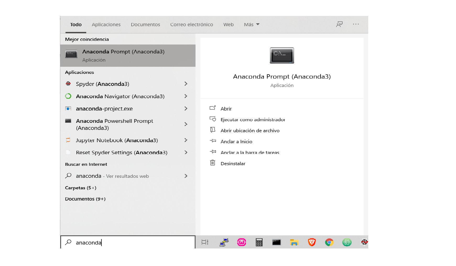
8 | Instalar el paquete Anaconda
9 | Descarga de la pagina oficial https://www.anaconda.com/products/individual
10 | Abrir el prompt anaconda para instalar paquete de yahoo finance
11 |
12 |
13 |
14 |
15 |
16 |
17 |
18 | > Luego, desde el prompt anaconda instalar el paquete de Yahoo Finance para bajar datos de mercado
19 | > Para ello tipear la siguiente linea de codigo:
20 |
21 | ```sh
22 | pip install yfinance
23 | ```
24 |
25 |
26 |
27 |
28 |
29 | # Archivos
30 |
31 | * [PrimerosPasos](https://github.com/gauss314/Bursatil-Argentina-Python/blob/master/analisis%20activo.py) Bajar datos de mercado por activo
32 | * [CCLs](https://github.com/gauss314/Bursatil-Argentina-Python/blob/master/ccls.py) Calculo del CCL para diferentes tickers (GGAL, PAM, YPF, etc)
33 | * [Brechas](https://github.com/gauss314/Bursatil-Argentina-Python/blob/master/brechas.py) TDC oficial, MEP y CCL, Brecha actual CCL-Oficial, MEP-Oficial, CCL-MEP
34 | * [BCRA](https://github.com/gauss314/Bursatil-Argentina-Python/blob/master/bcra.py) +40 Endpoints de series historicas del BCRA (como reservas internacionales, tdc, m2, tasas, etc)
35 | * [Bot de Trading](https://github.com/gauss314/Bursatil-Argentina-Python/blob/master/Bot%20basico%20BTCpy.py) Ejemplo a fines dídácticos de como funciona un bot de trading
36 | * [CAGR idea](https://github.com/gauss314/Bursatil-Argentina-Python/blob/master/CAGR2.py) Ejemplo de estrategia de Holdear las peores o mejores 5 acciones de una lista segun rendimiento de semana previa, idea de @camilocr3 https://twitter.com/camilocr3
37 | * [Futures](https://github.com/gauss314/Bursatil-Argentina-Python/blob/master/CAGR2.py) Comparación de Futuros de commodities como el WTI el oro etc, vs precios y volumenes de "X" dias atras, idea de @lucasgday https://twitter.com/lucasgday
38 | * [Black&Scholes](https://github.com/gauss314/Bursatil-Argentina-Python/blob/master/black_scholes.py) Cálculo de VI en opciones mediante modelo de Black&Scholes y griegas
39 | * [Dolar Blue](https://github.com/gauss314/Bursatil-Argentina-Python/blob/master/blue.py) Scrapper del valor del dolar Blue de todo un año y download en un excel
40 | * [DrawDowns Merval](https://github.com/gauss314/Bursatil-Argentina-Python/blob/master/caidas%20desde%20max%20merval.py) Análisis de las máximas cáidas del panel general del merval (derrape 2018-2020) y sus potenciales upsides hasta maximos
41 | * [MachineLearning KMeans](https://github.com/gauss314/Bursatil-Argentina-Python/blob/master/clusterOIL.py) Clusterización de coeficientes de correlación OIL vs Petroleras
42 | * [Graficos 3D](https://github.com/gauss314/Bursatil-Argentina-Python/blob/master/graf%203D-Points.py) Perfil de volumen-precio en un graf 3D con matplotlib
43 | * [Panel Opciones Byma](https://github.com/gauss314/Bursatil-Argentina-Python/blob/master/opcionesByma.py) Scrapper de la página de Rava a DataFrame y download a excel
44 | * [Transcribir Video de YouTube](https://github.com/gauss314/Bursatil-Argentina-Python/blob/master/transcribir%20video.py) Analizador, contador y comparador de las palabras de un video de youtube
45 | * [Google Sheets / Google Finance](https://github.com/gauss314/Bursatil-Argentina-Python/blob/master/googleSheets.py) Lectura sencilla de tabla de planilla de googlesheet online y pasaje a dataframe
46 |
47 |
48 |
49 |
50 | > Hilo de twitter donde se inició esta idea:
51 | https://twitter.com/JohnGalt_is_www/status/1210981218768044033
52 |
53 |
54 |
55 |
56 |
57 | ## Créditos
58 |
59 | Utilizamos las librerías:
60 | - yfinance https://github.com/ranaroussi/yfinance
61 |
--------------------------------------------------------------------------------
/black_scholes.py:
--------------------------------------------------------------------------------
1 | import math #necesario para calculos como logaritmos, raices, pi, exponentes etc
2 |
3 | #Funcion normal acumulada (es una aproximacion por taylor 6 decimales)
4 | def fi(x):
5 | Pi = 3.141592653589793238;
6 | a1 = 0.319381530;
7 | a2 = -0.356563782;
8 | a3 = 1.781477937;
9 | a4 = -1.821255978;
10 | a5 = 1.330274429;
11 | L = abs(x);
12 | k = 1 / ( 1 + 0.2316419 * L);
13 | p = 1 - 1 / pow(2 * Pi, 0.5) * math.exp( -pow(L, 2) / 2 ) * (a1 * k + a2 * pow(k, 2)
14 | + a3 * pow(k, 3) + a4 * pow(k, 4) + a5 * pow(k, 5) );
15 | if (x >= 0) :
16 | return p
17 | else:
18 | return 1-p
19 |
20 | def normalInv(x):
21 | return ((1/math.sqrt(2*math.pi)) * math.exp(-x*x*0.5))
22 |
23 |
24 | #Funciones de Calculo de primas y griegas
25 | def bsCall(S0, K, r, T, sigma, q=0):
26 | ret = {}
27 | if (S0 > 0 and K > 0 and r >= 0 and T > 0 and sigma > 0):
28 | d1 = ( math.log(S0/K) + (r -q +sigma*sigma*0.5)*T ) / (sigma * math.sqrt(T))
29 | d2 = d1 - sigma*math.sqrt(T)
30 | ret['call'] = math.exp(-q*T) * S0 * fi(d1)- K*math.exp(-r*T)*fi(d2)
31 | ret['delta'] = math.exp(-q*T) * fi(d1)
32 | ret['gamma'] = (normalInv(d1) * math.exp(-q*T)) / (S0 * sigma * math.sqrt(T))
33 | ret['vega'] = 0.01 * S0 * math.exp(-q*T) * normalInv(d1) * math.sqrt(T)
34 | ret['theta'] = (1/365) * ( -((S0*sigma*math.exp(-q*T))/(2*math.sqrt(T))) * normalInv(d1) - r*K*(math.exp(-r*T))*fi(d2) + q*S0*(math.exp(-q*T)) * fi(d1) )
35 | ret['rho'] = 0.01 * K * T * math.exp(-r*T) * fi(d2)
36 | else:
37 | ret['errores']= "Se Ingresaron valores incorrectos"
38 | return ret
39 |
40 |
41 | def bsPut(S0, K, r, T, sigma, q=0):
42 | ret = {}
43 | if (S0 > 0 and K > 0 and r >= 0 and T > 0 and sigma > 0):
44 | d1 = ( math.log(S0/K) + (r -q +sigma*sigma*0.5)*T ) / (sigma * math.sqrt(T))
45 | d2 = d1 - sigma*math.sqrt(T)
46 | ret['put'] = K*math.exp(-r*T)*fi(-d2) - math.exp(-q*T) * S0 * fi(-d1)
47 | ret['delta'] = - math.exp(-q*T) * fi(-d1)
48 | ret['gamma'] = math.exp(-q*T) * normalInv(d1) / (S0 * sigma * math.sqrt(T))
49 | ret['vega'] = 0.01* S0 * math.exp(-q*T) * normalInv(d1) * math.sqrt(T)
50 | ret['theta'] = (1/365) * ( -((S0*sigma*math.exp(-q*T))/(2*math.sqrt(T))) * normalInv(d1) + r*K*(math.exp(-r*T))*fi(-d2) - q*S0*(math.exp(-q*T)) * fi(-d1) )
51 | ret['rho'] = -0.01 * K * T * math.exp(-r*T) * fi(-d2)
52 | else:
53 | ret['errores']= "Se Ingresaron valores incorrectos"
54 | return ret
55 |
56 |
57 | def viCall(S0, K, r, T, prima, q=0):
58 | if (S0 > 0 and K > 0 and r >= 0 and T > 0):
59 | maximasIteraciones = 300
60 | pr_techo = prima
61 | pr_piso = prima
62 | vi_piso = maximasIteraciones
63 | vi = maximasIteraciones
64 | for number in range(1,maximasIteraciones):
65 | sigma = (number)/100
66 | primaCalc = bsCall(S0, K, r, T, sigma, q)['call']
67 | if primaCalc>prima:
68 | vi_piso = number -1
69 | pr_techo = primaCalc
70 | break
71 | else:
72 | pr_piso = primaCalc
73 |
74 | rango = (prima - pr_piso) / (pr_techo - pr_piso)
75 | vi = vi_piso + rango
76 | else:
77 | vi = "No se puede calcular VI porque los valores ingresados son incorrectos"
78 | return(vi)
79 |
80 |
81 | def viPut(S0, K, r, T, prima, q=0):
82 | if (S0 > 0 and K > 0 and r >= 0 and T > 0):
83 | maximasIteraciones = 300
84 | pr_techo = prima
85 | pr_piso = prima
86 | vi_piso = maximasIteraciones
87 | vi = maximasIteraciones
88 | for number in range(1,maximasIteraciones):
89 | sigma = (number)/100
90 | primaCalc = bsPut(S0, K, r, T, sigma, q)['put']
91 | if primaCalc>prima:
92 | vi_piso = number -1
93 | pr_techo = primaCalc
94 | break
95 | else:
96 | pr_piso = primaCalc
97 |
98 | rango = (prima - pr_piso) / (pr_techo - pr_piso)
99 | vi = vi_piso + rango
100 | else:
101 | vi = "No se puede calcular VI porque los valores ingresados son incorrectos"
102 | return(vi)
103 |
104 |
105 |
106 | #INGRESO DE DATOS
107 |
108 | S0 = 100 #Spot subyacente
109 | K = 100 #strike o base del contrato
110 | r = 0.018 #tasa libre de riesgo
111 | T = 30/365 #tiempo en años para expiracion
112 | sigma = 0.2 #volatilidad anualizada
113 | q = 0.01 #dividend yield (ojo los highYield que en USA no se limpian las bases ex div)
114 |
115 |
116 | #CALCULO DE PRIMAS Y GRIEGAS
117 | call = bsCall(S0, K, r, T, sigma, q)
118 | put = bsPut(S0, K, r, T, sigma, q)
119 |
120 |
121 | #IMPRESION EN PANTALLA
122 | print(call)
123 | print(put)
124 |
125 | #CALCULO DE VI DADO PRECIO DE MERCADO
126 | vi = viCall(S0, K, r, T, 2, q)
127 | print(vi)
128 |
129 |
130 |
--------------------------------------------------------------------------------
/concurso_nb.ipynb:
--------------------------------------------------------------------------------
1 | {
2 | "cells": [
3 | {
4 | "cell_type": "code",
5 | "execution_count": 1,
6 | "metadata": {},
7 | "outputs": [],
8 | "source": [
9 | "import pandas as pd\n",
10 | "import tweepy\n",
11 | "import ssl\n",
12 | "ssl._create_default_https_context = ssl._create_unverified_context\n",
13 | "\n",
14 | "consumer_key = \"XXXXXXX\"\n",
15 | "consumer_secret = \"XXXXXXX\"\n",
16 | "access_token = \"XXXXXXX\"\n",
17 | "access_token_secret = \"XXXXXXX\"\n",
18 | "\n",
19 | "# Authentication with Twitter\n",
20 | "auth = tweepy.OAuthHandler(consumer_key, consumer_secret)\n",
21 | "auth.set_access_token(access_token, access_token_secret)\n",
22 | "api = tweepy.API(auth)"
23 | ]
24 | },
25 | {
26 | "cell_type": "code",
27 | "execution_count": 2,
28 | "metadata": {},
29 | "outputs": [],
30 | "source": [
31 | "def tiene_digitos(texto):\n",
32 | " digitos = ['1','2','3','4','5','6','7','8','9','0']\n",
33 | " r = False\n",
34 | " for digito in digitos:\n",
35 | " res = texto.find(digito)\n",
36 | " if res>-1:\n",
37 | " r = True\n",
38 | "\n",
39 | " return r"
40 | ]
41 | },
42 | {
43 | "cell_type": "code",
44 | "execution_count": 3,
45 | "metadata": {},
46 | "outputs": [],
47 | "source": [
48 | "def limpiar_puntos(valor):\n",
49 | " if len(valor.split('.')) > 2:\n",
50 | " num = '.'.join(valor.split('.')[:2])\n",
51 | " return num\n",
52 | " else:\n",
53 | " return valor"
54 | ]
55 | },
56 | {
57 | "cell_type": "code",
58 | "execution_count": 4,
59 | "metadata": {},
60 | "outputs": [],
61 | "source": [
62 | "def eliminar_alfas(palabra):\n",
63 | " for letra in palabra:\n",
64 | " if letra not in '0123456789.,':\n",
65 | " palabra = palabra.replace(letra,'')\n",
66 | "\n",
67 | " return palabra"
68 | ]
69 | },
70 | {
71 | "cell_type": "code",
72 | "execution_count": 5,
73 | "metadata": {},
74 | "outputs": [],
75 | "source": [
76 | "def barrer_tw(tweet_id):\n",
77 | "\n",
78 | " replies=[]\n",
79 | " for tweet in tweepy.Cursor(api.search,q='to:'+'JohnGalt_is_www', result_type='recent', timeout=999999).items(1000):\n",
80 | " if hasattr(tweet, 'in_reply_to_status_id_str'):\n",
81 | " if (tweet.in_reply_to_status_id_str==tweet_id):\n",
82 | " replies.append(tweet)\n",
83 | "\n",
84 | " tuits = []\n",
85 | " for tweet in replies:\n",
86 | " texto = tweet.text.replace('\\n', ' ')\n",
87 | " texto = texto.replace('@JohnGalt_is_www @Jotatrader_ok ','')\n",
88 | " palabras = texto.split()\n",
89 | "\n",
90 | " valores = [palabra for palabra in texto.split() if tiene_digitos(palabra)]\n",
91 | " valores = [ (v.replace('$', '').replace(',','.')) for v in valores]\n",
92 | " valores_num = [ float(limpiar_puntos(eliminar_alfas(v))) for v in valores]\n",
93 | " valores_num.sort()\n",
94 | " if len(valores_num)==2:\n",
95 | " if (valores_num[0]>50) & (valores_num[1]>50):\n",
96 | " row = {'user': tweet.user.screen_name, 'GGAL': valores_num[0], 'YPFD':valores_num[1]}\n",
97 | " tuits.append(row)\n",
98 | " \n",
99 | " df = pd.DataFrame(tuits)\n",
100 | " return df"
101 | ]
102 | },
103 | {
104 | "cell_type": "code",
105 | "execution_count": 6,
106 | "metadata": {},
107 | "outputs": [],
108 | "source": [
109 | "df_1 = barrer_tw('1374051527682326535')\n",
110 | "df_2 = barrer_tw('1374051528928034822')"
111 | ]
112 | },
113 | {
114 | "cell_type": "code",
115 | "execution_count": 7,
116 | "metadata": {},
117 | "outputs": [
118 | {
119 | "data": {
120 | "text/html": [
121 | "
 14 |
14 |