├── Installation
├── .gitkeep
└── install_anaconda_python.md
├── Pratice Guide
├── .gitkeep
└── research_guide_for_fyp.md
├── ML from Scratch
├── README.md
├── Linear Regression
│ ├── .gitkeep
│ ├── salaries.csv
│ ├── README.md
│ └── Predict-Salary-based-on-Experience---Linear-Regression.ipynb
├── Random Forest
│ └── README.md
├── Support Vector Machine
│ └── README.md
├── Decision Tree
│ └── README.md
├── KNN
│ └── README.md
├── Naive Bayes
│ └── README.md
├── K Means Clustering
│ └── README.md
└── Logistic Regression
│ └── README.md
├── Reality vs Expectation
├── .gitkeep
└── Is AI Overhyped? Reality vs Expectation.md
├── Mathematical Implementation
├── .gitkeep
├── PCA.md
├── Compute MSA, RMSE, and MAE.md
└── confusion_matrix.md
├── Machine Learning from Beginner to Advanced
├── .gitkeep
├── Data Cleaning and Pre-processing.md
├── data_preparation.md
├── Introduction to ML and AI.md
├── Key terms used in ML.md
├── Regression Performance Metrics.md
├── mathematics_ai_ml_history_motivation.md
└── Classification Performance Metrics.md
├── LICENSE
└── README.md
/Installation/.gitkeep:
--------------------------------------------------------------------------------
1 |
--------------------------------------------------------------------------------
/Pratice Guide/.gitkeep:
--------------------------------------------------------------------------------
1 |
--------------------------------------------------------------------------------
/ML from Scratch/README.md:
--------------------------------------------------------------------------------
1 |
--------------------------------------------------------------------------------
/Reality vs Expectation/.gitkeep:
--------------------------------------------------------------------------------
1 |
--------------------------------------------------------------------------------
/Mathematical Implementation/.gitkeep:
--------------------------------------------------------------------------------
1 |
--------------------------------------------------------------------------------
/ML from Scratch/Linear Regression/.gitkeep:
--------------------------------------------------------------------------------
1 |
--------------------------------------------------------------------------------
/Machine Learning from Beginner to Advanced/.gitkeep:
--------------------------------------------------------------------------------
1 |
--------------------------------------------------------------------------------
/Mathematical Implementation/PCA.md:
--------------------------------------------------------------------------------
1 | Working............
2 |
--------------------------------------------------------------------------------
/Mathematical Implementation/Compute MSA, RMSE, and MAE.md:
--------------------------------------------------------------------------------
1 |
2 |
--------------------------------------------------------------------------------
/Machine Learning from Beginner to Advanced/Data Cleaning and Pre-processing.md:
--------------------------------------------------------------------------------
1 |
2 |
--------------------------------------------------------------------------------
/ML from Scratch/Linear Regression/salaries.csv:
--------------------------------------------------------------------------------
1 | Years of Experience,Salary
2 | 1.1,39343
3 | 1.3,46205
4 | 1.5,37731
5 | 2,43525
6 | 2.2,39891
7 | 2.9,56642
8 | 3,60150
9 | 3.2,54445
10 | 3.2,64445
11 | 3.7,57189
12 | 3.9,63218
13 | 4,55794
14 | 4,56957
15 | 4.1,57081
16 | 4.5,61111
17 | 4.9,67938
18 | 5.1,66029
19 | 5.3,83088
20 | 5.9,81363
21 | 6,93940
22 | 6.8,91738
23 | 7.1,98273
24 | 7.9,101302
25 | 8.2,113812
26 | 8.7,109431
27 | 9,105582
28 | 9.5,116969
29 | 9.6,112635
30 | 10.3,122391
31 | 10.5,121872
32 |
--------------------------------------------------------------------------------
/LICENSE:
--------------------------------------------------------------------------------
1 | MIT License
2 |
3 | Copyright (c) 2022 Sunil Ghimire
4 |
5 | Permission is hereby granted, free of charge, to any person obtaining a copy
6 | of this software and associated documentation files (the "Software"), to deal
7 | in the Software without restriction, including without limitation the rights
8 | to use, copy, modify, merge, publish, distribute, sublicense, and/or sell
9 | copies of the Software, and to permit persons to whom the Software is
10 | furnished to do so, subject to the following conditions:
11 |
12 | The above copyright notice and this permission notice shall be included in all
13 | copies or substantial portions of the Software.
14 |
15 | THE SOFTWARE IS PROVIDED "AS IS", WITHOUT WARRANTY OF ANY KIND, EXPRESS OR
16 | IMPLIED, INCLUDING BUT NOT LIMITED TO THE WARRANTIES OF MERCHANTABILITY,
17 | FITNESS FOR A PARTICULAR PURPOSE AND NONINFRINGEMENT. IN NO EVENT SHALL THE
18 | AUTHORS OR COPYRIGHT HOLDERS BE LIABLE FOR ANY CLAIM, DAMAGES OR OTHER
19 | LIABILITY, WHETHER IN AN ACTION OF CONTRACT, TORT OR OTHERWISE, ARISING FROM,
20 | OUT OF OR IN CONNECTION WITH THE SOFTWARE OR THE USE OR OTHER DEALINGS IN THE
21 | SOFTWARE.
22 |
--------------------------------------------------------------------------------
/Machine Learning from Beginner to Advanced/data_preparation.md:
--------------------------------------------------------------------------------
1 | # 1. Data Quality Inspection
2 |
3 | 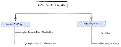
4 |
5 |
6 | The two most popular approach to data quality inspection is: Data Profiling and Data visualization
7 |
8 | ## 1.1. Data Profiling
9 |
10 | Data profiling is reviewing source data, understanding structure, content, and interrelationships, and identifying potential for data projects
11 |
12 | Data profiling is a crucial part of
13 |
14 | - Data warehouse and business intelligence (DW/BI) projects—data profiling can uncover data quality issues in data sources, and what needs to be corrected in ETL.
15 | - Data conversion and migration projects—data profiling can identify data quality issues, which you can handle in scripts and data integration tools copying data from source to target. It can also uncover new requirements for the target system.
16 | - Source system data quality projects—data profiling can highlight data that suffers from serious or numerous quality issues, and the source of the issues (e.g. user inputs, errors in interfaces, data corruption).
17 |
18 | ### 1.1.1. Data profiling involves:
19 |
20 | - Collecting descriptive statistics like min, max, count, and sum.
21 | - Collecting data types, length, and recurring patterns.
22 | - Tagging data with keywords, descriptions, or categories.
23 | - Performing data quality assessment, risk of performing joins on the data.
24 | - Discovering metadata and assessing its accuracy.
25 | - Identifying distributions, key candidates, foreign-key candidates, functional dependencies, embedded value dependencies, and performing inter-table analysis
26 |
27 | ### 1.1.2. Data profiling involves:
28 | Data profiling collects statistics and meta-information about available data that provide insight into the content of data sets
29 |
--------------------------------------------------------------------------------
/Pratice Guide/research_guide_for_fyp.md:
--------------------------------------------------------------------------------
1 | # PART 1: The Reflective Individual Report
2 |
3 | **I. Finding a research topic:- approx 500 words.**
4 | In this task identify your topic and explain how you crafted your research project, selected research tools and search techniques, and which library Library Collections did you explore.
5 |
6 | **Areas that can be covered include**:
7 | * What is your chosen research topic?
8 | * How and why did you choose it?
9 | * What is your research aims and objectives?
10 | * What specific techniques and strategies did you use for finding relevant information?
11 | * What specific library search tools did you use and why?
12 | * What did you learn about finding information on your topic or in your discipline?
13 | * Was it necessary to move outside your discipline to find sufficient sources?
14 |
15 | **II. Professional Activities:- Approx 500 words.**
16 | In this task, you have to show a reflection on a wide range of professional research development activities and responsibilities, through your own self-discovery…
17 |
18 | **Areas which can be covered included:**
19 | * Student’s research tasks and schedule including for example a Gantt Chart
20 | * How did you fit in the dependent researcher role?
21 | * Any Challenges you faced and how did you tackle them?
22 |
23 | **III. Literature Review:- Approx 1500 words.**
24 | This task brings together the main themes of the modules and requires you to build a portfolio from your literature collections.
25 |
26 | **Areas which can be covered included:**
27 | * A mind map of your research topic
28 | * What tools and resources did you use to develop the mind map
29 | * A brief summary of your literature review with proper citation
30 | * What resources and techniques did you use to write your literature review
31 | * Did you have any reason for not selecting specific resources, even though they appeared promising?
32 | * What is your research method and what are the practical steps you used to complete your research?
33 | * Comment on the feasibility of your chosen method including challenges and recommendations.
34 |
35 | **IV. Refection of Research Project:- Approx 500 words**
36 | Here is your opportunity to bring your achievements and contributions in a portfolio of the work done in a professional manner and reflected upon the relevance of the various activities.
37 |
38 | Summarise how you have reflected on your learning and development whilst on a research project. Demonstrate awareness of your personal strengths and weaknesses and the ability to adapt to the independent research process and how you would engage further in continuing self-development.
39 |
40 | **Areas which can be covered included:**
41 | * What was the achievement during this research?
42 | * What did you learn about your own research process and style?
43 | * What expertise have you gained as a researcher?
44 | * What do you still need to learn?
45 | * What would you change about your process if you had another chance?
46 | * Any recommendations
47 |
48 | **PART 2: The Reflective Notebook File**
49 | The final 50% will be awarded for your notebook file.
50 |
51 | Note: Your work needs to be fully referenced, which is good practice for your dissertation.
52 |
53 | If you have any queries, feedback, or suggestions then you can leave a comment or mail on info@sunilghimire.com.np. See you in the next tutorial.
54 |
55 | ### **Stay safe !! Happy Learning !!!**
56 |
57 | _**STEPHEN HAWKING ONCE SAID, “The thing about smart people is that they seem like crazy people to dumb people.”**_
58 |
--------------------------------------------------------------------------------
/Machine Learning from Beginner to Advanced/Introduction to ML and AI.md:
--------------------------------------------------------------------------------
1 | # INTRODUCTION TO ARTIFICIAL INTELLIGENCE & MACHINE LEARNING
2 |
3 |
4 | Artificial intelligence can be interpreted as adding human intelligence in a machine. Artificial intelligence is not a system but a discipline that focuses on making machine smart enough to tackle the problem like the human brain does. The ability to learn, understand, imagine are the qualities that are naturally found in Humans. Developing a system that has the same or better level of these qualities artificially is termed as Artificial Intelligence.
5 |
6 | Machine Learning is a subset of AI. That is, all machine learning counts as AI, but not all AI counts as machine learning. Machine learning refers to the system that can learn by themselves. **Machine learning is the study of computer algorithms that comprises of algorithms and statistical models that allow computer programs to automatically improve through experience.**
7 |
8 | > “Machine learning is the tendency of machines to learn from data analysis and achieve Artificial Intelligence.”
9 |
10 | **Machine Learning** is the science of getting computers to act by feeding them data and letting them learn a few tricks on their own without being explicitly programmed.
11 |
12 | ## DIFFERENCE BETWEEN MACHINE LEARNING AND ARTIFICIAL INTELLIGENCE
13 | * Artificial intelligence focuses on Success whereas Machine Learning focuses on Accuracy
14 | * AI is not a system, but it can be implemented on system to make system intelligent. ML is a system that can extract knowledge from datasets
15 | * AI is used in decision making whereas ML is used in learning from experience
16 | * AI mimics human whereas ML develops self-learning algorithm
17 | * AI leads to wisdom or intelligence whereas ML leads to knowledge or experience
18 | * Machine Learning is one of the way to achieve Artificial Intelligence.
19 |
20 | ## TYPES OF MACHINE LEARNING
21 | * Supervised Learning
22 | * Unsupervised learning
23 | * Reinforced Learning
24 |
25 | **Supervised** means to oversee or direct a certain activity and make sure it is done correctly. In this type of learning the machine learns under guidance. So, at school or teachers guided us and taught us similarly in supervised learning machines learn by feeding them label data and explicitly telling them that this is the input and this is exactly how the output must look. So, the teacher, in this case, is the training data.
26 | * Linear Regression
27 | * Logistic Regression
28 | * Support Vector Machine
29 | * Naive Bayes Classifier
30 | * Artificial Neural Networks, etc
31 |
32 | **Unsupervised** means to act without anyone’s supervision or without anybody’s direction. Now, here the data is not labeled. There is no guide and the machine has to figure out the data set given and it has to find hidden patterns in order to make predictions about the output. An example of unsupervised learning is an adult-like you and me. We do not need a guide to help us with our daily activities. We can figure things out on our own without any supervision.
33 | * K-means clustering
34 | * Principal Component Analysis
35 | * Generative Adversarial Networks
36 |
37 | **Reinforcement** means to establish or encourage a pattern of behavior. It is a learning method wherein an agent learns by producing actions and discovers errors or rewards. Once the agent gets trained it gets ready to predict the new data presented to it.
38 |
39 | Let’s say a child is born. What will he do? But after some months or years, he tries to walk. So here he basically follows the hit and trial concept because he is new to the surroundings and the only way to learn is experience. We notice baby stretching and kicking his legs and starts to roll over. Then he starts crawling. He then tries to stand up but he fails in doing so for many attempts. Then the baby will learn to support all his weight when held in a standing position. This is what reinforcement learning is.
40 |
--------------------------------------------------------------------------------
/Machine Learning from Beginner to Advanced/Key terms used in ML.md:
--------------------------------------------------------------------------------
1 | # KEY TERMS USED IN MACHINE LEARNING
2 |
3 | Before starting tutorials on machine learning, we came with an idea of providing a brief definition of key terms used in Machine Learning. These key terms will be regularly used in our coming tutorials on machine learning from scratch and will also be used in further higher courses. So let’s start with the term Machine Learning:
4 |
5 | ## MACHINE LEARNING
6 | Machine learning is the study of computer algorithms that comprises of algorithms and statistical models that allow computer programs to automatically improve through experience. It is the science of getting computers to act by feeding them data and letting them learn a few tricks on their own without being explicitly programmed.
7 |
8 | > TYPES OF MACHINE LEARNING
9 | > **Do you want to know about supervised, unsupervised and reinforcement learning?** [Read More](https://github.com/ghimiresunil/Implementation-of-Machine-Learning-Algorithm-from-Scratch/blob/main/Machine%20Learning%20from%20Beginner%20to%20Advanced/Introduction%20to%20ML%20and%20AI.md)
10 |
11 | ## CLASSIFICATION
12 | Classification, a sub-category of supervised learning, is defined as the process of separating data into distinct categories or classes. These models are built by providing a labeled dataset and making the algorithm learn so that it can predict the class when new data is provided. The most popular classification algorithms are Decision Tree, SVM.
13 |
14 | We have two types of learners in respective classification problems:
15 |
16 | * Lazy Learners: As the name suggests, such kind of learners waits for the testing data to be appeared after storing the training data. Classification is done only after getting the testing data. They spend less time on training but more time on predicting. Examples of lazy learners are K-nearest neighbor and case-based reasoning.
17 |
18 | * Eager Learners: As opposite to lazy learners, eager learners construct a classification model without waiting for the testing data to be appeared after storing the training data. They spend more time on training but less time on predicting. Examples of eager learners are Decision Trees, Naïve Bayes, and Artificial Neural Networks (ANN).
19 |
20 | **_Note_**: We will study these algorithms in the coming tutorials.
21 |
22 | ## REGRESSION
23 | While classification deals with predicting discrete classes, regression is used in predicting continuous numerical valued classes. Regression is also falls under supervised learning generally used to answer “How much?” or “How many?”. Regressions create relationships and correlations between different types of data. Linear Regression is the most common regression algorithm.
24 |
25 | Regression models are of two types:
26 |
27 | * Simple regression model: This is the most basic regression model in which predictions are formed from a single, univariate feature of the data.
28 | * Multiple regression model: As the name implies, in this regression model the predictions are formed from multiple features of the data.
29 | ## CLUSTERING
30 | Cluster is defined as groups of data points such that data points in a group will be similar or related to one another and different from the data points of another group. And the process is known as clustering. The goal of clustering is to determine the intrinsic grouping in a set of unlabelled data. Clustering is a form of unsupervised learning since it doesn’t require labeled data.
31 |
32 | ## DIMENSIONALITY
33 | The dimensionality of a data set is the number of attributes or features that the objects in the dataset have. In a particular dataset, if there are number of attributes, then it can be difficult to analyze such dataset which is known as curse of dimensionality.
34 |
35 | ## CURSE OF DIMENSIONALITY
36 | Data analysis becomes difficult as the dimensionality of data set increases. As dimensionality increases, the data becomes increasingly sparse in the space that it occupies.
37 |
38 | * For classification, there will not be enough data objects to allow the creation of model that reliably assigns a class to all possible objects.
39 | * For clustering, the density and distance between points which are critical for clustering becomes less meaningful.
40 | 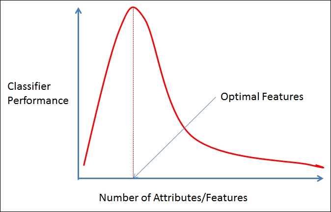
41 |
42 |
43 | ## UNDERFITTING
44 | A machine learning algorithm is said to have underfitting when it can’t capture the underlying trend of data. It means that our model doesn’t fit the data well enough. It usually happens when we have fewer data to build a model and also when we try to build a linear model with non-linear data when using a less complex model.
45 |
46 | ## OVERFITTING
47 | When a model gets trained with so much data, it starts learning from the noise and inaccurate data entries in our dataset. The cause of overfitting is non-parametric and non-linear methods. We use cross-validation to reduce overfitting which allows you to tune hyperparameters with only your original training set. This allows you to keep your test set as truly unseen dataset for selecting your final model.
48 |
49 | 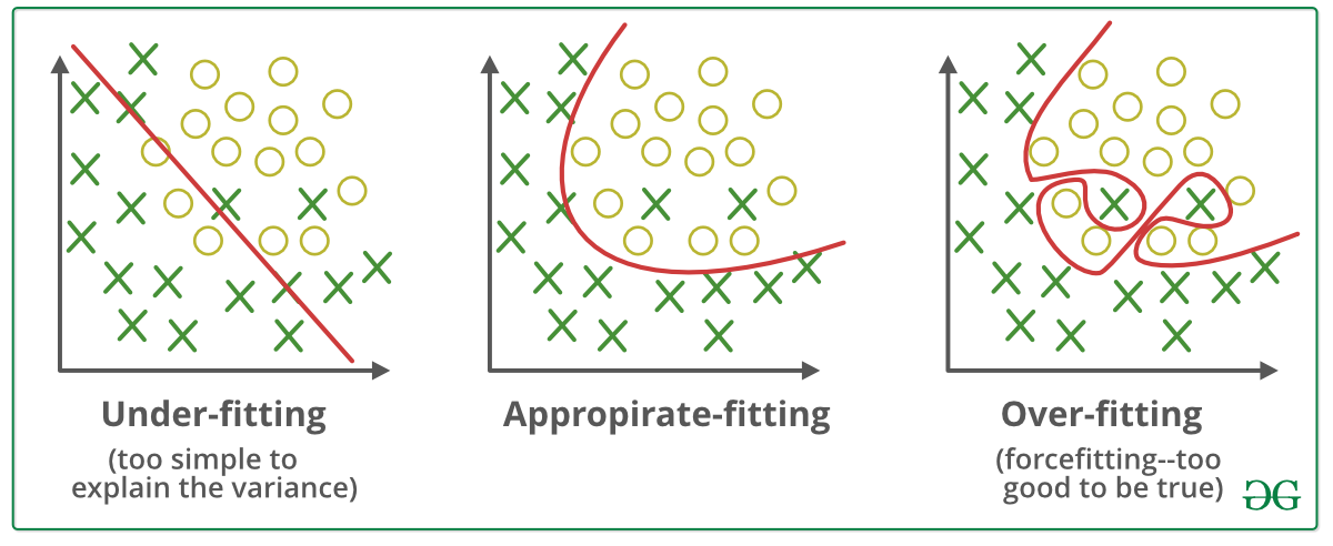
50 |
51 |
--------------------------------------------------------------------------------
/Machine Learning from Beginner to Advanced/Regression Performance Metrics.md:
--------------------------------------------------------------------------------
1 | # Performance Metrics: Regression Model
2 |
3 | Today I am going to discuss Performance Metrics, and this time it will be Regression model metrics. As in my previous blog, I have discussed Classification Metrics, this time its Regression. I am going to talk about the 5 most widely used Regression metrics:
4 |
5 | Let’s understand one thing first and that is the Difference between Classification and Regression:
6 |
7 | 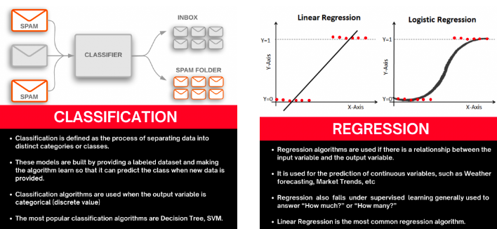
8 |
9 | ## WHAT IS AN ERROR?
10 | Any deviation from the actual value is an error.
11 |
12 | Error = $Y_{actual} - Y_{predicted}$
13 |
14 | So keeping this in mind, we have understood the requirement of the metrics, let’s deep dive into the methods we can use to find out ways to understand our model’s performance.
15 |
16 | ### Mean Squared Error (MSE)
17 |
18 | Let’s try to breakdown the name, it says Mean, it says Squared, it says Error. We know what Error is, from the above explanation, we know what square is. We square the Error, and then we know what the Mean is. So we take the mean of all the errors which are squared and added.
19 |
20 | First question should arise is, why are we doing a Square? Why can we not take the error directly?
21 |
22 | Let’s take the height example, My model predicted 167cm whereas my actual value is 163cm, so the deviation is of +5cm. Let’s take another example where my predicted height is 158cm and my actual height is 163cm. Now, my model made a mistake of -5cm.
23 |
24 | Now let’s find Mean Error for 2 points, so the calculation states [+5 + (-5)]/2 = 0
25 |
26 | This shows that my model has 0 error, but is that true? No right? So to avoid such problems we have to take square to get rid of the Sign of the error.
27 |
28 | So let’s see the formulation of this Metric:
29 |
30 | MSE = $\frac{1}{n}\Sigma_{i=1}^n(y_i - \hat{y_i})^2$
31 |
32 | Where,
33 |
34 | n = total otal number of data points
35 | $y_i$ = actual value
36 | $\hat{y_i}$ = predicted value
37 |
38 | Root Mean Squared Error (RMSE)
39 |
40 | Now as we all understood what MSE is, it is pretty much obvious that taking root of the equation will give us RMSE. Let’s see the formula first.
41 |
42 | RMSE = $\sqrt{\Sigma_{i=1}^n \frac{(\hat{y_i} - y_i)^2}{n}}$
43 |
44 | Where,
45 |
46 | n = total otal number of data points
47 | $y_i$ = actual value
48 | $\hat{y_i}$ = predicted value
49 |
50 | Now the question is, if we already have the MSE, why we require RMSE?
51 |
52 | Let’s try to understand it with example. Take the above example of the 2 data points and calculate MSE and RMSE for them,
53 |
54 | MSE = $\[(5)^2 + (-5)^2\]/2 = 50 / 2 = 25 $
55 |
56 | RMSE = Sqrt(MSE) = $(25)^{0.5}$ = 5
57 |
58 | Now, you tell among these values which one is more accurate and relevant to the actual error of the model?
59 |
60 | RMSE right? So in actual Squaring off, the values increase them exponentially. While not taking a root might affect our understanding that where my model is actually making mistakes.
61 |
62 | ### Mean Absolute Error (MAE)
63 |
64 | Now, I am sure you might have given this a thought, why squaring? Why not just taking the Absolute value of them, so here we have it. Everything stays the same, the only difference is, we take the Absolute value of our error, this also takes care of the sign issues we had earlier. So let’s look into the formula :
65 |
66 | MAE = $ \frac{1}{N} \Sigma_{i=1}^n|y_i - \hat{y_i}|$
67 |
68 | Where,
69 |
70 | n = total otal number of data points
71 | $y_i$ = actual value
72 | $\hat{y_i}$ = predicted value
73 |
74 | #### MAE VS RMSE
75 |
76 | Let’s understand, MAE and RMSE can be used together to diagnose the variation in the errors in a set of forecasts. RMSE will always be larger or equal to the MAE. The greater difference between them, the greater the variance in the individual errors in the sample. If the RMSE=MAE, then all the errors are of the same magnitude.
77 |
78 | Errors $[2, -3, 5, 120, -116, 197]$
79 | RMSE = 115.5
80 | MAE = 88.6
81 |
82 | If we see the difference, RMSE has a higher value then MAE, which states that RMSE gives more importance to higher error due to squaring the values.
83 |
84 | ### Mean Absolute Percentage Error (MAPE)
85 |
86 | MAPE = $\frac{1}{n}\Sigma_{i=1}^n \frac{|y_i - \hat{y_i}|}{y_i} \times 100 \%$
87 |
88 | Where,
89 |
90 | n = total otal number of data points
91 | $y_i$ = actual value
92 | $\hat{y_i}$ = predicted value
93 |
94 | MAPE represents the error in percentage and therefore it’s not relative to the size of the numbers in the data itself, whereas any other performance metrics in the regression model.
95 |
96 | ### $R^2$ or Coefficient of Determination
97 |
98 | It is the Ratio of the MSE (Prediction Error) and Baseline Variance of target Variable, here baseline is the deviation of our Y values from the Mean value.
99 |
100 | The metric helps us to compare our current model with constant baseline value (i.e. mean) and tells us how much our model is better, R2 is always less than 1, and it doesn’t matter how large or small the errors are R2 is always less than 1. Let’s See the Formulation:
101 |
102 | $R^2$ = $1- \frac{SS_{RES}}{SS_{TOT}} = 1 - \frac{\Sigma_{i}(y_i - \hat{y_i})^2}{\Sigma_{i}(y_i - \bar{y_i})^2}$
103 |
--------------------------------------------------------------------------------
/Reality vs Expectation/Is AI Overhyped? Reality vs Expectation.md:
--------------------------------------------------------------------------------
1 | # IS AI OVERHYPED? REALITY VS EXPECTATION
2 |
3 |
4 |
5 |
6 | Humans are the most intelligent species found on Earth. The ability to learn, understand, imagine are the qualities that are naturally found in Humans. Developing a system that has the same or better level of these qualities artificially is termed as Artificial Intelligence. Before talking about AI hype, let’s go through brief history of AI.
7 |
8 | ## HISTORY
9 |
10 | The beginning of modern AI started when the term “Artificial Intelligence” was coined in 1956, at a conference at Dartmouth College, in Hanover. Government funding and interest increased but expectations exceeded the reality which led to AI Winter from 1974 to 1980. British government started funding again to compete with the Japanese but couldn’t stop the 2nd AI winter which occurred from 1987 to 1993.
11 |
12 | 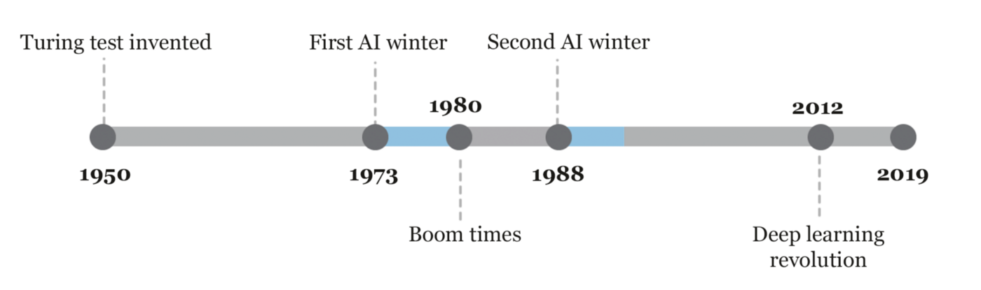
13 |
14 | The field has come a very long way in the past decade. The 10s were the hottest AI summer with tech giants like Google, Facebook, Microsoft repeatedly touting AI’s abilities.
15 |
16 | 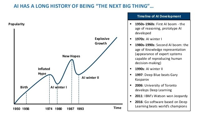
17 |
18 | After the development of higher processing power like GPU, TPU in 10s, Deep Learning made huge jumps. Neural networks offered better results than other algorithms when used on the same data. Talking about the achievement because of Deep learning, Alexa and Siri understanding your voice, Spotify, and Netflix recommending what you watch next, Facebook tagging all your friends in a photo automatically are the remarkable one. With the continuous progress in speed, memory capacity, Quantum Computing performance of AI is being enhanced gradually. Simulations that usually take months are available in days, hours, or less.
19 |
20 | ## CURRENT SCENARIO
21 |
22 | Albert Einstein had once said, “The measure of intelligence is the ability to change”. AI, which started in the 1950s, is aimed at creating a machine that can imitate human behavior with great proficiency. And the question is how AI handles things beyond Human’s imagination? Apart from all the achievements so far in the field of AI, expectations are unreasonably high rather than understanding how it works. Most of the Tech leaders excite people with claims that AI will replace humans but the reality is we do not have the ability to create an AI controlling a robot that can peel an orange.
23 |
24 | In recent years, there’s been intense hype about AI but we aren’t even near living up to the public expectation. Self-driving cars and health care are currently the most hyped areas of artificial intelligence, the most challenging and are taking much longer than the optimistic timetables. AI is still in its infancy, but people are expecting amazing advancements in the next few years like in movies.
25 |
26 | Business-oriented companies are brainwashing or stimulating customers by using AI as a marketing term. Companies deploy some small AI project in their products in a commercial setting. Nowadays, AI is being forcefully tagged in consumer products, like AI Fan, AI fridge, and even AI Toilet. The below picture shows the use of “Artificial Intelligence” in marketing and related key terms.
27 |
28 | ## CHANGE YOUR MIND
29 |
30 | AI is gaining more attention among students and researchers. But, people still don’t realize that they can’t become an expert using stuff like PyTorch, TensorFlow etc. Implementing built-in models with frameworks like Keras, Tensorflow, and Scikit is not unique and special, especially, when we are following an online tutorial and simply changing the data to ours. Coming up and understanding the things behind those architectures is extremely hard. We need a full understanding of probability and statistics, information theory, calculus, etc to just grasp the main ideas.
31 |
32 | AI components are made up of mathematically proven methods or implementation which are coded to work on data. The use of AI depends upon the type of problems they are designed to work on. If ML doesn’t work for you, it’s because you’re not using it right, not because the methods are wrong.
33 |
34 | A routine job that doesn’t require a brain is sure to be replaced by AI. It’s not going to close the job opportunity but will open the different sets of skilled jobs. Let’s take an example of self-driving cars. General Motors, Google’s Waymo, Toyota, Honda, and Tesla are making self-driving cars. After its success, drivers’ jobs will disappear but new job roles of creating and maintaining them will open. Humanity has to evolve towards being more intelligent and it’s the right time.
35 |
36 |
37 | ## CONCLUSION
38 |
39 | We currently call AI as Big Data & Machine Learning. We are focused on finding patterns and predicting the near future trends but AI completely fails when it comes to generating explanations. Reality is, we can’t still trust the decisions of AI in highly-valued & highly-risked domains like finance, healthcare, and energy where even 0.01% accuracy matters.
40 |
41 | With all things taken into consideration, it is sure that AI hype will gradually decrease when people realize we are still using “pseudo-AI” where the fact is humans are operating AI behind the scenes. Though AI has been bookended by fear, doubt, and misinformation, AI hype doesn’t seem to come to an end sooner.
42 |
--------------------------------------------------------------------------------
/ML from Scratch/Linear Regression/README.md:
--------------------------------------------------------------------------------
1 | # LINEAR REGRESSION FROM SCRATCH
2 |
3 | 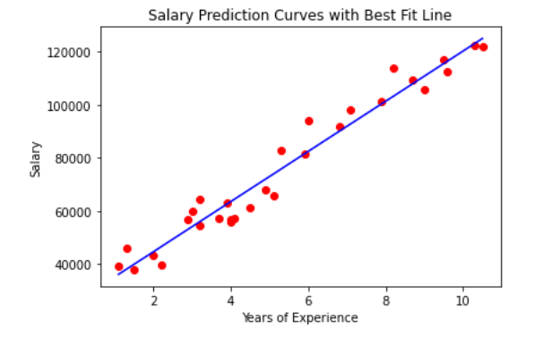
4 |
5 | Regression is the method which measures the average relationship between two or more continuous variables in term of the response variable and feature variables. In other words, regression analysis is to know the nature of the relationship between two or more variables to use it for predicting the most likely value of dependent variables for a given value of independent variables. Linear regression is a mostly used regression algorithm.
6 |
7 | For more concrete understanding, let’s say there is a high correlation between day temperature and sales of tea and coffee. Then the salesman might wish to know the temperature for the next day to decide for the stock of tea and coffee. This can be done with the help of regression.
8 |
9 | The variable, whose value is estimated, predicted, or influenced is called a dependent variable. And the variable which is used for prediction or is known is called an independent variable. It is also called explanatory, regressor, or predictor variable.
10 |
11 | ## 1. LINEAR REGRESSION
12 |
13 | Linear Regression is a supervised method that tries to find a relation between a continuous set of variables from any given dataset. So, the problem statement that the algorithm tries to solve linearly is to best fit a line/plane/hyperplane (as the dimension goes on increasing) for any given set of data.
14 |
15 | This algorithm use statistics on the training data to find the best fit linear or straight-line relationship between the input variables (X) and output variable (y). Simple equation of Linear Regression model can be written as:
16 |
17 | ```
18 | Y=mX+c ; Here m and c are calculated on training
19 | ```
20 |
21 | In the above equation, m is the scale factor or coefficient, c being the bias coefficient, Y is the dependent variable and X is the independent variable. Once the coefficient m and c are known, this equation can be used to predict the output value Y when input X is provided.
22 |
23 | Mathematically, coefficients m and c can be calculated as:
24 |
25 | ```
26 | m = sum((X(i) - mean(X)) * (Y(i) - mean(Y))) / sum( (X(i) - mean(X))^2)
27 | c = mean(Y) - m * mean(X)
28 | ```
29 | 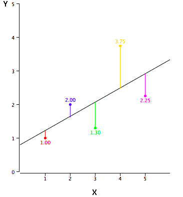
30 |
31 | As you can see, the red point is very near the regression line; its error of prediction is small. By contrast, the yellow point is much higher than the regression line and therefore its error of prediction is large. The best-fitting line is the line that minimizes the sum of the squared errors of prediction.
32 |
33 | ## 1.1. LINEAR REGRESSION FROM SCRATCH
34 |
35 | We will build a linear regression model to predict the salary of a person on the basis of years of experience from scratch. You can download the dataset from the link given below. Let’s start with importing required libraries:
36 |
37 | ```
38 | %matplotlib inline
39 | import numpy as np
40 | import matplotlib.pyplot as plt
41 | import pandas as pd
42 | ```
43 |
44 | We are using dataset of 30 data items consisting of features like years of experience and salary. Let’s visualize the dataset first.
45 |
46 | ```
47 | dataset = pd.read_csv('salaries.csv')
48 |
49 | #Scatter Plot
50 | X = dataset['Years of Experience']
51 | Y = dataset['Salary']
52 |
53 | plt.scatter(X,Y,color='blue')
54 | plt.xlabel('Years of Experience')
55 | plt.ylabel('Salary')
56 | plt.title('Salary Prediction Curves')
57 | plt.show()
58 | ```
59 | 
60 |
61 | ```
62 | def mean(values):
63 | return sum(values) / float(len(values))
64 |
65 | # initializing our inputs and outputs
66 | X = dataset['Years of Experience'].values
67 | Y = dataset['Salary'].values
68 |
69 | # mean of our inputs and outputs
70 | x_mean = mean(X)
71 | y_mean = mean(Y)
72 |
73 | #total number of values
74 | n = len(X)
75 |
76 | # using the formula to calculate the b1 and b0
77 | numerator = 0
78 | denominator = 0
79 | for i in range(n):
80 | numerator += (X[i] - x_mean) * (Y[i] - y_mean)
81 | denominator += (X[i] - x_mean) ** 2
82 |
83 | b1 = numerator / denominator
84 | b0 = y_mean - (b1 * x_mean)
85 |
86 | #printing the coefficient
87 | print(b1, b0)
88 | ```
89 | Finally, we have calculated the unknown coefficient m as b1 and c as b0. Here we have b1 = **9449.962321455077** and b0 = **25792.20019866869**.
90 |
91 | Let’s visualize the best fit line from scratch.
92 |
93 | 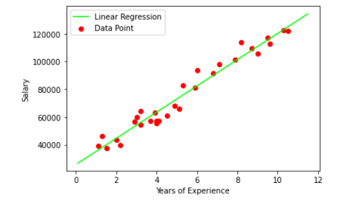
94 |
95 | Now let’s predict the salary Y by providing years of experience as X:
96 |
97 | ```
98 | def predict(x):
99 | return (b0 + b1 * x)
100 | y_pred = predict(6.5)
101 | print(y_pred)
102 |
103 | Output: 87216.95528812669
104 | ```
105 | ### 1.2. LINEAR REGRESSION USING SKLEARN
106 |
107 | ```
108 | from sklearn.linear_model import LinearRegression
109 |
110 | X = dataset.drop(['Salary'],axis=1)
111 | Y = dataset['Salary']
112 |
113 | reg = LinearRegression() #creating object reg
114 | reg.fit(X,Y) # Fitting the Data set
115 | ```
116 |
117 | Let’s visualize the best fit line using Linear Regression from sklearn
118 |
119 | 
120 |
121 | Now let’s predict the salary Y by providing years of experience as X:
122 |
123 | ```
124 | y_pred = reg.predict([[6.5]])
125 | y_pred
126 |
127 | Output: 87216.95528812669
128 | ```
129 |
130 | ## 1.3. CONCLUSION
131 |
132 | We need to able to measure how good our model is (accuracy). There are many methods to achieve this but we would implement Root mean squared error and coefficient of Determination (R² Score).
133 |
134 | * Try Model with Different error metric for Linear Regression like Mean Absolute Error, Root mean squared error.
135 | * Try algorithm with large data set, imbalanced & balanced dataset so that you can have all flavors of Regression.
136 |
137 |
--------------------------------------------------------------------------------
/Machine Learning from Beginner to Advanced/mathematics_ai_ml_history_motivation.md:
--------------------------------------------------------------------------------
1 | ## HISTORY OF MATHEMATICS
2 |
3 | * ...........?
4 | * Number system: **2500 Years ago**
5 | * 0 1 2 3 4 5 6 7 8 9
6 | * 0 1 2 3 4 5 6 7 8 9 A B
7 | * 0 1
8 |
9 | * Logical Reasoning: Language and Logics
10 | * If **A**, then **B** (if $x^2$ is even, then x is even)
11 | * if not **B**, then not **A** (If x is not even, then $x^2$ is not even)
12 | * Euclidean Algorithm: **2000 years ago**
13 | * **The Elements**: The most influential book of all-time
14 | * Greatest Common Divisor of 2 numbers: **GCD(1054, 714)**
15 | * **Cryptography** (Encryption and Decryption)
16 | * $\pi$ and Geometry (About $5^{th}$ Century)
17 | * Pythagoras Theorem
18 | * Metcalfe's Law
19 | * Suppose, Weight of network is $n^2$ then,
20 | * **Network of 50M = Network of 40M + Network of 30M**
21 | * Input Analysis
22 | * Some programs with n inputs take $n^2$ time to run (Bubble Sort). In terms of processing time: **50 inputs = 40 inputs + 30 inputs**
23 | * Surface Area
24 | * **Area of radius 50 = Area of radius 40 + Area of radius 30**
25 | * Physics
26 | * The KE of an object with mass(m) and velocity(v) is **$1/2mv^2$**. In terms of energy:
27 | * **Energy at 500 mph = Energy at 400 mph + Energy at 300 mph**
28 | * With the energy used to accelerate one bullet to 500 mph, we could accelerate two others to 400 mph and 300 mph
29 | * Logarithms and Algebra
30 | | | Logarithms = Time| Exponents = Growth |
31 | |-|:------------------:|:--------------------:|
32 | |Time/ Growth Perspective| $ln(x)$ Time needed to grow to x (with 100% continuous compounding) |$e^x$ Amount of growth after time x (with 100% continuous compounding)|
33 | * Radius of earth was calcutated using basic Geometry, deductive reasoning and just measuring the shadow length
34 | * Cartesian Co-ordinates
35 | * Complex Numbers
36 | * Euler'ss Formula: **$17^{th} Century$**
37 | * Calculus
38 | * Math and Physics changed forever
39 | * Rate of Change, slope
40 | * Algebra, Rate of speed
41 | * Calculus, Exact speed at any time
42 | * Radar reads the real time of Aeroplane
43 | * Motion of planet: How they change their speed throughout the orbit?
44 | * Chemistry: Diffusion rates
45 | * Biology
46 | * **In 1736: Euler** Published a paper
47 | * Seven Bridges of Konigsberg
48 | * $1^{st} paper of graph theory$
49 | * Can you cross each bridge exactly once?
50 | * Google
51 | * Facebook
52 | * **In 1822**: J. Fourier
53 | * Heat Flow
54 | * Fourier Series
55 | * Fourier Transform
56 | * Group Theory
57 | * Symmetry Analysis (Chemistry)
58 | * Boolean Algebra
59 | * Set Theory
60 | * Probability and statistics
61 | * Permutation and Combination
62 | * **In 1990**: Game Theory, Chaos Theory (Butterfly Effect)
63 | * Game Theory: The Science of Decision Making
64 | * Mathematics and Decision: Social Interactions
65 | * 1950, **John Nash**
66 | * A game is any interaction between multiple people in which each person's **payoff** is affected by the decisions made by others
67 | * Did you interact with anyone today?
68 | * You can probably analyze the decisions you made using game theory
69 | * Economics, Political Science, Biology, Military, Psychology, **Computer Science**, Mathematics, Physics
70 | * Non-cooperative (Competitive) and Cooperative Game Theory
71 | * Game Theory: Non-cooperative (Competitive)
72 | * It covers competitive social interactions where there will be some winners and some losers
73 | * The Prisoner's Dilemma
74 | | Shyam / Hari | No Confession | Confession |
75 | | ------------ | ------------- | ---------- |
76 | | No Confession | 3 Years - 3 Years | Shyam (10 Yrs) - Hari Free |
77 | | Confession | Shyam(Free) - Hari (10 Yrs) | 5 years - 5 Years |
78 | * Optimal Solution ..........?
79 | * The Turing Test
80 | * In the 19550s, Alan Turing created Turing Test which is used to determine the level of intelligence of a computer
81 | * Controversy of Turing Test
82 | * Some people disagree with the Turing Test. They claim it does not actually measure a computer's intelligence
83 | * Instead of coming up with a response themselves, they can use the same generic phrases to pass the test
84 |
85 | ## ARTIFICIAL INTELLIGENCE
86 |
87 | * Thinking
88 | * It must have sth to do with thinking
89 | * Thinking, Perception & Action
90 | * Philosophy: We would love to talk about problems involving thinking, perception & action
91 | * Computer Science: We will talk about models that are targeted at thinking, perception & action
92 | * Models (Models of thinking)
93 | * Differential Equations, Probability Functions, Physical & Computational Simulations
94 |
95 | Note: We need to build models in order to explain the past, predict the future, understand the subject matter and control the world… **THAT'S WHAT THIS SUBJECT IS ALL ABOUT**
96 |
97 | ## REPRESENTATIONS STRATEGIES
98 |
99 | * Representations that support models targeted at thinking, perception & action
100 | * What is “Representation”?
101 | * River Crossing Puzzle (Farmer, Tiger, Goat, Grass)
102 |
103 | 
104 | * What would be the right representation of this problem?
105 | * Picture of the Farmer?
106 | * Poem of the situation? (Haiku, Story…?)
107 | * As we know: The right representation must involve sth about the location of the participants in this scenario…!
108 | * Representation Solution
109 |
110 | 
111 | * Representation Strategies & Constraints
112 | * General mathematics exposes constraints
113 | * AI is constraints exposed by representation that supports models targeted to thinking... but….?
114 | * **According to Dr. Winston (Professor, Computer Scientist, MIT)** - AI is all about algorithms enabled by constraints exposed by representations that supports models targeted thinking, perception & action…!
115 |
--------------------------------------------------------------------------------
/ML from Scratch/Random Forest/README.md:
--------------------------------------------------------------------------------
1 | # RANDOM FOREST FROM SCRATCH PYTHON
2 |
3 | 
4 |
5 | As the name suggests, the Random forest is a “forest” of trees! i.e Decision Trees. A random forest is a tree-based machine learning algorithm that randomly selects specific features to build multiple decision trees. The random forest then combines the output of individual decision trees to generate the final output. Now, let’s start our today’s topic on random forest from scratch.
6 |
7 | Decision trees involve the greedy selection to the best split point from the dataset at each step. We can use random forest for classification as well as regression problems. If the total number of column in the training dataset is denoted by p :
8 |
9 | - We take sqrt(p) number of columns for classification
10 | - For regression, we take a p/3 number of columns.
11 |
12 |
13 | ## WHEN TO USE RANDOM FOREST?
14 | - When we focus on accuracy rather than interpretation
15 | - If you want better accuracy on the unexpected validation dataset
16 |
17 | ## HOW TO USE RANDOM FOREST ?
18 | - Select random samples from a given dataset
19 | - Construct decision trees from every sample and obtain their output
20 | - Perform a vote for each predicted result
21 | - Most voted prediction is selected as the final prediction result
22 |
23 | 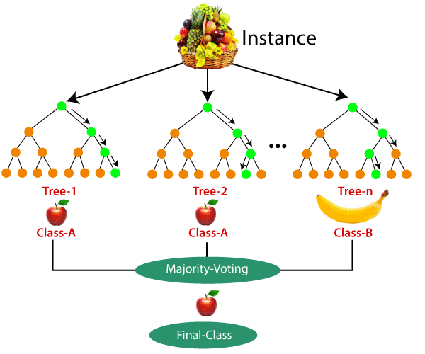
24 |
25 | ### STOCK PREDICTION USING RANDOM FOREST
26 |
27 | In this tutorial of Random forest from scratch, since it is totally based on a decision tree we aren’t going to cover scratch tutorial. You can go through [decision tree from scratch](https://github.com/ghimiresunil/Implementation-of-Machine-Learning-Algorithm-from-Scratch/tree/main/ML%20from%20Scratch/Decision%20Tree).
28 |
29 | ```
30 | import matplotlib.pyplot as plt
31 | import numpy as np
32 | import pandas as pd
33 |
34 | # Import the model we are using
35 | from sklearn.ensemble import RandomForestRegressor
36 |
37 | data = pd.read_csv('data.csv')
38 | data.head()
39 | ```
40 |
41 | | | Date| Open | High| Low| Close| Volume | Name|
42 | | --- | ----| ----| ---- | ---- | ---- | ----| ---- |
43 | | 0 | 2006-01-03| 211.47 | 218.05 | 209.32 | 217.83 | 13137450 | GOOGL|
44 | | 1 | 2006-01-04| 222.17 | 224.70 | 220.09 | 222.84 | 15292353 | GOOGL|
45 | | 2 | 2006-01-05| 223.22 | 226.70 | 220.97 | 225.85 | 10815661a | GOOGL|
46 | | 3 | 2006-01-06| 228.66 | 235.49 | 226.85 | 233.06 | 17759521 | GOOGL|
47 | | 4 | 2006-01-09| 233.44 | 236.94 | 230.70 | 233.68 | 12795837 | GOOGL|
48 |
49 | Here, we will be using the dataset (available below) which contains seven columns namely date, open, high, low, close, volume, and name of the company. Here in this case google is the only company we have used. Open refers to the time at which people can begin trading on a particular exchange. Low represents a lower price point for a stock or index. High refers to a market milestone in which a stock or index reaches a greater price point than previously for a particular time period. Close simply refers to the time at which a stock exchange closes to trading. Volume refers to the number of shares of stock traded during a particular time period, normally measured in average daily trading volume.
50 |
51 | ```
52 | abc=[]
53 | for i in range(len(data)):
54 | abc.append(data['Date'][i].split('-'))
55 | data['Date'][i] = ''.join(abc[i])
56 | ```
57 | Using above dataset, we are now trying to predict the ‘Close’ Value based on all attributes. Let’s split the data into train and test dataset.
58 |
59 | ```
60 | #These are the labels: They describe what the stock price was over a period.
61 | X_1 = data.drop('Close',axis=1)
62 | Y_1 = data['Close']
63 |
64 | # Using Skicit-learn to split data into training and testing sets
65 | from sklearn.model_selection import train_test_split
66 |
67 | X_train_1, X_test_1, y_train_1, y_test_1 = train_test_split(X_1, Y_1, test_size=0.33, random_state=42)
68 | ```
69 |
70 | Now, let’s instantiate the model and train the model on training dataset:
71 |
72 | ```
73 | rfg = RandomForestRegressor(n_estimators= 10, random_state=42)
74 | rfg.fit(X_train_1,y_train_1)
75 | ```
76 |
77 | Let’s find out the features on the basis of their importance by calculating numerical feature importances
78 |
79 | ```
80 | # Saving feature names for later use
81 | feature_list = list(X_1.columns)
82 |
83 | # Get numerical feature importances
84 | importances = list(rfg.feature_importances_)
85 |
86 | # List of tuples with variable and importance
87 | feature_importances = [(feature, round(importance, 2)) for feature, importance in zip(feature_list, importances)]
88 |
89 | # Sort the feature importances by most important first
90 | feature_importances = sorted(feature_importances, key = lambda x: x[1], reverse = True)
91 |
92 | # Print out the feature and importances
93 | [print('Variable: {:20} Importance: {}'.format(*pair)) for pair in feature_importances];
94 | ```
95 |
96 |
97 | 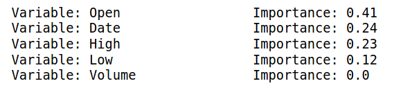
98 |
99 | ```
100 | rfg.score(X_test_1, y_test_1)
101 |
102 | output:- 0.9997798214978976
103 | ```
104 |
105 | We are getting an accuracy of ~99% while predicting. We then display the original value and the predicted Values.
106 |
107 | ```
108 | pd.concat([pd.Series(rfg.predict(X_test_1)), y_test_1.reset_index(drop=True)], axis=1)
109 | ```
110 |
111 | ### ADVANTAGES OF RANDOM FOREST
112 | - It reduces overfitting as it yields prediction based on majority voting.
113 | - Random forest can be used for classification as well as regression.
114 | - It works well on a large range of datasets.
115 | - Random forest provides better accuracy on unseen data and even if some data is missing
116 | - Data normalization isn’t required as it is a rule-based approach
117 |
118 | ### DISADVANTAGES
119 |
120 | - Random forest requires much more computational power and memory space to build numerous decision trees.
121 | - Due to the ensemble of decision trees, it also suffers interpretability and fails to determine the significance of each variable.
122 | - Random forests can be less intuitive for a large collection of decision trees.
123 | - Using bagging techniques, Random forest makes trees only which are dependent on each other. Bagging might provide similar predictions in each tree as the same greedy algorithm is used to create each decision tree. Hence, it is likely to be using the same or very similar split points in each tree which mitigates the variance originally sought.
124 |
--------------------------------------------------------------------------------
/ML from Scratch/Support Vector Machine/README.md:
--------------------------------------------------------------------------------
1 | # Support Vector Machine – SVM From Scratch Python
2 |
3 | 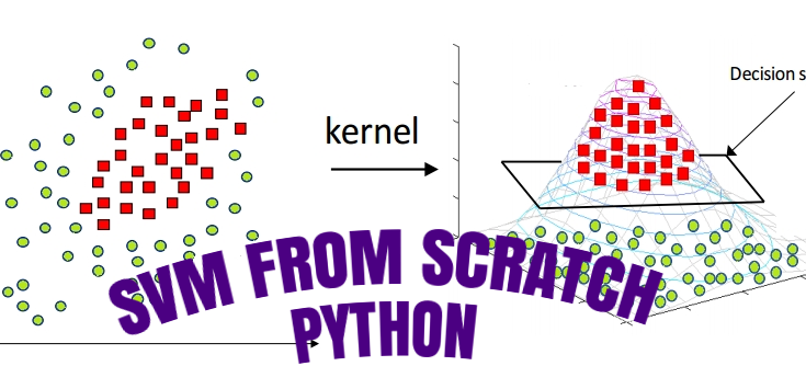
4 |
5 | In the 1960s, Support vector Machine (SVM) known as supervised machine learning classification was first developed, and later refined in the 1990s which has become extremely popular nowadays owing to its extremely efficient results. The SVM is a supervised algorithm is capable of performing classification, regression, and outlier detection. But, it is widely used in classification objectives. SVM is known as a fast and dependable classification algorithm that performs well even on less amount of data. Let’s begin today’s tutorial on SVM from scratch python.
6 |
7 | 
8 |
9 | ## HOW SVM WORKS ?
10 |
11 | SVM finds the best N-dimensional hyperplane in space that classifies the data points into distinct classes. Support Vector Machines uses the concept of ‘Support Vectors‘, which are the closest points to the hyperplane. A hyperplane is constructed in such a way that distance to the nearest element(support vectors) is the largest. The better the gap, the better the classifier works.
12 |
13 |
14 |
15 | The line (in 2 input feature) or plane (in 3 input feature) is known as a decision boundary. Every new data from test data will be classified according to this decision boundary. The equation of the hyperplane in the ‘M’ dimension:
16 |
17 | $y = w_0 + w_1x_1 + w_2x_2 + w_3x_3 + ......= w_0 + \Sigma_{i=1}^mw_ix_i = w_0 + w^{T}X = b + w^{T}X $
18 |
19 | where,
20 | $W_i$ = $vectors\(w_0, w_1, w_2, w_3, ...... w_m\)$
21 |
22 | 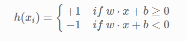
23 |
24 | The point above or on the hyperplane will be classified as class +1, and the point below the hyperplane will be classified as class -1.
25 |
26 | 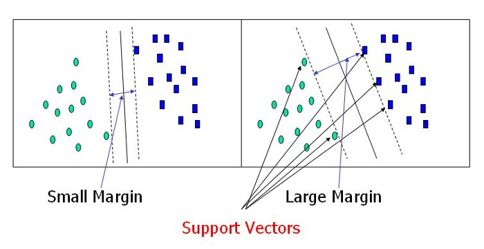
27 |
28 | ## SVM IN NON-LINEAR DATA
29 |
30 | SVM can also conduct non-linear classification.
31 |
32 | 
33 |
34 | For the above dataset, it is obvious that it is not possible to draw a linear margin to divide the data sets. In such cases, we use the kernel concept.
35 |
36 | SVM works on mapping data to higher dimensional feature space so that data points can be categorized even when the data aren’t otherwise linearly separable. SVM finds mapping function to convert 2D input space into 3D output space. In the above condition, we start by adding Y-axis with an idea of moving dataset into higher dimension.. So, we can draw a graph where the y-axis will be the square of data points of the X-axis.
37 |
38 | 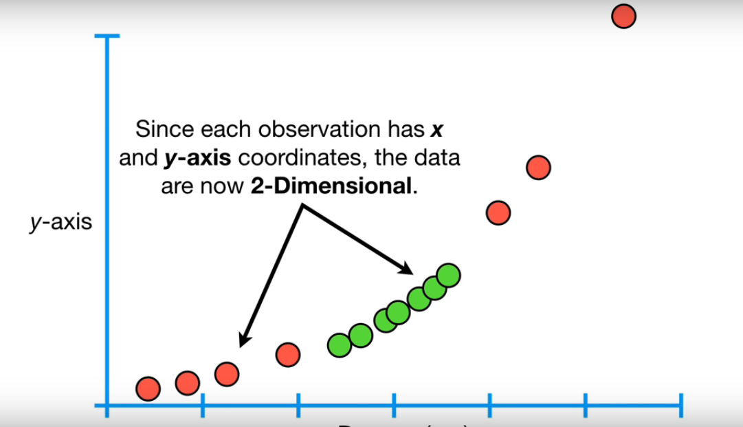
39 |
40 | And now, the data are two dimensional, we can draw a Support Vector Classifier that classifies the dataset into two distinct regions. Now, let’s draw a support vector classifier.
41 |
42 | 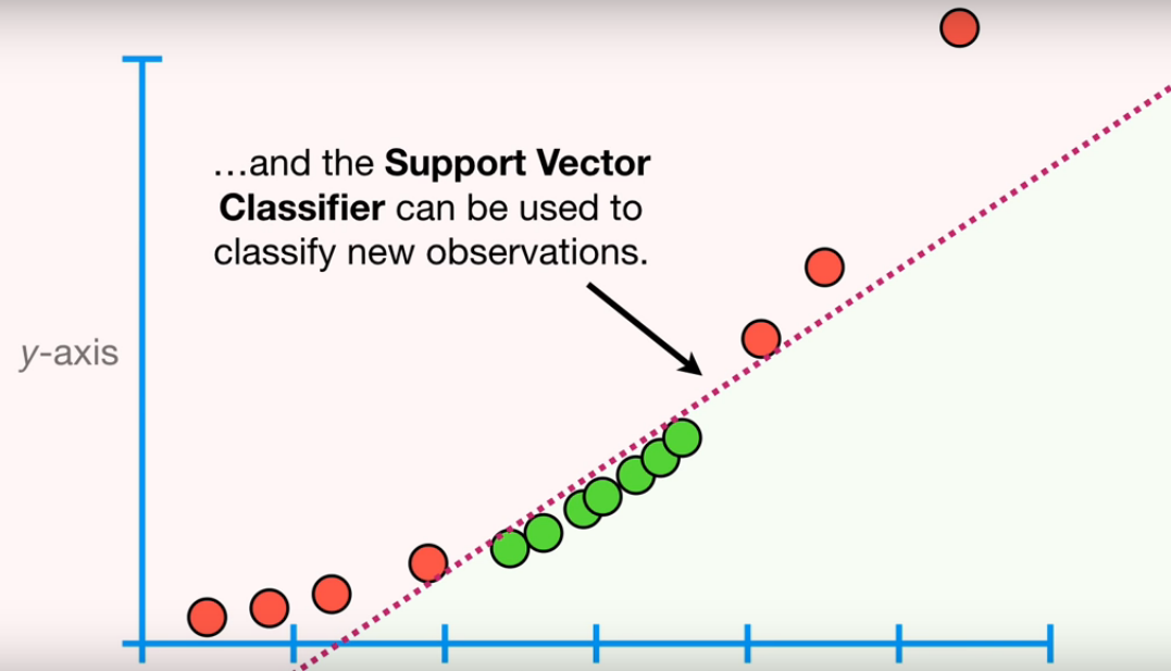
43 |
44 | **_Note_**: This example is taken from [Statquest](https://www.youtube.com/watch?v=efR1C6CvhmE).
45 |
46 | ## HOW TO TRANSFORM DATA ??
47 |
48 | SVM uses a kernel function to draw Support Vector Classifier in a higher dimension. Types of Kernel Functions are :
49 |
50 | - Linear
51 | - Polynomial
52 | - Radial Basis Function(rbf)
53 |
54 | In the above example, we have used a polynomial kernel function which has a parameter d (degree of polynomial). Kernel systematically increases the degree of the polynomial and the relationship between each pair of observation are used to find Support Vector Classifier. We also use cross-validation to find the good value of d.
55 |
56 | ### Radial Basis Function Kernel
57 |
58 | Widely used kernel in SVM, we will be discussing radial basis Function Kernel in this tutorial for SVM from Scratch Python. Radial kernel finds a Support vector Classifier in infinite dimensions. Radial kernel behaves like the Weighted Nearest Neighbour model that means closest observation will have more influence on classifying new data.
59 |
60 | $K(X_1, X_2) = exponent(-\gamma||X_1 - X_2||^2)$
61 |
62 | Where,
63 | $||X_1 - X_2||$ = Euclidean distance between $X_1$ & $X_2$
64 |
65 | ## SOFT MARGIN – SVM
66 | n this method, SVM makes some incorrect classification and tries to balance the tradeoff between finding the line that maximizes the margin and minimizes misclassification. The level of misclassification tolerance is defined as a hyperparameter termed as a penalty- ‘C’.
67 |
68 | For large values of C, the optimization will choose a smaller-margin hyperplane if that hyperplane does a better job of getting all the training points classified correctly. Conversely, a very small value of C will cause the optimizer to look for a larger-margin separating hyperplane, even if that hyperplane misclassifies more points. For very tiny values of C, you should get misclassified examples, often even if your training data is linearly separable.
69 |
70 | Due to the presence of some outliers, the hyperplane can’t classify the data points region correctly. In this case, we use a soft margin & C hyperparameter.
71 |
72 | ## SVM IMPLEMENTATION IN PYTHON
73 | In this tutorial, we will be using to implement our SVM algorithm is the Iris dataset. You can download it from this [link](https://www.kaggle.com/code/jchen2186/machine-learning-with-iris-dataset/data). Since the Iris dataset has three classes. Also, there are four features available for us to use. We will be using only two features, i.e Sepal length, and Sepal Width.
74 |
75 | 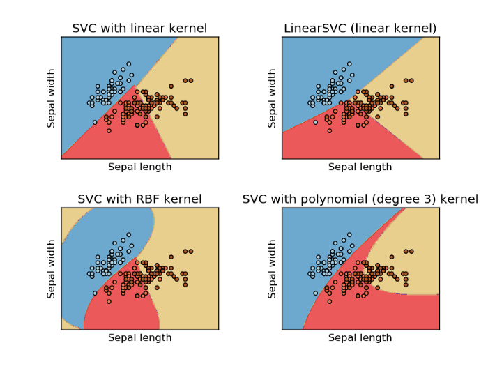
76 |
77 | ## BONUS – SVM FROM SCRATCH PYTHON!!
78 | Kernel Trick: Earlier, we had studied SVM classifying non-linear datasets by increasing the dimension of data. When we map data to a higher dimension, there are chances that we may overfit the model. Kernel trick actually refers to using efficient and less expensive ways to transform data into higher dimensions.
79 |
80 | Kernel function only calculates relationship between every pair of points as if they are in the higher dimensions; they don’t actually do the transformation. This trick , calculating the high dimensional relationships without actually transforming data to the higher dimension, is called the **Kernel Trick**.
81 |
--------------------------------------------------------------------------------
/Machine Learning from Beginner to Advanced/Classification Performance Metrics.md:
--------------------------------------------------------------------------------
1 | # Performance Metrics in Machine Learning Classification Model
2 |
3 | 
4 |
5 | In this file, we are going to talk about 5 of the most widely used Evaluation Metrics of Classification Model. Before going into the details of performance metrics, let’s answer a few points:
6 |
7 | ## WHY DO WE NEED EVALUATION METRICS?
8 |
9 | Being Humans we want to know the efficiency or the performance of any machine or software we come across. For example, if we consider a car we want to know the Mileage, or if we there is a certain algorithm we want to know about the Time and Space Complexity, similarly there must be some or the other way we can measure the efficiency or performance of our Machine Learning Models as well.
10 |
11 | That being said, let’s look at some of the metrics for our Classification Models. Here, there are separate metrics for Regression and Classification models. As Regression gives us continuous values as output and Classification gives us discrete values as output, we will focus on Classification Metrics.
12 |
13 | ### ACCURACY
14 |
15 | The most commonly and widely used metric, for any model, is accuracy, it basically does what It says, calculates what is the prediction accuracy of our model. The formulation is given below:
16 |
17 | Accuracy = $\frac{Number \ of \ correct \ prediction}{Total \ number \ of \ points}\ *\ 100$
18 |
19 | As we can see, it basically tells us among all the points how many of them are correctly predicted.
20 |
21 | **Advantages**
22 | * Easy to use Metric
23 | * Highly Interpretable
24 | * If data points are balanced it gives proper effectiveness of the model
25 |
26 | **Disadvantages**
27 | * Not recommended for Imbalanced data, as results can be misleading. Let me give you an exatample. Let’s say we have 100 data points among which 95 points are negative and 5 points are positive. If I have a dumb model, which only predicts negative results then at the end of training I will have a model that will only predict negative. But still, be 95% accurate based on the above formula. Hence not recommended for imbalanced data.
28 | * We don’t understand where our model is making mistakes.
29 |
30 | ### CONFUSION METRICS
31 |
32 | As the name suggests it is a 2×2 matrix that has Actual and Predicted as Rows and Columns respectively. It determines the number of Correct and Incorrect Predictions, we didn’t bother about incorrect prediction in the Accuracy method, and we only consider the correct ones, so the Confusion Matrix helps us understand both aspects.
33 |
34 | Let’s have a look at the diagram to have a better understanding of it:
35 |
36 | 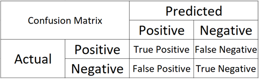
37 |
38 | ### WHAT DOES THESE NOTATION MEANS?
39 |
40 | Imagine I have a binary classification problem with classes as positive and negative labels, now, If my actual point is Positive and my Model predicted point is also positive then I get a True Positive, here “True” means correctly classified and “Positive” is the predicted class by the model, Similarly If I have actual class as Negative and I predicted it as Positive, i.e. an incorrect predicted, then I get False Positive, “False” means Incorrect prediction, and “Positive” is the predicted class by the model.
41 |
42 | We always want diagonal elements to have high values. As they are correct predictions, i.e. TP & TN.
43 |
44 | **Advantages**:
45 | * It specifies a model is confused between which class labels.
46 | * You get the types of errors made by the model, especially Type I or Type II.
47 | * Better than accuracy as it shows the incorrect predictions as well, you understand in-depth the errors made by the model, and rectify the areas where it is going incorrect.
48 |
49 | **Disadvantage**:
50 | * Not very much well suited for Multi-class
51 |
52 | **PRECISION & RECALL**
53 | Precision is the measure which states, among all the predicted positive class, how many are actually positive, formula is given below:
54 |
55 | Precision = $\frac{True Positive}{True Positive + False Positive}$
56 |
57 | Recall is the measure which states, among all the Positive classes how many are actually predicted correctly, formula is given below:
58 |
59 | Recall = $\frac{True Positive}{True Positive + False Negative}$
60 |
61 | We often seek for getting high precision and recall. If both are high means our model is sensible. Here, we also take into consideration, the incorrect points, hence we are aware where our model is making mistakes, and Minority class is also taken into consideration.
62 |
63 | **Advantages**:
64 | * It tells us about the efficiency of the model
65 | * Also shows us how much or data is biased towards one class.
66 | * Helps us understand whether our model is performing well in an imbalanced dataset for the minority class.
67 |
68 | **Disadvantage**
69 | * Recall deals with true positives and false negatives and precision deals with true positives and false positives. It doesn’t deal with all the cells of the confusion matrix. True negatives are never taken into account.
70 | * Hence, precision and recall should only be used in situations, where the correct identification of the negative class does not play a role.
71 | * Focuses only on Positive class.
72 | * Best suited for Binary Classification.
73 |
74 | ### F1-SCORE
75 | F1 score is the harmonic mean of the precision and recall, where an F1 score reaches its best value at 1 (perfect precision and recall). The F1 score is also known as the Sorensen–Dice coefficient or Dice similarity coefficient (DSC).
76 |
77 | It leverages both the advantages of Precision and Recall. An Ideal model will have precision and recall as 1 hence F1 score will also be 1.
78 |
79 | F1 - Score = $2 * \frac{Precision * Recall}{Precision + Recall}$
80 |
81 | **Advantages and Disadvantages**:
82 | * It is as same as Precision and Recall.
83 |
84 | **AU-ROC**
85 |
86 | AU-ROC is the Area Under the Receiver Operating Curve, which is a graph showing the performance of a model, for all the values considered as a threshold. As AU-ROC is a graph it has its own X-axis and Y-axis, whereas X-axis is FPR and Y-axis is TPR
87 |
88 | TPR = $\frac{True Positive}{True Positive + False Negative}$
89 | FPR = $\frac{False Positive}{False Positive + True Negative}$
90 |
91 | ROC curve plots are basically TPR vs. FPR calculated at different classification thresholds. Lowering the classification threshold classifies more items as positive, thus increasing both False Positives and True Positives i.e. basically correct predictions.
92 |
93 | All the values are sorted and plotted in a graph, and the area under the ROC curve is the actual performance of the model at different thresholds.
94 |
95 |
96 |
97 |
98 |
99 | **Advantages**:
100 | * A simple graphical representation of the diagnostic accuracy of a test: the closer the apex of the curve toward the upper left corner, the greater the discriminatory ability of the test.
101 | * Also, allows a more complex (and more exact) measure of the accuracy of a test, which is the AUC.
102 | * The AUC in turn can be used as a simple numeric rating of diagnostic test accuracy, which simplifies comparison between diagnostic tests.
103 |
104 | **Disadvantages**:
105 | * Actual decision thresholds are usually not displayed in the plot.
106 | * As the sample size decreases, the plot becomes more jagged.
107 | * Not easily interpretable from a business perspective.
108 |
109 | _**So there you have it, some of the widely used performance metrics for Classification Models.**_
110 |
--------------------------------------------------------------------------------
/Installation/install_anaconda_python.md:
--------------------------------------------------------------------------------
1 | # How To Install the Anaconda Python on Windows and Linux (Ubuntu and it's Derivatives)
2 |
3 | Setting up software requirements (environment) is the first and the most important step in getting started with Machine Learning. It takes a lot of effort to get all of those things ready at times. When we finish preparing for the work environment, we will be halfway there.
4 |
5 | In this file, you’ll learn how to use Anaconda to build up a Python machine learning development environment. These instructions are suitable for both Windows and Linux systems.
6 |
7 | * Steps are to install Anaconda in Windows & Ubuntu
8 | * Creating & Working On Conda Environment
9 | * Walkthrough on ML Project
10 |
11 | ## 1. Introduction
12 | Anaconda is an open-source package manager, environment manager, and distribution of the Python and R programming languages. It is used for data science, machine learning, large-scale data processing, scientific computing, and predictive analytics.
13 |
14 | Anaconda aims to simplify package management and deployment. The distribution includes 250 open-source data packages, with over 7,500 more available via the Anaconda repositories suitable for Windows,Linux and MacOS. It also includes the conda command-line tool and a desktop GUI called Anaconda Navigator.
15 |
16 | ### 1.1. Install Anaconda on Windows
17 |
18 | * Go to anaconda official website
19 | * [Download](https://www.anaconda.com/products/distribution) based on your Operating set up (64x or 32x) for windows
20 | * After Anaconda has finished downloading, double-click the _.exe_ file to start the installation process.
21 | * Then, until the installation of Windows is complete, follow the on-screen instructions.
22 | * Don’t forget to add the path to the environmental variable. The benefit is that you can use Anaconda in your Command Prompt, Git Bash, cmder, and so on.
23 | * If you like, you can install Microsoft [VSCode](https://code.visualstudio.com/), but it’s not required.
24 | * Click on Finish
25 | * Open a Command Prompt. If the conda is successfully installed then run conda -V or conda –version in the command prompt and it will pop out the installed version.
26 |
27 | ### 1.2. Install Anaconda on Ubuntu and it's derivatives
28 |
29 | ```Anaconda3-2022.05-Linux-x86_64.sh``` is the most recent stable version at the time of writing this post. Check the [Downloads page](https://www.anaconda.com/distribution/) to see whether there is a new version of Anaconda for Python 3 available for download before downloading the installation script.
30 |
31 | Downloading the newest Anaconda installer bash script, verifying it, and then running it is the best approach to install Anaconda. To install Anaconda on Ubuntu, follow the steps below:
32 |
33 | #### Step 01
34 |
35 | Install the following packages if you’re installing Anaconda on a desktop system and want to use the GUI application.
36 |
37 | ```
38 | $ sudo apt install libgl1-mesa-glx libegl1-mesa libxrandr2 libxrandr2 libxss1 libxcursor1 libxcomposite1 libasound2 libxi6 libxtst6
39 | ```
40 |
41 | #### Step 02
42 |
43 | Download the Anaconda installation script with wget
44 |
45 | ```
46 | $ wget -P /tmp https://repo.anaconda.com/archive/Anaconda3-2022.05-Linux-x86_64.sh
47 | ```
48 |
49 | **_Note_**: If you want to work with different version of anaconda, adjust the [version of anaconda](https://repo.anaconda.com/archive/).
50 |
51 | #### Step 03
52 |
53 | For verifying the data integrity of the installer with cryptographic hash verification you can use the ```SHA-256``` checksum. You’ll use the sha256sum command along with the filename of the script:
54 |
55 | ```
56 | $ sha256sum /tmp/Anaconda3-2022.05-Linux-x86_64.sh`
57 | ```
58 |
59 | You’ll receive output that looks similar to this:
60 |
61 | ```
62 | Output:
63 | afcd2340039557f7b5e8a8a86affa9ddhsdg887jdfifji988686bds
64 | ```
65 |
66 | #### Step 04
67 |
68 | To begin the installation procedure, run the script
69 |
70 | ```
71 | $ bash /tmp/Anaconda3-2022.05-Linux-x86_64.sh
72 | ```
73 |
74 | You’ll receive a welcome mesage as output. Press `ENTER` to continue and then press `ENTER` to read through the license. Once you complete reading the license, you will be asked for approving the license terms.
75 |
76 | ```
77 | Output
78 | Do you approve the license terms? [yes|no]
79 | ```
80 |
81 | Type `yes`.
82 |
83 | Next, you’ll be asked to choose the location of the installation. You can press `ENTER` to accept the default location, or specify a different location to modify it.
84 |
85 | Once you are done you will get a thank you message.
86 |
87 | #### Step 05
88 |
89 | Enter the following bash command to activate the Anaconda installation.
90 |
91 | ```
92 | $ source ~/.bashrc
93 | ```
94 |
95 | Once you have done that, you’ll be placed into the default `base` programming environment of Anaconda, and your command prompt will will show base environment.
96 |
97 | ```
98 | $(base) linus@ubuntu
99 | ```
100 |
101 | ### 1.3. Updating Anaconda
102 |
103 | To update the anaconda to the latest version, open and enter the following command:
104 |
105 | ```
106 | (base) linus@ubuntu:~$ conda update --all -y
107 | ```
108 |
109 | ### 1.4. Creating & Working on Conda Environment
110 |
111 | Anaconda virtual environments let us specify specific package versions. You can specify which version of Python to use for each Anaconda environment you create.
112 |
113 | _**Note**_: Name the environment ```venv_first_env``` or some nice and relevant name as per your project.
114 |
115 | ```
116 | (base) linus@ubuntu:~$ conda create --name venv_first_env python=3.9
117 | ```
118 |
119 | You’ll receive output with information about what is downloaded and which packages will be installed, and then be prompted to proceed with `y` or `n`. As long as you agree, type `y`.
120 |
121 | The `conda` utility will now fetch the packages for the environment and let you know when it’s complete.
122 |
123 | You can activate your new environment by typing the following:
124 |
125 | ```
126 | (base) linus@ubuntu:~$ conda activate venv_first_env
127 | ```
128 |
129 | With your environment activated, your command prompt prefix will reflect that you are no longer in the `base` environment, but in the new one that you just created.
130 |
131 | When you’re ready to deactivate your Anaconda environment, you can do so by typing:
132 |
133 | ```
134 | (venv_first_env) linus@ubuntu:~$ conda deactivate
135 | ```
136 |
137 | With this command, you can see the list of all of the environments you’ve created:
138 |
139 | ```
140 | (base) linus@ubuntu:~$ conda info --envs
141 | ```
142 |
143 | When you create environment using `conda create` , it will come with several default packages. Few examples of then are:
144 |
145 |
146 | - `openssl`
147 | - `pip`
148 | - `python`
149 | - `readline`
150 | - `setuptools`
151 | - `sqlite`
152 | - `tk`
153 |
154 | You might need to add additional package in your environment .
155 |
156 | You can add packages such as `matplotlib` for example, with the following command:
157 |
158 | ```
159 | (venv_first_env) linus@ubuntu:~$ conda install matplotlib
160 | ```
161 |
162 |
163 | For installing the specific version, you can specify specific version with the following command:
164 | ```
165 | (venv_first_env) linus@ubuntu:~$ conda install matplotlib=1.4.3
166 | ```
167 |
168 |
169 | ### 1.5. Getting Started With Jupyter Notebook
170 |
171 | Jupyter Notebooks are capable of performing data visualization in the same environment and are strong, versatile, and shared. Data scientists may use Jupyter Notebooks to generate and distribute documents ranging from code to full-fledged reports.
172 |
173 | You can directly launch Juypter through the terminal using the following command:
174 |
175 | #### Command 01:
176 | ```
177 | (venv_first_env) linus@ubuntu:~$ jupyter notebook
178 | ```
179 |
180 | #### command 02:
181 | ```
182 | (venv_first_env) linus@ubuntu:~$ jupyter notebook --no-browser --port=8885
183 | ```
184 |
185 | ### 06. Working with Jupyter Noteboook
186 |
187 | * create a new notebook, click on the New button on the top right hand corner of the web page and select `Python 3 notebook`. The Python statements are entered in each cell. To execute the Python statements within each cell, press both the `SHIFT` and `ENTER` keys simultaneously. The result will be displayed right below the cell.
188 | * By default, the new notebook will be stored in a file named `Untitled.ipynb`. You can rename the file by clicking on File and Rename menu option at the top
189 | * You can save the notebook by clicking on the `'File'` and `'Save and Checkpoint'` menu options. The notebook will be stored in a file with a `'.ipynb'` extension. You can open the notebook and re-run the program and the results you have saved any time. This powerful feature allows you to share your program and results as well as to reproduce the results generated by others. You can also save the notebook into an HTML format by clicking 'File' followed by 'Download as' options. Note that the IPython notebook is not stored as standard ASCII text files; instead, it is stored in Javascript Object Notation (JSON) file format.
190 |
191 |
🙂 Now we are all done with being ready for Machine learning 🙂
192 |
193 |
--------------------------------------------------------------------------------
/Mathematical Implementation/confusion_matrix.md:
--------------------------------------------------------------------------------
1 | # CONFUSION MATRIX FOR YOUR MULTI-CLASS ML MODEL
2 |
3 | Many multi-class and multi-label categorization difficulties in daily life. In contrast to multi-class classification issues, multi-label classification problems may have an array of classes as the result, but in multi-class classification problems there is only one output out of several targets. An apple, for instance, is red, healthy, and sweet. A stackoverflow topic may also be labeled with Python, Machine Learning, or Data Science. The multi-label classification problem is quickly shown in the following graphic.
4 |
5 | 
6 |
7 | For the sake of simplicity, let’s assume our multi-class classification problem to be a 3-class classification problem. Say we have got three class labels(Target/Outcome) in a dataset, namely 0, 1, and 2. A potential uncertainty matrix for these groups is provided below.
8 |
9 | 
10 |
11 | Unlike binary classification, there are no positive or negative classes here. At first, it might be a little difficult to find TP, TN, FP, and FN since there are no positive or negative classes, but it’s actually pretty easy
12 |
13 | ## 1. Accuracy
14 |
15 | Accuracy is the most commonly used matrix to evaluate the model which is actually not a clear indicator of the performance.
16 |
17 | Accuracy = $\frac{34 + 52 + 33}{150} = 0.793$
18 |
19 | ## 2. Misclassification Rate/ Error
20 |
21 | Error tells you what fraction of predictions were incorrect. It is also known as Classification Error.
22 |
23 | Misclassification Rate/ Error = 1 - Accuracy = 1 - 0.793 = 0.207
24 |
25 | ## 3. Precision / Positive Predicted Value
26 |
27 | Precision is the percentage of positive instances out of the total predicted positive instances which means precision or positive predicted value means how much model is right when it says it is right.
28 |
29 | * Precision for Class 0 = $\frac{34}{34 + 0 + 13} = 0.723$
30 |
31 | * Precision for Class 1 = $\frac{52}{13 + 52 + 0} = 0.8$
32 |
33 | * Precision for Class 2 = $\frac{33}{5 + 0 + 33} = 0.868$
34 |
35 | ## 4. Recall / True Positive Rate / Sensitivity
36 |
37 | Recall literally is how many of the true positives were recalled (found), i.e. how many of the correct hits were also found.
38 |
39 | * Recall for Class 0 = $\frac{34}{34 + 13 + 5} = 0.653$
40 |
41 | * Recall for Class 1 = $\frac{52}{0 + 52 + 0} = 1$
42 |
43 | * Recall for class 2 = $\frac{33}{13 + 0 + 33} = 0.7173$
44 |
45 | ## 5. F1-Score
46 |
47 | Before we dive deep into F1 score, the question may arise in your mind about what is F Score?
48 |
49 | The F-measure balances the precision and recall.
50 |
51 | On some problems, when false positives are more essential to minimize than false negatives, we could be interested in an F-measure that places greater emphasis on Precision.
52 |
53 | On other problems, when false negatives are more essential to minimize than false positives, we could be interested in an F-measure that places greater emphasis on Recall.
54 |
55 | The solution is the **Fbeta-measure**.
56 |
57 | Using an abstraction of the F-measure known as the Fbeta-measure, a beta-coefficient is used to balance recall and precision when calculating the harmonic mean.
58 |
59 | So,
60 |
61 | $F_{\beta} = \frac{1 + \beta^2 * (Precision * Recall)}{\beta^2 * (Precision + Recall)} $
62 |
63 | The choice of the beta parameter will be used in the name of the Fbeta-measure.
64 | For example, a beta value of 2 is referred to as F2-measure or F2-score. A beta value of 1 is referred to as the F1-measure or the F1-score.
65 |
66 | Three common values for the beta parameter are as follows:
67 |
68 | * **F0.5-Measure** (beta=0.5): More weight on precision, less weight on recall.
69 | * **F1-Measure** (beta=1.0): Balance the weight on precision and recall.
70 | * **F2-Measure** (beta=2.0): Less weight on precision, more weight on recall
71 |
72 | The F-measure discussed in the previous section is an example of the Fbeta-measure with a beta value of 1.
73 |
74 | F1- Score is the harmonic mean of the precision and recall which means the higher the value of the f1-score better will be the model. Due to the product in the numerator, if one goes low, the final F1 score goes down significantly. So a model does well in F1 score if the positive predicted are actually positives (precision) and doesn't miss out on positives and predicts them negative (recall).
75 |
76 | * F1- Score of Class 0 = $\frac{2 \times R_0 \times P_0}{R_0 + P_0} = \frac{2 \times 0.723 \times 0.653}{0.7223 + 0.6563} = 0.6886$
77 |
78 | * F1- Score of Class 1 = $\frac{2 \times R_1 \times P_1}{R_1 + P_1} = \frac{2 \times 0.8 \times 1}{0.8 + 1} = 0.8888$
79 |
80 | * F1- Score of Class 2 = $\frac{2 \times R_2 \times P_2}{R_2 + P_2} = \frac{2 \times 0.868 \times 0.7170}{0.868 + 0.7170} = 0.785$
81 |
82 | ## 6. Support
83 |
84 | The support is the number of occurrences of each particular class in the true responses (responses in your test set). Support can calculate by summing the rows of the confusion matrix.
85 |
86 | Here, the support for classes 0, 1, and 2 is 52, 52, and 46.
87 |
88 | * Support for Class 0 = 52
89 | * Support for Class 1 = 52
90 | * Support for Class 2 = 46
91 |
92 | ## 7. Micro F1
93 |
94 | This is called a micro-averaged F1-score. It is calculated by considering the total TP, total FP and total FN of the model. It does not consider each class individually, It calculates the metrics globally. So for our example,
95 |
96 | * Total TP = 34 + 52 + 33 = 119
97 | * Total FP = (0 + 13) + (13 + 0) + (5 + 0) = 31
98 | * Total FN = (13 + 5) + (0 + 0) + (13+0) = 31
99 |
100 | Hence,
101 |
102 | * $Micro_{Recall} = \frac{TP}{TP + FN} = \frac{119}{119 + 31} = 0.793 $
103 |
104 | * $Micro_{Precision} = \frac{TP}{TP + FP} = \frac{119}{119 + 31} = 0.793 $
105 |
106 | Now we can use the regular formula for F1-score and get the Micro F1-score using the above precision and recall.
107 |
108 | * Micro F1-Score = $\frac{2 \times Micro_{Recall} \times Micro_{Precision}}{ Micro_{Recall} + Micro_{Precision}} = \frac{2 \times 0.793 \times 0.793}{0.793 + 0.793} = 0.793$
109 |
110 | _**As you can see When we are calculating the metrics globally all the measures become equal. Also if you calculate accuracy you will see that,**_
111 |
112 | ```
113 | Precision = Recall = Micro F1 = Accuracy
114 | ```
115 |
116 | ## 8. Macro F1
117 |
118 | This is macro-averaged F1-score. It calculates metrics for each class individually and then takes unweighted mean of the measures. As we have seen “Precision, Recall and F1-score for each Class.
119 |
120 | | Precision | Recall | F1-Score |
121 | | --------- | -------| ---------|
122 | | Class 0 Precision = 0.723 | Class 0 Recall= 0.653 | Class 0 F1-Score = 0.686 |
123 | | Class 1 Precision = 0.8 | Class 1 Recall=1 | Class 1 F1-Score = 0.8888 |
124 | | Class 2 Precision = 0.868 | Class 2 Recall= 0.7173 | Class 2 F1-Score = 0.785 |
125 |
126 |
127 | Hence,
128 |
129 | * Macro Average for Precision = $\frac{0.723 + 0.8 + 0.868}{3} = 0.797$
130 |
131 | * Macro Average for Recall = $\frac{0.653 + 1 + 0.7173}{3} = 0.7901$
132 |
133 | * Macro Average for F1-Score = $\frac{0.686 + 0.8888 + 0.785}{3} = 0.7866$
134 |
135 | ## 9. Weighted Average
136 |
137 | Weighted Average is the method of calculating a kind of arithmetic mean of a set of numbers in which some elements of the set have greater (weight) value than others. Unlike Macro F1, it takes a weighted mean of the measures. The weights for each class are the total number of samples of that class.
138 |
139 | * Weighted Average for precision = $\frac{0.723 \times 47 + 0.8 \times 65 + 0.868 \times 38}{150} = 0.7931$
140 |
141 | * Weighted Average for Recall = $\frac{0.653 \times 52 + 1 \times 52 + 0.7173 \times 46}{150} = 0.79301$
142 |
143 | * Weighted Average for F1-Score = $\frac{2 \times 𝑊𝑒𝑖𝑔ℎ𝑡𝑒𝑑_{𝑅𝑒𝑐𝑎𝑙𝑙} \times 𝑊𝑒𝑖𝑔ℎ𝑡𝑒𝑑_{𝑃𝑟𝑒𝑐𝑖𝑠𝑖𝑜𝑛}}{𝑊𝑒𝑖𝑔ℎ𝑡𝑒𝑑_{𝑅𝑒𝑐𝑎𝑙𝑙} + 𝑊𝑒𝑖𝑔ℎ𝑡𝑒𝑑_{𝑃𝑟𝑒𝑐𝑖𝑠𝑖𝑜𝑛}} = 0.79305 $
144 |
145 | ## 10. Cohen's Kappa
146 |
147 | Cohen's kappa measures the agreement between two raters who each classify N items into C mutually exclusive categories. The definition of
148 |
149 | $ Kappa (\kappa) = \frac{P_o - P_e}{1 - P_e}$
150 |
151 | Where,
152 |
153 | $P_o$ = relative observed agreement among raters
154 |
155 | $P_e$ = hypothetical probability of chance agreement
156 |
157 | so,
158 |
159 | $P_o = \frac{34 + 52 + 33}{150} = 0.793$
160 |
161 | $P_e$ = $[(\frac{52}{150} * \frac{47}{150}) + (\frac{52}{150} * \frac{65}{150}) + (\frac{46}{150} * \frac{38}{150})] = [0.108 + 0.150 + 0.077] = 0.335$
162 |
163 | $Kappa (\kappa) = \frac{P_o - P_e}{1 - P_e} = \frac{0.793 - 0.335}{1 - 0.335} = 0.688$
164 |
165 | **_Note_** = Cohen suggested the Kappa result be interpreted as follows: values ≤ 0 as indicating no agreement and 0.01–0.20 as none to slight, 0.21–0.40 as fair, 0.41– 0.60 as moderate, 0.61–0.80 as substantial, and 0.81–1.00 as almost perfect agreement
166 |
167 | **Finally, let’s look generated Confusion matrix using Python’s Scikit-Learn**
168 | 
169 |
170 |
--------------------------------------------------------------------------------
/ML from Scratch/Decision Tree/README.md:
--------------------------------------------------------------------------------
1 | # DECISION TREE FROM SCRATCH
2 |
3 | 
4 |
5 | ## 1. INTRODUCTION
6 | A decision tree is essentially a series of if-then statements, that, when applied to a record in a data set, results in the classification of that record. Therefore, once you’ve created your decision tree, you will be able to run a data set through the program and get a classification for each individual record within the data set. What this means to you, as a manufacturer of quality widgets, is that the program you create from this article will be able to predict the likelihood of each user, within a data set, purchasing your finely crafted product.
7 |
8 | A decision tree is a type of supervised learning algorithm (having a pre-defined target variable) that is mostly used in classification problems. It works for both categorical and continuous input and output variables. In this technique, we split the population or sample into two or more homogeneous sets (or sub-populations) based on the most significant splitter/differentiator in input variables.
9 |
10 | ## 1.1. HOW DECISION TREE WORKS ??
11 | The understanding level of the Decision Trees algorithm is so easy compared with other classification algorithms. The decision tree algorithm tries to solve the problem, by using tree representation. Each internal node of the tree corresponds to an attribute, and each leaf node corresponds to a class label.
12 |
13 | ## 1.2. DECISION TREE ALGORITHM PSEUDOCODE
14 | * Place the best attribute of the dataset at the root of the tree.
15 | * Split the training set into subsets. Subsets should be made in such a way that each subset contains data with the same value for an attribute.
16 | * Repeat step 1 and step 2 on each subset until you find leaf nodes in all the branches of the tree.
17 |
18 | ## 1.3. DECISION TREE CLASSIFIER
19 | In decision trees, for predicting a class label for a record we start from the root of the tree. We compare the values of the root attribute with the record’s attribute. On the basis of comparison, we follow the branch corresponding to that value and jump to the next node.
20 |
21 | We continue comparing our record’s attribute values with other internal nodes of the tree until we reach a leaf node with predicted class value. As we know how the modeled decision tree can be used to predict the target class or the value. Now let’s understand how we can create the decision tree model.
22 |
23 | ## 1.4. ASSUMPTIONS WHILE CREATING DECISION TREE
24 | The below are the some of the assumptions we make while using Decision tree:
25 | * In the beginning, the whole training set is considered as the root.
26 | * Feature values are preferred to be categorical. If the values are continuous then they are discredited prior to building the model.
27 | * Records are distributed recursively on the basis of attribute values.
28 | * Order to placing attributes as root or internal node of the tree is done by using some statistical approach.
29 |
30 | ## 1.5. HOW TO SPLIT NODES ?
31 | There are a few algorithms to find an optimum split. Let’s look at the following to understand the mathematics behind.
32 |
33 | ### 1.5.1. ENTROPY
34 | An alternative splitting criterion for decision tree learning algorithms is information gain. It measures how well a particular attribute distinguishes among different target classifications. Information gain is measured in terms of the expected reduction in the entropy or impurity of the data. The entropy of a set of probabilities is:
35 |
36 | Entropy = $\Sigma_{i = 1}^{c}-p_i*log_{2}(p_i)$
37 |
38 | If we have a set of binary responses from some variable, all of which are positive/true/1, then knowing the values of the variable does not hold any predictive value for us, since all the outcomes are positive. Hence, the entropy is zero
39 |
40 | The entropy calculation tells us how much additional information we would obtain with knowledge of the variable.
41 |
42 | So, if we have a set of candidate covariates from which to choose as a node in a decision tree, we should choose the one that gives us the most information about the response variable (i.e. the one with the highest entropy).
43 |
44 | ### 1.5.2. GINI INDEX
45 | The Gini index is simply the expected error rate:
46 |
47 | Gini = $1 - \Sigma_{i=1}^{c}(p_i)^2$
48 |
49 | ### 1.5.3. ID3
50 | A given cost function can be used to construct a decision tree via one of several algorithms. The Iterative Dichotomies 3 (ID3) is on such an algorithm, which uses entropy, and a related concept, information gain, to choose features and partitions at each classification step in the tree.
51 |
52 | Information gain is the difference between the current entropy of a system and the entropy measured after a feature is chosen.
53 |
54 | Gain(T, X) = Entropy(T) - Entropy(T, X)
55 |
56 | 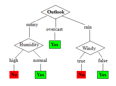
57 |
58 | Note: See dteils about [Here](https://sefiks.com/2017/11/20/a-step-by-step-id3-decision-tree-example/)
59 |
60 | ## 1.6. DECISION TREE USING SKLEARN
61 | To proceed, you need to import all the required libraries that we require in our further coding. Here we have imported graphviz to visualize decision tree diagram. This is can install in conda environment using conda install python-graphviz .
62 |
63 | ```
64 | import numpy as np
65 | import pandas as pd
66 | from sklearn.tree import export_graphviz
67 | import IPython, graphviz, re
68 | RANDOM_SEED = 42
69 |
70 | np.random.seed(RANDOM_SEED)
71 | ```
72 |
73 | We’re going to use the iris dataset. The task for us is now to find the best “way” to split the dataset such that best nodes can be achieved.
74 |
75 | ```
76 | df = pd.read_csv("iris.csv")
77 |
78 | df['species_label'],_ = pd.factorize(df['species'])
79 | y = df['species_label']
80 | X = df[['petal_length', 'petal_width']]
81 | ```
82 |
83 | Now let’s define a class which draws a representation of a random forest in IPython.
84 |
85 | ```
86 | def draw_tree(t, df, size=10, ratio=0.6, precision=0):
87 | s=export_graphviz(t, out_file=None, feature_names=df.columns, filled=True,
88 | special_characters=True, rotate=True, precision=precision)
89 | IPython.display.display(graphviz.Source(re.sub('Tree {',
90 | f'Tree {{ size={size}; ratio={ratio}', s)))
91 | ```
92 |
93 | We are using RandomForestRegressor with 1 estimator, which basically means we’re using a Decision Tree model. Here is the tree structure of our model:
94 |
95 | ```
96 | from sklearn.ensemble import RandomForestRegressor
97 |
98 | reg = RandomForestRegressor(n_estimators=1, max_depth=2, bootstrap=False, random_state=RANDOM_SEED)
99 | reg.fit(X, y)
100 |
101 | draw_tree(reg.estimators_[0], X, precision=2)
102 | ```
103 |
104 | 
105 |
106 | Decision tree models can be used for both classification and regression. The algorithms for building trees break down a data set into smaller and smaller subsets while at the same time an associated decision tree is incrementally developed. The final result is a tree with decision nodes and leaf nodes. A decision node has two or more branches. Leaf node represents a classification or decision (used for regression). The topmost decision node in a tree that corresponds to the best predictor (most important feature) is called a root node. Decision trees can handle both categorical and numerical data.
107 |
108 | ```
109 | X_train,X_test,y_train,y_test = model_selection.train_test_split(X, y, test_size=0.3, random_state=1)
110 |
111 | dtree = tree.DecisionTreeClassifier(criterion='entropy' , max_depth=3, random_state = 0)
112 |
113 | dtree.fit(X_train, y_train)
114 | ```
115 |
116 | Finally, let’s look at how we use all this to make predictions.
117 | ```
118 | y_pred = dtree.predict(X_test)
119 |
120 | count_misclassified = (y_test != y_pred).sum()
121 | print('Misclassified samples: {}'.format(count_misclassified))
122 |
123 | accuracy = metrics.accuracy_score(y_test, y_pred)
124 | print('Accuracy: {:.2f}'.format(accuracy))
125 |
126 | Output:
127 | Misclassified samples: 2
128 | Accuracy: 0.96
129 | ```
130 |
131 | ## 1.7. CROSS-VALIDATION
132 | Cross-Validation is a technique that involves reserving a particular sample of a data set on which you do not train the model. Later, you test the model on this sample before finalizing the model.
133 |
134 | Here are the steps involved in cross-validation:
135 |
136 | * You reserve a sample data set.
137 | * Train the model using the remaining part of the data set.
138 | * Use the reserve sample of the data set test (validation) set. This will help you to know the effectiveness of model performance. If your model delivers a positive result on validation data, go ahead with the current model. It rocks!
139 |
140 | ## 1.8. OVERFITTING
141 |
142 | Overfitting is a practical problem while building a decision tree model. The model is having an issue of overfitting is considered when the algorithm continues to go deeper and deeper in the to reduce the training set error but results with an increased test set error i.e, Accuracy of prediction for our model goes down. It generally happens when it builds many branches due to outliers and irregularities in data.
143 |
144 | Two approaches which we can use to avoid overfitting are:
145 |
146 | * **Pre-Pruning**: In pre-pruning, it stops the tree construction bit early. It is preferred not to split a node if its goodness measure is below a threshold value. But it’s difficult to choose an appropriate stopping point.
147 |
148 | * **Post-Pruning**: In post-pruning first, it goes deeper and deeper in the tree to build a complete tree. If the tree shows the overfitting problem then pruning is done as a post-pruning step. We use a cross-validation data to check the effect of our pruning. Using cross-validation data, it tests whether expanding a node will make an improvement or not.
If it shows an improvement, then we can continue by expanding that node. But if it shows a reduction in accuracy then it should not be expanded i.e, the node should be converted to a leaf node.
149 |
150 | ## 1.9. DECISION TREE ALGORITHM ADVANTAGES AND DISADVANTAGES
151 |
152 | ### 1.9.1. ADVANTAGES
153 | * Decision Trees are easy to explain. It results in a set of rules.
154 | * It follows the same approach as humans generally follow while making decisions.
155 | * The interpretation of a complex Decision Tree model can be simplified by its visualizations. Even a naive person can understand logic.
156 | * The Number of hyper-parameters to be tuned is almost null.
157 |
158 | ### 1.9.2. DISADVANTAGES
159 | * There is a high probability of overfitting in the Decision Tree.
160 | * Generally, it gives low prediction accuracy for a dataset as compared to other machine learning algorithms.
161 | * Information gain in a decision tree with categorical variables gives a biased response for attributes with greater no. of categories.
162 | * Calculations can become complex when there are many class labels.
163 |
--------------------------------------------------------------------------------
/ML from Scratch/KNN/README.md:
--------------------------------------------------------------------------------
1 | # KNN FROM SCRATCH – MACHINE LEARNING FROM SCRATCH
2 |
3 | K nearest neighbors or KNN algorithm is non-parametric, lazy learning, supervised algorithm used for classification as well as regression. KNN is often used when searching for similar items, such as finding items similar to this one. The Algorithm suggests that you are one of them because you are close to your neighbors. Now, let’s begin the article ” KNN from Scratch“.
4 |
5 | ## How does a KNN algorithm work?
6 |
7 | To conduct grouping, the KNN algorithm uses a very basic method to perform classification. When a new example is tested, it searches at the training data and seeks the k training examples which are similar to the new test example. It then assigns to the test example of the most similar class label.
8 |
9 | ### WHAT DOES ‘K’ IN THE KNN ALGORITHM REPRESENT?
10 |
11 | K in KNN algorithm represents the number of nearest neighboring points that vote for a new class of test data. If k = 1, then test examples in the training set will be given the same label as the nearest example. If k = 5 is checked for the labels of the five closest classes and the label is assigned according to the majority of the voting.
12 |
13 | 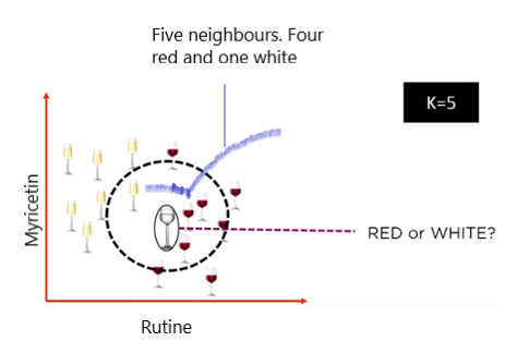
14 |
15 | ### ALGORITHM
16 |
17 | - Initialize the best value of K
18 | - Calculate the distance between test data and trained data using Euclidean distance or any other method
19 | - Check class categories of nearest neighbors and determine the type in which test input falls.
20 | - Classify the test data according to majority vote of nearest K dataset
21 |
22 | ### KNN FROM SCRATCH: MANUAL GUIDE
23 |
24 | Let’s consider an example of height and weight
25 |
26 | The given dataset is about the height and weight of the customer with the respective t-shirt size where M represents the medium size and L represents the large size. Now we need to predict the t-shirt size for the new customer with a height of 169 cm and weight as 69 kg.
27 |
28 | | Height | Weight | T-Shirt Size |
29 | |:------:| :------:| :----------:|
30 | | 150 | 51 | M |
31 | | 158 | 51 | M |
32 | | 158 |53 | M |
33 | | 158 | 55 | M |
34 | | 159 | 55 | M |
35 | | 159 | 56 | M |
36 | | 160 | 57 | M |
37 | | 160 | 58 | M |
38 | | 160 | 58 | M |
39 | | 162 | 52 | L |
40 | | 163 | 53 | L |
41 | | 165 | 53 | L |
42 | | 167 | 55 | L |
43 | | 168 | 62 | L |
44 | | 168 | 65 | L |
45 | | 169 | 67 | L |
46 | | 169 | 68 | L |
47 | | 170 | 68 | L |
48 | | 170 | 69 | L |
49 |
50 | ### CALCULATION
51 |
52 | Note: Predict the t-shirt size of new customer whose name is Sunil with height as 169cm and weight as 69 Kg.
53 |
54 | **Step 1**: The initial step is to calculate the Euclidean distance between the existing points and new points. For example, the existing point is (4,5) and the new point is (1, 1).
55 |
56 | So, P1 = (4,5) where $x_1$ = 4 and $y_1$ = 5
57 | P2 = (1,1) where $x_2$ = 1 and $y_2$ = 1
58 |
59 | 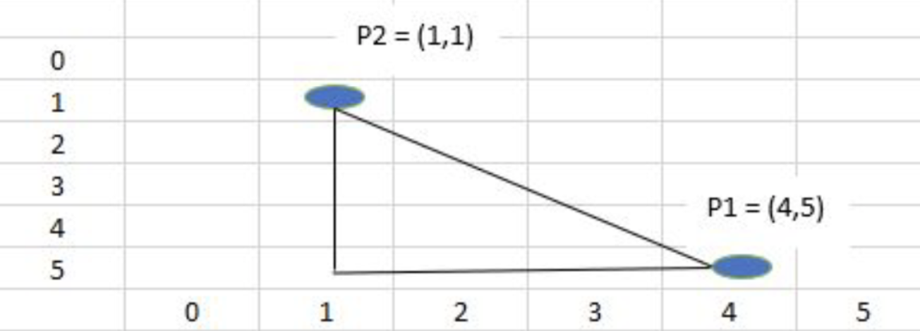
60 |
61 | Now Euclidean distance = $\sqrt{(x_2 - x_1)^2 + (y_2 - y_1)^2}$ = $\sqrt{(1 - 4)^2 + (1 - 5)^2}$ = 5
62 |
63 | **Step 2**: Now, we need to choose the k value and select the closest k neighbors to the new item. So, in our case, **K = 5**, bold elements have the least Euclidean distance as compared with others.
64 |
65 | | Height | Weight | T-Shirt Size | Distance |
66 | | :-----: | :------: | :----------: | :--------|
67 | | 150 | 51 | M | 26.17 |
68 | | 158 | 51 | M | 21.09 |
69 | | 158 | 53 | M | 19.41 |
70 | | 158 | 55 | M | 17.80 |
71 | | 159 | 55 | M | 17.20 |
72 | | 159 | 56 | M | 16.40 |
73 | | 160 | 57 | M | 15 |
74 | | 160 | 58 | M | 14.21 |
75 | | 160 | 58 | M | 14.21 |
76 | | 162 | 52 | L | 18.38 |
77 | | 163 | 53 | L | 16.49 |
78 | | 165 | 53 | L | 16.49 |
79 | | 167 | 55 | L | 14.14 |
80 | | **168** | **62** | **L** | **7.01** |
81 | | **168** | **65** | **L** | **4.12** |
82 | | **169** | **67** | **L** | **2** |
83 | | **169** | **68** | **L** | **2.23** |
84 | | **170** | **68** | **L** | **1.41** |
85 | | 170 | 69 | L | 10.04 |
86 |
87 | **Step 3**: Since, K = 5, we have 5 t-shirts of size L. So a new customer with a height of 169 cm and a weight of 69 kg will fit into t-shirts of L size.
88 |
89 | ### BEST K-VALUE IN KNN FROM SCRATCH
90 |
91 | K in the KNN algorithm refers to the number of nearest data to be taken for the majority of votes in predicting the class of test data. Let’s take an example how value of K matters in KNN.
92 |
93 | 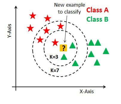
94 |
95 | In the above figure, we can see that if we proceed with K=3, then we predict that test input belongs to class B, and if we continue with K=7, then we predict that test input belongs to class A.
96 |
97 | Data scientists usually choose K as an odd number if the number of classes is 2 and another simple approach to select k is set k=sqrt(n). Similarly, you can choose the minimum value of K, find its prediction accuracy, and keep on increasing the value of K. K value with highest accuracy can be used as K value for rest of the prediction process.
98 |
99 | 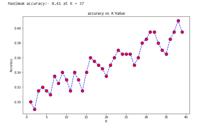
100 |
101 | ### KNN USING SCIKIT-LEARN
102 |
103 | The example below demonstrates KNN implementation on the iris dataset using the scikit-learn library where the iris dataset has petal length, width and sepal length, width with species class/label. Our task is to build a KNN model based on sepal and petal measurements which classify the new species.
104 |
105 | #### STEP 1: IMPORT THE DOWNLOADED DATA AND CHECK ITS FEATURES.
106 |
107 | ```
108 | >>> import pandas as pd
109 | >>> iris = pd.read_csv('../dataset/iris.data', header = None)
110 |
111 | ## attribute to return the column labels of the given Dataframe
112 | >>> iris.columns = ["sepal_length", "sepal_width",
113 | ... "petal_length", "petal_width", "target_class"]
114 | >>> iris.dropna(how ='all', inplace = True)
115 | >>> iris.head()
116 | ```
117 |
118 | | sepal_length | sepal_width | petal_length | petal_width | target_class|
119 | | :-----------: | :-----------: | :-----------: | :-----------: | :-----------: |
120 | | 5.1 | 3.5 | 1.4 | 0.2 | Iris-setosa |
121 | | 4.9 | 3.0 | 1.4 | 0.2| Iris-setosa |
122 | | 4.7 | 3.2 | 1.3 | 0.2 | Iris-setosa |
123 | | 4.6 | 3.1 | 1.5 | 0.2 | Iris-setosa |
124 | | 5.0 | 3.6 | 1.4 | 0.2 | Iris-setosa |
125 |
126 | The **Iris Dataset** contains four features (length and width of sepals and petals) of 50 samples of three **species** of Iris (Iris **setosa**, Iris **virginica**, and Iris **versicolor**). Here, target_class is in a categorical form that can not be handled by machine learning algorithms like KNN. So feature and response should be numeric i.e. NumPy arrays which have a specific shape. For this, we have implemented a LabelEncoder for target_class which are encoded as 0 for iris_setosa, 1 for iris_versicolor, and 2 for iris_verginica.
127 |
128 | #### STEP 2: SPLIT THE DATA INTO TRAIN SET AND TEST SET AND TRAIN THE KNN MODEL
129 |
130 | It is not an optimal approach for training and testing on the same data, so we need to divide the data into two parts, the training set and testing test. For this function called ‘train_test_split’ provided by Sklearn helps to split the data where the parameter like ‘test_size’ split the percentage of train data and test data.
131 |
132 | ‘Random_state’ is another parameter which helps to give the same result every time when we run our model means to split the data, in the same way, every time. As we are training and testing on various datasets, the subsequent quality of the tests should be a stronger approximation of how well the model would do on unknown data.
133 |
134 | ```
135 | ## splitting the data into training and test sets
136 | >>> from sklearn.model_selection import train_test_split
137 | >>> X_train, X_test, y_train, y_test = train_test_split(data, target,
138 | ... test_size = 0.3, random_state = 524)
139 | ```
140 |
141 | #### STEP 3: IMPORT ‘KNEIGHBORSCLASSIFIER’ CLASS FROM SKLEARN
142 |
143 | It is important to select the appropriate value of k, so we use a loop to fit and test the model for various values for K (for 1 – 25) and measure the test accuracy of the KNN. Detail about choosing K is provided in the above KNN from scratch section.
144 |
145 | ```
146 | ## Import ‘KNeighborsClassifier’ class from sklearn
147 | >>> from sklearn.neighbors import KNeighborsClassifier
148 | ## import metrics model to check the accuracy
149 | >>> from sklearn import metrics
150 | ## using loop from k = 1 to k = 25 and record testing accuracy
151 | >>> k_range = range(1,26)
152 | >>> scores = {}
153 | >>> score_list = []
154 | >>> for k in k_range:
155 | ... knn = KNeighborsClassifier(n_neighbors=k)
156 | ... knn.fit(X_train, y_train)
157 | ... y_pred = knn.predict(X_test)
158 | ... scores[k] = metrics.accuracy_score(y_test, y_pred)
159 | ... score_list.append(metrics.accuracy_score(y_test, y_pred))
160 | ```
161 |
162 | 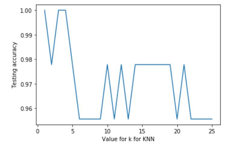
163 |
164 | #### STEP 4: MAKE PREDICTIONS
165 |
166 | Now we are going to choose an appropriate value of K as 5 for our model. So this is going to be our final model which is going to make predictions.
167 |
168 | ```
169 | >>> knn = KNeighborsClassifier(n_neighbors=5)
170 | >>> knn.fit(data,target)
171 | >>> target_Classes = {0:'iris_setosa', 1:'iris_versicolor', 2:'iris_verginica'}
172 | >>> x_new = [[4,3,1,2],
173 | ... [5,4,1,3]]
174 | >>> y_predict = knn.predict(x_new)
175 | >>> print('First Predictions -> ',target_Classes[y_predict[1]])
176 | >>> print('Second Predictions -> ',target_Classes[y_predict[0]])
177 |
178 |
179 | OUTPUT:
180 |
181 | First Predictions -> iris_setosa
182 | Second Predictions -> iris_setosa
183 | ```
184 |
185 | #### PROS
186 | - KNN classifier algorithm is used to solve both regression, classification, and multi-classification problem
187 | - KNN classifier algorithms can adapt easily to changes in real-time inputs.
188 | - We do not have to follow any special requirements before applying KNN.
189 |
190 | #### Cons
191 |
192 | - KNN performs well in a limited number of input variables. So, it’s really challenging to estimate the performance of new data as the number of variables increases. Thus, it is called the curse of dimensionality. In the modern scientific era, increasing quantities of data are being produced and collected. How, for target_class in machine learning, too much data can be a bad thing. At a certain level, additional features or dimensions will decrease the precision of a model, because more data has to be generalized. Thus, this is recognized as the “Curse of dimensionality”.
193 | - KNN requires data that is normalized and also the KNN algorithm cannot deal with the missing value problem.
194 | - The biggest problem with the KNN from scratch is finding the correct neighbor number.
195 |
196 | # 💥 ESSENCE OF THE KNN ALGORITHM IN ONE PICTURE!
197 |
198 | 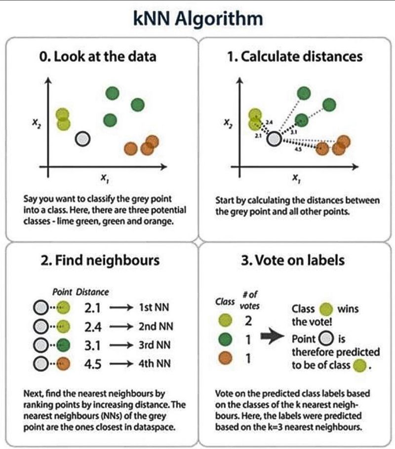
199 |
--------------------------------------------------------------------------------
/ML from Scratch/Naive Bayes/README.md:
--------------------------------------------------------------------------------
1 | # 1. NAIVE BAYES ALGORITHM FROM SCRATCH
2 |
3 | Naive Bayes is a classification algorithm based on the “Bayes Theorem”. So let’s get introduced to the Bayes Theorem first.
4 |
5 | 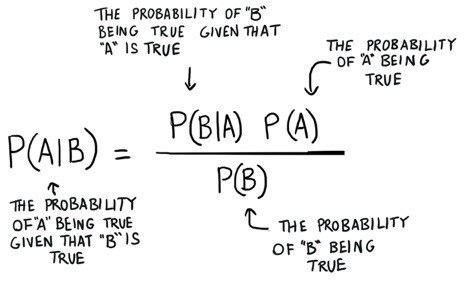
6 |
7 | Bayes Theorem is used to find the probability of an event occurring given the probability of another event that has already occurred. Here _**B**_ is the evidence and _**A**_ is the hypothesis. Here _**P(A)**_ is known as prior, _**P(A/B)**_ is posterior, and _**P(B/A)**_ is the likelihood.
8 |
9 | _**Posterior**_ = $\frac{prior \times likelihood} {evidence}$
10 |
11 | ## 1.1 NAIVE BAYES ALGORITHM
12 |
13 | The name Naive is used because the presence of one independent feature doesn’t affect (influence or change the value of) other features. The most important assumption that Naive Bayes makes is that all the features are independent of each other. Being less prone to overfitting, Naive Bayes algorithm works on Bayes theorem to predict unknown data sets.
14 |
15 | **EXAMPLE**:
16 |
17 | | AGE | INCOME | STUDENT | CREDIT | BUY COMPUTER |
18 | | :-: | :----: | :-----: | :----: | :----------: |
19 | | Youth | High | No | Fair | No |
20 | | Youth | High | No | Excellent | No |
21 | | Middle Age | High | No | Fair | Yes |
22 | | Senior | Medium | No | Fair | Yes |
23 | | Senior | Low | Yes | Fair | Yes |
24 | | Senior | Low | Yes | Excellent | No |
25 | | Middle Age | Low | Yes | Excellent | Yes |
26 | | Youth | Medium | No | Fair | No |
27 | | Youth | Low | Yes | Fair | Yes |
28 | | Senior | Medium | Yes | Fair | Yes |
29 | | Youth | Medium | Yes | Excellent | Yes |
30 | | Middle Age | Medium | No | Excellent | Yes |
31 | | Middle Age | High | Yes | Fair | Yes |
32 | | Senior | Medium | No | Excellent | No |
33 |
34 | We are given a table that contains a dataset about **age**, **income**, **student**, **credit-rating**, **buying a computer**, and their respective features. From the above dataset, we need to find whether a youth student with medium income having a fair credit rating buys a computer or not.
35 |
36 | i.e. B = (Youth, Medium, Yes, Flair)
37 |
38 | In the above dataset, we can apply the Bayesian theorem.
39 |
40 | P(A|B) = $\frac{P(B|A) \times P(A)}{P(B)}$
41 |
42 | Where,
43 | **A** = ( Yes / No ) under buying computer
44 | **B** = ( Youth, Medium, Student, Fair)
45 |
46 | So, **P(A/B)** means the probability of buying a computer given that conditions are “**Youth age**”, “**Medium Income**”, “**Student**”, and “**fair credit-rating**”.
47 |
48 | **ASSUMPTION**:
49 |
50 | Before starting, we assume that all the given features are independent of each other.
51 |
52 | ### STEP 1: CALCULATE PROBABILITIES OF BUYING A COMPUTER FROM ABOVE DATASET
53 |
54 | | Buy Computer | Count | Probability |
55 | | :----------: | :------: | :--------: |
56 | | Yes | 9 | 9/14 |
57 | | No | 5 | 5/14 |
58 | |Total | 14 | |
59 |
60 | ### STEP 2: CALCULATE PROBABILITIES UNDER CREDIT-RATING BUYING A COMPUTER FROM THE ABOVE DATASET
61 |
62 | 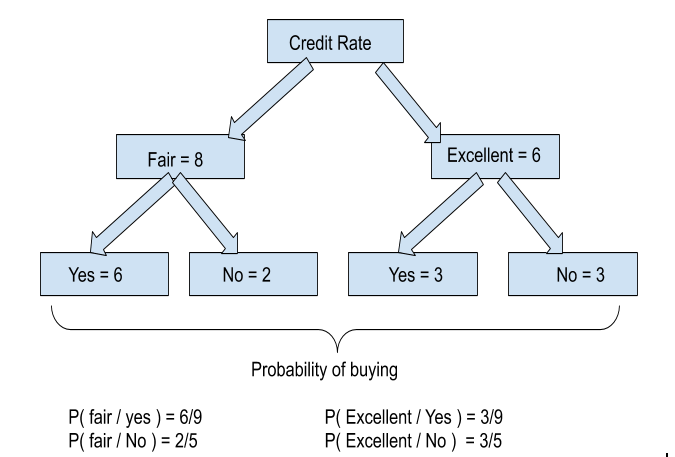
63 |
64 | Let’s understand how we calculated the above probabilities. From the table we can see that there are 8 fair credit ratings among which 6 buy computers and 2 don’t buy. Similarly, 6 have excellent credit ratings among which 3 buy computers and 3 don’t. As a whole 9 (6+3) buy computers and 5 (2+5) don’t.
65 |
66 | P(fair / Yes) means the probability of credit rating being fair when someone buys a computer. Hence, P(fair / Yes) = P( fair buying computer) / P ( total number of buying computer) i.e. 6/9.
67 |
68 | ### STEP 3: CALCULATE PROBABILITIES UNDER STUDENT BUYING A COMPUTER FROM THE ABOVE DATASET
69 |
70 | 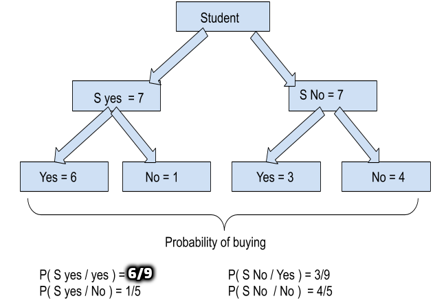
71 |
72 | #### STEP 4: CALCULATE PROBABILITIES UNDER INCOME LEVEL BUYING A COMPUTER FROM THE ABOVE DATASET
73 |
74 | P( High / Yes ) = 2/9
75 | P( Mid / Yes ) = 4/9
76 | P( Low / Yes ) = 3/9
77 | P( High / No ) = 2/5
78 | P( Mid / No ) = 2/5
79 | P( Low / No ) = 1/5
80 |
81 | ### STEP 5: CALCULATE PROBABILITIES UNDER AGE LEVEL BUYING A COMPUTER FROM THE ABOVE DATASET
82 |
83 | P( Youth / Yes ) = 2/9
84 | P( Mid / Yes ) = 4/9
85 | P( Senior / Yes ) = 3/9
86 | P( Youth / No ) = 3/5
87 | P( Mid / No ) = 0
88 | P( Senior / No ) = 2/5
89 |
90 | **CALCULATION**
91 |
92 | We have,
93 | B = ( Youth, Medium, Student, Fair)
94 |
95 | ```
96 | P(Yes) * P(B / Yes ) = P(Yes) * P( Youth / Yes ) * P( Mid / Yes) * P( S Yes / Yes) * P( Fair / Yes)
97 | = 9/14 * 2/9 * 4/9 * 6/9 * 6/9
98 | = 0.02821
99 | P(No) * P(B / No ) = P(No) * P( Youth / No ) * P( Mid / No) * P( S Yes / No) * P( Fair / No)
100 | = 5/14 * 3/5 * 2/5 * 1/5 * 2/5
101 | = 0.04373
102 | ```
103 | Hence,
104 |
105 | ```
106 | P(Yes / B) = P(Yes) * P(B / Yes ) / P(B)
107 | = 0.02821 / 0.04373
108 | = 0.645
109 |
110 | P(No / B) = P(No) * P(B / No ) / P(B)
111 | = 0.0068 / 0.04373
112 | = 0.155
113 | ```
114 |
115 | Here, P(Yes / B) is greater than P(No / B) i.e posterior Yes is greater than posterior No. So the class B ( Youth, Mid, yes, fair) buys a computer.
116 |
117 | ## 1.2. NAIVE BAYES FROM SCRATCH
118 |
119 | ** Classify whether a given person is a male or a female based on the measured features. The features include height, weight, and foot size.
120 | **
121 |
122 | 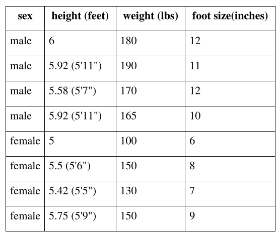
123 |
124 | Now, defining a dataframe which consists if above provided data.
125 | ```
126 | import pandas as pd
127 | import numpy as np
128 |
129 | # Create an empty dataframe
130 | data = pd.DataFrame()
131 |
132 | # Create our target variable
133 | data['Gender'] = ['male','male','male','male','female','female','female','female']
134 |
135 | # Create our feature variables
136 | data['Height'] = [6,5.92,5.58,5.92,5,5.5,5.42,5.75]
137 | data['Weight'] = [180,190,170,165,100,150,130,150]
138 | data['Foot_Size'] = [12,11,12,10,6,8,7,9]
139 | ```
140 |
141 | Creating another data frame containing the feature value of height as 6 feet, weight as 130 lbs and foot size as 8 inches. using Naive Bayes from scratch we are trying to find whether the gender is male or female.
142 |
143 | ```
144 | # Create an empty dataframe
145 | person = pd.DataFrame()
146 |
147 | # Create some feature values for this single row
148 | person['Height'] = [6]
149 | person['Weight'] = [130]
150 | person['Foot_Size'] = [8]
151 | ```
152 |
153 | Calculating the total number of males and females and their probabilities i.e priors:
154 |
155 | ```
156 | # Number of males
157 | n_male = data['Gender'][data['Gender'] == 'male'].count()
158 |
159 | # Number of males
160 | n_female = data['Gender'][data['Gender'] == 'female'].count()
161 |
162 | # Total rows
163 | total_ppl = data['Gender'].count()
164 |
165 | # Number of males divided by the total rows
166 | P_male = n_male/total_ppl
167 |
168 | # Number of females divided by the total rows
169 | P_female = n_female/total_ppl
170 | ```
171 | Calculating mean and variance of male and female of the feature height, weight and foot size.
172 |
173 | ```
174 | # Group the data by gender and calculate the means of each feature
175 | data_means = data.groupby('Gender').mean()
176 |
177 | # Group the data by gender and calculate the variance of each feature
178 | data_variance = data.groupby('Gender').var()
179 | ```
180 | 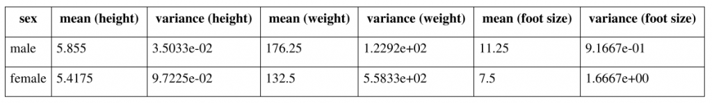
181 |
182 | **Formula**:
183 |
184 | * posterior (male) = P(male)*P(height|male)*P(weight|male)*P(foot size|male) / evidence
185 | * posterior (female) = P(female)*P(height|female)*P(weight|female)*P(foot size|female) / evidence
186 | * Evidence = P(male)*P(height|male)*P(weight|male)*P(foot size|male) + P(female) * P(height|female) * P(weight|female)*P(foot size|female)
187 |
188 | The evidence may be ignored since it is a positive constant. (Normal distributions are always positive.)
189 |
190 | **CALCULATION**:
191 |
192 | 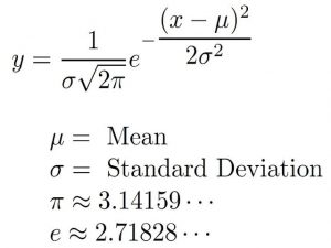
193 |
194 | **Calculation of P(height | Male )**
195 |
196 | mean of the height of male = 5.855
197 | variance ( Square of S.D.) of the height of a male is square of 3.5033e-02 and x i.e. given height is 6 feet
198 | Substituting the values in the above equation we get P(height | Male ) = 1.5789
199 |
200 | ```
201 | # Create a function that calculates p(x | y):
202 | def p_x_given_y(x, mean_y, variance_y):
203 |
204 | # Input the arguments into a probability density function
205 | p = 1/(np.sqrt(2*np.pi*variance_y)) * np.exp((-(x-mean_y)**2)/(2*variance_y))
206 |
207 | # return p
208 | return p
209 | ```
210 |
211 | Similarly,
212 |
213 | P(weight|male) = 5.9881e-06
214 | P(foot size|male) = 1.3112e-3
215 | P(height|female) = 2.2346e-1
216 | P(weight|female) = 1.6789e-2
217 | P(foot size|female) = 2.8669e-1
218 |
219 | Posterior (male)*evidence = P(male)*P(height|male)*P(weight|male)*P(foot size|male) = 6.1984e-09
220 | Posterior (female)*evidence = P(female)*P(height|female)*P(weight|female)*P(foot size|female)= 5.3778e-04
221 |
222 | **CONCLUSION**
223 | Since Posterior (female)*evidence > Posterior (male)*evidence, the sample is female.
224 |
225 | ## 1.3. NAIVE BAYES USING SCIKIT-LEARN
226 |
227 | ```
228 | import pandas as pd
229 | import numpy as np
230 |
231 | # Create an empty dataframe
232 | data = pd.DataFrame()
233 |
234 | # Create our target variable
235 | data['Gender'] = [1,1,1,1,0,0,0,0] #1 is male
236 | # Create our feature variables
237 | data['Height'] = [6,5.92,5.58,5.92,5,5.5,5.42,5.75]
238 | data['Weight'] = [180,190,170,165,100,150,130,150]
239 | data['Foot_Size'] = [12,11,12,10,6,8,7,9]
240 | ```
241 |
242 | Though we have very small dataset, we are dividing the dataset into train and test do that it can be used in other model prediction. We are importing gnb() from sklearn and we are training the model with out dataset.
243 |
244 | ```
245 | X = data.drop(['Gender'],axis=1)
246 | y=data.Gender
247 |
248 |
249 | # splitting X and y into training and testing sets
250 | from sklearn.model_selection import train_test_split
251 | X_train, X_test, y_train, y_test = train_test_split(X, y, test_size=0.4, random_state=1)
252 |
253 | # training the model on training set
254 | from sklearn.naive_bayes import GaussianNB
255 | gnb = GaussianNB()
256 | gnb.fit(X_train, y_train)
257 |
258 | # making predictions on the testing set
259 | y_pred = gnb.predict(X_test)
260 | ```
261 |
262 | Now, our model is ready. Let’s use this model to predict on new data.
263 |
264 | ```
265 | # Create our target variable
266 | data1 = pd.DataFrame()
267 |
268 | # Create our feature variables
269 | data1['Height'] = [6]
270 | data1['Weight'] = [130]
271 | data1['Foot_Size'] = [8]
272 |
273 | y_pred = gnb.predict(data1)
274 | if y_pred==0:
275 | print ("female")
276 | else:
277 | print ("male")
278 |
279 | Output: Female
280 | ```
281 |
282 | **CONCLUSION**
283 |
284 | We have come to an end of Naive Bayes from Scratch. If you have any queries, feedback, or suggestions then you can leave a comment or mail on **info@sunilghimire.com.np**. See you in the next tutorial.
285 |
286 | ### Stay safe !! Happy Coding !!!
287 |
--------------------------------------------------------------------------------
/README.md:
--------------------------------------------------------------------------------
1 | # Implementation of Machine Learning Algorithm from Scratch
2 | Learn Machine Learning from basic to advance and develop Machine Learning Models from Scratch in Python
3 |
4 | ## 1. WHAT YOU WILL LEARN?
5 | * Obtain a solid understand of machine learning in general from basic to advance
6 | * Complete tutorial about basic packages like NumPy and Pandas
7 | * Data Preprocessing and Data Visualization
8 | * Have an understand of Machine Learning and how to apply it in your own programs
9 | * Understanding the concept behind the algorithms
10 | * Knowing how to optimize hyperparameters of your models
11 | * Learn how to develop models based on the requirement of your future business
12 | * Potential for a new job in the future
13 |
14 | ## 2. DESCRIPTION
15 | Are you interested in Data Science and Machine Learning, but you don’t have any background, and you find the concepts confusing?
16 | Are you interested in programming in Python, but you always afraid of coding?
17 |
18 | 😊I think this repo is for you!😊
19 |
20 | Even you are familiar with machine learning, this repo can help you to review all the techniques and understand the concept behind each term.
21 | This repo is completely categorized, and I don’t start from the middle! I actually start the concept of every term, and then I try to implement it in Python step by step. The structure of the course is as follows:
22 |
23 | ## 3. WHO THIS REPO IS FOR:
24 | * Anyone with any background that interested in Data Science and Machine Learning with at least high school (+2) knowledge in mathematics
25 | * Beginners, intermediate, and even advanced students in the field of Artificial Intelligence (AI), Data Science (DS), and Machine Learning (ML)
26 | * Students in college that looking for securing their future jobs
27 | * Students that look forward to excel their Final Year Project by learning Machine Learning
28 | * Anyone who afraid of coding in Python but interested in Machine Learning concepts
29 | * Anyone who wants to create new knowledge on the different dataset using machine learning
30 | * Students who want to apply machine learning models in their projects
31 |
32 | ## 4. Contents
33 | * [Useful Commands](#useful-commands)
34 | * [Installation](#installation)
35 | * [Reality vs Expectation](#reality-vs-expectation)
36 | * [Machine Learning from Beginner to Advanced](#machine-learning-from-beginner-to-advanced)
37 | * [Scratch Implementation](#scratch-implementation)
38 | * [Mathematical Implementation](#mathematical-implementation)
39 | * [Machine Learning Interview Questions with Answers](#machine-learning-interview-questions-with-answers)
40 | * [Essential Machine Learning Formulas](#essential-machine-learning-formulas)
41 | * [Pratice Guide for Data Science Learning](#pratice-guide-for-data-science-learning)
42 |
43 | # Useful Resources
44 | | Title | Repository |
45 | |------ | :----------: |
46 | | USEFUL GIT COMMANDS FOR EVERYDAY USE | [🔗](https://github.com/ghimiresunil/Git-Cheat-Sheet)|
47 | | MOST USEFUL LINUX COMMANDS EVERYONE SHOULD KNOW | [🔗](https://github.com/ghimiresunil/Linux-Guide-For-All)|
48 | | AWESOME ML TOOLBOX| [🔗](https://github.com/ghimiresunil/Awesome-ML-Toolbox)|
49 |
50 | # Installation
51 | | Title | Repository |
52 | |------ | :----------: |
53 | |INSTALL THE ANACONDA PYTHON ON WINDOWS AND LINUX | [🔗](https://github.com/ghimiresunil/Implementation-of-Machine-Learning-Algorithm-from-Scratch/blob/main/Installation/install_anaconda_python.md)|
54 |
55 | # Reality vs Expectation
56 | | Title | Repository |
57 | |------ | :----------: |
58 | | IS AI OVERHYPED? REALITY VS EXPECTATION |[🔗](https://github.com/ghimiresunil/Implementation-of-Machine-Learning-Algorithm-from-Scratch/blob/main/Reality%20vs%20Expectation/Is%20AI%20Overhyped%3F%20Reality%20vs%20Expectation.md)|
59 |
60 | # Machine Learning from Beginner to Advanced
61 | | Title | Repository |
62 | |------ | :----------: |
63 | |HISTORY OF MATHEMATICS, AI & ML - HISTORY & MOTIVATION| [🔗](https://github.com/ghimiresunil/Implementation-of-Machine-Learning-Algorithm-from-Scratch/blob/main/Machine%20Learning%20from%20Beginner%20to%20Advanced/mathematics_ai_ml_history_motivation.md)|
64 | | INTRODUCTION TO ARTIFICIAL INTELLIGENCE & MACHINE LEARNING |[🔗](https://github.com/ghimiresunil/Implementation-of-Machine-Learning-Algorithm-from-Scratch/blob/main/Machine%20Learning%20from%20Beginner%20to%20Advanced/Introduction%20to%20ML%20and%20AI.md)|
65 | | KEY TERMS USED IN MACHINE LEARNING | [🔗](https://github.com/ghimiresunil/Implementation-of-Machine-Learning-Algorithm-from-Scratch/blob/main/Machine%20Learning%20from%20Beginner%20to%20Advanced/Key%20terms%20used%20in%20ML.md) |
66 | |PERFORMANCE METRICS IN MACHINE LEARNING CLASSIFICATION MODEL| [🔗](https://github.com/ghimiresunil/Implementation-of-Machine-Learning-Algorithm-from-Scratch/blob/main/Machine%20Learning%20from%20Beginner%20to%20Advanced/Classification%20Performance%20Metrics.md) |
67 | |PERFORMANCE METRICS IN MACHINE LEARNING REGRESSION MODEL| [🔗](https://github.com/ghimiresunil/Implementation-of-Machine-Learning-Algorithm-from-Scratch/blob/main/Machine%20Learning%20from%20Beginner%20to%20Advanced/Regression%20Performance%20Metrics.md) |
68 |
69 | # Scratch Implementation
70 | | Title | Repository |
71 | |------ | :----------: |
72 | |LINEAR REGRESSION FROM SCRATCH| [🔗](https://github.com/ghimiresunil/Implementation-of-Machine-Learning-Algorithm-from-Scratch/tree/main/ML%20from%20Scratch/Linear%20Regression)|
73 | |LOGISTIC REGRESSION FROM SCRATCH| [🔗](https://github.com/ghimiresunil/Implementation-of-Machine-Learning-Algorithm-from-Scratch/tree/main/ML%20from%20Scratch/Logistic%20Regression)|
74 | |NAIVE BAYES FROM SCRATCH| [🔗](https://github.com/ghimiresunil/Implementation-of-Machine-Learning-Algorithm-from-Scratch/tree/main/ML%20from%20Scratch/Naive%20Bayes)|
75 | |DECISION TREE FROM SCRATCH|[🔗](https://github.com/ghimiresunil/Implementation-of-Machine-Learning-Algorithm-from-Scratch/blob/main/ML%20from%20Scratch/Decision%20Tree/README.md)|
76 | |RANDOM FOREST FROM SCRATCH|[🔗](https://github.com/ghimiresunil/Implementation-of-Machine-Learning-Algorithm-from-Scratch/tree/main/ML%20from%20Scratch/Random%20Forest)|
77 | | K NEAREST NEIGHBOUR | [🔗](https://github.com/ghimiresunil/Implementation-of-Machine-Learning-Algorithm-from-Scratch/tree/main/ML%20from%20Scratch/KNN)|
78 | | NAIVE BAYES | [🔗](https://github.com/ghimiresunil/Implementation-of-Machine-Learning-Algorithm-from-Scratch/tree/main/ML%20from%20Scratch/Naive%20Bayes)|
79 | | K MEANS CLUSTERING | [🔗](https://github.com/ghimiresunil/Implementation-of-Machine-Learning-Algorithm-from-Scratch/tree/main/ML%20from%20Scratch/K%20Means%20Clustering)|
80 |
81 | # Mathematical Implementation
82 | | Title | Repository |
83 | |------ | :----------: |
84 | |CONFUSION MATRIX FOR YOUR MULTI-CLASS ML MODEL| [🔗](https://github.com/ghimiresunil/Implementation-of-Machine-Learning-Algorithm-from-Scratch/blob/main/Mathematical%20Implementation/confusion_matrix.md)|
85 |
86 | # Machine Learning Interview Questions with Answers
87 | | Title | Repository |
88 | |------ | :----------: |
89 | |50 QUESTIONS ON STATISTICS & MACHINE LEARNING – CAN YOU ANSWER? | [🔗](https://graspcoding.com/50-questions-on-statistics-machine-learning-can-you-answer/)|
90 |
91 | # Essential Machine Learning Formulas
92 | | Title | Repository |
93 | |------ | :----------: |
94 | |MOSTLY USED MACHINE LEARNING FORMULAS |[🔗](https://github.com/ghimiresunil/Machine-Learning-Formulas)|
95 |
96 | # Pratice Guide for Data Science Learning
97 | | Title | Repository |
98 | |------ | :----------: |
99 | | Research Guide for FYP | [🔗](https://github.com/ghimiresunil/Implementation-of-Machine-Learning-Algorithm-from-Scratch/blob/main/Pratice%20Guide/research_guide_for_fyp.md)|
100 | |The Intermediate Guide to 180 Days Data Science Learning Plan|[🔗](https://graspcoding.com/the-intermediate-guide-to-180-days-data-science-learning-plan/)|
101 |
102 | ***
103 |
104 | ### Algorithm Pros and Cons
105 |
106 | - KN Neighbors \
107 | ✔ Simple, No training, No assumption about data, Easy to implement, New data can be added seamlessly, Only one hyperparameter \
108 | ✖ Doesn't work well in high dimensions, Sensitive to noisy data, missing values and outliers, Doesn't work well with large data sets — cost of calculating distance is high, Needs feature scaling, Doesn't work well on imbalanced data, Doesn't deal well with missing values
109 |
110 | - Decision Tree \
111 | ✔ Doesn't require standardization or normalization, Easy to implement, Can handle missing values, Automatic feature selection \
112 | ✖ High variance, Higher training time, Can become complex, Can easily overfit
113 |
114 | - Random Forest \
115 | ✔ Left-out data can be used for testing, High accuracy, Provides feature importance estimates, Can handle missing values, Doesn't require feature scaling, Good performance on imbalanced datasets, Can handle large dataset, Outliers have little impact, Less overfitting \
116 | ✖ Less interpretable, More computational resources, Prediction time high
117 |
118 | - Linear Regression \
119 | ✔ Simple, Interpretable, Easy to Implement \
120 | ✖ Assumes linear relationship between features, Sensitive to outliers
121 |
122 | - Logistic Regression \
123 | ✔ Doesn’t assume linear relationship between independent and dependent variables, Output can be interpreted as probability, Robust to noise \
124 | ✖ Requires more data, Effective when linearly separable
125 |
126 | - Lasso Regression (L1) \
127 | ✔ Prevents overfitting, Selects features by shrinking coefficients to zero \
128 | ✖ Selected features will be biased, Prediction can be worse than Ridge
129 |
130 | - Ridge Regression (L2) \
131 | ✔ Prevents overfitting \
132 | ✖ Increases bias, Less interpretability
133 |
134 | - AdaBoost \
135 | ✔ Fast, Reduced bias, Little need to tune \
136 | ✖ Vulnerable to noise, Can overfit
137 |
138 | - Gradient Boosting \
139 | ✔ Good performance \
140 | ✖ Harder to tune hyperparameters
141 |
142 | - XGBoost \
143 | ✔ Less feature engineering required, Outliers have little impact, Can output feature importance, Handles large datasets, Good model performance, Less prone to overfitting \
144 | ✖ Difficult to interpret, Harder to tune as there are numerous hyperparameters
145 |
146 | - SVM \
147 | ✔ Performs well in higher dimensions, Excellent when classes are separable, Outliers have less impact \
148 | ✖ Slow, Poor performance with overlapping classes, Selecting appropriate kernel functions can be tricky
149 |
150 | - Naïve Bayes \
151 | ✔ Fast, Simple, Requires less training data, Scalable, Insensitive to irrelevant features, Good performance with high-dimensional data \
152 | ✖ Assumes independence of features
153 |
154 | - Deep Learning \
155 | ✔ Superb performance with unstructured data (images, video, audio, text) \
156 | ✖ (Very) long training time, Many hyperparameters, Prone to overfitting
157 |
158 |
159 | ***
160 |
161 | ***
162 | ### AI/ML dataset
163 |
164 | | Source | Link |
165 | |------ | :----------: |
166 | | Google Dataset Search – A search engine for datasets: | [🔗](https://datasetsearch.research.google.com/) |
167 | | IBM’s collection of datasets for enterprise applications | [🔗](https://developer.ibm.com/exchanges/data/ ) |
168 | | Kaggle Datasets | [🔗](https://www.kaggle.com/datasets) |
169 | | Huggingface Datasets – A Python library for loading NLP datasets | [🔗](https://github.com/huggingface/datasets) |
170 | | A large list organized by application domain | [🔗](https://github.com/awesomedata/awesome-public-datasets) |
171 | | Computer Vision Datasets (a really large list) | [🔗](https://homepages.inf.ed.ac.uk/rbf/CVonline/Imagedbase.htm) |
172 | | Datasetlist – Datasets by domain | [🔗](https://www.datasetlist.com/) |
173 | | OpenML – A search engine for curated datasets and workflows| [🔗](https://www.openml.org/search?type=data ) |
174 | | Papers with Code – Datasets with benchmarks | [🔗](https://www.paperswithcode.com/datasets) |
175 | | Penn Machine Learning Benchmarks | [🔗](https://github.com/EpistasisLab/pmlb/tree/master/datasets) |
176 | | VisualDataDiscovery (for Computer Vision) | [🔗](https://www.visualdata.io/discovery) |
177 | | UCI Machine Learning Repository | [🔗](https://archive.ics.uci.edu/ml/index.php) |
178 | | Roboflow Public Datasets for computer vision | [🔗](https://public.roboflow.com/) |
179 | ***
180 |
--------------------------------------------------------------------------------
/ML from Scratch/K Means Clustering/README.md:
--------------------------------------------------------------------------------
1 | # 1. K-Means Clustering From Scratch Python
2 |
3 | 
4 |
5 |
6 | In this article, I will cover k-means clustering from scratch. In general, Clustering is defined as the grouping of data points such that the data points in a group will be similar or related to one another and different from the data points in another group. The goal of clustering is to determine the intrinsic grouping in a set of unlabelled data.
7 |
8 | K- means is an unsupervised partitional clustering algorithm that is based on grouping data into k – numbers of clusters by determining centroid using the Euclidean or Manhattan method for distance calculation. It groups the object based on minimum distance.
9 |
10 | 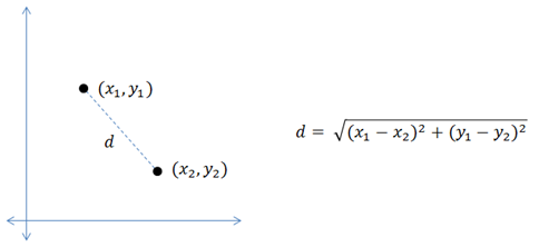
11 |
12 |
13 | ## 1.1. ALGORITHM
14 |
15 | - First, initialize the number of clusters, K (Elbow method is generally used in selecting the number of clusters )
16 | - Randomly select the k data points for centroid. A centroid is the imaginary or real location representing the center of the cluster.
17 | - Categorize each data items to its closest centroid and update the centroid coordinates calculating the average of items coordinates categorized in that group so far
18 | - Repeat the process for a number of iterations till successive iterations clusters data items into the same group
19 |
20 | ## 1.2. HOW IT WORKS ?
21 |
22 | In the beginning, the algorithm chooses k centroids in the dataset randomly after shuffling the data. Then it calculates the distance of each point to each centroid using the euclidean distance calculation method. Each centroid assigned represents a cluster and the points are assigned to the closest cluster. At the end of the first iteration, the centroid values are recalculated, usually taking the arithmetic mean of all points in the cluster. In every iteration, new centroid values are calculated until successive iterations provide the same centroid value.
23 |
24 | Let’s kick off K-Means Clustering Scratch with a simple example: Suppose we have data points (1,1), (1.5,2), (3,4), (5,7), (3.5,5), (4.5,5), (3.5,4.5). Let us suppose k = 2 i.e. dataset should be grouped in two clusters. Here we are using the Euclidean distance method.
25 |
26 | 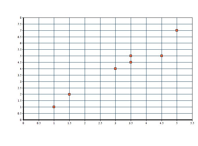
27 |
28 | **Step 01**: It is already defined that k = 2 for this problem
29 | **Step 02**: Since k = 2, we are randomly selecting two centroid as c1(1,1) and c2(5,7)
30 | **Step 03**: Now, we calculate the distance of each point to each centroid using the euclidean distance calculation method:
31 |
32 | 
33 |
34 | **1.2.1. ITERATION 01**
35 |
36 | |X1 |Y1 |**X2**| **Y2** |**D1** |X1| Y1| **X2**| **Y2**| **D2**| Remarks|
37 | |:------:| :------:| :----------:|:----------:|:----------:|:----------:|:----------:|:----------:|:----------:|:----------:|:----------:|
38 | |1 |1 |1 |1 |0 |1 |1 |5 |7 |7.21 |D1D2 : (5,7) belongs to c2|
42 | |3.5 |5 |1 |1 |4.72 |3.5 |5 |5 |7 |2.5 |D1>D2 : (3.5,5) belongs to c2|
43 | |4.5 |5 |1 |1 |5.32 |4.5 |5 |5 |7 |2.06 |D1>D2 : (5.5,5) belongs to c2|
44 | |3.5 |4.5 |1 |1 |4.3 |3.5 |4.5 |5 |7 |2.91 |D1>D2 : (3.5,4.5) belongs to c2|
45 |
46 | _**Note**_: D1 & D2 are euclidean distance between centroid **(x2,y2)** and data points **(x1,y1)**
47 |
48 | In cluster c1 we have (1,1), (1.5,2) and (3,4) whereas centroid c2 contains (5,7), (3.5,5), (4.5,5) & (3.5,4.5). Here, a new centroid is the algebraic mean of all the data items in a cluster.
49 |
50 | **C1(new)** = ( (1+1.5+3)/3 , (1+2+4)/3) = **(1.83, 2.33)**
51 | **C2(new)** = ((5+3.5+4.5+3.5)/4, (7+5+5+4.5)/4) = **(4.125, 5.375)**
52 |
53 |
54 | 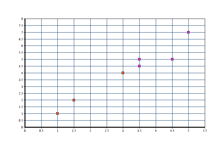
55 |
56 |
57 | **1.2.2. ITERATION 02**
58 |
59 | |X1 |Y1 |**X2**| **Y2** |**D1** |X1| Y1| **X2**| **Y2**| **D2**| Remarks|
60 | |:------:| :------:| :----------:|:----------:|:----------:|:----------:|:----------:|:----------:|:----------:|:----------:|:----------:|
61 | |1 |1 |1.83 |2.33 |1.56 |1 |1 |4.12 |5.37 |5.37 |(1,1) belongs to c1|
62 | |1.5 |2 |1.83 |2.33 |0.46 |1.5 |2 |4.12 |5.37 |4.27 |(1.5,2) belongs to c1|
63 | |3 |4 |1.83 |2.33 |2.03 |3 |4 |4.12 |5.37 |1.77 |(3,4) belongs to c2|
64 | |5 |7 |1.83 |2.33 |5.64 |5 |7 |4.12 |5.37 |1.84 |(5,7) belongs to c2|
65 | |3.5 |5 |1.83 |2.33 |3.14 |3.5 |5 |4.12 |5.37 |0.72 |(3.5,5) belongs to c2|
66 | |4.5 |5 |1.83 |2.33 |3.77 |4.5 |5 |4.12 |5.37 |0.53 |(5.5,5) belongs to c2|
67 | |3.5 |4.5 |1.83 |2.33 |2.73 |3.5 |4.5 |4.12 |5.37 |1.07 |(3.5,4.5) belongs to c2|
68 |
69 | In cluster c1 we have (1,1), (1.5,2) ) whereas centroid c2 contains (3,4),(5,7), (3.5,5), (4.5,5) & (3.5,4.5). Here, new centroid is the algebraic mean of all the data items in a cluster.
70 |
71 | **C1(new)** = ( (1+1.5)/2 , (1+2)/2) = **(1.25,1.5)**
72 | **C2(new)** = ((3+5+3.5+4.5+3.5)/5, (4+7+5+5+4.5)/5) = **(3.9, 5.1)**
73 |
74 | 
75 |
76 |
77 | **1.2.3. ITERATION 03**
78 |
79 | |X1 |Y1 |**X2**| **Y2** |**D1** |X1| Y1| **X2**| **Y2**| **D2**| Remarks|
80 | |:------:| :------:| :----------:|:----------:|:----------:|:----------:|:----------:|:----------:|:----------:|:----------:|:----------:|
81 | |1 |1 |1.25 |1.5 |0.56 |1 |1 |3.9 |5.1 |5.02 |(1,1) belongs to c1|
82 | |1.5 |2 |1.25 |1.5 |0.56 |1.5 |2 |3.9 |5.1 |3.92 |(1.5,2) belongs to c1|
83 | |3 |4 |1.25 |1.5 |3.05 |3 |4 |3.9 |5.1 |1.42 |(3,4) belongs to c2|
84 | |5 |7 |1.25 |1.5 |6.66 |5 |7 |3.9 |5.1 |2.19 |(5,7) belongs to c2|
85 | |3.5 |5 |1.25 |1.5 |4.16 |3.5 |5 |3.9 |5.1 |0.41 |(3.5,5) belongs to c2|
86 | |4.5 |5 |1.25 |1.5 |4.77 |4.5 |5 |3.9 |5.1 |0.60 |(5.5,5) belongs to c2|
87 | |3.5 |4.5 |1.25 |1.5 |3.75 |3.5 |4.5 |3.9 |5.1 |0.72 |(3.5,4.5) belongs to c2|
88 |
89 | In cluster c1 we have (1,1), (1.5,2) ) whereas centroid c2 contains (3,4),(5,7), (3.5,5), (4.5,5) & (3.5,4.5). Here, new centroid is the algebraic mean of all the data items in a cluster.
90 |
91 | **C1(new)** = ( (1+1.5)/2 , (1+2)/2) = **(1.25,1.5)**
92 | **C2(new)** = ((3+5+3.5+4.5+3.5)/5, (4+7+5+5+4.5)/5) = **(3.9, 5.1)**
93 |
94 | **Step 04**: In the 2nd and 3rd iteration, we obtained the same centroid points. Hence clusters of above data point is :
95 |
96 |
97 | # 2. K-Means Clustering Scratch Code
98 |
99 | So far, we have learnt about the introduction to the K-Means algorithm. We have learnt in detail about the mathematics behind the K-means clustering algorithm and have learnt how Euclidean distance method is used in grouping the data items in K number of clusters. Here were are implementing K-means clustering from scratch using python. But the problem is how to choose the number of clusters? In this example, we are assigning the number of clusters ourselves and later we will be discussing various ways of finding the best number of clusters.
100 |
101 | ```
102 | import pandas as pd
103 | import numpy as np
104 | import random as rd
105 | import matplotlib.pyplot as plt
106 | import math
107 |
108 | class K_Means:
109 |
110 | def __init__(self, k=2, tolerance = 0.001, max_iter = 500):
111 | self.k = k
112 | self.max_iterations = max_iter
113 | self.tolerance = tolerance
114 | ```
115 |
116 | We have defined a K-means class with init consisting default value of k as 2, error tolerance as 0.001, and maximum iteration as 500.
117 | Before diving into the code, let’s remember some mathematical terms involved in K-means clustering:- centroids & euclidean distance. On a quick note centroid of a data is the average or mean of the data and Euclidean distance is the distance between two points in the coordinate plane calculated using Pythagoras theorem.
118 |
119 | ```
120 | def euclidean_distance(self, point1, point2):
121 | #return math.sqrt((point1[0]-point2[0])**2 + (point1[1]-point2[1])**2 + (point1[2]-point2[2])**2) #sqrt((x1-x2)^2 + (y1-y2)^2)
122 | return np.linalg.norm(point1-point2, axis=0)
123 | ```
124 |
125 | We find the euclidean distance from each point to all the centroids. If you look for efficiency it is better to use the NumPy function (np.linalg.norm(point1-point2, axis=0))
126 |
127 | ```
128 | def fit(self, data):
129 | self.centroids = {}
130 | for i in range(self.k):
131 | self.centroids[i] = data[i]
132 | ```
133 |
134 | ### ASSIGNING CENTROIDS
135 |
136 | There are various methods of assigning k centroid initially. Mostly used is a random selection but let’s go in the most basic way. We assign the first k points from the dataset as the initial centroids.
137 |
138 | ```
139 | for i in range(self.max_iterations):
140 |
141 | self.classes = {}
142 | for j in range(self.k):
143 | self.classes[j] = []
144 |
145 |
146 | for point in data:
147 | distances = []
148 | for index in self.centroids:
149 | distances.append(self.euclidean_distance(point,self.centroids[index]))
150 | cluster_index = distances.index(min(distances))
151 | self.classes[cluster_index].append(point)
152 | ```
153 |
154 | Till now, we have defined the K-means class and initialized some default parameters. We have defined the euclidean distance calculation function and we have also assigned initial k clusters. Now, In order to know which cluster and data item belong to, we are calculating Euclidean distance from the data items to each centroid. Data item closest to the cluster belongs to that respective cluster.
155 |
156 | ```
157 | previous = dict(self.centroids)
158 | for cluster_index in self.classes:
159 | self.centroids[cluster_index] = np.average(self.classes[cluster_index], axis = 0)
160 |
161 | isOptimal = True
162 |
163 | for centroid in self.centroids:
164 | original_centroid = previous[centroid]
165 | curr = self.centroids[centroid]
166 | if np.sum((curr - original_centroid)/original_centroid * 100.0) > self.tolerance:
167 | isOptimal = False
168 | if isOptimal:
169 | break
170 | ```
171 |
172 | At the end of the first iteration, the centroid values are recalculated, usually taking the arithmetic mean of all points in the cluster. In every iteration, new centroid values are calculated until successive iterations provide the same centroid value.
173 |
174 | **CLUSTERING WITH DEMO DATA**
175 |
176 | We’ve now completed the K Means scratch code of this Machine Learning tutorial series. Now, let’s test our code by clustering with randomly generated data:
177 |
178 | ```
179 | #generate dummy cluster datasets
180 | # Set three centers, the model should predict similar results
181 | center_1 = np.array([1,1])
182 | center_2 = np.array([5,5])
183 | center_3 = np.array([8,1])
184 |
185 | # Generate random data and center it to the three centers
186 | cluster_1 = np.random.randn(100, 2) + center_1
187 | cluster_2 = np.random.randn(100,2) + center_2
188 | cluster_3 = np.random.randn(100,2) + center_3
189 |
190 | data = np.concatenate((cluster_1, cluster_2, cluster_3), axis = 0)
191 | ```
192 |
193 | Here we have created 3 groups of data of two-dimension with a different centre. We have defined the value of k as 3. Now, let’s fit the model created from scratch.
194 |
195 | ```
196 | k_means = K_Means(K)
197 | k_means.fit(data)
198 |
199 |
200 | # Plotting starts here
201 | colors = 10*["r", "g", "c", "b", "k"]
202 |
203 | for centroid in k_means.centroids:
204 | plt.scatter(k_means.centroids[centroid][0], k_means.centroids[centroid][1], s = 130, marker = "x")
205 |
206 | for cluster_index in k_means.classes:
207 | color = colors[cluster_index]
208 | for features in k_means.classes[cluster_index]:
209 | plt.scatter(features[0], features[1], color = color,s = 30
210 | ```
211 | 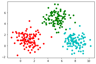
212 |
213 | ## 3. K-MEANS USING SCIKIT-LEARN
214 |
215 | ```
216 | from sklearn.cluster import KMeans
217 | center_1 = np.array([1,1])
218 | center_2 = np.array([5,5])
219 | center_3 = np.array([8,1])
220 |
221 | # Generate random data and center it to the three centers
222 | cluster_1 = np.random.randn(100,2) + center_1
223 | cluster_2 = np.random.randn(100,2) + center_2
224 | cluster_3 = np.random.randn(100,2) + center_3
225 |
226 | data = np.concatenate((cluster_1, cluster_2, cluster_3), axis = 0)
227 | kmeans = KMeans(n_clusters=3)
228 | kmeans.fit(data)
229 | plt.scatter(data[:,0],data[:,1], c=kmeans.labels_, cmap='rainbow')
230 | ```
231 |
232 | 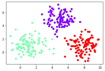
233 |
234 |
235 | ### CHOOSING VALUE OF K
236 |
237 | While working with the k-means clustering scratch, one thing we must keep in mind is the number of clusters ‘k’. We should make sure that we are choosing the optimum number of clusters for the given data set. But, here arises a question, how to choose the optimum value of k ?? We use the elbow method which is generally used in analyzing the optimum value of k.
238 |
239 | The Elbow method is based on the principle that **“Sum of squares of distances of every data point from its corresponding cluster centroid should be as minimum as possible”. **
240 |
241 | ### STEPS OF CHOOSING BEST K VALUE
242 |
243 | - Run k-means clustering model on various values of k
244 | - For each value of K, calculate the Sum of squares of distances of every data point from its corresponding cluster centroid which is called WCSS ( Within-Cluster Sums of Squares)
245 | - Plot the value of WCSS with respect to various values of K
246 | - To select the value of k, we choose the value where there is bend (knee) on the plot i.e. WCSS isn’t increasing rapidly.
247 |
248 | 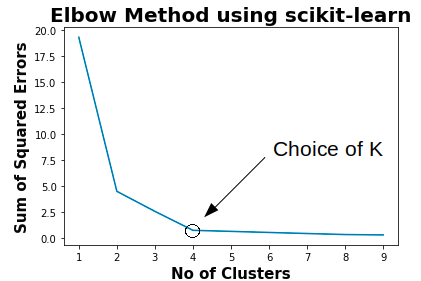
249 |
250 | ### PROS OF K-MEANS
251 | - Relatively simple to learn and understand as the algorithm solely depends on the euclidean method of distance calculation.
252 | - K means works on minimizing Sum of squares of distances, hence it guarantees convergence
253 | - Computational cost is O(K*n*d), hence K means is fast and efficient
254 |
255 |
256 | ### CONS OF K-MEANS
257 | - Difficulty in choosing the optimum number of clusters K
258 | - K means has a problem when clusters are of different size, densities, and non-globular shapes
259 | - K means has problems when data contains outliers
260 | - As the number of dimensions increases, the difficulty in getting the algorithm to converge increases due to the curse of dimensionality
261 | - If there is overlapping between clusters, k-means doesn’t have an intrinsic measure for uncertainty
262 |
--------------------------------------------------------------------------------
/ML from Scratch/Logistic Regression/README.md:
--------------------------------------------------------------------------------
1 | # LOGISTIC REGRESSION FROM SCRATCH
2 | 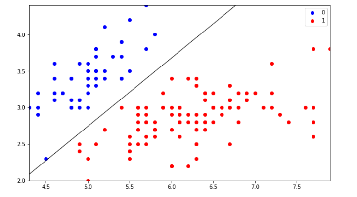
3 |
4 | Before begin, let's assume you are already familar with some of the following topics:
5 |
6 | * Classification and Regression in Machine Learning
7 | * Binary Classification and Multi-class classification
8 | * Basic Geometry of Line, Plane, and Hyper-Plane in 2D, 3D, and n-D space respectively
9 | * Maxima and Minima
10 | * Loss Function
11 |
12 | ## 1. WHAT IS LOGISTIC REGRESSION?
13 |
14 | In simple Terms, Logistic Regression is a Classification technique, which is best used for Binary Classification Problems. Logistic regression is used to describe data and to explain the relationship between one dependent binary variable and one or more independent variables.
15 |
16 | Let’s say, we have a Binary Classification problem, which has only 2 classes true or false. Imagine we want to detect whether a credit card transaction is genuine or fraudulent.
17 |
18 | `+1 = Genuine & -1 = Fraudulent`
19 |
20 | Firstly, let’s try to plot our data points in a 2D space, considering we can visualize 2D in a better way here.
21 |
22 | 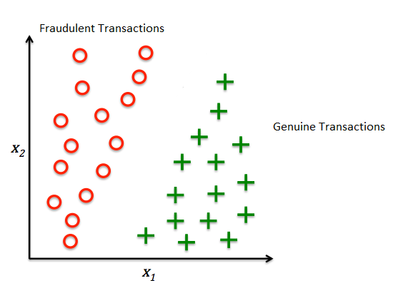
23 |
24 | ### 1.1 HOW DO WE DIFFERENTIATE DATA POINTS ?
25 |
26 | As a human being, if we show this image to a little child with no knowledge of Maths or graph and ask them to differentiate between the two points, I am pretty much sure that he will use his common sense and will draw a line in-between the two points which will differentiate them. That line is called a Decision Boundary, as shown below:
27 |
28 | 
29 |
30 | Anything on the left side of the boundary is Fraudulent and anything on the right side of the boundary is Genuine. This is a common-sense approach.
31 |
32 | ### 1.2. HOW TO BUILD BOUNDARY?
33 |
34 | Now, if we look at it from a Geometric perspective, then the decision boundary is nothing but a simple Line in 2D space. And we know that line also has an equation that can be used to represent it. Now a line can be represented using 2 unique variables, `“m”` and `“b”`:
35 |
36 | In two dimensions, the equation for non-vertical lines is often given in the slope-intercept form: `y = mx + b` where:
37 |
38 | m is the slope or gradient of the line.
39 | b is the y-intercept of the line.
40 | x is the independent variable of the function y = f(x).
41 |
42 | If, our line passes through origin then b = 0, then y = mx
43 |
44 | In 3D space we have equation of Plane as:
45 |
46 | `Ax + By + Cz = D`
47 |
48 | If line passes through origin `D=0`, then $ Z = (-)\frac{a}{c}*x + (-)\frac{b}{c} * y$
49 |
50 | Now, this is about 2D and 3D space, in n-D space we have Hyper-Plane instead of Line or Plane.
51 |
52 | ### 1.3. HOW DO WE REPRESENT HYPERPLANE IN EQUATION ?
53 |
54 | Before diving into the topic, a question may arise in your mind: What is a hyperplane? In a concise term, a hyperplane is a decision boundary that helps classify the data points.
55 |
56 | Let us consider a line with multiple points on it.
57 |
58 | For example: If we want to divide a line into two parts such as some points lie on one side and remaining on the other side, we can choose a point as reference.
59 |
60 | So for a line a point is hyperplane.
61 |
62 | For next example, lets take a wall (2D) . If we want to partition it into two parts a single line (1D) can do that.
63 |
64 | Thus if V is an n-dimensional vector space than hyperplane for V is an (n-1)-dimensional subspace.
65 |
66 | **Note: Data points falling on either side of the hyperplane can be attributed to different classes.**
67 |
68 | Let's deep dive into the topic, imagine we have n-dimension in our Hyper-Plane, then each dimension will have its own slope value, let’s call them
69 |
70 | $w_1, w_2, w_3, ........, w_n$
71 |
72 | and let the dimensions we represented as
73 |
74 | $x_1, x_2, x_3, ........, x_n$
75 |
76 | and lets have an intercept term as `“b”`. So, the Hyper-Plane equation holds as:
77 |
78 | $w_1x_1, w_2x_2, w_3x_3, ........, w_nx_n$
79 |
80 | We, can represent it as:
81 |
82 | Mathematically, it is represented as $ b + \Sigma_{i=1}^{0} {w_ix_i} = 0$
83 |
84 | Now, If we consider, $w_i$ as a vector and $x_i$ as another vector, then we can represent ∑$ (w_ix_i)$ as a vector multiplication of 2 different vectors as $w_i^{\ T}x_i$ where $w_i^{\ T}$ is the transposed vector of values represented using all $w_i$ and $x_i$ is the vector represented using all values of $x_i$ . Also, `b` here is a scalar value.
85 |
86 | Considering all these, $w_i$ is normal to our Hyper-Plane then only the multiplication would make sense. This means that `w` is Normal to our Hyper-Plane and as we all know, Normal is always perpendicular to our surface.
87 |
88 | So now, coming back to our model, after all that maths, we conclude that our model needs to learn the Decision Boundary, using 2 important things,
89 |
90 | For simplicity, let’s consider our plane passes through origin. Then `b=0`.
91 |
92 | Now, our model needs to only figure out the values of $w_i$ , which is normal to our Hyper-Plane. The values in our normal is a vector, which means it is a set of values which needs to be found which best suits our data. So the main task in LR boils down to a simple problem of finding a decision boundary, which is a hyperplane, which is represented using ($w_i$ , b) given a Dataset of (+ve, -ve) points that best separate the points.
93 |
94 |
95 | Let’s imagine that $w_i$ is derived, so even after that how are we going to find out the points whether they are of +1 or -1 class. For that let’s consider the below Diagram:
96 |
97 | 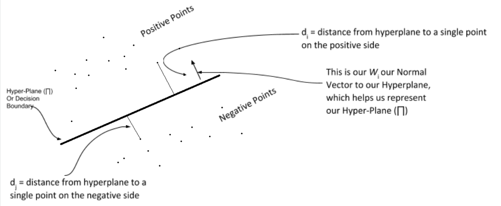
98 |
99 | So, If you know the basics of ML problems, it can be explained as given a set of $x_i$ we have to predict $y_i$. So $y_i$ here belongs to the set {+1, -1}. Now, if we want to calculate the value of $d_i$ or $d_j$ we can do it with the below formula:
100 |
101 | $d_i = \frac{w^{\ T}x_i}{||w||}$
102 |
103 | where w is the normal vector to the out hyperplane, let’s assume that it is Unit Vector for simplicity. Therefore. `||W|| = 1`. Hence, $ \ d_i = w^{\ T}x_i$ and $d_j = w^{\ T}x_j$. Since w and x are on the same side the Hyper-Plane i.e. on the positive side, hence $w^{\ T}x_i$ > 0 and $w^{\ T}x_j$ < 0.
104 |
105 | Basically, it means $d_i$ belongs to +1 class and $d_j$ belongs to -1 class. And, this is how we can classify our data points using the Hyper-Plane.
106 |
107 | ### 1.4. HOW DO WE CALCULATE OUT HYPERPLANE ?
108 |
109 | 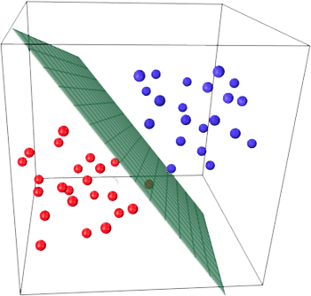
110 |
111 | Well, if you have heard something about optimization problems, our model finds the Hyper-Plane as an optimization problem. Before that, we have to create an optimization equation. Let’s Consider a few cases of $y_i$:
112 |
113 | #### Case 01:
114 | If a point is Positive, and we predict as Positive, then
115 |
116 | $y_i$ = +1 and $w^{\ T}x_i$ = +1, then
117 | $y_i*w^{\ T}x_i$ > 0
118 |
119 | #### Case 02:
120 | If a point is Negative, and we predict as Negative, then
121 |
122 | $y_i$ = -1 and $w^{\ T}x_i$ = -1, then
123 | $y_i*w^{\ T}x_i$ > 0
124 |
125 | #### Case 03:
126 | If a point is Positive, and we predict as Negative, then
127 |
128 | $y_i$ = +1 and $w^{\ T}x_i$ = -1, then
129 | $y_i*w^{\ T}x_i$ < 0
130 |
131 | #### Case 04:
132 | If a point is Negative, and we predict as Positive, then
133 |
134 | $y_i$ = -1 and $w^{\ T}x_i$ = +1, then
135 | $y_i*w^{\ T}x_i$ < 0
136 |
137 | Now, if we look closely whenever we made a correct prediction our equation of $y_i*w^{\ T}x_i$ is always positive, irrespective of the cardinality of our data point. Hence our Optimization equation holds, as such
138 |
139 | (Max w) $\Sigma_{i=1}^{0}(y_i*w^{\ T}x_i$) > 0
140 |
141 | Let’s try to understand what the equation has to offer, the equation says that find me a w (the vector normal to our Hyper-Plane) which has a maximum of $(y_i*w^{\ T}x_i$) > 0 such that the value of `“i”` ranges from `1 to n`, where `“n”` is the total number of dimensions we have.
142 |
143 | It means, for which ever Hyperplane, we have maximum correctly predicted points we will choose that.
144 |
145 | ### 1.5. HOW DO WE SOLVE THE OPTIMIZATION PROBLEM TO FIND THE OPTIMAL W WHICH HAS THE MAX CORRECTLY CLASSIFIED POINT?
146 |
147 | Logistic Regression uses Logistic Function. The logistic function also called the sigmoid function is an S-shaped curve that will take any real-valued number and map it into a worth between 0 and 1, but never exactly at those limits.
148 |
149 | 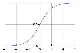
150 |
151 |
152 | $\sigma(t) = \frac{e^t}{e^t + 1} = \frac{1}{1 + e^{-t}}$
153 |
154 | So we use our optimization equation in place of “t”
155 |
156 | t = $y_i*w^{\ T}x_i$ s.t. (i = {1,n})
157 |
158 | And when we solve this sigmoid function, we get another optimization problem, which is computationally easy to solve. The end Optimization equation becomes as below:
159 |
160 | w* = (Argmin w) ∑$log_n(1 + e^{-t})$
161 |
162 | So, our equation changes form finding a Max to Min, now we can solve this using optimizer or a Gradient Descent. Now, to solve this equation we use something like Gradient Descent, intuitively it tries to find the minima of a function. In our case, it tries to find the minima of out sigmoid function.
163 |
164 | ### 1.6 HOW DOES IT MINIMIZE A FUNCTION OR FINDS MINIMA?
165 |
166 | Our Optimizer tries to minimize the loss function of our sigmoid, by loss function I mean, it tries to minimize the error made by our model, and eventually finds a Hyper-Plane which has the lowest error. The loss function has the below equation:
167 |
168 | $[y*log(y_p) + (i - y)*log(1 - y_p)]$
169 |
170 | where,
171 | y = actual class value of a data point
172 | $y_p$ = predicted class value of data point
173 |
174 | And so this is what Logistic Regression is and that is how we get our best Decision Boundary for classification. In broader sense, Logistic Regression tries to find the best decision boundary which best separates the data points of different classes.
175 |
176 | ### 1.7. CODE FROM SCRATCH
177 |
178 | Before that, let’s re-iterate over few key points, so the code could make more sense to us:
179 |
180 | X is a set of data points, with m rows and n dimensions.
181 | y is a set of class which define a class for every data point from X as +1 or -1
182 |
183 | z = $w^{\ T}X_i$
184 | w = Set of values for a vector that forms the Normal to our Hyper-Plane
185 | b = Set of scalars of the intercept term, not required if our Hyper-Plane passes through the origin
186 | $y_p$ = predicted value of Xi, from the sigmoid function
187 |
188 | Intuitively speaking, our model tries to learn from each iteration using something called a learning rate and gradient value, think this as, once we predict the value using the sigmoid function, we get some values of $y_p$ and then we have y.
189 |
190 | We calculate error, and then we try to use the error to predict a new set of `w` values, which we use to repeat the cycle, until we finally find the best value possible.
191 |
192 | In today’s code from scratch, I will be working on Iris dataset. So let’s dive into the code
193 |
194 | ```
195 | %matplotlib inline
196 | import numpy as np
197 | import matplotlib.pyplot as plt
198 | import seaborn as sns
199 | from sklearn import datasets
200 | from sklearn import linear_model
201 |
202 | iris = datasets.load_iris()
203 | X = iris.data[:, :2] #we use only 2 class
204 | y = (iris.target != 0) * 1
205 | ```
206 |
207 | Let’s try to plot and see how our data lies. Whether can it be separated using a decision boundary.
208 |
209 | ```
210 | plt.scatter(X[y == 0][:, 0], X[y == 0][:, 1], color='b', label='0')
211 | plt.scatter(X[y == 1][:, 0], X[y == 1][:, 1], color='r', label='1')
212 | plt.legend();
213 | ```
214 |
215 | 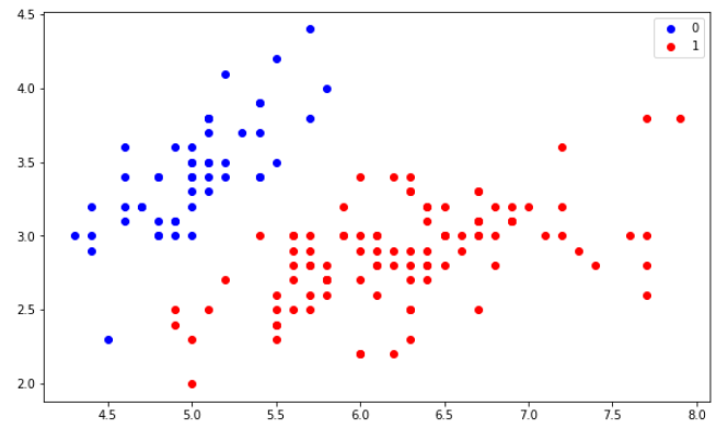
216 |
217 | ```
218 | class LogisticRegression:
219 |
220 | # defining parameters such as learning rate, number ot iterations, whether to include intercept,
221 | # and verbose which says whether to print anything or not like, loss etc.
222 | def __init__(self, learning_rate=0.01, num_iterations=50000, fit_intercept=True, verbose=False):
223 | self.learning_rate = learning_rate
224 | self.num_iterations = num_iterations
225 | self.fit_intercept = fit_intercept
226 | self.verbose = verbose
227 |
228 | # function to define the Incercept value.
229 | def __b_intercept(self, X):
230 | # initially we set it as all 1's
231 | intercept = np.ones((X.shape[0], 1))
232 | # then we concatinate them to the value of X, we don't add we just append them at the end.
233 | return np.concatenate((intercept, X), axis=1)
234 |
235 | def __sigmoid_function(self, z):
236 | # this is our actual sigmoid function which predicts our yp
237 | return 1 / (1 + np.exp(-z))
238 |
239 | def __loss(self, yp, y):
240 | # this is the loss function which we use to minimize the error of our model
241 | return (-y * np.log(yp) - (1 - y) * np.log(1 - yp)).mean()
242 |
243 | # this is the function which trains our model.
244 | def fit(self, X, y):
245 |
246 | # as said if we want our intercept term to be added we use fit_intercept=True
247 | if self.fit_intercept:
248 | X = self.__b_intercept(X)
249 |
250 | # weights initialization of our Normal Vector, initially we set it to 0, then we learn it eventually
251 | self.W = np.zeros(X.shape[1])
252 |
253 | # this for loop runs for the number of iterations provided
254 | for i in range(self.num_iterations):
255 |
256 | # this is our W * Xi
257 | z = np.dot(X, self.W)
258 |
259 | # this is where we predict the values of Y based on W and Xi
260 | yp = self.__sigmoid_function(z)
261 |
262 | # this is where the gradient is calculated form the error generated by our model
263 | gradient = np.dot(X.T, (yp - y)) / y.size
264 |
265 | # this is where we update our values of W, so that we can use the new values for the next iteration
266 | self.W -= self.learning_rate * gradient
267 |
268 | # this is our new W * Xi
269 | z = np.dot(X, self.W)
270 | yp = self.__sigmoid_function(z)
271 |
272 | # this is where the loss is calculated
273 | loss = self.__loss(yp, y)
274 |
275 | # as mentioned above if we want to print somehting we use verbose, so if verbose=True then our loss get printed
276 | if(self.verbose ==True and i % 10000 == 0):
277 | print(f'loss: {loss} \t')
278 |
279 | # this is where we predict the probability values based on out generated W values out of all those iterations.
280 | def predict_prob(self, X):
281 | # as said if we want our intercept term to be added we use fit_intercept=True
282 | if self.fit_intercept:
283 | X = self.__b_intercept(X)
284 |
285 | # this is the final prediction that is generated based on the values learned.
286 | return self.__sigmoid_function(np.dot(X, self.W))
287 |
288 | # this is where we predict the actual values 0 or 1 using round. anything less than 0.5 = 0 or more than 0.5 is 1
289 | def predict(self, X):
290 | return self.predict_prob(X).round()
291 | ```
292 |
293 | Let’s train the model by creating a class of it, we will give Learning rate as 0.1 and number of iterations as 300000.
294 |
295 | ```
296 | model = LogisticRegression(learning_rate=0.1, num_iterations=300000)
297 | model.fit(X, y)
298 | ```
299 |
300 | Lets us see how well our prediction works:
301 |
302 | ```
303 | preds = model.predict(X)
304 | (preds == y).mean()
305 |
306 | Output: 1.0
307 | ```
308 |
309 | ```
310 | plt.figure(figsize=(10, 6))
311 | plt.scatter(X[y == 0][:, 0], X[y == 0][:, 1], color='b', label='0')
312 | plt.scatter(X[y == 1][:, 0], X[y == 1][:, 1], color='r', label='1')
313 | plt.legend()
314 | x1_min, x1_max = X[:,0].min(), X[:,0].max(),
315 | x2_min, x2_max = X[:,1].min(), X[:,1].max(),
316 | xx1, xx2 = np.meshgrid(np.linspace(x1_min, x1_max), np.linspace(x2_min, x2_max))
317 | grid = np.c_[xx1.ravel(), xx2.ravel()]
318 | probs = model.predict_prob(grid).reshape(xx1.shape)
319 | plt.contour(xx1, xx2, probs, [0.5], linewidths=1, colors='black');
320 | ```
321 |
322 | ### 1.8. LOGISTIC REGRESSION FROM SCIKIT LEARN
323 |
324 | ```
325 | from sklearn.linear_model import LogisticRegression
326 | from sklearn.metrics import classification_report, confusion_matrix
327 | model = LogisticRegression(solver='liblinear', random_state=0)
328 | model.fit(X, y)
329 | model.predict_proba(X)
330 | ```
331 |
332 | ```
333 | cm = confusion_matrix(y, model.predict(X))
334 |
335 | fig, ax = plt.subplots(figsize=(8, 8))
336 | ax.imshow(cm)
337 | ax.grid(False)
338 | ax.xaxis.set(ticks=(0, 1), ticklabels=('Predicted 0s', 'Predicted 1s'))
339 | ax.yaxis.set(ticks=(0, 1), ticklabels=('Actual 0s', 'Actual 1s'))
340 | ax.set_ylim(1.5, -0.5)
341 | for i in range(2):
342 | for j in range(2):
343 | ax.text(j, i, cm[i, j], ha='center', va='center', color='white')
344 | plt.show()
345 | ```
346 |
347 | ```
348 | print(classification_report(y, model.predict(X)))
349 | ```
350 |
--------------------------------------------------------------------------------
/ML from Scratch/Linear Regression/Predict-Salary-based-on-Experience---Linear-Regression.ipynb:
--------------------------------------------------------------------------------
1 | {
2 | "cells": [
3 | {
4 | "cell_type": "code",
5 | "execution_count": 2,
6 | "metadata": {},
7 | "outputs": [
8 | {
9 | "name": "stdout",
10 | "output_type": "stream",
11 | "text": [
12 | "(30, 2)\n"
13 | ]
14 | },
15 | {
16 | "data": {
17 | "text/html": [
18 | "
 3 |
4 | Artificial intelligence can be interpreted as adding human intelligence in a machine. Artificial intelligence is not a system but a discipline that focuses on making machine smart enough to tackle the problem like the human brain does. The ability to learn, understand, imagine are the qualities that are naturally found in Humans. Developing a system that has the same or better level of these qualities artificially is termed as Artificial Intelligence.
5 |
6 | Machine Learning is a subset of AI. That is, all machine learning counts as AI, but not all AI counts as machine learning. Machine learning refers to the system that can learn by themselves. **Machine learning is the study of computer algorithms that comprises of algorithms and statistical models that allow computer programs to automatically improve through experience.**
7 |
8 | > “Machine learning is the tendency of machines to learn from data analysis and achieve Artificial Intelligence.”
9 |
10 | **Machine Learning** is the science of getting computers to act by feeding them data and letting them learn a few tricks on their own without being explicitly programmed.
11 |
12 | ## DIFFERENCE BETWEEN MACHINE LEARNING AND ARTIFICIAL INTELLIGENCE
13 | * Artificial intelligence focuses on Success whereas Machine Learning focuses on Accuracy
14 | * AI is not a system, but it can be implemented on system to make system intelligent. ML is a system that can extract knowledge from datasets
15 | * AI is used in decision making whereas ML is used in learning from experience
16 | * AI mimics human whereas ML develops self-learning algorithm
17 | * AI leads to wisdom or intelligence whereas ML leads to knowledge or experience
18 | * Machine Learning is one of the way to achieve Artificial Intelligence.
19 |
20 | ## TYPES OF MACHINE LEARNING
21 | * Supervised Learning
22 | * Unsupervised learning
23 | * Reinforced Learning
24 |
25 | **Supervised** means to oversee or direct a certain activity and make sure it is done correctly. In this type of learning the machine learns under guidance. So, at school or teachers guided us and taught us similarly in supervised learning machines learn by feeding them label data and explicitly telling them that this is the input and this is exactly how the output must look. So, the teacher, in this case, is the training data.
26 | * Linear Regression
27 | * Logistic Regression
28 | * Support Vector Machine
29 | * Naive Bayes Classifier
30 | * Artificial Neural Networks, etc
31 |
32 | **Unsupervised** means to act without anyone’s supervision or without anybody’s direction. Now, here the data is not labeled. There is no guide and the machine has to figure out the data set given and it has to find hidden patterns in order to make predictions about the output. An example of unsupervised learning is an adult-like you and me. We do not need a guide to help us with our daily activities. We can figure things out on our own without any supervision.
33 | * K-means clustering
34 | * Principal Component Analysis
35 | * Generative Adversarial Networks
36 |
37 | **Reinforcement** means to establish or encourage a pattern of behavior. It is a learning method wherein an agent learns by producing actions and discovers errors or rewards. Once the agent gets trained it gets ready to predict the new data presented to it.
38 |
39 | Let’s say a child is born. What will he do? But after some months or years, he tries to walk. So here he basically follows the hit and trial concept because he is new to the surroundings and the only way to learn is experience. We notice baby stretching and kicking his legs and starts to roll over. Then he starts crawling. He then tries to stand up but he fails in doing so for many attempts. Then the baby will learn to support all his weight when held in a standing position. This is what reinforcement learning is.
40 |
--------------------------------------------------------------------------------
/Machine Learning from Beginner to Advanced/Key terms used in ML.md:
--------------------------------------------------------------------------------
1 | # KEY TERMS USED IN MACHINE LEARNING
2 |
3 | Before starting tutorials on machine learning, we came with an idea of providing a brief definition of key terms used in Machine Learning. These key terms will be regularly used in our coming tutorials on machine learning from scratch and will also be used in further higher courses. So let’s start with the term Machine Learning:
4 |
5 | ## MACHINE LEARNING
6 | Machine learning is the study of computer algorithms that comprises of algorithms and statistical models that allow computer programs to automatically improve through experience. It is the science of getting computers to act by feeding them data and letting them learn a few tricks on their own without being explicitly programmed.
7 |
8 | > TYPES OF MACHINE LEARNING
3 |
4 | Artificial intelligence can be interpreted as adding human intelligence in a machine. Artificial intelligence is not a system but a discipline that focuses on making machine smart enough to tackle the problem like the human brain does. The ability to learn, understand, imagine are the qualities that are naturally found in Humans. Developing a system that has the same or better level of these qualities artificially is termed as Artificial Intelligence.
5 |
6 | Machine Learning is a subset of AI. That is, all machine learning counts as AI, but not all AI counts as machine learning. Machine learning refers to the system that can learn by themselves. **Machine learning is the study of computer algorithms that comprises of algorithms and statistical models that allow computer programs to automatically improve through experience.**
7 |
8 | > “Machine learning is the tendency of machines to learn from data analysis and achieve Artificial Intelligence.”
9 |
10 | **Machine Learning** is the science of getting computers to act by feeding them data and letting them learn a few tricks on their own without being explicitly programmed.
11 |
12 | ## DIFFERENCE BETWEEN MACHINE LEARNING AND ARTIFICIAL INTELLIGENCE
13 | * Artificial intelligence focuses on Success whereas Machine Learning focuses on Accuracy
14 | * AI is not a system, but it can be implemented on system to make system intelligent. ML is a system that can extract knowledge from datasets
15 | * AI is used in decision making whereas ML is used in learning from experience
16 | * AI mimics human whereas ML develops self-learning algorithm
17 | * AI leads to wisdom or intelligence whereas ML leads to knowledge or experience
18 | * Machine Learning is one of the way to achieve Artificial Intelligence.
19 |
20 | ## TYPES OF MACHINE LEARNING
21 | * Supervised Learning
22 | * Unsupervised learning
23 | * Reinforced Learning
24 |
25 | **Supervised** means to oversee or direct a certain activity and make sure it is done correctly. In this type of learning the machine learns under guidance. So, at school or teachers guided us and taught us similarly in supervised learning machines learn by feeding them label data and explicitly telling them that this is the input and this is exactly how the output must look. So, the teacher, in this case, is the training data.
26 | * Linear Regression
27 | * Logistic Regression
28 | * Support Vector Machine
29 | * Naive Bayes Classifier
30 | * Artificial Neural Networks, etc
31 |
32 | **Unsupervised** means to act without anyone’s supervision or without anybody’s direction. Now, here the data is not labeled. There is no guide and the machine has to figure out the data set given and it has to find hidden patterns in order to make predictions about the output. An example of unsupervised learning is an adult-like you and me. We do not need a guide to help us with our daily activities. We can figure things out on our own without any supervision.
33 | * K-means clustering
34 | * Principal Component Analysis
35 | * Generative Adversarial Networks
36 |
37 | **Reinforcement** means to establish or encourage a pattern of behavior. It is a learning method wherein an agent learns by producing actions and discovers errors or rewards. Once the agent gets trained it gets ready to predict the new data presented to it.
38 |
39 | Let’s say a child is born. What will he do? But after some months or years, he tries to walk. So here he basically follows the hit and trial concept because he is new to the surroundings and the only way to learn is experience. We notice baby stretching and kicking his legs and starts to roll over. Then he starts crawling. He then tries to stand up but he fails in doing so for many attempts. Then the baby will learn to support all his weight when held in a standing position. This is what reinforcement learning is.
40 |
--------------------------------------------------------------------------------
/Machine Learning from Beginner to Advanced/Key terms used in ML.md:
--------------------------------------------------------------------------------
1 | # KEY TERMS USED IN MACHINE LEARNING
2 |
3 | Before starting tutorials on machine learning, we came with an idea of providing a brief definition of key terms used in Machine Learning. These key terms will be regularly used in our coming tutorials on machine learning from scratch and will also be used in further higher courses. So let’s start with the term Machine Learning:
4 |
5 | ## MACHINE LEARNING
6 | Machine learning is the study of computer algorithms that comprises of algorithms and statistical models that allow computer programs to automatically improve through experience. It is the science of getting computers to act by feeding them data and letting them learn a few tricks on their own without being explicitly programmed.
7 |
8 | > TYPES OF MACHINE LEARNING  4 |
5 |
6 | Humans are the most intelligent species found on Earth. The ability to learn, understand, imagine are the qualities that are naturally found in Humans. Developing a system that has the same or better level of these qualities artificially is termed as Artificial Intelligence. Before talking about AI hype, let’s go through brief history of AI.
7 |
8 | ## HISTORY
9 |
10 | The beginning of modern AI started when the term “Artificial Intelligence” was coined in 1956, at a conference at Dartmouth College, in Hanover. Government funding and interest increased but expectations exceeded the reality which led to AI Winter from 1974 to 1980. British government started funding again to compete with the Japanese but couldn’t stop the 2nd AI winter which occurred from 1987 to 1993.
11 |
12 | 
13 |
14 | The field has come a very long way in the past decade. The 10s were the hottest AI summer with tech giants like Google, Facebook, Microsoft repeatedly touting AI’s abilities.
15 |
16 | 
17 |
18 | After the development of higher processing power like GPU, TPU in 10s, Deep Learning made huge jumps. Neural networks offered better results than other algorithms when used on the same data. Talking about the achievement because of Deep learning, Alexa and Siri understanding your voice, Spotify, and Netflix recommending what you watch next, Facebook tagging all your friends in a photo automatically are the remarkable one. With the continuous progress in speed, memory capacity, Quantum Computing performance of AI is being enhanced gradually. Simulations that usually take months are available in days, hours, or less.
19 |
20 | ## CURRENT SCENARIO
21 |
22 | Albert Einstein had once said, “The measure of intelligence is the ability to change”. AI, which started in the 1950s, is aimed at creating a machine that can imitate human behavior with great proficiency. And the question is how AI handles things beyond Human’s imagination? Apart from all the achievements so far in the field of AI, expectations are unreasonably high rather than understanding how it works. Most of the Tech leaders excite people with claims that AI will replace humans but the reality is we do not have the ability to create an AI controlling a robot that can peel an orange.
23 |
24 | In recent years, there’s been intense hype about AI but we aren’t even near living up to the public expectation. Self-driving cars and health care are currently the most hyped areas of artificial intelligence, the most challenging and are taking much longer than the optimistic timetables. AI is still in its infancy, but people are expecting amazing advancements in the next few years like in movies.
25 |
26 | Business-oriented companies are brainwashing or stimulating customers by using AI as a marketing term. Companies deploy some small AI project in their products in a commercial setting. Nowadays, AI is being forcefully tagged in consumer products, like AI Fan, AI fridge, and even AI Toilet. The below picture shows the use of “Artificial Intelligence” in marketing and related key terms.
27 |
28 | ## CHANGE YOUR MIND
29 |
30 | AI is gaining more attention among students and researchers. But, people still don’t realize that they can’t become an expert using stuff like PyTorch, TensorFlow etc. Implementing built-in models with frameworks like Keras, Tensorflow, and Scikit is not unique and special, especially, when we are following an online tutorial and simply changing the data to ours. Coming up and understanding the things behind those architectures is extremely hard. We need a full understanding of probability and statistics, information theory, calculus, etc to just grasp the main ideas.
31 |
32 | AI components are made up of mathematically proven methods or implementation which are coded to work on data. The use of AI depends upon the type of problems they are designed to work on. If ML doesn’t work for you, it’s because you’re not using it right, not because the methods are wrong.
33 |
34 | A routine job that doesn’t require a brain is sure to be replaced by AI. It’s not going to close the job opportunity but will open the different sets of skilled jobs. Let’s take an example of self-driving cars. General Motors, Google’s Waymo, Toyota, Honda, and Tesla are making self-driving cars. After its success, drivers’ jobs will disappear but new job roles of creating and maintaining them will open. Humanity has to evolve towards being more intelligent and it’s the right time.
35 |
36 |
37 | ## CONCLUSION
38 |
39 | We currently call AI as Big Data & Machine Learning. We are focused on finding patterns and predicting the near future trends but AI completely fails when it comes to generating explanations. Reality is, we can’t still trust the decisions of AI in highly-valued & highly-risked domains like finance, healthcare, and energy where even 0.01% accuracy matters.
40 |
41 | With all things taken into consideration, it is sure that AI hype will gradually decrease when people realize we are still using “pseudo-AI” where the fact is humans are operating AI behind the scenes. Though AI has been bookended by fear, doubt, and misinformation, AI hype doesn’t seem to come to an end sooner.
42 |
--------------------------------------------------------------------------------
/ML from Scratch/Linear Regression/README.md:
--------------------------------------------------------------------------------
1 | # LINEAR REGRESSION FROM SCRATCH
2 |
3 | 
4 |
5 | Regression is the method which measures the average relationship between two or more continuous variables in term of the response variable and feature variables. In other words, regression analysis is to know the nature of the relationship between two or more variables to use it for predicting the most likely value of dependent variables for a given value of independent variables. Linear regression is a mostly used regression algorithm.
6 |
7 | For more concrete understanding, let’s say there is a high correlation between day temperature and sales of tea and coffee. Then the salesman might wish to know the temperature for the next day to decide for the stock of tea and coffee. This can be done with the help of regression.
8 |
9 | The variable, whose value is estimated, predicted, or influenced is called a dependent variable. And the variable which is used for prediction or is known is called an independent variable. It is also called explanatory, regressor, or predictor variable.
10 |
11 | ## 1. LINEAR REGRESSION
12 |
13 | Linear Regression is a supervised method that tries to find a relation between a continuous set of variables from any given dataset. So, the problem statement that the algorithm tries to solve linearly is to best fit a line/plane/hyperplane (as the dimension goes on increasing) for any given set of data.
14 |
15 | This algorithm use statistics on the training data to find the best fit linear or straight-line relationship between the input variables (X) and output variable (y). Simple equation of Linear Regression model can be written as:
16 |
17 | ```
18 | Y=mX+c ; Here m and c are calculated on training
19 | ```
20 |
21 | In the above equation, m is the scale factor or coefficient, c being the bias coefficient, Y is the dependent variable and X is the independent variable. Once the coefficient m and c are known, this equation can be used to predict the output value Y when input X is provided.
22 |
23 | Mathematically, coefficients m and c can be calculated as:
24 |
25 | ```
26 | m = sum((X(i) - mean(X)) * (Y(i) - mean(Y))) / sum( (X(i) - mean(X))^2)
27 | c = mean(Y) - m * mean(X)
28 | ```
29 | 
30 |
31 | As you can see, the red point is very near the regression line; its error of prediction is small. By contrast, the yellow point is much higher than the regression line and therefore its error of prediction is large. The best-fitting line is the line that minimizes the sum of the squared errors of prediction.
32 |
33 | ## 1.1. LINEAR REGRESSION FROM SCRATCH
34 |
35 | We will build a linear regression model to predict the salary of a person on the basis of years of experience from scratch. You can download the dataset from the link given below. Let’s start with importing required libraries:
36 |
37 | ```
38 | %matplotlib inline
39 | import numpy as np
40 | import matplotlib.pyplot as plt
41 | import pandas as pd
42 | ```
43 |
44 | We are using dataset of 30 data items consisting of features like years of experience and salary. Let’s visualize the dataset first.
45 |
46 | ```
47 | dataset = pd.read_csv('salaries.csv')
48 |
49 | #Scatter Plot
50 | X = dataset['Years of Experience']
51 | Y = dataset['Salary']
52 |
53 | plt.scatter(X,Y,color='blue')
54 | plt.xlabel('Years of Experience')
55 | plt.ylabel('Salary')
56 | plt.title('Salary Prediction Curves')
57 | plt.show()
58 | ```
59 | 
60 |
61 | ```
62 | def mean(values):
63 | return sum(values) / float(len(values))
64 |
65 | # initializing our inputs and outputs
66 | X = dataset['Years of Experience'].values
67 | Y = dataset['Salary'].values
68 |
69 | # mean of our inputs and outputs
70 | x_mean = mean(X)
71 | y_mean = mean(Y)
72 |
73 | #total number of values
74 | n = len(X)
75 |
76 | # using the formula to calculate the b1 and b0
77 | numerator = 0
78 | denominator = 0
79 | for i in range(n):
80 | numerator += (X[i] - x_mean) * (Y[i] - y_mean)
81 | denominator += (X[i] - x_mean) ** 2
82 |
83 | b1 = numerator / denominator
84 | b0 = y_mean - (b1 * x_mean)
85 |
86 | #printing the coefficient
87 | print(b1, b0)
88 | ```
89 | Finally, we have calculated the unknown coefficient m as b1 and c as b0. Here we have b1 = **9449.962321455077** and b0 = **25792.20019866869**.
90 |
91 | Let’s visualize the best fit line from scratch.
92 |
93 | 
94 |
95 | Now let’s predict the salary Y by providing years of experience as X:
96 |
97 | ```
98 | def predict(x):
99 | return (b0 + b1 * x)
100 | y_pred = predict(6.5)
101 | print(y_pred)
102 |
103 | Output: 87216.95528812669
104 | ```
105 | ### 1.2. LINEAR REGRESSION USING SKLEARN
106 |
107 | ```
108 | from sklearn.linear_model import LinearRegression
109 |
110 | X = dataset.drop(['Salary'],axis=1)
111 | Y = dataset['Salary']
112 |
113 | reg = LinearRegression() #creating object reg
114 | reg.fit(X,Y) # Fitting the Data set
115 | ```
116 |
117 | Let’s visualize the best fit line using Linear Regression from sklearn
118 |
119 | 
120 |
121 | Now let’s predict the salary Y by providing years of experience as X:
122 |
123 | ```
124 | y_pred = reg.predict([[6.5]])
125 | y_pred
126 |
127 | Output: 87216.95528812669
128 | ```
129 |
130 | ## 1.3. CONCLUSION
131 |
132 | We need to able to measure how good our model is (accuracy). There are many methods to achieve this but we would implement Root mean squared error and coefficient of Determination (R² Score).
133 |
134 | * Try Model with Different error metric for Linear Regression like Mean Absolute Error, Root mean squared error.
135 | * Try algorithm with large data set, imbalanced & balanced dataset so that you can have all flavors of Regression.
136 |
137 |
--------------------------------------------------------------------------------
/Machine Learning from Beginner to Advanced/mathematics_ai_ml_history_motivation.md:
--------------------------------------------------------------------------------
1 | ## HISTORY OF MATHEMATICS
2 |
3 | * ...........?
4 | * Number system: **2500 Years ago**
5 | * 0 1 2 3 4 5 6 7 8 9
6 | * 0 1 2 3 4 5 6 7 8 9 A B
7 | * 0 1
8 |
9 | * Logical Reasoning: Language and Logics
10 | * If **A**, then **B** (if $x^2$ is even, then x is even)
11 | * if not **B**, then not **A** (If x is not even, then $x^2$ is not even)
12 | * Euclidean Algorithm: **2000 years ago**
13 | * **The Elements**: The most influential book of all-time
14 | * Greatest Common Divisor of 2 numbers: **GCD(1054, 714)**
15 | * **Cryptography** (Encryption and Decryption)
16 | * $\pi$ and Geometry (About $5^{th}$ Century)
17 | * Pythagoras Theorem
18 | * Metcalfe's Law
19 | * Suppose, Weight of network is $n^2$ then,
20 | * **Network of 50M = Network of 40M + Network of 30M**
21 | * Input Analysis
22 | * Some programs with n inputs take $n^2$ time to run (Bubble Sort). In terms of processing time: **50 inputs = 40 inputs + 30 inputs**
23 | * Surface Area
24 | * **Area of radius 50 = Area of radius 40 + Area of radius 30**
25 | * Physics
26 | * The KE of an object with mass(m) and velocity(v) is **$1/2mv^2$**. In terms of energy:
27 | * **Energy at 500 mph = Energy at 400 mph + Energy at 300 mph**
28 | * With the energy used to accelerate one bullet to 500 mph, we could accelerate two others to 400 mph and 300 mph
29 | * Logarithms and Algebra
30 | | | Logarithms = Time| Exponents = Growth |
31 | |-|:------------------:|:--------------------:|
32 | |Time/ Growth Perspective| $ln(x)$
4 |
5 |
6 | Humans are the most intelligent species found on Earth. The ability to learn, understand, imagine are the qualities that are naturally found in Humans. Developing a system that has the same or better level of these qualities artificially is termed as Artificial Intelligence. Before talking about AI hype, let’s go through brief history of AI.
7 |
8 | ## HISTORY
9 |
10 | The beginning of modern AI started when the term “Artificial Intelligence” was coined in 1956, at a conference at Dartmouth College, in Hanover. Government funding and interest increased but expectations exceeded the reality which led to AI Winter from 1974 to 1980. British government started funding again to compete with the Japanese but couldn’t stop the 2nd AI winter which occurred from 1987 to 1993.
11 |
12 | 
13 |
14 | The field has come a very long way in the past decade. The 10s were the hottest AI summer with tech giants like Google, Facebook, Microsoft repeatedly touting AI’s abilities.
15 |
16 | 
17 |
18 | After the development of higher processing power like GPU, TPU in 10s, Deep Learning made huge jumps. Neural networks offered better results than other algorithms when used on the same data. Talking about the achievement because of Deep learning, Alexa and Siri understanding your voice, Spotify, and Netflix recommending what you watch next, Facebook tagging all your friends in a photo automatically are the remarkable one. With the continuous progress in speed, memory capacity, Quantum Computing performance of AI is being enhanced gradually. Simulations that usually take months are available in days, hours, or less.
19 |
20 | ## CURRENT SCENARIO
21 |
22 | Albert Einstein had once said, “The measure of intelligence is the ability to change”. AI, which started in the 1950s, is aimed at creating a machine that can imitate human behavior with great proficiency. And the question is how AI handles things beyond Human’s imagination? Apart from all the achievements so far in the field of AI, expectations are unreasonably high rather than understanding how it works. Most of the Tech leaders excite people with claims that AI will replace humans but the reality is we do not have the ability to create an AI controlling a robot that can peel an orange.
23 |
24 | In recent years, there’s been intense hype about AI but we aren’t even near living up to the public expectation. Self-driving cars and health care are currently the most hyped areas of artificial intelligence, the most challenging and are taking much longer than the optimistic timetables. AI is still in its infancy, but people are expecting amazing advancements in the next few years like in movies.
25 |
26 | Business-oriented companies are brainwashing or stimulating customers by using AI as a marketing term. Companies deploy some small AI project in their products in a commercial setting. Nowadays, AI is being forcefully tagged in consumer products, like AI Fan, AI fridge, and even AI Toilet. The below picture shows the use of “Artificial Intelligence” in marketing and related key terms.
27 |
28 | ## CHANGE YOUR MIND
29 |
30 | AI is gaining more attention among students and researchers. But, people still don’t realize that they can’t become an expert using stuff like PyTorch, TensorFlow etc. Implementing built-in models with frameworks like Keras, Tensorflow, and Scikit is not unique and special, especially, when we are following an online tutorial and simply changing the data to ours. Coming up and understanding the things behind those architectures is extremely hard. We need a full understanding of probability and statistics, information theory, calculus, etc to just grasp the main ideas.
31 |
32 | AI components are made up of mathematically proven methods or implementation which are coded to work on data. The use of AI depends upon the type of problems they are designed to work on. If ML doesn’t work for you, it’s because you’re not using it right, not because the methods are wrong.
33 |
34 | A routine job that doesn’t require a brain is sure to be replaced by AI. It’s not going to close the job opportunity but will open the different sets of skilled jobs. Let’s take an example of self-driving cars. General Motors, Google’s Waymo, Toyota, Honda, and Tesla are making self-driving cars. After its success, drivers’ jobs will disappear but new job roles of creating and maintaining them will open. Humanity has to evolve towards being more intelligent and it’s the right time.
35 |
36 |
37 | ## CONCLUSION
38 |
39 | We currently call AI as Big Data & Machine Learning. We are focused on finding patterns and predicting the near future trends but AI completely fails when it comes to generating explanations. Reality is, we can’t still trust the decisions of AI in highly-valued & highly-risked domains like finance, healthcare, and energy where even 0.01% accuracy matters.
40 |
41 | With all things taken into consideration, it is sure that AI hype will gradually decrease when people realize we are still using “pseudo-AI” where the fact is humans are operating AI behind the scenes. Though AI has been bookended by fear, doubt, and misinformation, AI hype doesn’t seem to come to an end sooner.
42 |
--------------------------------------------------------------------------------
/ML from Scratch/Linear Regression/README.md:
--------------------------------------------------------------------------------
1 | # LINEAR REGRESSION FROM SCRATCH
2 |
3 | 
4 |
5 | Regression is the method which measures the average relationship between two or more continuous variables in term of the response variable and feature variables. In other words, regression analysis is to know the nature of the relationship between two or more variables to use it for predicting the most likely value of dependent variables for a given value of independent variables. Linear regression is a mostly used regression algorithm.
6 |
7 | For more concrete understanding, let’s say there is a high correlation between day temperature and sales of tea and coffee. Then the salesman might wish to know the temperature for the next day to decide for the stock of tea and coffee. This can be done with the help of regression.
8 |
9 | The variable, whose value is estimated, predicted, or influenced is called a dependent variable. And the variable which is used for prediction or is known is called an independent variable. It is also called explanatory, regressor, or predictor variable.
10 |
11 | ## 1. LINEAR REGRESSION
12 |
13 | Linear Regression is a supervised method that tries to find a relation between a continuous set of variables from any given dataset. So, the problem statement that the algorithm tries to solve linearly is to best fit a line/plane/hyperplane (as the dimension goes on increasing) for any given set of data.
14 |
15 | This algorithm use statistics on the training data to find the best fit linear or straight-line relationship between the input variables (X) and output variable (y). Simple equation of Linear Regression model can be written as:
16 |
17 | ```
18 | Y=mX+c ; Here m and c are calculated on training
19 | ```
20 |
21 | In the above equation, m is the scale factor or coefficient, c being the bias coefficient, Y is the dependent variable and X is the independent variable. Once the coefficient m and c are known, this equation can be used to predict the output value Y when input X is provided.
22 |
23 | Mathematically, coefficients m and c can be calculated as:
24 |
25 | ```
26 | m = sum((X(i) - mean(X)) * (Y(i) - mean(Y))) / sum( (X(i) - mean(X))^2)
27 | c = mean(Y) - m * mean(X)
28 | ```
29 | 
30 |
31 | As you can see, the red point is very near the regression line; its error of prediction is small. By contrast, the yellow point is much higher than the regression line and therefore its error of prediction is large. The best-fitting line is the line that minimizes the sum of the squared errors of prediction.
32 |
33 | ## 1.1. LINEAR REGRESSION FROM SCRATCH
34 |
35 | We will build a linear regression model to predict the salary of a person on the basis of years of experience from scratch. You can download the dataset from the link given below. Let’s start with importing required libraries:
36 |
37 | ```
38 | %matplotlib inline
39 | import numpy as np
40 | import matplotlib.pyplot as plt
41 | import pandas as pd
42 | ```
43 |
44 | We are using dataset of 30 data items consisting of features like years of experience and salary. Let’s visualize the dataset first.
45 |
46 | ```
47 | dataset = pd.read_csv('salaries.csv')
48 |
49 | #Scatter Plot
50 | X = dataset['Years of Experience']
51 | Y = dataset['Salary']
52 |
53 | plt.scatter(X,Y,color='blue')
54 | plt.xlabel('Years of Experience')
55 | plt.ylabel('Salary')
56 | plt.title('Salary Prediction Curves')
57 | plt.show()
58 | ```
59 | 
60 |
61 | ```
62 | def mean(values):
63 | return sum(values) / float(len(values))
64 |
65 | # initializing our inputs and outputs
66 | X = dataset['Years of Experience'].values
67 | Y = dataset['Salary'].values
68 |
69 | # mean of our inputs and outputs
70 | x_mean = mean(X)
71 | y_mean = mean(Y)
72 |
73 | #total number of values
74 | n = len(X)
75 |
76 | # using the formula to calculate the b1 and b0
77 | numerator = 0
78 | denominator = 0
79 | for i in range(n):
80 | numerator += (X[i] - x_mean) * (Y[i] - y_mean)
81 | denominator += (X[i] - x_mean) ** 2
82 |
83 | b1 = numerator / denominator
84 | b0 = y_mean - (b1 * x_mean)
85 |
86 | #printing the coefficient
87 | print(b1, b0)
88 | ```
89 | Finally, we have calculated the unknown coefficient m as b1 and c as b0. Here we have b1 = **9449.962321455077** and b0 = **25792.20019866869**.
90 |
91 | Let’s visualize the best fit line from scratch.
92 |
93 | 
94 |
95 | Now let’s predict the salary Y by providing years of experience as X:
96 |
97 | ```
98 | def predict(x):
99 | return (b0 + b1 * x)
100 | y_pred = predict(6.5)
101 | print(y_pred)
102 |
103 | Output: 87216.95528812669
104 | ```
105 | ### 1.2. LINEAR REGRESSION USING SKLEARN
106 |
107 | ```
108 | from sklearn.linear_model import LinearRegression
109 |
110 | X = dataset.drop(['Salary'],axis=1)
111 | Y = dataset['Salary']
112 |
113 | reg = LinearRegression() #creating object reg
114 | reg.fit(X,Y) # Fitting the Data set
115 | ```
116 |
117 | Let’s visualize the best fit line using Linear Regression from sklearn
118 |
119 | 
120 |
121 | Now let’s predict the salary Y by providing years of experience as X:
122 |
123 | ```
124 | y_pred = reg.predict([[6.5]])
125 | y_pred
126 |
127 | Output: 87216.95528812669
128 | ```
129 |
130 | ## 1.3. CONCLUSION
131 |
132 | We need to able to measure how good our model is (accuracy). There are many methods to achieve this but we would implement Root mean squared error and coefficient of Determination (R² Score).
133 |
134 | * Try Model with Different error metric for Linear Regression like Mean Absolute Error, Root mean squared error.
135 | * Try algorithm with large data set, imbalanced & balanced dataset so that you can have all flavors of Regression.
136 |
137 |
--------------------------------------------------------------------------------
/Machine Learning from Beginner to Advanced/mathematics_ai_ml_history_motivation.md:
--------------------------------------------------------------------------------
1 | ## HISTORY OF MATHEMATICS
2 |
3 | * ...........?
4 | * Number system: **2500 Years ago**
5 | * 0 1 2 3 4 5 6 7 8 9
6 | * 0 1 2 3 4 5 6 7 8 9 A B
7 | * 0 1
8 |
9 | * Logical Reasoning: Language and Logics
10 | * If **A**, then **B** (if $x^2$ is even, then x is even)
11 | * if not **B**, then not **A** (If x is not even, then $x^2$ is not even)
12 | * Euclidean Algorithm: **2000 years ago**
13 | * **The Elements**: The most influential book of all-time
14 | * Greatest Common Divisor of 2 numbers: **GCD(1054, 714)**
15 | * **Cryptography** (Encryption and Decryption)
16 | * $\pi$ and Geometry (About $5^{th}$ Century)
17 | * Pythagoras Theorem
18 | * Metcalfe's Law
19 | * Suppose, Weight of network is $n^2$ then,
20 | * **Network of 50M = Network of 40M + Network of 30M**
21 | * Input Analysis
22 | * Some programs with n inputs take $n^2$ time to run (Bubble Sort). In terms of processing time: **50 inputs = 40 inputs + 30 inputs**
23 | * Surface Area
24 | * **Area of radius 50 = Area of radius 40 + Area of radius 30**
25 | * Physics
26 | * The KE of an object with mass(m) and velocity(v) is **$1/2mv^2$**. In terms of energy:
27 | * **Energy at 500 mph = Energy at 400 mph + Energy at 300 mph**
28 | * With the energy used to accelerate one bullet to 500 mph, we could accelerate two others to 400 mph and 300 mph
29 | * Logarithms and Algebra
30 | | | Logarithms = Time| Exponents = Growth |
31 | |-|:------------------:|:--------------------:|
32 | |Time/ Growth Perspective| $ln(x)$ 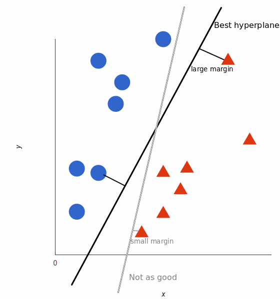 14 |
15 | The line (in 2 input feature) or plane (in 3 input feature) is known as a decision boundary. Every new data from test data will be classified according to this decision boundary. The equation of the hyperplane in the ‘M’ dimension:
16 |
17 | $y = w_0 + w_1x_1 + w_2x_2 + w_3x_3 + ......= w_0 + \Sigma_{i=1}^mw_ix_i = w_0 + w^{T}X = b + w^{T}X $
18 |
19 | where,
14 |
15 | The line (in 2 input feature) or plane (in 3 input feature) is known as a decision boundary. Every new data from test data will be classified according to this decision boundary. The equation of the hyperplane in the ‘M’ dimension:
16 |
17 | $y = w_0 + w_1x_1 + w_2x_2 + w_3x_3 + ......= w_0 + \Sigma_{i=1}^mw_ix_i = w_0 + w^{T}X = b + w^{T}X $
18 |
19 | where, 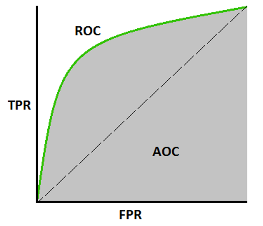 98 |
99 | **Advantages**:
100 | * A simple graphical representation of the diagnostic accuracy of a test: the closer the apex of the curve toward the upper left corner, the greater the discriminatory ability of the test.
101 | * Also, allows a more complex (and more exact) measure of the accuracy of a test, which is the AUC.
102 | * The AUC in turn can be used as a simple numeric rating of diagnostic test accuracy, which simplifies comparison between diagnostic tests.
103 |
104 | **Disadvantages**:
105 | * Actual decision thresholds are usually not displayed in the plot.
106 | * As the sample size decreases, the plot becomes more jagged.
107 | * Not easily interpretable from a business perspective.
108 |
109 | _**So there you have it, some of the widely used performance metrics for Classification Models.**_
110 |
--------------------------------------------------------------------------------
/Installation/install_anaconda_python.md:
--------------------------------------------------------------------------------
1 | # How To Install the Anaconda Python on Windows and Linux (Ubuntu and it's Derivatives)
2 |
3 | Setting up software requirements (environment) is the first and the most important step in getting started with Machine Learning. It takes a lot of effort to get all of those things ready at times. When we finish preparing for the work environment, we will be halfway there.
4 |
5 | In this file, you’ll learn how to use Anaconda to build up a Python machine learning development environment. These instructions are suitable for both Windows and Linux systems.
6 |
7 | * Steps are to install Anaconda in Windows & Ubuntu
8 | * Creating & Working On Conda Environment
9 | * Walkthrough on ML Project
10 |
11 | ## 1. Introduction
12 | Anaconda is an open-source package manager, environment manager, and distribution of the Python and R programming languages. It is used for data science, machine learning, large-scale data processing, scientific computing, and predictive analytics.
13 |
14 | Anaconda aims to simplify package management and deployment. The distribution includes 250 open-source data packages, with over 7,500 more available via the Anaconda repositories suitable for Windows,Linux and MacOS. It also includes the conda command-line tool and a desktop GUI called Anaconda Navigator.
15 |
16 | ### 1.1. Install Anaconda on Windows
17 |
18 | * Go to anaconda official website
19 | * [Download](https://www.anaconda.com/products/distribution) based on your Operating set up (64x or 32x) for windows
20 | * After Anaconda has finished downloading, double-click the _.exe_ file to start the installation process.
21 | * Then, until the installation of Windows is complete, follow the on-screen instructions.
22 | * Don’t forget to add the path to the environmental variable. The benefit is that you can use Anaconda in your Command Prompt, Git Bash, cmder, and so on.
23 | * If you like, you can install Microsoft [VSCode](https://code.visualstudio.com/), but it’s not required.
24 | * Click on Finish
25 | * Open a Command Prompt. If the conda is successfully installed then run conda -V or conda –version in the command prompt and it will pop out the installed version.
26 |
27 | ### 1.2. Install Anaconda on Ubuntu and it's derivatives
28 |
29 | ```Anaconda3-2022.05-Linux-x86_64.sh``` is the most recent stable version at the time of writing this post. Check the [Downloads page](https://www.anaconda.com/distribution/) to see whether there is a new version of Anaconda for Python 3 available for download before downloading the installation script.
30 |
31 | Downloading the newest Anaconda installer bash script, verifying it, and then running it is the best approach to install Anaconda. To install Anaconda on Ubuntu, follow the steps below:
32 |
33 | #### Step 01
34 |
35 | Install the following packages if you’re installing Anaconda on a desktop system and want to use the GUI application.
36 |
37 | ```
38 | $ sudo apt install libgl1-mesa-glx libegl1-mesa libxrandr2 libxrandr2 libxss1 libxcursor1 libxcomposite1 libasound2 libxi6 libxtst6
39 | ```
40 |
41 | #### Step 02
42 |
43 | Download the Anaconda installation script with wget
44 |
45 | ```
46 | $ wget -P /tmp https://repo.anaconda.com/archive/Anaconda3-2022.05-Linux-x86_64.sh
47 | ```
48 |
49 | **_Note_**: If you want to work with different version of anaconda, adjust the [version of anaconda](https://repo.anaconda.com/archive/).
50 |
51 | #### Step 03
52 |
53 | For verifying the data integrity of the installer with cryptographic hash verification you can use the ```SHA-256``` checksum. You’ll use the sha256sum command along with the filename of the script:
54 |
55 | ```
56 | $ sha256sum /tmp/Anaconda3-2022.05-Linux-x86_64.sh`
57 | ```
58 |
59 | You’ll receive output that looks similar to this:
60 |
61 | ```
62 | Output:
63 | afcd2340039557f7b5e8a8a86affa9ddhsdg887jdfifji988686bds
64 | ```
65 |
66 | #### Step 04
67 |
68 | To begin the installation procedure, run the script
69 |
70 | ```
71 | $ bash /tmp/Anaconda3-2022.05-Linux-x86_64.sh
72 | ```
73 |
74 | You’ll receive a welcome mesage as output. Press `ENTER` to continue and then press `ENTER` to read through the license. Once you complete reading the license, you will be asked for approving the license terms.
75 |
76 | ```
77 | Output
78 | Do you approve the license terms? [yes|no]
79 | ```
80 |
81 | Type `yes`.
82 |
83 | Next, you’ll be asked to choose the location of the installation. You can press `ENTER` to accept the default location, or specify a different location to modify it.
84 |
85 | Once you are done you will get a thank you message.
86 |
87 | #### Step 05
88 |
89 | Enter the following bash command to activate the Anaconda installation.
90 |
91 | ```
92 | $ source ~/.bashrc
93 | ```
94 |
95 | Once you have done that, you’ll be placed into the default `base` programming environment of Anaconda, and your command prompt will will show base environment.
96 |
97 | ```
98 | $(base) linus@ubuntu
99 | ```
100 |
101 | ### 1.3. Updating Anaconda
102 |
103 | To update the anaconda to the latest version, open and enter the following command:
104 |
105 | ```
106 | (base) linus@ubuntu:~$ conda update --all -y
107 | ```
108 |
109 | ### 1.4. Creating & Working on Conda Environment
110 |
111 | Anaconda virtual environments let us specify specific package versions. You can specify which version of Python to use for each Anaconda environment you create.
112 |
113 | _**Note**_: Name the environment ```venv_first_env``` or some nice and relevant name as per your project.
114 |
115 | ```
116 | (base) linus@ubuntu:~$ conda create --name venv_first_env python=3.9
117 | ```
118 |
119 | You’ll receive output with information about what is downloaded and which packages will be installed, and then be prompted to proceed with `y` or `n`. As long as you agree, type `y`.
120 |
121 | The `conda` utility will now fetch the packages for the environment and let you know when it’s complete.
122 |
123 | You can activate your new environment by typing the following:
124 |
125 | ```
126 | (base) linus@ubuntu:~$ conda activate venv_first_env
127 | ```
128 |
129 | With your environment activated, your command prompt prefix will reflect that you are no longer in the `base` environment, but in the new one that you just created.
130 |
131 | When you’re ready to deactivate your Anaconda environment, you can do so by typing:
132 |
133 | ```
134 | (venv_first_env) linus@ubuntu:~$ conda deactivate
135 | ```
136 |
137 | With this command, you can see the list of all of the environments you’ve created:
138 |
139 | ```
140 | (base) linus@ubuntu:~$ conda info --envs
141 | ```
142 |
143 | When you create environment using `conda create` , it will come with several default packages. Few examples of then are:
144 |
145 |
146 | - `openssl`
147 | - `pip`
148 | - `python`
149 | - `readline`
150 | - `setuptools`
151 | - `sqlite`
152 | - `tk`
153 |
154 | You might need to add additional package in your environment .
155 |
156 | You can add packages such as `matplotlib` for example, with the following command:
157 |
158 | ```
159 | (venv_first_env) linus@ubuntu:~$ conda install matplotlib
160 | ```
161 |
162 |
163 | For installing the specific version, you can specify specific version with the following command:
164 | ```
165 | (venv_first_env) linus@ubuntu:~$ conda install matplotlib=1.4.3
166 | ```
167 |
168 |
169 | ### 1.5. Getting Started With Jupyter Notebook
170 |
171 | Jupyter Notebooks are capable of performing data visualization in the same environment and are strong, versatile, and shared. Data scientists may use Jupyter Notebooks to generate and distribute documents ranging from code to full-fledged reports.
172 |
173 | You can directly launch Juypter through the terminal using the following command:
174 |
175 | #### Command 01:
176 | ```
177 | (venv_first_env) linus@ubuntu:~$ jupyter notebook
178 | ```
179 |
180 | #### command 02:
181 | ```
182 | (venv_first_env) linus@ubuntu:~$ jupyter notebook --no-browser --port=8885
183 | ```
184 |
185 | ### 06. Working with Jupyter Noteboook
186 |
187 | * create a new notebook, click on the New button on the top right hand corner of the web page and select `Python 3 notebook`. The Python statements are entered in each cell. To execute the Python statements within each cell, press both the `SHIFT` and `ENTER` keys simultaneously. The result will be displayed right below the cell.
188 | * By default, the new notebook will be stored in a file named `Untitled.ipynb`. You can rename the file by clicking on File and Rename menu option at the top
189 | * You can save the notebook by clicking on the `'File'` and `'Save and Checkpoint'` menu options. The notebook will be stored in a file with a `'.ipynb'` extension. You can open the notebook and re-run the program and the results you have saved any time. This powerful feature allows you to share your program and results as well as to reproduce the results generated by others. You can also save the notebook into an HTML format by clicking 'File' followed by 'Download as' options. Note that the IPython notebook is not stored as standard ASCII text files; instead, it is stored in Javascript Object Notation (JSON) file format.
190 |
191 |
98 |
99 | **Advantages**:
100 | * A simple graphical representation of the diagnostic accuracy of a test: the closer the apex of the curve toward the upper left corner, the greater the discriminatory ability of the test.
101 | * Also, allows a more complex (and more exact) measure of the accuracy of a test, which is the AUC.
102 | * The AUC in turn can be used as a simple numeric rating of diagnostic test accuracy, which simplifies comparison between diagnostic tests.
103 |
104 | **Disadvantages**:
105 | * Actual decision thresholds are usually not displayed in the plot.
106 | * As the sample size decreases, the plot becomes more jagged.
107 | * Not easily interpretable from a business perspective.
108 |
109 | _**So there you have it, some of the widely used performance metrics for Classification Models.**_
110 |
--------------------------------------------------------------------------------
/Installation/install_anaconda_python.md:
--------------------------------------------------------------------------------
1 | # How To Install the Anaconda Python on Windows and Linux (Ubuntu and it's Derivatives)
2 |
3 | Setting up software requirements (environment) is the first and the most important step in getting started with Machine Learning. It takes a lot of effort to get all of those things ready at times. When we finish preparing for the work environment, we will be halfway there.
4 |
5 | In this file, you’ll learn how to use Anaconda to build up a Python machine learning development environment. These instructions are suitable for both Windows and Linux systems.
6 |
7 | * Steps are to install Anaconda in Windows & Ubuntu
8 | * Creating & Working On Conda Environment
9 | * Walkthrough on ML Project
10 |
11 | ## 1. Introduction
12 | Anaconda is an open-source package manager, environment manager, and distribution of the Python and R programming languages. It is used for data science, machine learning, large-scale data processing, scientific computing, and predictive analytics.
13 |
14 | Anaconda aims to simplify package management and deployment. The distribution includes 250 open-source data packages, with over 7,500 more available via the Anaconda repositories suitable for Windows,Linux and MacOS. It also includes the conda command-line tool and a desktop GUI called Anaconda Navigator.
15 |
16 | ### 1.1. Install Anaconda on Windows
17 |
18 | * Go to anaconda official website
19 | * [Download](https://www.anaconda.com/products/distribution) based on your Operating set up (64x or 32x) for windows
20 | * After Anaconda has finished downloading, double-click the _.exe_ file to start the installation process.
21 | * Then, until the installation of Windows is complete, follow the on-screen instructions.
22 | * Don’t forget to add the path to the environmental variable. The benefit is that you can use Anaconda in your Command Prompt, Git Bash, cmder, and so on.
23 | * If you like, you can install Microsoft [VSCode](https://code.visualstudio.com/), but it’s not required.
24 | * Click on Finish
25 | * Open a Command Prompt. If the conda is successfully installed then run conda -V or conda –version in the command prompt and it will pop out the installed version.
26 |
27 | ### 1.2. Install Anaconda on Ubuntu and it's derivatives
28 |
29 | ```Anaconda3-2022.05-Linux-x86_64.sh``` is the most recent stable version at the time of writing this post. Check the [Downloads page](https://www.anaconda.com/distribution/) to see whether there is a new version of Anaconda for Python 3 available for download before downloading the installation script.
30 |
31 | Downloading the newest Anaconda installer bash script, verifying it, and then running it is the best approach to install Anaconda. To install Anaconda on Ubuntu, follow the steps below:
32 |
33 | #### Step 01
34 |
35 | Install the following packages if you’re installing Anaconda on a desktop system and want to use the GUI application.
36 |
37 | ```
38 | $ sudo apt install libgl1-mesa-glx libegl1-mesa libxrandr2 libxrandr2 libxss1 libxcursor1 libxcomposite1 libasound2 libxi6 libxtst6
39 | ```
40 |
41 | #### Step 02
42 |
43 | Download the Anaconda installation script with wget
44 |
45 | ```
46 | $ wget -P /tmp https://repo.anaconda.com/archive/Anaconda3-2022.05-Linux-x86_64.sh
47 | ```
48 |
49 | **_Note_**: If you want to work with different version of anaconda, adjust the [version of anaconda](https://repo.anaconda.com/archive/).
50 |
51 | #### Step 03
52 |
53 | For verifying the data integrity of the installer with cryptographic hash verification you can use the ```SHA-256``` checksum. You’ll use the sha256sum command along with the filename of the script:
54 |
55 | ```
56 | $ sha256sum /tmp/Anaconda3-2022.05-Linux-x86_64.sh`
57 | ```
58 |
59 | You’ll receive output that looks similar to this:
60 |
61 | ```
62 | Output:
63 | afcd2340039557f7b5e8a8a86affa9ddhsdg887jdfifji988686bds
64 | ```
65 |
66 | #### Step 04
67 |
68 | To begin the installation procedure, run the script
69 |
70 | ```
71 | $ bash /tmp/Anaconda3-2022.05-Linux-x86_64.sh
72 | ```
73 |
74 | You’ll receive a welcome mesage as output. Press `ENTER` to continue and then press `ENTER` to read through the license. Once you complete reading the license, you will be asked for approving the license terms.
75 |
76 | ```
77 | Output
78 | Do you approve the license terms? [yes|no]
79 | ```
80 |
81 | Type `yes`.
82 |
83 | Next, you’ll be asked to choose the location of the installation. You can press `ENTER` to accept the default location, or specify a different location to modify it.
84 |
85 | Once you are done you will get a thank you message.
86 |
87 | #### Step 05
88 |
89 | Enter the following bash command to activate the Anaconda installation.
90 |
91 | ```
92 | $ source ~/.bashrc
93 | ```
94 |
95 | Once you have done that, you’ll be placed into the default `base` programming environment of Anaconda, and your command prompt will will show base environment.
96 |
97 | ```
98 | $(base) linus@ubuntu
99 | ```
100 |
101 | ### 1.3. Updating Anaconda
102 |
103 | To update the anaconda to the latest version, open and enter the following command:
104 |
105 | ```
106 | (base) linus@ubuntu:~$ conda update --all -y
107 | ```
108 |
109 | ### 1.4. Creating & Working on Conda Environment
110 |
111 | Anaconda virtual environments let us specify specific package versions. You can specify which version of Python to use for each Anaconda environment you create.
112 |
113 | _**Note**_: Name the environment ```venv_first_env``` or some nice and relevant name as per your project.
114 |
115 | ```
116 | (base) linus@ubuntu:~$ conda create --name venv_first_env python=3.9
117 | ```
118 |
119 | You’ll receive output with information about what is downloaded and which packages will be installed, and then be prompted to proceed with `y` or `n`. As long as you agree, type `y`.
120 |
121 | The `conda` utility will now fetch the packages for the environment and let you know when it’s complete.
122 |
123 | You can activate your new environment by typing the following:
124 |
125 | ```
126 | (base) linus@ubuntu:~$ conda activate venv_first_env
127 | ```
128 |
129 | With your environment activated, your command prompt prefix will reflect that you are no longer in the `base` environment, but in the new one that you just created.
130 |
131 | When you’re ready to deactivate your Anaconda environment, you can do so by typing:
132 |
133 | ```
134 | (venv_first_env) linus@ubuntu:~$ conda deactivate
135 | ```
136 |
137 | With this command, you can see the list of all of the environments you’ve created:
138 |
139 | ```
140 | (base) linus@ubuntu:~$ conda info --envs
141 | ```
142 |
143 | When you create environment using `conda create` , it will come with several default packages. Few examples of then are:
144 |
145 |
146 | - `openssl`
147 | - `pip`
148 | - `python`
149 | - `readline`
150 | - `setuptools`
151 | - `sqlite`
152 | - `tk`
153 |
154 | You might need to add additional package in your environment .
155 |
156 | You can add packages such as `matplotlib` for example, with the following command:
157 |
158 | ```
159 | (venv_first_env) linus@ubuntu:~$ conda install matplotlib
160 | ```
161 |
162 |
163 | For installing the specific version, you can specify specific version with the following command:
164 | ```
165 | (venv_first_env) linus@ubuntu:~$ conda install matplotlib=1.4.3
166 | ```
167 |
168 |
169 | ### 1.5. Getting Started With Jupyter Notebook
170 |
171 | Jupyter Notebooks are capable of performing data visualization in the same environment and are strong, versatile, and shared. Data scientists may use Jupyter Notebooks to generate and distribute documents ranging from code to full-fledged reports.
172 |
173 | You can directly launch Juypter through the terminal using the following command:
174 |
175 | #### Command 01:
176 | ```
177 | (venv_first_env) linus@ubuntu:~$ jupyter notebook
178 | ```
179 |
180 | #### command 02:
181 | ```
182 | (venv_first_env) linus@ubuntu:~$ jupyter notebook --no-browser --port=8885
183 | ```
184 |
185 | ### 06. Working with Jupyter Noteboook
186 |
187 | * create a new notebook, click on the New button on the top right hand corner of the web page and select `Python 3 notebook`. The Python statements are entered in each cell. To execute the Python statements within each cell, press both the `SHIFT` and `ENTER` keys simultaneously. The result will be displayed right below the cell.
188 | * By default, the new notebook will be stored in a file named `Untitled.ipynb`. You can rename the file by clicking on File and Rename menu option at the top
189 | * You can save the notebook by clicking on the `'File'` and `'Save and Checkpoint'` menu options. The notebook will be stored in a file with a `'.ipynb'` extension. You can open the notebook and re-run the program and the results you have saved any time. This powerful feature allows you to share your program and results as well as to reproduce the results generated by others. You can also save the notebook into an HTML format by clicking 'File' followed by 'Download as' options. Note that the IPython notebook is not stored as standard ASCII text files; instead, it is stored in Javascript Object Notation (JSON) file format.
190 |
191 |