 4 |
5 | [Gosling.js](https://github.com/gosling-lang/gosling.js) is a declarative grammar for interactive (epi)genomics visualization on the Web.
6 |
7 | ### The Docs and Interactive Tutorials are now hosted at http://gosling-lang.org/
8 |
25 |
26 |
--------------------------------------------------------------------------------
/docs/composition.md:
--------------------------------------------------------------------------------
1 | ---
2 | title: Composition
3 | ---
4 |
5 |
6 | A **track** is a unit building block in Gosling which can be represented as a bar chart, a line chart, or an ideogram. For the concurrent analysis of multiple datasets, multiple tracks can be grouped into **views** and navigated synchronously. In other words, a view defines the genomic location for all the tracks it contains, and the tracks define the data to be visualized.
7 |
8 |
9 |
10 |
11 |
12 |
13 | In Gosling, you can compose multiple tracks and views in diverse ways using the following properties:
14 |
15 | 1. You can display genomic positions of a view either in Cartesian coordinates (**linear**) or in polar coordinates (**circular**) using the `layout` property.
16 | 2. You can determine to either **overlay** or **stack** multiple tracks when composing them into a view using a `alignment` property.
17 | 3. You use juxtapose multiple views in four different ways (i.e., **parallel**, **serial**, **vertical**, **horizontal**) using the `arrangement` property.
18 |
19 | ```javascript
20 | {
21 | "arrangement": "parallel"// how to arrange multiple views
22 | "views": [
23 | {
24 | // a single view can contain multiple tracks
25 | "layout": "circular", // specify the layout of a view
26 | "alignment": "stack", // specify how to align several tracks
27 | "tracks": [
28 | {/** track 1 **/},
29 | {/** track 2 **/},
30 | ...
31 | ]
32 | },
33 | {
34 | /** another view **/
35 | }
36 | ...
37 | ]
38 | }
39 | ```
40 |
41 |
42 | - [Specify the View Layout](#specify-the-view-layout)
43 | - [Align Multiple Tracks in One View](#align-multiple-tracks-in-one-view)
44 | - [Arrange Multiple Views](#arrange-multiple-views)
45 | - [Inherit Property in Nested Structure](#inherit-property-in-nested-structure)
46 |
47 |
48 | ## Specify the View Layout
49 |
50 | In each view, genomic coordinate can be represented in either a **circular** or **linear** layout.
51 |
52 | In the following figure the upper track is using a linear layout while the bottom one is a circular layout.
53 |
54 |
4 |
5 | [Gosling.js](https://github.com/gosling-lang/gosling.js) is a declarative grammar for interactive (epi)genomics visualization on the Web.
6 |
7 | ### The Docs and Interactive Tutorials are now hosted at http://gosling-lang.org/
8 |
25 |
26 |
--------------------------------------------------------------------------------
/docs/composition.md:
--------------------------------------------------------------------------------
1 | ---
2 | title: Composition
3 | ---
4 |
5 |
6 | A **track** is a unit building block in Gosling which can be represented as a bar chart, a line chart, or an ideogram. For the concurrent analysis of multiple datasets, multiple tracks can be grouped into **views** and navigated synchronously. In other words, a view defines the genomic location for all the tracks it contains, and the tracks define the data to be visualized.
7 |
8 |
9 |
10 |
11 |
12 |
13 | In Gosling, you can compose multiple tracks and views in diverse ways using the following properties:
14 |
15 | 1. You can display genomic positions of a view either in Cartesian coordinates (**linear**) or in polar coordinates (**circular**) using the `layout` property.
16 | 2. You can determine to either **overlay** or **stack** multiple tracks when composing them into a view using a `alignment` property.
17 | 3. You use juxtapose multiple views in four different ways (i.e., **parallel**, **serial**, **vertical**, **horizontal**) using the `arrangement` property.
18 |
19 | ```javascript
20 | {
21 | "arrangement": "parallel"// how to arrange multiple views
22 | "views": [
23 | {
24 | // a single view can contain multiple tracks
25 | "layout": "circular", // specify the layout of a view
26 | "alignment": "stack", // specify how to align several tracks
27 | "tracks": [
28 | {/** track 1 **/},
29 | {/** track 2 **/},
30 | ...
31 | ]
32 | },
33 | {
34 | /** another view **/
35 | }
36 | ...
37 | ]
38 | }
39 | ```
40 |
41 |
42 | - [Specify the View Layout](#specify-the-view-layout)
43 | - [Align Multiple Tracks in One View](#align-multiple-tracks-in-one-view)
44 | - [Arrange Multiple Views](#arrange-multiple-views)
45 | - [Inherit Property in Nested Structure](#inherit-property-in-nested-structure)
46 |
47 |
48 | ## Specify the View Layout
49 |
50 | In each view, genomic coordinate can be represented in either a **circular** or **linear** layout.
51 |
52 | In the following figure the upper track is using a linear layout while the bottom one is a circular layout.
53 |
54 | 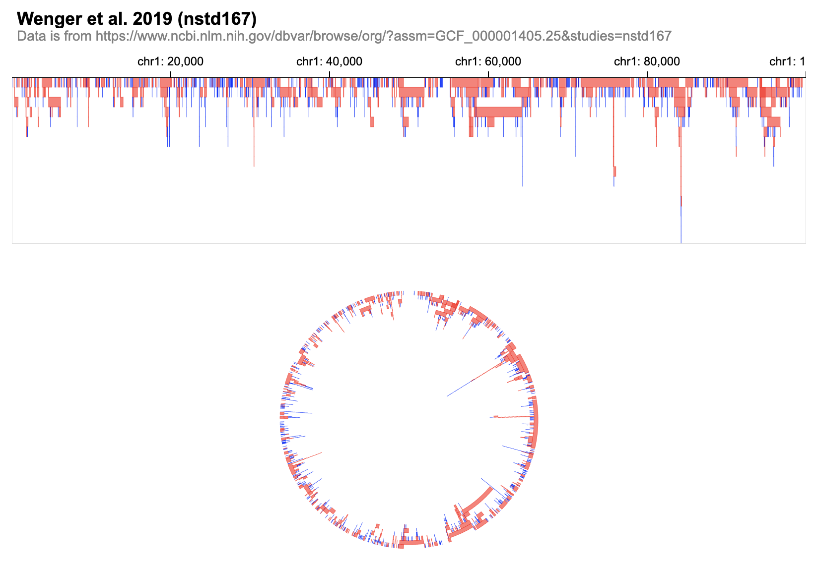 55 |
56 | Users can either specify the layout of all views in the root level
57 |
58 | ```javascript
59 | {
60 | "layout": "linear", //specify the layout of all views
61 | "views":[...]
62 | }
63 | ```
64 |
65 | or specify/override the layout of a certain view in its own definition
66 |
67 | ```javascript
68 | {
69 | "layout": "linear", //specify the layout of all tracks in this view
70 | "tracks":[...]
71 | }
72 | ```
73 |
74 | To enable an easy switch, both `linear` and `circular` layout can be specified through `width` and `height`.
75 | **
55 |
56 | Users can either specify the layout of all views in the root level
57 |
58 | ```javascript
59 | {
60 | "layout": "linear", //specify the layout of all views
61 | "views":[...]
62 | }
63 | ```
64 |
65 | or specify/override the layout of a certain view in its own definition
66 |
67 | ```javascript
68 | {
69 | "layout": "linear", //specify the layout of all tracks in this view
70 | "tracks":[...]
71 | }
72 | ```
73 |
74 | To enable an easy switch, both `linear` and `circular` layout can be specified through `width` and `height`.
75 | **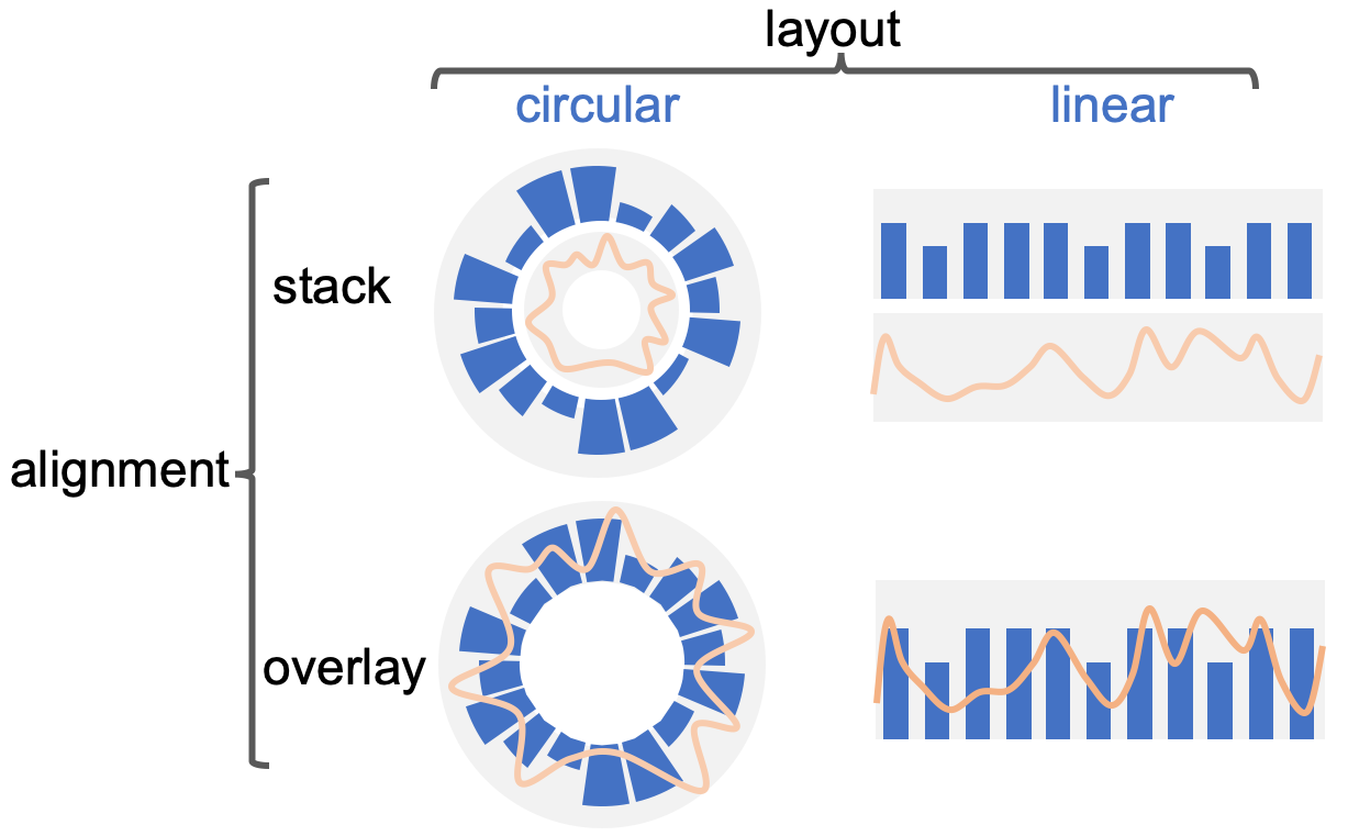 111 |
112 | Multiple `tracks` can compose one single `view`, which has the following properties:
113 |
114 | | property | type | description |
115 | | ------------ | ------- | ------------|
116 | | layout | string | specify the layout type of all tracks, either "linear" or "circular" |
117 | | alignment | string | specify how to align tracks, either "stack" or "overlay". default="stack"|
118 | | spacing | number | specify the space between tracks in pixels (if `layout` is `linear`) or in percentage ranging from `0` to `100` (if `layout` is `circular`) |
119 | | static | boolean | whether to disable [Zooming and Panning](https://github.com/gosling-lang/gosling-docs/blob/master/docs/user-interaction.md#zooming-and-panning), default=false. |
120 | | assembly | string | currently support "hg38", "hg19", "hg18", "hg17", "hg16", "mm10", "mm9" |
121 | | linkingId | string | specify an ID for [linking multiple views](https://github.com/gosling-lang/gosling-docs/blob/master/docs/user-interaction.md#linking-views) |
122 | | centerRadius | number | specify the proportion of the radius of the center white space. A number between [0,1], default=0.3 |
123 | | width | number | required when setting `alignment: overlay` |
124 | | height | number | required when setting `alignment: overlay` |
125 |
126 |
127 |
128 | ## Arrange Multiple Views
129 | Goslings supports multi-view visualizations. How multiple views are arranged is controlled by the `arrangement` property.
130 | ```javascript
131 | {
132 | "arrangement": "parallel",
133 | "views": [
134 | // one view is composed of tracks that share the same layout property (linear or circular)
135 | {
136 | "layout": "linear",
137 | "tracks": [...]
138 | },
139 | // One view can have a hierarchical structure.
140 | // For example, the view below is composed of two sub-views
141 | {
142 | "arrangement": "serial",
143 | "views": [
144 | {
145 | "tracks": [...]
146 | },
147 | {
148 | "tracks": [...]
149 | }
150 | ]
151 | }
152 | ]
153 | }
154 | ```
155 |
156 | Gosling supports four types of arrangemet: `"parallel"`, `"serial"`, `"vertical"`, `"horizontal"`.
157 |
111 |
112 | Multiple `tracks` can compose one single `view`, which has the following properties:
113 |
114 | | property | type | description |
115 | | ------------ | ------- | ------------|
116 | | layout | string | specify the layout type of all tracks, either "linear" or "circular" |
117 | | alignment | string | specify how to align tracks, either "stack" or "overlay". default="stack"|
118 | | spacing | number | specify the space between tracks in pixels (if `layout` is `linear`) or in percentage ranging from `0` to `100` (if `layout` is `circular`) |
119 | | static | boolean | whether to disable [Zooming and Panning](https://github.com/gosling-lang/gosling-docs/blob/master/docs/user-interaction.md#zooming-and-panning), default=false. |
120 | | assembly | string | currently support "hg38", "hg19", "hg18", "hg17", "hg16", "mm10", "mm9" |
121 | | linkingId | string | specify an ID for [linking multiple views](https://github.com/gosling-lang/gosling-docs/blob/master/docs/user-interaction.md#linking-views) |
122 | | centerRadius | number | specify the proportion of the radius of the center white space. A number between [0,1], default=0.3 |
123 | | width | number | required when setting `alignment: overlay` |
124 | | height | number | required when setting `alignment: overlay` |
125 |
126 |
127 |
128 | ## Arrange Multiple Views
129 | Goslings supports multi-view visualizations. How multiple views are arranged is controlled by the `arrangement` property.
130 | ```javascript
131 | {
132 | "arrangement": "parallel",
133 | "views": [
134 | // one view is composed of tracks that share the same layout property (linear or circular)
135 | {
136 | "layout": "linear",
137 | "tracks": [...]
138 | },
139 | // One view can have a hierarchical structure.
140 | // For example, the view below is composed of two sub-views
141 | {
142 | "arrangement": "serial",
143 | "views": [
144 | {
145 | "tracks": [...]
146 | },
147 | {
148 | "tracks": [...]
149 | }
150 | ]
151 | }
152 | ]
153 | }
154 | ```
155 |
156 | Gosling supports four types of arrangemet: `"parallel"`, `"serial"`, `"vertical"`, `"horizontal"`.
157 | 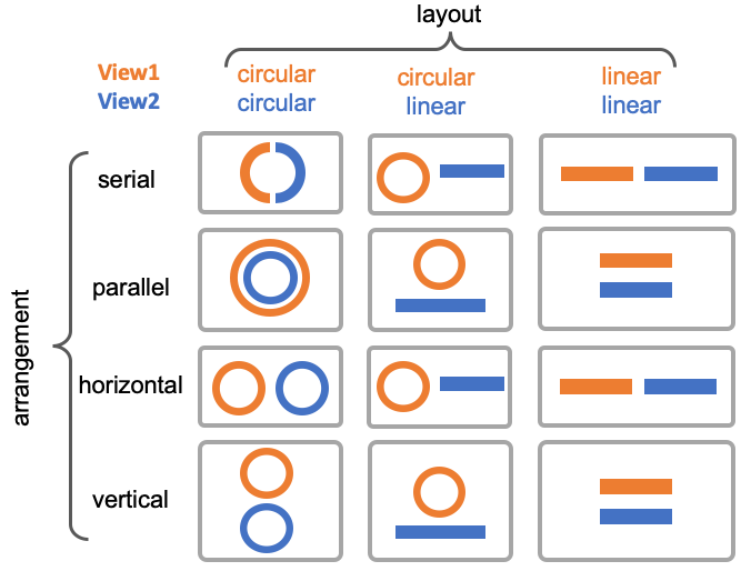 158 |
159 |
160 | ## Inherit Property in Nested Structure
161 |
162 | Both `view` and `track` supports nested structures: One `view` can have several children `views`, and one `track` can have several children `tracks`. Properties can be inherited from upper-level specifications or overwritten locally.
163 |
164 | ```javascript
165 | // nested structures in views
166 | {
167 | "arrangement": "parallel",
168 | "views": [
169 | {/** view **/ },
170 | {/** view **/ },
171 | {
172 | // a view with children views
173 | "arrangement": "parallel",
174 | "views": [...]
175 | }
176 | ]
177 | }
178 | ```
179 |
180 | ```javascript
181 | // nested structures in tracks
182 | {
183 | "alignment":"overlay",
184 | "tracks": [
185 | {
186 | // the parent track
187 | "data": ... , // specify data
188 | "x": ...,
189 | "y": ...,
190 | "color":...,
191 | "alignment": "overlay",
192 | "tracks": [
193 | // the children tracks
194 | // point mark and line mark have the same data, x, y, color encoding
195 | {
196 | "mark": "line",
197 | },
198 | {
199 | "mark": "point",
200 | // specify the size of point mark
201 | "size": {"field": "peak", "type": "quantitative", "range": [0, 6]}
202 | }
203 | ]
204 | }
205 | ]
206 | }
207 | ```
208 |
209 | Use the nested structure if you want to use overlaid tracks inside stacked tracks.
210 |
211 |
212 | Try examples in the online editor:
213 |
214 | [Line chart (line + point)](
158 |
159 |
160 | ## Inherit Property in Nested Structure
161 |
162 | Both `view` and `track` supports nested structures: One `view` can have several children `views`, and one `track` can have several children `tracks`. Properties can be inherited from upper-level specifications or overwritten locally.
163 |
164 | ```javascript
165 | // nested structures in views
166 | {
167 | "arrangement": "parallel",
168 | "views": [
169 | {/** view **/ },
170 | {/** view **/ },
171 | {
172 | // a view with children views
173 | "arrangement": "parallel",
174 | "views": [...]
175 | }
176 | ]
177 | }
178 | ```
179 |
180 | ```javascript
181 | // nested structures in tracks
182 | {
183 | "alignment":"overlay",
184 | "tracks": [
185 | {
186 | // the parent track
187 | "data": ... , // specify data
188 | "x": ...,
189 | "y": ...,
190 | "color":...,
191 | "alignment": "overlay",
192 | "tracks": [
193 | // the children tracks
194 | // point mark and line mark have the same data, x, y, color encoding
195 | {
196 | "mark": "line",
197 | },
198 | {
199 | "mark": "point",
200 | // specify the size of point mark
201 | "size": {"field": "peak", "type": "quantitative", "range": [0, 6]}
202 | }
203 | ]
204 | }
205 | ]
206 | }
207 | ```
208 |
209 | Use the nested structure if you want to use overlaid tracks inside stacked tracks.
210 |
211 |
212 | Try examples in the online editor:
213 |
214 | [Line chart (line + point)]( 40 |
41 | [Try it in the online editor](
40 |
41 | [Try it in the online editor](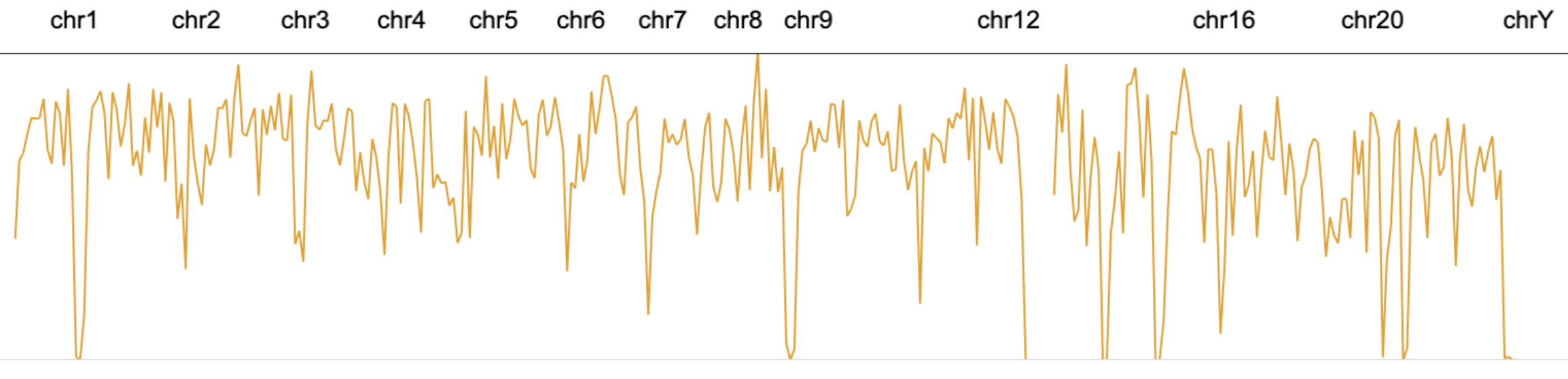 72 |
73 | [Try it in the online editor](
72 |
73 | [Try it in the online editor](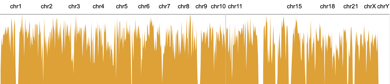 103 |
104 | [Try it in the online editor](
103 |
104 | [Try it in the online editor]( 137 |
138 | [Try it in the online editor](
137 |
138 | [Try it in the online editor]( 170 |
171 | [Try it in the online editor](
170 |
171 | [Try it in the online editor]( 213 |
214 | [Try it in the online editor](
213 |
214 | [Try it in the online editor]( 248 |
249 | [Try it in the online editor](
248 |
249 | [Try it in the online editor](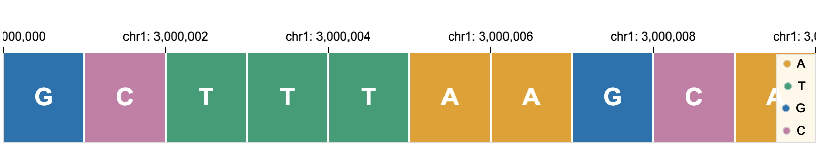 13 |
14 |
13 |
14 | 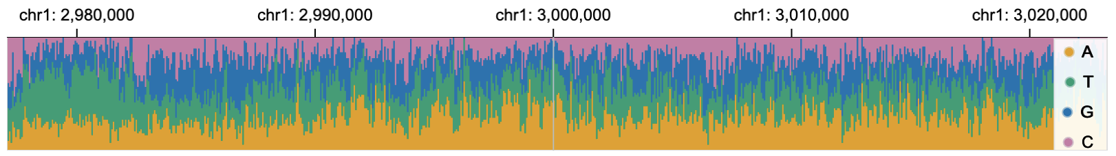 15 |
16 | [Try this example in the online editor](
15 |
16 | [Try this example in the online editor]( 20 |
21 |
20 |
21 |  22 |
23 | **Top**: only `rect` marks are represented; **Bottom:** `text` and `triangle` marks are presented when zooming in to show more details.
24 | [Try this example in the online editor](
22 |
23 | **Top**: only `rect` marks are represented; **Bottom:** `text` and `triangle` marks are presented when zooming in to show more details.
24 | [Try this example in the online editor](> :"greater-than", "gt", "GT",
< : "less-than", "lt", "LT",
≥ : "greater-than-or-equal-to", "gtet", "GTET"),
≤ : "less-than-or-equal-to", "ltet", "LTET" | 39 | | conditionPadding | number | buffer px size of width or height when calculating the visibility, default = 0 | 40 | | transitionPadding | number | buffer px size of width or height for smooth transition, default = 0 | 41 | 42 | The `visibility` of corresponding marks are decided by whether the `measure` of `target` and the `threshold` satisfy the `operation`. 43 | 44 | For example, in the code below, text marks only show when the width (`measure`) of the mark (`target`) is great-than (`operation`) 20 (`threshold`). 45 | 46 | ```javascript 47 | { 48 | // example of semantic zoom: show text marks when zooming in 49 | 50 | "tracks":[{ 51 | "data":..., 52 | "x": ..., 53 | "y": ..., 54 | // overlay overlaps bar marks and text marks for the same data 55 | "alignment": "overlay", 56 | "tracks":[ 57 | //bar marks always show 58 | {"mark": "bar"}, 59 | //text marks only show when the width of mark is great than 20 60 | { 61 | "mark": "text", 62 | "visibility": [{ 63 | "operation": "greater-than", 64 | "measure": "width", 65 | "threshold": "20", 66 | "target": "mark" 67 | }] 68 | } 69 | ] 70 | }] 71 | } 72 | ``` -------------------------------------------------------------------------------- /docs/user-interaction.md: -------------------------------------------------------------------------------- 1 | --- 2 | title: User Interaction 3 | --- 4 | - [Zooming and Panning](#zooming-and-panning) 5 | - [Linking Views](#linking-views) 6 | - [Brushing and Linking](#brushing-and-linking) 7 | 8 | ## Zooming and Panning 9 | 10 | 11 | Each visualization in Gosling supports the Zooming and Panning interaction. 12 | Users can zoom in/out a visualization using the scrolling up/down actions. 13 | Users can pan by clicking on the visualization and then drag it in the desired direction. 14 | 15 | Zooming and panning are controlled through the `static` property, which has a default value of `false`. 16 | When `static = true`, zooming and panning are disabled. 17 | Users can set the `static` property of all tracks at the root level or specify it in a single track definition. 18 | ```javascript 19 | { 20 | "static": true, //disable zoom & pan for all tracks 21 | "tracks": [ 22 | { 23 | "static": false, // enable zoom & pan for this track 24 | ... 25 | }, 26 | { 27 | ... 28 | }, 29 | ... 30 | ] 31 | } 32 | ``` 33 | 34 | ## Linking Views 35 | 36 | 37 | When views/tracks are linked, the zooming and panning performed in one view/track will be automatically applied to the linked views/tracks. 38 | 39 | [Try it in the online editor](
 133 |
134 |
135 |
136 | ## row
137 |
138 | Channel `row` is used with channel `y` to stratify a visualization with categorical values.
139 |
140 | Without specifying `row`:
141 |
142 |
133 |
134 |
135 |
136 | ## row
137 |
138 | Channel `row` is used with channel `y` to stratify a visualization with categorical values.
139 |
140 | Without specifying `row`:
141 |
142 | 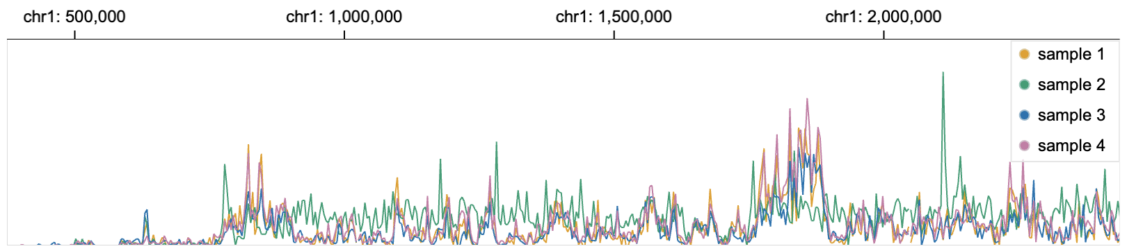 143 |
144 | Line charts are stratified with sample names.
145 |
146 |
143 |
144 | Line charts are stratified with sample names.
145 |
146 | 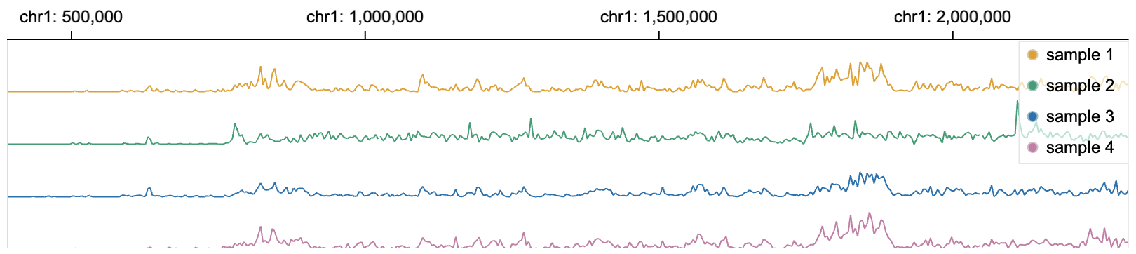 147 |
148 | ```javascript
149 | {
150 | "tracks":[
151 | {
152 | // specify data source
153 | "data": {
154 | "url": "https://resgen.io/api/v1/tileset_info/?d=UvVPeLHuRDiYA3qwFlm7xQ",
155 | "type": "tileset"
156 | },
157 | "metadata": {
158 | "type": "higlass-multivec",
159 | "row": "sample",
160 | "column": "position",
161 | "value": "peak",
162 | "categories": ["sample 1", "sample 2", "sample 3", "sample 4"]
163 | },
164 | // specify the mark type
165 | "mark": "line",
166 | // specify visual channels
167 | "x": {
168 | "field": "position",
169 | "type": "genomic",
170 | "domain": {"chromosome": "1", "interval": [1, 3000500]},
171 | "axis": "top"
172 | },
173 | "y": {"field": "peak", "type": "quantitative"},
174 | "color": {"field": "sample", "type": "nominal", "legend": true},
175 | // visual channel row is bound with the data field: sample
176 | "row": {"field": "sample", "type": "nominal"}
177 | }
178 | ]
179 |
180 | }
181 | ```
182 |
183 | ## size
184 | Channel `size` indicates the size of the visual mark. It determines either the radius of a circle (`mark: point`), the vertical length of a triangle (`mark: triangleRight`, `mark: triangleLeft`, `mark: triangleBottom`), the vertical length of a rectangle (`mark: rect`), the thickness of a line (`mark: line`).
185 |
186 | ## text
187 |
188 | `text` channel is used only in `text` mark to specify what textual information to display.
189 |
190 | ## color
191 | Channel `color` specifies the filling color of the mark. Binding `color` with categorical values in `bar` and `area` marks stack marks that are positioned in the same genomic intervals to better show their cumulative values.
192 |
193 | Apart from the properties shared by all channels, the `color` channel have the following unique properties:
194 |
195 | | unique properties | type | description |
196 | | ----------------- | ------- | -------------------------------- |
197 | | legend | boolean | whether to show the color legend |
198 |
199 | ## stroke
200 | Channel `stroke` defines the outline color of the mark. Gosling supports `stroke` in the following marks: `rect`, `area`, `point`, `bar`, `link`.
201 |
202 | ## strokeWidth
203 | Channel `strokeWidth` defines the outline thickness of the mark shape. Gosling supports `strokeWidth` in the following marks: `rect`, `area`, `point`, `bar`, `link`.
204 |
205 | ## opacity
206 | Channel `opacity` specifies the opacity of the mark shape.
207 |
208 |
209 |
210 |
211 | ## Style
212 |
213 | `style` specifies the visual appearances of a track that are not bound with data fields.
214 |
215 | | style properties | type | description |
216 | | ---------------- | ------------------------------------------------------ | ---------------------------------------- |
217 | | background | string | color of the background |
218 | | dashed | [number, number] |
219 | | linePatterns | { "type": "triangleLeft" \| "triangleRight"; size: number } |
220 | | curve | string | support "top", "bottom", "left", "right" |
221 | | align | string | support "left", "right" |
222 | | dy | number |
223 | | outline | string |
224 | | outlineWidth | number |
225 | | circularLink | boolean |
226 | | textFontSize | number |
227 | | textStroke | string |
228 | | textStrokeWidth | number |
229 | | textFontWeight | string | support "bold", "normal" |
230 |
--------------------------------------------------------------------------------
/images/alignment.png:
--------------------------------------------------------------------------------
https://raw.githubusercontent.com/gosling-lang/gosling-docs/dcbc4f62c2c76d613d691b4d3265a2bb817c1b5d/images/alignment.png
--------------------------------------------------------------------------------
/images/area_example.png:
--------------------------------------------------------------------------------
https://raw.githubusercontent.com/gosling-lang/gosling-docs/dcbc4f62c2c76d613d691b4d3265a2bb817c1b5d/images/area_example.png
--------------------------------------------------------------------------------
/images/bar_example.png:
--------------------------------------------------------------------------------
https://raw.githubusercontent.com/gosling-lang/gosling-docs/dcbc4f62c2c76d613d691b4d3265a2bb817c1b5d/images/bar_example.png
--------------------------------------------------------------------------------
/images/layout_demo.png:
--------------------------------------------------------------------------------
https://raw.githubusercontent.com/gosling-lang/gosling-docs/dcbc4f62c2c76d613d691b4d3265a2bb817c1b5d/images/layout_demo.png
--------------------------------------------------------------------------------
/images/line_example.png:
--------------------------------------------------------------------------------
https://raw.githubusercontent.com/gosling-lang/gosling-docs/dcbc4f62c2c76d613d691b4d3265a2bb817c1b5d/images/line_example.png
--------------------------------------------------------------------------------
/images/linear_circular.png:
--------------------------------------------------------------------------------
https://raw.githubusercontent.com/gosling-lang/gosling-docs/dcbc4f62c2c76d613d691b4d3265a2bb817c1b5d/images/linear_circular.png
--------------------------------------------------------------------------------
/images/link_example.png:
--------------------------------------------------------------------------------
https://raw.githubusercontent.com/gosling-lang/gosling-docs/dcbc4f62c2c76d613d691b4d3265a2bb817c1b5d/images/link_example.png
--------------------------------------------------------------------------------
/images/logo.png:
--------------------------------------------------------------------------------
https://raw.githubusercontent.com/gosling-lang/gosling-docs/dcbc4f62c2c76d613d691b4d3265a2bb817c1b5d/images/logo.png
--------------------------------------------------------------------------------
/images/multi_views.png:
--------------------------------------------------------------------------------
https://raw.githubusercontent.com/gosling-lang/gosling-docs/dcbc4f62c2c76d613d691b4d3265a2bb817c1b5d/images/multi_views.png
--------------------------------------------------------------------------------
/images/point_example.png:
--------------------------------------------------------------------------------
https://raw.githubusercontent.com/gosling-lang/gosling-docs/dcbc4f62c2c76d613d691b4d3265a2bb817c1b5d/images/point_example.png
--------------------------------------------------------------------------------
/images/rect_example.png:
--------------------------------------------------------------------------------
https://raw.githubusercontent.com/gosling-lang/gosling-docs/dcbc4f62c2c76d613d691b4d3265a2bb817c1b5d/images/rect_example.png
--------------------------------------------------------------------------------
/images/semantic_zoom_0.png:
--------------------------------------------------------------------------------
https://raw.githubusercontent.com/gosling-lang/gosling-docs/dcbc4f62c2c76d613d691b4d3265a2bb817c1b5d/images/semantic_zoom_0.png
--------------------------------------------------------------------------------
/images/semantic_zoom_1.png:
--------------------------------------------------------------------------------
https://raw.githubusercontent.com/gosling-lang/gosling-docs/dcbc4f62c2c76d613d691b4d3265a2bb817c1b5d/images/semantic_zoom_1.png
--------------------------------------------------------------------------------
/images/semantic_zoom_2.png:
--------------------------------------------------------------------------------
https://raw.githubusercontent.com/gosling-lang/gosling-docs/dcbc4f62c2c76d613d691b4d3265a2bb817c1b5d/images/semantic_zoom_2.png
--------------------------------------------------------------------------------
/images/semantic_zoom_3.png:
--------------------------------------------------------------------------------
https://raw.githubusercontent.com/gosling-lang/gosling-docs/dcbc4f62c2c76d613d691b4d3265a2bb817c1b5d/images/semantic_zoom_3.png
--------------------------------------------------------------------------------
/images/text_example.png:
--------------------------------------------------------------------------------
https://raw.githubusercontent.com/gosling-lang/gosling-docs/dcbc4f62c2c76d613d691b4d3265a2bb817c1b5d/images/text_example.png
--------------------------------------------------------------------------------
/images/tutorial/tutorial_0.gif:
--------------------------------------------------------------------------------
https://raw.githubusercontent.com/gosling-lang/gosling-docs/dcbc4f62c2c76d613d691b4d3265a2bb817c1b5d/images/tutorial/tutorial_0.gif
--------------------------------------------------------------------------------
/images/tutorial/tutorial_0.png:
--------------------------------------------------------------------------------
https://raw.githubusercontent.com/gosling-lang/gosling-docs/dcbc4f62c2c76d613d691b4d3265a2bb817c1b5d/images/tutorial/tutorial_0.png
--------------------------------------------------------------------------------
/images/tutorial/tutorial_circular.png:
--------------------------------------------------------------------------------
https://raw.githubusercontent.com/gosling-lang/gosling-docs/dcbc4f62c2c76d613d691b4d3265a2bb817c1b5d/images/tutorial/tutorial_circular.png
--------------------------------------------------------------------------------
/images/tutorial/tutorial_dataTransform.png:
--------------------------------------------------------------------------------
https://raw.githubusercontent.com/gosling-lang/gosling-docs/dcbc4f62c2c76d613d691b4d3265a2bb817c1b5d/images/tutorial/tutorial_dataTransform.png
--------------------------------------------------------------------------------
/images/tutorial/tutorial_detail_view1.png:
--------------------------------------------------------------------------------
https://raw.githubusercontent.com/gosling-lang/gosling-docs/dcbc4f62c2c76d613d691b4d3265a2bb817c1b5d/images/tutorial/tutorial_detail_view1.png
--------------------------------------------------------------------------------
/images/tutorial/tutorial_multi_track.png:
--------------------------------------------------------------------------------
https://raw.githubusercontent.com/gosling-lang/gosling-docs/dcbc4f62c2c76d613d691b4d3265a2bb817c1b5d/images/tutorial/tutorial_multi_track.png
--------------------------------------------------------------------------------
/images/tutorial/tutorial_multi_views.gif:
--------------------------------------------------------------------------------
https://raw.githubusercontent.com/gosling-lang/gosling-docs/dcbc4f62c2c76d613d691b4d3265a2bb817c1b5d/images/tutorial/tutorial_multi_views.gif
--------------------------------------------------------------------------------
/images/tutorial/tutorial_overlay.png:
--------------------------------------------------------------------------------
https://raw.githubusercontent.com/gosling-lang/gosling-docs/dcbc4f62c2c76d613d691b4d3265a2bb817c1b5d/images/tutorial/tutorial_overlay.png
--------------------------------------------------------------------------------
/images/tutorial/tutorial_style.png:
--------------------------------------------------------------------------------
https://raw.githubusercontent.com/gosling-lang/gosling-docs/dcbc4f62c2c76d613d691b4d3265a2bb817c1b5d/images/tutorial/tutorial_style.png
--------------------------------------------------------------------------------
/images/tutorial/tutorial_text_label.png:
--------------------------------------------------------------------------------
https://raw.githubusercontent.com/gosling-lang/gosling-docs/dcbc4f62c2c76d613d691b4d3265a2bb817c1b5d/images/tutorial/tutorial_text_label.png
--------------------------------------------------------------------------------
/images/with_row.png:
--------------------------------------------------------------------------------
https://raw.githubusercontent.com/gosling-lang/gosling-docs/dcbc4f62c2c76d613d691b4d3265a2bb817c1b5d/images/with_row.png
--------------------------------------------------------------------------------
/images/without_row.png:
--------------------------------------------------------------------------------
https://raw.githubusercontent.com/gosling-lang/gosling-docs/dcbc4f62c2c76d613d691b4d3265a2bb817c1b5d/images/without_row.png
--------------------------------------------------------------------------------
/images/x_x1_example.png:
--------------------------------------------------------------------------------
https://raw.githubusercontent.com/gosling-lang/gosling-docs/dcbc4f62c2c76d613d691b4d3265a2bb817c1b5d/images/x_x1_example.png
--------------------------------------------------------------------------------
/tutorials/create-multi-track-visualization.md:
--------------------------------------------------------------------------------
1 | ---
2 | title: Multi-track Visualizations
3 | ---
4 | In [Tutorial 1](https://github.com/gosling-lang/gosling-docs/blob/master/tutorials/create-single-track-visualization.md), we introduce how to load data, encode data with marks, transform data, overlay multiple marks and obtain the following visualization.
5 |
147 |
148 | ```javascript
149 | {
150 | "tracks":[
151 | {
152 | // specify data source
153 | "data": {
154 | "url": "https://resgen.io/api/v1/tileset_info/?d=UvVPeLHuRDiYA3qwFlm7xQ",
155 | "type": "tileset"
156 | },
157 | "metadata": {
158 | "type": "higlass-multivec",
159 | "row": "sample",
160 | "column": "position",
161 | "value": "peak",
162 | "categories": ["sample 1", "sample 2", "sample 3", "sample 4"]
163 | },
164 | // specify the mark type
165 | "mark": "line",
166 | // specify visual channels
167 | "x": {
168 | "field": "position",
169 | "type": "genomic",
170 | "domain": {"chromosome": "1", "interval": [1, 3000500]},
171 | "axis": "top"
172 | },
173 | "y": {"field": "peak", "type": "quantitative"},
174 | "color": {"field": "sample", "type": "nominal", "legend": true},
175 | // visual channel row is bound with the data field: sample
176 | "row": {"field": "sample", "type": "nominal"}
177 | }
178 | ]
179 |
180 | }
181 | ```
182 |
183 | ## size
184 | Channel `size` indicates the size of the visual mark. It determines either the radius of a circle (`mark: point`), the vertical length of a triangle (`mark: triangleRight`, `mark: triangleLeft`, `mark: triangleBottom`), the vertical length of a rectangle (`mark: rect`), the thickness of a line (`mark: line`).
185 |
186 | ## text
187 |
188 | `text` channel is used only in `text` mark to specify what textual information to display.
189 |
190 | ## color
191 | Channel `color` specifies the filling color of the mark. Binding `color` with categorical values in `bar` and `area` marks stack marks that are positioned in the same genomic intervals to better show their cumulative values.
192 |
193 | Apart from the properties shared by all channels, the `color` channel have the following unique properties:
194 |
195 | | unique properties | type | description |
196 | | ----------------- | ------- | -------------------------------- |
197 | | legend | boolean | whether to show the color legend |
198 |
199 | ## stroke
200 | Channel `stroke` defines the outline color of the mark. Gosling supports `stroke` in the following marks: `rect`, `area`, `point`, `bar`, `link`.
201 |
202 | ## strokeWidth
203 | Channel `strokeWidth` defines the outline thickness of the mark shape. Gosling supports `strokeWidth` in the following marks: `rect`, `area`, `point`, `bar`, `link`.
204 |
205 | ## opacity
206 | Channel `opacity` specifies the opacity of the mark shape.
207 |
208 |
209 |
210 |
211 | ## Style
212 |
213 | `style` specifies the visual appearances of a track that are not bound with data fields.
214 |
215 | | style properties | type | description |
216 | | ---------------- | ------------------------------------------------------ | ---------------------------------------- |
217 | | background | string | color of the background |
218 | | dashed | [number, number] |
219 | | linePatterns | { "type": "triangleLeft" \| "triangleRight"; size: number } |
220 | | curve | string | support "top", "bottom", "left", "right" |
221 | | align | string | support "left", "right" |
222 | | dy | number |
223 | | outline | string |
224 | | outlineWidth | number |
225 | | circularLink | boolean |
226 | | textFontSize | number |
227 | | textStroke | string |
228 | | textStrokeWidth | number |
229 | | textFontWeight | string | support "bold", "normal" |
230 |
--------------------------------------------------------------------------------
/images/alignment.png:
--------------------------------------------------------------------------------
https://raw.githubusercontent.com/gosling-lang/gosling-docs/dcbc4f62c2c76d613d691b4d3265a2bb817c1b5d/images/alignment.png
--------------------------------------------------------------------------------
/images/area_example.png:
--------------------------------------------------------------------------------
https://raw.githubusercontent.com/gosling-lang/gosling-docs/dcbc4f62c2c76d613d691b4d3265a2bb817c1b5d/images/area_example.png
--------------------------------------------------------------------------------
/images/bar_example.png:
--------------------------------------------------------------------------------
https://raw.githubusercontent.com/gosling-lang/gosling-docs/dcbc4f62c2c76d613d691b4d3265a2bb817c1b5d/images/bar_example.png
--------------------------------------------------------------------------------
/images/layout_demo.png:
--------------------------------------------------------------------------------
https://raw.githubusercontent.com/gosling-lang/gosling-docs/dcbc4f62c2c76d613d691b4d3265a2bb817c1b5d/images/layout_demo.png
--------------------------------------------------------------------------------
/images/line_example.png:
--------------------------------------------------------------------------------
https://raw.githubusercontent.com/gosling-lang/gosling-docs/dcbc4f62c2c76d613d691b4d3265a2bb817c1b5d/images/line_example.png
--------------------------------------------------------------------------------
/images/linear_circular.png:
--------------------------------------------------------------------------------
https://raw.githubusercontent.com/gosling-lang/gosling-docs/dcbc4f62c2c76d613d691b4d3265a2bb817c1b5d/images/linear_circular.png
--------------------------------------------------------------------------------
/images/link_example.png:
--------------------------------------------------------------------------------
https://raw.githubusercontent.com/gosling-lang/gosling-docs/dcbc4f62c2c76d613d691b4d3265a2bb817c1b5d/images/link_example.png
--------------------------------------------------------------------------------
/images/logo.png:
--------------------------------------------------------------------------------
https://raw.githubusercontent.com/gosling-lang/gosling-docs/dcbc4f62c2c76d613d691b4d3265a2bb817c1b5d/images/logo.png
--------------------------------------------------------------------------------
/images/multi_views.png:
--------------------------------------------------------------------------------
https://raw.githubusercontent.com/gosling-lang/gosling-docs/dcbc4f62c2c76d613d691b4d3265a2bb817c1b5d/images/multi_views.png
--------------------------------------------------------------------------------
/images/point_example.png:
--------------------------------------------------------------------------------
https://raw.githubusercontent.com/gosling-lang/gosling-docs/dcbc4f62c2c76d613d691b4d3265a2bb817c1b5d/images/point_example.png
--------------------------------------------------------------------------------
/images/rect_example.png:
--------------------------------------------------------------------------------
https://raw.githubusercontent.com/gosling-lang/gosling-docs/dcbc4f62c2c76d613d691b4d3265a2bb817c1b5d/images/rect_example.png
--------------------------------------------------------------------------------
/images/semantic_zoom_0.png:
--------------------------------------------------------------------------------
https://raw.githubusercontent.com/gosling-lang/gosling-docs/dcbc4f62c2c76d613d691b4d3265a2bb817c1b5d/images/semantic_zoom_0.png
--------------------------------------------------------------------------------
/images/semantic_zoom_1.png:
--------------------------------------------------------------------------------
https://raw.githubusercontent.com/gosling-lang/gosling-docs/dcbc4f62c2c76d613d691b4d3265a2bb817c1b5d/images/semantic_zoom_1.png
--------------------------------------------------------------------------------
/images/semantic_zoom_2.png:
--------------------------------------------------------------------------------
https://raw.githubusercontent.com/gosling-lang/gosling-docs/dcbc4f62c2c76d613d691b4d3265a2bb817c1b5d/images/semantic_zoom_2.png
--------------------------------------------------------------------------------
/images/semantic_zoom_3.png:
--------------------------------------------------------------------------------
https://raw.githubusercontent.com/gosling-lang/gosling-docs/dcbc4f62c2c76d613d691b4d3265a2bb817c1b5d/images/semantic_zoom_3.png
--------------------------------------------------------------------------------
/images/text_example.png:
--------------------------------------------------------------------------------
https://raw.githubusercontent.com/gosling-lang/gosling-docs/dcbc4f62c2c76d613d691b4d3265a2bb817c1b5d/images/text_example.png
--------------------------------------------------------------------------------
/images/tutorial/tutorial_0.gif:
--------------------------------------------------------------------------------
https://raw.githubusercontent.com/gosling-lang/gosling-docs/dcbc4f62c2c76d613d691b4d3265a2bb817c1b5d/images/tutorial/tutorial_0.gif
--------------------------------------------------------------------------------
/images/tutorial/tutorial_0.png:
--------------------------------------------------------------------------------
https://raw.githubusercontent.com/gosling-lang/gosling-docs/dcbc4f62c2c76d613d691b4d3265a2bb817c1b5d/images/tutorial/tutorial_0.png
--------------------------------------------------------------------------------
/images/tutorial/tutorial_circular.png:
--------------------------------------------------------------------------------
https://raw.githubusercontent.com/gosling-lang/gosling-docs/dcbc4f62c2c76d613d691b4d3265a2bb817c1b5d/images/tutorial/tutorial_circular.png
--------------------------------------------------------------------------------
/images/tutorial/tutorial_dataTransform.png:
--------------------------------------------------------------------------------
https://raw.githubusercontent.com/gosling-lang/gosling-docs/dcbc4f62c2c76d613d691b4d3265a2bb817c1b5d/images/tutorial/tutorial_dataTransform.png
--------------------------------------------------------------------------------
/images/tutorial/tutorial_detail_view1.png:
--------------------------------------------------------------------------------
https://raw.githubusercontent.com/gosling-lang/gosling-docs/dcbc4f62c2c76d613d691b4d3265a2bb817c1b5d/images/tutorial/tutorial_detail_view1.png
--------------------------------------------------------------------------------
/images/tutorial/tutorial_multi_track.png:
--------------------------------------------------------------------------------
https://raw.githubusercontent.com/gosling-lang/gosling-docs/dcbc4f62c2c76d613d691b4d3265a2bb817c1b5d/images/tutorial/tutorial_multi_track.png
--------------------------------------------------------------------------------
/images/tutorial/tutorial_multi_views.gif:
--------------------------------------------------------------------------------
https://raw.githubusercontent.com/gosling-lang/gosling-docs/dcbc4f62c2c76d613d691b4d3265a2bb817c1b5d/images/tutorial/tutorial_multi_views.gif
--------------------------------------------------------------------------------
/images/tutorial/tutorial_overlay.png:
--------------------------------------------------------------------------------
https://raw.githubusercontent.com/gosling-lang/gosling-docs/dcbc4f62c2c76d613d691b4d3265a2bb817c1b5d/images/tutorial/tutorial_overlay.png
--------------------------------------------------------------------------------
/images/tutorial/tutorial_style.png:
--------------------------------------------------------------------------------
https://raw.githubusercontent.com/gosling-lang/gosling-docs/dcbc4f62c2c76d613d691b4d3265a2bb817c1b5d/images/tutorial/tutorial_style.png
--------------------------------------------------------------------------------
/images/tutorial/tutorial_text_label.png:
--------------------------------------------------------------------------------
https://raw.githubusercontent.com/gosling-lang/gosling-docs/dcbc4f62c2c76d613d691b4d3265a2bb817c1b5d/images/tutorial/tutorial_text_label.png
--------------------------------------------------------------------------------
/images/with_row.png:
--------------------------------------------------------------------------------
https://raw.githubusercontent.com/gosling-lang/gosling-docs/dcbc4f62c2c76d613d691b4d3265a2bb817c1b5d/images/with_row.png
--------------------------------------------------------------------------------
/images/without_row.png:
--------------------------------------------------------------------------------
https://raw.githubusercontent.com/gosling-lang/gosling-docs/dcbc4f62c2c76d613d691b4d3265a2bb817c1b5d/images/without_row.png
--------------------------------------------------------------------------------
/images/x_x1_example.png:
--------------------------------------------------------------------------------
https://raw.githubusercontent.com/gosling-lang/gosling-docs/dcbc4f62c2c76d613d691b4d3265a2bb817c1b5d/images/x_x1_example.png
--------------------------------------------------------------------------------
/tutorials/create-multi-track-visualization.md:
--------------------------------------------------------------------------------
1 | ---
2 | title: Multi-track Visualizations
3 | ---
4 | In [Tutorial 1](https://github.com/gosling-lang/gosling-docs/blob/master/tutorials/create-single-track-visualization.md), we introduce how to load data, encode data with marks, transform data, overlay multiple marks and obtain the following visualization.
5 |  6 |
6 |
7 |
63 |
64 | This tutorial continues from this example and introduces more advances functions:
65 | - [Semantic Zooming](#semantic-zooming)
66 | - [Multiple Linked Tracks](#multiple-linked-tracks)
67 | - [Circular Layout](#circular-layout)
68 |
69 |
70 | ## Semantic Zooming
71 |
72 | Apart from the default zoom and pan interactions, [semantic zoom](https://github.com/gosling-lang/gosling-docs/blob/master/docs/semantic-zoom.md) is supported in Gosling and allows users to switch between different visualizations of the same data through zooming in/out. When zooming in, the same data will be represented in a different way in which more details are shown.
73 |
74 | Let's say, for this visualization, we want text annotations to show up when zooming in.
75 | We add `text` marks to the `overlay` property and specify when the `text` marks should appear through the `visibility` property.
76 | We may wish the text marks to appear when the distance between chromStart and chromEnd is big enough to place a text mark.
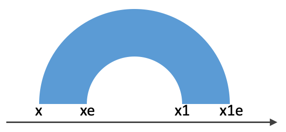
77 | In other words, the text marks appear when the width (`measure`) of the text mark (`target`) is less than (`operation`) than `|xe-x|`.
78 |
79 |
80 | click to expand the code
8 | 9 | ```javascript 10 | { 11 | "tracks":[{ 12 | "width": 700, 13 | "height": 70, 14 | "data": { 15 | "url": "https://raw.githubusercontent.com/sehilyi/gemini-datasets/master/data/UCSC.HG38.Human.CytoBandIdeogram.csv", 16 | "type": "csv", 17 | "chromosomeField": "Chromosome", 18 | "genomicFields": ["chromStart", "chromEnd"] 19 | }, 20 | "x": { 21 | "field": "chromStart", 22 | "type": "genomic", 23 | "domain": {"chromosome": "1"}, 24 | "axis": "top" 25 | }, 26 | "xe": {"field": "chromEnd", "type": "genomic"}, 27 | "alignment": "overlay", 28 | "tracks":[ 29 | { 30 | "mark": "rect", 31 | "dataTransform": [{"type":"filter", "field": "Stain", "oneOf": ["acen"], "not": true}], 32 | "color": { 33 | "field": "Stain", 34 | "type": "nominal", 35 | "domain": ["gpos25", "gpos50", "gpos75", "gpos100"], 36 | "range": ["#D9D9D9","#979797","#636363", "black"] 37 | } 38 | }, 39 | { 40 | "mark": "triangleRight", 41 | "dataTransform": [ 42 | {"type":"filter", "field": "Stain", "oneOf": ["acen"]}, 43 | {"type":"filter", "field": "Name", "include": "q"} 44 | ], 45 | "color": {"value": "#B70101"} 46 | }, 47 | { 48 | "mark": "triangleLeft", 49 | "dataTransform": [ 50 | {"type":"filter", "field": "Stain", "oneOf": ["acen"]}, 51 | {"type":"filter", "field": "Name", "include": "p"} 52 | ], 53 | "color": {"value": "#B70101"} 54 | } 55 | ], 56 | "size": {"value": 20}, 57 | "stroke": {"value": "gray"}, 58 | "strokeWidth": {"value": 0.5} 59 | }] 60 | } 61 | ``` 62 | 81 |
82 | ```diff
83 | {
84 | "tracks": [
85 | {
86 | "width": 700,
87 | "height": 70,
88 | "data": {
89 | "url": "https://raw.githubusercontent.com/sehilyi/gemini-datasets/master/data/UCSC.HG38.Human.CytoBandIdeogram.csv",
90 | "type": "csv",
91 | "chromosomeField": "Chromosome",
92 | "genomicFields": ["chromStart", "chromEnd"]
93 | },
94 | "x": {
95 | "field": "chromStart",
96 | "type": "genomic",
97 | "domain": {"chromosome": "1"},
98 | "axis": "top"
99 | },
100 | "xe": {"field": "chromEnd", "type": "genomic"},
101 | "alignment": "overlay",
102 | "tracks": [
103 | + {
104 | + "mark": "text",
105 | + "dataTransform": [{"type":"filter", "field": "Stain", "oneOf": ["acen"], "not": true}],
106 | + "text": {"field": "Name", "type": "nominal"},
107 | + "color": {
108 | + "field": "Stain",
109 | + "type": "nominal",
110 | + "domain": ["gneg", "gpos25", "gpos50", "gpos75", "gpos100", "gvar"],
111 | + "range": ["black", "black", "black", "black", "white", "black"]
112 | + },
113 | + "visibility": [
114 | + {
115 | + "operation": "less-than",
116 | + "measure": "width",
117 | + "threshold": "|xe-x|",
118 | + "target": "mark"
119 | + }
120 | + ],
121 | + "style": {"textStrokeWidth": 0}
122 | + },
123 | {
124 | "mark": "rect",
125 | "dataTransform": [{"type":"filter", "field": "Stain", "oneOf": ["acen"], "not": true}],
126 | "color": {
127 | "field": "Stain",
128 | "type": "nominal",
129 | "domain": ["gneg", "gpos25", "gpos50", "gpos75", "gpos100", "gvar"],
130 | "range": [
131 | "white",
132 | "#D9D9D9",
133 | "#979797",
134 | "#636363",
135 | "black",
136 | "#A0A0F2"
137 | ]
138 | }
139 | },
140 | {
141 | "mark": "triangleRight",
142 | "dataTransform": [
143 | {"type":"filter", "field": "Stain", "oneOf": ["acen"]},
144 | {"type":"filter", "field": "Name", "include": "q"}
145 | ],
146 | "color": {"value": "#B40101"}
147 | },
148 | {
149 | "mark": "triangleLeft",
150 | "dataTransform": [
151 | {"type":"filter", "field": "Stain", "oneOf": ["acen"]},
152 | {"type":"filter", "field": "Name", "include": "p"}
153 | ],
154 | "color": {"value": "#B40101"}
155 | }
156 | ],
157 | "size": {"value": 20},
158 | "stroke": {"value": "gray"},
159 | "strokeWidth": {"value": 0.5}
160 | }
161 | ]
162 | }
163 | ```
164 |
165 |
166 | ## Multiple Linked Tracks
167 |
168 | We may wish to represent the same data from different aspects using different types of visualization.
169 | To achieve this, we add an area chart (i.e., a new `track`) to the `tracks` property.
170 | Since these tracks share the same `x` coordinate, we wish to link these two tracks: the zooming and panning performed in one track will be automatically applied to the linked track.
171 | In Gosling, `tracks` can be linked by assigning `x` the same `linkingId`.
172 |
173 |
174 |
81 |
82 | ```diff
83 | {
84 | "tracks": [
85 | {
86 | "width": 700,
87 | "height": 70,
88 | "data": {
89 | "url": "https://raw.githubusercontent.com/sehilyi/gemini-datasets/master/data/UCSC.HG38.Human.CytoBandIdeogram.csv",
90 | "type": "csv",
91 | "chromosomeField": "Chromosome",
92 | "genomicFields": ["chromStart", "chromEnd"]
93 | },
94 | "x": {
95 | "field": "chromStart",
96 | "type": "genomic",
97 | "domain": {"chromosome": "1"},
98 | "axis": "top"
99 | },
100 | "xe": {"field": "chromEnd", "type": "genomic"},
101 | "alignment": "overlay",
102 | "tracks": [
103 | + {
104 | + "mark": "text",
105 | + "dataTransform": [{"type":"filter", "field": "Stain", "oneOf": ["acen"], "not": true}],
106 | + "text": {"field": "Name", "type": "nominal"},
107 | + "color": {
108 | + "field": "Stain",
109 | + "type": "nominal",
110 | + "domain": ["gneg", "gpos25", "gpos50", "gpos75", "gpos100", "gvar"],
111 | + "range": ["black", "black", "black", "black", "white", "black"]
112 | + },
113 | + "visibility": [
114 | + {
115 | + "operation": "less-than",
116 | + "measure": "width",
117 | + "threshold": "|xe-x|",
118 | + "target": "mark"
119 | + }
120 | + ],
121 | + "style": {"textStrokeWidth": 0}
122 | + },
123 | {
124 | "mark": "rect",
125 | "dataTransform": [{"type":"filter", "field": "Stain", "oneOf": ["acen"], "not": true}],
126 | "color": {
127 | "field": "Stain",
128 | "type": "nominal",
129 | "domain": ["gneg", "gpos25", "gpos50", "gpos75", "gpos100", "gvar"],
130 | "range": [
131 | "white",
132 | "#D9D9D9",
133 | "#979797",
134 | "#636363",
135 | "black",
136 | "#A0A0F2"
137 | ]
138 | }
139 | },
140 | {
141 | "mark": "triangleRight",
142 | "dataTransform": [
143 | {"type":"filter", "field": "Stain", "oneOf": ["acen"]},
144 | {"type":"filter", "field": "Name", "include": "q"}
145 | ],
146 | "color": {"value": "#B40101"}
147 | },
148 | {
149 | "mark": "triangleLeft",
150 | "dataTransform": [
151 | {"type":"filter", "field": "Stain", "oneOf": ["acen"]},
152 | {"type":"filter", "field": "Name", "include": "p"}
153 | ],
154 | "color": {"value": "#B40101"}
155 | }
156 | ],
157 | "size": {"value": 20},
158 | "stroke": {"value": "gray"},
159 | "strokeWidth": {"value": 0.5}
160 | }
161 | ]
162 | }
163 | ```
164 |
165 |
166 | ## Multiple Linked Tracks
167 |
168 | We may wish to represent the same data from different aspects using different types of visualization.
169 | To achieve this, we add an area chart (i.e., a new `track`) to the `tracks` property.
170 | Since these tracks share the same `x` coordinate, we wish to link these two tracks: the zooming and panning performed in one track will be automatically applied to the linked track.
171 | In Gosling, `tracks` can be linked by assigning `x` the same `linkingId`.
172 |
173 |
174 | 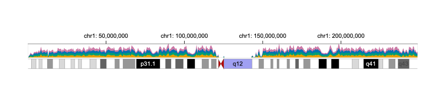 175 |
176 | ```diff
177 | {
178 | + "spacing": 5,
179 | "tracks": [
180 | + {
181 | + "width": 700,
182 | + "height": 40,
183 | + "data": {
184 | + "url": "https://resgen.io/api/v1/tileset_info/?d=UvVPeLHuRDiYA3qwFlm7xQ",
185 | + "type": "multivec",
186 | + "row": "sample",
187 | + "column": "position",
188 | + "value": "peak",
189 | + "categories": ["sample 1", "sample 2", "sample 3", "sample 4"]
190 | + },
191 | + "mark": "area",
192 | + "x": {
193 | + "field": "position",
194 | + "type": "genomic",
195 | + "domain": {"chromosome": "1"},
196 | + "axis": "top",
197 | + "linkingId": "link-1"
198 | + },
199 | + "y": {"field": "peak", "type": "quantitative"},
200 | + "color": {"field": "sample", "type": "nominal"}
201 | + },
202 | {
203 | "width": 700,
204 | - "height": 70,
205 | + "height": 20,
206 | "data": {
207 | "url": "https://raw.githubusercontent.com/sehilyi/gemini-datasets/master/data/UCSC.HG38.Human.CytoBandIdeogram.csv",
208 | "type": "csv",
209 | "chromosomeField": "Chromosome",
210 | "genomicFields": ["chromStart", "chromEnd"]
211 | },
212 | "x": {
213 | "field": "chromStart",
214 | "type": "genomic",
215 | "domain": {"chromosome": "1"},
216 | - "axis": "top"
217 | + "linkingId": "link-1"
218 | },
219 | "xe": {"field": "chromEnd", "type": "genomic"},
220 | "alignment": "overlay",
221 | "tracks": [
222 | {
223 | "mark": "text",
224 | "dataTransform": [{"type":"filter", "field": "Stain", "oneOf": ["acen"], "not": true}],
225 | "text": {"field": "Name", "type": "nominal"},
226 | "color": {
227 | "field": "Stain",
228 | "type": "nominal",
229 | "domain": ["gneg", "gpos25", "gpos50", "gpos75", "gpos100", "gvar"],
230 | "range": ["black", "black", "black", "black", "white", "black"]
231 | },
232 | "visibility": [
233 | {
234 | "operation": "less-than",
235 | "measure": "width",
236 | "threshold": "|xe-x|",
237 | "transitionPadding": 10,
238 | "target": "mark"
239 | }
240 | ],
241 | "style": {"textStrokeWidth": 0}
242 | },
243 | {
244 | "mark": "rect",
245 | "dataTransform": [{"type":"filter", "field": "Stain", "oneOf": ["acen"], "not": true}],
246 | "color": {
247 | "field": "Stain",
248 | "type": "nominal",
249 | "domain": ["gneg", "gpos25", "gpos50", "gpos75", "gpos100", "gvar"],
250 | "range": [
251 | "white",
252 | "#D9D9D9",
253 | "#979797",
254 | "#636363",
255 | "black",
256 | "#A0A0F2"
257 | ]
258 | }
259 | },
260 | {
261 | "mark": "triangleRight",
262 | "dataTransform": [
263 | {"type":"filter", "field": "Stain", "oneOf": ["acen"]},
264 | {"type":"filter", "field": "Name", "include": "q"}
265 | ],
266 | "color": {"value": "#B40101"}
267 | },
268 | {
269 | "mark": "triangleLeft",
270 | "dataTransform": [
271 | {"type":"filter", "field": "Stain", "oneOf": ["acen"]},
272 | {"type":"filter", "field": "Name", "include": "p"}
273 | ],
274 | "color": {"value": "#B40101"}
275 | }
276 | ],
277 | "size": {"value": 20},
278 | "stroke": {"value": "gray"},
279 | "strokeWidth": {"value": 0.5}
280 | }
281 | ]
282 | }
283 | ```
284 |
285 |
286 | ## Circular Layout
287 |
288 | We can easily turn the visualization into a circular layout through the `layout` property.
289 |
290 |
175 |
176 | ```diff
177 | {
178 | + "spacing": 5,
179 | "tracks": [
180 | + {
181 | + "width": 700,
182 | + "height": 40,
183 | + "data": {
184 | + "url": "https://resgen.io/api/v1/tileset_info/?d=UvVPeLHuRDiYA3qwFlm7xQ",
185 | + "type": "multivec",
186 | + "row": "sample",
187 | + "column": "position",
188 | + "value": "peak",
189 | + "categories": ["sample 1", "sample 2", "sample 3", "sample 4"]
190 | + },
191 | + "mark": "area",
192 | + "x": {
193 | + "field": "position",
194 | + "type": "genomic",
195 | + "domain": {"chromosome": "1"},
196 | + "axis": "top",
197 | + "linkingId": "link-1"
198 | + },
199 | + "y": {"field": "peak", "type": "quantitative"},
200 | + "color": {"field": "sample", "type": "nominal"}
201 | + },
202 | {
203 | "width": 700,
204 | - "height": 70,
205 | + "height": 20,
206 | "data": {
207 | "url": "https://raw.githubusercontent.com/sehilyi/gemini-datasets/master/data/UCSC.HG38.Human.CytoBandIdeogram.csv",
208 | "type": "csv",
209 | "chromosomeField": "Chromosome",
210 | "genomicFields": ["chromStart", "chromEnd"]
211 | },
212 | "x": {
213 | "field": "chromStart",
214 | "type": "genomic",
215 | "domain": {"chromosome": "1"},
216 | - "axis": "top"
217 | + "linkingId": "link-1"
218 | },
219 | "xe": {"field": "chromEnd", "type": "genomic"},
220 | "alignment": "overlay",
221 | "tracks": [
222 | {
223 | "mark": "text",
224 | "dataTransform": [{"type":"filter", "field": "Stain", "oneOf": ["acen"], "not": true}],
225 | "text": {"field": "Name", "type": "nominal"},
226 | "color": {
227 | "field": "Stain",
228 | "type": "nominal",
229 | "domain": ["gneg", "gpos25", "gpos50", "gpos75", "gpos100", "gvar"],
230 | "range": ["black", "black", "black", "black", "white", "black"]
231 | },
232 | "visibility": [
233 | {
234 | "operation": "less-than",
235 | "measure": "width",
236 | "threshold": "|xe-x|",
237 | "transitionPadding": 10,
238 | "target": "mark"
239 | }
240 | ],
241 | "style": {"textStrokeWidth": 0}
242 | },
243 | {
244 | "mark": "rect",
245 | "dataTransform": [{"type":"filter", "field": "Stain", "oneOf": ["acen"], "not": true}],
246 | "color": {
247 | "field": "Stain",
248 | "type": "nominal",
249 | "domain": ["gneg", "gpos25", "gpos50", "gpos75", "gpos100", "gvar"],
250 | "range": [
251 | "white",
252 | "#D9D9D9",
253 | "#979797",
254 | "#636363",
255 | "black",
256 | "#A0A0F2"
257 | ]
258 | }
259 | },
260 | {
261 | "mark": "triangleRight",
262 | "dataTransform": [
263 | {"type":"filter", "field": "Stain", "oneOf": ["acen"]},
264 | {"type":"filter", "field": "Name", "include": "q"}
265 | ],
266 | "color": {"value": "#B40101"}
267 | },
268 | {
269 | "mark": "triangleLeft",
270 | "dataTransform": [
271 | {"type":"filter", "field": "Stain", "oneOf": ["acen"]},
272 | {"type":"filter", "field": "Name", "include": "p"}
273 | ],
274 | "color": {"value": "#B40101"}
275 | }
276 | ],
277 | "size": {"value": 20},
278 | "stroke": {"value": "gray"},
279 | "strokeWidth": {"value": 0.5}
280 | }
281 | ]
282 | }
283 | ```
284 |
285 |
286 | ## Circular Layout
287 |
288 | We can easily turn the visualization into a circular layout through the `layout` property.
289 |
290 | 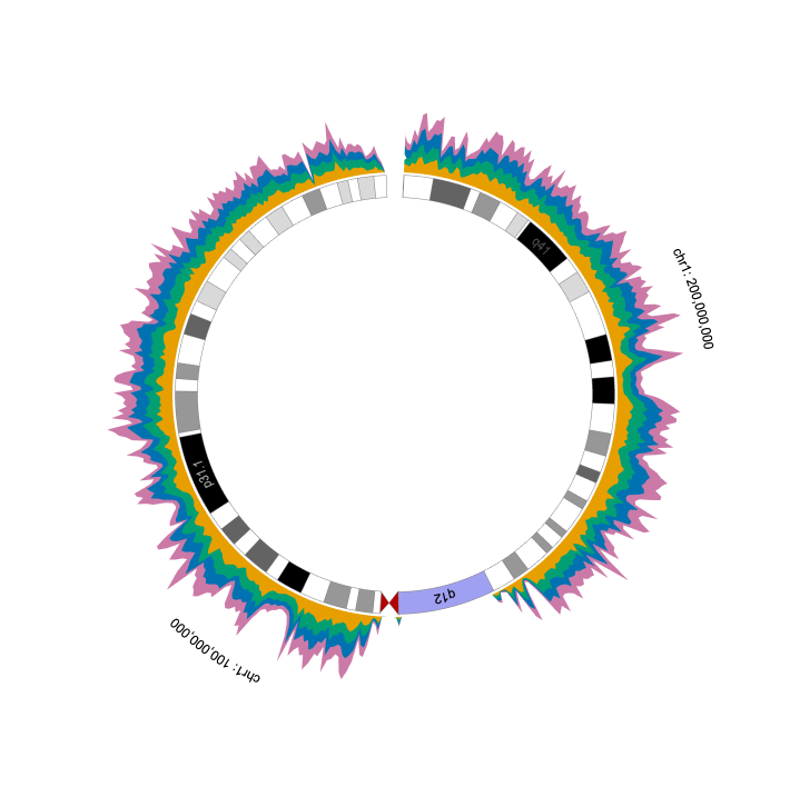 291 |
292 | ```diff
293 | + "layout": "circular",
294 | + "centerRadius": 0.6,
295 | ```
296 |
297 |
291 |
292 | ```diff
293 | + "layout": "circular",
294 | + "centerRadius": 0.6,
295 | ```
296 |
297 |
298 |
409 |
--------------------------------------------------------------------------------
/tutorials/create-multi-view-visualization.md:
--------------------------------------------------------------------------------
1 | ---
2 | title: Multi-view Visualizations
3 | ---
4 | In [Tutorial 2](https://github.com/gosling-lang/gosling-docs/blob/master/tutorials/create-multi-track-visualization.md), we introduce how to create a multi-track visualization, as shown below.
5 |
6 | Click here to expand the complete code
299 | 300 | ```javscript 301 | { 302 | "layout": "circular", 303 | "centerRadius": 0.6, 304 | "spacing": 5, 305 | "tracks": [ 306 | { 307 | "width": 700, 308 | "height": 40, 309 | "data": { 310 | "url": "https://resgen.io/api/v1/tileset_info/?d=UvVPeLHuRDiYA3qwFlm7xQ", 311 | "type": "multivec", 312 | "row": "sample", 313 | "column": "position", 314 | "value": "peak", 315 | "categories": ["sample 1", "sample 2", "sample 3", "sample 4"] 316 | }, 317 | "mark": "area", 318 | "x": { 319 | "field": "position", 320 | "type": "genomic", 321 | "domain": {"chromosome": "1"}, 322 | "axis": "top", 323 | "linkingId": "link-1" 324 | }, 325 | "y": {"field": "peak", "type": "quantitative"}, 326 | "color": {"field": "sample", "type": "nominal"} 327 | }, 328 | { 329 | "width": 700, 330 | "height": 20, 331 | "data": { 332 | "url": "https://raw.githubusercontent.com/sehilyi/gemini-datasets/master/data/UCSC.HG38.Human.CytoBandIdeogram.csv", 333 | "type": "csv", 334 | "chromosomeField": "Chromosome", 335 | "genomicFields": ["chromStart", "chromEnd"] 336 | }, 337 | "x": { 338 | "field": "chromStart", 339 | "type": "genomic", 340 | "domain": {"chromosome": "1"}, 341 | "linkingId": "link-1" 342 | }, 343 | "xe": {"field": "chromEnd", "type": "genomic"}, 344 | "alignment": "overlay", 345 | "tracks": [ 346 | { 347 | "mark": "text", 348 | "dataTransform": [{"type":"filter", "field": "Stain", "oneOf": ["acen"], "not": true}], 349 | "text": {"field": "Name", "type": "nominal"}, 350 | "color": { 351 | "field": "Stain", 352 | "type": "nominal", 353 | "domain": ["gneg", "gpos25", "gpos50", "gpos75", "gpos100", "gvar"], 354 | "range": ["black", "black", "black", "black", "white", "black"] 355 | }, 356 | "visibility": [ 357 | { 358 | "operation": "less-than", 359 | "measure": "width", 360 | "threshold": "|xe-x|", 361 | "transitionPadding": 10, 362 | "target": "mark" 363 | } 364 | ], 365 | "style": {"textStrokeWidth": 0} 366 | }, 367 | { 368 | "mark": "rect", 369 | "dataTransform": [{"type":"filter", "field": "Stain", "oneOf": ["acen"], "not": true}], 370 | "color": { 371 | "field": "Stain", 372 | "type": "nominal", 373 | "domain": ["gneg", "gpos25", "gpos50", "gpos75", "gpos100", "gvar"], 374 | "range": [ 375 | "white", 376 | "#D9D9D9", 377 | "#979797", 378 | "#636363", 379 | "black", 380 | "#A0A0F2" 381 | ] 382 | } 383 | }, 384 | { 385 | "mark": "triangleRight", 386 | "dataTransform": [ 387 | {"type":"filter", "field": "Stain", "oneOf": ["acen"]}, 388 | {"type":"filter", "field": "Name", "include": "q"} 389 | ], 390 | "color": {"value": "#B40101"} 391 | }, 392 | { 393 | "mark": "triangleLeft", 394 | "dataTransform": [ 395 | {"type":"filter", "field": "Stain", "oneOf": ["acen"]}, 396 | {"type":"filter", "field": "Name", "include": "p"} 397 | ], 398 | "color": {"value": "#B40101"} 399 | } 400 | ], 401 | "size": {"value": 20}, 402 | "stroke": {"value": "gray"}, 403 | "strokeWidth": {"value": 0.5} 404 | } 405 | ] 406 | } 407 | ``` 408 |
7 |
8 |
9 |
120 |
121 | In Gosling, we call a visualization with several `tracks` as **a single view**.
122 | Sometimes, we may wish to create a visualization with **multiple views**, e.g., one overview + several detailed views.
123 |
124 | ## create Multiple Views
125 |
126 | Let's say we use the above circular visualization as the overview that visualizes all the chromosomes.
127 | To achieve this, we remove the specified `x.domain` in the overview.
128 | **Overview**
129 | ```diff
130 | - "domain": {"chromosome": "1"},
131 | ```
132 |
133 | We then create two linear detailed views for two different chromosomes, e.g., chromosome 2 and chromosome 5.
134 |
135 |
136 | **Detailed View 1**
137 |
138 | Click here to expand the complete code
10 | 11 | ```javascript 12 | { 13 | "layout": "circular", 14 | "centerRadius": 0.6, 15 | "spacing": 5, 16 | "tracks": [ 17 | { 18 | "width": 700, 19 | "height": 40, 20 | "data": { 21 | "url": "https://resgen.io/api/v1/tileset_info/?d=UvVPeLHuRDiYA3qwFlm7xQ", 22 | "type": "multivec", 23 | "row": "sample", 24 | "column": "position", 25 | "value": "peak", 26 | "categories": ["sample 1", "sample 2", "sample 3", "sample 4"] 27 | }, 28 | "mark": "area", 29 | "x": { 30 | "field": "position", 31 | "type": "genomic", 32 | "domain": {"chromosome": "1"}, 33 | "axis": "top", 34 | "linkingId": "link-1" 35 | }, 36 | "y": {"field": "peak", "type": "quantitative"}, 37 | "color": {"field": "sample", "type": "nominal"} 38 | }, 39 | { 40 | "width": 700, 41 | "height": 20, 42 | "data": { 43 | "url": "https://raw.githubusercontent.com/sehilyi/gemini-datasets/master/data/UCSC.HG38.Human.CytoBandIdeogram.csv", 44 | "type": "csv", 45 | "chromosomeField": "Chromosome", 46 | "genomicFields": ["chromStart", "chromEnd"] 47 | }, 48 | "x": { 49 | "field": "chromStart", 50 | "type": "genomic", 51 | "domain": {"chromosome": "1"}, 52 | "linkingId": "link-1" 53 | }, 54 | "xe": {"field": "chromEnd", "type": "genomic"}, 55 | "alignment": "overlay", 56 | "tracks": [ 57 | { 58 | "mark": "text", 59 | "dataTransform": [{"type":"filter", "field": "Stain", "oneOf": ["acen"], "not": true}], 60 | "text": {"field": "Name", "type": "nominal"}, 61 | "color": { 62 | "field": "Stain", 63 | "type": "nominal", 64 | "domain": ["gneg", "gpos25", "gpos50", "gpos75", "gpos100", "gvar"], 65 | "range": ["black", "black", "black", "black", "white", "black"] 66 | }, 67 | "visibility": [ 68 | { 69 | "operation": "less-than", 70 | "measure": "width", 71 | "threshold": "|xe-x|", 72 | "transitionPadding": 10, 73 | "target": "mark" 74 | } 75 | ], 76 | "style": {"textStrokeWidth": 0} 77 | }, 78 | { 79 | "mark": "rect", 80 | "dataTransform": [{"type":"filter", "field": "Stain", "oneOf": ["acen"], "not": true}], 81 | "color": { 82 | "field": "Stain", 83 | "type": "nominal", 84 | "domain": ["gneg", "gpos25", "gpos50", "gpos75", "gpos100", "gvar"], 85 | "range": [ 86 | "white", 87 | "#D9D9D9", 88 | "#979797", 89 | "#636363", 90 | "black", 91 | "#A0A0F2" 92 | ] 93 | } 94 | }, 95 | { 96 | "mark": "triangleRight", 97 | "dataTransform": [ 98 | {"type":"filter", "field": "Stain", "oneOf": ["acen"]}, 99 | {"type":"filter", "field": "Name", "include": "q"} 100 | ], 101 | "color": {"value": "#B40101"} 102 | }, 103 | { 104 | "mark": "triangleLeft", 105 | "dataTransform": [ 106 | {"type":"filter", "field": "Stain", "oneOf": ["acen"]}, 107 | {"type":"filter", "field": "Name", "include": "p"} 108 | ], 109 | "color": {"value": "#B40101"} 110 | } 111 | ], 112 | "size": {"value": 20}, 113 | "stroke": {"value": "gray"}, 114 | "strokeWidth": {"value": 0.5} 115 | } 116 | ] 117 | } 118 | ``` 119 |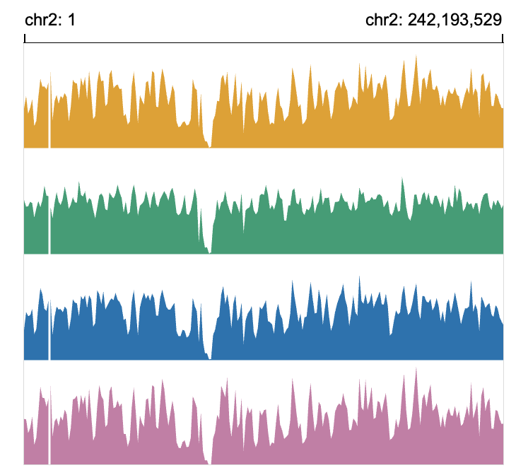 139 |
140 | ```diff
141 | + {
142 | + "layout": "linear",
143 | + "tracks": [{
144 | + "row": {"field": "sample", "type": "nominal"},
145 | + "width": 340,
146 | + "height": 300,
147 | + "data": {
148 | + "url": "https://resgen.io/api/v1/tileset_info/?d=UvVPeLHuRDiYA3qwFlm7xQ",
149 | + "type": "multivec",
150 | + "row": "sample",
151 | + "column": "position",
152 | + "value": "peak",
153 | + "categories": ["sample 1", "sample 2", "sample 3", "sample 4"]
154 | + },
155 | + "mark": "area",
156 | + "x": {
157 | + "field": "position",
158 | + "type": "genomic",
159 | + "domain": {"chromosome": "2"}
160 | + "axis": "top"
161 | + },
162 | + "y": {"field": "peak", "type": "quantitative"},
163 | + "color": {"field": "sample", "type": "nominal"}
164 | + }]
165 | + }
166 | ```
167 |
168 |
169 |
170 | **Detailed View 2** is the same as **Detailed View 1** except the `x.domain`.
171 |
172 | ```diff
173 | - "domain": {"chromosome": "2"}
174 | + "domain": {"chromosome": "5"}
175 | ```
176 |
139 |
140 | ```diff
141 | + {
142 | + "layout": "linear",
143 | + "tracks": [{
144 | + "row": {"field": "sample", "type": "nominal"},
145 | + "width": 340,
146 | + "height": 300,
147 | + "data": {
148 | + "url": "https://resgen.io/api/v1/tileset_info/?d=UvVPeLHuRDiYA3qwFlm7xQ",
149 | + "type": "multivec",
150 | + "row": "sample",
151 | + "column": "position",
152 | + "value": "peak",
153 | + "categories": ["sample 1", "sample 2", "sample 3", "sample 4"]
154 | + },
155 | + "mark": "area",
156 | + "x": {
157 | + "field": "position",
158 | + "type": "genomic",
159 | + "domain": {"chromosome": "2"}
160 | + "axis": "top"
161 | + },
162 | + "y": {"field": "peak", "type": "quantitative"},
163 | + "color": {"field": "sample", "type": "nominal"}
164 | + }]
165 | + }
166 | ```
167 |
168 |
169 |
170 | **Detailed View 2** is the same as **Detailed View 1** except the `x.domain`.
171 |
172 | ```diff
173 | - "domain": {"chromosome": "2"}
174 | + "domain": {"chromosome": "5"}
175 | ```
176 |
177 |
207 |
208 |
209 | ## Arrange Multiple Views
210 | So far, we have created one overview and two detailed views.
211 | In Gosling, multiple views can be arranged using the `arrangement` property.
212 |
213 | ```javascript
214 | {
215 | "arrangement": "parallel"
216 | "views": [
217 | {/** overview **/},
218 | {
219 | "arrangement": "serial",
220 | "spacing": 20,
221 | "views": [
222 | {/** detailed view 1 **/},
223 | {/** detailed view 2 **/}
224 | ]
225 | }
226 | ]
227 | }
228 | ```
229 |
230 | Click to expand the complete code for Detailed View 2
178 | 179 | ```diff 180 | + { 181 | + "layout": "linear", 182 | + "tracks": [{ 183 | + "row": {"field": "sample", "type": "nominal"}, 184 | + "width": 340, 185 | + "height": 300, 186 | + "data": { 187 | + "url": "https://resgen.io/api/v1/tileset_info/?d=UvVPeLHuRDiYA3qwFlm7xQ", 188 | + "type": "multivec", 189 | + "row": "sample", 190 | + "column": "position", 191 | + "value": "peak", 192 | + "categories": ["sample 1", "sample 2", "sample 3", "sample 4"] 193 | + }, 194 | + "mark": "area", 195 | + "x": { 196 | + "field": "position", 197 | + "type": "genomic", 198 | + "domain": {"chromosome": "5"} 199 | + "axis": "top" 200 | + }, 201 | + "y": {"field": "peak", "type": "quantitative"}, 202 | + "color": {"field": "sample", "type": "nominal"} 203 | + }] 204 | + } 205 | ``` 206 |
231 |
551 |
552 |
553 | ## Link Multiple Views
554 | We need to link the overview and the two detailed views.
555 | We overlay two `brush` objects to the overview, and link the two `brush` objects to the two detailed views using `linkingId` (i.e., "detail-1", "detail-2").
556 | To help users visually link the brush objects and the detailed views, we assign the same color to the `brush` of the overview and the `background` of the corresponding detailed view.
557 |
558 | **Overview**
559 | ```diff
560 | + "alignment": "overlay",
561 | + "tracks": [
562 | + {
563 | + "mark": "area"
564 | + },
565 | + {
566 | + "mark": "brush",
567 | + "x": {
568 | + "linkingId": "detail-1"
569 | + },
570 | + "color": {
571 | + "value": "blue"
572 | + }
573 | + },
574 | + {
575 | + "mark": "brush",
576 | + "x": {
577 | + "linkingId": "detail-2"
578 | + },
579 | + "color": {
580 | + "value": "red"
581 | + }
582 | + }
583 | + ]
584 | ```
585 |
586 | **Detailed View 1**
587 | ```diff
588 | + "linkingId": "detail-1",
589 |
590 | + "style": {
591 | + "background": "blue",
592 | + "backgroundOpacity": 0.1
593 | + }
594 | ```
595 |
596 | **Detailed View 2**
597 | ```diff
598 | + "linkingId": "detail-2",
599 |
600 | + "style": {
601 | + "background": "red",
602 | + "backgroundOpacity": 0.1
603 | + }
604 | ```
605 |
606 | Click here to expand the complete code
232 | 233 | ```javascript 234 | { 235 | "arrangement": "vertical", 236 | "views": [ 237 | { 238 | "layout": "circular", 239 | "centerRadius": 0.6, 240 | "spacing": 5, 241 | "tracks": [ 242 | { 243 | "width": 700, 244 | "height": 40, 245 | "data": { 246 | "url": "https://resgen.io/api/v1/tileset_info/?d=UvVPeLHuRDiYA3qwFlm7xQ", 247 | "type": "multivec", 248 | "row": "sample", 249 | "column": "position", 250 | "value": "peak", 251 | "categories": [ 252 | "sample 1", 253 | "sample 2", 254 | "sample 3", 255 | "sample 4" 256 | ] 257 | }, 258 | "mark": "area", 259 | "x": { 260 | "field": "position", 261 | "type": "genomic", 262 | "axis": "top", 263 | "linkingId": "link-1" 264 | }, 265 | "y": { 266 | "field": "peak", 267 | "type": "quantitative" 268 | }, 269 | "color": { 270 | "field": "sample", 271 | "type": "nominal" 272 | }, 273 | "alignment": "overlay", 274 | "tracks": [ 275 | { 276 | "mark": "area" 277 | }, 278 | { 279 | "mark": "brush", 280 | "x": { 281 | "linkingId": "detail-1" 282 | }, 283 | "color": { 284 | "value": "blue" 285 | } 286 | }, 287 | { 288 | "mark": "brush", 289 | "x": { 290 | "linkingId": "detail-2" 291 | }, 292 | "color": { 293 | "value": "red" 294 | } 295 | } 296 | ] 297 | }, 298 | { 299 | "width": 700, 300 | "height": 20, 301 | "data": { 302 | "url": "https://raw.githubusercontent.com/sehilyi/gemini-datasets/master/data/UCSC.HG38.Human.CytoBandIdeogram.csv", 303 | "type": "csv", 304 | "chromosomeField": "Chromosome", 305 | "genomicFields": [ 306 | "chromStart", 307 | "chromEnd" 308 | ] 309 | }, 310 | "x": { 311 | "field": "chromStart", 312 | "type": "genomic" 313 | }, 314 | "xe": { 315 | "field": "chromEnd", 316 | "type": "genomic" 317 | }, 318 | "alignment": "overlay", 319 | "tracks": [ 320 | { 321 | "mark": "text", 322 | "dataTransform": [ 323 | { 324 | "type":"filter", 325 | "field": "Stain", 326 | "oneOf": [ 327 | "acen" 328 | ], 329 | "not": true 330 | } 331 | ], 332 | "text": { 333 | "field": "Name", 334 | "type": "nominal" 335 | }, 336 | "color": { 337 | "field": "Stain", 338 | "type": "nominal", 339 | "domain": [ 340 | "gneg", 341 | "gpos25", 342 | "gpos50", 343 | "gpos75", 344 | "gpos100", 345 | "gvar" 346 | ], 347 | "range": [ 348 | "black", 349 | "black", 350 | "black", 351 | "black", 352 | "white", 353 | "black" 354 | ] 355 | }, 356 | "visibility": [ 357 | { 358 | "operation": "less-than", 359 | "measure": "width", 360 | "threshold": "|xe-x|", 361 | "transitionPadding": 10, 362 | "target": "mark" 363 | } 364 | ], 365 | "style": { 366 | "textStrokeWidth": 0 367 | } 368 | }, 369 | { 370 | "mark": "rect", 371 | "dataTransform": [ 372 | { 373 | "type":"filter", 374 | "field": "Stain", 375 | "oneOf": [ 376 | "acen" 377 | ], 378 | "not": true 379 | } 380 | ], 381 | "color": { 382 | "field": "Stain", 383 | "type": "nominal", 384 | "domain": [ 385 | "gneg", 386 | "gpos25", 387 | "gpos50", 388 | "gpos75", 389 | "gpos100", 390 | "gvar" 391 | ], 392 | "range": [ 393 | "white", 394 | "#D9D9D9", 395 | "#979797", 396 | "#636363", 397 | "black", 398 | "#A0A0F2" 399 | ] 400 | } 401 | }, 402 | { 403 | "mark": "triangleRight", 404 | "dataTransform": [ 405 | { 406 | "type":"filter", 407 | "field": "Stain", 408 | "oneOf": [ 409 | "acen" 410 | ] 411 | }, 412 | { 413 | "type":"filter", 414 | "field": "Name", 415 | "include": "q" 416 | } 417 | ], 418 | "color": { 419 | "value": "#B40101" 420 | } 421 | }, 422 | { 423 | "mark": "triangleLeft", 424 | "dataTransform": [ 425 | { 426 | "type":"filter", 427 | "field": "Stain", 428 | "oneOf": [ 429 | "acen" 430 | ] 431 | }, 432 | { 433 | "type":"filter", 434 | "field": "Name", 435 | "include": "p" 436 | } 437 | ], 438 | "color": { 439 | "value": "#B40101" 440 | } 441 | } 442 | ], 443 | "size": { 444 | "value": 20 445 | }, 446 | "stroke": { 447 | "value": "gray" 448 | }, 449 | "strokeWidth": { 450 | "value": 0.5 451 | } 452 | } 453 | ] 454 | }, 455 | { 456 | "arrangement": "serial", 457 | "spacing": 100, 458 | "views": [ 459 | { 460 | "layout": "linear", 461 | "tracks": [ 462 | { 463 | "row": { 464 | "field": "sample", 465 | "type": "nominal" 466 | }, 467 | "width": 300, 468 | "height": 100, 469 | "data": { 470 | "url": "https://resgen.io/api/v1/tileset_info/?d=UvVPeLHuRDiYA3qwFlm7xQ", 471 | "type": "multivec", 472 | "row": "sample", 473 | "column": "position", 474 | "value": "peak", 475 | "categories": [ 476 | "sample 1", 477 | "sample 2", 478 | "sample 3", 479 | "sample 4" 480 | ] 481 | }, 482 | "mark": "area", 483 | "x": { 484 | "field": "position", 485 | "type": "genomic", 486 | "domain": { 487 | "chromosome": "2" 488 | }, 489 | "axis": "top" 490 | }, 491 | "y": { 492 | "field": "peak", 493 | "type": "quantitative" 494 | }, 495 | "color": { 496 | "field": "sample", 497 | "type": "nominal" 498 | } 499 | } 500 | ] 501 | }, 502 | { 503 | "layout": "linear", 504 | "tracks": [ 505 | { 506 | "row": { 507 | "field": "sample", 508 | "type": "nominal" 509 | }, 510 | "width": 300, 511 | "height": 100, 512 | "data": { 513 | "url": "https://resgen.io/api/v1/tileset_info/?d=UvVPeLHuRDiYA3qwFlm7xQ", 514 | "type": "multivec", 515 | "row": "sample", 516 | "column": "position", 517 | "value": "peak", 518 | "categories": [ 519 | "sample 1", 520 | "sample 2", 521 | "sample 3", 522 | "sample 4" 523 | ] 524 | }, 525 | "mark": "area", 526 | "x": { 527 | "field": "position", 528 | "type": "genomic", 529 | "domain": { 530 | "chromosome": "5" 531 | }, 532 | "axis": "top" 533 | }, 534 | "y": { 535 | "field": "peak", 536 | "type": "quantitative" 537 | }, 538 | "color": { 539 | "field": "sample", 540 | "type": "nominal" 541 | } 542 | } 543 | ] 544 | } 545 | ] 546 | } 547 | ] 548 | } 549 | ``` 550 | 607 |
608 |
607 |
608 |
609 |
--------------------------------------------------------------------------------
/tutorials/create-single-track-visualization.md:
--------------------------------------------------------------------------------
1 | ---
2 | title: Create Single Track Visualization
3 | hide_title: false
4 | slug: /
5 | ---
6 |
7 | This tutorial will guide you step by step in writing the JSON specification to create an interactive cytoband visualization in Gosling.
8 | You will learn about:
9 | - [Loading Data](#loading-data)
10 | - [Encoding Data with Marks](#encoding-data-with-marks)
11 | - [Transforming Data](#transforming-data)
12 | - [Overlaying Multiple Marks](#overlaying-multiple-marks)
13 | - [Coming Up Next](#coming-up-next)
14 |
15 | You are encouraged to follow the tutorial and create visualizations in the [online editor][onlineEditorURL].
16 |
17 | ## Loading Data
18 |
19 | In this tutorial, we use a CSV data that contains UCSC hg38 cytoband information ([the complete data file][csvDataURL]).
20 |
21 |
22 |
23 | |Chromosome|chromStart|chromEnd|Name|Stain|
24 | |---|---|---|---|--|
25 | |chr1|0|2300000|p36.33|gneg|
26 | |chr1|2300000|5300000|p36.32|gpos25|
27 | |chr1|5300000|770000|p36.31|gneg|
28 | |...|
29 |
30 |
31 | To start with, we load this data through URL to a visualization (i.e., a `track`).
32 | The `track.data` property specifies how to fetch and process the data.
33 | ```javascript
34 |
35 | {
36 | "tracks":[{
37 | // Load a csv data file through URL
38 | "data": {
39 | "url": "https://raw.githubusercontent.com/sehilyi/gemini-datasets/master/data/UCSC.HG38.Human.CytoBandIdeogram.csv",
40 | "chromosomeField": "Chromosome",
41 | "type": "csv",
42 | "genomicFields": ["chromStart", "chromEnd"]
43 | }
44 | }]
45 | }
46 | ```
47 |
48 | ## Encoding Data with Marks
49 | After loading the data, we now specify how to visualize the data.
50 | This process is achieved by binding the values of data fields to the visual channels (e.g., color, size) of a graphic element (i.e., `mark`).
51 |
52 | Let's say we use a `rect` mark for the loaded csv data.
53 | Each `rect` represents a chromosome.
54 | The x-coordinate of the mark's start (`x`) and end (`xe`) position indicate the chromStart and the chromeEnd, respectively.
55 | The `color` indicates the stain value.
56 |
57 | For each visual channel, Gosling creates a mapping from the values of the data field (e.g., [gnes, gpos25, gpos50, ...]) to the values of the visual channel (e.g., color). We call the values of data field **domain** and the values of the visual channel **range**.
58 | This mapping is specified by the following properties:
59 |
60 | | visual channel properties | type | description |
61 | | ------------------------- | --------------------------- | ---------------------------------------------------------------------------------- |
62 | | field | string | specify name of the data field |
63 | | type | string | specify type of the data field. support `"genomic"`, `"nominal"`, `"quantitative"` |
64 | | domain | [number, number]\| string[] | specify values of the data field |
65 | | range | [number, number]\| string[] | specify values of the visual channel |
66 |
67 |
68 | ```javascript
69 | {
70 | "tracks":[{
71 | // specify the size of the visualization
72 | "width": 700,
73 | "height": 70,
74 | // Load a csv data file through URL
75 | "data": {
76 | "url": "https://raw.githubusercontent.com/sehilyi/gemini-datasets/master/data/UCSC.HG38.Human.CytoBandIdeogram.csv",
77 | "chromosomeField": "Chromosome",
78 | "type": "csv",
79 | "genomicFields": ["chromStart", "chromEnd"]
80 | },
81 | // specify the mark type
82 | "mark": "rect",
83 | // encoding data with visual channels
84 | "x": {
85 | "field": "chromStart",
86 | "type": "genomic",
87 | "domain": {"chromosome": "1"},
88 | "axis": "top"
89 | },
90 | "xe": {"field": "chromEnd", "type": "genomic"},
91 | "color": {
92 | "field": "Stain",
93 | "type": "nominal",
94 | "domain": ["gneg", "gpos25", "gpos50", "gpos75", "gpos100", "gvar"],
95 | "range": ["white","#D9D9D9","#979797","#636363", "black","#A0A0F2"]
96 | },
97 | // customize the style of the visual marks.
98 | // default values will be used if not specifyed.
99 | "size": {"value": 20},
100 | "stroke": {"value": "gray"},
101 | "strokeWidth": {"value": 0.5}
102 | }]
103 | }
104 | ```
105 |
106 | Click here to expand the complete code
610 | 611 | ```javascript 612 | { 613 | "arrangement": "vertical", 614 | "views": [ 615 | { 616 | "layout": "circular", 617 | "centerRadius": 0.6, 618 | "spacing": 5, 619 | "tracks": [ 620 | { 621 | "width": 700, 622 | "height": 40, 623 | "data": { 624 | "url": "https://resgen.io/api/v1/tileset_info/?d=UvVPeLHuRDiYA3qwFlm7xQ", 625 | "type": "multivec", 626 | "row": "sample", 627 | "column": "position", 628 | "value": "peak", 629 | "categories": ["sample 1", "sample 2", "sample 3", "sample 4"] 630 | }, 631 | "mark": "area", 632 | "x": { 633 | "field": "position", 634 | "type": "genomic", 635 | "axis": "top", 636 | "linkingId": "link-1" 637 | }, 638 | "y": { "field": "peak", "type": "quantitative" }, 639 | "color": { "field": "sample", "type": "nominal" }, 640 | "alignment": "overlay", 641 | "tracks": [ 642 | { "mark": "area" }, 643 | { 644 | "mark": "brush", 645 | "x": { "linkingId": "detail-1" }, 646 | "color": { "value": "blue" } 647 | }, 648 | { 649 | "mark": "brush", 650 | "x": { "linkingId": "detail-2" }, 651 | "color": { "value": "red" } 652 | } 653 | ] 654 | }, 655 | { 656 | "width": 700, 657 | "height": 20, 658 | "data": { 659 | "url": "https://raw.githubusercontent.com/sehilyi/gemini-datasets/master/data/UCSC.HG38.Human.CytoBandIdeogram.csv", 660 | "type": "csv", 661 | "chromosomeField": "Chromosome", 662 | "genomicFields": ["chromStart", "chromEnd"] 663 | }, 664 | "x": { 665 | "field": "chromStart", 666 | "type": "genomic", 667 | "linkingId": "link-1" 668 | }, 669 | "xe": { "field": "chromEnd", "type": "genomic" }, 670 | "alignment": "overlay", 671 | "tracks": [ 672 | { 673 | "mark": "text", 674 | "dataTransform": [{"type":"filter", "field": "Stain", "oneOf": ["acen"], "not": true }], 675 | "text": { "field": "Name", "type": "nominal" }, 676 | "color": { 677 | "field": "Stain", 678 | "type": "nominal", 679 | "domain": ["gneg", "gpos25", "gpos50", "gpos75", "gpos100", "gvar"], 680 | "range": ["black", "black", "black", "black", "white", "black"] 681 | }, 682 | "visibility": [ 683 | { 684 | "operation": "less-than", 685 | "measure": "width", 686 | "threshold": "|xe-x|", 687 | "transitionPadding": 10, 688 | "target": "mark" 689 | } 690 | ], 691 | "style": { "textStrokeWidth": 0 } 692 | }, 693 | { 694 | "mark": "rect", 695 | "dataTransform": [{"type":"filter", "field": "Stain", "oneOf": ["acen"], "not": true }], 696 | "color": { 697 | "field": "Stain", 698 | "type": "nominal", 699 | "domain": ["gneg", "gpos25", "gpos50", "gpos75", "gpos100", "gvar"], 700 | "range": [ 701 | "white", 702 | "#D9D9D9", 703 | "#979797", 704 | "#636363", 705 | "black", 706 | "#A0A0F2" 707 | ] 708 | } 709 | }, 710 | { 711 | "mark": "triangleRight", 712 | "dataTransform": [ 713 | {"type":"filter", "field": "Stain", "oneOf": ["acen"] }, 714 | {"type":"filter", "field": "Name", "include": "q" } 715 | ], 716 | "color": { "value": "#B40101" } 717 | }, 718 | { 719 | "mark": "triangleLeft", 720 | "dataTransform": [ 721 | {"type":"filter", "field": "Stain", "oneOf": ["acen"] }, 722 | {"type":"filter", "field": "Name", "include": "p" } 723 | ], 724 | "color": { "value": "#B40101" } 725 | } 726 | ], 727 | "size": { "value": 20 }, 728 | "stroke": { "value": "gray" }, 729 | "strokeWidth": { "value": 0.5 } 730 | } 731 | ] 732 | }, 733 | { 734 | "arrangement": "serial", 735 | "spacing": 20, 736 | "views": [ 737 | { 738 | "layout": "linear", 739 | "tracks": [ 740 | { 741 | "row": { "field": "sample", "type": "nominal" }, 742 | "width": 340, 743 | "height": 300, 744 | "data": { 745 | "url": "https://resgen.io/api/v1/tileset_info/?d=UvVPeLHuRDiYA3qwFlm7xQ", 746 | "type": "multivec", 747 | "row": "sample", 748 | "column": "position", 749 | "value": "peak", 750 | "categories": ["sample 1", "sample 2", "sample 3", "sample 4"] 751 | }, 752 | "mark": "area", 753 | "x": { 754 | "field": "position", 755 | "type": "genomic", 756 | "domain": { "chromosome": "2" }, 757 | "linkingId": "detail-1", 758 | "axis": "top" 759 | }, 760 | "y": { "field": "peak", "type": "quantitative" }, 761 | "color": { "field": "sample", "type": "nominal" }, 762 | "style": { "background": "blue", "backgroundOpacity": 0.1 } 763 | } 764 | ] 765 | }, 766 | { 767 | "layout": "linear", 768 | "tracks": [{ 769 | "row": { "field": "sample", "type": "nominal" }, 770 | "width": 340, 771 | "height": 300, 772 | "data": { 773 | "url": "https://resgen.io/api/v1/tileset_info/?d=UvVPeLHuRDiYA3qwFlm7xQ", 774 | "type": "multivec", 775 | "row": "sample", 776 | "column": "position", 777 | "value": "peak", 778 | "categories": ["sample 1", "sample 2", "sample 3", "sample 4"] 779 | }, 780 | "mark": "area", 781 | "x": { 782 | "field": "position", 783 | "type": "genomic", 784 | "domain": { "chromosome": "5" }, 785 | "linkingId": "detail-2", 786 | "axis": "top" 787 | }, 788 | "y": { "field": "peak", "type": "quantitative" }, 789 | "color": { "field": "sample", "type": "nominal" }, 790 | "style": { "background": "red", "backgroundOpacity": 0.1 } 791 | }] 792 | } 793 | ] 794 | } 795 | ] 796 | } 797 | ``` 798 | 107 |
108 | **:tada: :tada: :tada: :tada: :tada: :tada: :tada: :tada:**
109 | **You have just created a scalable and interactive visualization in Gosling!**
110 | You can interact with the visualization you just created in the online editor through zoom and pan.
111 | Or, you can keep reading the tutorial and make your visualizations even more fancy.
112 |
113 | ## Transforming Data
114 | Gossling supports filtering out uninterested data through the `dataTransform` property.
115 | For example, we can add a filter to only visualize chromosomes whose stain result is one of "gpos25", "gpos50", "gpos75", or "gpos100".
116 |
117 | ```diff
118 | {
119 | "tracks":[{
120 | "width": 700,
121 | "height": 70,
122 | "data": {
123 | "url": "https://raw.githubusercontent.com/sehilyi/gemini-datasets/master/data/UCSC.HG38.Human.CytoBandIdeogram.csv",
124 | "chromosomeField": "Chromosome",
125 | "type": "csv",
126 | "genomicFields": ["chromStart", "chromEnd"]
127 | },
128 | + "dataTransform": [{"type":"filter", "field": "Stain", "oneOf": ["gpos25", "gpos50", "gpos75", "gpos100"]}],
129 | "mark": "rect",
130 | "x": {
131 | "field": "chromStart",
132 | "type": "genomic",
133 | "domain": {"chromosome": "1"},
134 | "axis": "top"
135 | },
136 | "xe": {"field": "chromEnd", "type": "genomic"},
137 | "color": {
138 | "field": "Stain",
139 | "type": "nominal",
140 | "domain": ["gneg", "gpos25", "gpos50", "gpos75", "gpos100", "gvar"],
141 | "range": ["white","#D9D9D9","#979797","#636363", "black","#A0A0F2"]
142 | },
143 | "size": {"value": 20},
144 | "stroke": {"value": "gray"},
145 | "strokeWidth": {"value": 0.5}
146 | }]
147 | }
148 | ```
149 |
150 |
107 |
108 | **:tada: :tada: :tada: :tada: :tada: :tada: :tada: :tada:**
109 | **You have just created a scalable and interactive visualization in Gosling!**
110 | You can interact with the visualization you just created in the online editor through zoom and pan.
111 | Or, you can keep reading the tutorial and make your visualizations even more fancy.
112 |
113 | ## Transforming Data
114 | Gossling supports filtering out uninterested data through the `dataTransform` property.
115 | For example, we can add a filter to only visualize chromosomes whose stain result is one of "gpos25", "gpos50", "gpos75", or "gpos100".
116 |
117 | ```diff
118 | {
119 | "tracks":[{
120 | "width": 700,
121 | "height": 70,
122 | "data": {
123 | "url": "https://raw.githubusercontent.com/sehilyi/gemini-datasets/master/data/UCSC.HG38.Human.CytoBandIdeogram.csv",
124 | "chromosomeField": "Chromosome",
125 | "type": "csv",
126 | "genomicFields": ["chromStart", "chromEnd"]
127 | },
128 | + "dataTransform": [{"type":"filter", "field": "Stain", "oneOf": ["gpos25", "gpos50", "gpos75", "gpos100"]}],
129 | "mark": "rect",
130 | "x": {
131 | "field": "chromStart",
132 | "type": "genomic",
133 | "domain": {"chromosome": "1"},
134 | "axis": "top"
135 | },
136 | "xe": {"field": "chromEnd", "type": "genomic"},
137 | "color": {
138 | "field": "Stain",
139 | "type": "nominal",
140 | "domain": ["gneg", "gpos25", "gpos50", "gpos75", "gpos100", "gvar"],
141 | "range": ["white","#D9D9D9","#979797","#636363", "black","#A0A0F2"]
142 | },
143 | "size": {"value": 20},
144 | "stroke": {"value": "gray"},
145 | "strokeWidth": {"value": 0.5}
146 | }]
147 | }
148 | ```
149 |
150 | 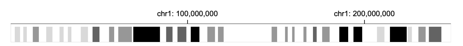 151 |
152 | gvar (purple rect) and gneg (white rect) are not shown in the updated visualization.
153 |
154 |
155 |
156 |
157 |
158 | ## Overlaying Multiple Marks
159 | Multiple `mark` shapes can be put on the top of one another by setting `alignment` as `"overlay"`.
160 | In the code below, a chromosome is visualized as a `triangleRight` mark if its stain result is `acen` and its name includes `q`; a chromosome is visualized as a `triangleLeft` mark if its stain result is `acen` and its name includes `p`. The `rect` mark, the `triangleRight` mark, and the `triangleLeft` mark are overlaid on the same genomic coordinate by setting `alignment` as `"overlay"`.
161 |
162 | ```diff
163 | {
164 | "tracks":[{
165 | "width": 700,
166 | "height": 70,
167 | "data": {
168 | "url": "https://raw.githubusercontent.com/sehilyi/gemini-datasets/master/data/UCSC.HG38.Human.CytoBandIdeogram.csv",
169 | "type": "csv",
170 | "chromosomeField": "Chromosome",
171 | "genomicFields": ["chromStart", "chromEnd"]
172 | },
173 | - "dataTransform": [{"type":"filter", "field": "Stain", "oneOf": ["gpos25", "gpos50", "gpos75", "gpos100"]}],
174 | - "mark": "rect",
175 | "x": {
176 | "field": "chromStart",
177 | "type": "genomic",
178 | "domain": {"chromosome": "1"},
179 | "axis": "top"
180 | },
181 | "xe": {"field": "chromEnd", "type": "genomic"},
182 | - "color": {
183 | - "field": "Stain",
184 | - "type": "nominal",
185 | - "domain": ["gpos25", "gpos50", "gpos75", "gpos100"],
186 | - "range": ["#D9D9D9","#979797","#636363", "black"]
187 | - },
188 | + "alignment": "overlay",
189 | + "tracks":[
190 | + {
191 | + "mark": "rect",
192 | + "dataTransform": [{"type":"filter", "field": "Stain", "oneOf": ["acen"], "not": true}],
193 | + "color": {
194 | + "field": "Stain",
195 | + "type": "nominal",
196 | + "domain": ["gneg", "gpos25", "gpos50", "gpos75", "gpos100", "gvar"],
197 | + "range": ["white","#D9D9D9","#979797","#636363", "black","#A0A0F2"]
198 | + }
199 | + },
200 | + {
201 | + "mark": "triangleRight",
202 | + "dataTransform": [
203 | + {"type":"filter", "field": "Stain", "oneOf": ["acen"]},
204 | + {"type":"filter", "field": "Name", "include": "q"}
205 | + ],
206 | + "color": {"value": "#B70101"}
207 | + },
208 | + {
209 | + "mark": "triangleLeft",
210 | + "dataTransform": [
211 | + {"type":"filter", "field": "Stain", "oneOf": ["acen"]},
212 | + {"type":"filter", "field": "Name", "include": "p"}
213 | + ],
214 | + "color": {"value": "#B70101"}
215 | + }
216 | + ],
217 | "size": {"value": 20},
218 | "stroke": {"value": "gray"},
219 | "strokeWidth": {"value": 0.5}
220 | }]
221 | }
222 | ```
223 |
224 |
225 |
226 |
227 | ## Coming Up Next
228 | [Tutorial 2](https://github.com/gosling-lang/gosling-docs/blob/master/tutorials/create-multi-track-visualization.md): how to use semantic zooming, multiple tracks, and circular layout in Gosling.
229 |
230 | [Tutorial 3](https://github.com/gosling-lang/gosling-docs/blob/master/tutorials/create-multi-view-visualization.md): how to arrange and link multiple views in Gosling.
231 |
232 | You can find more examples [here][exampleURL].
233 |
234 | [onlineEditorURL]: http://gosling.js.org
235 | [exampleURL]: http://gosling.js.org
236 | [csvDataURL]: https://raw.githubusercontent.com/sehilyi/gemini-datasets/master/data/UCSC.HG38.Human.CytoBandIdeogram.csv
237 |
--------------------------------------------------------------------------------
151 |
152 | gvar (purple rect) and gneg (white rect) are not shown in the updated visualization.
153 |
154 |
155 |
156 |
157 |
158 | ## Overlaying Multiple Marks
159 | Multiple `mark` shapes can be put on the top of one another by setting `alignment` as `"overlay"`.
160 | In the code below, a chromosome is visualized as a `triangleRight` mark if its stain result is `acen` and its name includes `q`; a chromosome is visualized as a `triangleLeft` mark if its stain result is `acen` and its name includes `p`. The `rect` mark, the `triangleRight` mark, and the `triangleLeft` mark are overlaid on the same genomic coordinate by setting `alignment` as `"overlay"`.
161 |
162 | ```diff
163 | {
164 | "tracks":[{
165 | "width": 700,
166 | "height": 70,
167 | "data": {
168 | "url": "https://raw.githubusercontent.com/sehilyi/gemini-datasets/master/data/UCSC.HG38.Human.CytoBandIdeogram.csv",
169 | "type": "csv",
170 | "chromosomeField": "Chromosome",
171 | "genomicFields": ["chromStart", "chromEnd"]
172 | },
173 | - "dataTransform": [{"type":"filter", "field": "Stain", "oneOf": ["gpos25", "gpos50", "gpos75", "gpos100"]}],
174 | - "mark": "rect",
175 | "x": {
176 | "field": "chromStart",
177 | "type": "genomic",
178 | "domain": {"chromosome": "1"},
179 | "axis": "top"
180 | },
181 | "xe": {"field": "chromEnd", "type": "genomic"},
182 | - "color": {
183 | - "field": "Stain",
184 | - "type": "nominal",
185 | - "domain": ["gpos25", "gpos50", "gpos75", "gpos100"],
186 | - "range": ["#D9D9D9","#979797","#636363", "black"]
187 | - },
188 | + "alignment": "overlay",
189 | + "tracks":[
190 | + {
191 | + "mark": "rect",
192 | + "dataTransform": [{"type":"filter", "field": "Stain", "oneOf": ["acen"], "not": true}],
193 | + "color": {
194 | + "field": "Stain",
195 | + "type": "nominal",
196 | + "domain": ["gneg", "gpos25", "gpos50", "gpos75", "gpos100", "gvar"],
197 | + "range": ["white","#D9D9D9","#979797","#636363", "black","#A0A0F2"]
198 | + }
199 | + },
200 | + {
201 | + "mark": "triangleRight",
202 | + "dataTransform": [
203 | + {"type":"filter", "field": "Stain", "oneOf": ["acen"]},
204 | + {"type":"filter", "field": "Name", "include": "q"}
205 | + ],
206 | + "color": {"value": "#B70101"}
207 | + },
208 | + {
209 | + "mark": "triangleLeft",
210 | + "dataTransform": [
211 | + {"type":"filter", "field": "Stain", "oneOf": ["acen"]},
212 | + {"type":"filter", "field": "Name", "include": "p"}
213 | + ],
214 | + "color": {"value": "#B70101"}
215 | + }
216 | + ],
217 | "size": {"value": 20},
218 | "stroke": {"value": "gray"},
219 | "strokeWidth": {"value": 0.5}
220 | }]
221 | }
222 | ```
223 |
224 |
225 |
226 |
227 | ## Coming Up Next
228 | [Tutorial 2](https://github.com/gosling-lang/gosling-docs/blob/master/tutorials/create-multi-track-visualization.md): how to use semantic zooming, multiple tracks, and circular layout in Gosling.
229 |
230 | [Tutorial 3](https://github.com/gosling-lang/gosling-docs/blob/master/tutorials/create-multi-view-visualization.md): how to arrange and link multiple views in Gosling.
231 |
232 | You can find more examples [here][exampleURL].
233 |
234 | [onlineEditorURL]: http://gosling.js.org
235 | [exampleURL]: http://gosling.js.org
236 | [csvDataURL]: https://raw.githubusercontent.com/sehilyi/gemini-datasets/master/data/UCSC.HG38.Human.CytoBandIdeogram.csv
237 |
--------------------------------------------------------------------------------