├── .gitignore
├── LICENSE
├── MANIFEST.in
├── README.md
├── examples
├── Black Scholes and Option Greeks.ipynb
├── README.ipynb
├── Visualizing Greeks.ipynb
└── visualizing-options-in-python-using-opstrat.ipynb
├── opstrat
├── __init__.py
├── basic_multi.py
├── basic_single.py
├── blackscholes.py
├── helpers.py
└── yf.py
├── readme_files
├── fig1.png
├── fig2.png
├── fig3.png
├── fig4.png
├── fig5.png
├── fig6.png
└── simple_option.jpeg
├── requirements.txt
└── setup.py
/.gitignore:
--------------------------------------------------------------------------------
1 | # Byte-compiled / optimized / DLL files
2 | __pycache__/
3 | *.py[cod]
4 | *$py.class
5 |
6 | # C extensions
7 | *.so
8 |
9 | #VS Code
10 | .vscode/
11 |
12 | # Distribution / packaging
13 | .Python
14 | env/
15 | build/
16 | develop-eggs/
17 | dist/
18 | downloads/
19 | eggs/
20 | .eggs/
21 | lib/
22 | lib64/
23 | parts/
24 | sdist/
25 | var/
26 | *.egg-info/
27 | .installed.cfg
28 | *.egg
29 |
30 | #My Files
31 | myfiles/
32 |
33 | # PyInstaller
34 | # Usually these files are written by a python script from a template
35 | # before PyInstaller builds the exe, so as to inject date/other infos into it.
36 | *.manifest
37 | *.spec
38 |
39 | # Installer logs
40 | pip-log.txt
41 | pip-delete-this-directory.txt
42 |
43 | # Unit test / coverage reports
44 | htmlcov/
45 | .tox/
46 | .coverage
47 | .coverage.*
48 | .cache
49 | nosetests.xml
50 | coverage.xml
51 | *,cover
52 | .hypothesis/
53 |
54 | # Translations
55 | *.mo
56 | *.pot
57 |
58 | # IPython Notebook
59 | .ipynb_checkpoints
60 |
61 | # pyenv
62 | .python-version
63 |
64 | # celery beat schedule file
65 | celerybeat-schedule
66 |
67 | # dotenv
68 | .env
69 |
70 | # virtualenv
71 | venv/
72 | ENV/
73 |
74 | # Spyder project settings
75 | .spyderproject
76 |
77 | # Rope project settings
78 | .ropeproject
79 | *.npy
80 | *.pkl
--------------------------------------------------------------------------------
/LICENSE:
--------------------------------------------------------------------------------
1 | MIT License
2 |
3 | Copyright (c) 2021 abhijith-git
4 |
5 | Permission is hereby granted, free of charge, to any person obtaining a copy
6 | of this software and associated documentation files (the "Software"), to deal
7 | in the Software without restriction, including without limitation the rights
8 | to use, copy, modify, merge, publish, distribute, sublicense, and/or sell
9 | copies of the Software, and to permit persons to whom the Software is
10 | furnished to do so, subject to the following conditions:
11 |
12 | The above copyright notice and this permission notice shall be included in all
13 | copies or substantial portions of the Software.
14 |
15 | THE SOFTWARE IS PROVIDED "AS IS", WITHOUT WARRANTY OF ANY KIND, EXPRESS OR
16 | IMPLIED, INCLUDING BUT NOT LIMITED TO THE WARRANTIES OF MERCHANTABILITY,
17 | FITNESS FOR A PARTICULAR PURPOSE AND NONINFRINGEMENT. IN NO EVENT SHALL THE
18 | AUTHORS OR COPYRIGHT HOLDERS BE LIABLE FOR ANY CLAIM, DAMAGES OR OTHER
19 | LIABILITY, WHETHER IN AN ACTION OF CONTRACT, TORT OR OTHERWISE, ARISING FROM,
20 | OUT OF OR IN CONNECTION WITH THE SOFTWARE OR THE USE OR OTHER DEALINGS IN THE
21 | SOFTWARE.
22 |
--------------------------------------------------------------------------------
/MANIFEST.in:
--------------------------------------------------------------------------------
1 | include README.md LICENSE
--------------------------------------------------------------------------------
/README.md:
--------------------------------------------------------------------------------
1 | # opstrat
2 |
3 | [](https://pypi.org/project/opstrat/)
4 | [](https://pypi.org/project/opstrat/)
5 | [](https://github.com/abhijith-git/opstrat)
6 | [](https://github.com/abhijith-git/opstrat)
7 | [](https://twitter.com/intent/user?screen_name=hashabcd)
8 | [](https://www.youtube.com/watch?v=EU3L4ziz3nk)
9 |
10 | Python library for visualizing options.
11 |
12 | ## Requirements
13 | pandas, numpy, matplotlib, seaborn, yfinance
14 |
15 |
16 | ## Installation
17 |
18 | Use the package manager [pip](https://pip.pypa.io/en/stable/) to install opstrat.
19 |
20 | ```bash
21 | pip install opstrat
22 | ```
23 |
24 | ## Usage
25 |
26 | ## Import opstrat
27 |
28 | ```python
29 | import opstrat
30 | ```
31 | ## Version check
32 | ```python
33 | op.__version__
34 | ```
35 | If you are using an older version upgrade to the latest package using:
36 | ```bash
37 | pip install opstrat --upgrade
38 | ```
39 |
40 | # 1. single_plotter()
41 | Used for plotting payoff diagram involving multiple options.
42 |
43 | Parameters
44 | ---
45 | op_type: kind {'c','p'}, default:'c'
46 | Opion type>> 'c': call option, 'p':put option
47 |
48 | spot: int, float, default: 100
49 | Spot Price
50 |
51 | spot_range: int, float, optional, default: 5
52 | Range of spot variation in percentage
53 |
54 | strike: int, float, default: 102
55 | Strike Price
56 |
57 | tr_type: kind {'b', 's'} default:'b'
58 | Transaction Type>> 'b': long, 's': short
59 |
60 | op_pr: int, float, default: 10
61 | Option Price
62 |
63 | ### 1.a Default plot
64 |
65 | Option type : Call
66 | Spot Price : 100
67 | Spot range : +/- 5%
68 | Strike price: 102
69 | Position : Long
70 | Option Premium: 10
71 | ```python
72 | op.single_plotter()
73 | ```
74 | 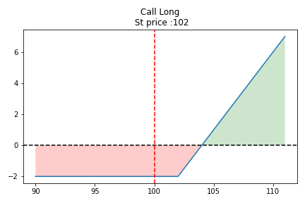
75 |
76 | Green : Profit
Red : Loss
77 |
78 | ### 1.b Input parameters
79 | Strike Price : 450
80 | Spot price : 460
81 | Option type : Put Option
82 | Position : Short
83 | Option Premium : 12.5
84 |
85 | ```python
86 | op.single_plotter(spot=460, strike=460, op_type='p', tr_type='s', op_pr=12.5)
87 | ```
88 | 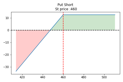
89 |
90 | # 2. multi_plotter()
91 |
92 | Used for plotting a single option
93 | Parameters
94 | ----------
95 | spot: int, float, default: 100
96 | Spot Price
97 |
98 | spot_range: int, float, optional, default: 20
99 | Range of spot variation in percentage
100 |
101 | op_list: list of dictionary
102 | Each dictionary must contiain following keys:
103 |
'strike': int, float, default: 720
104 |
Strike Price
105 |
'tr_type': kind {'b', 's'} default:'b'
106 |
Transaction Type>> 'b': long, 's': short
107 |
'op_pr': int, float, default: 10
108 |
Option Price
109 |
'op_type': kind {'c','p'}, default:'c'
110 |
Opion type>> 'c': call option, 'p':put option
111 |
112 | ### 2.a Default plot : The short strangle
113 |
114 | Options trading that involve:
(a)selling of a slightly out-of-the-money put and
(b)a slightly out-of-the-money call of the same underlying stock and expiration date.
115 |
spot_range=+/-20%
116 |
spot=100
117 |
Option 1:Short call at strike price 110
op_type: 'c','strike': 110 'tr_type': 's', 'op_pr': 2
118 |
Option 2 : Short put at strike price 95
'op_type': 'p', 'strike': 95, 'tr_type': 's', 'op_pr': 6
119 |
120 | ```python
121 | op.multi_plotter()
122 | ```
123 | 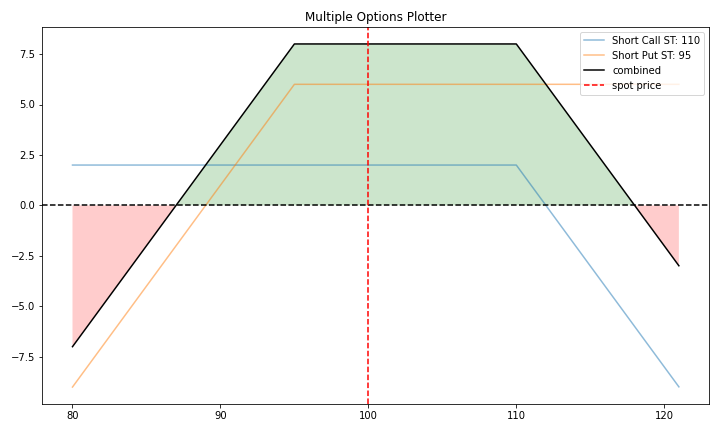
124 |
125 | ### 2.b Example: Iron Condor (Option strategy with 4 options)
126 |
127 | An iron condor is an options strategy consisting of two puts (one long and one short) and two calls (one long and one short), and four strike prices, all with the same expiration date.
128 |
129 | stock currently trading at 212.26 (Spot Price)
130 |
131 | Option 1: Sell a call with a 215 strike, which gives 7.63 in premium
132 | Option 2: Buy a call with a strike of 220, which costs 5.35.
133 | Option 3: Sell a put with a strike of 210 with premium received 7.20
134 | Option 4: Buy a put with a strike of 205 costing 5.52.
135 |
136 | ```python
137 | op1={'op_type': 'c', 'strike': 215, 'tr_type': 's', 'op_pr': 7.63}
138 | op2={'op_type': 'c', 'strike': 220, 'tr_type': 'b', 'op_pr': 5.35}
139 | op3={'op_type': 'p', 'strike': 210, 'tr_type': 's', 'op_pr': 7.20}
140 | op4={'op_type': 'p', 'strike': 205, 'tr_type': 'b', 'op_pr': 5.52}
141 |
142 | op_list=[op1, op2, op3, op4]
143 | op.multi_plotter(spot=212.26,spot_range=10, op_list=op_list)
144 | ```
145 | 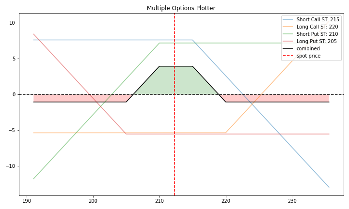
146 |
147 | # 3. yf_plotter()
148 |
149 | Parameters
150 | ----------
151 | ticker: string, default: 'msft' stock ticker for Microsoft.Inc
152 | Stock Ticker
153 | exp: string default: next option expiration date
154 | Option expiration date in 'YYYY-MM-DD' format
155 |
156 | spot_range: int, float, optional, default: 10
157 | Range of spot variation in percentage
158 |
159 | op_list: list of dictionary
160 |
161 | Each dictionary must contiain following keys
162 | 'strike': int, float, default: 720
163 | Strike Price
164 | 'tr_type': kind {'b', 's'} default:'b'
165 | Transaction Type>> 'b': long, 's': short
166 | 'op_type': kind {'c','p'}, default:'c'
167 | Opion type>> 'c': call option, 'p':put option
168 |
169 | ### 3.a Default plot
170 |
171 | Strangle on Microsoft stock
172 | Stock ticker : msft(Microsoft Inc.)
173 | Option 1: Buy Call at Strike Price 250
174 | Option 2: Buy Put option at Strike price 225
175 |
176 | ```python
177 | op.yf_plotter()
178 | ```
179 | 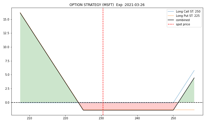
180 |
181 | ### 3.b Example: Strangle on Amazon
182 |
183 | Strangle:
184 | A simultaneous purchase of options to buy and to sell a security or commodity at a fixed price, allowing the purchaser to make a profit whether the price of the security or commodity goes up or down.
185 |
186 | Stock ticker : AMZN(Amazon Inc.)
187 | Option 1: Buy Call at Strike Price 3070
188 | Option 2: Buy Put option at Strike price 3070
189 |
190 | ```python
191 | op_1={'op_type': 'c', 'strike':3070, 'tr_type': 'b'}
192 | op_2={'op_type': 'p', 'strike':3070, 'tr_type': 'b'}
193 | op.yf_plotter(ticker='amzn',
194 | exp='default',
195 | op_list=[op_1, op_2])
196 | ```
197 | 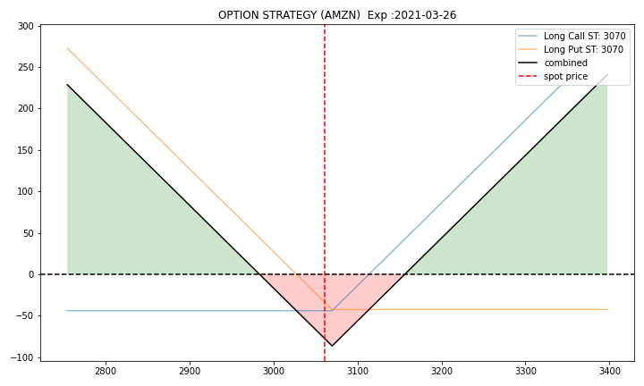
198 |
199 | ## 4. Save figure
200 |
201 | Figure can be saved in the current directory setting save=True
202 | Filename with extension has to be provided as file.
203 | If no filename is provided, the figure will be saved as fig in png format.
204 | ```python
205 | op.single_plotter(save=True,file='simple_option.jpeg')
206 | ```
207 | 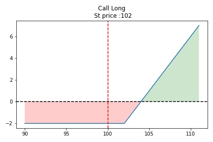
208 |
209 | ## Contributing
210 | Pull requests are welcome. For major changes, please open an issue first to discuss what you would like to change.
211 |
212 | Please make sure to update tests as appropriate.
213 |
214 | ## Content License
215 | [MIT](https://choosealicense.com/licenses/mit/)
216 |
217 | ### Thanks to
218 | [Stackoverflow Community](https://stackoverflow.com/)
219 | [Ran Aroussi](https://github.com/ranaroussi) : [yfinance](https://pypi.org/project/yfinance/)
220 | [Daniel Goldfarb](https://github.com/DanielGoldfarb) : [mplfinance](https://pypi.org/project/mplfinance/)
221 |
222 |
223 | ### Tutorial in Video Format
224 | [](https://youtu.be/EU3L4ziz3nk)
--------------------------------------------------------------------------------
/examples/Black Scholes and Option Greeks.ipynb:
--------------------------------------------------------------------------------
1 | {
2 | "cells": [
3 | {
4 | "cell_type": "markdown",
5 | "metadata": {},
6 | "source": [
7 | "### Import Libraries"
8 | ]
9 | },
10 | {
11 | "cell_type": "code",
12 | "execution_count": 1,
13 | "metadata": {
14 | "ExecuteTime": {
15 | "end_time": "2021-06-30T10:35:14.926145Z",
16 | "start_time": "2021-06-30T10:35:10.314481Z"
17 | }
18 | },
19 | "outputs": [
20 | {
21 | "name": "stderr",
22 | "output_type": "stream",
23 | "text": [
24 | "C:\\Users\\ABCD\\AppData\\Local\\Continuum\\anaconda3\\lib\\site-packages\\statsmodels\\tools\\_testing.py:19: FutureWarning: pandas.util.testing is deprecated. Use the functions in the public API at pandas.testing instead.\n",
25 | " import pandas.util.testing as tm\n"
26 | ]
27 | }
28 | ],
29 | "source": [
30 | "import opstrat as op"
31 | ]
32 | },
33 | {
34 | "cell_type": "markdown",
35 | "metadata": {},
36 | "source": [
37 | "### Declare parameters"
38 | ]
39 | },
40 | {
41 | "cell_type": "code",
42 | "execution_count": 2,
43 | "metadata": {
44 | "ExecuteTime": {
45 | "end_time": "2021-06-30T10:35:19.874732Z",
46 | "start_time": "2021-06-30T10:35:19.859400Z"
47 | }
48 | },
49 | "outputs": [],
50 | "source": [
51 | "K=200 #spot price\n",
52 | "St=208 #current stock price\n",
53 | "r=4 #4% risk free rate\n",
54 | "t=30 #time to expiry, 30 days \n",
55 | "v=20 #volatility \n",
56 | "type='c' #Option type call\n",
57 | "\n",
58 | "bsm=op.black_scholes(K=K, St=St, r=r, t=t, \n",
59 | " v=v, type='c')"
60 | ]
61 | },
62 | {
63 | "cell_type": "markdown",
64 | "metadata": {},
65 | "source": [
66 | "### Option values"
67 | ]
68 | },
69 | {
70 | "cell_type": "code",
71 | "execution_count": 3,
72 | "metadata": {
73 | "ExecuteTime": {
74 | "end_time": "2021-06-30T10:35:26.025687Z",
75 | "start_time": "2021-06-30T10:35:26.010472Z"
76 | }
77 | },
78 | "outputs": [
79 | {
80 | "data": {
81 | "text/plain": [
82 | "{'option value': 10.210518559926442,\n",
83 | " 'intrinsic value': 8,\n",
84 | " 'time value': 2.2105185599264416}"
85 | ]
86 | },
87 | "execution_count": 3,
88 | "metadata": {},
89 | "output_type": "execute_result"
90 | }
91 | ],
92 | "source": [
93 | "bsm['value']"
94 | ]
95 | },
96 | {
97 | "cell_type": "markdown",
98 | "metadata": {},
99 | "source": [
100 | "### Option Greeks"
101 | ]
102 | },
103 | {
104 | "cell_type": "code",
105 | "execution_count": 4,
106 | "metadata": {
107 | "ExecuteTime": {
108 | "end_time": "2021-06-30T10:35:33.797340Z",
109 | "start_time": "2021-06-30T10:35:33.786344Z"
110 | }
111 | },
112 | "outputs": [
113 | {
114 | "data": {
115 | "text/plain": [
116 | "{'delta': 0.7793593241701937,\n",
117 | " 'gamma': 0.024868265088898882,\n",
118 | " 'theta': -0.07559961986526405,\n",
119 | " 'vega': 0.17686037602292404,\n",
120 | " 'rho': 0.12484620893217029}"
121 | ]
122 | },
123 | "execution_count": 4,
124 | "metadata": {},
125 | "output_type": "execute_result"
126 | }
127 | ],
128 | "source": [
129 | "bsm['greeks']"
130 | ]
131 | },
132 | {
133 | "cell_type": "code",
134 | "execution_count": null,
135 | "metadata": {},
136 | "outputs": [],
137 | "source": []
138 | }
139 | ],
140 | "metadata": {
141 | "kernelspec": {
142 | "display_name": "Python 3",
143 | "language": "python",
144 | "name": "python3"
145 | },
146 | "language_info": {
147 | "codemirror_mode": {
148 | "name": "ipython",
149 | "version": 3
150 | },
151 | "file_extension": ".py",
152 | "mimetype": "text/x-python",
153 | "name": "python",
154 | "nbconvert_exporter": "python",
155 | "pygments_lexer": "ipython3",
156 | "version": "3.7.4"
157 | }
158 | },
159 | "nbformat": 4,
160 | "nbformat_minor": 2
161 | }
162 |
--------------------------------------------------------------------------------
/opstrat/__init__.py:
--------------------------------------------------------------------------------
1 | __version__ = "0.1.7"
2 | __author__ = "Abhijith Chandradas"
3 |
4 | from .basic_multi import *
5 | from .basic_single import *
6 | from .yf import *
7 | from .blackscholes import black_scholes
8 | #from .helpers import *
9 |
--------------------------------------------------------------------------------
/opstrat/basic_multi.py:
--------------------------------------------------------------------------------
1 | #multiplotter
2 | import numpy as np
3 | import matplotlib.pyplot as plt
4 | import seaborn as sns
5 |
6 | from .helpers import payoff_calculator, check_optype, check_trtype
7 |
8 | abb={'c': 'Call',
9 | 'p': 'Put',
10 | 'b': 'Long',
11 | 's': 'Short'}
12 |
13 | def multi_plotter(spot_range=20, spot=100,
14 | op_list=[{'op_type':'c','strike':110,'tr_type':'s','op_pr':2,'contract':1},
15 | {'op_type':'p','strike':95,'tr_type':'s','op_pr':6,'contract':1}],
16 | save=False, file='fig.png'):
17 | """
18 | Plots a basic option payoff diagram for a multiple options and resultant payoff diagram
19 |
20 | Parameters
21 | ----------
22 | spot: int, float, default: 100
23 | Spot Price
24 |
25 | spot_range: int, float, optional, default: 20
26 | Range of spot variation in percentage
27 |
28 | op_list: list of dictionary
29 |
30 | Each dictionary must contiain following keys
31 | 'strike': int, float, default: 720
32 | Strike Price
33 | 'tr_type': kind {'b', 's'} default:'b'
34 | Transaction Type>> 'b': long, 's': short
35 | 'op_pr': int, float, default: 10
36 | Option Price
37 | 'op_type': kind {'c','p'}, default:'c'
38 | Opion type>> 'c': call option, 'p':put option
39 | 'contracts': int default:1, optional
40 | Number of contracts
41 |
42 | save: Boolean, default False
43 | Save figure
44 |
45 | file: String, default: 'fig.png'
46 | Filename with extension
47 |
48 | Example
49 | -------
50 | op1={'op_type':'c','strike':110,'tr_type':'s','op_pr':2,'contract':1}
51 | op2={'op_type':'p','strike':95,'tr_type':'s','op_pr':6,'contract':1}
52 |
53 | import opstrat as op
54 | op.multi_plotter(spot_range=20, spot=100, op_list=[op1,op2])
55 |
56 | #Plots option payoff diagrams for each op1 and op2 and combined payoff
57 |
58 | """
59 | x=spot*np.arange(100-spot_range,101+spot_range,0.01)/100
60 | y0=np.zeros_like(x)
61 |
62 | y_list=[]
63 | for op in op_list:
64 | op_type=str.lower(op['op_type'])
65 | tr_type=str.lower(op['tr_type'])
66 | check_optype(op_type)
67 | check_trtype(tr_type)
68 |
69 | strike=op['strike']
70 | op_pr=op['op_pr']
71 | try:
72 | contract=op['contract']
73 | except:
74 | contract=1
75 | y_list.append(payoff_calculator(x, op_type, strike, op_pr, tr_type, contract))
76 |
77 |
78 | def plotter():
79 | y=0
80 | plt.figure(figsize=(10,6))
81 | for i in range (len(op_list)):
82 | try:
83 | contract=str(op_list[i]['contract'])
84 | except:
85 | contract='1'
86 |
87 | label=contract+' '+str(abb[op_list[i]['tr_type']])+' '+str(abb[op_list[i]['op_type']])+' ST: '+str(op_list[i]['strike'])
88 | sns.lineplot(x=x, y=y_list[i], label=label, alpha=0.5)
89 | y+=np.array(y_list[i])
90 |
91 | sns.lineplot(x=x, y=y, label='combined', alpha=1, color='k')
92 | plt.axhline(color='k', linestyle='--')
93 | plt.axvline(x=spot, color='r', linestyle='--', label='spot price')
94 | plt.legend()
95 | plt.legend(loc='upper right')
96 | title="Multiple Options Plotter"
97 | plt.title(title)
98 | plt.fill_between(x, y, 0, alpha=0.2, where=y>y0, facecolor='green', interpolate=True)
99 | plt.fill_between(x, y, 0, alpha=0.2, where=y> 'c': call option, 'p':put option
21 |
22 | spot: int, float, default: 100
23 | Spot Price
24 |
25 | spot_range: int, float, optional, default: 5
26 | Range of spot variation in percentage
27 |
28 | strike: int, float, default: 102
29 | Strike Price
30 |
31 | tr_type: kind {'b', 's'} default:'b'
32 | Transaction Type>> 'b': long, 's': short
33 |
34 | op_pr: int, float, default: 10
35 | Option Price
36 |
37 | save: Boolean, default False
38 | Save figure
39 |
40 | file: String, default: 'fig.png'
41 | Filename with extension
42 |
43 | Example
44 | -------
45 | import opstrat as op
46 | op.single_plotter(op_type='p', spot_range=20, spot=1000, strike=950)
47 | #Plots option payoff diagram for put option with spot price=1000, strike price=950, range=+/-20%
48 |
49 | """
50 |
51 |
52 | op_type=str.lower(op_type)
53 | tr_type=str.lower(tr_type)
54 | check_optype(op_type)
55 | check_trtype(tr_type)
56 |
57 | def payoff_calculator():
58 | x=spot*np.arange(100-spot_range,101+spot_range,0.01)/100
59 |
60 | y=[]
61 | if str.lower(op_type)=='c':
62 | for i in range(len(x)):
63 | y.append(max((x[i]-strike-op_pr),-op_pr))
64 | else:
65 | for i in range(len(x)):
66 | y.append(max(strike-x[i]-op_pr,-op_pr))
67 |
68 | if str.lower(tr_type)=='s':
69 | y=-np.array(y)
70 | return x,y
71 |
72 | x,y=payoff_calculator()
73 | y0=np.zeros_like(x)
74 |
75 | def plotter(x,y):
76 | plt.figure(figsize=(10,6))
77 | sns.lineplot(x=x, y=y)
78 | plt.axhline(color='k', linestyle='--')
79 | plt.axvline(x=spot, color='r', linestyle='--')
80 | title=str(abb[op_type])+' '+str(abb[tr_type])+'\n St price :'+str(strike)
81 | plt.fill_between(x, y, 0, alpha=0.2, where=y>y0, facecolor='green', interpolate=True)
82 | plt.fill_between(x, y, 0, alpha=0.2, where=y> 'b': long, 's': short
41 | 'op_type': kind {'c','p'}, default:'c'
42 | Opion type>> 'c': call option, 'p':put option
43 | 'contracts': int default:1, optional
44 | Number of contracts
45 |
46 | save: Boolean, default False
47 | Save figure
48 |
49 | file: String, default: 'fig.png'
50 | Filename with extension
51 |
52 | Example
53 | -------
54 | op1={'op_type':'c','strike':250,'tr_type':'b', 'contract':1}
55 | op2={'op_type':'p','strike':225,'tr_type':'b','contract':3}
56 |
57 | import opstrat as op
58 | op.yf_plotter(ticker='msft',exp='2021-03-26',spot_range=10, op_list=[op1,op2])
59 |
60 | #Plots option payoff diagrams for each op1 and op2 and combined payoff
61 |
62 | """
63 | #Check input and assigns spot price
64 | spot=check_ticker(ticker)
65 | #Expiry dates
66 | exp_list=yf.Ticker(ticker).options
67 |
68 | x=spot*np.arange(100-spot_range,101+spot_range,0.01)/100
69 | y0=np.zeros_like(x)
70 |
71 |
72 | def check_exp(exp):
73 | """
74 | Check expiry date
75 | """
76 | if exp not in exp_list:
77 | raise ValueError('Option for the given date not available!')
78 |
79 | if exp=='default':
80 | exp=yf.Ticker('msft').options[0]
81 | else:
82 | check_exp(exp)
83 |
84 | def check_strike(df, strike):
85 | if strike not in df.strike.unique():
86 | raise ValueError('Option for the given Strike Price not available!')
87 |
88 | y_list=[]
89 |
90 | for op in op_list:
91 | op_type=str.lower(op['op_type'])
92 | tr_type=str.lower(op['tr_type'])
93 |
94 | check_optype(op_type)
95 | check_trtype(tr_type)
96 |
97 | if(op_type=='p'):
98 | df=yf.Ticker(ticker).option_chain(exp).puts
99 | else:
100 | df=yf.Ticker(ticker).option_chain(exp).calls
101 |
102 | strike=op['strike']
103 | check_strike(df, strike)
104 | op_pr=df[df.strike==strike].lastPrice.sum()
105 | try:
106 | contract=op['contract']
107 | except:
108 | contract=1
109 |
110 | y_list.append(payoff_calculator(x, op_type, strike, op_pr, tr_type, contract))
111 |
112 |
113 | def plotter():
114 | y=0
115 | plt.figure(figsize=(10,6))
116 | for i in range (len(op_list)):
117 | try:
118 | contract=str(op_list[i]['contract'])
119 | except:
120 | contract='1'
121 |
122 | label=contract+' '+str(abb[op_list[i]['tr_type']])+' '+str(abb[op_list[i]['op_type']])+' ST: '+str(op_list[i]['strike'])
123 | sns.lineplot(x=x, y=y_list[i], label=label, alpha=0.5)
124 | y+=np.array(y_list[i])
125 |
126 | sns.lineplot(x=x, y=y, label='combined', alpha=1, color='k')
127 | plt.axhline(color='k', linestyle='--')
128 | plt.axvline(x=spot, color='r', linestyle='--', label='spot price')
129 | plt.legend()
130 | plt.legend(loc='upper right')
131 | title="OPTION STRATEGY ("+str.upper(ticker)+') '+' Exp :'+str(exp)
132 | plt.fill_between(x, y, 0, alpha=0.2, where=y>y0, facecolor='green', interpolate=True)
133 | plt.fill_between(x, y, 0, alpha=0.2, where=y