├── zh
├── hisub.md
├── usage
│ ├── hisub
│ │ └── README.md
│ ├── mini-tools
│ │ └── README.md
│ ├── clinical-tools
│ │ └── README.md
│ ├── advance
│ │ └── README.md
│ └── basic
│ │ └── README.md
├── modules.md
├── development-guides
│ ├── run.md
│ ├── bs4dash.md
│ └── README.md
├── qa.md
├── download
│ ├── README.Rmd
│ └── README.md
└── README.md
├── about.md
├── scripts
├── build_rmd.R
├── download_table.R
└── merge_doc.sh
├── .gitignore
├── usage
├── mini-tools
│ └── README.md
├── clinical-tools
│ └── README.md
└── advance
│ └── README.md
├── .yarnrc.yml
├── contribute.md
├── modules.md
├── package.json
├── download
├── README.Rmd
└── README.md
├── README.md
├── qa.md
├── env.Rmd
├── .vuepress
└── config.js
├── LICENSE
└── development-guides
└── hisub.md
/zh/hisub.md:
--------------------------------------------------------------------------------
1 | # Hisub
2 |
3 | Content...
4 |
--------------------------------------------------------------------------------
/zh/usage/hisub/README.md:
--------------------------------------------------------------------------------
1 | # Hisub
2 |
3 | Content...
4 |
--------------------------------------------------------------------------------
/zh/modules.md:
--------------------------------------------------------------------------------
1 | # 模块简介
2 |
3 | ## 文件系统
4 |
5 | ## 可视化系统
6 |
7 | ## 其他任务
8 |
9 |
--------------------------------------------------------------------------------
/about.md:
--------------------------------------------------------------------------------
1 | # About Us
2 |
3 | Hiplot team members mainly come from the [openbiox](https://github.com/openbiox) communitiy.
4 |
--------------------------------------------------------------------------------
/scripts/build_rmd.R:
--------------------------------------------------------------------------------
1 | #!/usr/bin/env Rscript
2 | knitr::knit("env.Rmd", 'env.md')
3 | knitr::knit("download/README.Rmd", 'download/README.md')
4 | knitr::knit("zh/download/README.Rmd", 'zh/download/README.md')
5 |
6 |
--------------------------------------------------------------------------------
/zh/usage/mini-tools/README.md:
--------------------------------------------------------------------------------
1 | # 小工具箱
2 |
3 | ## [简易三线表](/mini-tools/easy-booktab)
4 |
5 | - 简介
6 |
7 | 基于 R gtsummary 自动整理发表级别表格数据。
8 | ## [颜色提取工具](/mini-tools/extract-colors)
9 |
10 | - 简介
11 |
12 | 可以用于从图片中识别颜色生成色板。
13 | ## [PDF Collage](/mini-tools/pdf-collage)
14 |
15 | - 简介
16 |
17 | 可以自由的调整和组合多个图片和 PDF 文件作为发表级别排版。
18 |
--------------------------------------------------------------------------------
/.gitignore:
--------------------------------------------------------------------------------
1 | .DS_Store
2 | .Rproj.user
3 | .Rhistory
4 | .RData
5 | .Ruserdata
6 | node_modules
7 | dist
8 | .vuepress/dist
9 |
10 | # local env files
11 | .env.local
12 | .env.*.local
13 |
14 | # Log files
15 | npm-debug.log*
16 | yarn-debug.log*
17 | yarn-error.log*
18 |
19 | # Editor directories and files
20 | .idea
21 | .vscode
22 | *.suo
23 | *.ntvs*
24 | *.njsproj
25 | *.sln
26 | *.sw*
27 |
28 | env.md
29 | .yarn
30 |
--------------------------------------------------------------------------------
/usage/mini-tools/README.md:
--------------------------------------------------------------------------------
1 | # Mini Tools
2 |
3 | ## [Easy Booktab](/mini-tools/easy-booktab)
4 |
5 | - Introduction
6 |
7 | It can be used to create publication-ready analytical and summary tables based on gtsummary R package.
8 | ## [Extract Colors](/mini-tools/extract-colors)
9 |
10 | - Introduction
11 |
12 | Can be used to extract the colors from images.
13 | ## [PDF Collage](/mini-tools/pdf-collage)
14 |
15 | - Introduction
16 |
17 | Can be used to freely arrange amd combine multiple image or PDF files for publication layout.
18 |
--------------------------------------------------------------------------------
/.yarnrc.yml:
--------------------------------------------------------------------------------
1 | packageExtensions:
2 | 'vuepress@*':
3 | dependencies:
4 | '@vuepress/shared-utils': '*'
5 | 'vue-server-renderer@2.7.14':
6 | dependencies:
7 | 'vue': '^2.7.14'
8 | '@vuepress/shared-utils@*':
9 | dependencies:
10 | 'markdown-it-emoji': '*'
11 | 'lru-cache': '*'
12 | '@vue/component-compiler-utils': '*'
13 | '@vuepress/markdown-loader@*':
14 | dependencies:
15 | '@vuepress/shared-utils': '*'
16 | '@vuepress/core@*':
17 | dependencies:
18 | 'escape-html': '*'
19 | nodeLinker: 'node-modules'
--------------------------------------------------------------------------------
/contribute.md:
--------------------------------------------------------------------------------
1 | # How to contribute
2 |
3 | You can join the user community first: [Discord](https://discord.gg/vX6tSax) or [QQ Group](https://docs.qq.com/doc/DS1RJcVZXbHZQT2lV).
4 |
5 | All feedback and visualization scripts can be shared on the user community. We will respond instantly and update the corresponding visualization plugin . For the security of our website, we will do not share the web service code publicly, and only the core team can access and modified it. If you want to join our core team, you can also feel free to contact us: admin@hiplot.org.
6 |
7 | Besides, We will periodically hold offline community and core team meetings at Shanghai, China, if you are interested you can apply to participate.
8 |
--------------------------------------------------------------------------------
/zh/usage/clinical-tools/README.md:
--------------------------------------------------------------------------------
1 | # 临床工具箱
2 |
3 | ## [AML-G1-G8](/clinical-tools/clinaml-gep2)
4 |
5 | - 简介
6 |
7 | 预测 AML 基因表达亚型。
8 |
9 | G1: PML::RARA
10 |
11 | G2: CBFB::MYH11
12 |
13 | G3: RUNX1::RUNXT1
14 |
15 | G4: biCEBPA/-like
16 |
17 | G5: myelodysplasia-related/-like
18 |
19 | G6: HOX-committed
20 |
21 | G7: HOX-primitive
22 |
23 | G8: HOX-mixed## [AML-G1-G6](/clinical-tools/clinaml-gep)
24 |
25 | - 简介
26 |
27 | 集成模型用于预测 AML 基因表达亚型。
28 |
29 | G1: PML-RARA
30 |
31 | G2: CBFB-MYH11
32 |
33 | G3: RUNX1-RUNXT1
34 |
35 | G4: Bialleic CEBPA
36 |
37 | G5: ...
38 |
39 | G6: NPM1/KMT2A/NUP98...
40 |
41 | - 额外参数
42 |
43 | 数据标准化方法:deseq2 vst 或 log2 (tpm + 1)
44 |
45 | 模型:xgboost 或 autogluon
46 |
47 | - 其他说明
48 |
49 | 模型训练数据的基因名基于 hg38 GENCODE v34 基因注释文件
50 |
51 | 'label' 行只用于检查最终结果的准确度,输入程序后会自动删除
--------------------------------------------------------------------------------
/zh/development-guides/run.md:
--------------------------------------------------------------------------------
1 | # 工具调试方案
2 |
3 | ## 调试方式
4 |
5 | Hiplot 开源及初级开发者主要通过以下方式进行工具调试:
6 |
7 | 1. 克隆 Hiplot 的代码仓库至同一级目录:[plugins-open](https://github.com/hiplot/plugins-open), [plugins-developer](https://github.com/hiplot/plugins-developer);
8 | 2. Vue.js 前端 + R/其他后端程序的工具:进入该工具目录(toolname)运行该工具目录下的 `run.sh` 脚本直接输出结果。如果希望更新优化参数和脚本,可以修改工具目录下的 `data.json` 和 `plot.R` 完成后台脚本更新、`ui.json` 完成前端页面更新。
9 | 3. Shiny 应用:直接使用 Rstudio 进行调试开发;
10 | 4. 纯前端应用:直接使用 VS Code + Chrome 进行实时调试开发。
11 |
12 |
13 | Hiplot 高阶开发者主要通过以下方式进行工具调试:
14 |
15 | 1. 克隆 Hiplot 高阶开发者核心仓库;
16 | 2. Vue.js 前端 + R/其他后端程序的工具:进入核心仓库,并运行该目录下的 `run_debug.R` 脚本完成工具执行:`Rscript run_debug.R -c toolname/data.json -i toolname/data.txt -t toolname -m modulename --enableExample`。如果希望更新优化参数和脚本,可以修改对应工具目录下的 `data.json` 和 `plot.R` 完成后台脚本更新、`ui.json` 完成前端页面更新;
17 | 3. Shiny 应用:直接使用 Rstudio 进行调试;
18 | 4. 纯前端应用:直接使用 VS Code + Chrome 进行实时调试开发。
19 |
20 | ## 注意事项
21 |
22 | 开源及初级开发者仓库和高阶开发者仓库开发格式(Vue.js 前端 + R/其他后端程序的工具)存在一定差异,后者针对生产环境进行了一系列额外优化,且无需在 `plot.R` 脚本中加载 `lib.R`、`head.R` 以及 `foot.R`,以加速应用执行速度。
23 |
24 | 开源及初级开发者仓库工具会在经过修改和优化后将被整合进入高阶开发者仓库,同时完成生产环境上线。
25 |
--------------------------------------------------------------------------------
/usage/clinical-tools/README.md:
--------------------------------------------------------------------------------
1 | # Clinial Tools
2 |
3 | ## [AML-G1-G8](/clinical-tools/clinaml-gep2)
4 |
5 | - Introduction
6 |
7 | Predictiton of the GEP-defined AML subtypes.
8 |
9 | G1: PML::RARA
10 |
11 | G2: CBFB::MYH11
12 |
13 | G3: RUNX1::RUNXT1
14 |
15 | G4: biCEBPA/-like
16 |
17 | G5: myelodysplasia-related/-like
18 |
19 | G6: HOX-committed
20 |
21 | G7: HOX-primitive
22 |
23 | G8: HOX-mixed## [AML-G1-G6](/clinical-tools/clinaml-gep)
24 |
25 | - Introduction
26 |
27 | Bagging models to predict the GEP-defined AML subtypes.
28 |
29 | G1: PML-RARA
30 |
31 | G2: CBFB-MYH11
32 |
33 | G3: RUNX1-RUNXT1
34 |
35 | G4: Bialleic CEBPA
36 |
37 | G5: ...
38 |
39 | G6: NPM1/KMT2A/NUP98...
40 |
41 | - Extra parameters
42 |
43 | Data normalization method: deseq2 vst or log2 (tpm + 1)
44 |
45 | Model: xgboost or autogluon
46 |
47 | - Other notes
48 |
49 | Gene symbols of models are based on the hg38 GENCODE v34 gene annotation file
50 |
51 | 'label' row is only used to check results for users and will be automatically removed in the program
--------------------------------------------------------------------------------
/scripts/download_table.R:
--------------------------------------------------------------------------------
1 | library(data.table)
2 | library(stringr)
3 | library(jsonlite)
4 |
5 | download_table <- function (x, version_field) {
6 | download_dir <- getOption("hiplot.download_dir")
7 | latest <- read_json(file.path(download_dir, "last_update"))[[version_field]]
8 | dest <- file.path(download_dir, x, paste0("v", latest))
9 | md5sum <- fread(cmd = sprintf("cat %s/md5sum | sed 's; ;\t;'", dest),
10 | sep = "\t", data.table = FALSE, header = FALSE)
11 | base_dir <- sprintf("https://download.hiplot.cn/download/%s/v%s", x, latest)
12 | finfo <- file.info(file.path(dest, md5sum[,2]))
13 | md5sum[,"Date"] <- as.Date(finfo$mtime, "%d%b%Y")
14 | md5sum[,"Size"] <- sapply(finfo$size, function(x) {
15 | utils:::format.object_size(x, "auto")
16 | })
17 | md5sum[,"URL"] <- file.path(base_dir, basename(md5sum[,2]))
18 | md5sum[,"File"] <- basename(md5sum[,2])
19 | md5sum <- md5sum[md5sum$File != "md5sum",]
20 | colnames(md5sum)[1] <- "MD5"
21 | md5sum[,"File"] <- sprintf("[%s](%s)", md5sum[,"File"], md5sum[,"URL"])
22 | md5sum <- md5sum[,c("File", "Size", "Date", "MD5")]
23 | knitr::kable(md5sum)
24 | }
25 |
--------------------------------------------------------------------------------
/scripts/merge_doc.sh:
--------------------------------------------------------------------------------
1 | echo "# Basic Module
2 | " > usage/basic/README.md
3 | cat ../plugins/private/basic/r/*/README.md >> usage/basic/README.md
4 |
5 | echo "# 基础模块
6 | " > zh/usage/basic/README.md
7 | cat ../plugins/private/basic/r/*/README-zh_cn.md >> zh/usage/basic/README.md
8 |
9 | echo "# Advanced Module
10 | " > usage/advance/README.md
11 | cat ../plugins/private/advance/scripts/r/*/README.md >> usage/advance/README.md
12 |
13 | echo "# 进阶模块
14 | " > zh/usage/advance/README.md
15 | cat ../plugins/private/advance/scripts/r/*/README-zh_cn.md >> zh/usage/advance/README.md
16 |
17 | echo "# Mini Tools
18 | " > usage/mini-tools/README.md
19 | cat ../plugins/private/mini-tools/r/*/README.md >> usage/mini-tools/README.md
20 |
21 | echo "# 小工具箱
22 | " > zh/usage/mini-tools/README.md
23 | cat ../plugins/private/mini-tools/r/*/README-zh_cn.md >> zh/usage/mini-tools/README.md
24 |
25 | echo "# Clinial Tools
26 | " > usage/clinical-tools/README.md
27 | cat ../plugins/private/clinical-tools/r/*/README.md >> usage/clinical-tools/README.md
28 |
29 | echo "# 临床工具箱
30 | " > zh/usage/clinical-tools/README.md
31 | cat ../plugins/private/clinical-tools/r/*/README-zh_cn.md >> zh/usage/clinical-tools/README.md
32 |
--------------------------------------------------------------------------------
/zh/usage/advance/README.md:
--------------------------------------------------------------------------------
1 | # 进阶模块
2 |
3 | ## [AGFusion](/advance/agfusion)
4 |
5 | 用于在一维蛋白和基因组水平可视化融合基因结构模式。
6 |
7 | - 数据表格(四列):
8 |
9 | gene5 | 5' 基因
10 |
11 | gene3 | 3' 基因
12 |
13 | breakpoint5 | 5‘ 断点
14 |
15 | breakpoint3 | 3‘ 断点
16 |
17 | - 额外参数
18 |
19 | 参考基因版本 | 基因组版本号:hg38 或 hg19
20 |
21 | 输出野生型基因 | 同时输出野生型基因结构
22 | ## [Chromsomes-Scatter](/advance/chromsomes-scatter)
23 |
24 | 染色体坐标可视化数值分布。
25 | ## [ClusterProfiler GO/KEGG](/advance/clusterprofiler-go-kegg)
26 |
27 | 详细参数见 [ClusterProfiler Books](https://hiplot-academic.com/books-static/clusterprofiler-book).
28 |
29 | 注意:
30 |
31 | - `KEGG DB` 参数可以输入 .rds 格式的文件或者物种名 (如 hsa 和 rno) (示例 2)。
32 | - 所有数据列都将独立进行富集分析
33 | - 如果绘图结果中存在灰色空白区,说明未显著富集到条目,可能需要调整 P 或 Q 阈值来纳入更多条目
34 | ## [Cola](/advance/cola)
35 |
36 | - 简介
37 |
38 | 共识聚类分析(Consensus clustering)基于 cola 框架。
39 | ## [DiscoverMutTest](/advance/discover-mut-test)
40 |
41 | 用于分析癌症基因突变的共存互斥性。
42 | ## [Fusion-Circlize](/advance/fusion-circlize)
43 |
44 | 使用染色体圈图可视化融合基因。
45 | ## [GGMSA](/advance/ggmsa)
46 |
47 | 可以基于 ggplot2 语法可视化多重序列比对结果。
48 | ## [GGtree-MSA](/advance/ggtree-msa)
49 |
50 | 可以用于可视化进化树和多重序列比对结果。
51 | ## [GISTIC2](/advance/gistic2)
52 |
53 | ⚠️注意:如果程序没有发现 overlap 相关的错误,请不要使用预处理相关的 2 个参数,请保持保持它们为默认值。
54 |
55 | 新增加的 2 个参数不属于 GISTIC2 软件本身,它们被设计用来处理 GISTIC2 报告 Overlap 相关错误:
56 |
57 | - 预处理 Overlap 片段:激活预处理。
58 | - 预处理最少探针数:如果预处理被激活,该参数可以用来过滤掉小于该参数值的拷贝数片段。 ## [染色体热图](/advance/ideogram-heat)
59 |
60 | 染色体坐标可视化数值分布。
61 | ## [突变全景图](/advance/oncoplot)
62 |
63 | - 简介
64 |
65 | 突变全景图可以用于展示癌症队列基因组突变概貌。
66 | ## [Pathview](/advance/pathview)
67 |
68 | 计算平均表达量,然后在 KEGG 通路中进行展示。
69 |
--------------------------------------------------------------------------------
/zh/qa.md:
--------------------------------------------------------------------------------
1 | # 常见问题
2 |
3 | ## 账户与联系
4 |
5 | **1. 如何联系我们?**
6 |
7 | - 邮件联系: admin@hiplot.org
8 | - 右上角点击用户反馈按钮,发送对应主题信息
9 | - 在 https://github.com/hiplot/gold/issues 仓库发帖
10 | - 加入 Hiplot [Discord 社群](https://discord.gg/vX6tSax)或[微信社群](https://docs.qq.com/doc/DS09na3NVYk9OcHVp)
11 |
12 | **2. 注册或找回密码后未收到对应回执邮件怎么办?**
13 |
14 | - 查看垃圾邮箱
15 | - 更换邮箱进行注册
16 | - 邮件联系 admin@hiplot.org
17 |
18 | **3. 如何登陆 Hiplot Tiny RSS server?**
19 |
20 | 访问 https://hiplot.cn/ttrss, 使用 Hiplot 邮箱和默认密码 'public' 进行登录。
21 |
22 | **4. 如何登陆 Hiplot Galaxy 镜像服务?**
23 |
24 | 访问 https://galaxy.hiplot.cn, 使用 Hiplot 邮箱和默认密码 'public' 进行登录。
25 |
26 | ## 数据导入
27 |
28 | **1. 数据表只展示 5000 行和 99 列?**
29 |
30 | 背后真实的数据行和列数是完整的。粘贴和导入的数据都会被完整提交,并不会截断数据。可以点击导出按钮确认。
31 |
32 | **2. 导入示例数据后,窗口滚动条不见了?**
33 |
34 | 将鼠标移出表格即可。
35 |
36 | **3. 无法从 Excel 复制数据导入数据表?**
37 |
38 | 复制粘贴前需要点击对应数据表之后才可以将内容通过复制粘贴导入。
39 |
40 | ## 应用使用方法
41 |
42 | **1. matrix-bubble 数据展示不全怎么办?**
43 |
44 | 修改颜色主题,尝试使用不同主题,或选择 custom 输入自定义颜色,输入的颜色数量应大于对应的分类变量长度。
45 |
46 | **2. 如果出现 Error: Insufficient values in manual scale 报错并无法出图怎么办?**
47 |
48 | 修改颜色主题,尝试使用不同主题,或选择 custom 输入自定义颜色,输入的颜色数量应大于对应的分类变量长度。
49 |
50 | **3. WGCNA 分析任务一直未完成怎么办?**
51 |
52 | Hiplot 仅提供单线程模式进行 WGCNA 分析,所以大数据集将会无法在短时间内完成计算,建议对基因进行初步筛选:如变异很小的基因、去掉非编码基因等。另外,我们的代码已经尽可能的优化了分析参数,但由于 WGCNA 分析本身涉及的步骤和算法相对复杂,对于发表级别的最优共表达网络构建,我们仍然建议用户在本地构建分析环境,并参考 WGCNA 官网的教程逐步完成。通过调整不同参数来评估数据结果稳定性,并获得可解释的具有真实生物学意义的结果。
53 |
54 | **4. GSEA 分析出现报错: Bad format - expect ncols: 2 but found: XX on line?**
55 |
56 | 检查 cls 文件前两行,删除掉末尾的所有空字符。
57 |
58 | **5. 弦图(chord)每次绘图的颜色都不一样怎么办?**
59 |
60 | 修改颜色参数,默认为 random,所以会每次生成不一样的颜色。
61 |
62 | **6. GO/KEGG 出现报错:ERROR [2021-03-12 15:18:33] Error in ans[ypos] <- rep(yes, length.out = len)[ypos]: replacement has length zero**
63 |
64 | 调节 P Value / Q Value 阈值到 1。
65 |
66 | **7. GO/KEGG 有灰色空白区?**
67 |
68 | 说明按照阈值设定未富集到条目,可按照 Q12 进行相同处理。
69 |
70 | **8. 如何设置自定义颜色?**
71 |
72 | 改变颜色画板值为 'custom',然后在自定义颜色字段输入 16 进制颜色代码, 如 #000000。多个 16 进制颜色用空格或逗号分隔。
73 |
--------------------------------------------------------------------------------
/zh/download/README.Rmd:
--------------------------------------------------------------------------------
1 | # Download
2 |
3 | ```{r setup, include=FALSE}
4 | knitr::opts_chunk$set(echo = TRUE)
5 | ```
6 |
7 | ## 桌面客户端
8 |
9 | 我们基于 [Electron](https://www.electronjs.org/) 构建了 Hiplot 的桌面客户端。示例数据和 UI 组件将在特定版本下被固定。
10 |
11 | 最新版本:
12 |
13 | ```{r echo = FALSE}
14 | source("../../scripts/download_table.R")
15 | download_table("desktop", "versionDesktop")
16 | ```
17 |
18 | 其他桌面版本: [这里](https://download.hiplot.cn/download/desktop/)
19 |
20 | ## hctl
21 |
22 | hctl 是 Hiplot 网站的命令行程序. 它可以让用户在命令行环境下使用 Hiplot 网站的绘图系统。
23 |
24 | 最新发布版本 (v0.1.7):
25 |
26 | ```{r echo = FALSE}
27 | download_table("hctl", "versionTerminal")
28 | ```
29 |
30 | 其他 hctl 版本: [这里](https://hiplot.cn/download/hctl)
31 |
32 | 使用 hctl 进行绘图之前,用户需要使用 `hctl login` 命令获得 Hiplot 的服务授权。 登录成功后,即可使用 `hctl plot` 命令进行绘图:输入数据为一个 JSON 格式的参数文件和/或一个/多个数据表。
33 |
34 | 示例输入 [demo.tar.gz](https://hiplot.cn/download/hctl/_demo.tar.gz)。
35 |
36 | ```bash
37 | ## Linux 64 Demo
38 | mkdir /tmp/hiplot
39 | cd /tmp/hiplot
40 | wget https://hiplot.cn/download/hctl/v0.1.7/hctl_0.1.7_Linux_64-bit.tar.gz
41 | wget https://hiplot.cn/download/hctl/_demo.tar.gz
42 |
43 | tar -xzvf hctl_0.1.7_Linux_64-bit.tar.gz
44 | tar -xzvf _demo.tar.gz
45 |
46 | ./hctl login
47 |
48 | # 只输入本地数据文件
49 | ./hctl plot -c _demo/heatmap/config.json -t heatmap -d _demo/heatmap/countData.txt,_demo/heatmap/sampleInfo.txt,_demo/heatmap/geneInfo.txt -o /tmp/hiplot-pure-data-mode
50 |
51 | # 只使用远程服务器文件
52 | ./hctl plot -c _demo/heatmap/config2.json -t heatmap -o /tmp/hiplot-pure-remote-data-mode
53 |
54 | # 混合使用本地数据和远程服务器文件
55 | ./hctl plot -c _demo/heatmap/config3.json -t heatmap -d _demo/heatmap/countData.txt,,_demo/heatmap/geneInfo.txt -o /tmp/hiplot-mixed-mode
56 |
57 | # 使用 Hiplot 网站导出的参数文件
58 | ./hctl plot -p _demo/heatmap/params.json -t heatmap -o /tmp/hiplot-params-mode
59 |
60 | # hiplot config 和 plot 命令联合
61 | ## 展示 hctl 支持的网页插件
62 | hctl config -l
63 | ## 下载 basic/tsne 插件配置文件
64 | hctl config basic/tsne
65 | ## 绘制 tsne 图形
66 | hctl plot -p basic-tsne-params.json -o /tmp/hiplot-tsne
67 | ```
68 |
69 | ### 命令行主程序
70 |
71 | ```{bash message=FALSE, warning=FALSE, echo=FALSE}
72 | cd /tmp
73 | hctl -h
74 | ```
75 |
76 | ### 绘图子程序
77 |
78 | ```{bash message=FALSE, warning=FALSE, echo=FALSE}
79 | cd /tmp
80 | hctl plot -h
81 | ```
82 |
--------------------------------------------------------------------------------
/modules.md:
--------------------------------------------------------------------------------
1 | # Summary of modules
2 |
3 | All available modules of Hiplot are listed in left panel of the website.
4 |
5 | - [Home](https://hiplot.cn)
6 | - [Basic Module](https://hiplot.cn/basic)
7 | - [Advanced Module](https://hiplot.cn/advance)
8 | - [Clinical Tools](https://hiplot.cn/clinical-tools)
9 | - [Mini Tools](https://hiplot.cn/mini-tools)
10 | - [Books](https://hiplot.cn/books)
11 | - [File Manager](https://hiplot.cn/file-manager)
12 | - [Account Center](https://hiplot.cn/account-center)
13 | - [Developer Center](https://hiplot.cn/developer-center)
14 | - [Developer Wall](https://hiplot.cn/developer-wall)
15 |
16 | Now, the major functions of Hiplot are provided by [Basic Module](https://hiplot.cn/basic), [Advanced Module](https://hiplot.cn/advance), and [Mini Tools](https://hiplot.cn/mini-tools). All applications are displayed as card matrices in the module of Hiplot. The application card contains the basic information including the name, one-sentence introduction, scores, and tags.
17 |
18 | 
19 |
20 | ## Basic module
21 |
22 | The basic module can be used to do basic scientific visualization tasks.
23 |
24 | ## Advanced Module
25 |
26 | The advanced module can be used to do more complex tasks.
27 |
28 | ## File Manager
29 |
30 | Users can upload the files using the web interface and RESTful APIs:
31 |
32 | 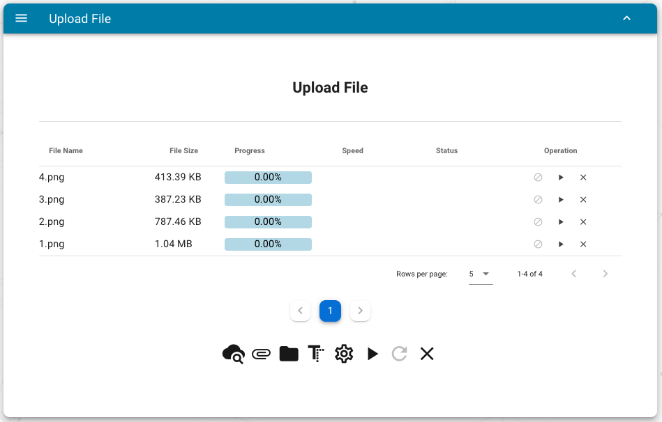
33 |
34 | The meaning of the bottom buttons:
35 |
36 | - view cloud files
37 | - add one local file
38 | - add all files in one directory
39 | - add paste data as a new file
40 | - change default destination directory name (default `upload`)
41 | - start to upload all added files
42 | - retry all failed upload tasks
43 | - remove all upload tasks
44 |
45 | 
46 |
47 | After successfully uploaded, users can manage their files via the following interface:
48 |
49 | 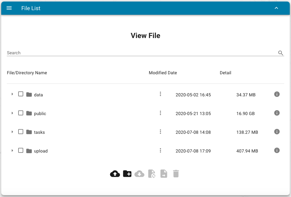
50 |
51 | Users can view, edit, copy, move, and delete all files excluding the `public` directory, which is a soft link for demo plots.
52 |
53 | The meaning of the bottom buttons:
54 |
55 | - upload file
56 | - create a new directory
57 | - download selected directories and files
58 | - copy selected directories and files to another directory
59 | - move selected directories and files to another directory
60 | - delete selected directories and files
61 |
--------------------------------------------------------------------------------
/package.json:
--------------------------------------------------------------------------------
1 | {
2 | "private": true,
3 | "version": "0.2.0",
4 | "name": "docs",
5 | "description": "docs of hiplot",
6 | "scripts": {
7 | "dev": "node --max_old_space_size=8192 ./node_modules/vuepress/cli.js dev .",
8 | "build": "./scripts/merge_doc.sh && ./scripts/build_rmd.R && vuepress build .",
9 | "show-help": "vuepress --help"
10 | },
11 | "repository": {
12 | "type": "git",
13 | "url": "git+https://github.com/hiplot/docs"
14 | },
15 | "keywords": [
16 | "documentation",
17 | "vue",
18 | "generator"
19 | ],
20 | "author": "Hiplot team",
21 | "bugs": {
22 | "url": "https://github.com/hiplot/gold/issues"
23 | },
24 | "homepage": "https://hiplot.cn/docs",
25 | "devDependencies": {
26 | "@hapi/hoek": "^9.2.1",
27 | "@vue/component-compiler-utils": "^3.3.0",
28 | "@vuepress/plugin-back-to-top": "^1.9.7",
29 | "@vuepress/plugin-google-analytics": "^1.9.7",
30 | "@vuepress/plugin-i18n-ui": "^1.0.0-alpha.32",
31 | "@vuepress/plugin-medium-zoom": "^1.9.7",
32 | "@vuepress/plugin-notification": "^1.0.0-alpha.32",
33 | "@vuepress/plugin-pwa": "^1.9.7",
34 | "@vuepress/shared-utils": "^1.9.8",
35 | "@vuepress/theme-default": "^1.9.8",
36 | "acorn": "^8.7.0",
37 | "ansi-regex": "^6.0.1",
38 | "browserslist": "^4.20.2",
39 | "cache-loader": "^4.1.0",
40 | "color-string": "^1.9.0",
41 | "dns-packet": "^5.3.1",
42 | "dot-prop": "^7.2.0",
43 | "elliptic": "^6.5.4",
44 | "escape-html": "^1.0.3",
45 | "glob-parent": "^6.0.2",
46 | "hash-sum": "^2.0.0",
47 | "http-proxy": "^1.18.1",
48 | "ini": "^3.0.0",
49 | "is-svg": "^4.3.2",
50 | "json-schema": "0.4.0",
51 | "kind-of": "^6.0.3",
52 | "lodash": "^4.17.21",
53 | "lodash.uniq": "^4.5.0",
54 | "lru-cache": "^7.14.1",
55 | "markdown-it-emoji": "^2.0.2",
56 | "node-forge": "^1.3.1",
57 | "normalize-url": "^7.0.3",
58 | "nth-check": "^2.0.1",
59 | "path-parse": "^1.0.7",
60 | "postcss": "^8.4.12",
61 | "prismjs": "^1.28.0",
62 | "serialize-javascript": "^6.0.0",
63 | "set-value": "^4.0.1",
64 | "sockjs": "^0.3.24",
65 | "ssri": "^9.0.0",
66 | "tar": "^6.1.11",
67 | "url-parse": "^1.5.10",
68 | "vuepress": "^1.9.7",
69 | "vuepress-plugin-flowchart": "^1.5.0",
70 | "webpack": "3",
71 | "websocket-extensions": "^0.1.4",
72 | "ws": "^8.5.0",
73 | "y18n": "^5.0.8",
74 | "yargs-parser": "^21.0.1"
75 | }
76 | }
77 |
--------------------------------------------------------------------------------
/download/README.Rmd:
--------------------------------------------------------------------------------
1 | # Download
2 |
3 | ```{r setup, include=FALSE}
4 | knitr::opts_chunk$set(echo = TRUE)
5 | ```
6 |
7 | ## Desktop Client
8 |
9 | We build the desktop client of Hiplot (ORG) based on the [Electron](https://www.electronjs.org/). The demo data and UI components are fixed in the desktop client under the given version.
10 |
11 | Latest release version:
12 |
13 | ```{r echo = FALSE}
14 | source("../scripts/download_table.R")
15 | download_table("desktop", "versionDesktop")
16 | ```
17 |
18 | Other releases of desktop client: [here](https://hiplot.cn/download/desktop)
19 |
20 | ## hctl
21 |
22 | hctl is the command-line client of Hiplot (ORG) website. It can be used to draw plots without the web environment.
23 |
24 | Latest release version (v0.1.7):
25 |
26 | ```{r echo = FALSE}
27 | download_table("hctl", "versionTerminal")
28 | ```
29 |
30 | Other releases of hctl: [here](https://hiplot.cn/download/hctl)
31 |
32 | It is required to login Hiplot (ORG) server first using the `hctl login` command. `hctl plot` command can be used to draw plots by using the parameter file and data files.
33 |
34 | Demo input files of hctl can be download from here: [demo.tar.gz](https://hiplot.cn/download/hctl/_demo.tar.gz).
35 |
36 | ```bash
37 | ## Linux 64 Demo
38 | mkdir /tmp/hiplot
39 | cd /tmp/hiplot
40 | wget https://hiplot.cn/download/hctl/v0.1.7/hctl_0.1.7_Linux_64-bit.tar.gz
41 | wget https://hiplot.cn/download/hctl/_demo.tar.gz
42 |
43 | tar -xzvf hctl_0.1.7_Linux_64-bit.tar.gz
44 | tar -xzvf _demo.tar.gz
45 |
46 | hctl login
47 |
48 | # only input data files
49 | hctl plot -c _demo/heatmap/config.json -t heatmap -d _demo/heatmap/countData.txt,_demo/heatmap/sampleInfo.txt,_demo/heatmap/geneInfo.txt -o /tmp/hiplot-pure-data-mode
50 |
51 | # only use remote files
52 | hctl plot -c _demo/heatmap/config2.json -t heatmap -o /tmp/hiplot-pure-remote-data-mode
53 |
54 | # mixed usage
55 | hctl plot -c _demo/heatmap/config3.json -t heatmap -d _demo/heatmap/countData.txt,,_demo/heatmap/geneInfo.txt -o /tmp/hiplot-mixed-mode
56 |
57 | # hiplot exported params
58 | hctl plot -p _demo/heatmap/params.json -t heatmap -o /tmp/hiplot-params-mode
59 |
60 | # hiplot config 和 plot 命令联合
61 | ## show hctl supported plugins
62 | hctl config -l
63 | ## download basic/tsne params
64 | hctl config basic/tsne
65 | ## draw tsne graphics
66 | hctl plot -p basic-tsne-params.json -o /tmp/hiplot-tsne
67 | ```
68 |
69 | ### Main Interface
70 |
71 | ```{bash message=FALSE, warning=FALSE, echo=FALSE}
72 | cd /tmp
73 | hctl -h
74 | ```
75 |
76 | ### Plot Interface
77 |
78 | ```{bash message=FALSE, warning=FALSE, echo=FALSE}
79 | cd /tmp
80 | hctl plot -h
81 | ```
82 |
--------------------------------------------------------------------------------
/README.md:
--------------------------------------------------------------------------------
1 | # Overview
2 |
3 |  4 |
5 | [English Version](./) | [中文版](./zh)
6 |
7 | Interactive visualization and personalized in-depth interpretation of multi-dimensional scientific research data have become one of the major challenges for quantitative researches.
8 |
9 | In recent years, with the development of various cloud computing platforms (such as Galaxy and DNAnexus in the biomedical field) and IT hardware and software (such as distributed computing, container technology, package manager, workflow language, etc.), junior researchers can easily obtain the upstream result. Moreover, when the upstream analysis process of conventional omics data tends to be stable and perfect, the customization and variability of the upstream analysis process have been greatly reduced. The visualization and personalized in-depth interpretation in the downstream process of data analysis have become the biggest challenge facing current users:
10 |
11 | 1. Most of the visualization software or methods developed by the open source user community have not been well integrated under a unified user interface;
12 | 2. There is no active collaborative community for the visualization of scientific research data in China, and the "** Draw Group" has become one of the few choices for primary scientific research users;
13 | 3. There is a lack of core data visualization software and platforms similar to Graphpad and MATLAB in China. After being banned by the United States, they can only spend additional costs to migrate the process or start over;
14 | 4. There are several disadvantages of existing platforms and tools: the user interface is not beautiful enough; lack of the Chinese and English support; it is still difficult to get started; the file Manager of some platforms is not convenient; users cannot actively participate in platform development.
15 |
16 | 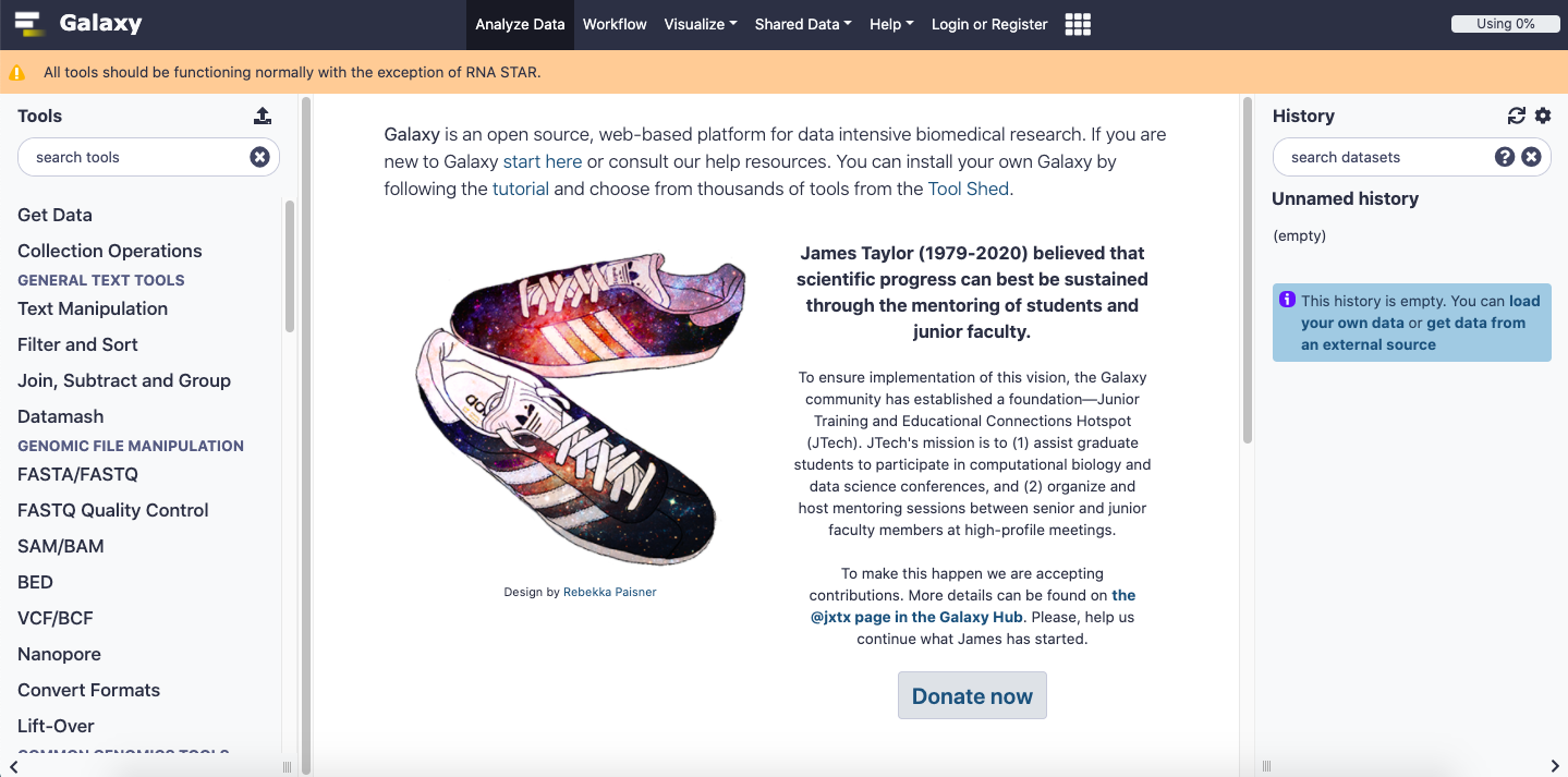
17 |
18 | Hiplot (ORG) (https://hiplot.org) is a free and comprehensive web service for biomedical visualization based on web technology, which is supported by open source communities. It provides more simple web and command-line interfaces compared with other similar platforms.
19 |
20 | Editable table view and switched file uploader simplify the data loading process for most tasks. Data, parameters, and task history can be imported and exported via the JSON files for enhancing reproducibility. A single R language script or function can be used to generate the web front-end interface, command-line interface, and the meta description of a Hiplot plugin. Up to now, hundreds of free applications have been working on Hiplot, including basic statistics, predictive models, multi-omics data analysis, and text-mining.
21 |
22 | This work is licensed under a Creative Commons Attribution 4.0 International License.
23 |
--------------------------------------------------------------------------------
/zh/development-guides/bs4dash.md:
--------------------------------------------------------------------------------
1 | # bs4dash 应用开发指南
2 |
3 | ```r
4 | # load packages
5 | pacman::p_load(shiny)
6 | pacman::p_load(bs4Dash)
7 |
8 |
9 | # ui.R
10 | ## Shiny UI 第一级元素
11 | ?shiny::fluidPage
12 | ?bs4Dash::bs4DashPage
13 |
14 | ## Shiny UI 第二级元素
15 | ?shiny::titlePanel
16 | ?shiny::sidebarLayout
17 | ?shiny::mainPanel
18 | ?bs4Dash::bs4DashNavbar
19 | ?bs4Dash::bs4DashControlbar
20 | ?bs4Dash::bs4DashFooter
21 | ?bs4Dash::bs4DashBody
22 |
23 | ## Shiny UI 第三级元素
24 | ?shiny::sidebarPanel
25 | ?bs4Dash::bs4SidebarMenu
26 | ?bs4Dash::bs4TabItems
27 |
28 | ## Shiny UI 第四级元素
29 | ?bs4Dash::bs4TabItem
30 |
31 | ## Shiny UI 第五级元素
32 | ?bs4Dash::fluidRow
33 |
34 | ## Shiny UI 第六级元素
35 | ?bs4Dash::bs4Box
36 | ?bs4Dash::bs4Accordion
37 | ?bs4Dash::bs4AccordionItem
38 | ?bs4Dash::bs4Alert
39 | ?bs4Dash::bs4Badge
40 | ?bs4Dash::bs4Callout
41 | ?bs4Dash::bs4Card
42 | ?bs4Dash::bs4CardLabel
43 | ?bs4Dash::bs4CardLayout
44 | ?bs4Dash::bs4CardSidebar
45 | ?bs4Dash::bs4Carousel
46 | ?bs4Dash::bs4CarouselItem
47 | ?bs4Dash::bs4CloseAlert
48 | ?bs4Dash::bs4DropdownMenu
49 | ?bs4Dash::bs4DropdownMenuItem
50 | ?bs4Dash::bs4HideTab
51 | ?bs4Dash::bs4InfoBox
52 | ?bs4Dash::bs4InsertTab
53 | ?bs4Dash::bs4Jumbotron
54 | ?bs4Dash::bs4ListGroup
55 | ?bs4Dash::bs4ListGroupItem
56 | ?bs4Dash::bs4Quote
57 | ?bs4Dash::bs4SocialCard
58 | ?bs4Dash::bs4Timeline
59 | ?bs4Dash::bs4Table
60 | ?bs4Dash::bs4Toast
61 | ?bs4Dash::bs4UserCard
62 | ?bs4Dash::bs4ValueBox
63 |
64 | ## Shiny UI 具体展示组件
65 | ?shiny::checkboxGroupInput
66 | ?shiny::checkboxInput
67 | ?shiny::dateInput
68 | ?shiny::dateRangeInput
69 | ?shiny::fileInput
70 | ?shiny::numericInput
71 | ?shiny::passwordInput
72 | ?shiny::restoreInput
73 | ?shiny::selectInput
74 | ?shiny::selectizeInput
75 | ?shiny::sliderInput
76 | ?shiny::snapshotPreprocessInput
77 | ?shiny::textAreaInput
78 | ?shiny::textInput
79 | ?shiny::varSelectInput
80 | ?shiny::varSelectizeInput
81 | ?shiny::downloadButton
82 | ?shiny::downloadLink
83 |
84 | ## Shiny output functions
85 | ?shiny::dataTableOutput
86 | ?shiny::getCurrentOutputInfo
87 | ?shiny::htmlOutput
88 | ?shiny::imageOutput
89 | ?shiny::plotOutput
90 | ?shiny::snapshotPreprocessOutput
91 | ?shiny::tableOutput
92 | ?shiny::textOutput
93 | ?shiny::uiOutput
94 | ?shiny::verbatimTextOutput
95 | ?DT::dataTableOutput
96 | ?DT::DTOutput
97 |
98 | ## bs4Dash是基于Shiny + Bootstrap4扩展而来,
99 | ## 所以Shiny的UI组件可以在library(bs4Dash)后直接使用
100 |
101 | ## 合理使用htmltools包提供的tags下的html标签创建自定义的组件(可CSS语法美化)
102 | ## 如tags$h1("Hello H1",style="font-size:12px;font-weight:bold;color:black;")
103 |
104 | ## 合理使用include
105 | includeCSS() Include Content From a File
106 | includeHTML() Include Content From a File
107 | includeMarkdown() Include Content From a File
108 | includeScript() Include Content From a File
109 | includeText() Include Content From a File
110 | ```
111 |
112 | ```r
113 | # server.R
114 | ?shiny::renderCachedPlot
115 | ?shiny::renderDataTable
116 | ?shiny::renderImage
117 | ?shiny::renderPlot
118 | ?shiny::renderPrint
119 | ?shiny::renderTable
120 | ?shiny::renderText
121 | ?shiny::renderUI
122 | ?DT::renderDT
123 |
124 | # 使用renderUI()可以实现较为强大的功能:
125 | # 1.将数据的列读为新的变量提供给slecteInput()的choice()的参数;
126 | # 2.在Server端设置组件在UI端渲染
127 |
128 | # 合理使用react():
129 | # 1.实现数据动态读取和绘图,同步渲染;
130 | # 2.响应式数据:func <- reactive(data),响应式应用:func()
131 | ```
--------------------------------------------------------------------------------
/qa.md:
--------------------------------------------------------------------------------
1 | # Q&A
2 |
3 | ## Accounts & Contact
4 |
5 | **1. How to contact us?**
6 |
7 | - Send email: admin@hiplot.org;
8 | - Click the feedback button and then send messages;
9 | - Create an issue in https://github.com/hiplot/gold/issues;
10 | - Join the Hiplot [Discord Server](https://discord.gg/vX6tSax) or [Wechat Group](https://docs.qq.com/doc/DS09na3NVYk9OcHVp).
11 |
12 | **2. Do not receive the activation email?**
13 |
14 | - View junk email;
15 | - Change email;
16 | - Contact admin@hiplot.org.
17 |
18 | **3. How to login Hiplot Tiny RSS server?**
19 |
20 | Visit https://hiplot.cn/ttrss, and then use the Hiplot account and the default password 'public'.
21 |
22 | **4. How to login Hiplot Galaxy mirror website?**
23 |
24 | Visit https://galaxy.hiplot.cn, and then use the Hiplot account and the default password 'public'.
25 |
26 | ## Data importing
27 |
28 | **1. Does the data table only show 5000 rows and 99 columns?**
29 |
30 | The actual number of rows and columns behind the data is complete. Both pasted and imported data will be submitted completely, and the data will not be truncated. You can click the export button to confirm.
31 |
32 | **2. After importing the demo data, the scroll bar of the window disappeared?**
33 |
34 | Just move the mouse out of the table.
35 |
36 | **3. Can't copy data from Excel?**
37 |
38 | Before copying and pasting, you need to click the corresponding data table before copy-paste.
39 |
40 | ## Usage of Application
41 |
42 | **1. matrix-bubble do not completely show?**
43 |
44 | Change color palette.
45 |
46 | **2. Error: Insufficient values in manual scale?**
47 |
48 | Change color palette.
49 |
50 | **3. WGCNA tasks do not finish?**
51 |
52 | Hiplot only provides single-thread WGCNA analysis, so large data sets will not be able to complete in a short time. It is recommended to conduct a preliminary screening of genes: such as genes with small mutations, removing non-coding genes, etc. In addition, our code has optimized the analysis parameters as much as possible, but because the steps and algorithms involved in the WGCNA analysis itself are relatively complex, we still recommend that users build the analysis environment locally for the construction of the optimal co-expression network at the publication level, and refer to it. The tutorial on the WGCNA official website is completed step by step. Evaluate the stability of data results by adjusting different parameters, and obtain interpretable results with true biological significance.
53 |
54 | **4. Error: GSEA, Bad format - expect ncols: 2 but found: XX on line?**
55 |
56 | Check the top two lines of the .cls file and delete the two lines tail spaces.
57 |
58 | **5. How to keep the same colors in the chord?**
59 |
60 | Change the color palette and do not use the random option.
61 |
62 | **6. Error: GO/KEGG failed:ERROR [2021-03-12 15:18:33] Error in ans[ypos] <- rep(yes, length.out = len)[ypos]: replacement has length zero?**
63 |
64 | Adjust P Value / Q Value threshold to 1.
65 |
66 | **7. GO/KEGG analysis contain empty gray region?**
67 |
68 | It indicates that do not have significantly enriched terms. You can try to adjust P Value / Q Value threshold to 1.
69 |
70 | **8. How to set custom colors?**
71 |
72 | Change the color palette to 'custom', and then input hexadecimal color, e.g. #000000, in the custom color input field. You need to separate multiple hexadecimal colors by space or comma.
73 |
--------------------------------------------------------------------------------
/usage/advance/README.md:
--------------------------------------------------------------------------------
1 | # Advanced Module
2 |
3 | ## [AGFusion](/advance/agfusion)
4 |
5 | Can be used to visualize the structural pattern of fusion genes at the one-dimensional protein and genome level.
6 |
7 | - Data table (four columns):
8 |
9 | gene5 | 5'gene
10 |
11 | gene3 | 3'gene
12 |
13 | breakpoint5 | 5‘ breakpoint
14 |
15 | breakpoint3 | 3‘ breakpoint
16 |
17 | - Extra parameters
18 |
19 | Reference gene version | Genome version number: hg38 or hg19
20 |
21 | Output WT Gene | Output WT gene structure
22 | ## [Chromsomes-Scatter](/advance/chromsomes-scatter)
23 |
24 | Visualize values at chromosomal level.
25 | ## [ClusterProfiler GO/KEGG](/advance/clusterprofiler-go-kegg)
26 |
27 | Detail see [ClusterProfiler Books](https://hiplot-academic.com/books-static/clusterprofiler-book).
28 |
29 | Note:
30 |
31 | - Both the .rds format file or the species name (e.g. hsa and rno) can input in the `KEGG DB` parameter (Demo 2).
32 | - All data columns will be independently calculated for enrichment analysis.
33 | - The empty gray region represents that not found significant items. It is optional to adjust the P/Q value for including more items.
34 | ## [Cola](/advance/cola)
35 |
36 | - Introduction
37 |
38 | Consensus clustering based on cola framwork.
39 |
40 | ## [DiscoverMutTest](/advance/discover-mut-test)
41 |
42 | Can be used to analysing co-occurrence and mutual exclusivity in cancer genomics data.
43 | ## [DoAbsolute](/advance/doabsolute)
44 |
45 | ABSOLUTE infers multiple models of purity, malignant cell ploidy and absolute somatic copy-numbers from copy ratios data. It determines possible models for absolute copy numbers per cancer cell from a mixed DNA population and gives copy numbers for genomic segments, and if provided mutation data, for mutated alleles.
46 |
47 | More to see:
48 |
49 | -
50 | - [Analyzing ABSOLUTE Data](https://www.genepattern.org/analyzing-absolute-data)
51 | ## [Fusion-Circlize](/advance/fusion-circlize)
52 |
53 | Visualize fusion genes at chromosomal level.
54 | ## [GGtree-MSA](/advance/ggtree-msa)
55 |
56 | Can be used to visualize multiple sequence alignment based on ggplot2.
57 | ## [GGtree-MSA](/advance/ggtree-msa)
58 |
59 | Can be used to tree with multiple sequence alignment.
60 | ## [GISTIC2](/advance/gistic2)
61 |
62 | NOTION: please don't use preprocessing feature when you did not get errors related to overlap segments.
63 |
64 | For the new parameters, they are not belong to GISTIC2 software and designed for preprocessing the input file to avoid problem related to overlap segments:
65 |
66 | - Clean Overlap Segments: enable the preprocessing.
67 | - Min Probe Number for Clean: if preprocessing is enabled, use this value to drop segments with probe number less than this value.## [Ideogram-Heat](/advance/ideogram-heat)
68 |
69 | Visualize values at chromosomal level.
70 | ## [Oncoplot](/advance/oncoplot)
71 |
72 | - Introduction
73 |
74 | Oncoplot can be used to display the landscape of genomic mutations in cancer cohort.## [Pathview](/advance/pathview)
75 |
76 | Calculate the mean expression and fill into the KEGG pathway.
77 | ## [Sigflow](/advance/sigflow)
78 |
79 | Sigflow provides useful mutational signature analysis workflows. It can auto-extract mutational signatures, fit mutation data to all/specified COSMIC reference signatures (SBS/DBS/INDEL).
80 |
81 | There is something you need to know when you use this plugin.
82 |
83 | 1. This plugin is not a complete version, if you want more features, refer to .
84 | 2. `MAF` in `Mode` parameter means `SBS` + `DBS` + `INDEL`.
85 | 3. If you set the `Maximum Signature Number` to `-1`, it will automatically set the maximum signature number based on the mutation type you want to extract signatures.
86 | 4. Option `Number of NMF runs` typically set to 30-50.
--------------------------------------------------------------------------------
/zh/README.md:
--------------------------------------------------------------------------------
1 | # 概览
2 |
3 | [中文版](./) | [English Version](../)
4 |
5 |
6 |
7 | 数据可视化在科研工作中发挥着越来越重要的作用。基于可视化图形,我们可以更好地展示科研数据中的主要特征和规律。以生物医学为例,大多数临床医学学生和初级科研工作者一般需要花费数十天乃至数月的时间去熟悉和掌握常用的数据可视化工具,如 SPSS、Origin 和 Graphpad。之后才有可能去完成部分基础的数据统计分析和可视化。 如果是要专门从事数据分析和建模方向的相关人员则还需额外学习一门甚至数门编程语言(如 MATLAB、R 和 Python )。而要达到能够自由探索数据的水平则还需要额外花费更多时间去深入学习和进阶。
8 |
9 | 近年来,随着各类云计算平台(如生物医学领域的 Galaxy 和 DNAnexus)、相关 IT 软硬件基础设施的发展(如分布式计算、容器技术、软件包管理器、数据分析流程构建框架等),初级科研工作者已经可以相对比较轻松地获取相关数据的上游分析结果。特别是当常规组学数据的上游分析流程趋于稳定和完善,数据上游分析流程的可自定义程度和可变程度已经大大降低。而数据分析下游流程中的可视化和个性化深度解读已经成为当前用户面临的最大挑战:
10 |
11 | 1. 开源用户社区开发的可视化软件或方法大多还没有很好的整合在一个统一的用户接口之下;
12 | 2. 国内缺少活跃的针对科研数据可视化的协作社区,"** 画图群" 成为初级科研用户为数不多的选择;
13 | 3. 国内缺少类似于 Graphpad、MATLAB 核心数据可视化软件和平台,在被美国禁用之后,只能花费额外成本进行流程迁移或重头开始开发;
14 | 4. 国内外开发的一些平台和工具用户体验一般:用户界面不够美观;中英文支持的屈指可数;上手仍然有一定难度;部分平台的文件管理不太方便;用户能够主动参与平台建设的屈指可数;
15 | 5. 相关数据可视化工具仍然相对匮乏,杂志和用户需求旺盛,已发布多年的 Circos 圆圈图可视化,通过封装一些便捷操作就可以发表文章:
16 |
17 | - Rasche H, Hiltemann S. Galactic Circos: User-friendly Circos plots within the Galaxy platform. Gigascience. 2020;9(6):giaa065. doi:10.1093/gigascience/giaa065;
18 | - Marx H, Coon JJ. MS-Helios: a Circos wrapper to visualize multi-omic datasets. BMC Bioinformatics. 2019;20(1):21. Published 2019 Jan 11. doi:10.1186/s12859-018-2564-9; Yu Y, Ouyang Y, Yao W.
19 | - shinyCircos: an R/Shiny application for interactive creation of Circos plot. Bioinformatics. 2018;34(7):1229-1231. doi:10.1093/bioinformatics/btx763)
20 |
21 | 
22 |
23 | Hiplot (ORG) 是由 openbiox 社区于 2019 年 10 月发起,并在新冠疫情爆发后快速发展的一个社区开发项目:致力于建立一个快速迭代、支持中英文环境的科研数据可视化平台和协作社区。
24 |
25 | 目前该平台建设已初具规模,已提供 40 余种基于 R 语言的基础可视化的功能:
26 |
27 | 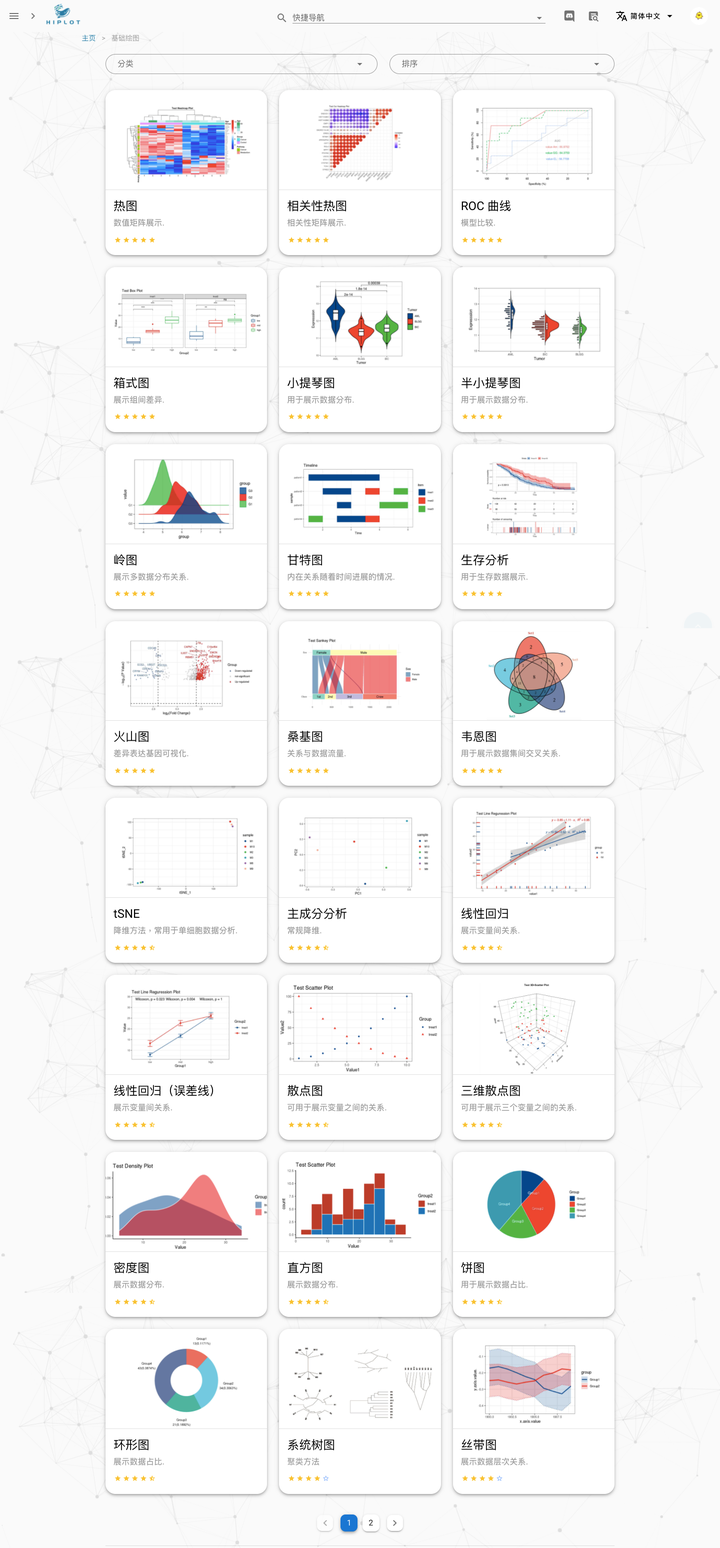
28 |
29 | Hiplot 项目发起的初衷就是为了满足广大临床医学学生和科研工作者科研数据可视化的基础需求:
30 |
31 | 1. 基础可视化:覆盖大多数基础的科研可视化功能,参照 SPSS、GraphPad、国内外开发的相关可视化软件和工具
32 | 2. 进阶可视化:包括 Shiny 在内的复杂可视化图形和应用;文献图表的重现和再分析;新的可视化图形展示插件:如基于 Circos、circlize 的二次开发;openbiox 社区贡献的可视化应用(如 UCSCXenaShiny 和 bioshiny)
33 | 3. 附加模块:低计算量的附加模块(如文献数据资源下载、ID 转换、文件格式转换、RESTful APIs 访问等)
34 | 4. 文件管理(支持上传、下载、复制、移动、删除、在线预览和编辑等操作)
35 |
36 | 其他一些我正在收集和考虑纳入 Hiplot 平台中的可视化功能:
37 |
38 | 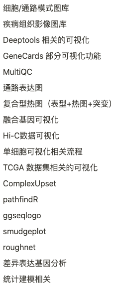
39 |
40 | **用户交互界面展示(部分):**
41 |
42 | 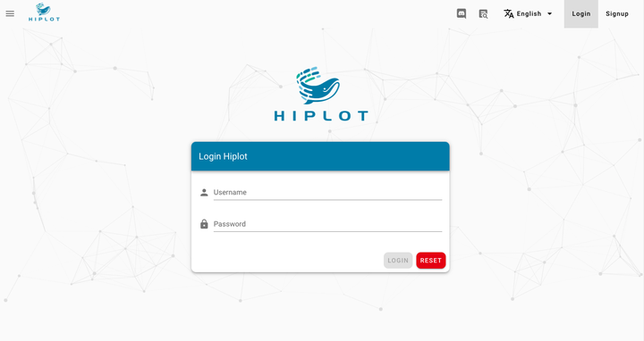
43 |
44 | 登录
45 |
46 | 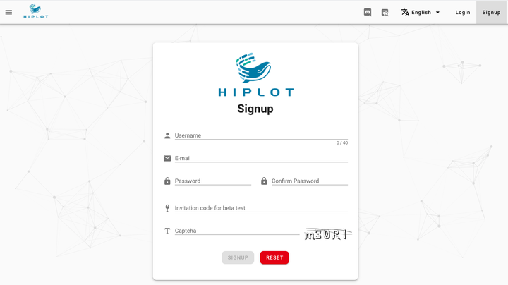
47 |
48 | 注册
49 |
50 | 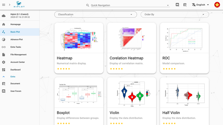
51 |
52 | 基础绘图卡片浏览与检索
53 |
54 | 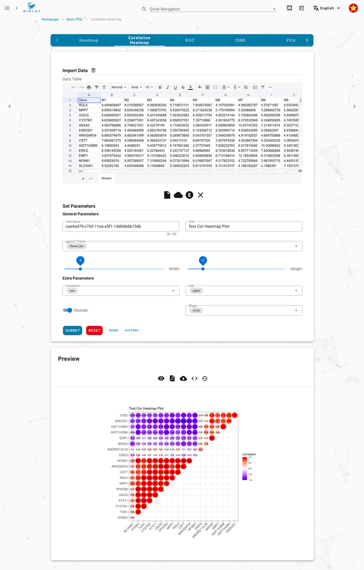
55 |
56 | 绘图示例 | 相关性热图
57 |
58 | 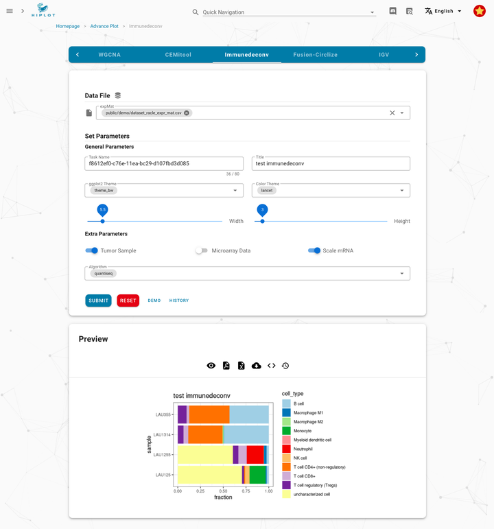
59 |
60 | 绘图示例 | 免疫浸润分析
61 |
62 | 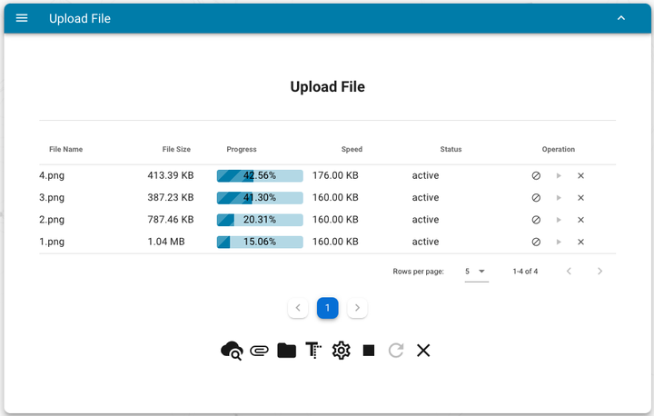
63 |
64 | 文件上传窗口
65 |
66 | 
67 |
68 | 文件浏览与管理
69 |
70 | 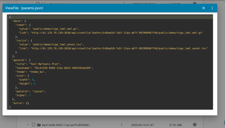
71 |
72 | 文件在线查看和编辑(支持文本文件、XLSX、CSV、TXT 等)
73 |
74 | 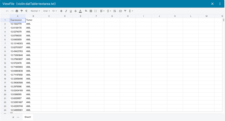
75 |
76 | 文件在线查看和编辑(支持文本文件、XLSX、CSV、TXT 等)
77 |
78 | 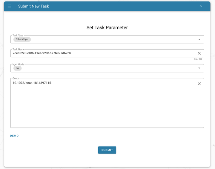
79 |
80 | 提交文献原文和附录下载任务(基于 openbiox 社区贡献的 [bget](https://github.com/openanno/bget) 项目)
81 |
82 | 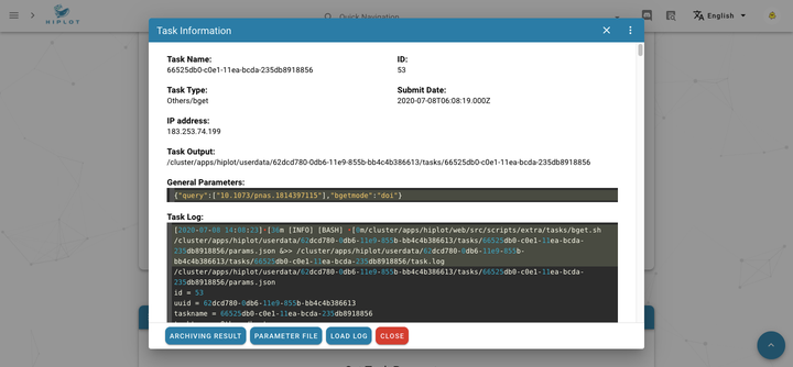
83 |
84 | 提交文献原文和附录下载任务(基于 openbiox 社区贡献的 [bget](https://github.com/openanno/bget) 项目)
85 |
86 | 如果你想贡献 Hiplot 项目,欢迎加入我们的用户社区:[Discord](https://discord.gg/vX6tSax)
87 |
88 | 本文档内容遵循 Creative Commons Attribution 4.0 International License.
89 |
--------------------------------------------------------------------------------
/env.Rmd:
--------------------------------------------------------------------------------
1 | # Cloud environment
2 |
3 | ```{r setup, include=FALSE}
4 | knitr::opts_chunk$set(echo = TRUE)
5 | ```
6 | ## Basic Info
7 |
8 | ```{r message=FALSE, warning=FALSE, echo=FALSE}
9 | pacman::p_load(RMySQL)
10 | pacman::p_load(configr)
11 | conf_raw <- read.config('../conf/config.json')
12 | #conf <- conf_raw$mysql
13 | #conn <- dbConnect(MySQL(), dbname = conf$database, username=conf$username,
14 | # password=conf$password, host=conf$host, port=conf$port)
15 | #raw <- dbReadTable(conn, "users")
16 |
17 | json <- system('cd ../conf/baidu; sh fetch.sh pv', intern = TRUE)
18 | json <- configr::str2config(paste0(json, '\n'))
19 | json <- as.data.frame(json$body$data$result$items[[1]][2])
20 | total_pv <- suppressWarnings(sum(as.numeric(json[,1]), na.rm = T))
21 | total_visitor <- suppressWarnings(sum(as.numeric(json[,2]), na.rm = T))
22 |
23 | Term <- c('Hiplot Version', "Total (PV)", "Total (UV)", 'Update Date')
24 | Value <- c(conf_raw$version, total_pv, total_visitor, as.character( Sys.time()))
25 | dat <- data.frame(Term, Value)
26 | x <- write.config(as.list(dat), "/app/hiplot/dist/docs/pv.json", write.type = "json")
27 | knitr::kable(dat, row.names = F)
28 | ```
29 |
30 | ## System Info
31 |
32 | ```{r message=FALSE, warning=FALSE, echo=FALSE}
33 | dat <- as.data.frame(data.table::fread("cat /proc/cpuinfo", fill=T, sep = '\t'))
34 | dat <- dat[,c(1,3)]
35 | dat[,2] <- stringr::str_replace(dat[,2], ' :|:', '')
36 | dat <- dat[!duplicated(dat[,1]),]
37 | colnames(dat) <- c('Term', 'Info')
38 | total_logical_num <- system("cat /proc/cpuinfo| grep 'processor'| wc -l", intern = TRUE)
39 | physical_num <- system("cat /proc/cpuinfo| grep 'physical id'| sort| uniq| wc -l", intern = TRUE)
40 | core_num_per <- system("cat /proc/cpuinfo| grep 'cpu cores'| uniq | sed 's/.* //'", intern = TRUE)
41 | loadavg <- data.table::fread("cat /proc/loadavg", data.table = FALSE)
42 | tmp <- data.frame(Term=c("Linux Kernel", "Total Logical Cores", "Physical CPU", "Cores Per CPU", "Load Avg"),
43 | Info=c(system('uname -s -r', intern = TRUE), total_logical_num, physical_num, core_num_per, loadavg[1, 4]))
44 | dat <- rbind(tmp, dat)
45 | dat_cpu <- dat[dat[,2] != '',]
46 | Tag <- rep('cpu', nrow(dat_cpu))
47 | Tag[1] <- 'linux'
48 | dat_cpu <- cbind(dat_cpu, Tag)
49 |
50 | dat <- as.data.frame(data.table::fread('cat /proc/meminfo', fill = TRUE))
51 | dat <- dat[,1:2]
52 | use_kb <- dat[,2] < 1024
53 | use_mb <- dat[,2] >= 1024
54 | use_gb <- dat[,2] >= 1024 * 1024
55 | use_tb <- dat[,2] >= 1024 * 1024 * 1024
56 | use_pb <- dat[,2] >= 1024 * 1024 * 1024 * 1024
57 | dat$Size <- NA
58 |
59 | if (sum(use_kb) > 0) {
60 | dat[use_kb,3] <- paste0(dat[use_kb,2], ' KB')
61 | }
62 | if (sum(use_mb) > 0) {
63 | dat[use_mb,3] <- paste0(round(dat[use_mb,2] / 1024, 2), ' MB')
64 | }
65 |
66 | if (sum(use_gb) > 0) {
67 | dat[use_gb,3] <- paste0(round(dat[use_gb,2] / (1024 * 1024), 2), ' GB')
68 | }
69 | if (sum(use_tb) > 0) {
70 | dat[use_tb,3] <- paste0(round(dat[use_tb,2] / (1024 * 1024 * 1024), 2), ' TB')
71 | }
72 | if (sum(use_pb) > 0) {
73 | dat[use_pb,3] <- paste0(round(dat[use_pb,2] / (1024 * 1024 * 1024 * 1024), 2), ' PB')
74 | }
75 | dat <- dat[,-2]
76 | colnames(dat) <- c('Term', "Info")
77 | Tag <- rep('mem', nrow(dat))
78 | dat_mem <- cbind(dat, Tag)
79 |
80 | dat <- data.table::fread("df -h /| sed 's/ */\t/g' | cut -f 2,3,4,5")
81 | dat_disk <- as.data.frame(t(dat))
82 | dat_disk <- cbind(row.names(dat_disk), dat_disk)
83 | dat_disk[,1] <- paste0('DISK ', dat_disk[,1])
84 | dat_disk$Tag <- "disk"
85 | colnames(dat_disk)[1:2] <- c('Term', "Info")
86 | dat <- rbind(dat_cpu, dat_mem, dat_disk)
87 | dat[,1] <- Hmisc::capitalize(dat[,1])
88 | x <- write.config(as.list(dat), "/app/hiplot/dist/docs/hardware.json", write.type = "json")
89 | knitr::kable(dat, row.names = F)
90 | ```
91 |
92 | ## Installed RPM packages
93 |
94 | ```{r message=FALSE, warning=FALSE, echo=FALSE}
95 | dat <- read.csv('data/yum_installed_pkgs.txt', sep = '\t')
96 | knitr::kable(dat, row.names = F)
97 | ```
98 |
99 | ## Installed R Packages
100 |
101 | ```{r message=FALSE, warning=FALSE, echo=FALSE}
102 | dat <- installed.packages()[,c(1,3, 10, 16)]
103 | knitr::kable(dat, row.names = F)
104 | ```
105 |
106 | ## Installed Python packages
107 |
108 | ```{r message=FALSE, warning=FALSE, echo=FALSE}
109 | dat <- BioInstaller::conda.list()
110 | knitr::kable(dat, row.names = F)
111 | ```
112 |
113 | ## Sessioninfo
114 |
115 | ```{r message=FALSE, warning=FALSE, echo=FALSE}
116 | sessioninfo::session_info()
117 | ```
118 |
119 |
--------------------------------------------------------------------------------
/.vuepress/config.js:
--------------------------------------------------------------------------------
1 | module.exports = {
2 | temp: '/tmp/vuepress.temp',
3 | base: '/docs/',
4 | host: '0.0.0.0',
5 | head: [
6 | // 添加百度统计
7 | [
8 | "script",
9 | {},
10 | `
11 | var _hmt = _hmt || [];
12 | (function () {
13 | var hm = document.createElement("script");
14 | hm.src = "https://hm.baidu.com/hm.js?0b834e1080e98dd6144a263303f8bd1b";
15 | var s = document.getElementsByTagName("script")[0];
16 | s.parentNode.insertBefore(hm, s);
17 | })();
18 | `
19 | ]
20 | ],
21 | locales: {
22 | // 键名是该语言所属的子路径
23 | // 作为特例,默认语言可以使用 '/' 作为其路径。
24 | '/': {
25 | lang: 'en-US', // 将会被设置为 的 lang 属性
26 | "title": 'Hiplot',
27 | description: 'Visualization'
28 | },
29 | '/zh/': {
30 | lang: 'zh-CN',
31 | "title": 'Hiplot',
32 | description: '可视化'
33 | }
34 | },
35 | themeConfig: {
36 | locales: {
37 | // 键名是该语言所属的子路径
38 | // 作为特例,默认语言可以使用 '/' 作为其路径。
39 | '/': {
40 | selectText: 'Languages',
41 | label: 'English',
42 | editLinkText: 'Edit this page on GitHub',
43 | serviceWorker: {
44 | updatePopup: {
45 | message: "New content is available.",
46 | buttonText: "Refresh"
47 | }
48 | },
49 | nav: [
50 | { text: 'Home', link: 'https://hiplot.cn' },
51 | { text: 'Docs', link: '/' },
52 | { text: 'Community', link: 'https://discord.com/channels/708004190286381068' },
53 | ],
54 | algolia: {},
55 | sidebar: [
56 | {
57 | "title": 'Introduction',
58 | collapsable: true,
59 | children: [
60 | '/',
61 | '/modules',
62 | '/env',
63 | '/download/',
64 | '/qa',
65 | '/contribute',
66 | '/about'
67 | ]
68 | },
69 | {
70 | "title": 'Getting Started',
71 | collapsable: true,
72 | children: [
73 | '/usage/basic/',
74 | '/usage/advance/',
75 | '/usage/mini-tools/',
76 | '/usage/clinical-tools/'
77 | ]
78 | },
79 | {
80 | "title": 'Development Guidance',
81 | collapsable: true,
82 | children: [
83 | '/development-guides/',
84 | '/development-guides/hisub'
85 | ]
86 | }
87 | ],
88 | },
89 | '/zh/': {
90 | selectText: '选择语言',
91 | // 该语言在下拉菜单中的标签
92 | label: '简体中文',
93 | // 编辑链接文字
94 | editLinkText: '在 GitHub 上编辑此页',
95 | // Service Worker 的配置
96 | serviceWorker: {
97 | updatePopup: {
98 | message: "发现新内容可用.",
99 | buttonText: "刷新"
100 | }
101 | },
102 | nav: [
103 | { text: '主页', link: 'https://hiplot.cn' },
104 | { text: '文档', link: '/zh/' },
105 | { text: '用户社区', link: 'https://discord.com/channels/708004190286381068' },
106 | ],
107 | // 当前 locale 的 algolia docsearch 选项
108 | algolia: {},
109 | sidebar: [
110 | {
111 | "title": '简介',
112 | collapsable: true,
113 | children: [
114 | '/zh/',
115 | '/zh/modules',
116 | '/zh/hisub',
117 | '/zh/download/'
118 | ]
119 | },
120 | {
121 | "title": '入门指南',
122 | collapsable: true,
123 | children: [
124 | '/zh/usage/basic/',
125 | '/zh/usage/advance/',
126 | '/zh/usage/mini-tools/',
127 | '/zh/usage/clinical-tools/'
128 | ]
129 | },
130 | {
131 | "title": '开发指南',
132 | collapsable: true,
133 | children: [
134 | '/zh/development-guides/',
135 | '/zh/development-guides/bs4dash',
136 | '/zh/development-guides/run'
137 | ]
138 | }
139 | ],
140 | }
141 | },
142 |
143 | sidebarDepth: 2,
144 | activeHeaderLinks: false,
145 | displayAllHeaders: true,
146 | repo: 'hiplot/docs',
147 |
148 | lastUpdated: 'Last Updated',
149 | },
150 | configureWebpack: {
151 | resolve: {
152 | alias: {
153 | '@': '../'
154 | }
155 | }
156 | }
157 | }
158 |
--------------------------------------------------------------------------------
/zh/download/README.md:
--------------------------------------------------------------------------------
1 | # Download
2 |
3 |
4 |
5 | ## 桌面客户端
6 |
7 | 我们基于 [Electron](https://www.electronjs.org/) 构建了 Hiplot 的桌面客户端。示例数据和 UI 组件将在特定版本下被固定。
8 |
9 | 最新版本:
10 |
11 |
12 | |File |Size |Date |MD5 |
13 | |:-------------------------------------|:--------|:----------|:--------------------------------|
14 | |[Hiplot_Desktop_0.2.0_Darwin.dmg](https://download.hiplot.cn/download/desktop/v0.2.0/Hiplot_Desktop_0.2.0_Darwin.dmg)|85.5 Mb |2022-04-23 |3b9b172ad7c42f21cc5cad7193d3e6fa |
15 | |[Hiplot_Desktop_0.2.0_Linux_amd64.deb](https://download.hiplot.cn/download/desktop/v0.2.0/Hiplot_Desktop_0.2.0_Linux_amd64.deb)|59.8 Mb |2022-04-23 |1364a9cdda29899cdf7559b21c795839 |
16 | |[Hiplot_Desktop_0.2.0_Linux_x64.apk](https://download.hiplot.cn/download/desktop/v0.2.0/Hiplot_Desktop_0.2.0_Linux_x64.apk)|87.2 Mb |2022-04-23 |1da132999464e6d8cec6d5bf28f33912 |
17 | |[Hiplot_Desktop_0.2.0_Linux_x86_64.rpm](https://download.hiplot.cn/download/desktop/v0.2.0/Hiplot_Desktop_0.2.0_Linux_x86_64.rpm)|59.9 Mb |2022-04-23 |1cbaf4cbe039a68cf3c6abeeabacf861 |
18 | |[Hiplot_Desktop_0.2.0_Windows.exe](https://download.hiplot.cn/download/desktop/v0.2.0/Hiplot_Desktop_0.2.0_Windows.exe)|127.7 Mb |2022-04-23 |e3209b49148a2107ef4cc5f28de48558 |
19 | |[Hiplot_Desktop_0.2.0_Windows_ia32.exe](https://download.hiplot.cn/download/desktop/v0.2.0/Hiplot_Desktop_0.2.0_Windows_ia32.exe)|62.7 Mb |2022-04-23 |bc70b084a6e7357ba2514b053c74ffc8 |
20 | |[Hiplot_Desktop_0.2.0_Windows_x64.exe](https://download.hiplot.cn/download/desktop/v0.2.0/Hiplot_Desktop_0.2.0_Windows_x64.exe)|65.8 Mb |2022-04-23 |9e52e69fe0089ac2d9f411a91e29c0ac |
21 |
22 | 其他桌面版本: [这里](https://download.hiplot.cn/download/desktop/)
23 |
24 | ## hctl
25 |
26 | hctl 是 Hiplot 网站的命令行程序. 它可以让用户在命令行环境下使用 Hiplot 网站的绘图系统。
27 |
28 | 最新发布版本 (v0.1.7):
29 |
30 |
31 | |File |Size |Date |MD5 |
32 | |:--------------------------------|:------|:----------|:--------------------------------|
33 | |[hctl_0.1.7_Darwin_64-bit.tar.gz](https://download.hiplot.cn/download/hctl/v0.1.7/hctl_0.1.7_Darwin_64-bit.tar.gz)|3 Mb |2023-02-08 |19173d8631683c3bd751310c38fbb65c |
34 | |[hctl_0.1.7_Darwin_arm64.tar.gz](https://download.hiplot.cn/download/hctl/v0.1.7/hctl_0.1.7_Darwin_arm64.tar.gz)|2.9 Mb |2023-02-08 |e19f342414414c7c9597e94a8ed60207 |
35 | |[hctl_0.1.7_Linux_32-bit.tar.gz](https://download.hiplot.cn/download/hctl/v0.1.7/hctl_0.1.7_Linux_32-bit.tar.gz)|2.8 Mb |2023-02-08 |7d032a64356320f71f817de0fc8219b4 |
36 | |[hctl_0.1.7_Linux_64-bit.tar.gz](https://download.hiplot.cn/download/hctl/v0.1.7/hctl_0.1.7_Linux_64-bit.tar.gz)|2.9 Mb |2023-02-08 |cfc2c81bbe3486e4fbc75ae80ee71d6f |
37 | |[hctl_0.1.7_Linux_arm64.tar.gz](https://download.hiplot.cn/download/hctl/v0.1.7/hctl_0.1.7_Linux_arm64.tar.gz)|2.7 Mb |2023-02-08 |e61edbf465586c832d9b0bd7827ec9a7 |
38 | |[hctl_0.1.7_Windows_32-bit.tar.gz](https://download.hiplot.cn/download/hctl/v0.1.7/hctl_0.1.7_Windows_32-bit.tar.gz)|2.9 Mb |2023-02-08 |21a1ee95e7f6cf48f029396fb2d5dc77 |
39 | |[hctl_0.1.7_Windows_64-bit.tar.gz](https://download.hiplot.cn/download/hctl/v0.1.7/hctl_0.1.7_Windows_64-bit.tar.gz)|2.9 Mb |2023-02-08 |082bfe11a98b9458fa0c3021e3b1ca67 |
40 | |[hctl_0.1.7_Windows_arm64.tar.gz](https://download.hiplot.cn/download/hctl/v0.1.7/hctl_0.1.7_Windows_arm64.tar.gz)|2.7 Mb |2023-02-08 |3e6adef0e76a799eb15add028d26ae66 |
41 |
42 | 其他 hctl 版本: [这里](https://hiplot.cn/download/hctl)
43 |
44 | 使用 hctl 进行绘图之前,用户需要使用 `hctl login` 命令获得 Hiplot 的服务授权。 登录成功后,即可使用 `hctl plot` 命令进行绘图:输入数据为一个 JSON 格式的参数文件和/或一个/多个数据表。
45 |
46 | 示例输入 [demo.tar.gz](https://hiplot.cn/download/hctl/_demo.tar.gz)。
47 |
48 | ```bash
49 | ## Linux 64 Demo
50 | mkdir /tmp/hiplot
51 | cd /tmp/hiplot
52 | wget https://hiplot.cn/download/hctl/v0.1.7/hctl_0.1.7_Linux_64-bit.tar.gz
53 | wget https://hiplot.cn/download/hctl/_demo.tar.gz
54 |
55 | tar -xzvf hctl_0.1.7_Linux_64-bit.tar.gz
56 | tar -xzvf _demo.tar.gz
57 |
58 | ./hctl login
59 |
60 | # 只输入本地数据文件
61 | ./hctl plot -c _demo/heatmap/config.json -t heatmap -d _demo/heatmap/countData.txt,_demo/heatmap/sampleInfo.txt,_demo/heatmap/geneInfo.txt -o /tmp/hiplot-pure-data-mode
62 |
63 | # 只使用远程服务器文件
64 | ./hctl plot -c _demo/heatmap/config2.json -t heatmap -o /tmp/hiplot-pure-remote-data-mode
65 |
66 | # 混合使用本地数据和远程服务器文件
67 | ./hctl plot -c _demo/heatmap/config3.json -t heatmap -d _demo/heatmap/countData.txt,,_demo/heatmap/geneInfo.txt -o /tmp/hiplot-mixed-mode
68 |
69 | # 使用 Hiplot 网站导出的参数文件
70 | ./hctl plot -p _demo/heatmap/params.json -t heatmap -o /tmp/hiplot-params-mode
71 |
72 | # hiplot config 和 plot 命令联合
73 | ## 展示 hctl 支持的网页插件
74 | hctl config -l
75 | ## 下载 basic/tsne 插件配置文件
76 | hctl config basic/tsne
77 | ## 绘制 tsne 图形
78 | hctl plot -p basic-tsne-params.json -o /tmp/hiplot-tsne
79 | ```
80 |
81 | ### 命令行主程序
82 |
83 |
84 | ```
85 | ## Command-line client to draw plots of [Hiplot](https://hiplot.cn) website. More see here https://github.com/hiplot.
86 | ##
87 | ## Usage:
88 | ## hctl [flags]
89 | ## hctl [command]
90 | ##
91 | ## Available Commands:
92 | ## completion Generate the autocompletion script for the specified shell
93 | ## config Initializing a config.json file of hiplot application.
94 | ## help Help about any command
95 | ## login Login Hiplot Website.
96 | ## plot Plot functions of Hiplot Website.
97 | ##
98 | ## Flags:
99 | ## -h, --help help for hctl
100 | ## --log-dir string log dir. (default "/tmp/_log")
101 | ## -o, --out-dir string output dir. (default "/tmp")
102 | ## --proxy string HTTP proxy to query.
103 | ## --save-log Save log to file.
104 | ## -k, --taskname string task ID (default is random). (default "db1cfb4f-c323-4da7-9a45-a09b135d7430")
105 | ## --timeout int set the timeout of per request. (default 35)
106 | ## --verbose int verbose level (0:no output, 1: basic level, 2: with env info) (default 1)
107 | ## -v, --version version for hctl
108 | ##
109 | ## Use "hctl [command] --help" for more information about a command.
110 | ```
111 |
112 | ### 绘图子程序
113 |
114 |
115 | ```
116 | ## Plot functions of Hiplot Website.
117 | ##
118 | ## Usage:
119 | ## hctl plot [flags]
120 | ##
121 | ## Examples:
122 | ## hctl plot -c _demo/heatmap/config.json -t heatmap -d _demo/heatmap/countData.txt,_demo/heatmap/sampleInfo.txt,_demo/heatmap/geneInfo.txt -o /tmp/hiplot-pure-data-mode
123 | ## hctl plot -c _demo/heatmap/config2.json -t heatmap -o /tmp/hiplot-pure-remote-data-mode
124 | ## hctl plot -c _demo/heatmap/config3.json -t heatmap -d _demo/heatmap/countData.txt,,_demo/heatmap/geneInfo.txt -o /tmp/hiplot-mixed-mode
125 | ## hctl plot -p _demo/heatmap/params.json -t heatmap -o /tmp/hiplot-params-mode
126 | ## hctl plot -p _demo/heatmap/params2.json -o /tmp/hiplot-params-mode2
127 | ## hctl plot -p _demo/heatmap/basic-heatmap-params.json --load-example true -o /tmp/hiplot-params-mode3
128 | ## hctl plot --check-task --temp-code QwbMBp7 --taskname 62919a54-ee68-49c4-b070-7384c60fb05f --tool clusterprofiler-go-kegg -m advance -o /tmp/clusterprofiler-go-kegg
129 | ## hctl config basic/pca
130 | ## hctl plot -p basic-pca-params.json --load-example true -o /tmp/pca1
131 | ## hctl plot -p basic-pca-params.json --load-example 2 -o /tmp/pca2
132 | ## hctl plot -p _demo/tsne/basic-tsne-params.json -o /tmp/hiplot-tsne --load-example true
133 | ##
134 | ## Flags:
135 | ## --check-task check task status, taskname and tmpcode are required.
136 | ## -c, --config string json format tool config file.
137 | ## -d, --data string data table file (sepreate by comma).
138 | ## -h, --help help for plot
139 | ## --load-example string load example field (only work for hctl config export) (default "false")
140 | ## -m, --module string module name: basic, advance. (default "basic")
141 | ## -p, --params string json format tool params file (exported by Hiplot).
142 | ## --print-links print result links
143 | ## --temp-code string task tempcode. (default "2rSx7qr")
144 | ## -t, --tool string tool name (e.g. heatmap).
145 | ##
146 | ## Global Flags:
147 | ## --log-dir string log dir. (default "/tmp/_log")
148 | ## -o, --out-dir string output dir. (default "/tmp")
149 | ## --proxy string HTTP proxy to query.
150 | ## --save-log Save log to file.
151 | ## -k, --taskname string task ID (default is random). (default "e4b4114f-83ad-4de8-aac6-19741ac82fe7")
152 | ## --timeout int set the timeout of per request. (default 35)
153 | ## --verbose int verbose level (0:no output, 1: basic level, 2: with env info) (default 1)
154 | ```
155 |
--------------------------------------------------------------------------------
/download/README.md:
--------------------------------------------------------------------------------
1 | # Download
2 |
3 |
4 |
5 | ## Desktop Client
6 |
7 | We build the desktop client of Hiplot (ORG) based on the [Electron](https://www.electronjs.org/). The demo data and UI components are fixed in the desktop client under the given version.
8 |
9 | Latest release version:
10 |
11 |
12 | |File |Size |Date |MD5 |
13 | |:-------------------------------------|:--------|:----------|:--------------------------------|
14 | |[Hiplot_Desktop_0.2.0_Darwin.dmg](https://download.hiplot.cn/download/desktop/v0.2.0/Hiplot_Desktop_0.2.0_Darwin.dmg)|85.5 Mb |2022-04-23 |3b9b172ad7c42f21cc5cad7193d3e6fa |
15 | |[Hiplot_Desktop_0.2.0_Linux_amd64.deb](https://download.hiplot.cn/download/desktop/v0.2.0/Hiplot_Desktop_0.2.0_Linux_amd64.deb)|59.8 Mb |2022-04-23 |1364a9cdda29899cdf7559b21c795839 |
16 | |[Hiplot_Desktop_0.2.0_Linux_x64.apk](https://download.hiplot.cn/download/desktop/v0.2.0/Hiplot_Desktop_0.2.0_Linux_x64.apk)|87.2 Mb |2022-04-23 |1da132999464e6d8cec6d5bf28f33912 |
17 | |[Hiplot_Desktop_0.2.0_Linux_x86_64.rpm](https://download.hiplot.cn/download/desktop/v0.2.0/Hiplot_Desktop_0.2.0_Linux_x86_64.rpm)|59.9 Mb |2022-04-23 |1cbaf4cbe039a68cf3c6abeeabacf861 |
18 | |[Hiplot_Desktop_0.2.0_Windows.exe](https://download.hiplot.cn/download/desktop/v0.2.0/Hiplot_Desktop_0.2.0_Windows.exe)|127.7 Mb |2022-04-23 |e3209b49148a2107ef4cc5f28de48558 |
19 | |[Hiplot_Desktop_0.2.0_Windows_ia32.exe](https://download.hiplot.cn/download/desktop/v0.2.0/Hiplot_Desktop_0.2.0_Windows_ia32.exe)|62.7 Mb |2022-04-23 |bc70b084a6e7357ba2514b053c74ffc8 |
20 | |[Hiplot_Desktop_0.2.0_Windows_x64.exe](https://download.hiplot.cn/download/desktop/v0.2.0/Hiplot_Desktop_0.2.0_Windows_x64.exe)|65.8 Mb |2022-04-23 |9e52e69fe0089ac2d9f411a91e29c0ac |
21 |
22 | Other releases of desktop client: [here](https://hiplot.cn/download/desktop)
23 |
24 | ## hctl
25 |
26 | hctl is the command-line client of Hiplot (ORG) website. It can be used to draw plots without the web environment.
27 |
28 | Latest release version (v0.1.7):
29 |
30 |
31 | |File |Size |Date |MD5 |
32 | |:--------------------------------|:------|:----------|:--------------------------------|
33 | |[hctl_0.1.7_Darwin_64-bit.tar.gz](https://download.hiplot.cn/download/hctl/v0.1.7/hctl_0.1.7_Darwin_64-bit.tar.gz)|3 Mb |2023-02-08 |19173d8631683c3bd751310c38fbb65c |
34 | |[hctl_0.1.7_Darwin_arm64.tar.gz](https://download.hiplot.cn/download/hctl/v0.1.7/hctl_0.1.7_Darwin_arm64.tar.gz)|2.9 Mb |2023-02-08 |e19f342414414c7c9597e94a8ed60207 |
35 | |[hctl_0.1.7_Linux_32-bit.tar.gz](https://download.hiplot.cn/download/hctl/v0.1.7/hctl_0.1.7_Linux_32-bit.tar.gz)|2.8 Mb |2023-02-08 |7d032a64356320f71f817de0fc8219b4 |
36 | |[hctl_0.1.7_Linux_64-bit.tar.gz](https://download.hiplot.cn/download/hctl/v0.1.7/hctl_0.1.7_Linux_64-bit.tar.gz)|2.9 Mb |2023-02-08 |cfc2c81bbe3486e4fbc75ae80ee71d6f |
37 | |[hctl_0.1.7_Linux_arm64.tar.gz](https://download.hiplot.cn/download/hctl/v0.1.7/hctl_0.1.7_Linux_arm64.tar.gz)|2.7 Mb |2023-02-08 |e61edbf465586c832d9b0bd7827ec9a7 |
38 | |[hctl_0.1.7_Windows_32-bit.tar.gz](https://download.hiplot.cn/download/hctl/v0.1.7/hctl_0.1.7_Windows_32-bit.tar.gz)|2.9 Mb |2023-02-08 |21a1ee95e7f6cf48f029396fb2d5dc77 |
39 | |[hctl_0.1.7_Windows_64-bit.tar.gz](https://download.hiplot.cn/download/hctl/v0.1.7/hctl_0.1.7_Windows_64-bit.tar.gz)|2.9 Mb |2023-02-08 |082bfe11a98b9458fa0c3021e3b1ca67 |
40 | |[hctl_0.1.7_Windows_arm64.tar.gz](https://download.hiplot.cn/download/hctl/v0.1.7/hctl_0.1.7_Windows_arm64.tar.gz)|2.7 Mb |2023-02-08 |3e6adef0e76a799eb15add028d26ae66 |
41 |
42 | Other releases of hctl: [here](https://hiplot.cn/download/hctl)
43 |
44 | It is required to login Hiplot (ORG) server first using the `hctl login` command. `hctl plot` command can be used to draw plots by using the parameter file and data files.
45 |
46 | Demo input files of hctl can be download from here: [demo.tar.gz](https://hiplot.cn/download/hctl/_demo.tar.gz).
47 |
48 | ```bash
49 | ## Linux 64 Demo
50 | mkdir /tmp/hiplot
51 | cd /tmp/hiplot
52 | wget https://hiplot.cn/download/hctl/v0.1.7/hctl_0.1.7_Linux_64-bit.tar.gz
53 | wget https://hiplot.cn/download/hctl/_demo.tar.gz
54 |
55 | tar -xzvf hctl_0.1.7_Linux_64-bit.tar.gz
56 | tar -xzvf _demo.tar.gz
57 |
58 | hctl login
59 |
60 | # only input data files
61 | hctl plot -c _demo/heatmap/config.json -t heatmap -d _demo/heatmap/countData.txt,_demo/heatmap/sampleInfo.txt,_demo/heatmap/geneInfo.txt -o /tmp/hiplot-pure-data-mode
62 |
63 | # only use remote files
64 | hctl plot -c _demo/heatmap/config2.json -t heatmap -o /tmp/hiplot-pure-remote-data-mode
65 |
66 | # mixed usage
67 | hctl plot -c _demo/heatmap/config3.json -t heatmap -d _demo/heatmap/countData.txt,,_demo/heatmap/geneInfo.txt -o /tmp/hiplot-mixed-mode
68 |
69 | # hiplot exported params
70 | hctl plot -p _demo/heatmap/params.json -t heatmap -o /tmp/hiplot-params-mode
71 |
72 | # hiplot config 和 plot 命令联合
73 | ## show hctl supported plugins
74 | hctl config -l
75 | ## download basic/tsne params
76 | hctl config basic/tsne
77 | ## draw tsne graphics
78 | hctl plot -p basic-tsne-params.json -o /tmp/hiplot-tsne
79 | ```
80 |
81 | ### Main Interface
82 |
83 |
84 | ```
85 | ## Command-line client to draw plots of [Hiplot](https://hiplot.cn) website. More see here https://github.com/hiplot.
86 | ##
87 | ## Usage:
88 | ## hctl [flags]
89 | ## hctl [command]
90 | ##
91 | ## Available Commands:
92 | ## completion Generate the autocompletion script for the specified shell
93 | ## config Initializing a config.json file of hiplot application.
94 | ## help Help about any command
95 | ## login Login Hiplot Website.
96 | ## plot Plot functions of Hiplot Website.
97 | ##
98 | ## Flags:
99 | ## -h, --help help for hctl
100 | ## --log-dir string log dir. (default "/tmp/_log")
101 | ## -o, --out-dir string output dir. (default "/tmp")
102 | ## --proxy string HTTP proxy to query.
103 | ## --save-log Save log to file.
104 | ## -k, --taskname string task ID (default is random). (default "435f5f32-4750-4e74-b97e-13a40d5d0f3e")
105 | ## --timeout int set the timeout of per request. (default 35)
106 | ## --verbose int verbose level (0:no output, 1: basic level, 2: with env info) (default 1)
107 | ## -v, --version version for hctl
108 | ##
109 | ## Use "hctl [command] --help" for more information about a command.
110 | ```
111 |
112 | ### Plot Interface
113 |
114 |
115 | ```
116 | ## Plot functions of Hiplot Website.
117 | ##
118 | ## Usage:
119 | ## hctl plot [flags]
120 | ##
121 | ## Examples:
122 | ## hctl plot -c _demo/heatmap/config.json -t heatmap -d _demo/heatmap/countData.txt,_demo/heatmap/sampleInfo.txt,_demo/heatmap/geneInfo.txt -o /tmp/hiplot-pure-data-mode
123 | ## hctl plot -c _demo/heatmap/config2.json -t heatmap -o /tmp/hiplot-pure-remote-data-mode
124 | ## hctl plot -c _demo/heatmap/config3.json -t heatmap -d _demo/heatmap/countData.txt,,_demo/heatmap/geneInfo.txt -o /tmp/hiplot-mixed-mode
125 | ## hctl plot -p _demo/heatmap/params.json -t heatmap -o /tmp/hiplot-params-mode
126 | ## hctl plot -p _demo/heatmap/params2.json -o /tmp/hiplot-params-mode2
127 | ## hctl plot -p _demo/heatmap/basic-heatmap-params.json --load-example true -o /tmp/hiplot-params-mode3
128 | ## hctl plot --check-task --temp-code QwbMBp7 --taskname 62919a54-ee68-49c4-b070-7384c60fb05f --tool clusterprofiler-go-kegg -m advance -o /tmp/clusterprofiler-go-kegg
129 | ## hctl config basic/pca
130 | ## hctl plot -p basic-pca-params.json --load-example true -o /tmp/pca1
131 | ## hctl plot -p basic-pca-params.json --load-example 2 -o /tmp/pca2
132 | ## hctl plot -p _demo/tsne/basic-tsne-params.json -o /tmp/hiplot-tsne --load-example true
133 | ##
134 | ## Flags:
135 | ## --check-task check task status, taskname and tmpcode are required.
136 | ## -c, --config string json format tool config file.
137 | ## -d, --data string data table file (sepreate by comma).
138 | ## -h, --help help for plot
139 | ## --load-example string load example field (only work for hctl config export) (default "false")
140 | ## -m, --module string module name: basic, advance. (default "basic")
141 | ## -p, --params string json format tool params file (exported by Hiplot).
142 | ## --print-links print result links
143 | ## --temp-code string task tempcode. (default "mZuBg2X")
144 | ## -t, --tool string tool name (e.g. heatmap).
145 | ##
146 | ## Global Flags:
147 | ## --log-dir string log dir. (default "/tmp/_log")
148 | ## -o, --out-dir string output dir. (default "/tmp")
149 | ## --proxy string HTTP proxy to query.
150 | ## --save-log Save log to file.
151 | ## -k, --taskname string task ID (default is random). (default "3429232c-e2b8-4d1d-b89f-1a6b4dffcb02")
152 | ## --timeout int set the timeout of per request. (default 35)
153 | ## --verbose int verbose level (0:no output, 1: basic level, 2: with env info) (default 1)
154 | ```
155 |
--------------------------------------------------------------------------------
/LICENSE:
--------------------------------------------------------------------------------
1 | Creative Commons Attribution-ShareAlike 4.0 International Public License
2 |
3 | By exercising the Licensed Rights (defined below), You accept and agree to be bound by the terms and conditions of this Creative Commons Attribution-ShareAlike 4.0 International Public License (“Public License”). To the extent this Public License may be interpreted as a contract, You are granted the Licensed Rights in consideration of Your acceptance of these terms and conditions, and the Licensor grants You such rights in consideration of benefits the Licensor receives from making the Licensed Material available under these terms and conditions.
4 |
5 | Section 1 – Definitions.
6 |
7 | a. Adapted Material means material subject to Copyright and Similar Rights that is derived from or based upon the Licensed Material and in which the Licensed Material is translated, altered, arranged, transformed, or otherwise modified in a manner requiring permission under the Copyright and Similar Rights held by the Licensor. For purposes of this Public License, where the Licensed Material is a musical work, performance, or sound recording, Adapted Material is always produced where the Licensed Material is synched in timed relation with a moving image.
8 |
9 | b. Adapter’s License means the license You apply to Your Copyright and Similar Rights in Your contributions to Adapted Material in accordance with the terms and conditions of this Public License.
10 |
11 | c. BY-SA Compatible License means a license listed at creativecommons.org/compatiblelicenses, approved by Creative Commons as essentially the equivalent of this Public License.
12 |
13 | d. Copyright and Similar Rights means copyright and/or similar rights closely related to copyright including, without limitation, performance, broadcast, sound recording, and Sui Generis Database Rights, without regard to how the rights are labeled or categorized. For purposes of this Public License, the rights specified in Section 2(b)(1)-(2) are not Copyright and Similar Rights.
14 |
15 | e. Effective Technological Measures means those measures that, in the absence of proper authority, may not be circumvented under laws fulfilling obligations under Article 11 of the WIPO Copyright Treaty adopted on December 20, 1996, and/or similar international agreements.
16 |
17 | f. Exceptions and Limitations means fair use, fair dealing, and/or any other exception or limitation to Copyright and Similar Rights that applies to Your use of the Licensed Material.
18 |
19 | g. License Elements means the license attributes listed in the name of a Creative Commons Public License. The License Elements of this Public License are Attribution and ShareAlike.
20 |
21 | h. Licensed Material means the artistic or literary work, database, or other material to which the Licensor applied this Public License.
22 |
23 | i. Licensed Rights means the rights granted to You subject to the terms and conditions of this Public License, which are limited to all Copyright and Similar Rights that apply to Your use of the Licensed Material and that the Licensor has authority to license.
24 |
25 | j. Licensor means the individual(s) or entity(ies) granting rights under this Public License.
26 |
27 | k. Share means to provide material to the public by any means or process that requires permission under the Licensed Rights, such as reproduction, public display, public performance, distribution, dissemination, communication, or importation, and to make material available to the public including in ways that members of the public may access the material from a place and at a time individually chosen by them.
28 |
29 | l. Sui Generis Database Rights means rights other than copyright resulting from Directive 96/9/EC of the European Parliament and of the Council of 11 March 1996 on the legal protection of databases, as amended and/or succeeded, as well as other essentially equivalent rights anywhere in the world.
30 |
31 | m. You means the individual or entity exercising the Licensed Rights under this Public License. Your has a corresponding meaning.
32 |
33 | Section 2 – Scope.
34 |
35 | a. License grant.
36 |
37 | 1. Subject to the terms and conditions of this Public License, the Licensor hereby grants You a worldwide, royalty-free, non-sublicensable, non-exclusive, irrevocable license to exercise the Licensed Rights in the Licensed Material to:
38 |
39 | A. reproduce and Share the Licensed Material, in whole or in part; and
40 |
41 | B. produce, reproduce, and Share Adapted Material.
42 |
43 | 2. Exceptions and Limitations. For the avoidance of doubt, where Exceptions and Limitations apply to Your use, this Public License does not apply, and You do not need to comply with its terms and conditions.
44 |
45 | 3. Term. The term of this Public License is specified in Section 6(a).
46 |
47 | 4. Media and formats; technical modifications allowed. The Licensor authorizes You to exercise the Licensed Rights in all media and formats whether now known or hereafter created, and to make technical modifications necessary to do so. The Licensor waives and/or agrees not to assert any right or authority to forbid You from making technical modifications necessary to exercise the Licensed Rights, including technical modifications necessary to circumvent Effective Technological Measures. For purposes of this Public License, simply making modifications authorized by this Section 2(a)(4) never produces Adapted Material.
48 |
49 | 5. Downstream recipients.
50 |
51 | A. Offer from the Licensor – Licensed Material. Every recipient of the Licensed Material automatically receives an offer from the Licensor to exercise the Licensed Rights under the terms and conditions of this Public License.
52 |
53 | B. Additional offer from the Licensor – Adapted Material. Every recipient of Adapted Material from You automatically receives an offer from the Licensor to exercise the Licensed Rights in the Adapted Material under the conditions of the Adapter’s License You apply.
54 |
55 | C. No downstream restrictions. You may not offer or impose any additional or different terms or conditions on, or apply any Effective Technological Measures to, the Licensed Material if doing so restricts exercise of the Licensed Rights by any recipient of the Licensed Material.
56 |
57 | 6. No endorsement. Nothing in this Public License constitutes or may be construed as permission to assert or imply that You are, or that Your use of the Licensed Material is, connected with, or sponsored, endorsed, or granted official status by, the Licensor or others designated to receive attribution as provided in Section 3(a)(1)(A)(i).
58 |
59 | b.Other rights.
60 |
61 | 1. Moral rights, such as the right of integrity, are not licensed under this Public License, nor are publicity, privacy, and/or other similar personality rights; however, to the extent possible, the Licensor waives and/or agrees not to assert any such rights held by the Licensor to the limited extent necessary to allow You to exercise the Licensed Rights, but not otherwise.
62 |
63 | 2. Patent and trademark rights are not licensed under this Public License.
64 |
65 | 3. To the extent possible, the Licensor waives any right to collect royalties from You for the exercise of the Licensed Rights, whether directly or through a collecting society under any voluntary or waivable statutory or compulsory licensing scheme. In all other cases the Licensor expressly reserves any right to collect such royalties.
66 |
67 | Section 3 – License Conditions.
68 |
69 | Your exercise of the Licensed Rights is expressly made subject to the following conditions.
70 |
71 | a. Attribution.
72 |
73 | 1.If You Share the Licensed Material (including in modified form), You must:
74 |
75 | A.retain the following if it is supplied by the Licensor with the Licensed Material:
76 |
77 | i. identification of the creator(s) of the Licensed Material and any others designated to receive attribution, in any reasonable manner requested by the Licensor (including by pseudonym if designated);
78 |
79 | ii. a copyright notice;
80 |
81 | iii. a notice that refers to this Public License;
82 |
83 | iv. a notice that refers to the disclaimer of warranties;
84 |
85 | v. a URI or hyperlink to the Licensed Material to the extent reasonably practicable;
86 |
87 | B. indicate if You modified the Licensed Material and retain an indication of any previous modifications; and
88 |
89 | C. indicate the Licensed Material is licensed under this Public License, and include the text of, or the URI or hyperlink to, this Public License.
90 |
91 | 2. You may satisfy the conditions in Section 3(a)(1) in any reasonable manner based on the medium, means, and context in which You Share the Licensed Material. For example, it may be reasonable to satisfy the conditions by providing a URI or hyperlink to a resource that includes the required information.
92 |
93 | 3. If requested by the Licensor, You must remove any of the information required by Section 3(a)(1)(A) to the extent reasonably practicable.
94 |
95 | b. ShareAlike.
96 |
97 | In addition to the conditions in Section 3(a), if You Share Adapted Material You produce, the following conditions also apply.
98 |
99 | 1. The Adapter’s License You apply must be a Creative Commons license with the same License Elements, this version or later, or a BY-SA Compatible License.
100 |
101 | 2. You must include the text of, or the URI or hyperlink to, the Adapter’s License You apply. You may satisfy this condition in any reasonable manner based on the medium, means, and context in which You Share Adapted Material.
102 |
103 | 3. You may not offer or impose any additional or different terms or conditions on, or apply any Effective Technological Measures to, Adapted Material that restrict exercise of the rights granted under the Adapter’s License You apply.
104 |
105 | Section 4 – Sui Generis Database Rights.
106 |
107 | Where the Licensed Rights include Sui Generis Database Rights that apply to Your use of the Licensed Material:
108 |
109 | a. for the avoidance of doubt, Section 2(a)(1) grants You the right to extract, reuse, reproduce, and Share all or a substantial portion of the contents of the database;
110 |
111 | b. if You include all or a substantial portion of the database contents in a database in which You have Sui Generis Database Rights, then the database in which You have Sui Generis Database Rights (but not its individual contents) is Adapted Material, including for purposes of Section 3(b); and
112 |
113 | c. You must comply with the conditions in Section 3(a) if You Share all or a substantial portion of the contents of the database.
114 |
115 | For the avoidance of doubt, this Section 4 supplements and does not replace Your obligations under this Public License where the Licensed Rights include other Copyright and Similar Rights.
116 |
117 | Section 5 – Disclaimer of Warranties and Limitation of Liability.
118 |
119 | a. Unless otherwise separately undertaken by the Licensor, to the extent possible, the Licensor offers the Licensed Material as-is and as-available, and makes no representations or warranties of any kind concerning the Licensed Material, whether express, implied, statutory, or other. This includes, without limitation, warranties of title, merchantability, fitness for a particular purpose, non-infringement, absence of latent or other defects, accuracy, or the presence or absence of errors, whether or not known or discoverable. Where disclaimers of warranties are not allowed in full or in part, this disclaimer may not apply to You.
120 |
121 | b. To the extent possible, in no event will the Licensor be liable to You on any legal theory (including, without limitation, negligence) or otherwise for any direct, special, indirect, incidental, consequential, punitive, exemplary, or other losses, costs, expenses, or damages arising out of this Public License or use of the Licensed Material, even if the Licensor has been advised of the possibility of such losses, costs, expenses, or damages. Where a limitation of liability is not allowed in full or in part, this limitation may not apply to You.
122 |
123 | c. The disclaimer of warranties and limitation of liability provided above shall be interpreted in a manner that, to the extent possible, most closely approximates an absolute disclaimer and waiver of all liability.
124 |
125 | Section 6 – Term and Termination.
126 |
127 | a. This Public License applies for the term of the Copyright and Similar Rights licensed here. However, if You fail to comply with this Public License, then Your rights under this Public License terminate automatically.
128 |
129 | b. Where Your right to use the Licensed Material has terminated under Section 6(a), it reinstates:
130 |
131 | 1. automatically as of the date the violation is cured, provided it is cured within 30 days of Your discovery of the violation; or
132 |
133 | 2. upon express reinstatement by the Licensor.
134 |
135 | For the avoidance of doubt, this Section 6(b) does not affect any right the Licensor may have to seek remedies for Your violations of this Public License.
136 |
137 | c. For the avoidance of doubt, the Licensor may also offer the Licensed Material under separate terms or conditions or stop distributing the Licensed Material at any time; however, doing so will not terminate this Public License.
138 |
139 | d. Sections 1, 5, 6, 7, and 8 survive termination of this Public License.
140 |
141 | Section 7 – Other Terms and Conditions.
142 |
143 | a. The Licensor shall not be bound by any additional or different terms or conditions communicated by You unless expressly agreed.
144 |
145 | b. Any arrangements, understandings, or agreements regarding the Licensed Material not stated herein are separate from and independent of the terms and conditions of this Public License.
146 |
147 | Section 8 – Interpretation.
148 |
149 | a. For the avoidance of doubt, this Public License does not, and shall not be interpreted to, reduce, limit, restrict, or impose conditions on any use of the Licensed Material that could lawfully be made without permission under this Public License.
150 |
151 | b. To the extent possible, if any provision of this Public License is deemed unenforceable, it shall be automatically reformed to the minimum extent necessary to make it enforceable. If the provision cannot be reformed, it shall be severed from this Public License without affecting the enforceability of the remaining terms and conditions.
152 |
153 | c. No term or condition of this Public License will be waived and no failure to comply consented to unless expressly agreed to by the Licensor.
154 |
155 | d. Nothing in this Public License constitutes or may be interpreted as a limitation upon, or waiver of, any privileges and immunities that apply to the Licensor or You, including from the legal processes of any jurisdiction or authority.
--------------------------------------------------------------------------------
/development-guides/hisub.md:
--------------------------------------------------------------------------------
1 | # HiSub: Generate Hiplot Native Plugin from a Structured R Script
2 |
3 | Hiplot plugin (self-contained applications generated by Shiny or other techniques are not included) uses JSON to communicate backend with the front end, it is not easy to code and maintain both R script and JSON files at the same time.
4 | To happier make Hiplot plugin, we develop **HiSub** and let it help us convert a structured R script with special comments to a Hiplot plugin.
5 | If you have developed a tool with a non-R program, you can also wrap it in an R script. So in general, all data analysis/visualization programs can be translated as a Hiplot native plugin.
6 |
7 | ## Hiplot plugin tree
8 |
9 | A Hiplot plugin is a combination of an R script and three JSON files.
10 |
11 | - `plot.R` : where the core data analysis/visualization implemented.
12 | - `ui.json`: UI controls of the plugin.
13 | - `data.json`: default setting .
14 | - `meta.json`: plugin metadata including author, emails, etc.
15 |
16 | To tell the users how to use the plugin, you can also include two Markdown files to describe the detail of plugin, notes.
17 |
18 | - `README.md`: detail usage of the plugin in English.
19 | - `README.zh_cn.md`: detail usage of the plugin in Chinese.
20 |
21 | PS. You can also provide one of the files and request the Hiplot maintainers to translate it to another.
22 |
23 | ## Installation
24 |
25 | To use HiSub, you have to install R package [{hiplotlib}](https://github.com/hiplot/hiplotlib) with:
26 |
27 | ```r
28 | remotes::install_github("hiplot/hiplotlib")
29 | ```
30 |
31 | ### Unix-like system
32 |
33 | If you are using Unix-like system (i.e., MacOS or Linux), you can run `hiplotlib::deploy()` to deploy
34 | the script to `PATH` variable, then you can run HiSub with `hisub`.
35 |
36 | R console:
37 |
38 | ```r
39 | library(hiplotlib)
40 | deploy()
41 | # Linking hisub command
42 | # Linking hicli command
43 | # Done
44 | # Now you shall run hisub and hicli from anywhere.
45 | ```
46 |
47 | Terminal:
48 |
49 | ```sh
50 | $ hisub
51 | Using library: /Users/wsx/Library/R
52 | HiSub version 0.4
53 | Copyright (c) 2021 Hiplot (https://hiplot.cn/)
54 | ========================
55 | Checking dependencies...
56 | Loading required package: pacman
57 | Done
58 | Checking input...
59 | No operations detected.
60 | Usage:
61 | `hisub template` to generate a template.
62 | `hisub source.R [...] [outdir]` to convert R script to Hiplot plugin.
63 |
64 | Details see
65 | ```
66 |
67 | ### Windows system
68 |
69 | If you are using Windows system, you can locate the `hisub.R` in R console with:
70 |
71 | ```r
72 | system.file(package = "hiplotlib")
73 | # [1] "D:/Rlib/hiplotlib"
74 | ```
75 |
76 | Then you can run HiSub with the following command in PowerShell/CMD:
77 |
78 | ```sh
79 | $ Rscript D:/Rlib/hiplotlib/hisub.R
80 | ```
81 |
82 | You will get similar prompt message like Unix-like system.
83 |
84 | ## HiSub usage
85 |
86 | ### Step 1: generate template
87 |
88 | First you should prepare an R script named `source.R` in terminal with:
89 |
90 | > In Windows, you should modify the `hisub` to `Rscript D:/Rlib/hiplotlib/hisub.R`,
91 | > where `D:/Rlib/hiplotlib` should be changed to result of `system.file(package = "hiplotlib")`
92 | > on your machine.
93 |
94 | ```sh
95 | $ hisub template
96 | Using library: /Users/wsx/Library/R
97 | HiSub version 0.4
98 | Copyright (c) 2021 Hiplot (https://hiplot.cn/)
99 | ========================
100 | Checking dependencies...
101 | Loading required package: pacman
102 | Done
103 | Checking input...
104 | 'template' command detected. Generating template 'source.R'.
105 | Done
106 | ```
107 |
108 | You will find a `source.R` file has been created in your directory.
109 |
110 | ```sh
111 | $ ls
112 | source.R
113 | ```
114 |
115 | #### RStudio snippet
116 |
117 | If you're using **RStudio**, you can also use the RStudio snippet to generate the template,
118 | run the following code to add `hiplugin` snippet:
119 |
120 | ```R
121 | addPackageSnippets()
122 | ```
123 |
124 | > Following the instruction poping up and restart the rstudio.
125 |
126 | Then open a new file, you can type `hiplugin` (You can use to enable the completion) and for
127 | generate the text in your current editing file.
128 |
129 | 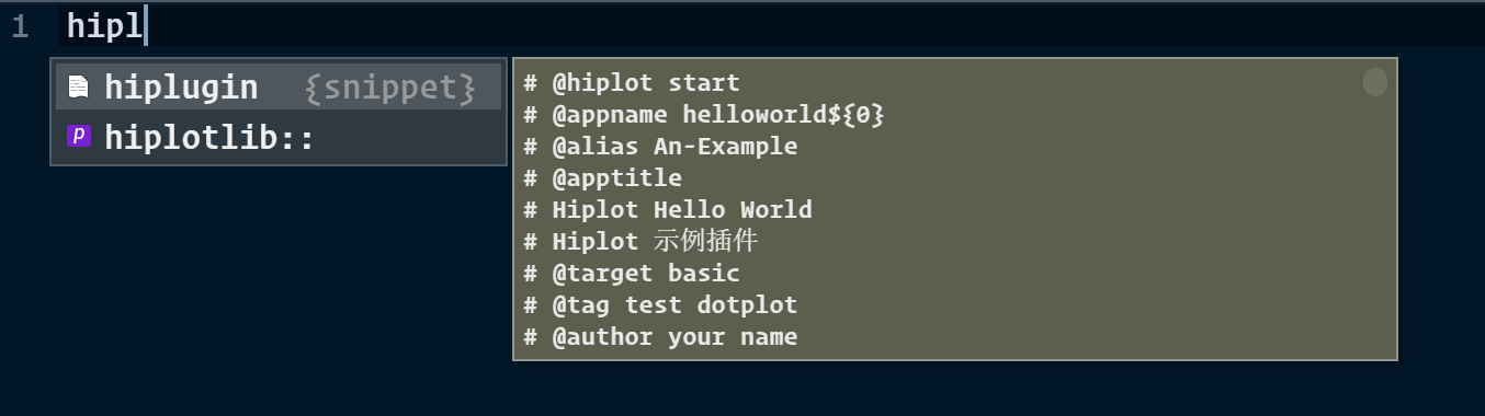
130 |
131 | 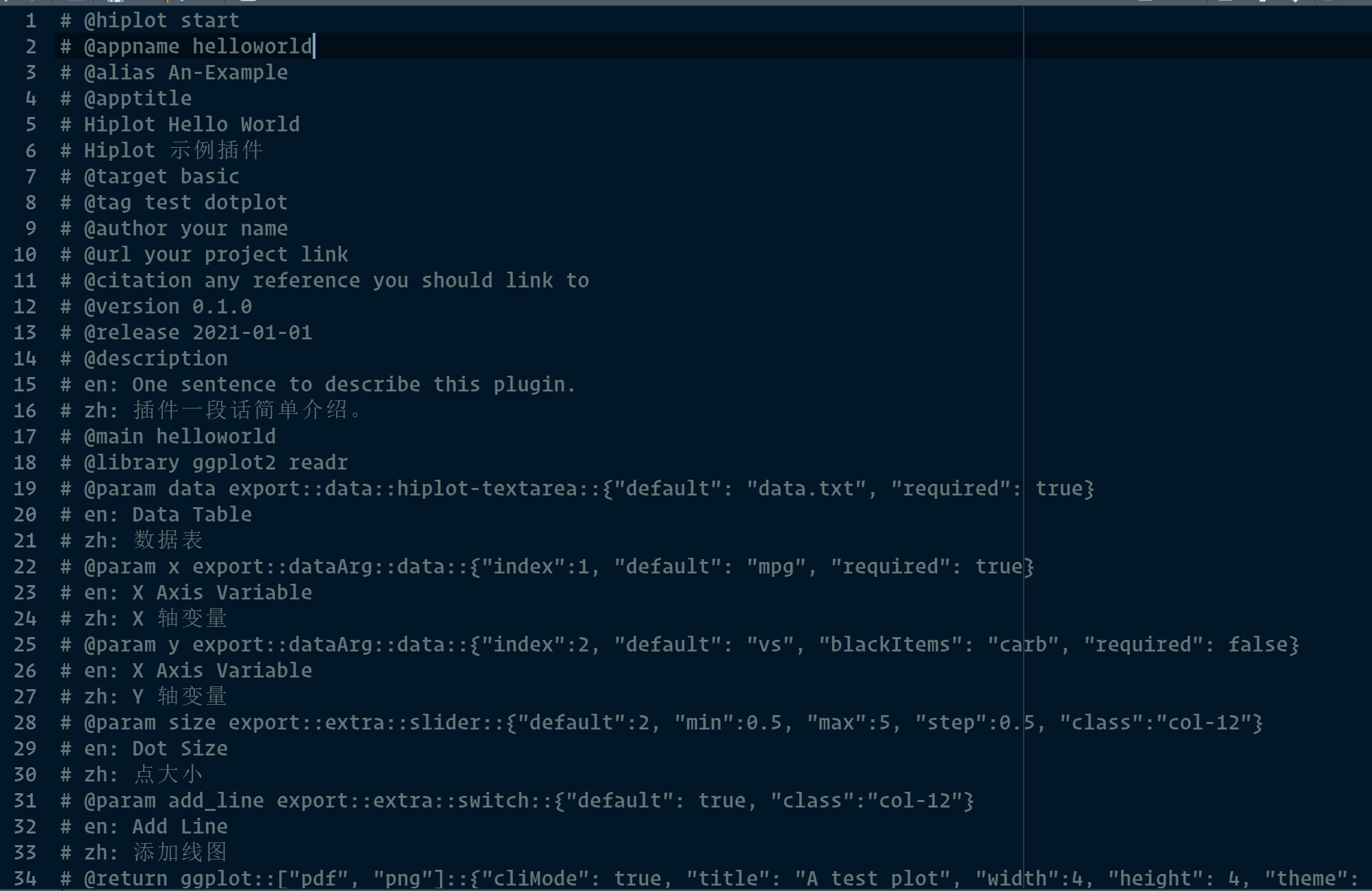
132 |
133 | #### VSCode snippet
134 |
135 | If you're prefer to using **VSCode**, we provide a snippet in [r.json](r.json), you can copy its content to VSCode R snippet.
136 |
137 | > If you have'nt use VSCode R snippet before, you can type `++P` to call the search panel and type `Configure User Snippet` and select `R` to open a `r.json` file.
138 |
139 | ### Step 2: implement the computation/visualization
140 |
141 | Now you open the `source.R` with your favorite editor (RStudio/VSCode/Vim), you will find a *helloworld* Hiplot plugin has been generated for you, this template plugin shows the core concept of Hisub and most common setting.
142 |
143 | ```R
144 | $ cat source.R
145 | # @hiplot start
146 | # @appname helloworld
147 | # @alias An-Example
148 | # @apptitle
149 | # Hiplot Hello World
150 | # Hiplot 示例插件
151 | # @target basic
152 | # @tag test dotplot
153 | # @author your name
154 | # @url your project link
155 | # @citation any reference you should link to
156 | # @version 0.1.0
157 | # @release 2021-01-01
158 | # @description
159 | # en: One sentence to describe this plugin.
160 | # zh: 插件一段话简单介绍。
161 | # @main helloworld
162 | # @library ggplot2 readr
163 | # @param data export::data::hiplot-textarea::{"default": "data.txt", "required": true}
164 | # en: Data Table
165 | # zh: 数据表
166 | # @param x export::dataArg::data::{"index":1, "default": "mpg", "required": true}
167 | # en: X Axis Variable
168 | # zh: X 轴变量
169 | # @param y export::dataArg::data::{"index":2, "default": "vs", "blackItems": "carb", "required": false}
170 | # en: X Axis Variable
171 | # zh: Y 轴变量
172 | # @param size export::extra::slider::{"default":2, "min":0.5, "max":5, "step":0.5, "class":"col-12"}
173 | # en: Dot Size
174 | # zh: 点大小
175 | # @param add_line export::extra::switch::{"default": true, "class":"col-12"}
176 | # en: Add Line
177 | # zh: 添加线图
178 | # @return ggplot::["pdf", "png"]::{"cliMode": true, "title": "A test plot", "width":4, "height": 4, "theme": "theme_bw"}
179 | # @data
180 | # # You can write the code to generate the example data
181 | # # "data.txt" described in parameter data, or you can
182 | # # omit this tag and submit prepared data files.
183 | # # File size <100Kb is recommended.
184 | # # 此处可以编写生成示例数据(建议小于 100Kb)的代码
185 | # # 示例数据文件需要跟数据表格参数对应起来
186 | # # 或者忽略该标签,提交已经准备好的示例数据
187 | # library(readr)
188 | # data("mtcars")
189 | # write_tsv(mtcars, "data.txt")
190 | # @hiplot end
191 |
192 | library(ggplot2)
193 | helloworld <- function(data, x, y, size = 2, add_line = TRUE) {
194 | if (y == "") stop("y must be provided!")
195 | p <- ggplot(data, aes_string(x = x, y = y))
196 | p <- p + geom_point(size = size)
197 | if (add_line) {
198 | p <- p + geom_line()
199 | }
200 | # Here export a ggplot object
201 | # Or the whole main function generate a basic R plot
202 | return(p)
203 | }
204 | ```
205 |
206 | > If you only write English, you can repeat English in the Chinese description part.
207 | >
208 | > Check [Hiplot tag list](#hiplot-tag-list) section for more description about supported Hiplot tags.
209 |
210 | We can divide the script contents into 2 parts:
211 |
212 | 1. The comment PART describe the metadata of this plugin and how the parameters map to a web widget (e.g., `select`) and their default values.
213 | 2. The code PART describe how to generate the result plot and we should **include the core plotting code in a function**.
214 |
215 | > **NOTE**: we use tag`@xxx` to recognize the useful information. HiSub **will only parse** the comments between `@hiplot start` and `@hiplot end`. And only the parameters with `export::` will be parsed.
216 |
217 | With the R script, we can generate the Hiplot plugin with command:
218 |
219 | ```sh
220 | $ hisub source.R helloword
221 | Using library: /Users/wsx/Library/R
222 | HiSub version 0.4
223 | Copyright (c) 2021 Hiplot (https://hiplot.cn/)
224 | ========================
225 | Checking dependencies...
226 | Loading required package: pacman
227 | Done
228 | Checking input...
229 | Done
230 | Preprocessing R script source.R
231 | Done
232 | Parsing Hiplot tags...
233 | Generating example data file...
234 | Done
235 | Generating plugin files...
236 | Set example data
237 | data rows: 32
238 | esize: 1.2509765625
239 | - meta.json
240 | - data.json
241 | - ui.json
242 | - plot.R
243 | Styling 1 files:
244 | helloword/plot.R ℹ
245 | ────────────────────────────────────────
246 | Status Count Legend
247 | ✔ 0 File unchanged.
248 | ℹ 1 File changed.
249 | ✖ 0 Styling threw an error.
250 | ────────────────────────────────────────
251 | Please review the changes carefully!
252 | ALL operations done. Check output directory for generated plugin.
253 | ```
254 |
255 | HiSub accept as many as parameters you can put, but only the first will be treated as the R script (here is `source.R`) to parse.
256 |
257 | Others parameters:
258 |
259 | - The last argument should be a directory path for the plugin, typically it has the same name as your plugin name.
260 | - Other middle arguments will be treated as necessary files (like `README.md`) and copied to the destination directory (specified by the last argument).
261 |
262 | Now you got a helloworld plugin for Hiplot:
263 |
264 | ```sh
265 | $ tree helloword
266 | helloword
267 | ├── data.json
268 | ├── data.txt
269 | ├── meta.json
270 | ├── plot.R
271 | └── ui.json
272 |
273 | 0 directories, 5 files
274 | ```
275 | ### Step 3: preview the plugin
276 |
277 | Then you can submit the generated `data.json` and `ui.json` to (You can also read exmaples provided by this link and see how to set the parameter settings) to see how it works. For our "Hello World", it looks like:
278 |
279 | 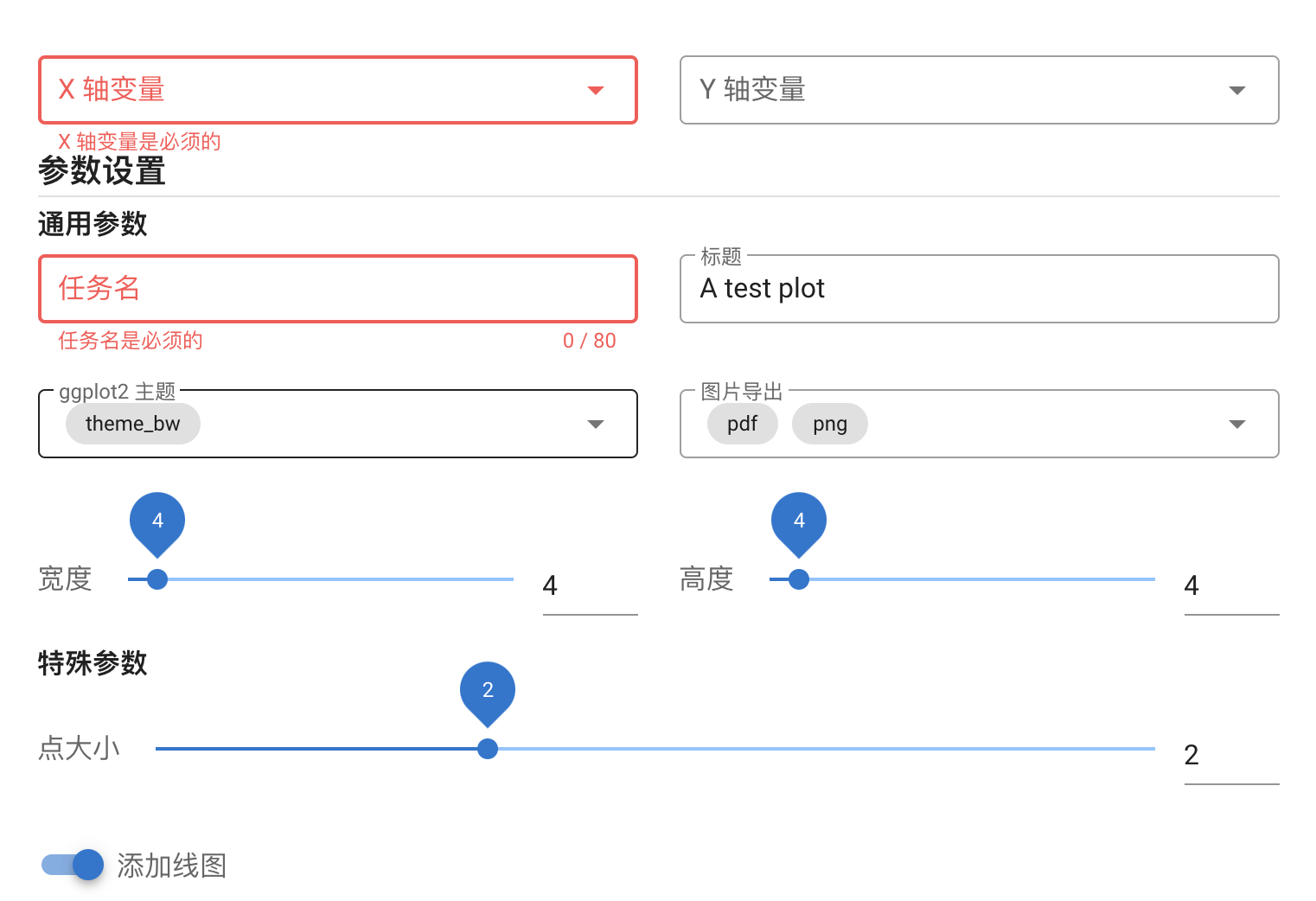
280 |
281 | ### Step 4 (optional): local test
282 |
283 | If you want to test locally to see if your plugin works well, 'hicli' command would help you.
284 |
285 | #### Use hicli in terminal
286 |
287 | ```sh
288 | $ cd helloword
289 | $ # Check help
290 | $ hicli -h
291 | Using library: /Users/wsx/Library/R
292 | Usage: /usr/local/bin/hicli [options]
293 |
294 |
295 | Options:
296 | -i INPUTFILE, --inputFile=INPUTFILE
297 | input data
298 |
299 | -c CONFFILE, --confFile=CONFFILE
300 | configuration file
301 |
302 | -o OUTPUTFILEPREFIX, --outputFilePrefix=OUTPUTFILEPREFIX
303 | prefix of output plots
304 |
305 | -t TOOL, --tool=TOOL
306 | (e.g. heatmap))
307 |
308 | -m MODULE, --module=MODULE
309 | module name (e.g. basic)
310 |
311 | -s, --simple
312 | only loading core packages
313 |
314 | -e, --enableExample
315 | enable auto load example
316 |
317 | -h, --help
318 | Show this help message and exit
319 | ```
320 |
321 | Run the helloword plugin locally.
322 |
323 | ```sh
324 | $ hicli -i data.txt -c data.json -t helloword -m basic -e -s -o hwtest/helloword
325 |
326 | General packages cowplot, patchwork, extrafont, R.utils are loaded.
327 | mpg cyl disp hp drat wt qsec vs am gear carb
328 | 1 21.0 6 160 110 3.90 2.620 16.46 0 1 4 4
329 | 2 21.0 6 160 110 3.90 2.875 17.02 0 1 4 4
330 | 3 22.8 4 108 93 3.85 2.320 18.61 1 1 4 1
331 | 4 21.4 6 258 110 3.08 3.215 19.44 1 0 3 1
332 | 5 18.7 8 360 175 3.15 3.440 17.02 0 0 3 2
333 | 6 18.1 6 225 105 2.76 3.460 20.22 1 0 3 1
334 | [1] "hwtest/log/core-steps.log"
335 | [1] "hwtest/log/done.log"
336 | [1] ""
337 | ```
338 |
339 | > `-e` must be enabled to include and preprocess the example data.
340 |
341 | Result tree:
342 |
343 | ```sh
344 | $ tree hwtest
345 | hwtest
346 | ├── helloword.Rdata
347 | ├── helloword.pdf
348 | ├── log
349 | │ ├── core-steps.log
350 | │ ├── done.log
351 | │ ├── read-data.log
352 | │ └── read-params.log
353 | └── task.log
354 |
355 | 1 directory, 7 files
356 | ```
357 |
358 | Also a file `task.status.json` is available in current directory.
359 |
360 | #### If you prefer to use R console
361 |
362 | ```r
363 | library(hiplotlib)
364 | basedir = "/Users/wsx/Documents/GitHub/hiplugin-test/helloword"
365 | opt = list(inputFile = file.path(basedir, "data.txt"),
366 | confFile = file.path(basedir, "data.json"),
367 | outputFilePrefix = file.path(basedir, "hwtest/helloword"),
368 | tool = "helloword",
369 | module = "basic",
370 | simple = TRUE,
371 | enableExample = TRUE,
372 | help = FALSE)
373 | dir.create(dirname(opt$outputFilePrefix))
374 | dir.create(file.path(dirname(opt$outputFilePrefix), "log"))
375 | options(hiplotlib.script_dir = dirname(basedir))
376 | run_hiplot()
377 | ```
378 |
379 | ### Step 5: plugin submission
380 |
381 | Now you can submit your plugin via email () or GitHub by pull request.
382 |
383 | ## More examples
384 |
385 | - [ezcox](https://github.com/hiplot/hiplotlib/tree/master/inst/hisub_examples/ezcox.R) -
386 | - [pcatools](https://github.com/hiplot/hiplotlib/tree/master/inst/hisub_examples/pcatools.R) -
387 |
388 | More information about UI design and setting can be found at .
389 |
390 | ## Hiplot tag list
391 |
392 | This part describes supported Hiplot tags.
393 |
394 | - `@hiplot`, 1 line, seperates the useful comments parsed by **HiSub**, only `start` and `end` are valid.
395 | - `@appname`, 1 line, set your plugin name (cannot have space, it will be used to set the plugin URL on hiplot).
396 | - `@apptitle`, 3 lines, set your plugin title.
397 | - The 2nd line set English title.
398 | - The 3rd line set Chinese title.
399 | - `@target`: 1 line, where the target url should be deployed to, includes `basic`, `advance`, `clinical-tools`, etc.
400 | - `@tag`: 1 line, tags for your plugin, seperated by space.
401 | - `@author`: 1 line, your name.
402 | - `@url`: 1 line, your project link, like GitHub for your plugin (**Optional**).
403 | - `@citation`: many lines, your reference or how to cite you (**Optional**).
404 | - `@version`: 1 line, the version of this plugin.
405 | - `@release`: 1 line, the release date of this version.
406 | - `@description`: many lines, briefly describe the plugin.
407 | - For English, you should start the line with `en:`.
408 | - For Chinese, you should start the line with `zh:`.
409 | - `@main`: 1 line, the main function to call for plotting.
410 | - `@library`: 1 line, required packages for your plugin, so Hiplot team can check if they are installed.
411 | - `@param`: many lines. From the 2nd line, it is same as `@description`. For the 1st line, it has the rules:
412 | - ` export::::::`
413 | - All `param_name`s are used to describe the parameters in the main function, here is `hello world()`.
414 | - `param-type` can be data (for data table), dataArg (for selecting column names in a data table), extra (custom parameters in your main function).
415 | - `widget-type` can be slider, switch, select, autocomplete, color-picker, text-field. More list and control see . You can see existing Hiplot plugin how to use config the widgets.
416 | - `param_setting` (JSON format) depends on the `widget-type`. In most common cases, a `default` item is supported to set default value for the parameter, others items will be passed to front end for setting widget UI and behavior.
417 | - `@return`: 1line, it has the rules:
418 | - `::::`
419 | - `output-type` can be `ggplot`, `plot` (for plots not generated by ggplot) and `directory` (outputing a whole directory, you need read docs for more).
420 | - `output-format` (JSON format) sets the figure output format like PDF, PNG, etc.
421 | - `output-setting` (JSON format) corresponds to default general parameters in a plot which provided in Hiplot UI but cannot be mapped to parameters of the main functions, like `title`, `palette`, `theme`, `width` and `height` of the plot, etc. (`cliMode` is suggested enable, it works faster for simple plugin).
422 | - `@data`: many line, it contains code to generate example data described in data table parameters (**Optional**).
423 |
424 | ## Utils of Hiplotlib
425 |
426 | Hiplotlib provides configuration variables and a lot of function families to execute the Hiplot plugin analysis worklfow and help to build a better plugin without writing too-many custom functions. You can directly use the features to custom output plots.
427 |
428 | | Variable/function | Description |
429 | | :-------------------------- | ------------------------------------------------------------ |
430 | | .conf | Mocked global objects to inherit web UI options/settings for plugin developer |
431 | | .opt | Mocked global objects to inherit web UI options/settings for plugin developer |
432 | | add_alpha | Add alpha to color |
433 | | alter_fun | Prestored settings and functions related to ggplot2 or plots |
434 | | brewer_palette_names | Prestored settings and functions related to ggplot2 or plots |
435 | | brewer_pal_update | Prestored settings and functions related to ggplot2 or plots |
436 | | capitalize | Capitalize a string |
437 | | cb_palette | Prestored settings and functions related to ggplot2 or plots |
438 | | choose_ggplot_theme | Prestored settings and functions related to ggplot2 or plots |
439 | | colname2data | Reset 'colnames' of a data frame |
440 | | col_fun_cont | Prestored settings and functions related to ggplot2 or plots |
441 | | col_tag | Prestored settings and functions related to ggplot2 or plots |
442 | | custom_color_filter | Prestored settings and functions related to ggplot2 or plots |
443 | | data_arg_preprocess | Preprocess the data argument from conf object |
444 | | deploy | Deploy Command Line Interface to System Local Path |
445 | | draw_map | Prestored settings and functions related to ggplot2 or plots |
446 | | export | Functions and utilities to export hiplot output |
447 | | export_directory | Functions and utilities to export hiplot output |
448 | | export_htmlwidget | Functions and utilities to export hiplot output |
449 | | export_plotly | Functions and utilities to export hiplot output |
450 | | export_pptx | Functions and utilities to export hiplot output |
451 | | export_single | Functions and utilities to export hiplot output |
452 | | get_hiplot_color | Prestored settings and functions related to ggplot2 or plots |
453 | | ggplot2 | Prestored settings and functions related to ggplot2 or plots |
454 | | ggplot2_themes | Prestored settings and functions related to ggplot2 or plots |
455 | | ggplot2_themes2 | Prestored settings and functions related to ggplot2 or plots |
456 | | ggsci_palette_length | Prestored settings and functions related to ggplot2 or plots |
457 | | ggsci_palette_names | Prestored settings and functions related to ggplot2 or plots |
458 | | gg_color_default | Prestored settings and functions related to ggplot2 or plots |
459 | | globs | Functions to manage the global setting objects |
460 | | globs_get | Functions to manage the global setting objects |
461 | | globs_list | Functions to manage the global setting objects |
462 | | globs_set | Functions to manage the global setting objects |
463 | | graf_palette_names | Prestored settings and functions related to ggplot2 or plots |
464 | | hiplotlib | hiplotlib package |
465 | | html2pdf | Functions and utilities to export hiplot output |
466 | | import | Functions and utilities related to data import |
467 | | import_images_to_pdf | Functions and utilities to export hiplot output |
468 | | list_same_string_position | Get the same characters in two strings |
469 | | merge_pdfs | Functions and utilities to export hiplot output |
470 | | mut_cols | Prestored settings and functions related to ggplot2 or plots |
471 | | new_task_step | Functions and utilities related to hiplot task |
472 | | parse_file_link | Functions and utilities to export hiplot output |
473 | | pdf2image | Functions and utilities to export hiplot output |
474 | | pdfs2image | Functions and utilities to export hiplot output |
475 | | position_type | Prestored settings and functions related to ggplot2 or plots |
476 | | prism_palette_names | Prestored settings and functions related to ggplot2 or plots |
477 | | read_data | Functions and utilities to export hiplot output |
478 | | return_ggplot_theme | Prestored settings and functions related to ggplot2 or plots |
479 | | return_hiplot_palette | Prestored settings and functions related to ggplot2 or plots |
480 | | return_hiplot_palette_color | Prestored settings and functions related to ggplot2 or plots |
481 | | run_hiplot | Run hiplot |
482 | | run_task_step | Functions and utilities related to hiplot task |
483 | | set_complex_general_theme | Prestored settings and functions related to ggplot2 or plots |
484 | | set_extra_pkgs | Set extra R packages before starting plugin |
485 | | set_factors | Set a vector to a factor |
486 | | set_general_pkgs | Set general R packages before starting plugin |
487 | | set_global_confs | Check and update global setting before starting plugin |
488 | | set_global_options | Set R global options before starting plugin |
489 | | set_palette_theme | Prestored settings and functions related to ggplot2 or plots |
490 | | split_pdfs | Functions and utilities to export hiplot output |
491 | | system_safe | Run system commands |
492 | | task | Functions and utilities related to hiplot task |
493 | | transform | Transform value |
494 | | transform_val | Transform value |
495 | | transparentColor | Prestored settings and functions related to ggplot2 or plots |
496 | | update_task_status | Functions and utilities related to hiplot task |
497 |
498 | > Updated at 2022/5/6
499 |
500 | ## Bug report | feature request
501 |
502 | Please file an issue to .
503 | ## Copyright
504 |
505 | © 2020-2022 Hiplot team
506 |
507 |
--------------------------------------------------------------------------------
/zh/usage/basic/README.md:
--------------------------------------------------------------------------------
1 | # 基础模块
2 |
3 | ## [面积图](/basic/area)
4 |
5 | - 简介
6 |
7 | 面积图是一种基于折线图并以图形方式显示定量数据的图形。轴和线之间的区域通常用颜色、纹理和图案来强调。
8 |
9 | - 案例数据分析
10 |
11 | 载入数据为 x 轴数值和 y 轴数值。
12 |
13 | - 案例统计图形解读
14 |
15 | 不同颜色代表不同组的面积图。
16 |
17 | ## [3D 柱状图](/basic/barplot-3d)
18 |
19 | - 简介
20 |
21 | 三维柱状图用于为数据提供三维外观。 第三维通常出于美学原因而使用,但其不能改善数据的读取。 仍旨在显示离散类别之间的比较。
22 |
23 | - 案例数据分析
24 |
25 | 载入数据为不同治疗方案中不同剂量药物作用效果数据。
26 |
27 | - 案例统计图形解读
28 |
29 | 该三维柱状图展示了不同治疗组(组 1 ~ 组 4)分别用低、中、高剂量进行治疗时,不同的治疗效果。组 1 使用中剂量治疗时效果最好,组 2 使用高剂量治疗时效果最好,组3使用剂量治疗时无较大差距,组 4 使用高剂量治疗时效果最好。
30 |
31 | - 特殊参数
32 |
33 | 俯仰角:正值越大,表示趋于从三维图形顶端向下观测;负值越大,表示趋于从三维图形底端向上观测。
34 |
35 | 水平旋转角度:三维图形水平旋转的角度。
36 |
37 | ## [颜色组柱状图](/basic/barplot-color-group)
38 |
39 | 颜色组柱状图可以用于分组展示数据值,并按顺序标注不同颜色,常应用于 GO/KEGG 通路富集分析结果的可视化。
40 |
41 | - 数据表格(三列):
42 |
43 | Term | 条目名称,如 GO/KEGG 通路名称
44 |
45 | Count | 条目的数值大小,如某通路富集到的基因数
46 |
47 | Type | 该通路所属大类:如 BP/MF/CC/KEGG
48 |
49 | - 特殊参数:
50 |
51 | 展示数目 | 用于控制柱状图中各分组所展示的最多条目数量,如设置为 4,则只取 Type 各分组的分别前 4 条记录
52 | ## [误差线条形图2](/basic/barplot-errorbar2)
53 |
54 | - ### 功能介绍
55 |
56 | 带误差线和误差组的条形图。
57 | ## [误差线条形图](/basic/barplot-errorbar)
58 |
59 | - ### 功能介绍
60 |
61 | 带误差线和误差组的条形图。
62 | ## [渐变柱状图](/basic/barplot-gradient)
63 |
64 | - 简介
65 |
66 | 同气泡图相似,不过是在柱状图的基础上,用颜色渐变的长方形同时展示两个变量的可视化图形。
67 |
68 | - 案例数据分析
69 |
70 | 第一列为Go Term(Go语言编号),第二列为基因数,第三列输入pvalue。
71 |
72 | - 案例统计图形解读
73 |
74 | 如图示,蓝色为低pvalue颜色,红色为高pvalue颜色,随着pvalue增大颜色由蓝向红渐变。横坐标表示基因数目。
75 |
76 | - 特殊参数
77 |
78 | 展示数目:展示Go Term中Go id数量
79 |
80 | 水平:开启时纵坐标为Go id,横坐标为数值,图形呈现水平排列的长方形。关闭时横纵坐标对调,图形呈现纵向排列的长方形。
81 |
82 | 低数值颜色:表示低pvalue所显示的颜色
83 |
84 | 高数值颜色:表示高pvalue所显示的颜色
85 | ## [多变量线图](/basic/barplot-line-multiple)
86 |
87 | - ### 功能介绍
88 |
89 | 在一个图表中显示多个条形图或线形图。
90 |
91 | - ### 数据结构
92 |
93 | 具有多列数据(数字)的数据框。
94 |
95 | - ### 参数详解
96 |
97 | **主要参数**
98 |
99 | Title: 图像的主标题(部分图像可替换默认标题)
100 |
101 | Theme: 图像主题(由ggplot2提供的主题)
102 |
103 | Color Palette: 图像配色(由ggsci提供的主流期刊优秀配色)
104 |
105 | Font Family: 字体(如主流期刊规定的Time New Romas)
106 |
107 | Width: 输出图像的宽度(默认为英寸如标准为12 x 7 inch)
108 |
109 | Height: 输出图像的高度(默认为英寸如标准为12 x 7 inch)
110 |
111 | Alpha: 元素的透明度(0-1,0表示透明,1表示不透明)
112 |
113 |
114 | **重要参数**
115 |
116 | Legend Position: 图例在图像中的位置
117 |
118 | Legend Direction: 图例中多个元素的排列方式(横向或纵向)
119 |
120 | Legend Title Size: 图例主标题大小
121 |
122 | Legend Text Size: 图例中元素文本的大小
123 |
124 |
125 | Axis Title Size: 图像坐标轴标题的大小
126 |
127 | Axis Font Size: 图像坐标轴刻度字体的大小
128 |
129 | Axis Text Angle: 图像坐标轴文本的角度
130 |
131 | Axis Adjust: 图像坐标轴文本的距离(微调)
132 |
133 |
134 | **特殊参数**
135 |
136 | Plot Type: 图像的类型(线图或条形图)
137 |
138 | Line Size: 线图对应线条的宽度
139 |
140 | Point Size: 数据点的大小
141 |
142 |
143 | ## [柱状图](/basic/barplot)
144 |
145 | - 简介
146 |
147 | 柱状图是一种以长方形的长度表示数据值大小的统计图表。
148 |
149 | - 案例数据分析
150 |
151 | 载入数据为不同治疗方案中不同剂量药物作用效果数据。
152 |
153 | - 案例统计图形解读
154 |
155 | 条形图用于显示带有矩形条的类别数据, 矩形条的高度或长度与它们所代表的值成比例。条形图可以垂直或水平绘制。条形图显示了离散类别之间的比较。 图表的一个轴显示要比较的特定类别,另一个轴代表测量值。 一些条形图显示的条形也可显示多个测量变量的值。该条形图展示了不同治疗组(组 1 ~ 组 4)分别用低、中、高剂量进行治疗时,不同的治疗效果。组 1 使用中剂量治疗时效果最好,组 2 使用高剂量治疗时效果最好,组 3 使用剂量治疗时无较大差距,组 4 使用高剂量治疗时效果最好。
156 |
157 | - 特殊参数
158 |
159 | 叠加类型:dodge 表示横向罗列,stack 表示上下叠加
160 |
161 | 水平:互换类别轴与测量值轴的位置
162 |
163 | 添加数字标签:标注数值
164 |
165 | ## [豆荚图](/basic/beanplot)
166 |
167 | - 简介
168 |
169 | 豆荚图是一种描述一组数据分布特征的方法。
170 |
171 | - 案例数据分析
172 |
173 | 载入数据为数据集 (不同治疗方案的治疗效果数据)。
174 | ## [蜜蜂群图](/basic/beeswarm)
175 |
176 | - 简介
177 |
178 | 蜜蜂群图是一种类似蜜蜂群,样本间互不干涉的列散点图。
179 |
180 | - 案例数据分析
181 |
182 | 载入数据为不同分组及其数据。
183 |
184 | - 案例统计图形解读
185 |
186 | 不同颜色表示不同组群 ,点表示数据。
187 |
188 | ## [大样本相关性热图 (Corrplot)](/basic/big-corrplot)
189 |
190 | - 简介
191 |
192 | 相关性热图是一种分析多个变量,两两之间相关性的图形。
193 |
194 | - 案例数据分析
195 |
196 | 载入数据为基因名称及每个样本的表达量。
197 |
198 | - 案例统计图形分析
199 |
200 | 红色系表示两个基因之间呈正相关,蓝色系表示两个基因之间呈负相关,每一格中的数字表示相关系数。
201 |
202 | ## [多百分比图](/basic/multi-percentage)
203 |
204 | - 简介
205 |
206 | 显示多个双变量关系。
207 |
208 | ## [箱式图](/basic/boxplot)
209 |
210 | - 简介
211 |
212 | 箱形图是一种通过四分位数图形象化地描述一组数据分布特征的方法。
213 |
214 | - 案例数据分析
215 |
216 | 载入数据为数据集 (不同治疗方案的治疗效果数据)。
217 |
218 | - 案例统计图形分析
219 |
220 | 横坐标表示几组不同的数据,纵坐标分别表示各组数据的四分位数;即方框上、中、下的横线分别代表上四分位数,中位数,下四分位数;上下方线段代表的数值分别指数据最大值和最小值,方框以外的点代表离群值。图示上方数值表示两两变量间的 P 值,可认为治疗方案 1 中,中剂量组同低剂量组疗效有显著差异,以此类推。
221 |
222 | - 特殊参数
223 |
224 | P 值展示形式:value 表示数值,signif 表示 "\*" 的数量,no 表示不展示 P 值
225 |
226 | 添加散点:将数值表示的点标明出来
227 |
228 | ## [气泡图](/basic/bubble)
229 |
230 | - 简介
231 |
232 | 气泡图是在散点图的基础上,用气泡的大小来展示第三个变量,从而能够同时对三个变量进行对比分析的统计图表。
233 |
234 | - 案例数据分析
235 |
236 | 载入数据为 GO Term, Gene Ridio,基因数和 P 值。
237 |
238 | - 案例统计图形分析
239 |
240 | x 轴表示 Gene Ridio,y 轴是 GO Term; 点的大小表示基因数,点的颜色代表 P 值的高低。
241 |
242 | - 特殊参数
243 |
244 | 展示数目:显示气泡的数量
245 |
246 | 颜色主题:显示 P 值的颜色主题
247 |
248 | ## [凹凸图](/basic/bumpchart)
249 |
250 | - Introduction
251 |
252 | 凹凸图可以用于展示多组数值变化情况。
253 | ## [模型评估曲线图](/basic/calibration-curve)
254 |
255 | - ### 功能介绍
256 |
257 | 校准曲线用于评估一致性/校准,即预测值和实际值之间的差异。
258 |
259 | - ### 数据结构
260 |
261 | 多列数据的数据帧(数字允许NA)。ie生存数据(状态为0和1)。
262 |
263 | - ### 参数详解
264 |
265 | **主要参数**
266 |
267 | Title: 图像的主标题(部分图像可替换默认标题)
268 |
269 | Theme: 图像主题(由ggplot2提供的主题)
270 |
271 | Color Palette: 图像配色(由ggsci提供的主流期刊优秀配色)
272 |
273 | Font Family: 字体(如主流期刊规定的Time New Romas)
274 |
275 | Width: 输出图像的宽度(默认为英寸如标准为12 x 7 inch)
276 |
277 | Height: 输出图像的高度(默认为英寸如标准为12 x 7 inch)
278 |
279 | Alpha: 元素的透明度(0-1,0表示透明,1表示不透明)
280 |
281 |
282 | **重要参数**
283 |
284 | Legend Position: 图例在图像中的位置
285 |
286 | Legend Direction: 图例中多个元素的排列方式(横向或纵向)
287 |
288 | Legend Title Size: 图例主标题大小
289 |
290 | Legend Text Size: 图例中元素文本的大小
291 |
292 |
293 | Axis Title Size: 图像坐标轴标题的大小
294 |
295 | Axis Font Size: 图像坐标轴刻度字体的大小
296 |
297 | Axis Text Angle: 图像坐标轴文本的角度
298 |
299 | Axis Adjust: 图像坐标轴文本的距离(微调)
300 |
301 |
302 | **特殊参数**
303 |
304 | Model: 模型计算的方法(默认为线性拟合模型)
305 |
306 | CMethod: 检查模型的方法(默认为KM算法)
307 |
308 | Method: 校准的方法(默认为Boot方法)
309 |
310 | Time(Day): 时间,支持时间单位为天(默认365天)
311 |
312 |
313 | ## [卡方与 Fisher 检验](/basic/chi-square-fisher)
314 |
315 | - 简介
316 |
317 | 卡方与 Fisher 检验可用于分类变量频数差异检验,该工具将自动选择卡方和 Fisher 确切性检验统计方法。
318 |
319 | - 数据表
320 |
321 | 数据表支持两种格式:列联表(示例 1)和单行记录表(示例 2)
322 |
323 | - 额外参数
324 |
325 | 循环方法 | 该工具会生成所有可以比较的排列组合,然后通过遍历分别检验两组间差异,可选按列联表的行和列遍历
326 |
327 | 添加均值 | 添加均值行加入检验遍历
328 |
329 | 添加中位数 | 添加中位数行加入检验遍历
330 | ## [弦图](/basic/chord)
331 |
332 | - ### 功能介绍
333 |
334 | 复杂的数据关系交互作用以和弦图的形式表现出来。
335 |
336 |
337 | - ### 数据结构
338 |
339 | 基因与通路或基因本体相互作用的数据框架或矩阵。
340 |
341 | - ### 参数详解
342 |
343 | **主要参数**
344 |
345 | Title: 图像的主标题(部分图像可替换默认标题)
346 |
347 | Theme: 图像主题(由ggplot2提供的主题)
348 |
349 | Color Palette: 图像配色(由ggsci提供的主流期刊优秀配色)
350 |
351 | Font Family: 字体(如主流期刊规定的Time New Romas)
352 |
353 | Width: 输出图像的宽度(默认为英寸如标准为12 x 7 inch)
354 |
355 | Height: 输出图像的高度(默认为英寸如标准为12 x 7 inch)
356 |
357 | Alpha: 元素的透明度(0-1,0表示透明,1表示不透明)
358 |
359 |
360 | **重要参数**
361 |
362 | Legend Position: 图例在图像中的位置
363 |
364 | Legend Direction: 图例中多个元素的排列方式(横向或纵向)
365 |
366 | Legend Title Size: 图例主标题大小
367 |
368 | Legend Text Size: 图例中元素文本的大小
369 |
370 |
371 | Axis Title Size: 图像坐标轴标题的大小
372 |
373 | Axis Font Size: 图像坐标轴刻度字体的大小
374 |
375 | Axis Text Angle: 图像坐标轴文本的角度
376 |
377 | Axis Adjust: 图像坐标轴文本的距离(微调)
378 |
379 |
380 | **特殊参数**
381 |
382 | Dist Name: 标签与弦图的距离
383 |
384 | Circle Width: 弦图环状的边框的宽度
385 |
386 | Label Distance: 标签的距离
387 |
388 | Link Visible: 弦图中纽带是否展示
389 |
390 | Scale: 弦图是否按元素多少自由缩放占比展示
391 |
392 |
393 | [复合热图](/basic/complex-heatmap)
394 |
395 | - 简介
396 |
397 | 一个多组学插件同时绘制热图、注释和突变信息。
398 |
399 | - 数据参数列
400 |
401 | 第一个值指定突变开始列。第二个值指定热图表达矩阵开始列。## [等高线图(矩阵)](/basic/contour-matrix)
402 |
403 | - 简介
404 |
405 | 等高图(矩阵)是一种以二维形式展示三维数据的图形。
406 |
407 | - 案例数据分析
408 |
409 | 载入数据为一个矩阵。
410 |
411 | - 案例统计图形分析
412 |
413 | 黄色代表最高,深紫色代表最低,高度刻度范围是90-190。
414 |
415 | ## [等高线图 (XY)](/basic/contour-xy)
416 |
417 | - 简介
418 |
419 | 等高线图 (XY) 是一种通过等高线反映数据密集程度的数据处理方式。
420 |
421 | - 案例数据分析
422 |
423 | 载入数据为两个变量
424 |
425 | - 案例统计图形分析
426 |
427 | 正如地理上的等高线代表不同高度一样,等高线图上的不同等高线代表不同密度,越靠中心,等高线圈越小,代表其区域数据密度程度越高。如:黄色区域数据密集程度最高,而蓝色区域数据密集程度最低。
428 |
429 | ## [相关性热图](/basic/cor-heatmap)
430 |
431 | - 简介
432 |
433 | 相关性热图是一种分析多个变量,两两之间相关性的图形。
434 |
435 | - 案例数据分析
436 |
437 | 载入数据为基因名称及每个样本的表达量。
438 |
439 | - 案例统计图形分析
440 |
441 | 红色系表示两个基因之间呈正相关,蓝色系表示两个基因之间呈负相关,每一格中的数字表示相关系数。
442 |
443 | - 特殊参数
444 |
445 | 相关性计算(行/列):row 表示按照行进行相关性计算,col 表示按照列进行相关性计算。
446 |
447 | 选择展示部分:upper 表示显示左上角图形,lower 表示显示右下角图形,full 表示显示全景图片。
448 |
449 | 形状:circle 表示每个格子内的图形是圆圈,square 表示每个格子内的图形是正方形。
450 |
451 | 排序:按照得到的相关性系数进行排序。
452 |
453 | ## [简单可变相关热图](/basic/cor-heatmap-simple)
454 |
455 | 该插件提供了一个简单的相关热图可视化功能,它主要用于快速生成相关热图并支持在不同的轴上展示特定的变量。
456 |
457 | 核心参数:
458 |
459 | - X 轴:设置显示在 X 轴的变量。
460 | - Y 轴:设置显示在 X 轴的变量。
461 |
462 | 更多信息查看[内部函数实现](https://shixiangwang.github.io/sigminer/reference/show_cor.html)。## [相关性热图 (Corrplot)](/basic/corrplot)
463 |
464 | - 简介
465 |
466 | 相关性热图是一种分析多个变量,两两之间相关性的图形。
467 |
468 | - 案例数据分析
469 |
470 | 载入数据为基因名称及每个样本的表达量。
471 |
472 | - 案例统计图形分析
473 |
474 | 红色系表示两个基因之间呈正相关,蓝色系表示两个基因之间呈负相关,每一格中的数字表示相关系数。
475 |
476 | ## [ggplot2 词云](/basic/ggwordcloud)
477 |
478 | - 简介
479 |
480 | 词云是通过形成“关键词云层”或“关键词渲染”,对网络文本中出现频率较高“关键词”进行可视化。
481 |
482 | - 案例数据分析
483 |
484 | 载入数据名词和名词频数。
485 |
486 | - 案例统计图形解读
487 |
488 | 图示显示心形图片,按照名词频数的大小显示其在词云图中的占比。
489 |
490 | - 特殊参数
491 |
492 | 渐变模式:更改颜色为渐变
493 |
494 | 渐变深色:词频低的名词为深色
495 |
496 | 渐变高亮色:词频高的名词为浅色
497 | ## [系统树图](/basic/dendrogram)
498 |
499 | - 简介
500 |
501 | 系统树图是一种以树的形状表示的图。这种图表在不同情景有不同的含义。如:在层次聚类中,说明了相应分析产生的聚类的排列。在生物信息中,它显示基因或样本的聚集,有时在热图的边缘。
502 |
503 | - 案例数据分析
504 |
505 | 载入数据为基因名称及其对应的基因表达值。
506 |
507 | - 案例统计图形解读
508 |
509 | 该图如同垂直 90° 的树,M1-M10 表示树根,树枝向右生长聚合,形成树枝树干。可以看出,该图先后生成 2 类,4 类,以此类推。
510 |
511 | - 特殊参数
512 |
513 | 分支数:
514 |
515 | 距离计算方法:更改计算树距离的方法
516 |
517 | 树的外形:更改树的形状
518 |
519 | 添加标签颜色:聚类后使样本相近的样本名称颜色相近
520 |
521 | ## [镜像密度图和直方图](/basic/density-hist-mirror)
522 |
523 | - 简介
524 |
525 | 镜像密度图和直方图是一种使用上下双侧绘制方法用来观察连续型变量分布的图形
526 | ## [密度图-直方图](/basic/density-histogram)
527 |
528 | - 简介
529 |
530 | 使用密度图或直方图展示数据分布。
531 | ## [密度图](/basic/density)
532 |
533 | - 简介
534 |
535 | 核密度图是一种用来观察连续型变量分布的图形。
536 |
537 | - 案例数据分析
538 |
539 | 载入数据为数据集 (不同治疗方案治疗效果数据)。
540 |
541 | - 案例统计图形分析
542 |
543 | 不同颜色表示不同分组,横轴表示数值,纵轴表示频率。
544 |
545 | - 特殊参数
546 |
547 | 堆积图形:
548 |
549 | ## [扩散映射](/basic/diffusion-map)
550 |
551 | - 简介
552 |
553 | 扩散映射(diffusion-map)是一种非线性降维算法,可以用于可视化发育轨迹。
554 | ## [双侧标准化图](/basic/diverging-scale)
555 |
556 | - 简介
557 |
558 | 双侧标准化图是一种将连续的,定量的输入映射到连续的固定的插值器上的图形。
559 |
560 | - 案例数据分析
561 |
562 | 第一列为模型名称列表,其余列输入相关指标及对应数值。
563 |
564 | - 案例统计图形解读
565 |
566 | 图示横轴表示hp数据,纵轴表示模型名称(分类),红色表示超过平均值的模型,蓝色表示低于平均值的模型,数据是按照大小赋值于 2 的比例尺上面。
567 |
568 | - 特殊参数
569 |
570 | 类型:lollipop 表示中轴线两侧绘制滑珠图;bar 表示中轴线两侧绘制条形图。
571 |
572 | 标准化:标准化打开是将数据进行标准化后,显示在±2的比例尺上,标准化关闭显示纵向滑珠图和柱状图。
573 |
574 | 线条大小:随着右拉数值增大,从纵轴延伸出去的红蓝线增粗。
575 |
576 | 点大小:随着右拉数值增大,红蓝线终点处定位横纵数值的点变大。
577 |
578 | 颜色:表示线条颜色,默认红色为正向线条颜色,蓝色为负向线条颜色。
579 |
580 | ## [环形图](/basic/donut)
581 |
582 | - 简介
583 |
584 | 环形图是饼图的一种变体,它有一个允许包含数据整体额外信息的空白中心。且与饼图目的一致,都是用来说明数据比例。
585 |
586 | - 案例数据分析
587 |
588 | 载入数据为不同分组及其数据。
589 |
590 | - 案例统计图形解读
591 |
592 | 不同颜色表示不同组群 ,不同面积表示数据及占比。
593 |
594 | ## [滑珠图](/basic/dotchart)
595 |
596 | - 简介
597 |
598 | 滑珠图是一种珠子在柱上滑行的图形,是条形图与散点图的叠加。
599 |
600 | - 案例数据分析
601 |
602 | 载入数据为基因名称及其对应的基因表达值和分组。
603 |
604 | - 案例统计图形分析
605 |
606 | 每种颜色表示不同的分组,能够直观了解不同基因表达值的差异。
607 |
608 | ## [双Y轴图](/basic/dual-y-axis)
609 |
610 | - 简介
611 |
612 | 双Y轴图可以将两组数量级较大的数据放在同一个图中进行展示。
613 |
614 | - 案例数据分析
615 |
616 | 载入数据为分为三列,第一列是x轴的数值,第二列为左侧Y轴的数值,第三列为右侧Y轴的数值。
617 |
618 | - 案例统计图形解读
619 |
620 | 案例数据中左侧Y轴比例尺量级在0-100的范围,而右侧Y轴比例尺则在0-1000。
621 |
622 | - 特殊参数
623 |
624 | 放缩系数:用于第二个Y轴比例尺的放缩
625 |
626 | 颜色一:第一条折线的颜色
627 |
628 | 颜色二:第二条折现的颜色
629 |
630 |
631 | ## [凹凸图](/basic/dumbbell)
632 |
633 | - Introduction
634 |
635 | 凹凸图可以用于展示数值变化情况。
636 | ## [简易配对图](/basic/easy-pairs)
637 |
638 | - 简介
639 |
640 | 显示一个矩阵图,用于查看多个变量的相关关系和数据分布。
641 |
642 | ## [SOM 模型可视化](/basic/easy-som)
643 |
644 | - 简介
645 |
646 | 建立 SOM 模型,并可视化结果
647 | ## [COX 模型森林图](/basic/ezcox)
648 |
649 | - 简介
650 |
651 | COX 模型森林图对 COX 模型构建风险森林图,以便于筛选变量的一种可视化图形。
652 |
653 | - 案例数据分析
654 |
655 | 载入数据为时间,生存结局及多个变量因素。
656 |
657 | - 案例统计图形解读
658 |
659 | 图示表格第一列表示变量及样本数,第二列森林图图示,第三列表示CI95%置信区间范围及其平均值和 P 值
660 |
661 | 森林图解读
662 |
663 | 中间垂直线表示无效线,横线表示该变量因素的95%置信区间,长短表示置信区间范围的大小,若某变量因素置信区间与无效线相交,则认为该变量因素无统计学意义,方块的位置是HR的点估计。
664 |
665 | age 因素为控制变量。
666 |
667 | ph.ecog 因素的发生率大于年龄因素的发生率,且 ph.ecog 因素会增加生存的发生(P < 0.001,有统计学意义)。
668 |
669 | sex 因素的发生率小于年龄因素的发生率,且 sex 因素会减少生存的发生(P = 0.002 < 0.05,有统计学意义)。
670 |
671 | - 特殊参数
672 |
673 | 合并模型:将多个变量因素整合进一个图标中。
674 |
675 | 去除控制变量:去除图表中 age 变量一行。
676 |
677 | 添加文字说明:在图标右下方标注标题。
678 |
679 | ## [扇形图](/basic/fan)
680 |
681 | - 简介
682 |
683 | 扇形图是旨在以所占扇形的大小清楚表示各组数据所占百分比的统计图表。
684 |
685 | - 案例数据分析
686 |
687 | 载入数据为不同分组及其数据。
688 |
689 | - 案例统计图形解读
690 |
691 | 不同颜色表示不同组群 ,不同面积表示数据及占比。
692 |
693 | - 特殊参数
694 |
695 | 显示占比:在不同分组旁显示其占比
696 |
697 | ## [鱼形图](/basic/fishplot)
698 |
699 | 详细信息: https://github.com/chrisamiller/fishplot
700 |
701 | - 数据表
702 |
703 | timepoints:为矩阵的每一列指定时间点
704 |
705 | parents:指定克隆之间的父母关系
706 |
707 | samplename:样品名称(支持多个样品)
708 |
709 | other:包含所有时间点所有克隆的肿瘤比例估计值的数值矩阵
710 |
711 | - 通用参数
712 |
713 | 颜色画板: 控制背景颜色
714 |
715 | 颜色画板 2: 控制克隆颜色
716 |
717 | - 额外参数
718 |
719 | 形状:形状类型
720 |
721 | 背景类型:提供背景类型的字符串
722 |
723 | 时间单位:时间点单位标签
724 |
725 | 描边宽度:多边形周围的边框线的宽度
726 |
727 | 左侧间距占比:第一个时间点左侧的增量数量。给出为总绘图宽度的一部分
728 |
729 | 竖线:添加时间点垂直线
730 |
731 | 克隆标签:添加克隆名称
732 |
733 | 校正缺失值:是否校正在非零值之间的时间点具有零值的克隆, 如果克隆再次出现,则克隆必须仍然存在
734 |
735 | 竖线颜色:时间点竖线颜色
736 |
737 | 描边颜色:形状的描边颜色
738 | ## [漏斗图 (Metafor)](/basic/funnel-plot-metafor)
739 |
740 | - 简介
741 |
742 | 可以用于分析 Meta 分析结果中潜在偏倚因子。
743 | ## [漏斗图](/basic/funnel-plot)
744 |
745 | - 简介
746 |
747 | 可以用于分析 Meta 分析结果中潜在偏倚因子。
748 | ## [甘特图](/basic/gantt)
749 |
750 | - 简介
751 |
752 | 甘特图是一种用来说明项目进度条形图。
753 |
754 | - 案例数据分析
755 |
756 | 载入数据为 4 个样本即四位患者,3 个项目即 3 种治疗方法,以及每种治疗方法的起止时间。
757 |
758 | - 案例统计图形解读
759 |
760 | 横轴表示时间进度,纵轴表示 4 位患者,3 种颜色表示 3 种治疗方法,该图可以观测到每位患者不同治疗方法使用的时间进度。
761 |
762 | ## [分布图](/basic/ggdist)
763 |
764 | - 简介
765 |
766 | 分布图是一种采用置信分布的可视化图形。
767 |
768 | - 案例数据分析
769 |
770 | 载入数据为 5 种条件及其对应的值。
771 |
772 | - 案例统计图形解读
773 |
774 | 图示给出的是条件下均值的置信度分布,可以看出 5 种条件下对应值的大致分布情况。
775 |
776 | ## [ggpubr-boxplot](/basic/ggpubr-boxplot)
777 |
778 |
779 | 如果你对参数设定有什么疑问,可以自己利用示例数据进行尝试和理解,如果还是不懂,可以查阅 或互联网材料。## [序列 LOGO](/basic/ggseqlogo)
780 |
781 | - 简介
782 |
783 | 序列 Logo 是一种用来描述结合位点序列模式的图形。
784 |
785 | - 案例数据分析
786 |
787 | 载入数据为多个转录因子在多个基因上的结合位点的序列。
788 |
789 | - 案例统计图形解读
790 |
791 | 采用 bits 计算的方式将一个结合位点序列展示在图表一列,可以清晰观测到不同序列占比较大的碱基。
792 |
793 | - 特殊参数
794 |
795 | 序列类型:dna 表示 DNA 序列,rna 表示 RNA 序列,aa 表示氨基酸序列。
796 |
797 | 序列颜色:不同碱基颜色。
798 |
799 | 方式类型:bits 表示采用 bits 公式展示不同碱基在最大值为 2 的纵坐标轴中的占比;prob 表示碱基占序列总体碱基的比例,并按占比展示在最大值为 1 的纵坐标轴中。
800 |
801 | ## [D3 词云](/basic/d3-wordcloud)
802 |
803 | - 简介
804 |
805 | 词云是通过形成“关键词云层”或“关键词渲染”,对网络文本中出现频率较高“关键词”进行可视化。
806 |
807 | - 案例数据分析
808 |
809 | 载入数据名词和名词频数。
810 |
811 | - 案例统计图形解读
812 |
813 | 按照名词频数的大小显示其在词云图中的占比。
814 |
815 | - 特殊参数
816 |
817 | 最小旋转:词条最小顺时针旋转角度
818 |
819 | 最大旋转:词条最大顺时针旋转角度
820 |
821 | 字体大小范围:限制词条字体大小
822 |
823 | 字间距:词条字体间距
824 | ## [分组比较热图](/basic/group-comparison)
825 |
826 | 这个插件提供了一种进行多组比较并使用热图可视化的紧凑方式,以替换绘制许多个箱线图。
827 |
828 | 当你参考的亚组没有设定时,假设你要比较的一个变量有A、B、C 3组,该插件会为你:
829 |
830 | - 比较A和B+C
831 | - 比较B和A+C
832 | - 比较C和A+B
833 |
834 | 而假设你想要设定参考组为A,那么插件将会
835 |
836 | - 比较A和B
837 | - 比较A和C
838 |
839 | 如果你要比较的是离散变量,该插件只支持2分类,你可以使用 `TRUE`/`P` 表示正例,而 `FALSE`/`N` 表示负例。
840 | ## [半小提琴图](/basic/half-violin)
841 |
842 | - 简介
843 |
844 | 半小提琴图是在保留小提琴图右半部分图形的基础上,将左侧部分换成数据频次计数图形,也是用于显示数据分布及概率密度的统计图表。
845 |
846 | - 案例数据分析
847 |
848 | 载入数据为载入数据为数据集 (不同肿瘤中基因名称及表达水平)。
849 |
850 | - 案例统计图形分析
851 |
852 | 半小提琴图可以反映数据分布,同箱形图类似,方框中黑色横线显示各肿瘤中基因表达水平的中位数, 白色方框中上下框边代表数据集中的上,下四分位点;左半面可观测数值点的分布状况;小提琴图还可以反映数据密度,数据集数据越集中则图形越胖。图示中 BLGG 组中的基因表达分布更集中,BIC 组次之,AML 组则分布最分散。
853 |
854 | ## [热图](/basic/heatmap)
855 |
856 | - 简介
857 |
858 | 热图是对实验数据分布情况进行分析的直观可视化方法,可以用来进行实验数据的质量控制和差异数据的具象化展示,还可以对数据和样品进行聚类分析,观测样品质量。
859 |
860 | - 案例数据分析
861 |
862 | 载入数据为 count (基因名称及其对应的基因表达值),样本信息(样本名称,所属组群及其他相关信息,如年龄),基因信息(基因名称及其所属通路,如肿瘤通路和生理状况下通路)
863 |
864 | - 案例统计图形解读
865 |
866 | 示例图每个小格表示每个基因,颜色深浅表示该基因表达量大小,表达量越大颜色越深(红色为上调,绿色为下调)。每行表示每个基因在不同样本中的表达量状况,每列表示每个样本所有基因的表达量情况。上方树形图表示不同组群和年龄的不同样本的聚类分析结果,左侧树形图表示来自不同样本的不同基因的聚类分析结果。
867 |
868 | - 特殊参数
869 |
870 | 热图颜色:更改热图的颜色
871 |
872 | ## [直方图](/basic/histogram)
873 |
874 | - 简介
875 |
876 | 直方图是由一系列高度不等的纵向条纹或线段表示连续性变量数据的分布情况。
877 |
878 | - 案例数据分析
879 |
880 | 载入数据为数据集(不同治疗方案治疗效果数据)。
881 |
882 | - 案例统计图形分析
883 |
884 | 图中长方形的宽度与组距成正比且可不相同,纵轴代表频数。
885 |
886 | - 特殊参数
887 |
888 | Bins:更改矩形的宽度
889 |
890 | ## [李克特图](/basic/likert)
891 |
892 | - 简介
893 |
894 | 对李克特量表带数据进行可视化描述性统计分析## [线图(颜色点)](/basic/line-color-dot)
895 |
896 | - 简介
897 |
898 | 展示数据点变化。
899 | ## [线性回归(误差线)](/basic/line-errorbar)
900 |
901 | - 简介
902 |
903 | 误差线主要指示数据每一个数据点的误差范围,显示潜在的误差或相对于系列中每一个数据的的不确定程度。
904 |
905 | - 案例数据分析
906 |
907 | 载入数据为两种分组及其对应的数值。
908 |
909 | - 案例统计图形分析
910 |
911 | low 类型中的红色上线表示 treat1 中 low 类型中数值最大值,红色下线表示 treat1 中 low 类型中数值最小值,其他以此类推。分别对treat1 和 treat2 按照 low,mid,high 类型进行秩和检验,显示 P 值于图形上方。
912 |
913 | - 特殊参数
914 |
915 | P 值展示形式:value 表示数值,signif 表示"\*" 的数量,no表示不展示 P 值
916 |
917 | ## [线图](/basic/line)
918 |
919 | - 简介
920 |
921 | 线图是指使用线性刻度或对数刻度在二维或三维视图中绘制数据,从而显示数据集或跟踪数据随时间变化的变化特征的统计图表。
922 |
923 | - 案例数据分析
924 |
925 | 载入数据为横轴数值及其对应的纵轴数值和分组。
926 |
927 | - 案例统计图形分析
928 |
929 | 图示表明治疗方案一中 value1 值与 value2 值呈正相关,而治疗方案二 value1 值与 value2 值呈负相关。
930 |
931 | - 特殊参数
932 |
933 | 改变线形:改变不同分组线的形态
934 |
935 | 添加散点:添加数值对应的点
936 |
937 | ## [线性回归](/basic/line-regression)
938 |
939 | - 简介
940 |
941 | 线性回归是一种对自变量和因变量之间关系进行线性建模的回归方法。只有一个自变量的情况称为简单回归,大于一个自变量情况的叫做多元回归。
942 |
943 | - 案例数据分析
944 |
945 | 载入数据为自变量,因变量和分组
946 |
947 | - 案例统计图形解读
948 |
949 | 不同颜色表示不同分组,可添加线性回归方程,R的平方越接近 1,说明拟合的曲线和实际曲线越趋近。灰色条带代表 95% 置信区间。
950 |
951 | - 特殊参数
952 |
953 | 添加线性回归方程:添加拟合直线的回归方程和 R 的平方。
954 |
955 | ## [中国地图 2](/basic/map-china2)
956 |
957 | - 简介
958 |
959 | 中国地图是指在中国地图上展示一组变量在中国境内不同省份的分布情况的统计图表。
960 |
961 | - 案例数据分析
962 |
963 | 载入数据为中国各省份某变量的分布情况。
964 |
965 | - 案例统计图形解读
966 |
967 | 图示说明了变量数值在中国境内不同省份的分布情况。颜色越红,则数值越高,颜色越接近于绿,则数值越低。
968 |
969 | ## [中国地图](/basic/map-china)
970 |
971 | - 简介
972 |
973 | 中国地图是指在中国地图上展示一组变量在中国境内不同省份的分布情况的统计图表。
974 |
975 | - 案例数据分析
976 |
977 | 载入数据为中国各省份某变量的分布情况。
978 |
979 | - 案例统计图形解读
980 |
981 | 图示说明了变量数值在中国境内不同省份的分布情况。颜色越红,则数值越高,颜色越接近于绿,则数值越低。
982 |
983 | ## [世界地图](/basic/map-world)
984 |
985 | - 简介
986 |
987 | 世界地图是指在世界地图上展示一组变量在世界不同国家的分布情况的统计图表。
988 |
989 | - 案例数据分析
990 |
991 | 载入数据为世界各国某变量的分布情况。
992 |
993 | - 案例统计图形解读
994 |
995 | 图示说明了变量数值在世界不同国家的分布情况。颜色越红,则数值越高,颜色越接近于绿,则数值越低。
996 |
997 | ## [矩阵气泡图](/basic/matrix-bubble)
998 |
999 | - ### 功能介绍
1000 |
1001 | 彩色矩阵气泡用于可视化不同细胞(列)中多个基因(行)的表达矩阵数据。
1002 |
1003 |
1004 | - ### 数据结构
1005 |
1006 | \<1st col\>:(String)单元格样本名称作为X轴,
1007 |
1008 | \<2nd col\>:(String)基因名作为Y轴,
1009 |
1010 | \<3rd col\>:(数字)基因表达,
1011 |
1012 | [第4列]:(字符串)组。
1013 |
1014 |
1015 | - ### 参数详解
1016 |
1017 | **主要参数**
1018 |
1019 | Title: 图像的主标题(部分图像可替换默认标题)
1020 |
1021 | Theme: 图像主题(由ggplot2提供的主题)
1022 |
1023 | Color Palette: 图像配色(由ggsci提供的主流期刊优秀配色)
1024 |
1025 | Font Family: 字体(如主流期刊规定的Time New Romas)
1026 |
1027 | Width: 输出图像的宽度(默认为英寸如标准为12 x 7 inch)
1028 |
1029 | Height: 输出图像的高度(默认为英寸如标准为12 x 7 inch)
1030 |
1031 | Alpha: 元素的透明度(0-1,0表示透明,1表示不透明)
1032 |
1033 |
1034 | **重要参数**
1035 |
1036 | Legend Position: 图例在图像中的位置
1037 |
1038 | Legend Direction: 图例中多个元素的排列方式(横向或纵向)
1039 |
1040 | Legend Title Size: 图例主标题大小
1041 |
1042 | Legend Text Size: 图例中元素文本的大小
1043 |
1044 | Axis Title Size: 图像坐标轴标题的大小
1045 |
1046 | Axis Font Size: 图像坐标轴刻度字体的大小
1047 |
1048 | Axis Text Angle: 图像坐标轴文本的角度
1049 |
1050 | Axis Adjust: 图像坐标轴文本的距离(微调)
1051 |
1052 |
1053 | **特殊参数**
1054 |
1055 | Panel Space: 细胞多个分组时图像中分组间的间隔距离(默认0)
1056 |
1057 |
1058 | ## [月亮图](/basic/moon-charts)
1059 |
1060 | - 简介
1061 |
1062 | 月亮图是一种使用月亮的盈缺来反应数据大小的图形。
1063 |
1064 | - 案例数据分析
1065 |
1066 | 载入数据为餐厅名称及各种餐厅内食物种类数,装饰风格种类数,成套餐具种类数和价格种类数。
1067 |
1068 | - 案例统计图形解读
1069 |
1070 | 图示第一行表示餐厅名称,第一列表示餐厅内不同变量,空白月亮表示数目为 1(数目最少),黑色月亮表示数目为 5(数目最多)的数据,随着数据的增多月亮黑色区域逐渐变大,即逐渐变为满月。
1071 |
1072 | ## [马赛克比例图](/basic/mosaic)
1073 |
1074 | - 简介
1075 |
1076 | 使用马赛克方块展示数据比例
1077 | ## [网路图 (igraph)](/basic/network-igraph)
1078 |
1079 | - 简介
1080 |
1081 | 基于 igrpah 可视化基础网路图。
1082 |
1083 | - 数据表
1084 |
1085 | 需要输入两个数据表,表 1 为节点信息,包含节点的 ID 和 其余注释信息(用于映射颜色和大小),表 2 为连线信息,包含节点的 ID 以及节点之间的关联信息(用于连接不同节点,并映射连线的宽度信息)
1086 |
1087 | - 数据表参数
1088 |
1089 | 标签列:用于标注节点名称
1090 |
1091 | 颜色列:用于映射节点和连线颜色
1092 |
1093 | 节点大小列:用于映射节点大小. 如果未设置,将使用节点的连接数代替
1094 |
1095 | 标记组列:使用不规则颜色图形将所选类型节点包含
1096 |
1097 | 线条宽度列:用于映射连线宽度
1098 |
1099 | - 特殊参数
1100 |
1101 | 布局样式:设置网络图节点和连线的分布样式
1102 |
1103 | 线条类型:指定线条类型
1104 |
1105 | 节点形状:指定节点形状
1106 |
1107 | 变换(大小):用于缩放和变换节点大小列数据
1108 |
1109 | 变换(宽度):用于缩放和变换连线宽度列数据
1110 |
1111 | 标签距离:控制标签距离其所属图形的距离
1112 |
1113 | ## [诺莫图 (逻辑回归)](/basic/nomogram)
1114 |
1115 | - ### 功能介绍
1116 |
1117 | 列线图常被用来评价肿瘤和医学的预后,并能直观地反映logistic回归或Cox回归的结果。## [诺莫图](/basic/nomogram)
1118 |
1119 | - ### 功能介绍
1120 |
1121 | 列线图常被用来评价肿瘤和医学的预后,并能直观地反映logistic回归或Cox回归的结果。
1122 |
1123 | - ### 数据结构
1124 |
1125 | 随时间变化的生存数据帧,根据实例数据用0,1等数字表示性别和状态。
1126 |
1127 | - ### 参数详解
1128 |
1129 | **主要参数**
1130 |
1131 | Title: 图像的主标题(部分图像可替换默认标题)
1132 |
1133 | Theme: 图像主题(由ggplot2提供的主题)
1134 |
1135 | Color Palette: 图像配色(由ggsci提供的主流期刊优秀配色)
1136 |
1137 | Font Family: 字体(如主流期刊规定的Time New Romas)
1138 |
1139 | Width: 输出图像的宽度(默认为英寸如标准为12 x 7 inch)
1140 |
1141 | Height: 输出图像的高度(默认为英寸如标准为12 x 7 inch)
1142 |
1143 | Alpha: 元素的透明度(0-1,0表示透明,1表示不透明)
1144 |
1145 |
1146 | **重要参数**
1147 |
1148 | Legend Position: 图例在图像中的位置
1149 |
1150 | Legend Direction: 图例中多个元素的排列方式(横向或纵向)
1151 |
1152 | Legend Title Size: 图例主标题大小
1153 |
1154 | Legend Text Size: 图例中元素文本的大小
1155 |
1156 |
1157 | Axis Title Size: 图像坐标轴标题的大小
1158 |
1159 | Axis Font Size: 图像坐标轴刻度字体的大小
1160 |
1161 | Axis Text Angle: 图像坐标轴文本的角度
1162 |
1163 | Axis Adjust: 图像坐标轴文本的距离(微调)
1164 |
1165 |
1166 | **特殊参数**
1167 |
1168 |
1169 | ## [议会图](/basic/parliament)
1170 |
1171 | - 简介
1172 |
1173 | 议会图是一种形似议会坐席,以点代表一个数据,从而更加灵活地展示各组所占份额比的数据处理方式。
1174 |
1175 | - 案例数据分析
1176 |
1177 | 数据载入为分组及其对应数值。
1178 |
1179 | - 案例统计图形分析
1180 |
1181 | 不同颜色表示不同分组,每一个点代表一个数据。它是由很多点组成半环形,最小的份额在议会图里可以用一个点来表示。
1182 |
1183 | ## [主成分分析](/basic/pca)
1184 |
1185 | - 简介
1186 |
1187 | 主成分分析是以“降维"\*" 为核心,用较少的几个综合指标(主成分)代替多指标的数据,还原数据最本质特征的数据处理方式。
1188 |
1189 | - 案例数据分析
1190 |
1191 | 载入数据为数据集(基因名称及其对应的基因表达值)和样本信息(样本名称及分组)
1192 |
1193 | - 案例统计图形解读
1194 |
1195 | 不同颜色表示不同样本,可解读主成分与原变量的关系,如:M1 对 PC1 具有较大的贡献,而 M8 与 PC1 呈较大的负相关性。
1196 |
1197 | ## [PCAtools](/basic/pcatools)
1198 |
1199 | PCAtools 可以通过主成分分析对数据进行降维,并在二维水平查看主成分相关特征。
1200 |
1201 | - 数据表格 1(数值矩阵):
1202 |
1203 | 每一列为一个样本,每一行为一个特征(如基因、芯片探针)
1204 |
1205 | - 数据表格 2 (样本信息):
1206 |
1207 | 第一列为样本名,其他列为该样本的表型特征,可用于标注点的颜色和形状,并与主成分进行相关性分析
1208 |
1209 | - 数据表格 2 参数列
1210 |
1211 | 双标图颜色列(单选) | 用于映射表型特征至双标图将点标注为不同颜色
1212 |
1213 | 双标图形状列(单选) | 用于映射表型特征至双标图将点标注为不同形状
1214 |
1215 | 关联热图表型列(多选)| 用于绘制表型和主成分的相关性热图
1216 |
1217 | - 特殊参数:
1218 |
1219 | 崖低碎石图主成分数目,散点矩阵图主成分数目,载荷图主成分数目,关联热图主成分数目 均用于控制具体图片上纳入的主成分数目
1220 |
1221 | Top 方差 | 用于过滤纳入的数值矩阵特征
1222 |
1223 | 相关性计算方法 | 设置 R `cor` 函数的相关性计算方法
1224 |
1225 | 相关性计算缺失值处理 | 相关性计算过程中缺失值处理方式
1226 |
1227 | 崖低碎石图颜色,载荷图低颜色,载荷图中颜色,载荷图高颜色 均用于控制具体图片上的颜色信息
1228 |
1229 | 更多详细介绍:[PCAtools](http://www.bioconductor.org/packages/release/bioc/vignettes/PCAtools/inst/doc/PCAtools.html)
1230 | ## [三维透视图](/basic/perspective)
1231 |
1232 | - 简介
1233 |
1234 | 三维透视图是一种能将一个矩阵中包含的高等数值用曲面连接起来的三维立体图形。
1235 |
1236 | - 案例数据分析
1237 |
1238 | 载入数据为一个矩阵。
1239 |
1240 | - 案例统计图形分析
1241 |
1242 | 清晰观测一个山峰的全貌。
1243 |
1244 | ## [3D 饼图](/basic/pie-3d)
1245 |
1246 | - 简介
1247 |
1248 | 三维饼图是指具有三维外观的饼图。
1249 |
1250 | - 案例数据分析
1251 |
1252 | 载入数据为不同分组及其数据。
1253 |
1254 | - 案例统计图形分析
1255 |
1256 | 该图通过三维形式,更美观的展示了 1 ~ 4 组的样本数量及样本数量所对应的占比。一组样本数量 13,占比 11.71%,二组样本数量 34,占比30.63%,三组样本数量 21,占比 18.92%,四组样本数量 43,占比 38.74%。
1257 |
1258 | - 特殊参数
1259 |
1260 | 直径:圆盘的直径
1261 |
1262 | 厚度:圆盘的厚度
1263 |
1264 | 水平旋转角度:三维饼图水平旋转的角度
1265 |
1266 | 离散度:各分组扇形图的离散程度
1267 |
1268 | ## [饼图](/basic/pie)
1269 |
1270 | - 简介
1271 |
1272 | 饼图是通过将一个圆形切分成多个切片以显示每一部分所占总体比例的统计图表。
1273 |
1274 | - 案例数据分析
1275 |
1276 | 载入数据为不同分组及其数据。
1277 |
1278 | - 案例统计图形分析
1279 |
1280 | 在一个圆图中,每个切片的弧长(其中心角和中心角所对应区域的弧长)与所表示的数量成正比。该饼图展示了 1~4 组分别的样本数量及样本数量所对应的占比。一组样本数量 13,占比 11.71%,二组样本数量 34,占比 30.63%,三组样本数量 21,占比 18.92%,四组样本数量 43,占比38.74%。
1281 |
1282 | ## [点图(标准差)](/basic/point-sd)
1283 |
1284 | - 简介
1285 |
1286 | 用于展示多组数据点标准差。
1287 | ## [金字塔图 2](/basic/pyramid-chart2)
1288 |
1289 | - 简介
1290 |
1291 | 金字塔图是一种将数据分布于中轴两侧类似金字塔的图形。
1292 |
1293 | - 案例数据分析
1294 |
1295 | 载入数据为年龄段,性别分类及前两种变量组合后的人口数目。
1296 |
1297 | - 案例统计图形解读
1298 |
1299 | 图示将年龄段按照顺序从下到上依次显示在中轴线上,左侧表示男性人数,右侧表示女性人数,x 轴表示人口数量,该图可以很明显看出男女在不同年龄段的人数占比情况以及相同性别中不同年龄组的占比情况。
1300 | ## [金字塔图](/basic/pyramid-chart)
1301 |
1302 | - 简介
1303 |
1304 | 金字塔图是一种将数据分布于中轴两侧类似金字塔的图形。
1305 |
1306 | - 案例数据分析
1307 |
1308 | 载入数据为年龄段,性别分类及前两种变量组合后的人口数目。
1309 |
1310 | - 案例统计图形解读
1311 |
1312 | 图示将年龄段按照顺序从下到上依次显示在中轴线上,左侧表示男性人数,右侧表示女性人数,x 轴表示人口数量,该图可以很明显看出男女在不同年龄段的人数占比情况以及相同性别中不同年龄组的占比情况。
1313 |
1314 | - 特殊参数
1315 |
1316 | 排序:no 表示中轴线按照年龄段的顺序排序;desc 表示按照总人口数量进行降序排序;asc 表示按照总人口数量进行升序排序。
1317 |
1318 | ## [金字塔堆叠图2](/basic/pyramid-stack2)
1319 |
1320 | - 简介
1321 |
1322 | 金字塔堆叠图可以用于展示年龄组多变量。
1323 | ## [金字塔堆叠图](/basic/pyramid-stack)
1324 |
1325 | - 简介
1326 |
1327 | 金字塔堆叠图可以用于展示年龄组多变量。
1328 | ## [QQ 图](/basic/qqplot)
1329 |
1330 | - 简介
1331 |
1332 | 用于直观验证一组数据是否来自某个分布,或者验证某两组数据是否来自同一(族)分布。
1333 | ## [雷达图](/basic/radar)
1334 |
1335 | - 简介
1336 |
1337 | 雷达图是以从同一点开始的轴上表示的三个或更多个定量变量的二维图表的形式显示多变量数据,以直观的表达某个研究对象在多种参数的对比。
1338 |
1339 | - 案例数据分析
1340 |
1341 | 数据载入为数据集 (4 种疾病中 5 个基因的表达水平)。
1342 |
1343 | - 案例统计图形分析
1344 |
1345 | 雷达图每种颜色表示一种疾病,每个点所在的位置表示不同基因表达情况,基因表达值越高,则越远离圆心,反之则越靠近圆心。
1346 |
1347 | ## [R脚本逻辑可视化](/basic/r-code-flow)
1348 |
1349 | - 简介
1350 |
1351 | R 脚本逻辑可视化能够实现对 if,else 等逻辑函数进行可视化的窗口。
1352 |
1353 | - 案例数据分析
1354 |
1355 | 载入数据为R语言 if,else 函数代码
1356 |
1357 | - 案例统计图形解读
1358 |
1359 | 图示表示如果变量 x < 10,a = 1,如果变量 x > 10,a = 2;如果 a = 2,则 c = d,如果 a 不等于2,则 d = a。
1360 |
1361 | ## [丝带图](/basic/ribbon)
1362 |
1363 | - 简介
1364 |
1365 | 丝带图是一种类似丝带的图形。
1366 |
1367 | - 案例数据分析
1368 |
1369 | 载入数据为 x 轴数值及其对应的两个 y 轴数值和分组。
1370 |
1371 | - 案例统计图形分析
1372 |
1373 | 每种颜色表示不同的分组,可以透过其中折线,观测每组数据随时间的变化。
1374 |
1375 | ## [岭图](/basic/ridge)
1376 |
1377 | - 简介
1378 |
1379 | 岭图是一种将点连接围成形似山岭的图形。
1380 |
1381 | - 案例数据分析
1382 |
1383 | 载入数据为三种分组及其对应的数值。
1384 |
1385 | - 案例统计图形分析
1386 |
1387 | 不同颜色表示不同分组,可以观测数据大致的高低程度。
1388 |
1389 | ## [ROC 曲线](/basic/roc)
1390 |
1391 | - 简介
1392 |
1393 | 接收者工作特征曲线(ROC 曲线)是用来说明二元分类器系统在其识别阈值变化时诊断能力的图形。
1394 |
1395 | - 案例数据分析
1396 |
1397 | 示例数据为一列二分类变量的结局和三列不同变量(诊断指标)及其数值。
1398 |
1399 | - 案例统计图形解读
1400 |
1401 | 横轴表示特异性,纵轴表示敏感性,二者之间没有函数关系。曲线越靠近左上角,认为该诊断指标预测能力越好。图示中每种颜色表示一个变量(诊断指标),蓝色曲线和红色曲线的预测能力明显较绿色曲线好。AUC 为 ROC 曲线下面积。AUC = 1 表示该曲线存在至少一个阈值能得出完美预测。0.5 < AUC < 1,优于随机猜测,妥善选择阈值,能有预测价值。AUC = 0.5,跟随机猜测一样,模型没有预测价值。若 AUC < 0.5,可能原因是二分类变量如(0,1)与结局设置颠倒,调换结局赋值即可。在本图示中,value-Am (86.9792) > value-GG (84.3750) > value-EL (56.7708),可以认为 Am 变量的预测能力最好。
1402 |
1403 | - 特殊参数
1404 |
1405 | 置信区间:shape 表示画一个有颜色区域的置信区间,bars 表示画一个由竖条构成的置信区间,no 表示不绘制置信区间。
1406 |
1407 | 绘制平滑的 ROC 曲线:使呈阶梯样图变成一条圆滑的曲线。
1408 |
1409 | 进行模型评估:未知
1410 |
1411 | 进行模型比较:未知
1412 |
1413 | ## [玫瑰图](/basic/rose-chart)
1414 |
1415 | - 简介
1416 |
1417 | 玫瑰图是一种在极坐标下绘制的柱形图,使用圆弧的半径长短表示数据的大小。
1418 |
1419 | - 案例数据分析
1420 |
1421 | 载入数据为分为三列,第一列是样本名称,第二列为分组,第三列为样本对应的数值。
1422 |
1423 | - 案例统计图形解读
1424 |
1425 | 案例数据中是使用scRNA-Seq对人类不同器官进行测序后,得到的不同器官上下调基因的分布情况。## [桑基图](/basic/sankey)
1426 |
1427 | - 简介
1428 |
1429 | 桑基图是一种流量图,其中箭头的宽度与流量成比例。
1430 |
1431 | - 案例数据分析
1432 |
1433 | 载入数据为 4 个变量及每4种变量组合下的频数。
1434 |
1435 | - 案例统计图形解读
1436 |
1437 | female 分流的颜色为蓝色,male 分流的颜色为红色,蓝色分流出去的宽度和等于 female 的总宽度。
1438 |
1439 | - 特殊参数
1440 |
1441 | 丝带颜色列:设置需要分流颜色的类型
1442 |
1443 | ## [散点图2](/basic/scatter2)
1444 |
1445 | - 简介
1446 |
1447 | 二维空间散点展示多数值变量关系。
1448 | ## [3D 散点图](/basic/scatter-3d)
1449 |
1450 | - 简介
1451 |
1452 | 三维散点图是将多个定量变量运用于空间中的不同轴上,并将不同的变量组合成空间中的坐标,从而对三个定量变量的交互关系进行清晰的解释。
1453 |
1454 | - 案例数据分析
1455 |
1456 | 载入数据为三个变量和分组。
1457 |
1458 | - 案例统计图形分析
1459 |
1460 | 图中分别将温度、压力、时间放置在 x(水平轴)、y(垂直轴)、z(透视轴)上,生成一幅三维散点图,直观发现三者变量间的相关关系及相关强弱程度。
1461 |
1462 | - 特殊参数
1463 |
1464 | 俯仰角:正值越大,表示趋于从三维图形顶端向下观测;负值越大,表示趋于从三维图形底端向上观测。
1465 |
1466 | 水平旋转角度:三维图形水平旋转的角度
1467 |
1468 | ## [渐变散点图](/basic/scatter-gradient)
1469 |
1470 | - 简介
1471 |
1472 | 二维空间散点展示多数值变量关系。
1473 | ## [散点饼图](/basic/scatterpie)
1474 |
1475 | 散点饼图用于可视化不同空间坐标中数据分类值的比例情况。
1476 |
1477 | 目前,这个插件实现了 R 包 [scatterpie](https://cran.r-project.org/web/packages/scatterpie/vignettes/scatterpie.html) 的一个简单接口。
1478 |
1479 | 输入的数据表格至少需要 3 列。前面两列对应这平面坐标值,而其他更多的列则用于表示不同分类下的数据值。如果你了解长宽格式,你也可以设定输入长格式的数据(默认识别为宽格式)。
1480 | ## [散点图](/basic/scatter)
1481 |
1482 | - 简介
1483 |
1484 | 用两组数据构成多个坐标点,通过观察坐标点的分布,判断变量间是否存在关联或总结坐标点分布模式的数据处理方式。
1485 |
1486 | - 案例数据分析
1487 |
1488 | 载入数据为横轴数值及其对应的纵轴数值和分组。
1489 |
1490 | - 案例统计图形分析
1491 |
1492 | Value1 表示横轴,Value2 表示纵轴,图示表示治疗方案一中 Value1 与 Value2 两个变量呈正相关: 即 Value1 变大时, Value2 随之变大; 治疗方案二中两个变量则呈负相关: 即 Value1 变大时,Value2 随之变小。
1493 |
1494 | - 特殊参数
1495 |
1496 | 改变点形状:不同分组有不同点的形状
1497 |
1498 | ## [斜面图](/basic/slopegraph)
1499 |
1500 | - Introduction
1501 |
1502 | 斜面图可以用于展示数值变化情况。
1503 | ## [堆叠小提琴图](/basic/stack-violin)
1504 |
1505 | - ### 功能介绍
1506 |
1507 | 单细胞转录组(single cell RNA-Seq)分析中每个簇关键基因的表达。
1508 |
1509 | - ### 数据结构
1510 |
1511 | 基因表达矩阵。单细胞转录组分析中所有细胞和组的基因表达矩阵(单细胞RNA序列)。
1512 |
1513 | - ### 参数详解
1514 |
1515 | **主要参数**
1516 |
1517 | Title: 图像的主标题(部分图像可替换默认标题)
1518 |
1519 | Theme: 图像主题(由ggplot2提供的主题)
1520 |
1521 | Color Palette: 图像配色(由ggsci提供的主流期刊优秀配色)
1522 |
1523 | Font Family: 字体(如主流期刊规定的Time New Romas)
1524 |
1525 | Width: 输出图像的宽度(默认为英寸如标准为12 x 7 inch)
1526 |
1527 | Height: 输出图像的高度(默认为英寸如标准为12 x 7 inch)
1528 |
1529 | Alpha: 元素的透明度(0-1,0表示透明,1表示不透明)
1530 |
1531 |
1532 | **重要参数**
1533 |
1534 | Legend Position: 图例在图像中的位置
1535 |
1536 | Legend Direction: 图例中多个元素的排列方式(横向或纵向)
1537 |
1538 | Legend Title Size: 图例主标题大小
1539 |
1540 | Legend Text Size: 图例中元素文本的大小
1541 |
1542 |
1543 | Axis Title Size: 图像坐标轴标题的大小
1544 |
1545 | Axis Font Size: 图像坐标轴刻度字体的大小
1546 |
1547 | Axis Text Angle: 图像坐标轴文本的角度
1548 |
1549 | Axis Adjust: 图像坐标轴文本的距离(微调)
1550 |
1551 |
1552 | **特殊参数**
1553 |
1554 | Y Axis Text Angle: Y轴文本的角度
1555 |
1556 |
1557 | ## [生存曲线](/basic/survival)
1558 |
1559 | - 简介
1560 |
1561 | 生存曲线是显示特定物种或群体 (如雄性或雌性) 在每个年龄存活下来的个体数量或比例的图表。
1562 |
1563 | - 案例数据分析
1564 |
1565 | 载入数据为时间点,生存状态及分组。
1566 |
1567 | - 案例统计图形解读
1568 |
1569 | 横轴表示时间轴,纵轴表示生存概率。蓝色曲线表示 G1 组生存曲线,红色曲线表示 G2 组生存曲线。经过 logrank 检验后发现 P 值 = 0.0013 < 0.05,表明两组患者生存状况的差异不能用抽样误差来解释,分组因素才是导致两条曲线生存率出现差异的原因。该示例图形表明,G2 组的总体生存率要好于 G1 组。
1570 |
1571 | ## [泰勒图](/basic/taylor-diagram)
1572 |
1573 | - 简介
1574 |
1575 | 可以用于同时展示模型标准差(standard deviation, SD)、均方根(root mean square,RMS)误差和相关系数。
1576 | ## [时间相关的ROC分析](/basic/time-roc)
1577 |
1578 | - ### 功能介绍
1579 |
1580 | 生存分析中受试者操作特征(ROC)与时间记录分析。
1581 |
1582 | - ### 数据结构
1583 |
1584 | \<表1\>:(数字)生存数据(即生存,风险)。
1585 |
1586 | \<表2\>:(数字)时间数据。
1587 |
1588 |
1589 | - ### 参数详解
1590 |
1591 | **主要参数**
1592 |
1593 | Title: 图像的主标题(部分图像可替换默认标题)
1594 |
1595 | Theme: 图像主题(由ggplot2提供的主题)
1596 |
1597 | Color Palette: 图像配色(由ggsci提供的主流期刊优秀配色)
1598 |
1599 | Font Family: 字体(如主流期刊规定的Time New Romas)
1600 |
1601 | Width: 输出图像的宽度(默认为英寸如标准为12 x 7 inch)
1602 |
1603 | Height: 输出图像的高度(默认为英寸如标准为12 x 7 inch)
1604 |
1605 | Alpha: 元素的透明度(0-1,0表示透明,1表示不透明)
1606 |
1607 |
1608 | **重要参数**
1609 |
1610 | Legend Position: 图例在图像中的位置
1611 |
1612 | Legend Direction: 图例中多个元素的排列方式(横向或纵向)
1613 |
1614 | Legend Title Size: 图例主标题大小
1615 |
1616 | Legend Text Size: 图例中元素文本的大小
1617 |
1618 |
1619 | Axis Title Size: 图像坐标轴标题的大小
1620 |
1621 | Axis Font Size: 图像坐标轴刻度字体的大小
1622 |
1623 | Axis Text Angle: 图像坐标轴文本的角度
1624 |
1625 | Axis Adjust: 图像坐标轴文本的距离(微调)
1626 |
1627 |
1628 | **特殊参数**
1629 |
1630 | Time Unit: 时间单位,可选年、月、日
1631 |
1632 | Annotation Text Location(X): 注释在X轴对应的位置
1633 |
1634 | Annotation Text Location(Y): 注释在Y轴对应的位置
1635 |
1636 |
1637 | ## [热图决策树](/basic/treeheatr)
1638 |
1639 | - 简介
1640 |
1641 | 热图决策图是一种拼接热图和决策树可视化即决策图两种图形的一种可视化图形。
1642 |
1643 | - 案例数据分析
1644 |
1645 | 第一列为物种种类名称,第二列为岛屿,其余列为物种特征。
1646 |
1647 | - 案例统计图形解读
1648 |
1649 | 图示上半个图为决策图,下半个图为热图。
1650 |
1651 | 决策图:最上层 island 对 species 分类影响最大,根据不同条件最终可以归为不同 species。
1652 |
1653 | 热图:可以观测出每个物种每种条件下量的变化。
1654 |
1655 | 图例:对于每种分类变量而言,不同颜色表示不同种类;对于连续性变量而言,数值越高颜色越浅,反之,越深。
1656 |
1657 | - 特殊参数
1658 |
1659 | 展示图形:heat-tree:绘制热图决策树图;heat-only: 仅绘制热图;tree-only: 仅绘制决策树图。
1660 |
1661 | 热图相对大小:0 表示没有热图;1 表示仅有热图。即相对于整个热图决策树图,热图高度所占比。
1662 |
1663 | 图形间距:热图和决策树图的间距。
1664 |
1665 | 相对水平权重:子节点位置相对于其子级的相对权重通常为 1 到 1.5。父节点完全位于子节点中间时为 1。
1666 |
1667 | 叶节点聚类:在每个叶节点内的样本的分层聚类中包含目标/标签,可能会产生更易解释的热图。
1668 |
1669 | 样本聚类:在每个叶节点内的样本之间执行层次聚类。
1670 |
1671 | 连续变量图例:是否展示热图连续变量颜色图例。
1672 |
1673 | 分类变量图例:是否展示热图分类变量颜色图例。
1674 | ## [树形图](/basic/treemap)
1675 |
1676 | - 简介
1677 |
1678 | 树形图是一种用图形形式来表示层次结构的树形结构图。
1679 |
1680 | - 案例数据分析
1681 |
1682 | 载入数据为不同分组及其数据。
1683 |
1684 | - 案例统计图形解读
1685 |
1686 | 不同颜色表示不同组群 ,不同面积表示数据及占比。
1687 |
1688 | - 特殊参数
1689 |
1690 | 将标签的大小和方框大小关联:将标签的大小与方框大小比例相关联。
1691 |
1692 | ## [t-SNE](/basic/tsne)
1693 |
1694 | - 简介
1695 |
1696 | t-SNE 是一种非线性降维算法,适用于高维数据降维到 2 维或 3 维并进行可视化。该算法能够使较大相似度的点,t 分布在低维空间中的距离更近;而对于低相似度的点,t 分布在低维空间中的距离更远。
1697 |
1698 | - 案例数据分析
1699 |
1700 | 载入数据为数据集(基因名称及其对应的基因表达值)和样本信息(样本名称及分组)
1701 |
1702 | - 案例统计图形解读
1703 |
1704 | 不同颜色表示不同样本,与 PCA(主成分分析)图形解释相同,不同之处在于可视化效果,t-SNE 中对于不相似的点,用一个较小的距离会产生较大的梯度来让这些点排斥开来。
1705 |
1706 | - 特殊参数
1707 |
1708 | Perplexity:
1709 |
1710 | 水平旋转角度:
1711 |
1712 | ## [UMAP](/basic/umap)
1713 |
1714 | - 简介
1715 |
1716 | UMAP 是一种非线性降维算法,适用于高维数据降维到 2 维或 3 维并进行可视化。该算法能够使较大相似度的点,t 分布在低维空间中的距离更近;而对于低相似度的点,t 分布在低维空间中的距离更远。
1717 |
1718 | - 案例数据分析
1719 |
1720 | 载入数据为数据集(基因名称及其对应的基因表达值)和样本信息(样本名称及分组)
1721 |
1722 | - 案例统计图形解读
1723 |
1724 | 不同颜色表示不同样本,与 PCA(主成分分析)图形解释相同,不同之处在于可视化效果,t-SNE 中对于不相似的点,用一个较小的距离会产生较大的梯度来让这些点排斥开来。
1725 |
1726 | - 特殊参数
1727 |
1728 | ## [Upset](/basic/upset-plot)
1729 |
1730 | - 简介
1731 |
1732 | Upset 可用于展示集合之间的交互关系。
1733 |
1734 | - 数据表格
1735 |
1736 | 数据表可输入两种类型:list 和 binary。其中 list 格式为每列为一个集合,并包含所有集合对应的元素。binary 格式第一列为全部集合的全部元素,后续列为 0 和 1 组成的数值矩阵,1 则表明对应行元素存在于某个集合,0 则表示不存在。
1737 |
1738 | - 特殊参数
1739 |
1740 | 集合柱状图标签 | 集合柱状图(左侧)坐标轴标签
1741 |
1742 | 组合柱状图标签 | 组合柱状图(顶部)坐标轴标签
1743 |
1744 | 数据类型 | list 和 binary。参数介绍同数据表格。
1745 |
1746 | 模式 | 参考 https://jokergoo.github.io/ComplexHeatmap-reference/book/upset-plot.html#upset-mode
1747 |
1748 | 集合重排序 | 对集合柱状图(左侧)进行排序
1749 |
1750 | 组合重排序 | 对组合柱状图(顶部)进行排序
1751 |
1752 | 点大小 | 设置点的大小
1753 |
1754 | 线宽 | 设置线的宽度
1755 |
1756 | 集合柱状图 | 设置集合柱状图(左侧)颜色
1757 |
1758 | 组合柱状图 | 设置组合柱状图(顶部)颜色
1759 |
1760 | 点线 | 设置点线颜色
1761 |
1762 | 背景矩形 | 背景矩形颜色
1763 |
1764 | 未选中点 | 未选中点颜色
1765 | ## [韦恩图2](/basic/venn2)
1766 |
1767 | - 简介
1768 |
1769 | 维恩图是一种表示不同有限集合之间所有可能的逻辑关系的图。这些图将集合内元素描述为平面上的点,将集合描述为封闭曲线内的区域。维恩图由多个重叠的闭合曲线 (通常是圆) 组成,每个曲线代表一个集合。标记为S曲线内的点表示集合 S 中的元素,而边界外的点表示集合 S 中不存在的元素。例如,两个集合中的所有元素的交集,S∩T,在视觉上用集合 S 和 T 的重叠区域来表示。在维恩图中,曲线以各种可能的方式重叠,显示了集合之间所有可能的关系。
1770 |
1771 | - 案例数据分析
1772 |
1773 | 载入数据为 5 个含有基因名称的集合。
1774 |
1775 | - 案例统计图形解读
1776 |
1777 | 5 种颜色的闭合曲线代表 5 个集合,数字表示多个集合重叠或者未重叠的基因数,例如:示例图中 8 代表 5 个示例集合中均含有 8 个相同的基因名称。
1778 |
1779 | ## [韦恩图](/basic/venn)
1780 |
1781 | - 简介
1782 |
1783 | 维恩图是一种表示不同有限集合之间所有可能的逻辑关系的图。这些图将集合内元素描述为平面上的点,将集合描述为封闭曲线内的区域。维恩图由多个重叠的闭合曲线 (通常是圆) 组成,每个曲线代表一个集合。标记为S曲线内的点表示集合 S 中的元素,而边界外的点表示集合 S 中不存在的元素。例如,两个集合中的所有元素的交集,S∩T,在视觉上用集合 S 和 T 的重叠区域来表示。在维恩图中,曲线以各种可能的方式重叠,显示了集合之间所有可能的关系。
1784 |
1785 | - 案例数据分析
1786 |
1787 | 载入数据为 5 个含有基因名称的集合。
1788 |
1789 | - 案例统计图形解读
1790 |
1791 | 5 种颜色的闭合曲线代表 5 个集合,数字表示多个集合重叠或者未重叠的基因数,例如:示例图中 8 代表 5 个示例集合中均含有 8 个相同的基因名称。
1792 |
1793 | ## [分组小提琴图](/basic/violin-group)
1794 |
1795 | - ### 功能介绍
1796 |
1797 | T检验分组数据的小提琴图和盒图。
1798 |
1799 | - ### 数据结构
1800 |
1801 | 数据帧
1802 |
1803 | \<1st col\>:(数字)值数据,
1804 |
1805 | \<2nd col\>:(String)第1列组,
1806 |
1807 | \<3rd col\>:(字符串)第2列组。
1808 |
1809 |
1810 | - ### 参数详解
1811 |
1812 | **主要参数**
1813 |
1814 | Title: 图像的主标题(部分图像可替换默认标题)
1815 |
1816 | Theme: 图像主题(由ggplot2提供的主题)
1817 |
1818 | Color Palette: 图像配色(由ggsci提供的主流期刊优秀配色)
1819 |
1820 | Font Family: 字体(如主流期刊规定的Time New Romas)
1821 |
1822 | Width: 输出图像的宽度(默认为英寸如标准为12 x 7 inch)
1823 |
1824 | Height: 输出图像的高度(默认为英寸如标准为12 x 7 inch)
1825 |
1826 | Alpha: 元素的透明度(0-1,0表示透明,1表示不透明)
1827 |
1828 |
1829 | **重要参数**
1830 |
1831 | Legend Position: 图例在图像中的位置
1832 |
1833 | Legend Direction: 图例中多个元素的排列方式(横向或纵向)
1834 |
1835 | Legend Title Size: 图例主标题大小
1836 |
1837 | Legend Text Size: 图例中元素文本的大小
1838 |
1839 |
1840 | Axis Title Size: 图像坐标轴标题的大小
1841 |
1842 | Axis Font Size: 图像坐标轴刻度字体的大小
1843 |
1844 | Axis Text Angle: 图像坐标轴文本的角度
1845 |
1846 | Axis Adjust: 图像坐标轴文本的距离(微调)
1847 |
1848 |
1849 | **特殊参数**
1850 |
1851 | Add Geom: 在小提琴图上添加箱线图展示更加丰富的信息
1852 |
1853 | Stat Method: 置信度统计的方法(默认为T-test)
1854 |
1855 |
1856 |
1857 | ## [小提琴图](/basic/violin)
1858 |
1859 | - 简介
1860 |
1861 | 小提琴图,因形似小提琴而得名,是结合了箱形图和核密度图,用于显示数据分布及概率密度的统计图表。
1862 |
1863 | - 案例数据分析
1864 |
1865 | 载入数据为数据集 (不同肿瘤中基因名称及表达水平)。
1866 |
1867 | - 案例统计图形分析
1868 |
1869 | 小提琴图可以反映数据分布,同箱形图类似,方框中黑色横线显示各肿瘤中基因表达水平的中位数, 白色方框中上下框边代表数据集中的上,下四分位点;小提琴图还可以反映数据密度,数据集数据越集中则图形越胖。图示中BLGG 组中的基因表达分布更集中,BIC 组次之,AML组则分布最分散。
1870 |
1871 | - 特殊参数
1872 |
1873 | P 值展示形式:value 表示数值,signif 表示"\*" 的数量,no 表示不展示 P 值
1874 |
1875 | 添加箱线图:在小提琴内部放置一个箱线图
1876 |
1877 | ## [火山图](/basic/volcano)
1878 |
1879 | - 简介
1880 |
1881 | 火山图是一种直观展示两个样本间基因差异表达的分布图。
1882 |
1883 | - 案例数据分析
1884 |
1885 | 载入数据为基因名称及其对应的 logFC 和 p.value。
1886 |
1887 | - 案例统计图形解读
1888 |
1889 | 横轴用 log2(fold change)表示,差异越大的基因分布在图片两端。纵坐标用 -log10(p.value)表示,取值为 T 检验显著性 P 值的负对数。蓝色的点代表下调的基因,红色的点代表上调的基因,灰色的点代表差异不显著的基因。
1890 |
1891 | - 特殊参数
1892 |
1893 | P 值阈值:更改横向虚线轴
1894 |
1895 | Log2FoldChange 阈值:更改纵向虚线轴
1896 |
1897 | 展示 Top 基因:标注上调或者下调的基因名称
1898 |
1899 |
--------------------------------------------------------------------------------
/zh/development-guides/README.md:
--------------------------------------------------------------------------------
1 | # 网站工具类型及其组件
2 |
3 | Hiplot 网站工具主要分为三种:
4 |
5 | 1. Vue.js 前端 + R/其他后端程序 (可以使用 hctl 调用)
6 | 2. Shiny 应用
7 | 3. 纯前端应用(不依赖后台程序)
8 |
9 | - 第一种:[火山图](/basic/volcano), [气泡图](/basic/bubble), [箱式图](/basic/boxplot)
10 | - 第二种:[UCSCXenaShiny](/advance/ucsc-xena-shiny), [Gene ID Convertor](/advance/gene-ids), [SMART](/advance/smart)
11 | - 第三种:[sra-explorer](/mini-tools/sra-explorer), [clipboard2markdown](/mini-tools/clipboard2markdown), [online-encode-decode](/mini-tools/online-encode-decode)
12 |
13 | ## Meta JSON 格式说明
14 |
15 | 大部分 Hiplot 网站工具插件均需要提供 Meta JSON 文件,方便用户对工具进行检索、分类和查询元信息。文件格式如下代码库所示。其中 `name`、`intro`、`src`、`href`、`meta` 为必须字段,分别表示工具插件的名字、一句话简介、封面图、网站访问路径(不能重复)、其他元信息。该文件可以被自动渲染为卡片和右侧文档信息。
16 |
17 | 其他元信息(meta)包括:`score`、`author`、`email`、`issues`、`citation`、`releaseDate`、`updateDate` 等字段,分别表示该工具的评分、作者、邮箱、问题反馈页面、引用信息、发布日期、更新日期。
18 |
19 | ```json
20 | {
21 | "name": {
22 | "zh_cn": "Sigflow",
23 | "en": "Sigflow"
24 | },
25 | "intro": {
26 | "zh_cn": "突变 Signature 分析",
27 | "en": "Mutation Signature Analysis."
28 | },
29 | "src": "https://s1.imagehub.cc/images/2020/08/31/3-a6RT9P-tuya.jpg",
30 | "href": "/advance/sigflow",
31 | "tag": ["vue", "mutation"],
32 | "meta": {
33 | "score": 5,
34 | "author": "Hiplot Team | Shixiang Wang",
35 | "email": "wangshx@shanghaitech.edu.cn",
36 | "issues": "https://github.com/ShixiangWang/sigminer.workflow",
37 | "citation": "Sigflow: an automated and comprehensive pipeline for cancer genome mutational signature analysis. Shixiang Wang, Ziyu Tao, Tao Wu, Xue-Song Liu. bioRxiv 2020.08.12.247528; doi: https://doi.org/10.1101/2020.08.12.247528",
38 | "releaseDate": "2020-08-05",
39 | "updateDate": "2020-08-05"
40 | }
41 | }
42 | ```
43 |
44 | 渲染结果:
45 |
46 | 
47 |
48 | ## Data JSON 格式说明
49 |
50 | 该文件仅在开发 Vue.js 前端 + R/其他后端程序时需要,且可以直接作为 `hctl` 命令行程序的输入参数。示例格式如下所示。
51 |
52 | ```json
53 | # 面积图
54 | {
55 | "module": "basic",
56 | "tool": "area",
57 | "params": {
58 | "textarea": { "datTable": "" },
59 | "config": {
60 | "general": {
61 | "cmd": "",
62 | "imageExportType": ["jpeg", "pdf"],
63 | "size": {
64 | "width": 4,
65 | "height": 2.5
66 | },
67 | "theme": "theme_bw",
68 | "palette": "lancet",
69 | "title": "",
70 | "alpha": 1
71 | }
72 | }
73 | },
74 | "exampleData": {
75 | "config": {
76 | "general": {
77 | "title": "Area Plot"
78 | }
79 | },
80 | "textarea": {
81 | "datTable": "group\txaxis.value\tyaxis.value\nGroup1\t1900\t26\nGroup1\t1901\t27\nGroup1\t1902\t10\nGroup1\t1903\t16\nGroup1\t1904\t19\nGroup1\t1905\t18\nGroup1\t1906\t30\nGroup1\t1907\t27\nGroup1\t1908\t23\nGroup1\t1909\t8\nGroup2\t1900\t10\nGroup2\t1901\t10\nGroup2\t1902\t8\nGroup2\t1903\t6\nGroup2\t1904\t9\nGroup2\t1905\t7\nGroup2\t1906\t10\nGroup2\t1907\t6\nGroup2\t1908\t5\nGroup2\t1909\t3\nGroup3\t1900\t20\nGroup3\t1901\t14\nGroup3\t1902\t14\nGroup3\t1903\t14\nGroup3\t1904\t17\nGroup3\t1905\t17\nGroup3\t1906\t10\nGroup3\t1907\t19\nGroup3\t1908\t11\nGroup3\t1909\t18"
82 | }
83 | }
84 | }
85 | ```
86 |
87 | 每一个 Data JSON 文件均需包含以下四个字段:
88 |
89 | - module (模块名:basic/advance)
90 | - tool (工具名:area/heatmap......)
91 | - params (绘图参数):包含 `textarea` 和 `config`
92 | - exampleData (示例数据)
93 |
94 | `textarea` 与网站的数据表格对应,凡是需要使用数据表格的网站工具,均需包含 `textarea` 字段。
95 |
96 | 而 `config` 则为其他绘图参数(其中通用参数字段 `general` 为必须):
97 |
98 | - `data`(数据参数):用于数据输入,存放文件和非表格类字符串类型数据。当输入为文件,且存在与 `textarea` 保持同名,则可以支持表格和文件输入的模式切换。
99 | - `dataArg`(数据列选择):用于选择数据表指定列,如火山图中的 `Symbol`、`P.Value`、`logFc`。
100 | - `general` (通用参数):`cmd` 用于后续开发编程接口、`imageExportType` 设置图片导出类型、`size` 控制导出图片的大小、`theme` 为 ggplot2 主题、`palette` 为离散型颜色主题、`paletteCont` 为连续型颜色主题、`title` 标题名。
101 | - `extra`(附加参数):所有非通用参数均在此字段设置。
102 |
103 | `textarea`、`data`、`dataArg` 以及 `extra` 字段需要配合 UI JSON 格式文件才可以发挥作用。更复杂的 Data JSON 格式文件如以下所示。
104 |
105 | ### 热图
106 |
107 | ```json
108 | {
109 | "module": "basic",
110 | "tool": "heatmap",
111 | "params": {
112 | "textarea": {
113 | "1-countData": "",
114 | "2-sampleInfo": "",
115 | "3-geneInfo": ""
116 | },
117 | "config": {
118 | "data": {
119 | "1-countData": {
120 | "value": "",
121 | "link": ""
122 | },
123 | "2-sampleInfo": {
124 | "value": "",
125 | "link": ""
126 | },
127 | "3-geneInfo": {
128 | "value": "",
129 | "link": ""
130 | }
131 | },
132 | "general": {
133 | "cmd": "",
134 | "imageExportType": [
135 | "jpeg",
136 | "pdf"
137 | ],
138 | "size": {
139 | "width": 8,
140 | "height": 6
141 | },
142 | "title": ""
143 | },
144 | "extra": {
145 | "fontsize_row": 6,
146 | "fontsize_col": 10,
147 | "color": "bluered",
148 | "cluster_rows": true,
149 | "cluster_cols": true,
150 | "scale": "none",
151 | "hc_method": "ward.D2",
152 | "hc_distance": "euclidean",
153 | "top_var": 100
154 | }
155 | }
156 | },
157 | "exampleData": {
158 | "config": {
159 | "data": {
160 | "1-countData": {
161 | "value": "public/demo/heatmap/countData.txt",
162 | "link": ""
163 | },
164 | "2-sampleInfo": {
165 | "value": "public/demo/heatmap/sampleInfo.txt",
166 | "link": ""
167 | },
168 | "3-geneInfo": {
169 | "value": "public/demo/heatmap/geneInfo.txt",
170 | "link": ""
171 | }
172 | },
173 | "general": {
174 | "title": "Heatmap Plot"
175 | }
176 | },
177 | "textarea": {
178 | "1-countData": "Gene\tM1\tM2\tM3\tM4\tM5\tM6\tM7\tM8\tM9\tM10\nGBP4\t6.59934410950219\t5.22626602480198\t3.69328753811098\t3.93850095280092\t4.52719308866722\t9.30811903244735\t8.98786485076655\t7.65831236457275\t8.66603797694234\t7.41970810237923\nBCAT1\t5.7603803773696\t4.89278302092092\t5.4489239172689\t3.48541338578293\t3.85566917175335\t8.66208104047003\t8.79331984841678\t8.76591463653863\t8.09720624308158\t8.26294239938877\nCMPK2\t9.56190511541694\t4.54916815653975\t3.99865492244696\t5.61438398058799\t3.90479287264428\t9.79077000447076\t7.13318755148685\t7.37959101963759\t7.93806251518641\t6.15411790257397\nSTOX2\t8.39640931573611\t8.71705522018908\t8.03906411010794\t7.64305955657731\t9.27464909014892\t4.41701300734515\t4.7252697311358\t3.54221687884127\t4.30518704618541\t6.9647100847245\nPADI2\t8.41976589052513\t8.26842980236139\t8.45118084362689\t9.20073228449025\t8.59820720172578\t4.59003301277654\t5.3682684258907\t4.13666741045992\t4.91098611479878\t4.08036305433613\nSCARNA5\t7.65307430977837\t5.78039262971739\t10.6335504726533\t5.91368436291761\t8.80560475012981\t5.89012047654207\t5.52794464354386\t3.82259606723006\t4.04107769290465\t7.9565886355744\nALOX12P2\t9.00142115218082\t7.75354229108506\t4.92095958179653\t7.63635437094677\t9.88862478901644\t6.21194354380297\t3.73201442207366\t3.70085012794602\t5.37403184307771\t7.80489191906552\nSNORA74B\t5.53870871520511\t7.16905339382908\t11.4416464369403\t5.98256568575252\t8.39440252461064\t4.75155925320549\t5.1812949566099\t4.58719537757651\t5.14743989674245\t7.83076780051947\nHIST1H2BL\t6.18127049664725\t4.44841889018637\t5.60496102984375\t6.48516837385035\t2.59957438666689\t7.63017660565678\t6.7582589826989\t10.1375580321457\t9.0466044917583\t7.13264275153722\nMNDA\t8.70263524951799\t7.32235195639172\t9.27182142017149\t9.13451543974325\t8.33911384365565\t4.57190228487297\t5.47837926919321\t3.92483055805651\t4.63957823676203\t4.63950578262665\nOLFM4\t9.3453083049633\t6.4386066367188\t8.71676126406154\t9.68554516855116\t7.68826184326211\t5.9698038656099\t3.85639196824446\t4.47352687053999\t5.64492097261939\t4.20550714642084\nFLT3\t5.16430632091849\t4.41935544328289\t5.06355136332481\t5.41278353561259\t3.33786341844924\t8.5851643929583\t8.87630237134457\t8.9289219977983\t8.98978132515918\t7.24660387214314\nCHD7\t8.37347496380646\t8.7280322425153\t8.40881760839079\t8.71647551270056\t8.37377066730534\t4.6131990181069\t6.63626044076648\t3.68137997972667\t4.19376832161313\t4.29945528605986\nNFIL3\t8.05541647537976\t8.365099881364\t9.23919367693868\t8.53682507747494\t8.45235081884242\t4.4785271277271\t6.50627030863252\t3.8959926983669\t4.41095238359256\t4.08400559267262\nHSPA1B\t5.0081989999114\t9.19465027714563\t6.59884991799149\t7.12950925125609\t3.88526971724655\t5.71217872524064\t11.1338956120625\t6.39810554739138\t6.46058964785579\t4.50338634489\nAP5B1\t8.23682047357699\t8.97263883679405\t8.20421656900127\t8.43242828422906\t9.22400654256986\t4.42420369458669\t4.86304098388495\t4.2488858417092\t3.85484706645842\t5.56354574818102\nIPCEF1\t8.26306719415969\t9.28785556535855\t8.60223284186519\t8.49115577522355\t8.4476994660962\t4.48393585674786\t5.4599674548191\t3.66895649281438\t4.35921951199522\t4.96054388191175\nLRG1\t8.55308333818146\t9.05332170033288\t9.07450940411854\t8.73670030053071\t7.65633324063663\t4.52994448343282\t5.48766232305694\t4.30479407032271\t3.92420851166188\t4.70407666871694\nTHBS4\t8.88103921226797\t8.8962046751857\t7.84480117149793\t8.73936931675074\t8.62706319627278\t4.69931031212911\t5.28322455941077\t3.22068032857857\t4.73731941895932\t5.09562184993861\nRGL4\t8.45480849703071\t8.01938890687672\t8.99083634468092\t9.71863113099265\t7.90807458680074\t4.14705099091832\t4.98508378739981\t4.57671086951137\t4.93034932889645\t4.2936995978838\nMPP7\t8.69051964227409\t8.63034623763923\t7.08087270300907\t9.8384755216119\t8.27182403778882\t5.17919999372186\t5.20086805964123\t3.26699273882508\t5.56522634026712\t4.30030876621311\nUGCG\t8.64836550117938\t8.60055535380447\t9.43104568751548\t7.9230205615877\t8.3092137937507\t4.90251014386811\t5.75080426564036\t4.49285629867141\t4.65998701082659\t3.30627542414731\nCYSTM1\t8.62888362670211\t9.23867708133921\t8.48724305781585\t8.9585373511481\t7.35710866024406\t4.54160477533\t6.37053294888104\t4.24665066524454\t4.74576899180294\t3.44962688248365\nANXA2\t4.98376888645621\t6.74802153101448\t6.22079149043324\t4.71940343214139\t3.28434591086228\t8.08984980446167\t10.637472034078\t7.21491167389481\t9.00271034808197\t5.12335892956738\nENDOD1\t5.55163971872426\t5.4064649993561\t4.66378474612958\t3.55076540459354\t4.10350671158573\t8.39399071433712\t9.538503098682\t9.06992267005361\t8.63966440241984\t7.10639157510974\nARHGAP24\t6.89007947916903\t8.88394109857622\t9.56065081648397\t8.28567368456581\t9.04375155722334\t3.54400997780181\t4.91918263653937\t4.66479366571633\t4.41046835866553\t5.82208276625007\nCST7\t7.88306127465057\t8.54658456777652\t8.36455313109263\t9.54011011955219\t8.69747335007555\t3.55767433775708\t4.45388730772107\t4.20340520858419\t5.06508165045758\t5.71280309332412\nHIST1H2BM\t6.18690843039134\t4.44880329961322\t5.42877081184887\t6.74768148196589\t2.57757949012244\t7.8282327625163\t6.51781948222203\t10.2068683214703\t9.34519021714569\t6.73677974369545\nEREG\t8.59814505842903\t4.92018356125751\t9.22764453024163\t5.22215712669009\t4.68984964026574\t8.70361683592888\t8.65771352926794\t7.82068826440211\t2.94361803349097\t5.24101746101759\nEMP1\t4.83747543388199\t5.99957641741384\t6.11516842490016\t5.05632301458891\t4.8089296544361\t6.71316401442309\t12.1893065350618\t6.31085309821801\t8.39113699139893\t5.60270045666862\nNFAM1\t8.65629018989617\t9.95728900660463\t7.31990029350576\t8.07351398352073\t9.01665766686702\t4.51762315199373\t4.72270958438004\t3.96195071532599\t4.44051975710331\t5.35817969179413\nSLC40A1\t9.52082184984132\t4.6300860675265\t5.11648649001911\t9.34600283255293\t9.81319155476508\t6.10141574721022\t4.18618228730233\t4.19863910040465\t7.19310786258295\t5.91870024878643\nCD52\t4.23092718292703\t5.93249570901771\t5.01189781226921\t5.10130839611687\t4.3983270843923\t6.3800935538825\t8.98466272397821\t10.2347180028922\t9.80030456111072\t5.94989901440479\nHIST1H2BH\t5.80517708727457\t4.34319698777715\t6.13937959034036\t5.81753025438555\t2.51328424691345\t8.18845818393027\t7.12653567067081\t10.4042857366929\t8.87345797255015\t6.81332831045628\nPFKFB3\t7.42425672770331\t9.67678486447417\t8.93515559526994\t8.04583294946198\t8.89068984047688\t4.27386393159326\t6.23845022648375\t4.09911077395125\t4.18928357412355\t4.2512055574534\nSNORD116-20\t8.37705794265498\t5.35955283281031\t8.69484128728057\t8.044566874355\t2.953568193207\t7.26841856308343\t6.68202099844039\t8.31805239073958\t7.83018011936655\t2.4963748390537\nSTX11\t8.33848786950036\t8.56595435724288\t8.76786820829843\t9.40325703236495\t7.8927019041759\t4.20583487558089\t6.56566629172552\t3.93102359732804\t5.05044318547588\t3.30339671929864\nSYNE2\t9.11072611328461\t9.67836134625684\t8.40561173679154\t6.94624220725133\t8.15607283894003\t5.79100701147425\t6.83726740779878\t3.72229368939695\t3.64064574323032\t3.73640594656685\nTCN1\t8.19317939308718\t8.90728488343263\t8.71384756012029\t8.98092755959508\t7.62755788426105\t4.62660939758871\t7.35405470412209\t3.26529168007395\t5.10839832356915\t3.24748265514137\nSNORA74A\t5.4989036434177\t5.06210341418121\t12.5614991243383\t5.83920176184402\t7.58105067734548\t5.49829568381575\t5.02357896739217\t5.50173428262313\t5.4573021976407\t8.00096428839304\nCD74\t5.01744308932942\t5.38397759336954\t3.40565075861287\t3.26432655177697\t5.60296552976606\t8.55015684287963\t8.4645233512142\t8.13241016875959\t8.5163423184491\t9.68683783683414\nEIF4E3\t9.36688761928368\t8.36018887001937\t5.65505213371847\t4.28772104579371\t8.71376536348066\t8.88080109689556\t6.41739276540472\t3.40585799587955\t3.25180217037193\t7.68516498014385\nMYO7B\t8.79611534432829\t9.26583690983665\t7.8656404761721\t8.78531999135262\t9.20970307578869\t4.27220206662578\t4.86618816582842\t4.31029972560557\t3.75857526199639\t4.89475302345698\nMX1\t10.7399030893231\t4.50404260897076\t4.71430259549509\t6.24479780351586\t4.89150097148067\t10.7278791187166\t5.65352833761679\t5.43046577412365\t7.73404493141918\t5.38416881032981\nLDLR\t3.3023953681893\t10.5824300145645\t6.20991327444613\t3.80421415609279\t4.63139094647011\t5.53404635380304\t9.43371508056491\t7.63273933233868\t7.48857857686732\t7.40521093765471\nS100P\t8.35636294936595\t7.91549084154158\t9.48176980003573\t9.64299277807315\t8.36351939921641\t3.69945055381311\t5.68894296460362\t4.35319019179119\t4.53125428970718\t3.99166027284357\nPTPRCAP\t5.02866699715586\t4.72401054711007\t4.12222935711548\t4.18894761345505\t3.80305085836535\t8.52515867110778\t9.16970132164356\t8.84671238588808\t9.08012596508563\t8.53603032406465\nKIT\t5.88821169660724\t2.53319368811524\t5.07711091817713\t4.744692934599\t4.83905051253733\t9.085158267425\t6.46904009029344\t8.93318564462529\t9.05670746922666\t9.39828281938518\nOLR1\t9.01868187619349\t7.93695732170955\t9.39089698487919\t8.89799447847056\t8.66892458672748\t5.26159497530433\t5.04252044319123\t3.57871573392495\t4.84845427537843\t3.3798933652123\nNKG7\t7.31252298211301\t10.372963701899\t7.93774381957631\t8.16124853471517\t9.67105074612135\t4.16407599495347\t4.99276125377779\t4.20468881354564\t3.82412866616305\t5.3834495281267\n",
179 | "2-sampleInfo": "Sample\tGroup\tAge\nM1\tControl\t23\nM2\tControl\t34\nM3\tControl\t25\nM4\tControl\t52\nM5\tControl\t36\nM6\tCancer\t28\nM7\tCancer\t31\nM8\tCancer\t22\nM9\tCancer\t29\nM10\tCancer\t34",
180 | "3-geneInfo": "Gene\tPathway\nGBP4\tCancer\nBCAT1\tCancer\nCMPK2\tCancer\nSTOX2\tCancer\nPADI2\tCancer\nSCARNA5\tCancer\nALOX12P2\tCancer\nSNORA74B\tCancer\nHIST1H2BL\tCancer\nMNDA\tCancer\nOLFM4\tCancer\nFLT3\tCancer\nCHD7\tCancer\nNFIL3\tCancer\nHSPA1B\tCancer\nAP5B1\tCancer\nIPCEF1\tCancer\nLRG1\tCancer\nTHBS4\tCancer\nRGL4\tCancer\nMPP7\tCancer\nUGCG\tMetabolism\nCYSTM1\tMetabolism\nANXA2\tMetabolism\nENDOD1\tMetabolism\nARHGAP24\tMetabolism\nCST7\tMetabolism\nHIST1H2BM\tMetabolism\nEREG\tMetabolism\nEMP1\tMetabolism\nNFAM1\tMetabolism\nSLC40A1\tMetabolism\nCD52\tMetabolism\nHIST1H2BH\tMetabolism\nPFKFB3\tMetabolism\nSNORD116-20\tMetabolism\nSTX11\tMetabolism\nSYNE2\tMetabolism\nTCN1\tMetabolism\nSNORA74A\tMetabolism\nCD74\tMetabolism\nEIF4E3\tMetabolism\nMYO7B\tMetabolism\nMX1\tMetabolism\nLDLR\tMetabolism\nS100P\tMetabolism\nPTPRCAP\tMetabolism\nKIT\tMetabolism\nOLR1\tMetabolism\nNKG7\tMetabolism"
181 | }
182 | }
183 | }
184 | ```
185 |
186 | ### 火山图
187 |
188 | ```json
189 | {
190 | "module": "basic",
191 | "tool": "volcano",
192 | "params": {
193 | "textarea": {
194 | "datTable": ""
195 | },
196 | "config": {
197 | "dataArg": {
198 | "datTable": [
199 | {
200 | "value": ""
201 | },
202 | {
203 | "value": ""
204 | },
205 | {
206 | "value": ""
207 | }
208 | ]
209 | },
210 | "general": {
211 | "cmd": "",
212 | "imageExportType": [
213 | "jpeg",
214 | "pdf"
215 | ],
216 | "size": {
217 | "width": 4.5,
218 | "height": 3
219 | },
220 | "theme": "theme_bw",
221 | "palette": "lancet",
222 | "title": "",
223 | "alpha": 0.5
224 | },
225 | "extra": {
226 | "p_cutoff": 0.05,
227 | "fc_cutoff": 2,
228 | "show_top": true,
229 | "show_genes_num": 10,
230 | "selected_genes": []
231 | }
232 | }
233 | },
234 | "exampleData": {
235 | "config": {
236 | "dataArg": {
237 | "datTable": [
238 | {
239 | "value": "Symbol"
240 | },
241 | {
242 | "value": "P.Value"
243 | },
244 | {
245 | "value": "logFC"
246 | }
247 | ]
248 | },
249 | "general": {
250 | "title": "Volcano Plot"
251 | }
252 | },
253 | "textarea": {
254 | "datTable": "Symbol\tlogFC\tP.Value\nLTB\t2.580830574\t1.17E-14\nCDCA5\t-2.326302376\t2.46E-13\nC10orf54\t3.307901298\t3.53E-13\nCAPN7\t2.514235402\t1.04E-12\nOIP5\t-2.16662036\t1.43E-12\nSNORD116-2\t3.139661776\t2.15E-12\nPKIG\t-1.560503944\t1.58E-12\nEMCN\t3.681695861\t2.68E-12\nB2M\t1.578095238\t2.82E-12\nIL6ST\t2.287862908\t5.51E-12\nSNORD90\t4.285534102\t6.12E-12\nDUSP6\t3.01388868\t7.90E-12\nRBMS1\t2.251183421\t8.82E-12\nC4orf18\t4.252879583\t1.17E-11\nSKAP1\t3.112284552\t1.80E-11\nCD48\t1.8697202\t1.89E-11\nF11R\t2.647752591\t1.99E-11\nZNF83\t2.854695072\t2.93E-11\nKIAA0664\t-1.565376538\t3.34E-11\nSETBP1\t2.23996263\t3.90E-11\nTNFSF10\t3.044122513\t3.87E-11\nSMOX\t2.191591775\t4.85E-11\nFAIM3\t3.789600438\t4.90E-11\nNLRP1\t1.637345982\t6.18E-11\nSNORD11B\t2.731552213\t5.99E-11\nSHCBP1\t-1.764536246\t7.34E-11\nTUBA4A\t2.699864676\t7.56E-11\nSNORD45A\t3.17650067\t9.76E-11\nGAS2\t1.794776006\t1.05E-10\nDENND4C\t2.532413268\t1.16E-10\nCENTD1\t3.840179499\t1.23E-10\nSTX16\t1.753540316\t1.41E-10\nGLTP\t2.466056912\t1.41E-10\nSUCLG2\t2.928543297\t1.57E-10\nNCAPD3\t-1.781520666\t1.67E-10\nFBXO30\t2.632198292\t1.78E-10\nMCTP1\t2.494353116\t1.96E-10\nTMEM106B\t2.641348607\t2.18E-10\nANXA4\t2.589776199\t2.26E-10\nBRI3\t2.32304862\t2.65E-10\nSCMH1\t2.534410245\t2.81E-10\nEFNA1\t2.061209663\t3.17E-10\nLOC100216545\t2.563903745\t3.23E-10\nTFPI\t2.768874139\t3.47E-10\nDOCK10\t1.574819826\t3.58E-10\nPLEC1\t2.046811325\t4.21E-10\nNBPF14\t1.631133914\t4.26E-10\nGNAI1\t3.292962351\t4.50E-10\nDNAJB14\t1.762813394\t4.64E-10\nSPIN1\t1.89821937\t4.90E-10\nC3orf65\t2.486153394\t5.10E-10\nSNORA40\t3.032186515\t5.13E-10\nJAK3\t1.673176313\t5.36E-10\nDAPP1\t2.773503453\t5.53E-10\nCIDECP\t1.673952095\t5.52E-10\nBAT1\t1.659285974\t6.52E-10\nCD302\t3.143917019\t6.41E-10\nHIST2H2BF\t2.107694721\t7.38E-10\nTSC22D3\t1.348915568\t7.35E-10\nJMY\t2.973822067\t7.99E-10\nWDR4\t-1.310110292\t8.66E-10\nWFS1\t3.231184469\t9.04E-10\nPPP1R15B\t2.941824385\t9.31E-10\nTNFRSF10D\t2.420104255\t9.79E-10\nSNORD101\t3.125526526\t9.89E-10\nWBP5\t2.732004269\t9.91E-10\nCCBL2\t3.112615008\t1.01E-09\nPDCD2L\t-2.113055026\t1.04E-09\nSLK\t2.884328183\t1.04E-09\nCAPN2\t2.124368974\t1.13E-09\nC1orf27\t2.935836151\t1.25E-09\nLOC54103\t2.739359464\t1.42E-09\nGIMAP8\t2.956962963\t1.43E-09\nDYNLT3\t2.723945192\t1.50E-09\nCD320\t-0.974251062\t1.58E-09\nC7orf43\t1.810778464\t1.65E-09\nTMEM38B\t3.008491233\t1.64E-09\nSNRK\t1.865929972\t1.86E-09\nSNRK\t1.891882225\t1.89E-09\nPHYH\t2.121411408\t1.99E-09\nSNX10\t3.18236194\t2.00E-09\nPPP2CB\t3.317414573\t2.22E-09\nEID3\t2.498561617\t2.23E-09\nLOC153561\t1.669940216\t2.34E-09\nVEZT\t3.154359576\t2.31E-09\nPREX2\t2.624955415\t2.32E-09\nCD74\t2.264093985\t2.33E-09\nHIST2H2BE\t2.822447195\t2.50E-09\nSEL1L3\t1.452464322\t2.53E-09\nNAP1L1\t2.525931404\t2.73E-09\nPTTG3P\t-1.2886861\t2.74E-09\nGNA13\t2.984842773\t2.79E-09\nALDH1A1\t2.805007303\t2.82E-09\nRFWD2\t1.320951986\t2.98E-09\nRNF149\t2.001710859\t2.99E-09\nMN1\t1.650245511\t3.06E-09\nUBE2T\t-2.642575162\t3.08E-09\nGBP2\t1.849700828\t3.30E-09\nUHRF1\t-1.498478196\t3.32E-09\nDDX17\t1.355291128\t3.43E-09\nDVL2\t1.567126145\t3.45E-09\nC8orf33\t1.61634479\t3.52E-09\nKCTD6\t2.741615683\t3.54E-09\nREL\t2.616629244\t3.76E-09\nPLEKHA5\t2.157890626\t3.75E-09\nPDXDC2\t2.412685822\t3.84E-09\nCYP51A1\t2.269862597\t3.94E-09\nC6orf204\t2.650498256\t3.94E-09\nPPM1D\t1.838008448\t4.02E-09\nC1orf52\t2.209529981\t4.12E-09\nPFDN5\t1.184332\t4.11E-09\nSNORD15A\t3.106151098\t4.47E-09\nC11orf71\t2.213827794\t4.45E-09\nSLC5A10\t3.32741743\t4.73E-09\nSNORD58A\t2.633392176\t4.73E-09\nKIF16B\t2.899153367\t4.83E-09\nC20orf106\t2.45895529\t4.85E-09\nFBXO11\t2.968344081\t5.21E-09\nG3BP2\t2.438734867\t5.23E-09\nTUBB4Q\t1.755223987\t5.41E-09\nAES\t2.650892668\t5.43E-09\nPYGL\t1.530968225\t5.55E-09\nSNORD57\t2.174552314\t5.56E-09\nNR4A2\t2.615482307\t5.76E-09\nCENPH\t-2.19106195\t5.81E-09\nBMP6\t2.636175343\t6.09E-09\nECE2\t-3.098961372\t6.32E-09\nSLC30A3\t2.392841012\t6.71E-09\nMYCT1\t2.728250017\t6.73E-09\nDUSP11\t1.874551148\t7.50E-09\nHLA-C\t3.623823362\t7.50E-09\nPTGS2\t3.325491831\t7.72E-09\nNPIP\t1.2141338\t7.94E-09\nNMD3\t2.556687502\t8.20E-09\nNHLRC3\t2.188286202\t8.41E-09\nTP53INP1\t1.694127564\t8.74E-09\nHLA-DMB\t0.918279148\t9.00E-09\n43166\t2.927183144\t9.26E-09\nEFHC2\t1.989834569\t9.32E-09\nHECA\t2.57491547\t9.71E-09\nACSF2\t2.784113269\t9.73E-09\nITGAX\t2.380372559\t1.00E-08\nSNORD109A\t2.568549382\t1.01E-08\nCDCA4\t-2.582205642\t1.03E-08\nSeptin 2\t2.42105794\t1.04E-08\nGABBR1\t2.564331292\t1.07E-08\nTAPBP\t1.704721108\t1.08E-08\nKPNA6\t1.129223094\t1.14E-08\nATP5G1\t-1.244276948\t1.15E-08\nLOC728855\t2.939539196\t1.19E-08\nZNF655\t2.146976359\t1.19E-08\nGIMAP2\t2.616881069\t1.26E-08\nSNORD54\t3.049868661\t1.27E-08\nWDR33\t1.948287195\t1.34E-08\nPREX2\t3.285895384\t1.35E-08\nSCFD1\t2.600587841\t1.40E-08\nCRYM\t-3.238068573\t1.41E-08\nNDUFA12\t-0.848197348\t1.45E-08\nADIPOR1\t2.851473731\t1.48E-08\nRAPGEF3\t2.693761519\t1.58E-08\nASGR1\t2.290184317\t1.60E-08\nAMMECR1L\t1.711783887\t1.75E-08\nARHGAP27\t1.770732045\t1.76E-08\nATG16L1\t-1.568648562\t1.78E-08\nARGLU1\t1.682967662\t1.79E-08\nTTC14\t2.681213309\t1.81E-08\nPIK3C2A\t2.600816364\t1.81E-08\nFAM108B1\t2.166117703\t1.89E-08\nETS1\t2.777475458\t1.89E-08\nLIN7C\t2.069317387\t1.95E-08\nMAN1A1\t2.467221656\t1.97E-08\nTMEM70\t1.459796049\t2.01E-08\nSCARNA1\t2.665515293\t2.01E-08\n7A5\t2.376298384\t2.07E-08\nSNORA53\t2.401449051\t2.09E-08\nSNORA11\t2.322649296\t2.14E-08\nKIAA1191\t1.915860872\t2.15E-08\nKCNK5\t-2.518390469\t2.30E-08\nRPS21\t-1.170227058\t2.32E-08\nTERF1\t1.638389068\t2.37E-08\nWSB1\t1.069996842\t2.37E-08\nGATAD1\t1.679118217\t2.43E-08\nNR4A3\t2.137548814\t2.45E-08\nGOLGA6\t1.763912508\t2.51E-08\nERG\t2.972707379\t2.52E-08\nMALT1\t2.26037905\t2.55E-08\nHERPUD2\t1.900667585\t2.56E-08\nLCOR\t2.863017349\t2.68E-08\nARL4A\t2.534282385\t2.68E-08\nIQCA1\t1.799161113\t2.76E-08\nTM2D1\t2.591118647\t2.78E-08\nUCK2\t-1.089567526\t2.88E-08\nSMURF1\t2.213575609\t2.92E-08\nSP1\t2.296459764\t2.99E-08\nTADA1L\t1.926722058\t3.01E-08\nSNORD60\t2.401728236\t3.10E-08\nP2RY5\t2.204663192\t3.13E-08\nRRP1B\t2.085705853\t3.24E-08\nNR4A2\t3.358040068\t3.24E-08\nC12orf31\t2.434593945\t3.38E-08\nTMED7\t2.64503761\t3.41E-08\nPNRC2\t1.969004393\t3.44E-08\nFAM164A\t1.843772505\t3.51E-08\nGART\t-1.351433354\t3.61E-08\nUBR7\t-1.435194528\t3.62E-08\nSTARD4\t2.224089317\t3.83E-08\nKIAA0101\t-2.920414589\t3.84E-08\nPLAGL1\t1.853212055\t3.97E-08\nIGLL1\t-2.297869085\t4.02E-08\nSPAG9\t2.233964196\t4.11E-08\nACE\t1.496120153\t4.14E-08\nPTPN22\t2.444700116\t4.28E-08\nCLK1\t2.526763799\t4.33E-08\nNOP14\t2.261392002\t4.40E-08\nALDH6A1\t1.762876928\t4.42E-08\nFAM98A\t1.571431616\t4.50E-08\nADD3\t2.584354917\t4.51E-08\nC1orf85\t1.451055504\t4.66E-08\nPEAR1\t2.32583453\t4.69E-08\nCRLF3\t2.143178781\t4.79E-08\nAGL\t2.390643324\t4.85E-08\nC2orf32\t-4.393018768\t4.97E-08\nTSC22D2\t2.893539092\t4.99E-08\nKIAA1143\t2.386606962\t5.20E-08\nFAM120AOS\t1.833994649\t5.23E-08\nARL4A\t2.628451682\t5.52E-08\nEHD2\t2.507711389\t5.51E-08\nTCEAL3\t2.592378097\t5.64E-08\nACBD3\t2.202158272\t5.74E-08\nSLC25A19\t-1.786317456\t5.84E-08\nLRP1\t2.439869094\t5.85E-08\nMARCKS\t1.57127199\t5.95E-08\nFUT11\t2.140072864\t6.04E-08\nFBXO3\t1.699236697\t6.06E-08\nZNF644\t2.21248374\t6.12E-08\nWBP2\t1.07050078\t6.29E-08\nKIF27\t2.673535202\t6.32E-08\nPKMYT1\t-4.42290933\t6.46E-08\nAMD1\t2.599648671\t6.48E-08\nRNF103\t2.327445671\t6.60E-08\nSKP1\t2.011967001\t6.59E-08\nGRK5\t1.804758477\t6.79E-08\nRPS23\t1.484142372\t6.83E-08\nMETTL9\t1.859259752\t6.94E-08\nHOXA2\t2.126448566\t6.93E-08\nDCBLD2\t3.336851659\t7.09E-08\nMTFMT\t1.998551051\t7.13E-08\nCENPN\t-0.861824614\t7.21E-08\nST13\t1.231982764\t7.21E-08\nLOC440354\t1.628840962\t7.26E-08\nIFNAR2\t1.890839122\t7.36E-08\nSNORA21\t1.87845627\t7.63E-08\nCARD16\t2.811988831\t7.71E-08\nCXorf21\t2.526566943\t7.81E-08\nKIAA0240\t1.660318907\t7.88E-08\nAIF1\t1.649946816\t7.98E-08\nOAS3\t1.407428078\t8.00E-08\nRNF13\t1.878881286\t8.10E-08\nZNF514\t1.605437562\t8.17E-08\nTCEAL1\t2.366326534\t8.37E-08\nHOXA9\t2.269711736\t8.43E-08\nSPON2\t-1.990975545\t8.59E-08\nSELK\t2.416620159\t8.59E-08\nTHUMPD1\t1.91383205\t8.85E-08\nSDAD1\t1.127485936\t8.87E-08\nDKFZP564O0523\t2.586508268\t8.96E-08\nASXL2\t2.491785167\t8.99E-08\nATP6V1C1\t2.343858942\t9.19E-08\nC1orf43\t2.099332016\t9.24E-08\nCD44\t1.342161754\t9.46E-08\nPTPRE\t1.73773728\t9.50E-08\nSNORD76\t2.570643097\t9.62E-08\nSNORD114-3\t2.591413172\t9.77E-08\nZMAT1\t2.348465353\t9.87E-08\nUBE3C\t1.873475224\t9.87E-08\nC7orf23\t1.55543335\t1.00E-07\nKIAA1600\t2.47904252\t1.00E-07\nIQGAP2\t2.293080363\t1.03E-07\nCOPS8\t2.503755753\t1.03E-07\nSFRS5\t1.971978562\t1.05E-07\nBARD1\t-1.138523468\t1.05E-07\nMKI67IP\t1.846953972\t1.07E-07\nZNF141\t2.064901931\t1.08E-07\nP4HA1\t1.829654049\t1.09E-07\nNCOR2\t1.845832019\t1.10E-07\nCFI\t2.365700077\t1.15E-07\nSEC24B\t1.928552221\t1.15E-07\nPOGZ\t1.506056234\t1.17E-07\nPPIL5\t2.235695033\t1.17E-07\nAHR\t1.432813094\t1.21E-07\nCLEC3B\t2.456871624\t1.23E-07\nDNAJB14\t1.831608383\t1.26E-07\nCCNG1\t2.6483916\t1.26E-07\nGCC1\t2.154361434\t1.28E-07\nFAM91A1\t2.113188908\t1.28E-07\nC10orf84\t-2.455492056\t1.30E-07\nCYSLTR1\t2.724640669\t1.30E-07\nHEMGN\t2.176900188\t1.32E-07\nSRP14\t2.411026421\t1.32E-07\nVPS24\t2.946390908\t1.36E-07\nSOCS2\t1.31095286\t1.36E-07\nSMAD5\t2.169176715\t1.36E-07\nCCNE1\t-1.42558521\t1.37E-07\nTECR\t-1.110361996\t1.39E-07\nPSMA2\t2.705394625\t1.40E-07\nUSP16\t1.976526816\t1.45E-07\nSNX16\t2.609985369\t1.45E-07\nC7orf46\t1.73332848\t1.50E-07\nLEF1\t-3.069406149\t1.50E-07\nST3GAL5\t1.513777076\t1.52E-07\nPRKACB\t2.048330831\t1.53E-07\nTSEN15\t2.19346509\t1.54E-07\nVAPA\t1.861531303\t1.55E-07\nALDH5A1\t2.277101162\t1.56E-07\nGSTA4\t2.226007559\t1.56E-07\nCES8\t2.267740546\t1.60E-07\nRABGEF1\t2.203167433\t1.60E-07\nSLC16A3\t2.375538102\t1.62E-07\nNIPBL\t2.744032293\t1.63E-07\nPKN2\t1.942238174\t1.68E-07\nSKA2\t2.023151069\t1.68E-07\nSNORD11\t2.701904409\t1.71E-07\nKCNK17\t2.068072071\t1.72E-07\nZNF281\t2.051549636\t1.74E-07\nCEP57\t1.915860604\t1.76E-07\nABT1\t1.720885211\t1.79E-07\nASH1L\t2.415843421\t1.80E-07\nLOC100190986\t1.073391958\t1.82E-07\nCDC16\t2.238114418\t1.85E-07\nFBXW11\t2.214988414\t1.87E-07\nC6orf173\t-0.943950518\t1.88E-07\nPRKACB\t2.61301041\t1.89E-07\nSNORA2A\t1.847064421\t1.90E-07\nETV3\t1.519548507\t1.93E-07\nCDC14A\t2.415482757\t1.93E-07\nHNRPK\t2.341759444\t1.95E-07\nGPD2\t1.778375115\t1.96E-07\nMST4\t2.104496278\t1.99E-07\nDDX59\t2.162610575\t2.01E-07\nNBEA\t2.249510396\t2.03E-07\nRORA\t2.77182728\t2.03E-07\nSTEAP3\t-2.372817165\t2.06E-07\nMTMR2\t2.295993977\t2.06E-07\nMGC21881\t1.375595708\t2.09E-07\nSEC62\t1.756600314\t2.10E-07\nZMYM5\t1.715306173\t2.14E-07\nHIST1H2BD\t2.909347531\t2.15E-07\nPPM2C\t1.996730593\t2.21E-07\nPLEKHA1\t1.769819129\t2.23E-07\nRNF19B\t1.844216651\t2.27E-07\nTBC1D9B\t1.97326931\t2.27E-07\nOFD1\t1.81652763\t2.28E-07\nPPP4R1\t2.039613541\t2.32E-07\nVPS36\t1.42957004\t2.33E-07\nTROVE2\t2.848900373\t2.38E-07\nSPI1\t2.192249768\t2.40E-07\nKCNH2\t-3.827473531\t2.40E-07\nTRAF6\t2.150451786\t2.48E-07\nSEC24A\t1.717888212\t2.52E-07\nTIAF1\t2.39618237\t2.59E-07\nTINP1\t2.051366765\t2.60E-07\nTNFRSF10B\t1.428222834\t2.63E-07\nUBE2N\t2.703990892\t2.63E-07\nITPKA\t-1.958926857\t2.64E-07\nMTPN\t2.326510264\t2.65E-07\nCDC37L1\t2.374142546\t2.70E-07\nIDI1\t2.213495663\t2.73E-07\nRNF8\t2.227849247\t2.83E-07\nHNRPH1\t2.246772599\t2.83E-07\nBFAR\t1.877853113\t2.85E-07\nNCK2\t1.776392793\t2.87E-07\nLRRC8C\t2.691372552\t2.92E-07\nARL4A\t2.479737733\t2.94E-07\nCD79B\t0.949290638\t2.98E-07\nSKA2\t1.320172448\t2.99E-07\nSNORD33\t1.011008212\t3.02E-07\nFAM119A\t2.1674084\t3.02E-07\nUSP44\t2.652099182\t3.05E-07\nZNF233\t2.364625244\t3.06E-07\nSNORD4A\t1.550448639\t3.11E-07\nRRAS2\t1.963799455\t3.12E-07\nIFNGR2\t0.783760138\t3.13E-07\nZNF321\t2.330586449\t3.14E-07\nKIAA0090\t1.66416609\t3.17E-07\nSNORA14A\t2.241641744\t3.19E-07\nHTATIP2\t2.166712034\t3.26E-07\nDYNLRB1\t2.092006552\t3.26E-07\nC9orf36\t1.833880107\t3.31E-07\nARID2\t2.340857852\t3.33E-07\nDSE\t2.016522156\t3.37E-07\nZNF322A\t2.551239821\t3.39E-07\nSFRS10\t2.262171784\t3.42E-07\nCALM1\t2.240151135\t3.43E-07\nPHLDB1\t2.35772501\t3.45E-07\nZNF189\t2.309132877\t3.46E-07\nNLRX1\t1.54439703\t3.57E-07\nFAM107B\t1.750561694\t3.57E-07\nMYST4\t2.319392767\t3.64E-07\nSPOP\t1.705052805\t3.64E-07\nCGRRF1\t1.551013591\t3.69E-07\nC2orf49\t2.350654597\t3.69E-07\nPPP2CA\t2.480923474\t3.70E-07\nSFRS11\t2.554549316\t3.73E-07\nC17orf63\t1.49330862\t3.77E-07\nPGRMC2\t2.304943821\t3.77E-07\nTUBG1\t-1.54953068\t3.81E-07\nTOPORS\t1.31862355\t3.81E-07\nSPAST\t1.602222208\t3.91E-07\nSNORD77\t1.410571838\t3.92E-07\nING3\t2.235265329\t3.96E-07\nTNFRSF10A\t1.910839237\t3.97E-07\nMYO18A\t1.961139837\t4.06E-07\nTFB2M\t1.574348636\t4.07E-07\nRBBP6\t1.849247439\t4.13E-07\nTP53INP1\t1.63476274\t4.15E-07\nSNORD95\t1.362838182\t4.16E-07\nKIAA1267\t0.69770044\t4.20E-07\nFRMPD2\t-4.26738285\t4.27E-07\nSNX7\t1.904087625\t4.27E-07\nC1D\t2.365042737\t4.42E-07\nSNORD30\t1.054145772\t4.43E-07\nSP110\t1.290589624\t4.47E-07\nNUMB\t2.022085553\t4.47E-07\nGNAI3\t1.935612448\t4.52E-07\nCD83\t1.879895841\t4.53E-07\nPHKB\t-1.338589404\t4.61E-07\nAGTPBP1\t1.726221136\t4.63E-07\nDYRK3\t2.38217318\t4.65E-07\nMRPL47\t2.052328952\t4.71E-07\nCOQ10B\t1.49671389\t4.81E-07\nTCEAL1\t2.313689413\t4.82E-07\nCSTF2T\t2.656762233\t4.93E-07\nTSPYL2\t2.012978847\t4.94E-07"
255 | }
256 | }
257 | }
258 | ```
259 |
260 | ## UI JSON 格式说明
261 |
262 | UI JSON 文件主要用于自动渲染 Vue.js 应用前端。主要包括以下三个字段:
263 |
264 | - `data`
265 | - `dataArg`
266 | - `extra`
267 |
268 | 通用参数可以自动根据字段有无进行配置,所以无需在 UI JSON 中进行配置,最简示例格式如下(仅需配置一个数据表):
269 |
270 | ```json
271 | {
272 | "data": {
273 | "datTable": {
274 | "type": "hiplot-textarea",
275 | "required": true,
276 | "label": {
277 | "zh_cn": "数据表",
278 | "en": "Data Table"
279 | },
280 | }
281 | }
282 | }
283 | ```
284 |
285 |
286 | `data` 字段支持的类型:
287 |
288 | - `hiplot-textarea` 表格
289 | - `cloud-file` 文件选择
290 | - `combobox` 文本输入选择(可不在给定选项中)
291 | - `codemirror` 代码输入框
292 |
293 | `extra` 字段支持的类型:
294 |
295 | - `slider`: 数字滑块
296 | - `switch`: 是否切换
297 | - `select`: 选择框
298 | - `autocomplete` 可以检索的选择框
299 | - `combobox` 文本输入选择(可不在给定选项中)
300 | - `color-picker`:颜色选择
301 | - `text-field`: 文本输入
302 |
303 | 以上字段和类型均可以继续扩展,参考:https://vuetifyjs.com/en/components/autocompletes/。
304 |
305 | `items_func` 可以通过执行 JavaScript 函数去设置选择框可选参数,其中 `this.selectCols` 函数可以用于根据前端数据表获取某列的所有值作为可选择项(第一个参数为数据表字段名、第二个参数指定列,从 0 开始计数)。
306 |
307 | `if` 可以设置动态显示某些 UI 组件,它的值需为 `extra` 字段中的某个值。
308 |
309 | `if_func` 可以通过执行 JavaScript 函数去设置 UI 是否显示。通过 `this.params` 可以获取 Data JSON 中对应的值。
310 |
311 | `class` 可以设置组件的类,其中 `col`、`col-xs`、`col-md`、`col-lg`、`col-xl` + 数字(1-12)可以响应式的控制元素宽度,详细尺寸参考:https://vuetifyjs.com/en/features/breakpoints/#usage。
312 |
313 | ### 热图
314 |
315 | ```json
316 | {
317 | "data": {
318 | "1-countData": {
319 | "type": "hiplot-textarea",
320 | "required": true,
321 | "label": "messages.basic.heatmap.countData"
322 | },
323 | "2-sampleInfo": {
324 | "type": "hiplot-textarea",
325 | "required": false,
326 | "label": {
327 | "en": "SampleInfo",
328 | "zh_cn": "样本信息"
329 | }
330 | },
331 | "3-geneInfo": {
332 | "type": "hiplot-textarea",
333 | "required": false,
334 | "label": {
335 | "en": "GeneInfo",
336 | "zh_cn": "基因信息"
337 | }
338 | }
339 | },
340 | "extra": {
341 | "color": {
342 | "type": "select",
343 | "label": "messages.basic.heatmap.color",
344 | "items": [
345 | "bluered",
346 | "greenred",
347 | "heat",
348 | "methylation"
349 | ],
350 | "class": "col-12 col-md-6"
351 | },
352 | "scale": {
353 | "type": "select",
354 | "label": "messages.basic.common.scale",
355 | "items": [
356 | "none",
357 | "row",
358 | "column"
359 | ],
360 | "class": "col-12 col-md-6"
361 | },
362 | "hc_method": {
363 | "type": "select",
364 | "label": "messages.basic.common.hc_method",
365 | "items": [
366 | "ward.D",
367 | "ward.D2",
368 | "single",
369 | "complete",
370 | "average",
371 | "mcquitty",
372 | "median",
373 | "centroid"
374 | ],
375 | "class": "col-12 col-md-6"
376 | },
377 | "hc_distance": {
378 | "type": "select",
379 | "label": "messages.basic.common.hc_distance",
380 | "items": [
381 | "euclidean",
382 | "maximum",
383 | "manhattan",
384 | "canberra",
385 | "binary",
386 | "minkowski"
387 | ],
388 | "class": "col-12 col-md-6"
389 | },
390 | "fontsize_row": {
391 | "type": "slider",
392 | "label": "messages.basic.common.fontsizeRow",
393 | "class": "col-12 col-md-6"
394 | },
395 | "fontsize_col": {
396 | "type": "slider",
397 | "label": "messages.basic.common.fontsizeCol",
398 | "class": "col-12 col-md-6"
399 | },
400 | "cluster_rows": {
401 | "type": "switch",
402 | "label": "messages.basic.common.cluster_rows",
403 | "class": "col-12 col-md-4"
404 | },
405 | "cluster_cols": {
406 | "type": "switch",
407 | "label": "messages.basic.common.cluster_cols",
408 | "class": "col-12 col-md-4"
409 | },
410 | "top_var": {
411 | "type": "slider",
412 | "label": {
413 | "zh_cn": "Top 方差",
414 | "en": "Top Variance"
415 | },
416 | "min": 1,
417 | "class": "col-12"
418 | }
419 | }
420 | }
421 | ```
422 |
423 | ### 火山图
424 |
425 | ```json
426 | {
427 | "data": {
428 | "datTable": {
429 | "type": "hiplot-textarea",
430 | "required": true,
431 | "label": "messages.common.dataTable"
432 | }
433 | },
434 | "dataArg": {
435 | "datTable": [
436 | {
437 | "label": "Symbol"
438 | },
439 | {
440 | "label": "P.Value"
441 | },
442 | {
443 | "label": "logFC"
444 | }
445 | ]
446 | },
447 | "extra": {
448 | "p_cutoff": {
449 | "type": "slider",
450 | "label": "messages.basic.volcano.pCutoff",
451 | "min": 0,
452 | "max": 1,
453 | "step": 0.001,
454 | "class": "col-12 col-md-6"
455 | },
456 | "fc_cutoff": {
457 | "type": "slider",
458 | "label": "messages.basic.volcano.fcCutoff",
459 | "step": 0.1,
460 | "class": "col-12 col-md-6"
461 | },
462 | "show_top": {
463 | "type": "switch",
464 | "label": "messages.basic.volcano.showTop",
465 | "class": "col-12"
466 | },
467 | "show_genes_num": {
468 | "type": "slider",
469 | "label": "messages.basic.volcano.show_genes_num",
470 | "class": "col-12 col-md-6",
471 | "if": "show_top",
472 | "max": 500
473 | },
474 | "selected_genes": {
475 | "type": "autocomplete",
476 | "multiple": true,
477 | "label": "messages.basic.volcano.selected_genes",
478 | "class": "col-12 col-md-6",
479 | "if": "show_top",
480 | "items_func": "this.selectCols('datTable', 0)"
481 | }
482 | }
483 | }
484 | ```
485 |
486 | ### 气泡图
487 |
488 | ```json
489 | {
490 | "data": {
491 | "datTable": {
492 | "type": "hiplot-textarea",
493 | "required": true,
494 | "label": "messages.common.dataTable"
495 | }
496 | },
497 | "dataArg": {
498 | "datTable": [
499 | {
500 | "label": "Term"
501 | },
502 | {
503 | "label": "Count"
504 | },
505 | {
506 | "label": "Ratio"
507 | },
508 | {
509 | "label": "P.value"
510 | }
511 | ]
512 | },
513 | "extra": {
514 | "topnum": {
515 | "type": "slider",
516 | "label": "messages.basic.bubble.topnum",
517 | "max": 300,
518 | "class": "col-12 col-md-6"
519 | },
520 | "pq_value": {
521 | "type": "select",
522 | "label": "messages.basic.bubble.pq_value",
523 | "class": "col-12 col-md-6",
524 | "items": ["Q Value", "P Value", "FDR"]
525 | },
526 | "low_color": {
527 | "type": "color-picker",
528 | "label": "messages.basic.common.low_color",
529 | "class": "col-12 col-md-4"
530 | },
531 | "high_color": {
532 | "type": "color-picker",
533 | "label": "messages.basic.common.high_color",
534 | "class": "col-12 col-md-4"
535 | }
536 | }
537 | }
538 | ```
539 |
540 | ### GISTIC2
541 |
542 | ```json
543 | {
544 | "data": {
545 | "input": {
546 | "type": "cloud-file",
547 | "required": true,
548 | "label": {
549 | "zh_cn": "Segmentation 文件",
550 | "en": "Segmentation File"
551 | },
552 | "icon": "mdi-file",
553 | "exts": [
554 | "txt"
555 | ],
556 | "enable-download": true,
557 | "enable-preview": true,
558 | "enable-upload": true
559 | }
560 | },
561 | "extra": {
562 | "refgenefile": {
563 | "type": "select",
564 | "label": {
565 | "en": "Reference Genome Version",
566 | "zh_cn": "参考基因版本"
567 | },
568 | "items": [
569 | "hg16.mat",
570 | "hg17.mat",
571 | "hg18.mat",
572 | "hg19.mat",
573 | "hg19.UCSC.add_miR.140312.refgene.mat",
574 | "hg38.UCSC.add_miR.160920.refgene.mat"
575 | ],
576 | "class": "col-12"
577 | },
578 | "brlen": {
579 | "type": "slider",
580 | "label": {
581 | "en": "Threshold (broad form focal events)",
582 | "zh_cn": "阈值 (broad form focal events)"
583 | },
584 | "min": 0,
585 | "max": 1,
586 | "step": 0.01,
587 | "class": "col-12"
588 | },
589 | "maxseg": {
590 | "type": "slider",
591 | "label": {
592 | "en": "Maximum number of segments (K)",
593 | "zh_cn": "片段最大值 (K)"
594 | },
595 | "min": 0,
596 | "max": 100,
597 | "step": 0.01,
598 | "class": "col-12"
599 | },
600 | "confidence": {
601 | "type": "slider",
602 | "label": {
603 | "en": "Confidence Level of Region Driver",
604 | "zh_cn": "区间驱动置信水平"
605 | },
606 | "min": 0,
607 | "max": 1,
608 | "step": 0.01,
609 | "class": "col-12"
610 | },
611 | "rx": {
612 | "type": "switch",
613 | "label": {
614 | "en": "Remove X-chromosome",
615 | "zh_cn": "移除 X 染色体"
616 | },
617 | "class": "col-12 col-md-4"
618 | },
619 | "genegistic": {
620 | "type": "switch",
621 | "label": {
622 | "en": "Deletions Sig at Gene level",
623 | "zh_cn": "基因水平计算缺失显著性"
624 | },
625 | "class": "col-12 col-md-4"
626 | },
627 | "broad": {
628 | "type": "switch",
629 | "label": {
630 | "en": "Broad-level Analysis",
631 | "zh_cn": "Broad 水平分析"
632 | },
633 | "class": "col-12 col-md-4"
634 | },
635 | "armpeel": {
636 | "type": "switch",
637 | "label": {
638 | "en": "Arm-level Peel Off",
639 | "zh_cn": "臂水平剥离"
640 | },
641 | "class": "col-12 col-md-4"
642 | }
643 | }
644 | }
645 | ```
646 |
647 | ### tinyscholar
648 |
649 | ```json
650 | {
651 | "data": {
652 | "id": {
653 | "type": "combobox",
654 | "required": true,
655 | "label": "Google Scholar ID",
656 | "prepend-icon": "mdi-diamond-stone"
657 | }
658 | }
659 | }
660 | ```
661 |
662 | ### r-code-flow
663 |
664 | ```json
665 | {
666 | "data": {
667 | "code": {
668 | "type": "codemirror",
669 | "required": true,
670 | "label": "messages.common.code"
671 | }
672 | }
673 | }
674 | ```
675 |
676 | ## 后台任务代码说明
677 |
678 | Hiplot 的后台绘图脚本默认使用 R 完成。其代码主要分为数据处理和配置、绘图、导出三个区块。Hiplot 已默认完成数据导入:
679 |
680 | - data
681 | - data2
682 | - data3
683 | - ......
684 |
685 | 一些通用函数:
686 |
687 | - `return_hiplot_palette_color` 和 `return_hiplot_palette` 返回 ggplot2 绘图颜色主题
688 | - `choose_ggplot_theme` 设置 ggplot2 主题
689 | - `export_single` 导出图片
690 |
691 | `conf` 变量为 Data JSON 中 `config` 字段解析后的结果,可以通过 `conf$extra` 获取其附加参数。
692 |
693 | `opt$outputFilePrefix` 为导出的目录+前缀,如`/path/output/s.12323`,则生成的 PDF 文件路径为 `/path/output/s.12323.pdf`。通过 `dirname(opt$outputFilePrefix)` 可以得到结果输出目录。
694 |
695 | 在该目录内可以生成任意数量的 PNG、PDF、HTML、tif 文件,以及一个 XLSX 表格文件,相关文件的下载路径将被作为结果发送至用户。
696 |
697 | 对于一些输出结果较多的工具,可以在该目录下新建一个 `output` 目录作为结果输出路径,并将其中额外结果打包至一个 gzip 文件中供用户下载,如 `/path/s.12323.tar.gz`。
698 |
699 | ```r
700 | # 面积图
701 | ############# Section 1 ##########################
702 | # input options, data and configuration section
703 | ##################################################
704 | {
705 | # rename colnames
706 | usr_xlab <- colnames(data)[2]
707 | usr_ylab <- colnames(data)[3]
708 | colnames(data) <- c("Group", "xvalue", "yvalue")
709 | }
710 |
711 | ############# Section 2 #############
712 | # plot section
713 | #####################################
714 | {
715 | p <- ggplot(data, aes(x = xvalue, y = yvalue, fill = Group)) +
716 | geom_area(alpha = conf$general$alpha) +
717 | ylab(usr_ylab) +
718 | xlab(usr_xlab) +
719 | ggtitle(conf$general$title)
720 |
721 | ## add color palette
722 | p <- p + return_hiplot_palette_color(conf$general$palette,
723 | conf$general$paletteCustom) +
724 | return_hiplot_palette(conf$general$palette,
725 | conf$general$paletteCustom)
726 |
727 | theme <- conf$general$theme
728 | p <- choose_ggplot_theme(p, theme)
729 | }
730 |
731 | ############# Section 3 #############
732 | # output section
733 | #####################################
734 | {
735 | export_single(p)
736 | }
737 | ```
738 |
739 | 如果是其他命令行脚本(Python/Bash 等),可以通过以下模板完成执行 (通过 `conf` 可以获取输入参数),其中 `conf$data` 可包含任意个输入的文件,通过 `parse_file_link(conf$data$[your_file_id]$link)` 函数即可获取对应的输入文件路径:
740 |
741 | ```r
742 | ############# Section 1 ##########################
743 | # input options, data and configuration section
744 | ##################################################
745 | {
746 | ## Input should be a segmentation file
747 | if ("data" %in% names(conf) && "input" %in% names(conf$data) &&
748 | conf$data$input$link != "") {
749 | infile <- parse_file_link(conf$data$input$link)
750 | }
751 | }
752 | ############# Section 2 #############
753 | # plot section
754 | #####################################
755 | {
756 | outdir <- sprintf("%s/output", dirname(opt$outputFilePrefix))
757 | outlog <- sprintf("%s/task.log", dirname(opt$outputFilePrefix))
758 | dir.create(outdir)
759 |
760 | cmds <- paste("prog",
761 | "param1",
762 | "param2",
763 | "&>>", outlog)
764 | cat(cmds, sep = "\n")
765 | system(cmds)
766 | }
767 |
768 | ############# Section 3 #############
769 | # output section
770 | #####################################
771 | {
772 | owd <- getwd()
773 | setwd(outdir)
774 | system(sprintf(
775 | "tar -czv * -f %s.addition.tar.gz",
776 | opt$outputFilePrefix
777 | ))
778 | src <- list.files(outdir, ".pdf|.png", full.names = TRUE)
779 | dest <- dirname(opt$outputFilePrefix)
780 | file.copy(src, dest)
781 | setwd(owd)
782 | unlink(outdir, recursive = TRUE)
783 | }
784 | ```
785 |
--------------------------------------------------------------------------------
4 |
5 | [English Version](./) | [中文版](./zh)
6 |
7 | Interactive visualization and personalized in-depth interpretation of multi-dimensional scientific research data have become one of the major challenges for quantitative researches.
8 |
9 | In recent years, with the development of various cloud computing platforms (such as Galaxy and DNAnexus in the biomedical field) and IT hardware and software (such as distributed computing, container technology, package manager, workflow language, etc.), junior researchers can easily obtain the upstream result. Moreover, when the upstream analysis process of conventional omics data tends to be stable and perfect, the customization and variability of the upstream analysis process have been greatly reduced. The visualization and personalized in-depth interpretation in the downstream process of data analysis have become the biggest challenge facing current users:
10 |
11 | 1. Most of the visualization software or methods developed by the open source user community have not been well integrated under a unified user interface;
12 | 2. There is no active collaborative community for the visualization of scientific research data in China, and the "** Draw Group" has become one of the few choices for primary scientific research users;
13 | 3. There is a lack of core data visualization software and platforms similar to Graphpad and MATLAB in China. After being banned by the United States, they can only spend additional costs to migrate the process or start over;
14 | 4. There are several disadvantages of existing platforms and tools: the user interface is not beautiful enough; lack of the Chinese and English support; it is still difficult to get started; the file Manager of some platforms is not convenient; users cannot actively participate in platform development.
15 |
16 | 
17 |
18 | Hiplot (ORG) (https://hiplot.org) is a free and comprehensive web service for biomedical visualization based on web technology, which is supported by open source communities. It provides more simple web and command-line interfaces compared with other similar platforms.
19 |
20 | Editable table view and switched file uploader simplify the data loading process for most tasks. Data, parameters, and task history can be imported and exported via the JSON files for enhancing reproducibility. A single R language script or function can be used to generate the web front-end interface, command-line interface, and the meta description of a Hiplot plugin. Up to now, hundreds of free applications have been working on Hiplot, including basic statistics, predictive models, multi-omics data analysis, and text-mining.
21 |
22 | This work is licensed under a Creative Commons Attribution 4.0 International License.
23 |
--------------------------------------------------------------------------------
/zh/development-guides/bs4dash.md:
--------------------------------------------------------------------------------
1 | # bs4dash 应用开发指南
2 |
3 | ```r
4 | # load packages
5 | pacman::p_load(shiny)
6 | pacman::p_load(bs4Dash)
7 |
8 |
9 | # ui.R
10 | ## Shiny UI 第一级元素
11 | ?shiny::fluidPage
12 | ?bs4Dash::bs4DashPage
13 |
14 | ## Shiny UI 第二级元素
15 | ?shiny::titlePanel
16 | ?shiny::sidebarLayout
17 | ?shiny::mainPanel
18 | ?bs4Dash::bs4DashNavbar
19 | ?bs4Dash::bs4DashControlbar
20 | ?bs4Dash::bs4DashFooter
21 | ?bs4Dash::bs4DashBody
22 |
23 | ## Shiny UI 第三级元素
24 | ?shiny::sidebarPanel
25 | ?bs4Dash::bs4SidebarMenu
26 | ?bs4Dash::bs4TabItems
27 |
28 | ## Shiny UI 第四级元素
29 | ?bs4Dash::bs4TabItem
30 |
31 | ## Shiny UI 第五级元素
32 | ?bs4Dash::fluidRow
33 |
34 | ## Shiny UI 第六级元素
35 | ?bs4Dash::bs4Box
36 | ?bs4Dash::bs4Accordion
37 | ?bs4Dash::bs4AccordionItem
38 | ?bs4Dash::bs4Alert
39 | ?bs4Dash::bs4Badge
40 | ?bs4Dash::bs4Callout
41 | ?bs4Dash::bs4Card
42 | ?bs4Dash::bs4CardLabel
43 | ?bs4Dash::bs4CardLayout
44 | ?bs4Dash::bs4CardSidebar
45 | ?bs4Dash::bs4Carousel
46 | ?bs4Dash::bs4CarouselItem
47 | ?bs4Dash::bs4CloseAlert
48 | ?bs4Dash::bs4DropdownMenu
49 | ?bs4Dash::bs4DropdownMenuItem
50 | ?bs4Dash::bs4HideTab
51 | ?bs4Dash::bs4InfoBox
52 | ?bs4Dash::bs4InsertTab
53 | ?bs4Dash::bs4Jumbotron
54 | ?bs4Dash::bs4ListGroup
55 | ?bs4Dash::bs4ListGroupItem
56 | ?bs4Dash::bs4Quote
57 | ?bs4Dash::bs4SocialCard
58 | ?bs4Dash::bs4Timeline
59 | ?bs4Dash::bs4Table
60 | ?bs4Dash::bs4Toast
61 | ?bs4Dash::bs4UserCard
62 | ?bs4Dash::bs4ValueBox
63 |
64 | ## Shiny UI 具体展示组件
65 | ?shiny::checkboxGroupInput
66 | ?shiny::checkboxInput
67 | ?shiny::dateInput
68 | ?shiny::dateRangeInput
69 | ?shiny::fileInput
70 | ?shiny::numericInput
71 | ?shiny::passwordInput
72 | ?shiny::restoreInput
73 | ?shiny::selectInput
74 | ?shiny::selectizeInput
75 | ?shiny::sliderInput
76 | ?shiny::snapshotPreprocessInput
77 | ?shiny::textAreaInput
78 | ?shiny::textInput
79 | ?shiny::varSelectInput
80 | ?shiny::varSelectizeInput
81 | ?shiny::downloadButton
82 | ?shiny::downloadLink
83 |
84 | ## Shiny output functions
85 | ?shiny::dataTableOutput
86 | ?shiny::getCurrentOutputInfo
87 | ?shiny::htmlOutput
88 | ?shiny::imageOutput
89 | ?shiny::plotOutput
90 | ?shiny::snapshotPreprocessOutput
91 | ?shiny::tableOutput
92 | ?shiny::textOutput
93 | ?shiny::uiOutput
94 | ?shiny::verbatimTextOutput
95 | ?DT::dataTableOutput
96 | ?DT::DTOutput
97 |
98 | ## bs4Dash是基于Shiny + Bootstrap4扩展而来,
99 | ## 所以Shiny的UI组件可以在library(bs4Dash)后直接使用
100 |
101 | ## 合理使用htmltools包提供的tags下的html标签创建自定义的组件(可CSS语法美化)
102 | ## 如tags$h1("Hello H1",style="font-size:12px;font-weight:bold;color:black;")
103 |
104 | ## 合理使用include
105 | includeCSS() Include Content From a File
106 | includeHTML() Include Content From a File
107 | includeMarkdown() Include Content From a File
108 | includeScript() Include Content From a File
109 | includeText() Include Content From a File
110 | ```
111 |
112 | ```r
113 | # server.R
114 | ?shiny::renderCachedPlot
115 | ?shiny::renderDataTable
116 | ?shiny::renderImage
117 | ?shiny::renderPlot
118 | ?shiny::renderPrint
119 | ?shiny::renderTable
120 | ?shiny::renderText
121 | ?shiny::renderUI
122 | ?DT::renderDT
123 |
124 | # 使用renderUI()可以实现较为强大的功能:
125 | # 1.将数据的列读为新的变量提供给slecteInput()的choice()的参数;
126 | # 2.在Server端设置组件在UI端渲染
127 |
128 | # 合理使用react():
129 | # 1.实现数据动态读取和绘图,同步渲染;
130 | # 2.响应式数据:func <- reactive(data),响应式应用:func()
131 | ```
--------------------------------------------------------------------------------
/qa.md:
--------------------------------------------------------------------------------
1 | # Q&A
2 |
3 | ## Accounts & Contact
4 |
5 | **1. How to contact us?**
6 |
7 | - Send email: admin@hiplot.org;
8 | - Click the feedback button and then send messages;
9 | - Create an issue in https://github.com/hiplot/gold/issues;
10 | - Join the Hiplot [Discord Server](https://discord.gg/vX6tSax) or [Wechat Group](https://docs.qq.com/doc/DS09na3NVYk9OcHVp).
11 |
12 | **2. Do not receive the activation email?**
13 |
14 | - View junk email;
15 | - Change email;
16 | - Contact admin@hiplot.org.
17 |
18 | **3. How to login Hiplot Tiny RSS server?**
19 |
20 | Visit https://hiplot.cn/ttrss, and then use the Hiplot account and the default password 'public'.
21 |
22 | **4. How to login Hiplot Galaxy mirror website?**
23 |
24 | Visit https://galaxy.hiplot.cn, and then use the Hiplot account and the default password 'public'.
25 |
26 | ## Data importing
27 |
28 | **1. Does the data table only show 5000 rows and 99 columns?**
29 |
30 | The actual number of rows and columns behind the data is complete. Both pasted and imported data will be submitted completely, and the data will not be truncated. You can click the export button to confirm.
31 |
32 | **2. After importing the demo data, the scroll bar of the window disappeared?**
33 |
34 | Just move the mouse out of the table.
35 |
36 | **3. Can't copy data from Excel?**
37 |
38 | Before copying and pasting, you need to click the corresponding data table before copy-paste.
39 |
40 | ## Usage of Application
41 |
42 | **1. matrix-bubble do not completely show?**
43 |
44 | Change color palette.
45 |
46 | **2. Error: Insufficient values in manual scale?**
47 |
48 | Change color palette.
49 |
50 | **3. WGCNA tasks do not finish?**
51 |
52 | Hiplot only provides single-thread WGCNA analysis, so large data sets will not be able to complete in a short time. It is recommended to conduct a preliminary screening of genes: such as genes with small mutations, removing non-coding genes, etc. In addition, our code has optimized the analysis parameters as much as possible, but because the steps and algorithms involved in the WGCNA analysis itself are relatively complex, we still recommend that users build the analysis environment locally for the construction of the optimal co-expression network at the publication level, and refer to it. The tutorial on the WGCNA official website is completed step by step. Evaluate the stability of data results by adjusting different parameters, and obtain interpretable results with true biological significance.
53 |
54 | **4. Error: GSEA, Bad format - expect ncols: 2 but found: XX on line?**
55 |
56 | Check the top two lines of the .cls file and delete the two lines tail spaces.
57 |
58 | **5. How to keep the same colors in the chord?**
59 |
60 | Change the color palette and do not use the random option.
61 |
62 | **6. Error: GO/KEGG failed:ERROR [2021-03-12 15:18:33] Error in ans[ypos] <- rep(yes, length.out = len)[ypos]: replacement has length zero?**
63 |
64 | Adjust P Value / Q Value threshold to 1.
65 |
66 | **7. GO/KEGG analysis contain empty gray region?**
67 |
68 | It indicates that do not have significantly enriched terms. You can try to adjust P Value / Q Value threshold to 1.
69 |
70 | **8. How to set custom colors?**
71 |
72 | Change the color palette to 'custom', and then input hexadecimal color, e.g. #000000, in the custom color input field. You need to separate multiple hexadecimal colors by space or comma.
73 |
--------------------------------------------------------------------------------
/usage/advance/README.md:
--------------------------------------------------------------------------------
1 | # Advanced Module
2 |
3 | ## [AGFusion](/advance/agfusion)
4 |
5 | Can be used to visualize the structural pattern of fusion genes at the one-dimensional protein and genome level.
6 |
7 | - Data table (four columns):
8 |
9 | gene5 | 5'gene
10 |
11 | gene3 | 3'gene
12 |
13 | breakpoint5 | 5‘ breakpoint
14 |
15 | breakpoint3 | 3‘ breakpoint
16 |
17 | - Extra parameters
18 |
19 | Reference gene version | Genome version number: hg38 or hg19
20 |
21 | Output WT Gene | Output WT gene structure
22 | ## [Chromsomes-Scatter](/advance/chromsomes-scatter)
23 |
24 | Visualize values at chromosomal level.
25 | ## [ClusterProfiler GO/KEGG](/advance/clusterprofiler-go-kegg)
26 |
27 | Detail see [ClusterProfiler Books](https://hiplot-academic.com/books-static/clusterprofiler-book).
28 |
29 | Note:
30 |
31 | - Both the .rds format file or the species name (e.g. hsa and rno) can input in the `KEGG DB` parameter (Demo 2).
32 | - All data columns will be independently calculated for enrichment analysis.
33 | - The empty gray region represents that not found significant items. It is optional to adjust the P/Q value for including more items.
34 | ## [Cola](/advance/cola)
35 |
36 | - Introduction
37 |
38 | Consensus clustering based on cola framwork.
39 |
40 | ## [DiscoverMutTest](/advance/discover-mut-test)
41 |
42 | Can be used to analysing co-occurrence and mutual exclusivity in cancer genomics data.
43 | ## [DoAbsolute](/advance/doabsolute)
44 |
45 | ABSOLUTE infers multiple models of purity, malignant cell ploidy and absolute somatic copy-numbers from copy ratios data. It determines possible models for absolute copy numbers per cancer cell from a mixed DNA population and gives copy numbers for genomic segments, and if provided mutation data, for mutated alleles.
46 |
47 | More to see:
48 |
49 | -
50 | - [Analyzing ABSOLUTE Data](https://www.genepattern.org/analyzing-absolute-data)
51 | ## [Fusion-Circlize](/advance/fusion-circlize)
52 |
53 | Visualize fusion genes at chromosomal level.
54 | ## [GGtree-MSA](/advance/ggtree-msa)
55 |
56 | Can be used to visualize multiple sequence alignment based on ggplot2.
57 | ## [GGtree-MSA](/advance/ggtree-msa)
58 |
59 | Can be used to tree with multiple sequence alignment.
60 | ## [GISTIC2](/advance/gistic2)
61 |
62 | NOTION: please don't use preprocessing feature when you did not get errors related to overlap segments.
63 |
64 | For the new parameters, they are not belong to GISTIC2 software and designed for preprocessing the input file to avoid problem related to overlap segments:
65 |
66 | - Clean Overlap Segments: enable the preprocessing.
67 | - Min Probe Number for Clean: if preprocessing is enabled, use this value to drop segments with probe number less than this value.## [Ideogram-Heat](/advance/ideogram-heat)
68 |
69 | Visualize values at chromosomal level.
70 | ## [Oncoplot](/advance/oncoplot)
71 |
72 | - Introduction
73 |
74 | Oncoplot can be used to display the landscape of genomic mutations in cancer cohort.## [Pathview](/advance/pathview)
75 |
76 | Calculate the mean expression and fill into the KEGG pathway.
77 | ## [Sigflow](/advance/sigflow)
78 |
79 | Sigflow provides useful mutational signature analysis workflows. It can auto-extract mutational signatures, fit mutation data to all/specified COSMIC reference signatures (SBS/DBS/INDEL).
80 |
81 | There is something you need to know when you use this plugin.
82 |
83 | 1. This plugin is not a complete version, if you want more features, refer to .
84 | 2. `MAF` in `Mode` parameter means `SBS` + `DBS` + `INDEL`.
85 | 3. If you set the `Maximum Signature Number` to `-1`, it will automatically set the maximum signature number based on the mutation type you want to extract signatures.
86 | 4. Option `Number of NMF runs` typically set to 30-50.
--------------------------------------------------------------------------------
/zh/README.md:
--------------------------------------------------------------------------------
1 | # 概览
2 |
3 | [中文版](./) | [English Version](../)
4 |
5 |
6 |
7 | 数据可视化在科研工作中发挥着越来越重要的作用。基于可视化图形,我们可以更好地展示科研数据中的主要特征和规律。以生物医学为例,大多数临床医学学生和初级科研工作者一般需要花费数十天乃至数月的时间去熟悉和掌握常用的数据可视化工具,如 SPSS、Origin 和 Graphpad。之后才有可能去完成部分基础的数据统计分析和可视化。 如果是要专门从事数据分析和建模方向的相关人员则还需额外学习一门甚至数门编程语言(如 MATLAB、R 和 Python )。而要达到能够自由探索数据的水平则还需要额外花费更多时间去深入学习和进阶。
8 |
9 | 近年来,随着各类云计算平台(如生物医学领域的 Galaxy 和 DNAnexus)、相关 IT 软硬件基础设施的发展(如分布式计算、容器技术、软件包管理器、数据分析流程构建框架等),初级科研工作者已经可以相对比较轻松地获取相关数据的上游分析结果。特别是当常规组学数据的上游分析流程趋于稳定和完善,数据上游分析流程的可自定义程度和可变程度已经大大降低。而数据分析下游流程中的可视化和个性化深度解读已经成为当前用户面临的最大挑战:
10 |
11 | 1. 开源用户社区开发的可视化软件或方法大多还没有很好的整合在一个统一的用户接口之下;
12 | 2. 国内缺少活跃的针对科研数据可视化的协作社区,"** 画图群" 成为初级科研用户为数不多的选择;
13 | 3. 国内缺少类似于 Graphpad、MATLAB 核心数据可视化软件和平台,在被美国禁用之后,只能花费额外成本进行流程迁移或重头开始开发;
14 | 4. 国内外开发的一些平台和工具用户体验一般:用户界面不够美观;中英文支持的屈指可数;上手仍然有一定难度;部分平台的文件管理不太方便;用户能够主动参与平台建设的屈指可数;
15 | 5. 相关数据可视化工具仍然相对匮乏,杂志和用户需求旺盛,已发布多年的 Circos 圆圈图可视化,通过封装一些便捷操作就可以发表文章:
16 |
17 | - Rasche H, Hiltemann S. Galactic Circos: User-friendly Circos plots within the Galaxy platform. Gigascience. 2020;9(6):giaa065. doi:10.1093/gigascience/giaa065;
18 | - Marx H, Coon JJ. MS-Helios: a Circos wrapper to visualize multi-omic datasets. BMC Bioinformatics. 2019;20(1):21. Published 2019 Jan 11. doi:10.1186/s12859-018-2564-9; Yu Y, Ouyang Y, Yao W.
19 | - shinyCircos: an R/Shiny application for interactive creation of Circos plot. Bioinformatics. 2018;34(7):1229-1231. doi:10.1093/bioinformatics/btx763)
20 |
21 | 
22 |
23 | Hiplot (ORG) 是由 openbiox 社区于 2019 年 10 月发起,并在新冠疫情爆发后快速发展的一个社区开发项目:致力于建立一个快速迭代、支持中英文环境的科研数据可视化平台和协作社区。
24 |
25 | 目前该平台建设已初具规模,已提供 40 余种基于 R 语言的基础可视化的功能:
26 |
27 | 
28 |
29 | Hiplot 项目发起的初衷就是为了满足广大临床医学学生和科研工作者科研数据可视化的基础需求:
30 |
31 | 1. 基础可视化:覆盖大多数基础的科研可视化功能,参照 SPSS、GraphPad、国内外开发的相关可视化软件和工具
32 | 2. 进阶可视化:包括 Shiny 在内的复杂可视化图形和应用;文献图表的重现和再分析;新的可视化图形展示插件:如基于 Circos、circlize 的二次开发;openbiox 社区贡献的可视化应用(如 UCSCXenaShiny 和 bioshiny)
33 | 3. 附加模块:低计算量的附加模块(如文献数据资源下载、ID 转换、文件格式转换、RESTful APIs 访问等)
34 | 4. 文件管理(支持上传、下载、复制、移动、删除、在线预览和编辑等操作)
35 |
36 | 其他一些我正在收集和考虑纳入 Hiplot 平台中的可视化功能:
37 |
38 | 
39 |
40 | **用户交互界面展示(部分):**
41 |
42 | 
43 |
44 | 登录
45 |
46 | 
47 |
48 | 注册
49 |
50 | 
51 |
52 | 基础绘图卡片浏览与检索
53 |
54 | 
55 |
56 | 绘图示例 | 相关性热图
57 |
58 | 
59 |
60 | 绘图示例 | 免疫浸润分析
61 |
62 | 
63 |
64 | 文件上传窗口
65 |
66 | 
67 |
68 | 文件浏览与管理
69 |
70 | 
71 |
72 | 文件在线查看和编辑(支持文本文件、XLSX、CSV、TXT 等)
73 |
74 | 
75 |
76 | 文件在线查看和编辑(支持文本文件、XLSX、CSV、TXT 等)
77 |
78 | 
79 |
80 | 提交文献原文和附录下载任务(基于 openbiox 社区贡献的 [bget](https://github.com/openanno/bget) 项目)
81 |
82 | 
83 |
84 | 提交文献原文和附录下载任务(基于 openbiox 社区贡献的 [bget](https://github.com/openanno/bget) 项目)
85 |
86 | 如果你想贡献 Hiplot 项目,欢迎加入我们的用户社区:[Discord](https://discord.gg/vX6tSax)
87 |
88 | 本文档内容遵循 Creative Commons Attribution 4.0 International License.
89 |
--------------------------------------------------------------------------------
/env.Rmd:
--------------------------------------------------------------------------------
1 | # Cloud environment
2 |
3 | ```{r setup, include=FALSE}
4 | knitr::opts_chunk$set(echo = TRUE)
5 | ```
6 | ## Basic Info
7 |
8 | ```{r message=FALSE, warning=FALSE, echo=FALSE}
9 | pacman::p_load(RMySQL)
10 | pacman::p_load(configr)
11 | conf_raw <- read.config('../conf/config.json')
12 | #conf <- conf_raw$mysql
13 | #conn <- dbConnect(MySQL(), dbname = conf$database, username=conf$username,
14 | # password=conf$password, host=conf$host, port=conf$port)
15 | #raw <- dbReadTable(conn, "users")
16 |
17 | json <- system('cd ../conf/baidu; sh fetch.sh pv', intern = TRUE)
18 | json <- configr::str2config(paste0(json, '\n'))
19 | json <- as.data.frame(json$body$data$result$items[[1]][2])
20 | total_pv <- suppressWarnings(sum(as.numeric(json[,1]), na.rm = T))
21 | total_visitor <- suppressWarnings(sum(as.numeric(json[,2]), na.rm = T))
22 |
23 | Term <- c('Hiplot Version', "Total (PV)", "Total (UV)", 'Update Date')
24 | Value <- c(conf_raw$version, total_pv, total_visitor, as.character( Sys.time()))
25 | dat <- data.frame(Term, Value)
26 | x <- write.config(as.list(dat), "/app/hiplot/dist/docs/pv.json", write.type = "json")
27 | knitr::kable(dat, row.names = F)
28 | ```
29 |
30 | ## System Info
31 |
32 | ```{r message=FALSE, warning=FALSE, echo=FALSE}
33 | dat <- as.data.frame(data.table::fread("cat /proc/cpuinfo", fill=T, sep = '\t'))
34 | dat <- dat[,c(1,3)]
35 | dat[,2] <- stringr::str_replace(dat[,2], ' :|:', '')
36 | dat <- dat[!duplicated(dat[,1]),]
37 | colnames(dat) <- c('Term', 'Info')
38 | total_logical_num <- system("cat /proc/cpuinfo| grep 'processor'| wc -l", intern = TRUE)
39 | physical_num <- system("cat /proc/cpuinfo| grep 'physical id'| sort| uniq| wc -l", intern = TRUE)
40 | core_num_per <- system("cat /proc/cpuinfo| grep 'cpu cores'| uniq | sed 's/.* //'", intern = TRUE)
41 | loadavg <- data.table::fread("cat /proc/loadavg", data.table = FALSE)
42 | tmp <- data.frame(Term=c("Linux Kernel", "Total Logical Cores", "Physical CPU", "Cores Per CPU", "Load Avg"),
43 | Info=c(system('uname -s -r', intern = TRUE), total_logical_num, physical_num, core_num_per, loadavg[1, 4]))
44 | dat <- rbind(tmp, dat)
45 | dat_cpu <- dat[dat[,2] != '',]
46 | Tag <- rep('cpu', nrow(dat_cpu))
47 | Tag[1] <- 'linux'
48 | dat_cpu <- cbind(dat_cpu, Tag)
49 |
50 | dat <- as.data.frame(data.table::fread('cat /proc/meminfo', fill = TRUE))
51 | dat <- dat[,1:2]
52 | use_kb <- dat[,2] < 1024
53 | use_mb <- dat[,2] >= 1024
54 | use_gb <- dat[,2] >= 1024 * 1024
55 | use_tb <- dat[,2] >= 1024 * 1024 * 1024
56 | use_pb <- dat[,2] >= 1024 * 1024 * 1024 * 1024
57 | dat$Size <- NA
58 |
59 | if (sum(use_kb) > 0) {
60 | dat[use_kb,3] <- paste0(dat[use_kb,2], ' KB')
61 | }
62 | if (sum(use_mb) > 0) {
63 | dat[use_mb,3] <- paste0(round(dat[use_mb,2] / 1024, 2), ' MB')
64 | }
65 |
66 | if (sum(use_gb) > 0) {
67 | dat[use_gb,3] <- paste0(round(dat[use_gb,2] / (1024 * 1024), 2), ' GB')
68 | }
69 | if (sum(use_tb) > 0) {
70 | dat[use_tb,3] <- paste0(round(dat[use_tb,2] / (1024 * 1024 * 1024), 2), ' TB')
71 | }
72 | if (sum(use_pb) > 0) {
73 | dat[use_pb,3] <- paste0(round(dat[use_pb,2] / (1024 * 1024 * 1024 * 1024), 2), ' PB')
74 | }
75 | dat <- dat[,-2]
76 | colnames(dat) <- c('Term', "Info")
77 | Tag <- rep('mem', nrow(dat))
78 | dat_mem <- cbind(dat, Tag)
79 |
80 | dat <- data.table::fread("df -h /| sed 's/ */\t/g' | cut -f 2,3,4,5")
81 | dat_disk <- as.data.frame(t(dat))
82 | dat_disk <- cbind(row.names(dat_disk), dat_disk)
83 | dat_disk[,1] <- paste0('DISK ', dat_disk[,1])
84 | dat_disk$Tag <- "disk"
85 | colnames(dat_disk)[1:2] <- c('Term', "Info")
86 | dat <- rbind(dat_cpu, dat_mem, dat_disk)
87 | dat[,1] <- Hmisc::capitalize(dat[,1])
88 | x <- write.config(as.list(dat), "/app/hiplot/dist/docs/hardware.json", write.type = "json")
89 | knitr::kable(dat, row.names = F)
90 | ```
91 |
92 | ## Installed RPM packages
93 |
94 | ```{r message=FALSE, warning=FALSE, echo=FALSE}
95 | dat <- read.csv('data/yum_installed_pkgs.txt', sep = '\t')
96 | knitr::kable(dat, row.names = F)
97 | ```
98 |
99 | ## Installed R Packages
100 |
101 | ```{r message=FALSE, warning=FALSE, echo=FALSE}
102 | dat <- installed.packages()[,c(1,3, 10, 16)]
103 | knitr::kable(dat, row.names = F)
104 | ```
105 |
106 | ## Installed Python packages
107 |
108 | ```{r message=FALSE, warning=FALSE, echo=FALSE}
109 | dat <- BioInstaller::conda.list()
110 | knitr::kable(dat, row.names = F)
111 | ```
112 |
113 | ## Sessioninfo
114 |
115 | ```{r message=FALSE, warning=FALSE, echo=FALSE}
116 | sessioninfo::session_info()
117 | ```
118 |
119 |
--------------------------------------------------------------------------------
/.vuepress/config.js:
--------------------------------------------------------------------------------
1 | module.exports = {
2 | temp: '/tmp/vuepress.temp',
3 | base: '/docs/',
4 | host: '0.0.0.0',
5 | head: [
6 | // 添加百度统计
7 | [
8 | "script",
9 | {},
10 | `
11 | var _hmt = _hmt || [];
12 | (function () {
13 | var hm = document.createElement("script");
14 | hm.src = "https://hm.baidu.com/hm.js?0b834e1080e98dd6144a263303f8bd1b";
15 | var s = document.getElementsByTagName("script")[0];
16 | s.parentNode.insertBefore(hm, s);
17 | })();
18 | `
19 | ]
20 | ],
21 | locales: {
22 | // 键名是该语言所属的子路径
23 | // 作为特例,默认语言可以使用 '/' 作为其路径。
24 | '/': {
25 | lang: 'en-US', // 将会被设置为 的 lang 属性
26 | "title": 'Hiplot',
27 | description: 'Visualization'
28 | },
29 | '/zh/': {
30 | lang: 'zh-CN',
31 | "title": 'Hiplot',
32 | description: '可视化'
33 | }
34 | },
35 | themeConfig: {
36 | locales: {
37 | // 键名是该语言所属的子路径
38 | // 作为特例,默认语言可以使用 '/' 作为其路径。
39 | '/': {
40 | selectText: 'Languages',
41 | label: 'English',
42 | editLinkText: 'Edit this page on GitHub',
43 | serviceWorker: {
44 | updatePopup: {
45 | message: "New content is available.",
46 | buttonText: "Refresh"
47 | }
48 | },
49 | nav: [
50 | { text: 'Home', link: 'https://hiplot.cn' },
51 | { text: 'Docs', link: '/' },
52 | { text: 'Community', link: 'https://discord.com/channels/708004190286381068' },
53 | ],
54 | algolia: {},
55 | sidebar: [
56 | {
57 | "title": 'Introduction',
58 | collapsable: true,
59 | children: [
60 | '/',
61 | '/modules',
62 | '/env',
63 | '/download/',
64 | '/qa',
65 | '/contribute',
66 | '/about'
67 | ]
68 | },
69 | {
70 | "title": 'Getting Started',
71 | collapsable: true,
72 | children: [
73 | '/usage/basic/',
74 | '/usage/advance/',
75 | '/usage/mini-tools/',
76 | '/usage/clinical-tools/'
77 | ]
78 | },
79 | {
80 | "title": 'Development Guidance',
81 | collapsable: true,
82 | children: [
83 | '/development-guides/',
84 | '/development-guides/hisub'
85 | ]
86 | }
87 | ],
88 | },
89 | '/zh/': {
90 | selectText: '选择语言',
91 | // 该语言在下拉菜单中的标签
92 | label: '简体中文',
93 | // 编辑链接文字
94 | editLinkText: '在 GitHub 上编辑此页',
95 | // Service Worker 的配置
96 | serviceWorker: {
97 | updatePopup: {
98 | message: "发现新内容可用.",
99 | buttonText: "刷新"
100 | }
101 | },
102 | nav: [
103 | { text: '主页', link: 'https://hiplot.cn' },
104 | { text: '文档', link: '/zh/' },
105 | { text: '用户社区', link: 'https://discord.com/channels/708004190286381068' },
106 | ],
107 | // 当前 locale 的 algolia docsearch 选项
108 | algolia: {},
109 | sidebar: [
110 | {
111 | "title": '简介',
112 | collapsable: true,
113 | children: [
114 | '/zh/',
115 | '/zh/modules',
116 | '/zh/hisub',
117 | '/zh/download/'
118 | ]
119 | },
120 | {
121 | "title": '入门指南',
122 | collapsable: true,
123 | children: [
124 | '/zh/usage/basic/',
125 | '/zh/usage/advance/',
126 | '/zh/usage/mini-tools/',
127 | '/zh/usage/clinical-tools/'
128 | ]
129 | },
130 | {
131 | "title": '开发指南',
132 | collapsable: true,
133 | children: [
134 | '/zh/development-guides/',
135 | '/zh/development-guides/bs4dash',
136 | '/zh/development-guides/run'
137 | ]
138 | }
139 | ],
140 | }
141 | },
142 |
143 | sidebarDepth: 2,
144 | activeHeaderLinks: false,
145 | displayAllHeaders: true,
146 | repo: 'hiplot/docs',
147 |
148 | lastUpdated: 'Last Updated',
149 | },
150 | configureWebpack: {
151 | resolve: {
152 | alias: {
153 | '@': '../'
154 | }
155 | }
156 | }
157 | }
158 |
--------------------------------------------------------------------------------
/zh/download/README.md:
--------------------------------------------------------------------------------
1 | # Download
2 |
3 |
4 |
5 | ## 桌面客户端
6 |
7 | 我们基于 [Electron](https://www.electronjs.org/) 构建了 Hiplot 的桌面客户端。示例数据和 UI 组件将在特定版本下被固定。
8 |
9 | 最新版本:
10 |
11 |
12 | |File |Size |Date |MD5 |
13 | |:-------------------------------------|:--------|:----------|:--------------------------------|
14 | |[Hiplot_Desktop_0.2.0_Darwin.dmg](https://download.hiplot.cn/download/desktop/v0.2.0/Hiplot_Desktop_0.2.0_Darwin.dmg)|85.5 Mb |2022-04-23 |3b9b172ad7c42f21cc5cad7193d3e6fa |
15 | |[Hiplot_Desktop_0.2.0_Linux_amd64.deb](https://download.hiplot.cn/download/desktop/v0.2.0/Hiplot_Desktop_0.2.0_Linux_amd64.deb)|59.8 Mb |2022-04-23 |1364a9cdda29899cdf7559b21c795839 |
16 | |[Hiplot_Desktop_0.2.0_Linux_x64.apk](https://download.hiplot.cn/download/desktop/v0.2.0/Hiplot_Desktop_0.2.0_Linux_x64.apk)|87.2 Mb |2022-04-23 |1da132999464e6d8cec6d5bf28f33912 |
17 | |[Hiplot_Desktop_0.2.0_Linux_x86_64.rpm](https://download.hiplot.cn/download/desktop/v0.2.0/Hiplot_Desktop_0.2.0_Linux_x86_64.rpm)|59.9 Mb |2022-04-23 |1cbaf4cbe039a68cf3c6abeeabacf861 |
18 | |[Hiplot_Desktop_0.2.0_Windows.exe](https://download.hiplot.cn/download/desktop/v0.2.0/Hiplot_Desktop_0.2.0_Windows.exe)|127.7 Mb |2022-04-23 |e3209b49148a2107ef4cc5f28de48558 |
19 | |[Hiplot_Desktop_0.2.0_Windows_ia32.exe](https://download.hiplot.cn/download/desktop/v0.2.0/Hiplot_Desktop_0.2.0_Windows_ia32.exe)|62.7 Mb |2022-04-23 |bc70b084a6e7357ba2514b053c74ffc8 |
20 | |[Hiplot_Desktop_0.2.0_Windows_x64.exe](https://download.hiplot.cn/download/desktop/v0.2.0/Hiplot_Desktop_0.2.0_Windows_x64.exe)|65.8 Mb |2022-04-23 |9e52e69fe0089ac2d9f411a91e29c0ac |
21 |
22 | 其他桌面版本: [这里](https://download.hiplot.cn/download/desktop/)
23 |
24 | ## hctl
25 |
26 | hctl 是 Hiplot 网站的命令行程序. 它可以让用户在命令行环境下使用 Hiplot 网站的绘图系统。
27 |
28 | 最新发布版本 (v0.1.7):
29 |
30 |
31 | |File |Size |Date |MD5 |
32 | |:--------------------------------|:------|:----------|:--------------------------------|
33 | |[hctl_0.1.7_Darwin_64-bit.tar.gz](https://download.hiplot.cn/download/hctl/v0.1.7/hctl_0.1.7_Darwin_64-bit.tar.gz)|3 Mb |2023-02-08 |19173d8631683c3bd751310c38fbb65c |
34 | |[hctl_0.1.7_Darwin_arm64.tar.gz](https://download.hiplot.cn/download/hctl/v0.1.7/hctl_0.1.7_Darwin_arm64.tar.gz)|2.9 Mb |2023-02-08 |e19f342414414c7c9597e94a8ed60207 |
35 | |[hctl_0.1.7_Linux_32-bit.tar.gz](https://download.hiplot.cn/download/hctl/v0.1.7/hctl_0.1.7_Linux_32-bit.tar.gz)|2.8 Mb |2023-02-08 |7d032a64356320f71f817de0fc8219b4 |
36 | |[hctl_0.1.7_Linux_64-bit.tar.gz](https://download.hiplot.cn/download/hctl/v0.1.7/hctl_0.1.7_Linux_64-bit.tar.gz)|2.9 Mb |2023-02-08 |cfc2c81bbe3486e4fbc75ae80ee71d6f |
37 | |[hctl_0.1.7_Linux_arm64.tar.gz](https://download.hiplot.cn/download/hctl/v0.1.7/hctl_0.1.7_Linux_arm64.tar.gz)|2.7 Mb |2023-02-08 |e61edbf465586c832d9b0bd7827ec9a7 |
38 | |[hctl_0.1.7_Windows_32-bit.tar.gz](https://download.hiplot.cn/download/hctl/v0.1.7/hctl_0.1.7_Windows_32-bit.tar.gz)|2.9 Mb |2023-02-08 |21a1ee95e7f6cf48f029396fb2d5dc77 |
39 | |[hctl_0.1.7_Windows_64-bit.tar.gz](https://download.hiplot.cn/download/hctl/v0.1.7/hctl_0.1.7_Windows_64-bit.tar.gz)|2.9 Mb |2023-02-08 |082bfe11a98b9458fa0c3021e3b1ca67 |
40 | |[hctl_0.1.7_Windows_arm64.tar.gz](https://download.hiplot.cn/download/hctl/v0.1.7/hctl_0.1.7_Windows_arm64.tar.gz)|2.7 Mb |2023-02-08 |3e6adef0e76a799eb15add028d26ae66 |
41 |
42 | 其他 hctl 版本: [这里](https://hiplot.cn/download/hctl)
43 |
44 | 使用 hctl 进行绘图之前,用户需要使用 `hctl login` 命令获得 Hiplot 的服务授权。 登录成功后,即可使用 `hctl plot` 命令进行绘图:输入数据为一个 JSON 格式的参数文件和/或一个/多个数据表。
45 |
46 | 示例输入 [demo.tar.gz](https://hiplot.cn/download/hctl/_demo.tar.gz)。
47 |
48 | ```bash
49 | ## Linux 64 Demo
50 | mkdir /tmp/hiplot
51 | cd /tmp/hiplot
52 | wget https://hiplot.cn/download/hctl/v0.1.7/hctl_0.1.7_Linux_64-bit.tar.gz
53 | wget https://hiplot.cn/download/hctl/_demo.tar.gz
54 |
55 | tar -xzvf hctl_0.1.7_Linux_64-bit.tar.gz
56 | tar -xzvf _demo.tar.gz
57 |
58 | ./hctl login
59 |
60 | # 只输入本地数据文件
61 | ./hctl plot -c _demo/heatmap/config.json -t heatmap -d _demo/heatmap/countData.txt,_demo/heatmap/sampleInfo.txt,_demo/heatmap/geneInfo.txt -o /tmp/hiplot-pure-data-mode
62 |
63 | # 只使用远程服务器文件
64 | ./hctl plot -c _demo/heatmap/config2.json -t heatmap -o /tmp/hiplot-pure-remote-data-mode
65 |
66 | # 混合使用本地数据和远程服务器文件
67 | ./hctl plot -c _demo/heatmap/config3.json -t heatmap -d _demo/heatmap/countData.txt,,_demo/heatmap/geneInfo.txt -o /tmp/hiplot-mixed-mode
68 |
69 | # 使用 Hiplot 网站导出的参数文件
70 | ./hctl plot -p _demo/heatmap/params.json -t heatmap -o /tmp/hiplot-params-mode
71 |
72 | # hiplot config 和 plot 命令联合
73 | ## 展示 hctl 支持的网页插件
74 | hctl config -l
75 | ## 下载 basic/tsne 插件配置文件
76 | hctl config basic/tsne
77 | ## 绘制 tsne 图形
78 | hctl plot -p basic-tsne-params.json -o /tmp/hiplot-tsne
79 | ```
80 |
81 | ### 命令行主程序
82 |
83 |
84 | ```
85 | ## Command-line client to draw plots of [Hiplot](https://hiplot.cn) website. More see here https://github.com/hiplot.
86 | ##
87 | ## Usage:
88 | ## hctl [flags]
89 | ## hctl [command]
90 | ##
91 | ## Available Commands:
92 | ## completion Generate the autocompletion script for the specified shell
93 | ## config Initializing a config.json file of hiplot application.
94 | ## help Help about any command
95 | ## login Login Hiplot Website.
96 | ## plot Plot functions of Hiplot Website.
97 | ##
98 | ## Flags:
99 | ## -h, --help help for hctl
100 | ## --log-dir string log dir. (default "/tmp/_log")
101 | ## -o, --out-dir string output dir. (default "/tmp")
102 | ## --proxy string HTTP proxy to query.
103 | ## --save-log Save log to file.
104 | ## -k, --taskname string task ID (default is random). (default "db1cfb4f-c323-4da7-9a45-a09b135d7430")
105 | ## --timeout int set the timeout of per request. (default 35)
106 | ## --verbose int verbose level (0:no output, 1: basic level, 2: with env info) (default 1)
107 | ## -v, --version version for hctl
108 | ##
109 | ## Use "hctl [command] --help" for more information about a command.
110 | ```
111 |
112 | ### 绘图子程序
113 |
114 |
115 | ```
116 | ## Plot functions of Hiplot Website.
117 | ##
118 | ## Usage:
119 | ## hctl plot [flags]
120 | ##
121 | ## Examples:
122 | ## hctl plot -c _demo/heatmap/config.json -t heatmap -d _demo/heatmap/countData.txt,_demo/heatmap/sampleInfo.txt,_demo/heatmap/geneInfo.txt -o /tmp/hiplot-pure-data-mode
123 | ## hctl plot -c _demo/heatmap/config2.json -t heatmap -o /tmp/hiplot-pure-remote-data-mode
124 | ## hctl plot -c _demo/heatmap/config3.json -t heatmap -d _demo/heatmap/countData.txt,,_demo/heatmap/geneInfo.txt -o /tmp/hiplot-mixed-mode
125 | ## hctl plot -p _demo/heatmap/params.json -t heatmap -o /tmp/hiplot-params-mode
126 | ## hctl plot -p _demo/heatmap/params2.json -o /tmp/hiplot-params-mode2
127 | ## hctl plot -p _demo/heatmap/basic-heatmap-params.json --load-example true -o /tmp/hiplot-params-mode3
128 | ## hctl plot --check-task --temp-code QwbMBp7 --taskname 62919a54-ee68-49c4-b070-7384c60fb05f --tool clusterprofiler-go-kegg -m advance -o /tmp/clusterprofiler-go-kegg
129 | ## hctl config basic/pca
130 | ## hctl plot -p basic-pca-params.json --load-example true -o /tmp/pca1
131 | ## hctl plot -p basic-pca-params.json --load-example 2 -o /tmp/pca2
132 | ## hctl plot -p _demo/tsne/basic-tsne-params.json -o /tmp/hiplot-tsne --load-example true
133 | ##
134 | ## Flags:
135 | ## --check-task check task status, taskname and tmpcode are required.
136 | ## -c, --config string json format tool config file.
137 | ## -d, --data string data table file (sepreate by comma).
138 | ## -h, --help help for plot
139 | ## --load-example string load example field (only work for hctl config export) (default "false")
140 | ## -m, --module string module name: basic, advance. (default "basic")
141 | ## -p, --params string json format tool params file (exported by Hiplot).
142 | ## --print-links print result links
143 | ## --temp-code string task tempcode. (default "2rSx7qr")
144 | ## -t, --tool string tool name (e.g. heatmap).
145 | ##
146 | ## Global Flags:
147 | ## --log-dir string log dir. (default "/tmp/_log")
148 | ## -o, --out-dir string output dir. (default "/tmp")
149 | ## --proxy string HTTP proxy to query.
150 | ## --save-log Save log to file.
151 | ## -k, --taskname string task ID (default is random). (default "e4b4114f-83ad-4de8-aac6-19741ac82fe7")
152 | ## --timeout int set the timeout of per request. (default 35)
153 | ## --verbose int verbose level (0:no output, 1: basic level, 2: with env info) (default 1)
154 | ```
155 |
--------------------------------------------------------------------------------
/download/README.md:
--------------------------------------------------------------------------------
1 | # Download
2 |
3 |
4 |
5 | ## Desktop Client
6 |
7 | We build the desktop client of Hiplot (ORG) based on the [Electron](https://www.electronjs.org/). The demo data and UI components are fixed in the desktop client under the given version.
8 |
9 | Latest release version:
10 |
11 |
12 | |File |Size |Date |MD5 |
13 | |:-------------------------------------|:--------|:----------|:--------------------------------|
14 | |[Hiplot_Desktop_0.2.0_Darwin.dmg](https://download.hiplot.cn/download/desktop/v0.2.0/Hiplot_Desktop_0.2.0_Darwin.dmg)|85.5 Mb |2022-04-23 |3b9b172ad7c42f21cc5cad7193d3e6fa |
15 | |[Hiplot_Desktop_0.2.0_Linux_amd64.deb](https://download.hiplot.cn/download/desktop/v0.2.0/Hiplot_Desktop_0.2.0_Linux_amd64.deb)|59.8 Mb |2022-04-23 |1364a9cdda29899cdf7559b21c795839 |
16 | |[Hiplot_Desktop_0.2.0_Linux_x64.apk](https://download.hiplot.cn/download/desktop/v0.2.0/Hiplot_Desktop_0.2.0_Linux_x64.apk)|87.2 Mb |2022-04-23 |1da132999464e6d8cec6d5bf28f33912 |
17 | |[Hiplot_Desktop_0.2.0_Linux_x86_64.rpm](https://download.hiplot.cn/download/desktop/v0.2.0/Hiplot_Desktop_0.2.0_Linux_x86_64.rpm)|59.9 Mb |2022-04-23 |1cbaf4cbe039a68cf3c6abeeabacf861 |
18 | |[Hiplot_Desktop_0.2.0_Windows.exe](https://download.hiplot.cn/download/desktop/v0.2.0/Hiplot_Desktop_0.2.0_Windows.exe)|127.7 Mb |2022-04-23 |e3209b49148a2107ef4cc5f28de48558 |
19 | |[Hiplot_Desktop_0.2.0_Windows_ia32.exe](https://download.hiplot.cn/download/desktop/v0.2.0/Hiplot_Desktop_0.2.0_Windows_ia32.exe)|62.7 Mb |2022-04-23 |bc70b084a6e7357ba2514b053c74ffc8 |
20 | |[Hiplot_Desktop_0.2.0_Windows_x64.exe](https://download.hiplot.cn/download/desktop/v0.2.0/Hiplot_Desktop_0.2.0_Windows_x64.exe)|65.8 Mb |2022-04-23 |9e52e69fe0089ac2d9f411a91e29c0ac |
21 |
22 | Other releases of desktop client: [here](https://hiplot.cn/download/desktop)
23 |
24 | ## hctl
25 |
26 | hctl is the command-line client of Hiplot (ORG) website. It can be used to draw plots without the web environment.
27 |
28 | Latest release version (v0.1.7):
29 |
30 |
31 | |File |Size |Date |MD5 |
32 | |:--------------------------------|:------|:----------|:--------------------------------|
33 | |[hctl_0.1.7_Darwin_64-bit.tar.gz](https://download.hiplot.cn/download/hctl/v0.1.7/hctl_0.1.7_Darwin_64-bit.tar.gz)|3 Mb |2023-02-08 |19173d8631683c3bd751310c38fbb65c |
34 | |[hctl_0.1.7_Darwin_arm64.tar.gz](https://download.hiplot.cn/download/hctl/v0.1.7/hctl_0.1.7_Darwin_arm64.tar.gz)|2.9 Mb |2023-02-08 |e19f342414414c7c9597e94a8ed60207 |
35 | |[hctl_0.1.7_Linux_32-bit.tar.gz](https://download.hiplot.cn/download/hctl/v0.1.7/hctl_0.1.7_Linux_32-bit.tar.gz)|2.8 Mb |2023-02-08 |7d032a64356320f71f817de0fc8219b4 |
36 | |[hctl_0.1.7_Linux_64-bit.tar.gz](https://download.hiplot.cn/download/hctl/v0.1.7/hctl_0.1.7_Linux_64-bit.tar.gz)|2.9 Mb |2023-02-08 |cfc2c81bbe3486e4fbc75ae80ee71d6f |
37 | |[hctl_0.1.7_Linux_arm64.tar.gz](https://download.hiplot.cn/download/hctl/v0.1.7/hctl_0.1.7_Linux_arm64.tar.gz)|2.7 Mb |2023-02-08 |e61edbf465586c832d9b0bd7827ec9a7 |
38 | |[hctl_0.1.7_Windows_32-bit.tar.gz](https://download.hiplot.cn/download/hctl/v0.1.7/hctl_0.1.7_Windows_32-bit.tar.gz)|2.9 Mb |2023-02-08 |21a1ee95e7f6cf48f029396fb2d5dc77 |
39 | |[hctl_0.1.7_Windows_64-bit.tar.gz](https://download.hiplot.cn/download/hctl/v0.1.7/hctl_0.1.7_Windows_64-bit.tar.gz)|2.9 Mb |2023-02-08 |082bfe11a98b9458fa0c3021e3b1ca67 |
40 | |[hctl_0.1.7_Windows_arm64.tar.gz](https://download.hiplot.cn/download/hctl/v0.1.7/hctl_0.1.7_Windows_arm64.tar.gz)|2.7 Mb |2023-02-08 |3e6adef0e76a799eb15add028d26ae66 |
41 |
42 | Other releases of hctl: [here](https://hiplot.cn/download/hctl)
43 |
44 | It is required to login Hiplot (ORG) server first using the `hctl login` command. `hctl plot` command can be used to draw plots by using the parameter file and data files.
45 |
46 | Demo input files of hctl can be download from here: [demo.tar.gz](https://hiplot.cn/download/hctl/_demo.tar.gz).
47 |
48 | ```bash
49 | ## Linux 64 Demo
50 | mkdir /tmp/hiplot
51 | cd /tmp/hiplot
52 | wget https://hiplot.cn/download/hctl/v0.1.7/hctl_0.1.7_Linux_64-bit.tar.gz
53 | wget https://hiplot.cn/download/hctl/_demo.tar.gz
54 |
55 | tar -xzvf hctl_0.1.7_Linux_64-bit.tar.gz
56 | tar -xzvf _demo.tar.gz
57 |
58 | hctl login
59 |
60 | # only input data files
61 | hctl plot -c _demo/heatmap/config.json -t heatmap -d _demo/heatmap/countData.txt,_demo/heatmap/sampleInfo.txt,_demo/heatmap/geneInfo.txt -o /tmp/hiplot-pure-data-mode
62 |
63 | # only use remote files
64 | hctl plot -c _demo/heatmap/config2.json -t heatmap -o /tmp/hiplot-pure-remote-data-mode
65 |
66 | # mixed usage
67 | hctl plot -c _demo/heatmap/config3.json -t heatmap -d _demo/heatmap/countData.txt,,_demo/heatmap/geneInfo.txt -o /tmp/hiplot-mixed-mode
68 |
69 | # hiplot exported params
70 | hctl plot -p _demo/heatmap/params.json -t heatmap -o /tmp/hiplot-params-mode
71 |
72 | # hiplot config 和 plot 命令联合
73 | ## show hctl supported plugins
74 | hctl config -l
75 | ## download basic/tsne params
76 | hctl config basic/tsne
77 | ## draw tsne graphics
78 | hctl plot -p basic-tsne-params.json -o /tmp/hiplot-tsne
79 | ```
80 |
81 | ### Main Interface
82 |
83 |
84 | ```
85 | ## Command-line client to draw plots of [Hiplot](https://hiplot.cn) website. More see here https://github.com/hiplot.
86 | ##
87 | ## Usage:
88 | ## hctl [flags]
89 | ## hctl [command]
90 | ##
91 | ## Available Commands:
92 | ## completion Generate the autocompletion script for the specified shell
93 | ## config Initializing a config.json file of hiplot application.
94 | ## help Help about any command
95 | ## login Login Hiplot Website.
96 | ## plot Plot functions of Hiplot Website.
97 | ##
98 | ## Flags:
99 | ## -h, --help help for hctl
100 | ## --log-dir string log dir. (default "/tmp/_log")
101 | ## -o, --out-dir string output dir. (default "/tmp")
102 | ## --proxy string HTTP proxy to query.
103 | ## --save-log Save log to file.
104 | ## -k, --taskname string task ID (default is random). (default "435f5f32-4750-4e74-b97e-13a40d5d0f3e")
105 | ## --timeout int set the timeout of per request. (default 35)
106 | ## --verbose int verbose level (0:no output, 1: basic level, 2: with env info) (default 1)
107 | ## -v, --version version for hctl
108 | ##
109 | ## Use "hctl [command] --help" for more information about a command.
110 | ```
111 |
112 | ### Plot Interface
113 |
114 |
115 | ```
116 | ## Plot functions of Hiplot Website.
117 | ##
118 | ## Usage:
119 | ## hctl plot [flags]
120 | ##
121 | ## Examples:
122 | ## hctl plot -c _demo/heatmap/config.json -t heatmap -d _demo/heatmap/countData.txt,_demo/heatmap/sampleInfo.txt,_demo/heatmap/geneInfo.txt -o /tmp/hiplot-pure-data-mode
123 | ## hctl plot -c _demo/heatmap/config2.json -t heatmap -o /tmp/hiplot-pure-remote-data-mode
124 | ## hctl plot -c _demo/heatmap/config3.json -t heatmap -d _demo/heatmap/countData.txt,,_demo/heatmap/geneInfo.txt -o /tmp/hiplot-mixed-mode
125 | ## hctl plot -p _demo/heatmap/params.json -t heatmap -o /tmp/hiplot-params-mode
126 | ## hctl plot -p _demo/heatmap/params2.json -o /tmp/hiplot-params-mode2
127 | ## hctl plot -p _demo/heatmap/basic-heatmap-params.json --load-example true -o /tmp/hiplot-params-mode3
128 | ## hctl plot --check-task --temp-code QwbMBp7 --taskname 62919a54-ee68-49c4-b070-7384c60fb05f --tool clusterprofiler-go-kegg -m advance -o /tmp/clusterprofiler-go-kegg
129 | ## hctl config basic/pca
130 | ## hctl plot -p basic-pca-params.json --load-example true -o /tmp/pca1
131 | ## hctl plot -p basic-pca-params.json --load-example 2 -o /tmp/pca2
132 | ## hctl plot -p _demo/tsne/basic-tsne-params.json -o /tmp/hiplot-tsne --load-example true
133 | ##
134 | ## Flags:
135 | ## --check-task check task status, taskname and tmpcode are required.
136 | ## -c, --config string json format tool config file.
137 | ## -d, --data string data table file (sepreate by comma).
138 | ## -h, --help help for plot
139 | ## --load-example string load example field (only work for hctl config export) (default "false")
140 | ## -m, --module string module name: basic, advance. (default "basic")
141 | ## -p, --params string json format tool params file (exported by Hiplot).
142 | ## --print-links print result links
143 | ## --temp-code string task tempcode. (default "mZuBg2X")
144 | ## -t, --tool string tool name (e.g. heatmap).
145 | ##
146 | ## Global Flags:
147 | ## --log-dir string log dir. (default "/tmp/_log")
148 | ## -o, --out-dir string output dir. (default "/tmp")
149 | ## --proxy string HTTP proxy to query.
150 | ## --save-log Save log to file.
151 | ## -k, --taskname string task ID (default is random). (default "3429232c-e2b8-4d1d-b89f-1a6b4dffcb02")
152 | ## --timeout int set the timeout of per request. (default 35)
153 | ## --verbose int verbose level (0:no output, 1: basic level, 2: with env info) (default 1)
154 | ```
155 |
--------------------------------------------------------------------------------
/LICENSE:
--------------------------------------------------------------------------------
1 | Creative Commons Attribution-ShareAlike 4.0 International Public License
2 |
3 | By exercising the Licensed Rights (defined below), You accept and agree to be bound by the terms and conditions of this Creative Commons Attribution-ShareAlike 4.0 International Public License (“Public License”). To the extent this Public License may be interpreted as a contract, You are granted the Licensed Rights in consideration of Your acceptance of these terms and conditions, and the Licensor grants You such rights in consideration of benefits the Licensor receives from making the Licensed Material available under these terms and conditions.
4 |
5 | Section 1 – Definitions.
6 |
7 | a. Adapted Material means material subject to Copyright and Similar Rights that is derived from or based upon the Licensed Material and in which the Licensed Material is translated, altered, arranged, transformed, or otherwise modified in a manner requiring permission under the Copyright and Similar Rights held by the Licensor. For purposes of this Public License, where the Licensed Material is a musical work, performance, or sound recording, Adapted Material is always produced where the Licensed Material is synched in timed relation with a moving image.
8 |
9 | b. Adapter’s License means the license You apply to Your Copyright and Similar Rights in Your contributions to Adapted Material in accordance with the terms and conditions of this Public License.
10 |
11 | c. BY-SA Compatible License means a license listed at creativecommons.org/compatiblelicenses, approved by Creative Commons as essentially the equivalent of this Public License.
12 |
13 | d. Copyright and Similar Rights means copyright and/or similar rights closely related to copyright including, without limitation, performance, broadcast, sound recording, and Sui Generis Database Rights, without regard to how the rights are labeled or categorized. For purposes of this Public License, the rights specified in Section 2(b)(1)-(2) are not Copyright and Similar Rights.
14 |
15 | e. Effective Technological Measures means those measures that, in the absence of proper authority, may not be circumvented under laws fulfilling obligations under Article 11 of the WIPO Copyright Treaty adopted on December 20, 1996, and/or similar international agreements.
16 |
17 | f. Exceptions and Limitations means fair use, fair dealing, and/or any other exception or limitation to Copyright and Similar Rights that applies to Your use of the Licensed Material.
18 |
19 | g. License Elements means the license attributes listed in the name of a Creative Commons Public License. The License Elements of this Public License are Attribution and ShareAlike.
20 |
21 | h. Licensed Material means the artistic or literary work, database, or other material to which the Licensor applied this Public License.
22 |
23 | i. Licensed Rights means the rights granted to You subject to the terms and conditions of this Public License, which are limited to all Copyright and Similar Rights that apply to Your use of the Licensed Material and that the Licensor has authority to license.
24 |
25 | j. Licensor means the individual(s) or entity(ies) granting rights under this Public License.
26 |
27 | k. Share means to provide material to the public by any means or process that requires permission under the Licensed Rights, such as reproduction, public display, public performance, distribution, dissemination, communication, or importation, and to make material available to the public including in ways that members of the public may access the material from a place and at a time individually chosen by them.
28 |
29 | l. Sui Generis Database Rights means rights other than copyright resulting from Directive 96/9/EC of the European Parliament and of the Council of 11 March 1996 on the legal protection of databases, as amended and/or succeeded, as well as other essentially equivalent rights anywhere in the world.
30 |
31 | m. You means the individual or entity exercising the Licensed Rights under this Public License. Your has a corresponding meaning.
32 |
33 | Section 2 – Scope.
34 |
35 | a. License grant.
36 |
37 | 1. Subject to the terms and conditions of this Public License, the Licensor hereby grants You a worldwide, royalty-free, non-sublicensable, non-exclusive, irrevocable license to exercise the Licensed Rights in the Licensed Material to:
38 |
39 | A. reproduce and Share the Licensed Material, in whole or in part; and
40 |
41 | B. produce, reproduce, and Share Adapted Material.
42 |
43 | 2. Exceptions and Limitations. For the avoidance of doubt, where Exceptions and Limitations apply to Your use, this Public License does not apply, and You do not need to comply with its terms and conditions.
44 |
45 | 3. Term. The term of this Public License is specified in Section 6(a).
46 |
47 | 4. Media and formats; technical modifications allowed. The Licensor authorizes You to exercise the Licensed Rights in all media and formats whether now known or hereafter created, and to make technical modifications necessary to do so. The Licensor waives and/or agrees not to assert any right or authority to forbid You from making technical modifications necessary to exercise the Licensed Rights, including technical modifications necessary to circumvent Effective Technological Measures. For purposes of this Public License, simply making modifications authorized by this Section 2(a)(4) never produces Adapted Material.
48 |
49 | 5. Downstream recipients.
50 |
51 | A. Offer from the Licensor – Licensed Material. Every recipient of the Licensed Material automatically receives an offer from the Licensor to exercise the Licensed Rights under the terms and conditions of this Public License.
52 |
53 | B. Additional offer from the Licensor – Adapted Material. Every recipient of Adapted Material from You automatically receives an offer from the Licensor to exercise the Licensed Rights in the Adapted Material under the conditions of the Adapter’s License You apply.
54 |
55 | C. No downstream restrictions. You may not offer or impose any additional or different terms or conditions on, or apply any Effective Technological Measures to, the Licensed Material if doing so restricts exercise of the Licensed Rights by any recipient of the Licensed Material.
56 |
57 | 6. No endorsement. Nothing in this Public License constitutes or may be construed as permission to assert or imply that You are, or that Your use of the Licensed Material is, connected with, or sponsored, endorsed, or granted official status by, the Licensor or others designated to receive attribution as provided in Section 3(a)(1)(A)(i).
58 |
59 | b.Other rights.
60 |
61 | 1. Moral rights, such as the right of integrity, are not licensed under this Public License, nor are publicity, privacy, and/or other similar personality rights; however, to the extent possible, the Licensor waives and/or agrees not to assert any such rights held by the Licensor to the limited extent necessary to allow You to exercise the Licensed Rights, but not otherwise.
62 |
63 | 2. Patent and trademark rights are not licensed under this Public License.
64 |
65 | 3. To the extent possible, the Licensor waives any right to collect royalties from You for the exercise of the Licensed Rights, whether directly or through a collecting society under any voluntary or waivable statutory or compulsory licensing scheme. In all other cases the Licensor expressly reserves any right to collect such royalties.
66 |
67 | Section 3 – License Conditions.
68 |
69 | Your exercise of the Licensed Rights is expressly made subject to the following conditions.
70 |
71 | a. Attribution.
72 |
73 | 1.If You Share the Licensed Material (including in modified form), You must:
74 |
75 | A.retain the following if it is supplied by the Licensor with the Licensed Material:
76 |
77 | i. identification of the creator(s) of the Licensed Material and any others designated to receive attribution, in any reasonable manner requested by the Licensor (including by pseudonym if designated);
78 |
79 | ii. a copyright notice;
80 |
81 | iii. a notice that refers to this Public License;
82 |
83 | iv. a notice that refers to the disclaimer of warranties;
84 |
85 | v. a URI or hyperlink to the Licensed Material to the extent reasonably practicable;
86 |
87 | B. indicate if You modified the Licensed Material and retain an indication of any previous modifications; and
88 |
89 | C. indicate the Licensed Material is licensed under this Public License, and include the text of, or the URI or hyperlink to, this Public License.
90 |
91 | 2. You may satisfy the conditions in Section 3(a)(1) in any reasonable manner based on the medium, means, and context in which You Share the Licensed Material. For example, it may be reasonable to satisfy the conditions by providing a URI or hyperlink to a resource that includes the required information.
92 |
93 | 3. If requested by the Licensor, You must remove any of the information required by Section 3(a)(1)(A) to the extent reasonably practicable.
94 |
95 | b. ShareAlike.
96 |
97 | In addition to the conditions in Section 3(a), if You Share Adapted Material You produce, the following conditions also apply.
98 |
99 | 1. The Adapter’s License You apply must be a Creative Commons license with the same License Elements, this version or later, or a BY-SA Compatible License.
100 |
101 | 2. You must include the text of, or the URI or hyperlink to, the Adapter’s License You apply. You may satisfy this condition in any reasonable manner based on the medium, means, and context in which You Share Adapted Material.
102 |
103 | 3. You may not offer or impose any additional or different terms or conditions on, or apply any Effective Technological Measures to, Adapted Material that restrict exercise of the rights granted under the Adapter’s License You apply.
104 |
105 | Section 4 – Sui Generis Database Rights.
106 |
107 | Where the Licensed Rights include Sui Generis Database Rights that apply to Your use of the Licensed Material:
108 |
109 | a. for the avoidance of doubt, Section 2(a)(1) grants You the right to extract, reuse, reproduce, and Share all or a substantial portion of the contents of the database;
110 |
111 | b. if You include all or a substantial portion of the database contents in a database in which You have Sui Generis Database Rights, then the database in which You have Sui Generis Database Rights (but not its individual contents) is Adapted Material, including for purposes of Section 3(b); and
112 |
113 | c. You must comply with the conditions in Section 3(a) if You Share all or a substantial portion of the contents of the database.
114 |
115 | For the avoidance of doubt, this Section 4 supplements and does not replace Your obligations under this Public License where the Licensed Rights include other Copyright and Similar Rights.
116 |
117 | Section 5 – Disclaimer of Warranties and Limitation of Liability.
118 |
119 | a. Unless otherwise separately undertaken by the Licensor, to the extent possible, the Licensor offers the Licensed Material as-is and as-available, and makes no representations or warranties of any kind concerning the Licensed Material, whether express, implied, statutory, or other. This includes, without limitation, warranties of title, merchantability, fitness for a particular purpose, non-infringement, absence of latent or other defects, accuracy, or the presence or absence of errors, whether or not known or discoverable. Where disclaimers of warranties are not allowed in full or in part, this disclaimer may not apply to You.
120 |
121 | b. To the extent possible, in no event will the Licensor be liable to You on any legal theory (including, without limitation, negligence) or otherwise for any direct, special, indirect, incidental, consequential, punitive, exemplary, or other losses, costs, expenses, or damages arising out of this Public License or use of the Licensed Material, even if the Licensor has been advised of the possibility of such losses, costs, expenses, or damages. Where a limitation of liability is not allowed in full or in part, this limitation may not apply to You.
122 |
123 | c. The disclaimer of warranties and limitation of liability provided above shall be interpreted in a manner that, to the extent possible, most closely approximates an absolute disclaimer and waiver of all liability.
124 |
125 | Section 6 – Term and Termination.
126 |
127 | a. This Public License applies for the term of the Copyright and Similar Rights licensed here. However, if You fail to comply with this Public License, then Your rights under this Public License terminate automatically.
128 |
129 | b. Where Your right to use the Licensed Material has terminated under Section 6(a), it reinstates:
130 |
131 | 1. automatically as of the date the violation is cured, provided it is cured within 30 days of Your discovery of the violation; or
132 |
133 | 2. upon express reinstatement by the Licensor.
134 |
135 | For the avoidance of doubt, this Section 6(b) does not affect any right the Licensor may have to seek remedies for Your violations of this Public License.
136 |
137 | c. For the avoidance of doubt, the Licensor may also offer the Licensed Material under separate terms or conditions or stop distributing the Licensed Material at any time; however, doing so will not terminate this Public License.
138 |
139 | d. Sections 1, 5, 6, 7, and 8 survive termination of this Public License.
140 |
141 | Section 7 – Other Terms and Conditions.
142 |
143 | a. The Licensor shall not be bound by any additional or different terms or conditions communicated by You unless expressly agreed.
144 |
145 | b. Any arrangements, understandings, or agreements regarding the Licensed Material not stated herein are separate from and independent of the terms and conditions of this Public License.
146 |
147 | Section 8 – Interpretation.
148 |
149 | a. For the avoidance of doubt, this Public License does not, and shall not be interpreted to, reduce, limit, restrict, or impose conditions on any use of the Licensed Material that could lawfully be made without permission under this Public License.
150 |
151 | b. To the extent possible, if any provision of this Public License is deemed unenforceable, it shall be automatically reformed to the minimum extent necessary to make it enforceable. If the provision cannot be reformed, it shall be severed from this Public License without affecting the enforceability of the remaining terms and conditions.
152 |
153 | c. No term or condition of this Public License will be waived and no failure to comply consented to unless expressly agreed to by the Licensor.
154 |
155 | d. Nothing in this Public License constitutes or may be interpreted as a limitation upon, or waiver of, any privileges and immunities that apply to the Licensor or You, including from the legal processes of any jurisdiction or authority.
--------------------------------------------------------------------------------
/development-guides/hisub.md:
--------------------------------------------------------------------------------
1 | # HiSub: Generate Hiplot Native Plugin from a Structured R Script
2 |
3 | Hiplot plugin (self-contained applications generated by Shiny or other techniques are not included) uses JSON to communicate backend with the front end, it is not easy to code and maintain both R script and JSON files at the same time.
4 | To happier make Hiplot plugin, we develop **HiSub** and let it help us convert a structured R script with special comments to a Hiplot plugin.
5 | If you have developed a tool with a non-R program, you can also wrap it in an R script. So in general, all data analysis/visualization programs can be translated as a Hiplot native plugin.
6 |
7 | ## Hiplot plugin tree
8 |
9 | A Hiplot plugin is a combination of an R script and three JSON files.
10 |
11 | - `plot.R` : where the core data analysis/visualization implemented.
12 | - `ui.json`: UI controls of the plugin.
13 | - `data.json`: default setting .
14 | - `meta.json`: plugin metadata including author, emails, etc.
15 |
16 | To tell the users how to use the plugin, you can also include two Markdown files to describe the detail of plugin, notes.
17 |
18 | - `README.md`: detail usage of the plugin in English.
19 | - `README.zh_cn.md`: detail usage of the plugin in Chinese.
20 |
21 | PS. You can also provide one of the files and request the Hiplot maintainers to translate it to another.
22 |
23 | ## Installation
24 |
25 | To use HiSub, you have to install R package [{hiplotlib}](https://github.com/hiplot/hiplotlib) with:
26 |
27 | ```r
28 | remotes::install_github("hiplot/hiplotlib")
29 | ```
30 |
31 | ### Unix-like system
32 |
33 | If you are using Unix-like system (i.e., MacOS or Linux), you can run `hiplotlib::deploy()` to deploy
34 | the script to `PATH` variable, then you can run HiSub with `hisub`.
35 |
36 | R console:
37 |
38 | ```r
39 | library(hiplotlib)
40 | deploy()
41 | # Linking hisub command
42 | # Linking hicli command
43 | # Done
44 | # Now you shall run hisub and hicli from anywhere.
45 | ```
46 |
47 | Terminal:
48 |
49 | ```sh
50 | $ hisub
51 | Using library: /Users/wsx/Library/R
52 | HiSub version 0.4
53 | Copyright (c) 2021 Hiplot (https://hiplot.cn/)
54 | ========================
55 | Checking dependencies...
56 | Loading required package: pacman
57 | Done
58 | Checking input...
59 | No operations detected.
60 | Usage:
61 | `hisub template` to generate a template.
62 | `hisub source.R [...] [outdir]` to convert R script to Hiplot plugin.
63 |
64 | Details see
65 | ```
66 |
67 | ### Windows system
68 |
69 | If you are using Windows system, you can locate the `hisub.R` in R console with:
70 |
71 | ```r
72 | system.file(package = "hiplotlib")
73 | # [1] "D:/Rlib/hiplotlib"
74 | ```
75 |
76 | Then you can run HiSub with the following command in PowerShell/CMD:
77 |
78 | ```sh
79 | $ Rscript D:/Rlib/hiplotlib/hisub.R
80 | ```
81 |
82 | You will get similar prompt message like Unix-like system.
83 |
84 | ## HiSub usage
85 |
86 | ### Step 1: generate template
87 |
88 | First you should prepare an R script named `source.R` in terminal with:
89 |
90 | > In Windows, you should modify the `hisub` to `Rscript D:/Rlib/hiplotlib/hisub.R`,
91 | > where `D:/Rlib/hiplotlib` should be changed to result of `system.file(package = "hiplotlib")`
92 | > on your machine.
93 |
94 | ```sh
95 | $ hisub template
96 | Using library: /Users/wsx/Library/R
97 | HiSub version 0.4
98 | Copyright (c) 2021 Hiplot (https://hiplot.cn/)
99 | ========================
100 | Checking dependencies...
101 | Loading required package: pacman
102 | Done
103 | Checking input...
104 | 'template' command detected. Generating template 'source.R'.
105 | Done
106 | ```
107 |
108 | You will find a `source.R` file has been created in your directory.
109 |
110 | ```sh
111 | $ ls
112 | source.R
113 | ```
114 |
115 | #### RStudio snippet
116 |
117 | If you're using **RStudio**, you can also use the RStudio snippet to generate the template,
118 | run the following code to add `hiplugin` snippet:
119 |
120 | ```R
121 | addPackageSnippets()
122 | ```
123 |
124 | > Following the instruction poping up and restart the rstudio.
125 |
126 | Then open a new file, you can type `hiplugin` (You can use to enable the completion) and for
127 | generate the text in your current editing file.
128 |
129 | 
130 |
131 | 
132 |
133 | #### VSCode snippet
134 |
135 | If you're prefer to using **VSCode**, we provide a snippet in [r.json](r.json), you can copy its content to VSCode R snippet.
136 |
137 | > If you have'nt use VSCode R snippet before, you can type `++P` to call the search panel and type `Configure User Snippet` and select `R` to open a `r.json` file.
138 |
139 | ### Step 2: implement the computation/visualization
140 |
141 | Now you open the `source.R` with your favorite editor (RStudio/VSCode/Vim), you will find a *helloworld* Hiplot plugin has been generated for you, this template plugin shows the core concept of Hisub and most common setting.
142 |
143 | ```R
144 | $ cat source.R
145 | # @hiplot start
146 | # @appname helloworld
147 | # @alias An-Example
148 | # @apptitle
149 | # Hiplot Hello World
150 | # Hiplot 示例插件
151 | # @target basic
152 | # @tag test dotplot
153 | # @author your name
154 | # @url your project link
155 | # @citation any reference you should link to
156 | # @version 0.1.0
157 | # @release 2021-01-01
158 | # @description
159 | # en: One sentence to describe this plugin.
160 | # zh: 插件一段话简单介绍。
161 | # @main helloworld
162 | # @library ggplot2 readr
163 | # @param data export::data::hiplot-textarea::{"default": "data.txt", "required": true}
164 | # en: Data Table
165 | # zh: 数据表
166 | # @param x export::dataArg::data::{"index":1, "default": "mpg", "required": true}
167 | # en: X Axis Variable
168 | # zh: X 轴变量
169 | # @param y export::dataArg::data::{"index":2, "default": "vs", "blackItems": "carb", "required": false}
170 | # en: X Axis Variable
171 | # zh: Y 轴变量
172 | # @param size export::extra::slider::{"default":2, "min":0.5, "max":5, "step":0.5, "class":"col-12"}
173 | # en: Dot Size
174 | # zh: 点大小
175 | # @param add_line export::extra::switch::{"default": true, "class":"col-12"}
176 | # en: Add Line
177 | # zh: 添加线图
178 | # @return ggplot::["pdf", "png"]::{"cliMode": true, "title": "A test plot", "width":4, "height": 4, "theme": "theme_bw"}
179 | # @data
180 | # # You can write the code to generate the example data
181 | # # "data.txt" described in parameter data, or you can
182 | # # omit this tag and submit prepared data files.
183 | # # File size <100Kb is recommended.
184 | # # 此处可以编写生成示例数据(建议小于 100Kb)的代码
185 | # # 示例数据文件需要跟数据表格参数对应起来
186 | # # 或者忽略该标签,提交已经准备好的示例数据
187 | # library(readr)
188 | # data("mtcars")
189 | # write_tsv(mtcars, "data.txt")
190 | # @hiplot end
191 |
192 | library(ggplot2)
193 | helloworld <- function(data, x, y, size = 2, add_line = TRUE) {
194 | if (y == "") stop("y must be provided!")
195 | p <- ggplot(data, aes_string(x = x, y = y))
196 | p <- p + geom_point(size = size)
197 | if (add_line) {
198 | p <- p + geom_line()
199 | }
200 | # Here export a ggplot object
201 | # Or the whole main function generate a basic R plot
202 | return(p)
203 | }
204 | ```
205 |
206 | > If you only write English, you can repeat English in the Chinese description part.
207 | >
208 | > Check [Hiplot tag list](#hiplot-tag-list) section for more description about supported Hiplot tags.
209 |
210 | We can divide the script contents into 2 parts:
211 |
212 | 1. The comment PART describe the metadata of this plugin and how the parameters map to a web widget (e.g., `select`) and their default values.
213 | 2. The code PART describe how to generate the result plot and we should **include the core plotting code in a function**.
214 |
215 | > **NOTE**: we use tag`@xxx` to recognize the useful information. HiSub **will only parse** the comments between `@hiplot start` and `@hiplot end`. And only the parameters with `export::` will be parsed.
216 |
217 | With the R script, we can generate the Hiplot plugin with command:
218 |
219 | ```sh
220 | $ hisub source.R helloword
221 | Using library: /Users/wsx/Library/R
222 | HiSub version 0.4
223 | Copyright (c) 2021 Hiplot (https://hiplot.cn/)
224 | ========================
225 | Checking dependencies...
226 | Loading required package: pacman
227 | Done
228 | Checking input...
229 | Done
230 | Preprocessing R script source.R
231 | Done
232 | Parsing Hiplot tags...
233 | Generating example data file...
234 | Done
235 | Generating plugin files...
236 | Set example data
237 | data rows: 32
238 | esize: 1.2509765625
239 | - meta.json
240 | - data.json
241 | - ui.json
242 | - plot.R
243 | Styling 1 files:
244 | helloword/plot.R ℹ
245 | ────────────────────────────────────────
246 | Status Count Legend
247 | ✔ 0 File unchanged.
248 | ℹ 1 File changed.
249 | ✖ 0 Styling threw an error.
250 | ────────────────────────────────────────
251 | Please review the changes carefully!
252 | ALL operations done. Check output directory for generated plugin.
253 | ```
254 |
255 | HiSub accept as many as parameters you can put, but only the first will be treated as the R script (here is `source.R`) to parse.
256 |
257 | Others parameters:
258 |
259 | - The last argument should be a directory path for the plugin, typically it has the same name as your plugin name.
260 | - Other middle arguments will be treated as necessary files (like `README.md`) and copied to the destination directory (specified by the last argument).
261 |
262 | Now you got a helloworld plugin for Hiplot:
263 |
264 | ```sh
265 | $ tree helloword
266 | helloword
267 | ├── data.json
268 | ├── data.txt
269 | ├── meta.json
270 | ├── plot.R
271 | └── ui.json
272 |
273 | 0 directories, 5 files
274 | ```
275 | ### Step 3: preview the plugin
276 |
277 | Then you can submit the generated `data.json` and `ui.json` to (You can also read exmaples provided by this link and see how to set the parameter settings) to see how it works. For our "Hello World", it looks like:
278 |
279 | 
280 |
281 | ### Step 4 (optional): local test
282 |
283 | If you want to test locally to see if your plugin works well, 'hicli' command would help you.
284 |
285 | #### Use hicli in terminal
286 |
287 | ```sh
288 | $ cd helloword
289 | $ # Check help
290 | $ hicli -h
291 | Using library: /Users/wsx/Library/R
292 | Usage: /usr/local/bin/hicli [options]
293 |
294 |
295 | Options:
296 | -i INPUTFILE, --inputFile=INPUTFILE
297 | input data
298 |
299 | -c CONFFILE, --confFile=CONFFILE
300 | configuration file
301 |
302 | -o OUTPUTFILEPREFIX, --outputFilePrefix=OUTPUTFILEPREFIX
303 | prefix of output plots
304 |
305 | -t TOOL, --tool=TOOL
306 | (e.g. heatmap))
307 |
308 | -m MODULE, --module=MODULE
309 | module name (e.g. basic)
310 |
311 | -s, --simple
312 | only loading core packages
313 |
314 | -e, --enableExample
315 | enable auto load example
316 |
317 | -h, --help
318 | Show this help message and exit
319 | ```
320 |
321 | Run the helloword plugin locally.
322 |
323 | ```sh
324 | $ hicli -i data.txt -c data.json -t helloword -m basic -e -s -o hwtest/helloword
325 |
326 | General packages cowplot, patchwork, extrafont, R.utils are loaded.
327 | mpg cyl disp hp drat wt qsec vs am gear carb
328 | 1 21.0 6 160 110 3.90 2.620 16.46 0 1 4 4
329 | 2 21.0 6 160 110 3.90 2.875 17.02 0 1 4 4
330 | 3 22.8 4 108 93 3.85 2.320 18.61 1 1 4 1
331 | 4 21.4 6 258 110 3.08 3.215 19.44 1 0 3 1
332 | 5 18.7 8 360 175 3.15 3.440 17.02 0 0 3 2
333 | 6 18.1 6 225 105 2.76 3.460 20.22 1 0 3 1
334 | [1] "hwtest/log/core-steps.log"
335 | [1] "hwtest/log/done.log"
336 | [1] ""
337 | ```
338 |
339 | > `-e` must be enabled to include and preprocess the example data.
340 |
341 | Result tree:
342 |
343 | ```sh
344 | $ tree hwtest
345 | hwtest
346 | ├── helloword.Rdata
347 | ├── helloword.pdf
348 | ├── log
349 | │ ├── core-steps.log
350 | │ ├── done.log
351 | │ ├── read-data.log
352 | │ └── read-params.log
353 | └── task.log
354 |
355 | 1 directory, 7 files
356 | ```
357 |
358 | Also a file `task.status.json` is available in current directory.
359 |
360 | #### If you prefer to use R console
361 |
362 | ```r
363 | library(hiplotlib)
364 | basedir = "/Users/wsx/Documents/GitHub/hiplugin-test/helloword"
365 | opt = list(inputFile = file.path(basedir, "data.txt"),
366 | confFile = file.path(basedir, "data.json"),
367 | outputFilePrefix = file.path(basedir, "hwtest/helloword"),
368 | tool = "helloword",
369 | module = "basic",
370 | simple = TRUE,
371 | enableExample = TRUE,
372 | help = FALSE)
373 | dir.create(dirname(opt$outputFilePrefix))
374 | dir.create(file.path(dirname(opt$outputFilePrefix), "log"))
375 | options(hiplotlib.script_dir = dirname(basedir))
376 | run_hiplot()
377 | ```
378 |
379 | ### Step 5: plugin submission
380 |
381 | Now you can submit your plugin via email () or GitHub by pull request.
382 |
383 | ## More examples
384 |
385 | - [ezcox](https://github.com/hiplot/hiplotlib/tree/master/inst/hisub_examples/ezcox.R) -
386 | - [pcatools](https://github.com/hiplot/hiplotlib/tree/master/inst/hisub_examples/pcatools.R) -
387 |
388 | More information about UI design and setting can be found at .
389 |
390 | ## Hiplot tag list
391 |
392 | This part describes supported Hiplot tags.
393 |
394 | - `@hiplot`, 1 line, seperates the useful comments parsed by **HiSub**, only `start` and `end` are valid.
395 | - `@appname`, 1 line, set your plugin name (cannot have space, it will be used to set the plugin URL on hiplot).
396 | - `@apptitle`, 3 lines, set your plugin title.
397 | - The 2nd line set English title.
398 | - The 3rd line set Chinese title.
399 | - `@target`: 1 line, where the target url should be deployed to, includes `basic`, `advance`, `clinical-tools`, etc.
400 | - `@tag`: 1 line, tags for your plugin, seperated by space.
401 | - `@author`: 1 line, your name.
402 | - `@url`: 1 line, your project link, like GitHub for your plugin (**Optional**).
403 | - `@citation`: many lines, your reference or how to cite you (**Optional**).
404 | - `@version`: 1 line, the version of this plugin.
405 | - `@release`: 1 line, the release date of this version.
406 | - `@description`: many lines, briefly describe the plugin.
407 | - For English, you should start the line with `en:`.
408 | - For Chinese, you should start the line with `zh:`.
409 | - `@main`: 1 line, the main function to call for plotting.
410 | - `@library`: 1 line, required packages for your plugin, so Hiplot team can check if they are installed.
411 | - `@param`: many lines. From the 2nd line, it is same as `@description`. For the 1st line, it has the rules:
412 | - ` export::::::`
413 | - All `param_name`s are used to describe the parameters in the main function, here is `hello world()`.
414 | - `param-type` can be data (for data table), dataArg (for selecting column names in a data table), extra (custom parameters in your main function).
415 | - `widget-type` can be slider, switch, select, autocomplete, color-picker, text-field. More list and control see . You can see existing Hiplot plugin how to use config the widgets.
416 | - `param_setting` (JSON format) depends on the `widget-type`. In most common cases, a `default` item is supported to set default value for the parameter, others items will be passed to front end for setting widget UI and behavior.
417 | - `@return`: 1line, it has the rules:
418 | - `::::`
419 | - `output-type` can be `ggplot`, `plot` (for plots not generated by ggplot) and `directory` (outputing a whole directory, you need read docs for more).
420 | - `output-format` (JSON format) sets the figure output format like PDF, PNG, etc.
421 | - `output-setting` (JSON format) corresponds to default general parameters in a plot which provided in Hiplot UI but cannot be mapped to parameters of the main functions, like `title`, `palette`, `theme`, `width` and `height` of the plot, etc. (`cliMode` is suggested enable, it works faster for simple plugin).
422 | - `@data`: many line, it contains code to generate example data described in data table parameters (**Optional**).
423 |
424 | ## Utils of Hiplotlib
425 |
426 | Hiplotlib provides configuration variables and a lot of function families to execute the Hiplot plugin analysis worklfow and help to build a better plugin without writing too-many custom functions. You can directly use the features to custom output plots.
427 |
428 | | Variable/function | Description |
429 | | :-------------------------- | ------------------------------------------------------------ |
430 | | .conf | Mocked global objects to inherit web UI options/settings for plugin developer |
431 | | .opt | Mocked global objects to inherit web UI options/settings for plugin developer |
432 | | add_alpha | Add alpha to color |
433 | | alter_fun | Prestored settings and functions related to ggplot2 or plots |
434 | | brewer_palette_names | Prestored settings and functions related to ggplot2 or plots |
435 | | brewer_pal_update | Prestored settings and functions related to ggplot2 or plots |
436 | | capitalize | Capitalize a string |
437 | | cb_palette | Prestored settings and functions related to ggplot2 or plots |
438 | | choose_ggplot_theme | Prestored settings and functions related to ggplot2 or plots |
439 | | colname2data | Reset 'colnames' of a data frame |
440 | | col_fun_cont | Prestored settings and functions related to ggplot2 or plots |
441 | | col_tag | Prestored settings and functions related to ggplot2 or plots |
442 | | custom_color_filter | Prestored settings and functions related to ggplot2 or plots |
443 | | data_arg_preprocess | Preprocess the data argument from conf object |
444 | | deploy | Deploy Command Line Interface to System Local Path |
445 | | draw_map | Prestored settings and functions related to ggplot2 or plots |
446 | | export | Functions and utilities to export hiplot output |
447 | | export_directory | Functions and utilities to export hiplot output |
448 | | export_htmlwidget | Functions and utilities to export hiplot output |
449 | | export_plotly | Functions and utilities to export hiplot output |
450 | | export_pptx | Functions and utilities to export hiplot output |
451 | | export_single | Functions and utilities to export hiplot output |
452 | | get_hiplot_color | Prestored settings and functions related to ggplot2 or plots |
453 | | ggplot2 | Prestored settings and functions related to ggplot2 or plots |
454 | | ggplot2_themes | Prestored settings and functions related to ggplot2 or plots |
455 | | ggplot2_themes2 | Prestored settings and functions related to ggplot2 or plots |
456 | | ggsci_palette_length | Prestored settings and functions related to ggplot2 or plots |
457 | | ggsci_palette_names | Prestored settings and functions related to ggplot2 or plots |
458 | | gg_color_default | Prestored settings and functions related to ggplot2 or plots |
459 | | globs | Functions to manage the global setting objects |
460 | | globs_get | Functions to manage the global setting objects |
461 | | globs_list | Functions to manage the global setting objects |
462 | | globs_set | Functions to manage the global setting objects |
463 | | graf_palette_names | Prestored settings and functions related to ggplot2 or plots |
464 | | hiplotlib | hiplotlib package |
465 | | html2pdf | Functions and utilities to export hiplot output |
466 | | import | Functions and utilities related to data import |
467 | | import_images_to_pdf | Functions and utilities to export hiplot output |
468 | | list_same_string_position | Get the same characters in two strings |
469 | | merge_pdfs | Functions and utilities to export hiplot output |
470 | | mut_cols | Prestored settings and functions related to ggplot2 or plots |
471 | | new_task_step | Functions and utilities related to hiplot task |
472 | | parse_file_link | Functions and utilities to export hiplot output |
473 | | pdf2image | Functions and utilities to export hiplot output |
474 | | pdfs2image | Functions and utilities to export hiplot output |
475 | | position_type | Prestored settings and functions related to ggplot2 or plots |
476 | | prism_palette_names | Prestored settings and functions related to ggplot2 or plots |
477 | | read_data | Functions and utilities to export hiplot output |
478 | | return_ggplot_theme | Prestored settings and functions related to ggplot2 or plots |
479 | | return_hiplot_palette | Prestored settings and functions related to ggplot2 or plots |
480 | | return_hiplot_palette_color | Prestored settings and functions related to ggplot2 or plots |
481 | | run_hiplot | Run hiplot |
482 | | run_task_step | Functions and utilities related to hiplot task |
483 | | set_complex_general_theme | Prestored settings and functions related to ggplot2 or plots |
484 | | set_extra_pkgs | Set extra R packages before starting plugin |
485 | | set_factors | Set a vector to a factor |
486 | | set_general_pkgs | Set general R packages before starting plugin |
487 | | set_global_confs | Check and update global setting before starting plugin |
488 | | set_global_options | Set R global options before starting plugin |
489 | | set_palette_theme | Prestored settings and functions related to ggplot2 or plots |
490 | | split_pdfs | Functions and utilities to export hiplot output |
491 | | system_safe | Run system commands |
492 | | task | Functions and utilities related to hiplot task |
493 | | transform | Transform value |
494 | | transform_val | Transform value |
495 | | transparentColor | Prestored settings and functions related to ggplot2 or plots |
496 | | update_task_status | Functions and utilities related to hiplot task |
497 |
498 | > Updated at 2022/5/6
499 |
500 | ## Bug report | feature request
501 |
502 | Please file an issue to .
503 | ## Copyright
504 |
505 | © 2020-2022 Hiplot team
506 |
507 |
--------------------------------------------------------------------------------
/zh/usage/basic/README.md:
--------------------------------------------------------------------------------
1 | # 基础模块
2 |
3 | ## [面积图](/basic/area)
4 |
5 | - 简介
6 |
7 | 面积图是一种基于折线图并以图形方式显示定量数据的图形。轴和线之间的区域通常用颜色、纹理和图案来强调。
8 |
9 | - 案例数据分析
10 |
11 | 载入数据为 x 轴数值和 y 轴数值。
12 |
13 | - 案例统计图形解读
14 |
15 | 不同颜色代表不同组的面积图。
16 |
17 | ## [3D 柱状图](/basic/barplot-3d)
18 |
19 | - 简介
20 |
21 | 三维柱状图用于为数据提供三维外观。 第三维通常出于美学原因而使用,但其不能改善数据的读取。 仍旨在显示离散类别之间的比较。
22 |
23 | - 案例数据分析
24 |
25 | 载入数据为不同治疗方案中不同剂量药物作用效果数据。
26 |
27 | - 案例统计图形解读
28 |
29 | 该三维柱状图展示了不同治疗组(组 1 ~ 组 4)分别用低、中、高剂量进行治疗时,不同的治疗效果。组 1 使用中剂量治疗时效果最好,组 2 使用高剂量治疗时效果最好,组3使用剂量治疗时无较大差距,组 4 使用高剂量治疗时效果最好。
30 |
31 | - 特殊参数
32 |
33 | 俯仰角:正值越大,表示趋于从三维图形顶端向下观测;负值越大,表示趋于从三维图形底端向上观测。
34 |
35 | 水平旋转角度:三维图形水平旋转的角度。
36 |
37 | ## [颜色组柱状图](/basic/barplot-color-group)
38 |
39 | 颜色组柱状图可以用于分组展示数据值,并按顺序标注不同颜色,常应用于 GO/KEGG 通路富集分析结果的可视化。
40 |
41 | - 数据表格(三列):
42 |
43 | Term | 条目名称,如 GO/KEGG 通路名称
44 |
45 | Count | 条目的数值大小,如某通路富集到的基因数
46 |
47 | Type | 该通路所属大类:如 BP/MF/CC/KEGG
48 |
49 | - 特殊参数:
50 |
51 | 展示数目 | 用于控制柱状图中各分组所展示的最多条目数量,如设置为 4,则只取 Type 各分组的分别前 4 条记录
52 | ## [误差线条形图2](/basic/barplot-errorbar2)
53 |
54 | - ### 功能介绍
55 |
56 | 带误差线和误差组的条形图。
57 | ## [误差线条形图](/basic/barplot-errorbar)
58 |
59 | - ### 功能介绍
60 |
61 | 带误差线和误差组的条形图。
62 | ## [渐变柱状图](/basic/barplot-gradient)
63 |
64 | - 简介
65 |
66 | 同气泡图相似,不过是在柱状图的基础上,用颜色渐变的长方形同时展示两个变量的可视化图形。
67 |
68 | - 案例数据分析
69 |
70 | 第一列为Go Term(Go语言编号),第二列为基因数,第三列输入pvalue。
71 |
72 | - 案例统计图形解读
73 |
74 | 如图示,蓝色为低pvalue颜色,红色为高pvalue颜色,随着pvalue增大颜色由蓝向红渐变。横坐标表示基因数目。
75 |
76 | - 特殊参数
77 |
78 | 展示数目:展示Go Term中Go id数量
79 |
80 | 水平:开启时纵坐标为Go id,横坐标为数值,图形呈现水平排列的长方形。关闭时横纵坐标对调,图形呈现纵向排列的长方形。
81 |
82 | 低数值颜色:表示低pvalue所显示的颜色
83 |
84 | 高数值颜色:表示高pvalue所显示的颜色
85 | ## [多变量线图](/basic/barplot-line-multiple)
86 |
87 | - ### 功能介绍
88 |
89 | 在一个图表中显示多个条形图或线形图。
90 |
91 | - ### 数据结构
92 |
93 | 具有多列数据(数字)的数据框。
94 |
95 | - ### 参数详解
96 |
97 | **主要参数**
98 |
99 | Title: 图像的主标题(部分图像可替换默认标题)
100 |
101 | Theme: 图像主题(由ggplot2提供的主题)
102 |
103 | Color Palette: 图像配色(由ggsci提供的主流期刊优秀配色)
104 |
105 | Font Family: 字体(如主流期刊规定的Time New Romas)
106 |
107 | Width: 输出图像的宽度(默认为英寸如标准为12 x 7 inch)
108 |
109 | Height: 输出图像的高度(默认为英寸如标准为12 x 7 inch)
110 |
111 | Alpha: 元素的透明度(0-1,0表示透明,1表示不透明)
112 |
113 |
114 | **重要参数**
115 |
116 | Legend Position: 图例在图像中的位置
117 |
118 | Legend Direction: 图例中多个元素的排列方式(横向或纵向)
119 |
120 | Legend Title Size: 图例主标题大小
121 |
122 | Legend Text Size: 图例中元素文本的大小
123 |
124 |
125 | Axis Title Size: 图像坐标轴标题的大小
126 |
127 | Axis Font Size: 图像坐标轴刻度字体的大小
128 |
129 | Axis Text Angle: 图像坐标轴文本的角度
130 |
131 | Axis Adjust: 图像坐标轴文本的距离(微调)
132 |
133 |
134 | **特殊参数**
135 |
136 | Plot Type: 图像的类型(线图或条形图)
137 |
138 | Line Size: 线图对应线条的宽度
139 |
140 | Point Size: 数据点的大小
141 |
142 |
143 | ## [柱状图](/basic/barplot)
144 |
145 | - 简介
146 |
147 | 柱状图是一种以长方形的长度表示数据值大小的统计图表。
148 |
149 | - 案例数据分析
150 |
151 | 载入数据为不同治疗方案中不同剂量药物作用效果数据。
152 |
153 | - 案例统计图形解读
154 |
155 | 条形图用于显示带有矩形条的类别数据, 矩形条的高度或长度与它们所代表的值成比例。条形图可以垂直或水平绘制。条形图显示了离散类别之间的比较。 图表的一个轴显示要比较的特定类别,另一个轴代表测量值。 一些条形图显示的条形也可显示多个测量变量的值。该条形图展示了不同治疗组(组 1 ~ 组 4)分别用低、中、高剂量进行治疗时,不同的治疗效果。组 1 使用中剂量治疗时效果最好,组 2 使用高剂量治疗时效果最好,组 3 使用剂量治疗时无较大差距,组 4 使用高剂量治疗时效果最好。
156 |
157 | - 特殊参数
158 |
159 | 叠加类型:dodge 表示横向罗列,stack 表示上下叠加
160 |
161 | 水平:互换类别轴与测量值轴的位置
162 |
163 | 添加数字标签:标注数值
164 |
165 | ## [豆荚图](/basic/beanplot)
166 |
167 | - 简介
168 |
169 | 豆荚图是一种描述一组数据分布特征的方法。
170 |
171 | - 案例数据分析
172 |
173 | 载入数据为数据集 (不同治疗方案的治疗效果数据)。
174 | ## [蜜蜂群图](/basic/beeswarm)
175 |
176 | - 简介
177 |
178 | 蜜蜂群图是一种类似蜜蜂群,样本间互不干涉的列散点图。
179 |
180 | - 案例数据分析
181 |
182 | 载入数据为不同分组及其数据。
183 |
184 | - 案例统计图形解读
185 |
186 | 不同颜色表示不同组群 ,点表示数据。
187 |
188 | ## [大样本相关性热图 (Corrplot)](/basic/big-corrplot)
189 |
190 | - 简介
191 |
192 | 相关性热图是一种分析多个变量,两两之间相关性的图形。
193 |
194 | - 案例数据分析
195 |
196 | 载入数据为基因名称及每个样本的表达量。
197 |
198 | - 案例统计图形分析
199 |
200 | 红色系表示两个基因之间呈正相关,蓝色系表示两个基因之间呈负相关,每一格中的数字表示相关系数。
201 |
202 | ## [多百分比图](/basic/multi-percentage)
203 |
204 | - 简介
205 |
206 | 显示多个双变量关系。
207 |
208 | ## [箱式图](/basic/boxplot)
209 |
210 | - 简介
211 |
212 | 箱形图是一种通过四分位数图形象化地描述一组数据分布特征的方法。
213 |
214 | - 案例数据分析
215 |
216 | 载入数据为数据集 (不同治疗方案的治疗效果数据)。
217 |
218 | - 案例统计图形分析
219 |
220 | 横坐标表示几组不同的数据,纵坐标分别表示各组数据的四分位数;即方框上、中、下的横线分别代表上四分位数,中位数,下四分位数;上下方线段代表的数值分别指数据最大值和最小值,方框以外的点代表离群值。图示上方数值表示两两变量间的 P 值,可认为治疗方案 1 中,中剂量组同低剂量组疗效有显著差异,以此类推。
221 |
222 | - 特殊参数
223 |
224 | P 值展示形式:value 表示数值,signif 表示 "\*" 的数量,no 表示不展示 P 值
225 |
226 | 添加散点:将数值表示的点标明出来
227 |
228 | ## [气泡图](/basic/bubble)
229 |
230 | - 简介
231 |
232 | 气泡图是在散点图的基础上,用气泡的大小来展示第三个变量,从而能够同时对三个变量进行对比分析的统计图表。
233 |
234 | - 案例数据分析
235 |
236 | 载入数据为 GO Term, Gene Ridio,基因数和 P 值。
237 |
238 | - 案例统计图形分析
239 |
240 | x 轴表示 Gene Ridio,y 轴是 GO Term; 点的大小表示基因数,点的颜色代表 P 值的高低。
241 |
242 | - 特殊参数
243 |
244 | 展示数目:显示气泡的数量
245 |
246 | 颜色主题:显示 P 值的颜色主题
247 |
248 | ## [凹凸图](/basic/bumpchart)
249 |
250 | - Introduction
251 |
252 | 凹凸图可以用于展示多组数值变化情况。
253 | ## [模型评估曲线图](/basic/calibration-curve)
254 |
255 | - ### 功能介绍
256 |
257 | 校准曲线用于评估一致性/校准,即预测值和实际值之间的差异。
258 |
259 | - ### 数据结构
260 |
261 | 多列数据的数据帧(数字允许NA)。ie生存数据(状态为0和1)。
262 |
263 | - ### 参数详解
264 |
265 | **主要参数**
266 |
267 | Title: 图像的主标题(部分图像可替换默认标题)
268 |
269 | Theme: 图像主题(由ggplot2提供的主题)
270 |
271 | Color Palette: 图像配色(由ggsci提供的主流期刊优秀配色)
272 |
273 | Font Family: 字体(如主流期刊规定的Time New Romas)
274 |
275 | Width: 输出图像的宽度(默认为英寸如标准为12 x 7 inch)
276 |
277 | Height: 输出图像的高度(默认为英寸如标准为12 x 7 inch)
278 |
279 | Alpha: 元素的透明度(0-1,0表示透明,1表示不透明)
280 |
281 |
282 | **重要参数**
283 |
284 | Legend Position: 图例在图像中的位置
285 |
286 | Legend Direction: 图例中多个元素的排列方式(横向或纵向)
287 |
288 | Legend Title Size: 图例主标题大小
289 |
290 | Legend Text Size: 图例中元素文本的大小
291 |
292 |
293 | Axis Title Size: 图像坐标轴标题的大小
294 |
295 | Axis Font Size: 图像坐标轴刻度字体的大小
296 |
297 | Axis Text Angle: 图像坐标轴文本的角度
298 |
299 | Axis Adjust: 图像坐标轴文本的距离(微调)
300 |
301 |
302 | **特殊参数**
303 |
304 | Model: 模型计算的方法(默认为线性拟合模型)
305 |
306 | CMethod: 检查模型的方法(默认为KM算法)
307 |
308 | Method: 校准的方法(默认为Boot方法)
309 |
310 | Time(Day): 时间,支持时间单位为天(默认365天)
311 |
312 |
313 | ## [卡方与 Fisher 检验](/basic/chi-square-fisher)
314 |
315 | - 简介
316 |
317 | 卡方与 Fisher 检验可用于分类变量频数差异检验,该工具将自动选择卡方和 Fisher 确切性检验统计方法。
318 |
319 | - 数据表
320 |
321 | 数据表支持两种格式:列联表(示例 1)和单行记录表(示例 2)
322 |
323 | - 额外参数
324 |
325 | 循环方法 | 该工具会生成所有可以比较的排列组合,然后通过遍历分别检验两组间差异,可选按列联表的行和列遍历
326 |
327 | 添加均值 | 添加均值行加入检验遍历
328 |
329 | 添加中位数 | 添加中位数行加入检验遍历
330 | ## [弦图](/basic/chord)
331 |
332 | - ### 功能介绍
333 |
334 | 复杂的数据关系交互作用以和弦图的形式表现出来。
335 |
336 |
337 | - ### 数据结构
338 |
339 | 基因与通路或基因本体相互作用的数据框架或矩阵。
340 |
341 | - ### 参数详解
342 |
343 | **主要参数**
344 |
345 | Title: 图像的主标题(部分图像可替换默认标题)
346 |
347 | Theme: 图像主题(由ggplot2提供的主题)
348 |
349 | Color Palette: 图像配色(由ggsci提供的主流期刊优秀配色)
350 |
351 | Font Family: 字体(如主流期刊规定的Time New Romas)
352 |
353 | Width: 输出图像的宽度(默认为英寸如标准为12 x 7 inch)
354 |
355 | Height: 输出图像的高度(默认为英寸如标准为12 x 7 inch)
356 |
357 | Alpha: 元素的透明度(0-1,0表示透明,1表示不透明)
358 |
359 |
360 | **重要参数**
361 |
362 | Legend Position: 图例在图像中的位置
363 |
364 | Legend Direction: 图例中多个元素的排列方式(横向或纵向)
365 |
366 | Legend Title Size: 图例主标题大小
367 |
368 | Legend Text Size: 图例中元素文本的大小
369 |
370 |
371 | Axis Title Size: 图像坐标轴标题的大小
372 |
373 | Axis Font Size: 图像坐标轴刻度字体的大小
374 |
375 | Axis Text Angle: 图像坐标轴文本的角度
376 |
377 | Axis Adjust: 图像坐标轴文本的距离(微调)
378 |
379 |
380 | **特殊参数**
381 |
382 | Dist Name: 标签与弦图的距离
383 |
384 | Circle Width: 弦图环状的边框的宽度
385 |
386 | Label Distance: 标签的距离
387 |
388 | Link Visible: 弦图中纽带是否展示
389 |
390 | Scale: 弦图是否按元素多少自由缩放占比展示
391 |
392 |
393 | [复合热图](/basic/complex-heatmap)
394 |
395 | - 简介
396 |
397 | 一个多组学插件同时绘制热图、注释和突变信息。
398 |
399 | - 数据参数列
400 |
401 | 第一个值指定突变开始列。第二个值指定热图表达矩阵开始列。## [等高线图(矩阵)](/basic/contour-matrix)
402 |
403 | - 简介
404 |
405 | 等高图(矩阵)是一种以二维形式展示三维数据的图形。
406 |
407 | - 案例数据分析
408 |
409 | 载入数据为一个矩阵。
410 |
411 | - 案例统计图形分析
412 |
413 | 黄色代表最高,深紫色代表最低,高度刻度范围是90-190。
414 |
415 | ## [等高线图 (XY)](/basic/contour-xy)
416 |
417 | - 简介
418 |
419 | 等高线图 (XY) 是一种通过等高线反映数据密集程度的数据处理方式。
420 |
421 | - 案例数据分析
422 |
423 | 载入数据为两个变量
424 |
425 | - 案例统计图形分析
426 |
427 | 正如地理上的等高线代表不同高度一样,等高线图上的不同等高线代表不同密度,越靠中心,等高线圈越小,代表其区域数据密度程度越高。如:黄色区域数据密集程度最高,而蓝色区域数据密集程度最低。
428 |
429 | ## [相关性热图](/basic/cor-heatmap)
430 |
431 | - 简介
432 |
433 | 相关性热图是一种分析多个变量,两两之间相关性的图形。
434 |
435 | - 案例数据分析
436 |
437 | 载入数据为基因名称及每个样本的表达量。
438 |
439 | - 案例统计图形分析
440 |
441 | 红色系表示两个基因之间呈正相关,蓝色系表示两个基因之间呈负相关,每一格中的数字表示相关系数。
442 |
443 | - 特殊参数
444 |
445 | 相关性计算(行/列):row 表示按照行进行相关性计算,col 表示按照列进行相关性计算。
446 |
447 | 选择展示部分:upper 表示显示左上角图形,lower 表示显示右下角图形,full 表示显示全景图片。
448 |
449 | 形状:circle 表示每个格子内的图形是圆圈,square 表示每个格子内的图形是正方形。
450 |
451 | 排序:按照得到的相关性系数进行排序。
452 |
453 | ## [简单可变相关热图](/basic/cor-heatmap-simple)
454 |
455 | 该插件提供了一个简单的相关热图可视化功能,它主要用于快速生成相关热图并支持在不同的轴上展示特定的变量。
456 |
457 | 核心参数:
458 |
459 | - X 轴:设置显示在 X 轴的变量。
460 | - Y 轴:设置显示在 X 轴的变量。
461 |
462 | 更多信息查看[内部函数实现](https://shixiangwang.github.io/sigminer/reference/show_cor.html)。## [相关性热图 (Corrplot)](/basic/corrplot)
463 |
464 | - 简介
465 |
466 | 相关性热图是一种分析多个变量,两两之间相关性的图形。
467 |
468 | - 案例数据分析
469 |
470 | 载入数据为基因名称及每个样本的表达量。
471 |
472 | - 案例统计图形分析
473 |
474 | 红色系表示两个基因之间呈正相关,蓝色系表示两个基因之间呈负相关,每一格中的数字表示相关系数。
475 |
476 | ## [ggplot2 词云](/basic/ggwordcloud)
477 |
478 | - 简介
479 |
480 | 词云是通过形成“关键词云层”或“关键词渲染”,对网络文本中出现频率较高“关键词”进行可视化。
481 |
482 | - 案例数据分析
483 |
484 | 载入数据名词和名词频数。
485 |
486 | - 案例统计图形解读
487 |
488 | 图示显示心形图片,按照名词频数的大小显示其在词云图中的占比。
489 |
490 | - 特殊参数
491 |
492 | 渐变模式:更改颜色为渐变
493 |
494 | 渐变深色:词频低的名词为深色
495 |
496 | 渐变高亮色:词频高的名词为浅色
497 | ## [系统树图](/basic/dendrogram)
498 |
499 | - 简介
500 |
501 | 系统树图是一种以树的形状表示的图。这种图表在不同情景有不同的含义。如:在层次聚类中,说明了相应分析产生的聚类的排列。在生物信息中,它显示基因或样本的聚集,有时在热图的边缘。
502 |
503 | - 案例数据分析
504 |
505 | 载入数据为基因名称及其对应的基因表达值。
506 |
507 | - 案例统计图形解读
508 |
509 | 该图如同垂直 90° 的树,M1-M10 表示树根,树枝向右生长聚合,形成树枝树干。可以看出,该图先后生成 2 类,4 类,以此类推。
510 |
511 | - 特殊参数
512 |
513 | 分支数:
514 |
515 | 距离计算方法:更改计算树距离的方法
516 |
517 | 树的外形:更改树的形状
518 |
519 | 添加标签颜色:聚类后使样本相近的样本名称颜色相近
520 |
521 | ## [镜像密度图和直方图](/basic/density-hist-mirror)
522 |
523 | - 简介
524 |
525 | 镜像密度图和直方图是一种使用上下双侧绘制方法用来观察连续型变量分布的图形
526 | ## [密度图-直方图](/basic/density-histogram)
527 |
528 | - 简介
529 |
530 | 使用密度图或直方图展示数据分布。
531 | ## [密度图](/basic/density)
532 |
533 | - 简介
534 |
535 | 核密度图是一种用来观察连续型变量分布的图形。
536 |
537 | - 案例数据分析
538 |
539 | 载入数据为数据集 (不同治疗方案治疗效果数据)。
540 |
541 | - 案例统计图形分析
542 |
543 | 不同颜色表示不同分组,横轴表示数值,纵轴表示频率。
544 |
545 | - 特殊参数
546 |
547 | 堆积图形:
548 |
549 | ## [扩散映射](/basic/diffusion-map)
550 |
551 | - 简介
552 |
553 | 扩散映射(diffusion-map)是一种非线性降维算法,可以用于可视化发育轨迹。
554 | ## [双侧标准化图](/basic/diverging-scale)
555 |
556 | - 简介
557 |
558 | 双侧标准化图是一种将连续的,定量的输入映射到连续的固定的插值器上的图形。
559 |
560 | - 案例数据分析
561 |
562 | 第一列为模型名称列表,其余列输入相关指标及对应数值。
563 |
564 | - 案例统计图形解读
565 |
566 | 图示横轴表示hp数据,纵轴表示模型名称(分类),红色表示超过平均值的模型,蓝色表示低于平均值的模型,数据是按照大小赋值于 2 的比例尺上面。
567 |
568 | - 特殊参数
569 |
570 | 类型:lollipop 表示中轴线两侧绘制滑珠图;bar 表示中轴线两侧绘制条形图。
571 |
572 | 标准化:标准化打开是将数据进行标准化后,显示在±2的比例尺上,标准化关闭显示纵向滑珠图和柱状图。
573 |
574 | 线条大小:随着右拉数值增大,从纵轴延伸出去的红蓝线增粗。
575 |
576 | 点大小:随着右拉数值增大,红蓝线终点处定位横纵数值的点变大。
577 |
578 | 颜色:表示线条颜色,默认红色为正向线条颜色,蓝色为负向线条颜色。
579 |
580 | ## [环形图](/basic/donut)
581 |
582 | - 简介
583 |
584 | 环形图是饼图的一种变体,它有一个允许包含数据整体额外信息的空白中心。且与饼图目的一致,都是用来说明数据比例。
585 |
586 | - 案例数据分析
587 |
588 | 载入数据为不同分组及其数据。
589 |
590 | - 案例统计图形解读
591 |
592 | 不同颜色表示不同组群 ,不同面积表示数据及占比。
593 |
594 | ## [滑珠图](/basic/dotchart)
595 |
596 | - 简介
597 |
598 | 滑珠图是一种珠子在柱上滑行的图形,是条形图与散点图的叠加。
599 |
600 | - 案例数据分析
601 |
602 | 载入数据为基因名称及其对应的基因表达值和分组。
603 |
604 | - 案例统计图形分析
605 |
606 | 每种颜色表示不同的分组,能够直观了解不同基因表达值的差异。
607 |
608 | ## [双Y轴图](/basic/dual-y-axis)
609 |
610 | - 简介
611 |
612 | 双Y轴图可以将两组数量级较大的数据放在同一个图中进行展示。
613 |
614 | - 案例数据分析
615 |
616 | 载入数据为分为三列,第一列是x轴的数值,第二列为左侧Y轴的数值,第三列为右侧Y轴的数值。
617 |
618 | - 案例统计图形解读
619 |
620 | 案例数据中左侧Y轴比例尺量级在0-100的范围,而右侧Y轴比例尺则在0-1000。
621 |
622 | - 特殊参数
623 |
624 | 放缩系数:用于第二个Y轴比例尺的放缩
625 |
626 | 颜色一:第一条折线的颜色
627 |
628 | 颜色二:第二条折现的颜色
629 |
630 |
631 | ## [凹凸图](/basic/dumbbell)
632 |
633 | - Introduction
634 |
635 | 凹凸图可以用于展示数值变化情况。
636 | ## [简易配对图](/basic/easy-pairs)
637 |
638 | - 简介
639 |
640 | 显示一个矩阵图,用于查看多个变量的相关关系和数据分布。
641 |
642 | ## [SOM 模型可视化](/basic/easy-som)
643 |
644 | - 简介
645 |
646 | 建立 SOM 模型,并可视化结果
647 | ## [COX 模型森林图](/basic/ezcox)
648 |
649 | - 简介
650 |
651 | COX 模型森林图对 COX 模型构建风险森林图,以便于筛选变量的一种可视化图形。
652 |
653 | - 案例数据分析
654 |
655 | 载入数据为时间,生存结局及多个变量因素。
656 |
657 | - 案例统计图形解读
658 |
659 | 图示表格第一列表示变量及样本数,第二列森林图图示,第三列表示CI95%置信区间范围及其平均值和 P 值
660 |
661 | 森林图解读
662 |
663 | 中间垂直线表示无效线,横线表示该变量因素的95%置信区间,长短表示置信区间范围的大小,若某变量因素置信区间与无效线相交,则认为该变量因素无统计学意义,方块的位置是HR的点估计。
664 |
665 | age 因素为控制变量。
666 |
667 | ph.ecog 因素的发生率大于年龄因素的发生率,且 ph.ecog 因素会增加生存的发生(P < 0.001,有统计学意义)。
668 |
669 | sex 因素的发生率小于年龄因素的发生率,且 sex 因素会减少生存的发生(P = 0.002 < 0.05,有统计学意义)。
670 |
671 | - 特殊参数
672 |
673 | 合并模型:将多个变量因素整合进一个图标中。
674 |
675 | 去除控制变量:去除图表中 age 变量一行。
676 |
677 | 添加文字说明:在图标右下方标注标题。
678 |
679 | ## [扇形图](/basic/fan)
680 |
681 | - 简介
682 |
683 | 扇形图是旨在以所占扇形的大小清楚表示各组数据所占百分比的统计图表。
684 |
685 | - 案例数据分析
686 |
687 | 载入数据为不同分组及其数据。
688 |
689 | - 案例统计图形解读
690 |
691 | 不同颜色表示不同组群 ,不同面积表示数据及占比。
692 |
693 | - 特殊参数
694 |
695 | 显示占比:在不同分组旁显示其占比
696 |
697 | ## [鱼形图](/basic/fishplot)
698 |
699 | 详细信息: https://github.com/chrisamiller/fishplot
700 |
701 | - 数据表
702 |
703 | timepoints:为矩阵的每一列指定时间点
704 |
705 | parents:指定克隆之间的父母关系
706 |
707 | samplename:样品名称(支持多个样品)
708 |
709 | other:包含所有时间点所有克隆的肿瘤比例估计值的数值矩阵
710 |
711 | - 通用参数
712 |
713 | 颜色画板: 控制背景颜色
714 |
715 | 颜色画板 2: 控制克隆颜色
716 |
717 | - 额外参数
718 |
719 | 形状:形状类型
720 |
721 | 背景类型:提供背景类型的字符串
722 |
723 | 时间单位:时间点单位标签
724 |
725 | 描边宽度:多边形周围的边框线的宽度
726 |
727 | 左侧间距占比:第一个时间点左侧的增量数量。给出为总绘图宽度的一部分
728 |
729 | 竖线:添加时间点垂直线
730 |
731 | 克隆标签:添加克隆名称
732 |
733 | 校正缺失值:是否校正在非零值之间的时间点具有零值的克隆, 如果克隆再次出现,则克隆必须仍然存在
734 |
735 | 竖线颜色:时间点竖线颜色
736 |
737 | 描边颜色:形状的描边颜色
738 | ## [漏斗图 (Metafor)](/basic/funnel-plot-metafor)
739 |
740 | - 简介
741 |
742 | 可以用于分析 Meta 分析结果中潜在偏倚因子。
743 | ## [漏斗图](/basic/funnel-plot)
744 |
745 | - 简介
746 |
747 | 可以用于分析 Meta 分析结果中潜在偏倚因子。
748 | ## [甘特图](/basic/gantt)
749 |
750 | - 简介
751 |
752 | 甘特图是一种用来说明项目进度条形图。
753 |
754 | - 案例数据分析
755 |
756 | 载入数据为 4 个样本即四位患者,3 个项目即 3 种治疗方法,以及每种治疗方法的起止时间。
757 |
758 | - 案例统计图形解读
759 |
760 | 横轴表示时间进度,纵轴表示 4 位患者,3 种颜色表示 3 种治疗方法,该图可以观测到每位患者不同治疗方法使用的时间进度。
761 |
762 | ## [分布图](/basic/ggdist)
763 |
764 | - 简介
765 |
766 | 分布图是一种采用置信分布的可视化图形。
767 |
768 | - 案例数据分析
769 |
770 | 载入数据为 5 种条件及其对应的值。
771 |
772 | - 案例统计图形解读
773 |
774 | 图示给出的是条件下均值的置信度分布,可以看出 5 种条件下对应值的大致分布情况。
775 |
776 | ## [ggpubr-boxplot](/basic/ggpubr-boxplot)
777 |
778 |
779 | 如果你对参数设定有什么疑问,可以自己利用示例数据进行尝试和理解,如果还是不懂,可以查阅 或互联网材料。## [序列 LOGO](/basic/ggseqlogo)
780 |
781 | - 简介
782 |
783 | 序列 Logo 是一种用来描述结合位点序列模式的图形。
784 |
785 | - 案例数据分析
786 |
787 | 载入数据为多个转录因子在多个基因上的结合位点的序列。
788 |
789 | - 案例统计图形解读
790 |
791 | 采用 bits 计算的方式将一个结合位点序列展示在图表一列,可以清晰观测到不同序列占比较大的碱基。
792 |
793 | - 特殊参数
794 |
795 | 序列类型:dna 表示 DNA 序列,rna 表示 RNA 序列,aa 表示氨基酸序列。
796 |
797 | 序列颜色:不同碱基颜色。
798 |
799 | 方式类型:bits 表示采用 bits 公式展示不同碱基在最大值为 2 的纵坐标轴中的占比;prob 表示碱基占序列总体碱基的比例,并按占比展示在最大值为 1 的纵坐标轴中。
800 |
801 | ## [D3 词云](/basic/d3-wordcloud)
802 |
803 | - 简介
804 |
805 | 词云是通过形成“关键词云层”或“关键词渲染”,对网络文本中出现频率较高“关键词”进行可视化。
806 |
807 | - 案例数据分析
808 |
809 | 载入数据名词和名词频数。
810 |
811 | - 案例统计图形解读
812 |
813 | 按照名词频数的大小显示其在词云图中的占比。
814 |
815 | - 特殊参数
816 |
817 | 最小旋转:词条最小顺时针旋转角度
818 |
819 | 最大旋转:词条最大顺时针旋转角度
820 |
821 | 字体大小范围:限制词条字体大小
822 |
823 | 字间距:词条字体间距
824 | ## [分组比较热图](/basic/group-comparison)
825 |
826 | 这个插件提供了一种进行多组比较并使用热图可视化的紧凑方式,以替换绘制许多个箱线图。
827 |
828 | 当你参考的亚组没有设定时,假设你要比较的一个变量有A、B、C 3组,该插件会为你:
829 |
830 | - 比较A和B+C
831 | - 比较B和A+C
832 | - 比较C和A+B
833 |
834 | 而假设你想要设定参考组为A,那么插件将会
835 |
836 | - 比较A和B
837 | - 比较A和C
838 |
839 | 如果你要比较的是离散变量,该插件只支持2分类,你可以使用 `TRUE`/`P` 表示正例,而 `FALSE`/`N` 表示负例。
840 | ## [半小提琴图](/basic/half-violin)
841 |
842 | - 简介
843 |
844 | 半小提琴图是在保留小提琴图右半部分图形的基础上,将左侧部分换成数据频次计数图形,也是用于显示数据分布及概率密度的统计图表。
845 |
846 | - 案例数据分析
847 |
848 | 载入数据为载入数据为数据集 (不同肿瘤中基因名称及表达水平)。
849 |
850 | - 案例统计图形分析
851 |
852 | 半小提琴图可以反映数据分布,同箱形图类似,方框中黑色横线显示各肿瘤中基因表达水平的中位数, 白色方框中上下框边代表数据集中的上,下四分位点;左半面可观测数值点的分布状况;小提琴图还可以反映数据密度,数据集数据越集中则图形越胖。图示中 BLGG 组中的基因表达分布更集中,BIC 组次之,AML 组则分布最分散。
853 |
854 | ## [热图](/basic/heatmap)
855 |
856 | - 简介
857 |
858 | 热图是对实验数据分布情况进行分析的直观可视化方法,可以用来进行实验数据的质量控制和差异数据的具象化展示,还可以对数据和样品进行聚类分析,观测样品质量。
859 |
860 | - 案例数据分析
861 |
862 | 载入数据为 count (基因名称及其对应的基因表达值),样本信息(样本名称,所属组群及其他相关信息,如年龄),基因信息(基因名称及其所属通路,如肿瘤通路和生理状况下通路)
863 |
864 | - 案例统计图形解读
865 |
866 | 示例图每个小格表示每个基因,颜色深浅表示该基因表达量大小,表达量越大颜色越深(红色为上调,绿色为下调)。每行表示每个基因在不同样本中的表达量状况,每列表示每个样本所有基因的表达量情况。上方树形图表示不同组群和年龄的不同样本的聚类分析结果,左侧树形图表示来自不同样本的不同基因的聚类分析结果。
867 |
868 | - 特殊参数
869 |
870 | 热图颜色:更改热图的颜色
871 |
872 | ## [直方图](/basic/histogram)
873 |
874 | - 简介
875 |
876 | 直方图是由一系列高度不等的纵向条纹或线段表示连续性变量数据的分布情况。
877 |
878 | - 案例数据分析
879 |
880 | 载入数据为数据集(不同治疗方案治疗效果数据)。
881 |
882 | - 案例统计图形分析
883 |
884 | 图中长方形的宽度与组距成正比且可不相同,纵轴代表频数。
885 |
886 | - 特殊参数
887 |
888 | Bins:更改矩形的宽度
889 |
890 | ## [李克特图](/basic/likert)
891 |
892 | - 简介
893 |
894 | 对李克特量表带数据进行可视化描述性统计分析## [线图(颜色点)](/basic/line-color-dot)
895 |
896 | - 简介
897 |
898 | 展示数据点变化。
899 | ## [线性回归(误差线)](/basic/line-errorbar)
900 |
901 | - 简介
902 |
903 | 误差线主要指示数据每一个数据点的误差范围,显示潜在的误差或相对于系列中每一个数据的的不确定程度。
904 |
905 | - 案例数据分析
906 |
907 | 载入数据为两种分组及其对应的数值。
908 |
909 | - 案例统计图形分析
910 |
911 | low 类型中的红色上线表示 treat1 中 low 类型中数值最大值,红色下线表示 treat1 中 low 类型中数值最小值,其他以此类推。分别对treat1 和 treat2 按照 low,mid,high 类型进行秩和检验,显示 P 值于图形上方。
912 |
913 | - 特殊参数
914 |
915 | P 值展示形式:value 表示数值,signif 表示"\*" 的数量,no表示不展示 P 值
916 |
917 | ## [线图](/basic/line)
918 |
919 | - 简介
920 |
921 | 线图是指使用线性刻度或对数刻度在二维或三维视图中绘制数据,从而显示数据集或跟踪数据随时间变化的变化特征的统计图表。
922 |
923 | - 案例数据分析
924 |
925 | 载入数据为横轴数值及其对应的纵轴数值和分组。
926 |
927 | - 案例统计图形分析
928 |
929 | 图示表明治疗方案一中 value1 值与 value2 值呈正相关,而治疗方案二 value1 值与 value2 值呈负相关。
930 |
931 | - 特殊参数
932 |
933 | 改变线形:改变不同分组线的形态
934 |
935 | 添加散点:添加数值对应的点
936 |
937 | ## [线性回归](/basic/line-regression)
938 |
939 | - 简介
940 |
941 | 线性回归是一种对自变量和因变量之间关系进行线性建模的回归方法。只有一个自变量的情况称为简单回归,大于一个自变量情况的叫做多元回归。
942 |
943 | - 案例数据分析
944 |
945 | 载入数据为自变量,因变量和分组
946 |
947 | - 案例统计图形解读
948 |
949 | 不同颜色表示不同分组,可添加线性回归方程,R的平方越接近 1,说明拟合的曲线和实际曲线越趋近。灰色条带代表 95% 置信区间。
950 |
951 | - 特殊参数
952 |
953 | 添加线性回归方程:添加拟合直线的回归方程和 R 的平方。
954 |
955 | ## [中国地图 2](/basic/map-china2)
956 |
957 | - 简介
958 |
959 | 中国地图是指在中国地图上展示一组变量在中国境内不同省份的分布情况的统计图表。
960 |
961 | - 案例数据分析
962 |
963 | 载入数据为中国各省份某变量的分布情况。
964 |
965 | - 案例统计图形解读
966 |
967 | 图示说明了变量数值在中国境内不同省份的分布情况。颜色越红,则数值越高,颜色越接近于绿,则数值越低。
968 |
969 | ## [中国地图](/basic/map-china)
970 |
971 | - 简介
972 |
973 | 中国地图是指在中国地图上展示一组变量在中国境内不同省份的分布情况的统计图表。
974 |
975 | - 案例数据分析
976 |
977 | 载入数据为中国各省份某变量的分布情况。
978 |
979 | - 案例统计图形解读
980 |
981 | 图示说明了变量数值在中国境内不同省份的分布情况。颜色越红,则数值越高,颜色越接近于绿,则数值越低。
982 |
983 | ## [世界地图](/basic/map-world)
984 |
985 | - 简介
986 |
987 | 世界地图是指在世界地图上展示一组变量在世界不同国家的分布情况的统计图表。
988 |
989 | - 案例数据分析
990 |
991 | 载入数据为世界各国某变量的分布情况。
992 |
993 | - 案例统计图形解读
994 |
995 | 图示说明了变量数值在世界不同国家的分布情况。颜色越红,则数值越高,颜色越接近于绿,则数值越低。
996 |
997 | ## [矩阵气泡图](/basic/matrix-bubble)
998 |
999 | - ### 功能介绍
1000 |
1001 | 彩色矩阵气泡用于可视化不同细胞(列)中多个基因(行)的表达矩阵数据。
1002 |
1003 |
1004 | - ### 数据结构
1005 |
1006 | \<1st col\>:(String)单元格样本名称作为X轴,
1007 |
1008 | \<2nd col\>:(String)基因名作为Y轴,
1009 |
1010 | \<3rd col\>:(数字)基因表达,
1011 |
1012 | [第4列]:(字符串)组。
1013 |
1014 |
1015 | - ### 参数详解
1016 |
1017 | **主要参数**
1018 |
1019 | Title: 图像的主标题(部分图像可替换默认标题)
1020 |
1021 | Theme: 图像主题(由ggplot2提供的主题)
1022 |
1023 | Color Palette: 图像配色(由ggsci提供的主流期刊优秀配色)
1024 |
1025 | Font Family: 字体(如主流期刊规定的Time New Romas)
1026 |
1027 | Width: 输出图像的宽度(默认为英寸如标准为12 x 7 inch)
1028 |
1029 | Height: 输出图像的高度(默认为英寸如标准为12 x 7 inch)
1030 |
1031 | Alpha: 元素的透明度(0-1,0表示透明,1表示不透明)
1032 |
1033 |
1034 | **重要参数**
1035 |
1036 | Legend Position: 图例在图像中的位置
1037 |
1038 | Legend Direction: 图例中多个元素的排列方式(横向或纵向)
1039 |
1040 | Legend Title Size: 图例主标题大小
1041 |
1042 | Legend Text Size: 图例中元素文本的大小
1043 |
1044 | Axis Title Size: 图像坐标轴标题的大小
1045 |
1046 | Axis Font Size: 图像坐标轴刻度字体的大小
1047 |
1048 | Axis Text Angle: 图像坐标轴文本的角度
1049 |
1050 | Axis Adjust: 图像坐标轴文本的距离(微调)
1051 |
1052 |
1053 | **特殊参数**
1054 |
1055 | Panel Space: 细胞多个分组时图像中分组间的间隔距离(默认0)
1056 |
1057 |
1058 | ## [月亮图](/basic/moon-charts)
1059 |
1060 | - 简介
1061 |
1062 | 月亮图是一种使用月亮的盈缺来反应数据大小的图形。
1063 |
1064 | - 案例数据分析
1065 |
1066 | 载入数据为餐厅名称及各种餐厅内食物种类数,装饰风格种类数,成套餐具种类数和价格种类数。
1067 |
1068 | - 案例统计图形解读
1069 |
1070 | 图示第一行表示餐厅名称,第一列表示餐厅内不同变量,空白月亮表示数目为 1(数目最少),黑色月亮表示数目为 5(数目最多)的数据,随着数据的增多月亮黑色区域逐渐变大,即逐渐变为满月。
1071 |
1072 | ## [马赛克比例图](/basic/mosaic)
1073 |
1074 | - 简介
1075 |
1076 | 使用马赛克方块展示数据比例
1077 | ## [网路图 (igraph)](/basic/network-igraph)
1078 |
1079 | - 简介
1080 |
1081 | 基于 igrpah 可视化基础网路图。
1082 |
1083 | - 数据表
1084 |
1085 | 需要输入两个数据表,表 1 为节点信息,包含节点的 ID 和 其余注释信息(用于映射颜色和大小),表 2 为连线信息,包含节点的 ID 以及节点之间的关联信息(用于连接不同节点,并映射连线的宽度信息)
1086 |
1087 | - 数据表参数
1088 |
1089 | 标签列:用于标注节点名称
1090 |
1091 | 颜色列:用于映射节点和连线颜色
1092 |
1093 | 节点大小列:用于映射节点大小. 如果未设置,将使用节点的连接数代替
1094 |
1095 | 标记组列:使用不规则颜色图形将所选类型节点包含
1096 |
1097 | 线条宽度列:用于映射连线宽度
1098 |
1099 | - 特殊参数
1100 |
1101 | 布局样式:设置网络图节点和连线的分布样式
1102 |
1103 | 线条类型:指定线条类型
1104 |
1105 | 节点形状:指定节点形状
1106 |
1107 | 变换(大小):用于缩放和变换节点大小列数据
1108 |
1109 | 变换(宽度):用于缩放和变换连线宽度列数据
1110 |
1111 | 标签距离:控制标签距离其所属图形的距离
1112 |
1113 | ## [诺莫图 (逻辑回归)](/basic/nomogram)
1114 |
1115 | - ### 功能介绍
1116 |
1117 | 列线图常被用来评价肿瘤和医学的预后,并能直观地反映logistic回归或Cox回归的结果。## [诺莫图](/basic/nomogram)
1118 |
1119 | - ### 功能介绍
1120 |
1121 | 列线图常被用来评价肿瘤和医学的预后,并能直观地反映logistic回归或Cox回归的结果。
1122 |
1123 | - ### 数据结构
1124 |
1125 | 随时间变化的生存数据帧,根据实例数据用0,1等数字表示性别和状态。
1126 |
1127 | - ### 参数详解
1128 |
1129 | **主要参数**
1130 |
1131 | Title: 图像的主标题(部分图像可替换默认标题)
1132 |
1133 | Theme: 图像主题(由ggplot2提供的主题)
1134 |
1135 | Color Palette: 图像配色(由ggsci提供的主流期刊优秀配色)
1136 |
1137 | Font Family: 字体(如主流期刊规定的Time New Romas)
1138 |
1139 | Width: 输出图像的宽度(默认为英寸如标准为12 x 7 inch)
1140 |
1141 | Height: 输出图像的高度(默认为英寸如标准为12 x 7 inch)
1142 |
1143 | Alpha: 元素的透明度(0-1,0表示透明,1表示不透明)
1144 |
1145 |
1146 | **重要参数**
1147 |
1148 | Legend Position: 图例在图像中的位置
1149 |
1150 | Legend Direction: 图例中多个元素的排列方式(横向或纵向)
1151 |
1152 | Legend Title Size: 图例主标题大小
1153 |
1154 | Legend Text Size: 图例中元素文本的大小
1155 |
1156 |
1157 | Axis Title Size: 图像坐标轴标题的大小
1158 |
1159 | Axis Font Size: 图像坐标轴刻度字体的大小
1160 |
1161 | Axis Text Angle: 图像坐标轴文本的角度
1162 |
1163 | Axis Adjust: 图像坐标轴文本的距离(微调)
1164 |
1165 |
1166 | **特殊参数**
1167 |
1168 |
1169 | ## [议会图](/basic/parliament)
1170 |
1171 | - 简介
1172 |
1173 | 议会图是一种形似议会坐席,以点代表一个数据,从而更加灵活地展示各组所占份额比的数据处理方式。
1174 |
1175 | - 案例数据分析
1176 |
1177 | 数据载入为分组及其对应数值。
1178 |
1179 | - 案例统计图形分析
1180 |
1181 | 不同颜色表示不同分组,每一个点代表一个数据。它是由很多点组成半环形,最小的份额在议会图里可以用一个点来表示。
1182 |
1183 | ## [主成分分析](/basic/pca)
1184 |
1185 | - 简介
1186 |
1187 | 主成分分析是以“降维"\*" 为核心,用较少的几个综合指标(主成分)代替多指标的数据,还原数据最本质特征的数据处理方式。
1188 |
1189 | - 案例数据分析
1190 |
1191 | 载入数据为数据集(基因名称及其对应的基因表达值)和样本信息(样本名称及分组)
1192 |
1193 | - 案例统计图形解读
1194 |
1195 | 不同颜色表示不同样本,可解读主成分与原变量的关系,如:M1 对 PC1 具有较大的贡献,而 M8 与 PC1 呈较大的负相关性。
1196 |
1197 | ## [PCAtools](/basic/pcatools)
1198 |
1199 | PCAtools 可以通过主成分分析对数据进行降维,并在二维水平查看主成分相关特征。
1200 |
1201 | - 数据表格 1(数值矩阵):
1202 |
1203 | 每一列为一个样本,每一行为一个特征(如基因、芯片探针)
1204 |
1205 | - 数据表格 2 (样本信息):
1206 |
1207 | 第一列为样本名,其他列为该样本的表型特征,可用于标注点的颜色和形状,并与主成分进行相关性分析
1208 |
1209 | - 数据表格 2 参数列
1210 |
1211 | 双标图颜色列(单选) | 用于映射表型特征至双标图将点标注为不同颜色
1212 |
1213 | 双标图形状列(单选) | 用于映射表型特征至双标图将点标注为不同形状
1214 |
1215 | 关联热图表型列(多选)| 用于绘制表型和主成分的相关性热图
1216 |
1217 | - 特殊参数:
1218 |
1219 | 崖低碎石图主成分数目,散点矩阵图主成分数目,载荷图主成分数目,关联热图主成分数目 均用于控制具体图片上纳入的主成分数目
1220 |
1221 | Top 方差 | 用于过滤纳入的数值矩阵特征
1222 |
1223 | 相关性计算方法 | 设置 R `cor` 函数的相关性计算方法
1224 |
1225 | 相关性计算缺失值处理 | 相关性计算过程中缺失值处理方式
1226 |
1227 | 崖低碎石图颜色,载荷图低颜色,载荷图中颜色,载荷图高颜色 均用于控制具体图片上的颜色信息
1228 |
1229 | 更多详细介绍:[PCAtools](http://www.bioconductor.org/packages/release/bioc/vignettes/PCAtools/inst/doc/PCAtools.html)
1230 | ## [三维透视图](/basic/perspective)
1231 |
1232 | - 简介
1233 |
1234 | 三维透视图是一种能将一个矩阵中包含的高等数值用曲面连接起来的三维立体图形。
1235 |
1236 | - 案例数据分析
1237 |
1238 | 载入数据为一个矩阵。
1239 |
1240 | - 案例统计图形分析
1241 |
1242 | 清晰观测一个山峰的全貌。
1243 |
1244 | ## [3D 饼图](/basic/pie-3d)
1245 |
1246 | - 简介
1247 |
1248 | 三维饼图是指具有三维外观的饼图。
1249 |
1250 | - 案例数据分析
1251 |
1252 | 载入数据为不同分组及其数据。
1253 |
1254 | - 案例统计图形分析
1255 |
1256 | 该图通过三维形式,更美观的展示了 1 ~ 4 组的样本数量及样本数量所对应的占比。一组样本数量 13,占比 11.71%,二组样本数量 34,占比30.63%,三组样本数量 21,占比 18.92%,四组样本数量 43,占比 38.74%。
1257 |
1258 | - 特殊参数
1259 |
1260 | 直径:圆盘的直径
1261 |
1262 | 厚度:圆盘的厚度
1263 |
1264 | 水平旋转角度:三维饼图水平旋转的角度
1265 |
1266 | 离散度:各分组扇形图的离散程度
1267 |
1268 | ## [饼图](/basic/pie)
1269 |
1270 | - 简介
1271 |
1272 | 饼图是通过将一个圆形切分成多个切片以显示每一部分所占总体比例的统计图表。
1273 |
1274 | - 案例数据分析
1275 |
1276 | 载入数据为不同分组及其数据。
1277 |
1278 | - 案例统计图形分析
1279 |
1280 | 在一个圆图中,每个切片的弧长(其中心角和中心角所对应区域的弧长)与所表示的数量成正比。该饼图展示了 1~4 组分别的样本数量及样本数量所对应的占比。一组样本数量 13,占比 11.71%,二组样本数量 34,占比 30.63%,三组样本数量 21,占比 18.92%,四组样本数量 43,占比38.74%。
1281 |
1282 | ## [点图(标准差)](/basic/point-sd)
1283 |
1284 | - 简介
1285 |
1286 | 用于展示多组数据点标准差。
1287 | ## [金字塔图 2](/basic/pyramid-chart2)
1288 |
1289 | - 简介
1290 |
1291 | 金字塔图是一种将数据分布于中轴两侧类似金字塔的图形。
1292 |
1293 | - 案例数据分析
1294 |
1295 | 载入数据为年龄段,性别分类及前两种变量组合后的人口数目。
1296 |
1297 | - 案例统计图形解读
1298 |
1299 | 图示将年龄段按照顺序从下到上依次显示在中轴线上,左侧表示男性人数,右侧表示女性人数,x 轴表示人口数量,该图可以很明显看出男女在不同年龄段的人数占比情况以及相同性别中不同年龄组的占比情况。
1300 | ## [金字塔图](/basic/pyramid-chart)
1301 |
1302 | - 简介
1303 |
1304 | 金字塔图是一种将数据分布于中轴两侧类似金字塔的图形。
1305 |
1306 | - 案例数据分析
1307 |
1308 | 载入数据为年龄段,性别分类及前两种变量组合后的人口数目。
1309 |
1310 | - 案例统计图形解读
1311 |
1312 | 图示将年龄段按照顺序从下到上依次显示在中轴线上,左侧表示男性人数,右侧表示女性人数,x 轴表示人口数量,该图可以很明显看出男女在不同年龄段的人数占比情况以及相同性别中不同年龄组的占比情况。
1313 |
1314 | - 特殊参数
1315 |
1316 | 排序:no 表示中轴线按照年龄段的顺序排序;desc 表示按照总人口数量进行降序排序;asc 表示按照总人口数量进行升序排序。
1317 |
1318 | ## [金字塔堆叠图2](/basic/pyramid-stack2)
1319 |
1320 | - 简介
1321 |
1322 | 金字塔堆叠图可以用于展示年龄组多变量。
1323 | ## [金字塔堆叠图](/basic/pyramid-stack)
1324 |
1325 | - 简介
1326 |
1327 | 金字塔堆叠图可以用于展示年龄组多变量。
1328 | ## [QQ 图](/basic/qqplot)
1329 |
1330 | - 简介
1331 |
1332 | 用于直观验证一组数据是否来自某个分布,或者验证某两组数据是否来自同一(族)分布。
1333 | ## [雷达图](/basic/radar)
1334 |
1335 | - 简介
1336 |
1337 | 雷达图是以从同一点开始的轴上表示的三个或更多个定量变量的二维图表的形式显示多变量数据,以直观的表达某个研究对象在多种参数的对比。
1338 |
1339 | - 案例数据分析
1340 |
1341 | 数据载入为数据集 (4 种疾病中 5 个基因的表达水平)。
1342 |
1343 | - 案例统计图形分析
1344 |
1345 | 雷达图每种颜色表示一种疾病,每个点所在的位置表示不同基因表达情况,基因表达值越高,则越远离圆心,反之则越靠近圆心。
1346 |
1347 | ## [R脚本逻辑可视化](/basic/r-code-flow)
1348 |
1349 | - 简介
1350 |
1351 | R 脚本逻辑可视化能够实现对 if,else 等逻辑函数进行可视化的窗口。
1352 |
1353 | - 案例数据分析
1354 |
1355 | 载入数据为R语言 if,else 函数代码
1356 |
1357 | - 案例统计图形解读
1358 |
1359 | 图示表示如果变量 x < 10,a = 1,如果变量 x > 10,a = 2;如果 a = 2,则 c = d,如果 a 不等于2,则 d = a。
1360 |
1361 | ## [丝带图](/basic/ribbon)
1362 |
1363 | - 简介
1364 |
1365 | 丝带图是一种类似丝带的图形。
1366 |
1367 | - 案例数据分析
1368 |
1369 | 载入数据为 x 轴数值及其对应的两个 y 轴数值和分组。
1370 |
1371 | - 案例统计图形分析
1372 |
1373 | 每种颜色表示不同的分组,可以透过其中折线,观测每组数据随时间的变化。
1374 |
1375 | ## [岭图](/basic/ridge)
1376 |
1377 | - 简介
1378 |
1379 | 岭图是一种将点连接围成形似山岭的图形。
1380 |
1381 | - 案例数据分析
1382 |
1383 | 载入数据为三种分组及其对应的数值。
1384 |
1385 | - 案例统计图形分析
1386 |
1387 | 不同颜色表示不同分组,可以观测数据大致的高低程度。
1388 |
1389 | ## [ROC 曲线](/basic/roc)
1390 |
1391 | - 简介
1392 |
1393 | 接收者工作特征曲线(ROC 曲线)是用来说明二元分类器系统在其识别阈值变化时诊断能力的图形。
1394 |
1395 | - 案例数据分析
1396 |
1397 | 示例数据为一列二分类变量的结局和三列不同变量(诊断指标)及其数值。
1398 |
1399 | - 案例统计图形解读
1400 |
1401 | 横轴表示特异性,纵轴表示敏感性,二者之间没有函数关系。曲线越靠近左上角,认为该诊断指标预测能力越好。图示中每种颜色表示一个变量(诊断指标),蓝色曲线和红色曲线的预测能力明显较绿色曲线好。AUC 为 ROC 曲线下面积。AUC = 1 表示该曲线存在至少一个阈值能得出完美预测。0.5 < AUC < 1,优于随机猜测,妥善选择阈值,能有预测价值。AUC = 0.5,跟随机猜测一样,模型没有预测价值。若 AUC < 0.5,可能原因是二分类变量如(0,1)与结局设置颠倒,调换结局赋值即可。在本图示中,value-Am (86.9792) > value-GG (84.3750) > value-EL (56.7708),可以认为 Am 变量的预测能力最好。
1402 |
1403 | - 特殊参数
1404 |
1405 | 置信区间:shape 表示画一个有颜色区域的置信区间,bars 表示画一个由竖条构成的置信区间,no 表示不绘制置信区间。
1406 |
1407 | 绘制平滑的 ROC 曲线:使呈阶梯样图变成一条圆滑的曲线。
1408 |
1409 | 进行模型评估:未知
1410 |
1411 | 进行模型比较:未知
1412 |
1413 | ## [玫瑰图](/basic/rose-chart)
1414 |
1415 | - 简介
1416 |
1417 | 玫瑰图是一种在极坐标下绘制的柱形图,使用圆弧的半径长短表示数据的大小。
1418 |
1419 | - 案例数据分析
1420 |
1421 | 载入数据为分为三列,第一列是样本名称,第二列为分组,第三列为样本对应的数值。
1422 |
1423 | - 案例统计图形解读
1424 |
1425 | 案例数据中是使用scRNA-Seq对人类不同器官进行测序后,得到的不同器官上下调基因的分布情况。## [桑基图](/basic/sankey)
1426 |
1427 | - 简介
1428 |
1429 | 桑基图是一种流量图,其中箭头的宽度与流量成比例。
1430 |
1431 | - 案例数据分析
1432 |
1433 | 载入数据为 4 个变量及每4种变量组合下的频数。
1434 |
1435 | - 案例统计图形解读
1436 |
1437 | female 分流的颜色为蓝色,male 分流的颜色为红色,蓝色分流出去的宽度和等于 female 的总宽度。
1438 |
1439 | - 特殊参数
1440 |
1441 | 丝带颜色列:设置需要分流颜色的类型
1442 |
1443 | ## [散点图2](/basic/scatter2)
1444 |
1445 | - 简介
1446 |
1447 | 二维空间散点展示多数值变量关系。
1448 | ## [3D 散点图](/basic/scatter-3d)
1449 |
1450 | - 简介
1451 |
1452 | 三维散点图是将多个定量变量运用于空间中的不同轴上,并将不同的变量组合成空间中的坐标,从而对三个定量变量的交互关系进行清晰的解释。
1453 |
1454 | - 案例数据分析
1455 |
1456 | 载入数据为三个变量和分组。
1457 |
1458 | - 案例统计图形分析
1459 |
1460 | 图中分别将温度、压力、时间放置在 x(水平轴)、y(垂直轴)、z(透视轴)上,生成一幅三维散点图,直观发现三者变量间的相关关系及相关强弱程度。
1461 |
1462 | - 特殊参数
1463 |
1464 | 俯仰角:正值越大,表示趋于从三维图形顶端向下观测;负值越大,表示趋于从三维图形底端向上观测。
1465 |
1466 | 水平旋转角度:三维图形水平旋转的角度
1467 |
1468 | ## [渐变散点图](/basic/scatter-gradient)
1469 |
1470 | - 简介
1471 |
1472 | 二维空间散点展示多数值变量关系。
1473 | ## [散点饼图](/basic/scatterpie)
1474 |
1475 | 散点饼图用于可视化不同空间坐标中数据分类值的比例情况。
1476 |
1477 | 目前,这个插件实现了 R 包 [scatterpie](https://cran.r-project.org/web/packages/scatterpie/vignettes/scatterpie.html) 的一个简单接口。
1478 |
1479 | 输入的数据表格至少需要 3 列。前面两列对应这平面坐标值,而其他更多的列则用于表示不同分类下的数据值。如果你了解长宽格式,你也可以设定输入长格式的数据(默认识别为宽格式)。
1480 | ## [散点图](/basic/scatter)
1481 |
1482 | - 简介
1483 |
1484 | 用两组数据构成多个坐标点,通过观察坐标点的分布,判断变量间是否存在关联或总结坐标点分布模式的数据处理方式。
1485 |
1486 | - 案例数据分析
1487 |
1488 | 载入数据为横轴数值及其对应的纵轴数值和分组。
1489 |
1490 | - 案例统计图形分析
1491 |
1492 | Value1 表示横轴,Value2 表示纵轴,图示表示治疗方案一中 Value1 与 Value2 两个变量呈正相关: 即 Value1 变大时, Value2 随之变大; 治疗方案二中两个变量则呈负相关: 即 Value1 变大时,Value2 随之变小。
1493 |
1494 | - 特殊参数
1495 |
1496 | 改变点形状:不同分组有不同点的形状
1497 |
1498 | ## [斜面图](/basic/slopegraph)
1499 |
1500 | - Introduction
1501 |
1502 | 斜面图可以用于展示数值变化情况。
1503 | ## [堆叠小提琴图](/basic/stack-violin)
1504 |
1505 | - ### 功能介绍
1506 |
1507 | 单细胞转录组(single cell RNA-Seq)分析中每个簇关键基因的表达。
1508 |
1509 | - ### 数据结构
1510 |
1511 | 基因表达矩阵。单细胞转录组分析中所有细胞和组的基因表达矩阵(单细胞RNA序列)。
1512 |
1513 | - ### 参数详解
1514 |
1515 | **主要参数**
1516 |
1517 | Title: 图像的主标题(部分图像可替换默认标题)
1518 |
1519 | Theme: 图像主题(由ggplot2提供的主题)
1520 |
1521 | Color Palette: 图像配色(由ggsci提供的主流期刊优秀配色)
1522 |
1523 | Font Family: 字体(如主流期刊规定的Time New Romas)
1524 |
1525 | Width: 输出图像的宽度(默认为英寸如标准为12 x 7 inch)
1526 |
1527 | Height: 输出图像的高度(默认为英寸如标准为12 x 7 inch)
1528 |
1529 | Alpha: 元素的透明度(0-1,0表示透明,1表示不透明)
1530 |
1531 |
1532 | **重要参数**
1533 |
1534 | Legend Position: 图例在图像中的位置
1535 |
1536 | Legend Direction: 图例中多个元素的排列方式(横向或纵向)
1537 |
1538 | Legend Title Size: 图例主标题大小
1539 |
1540 | Legend Text Size: 图例中元素文本的大小
1541 |
1542 |
1543 | Axis Title Size: 图像坐标轴标题的大小
1544 |
1545 | Axis Font Size: 图像坐标轴刻度字体的大小
1546 |
1547 | Axis Text Angle: 图像坐标轴文本的角度
1548 |
1549 | Axis Adjust: 图像坐标轴文本的距离(微调)
1550 |
1551 |
1552 | **特殊参数**
1553 |
1554 | Y Axis Text Angle: Y轴文本的角度
1555 |
1556 |
1557 | ## [生存曲线](/basic/survival)
1558 |
1559 | - 简介
1560 |
1561 | 生存曲线是显示特定物种或群体 (如雄性或雌性) 在每个年龄存活下来的个体数量或比例的图表。
1562 |
1563 | - 案例数据分析
1564 |
1565 | 载入数据为时间点,生存状态及分组。
1566 |
1567 | - 案例统计图形解读
1568 |
1569 | 横轴表示时间轴,纵轴表示生存概率。蓝色曲线表示 G1 组生存曲线,红色曲线表示 G2 组生存曲线。经过 logrank 检验后发现 P 值 = 0.0013 < 0.05,表明两组患者生存状况的差异不能用抽样误差来解释,分组因素才是导致两条曲线生存率出现差异的原因。该示例图形表明,G2 组的总体生存率要好于 G1 组。
1570 |
1571 | ## [泰勒图](/basic/taylor-diagram)
1572 |
1573 | - 简介
1574 |
1575 | 可以用于同时展示模型标准差(standard deviation, SD)、均方根(root mean square,RMS)误差和相关系数。
1576 | ## [时间相关的ROC分析](/basic/time-roc)
1577 |
1578 | - ### 功能介绍
1579 |
1580 | 生存分析中受试者操作特征(ROC)与时间记录分析。
1581 |
1582 | - ### 数据结构
1583 |
1584 | \<表1\>:(数字)生存数据(即生存,风险)。
1585 |
1586 | \<表2\>:(数字)时间数据。
1587 |
1588 |
1589 | - ### 参数详解
1590 |
1591 | **主要参数**
1592 |
1593 | Title: 图像的主标题(部分图像可替换默认标题)
1594 |
1595 | Theme: 图像主题(由ggplot2提供的主题)
1596 |
1597 | Color Palette: 图像配色(由ggsci提供的主流期刊优秀配色)
1598 |
1599 | Font Family: 字体(如主流期刊规定的Time New Romas)
1600 |
1601 | Width: 输出图像的宽度(默认为英寸如标准为12 x 7 inch)
1602 |
1603 | Height: 输出图像的高度(默认为英寸如标准为12 x 7 inch)
1604 |
1605 | Alpha: 元素的透明度(0-1,0表示透明,1表示不透明)
1606 |
1607 |
1608 | **重要参数**
1609 |
1610 | Legend Position: 图例在图像中的位置
1611 |
1612 | Legend Direction: 图例中多个元素的排列方式(横向或纵向)
1613 |
1614 | Legend Title Size: 图例主标题大小
1615 |
1616 | Legend Text Size: 图例中元素文本的大小
1617 |
1618 |
1619 | Axis Title Size: 图像坐标轴标题的大小
1620 |
1621 | Axis Font Size: 图像坐标轴刻度字体的大小
1622 |
1623 | Axis Text Angle: 图像坐标轴文本的角度
1624 |
1625 | Axis Adjust: 图像坐标轴文本的距离(微调)
1626 |
1627 |
1628 | **特殊参数**
1629 |
1630 | Time Unit: 时间单位,可选年、月、日
1631 |
1632 | Annotation Text Location(X): 注释在X轴对应的位置
1633 |
1634 | Annotation Text Location(Y): 注释在Y轴对应的位置
1635 |
1636 |
1637 | ## [热图决策树](/basic/treeheatr)
1638 |
1639 | - 简介
1640 |
1641 | 热图决策图是一种拼接热图和决策树可视化即决策图两种图形的一种可视化图形。
1642 |
1643 | - 案例数据分析
1644 |
1645 | 第一列为物种种类名称,第二列为岛屿,其余列为物种特征。
1646 |
1647 | - 案例统计图形解读
1648 |
1649 | 图示上半个图为决策图,下半个图为热图。
1650 |
1651 | 决策图:最上层 island 对 species 分类影响最大,根据不同条件最终可以归为不同 species。
1652 |
1653 | 热图:可以观测出每个物种每种条件下量的变化。
1654 |
1655 | 图例:对于每种分类变量而言,不同颜色表示不同种类;对于连续性变量而言,数值越高颜色越浅,反之,越深。
1656 |
1657 | - 特殊参数
1658 |
1659 | 展示图形:heat-tree:绘制热图决策树图;heat-only: 仅绘制热图;tree-only: 仅绘制决策树图。
1660 |
1661 | 热图相对大小:0 表示没有热图;1 表示仅有热图。即相对于整个热图决策树图,热图高度所占比。
1662 |
1663 | 图形间距:热图和决策树图的间距。
1664 |
1665 | 相对水平权重:子节点位置相对于其子级的相对权重通常为 1 到 1.5。父节点完全位于子节点中间时为 1。
1666 |
1667 | 叶节点聚类:在每个叶节点内的样本的分层聚类中包含目标/标签,可能会产生更易解释的热图。
1668 |
1669 | 样本聚类:在每个叶节点内的样本之间执行层次聚类。
1670 |
1671 | 连续变量图例:是否展示热图连续变量颜色图例。
1672 |
1673 | 分类变量图例:是否展示热图分类变量颜色图例。
1674 | ## [树形图](/basic/treemap)
1675 |
1676 | - 简介
1677 |
1678 | 树形图是一种用图形形式来表示层次结构的树形结构图。
1679 |
1680 | - 案例数据分析
1681 |
1682 | 载入数据为不同分组及其数据。
1683 |
1684 | - 案例统计图形解读
1685 |
1686 | 不同颜色表示不同组群 ,不同面积表示数据及占比。
1687 |
1688 | - 特殊参数
1689 |
1690 | 将标签的大小和方框大小关联:将标签的大小与方框大小比例相关联。
1691 |
1692 | ## [t-SNE](/basic/tsne)
1693 |
1694 | - 简介
1695 |
1696 | t-SNE 是一种非线性降维算法,适用于高维数据降维到 2 维或 3 维并进行可视化。该算法能够使较大相似度的点,t 分布在低维空间中的距离更近;而对于低相似度的点,t 分布在低维空间中的距离更远。
1697 |
1698 | - 案例数据分析
1699 |
1700 | 载入数据为数据集(基因名称及其对应的基因表达值)和样本信息(样本名称及分组)
1701 |
1702 | - 案例统计图形解读
1703 |
1704 | 不同颜色表示不同样本,与 PCA(主成分分析)图形解释相同,不同之处在于可视化效果,t-SNE 中对于不相似的点,用一个较小的距离会产生较大的梯度来让这些点排斥开来。
1705 |
1706 | - 特殊参数
1707 |
1708 | Perplexity:
1709 |
1710 | 水平旋转角度:
1711 |
1712 | ## [UMAP](/basic/umap)
1713 |
1714 | - 简介
1715 |
1716 | UMAP 是一种非线性降维算法,适用于高维数据降维到 2 维或 3 维并进行可视化。该算法能够使较大相似度的点,t 分布在低维空间中的距离更近;而对于低相似度的点,t 分布在低维空间中的距离更远。
1717 |
1718 | - 案例数据分析
1719 |
1720 | 载入数据为数据集(基因名称及其对应的基因表达值)和样本信息(样本名称及分组)
1721 |
1722 | - 案例统计图形解读
1723 |
1724 | 不同颜色表示不同样本,与 PCA(主成分分析)图形解释相同,不同之处在于可视化效果,t-SNE 中对于不相似的点,用一个较小的距离会产生较大的梯度来让这些点排斥开来。
1725 |
1726 | - 特殊参数
1727 |
1728 | ## [Upset](/basic/upset-plot)
1729 |
1730 | - 简介
1731 |
1732 | Upset 可用于展示集合之间的交互关系。
1733 |
1734 | - 数据表格
1735 |
1736 | 数据表可输入两种类型:list 和 binary。其中 list 格式为每列为一个集合,并包含所有集合对应的元素。binary 格式第一列为全部集合的全部元素,后续列为 0 和 1 组成的数值矩阵,1 则表明对应行元素存在于某个集合,0 则表示不存在。
1737 |
1738 | - 特殊参数
1739 |
1740 | 集合柱状图标签 | 集合柱状图(左侧)坐标轴标签
1741 |
1742 | 组合柱状图标签 | 组合柱状图(顶部)坐标轴标签
1743 |
1744 | 数据类型 | list 和 binary。参数介绍同数据表格。
1745 |
1746 | 模式 | 参考 https://jokergoo.github.io/ComplexHeatmap-reference/book/upset-plot.html#upset-mode
1747 |
1748 | 集合重排序 | 对集合柱状图(左侧)进行排序
1749 |
1750 | 组合重排序 | 对组合柱状图(顶部)进行排序
1751 |
1752 | 点大小 | 设置点的大小
1753 |
1754 | 线宽 | 设置线的宽度
1755 |
1756 | 集合柱状图 | 设置集合柱状图(左侧)颜色
1757 |
1758 | 组合柱状图 | 设置组合柱状图(顶部)颜色
1759 |
1760 | 点线 | 设置点线颜色
1761 |
1762 | 背景矩形 | 背景矩形颜色
1763 |
1764 | 未选中点 | 未选中点颜色
1765 | ## [韦恩图2](/basic/venn2)
1766 |
1767 | - 简介
1768 |
1769 | 维恩图是一种表示不同有限集合之间所有可能的逻辑关系的图。这些图将集合内元素描述为平面上的点,将集合描述为封闭曲线内的区域。维恩图由多个重叠的闭合曲线 (通常是圆) 组成,每个曲线代表一个集合。标记为S曲线内的点表示集合 S 中的元素,而边界外的点表示集合 S 中不存在的元素。例如,两个集合中的所有元素的交集,S∩T,在视觉上用集合 S 和 T 的重叠区域来表示。在维恩图中,曲线以各种可能的方式重叠,显示了集合之间所有可能的关系。
1770 |
1771 | - 案例数据分析
1772 |
1773 | 载入数据为 5 个含有基因名称的集合。
1774 |
1775 | - 案例统计图形解读
1776 |
1777 | 5 种颜色的闭合曲线代表 5 个集合,数字表示多个集合重叠或者未重叠的基因数,例如:示例图中 8 代表 5 个示例集合中均含有 8 个相同的基因名称。
1778 |
1779 | ## [韦恩图](/basic/venn)
1780 |
1781 | - 简介
1782 |
1783 | 维恩图是一种表示不同有限集合之间所有可能的逻辑关系的图。这些图将集合内元素描述为平面上的点,将集合描述为封闭曲线内的区域。维恩图由多个重叠的闭合曲线 (通常是圆) 组成,每个曲线代表一个集合。标记为S曲线内的点表示集合 S 中的元素,而边界外的点表示集合 S 中不存在的元素。例如,两个集合中的所有元素的交集,S∩T,在视觉上用集合 S 和 T 的重叠区域来表示。在维恩图中,曲线以各种可能的方式重叠,显示了集合之间所有可能的关系。
1784 |
1785 | - 案例数据分析
1786 |
1787 | 载入数据为 5 个含有基因名称的集合。
1788 |
1789 | - 案例统计图形解读
1790 |
1791 | 5 种颜色的闭合曲线代表 5 个集合,数字表示多个集合重叠或者未重叠的基因数,例如:示例图中 8 代表 5 个示例集合中均含有 8 个相同的基因名称。
1792 |
1793 | ## [分组小提琴图](/basic/violin-group)
1794 |
1795 | - ### 功能介绍
1796 |
1797 | T检验分组数据的小提琴图和盒图。
1798 |
1799 | - ### 数据结构
1800 |
1801 | 数据帧
1802 |
1803 | \<1st col\>:(数字)值数据,
1804 |
1805 | \<2nd col\>:(String)第1列组,
1806 |
1807 | \<3rd col\>:(字符串)第2列组。
1808 |
1809 |
1810 | - ### 参数详解
1811 |
1812 | **主要参数**
1813 |
1814 | Title: 图像的主标题(部分图像可替换默认标题)
1815 |
1816 | Theme: 图像主题(由ggplot2提供的主题)
1817 |
1818 | Color Palette: 图像配色(由ggsci提供的主流期刊优秀配色)
1819 |
1820 | Font Family: 字体(如主流期刊规定的Time New Romas)
1821 |
1822 | Width: 输出图像的宽度(默认为英寸如标准为12 x 7 inch)
1823 |
1824 | Height: 输出图像的高度(默认为英寸如标准为12 x 7 inch)
1825 |
1826 | Alpha: 元素的透明度(0-1,0表示透明,1表示不透明)
1827 |
1828 |
1829 | **重要参数**
1830 |
1831 | Legend Position: 图例在图像中的位置
1832 |
1833 | Legend Direction: 图例中多个元素的排列方式(横向或纵向)
1834 |
1835 | Legend Title Size: 图例主标题大小
1836 |
1837 | Legend Text Size: 图例中元素文本的大小
1838 |
1839 |
1840 | Axis Title Size: 图像坐标轴标题的大小
1841 |
1842 | Axis Font Size: 图像坐标轴刻度字体的大小
1843 |
1844 | Axis Text Angle: 图像坐标轴文本的角度
1845 |
1846 | Axis Adjust: 图像坐标轴文本的距离(微调)
1847 |
1848 |
1849 | **特殊参数**
1850 |
1851 | Add Geom: 在小提琴图上添加箱线图展示更加丰富的信息
1852 |
1853 | Stat Method: 置信度统计的方法(默认为T-test)
1854 |
1855 |
1856 |
1857 | ## [小提琴图](/basic/violin)
1858 |
1859 | - 简介
1860 |
1861 | 小提琴图,因形似小提琴而得名,是结合了箱形图和核密度图,用于显示数据分布及概率密度的统计图表。
1862 |
1863 | - 案例数据分析
1864 |
1865 | 载入数据为数据集 (不同肿瘤中基因名称及表达水平)。
1866 |
1867 | - 案例统计图形分析
1868 |
1869 | 小提琴图可以反映数据分布,同箱形图类似,方框中黑色横线显示各肿瘤中基因表达水平的中位数, 白色方框中上下框边代表数据集中的上,下四分位点;小提琴图还可以反映数据密度,数据集数据越集中则图形越胖。图示中BLGG 组中的基因表达分布更集中,BIC 组次之,AML组则分布最分散。
1870 |
1871 | - 特殊参数
1872 |
1873 | P 值展示形式:value 表示数值,signif 表示"\*" 的数量,no 表示不展示 P 值
1874 |
1875 | 添加箱线图:在小提琴内部放置一个箱线图
1876 |
1877 | ## [火山图](/basic/volcano)
1878 |
1879 | - 简介
1880 |
1881 | 火山图是一种直观展示两个样本间基因差异表达的分布图。
1882 |
1883 | - 案例数据分析
1884 |
1885 | 载入数据为基因名称及其对应的 logFC 和 p.value。
1886 |
1887 | - 案例统计图形解读
1888 |
1889 | 横轴用 log2(fold change)表示,差异越大的基因分布在图片两端。纵坐标用 -log10(p.value)表示,取值为 T 检验显著性 P 值的负对数。蓝色的点代表下调的基因,红色的点代表上调的基因,灰色的点代表差异不显著的基因。
1890 |
1891 | - 特殊参数
1892 |
1893 | P 值阈值:更改横向虚线轴
1894 |
1895 | Log2FoldChange 阈值:更改纵向虚线轴
1896 |
1897 | 展示 Top 基因:标注上调或者下调的基因名称
1898 |
1899 |
--------------------------------------------------------------------------------
/zh/development-guides/README.md:
--------------------------------------------------------------------------------
1 | # 网站工具类型及其组件
2 |
3 | Hiplot 网站工具主要分为三种:
4 |
5 | 1. Vue.js 前端 + R/其他后端程序 (可以使用 hctl 调用)
6 | 2. Shiny 应用
7 | 3. 纯前端应用(不依赖后台程序)
8 |
9 | - 第一种:[火山图](/basic/volcano), [气泡图](/basic/bubble), [箱式图](/basic/boxplot)
10 | - 第二种:[UCSCXenaShiny](/advance/ucsc-xena-shiny), [Gene ID Convertor](/advance/gene-ids), [SMART](/advance/smart)
11 | - 第三种:[sra-explorer](/mini-tools/sra-explorer), [clipboard2markdown](/mini-tools/clipboard2markdown), [online-encode-decode](/mini-tools/online-encode-decode)
12 |
13 | ## Meta JSON 格式说明
14 |
15 | 大部分 Hiplot 网站工具插件均需要提供 Meta JSON 文件,方便用户对工具进行检索、分类和查询元信息。文件格式如下代码库所示。其中 `name`、`intro`、`src`、`href`、`meta` 为必须字段,分别表示工具插件的名字、一句话简介、封面图、网站访问路径(不能重复)、其他元信息。该文件可以被自动渲染为卡片和右侧文档信息。
16 |
17 | 其他元信息(meta)包括:`score`、`author`、`email`、`issues`、`citation`、`releaseDate`、`updateDate` 等字段,分别表示该工具的评分、作者、邮箱、问题反馈页面、引用信息、发布日期、更新日期。
18 |
19 | ```json
20 | {
21 | "name": {
22 | "zh_cn": "Sigflow",
23 | "en": "Sigflow"
24 | },
25 | "intro": {
26 | "zh_cn": "突变 Signature 分析",
27 | "en": "Mutation Signature Analysis."
28 | },
29 | "src": "https://s1.imagehub.cc/images/2020/08/31/3-a6RT9P-tuya.jpg",
30 | "href": "/advance/sigflow",
31 | "tag": ["vue", "mutation"],
32 | "meta": {
33 | "score": 5,
34 | "author": "Hiplot Team | Shixiang Wang",
35 | "email": "wangshx@shanghaitech.edu.cn",
36 | "issues": "https://github.com/ShixiangWang/sigminer.workflow",
37 | "citation": "Sigflow: an automated and comprehensive pipeline for cancer genome mutational signature analysis. Shixiang Wang, Ziyu Tao, Tao Wu, Xue-Song Liu. bioRxiv 2020.08.12.247528; doi: https://doi.org/10.1101/2020.08.12.247528",
38 | "releaseDate": "2020-08-05",
39 | "updateDate": "2020-08-05"
40 | }
41 | }
42 | ```
43 |
44 | 渲染结果:
45 |
46 | 
47 |
48 | ## Data JSON 格式说明
49 |
50 | 该文件仅在开发 Vue.js 前端 + R/其他后端程序时需要,且可以直接作为 `hctl` 命令行程序的输入参数。示例格式如下所示。
51 |
52 | ```json
53 | # 面积图
54 | {
55 | "module": "basic",
56 | "tool": "area",
57 | "params": {
58 | "textarea": { "datTable": "" },
59 | "config": {
60 | "general": {
61 | "cmd": "",
62 | "imageExportType": ["jpeg", "pdf"],
63 | "size": {
64 | "width": 4,
65 | "height": 2.5
66 | },
67 | "theme": "theme_bw",
68 | "palette": "lancet",
69 | "title": "",
70 | "alpha": 1
71 | }
72 | }
73 | },
74 | "exampleData": {
75 | "config": {
76 | "general": {
77 | "title": "Area Plot"
78 | }
79 | },
80 | "textarea": {
81 | "datTable": "group\txaxis.value\tyaxis.value\nGroup1\t1900\t26\nGroup1\t1901\t27\nGroup1\t1902\t10\nGroup1\t1903\t16\nGroup1\t1904\t19\nGroup1\t1905\t18\nGroup1\t1906\t30\nGroup1\t1907\t27\nGroup1\t1908\t23\nGroup1\t1909\t8\nGroup2\t1900\t10\nGroup2\t1901\t10\nGroup2\t1902\t8\nGroup2\t1903\t6\nGroup2\t1904\t9\nGroup2\t1905\t7\nGroup2\t1906\t10\nGroup2\t1907\t6\nGroup2\t1908\t5\nGroup2\t1909\t3\nGroup3\t1900\t20\nGroup3\t1901\t14\nGroup3\t1902\t14\nGroup3\t1903\t14\nGroup3\t1904\t17\nGroup3\t1905\t17\nGroup3\t1906\t10\nGroup3\t1907\t19\nGroup3\t1908\t11\nGroup3\t1909\t18"
82 | }
83 | }
84 | }
85 | ```
86 |
87 | 每一个 Data JSON 文件均需包含以下四个字段:
88 |
89 | - module (模块名:basic/advance)
90 | - tool (工具名:area/heatmap......)
91 | - params (绘图参数):包含 `textarea` 和 `config`
92 | - exampleData (示例数据)
93 |
94 | `textarea` 与网站的数据表格对应,凡是需要使用数据表格的网站工具,均需包含 `textarea` 字段。
95 |
96 | 而 `config` 则为其他绘图参数(其中通用参数字段 `general` 为必须):
97 |
98 | - `data`(数据参数):用于数据输入,存放文件和非表格类字符串类型数据。当输入为文件,且存在与 `textarea` 保持同名,则可以支持表格和文件输入的模式切换。
99 | - `dataArg`(数据列选择):用于选择数据表指定列,如火山图中的 `Symbol`、`P.Value`、`logFc`。
100 | - `general` (通用参数):`cmd` 用于后续开发编程接口、`imageExportType` 设置图片导出类型、`size` 控制导出图片的大小、`theme` 为 ggplot2 主题、`palette` 为离散型颜色主题、`paletteCont` 为连续型颜色主题、`title` 标题名。
101 | - `extra`(附加参数):所有非通用参数均在此字段设置。
102 |
103 | `textarea`、`data`、`dataArg` 以及 `extra` 字段需要配合 UI JSON 格式文件才可以发挥作用。更复杂的 Data JSON 格式文件如以下所示。
104 |
105 | ### 热图
106 |
107 | ```json
108 | {
109 | "module": "basic",
110 | "tool": "heatmap",
111 | "params": {
112 | "textarea": {
113 | "1-countData": "",
114 | "2-sampleInfo": "",
115 | "3-geneInfo": ""
116 | },
117 | "config": {
118 | "data": {
119 | "1-countData": {
120 | "value": "",
121 | "link": ""
122 | },
123 | "2-sampleInfo": {
124 | "value": "",
125 | "link": ""
126 | },
127 | "3-geneInfo": {
128 | "value": "",
129 | "link": ""
130 | }
131 | },
132 | "general": {
133 | "cmd": "",
134 | "imageExportType": [
135 | "jpeg",
136 | "pdf"
137 | ],
138 | "size": {
139 | "width": 8,
140 | "height": 6
141 | },
142 | "title": ""
143 | },
144 | "extra": {
145 | "fontsize_row": 6,
146 | "fontsize_col": 10,
147 | "color": "bluered",
148 | "cluster_rows": true,
149 | "cluster_cols": true,
150 | "scale": "none",
151 | "hc_method": "ward.D2",
152 | "hc_distance": "euclidean",
153 | "top_var": 100
154 | }
155 | }
156 | },
157 | "exampleData": {
158 | "config": {
159 | "data": {
160 | "1-countData": {
161 | "value": "public/demo/heatmap/countData.txt",
162 | "link": ""
163 | },
164 | "2-sampleInfo": {
165 | "value": "public/demo/heatmap/sampleInfo.txt",
166 | "link": ""
167 | },
168 | "3-geneInfo": {
169 | "value": "public/demo/heatmap/geneInfo.txt",
170 | "link": ""
171 | }
172 | },
173 | "general": {
174 | "title": "Heatmap Plot"
175 | }
176 | },
177 | "textarea": {
178 | "1-countData": "Gene\tM1\tM2\tM3\tM4\tM5\tM6\tM7\tM8\tM9\tM10\nGBP4\t6.59934410950219\t5.22626602480198\t3.69328753811098\t3.93850095280092\t4.52719308866722\t9.30811903244735\t8.98786485076655\t7.65831236457275\t8.66603797694234\t7.41970810237923\nBCAT1\t5.7603803773696\t4.89278302092092\t5.4489239172689\t3.48541338578293\t3.85566917175335\t8.66208104047003\t8.79331984841678\t8.76591463653863\t8.09720624308158\t8.26294239938877\nCMPK2\t9.56190511541694\t4.54916815653975\t3.99865492244696\t5.61438398058799\t3.90479287264428\t9.79077000447076\t7.13318755148685\t7.37959101963759\t7.93806251518641\t6.15411790257397\nSTOX2\t8.39640931573611\t8.71705522018908\t8.03906411010794\t7.64305955657731\t9.27464909014892\t4.41701300734515\t4.7252697311358\t3.54221687884127\t4.30518704618541\t6.9647100847245\nPADI2\t8.41976589052513\t8.26842980236139\t8.45118084362689\t9.20073228449025\t8.59820720172578\t4.59003301277654\t5.3682684258907\t4.13666741045992\t4.91098611479878\t4.08036305433613\nSCARNA5\t7.65307430977837\t5.78039262971739\t10.6335504726533\t5.91368436291761\t8.80560475012981\t5.89012047654207\t5.52794464354386\t3.82259606723006\t4.04107769290465\t7.9565886355744\nALOX12P2\t9.00142115218082\t7.75354229108506\t4.92095958179653\t7.63635437094677\t9.88862478901644\t6.21194354380297\t3.73201442207366\t3.70085012794602\t5.37403184307771\t7.80489191906552\nSNORA74B\t5.53870871520511\t7.16905339382908\t11.4416464369403\t5.98256568575252\t8.39440252461064\t4.75155925320549\t5.1812949566099\t4.58719537757651\t5.14743989674245\t7.83076780051947\nHIST1H2BL\t6.18127049664725\t4.44841889018637\t5.60496102984375\t6.48516837385035\t2.59957438666689\t7.63017660565678\t6.7582589826989\t10.1375580321457\t9.0466044917583\t7.13264275153722\nMNDA\t8.70263524951799\t7.32235195639172\t9.27182142017149\t9.13451543974325\t8.33911384365565\t4.57190228487297\t5.47837926919321\t3.92483055805651\t4.63957823676203\t4.63950578262665\nOLFM4\t9.3453083049633\t6.4386066367188\t8.71676126406154\t9.68554516855116\t7.68826184326211\t5.9698038656099\t3.85639196824446\t4.47352687053999\t5.64492097261939\t4.20550714642084\nFLT3\t5.16430632091849\t4.41935544328289\t5.06355136332481\t5.41278353561259\t3.33786341844924\t8.5851643929583\t8.87630237134457\t8.9289219977983\t8.98978132515918\t7.24660387214314\nCHD7\t8.37347496380646\t8.7280322425153\t8.40881760839079\t8.71647551270056\t8.37377066730534\t4.6131990181069\t6.63626044076648\t3.68137997972667\t4.19376832161313\t4.29945528605986\nNFIL3\t8.05541647537976\t8.365099881364\t9.23919367693868\t8.53682507747494\t8.45235081884242\t4.4785271277271\t6.50627030863252\t3.8959926983669\t4.41095238359256\t4.08400559267262\nHSPA1B\t5.0081989999114\t9.19465027714563\t6.59884991799149\t7.12950925125609\t3.88526971724655\t5.71217872524064\t11.1338956120625\t6.39810554739138\t6.46058964785579\t4.50338634489\nAP5B1\t8.23682047357699\t8.97263883679405\t8.20421656900127\t8.43242828422906\t9.22400654256986\t4.42420369458669\t4.86304098388495\t4.2488858417092\t3.85484706645842\t5.56354574818102\nIPCEF1\t8.26306719415969\t9.28785556535855\t8.60223284186519\t8.49115577522355\t8.4476994660962\t4.48393585674786\t5.4599674548191\t3.66895649281438\t4.35921951199522\t4.96054388191175\nLRG1\t8.55308333818146\t9.05332170033288\t9.07450940411854\t8.73670030053071\t7.65633324063663\t4.52994448343282\t5.48766232305694\t4.30479407032271\t3.92420851166188\t4.70407666871694\nTHBS4\t8.88103921226797\t8.8962046751857\t7.84480117149793\t8.73936931675074\t8.62706319627278\t4.69931031212911\t5.28322455941077\t3.22068032857857\t4.73731941895932\t5.09562184993861\nRGL4\t8.45480849703071\t8.01938890687672\t8.99083634468092\t9.71863113099265\t7.90807458680074\t4.14705099091832\t4.98508378739981\t4.57671086951137\t4.93034932889645\t4.2936995978838\nMPP7\t8.69051964227409\t8.63034623763923\t7.08087270300907\t9.8384755216119\t8.27182403778882\t5.17919999372186\t5.20086805964123\t3.26699273882508\t5.56522634026712\t4.30030876621311\nUGCG\t8.64836550117938\t8.60055535380447\t9.43104568751548\t7.9230205615877\t8.3092137937507\t4.90251014386811\t5.75080426564036\t4.49285629867141\t4.65998701082659\t3.30627542414731\nCYSTM1\t8.62888362670211\t9.23867708133921\t8.48724305781585\t8.9585373511481\t7.35710866024406\t4.54160477533\t6.37053294888104\t4.24665066524454\t4.74576899180294\t3.44962688248365\nANXA2\t4.98376888645621\t6.74802153101448\t6.22079149043324\t4.71940343214139\t3.28434591086228\t8.08984980446167\t10.637472034078\t7.21491167389481\t9.00271034808197\t5.12335892956738\nENDOD1\t5.55163971872426\t5.4064649993561\t4.66378474612958\t3.55076540459354\t4.10350671158573\t8.39399071433712\t9.538503098682\t9.06992267005361\t8.63966440241984\t7.10639157510974\nARHGAP24\t6.89007947916903\t8.88394109857622\t9.56065081648397\t8.28567368456581\t9.04375155722334\t3.54400997780181\t4.91918263653937\t4.66479366571633\t4.41046835866553\t5.82208276625007\nCST7\t7.88306127465057\t8.54658456777652\t8.36455313109263\t9.54011011955219\t8.69747335007555\t3.55767433775708\t4.45388730772107\t4.20340520858419\t5.06508165045758\t5.71280309332412\nHIST1H2BM\t6.18690843039134\t4.44880329961322\t5.42877081184887\t6.74768148196589\t2.57757949012244\t7.8282327625163\t6.51781948222203\t10.2068683214703\t9.34519021714569\t6.73677974369545\nEREG\t8.59814505842903\t4.92018356125751\t9.22764453024163\t5.22215712669009\t4.68984964026574\t8.70361683592888\t8.65771352926794\t7.82068826440211\t2.94361803349097\t5.24101746101759\nEMP1\t4.83747543388199\t5.99957641741384\t6.11516842490016\t5.05632301458891\t4.8089296544361\t6.71316401442309\t12.1893065350618\t6.31085309821801\t8.39113699139893\t5.60270045666862\nNFAM1\t8.65629018989617\t9.95728900660463\t7.31990029350576\t8.07351398352073\t9.01665766686702\t4.51762315199373\t4.72270958438004\t3.96195071532599\t4.44051975710331\t5.35817969179413\nSLC40A1\t9.52082184984132\t4.6300860675265\t5.11648649001911\t9.34600283255293\t9.81319155476508\t6.10141574721022\t4.18618228730233\t4.19863910040465\t7.19310786258295\t5.91870024878643\nCD52\t4.23092718292703\t5.93249570901771\t5.01189781226921\t5.10130839611687\t4.3983270843923\t6.3800935538825\t8.98466272397821\t10.2347180028922\t9.80030456111072\t5.94989901440479\nHIST1H2BH\t5.80517708727457\t4.34319698777715\t6.13937959034036\t5.81753025438555\t2.51328424691345\t8.18845818393027\t7.12653567067081\t10.4042857366929\t8.87345797255015\t6.81332831045628\nPFKFB3\t7.42425672770331\t9.67678486447417\t8.93515559526994\t8.04583294946198\t8.89068984047688\t4.27386393159326\t6.23845022648375\t4.09911077395125\t4.18928357412355\t4.2512055574534\nSNORD116-20\t8.37705794265498\t5.35955283281031\t8.69484128728057\t8.044566874355\t2.953568193207\t7.26841856308343\t6.68202099844039\t8.31805239073958\t7.83018011936655\t2.4963748390537\nSTX11\t8.33848786950036\t8.56595435724288\t8.76786820829843\t9.40325703236495\t7.8927019041759\t4.20583487558089\t6.56566629172552\t3.93102359732804\t5.05044318547588\t3.30339671929864\nSYNE2\t9.11072611328461\t9.67836134625684\t8.40561173679154\t6.94624220725133\t8.15607283894003\t5.79100701147425\t6.83726740779878\t3.72229368939695\t3.64064574323032\t3.73640594656685\nTCN1\t8.19317939308718\t8.90728488343263\t8.71384756012029\t8.98092755959508\t7.62755788426105\t4.62660939758871\t7.35405470412209\t3.26529168007395\t5.10839832356915\t3.24748265514137\nSNORA74A\t5.4989036434177\t5.06210341418121\t12.5614991243383\t5.83920176184402\t7.58105067734548\t5.49829568381575\t5.02357896739217\t5.50173428262313\t5.4573021976407\t8.00096428839304\nCD74\t5.01744308932942\t5.38397759336954\t3.40565075861287\t3.26432655177697\t5.60296552976606\t8.55015684287963\t8.4645233512142\t8.13241016875959\t8.5163423184491\t9.68683783683414\nEIF4E3\t9.36688761928368\t8.36018887001937\t5.65505213371847\t4.28772104579371\t8.71376536348066\t8.88080109689556\t6.41739276540472\t3.40585799587955\t3.25180217037193\t7.68516498014385\nMYO7B\t8.79611534432829\t9.26583690983665\t7.8656404761721\t8.78531999135262\t9.20970307578869\t4.27220206662578\t4.86618816582842\t4.31029972560557\t3.75857526199639\t4.89475302345698\nMX1\t10.7399030893231\t4.50404260897076\t4.71430259549509\t6.24479780351586\t4.89150097148067\t10.7278791187166\t5.65352833761679\t5.43046577412365\t7.73404493141918\t5.38416881032981\nLDLR\t3.3023953681893\t10.5824300145645\t6.20991327444613\t3.80421415609279\t4.63139094647011\t5.53404635380304\t9.43371508056491\t7.63273933233868\t7.48857857686732\t7.40521093765471\nS100P\t8.35636294936595\t7.91549084154158\t9.48176980003573\t9.64299277807315\t8.36351939921641\t3.69945055381311\t5.68894296460362\t4.35319019179119\t4.53125428970718\t3.99166027284357\nPTPRCAP\t5.02866699715586\t4.72401054711007\t4.12222935711548\t4.18894761345505\t3.80305085836535\t8.52515867110778\t9.16970132164356\t8.84671238588808\t9.08012596508563\t8.53603032406465\nKIT\t5.88821169660724\t2.53319368811524\t5.07711091817713\t4.744692934599\t4.83905051253733\t9.085158267425\t6.46904009029344\t8.93318564462529\t9.05670746922666\t9.39828281938518\nOLR1\t9.01868187619349\t7.93695732170955\t9.39089698487919\t8.89799447847056\t8.66892458672748\t5.26159497530433\t5.04252044319123\t3.57871573392495\t4.84845427537843\t3.3798933652123\nNKG7\t7.31252298211301\t10.372963701899\t7.93774381957631\t8.16124853471517\t9.67105074612135\t4.16407599495347\t4.99276125377779\t4.20468881354564\t3.82412866616305\t5.3834495281267\n",
179 | "2-sampleInfo": "Sample\tGroup\tAge\nM1\tControl\t23\nM2\tControl\t34\nM3\tControl\t25\nM4\tControl\t52\nM5\tControl\t36\nM6\tCancer\t28\nM7\tCancer\t31\nM8\tCancer\t22\nM9\tCancer\t29\nM10\tCancer\t34",
180 | "3-geneInfo": "Gene\tPathway\nGBP4\tCancer\nBCAT1\tCancer\nCMPK2\tCancer\nSTOX2\tCancer\nPADI2\tCancer\nSCARNA5\tCancer\nALOX12P2\tCancer\nSNORA74B\tCancer\nHIST1H2BL\tCancer\nMNDA\tCancer\nOLFM4\tCancer\nFLT3\tCancer\nCHD7\tCancer\nNFIL3\tCancer\nHSPA1B\tCancer\nAP5B1\tCancer\nIPCEF1\tCancer\nLRG1\tCancer\nTHBS4\tCancer\nRGL4\tCancer\nMPP7\tCancer\nUGCG\tMetabolism\nCYSTM1\tMetabolism\nANXA2\tMetabolism\nENDOD1\tMetabolism\nARHGAP24\tMetabolism\nCST7\tMetabolism\nHIST1H2BM\tMetabolism\nEREG\tMetabolism\nEMP1\tMetabolism\nNFAM1\tMetabolism\nSLC40A1\tMetabolism\nCD52\tMetabolism\nHIST1H2BH\tMetabolism\nPFKFB3\tMetabolism\nSNORD116-20\tMetabolism\nSTX11\tMetabolism\nSYNE2\tMetabolism\nTCN1\tMetabolism\nSNORA74A\tMetabolism\nCD74\tMetabolism\nEIF4E3\tMetabolism\nMYO7B\tMetabolism\nMX1\tMetabolism\nLDLR\tMetabolism\nS100P\tMetabolism\nPTPRCAP\tMetabolism\nKIT\tMetabolism\nOLR1\tMetabolism\nNKG7\tMetabolism"
181 | }
182 | }
183 | }
184 | ```
185 |
186 | ### 火山图
187 |
188 | ```json
189 | {
190 | "module": "basic",
191 | "tool": "volcano",
192 | "params": {
193 | "textarea": {
194 | "datTable": ""
195 | },
196 | "config": {
197 | "dataArg": {
198 | "datTable": [
199 | {
200 | "value": ""
201 | },
202 | {
203 | "value": ""
204 | },
205 | {
206 | "value": ""
207 | }
208 | ]
209 | },
210 | "general": {
211 | "cmd": "",
212 | "imageExportType": [
213 | "jpeg",
214 | "pdf"
215 | ],
216 | "size": {
217 | "width": 4.5,
218 | "height": 3
219 | },
220 | "theme": "theme_bw",
221 | "palette": "lancet",
222 | "title": "",
223 | "alpha": 0.5
224 | },
225 | "extra": {
226 | "p_cutoff": 0.05,
227 | "fc_cutoff": 2,
228 | "show_top": true,
229 | "show_genes_num": 10,
230 | "selected_genes": []
231 | }
232 | }
233 | },
234 | "exampleData": {
235 | "config": {
236 | "dataArg": {
237 | "datTable": [
238 | {
239 | "value": "Symbol"
240 | },
241 | {
242 | "value": "P.Value"
243 | },
244 | {
245 | "value": "logFC"
246 | }
247 | ]
248 | },
249 | "general": {
250 | "title": "Volcano Plot"
251 | }
252 | },
253 | "textarea": {
254 | "datTable": "Symbol\tlogFC\tP.Value\nLTB\t2.580830574\t1.17E-14\nCDCA5\t-2.326302376\t2.46E-13\nC10orf54\t3.307901298\t3.53E-13\nCAPN7\t2.514235402\t1.04E-12\nOIP5\t-2.16662036\t1.43E-12\nSNORD116-2\t3.139661776\t2.15E-12\nPKIG\t-1.560503944\t1.58E-12\nEMCN\t3.681695861\t2.68E-12\nB2M\t1.578095238\t2.82E-12\nIL6ST\t2.287862908\t5.51E-12\nSNORD90\t4.285534102\t6.12E-12\nDUSP6\t3.01388868\t7.90E-12\nRBMS1\t2.251183421\t8.82E-12\nC4orf18\t4.252879583\t1.17E-11\nSKAP1\t3.112284552\t1.80E-11\nCD48\t1.8697202\t1.89E-11\nF11R\t2.647752591\t1.99E-11\nZNF83\t2.854695072\t2.93E-11\nKIAA0664\t-1.565376538\t3.34E-11\nSETBP1\t2.23996263\t3.90E-11\nTNFSF10\t3.044122513\t3.87E-11\nSMOX\t2.191591775\t4.85E-11\nFAIM3\t3.789600438\t4.90E-11\nNLRP1\t1.637345982\t6.18E-11\nSNORD11B\t2.731552213\t5.99E-11\nSHCBP1\t-1.764536246\t7.34E-11\nTUBA4A\t2.699864676\t7.56E-11\nSNORD45A\t3.17650067\t9.76E-11\nGAS2\t1.794776006\t1.05E-10\nDENND4C\t2.532413268\t1.16E-10\nCENTD1\t3.840179499\t1.23E-10\nSTX16\t1.753540316\t1.41E-10\nGLTP\t2.466056912\t1.41E-10\nSUCLG2\t2.928543297\t1.57E-10\nNCAPD3\t-1.781520666\t1.67E-10\nFBXO30\t2.632198292\t1.78E-10\nMCTP1\t2.494353116\t1.96E-10\nTMEM106B\t2.641348607\t2.18E-10\nANXA4\t2.589776199\t2.26E-10\nBRI3\t2.32304862\t2.65E-10\nSCMH1\t2.534410245\t2.81E-10\nEFNA1\t2.061209663\t3.17E-10\nLOC100216545\t2.563903745\t3.23E-10\nTFPI\t2.768874139\t3.47E-10\nDOCK10\t1.574819826\t3.58E-10\nPLEC1\t2.046811325\t4.21E-10\nNBPF14\t1.631133914\t4.26E-10\nGNAI1\t3.292962351\t4.50E-10\nDNAJB14\t1.762813394\t4.64E-10\nSPIN1\t1.89821937\t4.90E-10\nC3orf65\t2.486153394\t5.10E-10\nSNORA40\t3.032186515\t5.13E-10\nJAK3\t1.673176313\t5.36E-10\nDAPP1\t2.773503453\t5.53E-10\nCIDECP\t1.673952095\t5.52E-10\nBAT1\t1.659285974\t6.52E-10\nCD302\t3.143917019\t6.41E-10\nHIST2H2BF\t2.107694721\t7.38E-10\nTSC22D3\t1.348915568\t7.35E-10\nJMY\t2.973822067\t7.99E-10\nWDR4\t-1.310110292\t8.66E-10\nWFS1\t3.231184469\t9.04E-10\nPPP1R15B\t2.941824385\t9.31E-10\nTNFRSF10D\t2.420104255\t9.79E-10\nSNORD101\t3.125526526\t9.89E-10\nWBP5\t2.732004269\t9.91E-10\nCCBL2\t3.112615008\t1.01E-09\nPDCD2L\t-2.113055026\t1.04E-09\nSLK\t2.884328183\t1.04E-09\nCAPN2\t2.124368974\t1.13E-09\nC1orf27\t2.935836151\t1.25E-09\nLOC54103\t2.739359464\t1.42E-09\nGIMAP8\t2.956962963\t1.43E-09\nDYNLT3\t2.723945192\t1.50E-09\nCD320\t-0.974251062\t1.58E-09\nC7orf43\t1.810778464\t1.65E-09\nTMEM38B\t3.008491233\t1.64E-09\nSNRK\t1.865929972\t1.86E-09\nSNRK\t1.891882225\t1.89E-09\nPHYH\t2.121411408\t1.99E-09\nSNX10\t3.18236194\t2.00E-09\nPPP2CB\t3.317414573\t2.22E-09\nEID3\t2.498561617\t2.23E-09\nLOC153561\t1.669940216\t2.34E-09\nVEZT\t3.154359576\t2.31E-09\nPREX2\t2.624955415\t2.32E-09\nCD74\t2.264093985\t2.33E-09\nHIST2H2BE\t2.822447195\t2.50E-09\nSEL1L3\t1.452464322\t2.53E-09\nNAP1L1\t2.525931404\t2.73E-09\nPTTG3P\t-1.2886861\t2.74E-09\nGNA13\t2.984842773\t2.79E-09\nALDH1A1\t2.805007303\t2.82E-09\nRFWD2\t1.320951986\t2.98E-09\nRNF149\t2.001710859\t2.99E-09\nMN1\t1.650245511\t3.06E-09\nUBE2T\t-2.642575162\t3.08E-09\nGBP2\t1.849700828\t3.30E-09\nUHRF1\t-1.498478196\t3.32E-09\nDDX17\t1.355291128\t3.43E-09\nDVL2\t1.567126145\t3.45E-09\nC8orf33\t1.61634479\t3.52E-09\nKCTD6\t2.741615683\t3.54E-09\nREL\t2.616629244\t3.76E-09\nPLEKHA5\t2.157890626\t3.75E-09\nPDXDC2\t2.412685822\t3.84E-09\nCYP51A1\t2.269862597\t3.94E-09\nC6orf204\t2.650498256\t3.94E-09\nPPM1D\t1.838008448\t4.02E-09\nC1orf52\t2.209529981\t4.12E-09\nPFDN5\t1.184332\t4.11E-09\nSNORD15A\t3.106151098\t4.47E-09\nC11orf71\t2.213827794\t4.45E-09\nSLC5A10\t3.32741743\t4.73E-09\nSNORD58A\t2.633392176\t4.73E-09\nKIF16B\t2.899153367\t4.83E-09\nC20orf106\t2.45895529\t4.85E-09\nFBXO11\t2.968344081\t5.21E-09\nG3BP2\t2.438734867\t5.23E-09\nTUBB4Q\t1.755223987\t5.41E-09\nAES\t2.650892668\t5.43E-09\nPYGL\t1.530968225\t5.55E-09\nSNORD57\t2.174552314\t5.56E-09\nNR4A2\t2.615482307\t5.76E-09\nCENPH\t-2.19106195\t5.81E-09\nBMP6\t2.636175343\t6.09E-09\nECE2\t-3.098961372\t6.32E-09\nSLC30A3\t2.392841012\t6.71E-09\nMYCT1\t2.728250017\t6.73E-09\nDUSP11\t1.874551148\t7.50E-09\nHLA-C\t3.623823362\t7.50E-09\nPTGS2\t3.325491831\t7.72E-09\nNPIP\t1.2141338\t7.94E-09\nNMD3\t2.556687502\t8.20E-09\nNHLRC3\t2.188286202\t8.41E-09\nTP53INP1\t1.694127564\t8.74E-09\nHLA-DMB\t0.918279148\t9.00E-09\n43166\t2.927183144\t9.26E-09\nEFHC2\t1.989834569\t9.32E-09\nHECA\t2.57491547\t9.71E-09\nACSF2\t2.784113269\t9.73E-09\nITGAX\t2.380372559\t1.00E-08\nSNORD109A\t2.568549382\t1.01E-08\nCDCA4\t-2.582205642\t1.03E-08\nSeptin 2\t2.42105794\t1.04E-08\nGABBR1\t2.564331292\t1.07E-08\nTAPBP\t1.704721108\t1.08E-08\nKPNA6\t1.129223094\t1.14E-08\nATP5G1\t-1.244276948\t1.15E-08\nLOC728855\t2.939539196\t1.19E-08\nZNF655\t2.146976359\t1.19E-08\nGIMAP2\t2.616881069\t1.26E-08\nSNORD54\t3.049868661\t1.27E-08\nWDR33\t1.948287195\t1.34E-08\nPREX2\t3.285895384\t1.35E-08\nSCFD1\t2.600587841\t1.40E-08\nCRYM\t-3.238068573\t1.41E-08\nNDUFA12\t-0.848197348\t1.45E-08\nADIPOR1\t2.851473731\t1.48E-08\nRAPGEF3\t2.693761519\t1.58E-08\nASGR1\t2.290184317\t1.60E-08\nAMMECR1L\t1.711783887\t1.75E-08\nARHGAP27\t1.770732045\t1.76E-08\nATG16L1\t-1.568648562\t1.78E-08\nARGLU1\t1.682967662\t1.79E-08\nTTC14\t2.681213309\t1.81E-08\nPIK3C2A\t2.600816364\t1.81E-08\nFAM108B1\t2.166117703\t1.89E-08\nETS1\t2.777475458\t1.89E-08\nLIN7C\t2.069317387\t1.95E-08\nMAN1A1\t2.467221656\t1.97E-08\nTMEM70\t1.459796049\t2.01E-08\nSCARNA1\t2.665515293\t2.01E-08\n7A5\t2.376298384\t2.07E-08\nSNORA53\t2.401449051\t2.09E-08\nSNORA11\t2.322649296\t2.14E-08\nKIAA1191\t1.915860872\t2.15E-08\nKCNK5\t-2.518390469\t2.30E-08\nRPS21\t-1.170227058\t2.32E-08\nTERF1\t1.638389068\t2.37E-08\nWSB1\t1.069996842\t2.37E-08\nGATAD1\t1.679118217\t2.43E-08\nNR4A3\t2.137548814\t2.45E-08\nGOLGA6\t1.763912508\t2.51E-08\nERG\t2.972707379\t2.52E-08\nMALT1\t2.26037905\t2.55E-08\nHERPUD2\t1.900667585\t2.56E-08\nLCOR\t2.863017349\t2.68E-08\nARL4A\t2.534282385\t2.68E-08\nIQCA1\t1.799161113\t2.76E-08\nTM2D1\t2.591118647\t2.78E-08\nUCK2\t-1.089567526\t2.88E-08\nSMURF1\t2.213575609\t2.92E-08\nSP1\t2.296459764\t2.99E-08\nTADA1L\t1.926722058\t3.01E-08\nSNORD60\t2.401728236\t3.10E-08\nP2RY5\t2.204663192\t3.13E-08\nRRP1B\t2.085705853\t3.24E-08\nNR4A2\t3.358040068\t3.24E-08\nC12orf31\t2.434593945\t3.38E-08\nTMED7\t2.64503761\t3.41E-08\nPNRC2\t1.969004393\t3.44E-08\nFAM164A\t1.843772505\t3.51E-08\nGART\t-1.351433354\t3.61E-08\nUBR7\t-1.435194528\t3.62E-08\nSTARD4\t2.224089317\t3.83E-08\nKIAA0101\t-2.920414589\t3.84E-08\nPLAGL1\t1.853212055\t3.97E-08\nIGLL1\t-2.297869085\t4.02E-08\nSPAG9\t2.233964196\t4.11E-08\nACE\t1.496120153\t4.14E-08\nPTPN22\t2.444700116\t4.28E-08\nCLK1\t2.526763799\t4.33E-08\nNOP14\t2.261392002\t4.40E-08\nALDH6A1\t1.762876928\t4.42E-08\nFAM98A\t1.571431616\t4.50E-08\nADD3\t2.584354917\t4.51E-08\nC1orf85\t1.451055504\t4.66E-08\nPEAR1\t2.32583453\t4.69E-08\nCRLF3\t2.143178781\t4.79E-08\nAGL\t2.390643324\t4.85E-08\nC2orf32\t-4.393018768\t4.97E-08\nTSC22D2\t2.893539092\t4.99E-08\nKIAA1143\t2.386606962\t5.20E-08\nFAM120AOS\t1.833994649\t5.23E-08\nARL4A\t2.628451682\t5.52E-08\nEHD2\t2.507711389\t5.51E-08\nTCEAL3\t2.592378097\t5.64E-08\nACBD3\t2.202158272\t5.74E-08\nSLC25A19\t-1.786317456\t5.84E-08\nLRP1\t2.439869094\t5.85E-08\nMARCKS\t1.57127199\t5.95E-08\nFUT11\t2.140072864\t6.04E-08\nFBXO3\t1.699236697\t6.06E-08\nZNF644\t2.21248374\t6.12E-08\nWBP2\t1.07050078\t6.29E-08\nKIF27\t2.673535202\t6.32E-08\nPKMYT1\t-4.42290933\t6.46E-08\nAMD1\t2.599648671\t6.48E-08\nRNF103\t2.327445671\t6.60E-08\nSKP1\t2.011967001\t6.59E-08\nGRK5\t1.804758477\t6.79E-08\nRPS23\t1.484142372\t6.83E-08\nMETTL9\t1.859259752\t6.94E-08\nHOXA2\t2.126448566\t6.93E-08\nDCBLD2\t3.336851659\t7.09E-08\nMTFMT\t1.998551051\t7.13E-08\nCENPN\t-0.861824614\t7.21E-08\nST13\t1.231982764\t7.21E-08\nLOC440354\t1.628840962\t7.26E-08\nIFNAR2\t1.890839122\t7.36E-08\nSNORA21\t1.87845627\t7.63E-08\nCARD16\t2.811988831\t7.71E-08\nCXorf21\t2.526566943\t7.81E-08\nKIAA0240\t1.660318907\t7.88E-08\nAIF1\t1.649946816\t7.98E-08\nOAS3\t1.407428078\t8.00E-08\nRNF13\t1.878881286\t8.10E-08\nZNF514\t1.605437562\t8.17E-08\nTCEAL1\t2.366326534\t8.37E-08\nHOXA9\t2.269711736\t8.43E-08\nSPON2\t-1.990975545\t8.59E-08\nSELK\t2.416620159\t8.59E-08\nTHUMPD1\t1.91383205\t8.85E-08\nSDAD1\t1.127485936\t8.87E-08\nDKFZP564O0523\t2.586508268\t8.96E-08\nASXL2\t2.491785167\t8.99E-08\nATP6V1C1\t2.343858942\t9.19E-08\nC1orf43\t2.099332016\t9.24E-08\nCD44\t1.342161754\t9.46E-08\nPTPRE\t1.73773728\t9.50E-08\nSNORD76\t2.570643097\t9.62E-08\nSNORD114-3\t2.591413172\t9.77E-08\nZMAT1\t2.348465353\t9.87E-08\nUBE3C\t1.873475224\t9.87E-08\nC7orf23\t1.55543335\t1.00E-07\nKIAA1600\t2.47904252\t1.00E-07\nIQGAP2\t2.293080363\t1.03E-07\nCOPS8\t2.503755753\t1.03E-07\nSFRS5\t1.971978562\t1.05E-07\nBARD1\t-1.138523468\t1.05E-07\nMKI67IP\t1.846953972\t1.07E-07\nZNF141\t2.064901931\t1.08E-07\nP4HA1\t1.829654049\t1.09E-07\nNCOR2\t1.845832019\t1.10E-07\nCFI\t2.365700077\t1.15E-07\nSEC24B\t1.928552221\t1.15E-07\nPOGZ\t1.506056234\t1.17E-07\nPPIL5\t2.235695033\t1.17E-07\nAHR\t1.432813094\t1.21E-07\nCLEC3B\t2.456871624\t1.23E-07\nDNAJB14\t1.831608383\t1.26E-07\nCCNG1\t2.6483916\t1.26E-07\nGCC1\t2.154361434\t1.28E-07\nFAM91A1\t2.113188908\t1.28E-07\nC10orf84\t-2.455492056\t1.30E-07\nCYSLTR1\t2.724640669\t1.30E-07\nHEMGN\t2.176900188\t1.32E-07\nSRP14\t2.411026421\t1.32E-07\nVPS24\t2.946390908\t1.36E-07\nSOCS2\t1.31095286\t1.36E-07\nSMAD5\t2.169176715\t1.36E-07\nCCNE1\t-1.42558521\t1.37E-07\nTECR\t-1.110361996\t1.39E-07\nPSMA2\t2.705394625\t1.40E-07\nUSP16\t1.976526816\t1.45E-07\nSNX16\t2.609985369\t1.45E-07\nC7orf46\t1.73332848\t1.50E-07\nLEF1\t-3.069406149\t1.50E-07\nST3GAL5\t1.513777076\t1.52E-07\nPRKACB\t2.048330831\t1.53E-07\nTSEN15\t2.19346509\t1.54E-07\nVAPA\t1.861531303\t1.55E-07\nALDH5A1\t2.277101162\t1.56E-07\nGSTA4\t2.226007559\t1.56E-07\nCES8\t2.267740546\t1.60E-07\nRABGEF1\t2.203167433\t1.60E-07\nSLC16A3\t2.375538102\t1.62E-07\nNIPBL\t2.744032293\t1.63E-07\nPKN2\t1.942238174\t1.68E-07\nSKA2\t2.023151069\t1.68E-07\nSNORD11\t2.701904409\t1.71E-07\nKCNK17\t2.068072071\t1.72E-07\nZNF281\t2.051549636\t1.74E-07\nCEP57\t1.915860604\t1.76E-07\nABT1\t1.720885211\t1.79E-07\nASH1L\t2.415843421\t1.80E-07\nLOC100190986\t1.073391958\t1.82E-07\nCDC16\t2.238114418\t1.85E-07\nFBXW11\t2.214988414\t1.87E-07\nC6orf173\t-0.943950518\t1.88E-07\nPRKACB\t2.61301041\t1.89E-07\nSNORA2A\t1.847064421\t1.90E-07\nETV3\t1.519548507\t1.93E-07\nCDC14A\t2.415482757\t1.93E-07\nHNRPK\t2.341759444\t1.95E-07\nGPD2\t1.778375115\t1.96E-07\nMST4\t2.104496278\t1.99E-07\nDDX59\t2.162610575\t2.01E-07\nNBEA\t2.249510396\t2.03E-07\nRORA\t2.77182728\t2.03E-07\nSTEAP3\t-2.372817165\t2.06E-07\nMTMR2\t2.295993977\t2.06E-07\nMGC21881\t1.375595708\t2.09E-07\nSEC62\t1.756600314\t2.10E-07\nZMYM5\t1.715306173\t2.14E-07\nHIST1H2BD\t2.909347531\t2.15E-07\nPPM2C\t1.996730593\t2.21E-07\nPLEKHA1\t1.769819129\t2.23E-07\nRNF19B\t1.844216651\t2.27E-07\nTBC1D9B\t1.97326931\t2.27E-07\nOFD1\t1.81652763\t2.28E-07\nPPP4R1\t2.039613541\t2.32E-07\nVPS36\t1.42957004\t2.33E-07\nTROVE2\t2.848900373\t2.38E-07\nSPI1\t2.192249768\t2.40E-07\nKCNH2\t-3.827473531\t2.40E-07\nTRAF6\t2.150451786\t2.48E-07\nSEC24A\t1.717888212\t2.52E-07\nTIAF1\t2.39618237\t2.59E-07\nTINP1\t2.051366765\t2.60E-07\nTNFRSF10B\t1.428222834\t2.63E-07\nUBE2N\t2.703990892\t2.63E-07\nITPKA\t-1.958926857\t2.64E-07\nMTPN\t2.326510264\t2.65E-07\nCDC37L1\t2.374142546\t2.70E-07\nIDI1\t2.213495663\t2.73E-07\nRNF8\t2.227849247\t2.83E-07\nHNRPH1\t2.246772599\t2.83E-07\nBFAR\t1.877853113\t2.85E-07\nNCK2\t1.776392793\t2.87E-07\nLRRC8C\t2.691372552\t2.92E-07\nARL4A\t2.479737733\t2.94E-07\nCD79B\t0.949290638\t2.98E-07\nSKA2\t1.320172448\t2.99E-07\nSNORD33\t1.011008212\t3.02E-07\nFAM119A\t2.1674084\t3.02E-07\nUSP44\t2.652099182\t3.05E-07\nZNF233\t2.364625244\t3.06E-07\nSNORD4A\t1.550448639\t3.11E-07\nRRAS2\t1.963799455\t3.12E-07\nIFNGR2\t0.783760138\t3.13E-07\nZNF321\t2.330586449\t3.14E-07\nKIAA0090\t1.66416609\t3.17E-07\nSNORA14A\t2.241641744\t3.19E-07\nHTATIP2\t2.166712034\t3.26E-07\nDYNLRB1\t2.092006552\t3.26E-07\nC9orf36\t1.833880107\t3.31E-07\nARID2\t2.340857852\t3.33E-07\nDSE\t2.016522156\t3.37E-07\nZNF322A\t2.551239821\t3.39E-07\nSFRS10\t2.262171784\t3.42E-07\nCALM1\t2.240151135\t3.43E-07\nPHLDB1\t2.35772501\t3.45E-07\nZNF189\t2.309132877\t3.46E-07\nNLRX1\t1.54439703\t3.57E-07\nFAM107B\t1.750561694\t3.57E-07\nMYST4\t2.319392767\t3.64E-07\nSPOP\t1.705052805\t3.64E-07\nCGRRF1\t1.551013591\t3.69E-07\nC2orf49\t2.350654597\t3.69E-07\nPPP2CA\t2.480923474\t3.70E-07\nSFRS11\t2.554549316\t3.73E-07\nC17orf63\t1.49330862\t3.77E-07\nPGRMC2\t2.304943821\t3.77E-07\nTUBG1\t-1.54953068\t3.81E-07\nTOPORS\t1.31862355\t3.81E-07\nSPAST\t1.602222208\t3.91E-07\nSNORD77\t1.410571838\t3.92E-07\nING3\t2.235265329\t3.96E-07\nTNFRSF10A\t1.910839237\t3.97E-07\nMYO18A\t1.961139837\t4.06E-07\nTFB2M\t1.574348636\t4.07E-07\nRBBP6\t1.849247439\t4.13E-07\nTP53INP1\t1.63476274\t4.15E-07\nSNORD95\t1.362838182\t4.16E-07\nKIAA1267\t0.69770044\t4.20E-07\nFRMPD2\t-4.26738285\t4.27E-07\nSNX7\t1.904087625\t4.27E-07\nC1D\t2.365042737\t4.42E-07\nSNORD30\t1.054145772\t4.43E-07\nSP110\t1.290589624\t4.47E-07\nNUMB\t2.022085553\t4.47E-07\nGNAI3\t1.935612448\t4.52E-07\nCD83\t1.879895841\t4.53E-07\nPHKB\t-1.338589404\t4.61E-07\nAGTPBP1\t1.726221136\t4.63E-07\nDYRK3\t2.38217318\t4.65E-07\nMRPL47\t2.052328952\t4.71E-07\nCOQ10B\t1.49671389\t4.81E-07\nTCEAL1\t2.313689413\t4.82E-07\nCSTF2T\t2.656762233\t4.93E-07\nTSPYL2\t2.012978847\t4.94E-07"
255 | }
256 | }
257 | }
258 | ```
259 |
260 | ## UI JSON 格式说明
261 |
262 | UI JSON 文件主要用于自动渲染 Vue.js 应用前端。主要包括以下三个字段:
263 |
264 | - `data`
265 | - `dataArg`
266 | - `extra`
267 |
268 | 通用参数可以自动根据字段有无进行配置,所以无需在 UI JSON 中进行配置,最简示例格式如下(仅需配置一个数据表):
269 |
270 | ```json
271 | {
272 | "data": {
273 | "datTable": {
274 | "type": "hiplot-textarea",
275 | "required": true,
276 | "label": {
277 | "zh_cn": "数据表",
278 | "en": "Data Table"
279 | },
280 | }
281 | }
282 | }
283 | ```
284 |
285 |
286 | `data` 字段支持的类型:
287 |
288 | - `hiplot-textarea` 表格
289 | - `cloud-file` 文件选择
290 | - `combobox` 文本输入选择(可不在给定选项中)
291 | - `codemirror` 代码输入框
292 |
293 | `extra` 字段支持的类型:
294 |
295 | - `slider`: 数字滑块
296 | - `switch`: 是否切换
297 | - `select`: 选择框
298 | - `autocomplete` 可以检索的选择框
299 | - `combobox` 文本输入选择(可不在给定选项中)
300 | - `color-picker`:颜色选择
301 | - `text-field`: 文本输入
302 |
303 | 以上字段和类型均可以继续扩展,参考:https://vuetifyjs.com/en/components/autocompletes/。
304 |
305 | `items_func` 可以通过执行 JavaScript 函数去设置选择框可选参数,其中 `this.selectCols` 函数可以用于根据前端数据表获取某列的所有值作为可选择项(第一个参数为数据表字段名、第二个参数指定列,从 0 开始计数)。
306 |
307 | `if` 可以设置动态显示某些 UI 组件,它的值需为 `extra` 字段中的某个值。
308 |
309 | `if_func` 可以通过执行 JavaScript 函数去设置 UI 是否显示。通过 `this.params` 可以获取 Data JSON 中对应的值。
310 |
311 | `class` 可以设置组件的类,其中 `col`、`col-xs`、`col-md`、`col-lg`、`col-xl` + 数字(1-12)可以响应式的控制元素宽度,详细尺寸参考:https://vuetifyjs.com/en/features/breakpoints/#usage。
312 |
313 | ### 热图
314 |
315 | ```json
316 | {
317 | "data": {
318 | "1-countData": {
319 | "type": "hiplot-textarea",
320 | "required": true,
321 | "label": "messages.basic.heatmap.countData"
322 | },
323 | "2-sampleInfo": {
324 | "type": "hiplot-textarea",
325 | "required": false,
326 | "label": {
327 | "en": "SampleInfo",
328 | "zh_cn": "样本信息"
329 | }
330 | },
331 | "3-geneInfo": {
332 | "type": "hiplot-textarea",
333 | "required": false,
334 | "label": {
335 | "en": "GeneInfo",
336 | "zh_cn": "基因信息"
337 | }
338 | }
339 | },
340 | "extra": {
341 | "color": {
342 | "type": "select",
343 | "label": "messages.basic.heatmap.color",
344 | "items": [
345 | "bluered",
346 | "greenred",
347 | "heat",
348 | "methylation"
349 | ],
350 | "class": "col-12 col-md-6"
351 | },
352 | "scale": {
353 | "type": "select",
354 | "label": "messages.basic.common.scale",
355 | "items": [
356 | "none",
357 | "row",
358 | "column"
359 | ],
360 | "class": "col-12 col-md-6"
361 | },
362 | "hc_method": {
363 | "type": "select",
364 | "label": "messages.basic.common.hc_method",
365 | "items": [
366 | "ward.D",
367 | "ward.D2",
368 | "single",
369 | "complete",
370 | "average",
371 | "mcquitty",
372 | "median",
373 | "centroid"
374 | ],
375 | "class": "col-12 col-md-6"
376 | },
377 | "hc_distance": {
378 | "type": "select",
379 | "label": "messages.basic.common.hc_distance",
380 | "items": [
381 | "euclidean",
382 | "maximum",
383 | "manhattan",
384 | "canberra",
385 | "binary",
386 | "minkowski"
387 | ],
388 | "class": "col-12 col-md-6"
389 | },
390 | "fontsize_row": {
391 | "type": "slider",
392 | "label": "messages.basic.common.fontsizeRow",
393 | "class": "col-12 col-md-6"
394 | },
395 | "fontsize_col": {
396 | "type": "slider",
397 | "label": "messages.basic.common.fontsizeCol",
398 | "class": "col-12 col-md-6"
399 | },
400 | "cluster_rows": {
401 | "type": "switch",
402 | "label": "messages.basic.common.cluster_rows",
403 | "class": "col-12 col-md-4"
404 | },
405 | "cluster_cols": {
406 | "type": "switch",
407 | "label": "messages.basic.common.cluster_cols",
408 | "class": "col-12 col-md-4"
409 | },
410 | "top_var": {
411 | "type": "slider",
412 | "label": {
413 | "zh_cn": "Top 方差",
414 | "en": "Top Variance"
415 | },
416 | "min": 1,
417 | "class": "col-12"
418 | }
419 | }
420 | }
421 | ```
422 |
423 | ### 火山图
424 |
425 | ```json
426 | {
427 | "data": {
428 | "datTable": {
429 | "type": "hiplot-textarea",
430 | "required": true,
431 | "label": "messages.common.dataTable"
432 | }
433 | },
434 | "dataArg": {
435 | "datTable": [
436 | {
437 | "label": "Symbol"
438 | },
439 | {
440 | "label": "P.Value"
441 | },
442 | {
443 | "label": "logFC"
444 | }
445 | ]
446 | },
447 | "extra": {
448 | "p_cutoff": {
449 | "type": "slider",
450 | "label": "messages.basic.volcano.pCutoff",
451 | "min": 0,
452 | "max": 1,
453 | "step": 0.001,
454 | "class": "col-12 col-md-6"
455 | },
456 | "fc_cutoff": {
457 | "type": "slider",
458 | "label": "messages.basic.volcano.fcCutoff",
459 | "step": 0.1,
460 | "class": "col-12 col-md-6"
461 | },
462 | "show_top": {
463 | "type": "switch",
464 | "label": "messages.basic.volcano.showTop",
465 | "class": "col-12"
466 | },
467 | "show_genes_num": {
468 | "type": "slider",
469 | "label": "messages.basic.volcano.show_genes_num",
470 | "class": "col-12 col-md-6",
471 | "if": "show_top",
472 | "max": 500
473 | },
474 | "selected_genes": {
475 | "type": "autocomplete",
476 | "multiple": true,
477 | "label": "messages.basic.volcano.selected_genes",
478 | "class": "col-12 col-md-6",
479 | "if": "show_top",
480 | "items_func": "this.selectCols('datTable', 0)"
481 | }
482 | }
483 | }
484 | ```
485 |
486 | ### 气泡图
487 |
488 | ```json
489 | {
490 | "data": {
491 | "datTable": {
492 | "type": "hiplot-textarea",
493 | "required": true,
494 | "label": "messages.common.dataTable"
495 | }
496 | },
497 | "dataArg": {
498 | "datTable": [
499 | {
500 | "label": "Term"
501 | },
502 | {
503 | "label": "Count"
504 | },
505 | {
506 | "label": "Ratio"
507 | },
508 | {
509 | "label": "P.value"
510 | }
511 | ]
512 | },
513 | "extra": {
514 | "topnum": {
515 | "type": "slider",
516 | "label": "messages.basic.bubble.topnum",
517 | "max": 300,
518 | "class": "col-12 col-md-6"
519 | },
520 | "pq_value": {
521 | "type": "select",
522 | "label": "messages.basic.bubble.pq_value",
523 | "class": "col-12 col-md-6",
524 | "items": ["Q Value", "P Value", "FDR"]
525 | },
526 | "low_color": {
527 | "type": "color-picker",
528 | "label": "messages.basic.common.low_color",
529 | "class": "col-12 col-md-4"
530 | },
531 | "high_color": {
532 | "type": "color-picker",
533 | "label": "messages.basic.common.high_color",
534 | "class": "col-12 col-md-4"
535 | }
536 | }
537 | }
538 | ```
539 |
540 | ### GISTIC2
541 |
542 | ```json
543 | {
544 | "data": {
545 | "input": {
546 | "type": "cloud-file",
547 | "required": true,
548 | "label": {
549 | "zh_cn": "Segmentation 文件",
550 | "en": "Segmentation File"
551 | },
552 | "icon": "mdi-file",
553 | "exts": [
554 | "txt"
555 | ],
556 | "enable-download": true,
557 | "enable-preview": true,
558 | "enable-upload": true
559 | }
560 | },
561 | "extra": {
562 | "refgenefile": {
563 | "type": "select",
564 | "label": {
565 | "en": "Reference Genome Version",
566 | "zh_cn": "参考基因版本"
567 | },
568 | "items": [
569 | "hg16.mat",
570 | "hg17.mat",
571 | "hg18.mat",
572 | "hg19.mat",
573 | "hg19.UCSC.add_miR.140312.refgene.mat",
574 | "hg38.UCSC.add_miR.160920.refgene.mat"
575 | ],
576 | "class": "col-12"
577 | },
578 | "brlen": {
579 | "type": "slider",
580 | "label": {
581 | "en": "Threshold (broad form focal events)",
582 | "zh_cn": "阈值 (broad form focal events)"
583 | },
584 | "min": 0,
585 | "max": 1,
586 | "step": 0.01,
587 | "class": "col-12"
588 | },
589 | "maxseg": {
590 | "type": "slider",
591 | "label": {
592 | "en": "Maximum number of segments (K)",
593 | "zh_cn": "片段最大值 (K)"
594 | },
595 | "min": 0,
596 | "max": 100,
597 | "step": 0.01,
598 | "class": "col-12"
599 | },
600 | "confidence": {
601 | "type": "slider",
602 | "label": {
603 | "en": "Confidence Level of Region Driver",
604 | "zh_cn": "区间驱动置信水平"
605 | },
606 | "min": 0,
607 | "max": 1,
608 | "step": 0.01,
609 | "class": "col-12"
610 | },
611 | "rx": {
612 | "type": "switch",
613 | "label": {
614 | "en": "Remove X-chromosome",
615 | "zh_cn": "移除 X 染色体"
616 | },
617 | "class": "col-12 col-md-4"
618 | },
619 | "genegistic": {
620 | "type": "switch",
621 | "label": {
622 | "en": "Deletions Sig at Gene level",
623 | "zh_cn": "基因水平计算缺失显著性"
624 | },
625 | "class": "col-12 col-md-4"
626 | },
627 | "broad": {
628 | "type": "switch",
629 | "label": {
630 | "en": "Broad-level Analysis",
631 | "zh_cn": "Broad 水平分析"
632 | },
633 | "class": "col-12 col-md-4"
634 | },
635 | "armpeel": {
636 | "type": "switch",
637 | "label": {
638 | "en": "Arm-level Peel Off",
639 | "zh_cn": "臂水平剥离"
640 | },
641 | "class": "col-12 col-md-4"
642 | }
643 | }
644 | }
645 | ```
646 |
647 | ### tinyscholar
648 |
649 | ```json
650 | {
651 | "data": {
652 | "id": {
653 | "type": "combobox",
654 | "required": true,
655 | "label": "Google Scholar ID",
656 | "prepend-icon": "mdi-diamond-stone"
657 | }
658 | }
659 | }
660 | ```
661 |
662 | ### r-code-flow
663 |
664 | ```json
665 | {
666 | "data": {
667 | "code": {
668 | "type": "codemirror",
669 | "required": true,
670 | "label": "messages.common.code"
671 | }
672 | }
673 | }
674 | ```
675 |
676 | ## 后台任务代码说明
677 |
678 | Hiplot 的后台绘图脚本默认使用 R 完成。其代码主要分为数据处理和配置、绘图、导出三个区块。Hiplot 已默认完成数据导入:
679 |
680 | - data
681 | - data2
682 | - data3
683 | - ......
684 |
685 | 一些通用函数:
686 |
687 | - `return_hiplot_palette_color` 和 `return_hiplot_palette` 返回 ggplot2 绘图颜色主题
688 | - `choose_ggplot_theme` 设置 ggplot2 主题
689 | - `export_single` 导出图片
690 |
691 | `conf` 变量为 Data JSON 中 `config` 字段解析后的结果,可以通过 `conf$extra` 获取其附加参数。
692 |
693 | `opt$outputFilePrefix` 为导出的目录+前缀,如`/path/output/s.12323`,则生成的 PDF 文件路径为 `/path/output/s.12323.pdf`。通过 `dirname(opt$outputFilePrefix)` 可以得到结果输出目录。
694 |
695 | 在该目录内可以生成任意数量的 PNG、PDF、HTML、tif 文件,以及一个 XLSX 表格文件,相关文件的下载路径将被作为结果发送至用户。
696 |
697 | 对于一些输出结果较多的工具,可以在该目录下新建一个 `output` 目录作为结果输出路径,并将其中额外结果打包至一个 gzip 文件中供用户下载,如 `/path/s.12323.tar.gz`。
698 |
699 | ```r
700 | # 面积图
701 | ############# Section 1 ##########################
702 | # input options, data and configuration section
703 | ##################################################
704 | {
705 | # rename colnames
706 | usr_xlab <- colnames(data)[2]
707 | usr_ylab <- colnames(data)[3]
708 | colnames(data) <- c("Group", "xvalue", "yvalue")
709 | }
710 |
711 | ############# Section 2 #############
712 | # plot section
713 | #####################################
714 | {
715 | p <- ggplot(data, aes(x = xvalue, y = yvalue, fill = Group)) +
716 | geom_area(alpha = conf$general$alpha) +
717 | ylab(usr_ylab) +
718 | xlab(usr_xlab) +
719 | ggtitle(conf$general$title)
720 |
721 | ## add color palette
722 | p <- p + return_hiplot_palette_color(conf$general$palette,
723 | conf$general$paletteCustom) +
724 | return_hiplot_palette(conf$general$palette,
725 | conf$general$paletteCustom)
726 |
727 | theme <- conf$general$theme
728 | p <- choose_ggplot_theme(p, theme)
729 | }
730 |
731 | ############# Section 3 #############
732 | # output section
733 | #####################################
734 | {
735 | export_single(p)
736 | }
737 | ```
738 |
739 | 如果是其他命令行脚本(Python/Bash 等),可以通过以下模板完成执行 (通过 `conf` 可以获取输入参数),其中 `conf$data` 可包含任意个输入的文件,通过 `parse_file_link(conf$data$[your_file_id]$link)` 函数即可获取对应的输入文件路径:
740 |
741 | ```r
742 | ############# Section 1 ##########################
743 | # input options, data and configuration section
744 | ##################################################
745 | {
746 | ## Input should be a segmentation file
747 | if ("data" %in% names(conf) && "input" %in% names(conf$data) &&
748 | conf$data$input$link != "") {
749 | infile <- parse_file_link(conf$data$input$link)
750 | }
751 | }
752 | ############# Section 2 #############
753 | # plot section
754 | #####################################
755 | {
756 | outdir <- sprintf("%s/output", dirname(opt$outputFilePrefix))
757 | outlog <- sprintf("%s/task.log", dirname(opt$outputFilePrefix))
758 | dir.create(outdir)
759 |
760 | cmds <- paste("prog",
761 | "param1",
762 | "param2",
763 | "&>>", outlog)
764 | cat(cmds, sep = "\n")
765 | system(cmds)
766 | }
767 |
768 | ############# Section 3 #############
769 | # output section
770 | #####################################
771 | {
772 | owd <- getwd()
773 | setwd(outdir)
774 | system(sprintf(
775 | "tar -czv * -f %s.addition.tar.gz",
776 | opt$outputFilePrefix
777 | ))
778 | src <- list.files(outdir, ".pdf|.png", full.names = TRUE)
779 | dest <- dirname(opt$outputFilePrefix)
780 | file.copy(src, dest)
781 | setwd(owd)
782 | unlink(outdir, recursive = TRUE)
783 | }
784 | ```
785 |
--------------------------------------------------------------------------------