├── .gitignore
├── LICENSE
├── contributors.md
├── future.md
├── imgs
    ├── alphafold_preds.png
    ├── angle_preds.png
    ├── elu_resnet_2d.png
    ├── our_preds.png
    └── ramachandran_plot.png
├── implementation_details.md
├── models
    ├── angles
    │   ├── predicting_angles.ipynb
    │   ├── resnet_1d_angles.h5
    │   └── resnet_1d_angles.py
    ├── distance_pipeline
    │   ├── Tutorials
    │   │   ├── README.pdf
    │   │   ├── RR_format.py
    │   │   └── modify_pssm.py
    │   ├── distance_generator_data.py
    │   ├── elu_resnet_2d_distances.py
    │   ├── evaluation_pipeline.py
    │   ├── func_utils.py
    │   ├── images
    │   │   ├── FM_T0869_CASP12.jpg
    │   │   ├── golden_img_v91_17.png
    │   │   ├── golden_img_v91_20.png
    │   │   ├── golden_img_v91_32.png
    │   │   ├── golden_img_v91_45.png
    │   │   ├── golden_img_v91_50.png
    │   │   ├── golden_img_v91_54.png
    │   │   ├── golden_img_v91_55.png
    │   │   └── golden_img_v91_56.png
    │   ├── models
    │   │   └── tester_28_lxl_golden.h5
    │   ├── pipeline_caller.py
    │   ├── pretrain_model_pssm_l_x_l.ipynb
    │   ├── record.txt
    │   └── training_pipeline.py
    ├── new_distances
    │   ├── distance_generator_changes.py
    │   ├── elu_resnet_2d_distances.py
    │   ├── pretrain_model.ipynb
    │   ├── resume_training.ipynb
    │   └── trained_models_h5
    │   │   ├── 17_test.h5
    │   │   └── tester_28.h5
    └── old_distances
    │   ├── elu_resnet_2d_distances.h5
    │   ├── elu_resnet_2d_distances.py
    │   └── predicting_distances.ipynb
├── preprocessing
    ├── angle_data_preparation_py.ipynb
    ├── get_angles_from_coords_py.ipynb
    ├── get_proteins_under_200aa.jl
    └── julia_get_proteins_under_200aa.ipynb
├── readme.md
└── requirements.txt


/.gitignore:
--------------------------------------------------------------------------------
1 | # exclude everything
2 | data/*
3 | minifold_journey.md
4 | models/__pycache__/*
5 | models/.ipynb_checkpoints/*
6 | preprocessing/.ipynb_checkpoints/*
7 | # exception to the rule
8 | # !somefolder/.gitkeep 


--------------------------------------------------------------------------------
/LICENSE:
--------------------------------------------------------------------------------
 1 | MIT License
 2 | 
 3 | Copyright (c) 2019 Eric Alcaide
 4 | 
 5 | Permission is hereby granted, free of charge, to any person obtaining a copy
 6 | of this software and associated documentation files (the "Software"), to deal
 7 | in the Software without restriction, including without limitation the rights
 8 | to use, copy, modify, merge, publish, distribute, sublicense, and/or sell
 9 | copies of the Software, and to permit persons to whom the Software is
10 | furnished to do so, subject to the following conditions:
11 | 
12 | The above copyright notice and this permission notice shall be included in all
13 | copies or substantial portions of the Software.
14 | 
15 | THE SOFTWARE IS PROVIDED "AS IS", WITHOUT WARRANTY OF ANY KIND, EXPRESS OR
16 | IMPLIED, INCLUDING BUT NOT LIMITED TO THE WARRANTIES OF MERCHANTABILITY,
17 | FITNESS FOR A PARTICULAR PURPOSE AND NONINFRINGEMENT. IN NO EVENT SHALL THE
18 | AUTHORS OR COPYRIGHT HOLDERS BE LIABLE FOR ANY CLAIM, DAMAGES OR OTHER
19 | LIABILITY, WHETHER IN AN ACTION OF CONTRACT, TORT OR OTHERWISE, ARISING FROM,
20 | OUT OF OR IN CONNECTION WITH THE SOFTWARE OR THE USE OR OTHER DEALINGS IN THE
21 | SOFTWARE.
22 | 


--------------------------------------------------------------------------------
/contributors.md:
--------------------------------------------------------------------------------
1 | # Contributors
2 | Here's a list of people who have made code contributions to this project: 
3 | * [@EricAlcaide](https://github.com/EricAlcaide)
4 | * [@McMenemy](https://github.com/McMenemy)
5 | * [@roberCO](https://github.com/roberCO)
6 | * [@pabloAMC](https://github.com/PabloAMC)
7 | 


--------------------------------------------------------------------------------
/future.md:
--------------------------------------------------------------------------------
 1 | # Project Future - MiniFold
 2 | 
 3 | In a brief way, some promising ideas:
 4 | 
 5 | * Train with crops of 64x64, not windows of 200x200 (and average at prediction time).
 6 | * Use data from Multiple Sequence Alignments (MSA) such as paired changes bewteen AAs.
 7 | * Use distance map as potential input for angle prediction (or vice versa?).
 8 | * Use Physicochemical features of AAs as input.
 9 | * Train with more data (in the cloud?)
10 | * Use predictions as constraints to the Rosetta Method for Protein Structure Prediction
11 | * Set up a prediction script/function from raw text/FASTA file 
12 | * ...
13 | 
14 | *"Science is a Work In Progress."*
15 | 
16 | ## Contribute
17 | Hey there! New ideas are welcome: open/close issues, fork the repo and share your code with a Pull Request.
18 | Clone this project to your computer:
19 |  
20 | `git clone https://github.com/EricAlcaide/MiniFold`
21 |  
22 | By participating in this project, you agree to abide by the thoughtbot [code of conduct](https://thoughtbot.com/open-source-code-of-conduct)
23 |  
24 | ## Meta
25 |  
26 | * **Author's GitHub Profile**: [Eric Alcaide](https://github.com/EricAlcaide/)
27 | * **Twitter**: [@eric_alcaide](https://twitter.com/eric_alcaide)
28 | * **Email**: ericalcaide1@gmail.com


--------------------------------------------------------------------------------
/imgs/alphafold_preds.png:
--------------------------------------------------------------------------------
https://raw.githubusercontent.com/hypnopump/MiniFold/6eb47c5600c22c7dabbb1294adbd8c6704a185cb/imgs/alphafold_preds.png


--------------------------------------------------------------------------------
/imgs/angle_preds.png:
--------------------------------------------------------------------------------
https://raw.githubusercontent.com/hypnopump/MiniFold/6eb47c5600c22c7dabbb1294adbd8c6704a185cb/imgs/angle_preds.png


--------------------------------------------------------------------------------
/imgs/elu_resnet_2d.png:
--------------------------------------------------------------------------------
https://raw.githubusercontent.com/hypnopump/MiniFold/6eb47c5600c22c7dabbb1294adbd8c6704a185cb/imgs/elu_resnet_2d.png


--------------------------------------------------------------------------------
/imgs/our_preds.png:
--------------------------------------------------------------------------------
https://raw.githubusercontent.com/hypnopump/MiniFold/6eb47c5600c22c7dabbb1294adbd8c6704a185cb/imgs/our_preds.png


--------------------------------------------------------------------------------
/imgs/ramachandran_plot.png:
--------------------------------------------------------------------------------
https://raw.githubusercontent.com/hypnopump/MiniFold/6eb47c5600c22c7dabbb1294adbd8c6704a185cb/imgs/ramachandran_plot.png


--------------------------------------------------------------------------------
/implementation_details.md:
--------------------------------------------------------------------------------
 1 | # Implementation Details
 2 | 
 3 | ## Proposed Architecture 
 4 | 
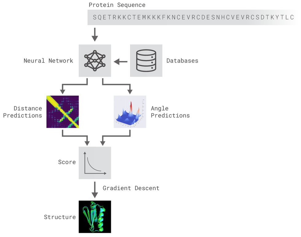
 5 | The methods implemented are inspired by DeepMind's original post. Two different residual neural networks (ResNets) are used to predict **angles** between adjacent aminoacids (AAs) and **distance** between every pair of AAs of a protein. For distance prediction a 2D Resnet was used while for angles prediction a 1D Resnet was used.
 6 | 
 7 | <div style="text-align:center">
 8 | 	<img src="https://storage.googleapis.com/deepmind-live-cms/images/Origami-CASP-181127-r01_fig4-method.width-980.png" width="600" height="400">
 9 | </div>
10 | 
11 | Image from DeepMind's original blogpost.
12 | 
13 | ### Distance prediction
14 | 
15 | The ResNet for distance prediction is built as a 2D-ResNet and takes as input tensors of shape LxLxN (a normal image would be LxLx3). The window length is set to 200 (we only train and predict proteins of less than 200 AAs) and smaller proteins are padded to match the window size. No larger proteins nor crops of larger proteins are used.
16 | 
17 | The 41 channels of the input are distributed as follows: 20 for AAs in one-hot encoding (LxLx20), 1 for the Van der Waals radius of the AA encoded previously and 20 channels for the Position Specific Scoring Matrix).
18 | 
19 | The network is comprised of packs of residual blocks with the architecture below illustrated with blocks cycling through 1,2,4 and 8 strides plus a first normal convolutional layer and the last convolutional layer where a Softmax activation function is applied to get an output of LxLx7 (6 classes for different distance + 1 trash class for the padding that is less penalized).
20 | 
21 | <div style="text-align:center">
22 | 	<img src="imgs/elu_resnet_2d.png">
23 | </div>
24 | 
25 | Architecture of the residual block used. A mini version of the block in [this description](http://predictioncenter.org/casp13/doc/presentations/Pred_CASP13-DeepLearning-AlphaFold-Senior.pdf)
26 | 
27 | The network has been trained with 134 proteins and evaluated with 16 more. Clearly unsufficient data, but memory constraints didn't allow for more. Comparably, AlphaFold was trained with 29k proteins.
28 | 
29 | The output of the network is, then, a classification among 6 classes wich are ranges of distances between a pair of AAs. Here there's an example of AlphaFold predicted distances and the distances predicted by our model:
30 | 
31 | <div style="text-align:center">
32 | 	<img src="imgs/alphafold_preds.png", width="600">
33 | </div>
34 | Ground truth (left) and predicted distances (right) by AlphaFold.
35 | 
36 | <div style="text-align:center">
37 | 	<img src="models/distance_pipeline/images/golden_img_v91_45.png", width="900">
38 | </div>
39 | Ground truth (left) and predicted distances (right) by MiniFold.
40 | 
41 | The architecture of the Residual Network for distance prediction is very simmilar, the main difference being that the model here described was trained with windows of 200x200 AAs while AlphaFold was trained with crops of 64x64 AAs. When it comes to prediction, AlphaFold used the smaller window size to average across different outputs and achieve a smoother result. Our prediction, however, is a unique window, so there's no average (noisier predictions).
42 | 
43 | 
44 | ### Angles prediction
45 | 
46 | The ResNet for angles prediction is built as a 1D-ResNet and takes as input tensors of shape LxN. The window length is set to 34 and we only train and predict aangles of proteins with less than 200 (L) AAs. No larger proteins nor crops of larger proteins are used.
47 | 
48 | The 42 (N) channels of the input are distributed as follows: 20 for AAs in one-hot encoding (Lx20), 2 for the Van der Waals radius and the surface accessibility of the AA encoded previously and 20 channels for the Position Specific Scoring Matrix).
49 | 
50 | We followed the ResNet20 architecture but replaced the 2D Convolutions by 1D convolutions. The network output consists of a vector of 4 numbers that represent the `sin` and `cos` of the 2 dihedral angles between two AAs (Phi and Psi).
51 | 
52 | Dihedral angles were extracted from raw coordinates of the protein backbone atoms (N-terminus, C-alpha and C-terminus of each AA). The plot of Phi and Psi recieves the name of Ramachandran plot: 
53 | 
54 | <div style="text-align:center">
55 | 	<img src="imgs/ramachandran_plot.png">
56 | </div>
57 | The cluster observed in the upper-left region corresponds to the angles comprised between AAs when they form a Beta-sheet while the cluster observed in the central-left region corresponds to the angles comprised between AAs when they form an Alpha-helix.
58 | 
59 | The results of the model when making predictions can be observed below:
60 | <div style="text-align:center">
61 | 	<img src="imgs/angle_preds.png">
62 | </div>
63 | 
64 | The network has been trained with crops 38,7k crops from 600 different proteins and evaluated with some 4,3k more.
65 | 
66 | The architecture of the Residual Network is different from the one implemented in AlphaFold. The model here implemented was inspired by [this paper](https://journals.plos.org/ploscompbiol/article?id=10.1371/journal.pcbi.1005324) and [this one](https://journals.plos.org/plosone/article?id=10.1371/journal.pone.0205819).
67 | 
68 | ## Results
69 | While the architectures implemented in this first preliminary version of the project are inspired by papers with great results, the results here obtained are not as good as they could be. It's probable that the lack of Multiple Alignmnent (MSA), MSA-based features, Physicochemichal properties of AAs (beyond Van der Waals radius) or the lack of both model and feature engineering have affected the models negatively, as well as the little data that they have been trained on. 
70 | 
71 | For that reason, we can conclude that it has been a somehow naive approach and we expect to further implement some ideas/improvements to these models. As the DeepMind team says: *"With few or no alignments accuracy is much worse"*. It would be interesting to use the predictions made by the models as constraints to a folding algorithm (ie. Rosetta) in order to visualize our results.
72 | 
73 | ## References
74 | * [DeepMind original blog post](https://deepmind.com/blog/alphafold/)
75 | * [AlphaFold @ CASP13: “What just happened?”](https://moalquraishi.wordpress.com/2018/12/09/alphafold-casp13-what-just-happened/#s2.2)
76 | * [Accurate De Novo Prediction of Protein Contact Map by Ultra-Deep Learning Model](https://journals.plos.org/ploscompbiol/article?id=10.1371/journal.pcbi.1005324)
77 | * [AlphaFold slides](http://predictioncenter.org/casp13/doc/presentations/Pred_CASP13-DeepLearning-AlphaFold-Senior.pdf)
78 | * [De novo protein structure prediction using ultra-fast molecular dynamics simulation](https://journals.plos.org/plosone/article?id=10.1371/journal.pone.0205819)
79 | 


--------------------------------------------------------------------------------
/models/angles/resnet_1d_angles.h5:
--------------------------------------------------------------------------------
https://raw.githubusercontent.com/hypnopump/MiniFold/6eb47c5600c22c7dabbb1294adbd8c6704a185cb/models/angles/resnet_1d_angles.h5


--------------------------------------------------------------------------------
/models/angles/resnet_1d_angles.py:
--------------------------------------------------------------------------------
  1 | # Import libraries
  2 | import keras
  3 | import keras.backend as K
  4 | from keras.models import Model
  5 | # Optimizer and regularization
  6 | from keras.regularizers import l2
  7 | from keras.losses import mean_squared_error, mean_absolute_error
  8 | # Keras layers
  9 | from keras.layers.convolutional import Conv1D
 10 | from keras.layers import Dense, Dropout, Flatten, Input, BatchNormalization, Activation
 11 | from keras.layers.pooling import MaxPooling1D, AveragePooling1D
 12 | 
 13 | 
 14 | def custom_mse_mae(y_true, y_pred):
 15 |     """ Custom loss function - MSE + MAE """
 16 |     return mean_squared_error(y_true, y_pred)+mean_absolute_error(y_true, y_pred)
 17 | 
 18 | def resnet_layer(inputs,
 19 |                  num_filters=16,
 20 |                  kernel_size=3,
 21 |                  strides=1,
 22 |                  activation='relu',
 23 |                  batch_normalization=True,
 24 |                  conv_first=False):
 25 |     """2D BN-Relu-Conv (ResNet preact structure) or Conv-BN-Relu stack builder
 26 | 
 27 |     # Arguments
 28 |         inputs (tensor): input tensor from input image or previous layer
 29 |         num_filters (int): Conv2D number of filters
 30 |         kernel_size (int): Conv2D square kernel dimensions
 31 |         strides (int): Conv2D square stride dimensions
 32 |         activation (string): activation name
 33 |         batch_normalization (bool): whether to include batch normalization
 34 |         conv_first (bool): conv-bn-activation (True) or
 35 |             bn-activation-conv (False)
 36 | 
 37 |     # Returns
 38 |         x (tensor): tensor as input to the next layer
 39 |     """
 40 |     conv = Conv1D(num_filters,
 41 |                   kernel_size=kernel_size,
 42 |                   strides=strides,
 43 |                   padding='same',
 44 |                   kernel_initializer='he_normal',
 45 |                   kernel_regularizer=l2(1e-4))
 46 | 
 47 |     x = inputs
 48 |     if conv_first:
 49 |         x = conv(x)
 50 |         if batch_normalization:
 51 |             x = BatchNormalization()(x)
 52 |         if activation is not None:
 53 |             x = Activation(activation)(x)
 54 |     else:
 55 |         if batch_normalization:
 56 |             x = BatchNormalization()(x)
 57 |         if activation is not None:
 58 |             x = Activation(activation)(x)
 59 |         x = conv(x)
 60 |     return x
 61 | 
 62 | def resnet_v2(input_shape, depth, num_classes=4, conv_first=True):
 63 |     """ResNet Version 2 Model builder [b]
 64 | 
 65 |     Stacks of (1 x 1)-(3 x 3)-(1 x 1) BN-ReLU-Conv2D or also known as
 66 |     bottleneck layer
 67 |     First shortcut connection per layer is 1 x 1 Conv2D.
 68 |     Second and onwards shortcut connection is identity.
 69 |     At the beginning of each stage, the feature map size is halved (downsampled)
 70 |     by a convolutional layer with strides=2, while the number of filter maps is
 71 |     doubled. Within each stage, the layers have the same number filters and the
 72 |     same filter map sizes.
 73 |     Features maps sizes:
 74 |     conv1  : 32,  16
 75 |     stage 0: 32,  64
 76 |     stage 1: 16, 128
 77 |     stage 2:  8,  256
 78 | 
 79 |     # Arguments
 80 |         input_shape (tensor): shape of input image tensor
 81 |         depth (int): number of core convolutional layers
 82 |         num_classes (int): number of classes (CIFAR10 has 10)
 83 | 
 84 |     # Returns
 85 |         model (Model): Keras model instance
 86 |     """
 87 |     if (depth - 2) % 9 != 0:
 88 |         raise ValueError('depth should be 9n+2 (eg 56 or 110 in [b])')
 89 |     # Start model definition.
 90 |     num_filters_in = 16
 91 |     num_res_blocks = int((depth - 2) / 9)
 92 | 
 93 |     inputs = Input(shape=input_shape)
 94 |     # v2 performs Conv1D with BN-ReLU on input before splitting into 2 paths
 95 |     x = resnet_layer(inputs=inputs,
 96 |                      num_filters=num_filters_in,
 97 |                      conv_first=True)
 98 | 
 99 |     # Instantiate the stack of residual units
100 |     for stage in range(3):
101 |         for res_block in range(num_res_blocks):
102 |             activation = 'relu'
103 |             batch_normalization = True
104 |             strides = 1
105 |             if stage == 0:
106 |                 num_filters_out = num_filters_in * 4
107 |                 if res_block == 0:  # first layer and first stage
108 |                     activation = None
109 |                     batch_normalization = False
110 |             else:
111 |                 num_filters_out = num_filters_in * 2
112 |                 if res_block == 0:  # first layer but not first stage
113 |                     strides = 2    # downsample
114 | 
115 |             # bottleneck residual unit
116 |             y = resnet_layer(inputs=x,
117 |                              num_filters=num_filters_in,
118 |                              kernel_size=1,
119 |                              strides=strides,
120 |                              activation=activation,
121 |                              batch_normalization=batch_normalization,
122 |                              conv_first=conv_first)
123 |             y = resnet_layer(inputs=y,
124 |                              num_filters=num_filters_in,
125 |                              conv_first=conv_first)
126 |             y = resnet_layer(inputs=y,
127 |                              num_filters=num_filters_out,
128 |                              kernel_size=1,
129 |                              conv_first=conv_first)
130 |             if res_block == 0:
131 |                 # linear projection residual shortcut connection to match
132 |                 # changed dims
133 |                 x = resnet_layer(inputs=x,
134 |                                  num_filters=num_filters_out,
135 |                                  kernel_size=1,
136 |                                  strides=strides,
137 |                                  activation=None,
138 |                                  batch_normalization=False)
139 |             x = keras.layers.add([x, y])
140 | 
141 |         num_filters_in = num_filters_out
142 | 
143 |     # Add classifier on top.
144 |     # v2 has BN-ReLU before Pooling
145 |     x = BatchNormalization()(x)
146 |     x = Activation('relu')(x)
147 |     x = AveragePooling1D(pool_size=3)(x)
148 |     y = Flatten()(x)    
149 |     outputs = Dense(num_classes,
150 |                     activation='linear',
151 |                     kernel_initializer='he_normal')(y)
152 | 
153 |     # Instantiate model.
154 |     model = Model(inputs=inputs, outputs=outputs)
155 |     return model
156 | 
157 | # Check it's working
158 | if __name__ == "__main__":
159 | 	# Using AMSGrad optimizer for speed 
160 | 	kernel_size, filters = 3, 16
161 | 	adam = keras.optimizers.Adam(amsgrad=True)
162 | 	# Create model
163 | 	model = resnet_v2(input_shape=(17*2,41), depth=20, num_classes=4)
164 | 	model.compile(optimizer=adam, loss=custom_mse_mae,
165 | 				  metrics=["mean_absolute_error", "mean_squared_error"])
166 | 	model.summary()
167 | 	print("Model file works perfectly")
168 | 


--------------------------------------------------------------------------------
/models/distance_pipeline/Tutorials/README.pdf:
--------------------------------------------------------------------------------
https://raw.githubusercontent.com/hypnopump/MiniFold/6eb47c5600c22c7dabbb1294adbd8c6704a185cb/models/distance_pipeline/Tutorials/README.pdf


--------------------------------------------------------------------------------
/models/distance_pipeline/Tutorials/RR_format.py:
--------------------------------------------------------------------------------
 1 | RR_FORMAT = """PFRMAT RR
 2 | MODEL 1
 3 | """
 4 | def save_rr(seq,sample_pred,file_name_rr):
 5 |   my_file=open(file_name_rr,'w')
 6 |   my_file.write(RR_FORMAT)
 7 |   my_file.write(seq + '\n')
 8 |   for i in range(0,len(seq)):
 9 |     for j in range(i+5,len(seq)):
10 |       print(max(sample_pred[0][i][j]))
11 |       my_file.write(str(i+1)+" "+ str(j+1)+" "+"0 8 "+ str(max(sample_pred[0][i][j]))+"\n")
12 |   my_file.write('END\n')
13 |   my_file.close()
14 | save_rr(seq,sample_pred,'file_name_rr')
15 | 


--------------------------------------------------------------------------------
/models/distance_pipeline/Tutorials/modify_pssm.py:
--------------------------------------------------------------------------------
 1 | with open("file_name.pssm", "r") as f:
 2 |     lines = f.readlines()[2:-6]
 3 | key  = "ACDEFGHIKLMNPQRSTVWY"
 4 | text_keys = lines[0].replace("\n", "").split("   ")[4:]
 5 | 
 6 | # PSSM OPTION 1
 7 | text_vals = np.array([" ".join(line.replace("\n", "")[72:-11].split()).split() for line in lines[1:]]).astype(float)
 8 | 
 9 | # PSSM OPTION 2
10 | # text_vals = np.array([" ".join(line.replace("\n", "")[10:72].split()).split() for line in lines[1:]]).astype(float)
11 | 
12 | # normalize to [0,1]
13 | # text_vals = text_vals / np.sum(text_vals, axis=1).reshape((len(text_vals), 1))
14 | for i in range(len(text_vals)):
15 |     text_vals[i] = (text_vals[i] - np.amin(text_vals[i])) / (np.amax(text_vals[i] - np.amin(text_vals[i])))
16 | 
17 | # create NxL PSSM
18 | pssm      = np.zeros_like(text_vals)
19 | for i,aa in enumerate(text_keys):
20 |     pssm[key.index(aa), :] = text_vals[i, :] 
21 |     
22 | inputs_pssm = wider_pssm(pssm.T, seq)
23 | inputs = np.concatenate((inputs_aa, inputs_pssm), axis=-1)
24 | 


--------------------------------------------------------------------------------
/models/distance_pipeline/distance_generator_data.py:
--------------------------------------------------------------------------------
  1 | import keras
  2 | import numpy as np
  3 | # Custom functions import
  4 | from func_utils import *
  5 | 
  6 | class DataGenerator(keras.utils.Sequence):
  7 |     'Generates data for Keras'
  8 |     def __init__(self, paths=None, max_prots=10, batch_size=8, crop_size=200, pad_size=200,
  9 |                  n_classes=5, class_cuts=[-0.5, 500, 1000, 1700], shuffle=True):
 10 |         'Initialization'
 11 |         # Get data
 12 |         self.names, self.seqs, self.dists, self.pssms = get_data(paths, max_prots)
 13 |         self.list_IDs = [i for i in range(len(self.seqs))]
 14 |         # Features
 15 |         self.batch_size = batch_size
 16 |         self.crop_size = crop_size
 17 |         self.pad_size = pad_size
 18 |         self.n_classes = n_classes
 19 |         self.class_cuts = class_cuts
 20 |         if len(self.class_cuts) != self.n_classes-1:
 21 |             raise ValueError('len(class_cuts) must be n_classes-1')
 22 | 
 23 |         self.shuffle = shuffle
 24 |         self.on_epoch_end()
 25 | 
 26 |     def __len__(self):
 27 |         'Denotes the number of batches per epoch'
 28 |         return int(np.floor(len(self.list_IDs) / self.batch_size))
 29 | 
 30 |     def __getitem__(self, index):
 31 |         'Generate one batch of data'
 32 |         # Generate indexes of the batch
 33 |         indexes = self.indexes[index*self.batch_size:(index+1)*self.batch_size]
 34 | 
 35 |         # Find list of IDs
 36 |         list_IDs_temp = [self.list_IDs[k] for k in indexes]
 37 | 
 38 |         # Generate data
 39 |         x, y = self.__data_generation(list_IDs_temp)
 40 | 
 41 |         return x, y
 42 | 
 43 |     def get_data(self, paths, max_prots):
 44 |         """ Get the data from files. """
 45 |         # Scan first n proteins
 46 |         names = []
 47 |         seqs = []
 48 |         dists = []
 49 |         pssms = []
 50 |         for path in paths: 
 51 |             # Opn file and read text
 52 |             with open(path, "r") as f:
 53 |                 lines = f.read().split('\n')
 54 | 
 55 |             # Extract numeric data from text
 56 |             for i,line in enumerate(lines):
 57 |                 if len(names) == max_prots+1:
 58 |                     break
 59 |                 # Read each protein separately
 60 |                 if line == "[ID]":
 61 |                     names.append(lines[i+1])
 62 |                 elif line == "[PRIMARY]":
 63 |                     seqs.append(lines[i+1])
 64 |                 elif line == "[EVOLUTIONARY]":
 65 |                     pssms.append(parse_lines(lines[i+1:i+21]))
 66 |                 elif line == "[DIST]":
 67 |                     dists.append(parse_lines(lines[i+1:i+len(seqs[-1])+1]))
 68 |                     # Progress control
 69 |                     if len(names)%100 == 0:
 70 |                         print("Currently @ ", len(names), " out of "+str(max_prots))
 71 |                         try: logger.info("Currently @ ", len(names), " out of "+str(max_prots))
 72 |                         except:pass
 73 | 
 74 |         print("Total length is "+str(len(names)-1)+" out of "+str(max_prots)+" possible.")
 75 |         try: logger.info("Total length is "+str(len(names)-1)+" out of "+str(max_prots)+" possible.")
 76 |         except:pass
 77 | 
 78 |         return names, seqs, dists, pssms
 79 | 
 80 | 
 81 |     def on_epoch_end(self):
 82 |         'Updates indexes after each epoch'
 83 |         self.indexes = np.arange(len(self.list_IDs))
 84 |         if self.shuffle == True:
 85 |             np.random.shuffle(self.indexes)
 86 |                                                      
 87 |     def wider(self, seq, n=20):
 88 |         """ Converts a seq into a one-hot tensor. Not LxN but LxLxN"""
 89 |         key = "HRKDENQSYTCPAVLIGFWM"
 90 |         tensor = []
 91 |         for i in range(self.pad_size):
 92 |             d2 = []
 93 |             for j in range(self.pad_size):
 94 |                 # Check first for lengths (dont want index_out_of_range)
 95 |                 d1 = [1 if (j<len(seq) and i<len(seq) and key[x] == seq[i] and key[x] == seq[j])
 96 |                       else 0 for x in range(n)]
 97 | 
 98 |                 d2.append(d1)
 99 |             tensor.append(d2)
100 | 
101 |         return np.array(tensor)
102 |                                                      
103 |     def wider_pssm(self, pssm, seq, n=20):
104 |         """ Converts a seq into a tensor. Not LxN but LxLxN.
105 |             Multiply cell i,j x j,i to create an LxLxN tensor.
106 |         """
107 |         key = "HRKDENQSYTCPAVLIGFWM"
108 |         key_alpha = "ACDEFGHIKLMNPQRSTVWY"
109 |         tensor = []
110 |         for i in range(self.pad_size):
111 |             d2 = []
112 |             for j in range(self.pad_size):
113 |                 # Check first for lengths (dont want index_out_of_range)
114 |                 if j<len(seq) and i<len(seq):
115 |                     d1 = [aa[i]*aa[j] for aa in pssm]
116 |                 else:
117 |                     d1 = [0 for i in range(n)]
118 | 
119 |                 # Append pssm[i]*pssm[j]
120 |                 if j<len(seq) and i<len(seq):
121 |                     d1.append(pssm[key_alpha.index(seq[i])][i] *
122 |                               pssm[key_alpha.index(seq[j])][j])
123 |                 else: 
124 |                     d1.append(0)
125 |                 # Append manhattan distance to diagonal but reversed (center=0, xtremes=1)
126 |                 d1.append(1 - abs(i-j)/self.crop_size)
127 | 
128 |                 d2.append(d1)
129 |             tensor.append(d2)
130 | 
131 |         return np.array(tensor)
132 |                                                      
133 |     def treshold(self, matrix):
134 |         """ Turns an L*L*1 tensor into an L*L*N """
135 |         med = []
136 |         # Create labels for classes
137 |         for i,cat in enumerate(self.class_cuts):
138 |             if i < self.n_classes-1:
139 |                 inter = (np.array(matrix)<self.class_cuts[i]).astype(np.int)
140 |                 # Subtract all previous (don't do it for first one)
141 |                 if i != 0: 
142 |                     for prev in med: 
143 |                         inter -= prev
144 | 
145 |             med.append(inter)
146 | 
147 |         # Append last class (greater than lass class_cut)
148 |         med.append((np.array(matrix)>=self.class_cuts[-1]).astype(np.int))
149 | 
150 |         return np.concatenate([cat.reshape(self.pad_size, self.pad_size, 1) 
151 |                                for cat in med], axis=2)
152 |                                                      
153 |     # Embed number of rows
154 |     def embedding_matrix(self, matrix):
155 |         # Embed with extra columns
156 |         for i in range(len(matrix)):
157 |             while len(matrix[i])<self.pad_size:
158 |                 matrix[i].extend([-1 for i in range(self.pad_size-len(matrix[i]))])
159 |         #Embed with extra rows
160 |         while len(matrix)<self.pad_size:
161 |             matrix.append([-1 for x in range(self.pad_size)])
162 |         return np.array(matrix)
163 | 
164 |     # Get indices to crop from a splice of (crop_size x crop_size)
165 |     def random_indices(self, list_IDs_temp):
166 |         indices = []
167 |         for i in list_IDs_temp:
168 |             if len(self.seqs[i])<=self.crop_size:
169 |                 indices.append([0,0])
170 |             else:
171 |                 indices.append([np.random.randint(0, len(self.seqs[i])-self.crop_size),
172 |                                 np.random.randint(0, len(self.seqs[i])-self.crop_size)])
173 |         return indices
174 | 
175 |     def __data_generation(self, list_IDs_temp):
176 |         'Generates data containing batch_size samples' # X : (n_samples, *dim, n_channels)
177 |         # Initialization
178 |         # Get the random indices to crop from
179 |         r_i = self.random_indices(list_IDs_temp) 
180 |         # Get data
181 |         inputs_aa = np.array([self.wider(self.seqs[i])[r_i[k][0]:r_i[k][0]+self.crop_size, r_i[k][1]:r_i[k][1]+self.crop_size]
182 |                               for k,i in enumerate(list_IDs_temp)])
183 |         inputs_pssm = np.array([self.wider_pssm(self.pssms[i], self.seqs[i])[r_i[k][0]:r_i[k][0]+self.crop_size, r_i[k][1]:r_i[k][1]+self.crop_size]
184 |                                 for k,i in enumerate(list_IDs_temp)])
185 |         # print(self.inputs_aa.shape, self.inputs_pssm.shape)
186 |         x = np.concatenate((inputs_aa, inputs_pssm), axis=3)
187 |         # Get labels
188 |         distas = np.array([self.embedding_matrix(self.dists[i]) for i in list_IDs_temp])                      
189 |         y = np.array([self.treshold(d)[r_i[k][0]:r_i[k][0]+self.crop_size, r_i[k][1]:r_i[k][1]+self.crop_size]
190 |                       for k,d in enumerate(distas)])
191 |         
192 |         # try to free some memory
193 |         del inputs_aa
194 |         del inputs_pssm
195 |         del distas
196 |         del r_i
197 | 
198 |         return x,y


--------------------------------------------------------------------------------
/models/distance_pipeline/elu_resnet_2d_distances.py:
--------------------------------------------------------------------------------
  1 | # Import libraries
  2 | import numpy as np
  3 | import keras
  4 | import keras.backend as K
  5 | from keras.models import Model
  6 | # Activation and Regularization
  7 | from keras.regularizers import l2
  8 | from keras.activations import softmax
  9 | # Keras layers
 10 | from keras.layers.convolutional import Conv2D, Conv2DTranspose
 11 | from keras.layers import Dense, Dropout, Flatten, Input, BatchNormalization, Activation
 12 | from keras.layers.pooling import MaxPooling2D, AveragePooling2D
 13 | 
 14 | 
 15 | def softMaxAxis2(x):
 16 |     """ Compute softmax on axis 2. """
 17 |     return softmax(x,axis=2)
 18 | 
 19 | 
 20 | def weighted_categorical_crossentropy(weights):
 21 |     """
 22 |     A weighted version of keras.objectives.categorical_crossentropy
 23 |     
 24 |     Variables:
 25 |         weights: numpy array of shape (C,) where C is the number of classes
 26 |     
 27 |     Usage:
 28 |         weights = np.array([0.5,2,10]) # Class one at 0.5, class 2 twice the normal weights, class 3 10x.
 29 |         loss = weighted_categorical_crossentropy(weights)
 30 |         model.compile(loss=loss,optimizer='adam')
 31 |     """
 32 |     
 33 |     weights = K.variable(weights)
 34 |         
 35 |     def loss(y_true, y_pred):
 36 |         # scale predictions so that the class probas of each sample sum to 1
 37 |         y_pred /= K.sum(y_pred, axis=-1, keepdims=True)
 38 |         # clip to prevent NaN's and Inf's
 39 |         y_pred = K.clip(y_pred, K.epsilon(), 1 - K.epsilon())
 40 |         # calc
 41 |         loss = y_true * K.log(y_pred) * weights
 42 |         loss = -K.sum(loss, -1)
 43 |         return loss
 44 |     
 45 |     return loss
 46 | 
 47 | 
 48 | def resnet_block(inputs,
 49 |                  num_filters=64,
 50 |                  kernel_size=3,
 51 |                  strides=1,
 52 |                  activation='elu',
 53 |                  batch_normalization=True,
 54 |                  conv_first=False):
 55 |     """ # Arguments
 56 |         inputs (tensor): input tensor from input image or previous layer
 57 |         num_filters (int): Conv2D number of filters
 58 |         kernel_size (int): Conv2D square kernel dimensions
 59 |         strides (int): Conv2D square stride dimensions
 60 |         activation (string): activation name
 61 |         batch_normalization (bool): whether to include batch normalization
 62 |         conv_first (bool): conv-bn-activation (True) or
 63 |             bn-activation-conv (False)
 64 |     """
 65 | 
 66 |     x = inputs
 67 |     # down size
 68 |     x = BatchNormalization()(x)
 69 |     x = Activation(activation)(x)
 70 |     x = Conv2D(num_filters//2, kernel_size=1, strides=1, padding='same',
 71 |                kernel_initializer='he_normal', kernel_regularizer=l2(1e-4))(x)
 72 |     # Strided Calculations - cyclic strides - half filters
 73 |     x = BatchNormalization()(x)
 74 |     x = Activation(activation)(x)
 75 |     x = Conv2D(num_filters//2, kernel_size=3, strides=strides, padding='same',
 76 |                kernel_initializer='he_normal', kernel_regularizer=l2(1e-4))(x)
 77 |     # Up size
 78 |     x = BatchNormalization()(x)
 79 |     x = Activation(activation)(x)
 80 |     x = Conv2DTranspose(num_filters, kernel_size=1, strides=strides, padding='same',
 81 |                         kernel_initializer='he_normal', kernel_regularizer=l2(1e-4))(x)
 82 |     return x
 83 | 
 84 | 
 85 | def resnet_layer(inputs,
 86 |                  num_filters=32,
 87 |                  kernel_size=3,
 88 |                  strides=1,
 89 |                  activation='relu',
 90 |                  batch_normalization=True,
 91 |                  conv_first=False):
 92 |     """2D Convolution-Batch Normalization-Activation stack builder
 93 | 
 94 |     # Arguments
 95 |         inputs (tensor): input tensor from input image or previous layer
 96 |         num_filters (int): Conv2D number of filters
 97 |         kernel_size (int): Conv2D square kernel dimensions
 98 |         strides (int): Conv2D square stride dimensions
 99 |         activation (string): activation name
100 |         batch_normalization (bool): whether to include batch normalization
101 |         conv_first (bool): conv-bn-activation (True) or
102 |             bn-activation-conv (False)
103 | 
104 |     # Returns
105 |         x (tensor): tensor as input to the next layer
106 |     """
107 |     conv = Conv2D(num_filters,
108 |                   kernel_size=kernel_size,
109 |                   strides=strides,
110 |                   padding='same',
111 |                   kernel_initializer='he_normal',
112 |                   kernel_regularizer=l2(1e-4))
113 | 
114 |     x = inputs
115 |     if conv_first:
116 |         x = conv(x)
117 |         if batch_normalization:
118 |             x = BatchNormalization()(x)
119 |         if activation is not None:
120 |             x = Activation(activation)(x)
121 |     else:
122 |         if batch_normalization:
123 |             x = BatchNormalization()(x)
124 |         if activation is not None:
125 |             x = Activation(activation)(x)
126 |         x = conv(x)
127 |     return x
128 | 
129 | 
130 | def resnet_v2(input_shape, depth, num_classes=4):
131 |     """ Elu ResNet Model builder.
132 |         * depth should be multiple of 4
133 |     """
134 |     if depth % 4 != 0:
135 |         raise ValueError('depth should be 4n (eg 8 or 16)')
136 |     # Start model definition.
137 |     num_filters_in = 64
138 |     inputs = Input(shape=input_shape)
139 |     # v2 performs Conv2D with BN-ReLU on input before splitting into 2 paths
140 |     x = resnet_layer(inputs=inputs,
141 |                      num_filters=num_filters_in,
142 |                      conv_first=True)
143 | 
144 |     # Instantiate the stack of residual units
145 |     striding = [1,2,4,8]
146 |     for stage in range(depth):
147 | 
148 |         activation = 'elu'
149 |         batch_normalization = True
150 | 
151 |         # bottleneck residual unit
152 |         y = resnet_block(inputs=x,
153 |                          num_filters=64,
154 |                          kernel_size=3,
155 |                          strides=striding[stage%4])
156 | 
157 |         x = keras.layers.add([x, y])
158 | 
159 |     # Add a linear Conv classifier on top.
160 |     # v2 has BN-ReLU before Pooling
161 |     y = Conv2D(num_classes, kernel_size=1, strides=1, padding='same',
162 |     	       kernel_initializer='he_normal', kernel_regularizer=l2(1e-4))(x)
163 |     outputs = Activation(softMaxAxis2)(y)
164 | 
165 |     # Instantiate model.
166 |     model = Model(inputs=inputs, outputs=outputs)
167 |     return model
168 | 
169 | 
170 | # Check it's working
171 | if __name__ == "__main__":
172 |     # Using AMSGrad optimizer for speed 
173 |     kernel_size, filters = 3, 16
174 |     adam = keras.optimizers.Adam(amsgrad=True)
175 |     # Create model
176 |     model = model = resnet_v2(input_shape=(200,200, 40), depth=8, num_classes=7)
177 |     model.compile(optimizer=adam, loss=weighted_categorical_crossentropy(
178 |                   np.array([0.01,1,0.9,0.8,0.7,0.6,0.5])), metrics=["accuracy"])
179 |     model.summary()
180 |     print("Model file works perfectly")
181 | 


--------------------------------------------------------------------------------
/models/distance_pipeline/evaluation_pipeline.py:
--------------------------------------------------------------------------------
  1 | # Import libraries
  2 | import numpy as np
  3 | import matplotlib.pyplot as plt
  4 | # Import libraries
  5 | import keras
  6 | import keras.backend as K
  7 | from keras.models import Model, load_model, Sequential
  8 | # Activation and Regularization
  9 | from keras.regularizers import l2
 10 | from keras.activations import softmax
 11 | # Keras layers
 12 | from keras.layers.convolutional import Conv2D, Conv2DTranspose
 13 | from keras.layers import Dense, Dropout, Flatten, Input, BatchNormalization, Activation
 14 | from keras.layers.pooling import MaxPooling2D, AveragePooling2D
 15 | 
 16 | # Model architecture
 17 | from elu_resnet_2d_distances import *
 18 | from func_utils import *
 19 | # Logs-related imports
 20 | import sys
 21 | import logging
 22 | import os
 23 | 
 24 | 
 25 | # Log progress
 26 | logger.info("Gonna evaluate the model")
 27 | logger.info("Loading data")
 28 | 
 29 | path = "../../data/distanced/full_under_200.txt"
 30 | # Opn file and read text
 31 | with open(path, "r") as f:
 32 | 	lines = f.read().split('\n')
 33 | 
 34 | # Scan first n proteins
 35 | names, seqs, dists, pssms = get_data(paths=[EVAL_SOURCE_PATH], max_prots=MAX_PROTS_EVAL)
 36 | 
 37 | # preprocess inputs
 38 | inputs_aa = np.array([wider(seq) for seq in seqs])
 39 | inputs_aa.shape
 40 | inputs_pssm = np.array([wider_pssm(pssms[i], seqs[i]) for i in range(len(pssms))])
 41 | inputs_pssm.shape
 42 | inputs = np.concatenate((inputs_aa, inputs_pssm), axis=3)
 43 | print(inputs.shape)
 44 | # Delete unnecessary data
 45 | del inputs_pssm
 46 | del inputs_aa
 47 | dists = np.array([embedding_matrix(matrix) for matrix in dists])
 48 | outputs = np.array([treshold(d, CLASS_CUTS) for d in dists])
 49 | print(outputs.shape)
 50 | del dists
 51 | 
 52 | # Log progress
 53 | logger.info("Data loaded correctly")
 54 | logger.info("Load the model")
 55 | 
 56 | # Set WEIGHTS
 57 | print("WEIGHTS", WEIGHTS)
 58 |  
 59 | # Load model
 60 | model = load_model(STAGE_MODEL_PATH,
 61 | 			custom_objects={'loss': weighted_categorical_crossentropy(np.array(WEIGHTS)),
 62 | 			'softMaxAxis2': softMaxAxis2})	
 63 | model.compile(optimizer=adam,
 64 | 			  loss=weighted_categorical_crossentropy(np.array(WEIGHTS)),
 65 | 			  metrics=["accuracy"])
 66 | 
 67 | # Log progress
 68 | logger.info("Model loaded")
 69 | logger.info("Let's predict")
 70 | 
 71 | # Predict and benchmark
 72 | i,k = 0, MAX_PROTS_PREDICT
 73 | sample_pred = model.predict([inputs[i:i+k]])
 74 | preds4 = np.argmax(sample_pred, axis=3)
 75 | preds4[preds4==0] = 6 # Change trash class by class for long distance
 76 | outs4 = np.argmax(outputs[i:i+k], axis=3)
 77 | outs4[outs4==0] = 6 # Change trash class by class for long distance
 78 | # Select the best prediction to display it - (proportional by protein length(area of contact map))
 79 | results = [np.sum(np.equal(pred[:len(seqs[i+j]), :len(seqs[i+j])], outs4[j, :len(seqs[i+j]), :len(seqs[i+j]),]),axis=(0,1))/
 80 | 			len(seqs[i+j])**2 
 81 | 			for j,pred in enumerate(preds4)]
 82 | best_score = max(results)
 83 | print("Best score (Accuracy): ", best_score)
 84 | sorted_scores = [acc for acc in sorted(results, key=lambda x: x, reverse=True)]
 85 | print("Best 5 scores: ", sorted_scores[:5])
 86 | sorted_indices = [results.index(x) for x in sorted_scores]
 87 | print("Best 5 indices: ", sorted_indices[:5])
 88 | 
 89 | # Log results: 
 90 | logger.info("Best 10 scores: "+str(sorted_scores[:10]))
 91 | logger.info("Best 10 indices: "+str(sorted_indices[:10]))
 92 | 
 93 | 
 94 | # Measure metrics and decide if model is better!
 95 | preds_crop = np.concatenate( [pred[:len(seqs[i+j]), :len(seqs[i+j])].flatten() for j,pred in enumerate(preds4)] )
 96 | outs_crop = np.concatenate( [outs4[j, :len(seqs[i+j]), :len(seqs[i+j])].flatten() for j,pred in enumerate(preds4)] )
 97 | 
 98 | total_mse = np.linalg.norm(outs_crop-preds_crop)
 99 | mse_prot = np.linalg.norm(outs_crop-preds_crop)/len(preds4)
100 | 
101 | print("Introducing total mse: ", total_mse)
102 | print("Introducing mse/prot: ", mse_prot)
103 | logger.info("total_mse: "+str(total_mse))
104 | logger.info("mse/prots: "+str(mse_prot))
105 | 
106 | # loading previous record. If not, make sure this one gets written.
107 | try: 
108 | 	with open(RECORD_PATH, "r") as f:
109 | 		lines = f.read().split('\n')
110 | 
111 | 	prev_total_mse = float(lines[0].split(" ")[-1])
112 | 	prev_mse_prot = float(lines[1].split(" ")[-1])
113 | except: 
114 | 	prev_total_mse = 1e8
115 | 	prev_mse_prot = 1e8
116 | 
117 | # compare metrics
118 | if total_mse < prev_total_mse and mse_prot < prev_mse_prot:
119 | 	print("model is better. saving. prev mse/prot: "+str(prev_mse_prot)+" new: "+str(mse_prot))
120 | 	logger.info("model is better. saving. prev mse/prot: "+str(prev_mse_prot)+" new: "+str(mse_prot))
121 | 	# save model and new records
122 | 	model.save(GOLDEN_MODEL_PATH)
123 | 	with open(RECORD_PATH, "w") as f:
124 | 		f.write("total_mse: "+str(total_mse)+"\n")
125 | 		f.write("mse/prot: "+str(mse_prot)+"\n")
126 | 		# Load WEIGHTS set that produced best outcome till now
127 | 		f.write(str(sys.argv[2])+" : "+str(sys.argv[3]))
128 | 	print("model saved. Producing images")
129 | 	logger.info("model saved.  Producing images")
130 | 
131 | 	# Avoid matplotlib logs
132 | 	logger.setLevel(40)
133 | 	# Make images 
134 | 	for best_score_index in sorted_indices[:3]+[i for i in range(10)]:
135 | 		plt.figure(figsize=(20,5))
136 | 		# First plot Ground Truth
137 | 		plt.subplot(1, 3, 1)
138 | 		plt.title('Ground Truth')
139 | 		plt.imshow(outs4[best_score_index, :len(seqs[i+best_score_index]), :len(seqs[i+best_score_index])],
140 | 					cmap='viridis_r', interpolation='nearest')
141 | 		plt.colorbar()
142 | 		plt.clim(0, N_CLASSES-1)
143 | 		# Then plot predictions by the mode
144 | 		plt.subplot(1, 3, 2)
145 | 		plt.title("Prediction by model")
146 | 		plt.imshow(preds4[best_score_index, :len(seqs[i+best_score_index]), :len(seqs[i+best_score_index])],
147 | 				cmap='viridis_r', interpolation='nearest')
148 | 		plt.colorbar()
149 | 		plt.clim(0, N_CLASSES-1)
150 | 		# Prediction by model (diag mirrored)
151 | 		plt.subplot(1, 3, 3)
152 | 		plt.title("Prediction by model - mirrored+averaged")
153 | 		plt.imshow(mirror_diag(preds4[best_score_index, :len(seqs[i+best_score_index]), :len(seqs[i+best_score_index])]),
154 | 					cmap='viridis_r', interpolation='nearest')
155 | 		plt.colorbar()
156 | 		plt.clim(0, N_CLASSES-1)
157 | 		# Show/Save them
158 | 		plt.savefig(IMAGES_PATH+str(best_score_index)+".png")
159 | 		# plt.show()
160 | 
161 | 	# Avoid matplotlib logs
162 | 	logger.setLevel(10)
163 | 	print("Images are ready")
164 | 	logger.info("Images are ready")
165 | else: 
166 | 	print("Model is no better than previous one. Not saving")  	
167 | 	logger.info("Model is no better than previous one. Not saving")
168 | 
169 | print("Evaluation finished")
170 | logger.info("Evaluation finished")
171 | logger.setLevel(40) 


--------------------------------------------------------------------------------
/models/distance_pipeline/func_utils.py:
--------------------------------------------------------------------------------
  1 | """ File to store functions (DRY) and params that are repeated
  2 |     Store config only in one site
  3 | """
  4 | import numpy as np 
  5 | import keras
  6 | # Logs-related imports
  7 | import sys
  8 | import logging
  9 | import os
 10 | 
 11 | # Logging info: - For reproducibility // 
 12 | # np.random.seed(5)
 13 | 
 14 | # PATHS
 15 | log_name = str(sys.argv[1])
 16 | LOG_PATH = str(os.getcwd())+"/"+log_name+".txt"
 17 | RECORD_PATH = "record.txt"
 18 | BASE_MODEL_PATH = "models/tester_28_lxl.h5"
 19 | STAGE_MODEL_PATH = "models/tester_28_lxl_stage.h5"
 20 | GOLDEN_MODEL_PATH = "models/tester_28_lxl_golden.h5"
 21 | IMAGES_PATH = "images/golden_img_v"+str(sys.argv[2])+"_"
 22 | TRAINING_PATHS = ["../../data/distanced/90_full_under_200.txt"] 
 23 |                 # "../data/distanced/70_full_under_200.txt"]
 24 | EVAL_SOURCE_PATH = "../../data/distanced/full_under_200.txt"
 25 | 
 26 | # PARAMS - DEFINE MODEL PARAMS
 27 | CROP_SIZE = 200                                      # Crops to feed the mmodel   
 28 | PAD_SIZE = 200                                       # Maximum length of any protein
 29 | CLASS_CUTS = [-0.5, 500, 750, 1000, 1400, 1700] # , 2000 # Cuts between classes 
 30 | N_CLASSES = len(CLASS_CUTS)+1                        # Number of classes
 31 | BATCH_SIZE = 2                                       # Size of each batch
 32 | MAX_PROTS = 1500 # 3500                              # Max number of prots in the dataset
 33 | BATCH_RATIO = 0.1 # Proportion of batches/prots (don't train on whole dataset)
 34 | print(str(sys.argv[3]).split(","))
 35 | WEIGHTS = [float(w) for w in str(sys.argv[3]).split(",")] # Class weights for the model
 36 | 
 37 | # EVAL PARAMS
 38 | MAX_PROTS_EVAL = 130
 39 | MAX_PROTS_PREDICT = 125 # 125
 40 | 
 41 | 
 42 | # Record settings
 43 | # LOG_FORMAT = "%(levelname)s %(asctime)s - %(message)s"
 44 | LOG_FORMAT = "%(asctime)s - %(message)s"
 45 | logging.basicConfig(filename=LOG_PATH,
 46 |                     format = LOG_FORMAT,
 47 |                     level = logging.DEBUG,
 48 |                     filemode = "a")
 49 | logger = logging.getLogger()
 50 | 
 51 | 
 52 | # Model-related variables 
 53 | kernel_size, filters = 3, 16
 54 | adam = keras.optimizers.Adam(lr=0.001, beta_1=0.9, beta_2=0.999, epsilon=None, decay=0.0, amsgrad=True)
 55 | 
 56 | 
 57 | # FUNC_UTILS
 58 | def parse_lines(raw):
 59 |     return [[float(x) for x in line.split("\t") if x != ""] for line in raw]
 60 | 
 61 | def parse_line(line):
 62 |     return [float(x) for x in line.split("\t") if x != ""]
 63 | 
 64 | 
 65 | def get_data(paths, max_prots):
 66 |         """ Get the data from files. """
 67 |         # Scan first n proteins
 68 |         names, seqs, dists, pssms = [], [], [], [] 
 69 | 
 70 |         for path in paths: 
 71 |             # Opn file and read text
 72 |             with open(path, "r") as f:
 73 |                 lines = f.read().split('\n')
 74 | 
 75 |             # Extract numeric data from text
 76 |             for i,line in enumerate(lines):
 77 |                 if len(names) == max_prots+1:
 78 |                     break
 79 |                 # Read each protein separately
 80 |                 if line == "[ID]":
 81 |                     names.append(lines[i+1])
 82 |                 elif line == "[PRIMARY]":
 83 |                     seqs.append(lines[i+1])
 84 |                 elif line == "[EVOLUTIONARY]":
 85 |                     pssms.append(parse_lines(lines[i+1:i+21]))
 86 |                 elif line == "[DIST]":
 87 |                     dists.append(parse_lines(lines[i+1:i+len(seqs[-1])+1]))
 88 |                     # Progress control
 89 |                     if len(names)%150 == 0:
 90 |                         print("Currently @ ", len(names), " out of "+str(max_prots))
 91 |                         try: logger.info("Currently @ "+str(len(names))+" out of "+str(max_prots))
 92 |                         except:pass
 93 | 
 94 |         print("Total length is "+str(len(names)-1)+" out of "+str(max_prots)+" possible.")
 95 |         try: logger.info("Total length is "+str(len(names)-1)+" out of "+str(max_prots)+" possible.")
 96 |         except:pass
 97 | 
 98 |         return names, seqs, dists, pssms
 99 | 
100 | 
101 | def wider(seq, l=200, n=20):
102 |     """ Converts a seq into a one-hot tensor. Not LxN but LxLxN"""
103 |     key = "HRKDENQSYTCPAVLIGFWM"
104 |     tensor = []
105 |     for i in range(l):
106 |         d2 = []
107 |         for j in range(l):
108 |             d1 = [1 if (j<len(seq) and i<len(seq) and key[x] == seq[i] and key[x] == seq[j]) else 0 for x in range(n)]
109 |     
110 |             d2.append(d1)
111 |         tensor.append(d2)
112 |     
113 |     return np.array(tensor)
114 | 
115 | 
116 | def wider_pssm(pssm, seq, l=200, n=20):
117 |     """ Converts a seq into a one-hot tensor. Not LxN but LxLxN"""
118 |     key = "HRKDENQSYTCPAVLIGFWM"
119 |     key_alpha = "ACDEFGHIKLMNPQRSTVWY"
120 |     tensor = []
121 |     for i in range(l):
122 |         d2 = []
123 |         for j in range(l):
124 |             if j<len(seq) and i<len(seq):
125 |                 d1 = [aa[i]*aa[j] for aa in pssm]
126 |             else:
127 |                 d1 = [0 for i in range(n)]
128 |                 
129 |             # Append pssm[i]*pssm[j]
130 |             if j<len(seq) and i<len(seq):
131 |                 d1.append(pssm[key_alpha.index(seq[i])][i] *
132 |                           pssm[key_alpha.index(seq[j])][j])
133 |             else: 
134 |                 d1.append(0)
135 |             # Append custom distance to diagonal formula (1-abs(i-j))/crop_size
136 |             # Works bad when i,j > len(seq)
137 |             d1.append(1 - abs(i-j)/200)
138 |     
139 |             d2.append(d1)
140 |         tensor.append(d2)
141 |     
142 |     return np.array(tensor)
143 | 
144 | 
145 | def embedding_matrix(matrix, l=200):
146 |     """ Embeds matrix of nxn into lxl. n<L """
147 |     # Embed with extra columns
148 |     for i in range(len(matrix)):
149 |         while len(matrix[i])<l:
150 |             matrix[i].extend([-1 for i in range(l-len(matrix[i]))])
151 |     #Embed with extra rows
152 |     while len(matrix)<l:
153 |         matrix.append([-1 for x in range(l)])
154 |     return np.array(matrix)
155 | 
156 | 
157 | def treshold(matrix, cuts=None, l=200): 
158 |     # Turns an L*L*1 tensor into an L*L*N 
159 |     trash = (np.array(matrix)<cuts[0]).astype(np.int)
160 |     first = (np.array(matrix)<cuts[1]).astype(np.int)-trash
161 |     sec = (np.array(matrix)<cuts[2]).astype(np.int)-trash-first
162 |     third = (np.array(matrix)<cuts[3]).astype(np.int)-trash-first-sec
163 |     fourth = (np.array(matrix)<cuts[4]).astype(np.int)-trash-first-sec-third
164 |     fifth = (np.array(matrix)<cuts[5]).astype(np.int)-trash-first-sec-third-fourth
165 | #     sixth = (np.array(matrix)<cuts[6]).astype(np.int)-trash-first-sec-third-fourth-fifth
166 |     seventh = np.array(matrix)>=cuts[5]
167 | 
168 |     return np.concatenate((trash.reshape(l,l,1),
169 |                            first.reshape(l,l,1),
170 |                            sec.reshape(l,l,1),
171 |                            third.reshape(l,l,1),
172 |                            fourth.reshape(l,l,1),
173 |                            fifth.reshape(l,l,1),
174 |                            # sixth.reshape(l,l,1),
175 |                            seventh.reshape(l,l,1)),axis=2)
176 | 
177 | def mirror_diag(image):
178 |     """ Mirrors image across its diagonal. """
179 |     image = image.astype(float)
180 |     # averages image across diagonal and returns 2 simetric parts
181 |     for i in range(len(image)):
182 |         for j in range(len(image[i])):
183 |             image[i,j] = image[j,i] = np.true_divide((image[i,j]+image[j,i]), 2)
184 |          
185 |     return image


--------------------------------------------------------------------------------
/models/distance_pipeline/images/FM_T0869_CASP12.jpg:
--------------------------------------------------------------------------------
https://raw.githubusercontent.com/hypnopump/MiniFold/6eb47c5600c22c7dabbb1294adbd8c6704a185cb/models/distance_pipeline/images/FM_T0869_CASP12.jpg


--------------------------------------------------------------------------------
/models/distance_pipeline/images/golden_img_v91_17.png:
--------------------------------------------------------------------------------
https://raw.githubusercontent.com/hypnopump/MiniFold/6eb47c5600c22c7dabbb1294adbd8c6704a185cb/models/distance_pipeline/images/golden_img_v91_17.png


--------------------------------------------------------------------------------
/models/distance_pipeline/images/golden_img_v91_20.png:
--------------------------------------------------------------------------------
https://raw.githubusercontent.com/hypnopump/MiniFold/6eb47c5600c22c7dabbb1294adbd8c6704a185cb/models/distance_pipeline/images/golden_img_v91_20.png


--------------------------------------------------------------------------------
/models/distance_pipeline/images/golden_img_v91_32.png:
--------------------------------------------------------------------------------
https://raw.githubusercontent.com/hypnopump/MiniFold/6eb47c5600c22c7dabbb1294adbd8c6704a185cb/models/distance_pipeline/images/golden_img_v91_32.png


--------------------------------------------------------------------------------
/models/distance_pipeline/images/golden_img_v91_45.png:
--------------------------------------------------------------------------------
https://raw.githubusercontent.com/hypnopump/MiniFold/6eb47c5600c22c7dabbb1294adbd8c6704a185cb/models/distance_pipeline/images/golden_img_v91_45.png


--------------------------------------------------------------------------------
/models/distance_pipeline/images/golden_img_v91_50.png:
--------------------------------------------------------------------------------
https://raw.githubusercontent.com/hypnopump/MiniFold/6eb47c5600c22c7dabbb1294adbd8c6704a185cb/models/distance_pipeline/images/golden_img_v91_50.png


--------------------------------------------------------------------------------
/models/distance_pipeline/images/golden_img_v91_54.png:
--------------------------------------------------------------------------------
https://raw.githubusercontent.com/hypnopump/MiniFold/6eb47c5600c22c7dabbb1294adbd8c6704a185cb/models/distance_pipeline/images/golden_img_v91_54.png


--------------------------------------------------------------------------------
/models/distance_pipeline/images/golden_img_v91_55.png:
--------------------------------------------------------------------------------
https://raw.githubusercontent.com/hypnopump/MiniFold/6eb47c5600c22c7dabbb1294adbd8c6704a185cb/models/distance_pipeline/images/golden_img_v91_55.png


--------------------------------------------------------------------------------
/models/distance_pipeline/images/golden_img_v91_56.png:
--------------------------------------------------------------------------------
https://raw.githubusercontent.com/hypnopump/MiniFold/6eb47c5600c22c7dabbb1294adbd8c6704a185cb/models/distance_pipeline/images/golden_img_v91_56.png


--------------------------------------------------------------------------------
/models/distance_pipeline/models/tester_28_lxl_golden.h5:
--------------------------------------------------------------------------------
https://raw.githubusercontent.com/hypnopump/MiniFold/6eb47c5600c22c7dabbb1294adbd8c6704a185cb/models/distance_pipeline/models/tester_28_lxl_golden.h5


--------------------------------------------------------------------------------
/models/distance_pipeline/pipeline_caller.py:
--------------------------------------------------------------------------------
 1 | import os
 2 | import numpy as np
 3 | log_name = "genetic_log"
 4 | 
 5 | # genetic algorithm params
 6 | RECORD_PATH = "record.txt"
 7 | IMPROVE = 1/30 # maximum modification to eaach class
 8 | MUTATE = 0.75 # probability of a class mutation
 9 | 
10 | def stringify(vec):
11 |     """ Helper function to save data to .txt file. """
12 |     line = ""
13 |     for v in vec: 
14 |         line += str(v)+","
15 |     return line[:-1] 
16 | 
17 | for i in range(7*20):
18 | 	try:
19 | 		with open(RECORD_PATH, "r") as f:
20 | 			lines = f.read().split('\n')
21 | 
22 | 		WEIGHTS = [float(w) for w in str(lines[-1]).split(" ")[-1].split(",")]
23 | 		# generate new_weights if 
24 | 		if int(str(lines[-1]).split(" ")[0]) < i-1:
25 | 			# -0.4 since its easier to lose a 50% but hard to regain a 100%
26 | 			WEIGHTS = [w+2*(np.random.random()-0.4)*IMPROVE*w 
27 | 					   if np.random.random()<MUTATE else w for w in WEIGHTS]
28 | 	except: 
29 | 		WEIGHTS = [0.0000001,0.45,1.65,1.75,0.73,0.77,0.145]
30 | 
31 | 	os.system("python training_pipeline.py "+log_name+" "+str(i)+" "+stringify(WEIGHTS))
32 | 	os.system("python evaluation_pipeline.py "+log_name+" "+str(i)+" "+stringify(WEIGHTS))
33 | 
34 | 	# print(WEIGHTS)
35 | 	


--------------------------------------------------------------------------------
/models/distance_pipeline/record.txt:
--------------------------------------------------------------------------------
1 | total_mse: 1411.9157198643268
2 | mse/prot: 11.295325758914615
3 | 91 : 9.9009155635082e-08,0.45309645694601225,1.781651627370095,1.7216416374087982,0.7479775268324688,0.7819130219219003,0.14214066024116345


--------------------------------------------------------------------------------
/models/distance_pipeline/training_pipeline.py:
--------------------------------------------------------------------------------
 1 | # Prepare data for 2D resnet for distances prediction
 2 | import numpy as np
 3 | import matplotlib.pyplot as plt
 4 | # Keras specific
 5 | import keras
 6 | import keras.backend as K
 7 | from keras.regularizers import l2
 8 | from keras.losses import mean_squared_error, mean_absolute_error
 9 | from keras.models import Sequential, load_model, Model
10 | from keras.layers import Dense, Embedding, Dropout, Flatten, UpSampling2D, Input, BatchNormalization, Activation
11 | from keras.layers.convolutional import Conv2D, Conv2DTranspose
12 | from keras.layers.pooling import MaxPooling2D, AveragePooling2D
13 | # Model architecture
14 | from elu_resnet_2d_distances import *
15 | from func_utils import *
16 | # Logs-related imports
17 | import sys
18 | import logging
19 | import os
20 | 
21 | logger.info("First line of the logger - START THE MADNESS")
22 | 
23 | # START THE MADNESS
24 | # Import the Data Generator from Keras
25 | from distance_generator_data import DataGenerator
26 | # Instantiate DataGenerator - don't keep all the data in memory
27 | # Set args to feed the data generator
28 | params_train = {'paths': TRAINING_PATHS,
29 |                 'max_prots': MAX_PROTS,
30 |                 'batch_size': BATCH_SIZE,
31 |                 'crop_size': CROP_SIZE,
32 |                 'pad_size': PAD_SIZE,
33 |                 'n_classes': N_CLASSES,
34 |                 'class_cuts': CLASS_CUTS,
35 |                 'shuffle': False}
36 | 
37 | # Data generator for training
38 | training_generator = DataGenerator(**params_train)
39 | logger.info("Data already extracted")
40 | #
41 | #
42 | # LOAD THE MODEL AND TRAIN IT
43 | #
44 | #
45 | # Log progress
46 | print("weights", WEIGHTS)
47 | logger.info("weights "+str(WEIGHTS))
48 | # Load model - Using AMSGrad optimizer for speed
49 | model = load_model(GOLDEN_MODEL_PATH, # BASE_MODEL_PATH
50 |         custom_objects={'loss': weighted_categorical_crossentropy(np.array(WEIGHTS)),
51 |                         'softMaxAxis2': softMaxAxis2})
52 | model.compile(optimizer=adam, loss=weighted_categorical_crossentropy(np.array(WEIGHTS)), metrics=["accuracy"]) 
53 | model.summary()
54 | # Log progress
55 | print("Model loaded and ready. Gonna train")
56 | logger.info("Model loaded and ready. Gonna train")
57 | 
58 | # Train model on dataset
59 | his = model.fit_generator(generator=training_generator,
60 |                           # validation_data=validation_generator,
61 |                           use_multiprocessing=False,
62 |                           workers=1,
63 |                           steps_per_epoch=(MAX_PROTS*BATCH_RATIO)//(BATCH_SIZE),
64 |                           epochs=1,
65 |                           verbose=1,
66 |                           shuffle=True)
67 | # Log progress
68 | logger.info("Training successful "+str(his.history))
69 | model.save(STAGE_MODEL_PATH)
70 | logger.info("Model staged successfully")


--------------------------------------------------------------------------------
/models/new_distances/distance_generator_changes.py:
--------------------------------------------------------------------------------
  1 | import keras
  2 | import numpy as np
  3 | 
  4 | class DataGenerator(keras.utils.Sequence):
  5 |     'Generates data for Keras'
  6 |     def __init__(self, seqs, pssms, dists, batch_size=8, crop_size=200, pad_size=200,
  7 |                  n_classes=5, class_cuts=[-0.5, 500, 1000, 1700], shuffle=True):
  8 |         'Initialization'
  9 |         # Get data
 10 |         self.seqs = seqs
 11 |         self.pssms = pssms
 12 |         self.dists = dists
 13 |         self.list_IDs = [i for i in range(len(self.seqs))]
 14 |         # Features
 15 |         self.batch_size = batch_size
 16 |         self.crop_size = crop_size
 17 |         self.pad_size = pad_size
 18 |         self.n_classes = n_classes
 19 |         self.class_cuts = class_cuts
 20 |         if len(self.class_cuts) != self.n_classes-1:
 21 |             raise ValueError('len(class_cuts) must be n_classes-1')
 22 | 
 23 |         self.shuffle = shuffle
 24 |         self.on_epoch_end()
 25 | 
 26 |     def __len__(self):
 27 |         'Denotes the number of batches per epoch'
 28 |         return int(np.floor(len(self.list_IDs) / self.batch_size))
 29 | 
 30 |     def __getitem__(self, index):
 31 |         'Generate one batch of data'
 32 |         # Generate indexes of the batch
 33 |         indexes = self.indexes[index*self.batch_size:(index+1)*self.batch_size]
 34 | 
 35 |         # Find list of IDs
 36 |         list_IDs_temp = [self.list_IDs[k] for k in indexes]
 37 | 
 38 |         # Generate data
 39 |         x, y = self.__data_generation(list_IDs_temp)
 40 | 
 41 |         return x, y
 42 | 
 43 |     def on_epoch_end(self):
 44 |         'Updates indexes after each epoch'
 45 |         self.indexes = np.arange(len(self.list_IDs))
 46 |         if self.shuffle == True:
 47 |             np.random.shuffle(self.indexes)
 48 |                                                      
 49 |     def wider(self, seq, n=20):
 50 |         """ Converts a seq into a one-hot tensor. Not LxN but LxLxN"""
 51 |         key = "HRKDENQSYTCPAVLIGFWM"
 52 |         tensor = []
 53 |         for i in range(self.pad_size):
 54 |             d2 = []
 55 |             for j in range(self.pad_size):
 56 |                 # Check first for lengths (dont want index_out_of_range)
 57 |                 d1 = [1 if (j<len(seq) and i<len(seq) and key[x] == seq[i] and key[x] == seq[j])
 58 |                       else 0 for x in range(n)]
 59 | 
 60 |                 d2.append(d1)
 61 |             tensor.append(d2)
 62 | 
 63 |         return np.array(tensor)
 64 |                                                      
 65 |     def wider_pssm(self, pssm, seq, n=20):
 66 |         """ Converts a seq into a one-hot tensor. Not LxN but LxLxN"""
 67 |         key = "HRKDENQSYTCPAVLIGFWM"
 68 |         key_alpha = "ACDEFGHIKLMNPQRSTVWY"
 69 |         tensor = []
 70 |         for i in range(self.pad_size):
 71 |             d2 = []
 72 |             for j in range(self.pad_size):
 73 |                 # Check first for lengths (dont want index_out_of_range)
 74 |                 if (i == j and j<len(seq) and i<len(seq)):
 75 |                     d1 = [aa[i] for aa in pssm]
 76 |                 else:
 77 |                     d1 = [0 for i in range(n)]
 78 | 
 79 |                 # Append pssm[i]*pssm[j]
 80 |                 if j<len(seq) and i<len(seq):
 81 |                     d1.append(pssm[key_alpha.index(seq[i])][i] *
 82 |                               pssm[key_alpha.index(seq[j])][j])
 83 |                 else: 
 84 |                     d1.append(0)
 85 |                 # Append manhattan distance to diagonal but reversed (center=0, xtremes=1)
 86 |                 d1.append(1 - abs(i-j)/self.crop_size)
 87 | 
 88 |                 d2.append(d1)
 89 |             tensor.append(d2)
 90 | 
 91 |         return np.array(tensor)
 92 |                                                      
 93 |     def treshold(self, matrix):
 94 |         """ Turns an L*L*1 tensor into an L*L*N """
 95 |         med = []
 96 |         # Create labels for classes
 97 |         for i,cat in enumerate(self.class_cuts):
 98 |             if i < self.n_classes-1:
 99 |                 inter = (np.array(matrix)<self.class_cuts[i]).astype(np.int)
100 |                 # Subtract all previous (don't do it for first one)
101 |                 if i != 0: 
102 |                     for prev in med: 
103 |                         inter -= prev
104 | 
105 |             med.append(inter)
106 | 
107 |         # Append last class (greater than lass class_cut)
108 |         med.append((np.array(matrix)>=self.class_cuts[-1]).astype(np.int))
109 | 
110 |         return np.concatenate([cat.reshape(self.pad_size, self.pad_size, 1) 
111 |                                for cat in med], axis=2)
112 |                                                      
113 |     # Embed number of rows
114 |     def embedding_matrix(self, matrix):
115 |         # Embed with extra columns
116 |         for i in range(len(matrix)):
117 |             while len(matrix[i])<self.pad_size:
118 |                 matrix[i].extend([-1 for i in range(self.pad_size-len(matrix[i]))])
119 |         #Embed with extra rows
120 |         while len(matrix)<self.pad_size:
121 |             matrix.append([-1 for x in range(self.pad_size)])
122 |         return np.array(matrix)
123 | 
124 |     # Get indices to crop from a splice of (crop_size x crop_size)
125 |     def random_indices(self, list_IDs_temp):
126 |         indices = []
127 |         for i in list_IDs_temp:
128 |             if len(self.seqs[i])<=self.crop_size:
129 |                 indices.append([0,0])
130 |             else:
131 |                 indices.append([np.random.randint(0, len(self.seqs[i])-self.crop_size),
132 |                                 np.random.randint(0, len(self.seqs[i])-self.crop_size)])
133 |         return indices
134 | 
135 |     def __data_generation(self, list_IDs_temp):
136 |         'Generates data containing batch_size samples' # X : (n_samples, *dim, n_channels)
137 |         # Initialization
138 |         # Get the random indices to crop from
139 |         r_i = self.random_indices(list_IDs_temp) 
140 |         # Get data
141 |         inputs_aa = np.array([self.wider(self.seqs[i])[r_i[k][0]:r_i[k][0]+self.crop_size, r_i[k][1]:r_i[k][1]+self.crop_size]
142 |                               for k,i in enumerate(list_IDs_temp)])
143 |         inputs_pssm = np.array([self.wider_pssm(self.pssms[i], self.seqs[i])[r_i[k][0]:r_i[k][0]+self.crop_size, r_i[k][1]:r_i[k][1]+self.crop_size]
144 |                                 for k,i in enumerate(list_IDs_temp)])
145 |         x = np.concatenate((inputs_aa, inputs_pssm), axis=3)
146 |         # Get labels
147 |         distas = np.array([self.embedding_matrix(self.dists[i]) for i in list_IDs_temp])                      
148 |         y = np.array([self.treshold(d)[r_i[k][0]:r_i[k][0]+self.crop_size, r_i[k][1]:r_i[k][1]+self.crop_size]
149 |                       for k,d in enumerate(distas)])
150 |         
151 |         # try to free some memory
152 |         del inputs_aa
153 |         del inputs_pssm
154 |         del distas
155 |         del r_i
156 | 
157 |         return x,y


--------------------------------------------------------------------------------
/models/new_distances/elu_resnet_2d_distances.py:
--------------------------------------------------------------------------------
  1 | # Import libraries
  2 | import numpy as np
  3 | import keras
  4 | import keras.backend as K
  5 | from keras.models import Model
  6 | # Activation and Regularization
  7 | from keras.regularizers import l2
  8 | from keras.activations import softmax
  9 | # Keras layers
 10 | from keras.layers.convolutional import Conv2D, Conv2DTranspose
 11 | from keras.layers import Dense, Dropout, Flatten, Input, BatchNormalization, Activation
 12 | from keras.layers.pooling import MaxPooling2D, AveragePooling2D
 13 | 
 14 | 
 15 | def softMaxAxis2(x):
 16 |     """ Compute softmax on axis 2. """
 17 |     return softmax(x,axis=2)
 18 | 
 19 | 
 20 | def weighted_categorical_crossentropy(weights):
 21 |     """
 22 |     A weighted version of keras.objectives.categorical_crossentropy
 23 |     
 24 |     Variables:
 25 |         weights: numpy array of shape (C,) where C is the number of classes
 26 |     
 27 |     Usage:
 28 |         weights = np.array([0.5,2,10]) # Class one at 0.5, class 2 twice the normal weights, class 3 10x.
 29 |         loss = weighted_categorical_crossentropy(weights)
 30 |         model.compile(loss=loss,optimizer='adam')
 31 |     """
 32 |     
 33 |     weights = K.variable(weights)
 34 |         
 35 |     def loss(y_true, y_pred):
 36 |         # scale predictions so that the class probas of each sample sum to 1
 37 |         y_pred /= K.sum(y_pred, axis=-1, keepdims=True)
 38 |         # clip to prevent NaN's and Inf's
 39 |         y_pred = K.clip(y_pred, K.epsilon(), 1 - K.epsilon())
 40 |         # calc
 41 |         loss = y_true * K.log(y_pred) * weights
 42 |         loss = -K.sum(loss, -1)
 43 |         return loss
 44 |     
 45 |     return loss
 46 | 
 47 | 
 48 | def resnet_block(inputs,
 49 |                  num_filters=64,
 50 |                  kernel_size=3,
 51 |                  strides=1,
 52 |                  activation='elu',
 53 |                  batch_normalization=True,
 54 |                  conv_first=False):
 55 |     """ # Arguments
 56 |         inputs (tensor): input tensor from input image or previous layer
 57 |         num_filters (int): Conv2D number of filters
 58 |         kernel_size (int): Conv2D square kernel dimensions
 59 |         strides (int): Conv2D square stride dimensions
 60 |         activation (string): activation name
 61 |         batch_normalization (bool): whether to include batch normalization
 62 |         conv_first (bool): conv-bn-activation (True) or
 63 |             bn-activation-conv (False)
 64 |     """
 65 | 
 66 |     x = inputs
 67 |     # down size
 68 |     x = BatchNormalization()(x)
 69 |     x = Activation(activation)(x)
 70 |     x = Conv2D(num_filters//2, kernel_size=1, strides=1, padding='same',
 71 |                kernel_initializer='he_normal', kernel_regularizer=l2(1e-4))(x)
 72 |     # Strided Calculations - cyclic strides - half filters
 73 |     x = BatchNormalization()(x)
 74 |     x = Activation(activation)(x)
 75 |     x = Conv2D(num_filters//2, kernel_size=3, strides=strides, padding='same',
 76 |                kernel_initializer='he_normal', kernel_regularizer=l2(1e-4))(x)
 77 |     # Up size
 78 |     x = BatchNormalization()(x)
 79 |     x = Activation(activation)(x)
 80 |     x = Conv2DTranspose(num_filters, kernel_size=1, strides=strides, padding='same',
 81 |                         kernel_initializer='he_normal', kernel_regularizer=l2(1e-4))(x)
 82 |     return x
 83 | 
 84 | 
 85 | def resnet_layer(inputs,
 86 |                  num_filters=32,
 87 |                  kernel_size=3,
 88 |                  strides=1,
 89 |                  activation='relu',
 90 |                  batch_normalization=True,
 91 |                  conv_first=False):
 92 |     """2D Convolution-Batch Normalization-Activation stack builder
 93 | 
 94 |     # Arguments
 95 |         inputs (tensor): input tensor from input image or previous layer
 96 |         num_filters (int): Conv2D number of filters
 97 |         kernel_size (int): Conv2D square kernel dimensions
 98 |         strides (int): Conv2D square stride dimensions
 99 |         activation (string): activation name
100 |         batch_normalization (bool): whether to include batch normalization
101 |         conv_first (bool): conv-bn-activation (True) or
102 |             bn-activation-conv (False)
103 | 
104 |     # Returns
105 |         x (tensor): tensor as input to the next layer
106 |     """
107 |     conv = Conv2D(num_filters,
108 |                   kernel_size=kernel_size,
109 |                   strides=strides,
110 |                   padding='same',
111 |                   kernel_initializer='he_normal',
112 |                   kernel_regularizer=l2(1e-4))
113 | 
114 |     x = inputs
115 |     if conv_first:
116 |         x = conv(x)
117 |         if batch_normalization:
118 |             x = BatchNormalization()(x)
119 |         if activation is not None:
120 |             x = Activation(activation)(x)
121 |     else:
122 |         if batch_normalization:
123 |             x = BatchNormalization()(x)
124 |         if activation is not None:
125 |             x = Activation(activation)(x)
126 |         x = conv(x)
127 |     return x
128 | 
129 | 
130 | def resnet_v2(input_shape, depth, num_classes=4):
131 |     """ Elu ResNet Model builder.
132 |         * depth should be multiple of 4
133 |     """
134 |     if depth % 4 != 0:
135 |         raise ValueError('depth should be 4n (eg 8 or 16)')
136 |     # Start model definition.
137 |     num_filters_in = 64
138 |     inputs = Input(shape=input_shape)
139 |     # v2 performs Conv2D with BN-ReLU on input before splitting into 2 paths
140 |     x = resnet_layer(inputs=inputs,
141 |                      num_filters=num_filters_in,
142 |                      conv_first=True)
143 | 
144 |     # Instantiate the stack of residual units
145 |     striding = [1,2,4,8]
146 |     for stage in range(depth):
147 | 
148 |         activation = 'elu'
149 |         batch_normalization = True
150 | 
151 |         # bottleneck residual unit
152 |         y = resnet_block(inputs=x,
153 |                          num_filters=64,
154 |                          kernel_size=3,
155 |                          strides=striding[stage%4])
156 | 
157 |         x = keras.layers.add([x, y])
158 | 
159 |     # Add a linear Conv classifier on top.
160 |     # v2 has BN-ReLU before Pooling
161 |     y = Conv2D(num_classes, kernel_size=1, strides=1, padding='same',
162 |     	       kernel_initializer='he_normal', kernel_regularizer=l2(1e-4))(x)
163 |     outputs = Activation(softMaxAxis2)(y)
164 | 
165 |     # Instantiate model.
166 |     model = Model(inputs=inputs, outputs=outputs)
167 |     return model
168 | 
169 | 
170 | # Check it's working
171 | if __name__ == "__main__":
172 |     # Using AMSGrad optimizer for speed 
173 |     kernel_size, filters = 3, 16
174 |     adam = keras.optimizers.Adam(amsgrad=True)
175 |     # Create model
176 |     model = model = resnet_v2(input_shape=(200,200, 40), depth=8, num_classes=7)
177 |     model.compile(optimizer=adam, loss=weighted_categorical_crossentropy(
178 |                   np.array([0.01,1,0.9,0.8,0.7,0.6,0.5])), metrics=["accuracy"])
179 |     model.summary()
180 |     print("Model file works perfectly")
181 | 


--------------------------------------------------------------------------------
/models/new_distances/trained_models_h5/17_test.h5:
--------------------------------------------------------------------------------
https://raw.githubusercontent.com/hypnopump/MiniFold/6eb47c5600c22c7dabbb1294adbd8c6704a185cb/models/new_distances/trained_models_h5/17_test.h5


--------------------------------------------------------------------------------
/models/new_distances/trained_models_h5/tester_28.h5:
--------------------------------------------------------------------------------
https://raw.githubusercontent.com/hypnopump/MiniFold/6eb47c5600c22c7dabbb1294adbd8c6704a185cb/models/new_distances/trained_models_h5/tester_28.h5


--------------------------------------------------------------------------------
/models/old_distances/elu_resnet_2d_distances.h5:
--------------------------------------------------------------------------------
https://raw.githubusercontent.com/hypnopump/MiniFold/6eb47c5600c22c7dabbb1294adbd8c6704a185cb/models/old_distances/elu_resnet_2d_distances.h5


--------------------------------------------------------------------------------
/models/old_distances/elu_resnet_2d_distances.py:
--------------------------------------------------------------------------------
  1 | # Import libraries
  2 | import numpy as np
  3 | import keras
  4 | import keras.backend as K
  5 | from keras.models import Model
  6 | # Activation and Regularization
  7 | from keras.regularizers import l2
  8 | from keras.activations import softmax
  9 | # Keras layers
 10 | from keras.layers.convolutional import Conv2D, Conv2DTranspose
 11 | from keras.layers import Dense, Dropout, Flatten, Input, BatchNormalization, Activation
 12 | from keras.layers.pooling import MaxPooling2D, AveragePooling2D
 13 | 
 14 | 
 15 | def softMaxAxis2(x):
 16 |     """ Compute softmax on axis 2. """
 17 |     return softmax(x,axis=2)
 18 | 
 19 | 
 20 | def weighted_categorical_crossentropy(weights):
 21 |     """
 22 |     A weighted version of keras.objectives.categorical_crossentropy
 23 |     
 24 |     Variables:
 25 |         weights: numpy array of shape (C,) where C is the number of classes
 26 |     
 27 |     Usage:
 28 |         weights = np.array([0.5,2,10]) # Class one at 0.5, class 2 twice the normal weights, class 3 10x.
 29 |         loss = weighted_categorical_crossentropy(weights)
 30 |         model.compile(loss=loss,optimizer='adam')
 31 |     """
 32 |     
 33 |     weights = K.variable(weights)
 34 |         
 35 |     def loss(y_true, y_pred):
 36 |         # scale predictions so that the class probas of each sample sum to 1
 37 |         y_pred /= K.sum(y_pred, axis=-1, keepdims=True)
 38 |         # clip to prevent NaN's and Inf's
 39 |         y_pred = K.clip(y_pred, K.epsilon(), 1 - K.epsilon())
 40 |         # calc
 41 |         loss = y_true * K.log(y_pred) * weights
 42 |         loss = -K.sum(loss, -1)
 43 |         return loss
 44 |     
 45 |     return loss
 46 | 
 47 | 
 48 | def resnet_block(inputs,
 49 |                  num_filters=64,
 50 |                  kernel_size=3,
 51 |                  strides=1,
 52 |                  activation='elu',
 53 |                  batch_normalization=True,
 54 |                  conv_first=False):
 55 |     """ # Arguments
 56 |         inputs (tensor): input tensor from input image or previous layer
 57 |         num_filters (int): Conv2D number of filters
 58 |         kernel_size (int): Conv2D square kernel dimensions
 59 |         strides (int): Conv2D square stride dimensions
 60 |         activation (string): activation name
 61 |         batch_normalization (bool): whether to include batch normalization
 62 |         conv_first (bool): conv-bn-activation (True) or
 63 |             bn-activation-conv (False)
 64 |     """
 65 | 
 66 |     x = inputs
 67 |     # down size
 68 |     x = BatchNormalization()(x)
 69 |     x = Activation(activation)(x)
 70 |     x = Conv2D(num_filters//2, kernel_size=1, strides=1, padding='same',
 71 |                kernel_initializer='he_normal', kernel_regularizer=l2(1e-4))(x)
 72 |     # Strided Calculations - cyclic strides - half filters
 73 |     x = BatchNormalization()(x)
 74 |     x = Activation(activation)(x)
 75 |     x = Conv2D(num_filters//2, kernel_size=3, strides=strides, padding='same',
 76 |                kernel_initializer='he_normal', kernel_regularizer=l2(1e-4))(x)
 77 |     # Up size
 78 |     x = BatchNormalization()(x)
 79 |     x = Activation(activation)(x)
 80 |     x = Conv2DTranspose(num_filters, kernel_size=1, strides=strides, padding='same',
 81 |                         kernel_initializer='he_normal', kernel_regularizer=l2(1e-4))(x)
 82 |     return x
 83 | 
 84 | 
 85 | def resnet_layer(inputs,
 86 |                  num_filters=32,
 87 |                  kernel_size=3,
 88 |                  strides=1,
 89 |                  activation='relu',
 90 |                  batch_normalization=True,
 91 |                  conv_first=False):
 92 |     """2D Convolution-Batch Normalization-Activation stack builder
 93 | 
 94 |     # Arguments
 95 |         inputs (tensor): input tensor from input image or previous layer
 96 |         num_filters (int): Conv2D number of filters
 97 |         kernel_size (int): Conv2D square kernel dimensions
 98 |         strides (int): Conv2D square stride dimensions
 99 |         activation (string): activation name
100 |         batch_normalization (bool): whether to include batch normalization
101 |         conv_first (bool): conv-bn-activation (True) or
102 |             bn-activation-conv (False)
103 | 
104 |     # Returns
105 |         x (tensor): tensor as input to the next layer
106 |     """
107 |     conv = Conv2D(num_filters,
108 |                   kernel_size=kernel_size,
109 |                   strides=strides,
110 |                   padding='same',
111 |                   kernel_initializer='he_normal',
112 |                   kernel_regularizer=l2(1e-4))
113 | 
114 |     x = inputs
115 |     if conv_first:
116 |         x = conv(x)
117 |         if batch_normalization:
118 |             x = BatchNormalization()(x)
119 |         if activation is not None:
120 |             x = Activation(activation)(x)
121 |     else:
122 |         if batch_normalization:
123 |             x = BatchNormalization()(x)
124 |         if activation is not None:
125 |             x = Activation(activation)(x)
126 |         x = conv(x)
127 |     return x
128 | 
129 | 
130 | def resnet_v2(input_shape, depth, num_classes=4):
131 |     """ Elu ResNet Model builder.
132 |         * depth should be multiple of 4
133 |     """
134 |     if depth % 4 != 0:
135 |         raise ValueError('depth should be 4n (eg 8 or 16)')
136 |     # Start model definition.
137 |     num_filters_in = 16
138 |     inputs = Input(shape=input_shape)
139 |     # v2 performs Conv2D with BN-ReLU on input before splitting into 2 paths
140 |     x = resnet_layer(inputs=inputs,
141 |                      num_filters=num_filters_in,
142 |                      conv_first=True)
143 | 
144 |     # Instantiate the stack of residual units
145 |     striding = [1,2,4,8]
146 |     for stage in range(depth):
147 | 
148 |         activation = 'elu'
149 |         batch_normalization = True
150 | 
151 |         # bottleneck residual unit
152 |         y = resnet_block(inputs=x,
153 |                          num_filters=16,
154 |                          kernel_size=3,
155 |                          strides=striding[stage%4])
156 | 
157 |         x = keras.layers.add([x, y])
158 | 
159 |     # Add a linear Conv classifier on top.
160 |     # v2 has BN-ReLU before Pooling
161 |     y = Conv2D(num_classes, kernel_size=1, strides=1, padding='same',
162 |     	       kernel_initializer='he_normal', kernel_regularizer=l2(1e-4))(x)
163 |     outputs = Activation(softMaxAxis2)(y)
164 | 
165 |     # Instantiate model.
166 |     model = Model(inputs=inputs, outputs=outputs)
167 |     return model
168 | 
169 | 
170 | # Check it's working
171 | if __name__ == "__main__":
172 |     # Using AMSGrad optimizer for speed 
173 |     kernel_size, filters = 3, 16
174 |     adam = keras.optimizers.Adam(amsgrad=True)
175 |     # Create model
176 |     model = model = resnet_v2(input_shape=(200,200, 40), depth=8, num_classes=7)
177 |     model.compile(optimizer=adam, loss=weighted_categorical_crossentropy(
178 |                   np.array([0.01,1,0.9,0.8,0.7,0.6,0.5])), metrics=["accuracy"])
179 |     model.summary()
180 |     print("Model file works perfectly")
181 | 


--------------------------------------------------------------------------------
/preprocessing/angle_data_preparation_py.ipynb:
--------------------------------------------------------------------------------
  1 | {
  2 |  "cells": [
  3 |   {
  4 |    "cell_type": "markdown",
  5 |    "metadata": {},
  6 |    "source": [
  7 |     "# PREPARE THE DATA\n",
  8 |     "The data here prepared will be used to train the model."
  9 |    ]
 10 |   },
 11 |   {
 12 |    "cell_type": "code",
 13 |    "execution_count": 1,
 14 |    "metadata": {},
 15 |    "outputs": [],
 16 |    "source": [
 17 |     "\"\"\" The dataset here prepared will contain N proteins in one-hot 21-dimensional\n",
 18 |     "    20 dimensions for one-hot encoding + the Van der Waals radius of the AA.\n",
 19 |     "    Plus 21 dimensions more for the PSSM (Position Specific Scoring Matrix)\n",
 20 |     "    Input prepraed will be a Nx34x34x(21+21) tensor and will have 2 angles as output. \n",
 21 |     "\"\"\"\n",
 22 |     "\n",
 23 |     "# import libraries\n",
 24 |     "import numpy as np\n",
 25 |     "import matplotlib.pyplot as plt"
 26 |    ]
 27 |   },
 28 |   {
 29 |    "cell_type": "code",
 30 |    "execution_count": 2,
 31 |    "metadata": {},
 32 |    "outputs": [],
 33 |    "source": [
 34 |     "# Helper functions to extract numeric data from text\n",
 35 |     "def parse_lines(raw):\n",
 36 |     "    return np.array([[float(x) for x in line.split(\" \") if x != \"\"] for line in raw])\n",
 37 |     "\n",
 38 |     "def parse_line(line):\n",
 39 |     "    return np.array([float(x) for x in line.split(\" \") if x != \"\"])"
 40 |    ]
 41 |   },
 42 |   {
 43 |    "cell_type": "code",
 44 |    "execution_count": 3,
 45 |    "metadata": {},
 46 |    "outputs": [],
 47 |    "source": [
 48 |     "path = \"../data/angles/full_angles_under_200.txt\"\n",
 49 |     "# Opn file and read text\n",
 50 |     "with open(path, \"r\") as f:\n",
 51 |     "    lines = f.read().split('\\n')"
 52 |    ]
 53 |   },
 54 |   {
 55 |    "cell_type": "code",
 56 |    "execution_count": 4,
 57 |    "metadata": {
 58 |     "scrolled": false
 59 |    },
 60 |    "outputs": [
 61 |     {
 62 |      "name": "stdout",
 63 |      "output_type": "stream",
 64 |      "text": [
 65 |       "Currently @  50  out of n\n",
 66 |       "Currently @  100  out of n\n",
 67 |       "Currently @  150  out of n\n",
 68 |       "Currently @  200  out of n\n",
 69 |       "Currently @  250  out of n\n",
 70 |       "Currently @  300  out of n\n",
 71 |       "Currently @  350  out of n\n",
 72 |       "Currently @  400  out of n\n",
 73 |       "Currently @  450  out of n\n",
 74 |       "Currently @  500  out of n\n",
 75 |       "Currently @  550  out of n\n",
 76 |       "Currently @  600  out of n\n"
 77 |      ]
 78 |     }
 79 |    ],
 80 |    "source": [
 81 |     "# Scan first n proteins\n",
 82 |     "names = []\n",
 83 |     "seqs = []\n",
 84 |     "psis = []\n",
 85 |     "phis = []\n",
 86 |     "pssms = []\n",
 87 |     "\n",
 88 |     "# Extract numeric data from text\n",
 89 |     "for i,line in enumerate(lines):\n",
 90 |     "    if len(names) == 601:\n",
 91 |     "        break\n",
 92 |     "    # Read each protein separately\n",
 93 |     "    if line == \"[ID]\":\n",
 94 |     "        names.append(lines[i+1])\n",
 95 |     "    elif line == \"[PRIMARY]\":\n",
 96 |     "        seqs.append(lines[i+1])\n",
 97 |     "    elif line == \"[EVOLUTIONARY]\":\n",
 98 |     "        pssms.append(parse_lines(lines[i+1:i+22]))\n",
 99 |     "    elif lines[i] == \"[PHI]\":\n",
100 |     "        phis.append(parse_line(lines[i+1]))\n",
101 |     "    elif lines[i] == \"[PSI]\":\n",
102 |     "        psis.append(parse_line(lines[i+1]))\n",
103 |     "        # Progress control\n",
104 |     "        if len(names)%50 == 0:\n",
105 |     "            print(\"Currently @ \", len(names), \" out of n\")"
106 |    ]
107 |   },
108 |   {
109 |    "cell_type": "code",
110 |    "execution_count": 5,
111 |    "metadata": {},
112 |    "outputs": [],
113 |    "source": [
114 |     "# Length of masking - 17x2 AAs\n",
115 |     "def onehotter_aa(seq, pos):\n",
116 |     "    pad = 17\n",
117 |     "    # Pad sequence\n",
118 |     "    key = \"HRKDENQSYTCPAVLIGFWM\"\n",
119 |     "    # Van der Waals radius\n",
120 |     "    vdw_radius = {\"H\": 118, \"R\": 148, \"K\": 135, \"D\": 91, \"E\": 109, \"N\": 96, \"Q\": 114,\n",
121 |     "                  \"S\": 73, \"Y\": 141, \"T\": 93, \"C\": 86, \"P\": 90, \"A\": 67, \"V\": 105,\n",
122 |     "                  \"L\": 124, \"I\": 124, \"G\": 48, \"F\": 135, \"W\": 163, \"M\": 124}\n",
123 |     "    radius_rel = vdw_radius.values()\n",
124 |     "    basis = min(radius_rel)/max(radius_rel)\n",
125 |     "    # Surface exposure \n",
126 |     "    surface = {\"H\": 151, \"R\": 196, \"K\": 167, \"D\": 106, \"E\": 138, \"N\": 113, \"Q\": 144,\n",
127 |     "                  \"S\": 80, \"Y\": 187, \"T\": 102, \"C\": 104, \"P\": 105, \"A\": 67, \"V\": 117,\n",
128 |     "                  \"L\": 137, \"I\": 140, \"G\": 0, \"F\": 175, \"W\": 217, \"M\": 160}\n",
129 |     "    surface_rel = surface.values()\n",
130 |     "    surface_basis = min(surface_rel)/max(surface_rel)\n",
131 |     "    # One-hot encoding\n",
132 |     "    one_hot = []\n",
133 |     "    for i in range(pos-pad, pos+pad): # alponer los guiones ya tiramos la seq para un lado\n",
134 |     "        vec = [0 for i in range(22)]\n",
135 |     "        # mark as 1 the corresponding indexes\n",
136 |     "        for j in range(len(key)):\n",
137 |     "            if seq[i] == key[j]:\n",
138 |     "                vec[j] = 1\n",
139 |     "                # Add Van der Waals relative radius\n",
140 |     "                vec[-2] = vdw_radius[key[j]]/max(radius_rel)-basis\n",
141 |     "                vec[-1] = surface[key[j]]/max(surface_rel)-surface_basis\n",
142 |     "        \n",
143 |     "        one_hot.append(vec) \n",
144 |     "    \n",
145 |     "    return np.array(one_hot)"
146 |    ]
147 |   },
148 |   {
149 |    "cell_type": "code",
150 |    "execution_count": 6,
151 |    "metadata": {},
152 |    "outputs": [],
153 |    "source": [
154 |     "#Crops the PSSM matrix\n",
155 |     "def pssm_cropper(pssm, pos):\n",
156 |     "    pssm_out = []\n",
157 |     "    pad = 17\n",
158 |     "    for i,row in enumerate(pssm):\n",
159 |     "        pssm_out.append(row[pos-pad:pos+pad])\n",
160 |     "    # PSSM is Lx21 - solution: transpose\n",
161 |     "    return np.array(pssm_out)"
162 |    ]
163 |   },
164 |   {
165 |    "cell_type": "code",
166 |    "execution_count": 7,
167 |    "metadata": {},
168 |    "outputs": [
169 |     {
170 |      "name": "stdout",
171 |      "output_type": "stream",
172 |      "text": [
173 |       "Names:  600\n",
174 |       "Seqs:  600\n",
175 |       "PSSMs:  600\n",
176 |       "Phis:  600\n",
177 |       "Psis:  600\n"
178 |      ]
179 |     }
180 |    ],
181 |    "source": [
182 |     "# Ensure all features have same n. prots\n",
183 |     "print(\"Names: \", len(names))\n",
184 |     "print(\"Seqs: \", len(seqs))\n",
185 |     "print(\"PSSMs: \", len(pssms))\n",
186 |     "print(\"Phis: \", len(phis))\n",
187 |     "print(\"Psis: \", len(psis))"
188 |    ]
189 |   },
190 |   {
191 |    "cell_type": "code",
192 |    "execution_count": 8,
193 |    "metadata": {},
194 |    "outputs": [],
195 |    "source": [
196 |     "input_aa = []\n",
197 |     "input_pssm = []\n",
198 |     "outputs = []"
199 |    ]
200 |   },
201 |   {
202 |    "cell_type": "code",
203 |    "execution_count": 9,
204 |    "metadata": {},
205 |    "outputs": [
206 |     {
207 |      "name": "stdout",
208 |      "output_type": "stream",
209 |      "text": [
210 |       "TOTAL: 43001 43001\n"
211 |      ]
212 |     }
213 |    ],
214 |    "source": [
215 |     "long = 0 # Counter to ensure everythings fine\n",
216 |     "\n",
217 |     "for i in range(len(seqs)): \n",
218 |     "    if len(seqs[i])>17*2:\n",
219 |     "        long += len(seqs[i])-17*2\n",
220 |     "        for j in range(17,len(seqs[i])-17):\n",
221 |     "        # Padd sequence\n",
222 |     "            input_aa.append(onehotter_aa(seqs[i], j))\n",
223 |     "            input_pssm.append(pssm_cropper(pssms[i], j))\n",
224 |     "            outputs.append([phis[i][j], psis[i][j]])\n",
225 |     "            # break\n",
226 |     "        # print(i, \"Added: \", len(seqs[i])-34,\"total for now:  \", long)\n",
227 |     "print(\"TOTAL:\", long, len(input_aa))"
228 |    ]
229 |   },
230 |   {
231 |    "cell_type": "code",
232 |    "execution_count": 10,
233 |    "metadata": {},
234 |    "outputs": [
235 |     {
236 |      "name": "stdout",
237 |      "output_type": "stream",
238 |      "text": [
239 |       "Outputs:  43001\n",
240 |       "Inputs AAs:  43001\n",
241 |       "Inputs PSSMs:  43001\n"
242 |      ]
243 |     }
244 |    ],
245 |    "source": [
246 |     "#Check everything's fine\n",
247 |     "print(\"Outputs: \", len(outputs))\n",
248 |     "print(\"Inputs AAs: \", len(input_aa))\n",
249 |     "print(\"Inputs PSSMs: \", len(input_pssm))"
250 |    ]
251 |   },
252 |   {
253 |    "cell_type": "markdown",
254 |    "metadata": {},
255 |    "source": [
256 |     "#### Reshape the inputs"
257 |    ]
258 |   },
259 |   {
260 |    "cell_type": "code",
261 |    "execution_count": 11,
262 |    "metadata": {},
263 |    "outputs": [
264 |     {
265 |      "data": {
266 |       "text/plain": [
267 |        "(43001, 34, 22)"
268 |       ]
269 |      },
270 |      "execution_count": 11,
271 |      "metadata": {},
272 |      "output_type": "execute_result"
273 |     }
274 |    ],
275 |    "source": [
276 |     "input_aa = np.array(input_aa).reshape(len(input_aa), 17*2, 22)\n",
277 |     "input_aa.shape"
278 |    ]
279 |   },
280 |   {
281 |    "cell_type": "code",
282 |    "execution_count": 12,
283 |    "metadata": {},
284 |    "outputs": [
285 |     {
286 |      "data": {
287 |       "text/plain": [
288 |        "(43001, 34, 21)"
289 |       ]
290 |      },
291 |      "execution_count": 12,
292 |      "metadata": {},
293 |      "output_type": "execute_result"
294 |     }
295 |    ],
296 |    "source": [
297 |     "input_pssm = np.array(input_pssm).reshape(len(input_pssm), 17*2, 21)\n",
298 |     "input_pssm.shape"
299 |    ]
300 |   },
301 |   {
302 |    "cell_type": "code",
303 |    "execution_count": 13,
304 |    "metadata": {},
305 |    "outputs": [],
306 |    "source": [
307 |     "# Helper function to save data to a .txt file\n",
308 |     "def stringify(vec):\n",
309 |     "    return \"\".join(str(v)+\" \" for v in vec)"
310 |    ]
311 |   },
312 |   {
313 |    "cell_type": "code",
314 |    "execution_count": 14,
315 |    "metadata": {},
316 |    "outputs": [],
317 |    "source": [
318 |     "# Save outputs to txt file\n",
319 |     "with open(\"../data/angles/outputs.txt\", \"a\") as f:\n",
320 |     "    for o in outputs:\n",
321 |     "        f.write(stringify(o)+\"\\n\")"
322 |    ]
323 |   },
324 |   {
325 |    "cell_type": "code",
326 |    "execution_count": 15,
327 |    "metadata": {},
328 |    "outputs": [],
329 |    "source": [
330 |     "# Save AAs & PSSMs data to different files (together makes a 3dims tensor)\n",
331 |     "# Will concat later\n",
332 |     "with open(\"../data/angles/input_aa.txt\", \"a\") as f:\n",
333 |     "    for aas in input_aa:\n",
334 |     "        f.write(\"\\nNEW\\n\")\n",
335 |     "        for j in range(len(aas)):\n",
336 |     "            f.write(stringify(aas[j])+\"\\n\")"
337 |    ]
338 |   },
339 |   {
340 |    "cell_type": "code",
341 |    "execution_count": 16,
342 |    "metadata": {},
343 |    "outputs": [],
344 |    "source": [
345 |     "with open(\"../data/angles/input_pssm.txt\", \"a\") as f:\n",
346 |     "    for k in range(len(input_pssm)):\n",
347 |     "        f.write(\"\\nNEW\\n\")\n",
348 |     "        for j in range(len(input_pssm[k])):\n",
349 |     "            f.write(stringify(input_pssm[k][j])+\"\\n\")"
350 |    ]
351 |   },
352 |   {
353 |    "cell_type": "markdown",
354 |    "metadata": {},
355 |    "source": [
356 |     "# Done!"
357 |    ]
358 |   }
359 |  ],
360 |  "metadata": {
361 |   "kernelspec": {
362 |    "display_name": "Python 3",
363 |    "language": "python",
364 |    "name": "python3"
365 |   },
366 |   "language_info": {
367 |    "codemirror_mode": {
368 |     "name": "ipython",
369 |     "version": 3
370 |    },
371 |    "file_extension": ".py",
372 |    "mimetype": "text/x-python",
373 |    "name": "python",
374 |    "nbconvert_exporter": "python",
375 |    "pygments_lexer": "ipython3",
376 |    "version": "3.6.7"
377 |   }
378 |  },
379 |  "nbformat": 4,
380 |  "nbformat_minor": 2
381 | }
382 | 


--------------------------------------------------------------------------------
/preprocessing/get_angles_from_coords_py.ipynb:
--------------------------------------------------------------------------------
  1 | {
  2 |  "cells": [
  3 |   {
  4 |    "cell_type": "markdown",
  5 |    "metadata": {},
  6 |    "source": [
  7 |     "#  Calculate Dihedral Angles from Coordinates"
  8 |    ]
  9 |   },
 10 |   {
 11 |    "cell_type": "code",
 12 |    "execution_count": 1,
 13 |    "metadata": {},
 14 |    "outputs": [],
 15 |    "source": [
 16 |     "# Import libraries - LOAD THE DATA\n",
 17 |     "import numpy as np\n",
 18 |     "import matplotlib.pyplot as plt"
 19 |    ]
 20 |   },
 21 |   {
 22 |    "cell_type": "code",
 23 |    "execution_count": 2,
 24 |    "metadata": {},
 25 |    "outputs": [],
 26 |    "source": [
 27 |     "def parse_line(raw):\n",
 28 |     "    return np.array([[float(x) for x in line.split(\"\\t\") if x != \"\"] for line in raw])"
 29 |    ]
 30 |   },
 31 |   {
 32 |    "cell_type": "code",
 33 |    "execution_count": 3,
 34 |    "metadata": {},
 35 |    "outputs": [],
 36 |    "source": [
 37 |     "names = []\n",
 38 |     "seqs = []\n",
 39 |     "psis = []\n",
 40 |     "phis = []\n",
 41 |     "pssms = []\n",
 42 |     "coords = []\n",
 43 |     "\n",
 44 |     "path = \"../data/full_under_200.txt\"\n",
 45 |     "# Opn file and read text\n",
 46 |     "with open(path, \"r\") as f:\n",
 47 |     "    lines = f.read().split('\\n')"
 48 |    ]
 49 |   },
 50 |   {
 51 |    "cell_type": "code",
 52 |    "execution_count": 4,
 53 |    "metadata": {
 54 |     "scrolled": true
 55 |    },
 56 |    "outputs": [
 57 |     {
 58 |      "name": "stdout",
 59 |      "output_type": "stream",
 60 |      "text": [
 61 |       "Currently @  50  out of n\n",
 62 |       "Currently @  100  out of n\n",
 63 |       "Currently @  150  out of n\n",
 64 |       "Currently @  200  out of n\n",
 65 |       "Currently @  250  out of n\n",
 66 |       "Currently @  300  out of n\n",
 67 |       "Currently @  350  out of n\n",
 68 |       "Currently @  400  out of n\n",
 69 |       "Currently @  450  out of n\n",
 70 |       "Currently @  500  out of n\n",
 71 |       "Currently @  550  out of n\n",
 72 |       "Currently @  600  out of n\n"
 73 |      ]
 74 |     }
 75 |    ],
 76 |    "source": [
 77 |     "# Extract numeric data from text\n",
 78 |     "for i,line in enumerate(lines):\n",
 79 |     "    if len(names) == 601:\n",
 80 |     "        break\n",
 81 |     "    # Read each protein separately\n",
 82 |     "    if line == \"[ID]\":\n",
 83 |     "        names.append(lines[i+1])\n",
 84 |     "    elif line == \"[PRIMARY]\":\n",
 85 |     "        seqs.append(lines[i+1])\n",
 86 |     "    elif line == \"[EVOLUTIONARY]\":\n",
 87 |     "        pssms.append(parse_line(lines[i+1:i+22]))\n",
 88 |     "    elif line == \"[TERTIARY]\":\n",
 89 |     "        coords.append(parse_line(lines[i+1:i+3+1]))\n",
 90 |     "        # Progress control\n",
 91 |     "        if len(names)%50 == 0:\n",
 92 |     "            print(\"Currently @ \", len(names), \" out of n\")"
 93 |    ]
 94 |   },
 95 |   {
 96 |    "cell_type": "code",
 97 |    "execution_count": 5,
 98 |    "metadata": {},
 99 |    "outputs": [],
100 |    "source": [
101 |     "#Get the coordinates for 1 atom type\n",
102 |     "def separate_coords(full_coords, pos): # pos can be either 0(n_term), 1(calpha), 2(cterm)\n",
103 |     "    res = []\n",
104 |     "    for i in range(len(full_coords[1])):\n",
105 |     "        if i%3 == pos:\n",
106 |     "            res.append([full_coords[j][i] for j in range(3)])\n",
107 |     "\n",
108 |     "    return np.array(res)"
109 |    ]
110 |   },
111 |   {
112 |    "cell_type": "code",
113 |    "execution_count": 6,
114 |    "metadata": {},
115 |    "outputs": [],
116 |    "source": [
117 |     "# Organize by atom type\n",
118 |     "coords_nterm = [separate_coords(full_coords, 0) for full_coords in coords]\n",
119 |     "coords_calpha = [separate_coords(full_coords, 1) for full_coords in coords]\n",
120 |     "coords_cterm = [separate_coords(full_coords, 2) for full_coords in coords]"
121 |    ]
122 |   },
123 |   {
124 |    "cell_type": "code",
125 |    "execution_count": 7,
126 |    "metadata": {},
127 |    "outputs": [
128 |     {
129 |      "name": "stdout",
130 |      "output_type": "stream",
131 |      "text": [
132 |       "Length coords_calpha:  600\n",
133 |       "Length coords_calpha[1]:  142\n",
134 |       "Length coords_calpha[1][1]:  3\n"
135 |      ]
136 |     }
137 |    ],
138 |    "source": [
139 |     "# Check everything's ok\n",
140 |     "print(\"Length coords_calpha: \", len(coords_cterm))\n",
141 |     "print(\"Length coords_calpha[1]: \", len(coords_cterm[1]))\n",
142 |     "print(\"Length coords_calpha[1][1]: \", len(coords_cterm[1][1]))"
143 |    ]
144 |   },
145 |   {
146 |    "cell_type": "code",
147 |    "execution_count": 8,
148 |    "metadata": {},
149 |    "outputs": [],
150 |    "source": [
151 |     "# Helper functions\n",
152 |     "def get_dihedral(coords1, coords2, coords3, coords4):\n",
153 |     "    \"\"\"Returns the dihedral angle in degrees.\"\"\"\n",
154 |     "\n",
155 |     "    a1 = coords2 - coords1\n",
156 |     "    a2 = coords3 - coords2\n",
157 |     "    a3 = coords4 - coords3\n",
158 |     "\n",
159 |     "    v1 = np.cross(a1, a2)\n",
160 |     "    v1 = v1 / (v1 * v1).sum(-1)**0.5\n",
161 |     "    v2 = np.cross(a2, a3)\n",
162 |     "    v2 = v2 / (v2 * v2).sum(-1)**0.5\n",
163 |     "    porm = np.sign((v1 * a3).sum(-1))\n",
164 |     "    rad = np.arccos((v1*v2).sum(-1) / ((v1**2).sum(-1) * (v2**2).sum(-1))**0.5)\n",
165 |     "    if not porm == 0:\n",
166 |     "        rad = rad * porm\n",
167 |     "\n",
168 |     "    return rad"
169 |    ]
170 |   },
171 |   {
172 |    "cell_type": "code",
173 |    "execution_count": 9,
174 |    "metadata": {},
175 |    "outputs": [
176 |     {
177 |      "name": "stderr",
178 |      "output_type": "stream",
179 |      "text": [
180 |       "c:\\users\\eric\\appdata\\local\\programs\\python\\python36\\lib\\site-packages\\ipykernel_launcher.py:10: RuntimeWarning: invalid value encountered in true_divide\n",
181 |       "  # Remove the CWD from sys.path while we load stuff.\n",
182 |       "c:\\users\\eric\\appdata\\local\\programs\\python\\python36\\lib\\site-packages\\ipykernel_launcher.py:12: RuntimeWarning: invalid value encountered in true_divide\n",
183 |       "  if sys.path[0] == '':\n",
184 |       "c:\\users\\eric\\appdata\\local\\programs\\python\\python36\\lib\\site-packages\\ipykernel_launcher.py:13: RuntimeWarning: invalid value encountered in sign\n",
185 |       "  del sys.path[0]\n"
186 |      ]
187 |     }
188 |    ],
189 |    "source": [
190 |     "# Compute angles for a protein\n",
191 |     "phis, psis = [], [] # phi always starts with a 0 and psi ends with a 0\n",
192 |     "ph_angle_dists, ps_angle_dists = [], []\n",
193 |     "for k in range(len(coords)):\n",
194 |     "    phi, psi = [0.0], []\n",
195 |     "    # Use our own functions inspired from bioPython\n",
196 |     "    for i in range(len(coords_calpha[k])):\n",
197 |     "        # Calculate phi, psi\n",
198 |     "        # CALCULATE PHI - Can't calculate for first residue\n",
199 |     "        if i>0:\n",
200 |     "            phi.append(get_dihedral(coords_cterm[k][i-1], coords_nterm[k][i], coords_calpha[k][i], coords_cterm[k][i])) # my_calc\n",
201 |     "            \n",
202 |     "        # CALCULATE PSI - Can't calculate for last residue\n",
203 |     "        if i<len(coords_calpha[k])-1: \n",
204 |     "            psi.append(get_dihedral(coords_nterm[k][i], coords_calpha[k][i], coords_cterm[k][i], coords_nterm[k][i+1])) # my_calc\n",
205 |     "        \n",
206 |     "    # Add an extra 0 to psi (unable to claculate angle with next aa)\n",
207 |     "    psi.append(0)\n",
208 |     "    # Add protein info to register\n",
209 |     "    phis.append(phi)\n",
210 |     "    psis.append(psi)"
211 |    ]
212 |   },
213 |   {
214 |    "cell_type": "code",
215 |    "execution_count": 10,
216 |    "metadata": {},
217 |    "outputs": [
218 |     {
219 |      "name": "stdout",
220 |      "output_type": "stream",
221 |      "text": [
222 |       "['1 2 3 4 5 6 ']\n"
223 |      ]
224 |     }
225 |    ],
226 |    "source": [
227 |     "def stringify(vec):\n",
228 |     "    \"\"\" Helper function to save data to .txt file. \"\"\"\n",
229 |     "    line = \"\"\n",
230 |     "    for v in vec:\n",
231 |     "        line = line+str(v)+\" \"\n",
232 |     "    return line\n",
233 |     "\n",
234 |     "# Test function\n",
235 |     "print([stringify([1,2,3,4,5,6])])"
236 |    ]
237 |   },
238 |   {
239 |    "cell_type": "code",
240 |    "execution_count": 11,
241 |    "metadata": {},
242 |    "outputs": [
243 |     {
244 |      "name": "stdout",
245 |      "output_type": "stream",
246 |      "text": [
247 |       "Quadrants:  [542, 4459, 4458, 561]  from  10020\n"
248 |      ]
249 |     }
250 |    ],
251 |    "source": [
252 |     "# Check angles distribution is a Ramachandran Plot (2nd and 3rd quads. dense)\n",
253 |     "n = 100\n",
254 |     "test_phi = []\n",
255 |     "for i in range(n):\n",
256 |     "    for test in phis[i]:\n",
257 |     "        test_phi.append(test)\n",
258 |     "test_phi = np.array(test_phi)\n",
259 |     "\n",
260 |     "test_psi = []\n",
261 |     "for i in range(n):\n",
262 |     "    for test in psis[i]:\n",
263 |     "        test_psi.append(test)\n",
264 |     "test_psi = np.array(test_psi)\n",
265 |     "\n",
266 |     "# For quadrants following trigonometry positions\n",
267 |     "quads = [0,0,0,0]\n",
268 |     "for i in range(len(test_phi)):\n",
269 |     "    if test_phi[i] >= 0 and test_psi[i] >= 0:\n",
270 |     "        quads[0] += 1\n",
271 |     "    elif test_phi[i] < 0 and test_psi[i] >= 0:\n",
272 |     "        quads[1] += 1\n",
273 |     "    elif test_phi[i] < 0 and test_psi[i] < 0:\n",
274 |     "        quads[2] += 1\n",
275 |     "    else:\n",
276 |     "        quads[3] += 1\n",
277 |     "        \n",
278 |     "print(\"Quadrants: \", quads, \" from \", len(test_phi))"
279 |    ]
280 |   },
281 |   {
282 |    "cell_type": "code",
283 |    "execution_count": 12,
284 |    "metadata": {},
285 |    "outputs": [
286 |     {
287 |      "data": {
288 |       "image/png": "iVBORw0KGgoAAAANSUhEUgAAAYQAAAEKCAYAAAASByJ7AAAABHNCSVQICAgIfAhkiAAAAAlwSFlzAAALEgAACxIB0t1+/AAAADl0RVh0U29mdHdhcmUAbWF0cGxvdGxpYiB2ZXJzaW9uIDMuMC4yLCBodHRwOi8vbWF0cGxvdGxpYi5vcmcvOIA7rQAAIABJREFUeJzsvXtwFPedL/r5dc+MkEBIYx5CQkhYYBQs4TgSYNg4ATu2E+fiEINtYqd2K3UK41T5nL25OffWppwNy2VPtnarkj3ee6/vtTGbyjn3Gkx4+HnWWRsbP3AQDynGSGDxEOgJejESAgmNZvp3/+j+9fz6N909PTM9MxppPlUuM5rpd/++7+/nSyilyCGHHHLIIQcp0yeQQw455JDD5EBOIeSQQw455AAgpxByyCGHHHLQkFMIOeSQQw45AMgphBxyyCGHHDTkFEIOOeSQQw4AcgohhxxyyCEHDTmFkEMOOeSQA4CcQsghhxxyyEGDJ9MnEA+K75hDZ88rw6w8Dwp8sv73vpFx9N64rX8umT0D8wvzAACjwTDaBm6CNWTP9MnI88rwF/gAQP+OEKCsKB89w2P656q5s3B7IoyeoTFQAETbP/u3f6YP/gIfCnyy4Tim22p/A4C2/ptg/eELi/Mxwyvj5ngIHokgpFB4JBI5DwBzZ+VBkkjUdYvXx44hng9D1DUCKCvOR0ihju4f0a6dx8LifABA99BY1PPi95NDdsBqLY0Gw7g5HjJ9B+22v2OmD15ZirmdEzg9B7e2c7JPca0CMKx3t44X61zMZACPxsbGAUrpvFj7yiqFcHvGHbhj0z9C8Uj4+YYaBEaDWFM1BwDw9KsNmAgp8Hok7HisBi09w7rwev1EBxRBkt0mQH2lH2NXArqAr5hTADo4CgpAIsDjqyuw72QnFogbc1C8El7ZugaHmrqw53iHui2Au8qLcKZrGAu03xEAj99Xgf6RcYye7Y1sDyAoAbKi/ttDAIkQlCrUIHwJd6z6Sr/+95eOXMRv32+FQgGZAM8/Uo3nH1hq+DuDTIC/WDoXRy8M6PsmEsF9FcVo6hiColBIBPjO8hI8t24JAODFw+cxpv3eTCF4ZIJgmKJU/LtEsO+5tYZzNUNjewANbYNYUzUn5m8nK6bCNTA0tgfw492RtfTa1jUAgB/vboAnpEDxRL+DVtvLsgRQipBCY25nth/+nrL9iucQ695bbZcM+H1KhKCMUiiCwSQBeP676lpMNaxkAA9CSLuTfWVMIRBCZgD4FECedh4HKKV/Z7cNpYBCgWBIwfa3mqFQCokQbL3/TjBTWFEU/N3bzZgIq59lKaK5eSgUOHklENk3gCuDo4bvP2ntQ8hGGQBAcELBK59cwofnevWXQQFwumvYeO4AXjvegXmzfFH7CCnG8wKlIAQG654CuD2h4PnXGvHX31mGZ+6rAACsqZoDn0dCcEIBIQT+Ah8a2wPoGRpTPY4whQL1HhBCUFM6G8cuDerXFVao4T6EKfD+2V4cae0DATARproykCXjuQJAMGx+f7bef6cjZfDj3Q0IhhT4NOHjZJFPJlhdQzaC3fftnLFVX+nHS0cuIhhSoFBgIqSgoW3Q8hrrK/14besaNLQNontoTDfGYm3HP3MAUfe0oW0w6hzMfifu32w78Tfs2P4Cn+G6rcDvE5RCkggI1DXL1ocC6FGIVIPJAKbE2T1MBJn0EMYBPEgpvUkI8QI4Sgh5j1LaYLUBIaoGBCG6QFMoxa7P2kCpKjTDCsDb1mEFWL6gEOeujcR9gl1Dt2P/iAAfnO2Nspyt0H8zaPu9RACfR8L3ahbgrS96ovZ77cY4XnjjDACgekEhGtoG8ZO1i7H76GUolGLH280AIZgIKZAkgvrFfhAAp9oDCCsUv/v8MjbcU4o3v+ixPY8JQdATAjz4tRK8z3k3dth9tA0P1yxwvLDiWeSTCQ1tgxifUEChGgd2Qm8yw06xxStw6iv9umI/1NQVczvx2JvryqPeC7NzcCLsY507f2xm5ed57d87cZ9MgfYMjWGvpgAlAgRG7de6HeIxinglnKwRlTGFQFWa1ZvaR6/2n61crZo7Sw3jnOo0/F0RLGkxtHHj9oRpuMMNUJf265MJvr+iFAV5HgyMjOPdM1cjYR2TY+w72YHW3hEENbeVKUjVYje3/tn3lwduxX1+CgX+3BGI/UMNIQXY+U4Ltj9WY2uR2S3yYEjBi4fP42cPLZu0QtZf4DN4humyCt2GnXBNVOA43U48NgVMhfjmunJQ7f9sX7EUVaxzMFj7UFdOPF4Qv8/G9gAOOlCAsRCP18krDjfCUxnNIRBCZACNAJYCeIlSetzkN9sAbAOAiooKlBXnQ+E0AIGqjZlBKxGgau5MXOyPCL3uoduQYC+4FxTmoffmOOJlAzckbdnf4tsFAFVQv/lFj6nwN1NyJbNn4Ez3MBQKxEthXjJ7BjzSDdNwGEtImyGWdyPidNcwnnz5T9j2rSr84vvLARhfdhbuK8z3GhaWzyPpi/SzCwM4dmkA+577i0mpFAKjQf3ZECRnFWYSsSxpZvXbwcyqdbKdeOzNdeXYXFduGkLyyJHCSKcKx+4c9JCr9r5JQFxekPi3eBWn2T1z4vmwbd32pjOqECilYQD3EkKKAbxBCKmllDYLv9kFYBcArFy5kvIPkBCCOi0hyiQzAVC7sMigEIDYQvrayHjS1+PVEqzJwGprPqdAoCo9ljtQLLaxQtXcmVi/sRa/fPNMlAK0UgaJQqHAy5+24dqN23jxR98wvOwKpdh99LIh+cwW1d8cOK0/w5ACvPzJJbz6VytdPTc3wHsIFNnrISQbdrATTrHCH1bHZv/ncxjBkIK9xztwqKlLP0YyQpA/ttMcgt09iFcZmN0zpyG6WIpDzMs4waSoMqKUDhFCPgbwPQDNdr+tr/TjJ2sXY9dnbQgrFE3tAfAyOEyBt0zi4+kYA5SsMrCDGBbb9Vkb6iv9qjKMkfgW8fKnbfiHx1fgoeUl+MBhTiBZvPlFD0aDYayvng+JECiaJgopFP/5D19g27eX6Iny+ko/ZuYZX83LA7fw0pGLky7R3NwzbPs5m5CMcLUSTk6tWP7YomBlApLlapyEdeJBskqFnXO81rrVPXOqnO0Uh3g+xJc/08l1ZLLKaB6ACU0Z5AN4CMA/xdqusT2gJVDVz2YyOB3CP9MQq6Tixe+OtsErp7cv8f2zvfj0Qj+23n8ndh+9rIesrgyO6olyphTWVs0xVGpd7r+J3/x7K7wywd5tsctZ04UBwbMUP2cDEq3q4rezEk52isLsmFaC9TWttHv/qU6EFZp0NY3bcBrm4WEn0O2UFH/vrBSHeD6Sr6DQyXVk0kMoBfDftDyCBOAPlNJ3Y23U0DaoW5c5JA4xpJYuBEMKWq7ewNb778TrpzoxNDqhf/de81U8c18FGtsD+P2xK1qpLFBdEqkSC4YpDjZ1TRqFkO0wE8AATBOmfFjFX+DDzndbDNuZCSczoWdnTdtZzQx8YjmTJcpOFKId4g3Tsaqt/ac6EVKofu/Mksni+SjBUUdllpmsMvoSwDfi3U50H0VIJO4ISg5pBEsUf3ZhIOq7R2vV9jYmFFiTn89j9GTM+kpySAyiAD7U1IWDTV1RCkIszZQlgrDWPMkE9/MPLHWUaLXra7ASrGalqcnkLZKF2bETrcSKJ9/Ayz07T0S87yv/y5gjC3BS5BDiAbvQg0xThiNdBxIBtn2rCu+cuYruQDSVQg6TE4vnFOg5hMb2ALqHxuCRJYTDqlC4c+5MQ/ioMM8zafIJZhVh2QRRAFPAtDdELM1UKIUsEVAaO3wjCr1YoRIzwXqwqUsXhmbn5SRv4aaSMPNkzBSiW+CNJEBVyvHedyfIOoUARKoPDpzqNCxAharJ1pyHkD3wSAS/fereqIUsEbVabG3VHOw+etmwDWvCmwyNa6K3km3eiyiAAZg2k4mlmT6uISteARsrVCIKssb2AA40dulrXZaI4byc5C0Adxse3ewOdno8j6wezyMTPLlykaEfwy1kpUIA1IduVkefUwbZhQ33lKKhbRCt10bwXvNV3QpUKPBl1zBaeoz9EhJBVKgi015CtkMUwGbC2q3STPGYje2BmN5eQ9sgQmG1uJoAeHLloqjzipW3SCTpG+v83eoOdgyutD4VygDIUoXQ2B7AF51DIISAUGrauJVDdoCn0OAbvFh5YVjQ8NUlhbjUf3PSVJpke8jIDFZNV24LIKelmqKA31RXHvNczYS12xZ9Ku6JFZgBzNZEqgyhrFMIje0BbHnlTzqJlCwRPHv/nbgxHsK7p3tw43YosyeYQ8KgUD2AFQuLcO7aCMJhtfmQ9xC+ujYCr0fCltWpcZnjxbDQmSx+jhfZROyXLJxa7WZhrVhehSisM2LRJwCr55+uEFXWKYSXP7lkZAdVKEbGQzikJZ1yyG5IhGDLqgqduI+VN/JNSaGQgpbuSJI5k4t7PKTYfo4HU4k5lYcbQo4PMcVzj1ipJitVjcX345ZCTmQ/dtdmp9DcNCKySiGMBsP46Ks+w98kiaB/ZNyyDDWH7EJYodj5bouhvrp6QWGk/lqj8z7dNYzTXcM4cKozo41qYgPd2iQsN7fj3G4hGYGTqJCzQjz3qLE9gKdfVY8NIOa74pZCTnQ/sZhzzUJUbhsRWTVCMzAaNMSUCQEeu6fUMIvArMojzQ25OSQBVvbIKkMAdSH8+vEV2LttLVaUFxl+P6E1qr105CIa2xPv3E4UTQIDrPg5HjCLWSbOCNbSASZwfvt+K368uyHue2xV8cNQX+mPq1wznnvU0DaICc5jmwjTqOPHc65Okeh+EmHOdeucGbLKQwjcCuoTyGQCPPb1Mrx9ukevLCIA5szyYYBj5SzK9yDfK+PajeyjFJiuUKj5Ymi9NoJmLlQEqMr+QGMXQuHMhFku9t20/RwPJmOcOx4CNScJ4WSVXDz3aE3VHHi1cllAJZ+0O75b55rofgKjQb2x1uk8BX+BD5LGfOnG/c0qhcB7AfWVfoMyACLU17xCGB4LYXgsl2jONrx05AKae4b1xPGe4x342zfPGJ7318uLULuwSB9KkokwS8nsGbjO0W+UzJ6R1P7cqFxxM6a8pmoOPBLBRJjq9f88jYVIX+G04icZOL1H9ZV+7H12jSGHYLedW+ea6H7iVSSN7QHsfLdFnRwpEWzfED17JF5klUJgE9NkiaCxYyiq50CSCIqzlH44ByO6h25jz/EO7D3egY33luHdL69GKX+WfHZjKEmiWHRHgWEa36I7CtJ6fBEpSUwTAgqKMAU+aLmG3x+7os+zcNITks7yzGSP7da5mjXXOZnbEI8i4b03AurKLI6sUghVc2fh+Ueq0TM0hj3HO6K+VxSKuYV5OT6jKQQKmI77VCj05HMmwyzzCvNsP6cbbiem+Th8WKF45dM2AMxbd05fkU5MttLdeJR0PAopFaWoWaUQCnwynn9gKRrbA9h3stNQn864PTbXlWNgZNzx7N8csgN8sQB76uMTCg42dWEz16iUbhQKcxvEz+mG20JiTdUcyFKkF4S3szwSwY4f1LrSuZws4gljpRupqh5LRTguqxQCQ32lHzs31mL7W81QFKpze2zSYoTPrVuCj8/36/NZ44VXJlFD5nPILCjUcCG0MAX72/5TnTgg0AGnUwC0XL1h+znVEK1ht4UEv9ZEA+zJlYv0+RWZhDiWNZXUJol4H6lsKovlUbDznfQDcpLFM/dFmpfEh8OSScxiaOkZRt/IOM71DKNr6HbMfeeUweSE2fxonu3WrHY71agpnW2g8q4pnZ22Y1uFItyO2TOh/6u3mnVl7JUJNmkU1Jlq5GLgLfBUhrESzc+ko3rM7P7x5+v1ly1zsp+sVQiA83hbWXE+CvM8UeMiPRIxJcjLYXJBlgBQtaiAbwQmAGSZIKQpcKe1225iZDxk+zmVSGcjW2A0qCtj5h0A7jCIJpsIFy3wRFlYYyGZ+53KxLrV/eMb3QDiqBsrqxWCOMWJvQD8DWIDPYhJx1pOGWQJKPCj1aqVuud4h+4R3COUnfK12+lKLPYLIzP7R8bTdux0UjCbEcy5pZCS3U+6+jfSTXntFFb3j290c8rLnrUKQZwgJBHo2tHoQmrMmTnZn7VQKNBxfRSP1pYaGo3OXb2BLasq4hrR6ATxCHSx1K/z+mja+IjS2chmdaxMNnKJ55fqUOFkbBwEIvcvGFLJIJmXzDe6OU2mZq1CECcI8dqRv0GG2nWolUo3g+FMnHIOCYIC+PziAE5euY51y+bh8NlenQY4MBqMa0RjLMSrTHqGjTmp7qGxtPIRpbPGXzxWphu5MoFM9lRYob7Sj+0barBdy/HsfLcF1QsKDYoWoI5YF7NSITS2B9AzNKbmADSyM0lrWOsZUkdnshfs49Y+nLyi8q8oUAnycsg+KFQtM51fmIc8r9GaFBdpMhZnvOGLfK9s+FyY70UwrEy6sEKqkKpGrhziQ2A0CIVGz7hmcvA//XPPeSf7yTqFwDMYSgT4zt0leKB6Ppp7hnGgsQt7T3TgYFOXzpbZMzSmKwRAVQo5ZCcogAu9IzGThslYnPEqk9qy2Qb+olWVfvzl2sVZYe26gcnWBDZdYfXeMkX7H4Njt5zsJ+sUwqGmLj2GrFDgo3O9+Om6JQiMBhEKR1t2m+rK8frJzqjJWwCwfEEh+m+NY2DEuuVbQk6JTCacuBLAl93DeG3rGgDqoBSzsY5sITgZ0cgjXmUyeCsY9Xm6WLtTdX5DNsKtsFvWKQRRrIcpDHkDMw352D2lpvQHrddGYgr7qnkzcbHfkXLNIQUo8MlRYb5gSMGhpi4c1IYiiUUFZnXY8daNO11Qj9aWGvoQHq0tdX5xWY7JOr9husINQyTrJgVsriuHR47UUPk0SlumIX/+SHXUwhetOAYnlv/10QlIDku2cnAfo8Fw1EuqUKBvZNyyqIDBba74HIyYjPMbckgOWech1Ff6sW/bWlNKWysNKVpxDDJRPQyGBYV5uCbUlV+3UCY5pA8ryoswO9+LoxcGVG8AwPzCPLWSbELRiwpEoZSOuvF9JzuiPk8GOgc3YZUnyKbqoFjI9lyIW+efMYVACFkE4L8DWADVWN9FKf0XJ9vG6xqxBbrr00u4Mjiq//07y0vw0Ve9CCmqcui7mRuikyxmz5Bx47a7lVyM5vrkleuGxijWHOUv8KG5Zziq9yYdAsvnkWw/Zztihd2mQr4k23Mhbp5/Jj2EEID/TCltIoQUAmgkhHxAKT2b7I7NOpiZUnjhjTP67ygiNNkKddy7kYMNqhfMxumuYT3x7xSVdxSg/fqo4W93FHjx1MpFevMXL9wBGJQBm5rGKsxieY1uYVlJoaGKLd3UGanGVM8TNLYH8OLh83ouKhuv0c1nlDGFQCm9CuCq9u8RQsg5AAsBxKUQRFfJroNZHFHHwg4TIQWyRBCmiJrZnOtwjg+BW2q1lx3M5lWIygAAnlq5SB/Gwp4hoz/nqUl4BCcUvHj4PH720LK0LOpNdeXYd6pT51P6+Hw/GtsDWSVQ7DBZ6RrcAP8esVBkNl6jm89oUuQQCCGLAXwDwPF4tjNzlZx0MJuFHdZUzUHrtRF9TKNXJvjff1CLN//chROaBZgbvBMbVfNmoWtojCPVMsIjETz4tfk4fK435r3cffQyFEr1Z3ioqQsNbYPo4bqBRSiIdDWnw/Wvr/Rjy8pFOsdSOJx9FqYdzMJu2R5vZ+Ata4kA31w6N22GhJtwMzSacYVACJkF4CCAn1FKo8jkCSHbAGwDgIoKY7LOzFViM2CDmsXGJxutXm4GnpdG0WgR/ubR5Xj61QZ9alQOsbF9Qw3ea76qJ4EZZAI8+LX5WF89H59e6LdUGgyKos6KJaCQZQn7tbkHkkRACAHROjMlAB6ZYHnpbJzpHk57eGNTXXlGx3imGnzYLdvj7TxEAzEblQGDW6HRjCoEQogXqjJ4jVJ6yOw3lNJdAHYBwMqVKw3yw9JVIqoQkSSgtqwIW1apioQ1KD3/wFIARoI8WSLYev+dUftraBtEKKzkCPKgEiZS7f9L5s8ydOgyvH+2F0da+3DvomJIEjGE4MIU+OBsLz690K93G4+MTeBY2yBaeoZBqUo/AkIQDhupjLuHxvC6xmqqaMreoz2zwnyv/ux/vLsh7YJ5KlXbxMJUyilMp+fmFJmsMiIA/hXAOUrpPzvZZjQYNnSd8g/UX+DTwwlMgIcV4MuuYbRcbQZV1NBDntecLzykUOw+ehk7N0aPBJQloguh6Ywl82dh9Z13oLasKKrcksdEmOqJVoJIqI2RLk6EFARGg7piBoy5IABRi3TP8Q5IhEDhtDKlFIX5XsN+MrXAp0K1jRNMtZzCdHluTpFJD+GbAP4SwBlCyBfa316glP6b1QZt/Tfxm39vhVcm2Lttrf4ge4bG8C+HzyOkUHgkAo8s6eMzKaAn/ADjVC1xXqxCaZSgAoA5M324diO+klSPBDz4tRKcdTilLRtwse8mrgzewutKh+NcCgUAQvDQ8vn45Hy/bvmLgoQ9S6bceTS2B7Dz3RYoVJ2GRUBBqXkCMBMLfKrE1J0gZ1VPbWSyyugoHI9t0LbR/guGKQ42dQGAoaIIUKuEtqxeBAJ13u4EN2IRACSJ6Jz5DW2D2Hr/nXry0iNL6B4a0/MKB5u6cKCxy7aEcvViP4oLfPi4tQ9hRY11P1FfrjfMvfDGGew5bm1NZxtCCXhKVKG4d1ExfrpuCQ42dekPXfQKxKFGzJvjwxQyKLasrkBZcb5rAikZgT6VYupOkbOqpy4ynlROFATRMxEIVKuRCeMaLbRx9uoNhBUKiRDs3FgLwDj6b+fGWrT0DGP/qU68fqIDBxq7AEqjlIkZ8rwynlu3BHML80CgJhj5xVJbVpSCq88ueDhLnpET7j/VCRCCUFh9BpvqyqOGGplVh8kaj4ibyiAZgT6VYupWmE4e0HRHVikEgojQ31RXDiAysUm0zFmYIRhS4JEInl5doQtrcYBKYDSIsuJ8hJRIiSNg3qg2e4YHN25H5ubOmenTBYpHE1at10b0PIRhatEkgE+OVGC5jYX+fPQMjUUl35+oN7nvYQqmboMhBQQwDDXia8JZmIJ5bDzFebICKlmBzqraJsJqOCvbY+oipqMHNJ2RVQqhat4sPP/daoOlYhXP5Bd6WKEoK87Xv7dKjDFuHMLFqYkmzJlAv3E7BIlrWHv3y6t6rXwwTPGaFh5iIY/tG2rgkaWosNPS+bNwZfAWwmG1GurOubNwqe9myrul41EGcwt9IBTovxmbz8knE6xfNg97T3QYroERETa2Bwz3nRCA3RKFAoV5HmyuKweF6lWZ0Vmzii+xL8EqEe0EriRJiVZ/ZTa4O82IZc3Ha+07UZg5D2LqIKsUQoFPjkr4WsUz7Ra6VWKMjaFTqDEX8Monl/D+2V59e97aDymqZSiaxSzk0dwzbFqvemXwFnb+QK1o8hf48F7zVVwyKeNMNQiAh+4uweFzvVGnOTASVD0yWbWAzSBLKtfQZs1jO8jNqygtmoHeG7fx+okOHNIsenbfe4bG9GYugkgTmo8L+YkwhI64vgSPLAGUIqTQuK1Yq3fBqZDjy5Iz3ZQWy5pPxNqPpTBzHsTUQlYphHiQSDUEG0OnUHVxLyzOBwB89FWv7XaUUtOwkFoRA72KiUcoTNHSM4xNdeVRifF0QpYIHqiej5+uW4JXPrmEj1v7DF4EhdogNm+Wz9xToMBCzvt6besaHGrqwv5TnegZuq1fEz/Wj4X0WDMX0cpJY4Vt+GfK9yXwIb5Ewj6iURGPkFtTNUevapPlzJZhxrLm+e+DIWcUH7HWUaZyKDmvJDXIOoUQz4tg5T1YLXgza6ihbRAiNQ9r0GJgVTHsO50DiRDUlBXp+6TUOIOBAoYhL4T7u9Wx3MLyBYW40HcTCqXY/nYzFs+ZicsDN6OuVT0JggELGnAz76uhbRAhhUYl+8XfsY7mmtLZ+P2xK47CNuyZNrYHcEhTKLLmIYQV6kptfNxCjrlWKepcdPrOx7LmeeWlUODoBWcUH/w9F6fPZaIvIeeVpA5ZpRBGg2FXXgSrBW/W6OYv8EWR3G28twz/48xVQxjFIxMoihpHZt25obAaMtpcV46+kXF8eK7XIN0v9o7gz51D+p9EcUII8NDyEhw+2+u6UvB5JN0qV8LUtOuYJfHNxo/KBPgRl6jnYcgVSAQ1pbOxZVVFlBXOkv4nr1yPOSdZhGi5AonlEMwQj5BraBvUq9FCYeq6hRyP8HPkFVNqeN+cWvV7jnfo4VT+PDLRlzAdKrsyhaxSCDfHQ/C48CLEyi8AkbJUSSJRoaC7SgqxPhjGB1peQSLAkyvV3ofXuQ5ehaq9EGGFamER435OcLTJZpAJ8ED1fHx0rheJFgaJHgaz1tdWzUFLzw1D568I1vdhts+//+EK20EwTAl+cr4fZ7qHce5qsx4iY14EW9TjEwpaeobx68dXxHVtZh4gm4qWjICIR8j5C3wRIkW4Q3/NewTxCj+7HgHmuTGYeW5m5wAA299q1rcdnzCeR7J9CfGGf6Zat3Sq0dgegDxrzgInv80qhTArzwPFhRfBzBNgf2f86GwRipQVElEX/Sfn+/W/eSSCzRprqhhyCbFehgTCCYoCNPcMq5xACWqEWTM8GOHKZP0zvXiqXqWVVixyHyKYp8AujQL4uLXPVCE0tgfw9K5jmAir+2anHQxT7DkeKRdl4QvWR7L/VKept+EUiYYR7KaBOc078ZTqPEGiG9exfUONY+FnRgXPC/WeoTF4NH4pWSJ4cuUi03sunsPmunKDIqFwb+5DIs8t1y3tHOz+yjP9C538PqsUQoFPxisuvQiiJ8AW3853WwyzFAiBQchv+1YVAqMRzn8C1Tuor/Sj9dqI4RgEgCwTUI2hkw8xyRIAqiZ111fPx4df9UYpE0lLSpuFbJyCVwYAcP3WBF49ehlUCxfJBCgvnmFLr7FysR8ERo/mw3O9prz/B5u69KS0qMP4EMXzDyzFE/Xl2Mtoo5Xkwi2ix3GwqSvmvtyIRbttrYoeQWA06Ih+2kyR6H04XBWWR5awZfUiy0ous3OgUI0ephQIkld8Vsdy+g7kuqWdgd1fp5wQWaUwnFs3AAAgAElEQVQQAHdfBPFlfK/5qmFYxoqFRTh39QYUUBCiKoNffH85GtsDBiFQU1aEl45cRPfQmCFEQ6E6BrUL1cQyI3yToJZqLizO16e6BUaDhslbhAA7N9aiekEh9p3sNIR2CFEFuaIYk9ROEdY4nxit9NUb9lxLwZCCc1eNzOSUImrxNrYH0NI9bLkfFqLwF/jw0pGLqC0rQp7XHWHK055TAAcau2yFHuBOLNpta9VMwfDvvJUSExXivpMdhmsDoJfG8lVhTs5hc105asuKDDkEt8I0bijUXMWRNdj9BXUWosg6heAmxJfx0dpSw9ze2oVFONM9rCuIwnyv/vKxJKi/wGewxLxCJ3BYoTjdZRSSHpnodftscROhqenh5SV6SGbnxlpDDBcUkGQJNWWFOv8/AfDw3SX49EJ/hOJBo5EmkprwZpszqu/CfC++6BzScyEAMG+WD4M3gwZFk+eRovoQfF7j4mWhInbtrNqKd27uKVepyNn9YpZsPMlkK9RX+vFknINq3LLu3TRSEi3zFBVic88wCCGQEOnTcFqFZXUOT61aZErPksrrjYVcxZE92P2978WhHie/n9YKwexlrF5QaIi78oNP/AU+ywltrHfhO8tL8IFNVRAfYnrhjTOR/gMtns9YPJ9bt0Tf5pn71CHzLx4+j88vDujHql1YhNbeEf38nlu3BM+tW2JaeQMAL39yCR991QdKKX5/7Ape27oGpzuHDOcnlpcu9OejqSMQKSElwJK5M/HQ8hJD7oUPFQER4b/jnRb9/LY/VmMaEhGbDRNFvINq3LLu3bZQ7RSMlRKLUogKAKie4I7HagzvNe9tWJ23nVfCaGPcQjIKNR4vb7p6EvWVfoRvDl5z8tusUgjiPAQ3IL6M4mdeYJi9fGyBMit/yCS2ysJIbL7zprpyNLYHsP9UZ5TieOjuEvx03RLTRfuzh5YZPJgajTiPAobwiHg9DPcuKsaH2ujKiZCCVz65pJbCchAdy+7AWNT3F/tv4WJ/m97FvHfb2qgQZe3CIl2RiYswVdw/iQh4Nypk0mmhWl1jY7uqtL2eCPU7oEYKAqPBqOvkz5uRPopFAuzd6+ZGlk62Mk+nXl7Ok3CGrFIIbQM38dv3W9P6QMWFZBbfZZQXIYUaEq8yAZ79VhUK873wF/jUqWBQye/ea74aFYZRKHDkqz78VPMOzF5ivjqKD71sNrHa9hzv0Bu/2Dnw1A8fJlHOChipyDfXlWN/Y8Q6Z1akqcBNIfdPupONmaiJtxPuHong4btLdDp2KyHJn7dCKba/1QwAevgOiIQzPbKkVydNtjJPp0ZAIkUH0xFZpRAoRUatFKuXj1Fe8CBQG7cerlmgh1bMupJF8NU2ZsKGUT+IjK3i/dhzvAMvvHEGAPDZhQEAwAyvcSTlXpfmNBDt3ux91tnCnCzcP25gMtTEi0SOcwvz8OTKRVGeIxCx+v0FPsMEurBCDUnjzRwdeTis4EdxzqBIZ3jGiRGQSNGBG3DzPqTjnmaVQmDVNU4XXrw30Mnvzayz051Deq0+HxqqKSsyuOVhxdglKhFgfmGeYRobH0YxkLlJBD3a8B6WRBQFEX/+ZiMuxyciMfvG9gD+cLLTlGfJDGx+8atHL+tlsCIVudOFmWkB6iYmQ028+J4caOzS50zwnqPocerDobSyaJ5PisLoDceTSE42PJMKwZdI0UGycDNMla6QV1YphKq5s/D8I9WOXhQnN9BqYpfTG97YHsCWXcf0KWJ8iEjMOQBqzFxRKBRElMZff2eZGvqZULuid26sNdSab99Qg+aeYdM5ACJ1A3/+KxZGD+ZhDUVs3xvuKcWbX8QuPpClSIy5Ys5MvNd8FXNm+jB4K4hHa0vjejEngwB1G2ZGQjqvj7+nPUNj2MuR/vFCT/Q4C/O92PfcWkMIki81Zc2W8V5HMmG0VAq+eIsOkoWb4cR0hSazSiGY0V8ziIsw1g0068aM94YfbOoyjJQMUxiGvrdeG4GkESGxEsvmnmFc7B3BeEjBllVq0nVTXbmhnM+sqoOfA3CQmwPAjiWGkJaVFBr6Ghhaeob13IOTCD4BsGXVIlQvKMQv3zijU06zUteTV66jekFh3EphKigCM2QqecnuKc8iKwo9M48TgP4OmRUAJHLuyXiBqRR86TZG9IKTCbXgJJnu7nR51lmlEKxgtghj3UCzbsx4b7goUGUCfTt+MLwkEWzfoJb+7XinRZ8X0NxzBjIhOo8/C70c4nINE6HINDGzkADP1MrTMNeUFUXNMfB5JDURHIrMLbaDBLXfoFYLfYkU3Xzn8VQV8PEi08RrdkKPfWc1ec4tRZ2M4E214EunMcIXnCiUYue7LXEbT/y+0qHMpoRCsEq+2t1As25Mpy4y80YYtbVacqqGi9h2hwwJZHX2AeuEZggrQFgTsey8ARjKUWVZVRSbtHOzCwmwmtFwWNGrTBiWzp+F1XfegVqOjluWiM7S6ZEJvrGoGNdvBVE1bxbWV883DO8xm9fAj7mczuC900znSGKFq5j3zHucqVBaiQreqRZS5GesJHuv06HMpoRCsGvWYW602L9g9eLFm5v4D3+xGLu1ROvvj13BwzUqqaChx4AQ7D/VaTp1TFK/1s/7UFOX/juCyDxidm5WIYGGtsgMgjAFPjjbC1kmIBqRWcf1UbT134zqDv6g5Rr+2HIN9y4qxh9briEYUtA1NKY3xrFrZZVR7Ao82qQ0Psw1VRZxPLArDU73vXAarrJaL+l8hk6b4rIdmTYQ4kVWKQSrxjQ7q8JukSTy4oneSMtVlUKaD58AMAh/lkg2q+d56O4SfH1Rsf6i8IqEeS48rK51TdUcQxkh41HasroCBNC9Cp5qes/xDrz8aRsA4MrgqH4MlqfovD4aGXpPgIo7CtA+OKp3wn5+cUBvjpuuTT92pcHJIhXzjwHzd8jJ+E2zc2G9Lo/WltrSoYvXNV3el2zzeLJKIdg1plkJd7djumb8R8fbBqM6b2WOHZJ9plT9TVirF/fKBM9xXckvvHHG0jvgYXat9ZV+7NxYi79984zOH6QoFJ3XR/Fobakp1fR7zVdNr5FoeYoJzjPweSTcu6gY7ddHAaoqnCuDo3jhjTN4+O6SSdvJmmqoilibmsflkJKFGXtpLM6nWNaoKNT5/ditEysBLva6vPnnLiwtKUwLqWA2IZs8nqxSCIk0psW7SGLBrNxT7Lxlwplv9OHJ8Ha83QwFxqSuSGXh5QjwnIJZaNvfatZ7Hj6/qI5JXLdsnj55jTW/PVpbqjet8Vg8Zyba+m8a+Iu+V7PAskS178btrHKL3UTrtRGwtFBIUT+7sfh5oRkMKabTykTE4ymLCsYujPTi4fOGIge29kSD4sSVAE5cCeDAqU7s+EGtpQLLtjDKdEJWKYR4GtN4QZ9IOMkOvMZ/6chF085bKx6fl45cjMT6ua5kPncAAOur51uei50SMyPCmwgpmF+Yp/PcsGHwrddGTGc2Xxm8pbKvsvATBb4QSPB4sPLZbHGL3YQoFN9rvuo4dGIHXmgSrqkxljHkxFMOTpgrGLswEkV0EUFN6WxTgyIYprYKLNkwynTNV6UDGVUIhJDfAdgAoI9SWhvr92aNaU6Ghby2dY1p/0KirqvTqhKzxWn1e1Eozy3MM70+J0qsvtKPR2tLcezSIACqE+HtP9Wp/oBStF4bwa/ePGOa16AKRX2lX+dlolCJ8fg8A0GE0ZQJwOm4OEUv69HaUlf2ywtNsWksEYvaSsGMTyg41NQFwMiM+9KRi+jhSO0kAnxz6Vz87KFl+nMuzPeaGhQyQczKmkTDKNMp/5AJZNpD+D2A/wvAf3fyY74xjVXbmNXkOxX0ibiuyVaVWFlHm+vKcUCrRGLhIrNjObk21gPBRiWy8ADvmbzXfDWK2I7Rb3g9EpaWFBqI+gZvBfHtu+biU034eWWC7Y/VTPvFyJRhvIlVJ+CFphse2Oa6clAAs/M8ejEBhVpwwIoOPDKBBKjT1SQCjywhHFbXB68MAHX95Hklrhs/0q3/+2NXdAZgq4asRCz96ZZ/YEiXV5RRhUAp/ZQQsjje7Zig5GvjxWEhTgS9aIWxCiGnCbHghIIXD5/Hzx5aplNVxNqe/57/fX2lH3u3rTU8dDMCOyfXxs5RrTSieizXLBkeFLSCJBH8ZO1itA3cMvxdDA2EwsmNvHSKbAgPPHNfhauKwAzxWNQiJYtoOH3rrnmG3/N0Vnzn/USY4qG752NeYZ5pEyNbPy8ePo+jFwb0tViY79UbssKKeUNWopb+dMw/pNMryrSHEBOEkG0AtgFARYW66HiBB0SsWr7/wKnVXl+pzkJmL2+e176ig29HV6AmbY+3DQKERHkqVrB6wOKiN3v5rWK9/Gen21UvKMTBpi60dA/jy65h3XvYzRHYWT8X9ypq4r1POViDv2eEqGNSwwoMhlNfjJGpDBTq7GxZo74+2NRlKI5ga0Sc08GMI7Ec22lVkx2yrYzTDaTTK5r0CoFSugvALgBYuXIlBaI5WZ5cuSiKjdGpRdXYHjCMpxy3SLix3za0qYRz+0524HSXOr5STQZH9yJYvbTJ1IuL12YlNGNtx3/ec7wDp7vU8kGmFHhla6YaWGiO/TsVmK7hgWTA3zNx2hEznNZWzdFHr8aCQgFF8xpYtRN7PxhBo1XYlDdK2BztWFVNgLNu6+n0HqTTK5r0CsEMbloJzJJhIBYJMcMQElmCokQoKGSZqPTW4cjL//SrDfoD3Pus0bJlXPSMAZWntTa7VqchLP5841k0gdGgLvgJjD0TT65chFvjIUPJqUTUqqOTVwIGJlS3MR3DA8lCbFAE2DMFasqKcOfcmSrltQNlwIMAURTuLGxq1oxnlhR3YrTkvMJopNMrklK25xSjvtLvSkcoEzoSUTn/t32rCj6PZChv5WuxmeBltecEwFMrF2Hvs2vw80eq8drWNWjpGdZDWsFQpIoDMCZ8mRDee6IDP97dgMb2aHZSp+cfz5wIs33kedV7IEsEG+4pxV8snYsdP6jFrx9fgUFhzvL8wjxMaINGQtpglUTOPRbYQmD3dbIKBkaNkop7EO/x6yvVHhiPpCaHfR4JKxf7QUFwumsYb37RYzkDQyLmAkEmap5k58ZaeGVjNkEBMDI2YXr9bI0GRoNRRgv/faxQUg7uybtYyHTZ6V4A6wHMJYR0Afg7Sum/pvMcREsmMBo0xEn5hJzI5wNE6CV4i/wgpwDA/V5s8mHuOF/+F+8Dj2U9OB36w48BffOLHhAAx9sGUb2gMKq08of3LsTuo5d1wRJWaELn7vT6JqsiANJn0Vo9R7Pj8z0w/gIffqWFeeywerEfS0sKo6boEQCPfb0MZcX5qF5QiCdXLsJrwm9Uj8O6aS4eTy/nFWYWma4yejqTx2dgL7DYybnz3RZDJRPj82H1+Fb0EpvryvGHU506i6hYQsqafDyyyjbKrG1GKZGIUjDbxk5YiQJGHANKoTYY7XynBdsfq8E/PL7CUFpZMWemTpORzLlnO9KR57B7jrFChr9840xMZQAAZ6/eQFGBD1w/IgD12b75RY/uQd+7qBgSVM8AUEOsfNPcIW5WB5+7clrNNx2TxpMJWZlDSAXEhcWoqvnkqs8j4Xs1Cww13LVl0ZPJAI3FFBEXnN8/3+RzsKkLe9lYP8XdUk7+mPxgcbES5Ttfm4+quTOjYs8A8GXXMH68u0G3PBmqFxQaShHTVYY62bCmyjiHIhUWrZ3SES1qMXnrNFVwczyMD872Wn6vUNVAYL0pBNCVB0swSxLB61o/g5hbMjO6Yk0xTOe7lA3lzenAlFQIiTxcvZxUE5I1pbP1Ujq+kqmhbVAnM5OImpAV0dA2GEVPwRLJlFJIhBhGTx4yobNO5gXlB6mbDRYXK1He1wQBSyhDK1UErIfgNLQNGoSNxBH72Z3TlFxwTIlSp+I3PsTqhn9t6xocaupC/8g4drzdrA9cem3rGkuDJVnwRUwEal6pb2RcT1az3BLffxDLm8pUQjmXyI5gyimEeB8uL6j4ZprfH7ti2Y9gZpH5C3xo6RnWvQbxNyyRzBKxfLPO9g01ejhGtODjfUHFbddXz8cHGqndREjBK59cwtzCPANXEQOFypC6arEfp9oDke5TE8uXV6ASicyCduOZZBMauOa+YIq8JCdhlIPcQCZAfdYvf3IJR77qc/VczEABXLsxHvV30eONlR/IVJlxKo+bbYbQlFMI8Txcs9nFfDNNYDRoyoHEKABqy4qi8gwA4JOJge1RbKQDjBUUrCSPzSe26obmr8OMh54lrXmWzN4bt+HRRmlSQPcGPBKi4sWAurhPtgcMf1+3bF7UPYwn1juV+wmOC1Uwx7USTLdhl1w3a9SUJYKPvupzlD9IFWTBa4yVS0h1QtlKOKfquNloCGWtQnDj4YqCip9dbEWVzfcitHQPm46WnAjTKGXCrGmFGlkjDcKfo6dg8wtYN/TJK9cteegBNabP03kQqGGtL7uGIZnwDigKsGT+LFzsuxn1nagk5mtEeyKcVgBN5cqRL7uHbT+nA4ZGTVnCE/XlIFCNBgZZItiyahFqy4rwcWufbhi4CRZKZdh6/52mhgRgnktIZUI51qCsVBw3Gw2hrFQIbj1cUVDxs4tjdRgHQ4pO9xBViiqTqOSeWNrK/t56bSQy0IaqNd0ADFJZfKFEyuV9JzswO99rUAZFBV4MjU7osV5xsRKi0lzrn4VrkDTvgd0XM9ZVpwtIfCYATCffZSPWL5tnaNpbv2yeza9TA7N3npE/BicUSEKCt6UnNUqruMCL67fU95dA5TQyg52gTFWZcSzhnIrjZqMhlJUKwa2Ha6c8zErj2ANmgpdVV3xz6Vw8WltqyCGYdWaanZOYlN599DJGxkOG5iG1oiPCGin2BZzpHtarPZhgHx6NLExJazZ798urOgPqg1+bj8PnIlYiHz7ySMDOjSt0xQWYl+Q6KWcVn0k2utF2ePFH3wAAfHy+H+uXzdM/Zxp273aqgkhMGbBjWLGcui0onRgnZsdMdXw/G0tos1IhuPlCiYLaifdxqKkL+091qmMwTWiBRZbSgya12fy1eLhxmwql6BsZ1yuSGHjWyGfuq0DH4C288mmb3uAGqMK/ck4BOq6PqiMdEaHi+GPLNezcGMlrtF4bMYQN+IoRfsYBAPzyjTOGiVmsJNeO3sNK2GejGx0LmVYCTskSGWrLiiw5quKBamxAr0gT8X8fuRDFcgokxjJsBacGhpmXmg7DJFUeT6qQldQV7OGmgtIgVut8faUfv358BfZuW2t5fJ5OQpYI9p/qxG/+vRVPvxpNT1FfyVENaM0/n5zv1yuS+P+C3PkU5nujFrQkEWz79hL92JJE1G5oGp0k33eyI2pbmQB5XjVExCCO9pRllTrbjC7DCe2AG1QbORjhlO6hsT2AF944gx3vtLhyXAqgrsKPH99XAZ8cnajqGrqNLa8cM+QyGOorVYK7ne+24LfvtyZM3RIP1UV9ZYT+IUeRYY6s9BAA9zUvX7vvdJYCs4rFeDhvjZzuHNItccZrJHokgdGgbr33DI1h74kOS+vtdOcQXnjjDGrLiqLyAg9+bb5u2e872YFmLsHJSkeZRXV7wmjWPfi1+bh3UXFUjqB7aEz3XlhnttV4UCeeWza60ZMdTu672QwRK8yb5UP/zej+GjOcvBLA498ox6Zt5fjbN87g3LURw/esHwFAVAl3vBWByRSROKGIzyGLFYKbMBtA3twzbDoUxG47MbxUX+nXq4EYmruHdRKyxvYAnt51TJ+StnfbWgDRNeUMCo2UjcpCyagsqdVAe453YMfbzYbBNzzFBgtn8fDJBD9dt8SQB+A7mSUSoU7erHkPZgrZqbDPNjd6ssPJfTcrfbZCUb7XsUIAVOPjkZoFqKv0RykEQA13mlHKxyPMxfXJK5dY1x4PRfx0R04hINpSaekZxqGmLgS1+L9VWMqJhcOPxqQATncNY8srx7BzYy2ae4YNTU2MN8hsCpUIcfwlQLD3RIc+L5dHnjciyA0d2QC+s7wEz3HKQLwuaDTYW1Yv0kn8gNjJ4xzSi1j3nRe+AHQOKgLAP9OLgJYQlmWCy8K0vFg40z2MM93D8EgEPo86cpMQgIKAKhSSRAx8RzzfEsvJ2SkqsS/Hal6JVS5CXKd8Ti8VPSPZjJxCQLTb2T8ybkiiWrmyVhaOKCz3bluLFw+f1yuDQgrF3755BiuFfZ7uGsaPdh3DkysX4dHaUpy8cl1/ke2SgATqqEyFAkRoIlg6fxbuu/MOtF4bQUPbIEbGJlBenI+2gVtQKPDphX48t26J/vvG9gC6h8YMncxUoVhYnG/qQUyFSqHpADGRu/PdFv29ffWvVgGAPj3vdFd8Zak6XUWYYkX5bNQsLNINEPbOMUZU0RNovTaCfSc7dcZcq5ycR1KbK83mlQD2CWJDn4ZETOew56AipxAQvVh2vN1sSKKKPQVm27Hv9hzvMLVgxFJRhQKNHUPwyCRqju2e4x0gAMqKZ6CmrAjrq+cjMBrEhd4RvHW6J6pxTJIAWdKsPwIQzfqTJaBj8BYu9d20VCZilRAb7KPuU7XwfF5jmV7P0NiUqxTKdjilOWff8TkgIDJ3eSJkXjLkpCpJgeottPaOGLzJH+9u0Mudt2+oMRgW4rRCy3dJGygFAhAQSKCmzZ1WZehsnbIcXe7dNUdOIWhgi+WlIxcNSdR1y+ZZ1tzz2wHRL3iQe+HMmoEopfjRqgo0m1hlFED30G10D93G+ur5WFM1B//1g/Pm/GkUuLe8SGWiNHwfoaywAm+xsTAZoJYSPnL3fHxdSzQDESvMIxF4ZEmfEJdLyGUWiXhsfFHE07uOGXJOZpAk1WGMxYTBmjZ3vtOC2oVFenUchcqT9V7zVVQvKAQAvHj4vCG8adW70NA2qM8jUUtcKWQCg3JxUszArvegCZlkDipyCkGAHmPXOjwJ4NgabmgbNLzgEolwuZitI4kQ1JQVYVNdOZ56+U8meQEVv/v8MkqLZljy0lAAbSZxX0oj8VszrFrsxy8eXQ4AeOGNMzhx+XrUfvlrY/chrFBsWb0IC4vzcwm5SYBkejte/uRSTGUAqFQnTqFQNfx5umsYXpmofTZhCgXA0QsD+NOlQXWOgomxYmY4iQ2hgJpDa9Z+G09fQy6ZbI+s7ENIJeorVfZRtYaf4uPWPnhkZ3Xza6q0UZRQ+wl4BtDNdeXwyaqCkYna4RxSqF4T/vc/XAGTUm4AwMW+m/jMJsGsUGDApCrEI0sgNv7Bme5htF4bwdO71FpxntfIIwEft/bp/ROsHJfdh8115WkZ6ZdDbCTa29HYHsBHMdhQZQJ9v+L4TCcIhSmeXLkI37xrrh52CisUIQvPlf1NHAv62tY1uKfcSOXNn008fQ18P0IORuQ8BBOw6WFW1rBdhY2V9cGSy1a9Cb9+fAUA6FPIkkVxvgchheJmyPo3rOt4QihRvf+uucj3yoZzbOkZzllWFsg0xXGiVq/o0YogBHj2W1UozPfCX+DDm3/u0gfkOIXXI6GmrAj9I+NRCoCVMiuKgrCi5rwYKR8L03q4WSTbH6vRc1yMY0u8nlxuKznkFIIJxOohsdxSjNcCMCxGs4Y1nq56rsAeynoTVEVkf25mlNVmGBqz0QQaKAXGJ8KQJYDlEhkVh9lc6FxJaTQmS8VVIs9GpE0BjCSIlEKfC/J3bzcbDAcnmDfLh//l4WqdIl7Eknkz8U9PfB0A8I/vncOp9gD2HO+AzJ1TUCuyYOXfe5+1Vny5ZrPkkVMIJrCzuEQrhPEaic1lPE3218uLcFKzrD67MIDVi/3waBwwFJExlds31EC2ifkDwMKiGegauu3KdSoATlwJgAAo8Erwz/Th+Qfu0q/3AHddmwVrDMi8ZTwZkM1WKaNN+dWbZ/T8FSEEhEbCOeMTCv6PD8/HrQwANYz5cWufZUPc8NgEDjZ1YXaeR18fAAwKCjBO7eNDPeL7N5XzA+laazmFYAGrZhfRCukbGTc0l73yySWMTYT1BJg6+MboZp+4EoDPI6GmrFCn0GZcQ38vLFARbikDHhTA6ISC0aHb+OUbZ9AxeAu/+P5y7PhBre7VAEbK6sliGWcadlZpNijMZ+6rQEvPMPZoc70VxRjbpzCfhuYEFMDhs73weCSEwkqU99t/M6iXWPMg3Pbss9m9jYfQL5uRzrWWUwgWsHsIm+rUASSb6spxSAitsHGVsRAOKyiZPQMSGdaHkjPB0TF4C//f8XbcHA+7f2ExQAG8/GkbADVcEAwp6lQwQgzNPGL3KJvqBsBWCGaDkIwHrAiBH4EKTJ5QkhNsqivXSzFlWa0vDYXVmn9Gq54oFAAV/nzcHA9ZKhZx/9+6ay5OcPPM11fPjwqzZrNnFi/Sea05hWABKzZEceTmprpy7NcaeiicLR4CteHto696dU+AAvig5Rr+5sBpXOyPjzogFXj9VGekWzusXhnvuvOlgKyc8Pjl66owUaJpBQAYGt+8Hgk7HjOfWZ1NaGwPRI1Ara80Z9OcrNcohloAGDqade4rTTlIEkF5cT7ar4862r+T93n5gkK09qrDok5cua7zFfHnwHcy+wt8kLSE2lTPF6QzN5IrO7WAWSmfODHtxcPnAQB7n12D+++a63jfskSwbtk8A4/8RJji5U/bJoUyAKBPW1Pn86pCQOLuBbOMiebfM2UxEY6mFWBgjW8slPart5qToj6eDBDfCXbN2UbzzZdisn8/c1+FWoJNCCgFPB4JT99Xgb/fWIvuoTHXji0ToI5TljxVe2A0GKVYmRJWtD6bn6xdjINNXfjlG2ey9j2yA1PYqaD7F2HrIRBCvkYp/YoQUmf2PaW0KTWnlXlYJaj42chHL0RmHf/soWU4dmlAr9axQ0ihuDxwy1DdEy9m+mTcCqYnpEQIQTisUg/8ZO1iXegFRoOGiic2UyEUpoYJbwx9I8aQAUGxmWAAACAASURBVEueT3YL2g7+Ap9hBCq75qmS4GQl2BRqmHNhcT5aeoajJvoBSYSWCMGt8ZCpxW9mHRvIF0Hx6mdtuqe9v7ELe5+dvOG5RJGu3EiskNHPAWwD8FuT7yiAB5M5OCHkewD+BYAMYDel9B+T2Z/bMEssi0ykfAhFkiRAUSAR4I6ZPgzeDFoukot9NyER1UVLRCekSxlEQkaqAH/1M3VKm88j4Xs1CwzX99g9pRgNhvHhuV4oNDLhjSWh+24YE+KylP0uPz8ClQifp0KCUxTI/gIf/kXzjAH1GT57/53Y/fllnZMr3mlsYYXqc6kJgNWL78CLh8/j0dpSVC8oNOTsRKoKQoxls2YzRxLBVMt1OYWtQqCUbtP+/4DbByaEyABeAvAwgC4AJwkhb1NKz7p9rERhlRj82UPLcFJLevFWSygcoRY26xwW4UYDWjpBEaHdDk4oePt0j+F7NrOZXRZLNj9aW2qoRWdVI1Mhh8B7QVZcPJmCG0JN9HQa2gYNXF9bVi1CYb4XCve3h+8uwZHWvoRKVSmATzUSyM8uDMArq2XYHilSi2RGRsnTb+w/1WlQHvEimwoC3IajpDIh5EkAf6SUjhBC/hZAHYC/p5T+OYljrwZwkVLaph3jdQAbAcRUCGYvut3Ln+jC4F3T8QlFn1dgloTrHhqDR5aihs9MVWgcYwaI9eMK1EXNs7wSAPeUF+n3kT0bhnRbZckKTZF7x4yLJxXHdbJ/NiFN1mhUGMOpv8CnJ2x5hSyeEyOCIwBqyooMEwWDE+rMg4u9I7jYO6LOVwbg86ppSZ7B12kzpRkmuJLu17gGNZG5dec7LXoJd1ih+juVSMVbJgsC4n0vrH6f6PvltMroV5TS/YSQ+wF8F8BvALwM4D7HR4rGQgCd3OcuJ/uz6hS20uhWdNROsKZqji7kKVTCrqdfbdBjlGI9vkQQNdYyByMooE/V4u+dRyJRpa2pXoRuWILio3by6NNhgTa0DepVYiGF4ldvNUMm0NlvWViHQB2gtH1DjYHVd/uGGtPJe3leCT9ZuxivHr2MsEINVBYyAX6ydjF2f37ZcB9kiaBuUXHctBdmCJoI6PpKP7asqkBLT7M+c8Ff4LO9x3bPIFMdz/G+F1a/t5KRTuC0yogFrP8nAP8PpfQtAMn6xmZMWVHriRCyjRByihByqr+/31R7W5WI8nTUYhWIE9RX+vFEvbFDV6yeMbKAJm4JTSeEwybPLUwxwXljInVGKmD13sQDnrTQZ9HRnYrjxsKaqjlqjkaDolADFTr/f8ZpxZ+TyHHF/7bl6g09RMRDocCbX3QbvANA9RY6HJSorl7sxzP3VeCn367C4jkFpgKCEILuoTFDNRGrOgorFBIhesmq3T22ewbprOpxek7x/D6Z98upQugmhLwC4CkA/0YIyYtjWyt0AVjEfS4H0CP+iFK6i1K6klK6ct68eablfFYlfnZ01CJ4dkUebMEzyLJxH8yLIFA54xlldg7WMH1uMoGkvVEUwIHGrpSXELpRGspIC//X71Zj77a1joRHOkpSGS2FhysX9spEX7TsHZWgfvdobanhnB6tLY1iN+V/6/VEL3+7rma7bueFxTPwD4+vwB9++hf4h8dX4BffX47fPnUvvHJkLRGo3jelFK+f6DCUKjMBSKF+z8Jgdvc41veZYESN972w+n0y75fTkNFTAL4H4DeU0iFCSCmA/83xUcxxEsBdhJA7AXQD+BGAZ2JtZFXOZ/Y3RkfNZhvwdNQ87Fy1+ko/dvygFr96q1m3QKLAyvIUgECtja6rKMbN2yF0D40hpFCMalVBLIYuDsQRJ6eZIc8jYTzLcxT81KzG9gA215WDAqgtK8Kv3moGs11DaYjdulUaGm81UbpKUp+5ryJqMppdDoH/LfvM5xDE3x5q6sL53hE0tgfiCpOKYdWeYbX6jI97A9CnpHllggeq5+PDc5FGTj50ZBbiiXWPJ2NZcLznZPX7ZK6NUJsYByFkBoCfAlgK4AyAf6WUxqbRdHpwQr4P4EWoZae/o5T+2u73K1eupKdOnYrrGE6SKy8duYjfvt+qUkgQ4OePVBuGb9t9z39nuDao8VY+x8GoAZ6oL8foeEgvtQOApfNmTpqmtGRhV0orE2DL6goAMMy23VxXro82BNR5Evuec2Zx55Ba2K0h8f0nUL29ijkzDfM1YkFmPSxaRRG/vQTgm3fN1Uu9AVWp/JcfrsAz91XEPEc3rjPbQQhppJSujPW7WB7CfwMwAeAzAI8CuBvA/5z86amglP4bgH9za39mcGK9xUoi2X3PT1hTEEnWURg5fl7bugavfHIJH57rxZ7jHZAI8O275oICOnncC2+ccfXaMwU7H4YQ6LN72eIen1DQPzKuN/1JxNqbm4yYyoIkVqKTXxuyLGH9snmYW5iH2rIi7HiHo73QYNWjEFbUiWoUakURr0wUADWls3HyynU9UU4psPNddbgU81z8BT69zJkpCreuM15k6zsRy0M4Qyldof3bA+AEpdS0azkdSMRDcIpYD9BJWau/wIeWnmHsP9WpjwyUCPSqDX7eMsM/PL5Cd9Uv9I7grdM9UzoxbVWF5ZMJdvygVl/cQPpLUBPBVK9Zj+U9A8b3n/WbyBLB1vvvxMh4CPtOdugDcGrKivTyUAaV24toPFjm5/Gtu+aipnQ2/thyDe2DoyqnEqBPNpQlYkiCP3x3CX66bonjZ+HkOp1iMr4TbnkIE+wflNIQMYufTxHE8iTsvhe/21RXjhcPn8fnFwf0qpl9JzugmEj6331+GVcGbullsQ8tL8Fhh4yp2QirWHNYiSQDDzZ16eEkjxZi25xEo5FbMDMKsonELhE4KcFk7/9LRy4aSl13H72Mp1YtgqKR4lEK1CwsQmvviNplLBEoWgUgAUCJdY+zWT8LUwYKBRQh//bB2V58dqHfsTB2s9Q0m9+JWArh64SQG9q/CYB87TMBQCmls1N6dlkK1s18vG0QQa3Ur+XqDXhkyRAqAYBLfTcjnb0hxbbtvzBPxu2QorrXU0hjsM5lVjvOD1MPhhTsPd5hYLrMBKysvqk+pSueBCUrdWVesEKpWo4rTB/crNHGv87ljPiCCglA1byZ6gdCLHMRW++/E78/dgUTIbVoRCyTjUcYu5lkzuZ3IhZ1hZyuE3ETqYzfOdk3+8366vn6fASqUDyhzWa+0DuCt0/36JYTg0QI5hbmWSqFW8EwJAKUFuej/8ZtQ9NQNoMCuGdhEZp7hk2na/GcUZlSCFZW32SsVnEbTquoWKkr3wjKKOLNPCveqGHEiGGFghDg8uAoFEVtMpMJogZGUQCF+V7DLAoA2HeyAy09w6A0/pJLt7insvmdmHLzEFIZv3MyT9nQfStLOhcLP5v5pSMXo/bt4egFDjV16UlqHgpV/+sOuEc9nAks9OdHXcOJKwE0dgwZNCHr/BYXdyYSdnZWn1uCZCpALHXlSyF5mJWEszLXfSc79f6hUEjBQ3eX4PC5XoMC8coqm+6Od1p0Bb2+ej5qFxZhy6oKU46seIy5ZN+tbH0nppxCcDN+J74c4r4PNXXhoMbxzxLHfMdnOKzgO8tLMDYRNkzTMlRmSARPrlyETVqHa0PboL4fPmY6ldBjodCiZklTtUS1rDjfVOGmM2GXzVZfuuFEGFrdz4a2QfCFLpJE8Ny6JXhu3RK88skltPXfRNW8WXhu3RJ9vgagdrp/cLYXgBqiEimwnbw3kzEZnG5MOYXgVvzO7OUQ900Bw3CU7VrzGuOIASH46CvVsuGnabHFwJp+mDJg08Q8sjo20CtHx0WnApxeEZFIFGtlJhN2VoIuW0sM0wmze2R2P/UybpPy411/ZSySsaI3MXsvzIy56VYg4ARTTiG4ZcmZvRzPP7A0iuX0kDaLlhBiUAaEGC3e8YlonnZm4Rxs6sK375oXZe14ZOKILM8nkymTT+BBFYrWayNRde8eLYHI5lBnEjmrMjbiuUfxrN/NdeU4cKrTwNEE2FNVsH6J/ac6o0a9ZnMy2C1MOYUAuBO/s3o5xH3zvOw7323RlYNYYkph5GnnFU5wQsGp9utR5xCLyoJhKioDQG1I2v5Ws+5Z6WDliUIZdCYsdTurMuc5qBDfddasGauMm/GL2eUC9m5bq6+/5p7hqEE6/D7ZWu0eGtMrnKZbgUAsTEmF4Aacvhy8guD55plygOY5AEae9p6hMXgkojewXb81YdhvvFOn+O023luGt77omRK9DCHtnrF7zDwyighraiZzC1aGw3T3HHihLXbzf34xMnrWLrnrlNrZaQMZr2jYe+SkQGA6KfacQrCBnacRKyZqphxEnnaPLGFF+ewoorvlCwoxtzDPwN3Cg2j/eUxCRWX+fNxVUjgllAEDT3e8/1Snfm2ybGS2zUT8t77Sbyh9zMWjzYU5Gz3LmjVj3ROr+xfPfbUS5PF4Ak6T0VNFYeQUQgJw8pKYKYc1VcYB4eGwgpqFRWjuuWHIN7T2jqD8jgJIEomuvNHwo/sqsLmuHH+9twndQ5FZxfmaxTOVEtJ7jnfg9RMdKM73GhRghT9f/3ci8V+3CNHYYBm+cGA6x6Ot8m9mo2etYHX/Yt1XkUbDao06DSvHUkBTzRPMKYQEEK/1J758Yufm7DwPXv60Tf9eoWrrPfMEzBq1BkbG8eLh81i1+A50c6yp/+H+KtRX+vH6trX4p/fO4WR7YEpwIykUuD5qDKtd7L9lmGAXT/zXrYXc0DaI29qs6NsTuXg0YJ9/c3pPrH5rtw/j9MIIrUUyHppdSLChbRA9Q2NTyhPMKYQYMLMik7H++JLTgZFxvPLJJXzU2mf6Wzs5/r5Wcw0AP7y3DJcHbiEYUjmTANUrWVc9Hz/8Rjl+8/5XUTmKqQIxKeh0MboV0jneNhj1mcW0Ey1uyPYQhJ3QjueeWP3W6u/8MwWl2rAqmpSHZnYt4uhXjywhHLb3WLLlWeYUgg2srMhErT/enT3QGGmqSRaXB26huWcYYW13p7vOwCOrxGESgf73qQLea/LI0aWnThahWyGdL7uHbT/Hi6kSgkhFcjbW9uIzZaM03e46NoR9FYotGiWNnceSLc8ypxBsYGdFxmv9ie6sSIOdDPI8UpTQZyWrU4kED1CpLFZW+nFKC4WJ/LtOF6FbIZ31y+YZBh2tXzYvof0wTNVkdLLC0Wnezu6ZumWti4rHiol3MjxLds3Elz/Tye9zCsEGiVqRsWiSAbWpiiWMPTLBg9XzQQF83NpnmQw2a1J75O4SDI0GE7zC7MTJKwHdQwgLZakNbYM6W2pwwn4RJhrS4fGXaxfrRIUSUT8ng2xPRotjMM2KKRIRjk63t3qmblrrTo2JTD9L/pq9/rJlTrbJKQQbJGJFOqVJ3r6hRmVlBHQL45dvnDE0o7HBIYpCLRPDgdFgyofRTyaY0B3h49Y+9AyNYVNdOfwFPl1ZKAD8Bb6kj2lnWbK+EkB9XslagdmcjBZj6yBEH5G6fUNNUsIxWeHqtrXuxJjI9LM0GqFRzrQpcgpBg13NcqKWzO0JBa98cgm7/mplVL26OOKvsT1gqLH3yirpHQGw90SHPmBExMkr9spAIkBZ0Qx0caWpUwkqT1QAJ68EsO9UJ7Zo94xRiASS9J7iGSHplhXohueSCRiEbpgCoDp1eWA0mJRwTFa4Zspaz+Sz5K8ZDvtcs14hOI0LxhqB6ZY7uaZKHRLCJji9f1adoVy9oNC0Xp2hoW1QzysQAEvnzcKfLg7g3kXFhv3FC4ViyioDEaEwRVN7JJxEkbyHEMuyFBV9Ngpyt8ALIEIACgKqRKp8nAhHu3WajHDNpLXuhoxKBPw1/6d/7jnvZJusVghOBbldG3yitcR2HsXdpcbu430nOzA736vHts2OIWhznLs2AgC4MjiKubN8GLg5vfIEieKr3hH93xKS9xCcNELZKfrpBL6kmo1AlSSC7Rtqkgq3unl+qXg2bhibqbp2ds3/MTh2y8nvs1ohOI0Lmv0OgONaYhGxHt6WVRU43XVG/3z26g2dCVVChI1RfJGYNv9/j13BtRvj+vY3boeSuk/TClQdNkRpcvXnDLEsSz6JPR4jiT0dUF+p0kuEwoo2K5k6VsqToSonXsSSBcnIqGSuPVFvI6sVgtO4oNnvnNYSi2hsD+DFw+dtrX2WH3iv+SryvbI+7UkiwDeXzsXPHlIT/lY9DiNjE4bO5SBzwYVpYmQK9hgkAolLl3kkdZbE3MI8y3LAeGFnWY6MTRhCVCNjU7MB0AxWQifReH2mq3ISQSxBnoyMShRWkx2dIKsVgtO4oNXvzGqJrSh3AeONFq19EWyU4MGmLnhkSXWfCdHjzC8duWjqtTS0DeLhmgVo7AgYE8bUWHYqSQQ7f1CL3/z7V1GUDtMNBMCDy0vQd+M2zl69gcPneuHTnmmq0XL1hu3nqQo7y9huXcbKEaQ6zu92nD6WIE9WRiUCq4iIE2S1QgDiGwAuxvrtWtJjuX+8tR8rJqi20KueyM53W1C9oNBACUwIwcjYhOHY2zfU4M+dQ3oZKhF6EJQwRXPPMFYuvsNAYzEdQSSCT87367TYQPpCDjWlsw2jTmtKZ6f0eJMF/FoIWiTbE4mnp7IqJxVxeieCPFEZlSiS8TakpI8+hcDiwWyQh6hZ2Y2Wiepd2A35MLKaqiRbYohp+4YaSJJKwrX76GWDVm/pGdYfDkF0/T0hwIHGLhw+12sImRAAMlEfrOSo8ji7QaAK4VA4ogwIrD03t1GY79ULvIn2eTrAX+DT30mFOqvmSsZydQP88ccnFMsRnPGivtKP5x9YOmnyHUxJ/fyR6riVXkY8BELIkwB2AFgOYDWl9JRb+46nxEu0FmI1NcXj1vFaWpYlgFKEFbVDuUfj92/pGdaTzSIZV9/IuN6xbFZw+p3lJXpugsCYSGVNb30j46adz4kO35mM8MoEJbNn4Ny1EYTDCmRJ7d8wm5qVCqypmgNJUnM5koSsiHu7gcBoUH+PnFZzZTpHsKZKHb8a1EZuHmjsci3PNNmQqLeRqZBRM4BNAF5xc6fxuIRW1gqL00sk8pKLSsap+yfOX2bleHtPdGB/YxcUJWLVejwSdjxmFORWQluWgKq5M3ULjQLYev+dGBkP6dsc1OY1SxJBnkfCOEekN1WUAaBOVPvgbC+8MsGPVlekTREwfNByTU/shxX181QUMCLWVM1Bnjc+4Z5obsEt1Ff68eTKRdhzvCNq4l4OKjKiECil5wCAkPhiGqPBsG3CN1b1Dw8ra0X8WzJxR1F58OV4E5yAJgCeqC/Xm9fYNbDvxEE5igIcaxs0WGg3xkM4xJSANraTQs01hKaUCjCC3ZZQmKKsOD/ti/uPLdeiPv/i+8vTeg6ZQKJJULYm+OINwLziLhXYVFeOgxbjM3PIsqRy28BN/Pb91qiXJp7qHwarF1r8m1k1UKIvq1UYiVU5HWzqilIGeV41BNTcM4x9JzsQVlQlcPbqDXhlom9PAFPyvHhUAV/FRACsWuxHcYEPbQO3cLHvZkLXnC5IUjQNdjrwvZoFhhLh79UsSPs5ZAqJdh6LRtbmuvK09h9sqisH0f6f8w6MSJlCIIQcBmC2On5JKX0rjv1sA7ANAOTZ80xfGrvqn3hb4cW/uRn3NAsj8f8+0NgVCSFJwINfK8Hcwjz1PsDYhxBWKJ5eXYEyrXcCgMHy2b6hBh+39uFDLc/gRDFs+1YV2gZuoffGbaytmoPfH7uCYEiNy4t5h8mShyAAZIlg58bahBY3G7jOkwzGA+YN/LHlGr5Xs2BaeAdOIVK+79xYi2fuq4gK11JEe+apPh+fR8ImB2XJ2TbgJlmkTCFQSh9yaT+7AOwCgBlld1GZRFv/otDmlUGyrqjbtdFm5a8A8NKRiwhpwWgCVRl8eqFfH88oQiIkysIRlc3Od1tUj4moFnQobO8xHGsbxLmrNxBSKFp6bugjCJUw1QVvfUUx7iopxK3xkGEOQKawZN5M/NMTX0/ouew53oFfvdWsh+MOnOrE3m1r497XwzULUJjvzYUfBPCCX6EU299qNi25ri0rwua68pQL3ni7gbNxwE2yyKqQUdXcWXj+kWpT/iAzoe3kBXBiAaSyNppBVGpzC/MwbqEMPIJFzF/D8w8sxZ7jHdj16SVdmcgEeKB6Pj78qs+QixDB8y+xqidKVSXCKqGWlhSirDgf7wux80yhbcARRYsBzCt4/UQH+AKsiTB1HK5wOsx9uoF/F9dUzdFnGwOAos2ueP6Bpdi+oQbb32qGQtXenNe2rtFHj4r7cet+xuvtZyOVRrLIVNnp4wD+TwDzAPwPQsgXlNLvxtquwCcbXhoeZkLbCTHZZLEAzMJJfzjZaZisJksEW1YtMoQ2xGv4ydrFhpg2q8kH1AVpBT4ERAD4vJHy1f2nOvWS2f2nOhEKU0gp7GAxGwRkBYUCO99pwfbH4iNQ43M1DF6TcZx2+xAT+GYNWtMJje0BPP1qg77e9j67Bjs31qqCX6HweSNrMDAa1D1QUdimkugtHm8/02WymUCmqozeAPBGvNvZVRmZIdYLkG4LIFa8WlRqbDExYbxzYy2qFxTqJbL1lf6ojlGx6qVyTgG2fXsJdrzdHBH4Ai/S0vmz0BUY1ZPdT9SXG85vk+bOn+4c0ruiwwqwerEfeV4Zc2b68M6XVw3ehywlxrMk5kr0vxPzvwOqZ7PllT9hy6rYZafsfvG7kona1/HcuiWOnj9/z5kHBThv0JqqYFVugPouHmrqwq8fX6G/s/watBO2qVyX8Xj7boeLM4EpPULz/2/v/GPjuI48/60ekrJoyxIj+YckipQVK4JNepMTFUW+BD4bSXxWIMdryz47CbDJBomwgBe3i70DktgbrU9BFlksfDBwFyB2sou7BSx6I1O2Nt44sIVN/CO3oiQSdkTZ0c+I1IiSZdFD/TBpDme67o/u1+zu6e7pn9Pdw/cBDGs4Mz2vX79XVa9evSq3KCMvvAZAIy0AYT2JCePHXy3yIQklAtSG59lPjH5q1RKcmpgyrrHtjo+jNFW21Fr4dHcH9pvyJH3zszcBgGvxHtGHj71wyPL3m29YhL+9/zYAwMablhr+eCKgr6vDUupS/DY8BHuBtFUQA5bDdG0tCr75H1dj7+/Pu0Y7VVRtT2BguOg5NuyRXnbl5wdr3v+5+thxpNvOMvXcOPbHKl67BW+4CdssWeaNcBcnRdOX0GRGrFaDeVB2tLdh38kJHDl3GaWpcuwWwb6TE5azB0H81SIcVVjJ5nMWACznEdbqQtos3IdGS5YJ9p3Nt+DIucvGZ9bduMgYOPac/jsHx4zP9a5YbGmX+XVpqmy4pJiBobFJtBY0Yamy1ra2VgV3rL0Or77zXo3w+PTqDty57npsWrMUA8NF9OuHhwjAJzsX42dv/gEqayulxVe14IZrr8Kx969YSo76OX8Sh9VnHzc7XjqcCeGVJH7cOFvXd+L5g6cxW2W0FqhuckE3YdsMlnkWMK+00IwlNIk0KzLOiScGm9mvrOi5iuLcU9i0ZilaWxRjheDXX23Oty8sa8XWB/YTo33dHRYr32mCmT/jdtZi5+CYsSp449gFfPHWGwz/PkFbUQjlsWmNVilOWMuqyujtXIzrr70KF6fKmKmoePjT2orn9WPvmwcqAM3t893Ntxj9vVsPoS0ohOGxyTl3FDM+mJrFB1OzaC0Q7r71BjCA146+77ueRRyYD1htXd8ZOmw1L/hx4/R1d6B/2+2xCPI8W+ZZwbzSQjOW0HSLMoqK3a+clO+y/9ubAse82wUtoTbLqt/0ukFdZy+PnLV87vylj4xwQRXAb49fwIFTHxiK07znwQB+V7wIxlzk0rtnR9C/7XajvW+fnjRWC+Y0AmYFNj45jZ2DY47trlQZn1y1BI/edXOkHFZhn7HTAatmxa8bxxzhZ36dd7J0HsFvW8zzqClLaHpFGUXBHBetotYCj4swVo9Z0KrMjllWo1pTbkv0zb3LLamdhYX/1N6j+O3xCzWKU+x5PLX3KN48dqHGJJmtMgaGi0Yhok1rluL1Y+87ChmzBT4wXNRi1hXNZya8RIpCxiau3z6Ic8NyPoUl+nXjZClyLy6ydE9B2yLmxbwooRkXdp9wEnsI9fDS+kLQJmmhuAlU4SJqKZDhHvrLL3wCB0594CrIxft2t1BBgVFrVwxmP0LGnGoAAJ5+7YR2AttUX8L+3bireTmRpc3PRuBH6dqj3p7ae9QzTXweyJLiT7otUiHopOGzDHK4qdHt2zk4hr9+8dBcBJPKji4dt5QgZgV7ePyisUHcv3/MyEcvwhL9WpsipHTZogWO9SXcvue3mldQ5Oanhv0wWpu+V6Yy8OYxq1sxj2RJ8SfdFqkQAhLEl+j1WbfDTWlbIKJtmotq7m8KkaNLxw2n94dGS9g1VDT2a3YdPO15bsAtRbk551PBIaldPSsqTuU63zc/nZTvs9/aZHEbZmFMRyFLij/ptkiFgGhFdcL6Uq0hYVo4pShwk7brYd/JCcshM4UQKHmcW3/2dXfgwb5OI6S0qnqH3jpZQyKFOKCtOB7asKrm+1my6PJG0M1TJ+X76F03e7oV80iWFH+SbZn3CiFqUZ2wn7ULre1belLZu3Cio73NSJ8tTkjbD6u5Ua8/t67vnAspLSg4o1ePc7rnvm6tzKg4ByE+06KQEevulLEySxZdngizeeqmfLPwDLIUGZQX5r1CsG+CBbVY3aj32bQmTL1JMjRawo6XDhuHwIQy8Du56vWnuO/dw0XsOngaz+0fw26X08WiLeYDcwC0Aylg/f/OZMmiywthNiy9xnGazyBLkUF5Yt4rhCDFwoMIca/P2rOTmqtHJTlo/UwSs1AgMEpT5UCTy6s/zfe9YslC4xSzm/Axt0UURV+5ZCEqVTVTJRCbxRIN62oLKvgb0V9ZigzKE/NeIQQtFh5k8LttrJqF6/YtPQ1Ln+wnJNDNb+93crn11MoQ7wAAHDJJREFUp9N9i2gUInJUxJvW1BZFf+LenkztDzSbJRqkmlgYwd6o/pL7SOGY9wph05rgxcL94DZZ7ML15ZGzjsI2yXzwXiGBbiubIK6yBa2KET0lBL39vktTZSMnftXlPEFfd21R9NJUOXXftJlmsUSDVhMLK9gb1V9Z2MPII/NeISQxcLwmi91y2dy7vCYao95kC6ssxL3WCwm0r2yCusqcBL3bykNl73Bbp6LoWdofaBZLNKigNufYKs/6F+yN7K8sjZO8MO8VAhB94NgFtNfkchKu9lPIbsnmxG9FWXL3dZtOEs+6u2ucvuf3d0TxEyEshGsqzMoj65aeWyRU3jAL6oJCGPeI/gK0vSEj9xf814HI+vOc70iFEBEnAe1mBdk3k93wsqLiWHKbrXhRwtAp/UMQnE6rzui5ocyuKfN9+xUO4u9ZTJjmFAmVpfb5RTyLgeEinh8qon+/d22J0lTZSGuiULA6ENJyzy5SIUTE7WCOXdC5WfZuf0+6eIhXCcOgON3D9i09+OsXDxn1G9xCev0Ihyxv3DbLHgIwV4GvUq1/P37GYbNEX80npEKIiNfBHK/NZDHR3P7uJijjWnLH6ct1SzFhroxmT30R9fpZETDNsocg8Hs/9cZhlpW4xB2pECLiV0C7TbQwAiWOJXecvtyO9jYoejk3e+Ge8qwKRT/gFvY3jOsjG6k9zDSbTzxoAIHb+1lW4hJ3iN0K3GaQDRs28MGDB9NuRuilsNv3gl4vyaV4mLaYk/SZ01zE0U5x/ZlZNXAaDUl6iOcmDJ00VghxJaJsBohoiJk31PucXCEEJMpS2MsNlIWDPWGu7XSyWRDHSkZcXyshyk1dxL6ZSHvlFGciyvmEknYD8oabvzwvvy/SZAyNlmK5tnB5xV3rulHXd8Orn7JGVtva192BR++6ORXhGmQsJzWns/pcvJArhICkvYkY5ffrWUJhrx0k3UFQ0rA082QxJt3WvLpS4kxEGYY8jSEzUiEExElANXLSRBGQ9Tb6gl7bKd1BEn1Rz/UU928G3RBNU2gmuXmbllCLoz+Dbo7HbXTkdVNdKoQQmAVUGpMmrG/ejyUU5Nr2Qb97uIiB4WJD+yKJ/g9iMaZtCSa5Yk1DqMXZn0HGctyH5dL2JIQlFYVARH8P4F4AZQAnAPwpM0+m0Zao5MkSiNsSsg/685dnjPw2jeqLJPo/SD+l/fyDtDWo5Z2GUEu7P+Mi7U31sKS1QngVwPeYuUJEfwfgewC+k1JbIpE3SyBOS8g86Dva2/DELw571jpOgqT6328/ZeH5J3Xa2y7UACRetyNqf2ZpzyPuVUcjSP0cAhHdD+BBZv5avc9m5RyCnSiDMO4zDY34bSd+/OvjePKVI3r4KfDVz3Thh/ffFumafklbCKT9+34wPx8FwGfXLqupheFFXK4cP30VZU7kcSM3Cn77Kk/nEL4J4J/d3iSibQC2AUBXVzYPJIW1BMIO4DgGftyTx27Z1cunHydpW2Jp/74fxPMp6wkHf3tcSzjot5b3wHAxsjvQ75gL25/N4m7ySxIKMLFzCES0l4hGHP67z/SZxwFUADzrdh1mfoaZNzDzhuuuuy6p5qZC2Phn8/dEeumgsc5xx14L98Jf3b1uXlhmeUM8n8+uXWZkKS3Pqti+ZwRPvnIEX/vZPtcxNDRawvNDRVd3oFe8vfm9pM/wpHVmJS2S6M/EVgjM/AWv94no6wC2APg8p+23Somw/lKR24eZLdZeEEEcp+/bb1pvSbr0dc/VwpitaLUw/GS8FRlQAc0d+NCGVb6i7NzKpia135LXjdywJLF/lVaU0T3QNpH/EzNPpdGGNNg5OGYUUvnqZ7pCDWCRf7+qMvR8b6GWyHFNnvnot80z9kCAHS8dritQvNyBXm4a+3uNKH+aB/ddXCShANPaQ/jfABYAeJWIAGAfM/9ZSm1pCDsHx/DYC4cAAG8cuwAAhlIIc7iMARBry3fmcFlA45g8881v2wyYn7u9Wp/b592qwnlZqU7vid8WrqT5YMknSdwKMBWFwMzzzq/w8sjZmtdOWTvrRQ3YJ5nTpmAjo16yEHYp8YfTuLALFKfPeFWF87JS3d5zWlUCmDeuniyThSijecHm3uXGykC8tuPH/VJvmdhoF85889vmFT/jYufgmFFW1fwZe4TRwHDR8ry9rFSn9+yryoHhInY3+IS7xBmpEBqEWA2Y9xDsxOF+ScOFY570eYjJn4+Yx8XMrJZmRLhuxH7C9j0jqKhafIcoeQrAEmFEpL2uVN2Fd9BVLum/J92O6SMVQgP56me6PIu7+HG/JJWxVFw7ijCXG8zZZdOapWgpKMb+066Dp9GzYrHhClKIDGUAAESEM5PT2D1ctEQY9axYjENnLroK7zCrXEA75yDdjhppGlVSIWQIP+6XuDOWCuIQ5nKDObv0dXfgwb5O9A+OgQFUVcbLI2eN5wUwWhSCqjJI0cLX+gfHUCgQWgoKqlVNWD/86S4cec89MsnvGLC7kqTbUSNto0oqhAbiR/PXixqIO2OpIA5hLjeYs83W9Z3YbbLEN/cuN84kmAMU3j49iVfeeQ8AUKky7r71enxy1RJj3HpFJoUdA3kNF0079XrcSIXQIOLS/Elt4sYhzOUGc7Zxej5CuHe0txnRamcmpy3fW7ZogeXAodee0XwaA2mnXk8CqRAaRJyaPwlrKq6J7CeMUZIe9ucj/l1zorhAmK0yWguErS55qYZGS/jKM/9ufK5/2+11o46aibRTryeBVAgJYReEaWt+N5wsvKjXMP9dbjJnH6cTxf3bbq+b9npguIhyVY9KqjIG9Mil+ULaqdeTQCqEBHAThGmW3gzSzriukbY/tFGk/RyjYs6ESkToaG8zhJLb2QRAizoyY3/d7ES15rM4bqRCSACnbKQi97zXac0ogyLM4Ery3MPQaAnjk9NoUQhVNVxqjTzQDKugvm4tNYUQ/DteOox1Ny4CAMezCeL+HljfiV1Dc5vUjUx5nhWirKqzOG6aQiFkTdO65Z5Pynqul3Ey7oiQetcwt6eloODhjauwdX1nJp5N3DTLKqg0Va7JfApo4akCAjA+OY2h0ZIhCPu/PT82kOMmq+Mm9wqhkZrWr+IRS8mn9h7Fb49f0FYKFetKIU7/o5eV7tU3cWxgOV3jx78+brSnWlWxcsnCTAz2JMjq3lBQ3O5jQatwJQGKQujfP4aB4aIxlubLBnLcZHXc5F4hJK1pzUf7xalOP4qnr3su97xo35vHrCuFuKIJ3AaXn76JY0Lbr5HVwZ4EaUeFxIXbfYi/jU9Oo3//WN15lrXVelbJ6rjJvUJIUviYLWyFNF94kBKC5pXCm8cu1Hw3ijC2TzynwZWWYM7qYE+KZrGSne5D/G1otFQ3vYSf1bpUGHNkcdzkXiEkKXzMFjbAoWoPmFcKcQlmt4nntG+QlmDO4mCXhMfPPKu3Is3qRqpf5oMyy71CAJITPn5qD/htX5yC2WviOU26LJW1nA+Tqllxmmfm51lvRRrVvZvm2ElTmTXyvnOvEJLsrDgFeVxKyxzOWamyETcu8GOlzcdJJYkfpzMK9iym5gNtUTPxxjF2wo7/tKKCwkYQhiXXCsHvIInScVlyfZjvt6AQiGCJG6836dz6y9w/QHKVq7IaaheVH/3yXfzq8Dnc03MjvvulW9Jujm+izIuh0ZLjGYVH77rZM8ItrIEVx9iJolTS2o/bbStO5DeCMCy5UwjmQWweJDOzquPR+TSs0qSscPPgYD1lgNNGtdukc5pUACxnBsCMilp7KjWO+23G6KMf/fJd/OT1kwBg/D8PSiHqvNh3csJyRkEhsjxPNwEe1sAKOnacxqTb+Pcau2nuxw2NlrDr4GmjOFGhECyCMAy5UghT5WpNEq4WhVCuatE/zw8Vaw5ANdoqDTPR/AhU++BoKWgb3FUVKCjWyeg26Tra26AQAaaNcXv/ALVKJq77bcboo18dPlfzOg8KIeq82LRmqXFGQVEI3/rcTYaAjeoeciLI2HEbk/Y2dbS3ebpjBoaLNdXhGrkft+/khLECIwAP9s3JtnqegLBzLFcK4cpMBS22JFwPbViFnXrRj4rt8NfQaAlnJqctBT7sAzPtfOZ+C47bB8ed667Hb46cB4PBbhe3/c6Olw5DZYaiEL5x+2rjfIUYWAV9hRAk1URW3EBp7Y3c03OjsTIQr/NAVIFtFtBuZ3S+cftqvPjWGaz6WDuOnLsc+fn4XV14rU7MSsXNwyDmpFiNA+mMbfszMmeddVOQUVd+uVII1yxogeowiAeGizVpIrZv6TEGaYtCeGRjFx6wrR6SymfeUpgTsPUmmn3w7h4uavdTx7ohALO622i2ykaNXD+/A2b87M0/GJuB5ugp8Vk/S+iglmBS7rs0N6u/2HMjfvrGSVQZKJD2Og/4sbjrKVkhZM0n08UY/slrJ/CqXmTn3KUZHDhVAkE7+Zz08/Eak3al4uRhEHPFqCMNpObifGB9J0j/v73PnBRkVAMtVwqhva2Apx0yhm5d34mRMxcttV7N5QGrKmOFQ/oEe+f95LUT+Gi2is29yy21j73SOzv9XWVtgKnMnp8Dagcvw7nguH0CDwwXLdept0ow/w4RGXlryrNaX4lVFQDXewQQaaMwqdWEn+smtYLYd3LC0vd52ij3sriDKFnz2CoUFOw6eNpIi20miCsyCn7HZF93h8XDUK2qxneM+1EID21Y5SiQk8Te/34TB0Zd+eVKIUyVqzXKwNgQVay1X+3lAZ06xiokYVg0bxy7gLGJD7FoYavrcthtwmhFybXJUKkynn7tBF4/9r7vfEIALGUOvayb5w+exmyVoRDQu2KxZ985LvE9ku8BzoMyykZhUpvK9a6b5AqiGTfKgWDK2zy2zkxO47n9Y46fU9A4S9vsajW/tvPA+s6aE9hZ2OsKazxFbXuuFMLJC1fw5CtHjElt7rSqynh44yqsXLLQ6Aiv2q/AXOcNDBfxq5Fz+ODDsvHe02+cBEGLnrBngezr7nB9YHa76P+duICPZrXNWr/5hPxaN098uRff3zOCqsp44hdzoadumH9n3Y2LLMn3nKIu7PdIQGx+5zgnWr3rJrnPkQXhkQRBFZ0YW0OjJcOgIQJWL7sGNy27Gnetuz7Uoc6w+DUC3J6fXyOnXhvCjosohkaUtqeiEIjoBwDuA6ACOA/gG8w8Xu97zLBMaqdNlyAdIQbv8w5LXGZticvMWqZHslo39mXyGT0t8Nb1nZbrXZmpavcMb+tItIWhFUP3E81wePyiEfpXrqh4+rUTlmLoXvR116bUsEddbN/SY+nfB9Z34gHdxxp2Yscx0YJet1mt+DAEzdgb5FmLa4c90R+mnW74NQKSciVGXZWGNTSi3g8x+4lRiRciupaZL+n//q8AbmXmP6v3vatWrOWVX38KrTbXzcBwsWbjxRwpUFAIO+7rrdkXsEcSCBQCWgoKKlWRx0jbMPzBH99Wc43dw0XsOnjaErsPAP/t52/h1MSU8dnVS9vx5H/5FIDaTduh0RK+8lNt8ABAm6k+rR3zAx8YLmLn4NzynKApsYJCWN+1BJ+4YVFd36c5m+vLI2eNJHwFAv7q7nXGSsHPAMtyWoqsTvxGkuRp3zj7Iey1nPa7hBHglmgv6u+4ff7Hvz6OJ185ApXn5lLSIate90NEQ8y8od41UlkhCGWgczXq74kCANYsuwaP6kLK/CB261E5A8NFwzo5MzltCPuKyti+Z8TiUnGKJDBi/BXCE/f24J8PjOHt4kUAQJWBkfGLlvYI11FFtbqUHr3rZmy74+N47IVDxme33fFxAM6bsvtOThhnAAAtasgcPiuwP3BRDL1sOqQGaO6zA6dKOHCqhF1DRfR/2/tsgLldrPdFQdFSYrgNfPukyLpgTGplkpWwWz94tdWvwnR7zkH6od5vhelTp3ZFTcYX5P7tpLEqjWMspraHQEQ/BPAnAC4CuMvPd9rbCoaWFYPqzOT0XLnKimrkVmkpKFBIE+SAFvFj7qCO9jbD+geAFR0LcaY0DUATqKWpMnpXLjYUAlBbM9bpnENHe5uRv+Vv778NL4+cNaKW7OF5oj2b1ixFa4tirBAYc7UTzMtv8wMv65FUX7ptOfa8Ne6qUf0MDEtIqv77VQa+/+IhMOB4aMd8uvnBPi0CIugp0GYgT+4oNzcn4GyoOOEmdPz2gx+BGqZPndol0mj46Y+4z93EvbfkpUTNq/yoYzExhUBEewE4BWU/zsx7mPlxAI8T0fcA/DmAv3G5zjYA2wCgq0tz19gFkqjbS6aaBdWqis/fcgP+7ffnjXj7TWuWGp03PjltrAoIwLmLH839pkI4MzmN3hWLjQ5uKRBY/22nCKdHNnZh0YKWOYWkh6tt7l2OkfGL2PZPBwHAscZwX3eHsSL5cKaCE+9/qIWfzqqW5GHCpy8G5BvHLtR9DgzgrdOT2Dk45urXFRPD7D4zpyUomwb+0GgJT+09any2XFHRPziG1hbFcm9ep0CbiTxtKou2Cjfnc/vHsHu46Bo95oSbEPXbD34Eapg+DSPck/6deqvSqKsyp/ei7t8kphCY+Qs+P7oTwL/CRSEw8zMAngGADRs2MGAdVNWqikc2dmHFkoVGOKV4WHeuux7LFi0w9hcAWIR4a4uCiu4mMQtAtcp4bv8Y2loUPHFvDw6PXzQm0M8PnMaO+3pRmirPuaT0gy0/e/MPc8m+qoxnB2vD71oLhIc3dhmnDh974RAuXJ7Bb46cR0XVVjatBS2TKQiWojylqXJNwR0/vPrOe3j1nfegkLO1v+/kBL5x+2rjgJUdkadm5+AYvv/ioZrPmBXwtH6OozRVjs2FkHWSckclgZObM0j0mJcQNfeD2zP1K1CD9mlYxRz2d8S+ZViCuFi9lOiALfldaaocaa8irSijtcx8TH/5ZQC/D/J9+9KX9b/1dc+FmtrPDzxgOoEowlTXdy/BwVOlGsGqAoApPcaKJQsxW507bLZ9zwi+9bmbjO+pAC5cnrEoFTcqVcbKJQtx5NxlR+Fararo6+7AwdGS4cIxRzj1dXdgc+9y/PuJCUNZuGHeFwFguJp2/OIwelcuRs+KxUYfKUSu1+rscG7vx9pbcWmmAlYZhYJiKDXh6orLhSCJFzF/tFrJhJ4ViwNFj/mxfN0COpJaUTXaqDDvW4YZs0H8/W5KdGi0hOeHinPJ72w5zcKQ1h7Cj4hoHTRZOgqgboQRAJy/PGO4PrZvsVruu22Fv5389fYTiMNjk65CUISJdrS36TmD5qiqjMNnL0EhTcgKwWsvSC5WDmZaCtpm7fY9I47WOCmEIZMyIACfvXmZJT+TOSeR6qAUCMAXb70Bk1Nl7D9VsrynMvB28SLeLl5EwfR9lbUDbk6cmpjC4y8cqvmdD6Zm0VYgPLSxCwzgOVPNXbGaCeJCKM+qjpvpknjp6+7A9i09hjtyx0uHY03ctu/khCWg4/t7RjAyftEIC497RdVooyKOzdugrienubTv5AQqVW3fkQA8tGFV5PtOK8poa5jvvXfpIzz2wiHD9bF1fWdNhI/oEKcON3esKBruhELAIxu70Ktb0DOzquX9gkLY3LscgycnjDworx19H0/ca80JtHu4aBQmFzy0YRVKU2UjrYWdnuXX4nemjeyCQhYBaR6MxLXKQPTNneuux/Y9I5b3alYMqqZUjJUN135G4KY4RVqQTWuW1pyw9jPxzdaq16lpSbyIMZhEdNSmNUtRUMhwn1ZVRv+g1WiLk0ZHesURSBB0peQ0l+zt8JvewotUziGEpdC+mFsWX6+9YGb1oysXlKuuWQqAqlOXoM5cOcLl6Q/F56lt4dVKW/sitTx12fx38V5rx4pPAKTM/VG7buXyxJg6NXmhcM3SGwtXd6y0OAtN77csvqFLuWrRdeJ71Q8nx6tXJiz5kJX2JctaFi3tAogAVmdL40cBoOa3tYurlcsTp1sWLV2lvcc8Wxr/gMvTp2rbbW6VltO6On3pPahqVS1PXVba2hfVtl27ARCR0Yfl6YtKW/uSOU1gGhDic+Lr1UqZCi1ttuups6Xxo1ye/tCrv20sA2DsiFPbwqsL13xshdK68Fqvvsw4lnvKOrZxxOIZOnw01H0Z4948hhJ6rgHuRRD5WQUY64ki2lGdvlRAdfaMx0e7mfm6utfLk0LwgogO+jl4kTea8b7kPeWHZrwveU/uKPU/IpFIJJL5gFQIEolEIgHQXArhmbQbkBDNeF/ynvJDM96XvCcXmmYPQSKRSCTRaKYVgkQikUgi0FQKgYh+QES/I6K3iOgVIlqRdpvigIj+noh+r9/bC0S0JO02RYWIHiKiw0SkElGuIz6I6B4iOkJEx4nou2m3Jw6I6B+J6DwRjdT/dPYholVE9Gsielcfd3+RdpvigIiuIqL9RPS2fl//I9L1msllFLbOQtYhorsB/BszV4jo7wCAmb+TcrMiQUS3QDup/jSA/87MB1NuUiiIqADgKIAvAigCOADgK8z8TqoNiwgR3QHgCoB/YubetNsTFSJaDmA5Mw8T0SIAQwD+uAmeEwG4mpmvEFErgDcB/AUz7wtzvaZaIYSts5B1mPkVZq7oL/cBiH4kMWWY+V1mPpJ2O2JgI4DjzHySmcsAnoNWDTDXMPPrAD5Iux1xwcxnmXlY//dlAO8CWJluq6LDGlf0l636f6HlXlMpBECrs0BEpwF8DcD2tNuTAN8E8HLajZAYrARw2vS6iCYQNM0MEa0G8B8ADKbbknggogIRvQWtHPGrzBz6vnKnEIhoLxGNOPx3HwAw8+PMvArAs9DqLOSCevelf+ZxABVo95Z5/NxTE+CUErApVqbNCBFdA2AAwF/aPAq5hZmrzPwpaJ6DjUQU2sWXWsW0sMRVZyFr1LsvIvo6gC0APs852fgJ8KzyTBHAKtPrTgDjKbVF4oHuYx8A8Cwz7067PXHDzJNE9BsA9wAIFQyQuxWCF0S01vQycJ2FrEJE9wD4DoAvM/NU2u2RWDgAYC0R3UREbQAeAfAvKbdJYkPffP0HAO8y8/9Muz1xQUTXiahDIloI4AuIIPeaLcpoAIClzgIze2UAzAVEdBzAAgAT+p/25T16iojuB/C/AFwHYBLAW8z8n9NtVTiI6EsAngJQAPCPzPzDlJsUGSLqB3AntMyg7wH4G2b+h1QbFQEi+hyANwAcgl4DC8BjzPzL9FoVHSL6IwD/F9rYUwD8nJl3hL5eMykEiUQikYSnqVxGEolEIgmPVAgSiUQiASAVgkQikUh0pEKQSCQSCQCpECQSiUSiIxWCRBIAIqrq2XRHiGgXEbUT0Wq3rKBEtIOI5sMBPUkTIMNOJZIAENEVZr5G//ez0LJm7gbwUjNkBZXMb+QKQSIJzxsAbtb/XSCin+o56V/RT42CiP4PET2YXhMlEv9IhSCRhICIWgBshnbyFQDWAvgxM/dAO3m9Na22SSRhkQpBIgnGQj3V8EEAY9Dy4wDAH5j5Lf3fQwBWp9A2iSQSuct2KpGkzLSeathAy5uGGdOfqgAWNrJREkkcyBWCRCKRSABIhSCRSCQSHRl2KpFIJBIAcoUgkUgkEh2pECQSiUQCQCoEiUQikehIhSCRSCQSAFIhSCQSiURHKgSJRCKRAJAKQSKRSCQ6UiFIJBKJBADw/wGJuFIWeQPVDgAAAABJRU5ErkJggg==\n",
289 |       "text/plain": [
290 |        "<Figure size 432x288 with 1 Axes>"
291 |       ]
292 |      },
293 |      "metadata": {
294 |       "needs_background": "light"
295 |      },
296 |      "output_type": "display_data"
297 |     }
298 |    ],
299 |    "source": [
300 |     "# Visualize data. Check it matches the Ramachandran Plot distribution\n",
301 |     "# (Ergo check if angles are well computed)\n",
302 |     "plt.scatter(test_phi, test_psi, marker=\".\")\n",
303 |     "plt.xlim(-np.pi, np.pi)\n",
304 |     "plt.xlabel(\"Phi\")\n",
305 |     "plt.ylabel(\"Psi\")\n",
306 |     "plt.ylim(-np.pi, np.pi)\n",
307 |     "plt.show()"
308 |    ]
309 |   },
310 |   {
311 |    "cell_type": "code",
312 |    "execution_count": 13,
313 |    "metadata": {},
314 |    "outputs": [],
315 |    "source": [
316 |     "# Data is OK. Can save it to file.\n",
317 |     "with open(\"../data/angles/full_angles_under_200.txt\", \"a\") as f:\n",
318 |     "    for k in range(len(names)-1):\n",
319 |     "        # ID\n",
320 |     "        f.write(\"\\n[ID]\\n\")\n",
321 |     "        f.write(names[k])\n",
322 |     "        # Seq\n",
323 |     "        f.write(\"\\n[PRIMARY]\\n\")\n",
324 |     "        f.write(seqs[k])\n",
325 |     "        # PSSMS\n",
326 |     "        f.write(\"\\n[EVOLUTIONARY]\\n\")\n",
327 |     "        for j in range(len(pssms[k])):\n",
328 |     "            f.write(stringify(pssms[k][j])+\"\\n\")\n",
329 |     "        # PHI\n",
330 |     "        f.write(\"\\n[PHI]\\n\")\n",
331 |     "        f.write(stringify(phis[k]))\n",
332 |     "        # PSI\n",
333 |     "        f.write(\"\\n[PSI]\\n\")\n",
334 |     "        f.write(stringify(psis[k]))\n"
335 |    ]
336 |   },
337 |   {
338 |    "cell_type": "markdown",
339 |    "metadata": {},
340 |    "source": [
341 |     "# Done!"
342 |    ]
343 |   }
344 |  ],
345 |  "metadata": {
346 |   "kernelspec": {
347 |    "display_name": "Python 3",
348 |    "language": "python",
349 |    "name": "python3"
350 |   },
351 |   "language_info": {
352 |    "codemirror_mode": {
353 |     "name": "ipython",
354 |     "version": 3
355 |    },
356 |    "file_extension": ".py",
357 |    "mimetype": "text/x-python",
358 |    "name": "python",
359 |    "nbconvert_exporter": "python",
360 |    "pygments_lexer": "ipython3",
361 |    "version": "3.6.7"
362 |   }
363 |  },
364 |  "nbformat": 4,
365 |  "nbformat_minor": 2
366 | }
367 | 


--------------------------------------------------------------------------------
/preprocessing/get_proteins_under_200aa.jl:
--------------------------------------------------------------------------------
  1 | """
  2 | 	This is a script alternative to the julia_get_proteins_under_200_aa.ipynb
  3 | 	notebook for those who don't have IJulia or would like to run it as a script
  4 | 
  5 | 	Notebook to preprocess the raw data file and
  6 | 	handle it properly. 
  7 | 	Will prune the unnecessary data for now.
  8 | 	Reducing data file from 600mb to 170mb.
  9 | 
 10 | 	Select only proteins under L aminoacids (AAs).
 11 | """
 12 | 
 13 | L = 200										# Set maximum AA length
 14 | N = 995										# Set maximum number of proteins
 15 | RAW_DATA_PATH = "../data/training_30.txt"	# Path to raw data file
 16 | DESTIN_PATH = "../data/full_under_200.txt"	# Path to destin file
 17 | 
 18 | # alternatively declare paths from cammand line
 19 | if length(ARGS) > 1
 20 |     RAW_DATA_PATH = ARGS[1]   # Path to raw data file
 21 |     DESTIN_PATH = ARGS[2]  # Path to destin file
 22 | end
 23 | 
 24 | # Open the file and read content
 25 | f = try open(RAW_DATA_PATH) catch
 26 | 	println("File not found. Check it's there. Instructions in the readme.")
 27 | 	exit(0)
 28 | 	end
 29 | lines = readlines(f)
 30 | 
 31 | 
 32 | 
 33 | function coords_split(lister, splice)
 34 |     # Split all passed sequences by "splice" and return an array of them
 35 |     # Convert string fragments to float 
 36 |     coords = []
 37 |     for c in lister
 38 |         push!(coords, [parse(Float64, a) for a in split(c, splice)])
 39 |     end
 40 |     return coords
 41 | end
 42 | 
 43 | 
 44 | function norm(vector)
 45 | 	# Could use "Using LinearAlgebra + built-in norm()" but gotta learn Julia
 46 |     return sqrt(sum([v*v for v in vector]))
 47 | end
 48 | 
 49 | 
 50 | # Scan first n proteins
 51 | names = []
 52 | seqs = []
 53 | coords = []
 54 | pssms = []
 55 | 
 56 | try
 57 |     # Record names, seqs and coords for each protein btwn 1-n
 58 |     for i in 1:length(lines)
 59 |         if length(coords) == N
 60 |             break
 61 |         end
 62 |         
 63 |         # Start recording
 64 |         if lines[i] == "[ID]"
 65 |             push!(names, lines[i+1]) 
 66 |         elseif lines[i] == "[PRIMARY]"
 67 |             push!(seqs, lines[i+1])
 68 |         elseif lines[i] == "[TERTIARY]"
 69 |             push!(coords, coords_split(lines[i+1:i+3], "\t"))
 70 |         elseif lines[i] == "[EVOLUTIONARY]"
 71 |             push!(pssms, coords_split(lines[i+1:i+21], "\t"))
 72 |             # Progress control
 73 |             if length(names)%50 == 0
 74 |                 println("Currently @ ", length(names), " out of n: ", N)
 75 |             end
 76 |         end  
 77 |     end
 78 | catch
 79 |     println("Error while reading file. Check it's complete or download again.")
 80 |     exit(0)
 81 | end
 82 | 
 83 | 
 84 | # Check proteins w/ length under L
 85 | println("\n\nTotal number of proteins: ", length(seqs))
 86 | under = []
 87 | for i in 1:length(seqs)
 88 |     if length(seqs[i])<L
 89 |         push!(under, i)
 90 |         # Uncomment for debugging purposes
 91 |         # println("Seelected with: ", length(seqs[i]), " number: ", i)
 92 |     end
 93 | end
 94 | println("Number of proteins under ", L, " : ", length(under), "\n\n")
 95 | 
 96 | 
 97 | # Get distances btwn pairs of AAs - only for prots under 200
 98 | dists = []
 99 | try
100 |     for k in under
101 |         # Get distances from coordinates
102 |         dist = []
103 |         for i in 1:length(coords[k][1])
104 |             # Only pick coords for C-alpha carbons! - position (1/3 of total data)
105 |             # i%3 == 2 Because juia arrays start at 1 - Python: i%3 == 1
106 |             if i%3 == 2
107 |                 aad = [] # Distance to every AA from a given AA
108 |                 for j in 1:length(coords[k][1])
109 |                     if j%3 == 2
110 |                         push!(aad, norm([coords[k][1][i],coords[k][2][i],coords[k][3][i]]
111 |                     	    			- 
112 |                     		    		[coords[k][1][j],coords[k][2][j],coords[k][3][j]]))
113 |                     end
114 |                 end
115 |                 push!(dist, aad)
116 |             end
117 |         end
118 |         push!(dists, dist)
119 |     
120 |         # Progress control
121 |         if length(dists)%50 == 0
122 |             println("Dists Currently @ ", length(dists), " out of n: ", N)
123 |         end
124 |     end
125 | catch
126 | 	println("Error while calculating distances. Set N to smaller value.")
127 | end
128 | 
129 | 
130 | # Check everything's alright
131 | n = 2
132 | println("\n\nSample protein data (example)")
133 | println("id: ", names[n])
134 | println("seq: ", seqs[n]) 
135 | println("sample coord: ", coords[n][1][1]) 
136 | println("sample dist: ", dists[n][1][5])
137 | 
138 | 
139 | # Data is OK. Save it to a file.
140 | using DelimitedFiles
141 | open(DESTIN_PATH, "w") do f
142 |     aux = [0]
143 |     for k in under
144 |         push!(aux, aux[length(aux)]+1)
145 |         # ID
146 |         write(f, "\n[ID]\n")
147 |         write(f, names[k])
148 |         # Seq
149 |         write(f, "\n[PRIMARY]\n")
150 |         write(f, seqs[k])
151 |         # PSSMS
152 |         write(f, "\n[EVOLUTIONARY]\n")
153 |         writedlm(f, pssms[k])
154 |         # Coords
155 |         write(f, "\n[TERTIARY]\n")
156 |         writedlm(f, coords[k])
157 |         # Dists
158 |         write(f, "\n[DIST]\n")
159 |         # Check that saved proteins are less than 200 AAs
160 |         if length(dists[aux[length(aux)]][1])>L
161 |             println("error when checking protein in dists n: ",
162 |             		 aux[length(aux)], " length: ", length(dists[aux[length(aux)]][1]))
163 |             break
164 |         else
165 |             writedlm(f, dists[aux[length(aux)]])
166 |         end
167 |     end
168 | end
169 | 
170 | 
171 | println("\n\nScript execution went fine. Data is ready at: ", DESTIN_PATH)
172 | exit(0)
173 | 


--------------------------------------------------------------------------------
/readme.md:
--------------------------------------------------------------------------------
  1 | # MiniFold
  2 | 
  3 | [![DOI](https://zenodo.org/badge/172886347.svg)](https://zenodo.org/badge/latestdoi/172886347)
  4 | 
  5 | ## Abstract
  6 | 
  7 | * **Introduction**: The Protein Folding Problem (predicting a protein structure from its sequence) is an interesting one since DNA sequence data available is becoming cheaper and cheaper at an unprecedented rate, even faster than Moore's law [1](https://www.genome.gov/27541954/dna-sequencing-costs-data/). Recent research has applied Deep Learning techniques in order to accurately predict the structure of polypeptides [[2](https://journals.plos.org/ploscompbiol/article?id=10.1371/journal.pcbi.1005324), [3](http://predictioncenter.org/casp13/doc/presentations/Pred_CASP13-DeepLearning-AlphaFold-Senior.pdf)]. 
  8 | * **Methods**: In this work, we present an attempt to imitate the AlphaFold system for protein prediction architecture [[3](http://predictioncenter.org/casp13/doc/presentations/Pred_CASP13-DeepLearning-AlphaFold-Senior.pdf)]. We use 1-D Residual Networks (ResNets) to predict dihedral torsion angles and 2-D ResNets to predict distance maps between the protein amino-acids[[4](https://arxiv.org/abs/1512.03385)]. We use the CASP7 ProteinNet dataset section for training and evaluation of the model [[5](https://arxiv.org/abs/1902.00249)]. An open-source implementation of the system described can be found [here](https://github.com/EricAlcaide/MiniFold).
  9 | * **Results**: We are able to obtain distance maps and torsion angle predictions for a protein given it's sequence and PSSM. Our angle prediction model scores a 0.39 of MAE (Mean Absolute Error), and 0.39 and 0.43 R^2 coefficients for Phi and Psi respectively, whereas SoTA is around 0.69 (Phi) and 0.73 (Psi). Our methods do not include post-processing of Deep Learning outputs, which can be very noisy. 
 10 | * **Conclusion**: We have shown the potential of Deep Learning methods and its possible application to solve the Protein Folding Problem. Despite technical limitations, Neural Networks are able to capture relations between the data. Although our visually pleasant results, our system lacks components such as the protein structure prediction from both dihedral torsion angles and the distance map of a given protein and the post-processing of our predictions in order to reduce noise.
 11 | 
 12 | #### Citation
 13 | ```
 14 | @misc{ericalcaide2019
 15 |   title = {MiniFold: a DeepLearning-based Mini Protein Folding Engine},
 16 |   publisher = {GitHub},
 17 |   journal = {GitHub repository},
 18 |   author = {Alcaide, Eric},
 19 |   year = {2019},
 20 |   howpublished = {\url{https://github.com/EricAlcaide/MiniFold/}},
 21 |   doi = {10.5281/zenodo.3774491},
 22 |   url = {https://doi.org/10.5281/zenodo.3774491}
 23 | }
 24 | ```
 25 | 
 26 | 
 27 | ## Introduction
 28 | 
 29 | [DeepMind](https://deepmind.com), a company affiliated with Google and specialized in AI, presented a novel algorithm for Protein Structure Prediction at [CASP13](http://predictioncenter.org/casp13/index.cgi) (a competition which goal is to find the best algorithms that predict protein structures in different categories).
 30 | 
 31 | The Protein Folding Problem is an interesting one since there's tons of DNA sequence data available and it's becoming cheaper and cheaper at an unprecedented rate (faster than [Moore's law](https://www.genome.gov/27541954/dna-sequencing-costs-data/)). The cells build the proteins they need through **transcription** (from DNA to RNA) and **translation** (from RNA to Aminocids (AAs)). However, the function of a protein does not depend solely on the sequence of AAs that form it, but also their spatial 3D folding. Thus, it's hard to predict the function of a protein from its DNA sequence. **AI** can help solve this problem by learning the relations that exist between a determined sequence and its spatial 3D folding. 
 32 | 
 33 | The DeepMind work presented @ CASP was not a technological breakthrough (they did not invent any new type of AI) but an **engineering** one: they applied well-known AI algorithms to a problem along with lots of data and computing power and found a great solution through model design, feature engineering, model ensembling and so on. DeepMind has no plan to open source the code of their model nor set up a prediction server.
 34 | 
 35 | Based on the premise exposed before, the aim of this project is to build a model suitable for protein 3D structure prediction inspired by AlphaFold and many other AI solutions that may appear and achieve SOTA results.
 36 | 
 37 | 
 38 | ## Methods
 39 | ### Proposed Architecture 
 40 | 
 41 | The [methods implemented](implementation_details.md) are inspired by DeepMind's original post. Two different residual neural networks (ResNets) are used to predict **angles** between adjacent aminoacids (AAs) and **distance** between every pair of AAs of a protein. For distance prediction a 2D Resnet was used while for angles prediction a 1D Resnet was used.
 42 | 
 43 | <div style="text-align:center">
 44 | 	<img src="https://storage.googleapis.com/deepmind-live-cms/images/Origami-CASP-181127-r01_fig4-method.width-980.png" width="600" height="400">
 45 | </div>
 46 | 
 47 | Image from DeepMind's original blogpost.
 48 | 
 49 | #### Distance prediction
 50 | 
 51 | The ResNet for distance prediction is built as a 2D-ResNet and takes as input tensors of shape LxLxN (a normal image would be LxLx3). The window length is set to 200 (we only train and predict proteins of less than 200 AAs) and smaller proteins are padded to match the window size. No larger proteins nor crops of larger proteins are used.
 52 | 
 53 | The 41 channels of the input are distributed as follows: 20 for AAs in one-hot encoding (LxLx20), 1 for the Van der Waals radius of the AA encoded previously and 20 channels for the Position Specific Scoring Matrix).
 54 | 
 55 | The network is comprised of packs of residual blocks with the architecture below illustrated with blocks cycling through 1,2,4 and 8 strides plus a first normal convolutional layer and the last convolutional layer where a Softmax activation function is applied to get an output of LxLx7 (6 classes for different distance + 1 trash class for the padding that is less penalized).
 56 | 
 57 | <div style="text-align:center">
 58 | 	<img src="imgs/elu_resnet_2d.png">
 59 | </div>
 60 | 
 61 | Architecture of the residual block used. A mini version of the block in [this description](http://predictioncenter.org/casp13/doc/presentations/Pred_CASP13-DeepLearning-AlphaFold-Senior.pdf)
 62 | 
 63 | The network has been trained with 134 proteins and evaluated with 16 more. Clearly unsufficient data, but memory constraints didn't allow for more. Comparably, AlphaFold was trained with 29k proteins.
 64 | 
 65 | The output of the network is, then, a classification among 6 classes wich are ranges of distances between a pair of AAs. Here there's an example of AlphaFold predicted distances and the distances predicted by our model:
 66 | 
 67 | <div style="text-align:center">
 68 | 	<img src="imgs/alphafold_preds.png", width="600">
 69 | </div>
 70 | Ground truth (left) and predicted distances (right) by AlphaFold.
 71 | 
 72 | <div style="text-align:center">
 73 | 	<img src="models/distance_pipeline/images/golden_img_v91_45.png", width="900">
 74 | </div>
 75 | Ground truth (left) and predicted distances (right) by MiniFold.
 76 | 
 77 | The architecture of the Residual Network for distance prediction is very simmilar, the main difference being that the model here described was trained with windows of 200x200 AAs while AlphaFold was trained with crops of 64x64 AAs. When it comes to prediction, AlphaFold used the smaller window size to average across different outputs and achieve a smoother result. Our prediction, however, is a unique window, so there's no average (noisier predictions).
 78 | 
 79 | 
 80 | #### Angles prediction
 81 | 
 82 | The ResNet for angles prediction is built as a 1D-ResNet and takes as input tensors of shape LxN. The window length is set to 34 and we only train and predict aangles of proteins with less than 200 (L) AAs. No larger proteins nor crops of larger proteins are used.
 83 | 
 84 | The 42 (N) channels of the input are distributed as follows: 20 for AAs in one-hot encoding (Lx20), 2 for the Van der Waals radius and the surface accessibility of the AA encoded previously and 20 channels for the Position Specific Scoring Matrix).
 85 | 
 86 | We followed the ResNet20 architecture but replaced the 2D Convolutions by 1D convolutions. The network output consists of a vector of 4 numbers that represent the `sin` and `cos` of the 2 dihedral angles between two AAs (Phi and Psi).
 87 | 
 88 | Dihedral angles were extracted from raw coordinates of the protein backbone atoms (N-terminus, C-alpha and C-terminus of each AA). The plot of Phi and Psi recieves the name of Ramachandran plot: 
 89 | 
 90 | <div style="text-align:center">
 91 | 	<img src="imgs/ramachandran_plot.png">
 92 | </div>
 93 | The cluster observed in the upper-left region corresponds to the angles comprised between AAs when they form a Beta-sheet while the cluster observed in the central-left region corresponds to the angles comprised between AAs when they form an Alpha-helix.
 94 | 
 95 | The results of the model when making predictions can be observed below:
 96 | <div style="text-align:center">
 97 | 	<img src="imgs/angle_preds.png">
 98 | </div>
 99 | 
100 | The network has been trained with crops 38,7k crops from 600 different proteins and evaluated with some 4,3k more.
101 | 
102 | The architecture of the Residual Network is different from the one implemented in AlphaFold. The model here implemented was inspired by [this paper](https://journals.plos.org/ploscompbiol/article?id=10.1371/journal.pcbi.1005324) and [this one](https://journals.plos.org/plosone/article?id=10.1371/journal.pone.0205819).
103 | 
104 | ## Results
105 | While the architectures implemented in this first preliminary version of the project are inspired by papers with great results, the results here obtained are not as good as they could be. It's likely that the lack of Multiple Alignmnent (MSA), MSA-based features, Physicochemichal properties of AAs (beyond Van der Waals radius) or the lack of both model and feature engineering have affected the models negatively, as well as the little data that they have been trained on. 
106 | 
107 | For that reason, we can conclude that it has been a somehow naive approach and we expect to further implement some ideas/improvements to these models. As the DeepMind team says: *"With few or no alignments accuracy is much worse"*. It would be interesting to use the predictions made by the models as constraints to a folding algorithm (ie. Rosetta) in order to visualize our results.
108 | 
109 | 
110 | ### Reproducing the results
111 | 
112 | Here are the following steps in order to run the code locally or in the cloud:
113 | 1. Clone the repo: `git clone https://github.com/EricAlcaide/MiniFold`
114 | 2. Install dependencies: `pip install -r requirements.txt`
115 | 3. Get & format the data
116 | 	1. Download data [here](https://github.com/aqlaboratory/proteinnet) (select CASP7 text-based format)
117 | 	2. Extract/Decompress the data in any directory
118 | 	3. Create the `/data` folder inside the `MiniFold` directory and copy the `training_30, training_70 and training90` files to it. Change extensions to `.txt`.
119 | 4. Execute data preprocessing notebooks (`preprocessing` folder) in the following order (we plan to release simple scripts instead of notebooks very soon):
120 | 	1. `get_proteins_under_200aa.jl *source_path* *destin_path*`:  - selects proteins under 200 residues from the *source_path* file (alternatively can be declared in the script itself) - (you will need the [Julia programming language](https://julialang.org/) v1.0 in order to run it)
121 | 		1. **Alternatively**: `julia_get_proteins_under_200aa.ipynb` (you will need Julia as well as [iJulia](https://github.com/JuliaLang/IJulia.jl))
122 | 	3. `get_angles_from_coords_py.ipynb` - calculates dihedral angles from raw coordinates
123 | 	4. `angle_data_preparation_py.ipynb`
124 | 5. Run the models!
125 | 	1. For **angles prediction**: `models/predicting_angles.ipynb`
126 | 	2. For **distance prediction**:
127 | 		1. `models/distance_pipeline/pretrain_model_pssm_l_x_l.ipynb`
128 | 		2. `models/distance_pipeline/pipeline_caller.py`
129 | 6. 3D structure modelling from predicted results
130 |      1. For **RR format conversion and 3D structure modelling** follow the steps given in `models/distance_pipeline/Tutorials/README.pdf`
131 | 
132 | If you encounter any errors during installation, don't hesitate and open an [issue](https://github.com/EricAlcaide/MiniFold/issues).
133 | 
134 | #### Post processing of predictions (added end 2020 - not by the original author)
135 | Presently the post processing of the predictions is done using a python script which converts the predicted results into RR format known as Residue-Residue contact prediction format. This format represents the probability of contact between pairwise residues. Data in this format are inserted between MODEL and END records of the submission file. The prediction starts with the sequence of the predicted target splitted.The sequence is followed by the list of contacts in the five-column format as represented below : 
136 | ```
137 | 	PFRMAT RR
138 | 	TARGET T0999
139 | 	AUTHOR 1234-5678-9000
140 | 	REMARK Predictor remarks
141 | 	METHOD Description of methods used
142 | 	METHOD Description of methods used
143 | 	MODEL  1
144 | 	HLEGSIGILLKKHEIVFDGC # <- entire target sequence (up to 50 
145 | 	HDFGRTYIWQMSDASHMD   #   residues per line)
146 | 	1 8 0 8 0.720        
147 | 	1 10 0 8 0.715       # <- i=1 j=10: indices of residues (integers), 
148 | 	31 38 0 8 0.710       
149 | 	10 20 0 8 0.690      # <- d1=0  d2=8: the range of Cb-Cb distance   
150 | 	30 37 0 8 0.678      #    predicted for the residue pair (i,j)  
151 | 	11 29 0 8 0.673       
152 | 	1 9 0 8 0.63         # <- p=0.63: probability of the residues i=1 and j=9 
153 | 	21 37 0 8 0.502      #    being in contact (in descending order) 
154 | 	8 15 0 8 0.401
155 | 	3 14 0 8 0.400
156 | 	5 15 0 8 0.307
157 | 	7 14 0 8 0.30
158 | 	END
159 | ```
160 | The predictions in this format can then be utilised as input to build 3D models using structure modelling softwares.
161 | 
162 | ## Discussion
163 | ### Future
164 | 
165 | There is plenty of ideas that could not be tried in this project due to computational and time constraints. In a brief way, some promising ideas or future directions are listed below:
166 | 
167 | * Train with crops of 64x64 AAs, not windows of 200x200 AAs and average at prediction time.
168 | * Use data from Multiple Sequence Alignments (MSA) such as paired changes bewteen AAs.
169 | * Use distance map as potential input for angle prediction or vice versa.
170 | * Train with more data
171 | * Use predictions as constraints to a Protein Structure Prediction pipeline (CNS, Rosetta Solve or others).
172 | * Set up a prediction script/pipeline from raw text/FASTA file 
173 | 
174 | ### Limitations
175 | 
176 | This project has been developed mainly during 3 weeks by 1 person and, therefore, many limitations have appeared.
177 | They will be listed below in order to give a sense about what this project is and what it's not.
178 | 
179 | * **No usage of Multiple Sequence Alignments (MSA)**: The methods developed in this project don't use [MSA](https://www.ncbi.nlm.nih.gov/pubmed/27896722) nor MSA-based features as input. 
180 | * **Computing power/memory**: Development of the project has taken part in a computer with the following specifications: Intel i7-6700k, 8gb RAM, NVIDIA GTX-1060Ti 6gb and 256gb of storage. The capacity for data exploration, processing, training and evaluating the models is limited.
181 | * **GPU/TPUs for training**: The models were trained and evaluated on a single GPU. No cloud servers were used. 
182 | * **Time**: Three weeks of development during spare time.
183 | * **Domain expertise**: No experts in the field of genomics, proteomics or bioinformatics. The author knows the basics of Biochemistry and Deep Learning.
184 | * **Data**: The average paper about Protein Structure Prediction uses a personalized dataset acquired from the Protein Data Bank [(PDB)](https://www.ncbi.nlm.nih.gov/pubmed/28573592). No such dataset was used. Instead, we used a subset of the [ProteinNet](https://github.com/aqlaboratory/proteinnet) dataset from CASP7. Our models are trained with just 150 proteins (distance prediction) and 600 proteins (angles prediction) due to memory constraints. 
185 | 
186 | Due to these limitations and/or constraints, the precission/accuracy the methods here developed can achieve is limited when compared against State Of The Art algorithms.
187 | 
188 | 
189 | ## References
190 | * [DeepMind original blog post](https://deepmind.com/blog/alphafold/)
191 | * [AlphaFold @ CASP13: “What just happened?”](https://moalquraishi.wordpress.com/2018/12/09/alphafold-casp13-what-just-happened/#s2.2)
192 | * [Siraj Raval's YT video on AlphaFold](https://www.youtube.com/watch?v=cw6_OP5An8s)
193 | * [ProteinNet dataset](https://github.com/aqlaboratory/proteinnet)
194 | * [Accurate De Novo Prediction of Protein Contact Map by Ultra-Deep Learning Model](https://journals.plos.org/ploscompbiol/article?id=10.1371/journal.pcbi.1005324)
195 | * [AlphaFold slides](http://predictioncenter.org/casp13/doc/presentations/Pred_CASP13-DeepLearning-AlphaFold-Senior.pdf)
196 | * [De novo protein structure prediction using ultra-fast molecular dynamics simulation](https://journals.plos.org/plosone/article?id=10.1371/journal.pone.0205819)
197 | 
198 | 
199 | 
200 | ## Contribute
201 | Hey there! New ideas are welcome: open/close issues, fork the repo and share your code with a Pull Request.
202 | Clone this project to your computer:
203 |  
204 | `git clone https://github.com/EricAlcaide/MiniFold`
205 |  
206 | By participating in this project, you agree to abide by the thoughtbot [code of conduct](https://thoughtbot.com/open-source-code-of-conduct)
207 |  
208 | ## Meta
209 |  
210 | * **Author's GitHub Profile**: [Eric Alcaide](https://github.com/hypnopump/)
211 | * **Twitter**: [@eric_alcaide](https://twitter.com/eric_alcaide)
212 | * **Email**: ericalcaide1@gmail.com
213 | 


--------------------------------------------------------------------------------
/requirements.txt:
--------------------------------------------------------------------------------
 1 | absl-py==0.6.1
 2 | astor==0.7.1
 3 | backcall==0.1.0
 4 | biopython==1.73
 5 | certifi==2018.11.29
 6 | chardet==3.0.4
 7 | colorama==0.4.1
 8 | cycler==0.10.0
 9 | decorator==4.3.0
10 | defusedxml==0.5.0
11 | docopt==0.6.2
12 | entrypoints==0.2.3
13 | gast==0.2.0
14 | GridDataFormats==0.4.0
15 | grpcio==1.16.1
16 | h5py==2.8.0
17 | idna==2.8
18 | ipykernel==5.1.0
19 | ipython==7.2.0
20 | ipython-genutils==0.2.0
21 | ipywidgets==7.4.2
22 | jedi==0.13.1
23 | Jinja2==2.11.3
24 | joblib==0.13.2
25 | jsonschema==2.6.0
26 | jupyter==1.0.0
27 | jupyter-client==5.2.3
28 | jupyter-console==6.0.0
29 | jupyter-core==4.4.0
30 | jupyterlab==0.35.4
31 | jupyterlab-server==0.2.0
32 | Keras==2.2.4
33 | Keras-Applications==1.0.6
34 | Keras-Preprocessing==1.0.5
35 | keras-resnet==0.1.0
36 | kiwisolver==1.0.1
37 | Markdown==3.0.1
38 | MarkupSafe==1.1.0
39 | matplotlib==3.0.2
40 | MDAnalysis==0.19.2
41 | mistune==0.8.4
42 | mmtf-python==1.1.2
43 | mock==2.0.0
44 | msgpack==0.6.1
45 | nbconvert==5.4.0
46 | nbformat==4.4.0
47 | networkx==2.2
48 | notebook==6.1.5
49 | numpy==1.15.4
50 | pandas==0.23.4
51 | pandocfilters==1.4.2
52 | parso==0.3.1
53 | pbr==5.1.2
54 | pickleshare==0.7.5
55 | Pillow==8.1.1
56 | pipreqs==0.4.9
57 | prometheus-client==0.4.2
58 | prompt-toolkit==2.0.7
59 | protobuf==3.6.1
60 | PyAutoGUI==0.9.39
61 | Pygments==2.3.0
62 | PyMsgBox==1.0.6
63 | pyparsing==2.3.0
64 | pyperclip==1.7.0
65 | PyScreeze==0.1.18
66 | python-dateutil==2.7.5
67 | PyTweening==1.0.3
68 | pytz==2018.7
69 | pywinpty==0.5.4
70 | PyYAML==5.4
71 | pyzmq==17.1.2
72 | qtconsole==4.4.3
73 | requests==2.21.0
74 | rosetta==0.3
75 | scikit-learn==0.20.2
76 | scipy==1.1.0
77 | Send2Trash==1.5.0
78 | singledispatch==3.4.0.3
79 | six==1.11.0
80 | sklearn==0.0
81 | tensorboard==1.12.0
82 | tensorflow-gpu==1.12.0
83 | termcolor==1.1.0
84 | terminado==0.8.1
85 | testpath==0.4.2
86 | torch==1.0.0
87 | tornado==5.1.1
88 | traitlets==4.3.2
89 | urllib3==1.24.2
90 | wcwidth==0.1.7
91 | webencodings==0.5.1
92 | Werkzeug==0.15.3
93 | widgetsnbextension==3.4.2
94 | yarg==0.1.9
95 | 


--------------------------------------------------------------------------------