For England and Wales' 4 | subtitle: '`r emojifont::emoji("bike")`
For England, Wales and beyond' 5 | author: "Robin Lovelace and Joey Talbot, ITS, University of Leeds" 6 | date: 'TII Safety Webinar, 2020-11-13
 '
7 | output:
8 | xaringan::moon_reader:
9 | # css: ["default", "its.css"]
10 | # chakra: libs/remark-latest.min.js
11 | lib_dir: libs
12 | nature:
13 | highlightStyle: github
14 | highlightLines: true
15 | # bibliography:
16 | # - ../vignettes/ref.bib
17 | # - ../vignettes/ref_training.bib
18 | ---
19 |
20 | ```{r setup, include=FALSE, eval=FALSE}
21 | # get citations
22 | refs = RefManageR::ReadZotero(group = "418217", .params = list(collection = "JFR868KJ", limit = 100))
23 | refs_df = as.data.frame(refs)
24 | # View(refs_df)
25 | # citr::insert_citation(bib_file = "vignettes/refs_training.bib")
26 | RefManageR::WriteBib(refs, "refs.bib")
27 | # citr::tidy_bib_file(rmd_file = "vignettes/pct_training.Rmd", messy_bibliography = "vignettes/refs_training.bib")
28 | options(htmltools.dir.version = FALSE)
29 | knitr::opts_chunk$set(message = FALSE)
30 | library(RefManageR)
31 | BibOptions(check.entries = FALSE,
32 | bib.style = "authoryear",
33 | cite.style = 'alphabetic',
34 | style = "markdown",
35 | first.inits = FALSE,
36 | hyperlink = FALSE,
37 | dashed = FALSE)
38 | my_bib = refs
39 | ```
40 |
41 | ```{r, include=FALSE}
42 | library(RefManageR)
43 | my_bib = RefManageR::ReadBib("~/itsleeds/pct/inst/rmd/refs.bib")
44 | ```
45 |
46 | ```{r, eval=FALSE, echo=FALSE, engine='bash'}
47 | # publish results online
48 | cp -Rv ~/itsleeds/pct/data-raw/slides/pct-slides-i* ~/saferactive/site/static/slides/
49 | # cp -Rv inst/rmd/libs ~/saferactive/site/static/slides/
50 | cd ~/saferactive/site
51 | git add -A
52 | git status
53 | git commit -am 'Update slides'
54 | git push
55 | cd -
56 |
57 | ```
58 |
59 |
60 | background-image: url(https://media.giphy.com/media/YlQQYUIEAZ76o/giphy.gif)
61 | background-size: cover
62 | class: center, middle
63 |
64 | # How the PCT works
65 |
66 | ---
67 |
68 | ## The first prototype of the PCT
69 |
70 | - 1st prototype: Hackathon at ODI Leeds in February 2015
71 |
72 | - We identifying key routes and mapped them
73 |
74 | - For description of aims, see Lovelace et al. (2017)
75 |
76 | ```{r, echo=FALSE}
77 | knitr::include_graphics("https://raw.githubusercontent.com/npct/pct-team/master/figures/early.png")
78 | ```
79 |
80 | ---
81 |
82 |
83 |
84 | - Launched in 2017 with the Cycling and Walking Investment Strategy ([CWIS](https://www.gov.uk/government/publications/cycling-and-walking-investment-strategy))
85 |
86 | 
87 |
88 | Photo: demo of the PCT to Secretary of State for Transport ([March 2017](https://environment.leeds.ac.uk/transport/news/article/187/research-showcased-to-secretary-of-state))
89 |
90 | ---
91 |
92 | ## The important of open access models
93 |
94 | 
95 |
96 | ---
97 |
98 | ## The PCT in 2020
99 |
100 | - Now the go-to tool for strategic cycle network planning in England and Wales, used by most local authorities with cycling plans ([source](https://npct.github.io/pct-shiny/regions_www/www/static/03d_other_reports/2019-use-of-pct-report.pdf)).
101 |
102 | .pull-left[
103 |
104 | ## Geographic levels in the PCT
105 |
106 | - Generate and analyse route networks for transport planning with reference to:
107 | - Zones
108 | - Origin-destination (OD) data
109 | - Geographic desire lines
110 | - Route allocation using different routing services
111 | - Route network generation and analysis
112 | ]
113 |
114 | .pull-right[
115 |
116 | 
117 | See these levels at [www.pct.bike](https://www.pct.bike)
118 |
119 | ]
120 |
121 | ---
122 |
123 | background-image: url(https://user-images.githubusercontent.com/1825120/96583573-d3c1eb00-12d4-11eb-88b8-ca78087b63f7.png)
124 |
125 | # Live demo of the PCT for Bristol
126 |
127 | ## See https://www.pct.bike/
128 |
129 | ---
130 |
131 |
132 | .pull-left[
133 |
134 | # Uses of the PCT
135 |
136 | - Visioning
137 | - Planning strategic cycle networks
138 | - Identifying corridors with high latent demand
139 |
140 | Uses that were not initially planned
141 |
142 | - Pop-up cycleway planning
143 | - LTN planning?
144 |
145 | ]
146 |
147 | --
148 |
149 | .pull-right[
150 |
151 | ## Deploying in new contexts
152 |
153 | - Requires survey based or synthetic OD data, to be processed by software developed at Leeds `r Citep(my_bib, "lovelace_stplanr:_2018", .opts = list(cite.style = "authoryear"))`
154 | - For mor on methods, see the [transport chapter](https://geocompr.robinlovelace.net/transport.html) (available free [online](https://geocompr.robinlovelace.net/)) `r Citep(my_bib, "lovelace_geocomputation_2019", .opts = list(cite.style = "authoryear"))`
155 | - Can also be used for specific contexts (e.g. cycling to school, cycling to public transport) `r Citep(my_bib, "goodman_scenarios_2019", .opts = list(cite.style = "authoryear"))`
156 |
157 | ]
158 |
159 | --
160 |
161 | #### For further info, see the training materials at [itsleeds.github.io](https://itsleeds.github.io/pct/articles/pct_training.html)
162 |
163 |
164 | #### Many use cases on the PCT website: [pct.bike/manual.html](https://www.pct.bike/manual.html)
165 |
166 | - Case studies of over a dozen areas, including Greater Manchester and Herefordshire in the manual
167 |
168 | ---
169 |
170 | ## New possibilities in the PCT approach
171 |
172 | See [web.tecnico.ulisboa.pt](http://web.tecnico.ulisboa.pt/~rosamfelix/gis/declives/DeclivesLisboa.html) for interactive map
173 |
174 | 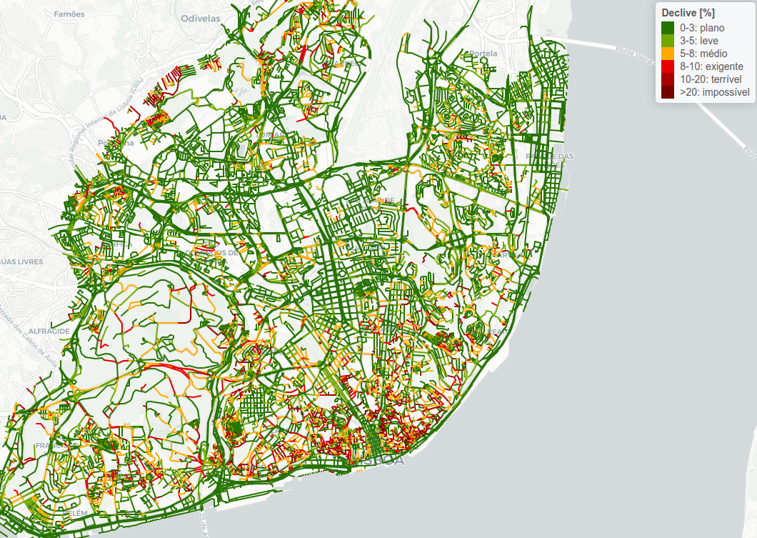
175 | ---
176 |
177 | background-image: url(https://raw.githubusercontent.com/saferactive/saferactive/master/figures/la-multipliers.gif)
178 |
179 | --
180 |
181 | ## Estimating change in exposure
182 |
183 | ### Tackling denominator neglect
184 |
185 | ![]()
186 |
187 | ---
188 |
189 | ## Estimating safety levels in KSI/bkm at high resolution
190 |
191 | 
192 |
193 | ---
194 |
195 | ## Estimating health benefits of cycling uptake with the PCT
196 |
197 | - The PCT uses a modified version of the HEAT methodology to calculate health benefits of scenarios of change
198 | - Based on the DfT's TAG methodology
199 | - The scenarios are **what if** scenarios not forecasts
200 | - See the PCT manual for further information: [pct.bike/manual.html](https://npct.github.io/pct-shiny/regions_www/www/static/03a_manual/pct-bike-eng-user-manual-c1.pdf)
201 | - See the DfT's [AMAT tool](https://assets.publishing.service.gov.uk/government/uploads/system/uploads/attachment_data/file/888754/amat-user-guidance.pdf) also
202 |
203 | 
204 |
205 | ---
206 |
207 | ## From evidence to network plans
208 |
209 | Plans from Leeds City Council responding to national [guidance](https://www.gov.uk/government/publications/reallocating-road-space-in-response-to-covid-19-statutory-guidance-for-local-authorities) and [funding](https://www.gov.uk/government/news/2-billion-package-to-create-new-era-for-cycling-and-walking) for 'pop-up' cycleways (image credit: [Leeds City Council](https://news.leeds.gov.uk/news/leeds-city-council-announces-emergency-walking-and-cycling-plans-in-response-to-covid-19)):
210 |
211 |
212 | 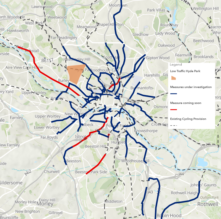
213 |
214 | ---
215 |
216 | background-image: url(https://raw.githubusercontent.com/cyipt/popupCycleways/master/figures/results-top-leeds.png)
217 |
218 | ## The Rapid tool - see [cyipt.bike/rapid](https://www.cyipt.bike/rapid/)
219 |
220 | ---
221 |
222 | # References
223 |
224 | ```{r, 'refs', results="asis", echo=FALSE}
225 | PrintBibliography(my_bib)
226 | # RefManageR::WriteBib(my_bib, "refs-geostat.bib")
227 | ```
228 |
229 |
230 |
231 |
232 |
233 |
234 |
235 |
236 |
237 |
238 |
239 |
240 |
241 |
242 |
243 |
244 |
245 |
246 |
247 |
248 |
249 |
250 |
251 |
252 |
253 |
254 |
255 |
--------------------------------------------------------------------------------
/data-raw/test-pct.R:
--------------------------------------------------------------------------------
1 | # Aim: test the pct pkg can reproduce data on www.pct.bike
2 |
3 | # see https://github.com/ITSLeeds/pct/issues/65#issuecomment-674237160
4 |
5 | # Uptake formula from
6 | # https://raw.githubusercontent.com/npct/pct-shiny/a59ebd1619af4400eeb7ffb2a8ecdd8ce4c3753d/regions_www/www/static/03a_manual/pct-bike-eng-user-manual-c1.pdf
7 | #
8 | # logit (pcycle)= -4.018 + (-0.6369 * distance) +
9 | # (1.988 * distancesqrt) + (0.008775* distancesq) +
10 | # (-0.2555* gradient) + (0.02006* distance*gradient) +
11 | # (-0.1234* distancesqrt*gradient)
12 | library(pct)
13 |
14 | l_pct_2020 = get_pct_lines(region = "isle-of-wight")
15 | pcycle_pct_2019 = uptake_pct_govtarget(distance = l_pct_2020$rf_dist_km, gradient = l_pct_2020$rf_avslope_perc)
16 | summary(pcycle_pct_2019)
17 | # Min. 1st Qu. Median Mean 3rd Qu. Max.
18 | # 0.004712 0.007869 0.011871 0.014671 0.020958 0.043210
19 | govtarget_slc_2019 = round(pcycle_pct_2019 * l_pct_2020$all + l_pct_2020$bicycle)
20 |
21 | cor(l_pct_2020$govtarget_slc, govtarget_slc_2019) # 0.9953986
22 | round(1 - mean(govtarget_slc_2019) / mean(l_pct_2020$govtarget_slc), digits = 5) * 100
23 | # [1] 4.774 # values in pct package 2019 are 5% lower
24 |
25 | # previous (2019) values:
26 | alpha = -3.959
27 | d1 = -0.5963
28 | d2 = 1.866
29 | d3 = 0.008050
30 | h1 = -0.2710
31 | i1 = 0.009394
32 | i2 = -0.05135
33 |
34 | # New (2020) values:
35 | alpha = -4.018
36 | d1 = -0.6369
37 | d2 = 1.988
38 | d3 = 0.008775
39 | h1 = -0.2555
40 | i1 = 0.02006
41 | i2 = -0.1234
42 |
43 | # try to reproduce 2020 values:
44 | pcycle_pct_2020 = uptake_pct_govtarget(
45 | distance = l_pct_2020$rf_dist_km,
46 | gradient = l_pct_2020$rf_avslope_perc,
47 | alpha = alpha,
48 | d1 = d1,
49 | d2 = d2,
50 | d3 = d3,
51 | h1 = h1,
52 | i1 = i1,
53 | i2 = i2
54 | )
55 |
56 | govtarget_slc_2020 = round(pcycle_pct_2020 * l_pct_2020$all + l_pct_2020$bicycle)
57 | cor(l_pct_2020$govtarget_slc, govtarget_slc_2020) # 0.9953986
58 | round(1 - mean(govtarget_slc_2020) / mean(l_pct_2020$govtarget_slc), digits = 5) * 100
59 | # 11.599
60 |
61 | # from 1st principles
62 | l_pct_2020 = pct::get_pct_lines(region = "isle-of-wight")
63 | l_pct_2020$rf_avslope_perc
64 | l_pct_2020$rf_dist_km
65 | uptake_pct_govtarget_2020 = function(
66 | distance,
67 | gradient,
68 | alpha = -4.018,
69 | d1 = -0.6369,
70 | d2 = 1.988,
71 | d3 = 0.008775,
72 | h1 = -0.2555,
73 | i1 = 0.02006,
74 | i2 = -0.1234
75 | ) {
76 | ned_rf_avslope_perc = gradient - 0.78
77 | distancesqrt = sqrt(distance)
78 | distancesq = distance^2
79 | logit_pcycle = alpha + (d1 * distance) +
80 | (d2 * distancesqrt) + (d3 * distancesq) +
81 | (h1 * ned_rf_avslope_perc) + (i1 * distance*ned_rf_avslope_perc) +
82 | (i2* distancesqrt*ned_rf_avslope_perc)
83 | boot::inv.logit(logit_pcycle)
84 | }
85 |
86 |
87 | pcycle_pct_2020 = uptake_pct_govtarget_2020(
88 | distance = l_pct_2020$rf_dist_km,
89 | gradient = l_pct_2020$rf_avslope_perc
90 | )
91 |
92 |
93 | govtarget_slc_2020 = pcycle_pct_2020 * l_pct_2020$all + l_pct_2020$bicycle
94 | plot(l_pct_2020$govtarget_slc, govtarget_slc_2020)
95 | cor(l_pct_2020$govtarget_slc, govtarget_slc_2020) # 0.9928463
96 | round(1 - mean(govtarget_slc_2020) / mean(l_pct_2020$govtarget_slc), digits = 5) * 100
97 | # New estimate is less than 0.3% out
98 |
99 | # test on national data ---------------------------------------------------
100 |
101 | download.file("https://github.com/npct/pct-outputs-national/raw/master/commute/msoa/l_all.Rds",
102 | "l_all.Rds", mode = "wb")
103 | l_all = readRDS("l_all.Rds")
104 |
105 | pcycle_govtarget_uptake = pct::uptake_pct_govtarget(distance = l_all$rf_dist_km, gradient = l_all$rf_avslope_perc)
106 | uptake_pct = round(pcycle_govtarget_uptake * l_all$all + l_all$bicycle)
107 |
108 | summary(l_all$govtarget_slc)
109 | # Min. 1st Qu. Median Mean 3rd Qu. Max.
110 | # 0.000 0.050 0.200 2.579 1.420 715.130
111 | summary(uptake_pct)
112 | # Min. 1st Qu. Median Mean 3rd Qu. Max.
113 | # 0.000 0.000 0.000 2.275 1.000 700.000
114 | plot(l_all$govtarget_slc, uptake_pct)
115 | cor(l_all$govtarget_slc, uptake_pct)
116 | # 0.9976965
117 | round(1 - mean(uptake_pct) / mean(l_all$govtarget_slc), digits = 5) * 100
118 | # [1] 11.773 # values in pct package are 12% lower
119 |
120 |
121 |
--------------------------------------------------------------------------------
/data-raw/test-setup2.R:
--------------------------------------------------------------------------------
1 | # Aim: test set-up for PCT training course
2 | # A version that provides more explanation and analysis
3 |
4 | # test you can install packages
5 | install.packages("remotes", quiet = TRUE)
6 |
7 | # test you have the right packages installed
8 | pkgs = c("sf", "stplanr", "pct", "tmap", "dplyr")
9 | remotes::install_cran(pkgs, quiet = TRUE)
10 |
11 | # load packages
12 | library(sf)
13 | library(tidyverse)
14 | library(pct)
15 | library(tmap)
16 | tmap_mode("view")
17 |
18 | # test you can read-in csv files:
19 | od_data = read.csv("https://github.com/npct/pct-outputs-regional-notR/raw/master/commute/msoa/avon/od_attributes.csv")
20 |
21 | od_data$pcycle = od_data$bicycle / od_data$all
22 | # plot(od_data$rf_dist_km, od_data$pcycle, cex = od_data$all / mean(od_data$all))
23 | ggplot(data = od_data) +
24 | geom_point(aes(x = rf_dist_km, y = pcycle, size = all), alpha = 0.1) +
25 | geom_smooth(aes(x = rf_dist_km, y = pcycle, size = all)) +
26 | ylim(c(0, 0.5))
27 |
28 | # u1 = "https://github.com/npct/pct-outputs-regional-notR/raw/master/commute/msoa/avon/c.geojson"
29 | # u1b = "https://github.com/npct/pct-outputs-regional-notR/raw/master/commute/msoa/avon/z.geojson"
30 | # centroids = read_sf(u1)
31 | # districts = read_sf(u1b)
32 | centroids = get_pct_centroids(region = "avon", geography = "msoa")
33 | districts = get_pct_zones(region = "avon", geography = "msoa")
34 | plot(districts$geometry)
35 | centroids_geo = st_centroid(districts)
36 | plot(centroids$geometry, add = TRUE)
37 | plot(centroids_geo$geometry, add = TRUE, col = "red")
38 |
39 | # check interactive mapping with tmap
40 | u2 = "https://github.com/npct/pct-outputs-regional-notR/raw/master/commute/msoa/avon/l.geojson"
41 | desire_lines = sf::read_sf(u2)
42 | desire_lines_subset = desire_lines[desire_lines$all > 100, ]
43 | tm_shape(desire_lines_subset) +
44 | tm_lines(col = "bicycle", palette = "viridis", lwd = "all", scale = 9)
45 |
46 | # check route network generation with stplanr
47 | # u3 = "https://github.com/npct/pct-outputs-regional-notR/raw/master/commute/msoa/avon/rf.geojson"
48 | # routes = sf::read_sf(u3)
49 | routes = get_pct_routes_fast(region = "avon", geography = "msoa")
50 | routes_1 = routes %>%
51 | slice(which.max(bicycle))
52 | tm_shape(routes_1) +
53 | tm_lines()
54 | routes_30 = routes %>%
55 | top_n(n = 30, wt = bicycle)
56 |
57 | tm_shape(routes_30) +
58 | tm_lines()
59 |
60 | rnet = overline(routes_30, "bicycle")
61 | b = c(0, 0.5, 1, 2, 3, 8) * 1e3
62 | tm_shape(rnet) +
63 | tm_lines(scale = 2, col = "bicycle", palette = "viridis", breaks = b)
64 |
65 | routes$Potential = pct::uptake_pct_godutch_2020(
66 | distance = routes$rf_dist_km,
67 | gradient = routes$rf_avslope_perc
68 | ) *
69 | routes$all +
70 | routes$bicycle
71 |
72 | rnet_potential = overline(routes, "Potential")
73 | tm_shape(rnet_potential) +
74 | tm_lines(lwd = "Potential", scale = 9, col = "Potential", palette = "viridis", breaks = b)
75 |
76 | summary(routes$rf_dist_km)
77 |
78 | ggplot(routes) +
79 | stat_ecdf(aes(rf_dist_km), geom = "step")
80 |
81 | # Uncomment this line to get the mean cycling potential of route segments in Bristol
82 | # round(mean(rnet_potential$Potential))
83 |
84 | # generate output report
85 | # knitr::spin(hair = "code/reproducible-example.R")
86 |
87 | # # to convert OD data into desire lines with the od package you can uncomment the following lines
88 | # # system.time({
89 | # test_desire_lines1 = stplanr::od2line(od_data, centroids)
90 | # # })
91 | # # system.time({
92 | # test_desire_lines2 = od::od_to_sf(x = od_data, z = centroids)
93 | # # })
94 | # plot(test_desire_lines2)
95 |
96 | # test routing on a single line (optional - uncomment to test this)
97 | # warning you can only get a small number, e.g. 5, routes before this stops working!
98 | # library(osrm)
99 | # single_route = route(l = desire_lines[1, ], route_fun = osrm::osrmRoute, returnclass = "sf")
100 | # mapview::mapview(desire_lines[1, ]) +
101 | # mapview::mapview(single_route)
102 | # see https://cran.r-project.org/package=cyclestreets and other routing services
103 | # for other route options, e.g. https://github.com/ropensci/opentripplanner
104 |
105 | # head(od_data_pct[1:12])
106 | # od_data_raw = get_od(region = "avon")
107 | # nrow(od_data_raw)
108 | # nrow(od_data_pct)
109 | # summary(od_data$all)
110 | # summary(od_data_pct$all)
111 | #
112 | # od_data = od_data_raw %>%
113 | # filter(all > 20)
114 | #
115 | # nrow(od_data)
116 | # head(od_data)
117 |
118 | # ggplot(routes) +
119 | # geom_point(aes(dutch_slc, Potential))
120 | # cor(routes$dutch_slc, routes$Potential)^2
121 |
--------------------------------------------------------------------------------
/data-raw/test-setup3.R:
--------------------------------------------------------------------------------
1 | # Test set-up and R packages for estimating cycling potential
2 |
3 | library(sf)
4 | library(tidyverse)
5 | library(stplanr)
6 | library(pct)
7 | library(tmap)
8 |
9 | od_data = od_data = read.csv("https://github.com/npct/pct-outputs-regional-notR/raw/master/commute/msoa/avon/od_attributes.csv")
10 | nrow(od_data)
11 | head(od_data)
12 | od_data$pcycle = od_data$bicycle / od_data$all
13 | plot(od_data$rf_dist_km, od_data$pcycle)
14 | plot(od_data$rf_dist_km, od_data$pcycle, cex = od_data$all / 500)
15 |
16 | # ggplot2
17 | ggplot(od_data) +
18 | geom_point(aes(rf_dist_km, pcycle, size = all), alpha = 0.1) +
19 | geom_smooth(aes(rf_dist_km, pcycle))
20 |
21 | centroids = get_pct_centroids(region = "avon", geography = "msoa")
22 | plot(centroids)
23 | unique(centroids$lad_name)
24 | centroids_bristol = centroids %>%
25 | filter(lad_name == "Bristol, City of")
26 | plot(centroids)
27 | districts = get_pct_zones("avon", geography = "msoa")
28 | districts_bristol = districts %>%
29 | filter(lad_name == "Bristol, City of")
30 | districts_geo_centroid = sf::st_centroid(districts_bristol)
31 | plot(districts_bristol$geometry)
32 | plot(districts_geo_centroid$geometry, col = "red", add = TRUE)
33 | plot(centroids_bristol$geometry, add = TRUE)
34 |
35 | desire_lines = get_pct_lines(region = "avon", geography = "msoa")
36 | desire_lines_bristol = desire_lines %>%
37 | filter(geo_code1 %in% centroids_bristol$geo_code) %>%
38 | filter(geo_code2 %in% centroids_bristol$geo_code)
39 | plot(desire_lines_bristol)
40 | nrow(desire_lines_bristol)
41 |
42 | routes = get_pct_routes_fast(region = "avon", geography = "msoa")
43 | routes_bristol = routes %>%
44 | filter(geo_code1 %in% centroids_bristol$geo_code) %>%
45 | filter(geo_code2 %in% centroids_bristol$geo_code)
46 | mapview::mapview(routes_bristol)
47 |
48 | rnet = overline(routes_bristol, "bicycle")
49 | mapview::mapview(rnet)
50 |
51 | routes$Potential = pct::uptake_pct_godutch(distance = routes$rf_dist_km, gradient = routes$rf_avslope_perc) *
52 | routes$all
53 | rnet_potential = overline(routes, "Potential")
54 | mean(rnet_potential$Potential)
55 |
--------------------------------------------------------------------------------
/data-raw/test-uptake-2020.Rmd:
--------------------------------------------------------------------------------
1 | ---
2 | title: "Testing the PCT uptake formula"
3 | output: html_document
4 | ---
5 |
6 | ```{r setup, include=FALSE}
7 | knitr::opts_chunk$set(echo = TRUE)
8 | ```
9 |
10 | The desire line with the highest potential on the Isle of Wight looks like this:
11 |
12 |
13 | 
14 |
15 | The data hosted on the PCT website provides the same data with more precision:
16 |
17 | ```{r}
18 | library(dplyr)
19 | l = pct::get_pct_lines("isle-of-wight")
20 | l1 = l %>%
21 | filter(bicycle == max(bicycle)) %>%
22 | select(all, bicycle, rf_dist_km, rf_avslope_perc, govtarget_slc, dutch_slc) %>%
23 | sf::st_drop_geometry()
24 | l1
25 | distance = l1$rf_dist_km
26 | ```
27 |
28 | Based on that information we can calculate cycling uptake using the formulae from the manual as follows, first adjusting the hilliness level:
29 |
30 | ```{r}
31 | gradient = l1$rf_avslope_perc - 0.78
32 | ```
33 |
34 | ## Government Target
35 |
36 | The formula to calculate cycling uptake under the Government Target scenario is as follows:
37 |
38 | Equation 1A:
39 |
40 | logit (pcycle) = -4.018 + (-0.6369 * distance) + (1.988 * distance sqrt ) + (0.008775 *
41 | distance sq ) + (-0.2555 * gradient) + (0.02006 * distance*gradient) + (-0.1234 * distance sqrt *gradient)
42 | pcycle
43 | = exp ([logit (pcycle)]) / (1 + (exp([logit(pcycle)])
44 |
45 | In code this can be written as:
46 |
47 | ```{r}
48 | logit_pcycle = -4.018 +
49 | (-0.6369 * distance) +
50 | (1.988 * sqrt(distance)) +
51 | (0.008775 * distance^2) +
52 | (-0.2555 * gradient) +
53 | (0.02006 * distance*gradient) +
54 | (-0.1234 * sqrt(distance) *gradient)
55 | logit_pcycle
56 | pcycle = exp(logit_pcycle) / (1 + exp(logit_pcycle))
57 | ```
58 |
59 | Based on that, the scenario level of cycling would be:
60 |
61 | ```{r}
62 | pcycle
63 | pcycle * l1$all
64 | pcycle * l1$all + l1$bicycle
65 | ```
66 |
67 | Good news, this is the same as the `govtarget_slc` value in the data served by the PCT for that desire line (33 in both cases):
68 |
69 | ```{r}
70 | l1$govtarget_slc
71 | ```
72 |
73 | ## Go Dutch
74 |
75 | Cycling uptake under Go Dutch is calculated as follows.
76 |
77 | Equation 1B:
78 |
79 | logit(pcycle) = = -4.018 + (-0.6369 * distance) + (1.988 * distance sqrt ) + (0.008775 *
80 | distance sq ) + (-0.2555 * gradient) + (0.02006 * distance*gradient) + (-0.1234 * distance sqrt *gradient) + (2.550 *
81 | dutch) + (-0.08036 * dutch * distance)
82 |
83 | Which can be simplified as:
84 |
85 | ```{r}
86 | logit_pcycle = -4.018 + 2.55 +
87 | ((-0.6369 - 0.08036) * distance) +
88 | (1.988 * sqrt(distance)) +
89 | (0.008775 * distance^2) +
90 | (-0.2555 * gradient) +
91 | (0.02006 * distance*gradient) +
92 | (-0.1234 * sqrt(distance) *gradient)
93 | logit_pcycle
94 | pcycle = exp(logit_pcycle) / (1 + exp(logit_pcycle))
95 | ```
96 |
97 | Based on that, the scenario level of cycling would be:
98 |
99 | ```{r}
100 | pcycle
101 | pcycle * l1$all
102 | ```
103 |
104 | However, the `dutch_slc` value in the data served by the PCT for that desire line is slightly higher:
105 |
106 | ```{r}
107 | l1$dutch_slc
108 | ```
109 |
110 |
111 |
112 |
113 | ## Implementing the uptake model in a function
114 |
115 | To ease reproducibility, the uptake formula can be represented in R functions:
116 |
117 | ```{r, eval=FALSE}
118 | remotes::install_github("itsleeds/pct")
119 | ```
120 |
121 |
122 | ```{r}
123 | library(pct)
124 | uptake_pct_govtarget
125 | uptake_pct_godutch_2020
126 | ```
127 |
128 | We can check these reproduce the previous results as follows:
129 |
130 | ```{r}
131 | pcycle * l1$all
132 | uptake_pct_godutch_2020(distance = l1$rf_dist_km, gradient = l1$rf_avslope_perc) *
133 | l1$all
134 | uptake_pct_govtarget_2020(distance = l1$rf_dist_km, gradient = l1$rf_avslope_perc) *
135 | l1$all + l1$bicycle
136 | ```
137 |
138 | ## Overall quality of fit
139 |
140 | At the level of all OD pairs in the small region of the `isle-of-wight`, the correspondence between the results downloaded from the PCT website and the R implementation is as follows:
141 |
142 | ```{r}
143 | pcycle_package_govtarget = uptake_pct_govtarget(l$rf_dist_km, l$rf_avslope_perc)
144 | pcycle_package_godutch = uptake_pct_godutch_2020(l$rf_dist_km, l$rf_avslope_perc)
145 |
146 | govtarget_slc_package = pcycle_package_govtarget * l$all + l$bicycle
147 | godutch_slc_package = pcycle_package_godutch * l$all
148 |
149 | plot(l$govtarget_slc, govtarget_slc_package)
150 | plot(l$dutch_slc, godutch_slc_package)
151 |
152 | cor(l$govtarget_slc, govtarget_slc_package)^2
153 | cor(l$dutch_slc, godutch_slc_package)^2
154 |
155 | cor(l$govtarget_sic, govtarget_slc_package)^2
156 | cor(l$dutch_slc, godutch_slc_package + l$bicycle)^2
157 |
158 | mean(l$govtarget_slc)
159 | mean(govtarget_slc_package)
160 |
161 | -(1 - mean(govtarget_slc_package) /
162 | mean(l$govtarget_slc)) * 100
163 |
164 | -(1 - mean(godutch_slc_package) /
165 | mean(l$dutch_slc)) * 100
166 |
167 | pcycle_gt_package = govtarget_slc_package / l$all
168 | pcycle_gt_web = l$govtarget_slc / l$all
169 |
170 | pcycle_gd_package = godutch_slc_package / l$all
171 | pcycle_gd_web = l$dutch_slc / l$all
172 |
173 | summary(100 * (pcycle_gt_package - pcycle_gt_web))
174 | summary(100 * (pcycle_gd_package - pcycle_gd_web))
175 | ```
176 |
177 |
178 |
--------------------------------------------------------------------------------
/data-raw/workshop-msg.Rmd:
--------------------------------------------------------------------------------
1 | ---
2 | output: github_document
3 | ---
4 |
5 |
6 | ```{r, include=FALSE}
7 | # knitr::opts_chunk$set(echo = FALSE)
8 | # test you can install packages
9 | # install.packages("remotes", quiet = TRUE)
10 |
11 | # test you have the right packages installed
12 | pkgs = c("sf", "stplanr", "pct", "tmap", "dplyr")
13 | remotes::install_cran(pkgs, quiet = TRUE)
14 |
15 | # test you can read-in csv files:
16 | od_data = read.csv("https://github.com/npct/pct-outputs-regional-notR/raw/master/commute/msoa/avon/od_attributes.csv")
17 | head(od_data)
18 | od_data$pcycle = od_data$bicycle / od_data$all
19 | ```
20 |
21 |
22 | Dear Propensity to Cycle Tool Advanced Workshop Participant,
23 |
24 | I am looking forward to the event this Thursday and wanted to share with you a few links and reminders beforehand.
25 |
26 | The **first** thing to say is that this is an **Advanced Workshop** based on the **statistical programming language R** so you will be expected to run code in R/RStudio.
27 | You will be expected to 'get you hands dirty' and write some code so it's important that you have your computer set-up and ready to before the course starts.
28 | To check that R is working on your computer, please ensure that you can run the entirety of this script in RStudio: https://github.com/ITSLeeds/pct/blob/master/inst/test-setup.R
29 |
30 | If you see this plot appear after running line 14 (shown below - see this in context in the link above), congratulations on getting a basic R set-up working.
31 |
32 | ```{r, echo=TRUE}
33 | plot(od_data$rf_dist_km, od_data$pcycle, cex = od_data$all / mean(od_data$all))
34 | ```
35 |
36 |
37 | ```{r, include=FALSE, fig.show='hide'}
38 | # test the sf package: read-in and download zones and centroids
39 | library(sf)
40 | u1 = "https://github.com/npct/pct-outputs-regional-notR/raw/master/commute/msoa/avon/c.geojson"
41 | u1b = "https://github.com/npct/pct-outputs-regional-notR/raw/master/commute/msoa/avon/z.geojson"
42 | centroids = read_sf(u1)
43 | districts = read_sf(u1b)
44 | plot(districts$geometry)
45 | centroids_geo = st_centroid(districts)
46 | plot(centroids$geometry, add = TRUE)
47 | plot(centroids_geo$geometry, add = TRUE, col = "red")
48 |
49 | # check interactive mapping with tmap
50 | library(tmap)
51 | tmap_mode("view")
52 | u2 = "https://github.com/npct/pct-outputs-regional-notR/raw/master/commute/msoa/avon/l.geojson"
53 | desire_lines = sf::read_sf(u2)
54 | desire_lines_subset = desire_lines[desire_lines$all > 100, ]
55 | tm_shape(desire_lines_subset) +
56 | tm_lines(col = "bicycle", palette = "viridis", lwd = "all", scale = 9)
57 |
58 | # check route network generation with stplanr
59 | library(stplanr)
60 | u3 = "https://github.com/npct/pct-outputs-regional-notR/raw/master/commute/msoa/avon/rf.geojson"
61 | routes = sf::read_sf(u3)
62 | library(dplyr)
63 | routes_1 = routes %>%
64 | slice(which.max(bicycle))
65 | tm_shape(routes_1) +
66 | tm_lines()
67 | rnet = overline(routes, "bicycle")
68 | b = c(0, 0.5, 1, 2, 3, 8) * 1e3
69 | tm_shape(rnet) +
70 | tm_lines(scale = 2, col = "bicycle", palette = "viridis", breaks = b)
71 |
72 | # check analysis with dplyr and estimation of cycling uptake with pct function
73 | library(pct)
74 |
75 | routes$Potential = pct::uptake_pct_godutch(
76 | distance = routes$rf_dist_km,
77 | gradient = routes$rf_avslope_perc
78 | ) *
79 | routes$all
80 | rnet_potential = overline(routes, "Potential")
81 | ```
82 |
83 | After running the lines from 15 onwards you should see a number of plots and other outputs.
84 | The following line of code should, after running all the code in the link above, tell you the average number of cyclists on route network segments in Avon under the PCT's Go Dutch scenario:
85 |
86 | ```r
87 | round(mean(rnet_potential$Potential))
88 | ```
89 |
90 | What number did you get? We will test you during the course so make sure you try to reproduce the result.
91 | A more visual check that your computer is set-up to do transport data science with R for modelling cycling uptake is plotting the result.
92 | If you got the plot shown below after running the following [code](https://github.com/ITSLeeds/pct/blob/8fb7b876a3b372c728c8e09f1a2a2004272b37d0/inst/test-setup.R#L59-L60) (you will need to have run all previous lines), congratulations, you're ready to go!
93 |
94 | ```{r}
95 | tm_shape(rnet_potential) +
96 | tm_lines(lwd = "Potential", scale = 9, col = "Potential", palette = "viridis", breaks = b)
97 | ```
98 |
99 | If you have any issues reproducing the code, please double check your R install and make sure you have installed the necessary.
100 |
101 | You will need to have a recent version of R and RStudio installed.
102 | Double check you have at least R 4.0.0 and RStudio 1.2 installed.
103 | If not, [**ensure that you have the latest versions installed**](https://rstudio-education.github.io/hopr/starting.html).
104 |
105 | If you have any issues, please open an issue here: https://github.com/ITSLeeds/pct/issues
106 | (As a last resort you can email at r.lovelace@leeds.ac.uk although I may not be able to respond before the event).
107 |
108 | The **second** thing to say is that having a GitHub account will help you ask questions and share reproducible examples, so please sign-up if you have not yet registered: https://github.com
109 |
110 | After you have signed-up, please check it works by saying hi on this issue (we will also use this link to answer code related questions during the course): https://github.com/ITSLeeds/pct/issues/74
111 |
112 | The **third** thing is about routing. If you want to do routing on the network, please sign-up at https://www.cyclestreets.net/api/apply/. You should save the resulting key on your system by running the following commands:
113 |
114 | ```{r, eval=FALSE}
115 | # uncomment these lines to install cyclestreets
116 | # install.packages("usethis")
117 | # install.packages("cyclestreets")
118 | usethis::edit_r_environ()
119 | ```
120 |
121 | Then add the following line to the file that pops up:
122 |
123 | ```
124 | CYCLESTREETS=ca43ed677e5e6fe1
125 | ```
126 |
127 | For more info on testing if this worked, see:
128 |
129 | The **fourth and final** thing to say: please ensure that you have at least taken a read of (and ideally have reproduced some of the code examples in) these links:
130 |
131 | - The original paper on the Propensity to Cycle Tool: https://www.jtlu.org/index.php/jtlu/article/view/862
132 | - The transport chapter ([12](https://geocompr.robinlovelace.net/transport.html)) in the open source book [*Geocomputation with R*](https://geocompr.robinlovelace.net/)
133 | - The vignette that describes the pct R package, which can be found here: https://itsleeds.github.io/pct/articles/pct.html
134 | - Information on how to create reproducible examples (this will be useful when asking for help during the workshop): https://reprex.tidyverse.org/
135 |
136 | Hope this is useful, please prioritise getting R up-and-running and let us know if you have any issues.
137 |
138 | All the best,
139 |
140 | Robin
141 |
142 | P.s. there is one more thing to say: we plan a virtual 'to the pub' session after the event from 5pm to 6pm so make sure you have beer (or whatever refreshment takes your fancy) in stock if you want to join for a post workshop social.
143 |
--------------------------------------------------------------------------------
/data-raw/workshop-msg.md:
--------------------------------------------------------------------------------
1 |
2 | Dear Propensity to Cycle Tool Advanced Workshop Participant,
3 |
4 | I am looking forward to the event this Thursday and wanted to share with
5 | you a few links and reminders beforehand.
6 |
7 | The **first** thing to say is that this is an **Advanced Workshop**
8 | based on the **statistical programming language R** so you will be
9 | expected to run code in R/RStudio. You will be expected to ‘get you
10 | hands dirty’ and write some code so it’s important that you have your
11 | computer set-up and ready to before the course starts. To check that R
12 | is working on your computer, please ensure that you can run the entirety
13 | of this script in RStudio:
14 |
'
7 | output:
8 | xaringan::moon_reader:
9 | # css: ["default", "its.css"]
10 | # chakra: libs/remark-latest.min.js
11 | lib_dir: libs
12 | nature:
13 | highlightStyle: github
14 | highlightLines: true
15 | # bibliography:
16 | # - ../vignettes/ref.bib
17 | # - ../vignettes/ref_training.bib
18 | ---
19 |
20 | ```{r setup, include=FALSE, eval=FALSE}
21 | # get citations
22 | refs = RefManageR::ReadZotero(group = "418217", .params = list(collection = "JFR868KJ", limit = 100))
23 | refs_df = as.data.frame(refs)
24 | # View(refs_df)
25 | # citr::insert_citation(bib_file = "vignettes/refs_training.bib")
26 | RefManageR::WriteBib(refs, "refs.bib")
27 | # citr::tidy_bib_file(rmd_file = "vignettes/pct_training.Rmd", messy_bibliography = "vignettes/refs_training.bib")
28 | options(htmltools.dir.version = FALSE)
29 | knitr::opts_chunk$set(message = FALSE)
30 | library(RefManageR)
31 | BibOptions(check.entries = FALSE,
32 | bib.style = "authoryear",
33 | cite.style = 'alphabetic',
34 | style = "markdown",
35 | first.inits = FALSE,
36 | hyperlink = FALSE,
37 | dashed = FALSE)
38 | my_bib = refs
39 | ```
40 |
41 | ```{r, include=FALSE}
42 | library(RefManageR)
43 | my_bib = RefManageR::ReadBib("~/itsleeds/pct/inst/rmd/refs.bib")
44 | ```
45 |
46 | ```{r, eval=FALSE, echo=FALSE, engine='bash'}
47 | # publish results online
48 | cp -Rv ~/itsleeds/pct/data-raw/slides/pct-slides-i* ~/saferactive/site/static/slides/
49 | # cp -Rv inst/rmd/libs ~/saferactive/site/static/slides/
50 | cd ~/saferactive/site
51 | git add -A
52 | git status
53 | git commit -am 'Update slides'
54 | git push
55 | cd -
56 |
57 | ```
58 |
59 |
60 | background-image: url(https://media.giphy.com/media/YlQQYUIEAZ76o/giphy.gif)
61 | background-size: cover
62 | class: center, middle
63 |
64 | # How the PCT works
65 |
66 | ---
67 |
68 | ## The first prototype of the PCT
69 |
70 | - 1st prototype: Hackathon at ODI Leeds in February 2015
71 |
72 | - We identifying key routes and mapped them
73 |
74 | - For description of aims, see Lovelace et al. (2017)
75 |
76 | ```{r, echo=FALSE}
77 | knitr::include_graphics("https://raw.githubusercontent.com/npct/pct-team/master/figures/early.png")
78 | ```
79 |
80 | ---
81 |
82 |
83 |
84 | - Launched in 2017 with the Cycling and Walking Investment Strategy ([CWIS](https://www.gov.uk/government/publications/cycling-and-walking-investment-strategy))
85 |
86 | 
87 |
88 | Photo: demo of the PCT to Secretary of State for Transport ([March 2017](https://environment.leeds.ac.uk/transport/news/article/187/research-showcased-to-secretary-of-state))
89 |
90 | ---
91 |
92 | ## The important of open access models
93 |
94 | 
95 |
96 | ---
97 |
98 | ## The PCT in 2020
99 |
100 | - Now the go-to tool for strategic cycle network planning in England and Wales, used by most local authorities with cycling plans ([source](https://npct.github.io/pct-shiny/regions_www/www/static/03d_other_reports/2019-use-of-pct-report.pdf)).
101 |
102 | .pull-left[
103 |
104 | ## Geographic levels in the PCT
105 |
106 | - Generate and analyse route networks for transport planning with reference to:
107 | - Zones
108 | - Origin-destination (OD) data
109 | - Geographic desire lines
110 | - Route allocation using different routing services
111 | - Route network generation and analysis
112 | ]
113 |
114 | .pull-right[
115 |
116 | 
117 | See these levels at [www.pct.bike](https://www.pct.bike)
118 |
119 | ]
120 |
121 | ---
122 |
123 | background-image: url(https://user-images.githubusercontent.com/1825120/96583573-d3c1eb00-12d4-11eb-88b8-ca78087b63f7.png)
124 |
125 | # Live demo of the PCT for Bristol
126 |
127 | ## See https://www.pct.bike/
128 |
129 | ---
130 |
131 |
132 | .pull-left[
133 |
134 | # Uses of the PCT
135 |
136 | - Visioning
137 | - Planning strategic cycle networks
138 | - Identifying corridors with high latent demand
139 |
140 | Uses that were not initially planned
141 |
142 | - Pop-up cycleway planning
143 | - LTN planning?
144 |
145 | ]
146 |
147 | --
148 |
149 | .pull-right[
150 |
151 | ## Deploying in new contexts
152 |
153 | - Requires survey based or synthetic OD data, to be processed by software developed at Leeds `r Citep(my_bib, "lovelace_stplanr:_2018", .opts = list(cite.style = "authoryear"))`
154 | - For mor on methods, see the [transport chapter](https://geocompr.robinlovelace.net/transport.html) (available free [online](https://geocompr.robinlovelace.net/)) `r Citep(my_bib, "lovelace_geocomputation_2019", .opts = list(cite.style = "authoryear"))`
155 | - Can also be used for specific contexts (e.g. cycling to school, cycling to public transport) `r Citep(my_bib, "goodman_scenarios_2019", .opts = list(cite.style = "authoryear"))`
156 |
157 | ]
158 |
159 | --
160 |
161 | #### For further info, see the training materials at [itsleeds.github.io](https://itsleeds.github.io/pct/articles/pct_training.html)
162 |
163 |
164 | #### Many use cases on the PCT website: [pct.bike/manual.html](https://www.pct.bike/manual.html)
165 |
166 | - Case studies of over a dozen areas, including Greater Manchester and Herefordshire in the manual
167 |
168 | ---
169 |
170 | ## New possibilities in the PCT approach
171 |
172 | See [web.tecnico.ulisboa.pt](http://web.tecnico.ulisboa.pt/~rosamfelix/gis/declives/DeclivesLisboa.html) for interactive map
173 |
174 | 
175 | ---
176 |
177 | background-image: url(https://raw.githubusercontent.com/saferactive/saferactive/master/figures/la-multipliers.gif)
178 |
179 | --
180 |
181 | ## Estimating change in exposure
182 |
183 | ### Tackling denominator neglect
184 |
185 | ![]()
186 |
187 | ---
188 |
189 | ## Estimating safety levels in KSI/bkm at high resolution
190 |
191 | 
192 |
193 | ---
194 |
195 | ## Estimating health benefits of cycling uptake with the PCT
196 |
197 | - The PCT uses a modified version of the HEAT methodology to calculate health benefits of scenarios of change
198 | - Based on the DfT's TAG methodology
199 | - The scenarios are **what if** scenarios not forecasts
200 | - See the PCT manual for further information: [pct.bike/manual.html](https://npct.github.io/pct-shiny/regions_www/www/static/03a_manual/pct-bike-eng-user-manual-c1.pdf)
201 | - See the DfT's [AMAT tool](https://assets.publishing.service.gov.uk/government/uploads/system/uploads/attachment_data/file/888754/amat-user-guidance.pdf) also
202 |
203 | 
204 |
205 | ---
206 |
207 | ## From evidence to network plans
208 |
209 | Plans from Leeds City Council responding to national [guidance](https://www.gov.uk/government/publications/reallocating-road-space-in-response-to-covid-19-statutory-guidance-for-local-authorities) and [funding](https://www.gov.uk/government/news/2-billion-package-to-create-new-era-for-cycling-and-walking) for 'pop-up' cycleways (image credit: [Leeds City Council](https://news.leeds.gov.uk/news/leeds-city-council-announces-emergency-walking-and-cycling-plans-in-response-to-covid-19)):
210 |
211 |
212 | 
213 |
214 | ---
215 |
216 | background-image: url(https://raw.githubusercontent.com/cyipt/popupCycleways/master/figures/results-top-leeds.png)
217 |
218 | ## The Rapid tool - see [cyipt.bike/rapid](https://www.cyipt.bike/rapid/)
219 |
220 | ---
221 |
222 | # References
223 |
224 | ```{r, 'refs', results="asis", echo=FALSE}
225 | PrintBibliography(my_bib)
226 | # RefManageR::WriteBib(my_bib, "refs-geostat.bib")
227 | ```
228 |
229 |
230 |
231 |
232 |
233 |
234 |
235 |
236 |
237 |
238 |
239 |
240 |
241 |
242 |
243 |
244 |
245 |
246 |
247 |
248 |
249 |
250 |
251 |
252 |
253 |
254 |
255 |
--------------------------------------------------------------------------------
/data-raw/test-pct.R:
--------------------------------------------------------------------------------
1 | # Aim: test the pct pkg can reproduce data on www.pct.bike
2 |
3 | # see https://github.com/ITSLeeds/pct/issues/65#issuecomment-674237160
4 |
5 | # Uptake formula from
6 | # https://raw.githubusercontent.com/npct/pct-shiny/a59ebd1619af4400eeb7ffb2a8ecdd8ce4c3753d/regions_www/www/static/03a_manual/pct-bike-eng-user-manual-c1.pdf
7 | #
8 | # logit (pcycle)= -4.018 + (-0.6369 * distance) +
9 | # (1.988 * distancesqrt) + (0.008775* distancesq) +
10 | # (-0.2555* gradient) + (0.02006* distance*gradient) +
11 | # (-0.1234* distancesqrt*gradient)
12 | library(pct)
13 |
14 | l_pct_2020 = get_pct_lines(region = "isle-of-wight")
15 | pcycle_pct_2019 = uptake_pct_govtarget(distance = l_pct_2020$rf_dist_km, gradient = l_pct_2020$rf_avslope_perc)
16 | summary(pcycle_pct_2019)
17 | # Min. 1st Qu. Median Mean 3rd Qu. Max.
18 | # 0.004712 0.007869 0.011871 0.014671 0.020958 0.043210
19 | govtarget_slc_2019 = round(pcycle_pct_2019 * l_pct_2020$all + l_pct_2020$bicycle)
20 |
21 | cor(l_pct_2020$govtarget_slc, govtarget_slc_2019) # 0.9953986
22 | round(1 - mean(govtarget_slc_2019) / mean(l_pct_2020$govtarget_slc), digits = 5) * 100
23 | # [1] 4.774 # values in pct package 2019 are 5% lower
24 |
25 | # previous (2019) values:
26 | alpha = -3.959
27 | d1 = -0.5963
28 | d2 = 1.866
29 | d3 = 0.008050
30 | h1 = -0.2710
31 | i1 = 0.009394
32 | i2 = -0.05135
33 |
34 | # New (2020) values:
35 | alpha = -4.018
36 | d1 = -0.6369
37 | d2 = 1.988
38 | d3 = 0.008775
39 | h1 = -0.2555
40 | i1 = 0.02006
41 | i2 = -0.1234
42 |
43 | # try to reproduce 2020 values:
44 | pcycle_pct_2020 = uptake_pct_govtarget(
45 | distance = l_pct_2020$rf_dist_km,
46 | gradient = l_pct_2020$rf_avslope_perc,
47 | alpha = alpha,
48 | d1 = d1,
49 | d2 = d2,
50 | d3 = d3,
51 | h1 = h1,
52 | i1 = i1,
53 | i2 = i2
54 | )
55 |
56 | govtarget_slc_2020 = round(pcycle_pct_2020 * l_pct_2020$all + l_pct_2020$bicycle)
57 | cor(l_pct_2020$govtarget_slc, govtarget_slc_2020) # 0.9953986
58 | round(1 - mean(govtarget_slc_2020) / mean(l_pct_2020$govtarget_slc), digits = 5) * 100
59 | # 11.599
60 |
61 | # from 1st principles
62 | l_pct_2020 = pct::get_pct_lines(region = "isle-of-wight")
63 | l_pct_2020$rf_avslope_perc
64 | l_pct_2020$rf_dist_km
65 | uptake_pct_govtarget_2020 = function(
66 | distance,
67 | gradient,
68 | alpha = -4.018,
69 | d1 = -0.6369,
70 | d2 = 1.988,
71 | d3 = 0.008775,
72 | h1 = -0.2555,
73 | i1 = 0.02006,
74 | i2 = -0.1234
75 | ) {
76 | ned_rf_avslope_perc = gradient - 0.78
77 | distancesqrt = sqrt(distance)
78 | distancesq = distance^2
79 | logit_pcycle = alpha + (d1 * distance) +
80 | (d2 * distancesqrt) + (d3 * distancesq) +
81 | (h1 * ned_rf_avslope_perc) + (i1 * distance*ned_rf_avslope_perc) +
82 | (i2* distancesqrt*ned_rf_avslope_perc)
83 | boot::inv.logit(logit_pcycle)
84 | }
85 |
86 |
87 | pcycle_pct_2020 = uptake_pct_govtarget_2020(
88 | distance = l_pct_2020$rf_dist_km,
89 | gradient = l_pct_2020$rf_avslope_perc
90 | )
91 |
92 |
93 | govtarget_slc_2020 = pcycle_pct_2020 * l_pct_2020$all + l_pct_2020$bicycle
94 | plot(l_pct_2020$govtarget_slc, govtarget_slc_2020)
95 | cor(l_pct_2020$govtarget_slc, govtarget_slc_2020) # 0.9928463
96 | round(1 - mean(govtarget_slc_2020) / mean(l_pct_2020$govtarget_slc), digits = 5) * 100
97 | # New estimate is less than 0.3% out
98 |
99 | # test on national data ---------------------------------------------------
100 |
101 | download.file("https://github.com/npct/pct-outputs-national/raw/master/commute/msoa/l_all.Rds",
102 | "l_all.Rds", mode = "wb")
103 | l_all = readRDS("l_all.Rds")
104 |
105 | pcycle_govtarget_uptake = pct::uptake_pct_govtarget(distance = l_all$rf_dist_km, gradient = l_all$rf_avslope_perc)
106 | uptake_pct = round(pcycle_govtarget_uptake * l_all$all + l_all$bicycle)
107 |
108 | summary(l_all$govtarget_slc)
109 | # Min. 1st Qu. Median Mean 3rd Qu. Max.
110 | # 0.000 0.050 0.200 2.579 1.420 715.130
111 | summary(uptake_pct)
112 | # Min. 1st Qu. Median Mean 3rd Qu. Max.
113 | # 0.000 0.000 0.000 2.275 1.000 700.000
114 | plot(l_all$govtarget_slc, uptake_pct)
115 | cor(l_all$govtarget_slc, uptake_pct)
116 | # 0.9976965
117 | round(1 - mean(uptake_pct) / mean(l_all$govtarget_slc), digits = 5) * 100
118 | # [1] 11.773 # values in pct package are 12% lower
119 |
120 |
121 |
--------------------------------------------------------------------------------
/data-raw/test-setup2.R:
--------------------------------------------------------------------------------
1 | # Aim: test set-up for PCT training course
2 | # A version that provides more explanation and analysis
3 |
4 | # test you can install packages
5 | install.packages("remotes", quiet = TRUE)
6 |
7 | # test you have the right packages installed
8 | pkgs = c("sf", "stplanr", "pct", "tmap", "dplyr")
9 | remotes::install_cran(pkgs, quiet = TRUE)
10 |
11 | # load packages
12 | library(sf)
13 | library(tidyverse)
14 | library(pct)
15 | library(tmap)
16 | tmap_mode("view")
17 |
18 | # test you can read-in csv files:
19 | od_data = read.csv("https://github.com/npct/pct-outputs-regional-notR/raw/master/commute/msoa/avon/od_attributes.csv")
20 |
21 | od_data$pcycle = od_data$bicycle / od_data$all
22 | # plot(od_data$rf_dist_km, od_data$pcycle, cex = od_data$all / mean(od_data$all))
23 | ggplot(data = od_data) +
24 | geom_point(aes(x = rf_dist_km, y = pcycle, size = all), alpha = 0.1) +
25 | geom_smooth(aes(x = rf_dist_km, y = pcycle, size = all)) +
26 | ylim(c(0, 0.5))
27 |
28 | # u1 = "https://github.com/npct/pct-outputs-regional-notR/raw/master/commute/msoa/avon/c.geojson"
29 | # u1b = "https://github.com/npct/pct-outputs-regional-notR/raw/master/commute/msoa/avon/z.geojson"
30 | # centroids = read_sf(u1)
31 | # districts = read_sf(u1b)
32 | centroids = get_pct_centroids(region = "avon", geography = "msoa")
33 | districts = get_pct_zones(region = "avon", geography = "msoa")
34 | plot(districts$geometry)
35 | centroids_geo = st_centroid(districts)
36 | plot(centroids$geometry, add = TRUE)
37 | plot(centroids_geo$geometry, add = TRUE, col = "red")
38 |
39 | # check interactive mapping with tmap
40 | u2 = "https://github.com/npct/pct-outputs-regional-notR/raw/master/commute/msoa/avon/l.geojson"
41 | desire_lines = sf::read_sf(u2)
42 | desire_lines_subset = desire_lines[desire_lines$all > 100, ]
43 | tm_shape(desire_lines_subset) +
44 | tm_lines(col = "bicycle", palette = "viridis", lwd = "all", scale = 9)
45 |
46 | # check route network generation with stplanr
47 | # u3 = "https://github.com/npct/pct-outputs-regional-notR/raw/master/commute/msoa/avon/rf.geojson"
48 | # routes = sf::read_sf(u3)
49 | routes = get_pct_routes_fast(region = "avon", geography = "msoa")
50 | routes_1 = routes %>%
51 | slice(which.max(bicycle))
52 | tm_shape(routes_1) +
53 | tm_lines()
54 | routes_30 = routes %>%
55 | top_n(n = 30, wt = bicycle)
56 |
57 | tm_shape(routes_30) +
58 | tm_lines()
59 |
60 | rnet = overline(routes_30, "bicycle")
61 | b = c(0, 0.5, 1, 2, 3, 8) * 1e3
62 | tm_shape(rnet) +
63 | tm_lines(scale = 2, col = "bicycle", palette = "viridis", breaks = b)
64 |
65 | routes$Potential = pct::uptake_pct_godutch_2020(
66 | distance = routes$rf_dist_km,
67 | gradient = routes$rf_avslope_perc
68 | ) *
69 | routes$all +
70 | routes$bicycle
71 |
72 | rnet_potential = overline(routes, "Potential")
73 | tm_shape(rnet_potential) +
74 | tm_lines(lwd = "Potential", scale = 9, col = "Potential", palette = "viridis", breaks = b)
75 |
76 | summary(routes$rf_dist_km)
77 |
78 | ggplot(routes) +
79 | stat_ecdf(aes(rf_dist_km), geom = "step")
80 |
81 | # Uncomment this line to get the mean cycling potential of route segments in Bristol
82 | # round(mean(rnet_potential$Potential))
83 |
84 | # generate output report
85 | # knitr::spin(hair = "code/reproducible-example.R")
86 |
87 | # # to convert OD data into desire lines with the od package you can uncomment the following lines
88 | # # system.time({
89 | # test_desire_lines1 = stplanr::od2line(od_data, centroids)
90 | # # })
91 | # # system.time({
92 | # test_desire_lines2 = od::od_to_sf(x = od_data, z = centroids)
93 | # # })
94 | # plot(test_desire_lines2)
95 |
96 | # test routing on a single line (optional - uncomment to test this)
97 | # warning you can only get a small number, e.g. 5, routes before this stops working!
98 | # library(osrm)
99 | # single_route = route(l = desire_lines[1, ], route_fun = osrm::osrmRoute, returnclass = "sf")
100 | # mapview::mapview(desire_lines[1, ]) +
101 | # mapview::mapview(single_route)
102 | # see https://cran.r-project.org/package=cyclestreets and other routing services
103 | # for other route options, e.g. https://github.com/ropensci/opentripplanner
104 |
105 | # head(od_data_pct[1:12])
106 | # od_data_raw = get_od(region = "avon")
107 | # nrow(od_data_raw)
108 | # nrow(od_data_pct)
109 | # summary(od_data$all)
110 | # summary(od_data_pct$all)
111 | #
112 | # od_data = od_data_raw %>%
113 | # filter(all > 20)
114 | #
115 | # nrow(od_data)
116 | # head(od_data)
117 |
118 | # ggplot(routes) +
119 | # geom_point(aes(dutch_slc, Potential))
120 | # cor(routes$dutch_slc, routes$Potential)^2
121 |
--------------------------------------------------------------------------------
/data-raw/test-setup3.R:
--------------------------------------------------------------------------------
1 | # Test set-up and R packages for estimating cycling potential
2 |
3 | library(sf)
4 | library(tidyverse)
5 | library(stplanr)
6 | library(pct)
7 | library(tmap)
8 |
9 | od_data = od_data = read.csv("https://github.com/npct/pct-outputs-regional-notR/raw/master/commute/msoa/avon/od_attributes.csv")
10 | nrow(od_data)
11 | head(od_data)
12 | od_data$pcycle = od_data$bicycle / od_data$all
13 | plot(od_data$rf_dist_km, od_data$pcycle)
14 | plot(od_data$rf_dist_km, od_data$pcycle, cex = od_data$all / 500)
15 |
16 | # ggplot2
17 | ggplot(od_data) +
18 | geom_point(aes(rf_dist_km, pcycle, size = all), alpha = 0.1) +
19 | geom_smooth(aes(rf_dist_km, pcycle))
20 |
21 | centroids = get_pct_centroids(region = "avon", geography = "msoa")
22 | plot(centroids)
23 | unique(centroids$lad_name)
24 | centroids_bristol = centroids %>%
25 | filter(lad_name == "Bristol, City of")
26 | plot(centroids)
27 | districts = get_pct_zones("avon", geography = "msoa")
28 | districts_bristol = districts %>%
29 | filter(lad_name == "Bristol, City of")
30 | districts_geo_centroid = sf::st_centroid(districts_bristol)
31 | plot(districts_bristol$geometry)
32 | plot(districts_geo_centroid$geometry, col = "red", add = TRUE)
33 | plot(centroids_bristol$geometry, add = TRUE)
34 |
35 | desire_lines = get_pct_lines(region = "avon", geography = "msoa")
36 | desire_lines_bristol = desire_lines %>%
37 | filter(geo_code1 %in% centroids_bristol$geo_code) %>%
38 | filter(geo_code2 %in% centroids_bristol$geo_code)
39 | plot(desire_lines_bristol)
40 | nrow(desire_lines_bristol)
41 |
42 | routes = get_pct_routes_fast(region = "avon", geography = "msoa")
43 | routes_bristol = routes %>%
44 | filter(geo_code1 %in% centroids_bristol$geo_code) %>%
45 | filter(geo_code2 %in% centroids_bristol$geo_code)
46 | mapview::mapview(routes_bristol)
47 |
48 | rnet = overline(routes_bristol, "bicycle")
49 | mapview::mapview(rnet)
50 |
51 | routes$Potential = pct::uptake_pct_godutch(distance = routes$rf_dist_km, gradient = routes$rf_avslope_perc) *
52 | routes$all
53 | rnet_potential = overline(routes, "Potential")
54 | mean(rnet_potential$Potential)
55 |
--------------------------------------------------------------------------------
/data-raw/test-uptake-2020.Rmd:
--------------------------------------------------------------------------------
1 | ---
2 | title: "Testing the PCT uptake formula"
3 | output: html_document
4 | ---
5 |
6 | ```{r setup, include=FALSE}
7 | knitr::opts_chunk$set(echo = TRUE)
8 | ```
9 |
10 | The desire line with the highest potential on the Isle of Wight looks like this:
11 |
12 |
13 | 
14 |
15 | The data hosted on the PCT website provides the same data with more precision:
16 |
17 | ```{r}
18 | library(dplyr)
19 | l = pct::get_pct_lines("isle-of-wight")
20 | l1 = l %>%
21 | filter(bicycle == max(bicycle)) %>%
22 | select(all, bicycle, rf_dist_km, rf_avslope_perc, govtarget_slc, dutch_slc) %>%
23 | sf::st_drop_geometry()
24 | l1
25 | distance = l1$rf_dist_km
26 | ```
27 |
28 | Based on that information we can calculate cycling uptake using the formulae from the manual as follows, first adjusting the hilliness level:
29 |
30 | ```{r}
31 | gradient = l1$rf_avslope_perc - 0.78
32 | ```
33 |
34 | ## Government Target
35 |
36 | The formula to calculate cycling uptake under the Government Target scenario is as follows:
37 |
38 | Equation 1A:
39 |
40 | logit (pcycle) = -4.018 + (-0.6369 * distance) + (1.988 * distance sqrt ) + (0.008775 *
41 | distance sq ) + (-0.2555 * gradient) + (0.02006 * distance*gradient) + (-0.1234 * distance sqrt *gradient)
42 | pcycle
43 | = exp ([logit (pcycle)]) / (1 + (exp([logit(pcycle)])
44 |
45 | In code this can be written as:
46 |
47 | ```{r}
48 | logit_pcycle = -4.018 +
49 | (-0.6369 * distance) +
50 | (1.988 * sqrt(distance)) +
51 | (0.008775 * distance^2) +
52 | (-0.2555 * gradient) +
53 | (0.02006 * distance*gradient) +
54 | (-0.1234 * sqrt(distance) *gradient)
55 | logit_pcycle
56 | pcycle = exp(logit_pcycle) / (1 + exp(logit_pcycle))
57 | ```
58 |
59 | Based on that, the scenario level of cycling would be:
60 |
61 | ```{r}
62 | pcycle
63 | pcycle * l1$all
64 | pcycle * l1$all + l1$bicycle
65 | ```
66 |
67 | Good news, this is the same as the `govtarget_slc` value in the data served by the PCT for that desire line (33 in both cases):
68 |
69 | ```{r}
70 | l1$govtarget_slc
71 | ```
72 |
73 | ## Go Dutch
74 |
75 | Cycling uptake under Go Dutch is calculated as follows.
76 |
77 | Equation 1B:
78 |
79 | logit(pcycle) = = -4.018 + (-0.6369 * distance) + (1.988 * distance sqrt ) + (0.008775 *
80 | distance sq ) + (-0.2555 * gradient) + (0.02006 * distance*gradient) + (-0.1234 * distance sqrt *gradient) + (2.550 *
81 | dutch) + (-0.08036 * dutch * distance)
82 |
83 | Which can be simplified as:
84 |
85 | ```{r}
86 | logit_pcycle = -4.018 + 2.55 +
87 | ((-0.6369 - 0.08036) * distance) +
88 | (1.988 * sqrt(distance)) +
89 | (0.008775 * distance^2) +
90 | (-0.2555 * gradient) +
91 | (0.02006 * distance*gradient) +
92 | (-0.1234 * sqrt(distance) *gradient)
93 | logit_pcycle
94 | pcycle = exp(logit_pcycle) / (1 + exp(logit_pcycle))
95 | ```
96 |
97 | Based on that, the scenario level of cycling would be:
98 |
99 | ```{r}
100 | pcycle
101 | pcycle * l1$all
102 | ```
103 |
104 | However, the `dutch_slc` value in the data served by the PCT for that desire line is slightly higher:
105 |
106 | ```{r}
107 | l1$dutch_slc
108 | ```
109 |
110 |
111 |
112 |
113 | ## Implementing the uptake model in a function
114 |
115 | To ease reproducibility, the uptake formula can be represented in R functions:
116 |
117 | ```{r, eval=FALSE}
118 | remotes::install_github("itsleeds/pct")
119 | ```
120 |
121 |
122 | ```{r}
123 | library(pct)
124 | uptake_pct_govtarget
125 | uptake_pct_godutch_2020
126 | ```
127 |
128 | We can check these reproduce the previous results as follows:
129 |
130 | ```{r}
131 | pcycle * l1$all
132 | uptake_pct_godutch_2020(distance = l1$rf_dist_km, gradient = l1$rf_avslope_perc) *
133 | l1$all
134 | uptake_pct_govtarget_2020(distance = l1$rf_dist_km, gradient = l1$rf_avslope_perc) *
135 | l1$all + l1$bicycle
136 | ```
137 |
138 | ## Overall quality of fit
139 |
140 | At the level of all OD pairs in the small region of the `isle-of-wight`, the correspondence between the results downloaded from the PCT website and the R implementation is as follows:
141 |
142 | ```{r}
143 | pcycle_package_govtarget = uptake_pct_govtarget(l$rf_dist_km, l$rf_avslope_perc)
144 | pcycle_package_godutch = uptake_pct_godutch_2020(l$rf_dist_km, l$rf_avslope_perc)
145 |
146 | govtarget_slc_package = pcycle_package_govtarget * l$all + l$bicycle
147 | godutch_slc_package = pcycle_package_godutch * l$all
148 |
149 | plot(l$govtarget_slc, govtarget_slc_package)
150 | plot(l$dutch_slc, godutch_slc_package)
151 |
152 | cor(l$govtarget_slc, govtarget_slc_package)^2
153 | cor(l$dutch_slc, godutch_slc_package)^2
154 |
155 | cor(l$govtarget_sic, govtarget_slc_package)^2
156 | cor(l$dutch_slc, godutch_slc_package + l$bicycle)^2
157 |
158 | mean(l$govtarget_slc)
159 | mean(govtarget_slc_package)
160 |
161 | -(1 - mean(govtarget_slc_package) /
162 | mean(l$govtarget_slc)) * 100
163 |
164 | -(1 - mean(godutch_slc_package) /
165 | mean(l$dutch_slc)) * 100
166 |
167 | pcycle_gt_package = govtarget_slc_package / l$all
168 | pcycle_gt_web = l$govtarget_slc / l$all
169 |
170 | pcycle_gd_package = godutch_slc_package / l$all
171 | pcycle_gd_web = l$dutch_slc / l$all
172 |
173 | summary(100 * (pcycle_gt_package - pcycle_gt_web))
174 | summary(100 * (pcycle_gd_package - pcycle_gd_web))
175 | ```
176 |
177 |
178 |
--------------------------------------------------------------------------------
/data-raw/workshop-msg.Rmd:
--------------------------------------------------------------------------------
1 | ---
2 | output: github_document
3 | ---
4 |
5 |
6 | ```{r, include=FALSE}
7 | # knitr::opts_chunk$set(echo = FALSE)
8 | # test you can install packages
9 | # install.packages("remotes", quiet = TRUE)
10 |
11 | # test you have the right packages installed
12 | pkgs = c("sf", "stplanr", "pct", "tmap", "dplyr")
13 | remotes::install_cran(pkgs, quiet = TRUE)
14 |
15 | # test you can read-in csv files:
16 | od_data = read.csv("https://github.com/npct/pct-outputs-regional-notR/raw/master/commute/msoa/avon/od_attributes.csv")
17 | head(od_data)
18 | od_data$pcycle = od_data$bicycle / od_data$all
19 | ```
20 |
21 |
22 | Dear Propensity to Cycle Tool Advanced Workshop Participant,
23 |
24 | I am looking forward to the event this Thursday and wanted to share with you a few links and reminders beforehand.
25 |
26 | The **first** thing to say is that this is an **Advanced Workshop** based on the **statistical programming language R** so you will be expected to run code in R/RStudio.
27 | You will be expected to 'get you hands dirty' and write some code so it's important that you have your computer set-up and ready to before the course starts.
28 | To check that R is working on your computer, please ensure that you can run the entirety of this script in RStudio: https://github.com/ITSLeeds/pct/blob/master/inst/test-setup.R
29 |
30 | If you see this plot appear after running line 14 (shown below - see this in context in the link above), congratulations on getting a basic R set-up working.
31 |
32 | ```{r, echo=TRUE}
33 | plot(od_data$rf_dist_km, od_data$pcycle, cex = od_data$all / mean(od_data$all))
34 | ```
35 |
36 |
37 | ```{r, include=FALSE, fig.show='hide'}
38 | # test the sf package: read-in and download zones and centroids
39 | library(sf)
40 | u1 = "https://github.com/npct/pct-outputs-regional-notR/raw/master/commute/msoa/avon/c.geojson"
41 | u1b = "https://github.com/npct/pct-outputs-regional-notR/raw/master/commute/msoa/avon/z.geojson"
42 | centroids = read_sf(u1)
43 | districts = read_sf(u1b)
44 | plot(districts$geometry)
45 | centroids_geo = st_centroid(districts)
46 | plot(centroids$geometry, add = TRUE)
47 | plot(centroids_geo$geometry, add = TRUE, col = "red")
48 |
49 | # check interactive mapping with tmap
50 | library(tmap)
51 | tmap_mode("view")
52 | u2 = "https://github.com/npct/pct-outputs-regional-notR/raw/master/commute/msoa/avon/l.geojson"
53 | desire_lines = sf::read_sf(u2)
54 | desire_lines_subset = desire_lines[desire_lines$all > 100, ]
55 | tm_shape(desire_lines_subset) +
56 | tm_lines(col = "bicycle", palette = "viridis", lwd = "all", scale = 9)
57 |
58 | # check route network generation with stplanr
59 | library(stplanr)
60 | u3 = "https://github.com/npct/pct-outputs-regional-notR/raw/master/commute/msoa/avon/rf.geojson"
61 | routes = sf::read_sf(u3)
62 | library(dplyr)
63 | routes_1 = routes %>%
64 | slice(which.max(bicycle))
65 | tm_shape(routes_1) +
66 | tm_lines()
67 | rnet = overline(routes, "bicycle")
68 | b = c(0, 0.5, 1, 2, 3, 8) * 1e3
69 | tm_shape(rnet) +
70 | tm_lines(scale = 2, col = "bicycle", palette = "viridis", breaks = b)
71 |
72 | # check analysis with dplyr and estimation of cycling uptake with pct function
73 | library(pct)
74 |
75 | routes$Potential = pct::uptake_pct_godutch(
76 | distance = routes$rf_dist_km,
77 | gradient = routes$rf_avslope_perc
78 | ) *
79 | routes$all
80 | rnet_potential = overline(routes, "Potential")
81 | ```
82 |
83 | After running the lines from 15 onwards you should see a number of plots and other outputs.
84 | The following line of code should, after running all the code in the link above, tell you the average number of cyclists on route network segments in Avon under the PCT's Go Dutch scenario:
85 |
86 | ```r
87 | round(mean(rnet_potential$Potential))
88 | ```
89 |
90 | What number did you get? We will test you during the course so make sure you try to reproduce the result.
91 | A more visual check that your computer is set-up to do transport data science with R for modelling cycling uptake is plotting the result.
92 | If you got the plot shown below after running the following [code](https://github.com/ITSLeeds/pct/blob/8fb7b876a3b372c728c8e09f1a2a2004272b37d0/inst/test-setup.R#L59-L60) (you will need to have run all previous lines), congratulations, you're ready to go!
93 |
94 | ```{r}
95 | tm_shape(rnet_potential) +
96 | tm_lines(lwd = "Potential", scale = 9, col = "Potential", palette = "viridis", breaks = b)
97 | ```
98 |
99 | If you have any issues reproducing the code, please double check your R install and make sure you have installed the necessary.
100 |
101 | You will need to have a recent version of R and RStudio installed.
102 | Double check you have at least R 4.0.0 and RStudio 1.2 installed.
103 | If not, [**ensure that you have the latest versions installed**](https://rstudio-education.github.io/hopr/starting.html).
104 |
105 | If you have any issues, please open an issue here: https://github.com/ITSLeeds/pct/issues
106 | (As a last resort you can email at r.lovelace@leeds.ac.uk although I may not be able to respond before the event).
107 |
108 | The **second** thing to say is that having a GitHub account will help you ask questions and share reproducible examples, so please sign-up if you have not yet registered: https://github.com
109 |
110 | After you have signed-up, please check it works by saying hi on this issue (we will also use this link to answer code related questions during the course): https://github.com/ITSLeeds/pct/issues/74
111 |
112 | The **third** thing is about routing. If you want to do routing on the network, please sign-up at https://www.cyclestreets.net/api/apply/. You should save the resulting key on your system by running the following commands:
113 |
114 | ```{r, eval=FALSE}
115 | # uncomment these lines to install cyclestreets
116 | # install.packages("usethis")
117 | # install.packages("cyclestreets")
118 | usethis::edit_r_environ()
119 | ```
120 |
121 | Then add the following line to the file that pops up:
122 |
123 | ```
124 | CYCLESTREETS=ca43ed677e5e6fe1
125 | ```
126 |
127 | For more info on testing if this worked, see:
128 |
129 | The **fourth and final** thing to say: please ensure that you have at least taken a read of (and ideally have reproduced some of the code examples in) these links:
130 |
131 | - The original paper on the Propensity to Cycle Tool: https://www.jtlu.org/index.php/jtlu/article/view/862
132 | - The transport chapter ([12](https://geocompr.robinlovelace.net/transport.html)) in the open source book [*Geocomputation with R*](https://geocompr.robinlovelace.net/)
133 | - The vignette that describes the pct R package, which can be found here: https://itsleeds.github.io/pct/articles/pct.html
134 | - Information on how to create reproducible examples (this will be useful when asking for help during the workshop): https://reprex.tidyverse.org/
135 |
136 | Hope this is useful, please prioritise getting R up-and-running and let us know if you have any issues.
137 |
138 | All the best,
139 |
140 | Robin
141 |
142 | P.s. there is one more thing to say: we plan a virtual 'to the pub' session after the event from 5pm to 6pm so make sure you have beer (or whatever refreshment takes your fancy) in stock if you want to join for a post workshop social.
143 |
--------------------------------------------------------------------------------
/data-raw/workshop-msg.md:
--------------------------------------------------------------------------------
1 |
2 | Dear Propensity to Cycle Tool Advanced Workshop Participant,
3 |
4 | I am looking forward to the event this Thursday and wanted to share with
5 | you a few links and reminders beforehand.
6 |
7 | The **first** thing to say is that this is an **Advanced Workshop**
8 | based on the **statistical programming language R** so you will be
9 | expected to run code in R/RStudio. You will be expected to ‘get you
10 | hands dirty’ and write some code so it’s important that you have your
11 | computer set-up and ready to before the course starts. To check that R
12 | is working on your computer, please ensure that you can run the entirety
13 | of this script in RStudio:
14 | }}\preformatted{logit (pcycle) = -3.959 + # alpha
127 | (-0.5963 * distance) + # d1
128 | (1.866 * distancesqrt) + # d2
129 | (0.008050 * distancesq) + # d3
130 | (-0.2710 * gradient) + # h1
131 | (0.009394 * distance * gradient) + # i1
132 | (-0.05135 * distancesqrt *gradient) # i2
133 |
134 | pcycle = exp ([logit (pcycle)]) / (1 + (exp([logit(pcycle)])
135 | }\if{html}{\out{
}}
136 |
137 | \code{uptake_pct_govtarget_2020()} and
138 | \code{uptake_pct_godutch_2020()}
139 | approximate the uptake models used in the updated 2020 release of
140 | the PCT results.
141 |
142 | If the \code{distance} parameter is greater than 100, it is assumed that it is in m.
143 | If for some reason you want to model cycling uptake associated with trips with
144 | distances of less than 100 m, convert the distances to km first.
145 | }
146 | \examples{
147 | distance = 15
148 | gradient = 2
149 | logit_pcycle = -3.959 + # alpha
150 | (-0.5963 * distance) + # d1
151 | (1.866 * sqrt(distance)) + # d2
152 | (0.008050 * distance^2) + # d3
153 | (-0.2710 * gradient) + # h1
154 | (0.009394 * distance * gradient) + # i1
155 | (-0.05135 * sqrt(distance) * gradient) # i2
156 | boot::inv.logit(logit_pcycle)
157 | uptake_pct_govtarget(15, 2)
158 | l = routes_fast_leeds
159 | pcycle_scenario = uptake_pct_govtarget(l$length, l$av_incline)
160 | pcycle_scenario_2020 = uptake_pct_govtarget_2020(l$length, l$av_incline)
161 | plot(l$length, pcycle_scenario, ylim = c(0, 0.2))
162 | points(l$length, pcycle_scenario_2020, col = "blue")
163 |
164 | # compare with published PCT data:
165 | \dontrun{
166 | l_pct_2020 = get_pct_lines(region = "isle-of-wight")
167 | # test for another region:
168 | # l_pct_2020 = get_pct_lines(region = "west-yorkshire")
169 | l_pct_2020$rf_avslope_perc[1:5]
170 | l_pct_2020$rf_dist_km[1:5]
171 | govtarget_slc = uptake_pct_govtarget(
172 | distance = l_pct_2020$rf_dist_km,
173 | gradient = l_pct_2020$rf_avslope_perc
174 | ) * l_pct_2020$all + l_pct_2020$bicycle
175 | govtarget_slc_2020 = uptake_pct_govtarget_2020(
176 | distance = l_pct_2020$rf_dist_km,
177 | gradient = l_pct_2020$rf_avslope_perc
178 | ) * l_pct_2020$all + l_pct_2020$bicycle
179 | mean(l_pct_2020$govtarget_slc)
180 | mean(govtarget_slc)
181 | mean(govtarget_slc_2020)
182 | godutch_slc = uptake_pct_godutch(
183 | distance = l_pct_2020$rf_dist_km,
184 | gradient = l_pct_2020$rf_avslope_perc
185 | ) * l_pct_2020$all + l_pct_2020$bicycle
186 | godutch_slc_2020 = uptake_pct_godutch_2020(
187 | distance = l_pct_2020$rf_dist_km,
188 | gradient = l_pct_2020$rf_avslope_perc
189 | ) * l_pct_2020$all + l_pct_2020$bicycle
190 | mean(l_pct_2020$dutch_slc)
191 | mean(godutch_slc)
192 | mean(godutch_slc_2020)
193 | }
194 | # Take an origin destination (OD) pair between an LSOA centroid and a
195 | # secondary school. In this OD pair, 30 secondary school children travel, of
196 | # whom 3 currently cycle. The fastest route distance is 3.51 km and the
197 | # gradient is 1.11\%. The
198 | # gradient as centred on Dutch hilliness levels is 1.11 – 0.63 = 0.48\%.
199 | # The observed number of cyclists is 2. ... Modelled baseline= 30 * .0558 = 1.8.
200 | uptake_pct_govtarget_school2(3.51, 1.11)
201 | # pcycle = exp ([logit (pcycle)])/(1 + (exp([logit(pcycle)]))).
202 | # pcycle = exp(1.953)/(1 + exp(1.953)) = .8758, or 87.58\%.
203 | uptake_pct_godutch_school2(3.51, 1.11)
204 | }
205 |
--------------------------------------------------------------------------------
/man/wight_lines_30.Rd:
--------------------------------------------------------------------------------
1 | % Generated by roxygen2: do not edit by hand
2 | % Please edit documentation in R/data.R
3 | \docType{data}
4 | \name{wight_lines_30}
5 | \alias{wight_lines_30}
6 | \alias{wight_lines_pct}
7 | \title{Desire lines from the PCT for the Isle of Wight}
8 | \description{
9 | This data was obtained using code shown in the introductory
10 | \href{https://itsleeds.github.io/pct/articles/pct.html}{pct package vignette}.
11 | }
12 | \examples{
13 | names(wight_lines_30)
14 | plot(wight_lines_30)
15 | }
16 | \keyword{datasets}
17 |
--------------------------------------------------------------------------------
/man/wight_od.Rd:
--------------------------------------------------------------------------------
1 | % Generated by roxygen2: do not edit by hand
2 | % Please edit documentation in R/data.R
3 | \docType{data}
4 | \name{wight_od}
5 | \alias{wight_od}
6 | \title{Official origin-destination data for the Isle of Wight}
7 | \description{
8 | This data was obtained using code shown in the introductory
9 | \href{https://itsleeds.github.io/pct/articles/pct.html}{pct package vignette}.
10 | }
11 | \examples{
12 | names(wight_od)
13 | head(wight_od)
14 | }
15 | \keyword{datasets}
16 |
--------------------------------------------------------------------------------
/man/wight_routes_30.Rd:
--------------------------------------------------------------------------------
1 | % Generated by roxygen2: do not edit by hand
2 | % Please edit documentation in R/data.R
3 | \docType{data}
4 | \name{wight_routes_30}
5 | \alias{wight_routes_30}
6 | \alias{wight_rnet}
7 | \alias{wight_routes_30_cs}
8 | \title{Cycle route data for the Isle of Wight}
9 | \description{
10 | This data was obtained using code shown in the introductory
11 | \href{https://itsleeds.github.io/pct/articles/pct.html}{pct package vignette}.
12 | }
13 | \examples{
14 | library(sf)
15 | names(wight_routes_30)
16 | head(wight_routes_30)
17 | plot(wight_routes_30)
18 | }
19 | \keyword{datasets}
20 |
--------------------------------------------------------------------------------
/man/wight_zones.Rd:
--------------------------------------------------------------------------------
1 | % Generated by roxygen2: do not edit by hand
2 | % Please edit documentation in R/data.R
3 | \docType{data}
4 | \name{wight_zones}
5 | \alias{wight_zones}
6 | \alias{wight_centroids}
7 | \title{Zones and centroid data from the PCT for the Isle of Wight}
8 | \description{
9 | This data was obtained using code shown in the introductory
10 | \href{https://itsleeds.github.io/pct/articles/pct.html}{pct package vignette}.
11 | }
12 | \examples{
13 | library(sf)
14 | names(wight_lines_30)
15 | plot(wight_lines_30)
16 | }
17 | \keyword{datasets}
18 |
--------------------------------------------------------------------------------
/man/zones_leeds.Rd:
--------------------------------------------------------------------------------
1 | % Generated by roxygen2: do not edit by hand
2 | % Please edit documentation in R/data.R
3 | \docType{data}
4 | \name{zones_leeds}
5 | \alias{zones_leeds}
6 | \title{Zone data for Leeds}
7 | \description{
8 | Zones in Leeds
9 | }
10 | \examples{
11 | # see data-raw folder for generation code
12 | zones_leeds
13 | }
14 | \keyword{datasets}
15 |
--------------------------------------------------------------------------------
/pct-leeds-demo.png:
--------------------------------------------------------------------------------
https://raw.githubusercontent.com/itsleeds/pct/8b68960c60c5e05e782f53e3b259c72ef48f49a6/pct-leeds-demo.png
--------------------------------------------------------------------------------
/pct.Rproj:
--------------------------------------------------------------------------------
1 | Version: 1.0
2 |
3 | RestoreWorkspace: Default
4 | SaveWorkspace: Default
5 | AlwaysSaveHistory: Default
6 |
7 | EnableCodeIndexing: Yes
8 | UseSpacesForTab: Yes
9 | NumSpacesForTab: 2
10 | Encoding: UTF-8
11 |
12 | RnwWeave: Sweave
13 | LaTeX: XeLaTeX
14 |
15 | AutoAppendNewline: Yes
16 | StripTrailingWhitespace: Yes
17 |
18 | BuildType: Package
19 | PackageUseDevtools: Yes
20 | PackageInstallArgs: --no-multiarch --with-keep.source
21 |
--------------------------------------------------------------------------------
/vignettes/.gitignore:
--------------------------------------------------------------------------------
1 | *.html
2 | *.R
3 |
--------------------------------------------------------------------------------
/vignettes/cycling-potential-uk.Rmd:
--------------------------------------------------------------------------------
1 | ---
2 | title: "Cycling potential in UK cities"
3 | output: rmarkdown::html_vignette
4 | vignette: >
5 | %\VignetteIndexEntry{Cycling potential in UK cities}
6 | %\VignetteEngine{knitr::rmarkdown}
7 | %\VignetteEncoding{UTF-8}
8 | ---
9 |
10 | ```{r, include = FALSE}
11 | knitr::opts_chunk$set(
12 | collapse = TRUE,
13 | comment = "#>",
14 | eval = FALSE
15 | )
16 | ```
17 |
18 | Note: this vignette is not evaluated to reduce package build times.
19 | See https://rpubs.com/RobinLovelace/749112 for the results with the code running.
20 |
21 | What modal shift to cycling do you think we could achieve in UK cities in an ideal scenario?
22 | Answers to that question are vital to support high level ambition for active transport and wider sustainability policies in settlements worldwide.
23 | In UK cities such as Leeds (where the motivation for this article originated, via Twitter^[
24 | See `https://twitter.com/PaulChatterton9/status/1190925153322098690` for the original tweet.
25 | ]) there is already a wealth of freely available data on cycling potential, based on the Propensity to Cycle Tool ([PCT](https://www.pct.bike/)) project, of which this package is a part.
26 | This article will briefly explain how to get cycling potential data for any city in England and Wales, based on a case study of Leeds.
27 |
28 | # Getting the region of interest
29 |
30 | The first stage in many projects involving geographic data is to define the region of interest.
31 | In our case we will use the boundary of the Leeds local authority as the basis of analysis.
32 | The PCT is based on 'PCT regions' that we can visualise as follows:
33 |
34 |
35 | ```{r setup, message=FALSE, warning=FALSE}
36 | library(pct)
37 | library(sf)
38 | library(dplyr)
39 | library(tmap)
40 | tm_shape(pct_regions) +
41 | tm_polygons() +
42 | tm_text("region_name", size = 0.6)
43 | ```
44 |
45 | We are interested in Leeds in the `west-yorkshire` area.
46 | Using the `pct` package we can get zone data from the PCT as follows (note: this would work by setting `region_of_interest` to any of the regions shown in the map above:
47 |
48 | ```{r}
49 | region_of_interest = "west-yorkshire"
50 | zones_region = get_pct_zones(region = region_of_interest)
51 | # zones_region = get_pct_zones(region = region_of_interest, geography = "lsoa") # for smaller zones
52 | names(zones_region)
53 | plot(zones_region["bicycle"])
54 | ```
55 |
56 | ```{r, eval=FALSE, echo=FALSE}
57 |
58 | # tm_shape(zones_region) +
59 | # tm_fill("bicycle", palette = "RdYlBu") +
60 | # tm_shape(pct_regions) +
61 | # tm_borders() +
62 | # tm_text("region_name")
63 |
64 | # reproducible example of fail
65 |
66 | remotes::install_github("mtennekes/tmap")
67 | library(tmap)
68 | u = "https://github.com/npct/pct-outputs-regional-notR/raw/master/commute/lsoa/isle-of-wight/z.geojson"
69 | z = sf::st_read(u)
70 | plot(z["bicycle"])
71 | qtm(z)
72 | tm_shape(z) +
73 | tm_fill("bicycle", palette = "RdYlBu")
74 | tmap_mode("view")
75 | qtm(z)
76 |
77 | # another region
78 | tmap_mode("plot")
79 | u = "https://github.com/npct/pct-outputs-regional-notR/raw/master/commute/lsoa/west-yorkshire/z.geojson"
80 | z = sf::st_read(u)
81 | plot(z["bicycle"])
82 | qtm(z)
83 | tm_shape(z) +
84 | tm_fill("bicycle", palette = "RdYlBu")
85 | tmap_mode("view")
86 | qtm(z)
87 | mapview::mapview(z)
88 |
89 | devtools::session_info()
90 | ```
91 |
92 |
93 |
94 | This shows the number of people who say they cycled to work in the 2011 Census.
95 | This may have changed slightly as cycling becomes more popular in some places, but is a good proxy for current cycling levels.
96 | But there are two big problems with this: the map is of West Yorkshire not Leeds, and it's showing current cycling rates, not future potential.
97 |
98 | # Getting cycling potential accross local authorities
99 |
100 | We can find out what local authorities there are in the zones as follows:
101 |
102 | ```{r}
103 | unique(zones_region$lad_name)
104 | ```
105 |
106 | We are interested in the zones in Leeds, which we can get as follows:
107 |
108 | ```{r}
109 | zones = zones_region %>%
110 | filter(lad_name == "Leeds")
111 | tm_shape(zones) +
112 | tm_fill("bicycle", palette = "RdYlBu")
113 | ```
114 |
115 | Great, this represents the current level of cycling across the region of interest.
116 | What about cycling potential? Based on the modelling work in the PCT, we have pre-calculated this for a number of scenarios.
117 | Let's take a look at cycling to work under the Government Target (near market), Go Dutch and Ebikes scenarios for cycling to work:
118 |
119 | ```{r}
120 | scenarios_of_interest = c("govnearmkt_slc", "dutch_slc", "ebike_slc")
121 | tm_shape(zones) +
122 | tm_fill(scenarios_of_interest, palette = "RdYlBu", n = 9, title = "N. cycling") +
123 | tm_facets(nrow = 1, free.scales = FALSE) +
124 | tm_layout(panel.labels = scenarios_of_interest)
125 | ```
126 |
127 | That's great, but it doesn't answer the question of mode share.
128 |
129 | # Cycling mode share
130 |
131 | We can calculate this by dividing the number of people cycling to work by the total:
132 |
133 | ```{r}
134 | zones_mode_share = zones %>%
135 | select(scenarios_of_interest) %>%
136 | mutate_at(scenarios_of_interest, .funs = list(~ ./zones$all * 100))
137 | tm_shape(zones_mode_share) +
138 | tm_fill(scenarios_of_interest, palette = "RdYlBu", title = "% cycling") +
139 | tm_facets(nrow = 1, free.scales = FALSE) +
140 | tm_layout(panel.labels = scenarios_of_interest)
141 | ```
142 |
143 | The summary mode shares can be estimated as follows, with results showing the % cycling currently (according to the 2011 census) and under scenarios of change:
144 |
145 | ```{r}
146 | zones_region %>%
147 | st_drop_geometry() %>%
148 | group_by(lad_name) %>%
149 | select(`2011 census` = bicycle, c(scenarios_of_interest, "all")) %>%
150 | summarise_all(.funs = ~ round(sum(.)/sum(all)* 100)) %>%
151 | select(-all, `Local Authority / % Cycling in scenario:` = lad_name) %>%
152 | knitr::kable()
153 | ```
154 |
155 |
156 |
157 |
158 |
159 | # Cycling potential nationwide
160 |
161 | To generalise the analysis outlined above, we can download national data from the PCT project as follows:
162 |
163 | ```{r national-dl}
164 | zones_national = read_sf("https://github.com/npct/pct-outputs-national/raw/master/commute/msoa/z_all.geojson")
165 | ```
166 |
167 | A summary of cycling potential nationwide can then be calculated as follows:
168 |
169 | ```{r}
170 | national_commute_totals = zones_national %>%
171 | st_drop_geometry() %>%
172 | select(all, census_2011 = bicycle, govtarget_slc, dutch_slc) %>%
173 | summarise_all(.funs = ~sum(.))
174 | national_commute_percentages = national_commute_totals / national_commute_totals$all * 100
175 | ```
176 |
177 | ```{r, echo=FALSE}
178 | knitr::kable(bind_rows(national_commute_totals, national_commute_percentages), digits = 1,
179 | caption = "Total counts and percentages of cycle commuters under different scenarios")
180 | ```
181 |
182 | We can calculate the mode share of cycling under these same scenarios for any area (e.g. the boundary of Greater London) or for a list of named local authorities, as follows:
183 |
184 | ```{r}
185 | r = read.csv(stringsAsFactors = FALSE, text = "area
186 | Greater London
187 | Greater Manchester
188 | Birmingham
189 | Leeds
190 | Glasgow
191 | Liverpool
192 | Newcastle
193 | Bristol
194 | Cardiff
195 | Belfast
196 | Southampton
197 | Sheffield
198 | ")
199 | matching_las = pct_regions_lookup$lad16nm[pct_regions_lookup$lad16nm %in% r$area]
200 | matching_regions = c("london", "greater-manchester")
201 | pct_lookup = pct_regions_lookup %>%
202 | rename(lad_name = lad16nm)
203 | zones_national = inner_join(zones_national, pct_lookup)
204 | zones_national = zones_national %>%
205 | mutate(area = case_when(
206 | region_name == "london" ~ "Greater London",
207 | region_name == "greater-manchester" ~ "Greater Manchester",
208 | lad_name %in% matching_las ~ lad_name,
209 | TRUE ~ "Other"
210 | ))
211 | table(zones_national$area)
212 | zones_aggregated = zones_national %>%
213 | sf::st_drop_geometry() %>%
214 | group_by(area) %>%
215 | summarise(
216 | Commuters = sum(all, na.rm = TRUE),
217 | Bicycle_census = sum(bicycle),
218 | Bicycle_govtarget = sum(govtarget_slc),
219 | Bicycle_godutch = sum(dutch_slc)
220 | )
221 |
222 | # plot(zones_aggregated["Commuters"], border = NA)
223 | zones_aggregated %>%
224 | inner_join(r, .) %>%
225 | knitr::kable(digits = 0)
226 | ```
227 |
228 | Next we can calculate the mode splits as follows:
229 |
230 | ```{r}
231 | zones_aggregated_percents = zones_aggregated %>%
232 | mutate_at(vars(-Commuters, -area), funs(./Commuters * 100))
233 | names(zones_aggregated_percents)[3:5] = paste0(names(zones_aggregated_percents)[3:5], "_percent")
234 | zones_aggregated_percents %>%
235 | inner_join(r, .) %>%
236 | knitr::kable(digits = 1)
237 | ```
238 |
239 | # Considerations
240 |
241 | The results above show that there is huge potential for cycling grow across England and Wales.
242 | Around 16% of commuters in Leeds could cycle to work if we 'Go Dutch' (25% if we Go Dutch and see high uptake of electric bikes) for the single mode journey to work data under consideration.
243 | However, there are some wider considerations that are not captured in the numbers (see the [PCT paper](https://www.jtlu.org/index.php/jtlu/article/view/862) for details and other considerations):
244 |
245 | - The PCT commute layer (don't forget the travel to schools layer!) only considers single stage journeys - if we were to include cycling to the station or bus stop potential it would be greater than 16%, perhaps more like 30% if potential cycle/rail and cycle/bus trips are accounted for.
246 | - Work patterns are changing, and with new digital work practices or a shift towards local economies, more people could work from home or at least near to home.
247 | - The scenarios are snapshots of how cycling levels could change based current trip patterns, not predictions of what will happen. There are many other scenarios that could be developed, including intermediate scenarios between Go Dutch and the Government Target, and more ambitious scenarios, e.g. 'Go Utrecht', where cycling has reached around 60% of trips ([source](https://www.bloomberg.com/news/articles/2019-07-05/how-the-dutch-made-utrecht-a-bicycle-first-city)).
248 |
249 | Other considerations that are often mentioned are hills and people who are unable to cycle.
250 | In fact the PCT accounts for hills and, as the example of Bristol shows, hilly cities can see rapid increases in cycling.
251 | Regarding ability to cycle, it is a more inclusive mode than driving, with 8 to 80 year-olds being able to cycle, and many more people being able to afford a bike than a car (which, thanks to the expense of buying, running and insuring the vehicle, is largely the mode of choice of the wealthy).
252 | The PCT does not account for the fact that some trips to work are also 'caregiving' trips, but with electric cargo bikes and [multi-person cycles](https://en.wikipedia.org/wiki/Cycle_rickshaw) cycling-focused cities can, to a greater extent than car-dominated transport systems, deliver for all.
253 |
254 | ## Challenge
255 |
256 | To anyone interested in cycling in your city: try re-running the reproducible code above for your PCT region and local authority.
257 | Let us know on social media and [GitHub](https://github.com/ITSLeeds/pct/issues) how you get on.
258 | Any comments/contributions to this analysis: [welcome.](https://github.com/ITSLeeds/pct/edit/master/vignettes/cycling-potential-uk.Rmd)
259 |
--------------------------------------------------------------------------------
/vignettes/km-cycled.Rmd:
--------------------------------------------------------------------------------
1 | ---
2 | title: "Estimating distance cycled per zone in England and Wales regions"
3 | output: rmarkdown::html_vignette
4 | vignette: >
5 | %\VignetteIndexEntry{Estimating distance cycled per zone in England and Wales regions}
6 | %\VignetteEngine{knitr::rmarkdown}
7 | %\VignetteEncoding{UTF-8}
8 | author:
9 | - "Nathanael Sheehan"
10 | ---
11 |
12 | In the context of society, cycling acts as a vessel to mobilise citizens to navigate through spatial geography in a sustainable fashion. In doing so, cycling obtains numerous socio-spatial benefits both at the micro (individual health benefits from active transport) and macro (lower pollution from vehicles) scale. With the ambition of building a sustainable future, the PCT project promotes cycle uptake through providing open tools for policy-makers, transport planners and academics to plan future cycle infrastructure for the built environment.
13 |
14 | Using data from the 2011 census and models built into the PCT package, this article asks the question of "How many km's per LSOA do commuters cycle through each year?". The results of which provide valuable insight into future sustainable transport planning decisions and highlight the versatility of the PCT package through a reproducible method.
15 |
16 | Set `eval=TRUE` to run this code when knitting:
17 |
18 | ```{r}
19 | knitr::opts_chunk$set(eval = FALSE)
20 | ```
21 |
22 |
23 | ## Prerequisites
24 |
25 | The following packages must be installed and loaded to run the code in this vignette.
26 |
27 | ```{r, message=FALSE, warning=FALSE}
28 | # Load packages
29 | library(pct)
30 | library(tmap)
31 | ```
32 |
33 | ## Estimating distance cycled for a region based on 2011 census data
34 |
35 | The PCT package permits an easy method for fetching road network and commuting origin/destination data for any region in England and Wales. This data will be used as the basis for understanding the current context of cycling for a given region (A definition of regions can be found in this earlier article). For this first example, we will apply the pct method to the region of Oxfordshire. To kick things off, we use the ```get_pct_rnet``` to retrieve road network data for the region. This data is then used to calculate the length of the road network cycled using ```base ``` r functions.
36 |
37 | ```{r, message=FALSE, warning=FALSE}
38 | #Get road network for preselected regin
39 | rnet = pct::get_pct_rnet(region = "oxfordshire")
40 | #Calculate road length
41 | rnet$segment_length = as.numeric(sf::st_length(rnet))
42 | #Calculate daily km's cycled
43 | rnet$m_cycled_per_working_day = rnet$segment_length * rnet$bicycle
44 | ```
45 |
46 | Simples! Now we can use the ```get_pct_zones``` function to get LSOA geographies in order to calculate the number of km's cycled per day through each LSOA.
47 |
48 | ```{r, message=FALSE, warning=FALSE}
49 | # Get road network for preselected regin
50 | zones = pct::get_pct_zones(region = "oxfordshire")
51 | summary(sf::st_is_valid(zones))
52 | zones = sf::st_make_valid(zones)
53 | summary(sf::st_is_valid(zones))
54 | cycled_m_per_zone = aggregate(rnet["m_cycled_per_working_day"], zones, FUN = sum)
55 | ```
56 |
57 | While this is great information, it doesn't provide answer the long term question of how many distance are cycled per year. In order to achieve this, we must multiple the number of trips per day by the number of days in a standard working year (200) and divide by a million. Once again, this is achieved using ```base``` r functionality.
58 |
59 | ```{r, message=FALSE, warning=FALSE}
60 | zones$mkm_cycled_for_commuting_per_year_estimated = cycled_m_per_zone$m_cycled_per_working_day *
61 | 2 * 200 / # estimate of trips days per year, morning and afternoon
62 | 1e9
63 | ```
64 |
65 | With this calculated, we can now answer our question and visualize yearly km's cycled using ```tmap```.
66 |
67 | ```{r, message=FALSE, warning=FALSE, fig.align="center", fig.width = 7, fig.height = 6}
68 | tm_shape(zones) +
69 | tm_fill(
70 | col = "mkm_cycled_for_commuting_per_year_estimated",
71 | style = "quantile",
72 | palette = "plasma",
73 | title = "Yearly distance cycled by commuters per day\n(2011 Census Data)",
74 | legend.size.is.portrait = TRUE
75 | ) +
76 | tm_layout(
77 | title = "OXFORDSHIRE",
78 | title.position = c("left", "top"),
79 | bg.color = "honeydew3",
80 | outer.bg.color = "honeydew",
81 | legend.stack = "horizontal",
82 | legend.outside = TRUE,
83 | legend.outside.position = "left",
84 | frame.lwd = 5
85 | )
86 | ```
87 |
88 | Wow, that's a lot of miles cycled! The plot breaks down the number km's cycled by quartiles and thus paints the picture of where cycling is most prominent. In the context of Oxfordshire, the map depecits the region obtainaing a rather high cycle uptake; with its spatial distribution primarily in the centre of the region.
89 |
90 | ## Comparing Regions
91 |
92 | Now say we wanted to compare the results of Oxfordshire, with its regional neighbor Cambridgeshire. This can be achieved by wrapping the previous method into a function.
93 |
94 | ```{r, message=FALSE, warning=FALSE}
95 | pct_zones_rnet_current = function(region_name) {
96 | # Get road network for preselected regin
97 | rnet = pct::get_pct_rnet(region = region_name)
98 | # Calculate road length
99 | rnet$segment_length = as.numeric(sf::st_length(rnet))
100 | # Calculate daily km cycled
101 | rnet$m_cycled_per_working_day = rnet$segment_length * rnet$bicycle
102 | # Convert to centroids to avoid double counting flows that cross zones
103 | rnet_centroids = sf::st_centroid(rnet)
104 | # Get LSOA spatial data
105 | zones = sf::st_make_valid(pct::get_pct_zones(region = region_name))
106 | # Calculate cyced miles per zone
107 | cycled_m_per_zone = aggregate(rnet_centroids["m_cycled_per_working_day"], zones, FUN = sum)
108 | # Calculate miles cycled per year from commuting
109 | zones$mkm_cycled_for_commuting_per_year_estimated = cycled_m_per_zone$m_cycled_per_working_day *
110 | 2 * 200 / # estimate of trips days per year, morning and afternoon
111 | 1e9
112 | # Plot results
113 | tmap_mode("plot")
114 | tm_shape(zones) +
115 | tm_fill(
116 | col = "mkm_cycled_for_commuting_per_year_estimated",
117 | style = "quantile",
118 | palette = "plasma",
119 | title = "Million km's cycled by commuters per year\n(2011 Census Data)",
120 | legend.size.is.portrait = TRUE
121 | ) +
122 | tm_layout(
123 | title = toupper(region_name),
124 | title.position = c("left", "top"),
125 | bg.color = "honeydew3",
126 | outer.bg.color = "honeydew",
127 | legend.stack = "horizontal",
128 | legend.outside = TRUE,
129 | legend.outside.position = "bottom",
130 | frame.lwd = 5
131 | )
132 |
133 | }
134 | ```
135 |
136 | With our function built, we can now easily compare regional differences.
137 |
138 | ```{r, message=FALSE, warning=FALSE, fig.align="center", fig.width = 7, fig.height = 6}
139 | oxfordshire_results = pct_zones_rnet_current(region_name = "oxfordshire")
140 | cambrideshire_results = pct_zones_rnet_current(region_name = "cambridgeshire")
141 | tmap_arrange(oxfordshire_results, cambrideshire_results, ncol = 2)
142 | ```
143 |
144 | In comparison to Oxfordshire, Cambridgeshire spatial distribution of km's cycled exhibit a high number of cycling not only in the centre of the region. While Oxfordshire obtains a zone with a higher number of km's cycled through it, in general Cambridgeshire displays a higher number in its quartile range. Interesting!
145 |
146 | Now lets say we wanted to compare two cities. Lets take London and Greater Manchester.
147 |
148 | ```{r, message=FALSE, warning=FALSE, fig.align="center", fig.width = 7, fig.height = 6}
149 | london_results = pct_zones_rnet_current(region_name = "london")
150 | gm_results = pct_zones_rnet_current(region_name = "greater-manchester")
151 | #tmap_mode("view")
152 | tmap_arrange(london_results, gm_results, ncol = 2)
153 | ```
154 |
155 | Jheeze! The maps provides insight at a highly granular level. Both Greater Manchester and London have similar quartile ranges and are fairly monocentric, however, LSOA's in London such as ```E01032739``` obtain billions in km's cycled per year; likely due to working population differences. Nonetheless, outer LSOA's in both Greater Manchester and London also feature in the highest quartile, representing that cycle uptake is not dominant solely in the centre of the regions.
156 |
157 | ## Using PCT models to visualize potential cycle uptake
158 |
159 | While the results based on the 2011 census provide interesting and valuable results, a lot has changed since 2011 and other scenarios should be explored. The PCT package features numerous models (e.g. ```govtarget_slc```,```gendereq_slc``` and ```ebike_slc```). In this example, lets examine London and Manchester again, but this time, lets use the PCT E-bike model scenario. The PCT E-Bike model assumes commuters will use e-Bikes for longer or hillier trips (based on data from Dutch and Swiss travel surveys). In order to model this, we will build a function similar to what we used for the census data, but change the daily miles cycled to use the ```ebike_slc``` column.
160 |
161 | ```{r, message=FALSE, warning=FALSE}
162 | pct_zones_rnet_ebikes <- function(region_name) {
163 | # Get road network for pre-selected region
164 | rnet = pct::get_pct_rnet(region = region_name)
165 | # Calculate road length
166 | rnet$segment_length = as.numeric(sf::st_length(rnet))
167 | # Calculate daily miles cycled
168 | rnet$m_cycled_per_working_day = rnet$segment_length * rnet$ebike_slc
169 | # Convert to centroids to avoid double counting flows that cross zones
170 | rnet_centroids = sf::st_centroid(rnet)
171 | # Get LSOA spatial data
172 | zones = sf::st_make_valid(pct::get_pct_zones(region = region_name))
173 | # Calculate cycled miles per zone
174 | cycled_m_per_zone = aggregate(rnet_centroids["m_cycled_per_working_day"], zones, FUN = sum)
175 | # Calculate km cycled per year from commuting
176 | zones$mkm_cycled_for_commuting_per_year_estimated = cycled_m_per_zone$m_cycled_per_working_day *
177 | 2 * 200 / # estimate of trips days per year, morning and afternoon
178 | 1e9
179 | #Plot results
180 | tmap_mode("plot")
181 | tm_shape(zones) +
182 | tm_fill(
183 | col = "mkm_cycled_for_commuting_per_year_estimated",
184 | style = "quantile",
185 | palette = "plasma",
186 | title = "Million km's cycled by commuters per year\n(E-Bike model)",
187 | legend.size.is.portrait = TRUE
188 | ) +
189 | tm_layout(
190 | title = toupper(region_name),
191 | title.position = c("left", "top"),
192 | bg.color = "honeydew3",
193 | outer.bg.color = "honeydew",
194 | legend.stack = "horizontal",
195 | legend.outside = TRUE,
196 | legend.outside.position = "bottom",
197 | frame.lwd = 5
198 | )
199 | }
200 | ```
201 |
202 | With our E-Bikes function built, we can map the results to visualise the effect an E-bike scenario may have on these two cities.
203 |
204 | ```{r, message=FALSE, warning=FALSE, fig.align="center", fig.width = 7, fig.height = 6}
205 | london_results_ebikes = pct_zones_rnet_ebikes(region_name = "london")
206 | gm_results_ebikes = pct_zones_rnet_ebikes(region_name = "greater-manchester")
207 | #tmap_mode("view")
208 | tmap_arrange(london_results_ebikes, gm_results_ebikes, ncol = 2)
209 | ```
210 |
211 | Wow! The maps show how an E-Bike scenario could increase cycle uptake by ~500%. As this model illustrates, an E-Bike scenario would mean more LSOA's would be in the highest quartile of distance cycled. This would mean safer roads, cleaner air and a more sustainable future.
212 |
213 | ## Conclusions and next steps
214 |
215 | As demonstrated, the PCT packages provides easy methods to visualize cycle potential. This article has briefly shown how you can use the PCT package models to understand what future cycle uptake could look like and how to calculate the number of km's cycled per year at a granular level. If this article is of use/interest, why not try for your local region showing the potential based on different models. You can also try the following resources (in R and online):
216 |
217 | * Have a play with the PCT web application
218 | * For more of a deep dive into the methods, see the pct_training vignette
219 | * See the pct-international to see how to apply the methods internationally
220 |
221 | We’re interested to know how you’ve used the methods/data so please get in touch on social media and GitHub letting us know how get on. Any comments/contributions to this analysis: welcome.
222 |
--------------------------------------------------------------------------------
/vignettes/nature.csl:
--------------------------------------------------------------------------------
1 |
2 |
126 |
--------------------------------------------------------------------------------
/vignettes/pct-international.Rmd:
--------------------------------------------------------------------------------
1 | ---
2 | title: "International application of the PCT methods"
3 | author: "Robin Lovelace, Layik Hama"
4 | date: "`r Sys.Date()`"
5 | output: rmarkdown::html_vignette
6 | vignette: >
7 | %\VignetteIndexEntry{International application of the PCT}
8 | %\VignetteEngine{knitr::rmarkdown}
9 | %\VignetteEncoding{UTF-8}
10 | ---
11 |
12 | ```{r setup, include = FALSE}
13 | knitr::opts_chunk$set(
14 | collapse = TRUE,
15 | comment = "#>"
16 | )
17 | ```
18 |
19 | ## Introduction
20 |
21 | The package README shows how the PCT can be used to get and reproduce some of the datasets from the PCT package, based on an example in the city of Leeds.
22 | This vignette shows how the package can be used to create estimates of cycling potential in other cities.
23 |
24 | Set `eval=TRUE` to run this code when knitting:
25 |
26 | ```{r}
27 | knitr::opts_chunk$set(eval = FALSE)
28 | ```
29 |
30 | Let's start by loading the package:
31 |
32 | ```{r libraries, message=FALSE}
33 | # devtools::install_github("ATFutures/geoplumber")
34 | # require("geojsonsf")
35 | library(pct)
36 | ```
37 |
38 | ## Input data
39 |
40 | The input data for this vignetted was created using code in the [pctSantiago](https://github.com/pedalea/pctSantiago) project.
41 | It looks like this, in terms of the flow data:
42 |
43 | ```{r}
44 | head(santiago_od)
45 | ```
46 |
47 | In terms of the zone data, they look like this:
48 |
49 | ```{r}
50 | sf:::print.sf(santiago_zones)
51 | plot(santiago_zones)
52 | ```
53 |
54 | Note that we have cycling estimates for each desire line.
55 | If this data is not known, current cycling levels can be approximated for all desire lines as the city-wide average, e.g. around 5% for Santiago.
56 |
57 | ## Creating desire lines
58 |
59 | The origin-destination data can be converted to geographic desire lines using the `stplanr` function `od2line` as follows:
60 |
61 | ```{r, warning=FALSE}
62 | desire_lines = stplanr::od2line(flow = santiago_od, zones = santiago_zones)
63 | ```
64 |
65 | The resulting lines can then be plotted on top of zone data as follows:
66 |
67 | ```{r, out.width="100%"}
68 | plot(santiago_zones$geometry)
69 | plot(santiago_lines["pcycle"], lwd = santiago_lines$n / 3, add = TRUE)
70 | # gj = geojsonsf::sf_geojson(santiago_lines)
71 | # path = file.path(tempdir(), "dl.geojson")
72 | # write(gj, path)
73 | # html_map = geoplumber::gp_map(path, browse_map = FALSE)
74 | # htmltools::includeHTML(html_map)
75 | ```
76 |
77 | The previous map suggests that the data is reliable: we have created a good approximation of the travel pattern in central Santiago.
78 |
79 | ## Estimating cycling uptake
80 |
81 | To estimate cycling potential, we need estimates of distance and hilliness.
82 | The area under investigation is relatively flat so we can make the simplifying assumption that hilliness is 0% for all lines (normally we would get this information from a routing service):
83 |
84 | ```{r}
85 | desire_lines$hilliness = 0
86 | ```
87 |
88 | And what about the distance?
89 | We can calculated it as follows (note we converted this into a numeric object to prevent issues associated with the `units` package):
90 |
91 | ```{r}
92 | desire_lines$distance = as.numeric(sf::st_length(desire_lines))
93 | ```
94 |
95 | Now we have (very) crude estimates of distance and hilliness, we can estimate the cycling potential as follows:
96 |
97 | ```{r}
98 | desire_lines$godutch_pcycle = uptake_pct_godutch(distance = desire_lines$distance, gradient = 0)
99 | ```
100 |
101 | Let's take a look at the results, compared with the current levels of cycling, and compared with distance:
102 |
103 | ```{r}
104 | cor(x = desire_lines$pcycle, y = desire_lines$godutch_pcycle)
105 | plot(x = desire_lines$pcycle, y = desire_lines$godutch_pcycle)
106 | plot(x = desire_lines$distance, y = desire_lines$godutch_pcycle, ylim = c(0, 1))
107 | ```
108 |
109 | As expected, there is a positive (albeit small) positive correlation between current and potential levels of cycling.
110 | The result shows clearly that distance decay kicks in just after 2km, but still at 8 km there is a 25% mode share, suggesting a major switch to cycling.
111 |
112 | We can put the results on a map as follows:
113 |
114 | ```{r, out.width="50%", fig.show='hold'}
115 | library(leaflet)
116 | leaflet(width = "100%") %>%
117 | addTiles() %>%
118 | addPolylines(data = desire_lines, weight = desire_lines$pcycle * 5)
119 | leaflet(width = "100%") %>%
120 | addTiles() %>%
121 | addPolylines(data = desire_lines, weight = desire_lines$godutch_pcycle * 5)
122 | ```
123 |
124 | The results show that there is substantial potential for increasing the levels of cycling in central Santiago, based on origin-destination data alone.
125 | However, to inform policy, more detailed estimates of cycling potential are needed, with results that go down to the level of individual streets.
126 | This involves routing.
127 |
128 | ## Routing
129 |
130 | There are many ways to do calculate a path on the street network.
131 | The main options are local routing, where the calculation is done based on data stored locally (on your computer) and routing services, where the data is done remotely ('in the cloud').
132 | Let's use a remote routing service to convert the straight lines generated in the previous section into routes that could realistically be taken by people cycling (the next line does not run by default because it requires an API key saved as an environment variable, see the [documentation of `route_cyclestreets()` for details](https://docs.ropensci.org/stplanr/reference/index.html#section-routing) for details).
133 |
134 | ```{r, eval=FALSE}
135 | santiago_routes_cs = stplanr::line2route(desire_lines)
136 | # > 10 % out of 200 distances calculated
137 | # > 20 % out of 200 distances calculated
138 | # > 30 % out of 200 distances calculated
139 | # > 40 % out of 200 distances calculated
140 | # > 50 % out of 200 distances calculated
141 | # > 60 % out of 200 distances calculated
142 | # > 70 % out of 200 distances calculated
143 | # > 80 % out of 200 distances calculated
144 | # > 90 % out of 200 distances calculated
145 | # > 100 % out of 200 distances calculated
146 | # > Warning message:
147 | # > In value[[3L]](cond) : Fail for line number 32
148 | ```
149 |
150 | Note that one of the routes failed.
151 | We can look at this route as follows, to try to understand what happened:
152 |
153 | ```{r}
154 | leaflet() %>%
155 | addTiles() %>%
156 | addPolylines(data = santiago_routes_cs[32, ])
157 | ```
158 |
159 | The result shows that one end of the route connects to the Sendero Ciclistas, which the routing service may be unable to reach.
160 | At this stage there are 2 main options: 1) to omit the data point from the analysis, acknowledging that the data is incomplete; or 2) identify a nearby location where the service *can* route to.
161 | In this case we will take option 1.
162 | Before we remove the offending line 32 from the analysis, we will join the data from the desire lines back onto the results:
163 |
164 | ```{r}
165 | routes = sf::st_sf(
166 | cbind(sf::st_drop_geometry(santiago_routes_cs),
167 | sf::st_drop_geometry(desire_lines)),
168 | geometry = santiago_routes_cs$geometry
169 | )
170 | ```
171 |
172 | Update results...
173 |
174 | ```{r}
175 | routes$godutch_slc = round(routes$godutch_pcycle * routes$all)
176 | rnet = stplanr::overline2(routes, "godutch_slc")
177 | plot(rnet, lwd = rnet$godutch_slc / mean(rnet$godutch_slc))
178 | # library(tmap)
179 | # tmap_mode("view")
180 | # tm_shape(rnet) +
181 | # tm_lines(lwd = "godutch_slc", scale = 9)
182 | ```
183 |
184 |
185 | ## Next steps
186 |
187 | Clearly to do this in a production environment we would use a larger dataset, but the concepts would be the same.
188 | We would refine the method in multiple ways.
189 | The next basic step, however, would be to convert the straight desire lines into routes, to calculate more accurate distance and hilliness levels for each OD pair.
190 | Then we would be able to create a route network to help prioritise cycling across the city.
191 |
192 |
193 | ```{r, eval=FALSE}
194 | route_segments_1_5 = route(l = desire_lines[1:5, ], route_fun = cyclestreets::journey)
195 | mapview::mapview(route_segments_1_5)
196 | ```
197 |
--------------------------------------------------------------------------------
/vignettes/refs.bib:
--------------------------------------------------------------------------------
1 | @TechReport{department_for_transport_national_2016,
2 | type = {Active {Travel}},
3 | title = {National {Propensity} to {Cycle} {Tool} {Project}: full report with annexes},
4 | url = {https://www.gov.uk/government/publications/national-propensity-to-cycle-first-phase-development-study},
5 | institution = {Department for Transport},
6 | author = {{Department for Transport}},
7 | year = {2016},
8 | }
9 |
10 | @TechReport{department_for_transport_local_2017,
11 | title = {Local {Cycling} and {Walking} {Infrastructure} {Plans}},
12 | url = {https://assets.publishing.service.gov.uk/government/uploads/system/uploads/attachment_data/file/607016/cycling-walking-infrastructure-technical-guidance.pdf},
13 | urldate = {2019-03-24TZ},
14 | institution = {Department for Transport},
15 | author = {{Department for Transport}},
16 | year = {2017},
17 | }
18 |
19 | @Article{goodman_scenarios_2019,
20 | title = {Scenarios of cycling to school in {England}, and associated health and carbon impacts: {Application} of the ‘{Propensity} to {Cycle} {Tool}’},
21 | volume = {12},
22 | issn = {2214-1405},
23 | shorttitle = {Scenarios of cycling to school in {England}, and associated health and carbon impacts},
24 | url = {http://www.sciencedirect.com/science/article/pii/S2214140518301257},
25 | doi = {10.1016/j.jth.2019.01.008},
26 | abstract = {Background
27 | The Propensity to Cycle Tool (PCT) is a freely available, interactive tool help prioritise cycling initially launched in England in 2017 and based on adult commuting data. This paper applies the method to travel to school data, and assesses health and carbon benefits based on nationwide scenarios of cycling uptake.
28 | Methods
29 | The 2011 National School Census provides origin-destination data for all state-funded schools in England (N = 7,442,532 children aged 2–18 in 21,443 schools). Using this dataset, we modelled propensity to cycle as a function of route distance and hilliness between home and school. We generated scenarios, including ‘Go Dutch’ – in which English children were as likely to cycle as Dutch children, accounting for trip distance and hilliness. We estimated changes in the level of cycling, walking, and driving, and associated impacts on physical activity and carbon emissions.
30 | Results
31 | In 2011, 1.8\% of children cycled to school (1.0\% in primary school, 2.7\% in secondary school). If Dutch levels of cycling were reached, under the Go Dutch scenario, this would rise to 41.0\%, a 22-fold increase. This is larger than the 6-fold increase in Go Dutch for adult commuting. This would increase total physical activity among pupils by 57\%, and reduce transport-related carbon emissions by 81 kilotonnes/year. These impacts would be substantially larger in secondary schools than primary schools (a 96\% vs. 9\% increase in physical activity, respectively).
32 | Conclusion
33 | Cycling to school is uncommon in England compared with other Northern European countries. Trip distances and hilliness alone cannot explain the difference, suggesting substantial unmet potential. We show that policies resulting in substantial uptake of cycling to school would have important health and environmental benefits. At the level of road networks, the results can inform local investment in safe routes to school to help realise these potential benefits.},
34 | urldate = {2019-03-04TZ},
35 | journal = {Journal of Transport \& Health},
36 | author = {Anna Goodman and Ilan Fridman Rojas and James Woodcock and Rachel Aldred and Nikolai Berkoff and Malcolm Morgan and Ali Abbas and Robin Lovelace},
37 | month = {mar},
38 | year = {2019},
39 | keywords = {Active travel, Carbon emissions, Cycling, Modelling, Physical activity, School},
40 | pages = {263--278},
41 | }
42 |
43 | @Article{lovelace_propensity_2017,
44 | title = {The {Propensity} to {Cycle} {Tool}: {An} open source online system for sustainable transport planning},
45 | volume = {10},
46 | copyright = {Copyright (c) 2016 Robin Lovelace, Anna Goodman, Rachel Aldred, Nikolai Berkoff, Ali Abbas, James Woodcock},
47 | issn = {1938-7849},
48 | shorttitle = {The {Propensity} to {Cycle} {Tool}},
49 | url = {https://www.jtlu.org/index.php/jtlu/article/view/862},
50 | doi = {10.5198/jtlu.2016.862},
51 | abstract = {Getting people cycling is an increasingly common objective in transport planning institutions worldwide. A growing evidence base indicates that high quality infrastructure can boost local cycling rates. Yet for infrastructure and other cycling measures to be effective, it is important to intervene in the right places, such as along ‘desire lines’ of high latent demand. This creates the need for tools and methods to help answer the question ‘where to build?’. Following a brief review of the policy and research context related to this question, this paper describes the design, features and potential applications of such a tool. The Propensity to Cycle Tool (PCT) is an online, interactive planning support system that was initially developed to explore and map cycling potential across England (see www.pct.bike). Based on origin-destination data it models cycling levels at area, desire line, route and route network levels, for current levels of cycling, and for scenario-based ‘cycling futures.’ Four scenarios are presented, including ‘Go Dutch’ and ‘Ebikes,’ which explore what would happen if English people had the same propensity to cycle as Dutch people and the potential impact of electric cycles on cycling uptake. The cost effectiveness of investment depends not only on the number of additional trips cycled, but on wider impacts such as health and carbon benefits. The PCT reports these at area, desire line, and route level for each scenario. The PCT is open source, facilitating the creation of scenarios and deployment in new contexts. We conclude that the PCT illustrates the potential of online tools to inform transport decisions and raises the wider issue of how models should be used in transport planning.},
52 | language = {en},
53 | number = {1},
54 | urldate = {2017-06-01TZ},
55 | journal = {Journal of Transport and Land Use},
56 | author = {Robin Lovelace and Anna Goodman and Rachel Aldred and Nikolai Berkoff and Ali Abbas and James Woodcock},
57 | month = {jan},
58 | year = {2017},
59 | note = {bibtex:lovelace\_propensity\_2017},
60 | keywords = {Cycling, Participatory, Planning, modelling},
61 | }
62 |
--------------------------------------------------------------------------------
/vignettes/uk-cities.Rmd:
--------------------------------------------------------------------------------
1 | ---
2 | title: "Reproducing cycling potential estimates in UK cities"
3 | output: rmarkdown::html_vignette
4 | vignette: >
5 | %\VignetteIndexEntry{Reproducing cycling potential estimates in UK cities}
6 | %\VignetteEngine{knitr::rmarkdown}
7 | %\VignetteEncoding{UTF-8}
8 | author:
9 | - "Nathanael Sheehan"
10 | ---
11 |
12 | ```{r, include = FALSE}
13 | knitr::opts_chunk$set(
14 | collapse = TRUE,
15 | comment = "#>"
16 | )
17 | ```
18 |
19 | Where is cycle infrastructure most needed in UK cities? Clear answers can fundamentally change our built environment and support national initiatives to build a more sustainable future. With the aim of enabling cycling uptake, the PCT project provides transport planners, policy-makers and academics with free tools to prioritise investments and interventions.
20 |
21 | Evidence-based interventions can make streets safer for future generations.
22 | This article demonstrates how to retrieve cycling potential data for any UK city, down to the route network level (see the `cycling-potential-uk` [here](https://itsleeds.github.io/pct/articles/cycling-potential-uk.html) or by running [`vignette("cycling-potential-uk")`](https://itsleeds.github.io/pct/articles/cycling-potential-uk.html) in R for a tutorial showing how the package can provide cycling uptake estimates at the area level), and how to use the results to see which streets will have high potential.
23 | These results can help prioritise investment in new cycleways and other interventions.
24 |
25 | Set `eval=TRUE` to run this code when knitting:
26 |
27 | ```{r}
28 | knitr::opts_chunk$set(eval = FALSE)
29 | ```
30 |
31 | # Prerequisites
32 |
33 | The following packages must be installed and loaded to run the code in this vignette.
34 |
35 | ```{r setup, message=FALSE, warning=FALSE}
36 | library(pct)
37 | library(dplyr)
38 | library(sf)
39 | library(tmap)
40 | ```
41 |
42 | # Picking a study area
43 |
44 | ## Part A) Choosing a region
45 |
46 | Exploring study areas with PCT can be achieved by running `view(pct_regions)` in the R console. `pct_regions` are based on ‘regions’ from the geographic structure for England [(ONS)](https://www.ons.gov.uk/methodology/geography/ukgeographies/administrativegeography/england). Formerly known as Government offices for the regions or GOR’s (established in 1994), regions reflect a number of government departments who work with their local community to maximise prosperity and the quality of life within their area. Northern Ireland, Scotland and Wales were not subdivided into GOR’s but are listed with them for UK wide statistics.
47 |
48 | Based on data from the most recent census (2011), PCT provides spatial and travel data for all 45 regions across England and Wales. To begin with, this example will demonstrate the PCT method for the city of Cardiff which belongs to the region of Wales.
49 |
50 | ```{r}
51 | region_name = "wales"
52 | zones_all = get_pct_zones(region_name)
53 | ```
54 |
55 | ## Part A) Picking a Local Authority
56 |
57 | Each region in England and Wales is composed of multiple local authorities. Among other things, each local authority takes the lead for local planning, housing and environmental health.
58 |
59 | How do you find all the local authorities part of your region?
60 | ```{r include=TRUE}
61 | unique(zones_all$lad_name)
62 | ```
63 |
64 | Aha! As we can see Wales is composed of 42 local authorities. As we are looking at Cardiff in this example, we should declare that as our ```la_name```.
65 | ```{r}
66 | la_name = "Cardiff"
67 | ```
68 |
69 | # Plotting Current Cycle Uptake
70 |
71 | Now we have chosen our region and city, we can easily plot the total number of cyclists based on the 2011 census.
72 | ```{r include=TRUE, fig.align='center', fig.width = 7, fig.height = 6}
73 | zones = zones_all %>%
74 | filter(lad_name == la_name)
75 | plot(zones["bicycle"])
76 | ```
77 |
78 | TaDa! The plot shows us that cycling is most prominent within the centre of Cardiff. While this is a first step in understanding where new cycle infrastructure is needed, it doesn't outline the road network where new demand is likely to occur.
79 |
80 | # Plotting New Demand Based On PCT Models
81 |
82 | PCT provides an easy way to get road network data for any ```pct_region```. The road network data can then be filtered to the zones within our local authority.
83 | ```{r}
84 | rnet_all = pct::get_pct_rnet(region_name)
85 | rnet = rnet_all[zones, ]
86 | ```
87 |
88 | With our road network data fitted to our study area, we are now ready to plot where investment should be prioritised based on a demand model. PCT is built with numerous demand models based on varying situations (e.g. `govtarget_slc`,`gendereq_slc` and `ebike_slc`. In this example, we use the `go dutch` demand model; where demand is modelled on a cycle uptake equivalent to that in the Netherlands.
89 |
90 | ```{r include=TRUE, fig.align='center', fig.width = 7, fig.height = 6}
91 | plot(zones$geometry)
92 | plot(rnet["dutch_slc"], add = TRUE)
93 | ```
94 |
95 | Voila! The blue lines represent the road network with colour proportional to estimated potential based on the go dutch model. This plot helps us understand where to prioritise cycle infrastructure and what a new demand may look like.
96 |
97 | # Comparing Two Cities
98 |
99 | Now we have seen the ease and versatility the PCT package provides, we can now use the method to explore more cities. Take Devon for example, the region has two major cities Exeter and Plymouth. Both cities obtain major universities, growing industries and have a relatively low cycle uptake. The latter should change, and the PCT package can provide the tools to help that.
100 |
101 | We can now wrap the method we used for Cardiff into a function in order to compare the differences between the two cities.
102 |
103 | ```{r}
104 | pct_zones_rnet = function(la_name, region_name = "devon") {
105 | zones_all = pct::get_pct_zones(region_name)
106 | zones = zones_all %>%
107 | filter(lad_name == la_name)
108 | plot(zones["bicycle"])
109 | rnet_all = pct::get_pct_rnet(region_name)
110 | rnet = rnet_all[zones, ]
111 | plot(zones$geometry)
112 | plot(rnet["dutch_slc"], add = TRUE)
113 | list(zones = zones, rnet = rnet)
114 | }
115 |
116 | plymouth_results = pct_zones_rnet(la_name = "Plymouth")
117 | exeter_results = pct_zones_rnet(la_name = "Exeter")
118 | ```
119 |
120 |
121 | Nice! The plots indicate a spatial spread for cycling in Plymouth, with investment necessary not only in the centre of the city. While for Exeter the distribution remains monocentric, with investment necessary mostly in the centre.
122 |
123 | We can create side-by-side interactive maps of the route network potential for of same cities for a more detailed comparison as follow:
124 |
125 | ```{r}
126 | tmap_mode("view")
127 | b = c(0, 100, 200, 500, 1000)
128 | m1 = tm_shape(plymouth_results$rnet) +
129 | tm_lines("dutch_slc", breaks = b, palette = "viridis", lwd = 2) +
130 | tm_scale_bar()
131 | m2 = tm_shape(exeter_results$rnet) +
132 | tm_lines("dutch_slc", breaks = b, palette = "viridis", lwd = 2) +
133 | tm_scale_bar()
134 | tmap_arrange(m1, m2, ncol = 2)
135 | ```
136 |
137 | # Conclusions and next steps
138 |
139 | As demonstrated, the PCT package provides an easy way to understand current cycle statistics and potential cycle uptake in any UK city. The methods used in this article can be used for planning future cycle infrastructure and can be expanded on using the other methods part of the PCT package. If this article is of use/interest, why not try for your local region showing the potential based on different models.
140 | You can also try the following resources (in R and online):
141 |
142 | - Have a play with the [PCT web application](https://www.pct.bike/)
143 | - For more of a deep dive into the methods, see the [`pct_training`](https://itsleeds.github.io/pct/articles/pct_training.html) vignette
144 | - See the [`pct-international`](https://itsleeds.github.io/pct/articles/pct-international.html) to see how to apply the methods internationally
145 |
146 |
147 | We're interested to know how you've used the methods/data so please get in touch.
--------------------------------------------------------------------------------