├── .gitignore
├── slides
├── images
│ ├── gpl3.png
│ ├── apache.png
│ ├── Retractions.png
│ ├── mit_license.png
│ ├── github_license.jpg
│ ├── gitlab_license.jpg
│ └── margaret_hamilton_nasa.jpg
├── _documentation_short.qmd
├── _extensions
│ ├── jmbuhr
│ │ └── qrcode
│ │ │ ├── _extension.yml
│ │ │ └── qrcode.lua
│ └── quarto-ext
│ │ ├── fontawesome
│ │ ├── assets
│ │ │ ├── webfonts
│ │ │ │ ├── fa-solid-900.ttf
│ │ │ │ ├── fa-brands-400.ttf
│ │ │ │ ├── fa-brands-400.woff2
│ │ │ │ ├── fa-regular-400.ttf
│ │ │ │ ├── fa-solid-900.woff2
│ │ │ │ ├── fa-regular-400.woff2
│ │ │ │ ├── fa-v4compatibility.ttf
│ │ │ │ └── fa-v4compatibility.woff2
│ │ │ └── css
│ │ │ │ └── latex-fontsize.css
│ │ ├── _extension.yml
│ │ └── fontawesome.lua
│ │ └── attribution
│ │ ├── _extension.yml
│ │ ├── attribution.css
│ │ └── attribution.js
├── _type_hinting_short.qmd
├── README.md
├── _packaging_short.qmd
├── custom.scss
├── references.bib
├── _fstrings_config.qmd
├── _code_structure.qmd
├── _rse.qmd
├── _readme_license.qmd
├── _formatting.qmd
├── _venv.qmd
├── _naming_magic_numbers.qmd
├── _linting.qmd
├── rse-skills.qmd
└── _comments_docstrings.qmd
├── requirements.txt
├── data
├── pr_Amon_ACCESS-ESM1-5_historical_r1i1p1f1_gn_201001-201412.nc
└── brava-survey.dat
├── exercises
├── 00_final
│ └── default_config.json
├── 02_formatting
│ ├── long_func.py
│ ├── README.md
│ ├── geo.py
│ └── astro.py
├── 03_linting
│ ├── long_func.py
│ ├── README.md
│ └── geo.py
├── 04_code_structure
│ ├── plotting_solution.py
│ ├── plotting.py
│ └── README.md
├── 06_docstrings_and_comments
│ ├── gyroradius.py
│ └── README.md
├── 07_better_code
│ └── README.md
├── 05_naming_and_magic_numbers
│ ├── pendulum.py
│ ├── pendulum_no_magic.py
│ ├── README.md
│ ├── geo.py
│ └── astro.py
└── 01_base_code
│ ├── README.md
│ ├── geo.py
│ └── astro.py
├── mirror_to_github.sh
├── mirror_to_gitlab.sh
├── .github
└── workflows
│ ├── draft-pdf.yml
│ └── deploy_slides.yml
├── ruff.toml
├── JOSE_paper
└── paper.bib
└── README.md
/.gitignore:
--------------------------------------------------------------------------------
1 | *.png
2 | *venv*
3 | data.txt
4 | *.pylintrc
5 | *.DS_store
6 |
--------------------------------------------------------------------------------
/slides/images/gpl3.png:
--------------------------------------------------------------------------------
https://raw.githubusercontent.com/jatkinson1000/rse-skills-workshop/HEAD/slides/images/gpl3.png
--------------------------------------------------------------------------------
/slides/images/apache.png:
--------------------------------------------------------------------------------
https://raw.githubusercontent.com/jatkinson1000/rse-skills-workshop/HEAD/slides/images/apache.png
--------------------------------------------------------------------------------
/slides/images/Retractions.png:
--------------------------------------------------------------------------------
https://raw.githubusercontent.com/jatkinson1000/rse-skills-workshop/HEAD/slides/images/Retractions.png
--------------------------------------------------------------------------------
/slides/images/mit_license.png:
--------------------------------------------------------------------------------
https://raw.githubusercontent.com/jatkinson1000/rse-skills-workshop/HEAD/slides/images/mit_license.png
--------------------------------------------------------------------------------
/slides/images/github_license.jpg:
--------------------------------------------------------------------------------
https://raw.githubusercontent.com/jatkinson1000/rse-skills-workshop/HEAD/slides/images/github_license.jpg
--------------------------------------------------------------------------------
/slides/images/gitlab_license.jpg:
--------------------------------------------------------------------------------
https://raw.githubusercontent.com/jatkinson1000/rse-skills-workshop/HEAD/slides/images/gitlab_license.jpg
--------------------------------------------------------------------------------
/slides/_documentation_short.qmd:
--------------------------------------------------------------------------------
1 | ## Documentation
2 |
3 | - Take the time now, it'll pay dividends later.
4 | - The docstring payoff.
5 |
--------------------------------------------------------------------------------
/slides/images/margaret_hamilton_nasa.jpg:
--------------------------------------------------------------------------------
https://raw.githubusercontent.com/jatkinson1000/rse-skills-workshop/HEAD/slides/images/margaret_hamilton_nasa.jpg
--------------------------------------------------------------------------------
/requirements.txt:
--------------------------------------------------------------------------------
1 | numpy>=1.2
2 | matplotlib
3 | netcdf4
4 | xarray
5 | scipy
6 | cf_xarray
7 | cartopy
8 | regionmask
9 | cmocean
10 | astropy
11 | pandas
12 |
--------------------------------------------------------------------------------
/slides/_extensions/jmbuhr/qrcode/_extension.yml:
--------------------------------------------------------------------------------
1 | title: Qrcode
2 | author: Jannik Buhr
3 | version: 0.0.1
4 | contributes:
5 | shortcodes:
6 | - qrcode.lua
7 |
--------------------------------------------------------------------------------
/data/pr_Amon_ACCESS-ESM1-5_historical_r1i1p1f1_gn_201001-201412.nc:
--------------------------------------------------------------------------------
https://raw.githubusercontent.com/jatkinson1000/rse-skills-workshop/HEAD/data/pr_Amon_ACCESS-ESM1-5_historical_r1i1p1f1_gn_201001-201412.nc
--------------------------------------------------------------------------------
/slides/_extensions/quarto-ext/fontawesome/assets/webfonts/fa-solid-900.ttf:
--------------------------------------------------------------------------------
https://raw.githubusercontent.com/jatkinson1000/rse-skills-workshop/HEAD/slides/_extensions/quarto-ext/fontawesome/assets/webfonts/fa-solid-900.ttf
--------------------------------------------------------------------------------
/slides/_extensions/quarto-ext/fontawesome/assets/webfonts/fa-brands-400.ttf:
--------------------------------------------------------------------------------
https://raw.githubusercontent.com/jatkinson1000/rse-skills-workshop/HEAD/slides/_extensions/quarto-ext/fontawesome/assets/webfonts/fa-brands-400.ttf
--------------------------------------------------------------------------------
/slides/_extensions/quarto-ext/fontawesome/assets/webfonts/fa-brands-400.woff2:
--------------------------------------------------------------------------------
https://raw.githubusercontent.com/jatkinson1000/rse-skills-workshop/HEAD/slides/_extensions/quarto-ext/fontawesome/assets/webfonts/fa-brands-400.woff2
--------------------------------------------------------------------------------
/slides/_extensions/quarto-ext/fontawesome/assets/webfonts/fa-regular-400.ttf:
--------------------------------------------------------------------------------
https://raw.githubusercontent.com/jatkinson1000/rse-skills-workshop/HEAD/slides/_extensions/quarto-ext/fontawesome/assets/webfonts/fa-regular-400.ttf
--------------------------------------------------------------------------------
/slides/_extensions/quarto-ext/fontawesome/assets/webfonts/fa-solid-900.woff2:
--------------------------------------------------------------------------------
https://raw.githubusercontent.com/jatkinson1000/rse-skills-workshop/HEAD/slides/_extensions/quarto-ext/fontawesome/assets/webfonts/fa-solid-900.woff2
--------------------------------------------------------------------------------
/slides/_extensions/quarto-ext/fontawesome/assets/webfonts/fa-regular-400.woff2:
--------------------------------------------------------------------------------
https://raw.githubusercontent.com/jatkinson1000/rse-skills-workshop/HEAD/slides/_extensions/quarto-ext/fontawesome/assets/webfonts/fa-regular-400.woff2
--------------------------------------------------------------------------------
/slides/_extensions/quarto-ext/fontawesome/_extension.yml:
--------------------------------------------------------------------------------
1 | title: Font Awesome support
2 | author: Carlos Scheidegger
3 | version: 1.1.0
4 | quarto-required: ">=1.2.269"
5 | contributes:
6 | shortcodes:
7 | - fontawesome.lua
8 |
--------------------------------------------------------------------------------
/slides/_extensions/quarto-ext/fontawesome/assets/webfonts/fa-v4compatibility.ttf:
--------------------------------------------------------------------------------
https://raw.githubusercontent.com/jatkinson1000/rse-skills-workshop/HEAD/slides/_extensions/quarto-ext/fontawesome/assets/webfonts/fa-v4compatibility.ttf
--------------------------------------------------------------------------------
/slides/_extensions/quarto-ext/fontawesome/assets/webfonts/fa-v4compatibility.woff2:
--------------------------------------------------------------------------------
https://raw.githubusercontent.com/jatkinson1000/rse-skills-workshop/HEAD/slides/_extensions/quarto-ext/fontawesome/assets/webfonts/fa-v4compatibility.woff2
--------------------------------------------------------------------------------
/slides/_extensions/quarto-ext/attribution/_extension.yml:
--------------------------------------------------------------------------------
1 | title: Attribution
2 | author: Roland Schmehl
3 | version: 0.1.0
4 | quarto-required: ">=1.2.198"
5 | contributes:
6 | revealjs-plugins:
7 | - name: RevealAttribution
8 | script:
9 | - attribution.js
10 | stylesheet:
11 | - attribution.css
12 |
13 |
14 |
15 |
--------------------------------------------------------------------------------
/data/brava-survey.dat:
--------------------------------------------------------------------------------
1 | -9.900 -72.507 65.562
2 | -7.700 -63.666 75.102
3 | -5.500 -54.250 77.402
4 | -3.300 -36.560 84.200
5 | -1.100 -13.015 85.478
6 | 1.100 7.897 83.953
7 | 3.300 31.925 81.899
8 | 5.500 49.725 79.200
9 | 7.700 64.958 68.938
10 | 9.900 73.250 68.823
11 |
--------------------------------------------------------------------------------
/slides/_type_hinting_short.qmd:
--------------------------------------------------------------------------------
1 | # Type Hinting
2 |
3 | ## Type Hinting {.smaller}
4 |
5 | - [PEP484](https://peps.python.org/pep-0484/)
6 | - A solution to statically indicate the type of a value.
7 | - Python does not check type hints at runtime
8 | - Needs an external typechecker (e.g. mypy)
9 |
10 | - Yes in larger collaborative projects
11 | - Not in scripts and hacking
12 |
--------------------------------------------------------------------------------
/exercises/00_final/default_config.json:
--------------------------------------------------------------------------------
1 | {
2 | "input_file": "../../data/pr_Amon_ACCESS-ESM1-5_historical_r1i1p1f1_gn_201001-201412.nc",
3 | "season_to_plot": "JJA",
4 | "output_filename": "output.png",
5 | "gridlines_on": true,
6 | "mask_id": "ocean",
7 | "colorbar_levels": null,
8 | "countries_to_record": {
9 | "United Kingdom": "GB",
10 | "United States of America": "US",
11 | "Antarctica": "AQ",
12 | "South Africa": "ZA"
13 | }
14 | }
15 |
--------------------------------------------------------------------------------
/mirror_to_github.sh:
--------------------------------------------------------------------------------
1 | #!/usr/bin/env bash
2 | #
3 | # Script to set up mirroring from GitLab to GitHub. Requires ssh access to both.
4 | # Clone gitlab git file as a mirror, add a github remote, push to github as mirror.
5 | # Can be run from inside main repo.
6 |
7 | rm -rf power-up-python.git
8 | git clone --mirror git@gitlab.com:jatkinson1000/power-up-python.git
9 | cd power-up-python.git
10 | git remote add github git@github.com:jatkinson1000/rse-skills-workshop.git
11 | git push --mirror github
12 |
--------------------------------------------------------------------------------
/mirror_to_gitlab.sh:
--------------------------------------------------------------------------------
1 | #!/usr/bin/env bash
2 | #
3 | # Script to set up mirroring from GitHub to GitLab. Requires ssh access to both.
4 | # Clone github git file as a mirror, add a gitlab remote, push to gitlab as mirror.
5 | # Can be run from inside main repo.
6 |
7 | rm -rf power-up-python.git
8 | git clone --mirror git@github.com:jatkinson1000/rse-skills-workshop.git
9 | cd power-up-python.git
10 | git remote add gitlab git@gitlab.com:jatkinson1000/power-up-python.git
11 | git push --mirror gitlab
12 |
--------------------------------------------------------------------------------
/slides/_extensions/quarto-ext/fontawesome/assets/css/latex-fontsize.css:
--------------------------------------------------------------------------------
1 | .fa-tiny {
2 | font-size: 0.5em;
3 | }
4 | .fa-scriptsize {
5 | font-size: 0.7em;
6 | }
7 | .fa-footnotesize {
8 | font-size: 0.8em;
9 | }
10 | .fa-small {
11 | font-size: 0.9em;
12 | }
13 | .fa-normalsize {
14 | font-size: 1em;
15 | }
16 | .fa-large {
17 | font-size: 1.2em;
18 | }
19 | .fa-Large {
20 | font-size: 1.5em;
21 | }
22 | .fa-LARGE {
23 | font-size: 1.75em;
24 | }
25 | .fa-huge {
26 | font-size: 2em;
27 | }
28 | .fa-Huge {
29 | font-size: 2.5em;
30 | }
31 |
--------------------------------------------------------------------------------
/.github/workflows/draft-pdf.yml:
--------------------------------------------------------------------------------
1 | on: [push]
2 |
3 | jobs:
4 | paper:
5 | runs-on: ubuntu-latest
6 | name: Paper Draft
7 | steps:
8 | - name: Checkout
9 | uses: actions/checkout@v4
10 | - name: Build draft PDF
11 | uses: openjournals/openjournals-draft-action@master
12 | with:
13 | journal: jose
14 | paper-path: JOSE_paper/paper.md
15 | - name: Upload
16 | uses: actions/upload-artifact@v4
17 | with:
18 | name: paper
19 | path: JOSE_paper/paper.pdf
20 |
--------------------------------------------------------------------------------
/slides/_extensions/quarto-ext/attribution/attribution.css:
--------------------------------------------------------------------------------
1 | /* Attribution plugin: text along the right edge of the viewport */
2 | .attribution{
3 | position: absolute;
4 | top: 50%;
5 | bottom: auto;
6 | left: 50%;
7 | right: auto;
8 | font-size: 0.4em;
9 | pointer-events: none;
10 | text-align: center;
11 | writing-mode: vertical-lr;
12 | transform: translate( -50%, -50% ) scale( 100% ) rotate(-180deg);
13 | }
14 |
15 | /* Attribution plugin: activate pointer events for attribution text only */
16 | .attribution .content{
17 | pointer-events: auto;
18 | }
19 |
--------------------------------------------------------------------------------
/exercises/02_formatting/long_func.py:
--------------------------------------------------------------------------------
1 | def long_func(x, param_one, param_two=[], param_three=24, param_four=None, param_five="Empty Report", param_six=123456):
2 |
3 |
4 | val = 12*16 +(24) -10*param_one + param_six
5 |
6 | if x > 5:
7 |
8 | print("x is greater than 5")
9 |
10 |
11 | else:
12 | print("x is less than or equal to 5")
13 |
14 |
15 | if param_four:
16 | print(param_five)
17 |
18 |
19 |
20 | print('You have called long_func.')
21 | print("This function has several params.")
22 |
23 | param_2.append(x*val)
24 | return param_2
25 |
26 |
--------------------------------------------------------------------------------
/exercises/03_linting/long_func.py:
--------------------------------------------------------------------------------
1 | def long_func(
2 | x,
3 | param_one,
4 | param_two=[],
5 | param_three=24,
6 | param_four=None,
7 | param_five="Empty Report",
8 | param_six=123456,
9 | ):
10 | val = 12 * 16 + (24) - 10 * param_one + param_six
11 |
12 | if x > 5:
13 | print("x is greater than 5")
14 |
15 | else:
16 | print("x is less than or equal to 5")
17 |
18 | if param_four:
19 | print(param_five)
20 |
21 | print("You have called long_func.")
22 | print("This function has several params.")
23 |
24 | param_2.append(x * val)
25 | return param_2
26 |
--------------------------------------------------------------------------------
/slides/README.md:
--------------------------------------------------------------------------------
1 | ## Slides
2 |
3 | This directory contains the slides for the workshop.
4 |
5 | The slides are written in Markdown and presented in the reveal.js format being
6 | generated using [Quarto](https://quarto.org/).
7 |
8 |
9 | #### Generating slides
10 |
11 | To build them install Quarto and then run, from this directory:
12 | ```bash
13 | quarto render rse-skills.qmd
14 | ```
15 | to generate `index.html` which can be viewed in any browser.
16 |
17 |
18 | #### Editing slides
19 |
20 | To edit the slides please see the contents of `rse-skills.qmd` and the other sub-.qmd files.
21 | .qmd is a Quarto Markdown file.
22 |
23 | Images are placed in `/images/` and BibTeX references are in `references.bib`.
24 |
--------------------------------------------------------------------------------
/exercises/04_code_structure/plotting_solution.py:
--------------------------------------------------------------------------------
1 | import matplotlib.pyplot as plt
2 | import numpy as np
3 |
4 | # Styles for markers and lines
5 | colors = ['green', 'blue', 'purple', 'red']
6 | linestyles = ['--', '-', '-.', ':']
7 | markers = ['o', 'x', 'v', '*']
8 |
9 | # Function to create a subplot in a 2x2 grid
10 | def plotting_2x2(array, i):
11 | x = np.array([0, 1, 2, 3])
12 | plt.subplot(2, 2, i+1)
13 | plt.plot(x, array, color = colors[i], linestyle=linestyles[i], marker=markers[i])
14 | plt.xlabel('x')
15 | plt.ylabel('y')
16 |
17 | # Define value arrays for plotting
18 | arrays = np.zeros((4,4))
19 | arrays[0] = np.array([3, 8, 1, 10])
20 | arrays[1] = np.array([10, 20, 30, 40])
21 | arrays[2] = np.array([5, 11, 14, 20])
22 | arrays[3] = np.array([40, 30, 20, 10])
23 |
24 | # Iterate over arrays for plotting
25 | for i in range(4):
26 | plotting_2x2(arrays[i], i+1)
27 |
28 | # Render the plot
29 | plt.show()
30 |
31 |
32 |
--------------------------------------------------------------------------------
/exercises/04_code_structure/plotting.py:
--------------------------------------------------------------------------------
1 | import matplotlib.pyplot as plt
2 | import numpy as np
3 |
4 | #plot 1:
5 | x = np.array([0, 1, 2, 3])
6 | y = np.array([3, 8, 1, 10])
7 |
8 | plt.subplot(2, 2, 1)
9 | plt.plot(x, y, color='green', marker='o', linestyle='--')
10 | plt.xlabel('x')
11 | plt.ylabel('y')
12 |
13 | #plot 2:
14 | x = np.array([0, 1, 2, 3])
15 | y = np.array([10, 20, 30, 40])
16 |
17 | plt.subplot(2, 2, 2)
18 | plt.plot(x, y, color='blue', marker='x', linestyle='-')
19 | plt.xlabel('x')
20 | plt.ylabel('y')
21 |
22 | #plot 3:
23 | x = np.array([0, 1, 2, 3])
24 | y = np.array([5, 11, 14, 20])
25 |
26 | plt.subplot(2, 2, 3)
27 | plt.plot(x, y, color='purple', marker='v', linestyle='-.')
28 | plt.xlabel('x')
29 | plt.ylabel('y')
30 |
31 | #plot 4:
32 | x = np.array([0, 1, 2, 3])
33 | y = np.array([40, 30, 20, 10])
34 |
35 | plt.subplot(2, 2, 4)
36 | plt.plot(x, y, color='red', marker='*', linestyle=':')
37 | plt.xlabel('x')
38 | plt.ylabel('y')
39 |
40 |
41 | plt.show()
42 |
43 |
44 |
--------------------------------------------------------------------------------
/exercises/06_docstrings_and_comments/gyroradius.py:
--------------------------------------------------------------------------------
1 | """Module with a single function to calculate gyroradius."""
2 |
3 | def calculate_gyroradius(mass, v_perp, charge, B, gamma=None):
4 | """
5 | Calculates the gyroradius of a charged particle in a magnetic field
6 |
7 | Parameters
8 | ----------
9 | mass : float
10 | The mass of the particle [kg]
11 | v_perp : float
12 | velocity perpendicular to magnetic field [m/s]
13 | charge : float
14 | particle charge [coulombs]
15 | gamma : float, optional
16 | Lorentz factor for relativistic case. default=None for non-relativistic case.
17 |
18 | Returns
19 | -------
20 | r_g : float
21 | Gyroradius of particle [m]
22 |
23 | Notes
24 | -----
25 | .. [1] Walt, M, "Introduction to Geomagnetically Trapped Radiation,"
26 | Cambridge Atmospheric and Space Science Series, equation (2.4), 2005.
27 | """
28 |
29 | r_g = mass * v_perp / (abs(charge) * B)
30 |
31 | if gamma:
32 | r_g = r_g * gamma
33 |
34 | return r_g
35 |
36 |
--------------------------------------------------------------------------------
/slides/_packaging_short.qmd:
--------------------------------------------------------------------------------
1 | # Packaging
2 |
3 | ## Packaging {.smaller}
4 |
5 | - Making people's life easier.
6 | - Historically a mess in python.
7 | - The community has now standardised through PEP621 [@PEP621] on the pyproject.toml
8 |
9 | setup.py
10 | ```python
11 | #!usr/bin/env python
12 |
13 | from setuptools import setup
14 |
15 | if __name__ == "__main__":
16 | setup()
17 | ```
18 |
19 | __init__.py files for each module.
20 |
21 | A minimal example:
22 |
23 | ```toml
24 | [build-system]
25 | requires = ["setuptools >= 61.0"]
26 | build-backend = "setuptools.build_meta"
27 |
28 | [project]
29 | name = "myproject"
30 | version = "0.1.0"
31 | description = "What my code does"
32 | authors = [
33 | { name="M.E. Myself", email="m.myself@myemail.com" },
34 | ]
35 | license = "LICENSE"
36 | requires-python = ">=3.9"
37 | dependencies = [
38 | "numpy>=1.20.0",
39 | "scipy",
40 | ]
41 | ```
42 |
43 | The Python Packaging Authority has a [guide](https://packaging.python.org/en/latest/guides/writing-pyproject-toml/) to writing the pyproject.toml file.
44 |
45 |
--------------------------------------------------------------------------------
/exercises/07_better_code/README.md:
--------------------------------------------------------------------------------
1 | # Exercise 7 - Better Code
2 |
3 | This exercise contains the code now complete with docstrings.
4 |
5 |
6 | ## Magic Numbers
7 |
8 | Look through the code and try and identify any magic numbers.\
9 | For any that you find implement what you feel is best approach for dealing with them
10 | in each case?
11 |
12 |
13 | ## f-strings
14 |
15 | Look through the code for any string handling (currently using the `.format()` approach)
16 | and update it to an f-string format.\
17 | Is the intent clearer?\
18 | Is the layout of the data written to file easier to understand?
19 |
20 |
21 | ## Configuration settings
22 |
23 | The original author of the code has helpfully put a list of the configurable
24 | inputs at the end of the file under `"__main__"`.
25 | We can improve on this, however, by placing them in a configuration file.
26 |
27 | Create an appropriate `json` file to be read in as a dictionary and passed to the
28 | main function.
29 |
30 |
31 | ## Extension exercises
32 |
33 | - Make it possible to specify the input filename at runtime using
34 | ```python
35 | input("Enter configuration filename: ")
36 | ```
37 | - Extend the `input()` approach to use
38 | [argparse](https://docs.python.org/3/library/argparse.html).
39 |
--------------------------------------------------------------------------------
/exercises/02_formatting/README.md:
--------------------------------------------------------------------------------
1 | # Exercise 2 - Formatting
2 |
3 | In this exercise we will install Ruff and use it to format our code.
4 |
5 |
6 | ## Install Ruff
7 |
8 | To install ruff, from the command line run:
9 | ```
10 | pip install ruff
11 | ```
12 |
13 | This will install it into your virtual environment and make the `ruff` command
14 | available on your command line.
15 |
16 |
17 | ## Run the ruff formatter
18 |
19 | We will now run the ruff formatter on the code and observe the changes.
20 |
21 | To do this run:
22 | ```
23 | ruff format geo.py astro.py
24 | ```
25 |
26 | Note that the file will be reformatted in-place!
27 |
28 | You do not need to worry about your code being modified.
29 | As discussed in the workshop, a formatter will only ever change the layout of the code,
30 | and never the intent.
31 |
32 |
33 | ## Inspect the changes
34 |
35 | To see what has changed in the file we can compare it to the version of the code
36 | from exercise 01.
37 |
38 | For example, using `vimdiff` from the command line:
39 | ```
40 | vimdiff ../01_base_code/geo.py geo.py
41 | ```
42 | or
43 | ```
44 | vimdiff ../01_base_code/astro.py astro.py
45 | ```
46 |
47 | Look at the newly formatted file and note the changes.
48 |
49 | - Is it more readable?
50 | - Is there any aspect of the formatting style you find unintuitive?
51 |
--------------------------------------------------------------------------------
/exercises/04_code_structure/README.md:
--------------------------------------------------------------------------------
1 | # Exercise 4 - Code Structure
2 |
3 | This exercise is intended to practice spotting where code can be structured, how
4 | this improves readability and reusability, and how that in turn enables using
5 | code as building block to enable advanced functionality.
6 |
7 | ## Functions and further code structuring
8 |
9 | Introduce function to
10 | - avoid code duplication (bad style, and you will forget to update all the copies at one point when you make changes!),
11 | - improve readability (a clearly named function replaces a chunk of code),
12 | - and use them as building blocks (create a generic interface with several exchangeable options)
13 |
14 | Break code into modules and files instead of having everything in one file. This improves readability and manageability (particularly as the code base grows), makes it easier to extend and test the code, as well as to provide interfaces for coupling with other codes.
15 |
16 | See also [separation of concerns](https://en.wikipedia.org/wiki/Separation_of_concerns) and [single responsibility principle](https://en.wikipedia.org/wiki/Single-responsibility_principle).
17 |
18 |
19 | ## Inspect and change the example code
20 |
21 | Look at the code in the `plotting.py` file and identify duplicated code blocks as well as other code
22 | snippets that could be moved into separate functions to increase readability and
23 | reusability. Make those changes and experiment with the code -- what can you now
24 | easily do?
25 |
26 | ## Inspect the changes
27 |
28 | Look at the newly structured file and note the changes.
29 |
30 | - Is it more readable?
31 | - How does the new structure enables easier reuse of code blocks? What can this
32 | enable you to do?
33 | - Now look at `plotting_solution.py` . Can you further adapt the code to allow, for example, for customised axis labels?
34 |
--------------------------------------------------------------------------------
/ruff.toml:
--------------------------------------------------------------------------------
1 | # General rules
2 | line-length = 88
3 |
4 |
5 | # Formatter config
6 | [format]
7 | docstring-code-format = true
8 |
9 |
10 | # Linter config
11 | [lint]
12 | # See https://docs.astral.sh/ruff/rules for full details of each ruleset.
13 |
14 | # Enable: PL: `pylint`, I: `isort`, E/W: `pycodestyle whitespace`
15 | # NPY: `numpy`, FLY: `flynt`, F: `pyflakes`, RUF: `ruff`
16 | # From flake8: "ARG", "SLF", "S", "BLE", "B", "A", "C4", "ICN",
17 | # "PIE", "Q", "RSE", "SIM", "TID"
18 | # Later add D: `pydocstyle`
19 | select = ["PL", "I", "E", "W", "NPY", "FLY", "F", "RUF",
20 | "ARG", "SLF", "S", "BLE","B", "A", "C4", "ICN",
21 | "PIE", "Q", "RSE", "SIM", "TID"] # , "D"]
22 |
23 | # Enable D202 (Blank line after function) until we add "D" ruleset after exercise 3.
24 | extend-select = ["D202"]
25 | # After exercise 3 we will add "D" to supercede this but extend to D417 on top.
26 | # Enable D417 (Missing argument description) on top of the NumPy convention.
27 | # extend-select = ["D417"]
28 |
29 | # Ignore SIM108 (use ternary instead of if-else) as it can arguably obscure intent.
30 | # Ignore SIM300 (Yoda condition) as can le less ambiguous in scientific contexts.
31 | # Ignore RUF002 (ambiguous characters) as it does not allow apostrophes in strings.
32 | # Ignore PLR0913 (too many arguments) as it can be valid in scientific applications.
33 | # Ignore PLR0915 (too many statements) as it can be valid in scientific applications.
34 | # Temporarily Ignore PLR2004 (magic number comparison) for early exercises.
35 | # Temporarily Ignore E501 (line too long) for early exercises.
36 | # Temporarily Ignore E741 (ambiguous name) for early exercises.
37 | ignore = ["SIM108", "SIM300", "RUF002", "PLR0913", "PLR0915", #]
38 | "PLR2004", "E501", "E741"]
39 |
40 | [lint.pydocstyle]
41 | # Use NumPy convention for checking docstrings
42 | convention = "numpy"
43 |
--------------------------------------------------------------------------------
/.github/workflows/deploy_slides.yml:
--------------------------------------------------------------------------------
1 | # workflow to build and deploy slides to github pages
2 |
3 | name: BuildPages
4 |
5 | # Controls when the workflow will run
6 | on:
7 | # Triggers the workflow on push or pull request events but only for the "main" branch
8 | pull_request:
9 | branches: [ "main" ]
10 | push:
11 | branches: [ "main" ]
12 |
13 | # Allows you to run this workflow manually from the Actions tab
14 | workflow_dispatch:
15 |
16 | # Workflow run - one or more jobs that can run sequentially or in parallel
17 | jobs:
18 | # This workflow contains a single job called "build" that builds pages site and slides
19 | build:
20 | # The type of runner that the job will run on
21 | runs-on: ubuntu-latest
22 |
23 | # Steps represent a sequence of tasks that will be executed as part of the job
24 | steps:
25 | # Checks-out your repository under $GITHUB_WORKSPACE, so your job can access it
26 | - name: Checkout code
27 | uses: actions/checkout@v4
28 |
29 | - name: Set up Quarto
30 | uses: quarto-dev/quarto-actions/setup@v2
31 |
32 | - name: Render Quarto Project
33 | run: |
34 | cd slides
35 | quarto render rse-skills.qmd
36 | cd ../
37 |
38 | - name: Test pages build
39 | if: github.ref != 'refs/heads/main'
40 | uses: JamesIves/github-pages-deploy-action@v4
41 | with:
42 | branch: pages-test # The branch the action should deploy to.
43 | folder: slides # The folder the action should deploy.
44 | dry-run: true # Don't actually push to pages, just test if we can
45 |
46 | - name: Deploy pages for master
47 | if: github.ref == 'refs/heads/main'
48 | uses: JamesIves/github-pages-deploy-action@v4
49 | with:
50 | branch: gh-pages # The branch the action should deploy to.
51 | folder: slides # The folder the action should deploy.
52 |
--------------------------------------------------------------------------------
/slides/custom.scss:
--------------------------------------------------------------------------------
1 | /*-- scss:defaults --*/
2 |
3 | // FONTS
4 | @import url('https://fonts.googleapis.com/css2?family=JetBrains+Mono');
5 | $presentation-heading-font: "JetBrains Mono", sans-serif !default;
6 |
7 | // $font-family-sans-serif: JetBrains Mono, sans-serif !default;
8 | // @import url('https://fonts.googleapis.com/css2?family=Delicious+Handrawn');
9 | // $font-family-sans-serif: Delicious Handrawn, sans-serif !default;
10 |
11 | // Custom colours and variables
12 | $jet: #131516;
13 | $accent: #509595;
14 | $accent2: #9a2515;
15 | $right-arrow: "\2192"; // Unicode character for right arrow
16 | $linkcolour: #00ffff;
17 |
18 | // colors
19 | $body-bg: #003350 !default; // ?
20 | $body-color: #fffae6 !default;
21 | $link-color: $linkcolour !default;
22 | //$selection-bg: #26351c !default;
23 |
24 |
25 | /*-- scss:rules --*/
26 |
27 | // title and headings
28 |
29 | #title-slide {
30 | text-align: center;
31 |
32 | .title {
33 | color: $body-color;
34 | font-size: 2.2em;
35 | font-weight: 350;
36 | //line-height: 0;
37 | }
38 |
39 | .subtitle {
40 | color: $accent;
41 | font-style: italic;
42 | }
43 |
44 | .author,
45 | .quarto-title-author-name {
46 | color: $body-color;
47 | font-size: 1.2em;
48 | }
49 |
50 | .quarto-title-authors {
51 | display: flex;
52 | flex-direction: row;
53 | flex-wrap: wrap;
54 |
55 | .quarto-title-author {
56 | //padding-left: 0em;
57 | //padding-right: 0em;
58 | //width: 100%;
59 | }
60 | }
61 |
62 | .institute,
63 | .quarto-title-affiliation,
64 | .quarto-title-author-email {
65 | font-style: italic;
66 | font-size: 60%;
67 | color: #fffafa;
68 | }
69 |
70 | }
71 |
72 |
73 | /*-- vertically center columns (or any container) --*/
74 | .v-center-container {
75 | display: flex;
76 | justify-content: center;
77 | align-items: center;
78 | height: 90%;
79 | }
80 |
81 |
82 | /*-- Logo --*/
83 | .reveal .slide-logo {
84 | max-width: unset !important;
85 | max-height: 5% !important;
86 | }
87 |
88 | /*-- Get rid of column margins - quarto revealjs has strange behaviour --*/
89 | .reveal .columns > {
90 | .column, .column:last-child {
91 |
92 | > :not(ul, ol) {
93 |
94 | margin-left: 0em;
95 | margin-right: 0em;
96 | }
97 | }
98 | }
99 |
--------------------------------------------------------------------------------
/slides/_extensions/quarto-ext/fontawesome/fontawesome.lua:
--------------------------------------------------------------------------------
1 | local function ensureLatexDeps()
2 | quarto.doc.use_latex_package("fontawesome5")
3 | end
4 |
5 | local function ensureHtmlDeps()
6 | quarto.doc.add_html_dependency({
7 | name = 'fontawesome6',
8 | version = '0.1.0',
9 | stylesheets = {'assets/css/all.css', 'assets/css/latex-fontsize.css'}
10 | })
11 | end
12 |
13 | local function isEmpty(s)
14 | return s == nil or s == ''
15 | end
16 |
17 | local function isValidSize(size)
18 | local validSizes = {
19 | "tiny",
20 | "scriptsize",
21 | "footnotesize",
22 | "small",
23 | "normalsize",
24 | "large",
25 | "Large",
26 | "LARGE",
27 | "huge",
28 | "Huge"
29 | }
30 | for _, v in ipairs(validSizes) do
31 | if v == size then
32 | return size
33 | end
34 | end
35 | return ""
36 | end
37 |
38 | return {
39 | ["fa"] = function(args, kwargs)
40 |
41 | local group = "solid"
42 | local icon = pandoc.utils.stringify(args[1])
43 | if #args > 1 then
44 | group = icon
45 | icon = pandoc.utils.stringify(args[2])
46 | end
47 |
48 | local title = pandoc.utils.stringify(kwargs["title"])
49 | if not isEmpty(title) then
50 | title = " title=\"" .. title .. "\""
51 | end
52 |
53 | local label = pandoc.utils.stringify(kwargs["label"])
54 | if isEmpty(label) then
55 | label = " aria-label=\"" .. icon .. "\""
56 | else
57 | label = " aria-label=\"" .. label .. "\""
58 | end
59 |
60 | local size = pandoc.utils.stringify(kwargs["size"])
61 |
62 | -- detect html (excluding epub which won't handle fa)
63 | if quarto.doc.is_format("html:js") then
64 | ensureHtmlDeps()
65 | if not isEmpty(size) then
66 | size = " fa-" .. size
67 | end
68 | return pandoc.RawInline(
69 | 'html',
70 | ""
71 | )
72 | -- detect pdf / beamer / latex / etc
73 | elseif quarto.doc.is_format("pdf") then
74 | ensureLatexDeps()
75 | if isEmpty(isValidSize(size)) then
76 | return pandoc.RawInline('tex', "\\faIcon{" .. icon .. "}")
77 | else
78 | return pandoc.RawInline('tex', "{\\" .. size .. "\\faIcon{" .. icon .. "}}")
79 | end
80 | else
81 | return pandoc.Null()
82 | end
83 | end
84 | }
85 |
--------------------------------------------------------------------------------
/slides/references.bib:
--------------------------------------------------------------------------------
1 | @misc{PEP8,
2 | author={van Rossum, G and Warsaw, B and Coghlan, A},
3 | title = {{PEP8 – Style Guide for Python Code}},
4 | howpublished = {\url{https://peps.python.org/pep-0008/}},
5 | year={2001, 2013},
6 | note = {Accessed: 2024-01-19}
7 | }
8 |
9 | @misc{PEP257,
10 | author={Goodger, D and van Rossum, G},
11 | title = {{PEP 257 – Docstring Conventions}},
12 | howpublished = {\url{https://peps.python.org/pep-0257/}},
13 | year={2001},
14 | note = {Accessed: 2024-01-19}
15 | }
16 |
17 | @misc{PEP621,
18 | author={Cannon, B and Ingram, D and Ganssle, P and Gedam, P and Eustace, S and Kluyver, T and Chung, T},
19 | title = {{PEP 621 – Storing project metadata in pyproject.toml}},
20 | howpublished = {\url{https://peps.python.org/pep-0621/}},
21 | year={2020},
22 | note = {Accessed: 2024-01-19}
23 | }
24 |
25 | @misc{ruff,
26 | author={Astral},
27 | title = {{Ruff: An extremely fast Python linter and code formatter, written in Rust.}},
28 | howpublished = {\url{https://github.com/astral-sh/ruff}},
29 | year={2025},
30 | url = {(https://docs.astral.sh/ruff/},
31 | version = {0.11.3},
32 | note = {Accessed: 2025-04-04}
33 | }
34 |
35 | @misc{black,
36 | author={Langa, Ł},
37 | title = {{Black: The uncompromising Python code formatter}},
38 | howpublished = {\url{https://github.com/psf/black}},
39 | year={2020},
40 | url = {https://black.readthedocs.io/en/stable/},
41 | version = {1.2.0},
42 | note = {Accessed: 2024-01-19}
43 | }
44 |
45 | @misc{stackoverflow_comments,
46 | author={Spertus, E},
47 | title = {{stackoverflow - Best practices for writing code comments}},
48 | howpublished = {\url{https://stackoverflow.blog/2021/12/23/best-practices-for-writing-code-comments/}},
49 | year={2021},
50 | note = {Accessed: 2024-01-19}
51 | }
52 |
53 | @inproceedings{Murphy_2023,
54 | author = "Murphy, N",
55 | title = "Writing Clean Scientific Software",
56 | publisher = "Presented at the HPC Best Practices Webinar Series",
57 | url={https://www.youtube.com/watch?v=Q6Ksu_uX3bc},
58 | year = 2023
59 | }
60 |
61 | @article{Irving_2019,
62 | doi = {10.21105/jose.00037},
63 | url = {https://doi.org/10.21105/jose.00037},
64 | year = {2019},
65 | publisher = {The Open Journal},
66 | volume = {2},
67 | number = {16},
68 | pages = {37},
69 | author = {Damien Irving},
70 | title = {Python for Atmosphere and Ocean Scientists},
71 | journal = {Journal of Open Source Education},
72 | }
73 |
--------------------------------------------------------------------------------
/slides/_extensions/quarto-ext/attribution/attribution.js:
--------------------------------------------------------------------------------
1 | /*****************************************************************
2 | ** Author: Roland Schmehl, r.schmehl@tudelft.nl
3 | **
4 | ** A plugin for displaying attribution texts sideways along the right
5 | ** edge of the viewport. When resizing the viewport or toggling full
6 | ** screen mode, the attribution text sticks persistently to the right
7 | ** edge of the viewport.
8 | **
9 | ** The dynamic scaling of the attribution text via CSS transform
10 | ** is adopted from the fullscreen plugin.
11 | **
12 | ** Version: 1.0
13 | **
14 | ** License: MIT license (see file LICENSE)
15 | **
16 | ******************************************************************/
17 |
18 | window.RevealAttribution = window.RevealAttribution || {
19 | id: 'RevealAttribution',
20 | init: function(deck) {
21 | initAttribution(deck);
22 | }
23 | };
24 |
25 | const initAttribution = function(Reveal){
26 |
27 | var ready = false;
28 | var resize = false;
29 | var scale = 1;
30 |
31 | window.addEventListener( 'ready', function( event ) {
32 |
33 | var content;
34 |
35 | // Remove configured margin of the presentation
36 | var attribution = document.getElementsByClassName("attribution");
37 | var width = window.innerWidth;
38 | var configuredWidth = Reveal.getConfig().width;
39 | var configuredHeight = Reveal.getConfig().height;
40 |
41 | scale = 1/(1-Reveal.getConfig().margin);
42 |
43 | for (var i = 0; i < attribution.length; i++) {
44 | content = attribution[i].innerHTML;
45 | attribution[i].style.width = configuredWidth + "px";
46 | attribution[i].style.height = configuredHeight + "px";
47 | attribution[i].innerHTML = "" + content + "";
48 | attribution[i].style.transform = 'translate( -50%, -50% ) scale( ' + scale*100 + '% ) rotate(-180deg)';
49 | }
50 |
51 | // Scale with cover class to mimic backgroundSize cover
52 | resizeCover();
53 |
54 | });
55 |
56 | window.addEventListener( 'resize', resizeCover );
57 |
58 | function resizeCover() {
59 |
60 | // Scale to mimic backgroundSize cover
61 | var attribution = document.getElementsByClassName("attribution");
62 | var xScale = window.innerWidth / Reveal.getConfig().width;
63 | var yScale = window.innerHeight / Reveal.getConfig().height;
64 | var s = 1;
65 |
66 | if (xScale > yScale) {
67 | // The div fits perfectly in x axis, stretched in y
68 | s = xScale/yScale;
69 | }
70 | for (var i = 0; i < attribution.length; i++) {
71 | attribution[i].style.transform = 'translate( -50%, -50% ) scale( ' + s*scale*100 + '% ) rotate(-180deg)';
72 | }
73 | }
74 |
75 | };
76 |
--------------------------------------------------------------------------------
/exercises/05_naming_and_magic_numbers/pendulum.py:
--------------------------------------------------------------------------------
1 | """Module implementing pendulum equations."""
2 |
3 | import numpy as np
4 |
5 |
6 | def get_period(length):
7 | """
8 | Calculate the period of a pendulum.
9 |
10 | Parameters
11 | ----------
12 | length : float
13 | length of the pendulum [m]
14 |
15 | Returns
16 | -------
17 | float
18 | period [s] for a swing of the pendulum
19 | """
20 | return 2.0 * np.pi * np.sqrt(length / 9.81)
21 |
22 |
23 | def max_height(length, theta):
24 | """
25 | Calculate the maximum height reached by a pendulum.
26 |
27 | Parameters
28 | ----------
29 | length : float
30 | length of the pendulum [m]
31 | theta : float
32 | maximum angle of displacment of the pendulum [radians]
33 |
34 | Returns
35 | -------
36 | float
37 | maximum vertical height [m] of the pendulum
38 | """
39 | return length * np.cos(theta)
40 |
41 |
42 | def max_speed(length, theta):
43 | """
44 | Calculate the maximum speed of a pendulum.
45 |
46 | Parameters
47 | ----------
48 | length : float
49 | length of the pendulum [m]
50 | theta : float
51 | maximum angle of displacment of the pendulum [radians]
52 |
53 | Returns
54 | -------
55 | float
56 | maximum speed [m/s] of the pendulum
57 | """
58 | return np.sqrt(2.0 * 9.81 * max_height(length, theta))
59 |
60 |
61 | def energy(mass, length, theta):
62 | """
63 | Calculate the energy of a pendulum.
64 |
65 | Parameters
66 | ----------
67 | mass : float
68 | mass of the pendulum bob [kg]
69 | length : float
70 | length of the pendulum [m]
71 | theta : float
72 | maximum angle of displacment of the pendulum [radians]
73 |
74 | Returns
75 | -------
76 | float
77 | energy [kg . m2 /s2] of the pendulum
78 | """
79 | return mass * 9.81 * max_height(length, theta)
80 |
81 |
82 | def check_small_angle(theta):
83 | """
84 | Check small angle approximation is valid.
85 |
86 | Parameters
87 | ----------
88 | theta : float
89 | maximum angle of displacment of the pendulum [radians]
90 |
91 | Returns
92 | -------
93 | bool
94 | is the small angle approximation valid for the input theta?
95 | """
96 | if theta <= np.pi / 1800.0:
97 | return True
98 | return False
99 |
100 |
101 | def beats_per_minute(length):
102 | """
103 | Calculate pendulum frequency in beats per minute.
104 |
105 | Parameters
106 | ----------
107 | length : float
108 | length of the pendulum [m]
109 |
110 | Returns
111 | -------
112 | float
113 | pendulum frequency in beats per minute [1 / min]
114 | """
115 | return 60.0 / get_period(length)
116 |
--------------------------------------------------------------------------------
/slides/_fstrings_config.qmd:
--------------------------------------------------------------------------------
1 | # Writing better (Python) code
2 |
3 | ## f-strings {.smaller}
4 |
5 | A better way to format strings since Python 3.6\
6 | Not catching on because of self-teaching from old code.
7 |
8 | Strings are prepended with an `f` allowing variables to be used in-place:
9 |
10 | ```python {code-line-numbers="|4-5|7-8|10-11"}
11 | name = "electron"
12 | mass = 9.1093837015E-31
13 |
14 | # modulo
15 | print("The mass of an %s is %.3e kg." % (name, mass))
16 |
17 | # format
18 | print("The mass of an {} is {:.3e} kg.".format(name, mass))
19 |
20 | # f-string
21 | print(f"The mass of an {name} is {mass:.3e} kg.")
22 | ```
23 |
24 | f-strings can take expressions:
25 |
26 | ```python
27 | print(f"a={a} and b={b}. Their product is {a * b}, sum is {a + b}, and a/b is {a / b}.")
28 | ```
29 |
30 | See [Real Python](https://realpython.com/python-f-strings/) for more information.
31 | Note: pylint W1203 recommends against using f-strings in logging calls.
32 |
33 |
34 | ## Put config in a config file {.smaller}
35 |
36 | :::: {.columns}
37 |
38 | ::: {.column width="50%"}
39 |
40 | - Ideally we shouldn't have hop in and out of the code (and recompile in higher level
41 | langs) every time we change a runtime setting
42 | - No easy record of runs
43 |
44 | Instead:
45 |
46 | - It's easy to read a json file into python as a dictionary
47 | Handle as you wish - create a class, read to variables etc.
48 | - Could even make config filename a command line argument
49 |
50 | :::
51 | ::: {.column width="50%"}
52 | ```json
53 | {
54 | "config_name": "June 2022 m01 n19 run",
55 | "start_date": "2022-05-28 00:00:00",
56 | "end_date": "2022-06-12 23:59:59",
57 | "satellites": ["m01", "n19"],
58 | "noise_floor": [3.0, 3.0, 3.0],
59 | "check_SNR": true,
60 | "L_lim": [1.5, 8.0],
61 | "telescopes": [90],
62 | "n_bins": 27
63 | }
64 | ```
65 |
66 |
67 | ```python
68 | import json
69 |
70 |
71 | with open('config.json') as json_file:
72 | config = json.load(json_file)
73 |
74 | print(config)
75 | ```
76 |
77 | ```
78 | {'config_name': 'June 2022 m01 n19 run', 'start_date': '2022-05-28 00:00:00', 'end_date': '2022-06-12 23:59:59', 'satellites': ['m01', 'n19'], 'noise_floor': [3.0, 3.0, 3.0], 'check_SNR': True, 'L_lim': [1.5, 8.0], 'telescopes': [90], 'n_bins': 27}
79 | ```
80 |
81 | :::
82 | ::::
83 |
84 |
85 |
86 |
87 |
88 | ## Exercise 7 {.smaller}
89 |
90 | :::: {.columns}
91 |
92 | ::: {.column width="50%"}
93 | f-strings
94 |
95 | - Look for any string handling (currently using the .format() approach) and update it
96 | to use f-strings.
97 | - Is the intent clearer?
98 | - Is the layout of the data written to file easier to understand?
99 | :::
100 | ::: {.column width="50%"}
101 | Configuration settings
102 |
103 | - There is helpfully a list of configurable inputs at the end of the file under `"__main__"`.\
104 | We can improve on this, however, by placing them in a configuration file.
105 | - Create an appropriate json file to be read in as a dictionary and passed to the main function.
106 | :::
107 | ::::
108 |
--------------------------------------------------------------------------------
/exercises/05_naming_and_magic_numbers/pendulum_no_magic.py:
--------------------------------------------------------------------------------
1 | """Module implementing pendulum equations."""
2 |
3 | import numpy as np
4 |
5 | # Set the value of gravity as a module constant
6 | GRAV = 9.81
7 |
8 | def get_period(length):
9 | """
10 | Calculate the period of a pendulum.
11 |
12 | Parameters
13 | ----------
14 | length : float
15 | length of the pendulum [m]
16 |
17 | Returns
18 | -------
19 | float
20 | period [s] for a swing of the pendulum
21 | """
22 | return 2.0 * np.pi * np.sqrt(length / GRAV)
23 |
24 |
25 | def max_height(length, theta):
26 | """
27 | Calculate the maximum height reached by a pendulum.
28 |
29 | Parameters
30 | ----------
31 | length : float
32 | length of the pendulum [m]
33 | theta : float
34 | maximum angle of displacment of the pendulum [radians]
35 |
36 | Returns
37 | -------
38 | float
39 | maximum vertical height [m] of the pendulum
40 | """
41 | return length * np.cos(theta)
42 |
43 |
44 | def max_speed(length, theta):
45 | """
46 | Calculate the maximum speed of a pendulum.
47 |
48 | Parameters
49 | ----------
50 | length : float
51 | length of the pendulum [m]
52 | theta : float
53 | maximum angle of displacment of the pendulum [radians]
54 |
55 | Returns
56 | -------
57 | float
58 | maximum speed [m/s] of the pendulum
59 | """
60 | return np.sqrt(2.0 * GRAV * max_height(length, theta))
61 |
62 |
63 | def energy(mass, length, theta):
64 | """
65 | Calculate the energy of a pendulum.
66 |
67 | Parameters
68 | ----------
69 | mass : float
70 | mass of the pendulum bob [kg]
71 | length : float
72 | length of the pendulum [m]
73 | theta : float
74 | maximum angle of displacment of the pendulum [radians]
75 |
76 | Returns
77 | -------
78 | float
79 | energy [kg . m2 /s2] of the pendulum
80 | """
81 | return mass * GRAV * max_height(length, theta)
82 |
83 |
84 | def check_small_angle(theta, small_ang=np.pi/1800.0):
85 | """
86 | Check small angle approximation is valid.
87 |
88 | Parameters
89 | ----------
90 | theta : float
91 | maximum angle of displacment of the pendulum [radians]
92 | small_ang : float
93 | maximum value for which the small-angle approximation holds
94 | defaults to np.pi/1800.0 radians (0.1 degrees)
95 |
96 | Returns
97 | -------
98 | bool
99 | is the small angle approximation valid for the input theta?
100 | """
101 | if theta <= np.pi / small_ang:
102 | return True
103 | return False
104 |
105 |
106 | def beats_per_minute(length):
107 | """
108 | Calculate pendulum frequency in beats per minute.
109 |
110 | Parameters
111 | ----------
112 | length : float
113 | length of the pendulum [m]
114 |
115 | Returns
116 | -------
117 | float
118 | pendulum frequency in beats per minute [1 / min]
119 | """
120 | # Divide 60 seconds by period [s] for beats per minute
121 | return 60.0 / get_period(length)
122 |
--------------------------------------------------------------------------------
/slides/_code_structure.qmd:
--------------------------------------------------------------------------------
1 | # Structuring your code
2 |
3 |
4 |
5 | ## Functions {.smaller}
6 |
7 | - Avoid code duplication
8 | - Bad style
9 | - You will forget to update all the copies at one point when you make changes!
10 | - Readability
11 | - A clearly named function replaces a chunk of code.
12 | - Functions as building blocks
13 | - Create generic interface with several exchangeable options (e.g. "possion_solver", "gauss_seidel_solver", etc.)
14 | - Separation of concerns/single responsibility principles
15 |
16 |
17 | ## Functions for readability and maintainability {.smaller}
18 |
19 | :::: {.columns}
20 |
21 | ::: {.column width="50%"}
22 | :::{ style="font-size: 85%;"}
23 | ```python {code-line-numbers="|20,6,10"}
24 | """Module implementing pendulum equations."""
25 | import numpy as np
26 |
27 | def max_speed(l, theta):
28 | """..."""
29 | return np.sqrt(2.0 * 9.81 * l * np.cos(theta))
30 |
31 | def energy(m, l, theta):
32 | """..."""
33 | return m * 9.81 * l * np.cos(theta)
34 |
35 | def check_small_angle(theta):
36 | """..."""
37 | if theta <= np.pi / 1800.0:
38 | return True
39 | return False
40 |
41 | def bpm(l):
42 | """..."""
43 | return 60.0 / 2.0 * np.pi * np.sqrt(l / 9.81)
44 |
45 |
46 |
47 |
48 | ```
49 | :::
50 | :::
51 | ::: {.column}
52 | :::{ style="font-size: 85%;"}
53 | ```python {code-line-numbers="|6,7,8|10,11,12|16,20,31"}
54 | """Module implementing pendulum equations."""
55 | import numpy as np
56 |
57 | GRAV = 9.81
58 |
59 | def get_period(l):
60 | """..."""
61 | return 2.0 * np.pi * np.sqrt(l / GRAV)
62 |
63 | def max_height(l, theta):
64 | """..."""
65 | return l * np.cos(theta)
66 |
67 | def max_speed(l, theta):
68 | """..."""
69 | return np.sqrt(2.0 * GRAV * max_height(l, theta))
70 |
71 | def energy(m, l, theta):
72 | """..."""
73 | return m * GRAV * max_height(l, theta)
74 |
75 | def check_small_angle(theta, small_ang=np.pi/1800.0):
76 | """..."""
77 | if theta <= small_ang:
78 | return True
79 | return False
80 |
81 | def bpm(l):
82 | """..."""
83 | # Divide 60 seconds by period [s] for beats per minute
84 | return 60.0 / get_period(l)
85 | ```
86 | :::
87 | :::
88 | ::::
89 |
90 |
91 |
92 | ## Further structuring {.smaller}
93 |
94 | - Breaking code into modules and files instead of having everything in one file
95 | - Improves readability and manageability (-> scalability, extendability, coupling, testing)
96 |
97 |
98 |
99 |
100 | ## Exercise 4 {.smaller}
101 |
102 | - Go to Exercise 4 and try to think of how you can structure the code in the plotting.py file to avoid
103 | code duplication, and improve readability and reusability.
104 | - What enables the improved code you to do?
105 | - Now look at plotting_solution.py . Can you further adapt the code to allow, for example, for customised axis labels?
106 |
107 |
108 |
109 |
--------------------------------------------------------------------------------
/slides/_extensions/jmbuhr/qrcode/qrcode.lua:
--------------------------------------------------------------------------------
1 | -- for development:
2 | local p = quarto.log.warning
3 |
4 | ---Format string like in bash or python,
5 | ---e.g. f('Hello ${one}', {one = 'world'})
6 | ---@param s string The string to format
7 | ---@param kwargs {[string]: string} A table with key-value replacemen pairs
8 | ---@return string
9 | local function f(s, kwargs)
10 | return (s:gsub('($%b{})', function(w) return kwargs[w:sub(3, -2)] or w end))
11 | end
12 |
13 |
14 | ---Merge user provided options with defaults
15 | ---@param userOptions table
16 | ---@return string JSON string to pass to molstar
17 | local function mergeOptions(url, userOptions)
18 | local defaultOptions = {
19 | text = url,
20 | width = 128,
21 | height = 128,
22 | colorDark = "#000000",
23 | colorLight = "#ffffff",
24 | }
25 | if userOptions == nil then
26 | return quarto.json.encode(defaultOptions)
27 | end
28 |
29 | for k, v in pairs(userOptions) do
30 | local value = pandoc.utils.stringify(v)
31 | if value == 'true' then value = true end
32 | if value == 'false' then value = false end
33 | defaultOptions[k] = value
34 | end
35 |
36 | return quarto.json.encode(defaultOptions)
37 | end
38 |
39 |
40 | ---@return string
41 | local function wrapInlineDiv(options)
42 | return [[
43 |
44 |
52 | ]]
53 | end
54 |
55 | ---@return string
56 | local function wrapInlineTex(url, opts)
57 | return [[
58 | \qrcode[]] .. opts .. [[]{]] .. url .. [[}
59 | ]]
60 | end
61 |
62 | return {
63 | ['qrcode'] = function(args, kwargs, _)
64 | if quarto.doc.is_format("html:js") then
65 | quarto.doc.add_html_dependency {
66 | name = 'qrcodejs',
67 | version = 'v1.0.0',
68 | scripts = { './assets/qrcode.js' },
69 | }
70 | local url = pandoc.utils.stringify(args[1])
71 | local id = ""
72 | if args[2] ~= nil then
73 | id = f('id="${id}" ', { id = pandoc.utils.stringify(id) })
74 | end
75 | local options = mergeOptions(url, kwargs)
76 | local text = wrapInlineDiv(options)
77 | return pandoc.RawBlock(
78 | 'html',
79 | f(text, { id = id })
80 | )
81 | elseif quarto.doc.is_format("pdf") then
82 | quarto.doc.use_latex_package("qrcode")
83 | local url = pandoc.utils.stringify(args[1])
84 | local opts = ""
85 | for k, v in pairs(kwargs) do
86 | if string.match(k, "^pdf") then
87 | k = string.sub(k, 4)
88 | opts = opts .. k .. "=" .. v .. ", "
89 | end
90 | end
91 | for _, v in ipairs(args) do
92 | if string.match(v, "^pdf") then
93 | v = string.sub(v, 4)
94 | opts = opts .. v .. ", "
95 | end
96 | end
97 | if string.len(opts) then
98 | opts = string.sub(opts, 1, string.len(opts) - 2)
99 | end
100 | local text = wrapInlineTex(url, opts)
101 | return pandoc.RawBlock(
102 | 'tex',
103 | text
104 | )
105 | end
106 | end,
107 | }
108 |
--------------------------------------------------------------------------------
/exercises/05_naming_and_magic_numbers/README.md:
--------------------------------------------------------------------------------
1 | # Exercise 5 - Naming for code clarity and magic numbers
2 |
3 | It may seem inconsequential, but carefully naming variables and methods can greatly
4 | improve the readability of code.
5 | Since _“code is read more than it is run”_, this is important for future you, but also
6 | for anyone you collaborate with.
7 |
8 | ## Naming
9 |
10 | Well-considered naming helps to make code self-documenting, reducing potential for
11 | future bugs due to misunderstandings.
12 |
13 | Some key points to consider:
14 |
15 | - Show the intention -- how will someone else (future you) read it?
16 | - Use readable, pronounceable, memorable, and searchable names:
17 | ```
18 | ms --> mass
19 | chclt --> chocolate
20 | stm --> stem
21 | ```
22 | avoid abbreviations and single letters unless commonly used
23 | - Employ concept consistency \
24 | e.g. only one of `get_`, `retrive_`, `fetch_` in the code base
25 | - Describe content rather than storage type \
26 | Use plurals to indicate groups \
27 | Name booleans using prefixes like `is_`, `has_`, `can_` and avoid negations like `not_`:
28 | ```
29 | array --> dogs float_or_int --> returns_int
30 | age_int --> age not_plant --> is_plant
31 | country_set --> countries sidekick --> has_sidekick
32 | ```
33 |
34 |
35 | ## Explaining variables
36 |
37 | Explaining variables are intermediate variables that help clarify the code for readers.
38 |
39 | For example, the following code is rather unclear as to what it achieves:
40 |
41 | ```python
42 | import re
43 |
44 | re.search("^\\+?[1-9][0-9]{7,14}$", "Sophie: CV56 9PQ, +12223334444")
45 | ```
46 |
47 | Whilst the following has the same functionality, but uses explaining variables to
48 | make the intention clear.
49 | The code is more self-documenting.
50 |
51 | ```python
52 | import re
53 |
54 | phone_number_regex = "^\\+?[1-9][0-9]{7,14}$"
55 | re.search(phone_number_regex, "Sophie: CV56 9PQ, +12223334444")
56 | ```
57 |
58 |
59 | ## Magic numbers
60 |
61 | Magic numbers are numerical values in code that are not immediately obvious.
62 | They are:
63 |
64 | - Hard to read
65 | - Hard to maintain
66 | - Hard to adapt
67 |
68 | To handle these we have a few options, depending on the context:
69 |
70 | - Set to a constant
71 | - Add an explaining variable conveying meaning
72 | - Use a comment to explain the value
73 |
74 | For example, consider the code in `pendulum.py`.
75 | Can you identify the magic numbers in this code?
76 | How do you think each should be addressed?
77 |
78 | You can look at the updated code in `pendulum_no_magic.py` for an improved version.
79 |
80 |
81 | ## Exercise
82 |
83 | Look through the code for any names of variables or methods that could be
84 | improved or clarified and update them.^[Note if you are using an IDE like Intellij or
85 | VSCode you can use automatic renaming. Or try :%s///gc in vim.]
86 |
87 | Look through the code and identify any magic numbers.
88 | Implement what you feel to be the best approach in each case.
89 |
90 | Does this make the code easier to follow?
91 |
92 | Consider the following, can you find an example of each:
93 |
94 | - Show the intention -- how will someone else (future you) read it
95 | - Use readable, pronounceable, memorable, and searchable names
96 | - Keep it simple using technical terms where appropriate
97 | - Employ concept consistency in the code base
98 | - Describe content rather than type
99 | - Use plurals to indicate groups
100 | - Name booleans using prefixes
101 | - Use explaining variables
102 |
--------------------------------------------------------------------------------
/JOSE_paper/paper.bib:
--------------------------------------------------------------------------------
1 | @article{barba2022teaching,
2 | author = {Lorena A. Barba and Lecia J. Barker and Douglas S. Blank and Jed Brown and Allen Downey and Timothy George and Lindsey J. Heagy and Kyle Mandli and Jason K. Moore and David Lippert and Kyle Niemeyer and Ryan Watkins and Richard West and Elizabeth Wickes and Carol Willling and Michael Zingale},
3 | title = {{Teaching and Learning with {Jupyter}}},
4 | year = {2022},
5 | month = {4},
6 | url = {https://figshare.com/articles/online_resource/Teaching_and_Learning_with_Jupyter/19608801},
7 | doi = {10.6084/m9.figshare.19608801.v1}
8 | }
9 |
10 | @article{barker2022introducing,
11 | title={Introducing the FAIR Principles for research software},
12 | author={Barker, Michelle and Chue Hong, Neil P and Katz, Daniel S and Lamprecht, Anna-Lena and Martinez-Ortiz, Carlos and Psomopoulos, Fotis and Harrow, Jennifer and Castro, Leyla Jael and Gruenpeter, Morane and Martinez, Paula Andrea and others},
13 | journal={Scientific Data},
14 | volume={9},
15 | number={1},
16 | pages={622},
17 | year={2022},
18 | publisher={Nature Publishing Group UK London},
19 | doi={10.1038/s41597-022-01710-x}
20 | }
21 |
22 | @article{Irving2019,
23 | doi = {10.21105/jose.00037},
24 | url = {https://doi.org/10.21105/jose.00037},
25 | year = {2019}, publisher = {The Open Journal},
26 | volume = {2},
27 | number = {16},
28 | pages = {37},
29 | author = {Damien Irving},
30 | title = {Python for Atmosphere and Ocean Scientists},
31 | journal = {Journal of Open Source Education}
32 | }
33 |
34 | @software{ruff,
35 | author={Astral},
36 | title = {{Ruff: An extremely fast Python linter and code formatter, written in Rust.}},
37 | howpublished = {\url{https://github.com/astral-sh/ruff}},
38 | year={2025},
39 | url = {(https://docs.astral.sh/ruff/},
40 | version = {0.11.3},
41 | license = {MIT},
42 | note = {Accessed: 2025-04-04}
43 | }
44 |
45 | @software{Allaire_Quarto_2022,
46 | author = {Allaire, J.J. and Teague, Charles and Scheidegger, Carlos and Xie, Yihui and Dervieux, Christophe},
47 | doi = {10.5281/zenodo.5960048},
48 | month = jan,
49 | title = {{Quarto}},
50 | url = {https://github.com/quarto-dev/quarto-cli},
51 | version = {1.2},
52 | year = {2022}
53 | }
54 |
55 | @inproceedings{rubin2013effectiveness,
56 | title={The effectiveness of live-coding to teach introductory programming},
57 | author={Rubin, Marc J},
58 | booktitle={Proceeding of the 44th ACM technical symposium on Computer science education},
59 | pages={651--656},
60 | year={2013},
61 | doi = {10.1145/2445196.2445388}
62 | }
63 |
64 | @misc{wallace2022goodenough,
65 | title={Good Enough Practices in Scientific Computing: A Lesson (Version 0.1.0)},
66 | author={Wallace, E..W.J., Meynert, A., Zielinski. T., Romanowski. A., et. al.},
67 | year={2022},
68 | note={Training material},
69 | doi={10.5281/zenodo.10783026}
70 | }
71 |
72 | @article{wilson2013best,
73 | title = {Best Practices for Scientific Computing},
74 | author = {Wilson, G. and Aruliah, D. A. and Brown, C.T. and Chue Hong, N.P. and Davis, M. and Guy, R.T. and Haddock, S.H.D. and Huff, K. and Mitchell, I.M. and Plumbley, M. and Waugh, B. and White, E.P. and Wilson, P.},
75 | doi = {10.1371/journal.pbio.1001745},
76 | journal = {PLoS Biology},
77 | number = 1,
78 | pages = {e1001745+},
79 | publisher = {Public Library of Science},
80 | url = {http://dx.doi.org/10.1371/journal.pbio.1001745},
81 | volume = 12,
82 | year = 2013
83 | }
84 |
85 | @article{wilson2017goodenough,
86 | title = {Good enough practices in scientific computing},
87 | author = {Wilson, G. and Bryan, J. and Cranston, K. and Kitzes, J. and Nederbragt, L. and Teal, T.K.},
88 | doi = {10.1371/journal.pcbi.1005510},
89 | journal = {PLOS Computational Biology},
90 | number = 6,
91 | pages = {e1005510+},
92 | publisher = {Public Library of Science},
93 | url = {http://dx.doi.org/10.1371/journal.pcbi.1005510},
94 | volume = 13,
95 | year = 2017
96 | }
97 |
98 |
99 |
--------------------------------------------------------------------------------
/slides/_rse.qmd:
--------------------------------------------------------------------------------
1 | ## What is Research Software? {.smaller .nostretch}
2 |
3 | :::: {.columns}
4 |
5 | ::: {.column width="50%"}
6 | ::: {.fragment .fade-in}
7 | Major Computational Programs
8 |
9 | ::: {layout="[-5, 32, -5, 28, -10]" layout-valign="center"}
10 | 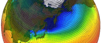
11 |
12 | 
13 | :::
14 | :::
15 | ::: {.fragment .fade-in}
16 | Data processing
17 |
18 | ::: {layout="[-30, 40, -30]" layout-valign="center"}
19 | 
20 | :::
21 |
22 | :::
23 | ::: {.fragment .fade-in}
24 | Experiment support
25 |
26 | ::: {layout="[-10, 30, -3, 32, -10]" layout-valign="center"}
27 | 
28 |
29 | 
30 | :::
31 |
32 | :::
33 |
34 | :::
35 |
36 | :::{.column}
37 | :::
38 | ::::
39 |
40 | {.absolute top=25% right=0% height=50%}
41 |
42 |
43 | ::: {.attribution}
44 | VLA Telescope by NROA under public domain
45 | CTD Bottles by WHOI under public domain\
46 | Keeling Curve by Scripps under public domain\
47 | Dawn HPC by Joe Bishop with permission\
48 | Climate simulation by NSF under public domain\
49 | :::
50 |
51 |
52 | ::: {.notes}
53 | * Data processing - FFT, averaging, etc.
54 | * Will inevetable be reused - making it good makes your life easier.
55 | * Software should be valued more than it is.\
56 | At time of writing there isn't pressure to write well.\
57 | This is not a good long-term strategy, however.
58 | :::
59 |
60 |
61 | ## Why does this matter? {.smaller}
62 | {.absolute top=12.5% right=15% width=70%}
63 |
64 |
65 | ## Why does this matter? {.smaller}
66 |
67 | More widely than publishing papers, code is used in control and decision making:
68 |
69 | :::: {.columns}
70 | ::: {.column width="60%"}
71 | \
72 |
73 | - Weather forecasting
74 | - Climate policy
75 | - Disease modelling (e.g. Covid)
76 | - Satellites and spacecraft[^*]
77 | - Medical Equipment
78 |
79 | \
80 |
81 | Your code (or its derivatives) may well move from research to operational one day.
82 |
83 | :::
84 | ::::
85 |
86 | {.absolute top=20% right=0% width=35%}
87 |
88 | [^*]: If possible to be even more awesome, it was MH [who first coined the term _"Software Engineering"_](https://www.computer.org/publications/tech-news/events/what-to-know-about-the-scientist-who-invented-the-term-software-engineering).]
89 |
90 | ::: {.attribution}
91 | Margaret Hamilton and the Apollo XI by NASA under public domain
92 | :::
93 |
94 |
95 | ## Why does this matter?^[For more details I highly recommend the [Writing Clean Scientific Software](https://www.youtube.com/watch?v=Q6Ksu_uX3bc) Webinar [@Murphy_2023]] {.smaller}
96 |
97 | :::: {.columns}
98 | ::: {.column width="50%"}
99 | ```python
100 | def calc_p(n,t):
101 | return n*1.380649e-23*t
102 | data = np.genfromtxt("mydata.csv")
103 | p = calc_p(data[0,:],data[1,:]+273.15)
104 | print(np.sum(p)/len(p))
105 | ```
106 | What does this code do?
107 | :::
108 | ::: {.column}
109 | ::: {.fragment .fade-in}
110 | ```python
111 | # Boltzmann Constant and 0 Kelvin
112 | Kb = 1.380649e-23
113 | T0 = 273.15
114 |
115 | def calc_pres(n, t):
116 | """
117 | Calculate pressure using ideal gas law p = nkT
118 |
119 | Parameters:
120 | n : array of number densities of molecules [N m-3]
121 | t : array of temperatures in [K]
122 | Returns:
123 | array of pressures [Pa]
124 | """
125 | return n * Kb * t
126 |
127 |
128 | # Read in data from file and convert T from [oC] to [K]
129 | data = np.genfromtxt("mydata.csv")
130 | n = data[0, :]
131 | temp = data[1, :] + T0
132 |
133 | # Calculate pressure, average, and print
134 | pres = calc_pres(n, temp)
135 | pres_av = np.sum(pres) / len(pres)
136 | print(pres_av)
137 |
138 | ```
139 | :::
140 | :::
141 | ::::
142 |
143 |
144 |
--------------------------------------------------------------------------------
/exercises/01_base_code/README.md:
--------------------------------------------------------------------------------
1 | # Exercise 1 - Setup and virtual environments
2 |
3 | Software environments are an important concept in development and deployment.
4 | They allow us to:
5 |
6 | - Control dependencies
7 | - Avoid system pollution through isolation
8 | - Allow different versions for different projects
9 | - Facilitate reproducibility - set specific versions
10 |
11 | For more information see the
12 | [Real Python article](https://realpython.com/python-virtual-environments-a-primer/)
13 | on virtual environments.
14 |
15 |
16 | ## First impressions
17 |
18 | Take a look at the files in this folder, opening the code in your preferred text editor.
19 |
20 | Note the package imports at the top of the script.
21 |
22 |
23 | ## Virtual environments
24 |
25 | Python has inbuilt support for creating isolated virtual environments through
26 | [`venv`](https://docs.python.org/3/library/venv.html).
27 |
28 | Set up a virtual environment and activate it:
29 |
30 | > [!NOTE]
31 | > It may be useful to place this a couple of directories higher under `/` or
32 | > `/exercises/` as it will be used for all exercises in the workshop.
33 |
34 | Unix/macOS:
35 | ```bash
36 | python3 -m venv rse-venv
37 | source rse-venv/bin/activate
38 | ```
39 | Windows Powershell:
40 | ```powershell
41 | python -m venv rse-venv
42 | rse-venv\Scripts\Activate.ps1
43 | ```
44 | Windows cmd.exe
45 | ```shell
46 | python -m venv rse-venv
47 | rse-venv\Scripts\activate.bat
48 | ```
49 |
50 | You will see that your command prompt is now preceded by `(rse-venv)` indicating
51 | that you are working in the virtual environment.
52 |
53 | To deactivate the environment use the `deactivate` command.
54 | You can always re-enter it later by running the activate script again.
55 |
56 | You will see that a directory `rse-venv/` has been created into which pip will install
57 | packages.
58 | To remove the venv (and any installed packages) we delete this directory with
59 | `rm -r rse-venv` on Unix, or `rmdir /s rse-venv` on Windows.
60 |
61 |
62 | ## Installing dependencies
63 |
64 | ### Manually
65 |
66 | You can now install the required dependencies into this environment using pip:
67 |
68 | ```bash
69 | pip install numpy matplotlib ...
70 | ```
71 | Once the dependencies are installed try to run the code:
72 |
73 | ```bash
74 | python3 geo.py
75 | ```
76 | for the geoscience code, or
77 | ```bash
78 | python3 astro.py
79 | ```
80 | for the astrophysics code.
81 |
82 | Does everything work as you expected or are there some unexpected dependencies required
83 | e.g. `netcdf4`?
84 |
85 | ### From a requirements file
86 |
87 | Installing dependencies manually one-at-a-time is tedious and a process of
88 | trial-and-error.
89 |
90 | Instead the author of the software should provide a list of all the dependencies
91 | required for running their code.
92 | In Python this is often done in a `requirements.txt` file that can be installed in
93 | one go:
94 |
95 | ```bash
96 | pip install -r requirements.txt
97 | ```
98 |
99 |
100 | ## Running the code
101 |
102 | You can now run the code from the command line using:
103 |
104 | ```
105 | python3 geo.py
106 | ```
107 | for the geoscience code, or
108 | ```bash
109 | python3 astro.py
110 | ```
111 | for the astrophysics code.
112 |
113 | Once you have done this take a moment to inspect the outputs.
114 | Did it do what you were expecting it to based on reading it beforehand?
115 |
116 |
117 | ## Finishing
118 |
119 | You can now move on to exercise two in the adjacent folder.
120 | Keep your virtual environment active as you will be re-using it!
121 |
122 |
123 | ## Other languages
124 |
125 | There are various other tools available to manage environments and dependencies in
126 | other languages:
127 |
128 | - Python and more - conda
129 | - C, C++, Fortran:
130 | - Module environments
131 | - Spack
132 | - Rust - cargo
133 | - Julia - Pkg environments
134 | - R - renv
135 |
136 |
137 | ## Further reading
138 |
139 | Providing a list of dependencies (e.g. `requirements.txt` file) should be a bare
140 | minimum when distributing software.
141 |
142 | As a project grows it is better to look at proper _software packaging_ to make your code
143 | easy for users to install, robust and reproducible, and portable to different systems.
144 | This is beyond the scope of today's workshop, however.
145 |
146 | You can read about packaging for Python in the
147 | [Python Packaging User Guide](https://packaging.python.org).
148 | This enables the project to be installed via pip, and can be achieved for simple
149 | projects by the inclusion of a `pyproject.toml` file.
150 |
151 | For other languages/projects there are a variety of packaging tools designed to help
152 | streamline the packaging and distribution process.
153 |
--------------------------------------------------------------------------------
/slides/_readme_license.qmd:
--------------------------------------------------------------------------------
1 | # READMEs, Licenses, and other files
2 |
3 |
4 |
5 | ## READMEs {.smaller}
6 |
7 | - First point of contact for a new user/contributor with the code repository
8 | - Should give essential information on
9 | - what this software is
10 | - what it's for
11 | - how to get started
12 | - In the best case it also tells you
13 | - who built/is building this
14 | - how to contribute
15 | - how to reuse
16 | - Usually written in [Markdown](https://www.markdownguide.org/) as `README.md`
17 | - See [makeareadme.com](https://www.makeareadme.com/) and [readme.so](https://readme.so/)
18 | for detailed information, examples, and tools
19 |
20 |
21 | ## Recommended README Content {.smaller}
22 |
23 | :::: {.columns style="font-size: 80%;"}
24 | ::: {.column width=47.5%}
25 | #### Essential:
26 |
27 | - Name
28 | - Overview of software
29 | - Install and build instructions
30 | - Usage/getting-started instructions (incl. simple example)
31 | - Documentation and Support: User Guide/Website/Help/Discussion forum
32 | - Information about contributing
33 | - Authors and Acknowledgment
34 | - License information
35 | - Known Issues
36 |
37 | :::
38 | ::: {.column width=5%}
39 | :::
40 | ::: {.column width=47.5%}
41 | #### Nice to have:
42 |
43 | - References to key papers/materials
44 | - Badges
45 | - Examples
46 | - Link to online docs
47 | - List of users
48 | - FAQ
49 | - See [readme.so/](https://readme.so) for a longer list
50 |
51 | :::
52 | ::::
53 |
54 |
55 |
56 | ## License {.smaller}
57 |
58 | All public codes should have a license attached!
59 |
60 | - `LICENSE` file in the main directory
61 | - Protect ownership
62 | - Limit liability
63 | - Clarify what can be done with the code
64 |
65 | The right selection may depend on your organisation and/or funder.
66 |
67 | See [choosealicense.com](https://choosealicense.com/) for more information.
68 |
69 | GitHub and GitLab contain helpers to create popular licenses.
70 |
71 |
72 | ## Types of Licenses {.smaller}
73 |
74 | - Public Domain, Permissive, Copyleft
75 |
76 | 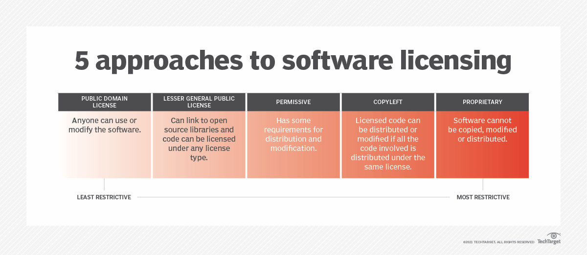{width=80% fig-align="center"}
77 |
78 | ::: {.attribution}
79 | License guide by [TechTarget](https://www.techtarget.com/searchcio/definition/software-license) under fair use
80 | :::
81 |
82 |
83 | ## How to choose a license {.smaller}
84 |
85 | :::: {.columns}
86 | ::: {.column width="70%"}
87 | - [https://choosealicense.com/licenses/](https://choosealicense.com/licenses/)
88 | - Permissive licenses:
89 | - Apache License 2.0
90 | - MIT License
91 | - Copyleft:
92 | - Means that copy/adaption has to use the same license
93 | - GNU General Public License v3.0
94 | :::
95 |
96 | ::: {.column}
97 | {.absolute top=12.5% right=5% width=20%}
98 | {.absolute top=35% right=10% width=20%}
99 | {.absolute top=70% right=5% width=20%}
100 | :::
101 | ::::
102 |
103 | ::: {.attribution}
104 | GPL3 image is in the Public Domain\
105 | MIT logo is in the Public Domain\
106 | Apache License image by Apache Software Foundation under Apache License 2.0
107 | :::
108 |
109 |
110 | ## Example: MIT License {.smaller}
111 |
112 | ```
113 | Copyright
114 |
115 | Permission is hereby granted, free of charge, to any person obtaining a copy of this software and associated documentation files (the “Software”), to deal in the Software without restriction, including without limitation the rights to use, copy, modify, merge, publish, distribute, sublicense, and/or sell copies of the Software, and to permit persons to whom the Software is furnished to do so, subject to the following conditions:
116 |
117 | The above copyright notice and this permission notice shall be included in all copies or substantial portions of the Software.
118 |
119 | THE SOFTWARE IS PROVIDED “AS IS”, WITHOUT WARRANTY OF ANY KIND, EXPRESS OR IMPLIED, INCLUDING BUT NOT LIMITED TO THE WARRANTIES OF MERCHANTABILITY, FITNESS FOR A PARTICULAR PURPOSE AND NONINFRINGEMENT. IN NO EVENT SHALL THE AUTHORS OR COPYRIGHT HOLDERS BE LIABLE FOR ANY CLAIM, DAMAGES OR OTHER LIABILITY, WHETHER IN AN ACTION OF CONTRACT, TORT OR OTHERWISE, ARISING FROM, OUT OF OR IN CONNECTION WITH THE SOFTWARE OR THE USE OR OTHER DEALINGS IN THE SOFTWARE.
120 | ```
121 |
122 | ## Add a license in Github {.smaller}
123 |
124 | {width=80% fig-align="center"}
125 |
126 | ## Add a license in Gitlab {.smaller}
127 |
128 | {width=80% fig-align="center"}
129 |
130 |
131 |
132 |
133 | ## Other potential files in your repository {.smaller}
134 |
135 | - CONTRIBUTING.md
136 | - CITATION.cff
137 | - CODE_OF_CONDUCT.md
138 | - CHANGES.md
139 |
140 |
141 |
--------------------------------------------------------------------------------
/slides/_formatting.qmd:
--------------------------------------------------------------------------------
1 | # PEP8 and Formatting
2 |
3 |
4 |
5 |
6 |
7 | ## Python PEPs {.smaller}
8 |
9 | [Python Enhancement Proposals](https://peps.python.org/)
10 |
11 | - Technical documentation for the python community
12 | - Guidelines, standards, and best-practice
13 |
14 | Relevant to us today are:
15 |
16 | * PEP8 - Python Style Guide [@PEP8]
17 | * PEP257 - Docstring Conventions [@PEP257]
18 | * PEP621 - Packaging [@PEP621]
19 |
20 |
21 |
22 |
23 |
24 | ## PEP8 & Formatting {.smaller}
25 |
26 | > _“Readability counts”_\
27 | > - Tim Peters in the [Zen of Python](https://peps.python.org/pep-0020/)
28 |
29 | By ensuring code aligns with PEP8 we:
30 |
31 | - standardise style,
32 | - conform to best-practices, and
33 | - improve code readability to
34 | - make code easier to share, and
35 | - reduce misinterpretation.
36 |
37 | ::: {.fragment}
38 | "But I don't have time to read and memorise all of this..."
39 | :::
40 |
41 |
42 |
43 |
44 |
45 | ## PEP8 & Formatting - Ruff {.smaller}
46 |
47 | {.absolute top=20% right=20% height=30%}
48 |
49 | Ruff [@ruff] - [docs.astral.sh/ruff](https://docs.astral.sh/ruff/)
50 |
51 | - a PEP 8 compliant formatter
52 | - Strict subset of PEP8
53 | - _"Opinionated so you don't have to be."_
54 | - For full details see [style guide](https://docs.astral.sh/ruff/formatter/#style-guide)
55 | - [Try online](https://play.ruff.rs/?secondary=Format)
56 |
57 | ::: {.panel-tabset}
58 |
59 | ### Linux/macOS
60 |
61 | ``` default
62 | (rse-venv) $ pip install ruff
63 | (rse-venv) $ ruff format myfile.py
64 | (rse-venv) $ ruff format mydirectory/
65 | ```
66 |
67 | ### Windows
68 |
69 | ```default
70 | (rse-venv) PS> pip install ruff
71 | (rse-venv) PS> ruff format myfile.py
72 | (rse-venv) PS> ruff format mydirectory/
73 | ```
74 | :::
75 |
76 | ::: {.notes}
77 | May look odd at first, but you soon get used to it.\
78 | Makes life so much easier after a while.
79 | :::
80 |
81 |
82 |
83 |
84 |
85 | ## PEP8 & Formatting - Example {.smaller}
86 |
87 | :::: {.columns}
88 | ::: {.column width="50%"}
89 | ```python
90 | def long_func(x, param_one, param_two=[], param_three=24, param_four=None,
91 | param_five="Empty Report", param_six=123456):
92 |
93 |
94 | val = 12*16 +(24) -10*param_one + param_six
95 |
96 | if x > 5:
97 |
98 | print("x is greater than 5")
99 |
100 |
101 | else:
102 | print("x is less than or equal to 5")
103 |
104 |
105 | if param_four:
106 | print(param_five)
107 |
108 |
109 |
110 | print('You have called long_func.')
111 | print("This function has several params.")
112 |
113 | param_2.append(x*val)
114 | return param_2
115 |
116 | ```
117 | :::
118 | ::: {.column}
119 | ```python
120 | def long_func(
121 | x,
122 | param_one,
123 | param_two=[],
124 | param_three=24,
125 | param_four=None,
126 | param_five="Empty Report",
127 | param_six=123456,
128 | ):
129 | val = 12 * 16 + (24) - 10 * param_one + param_six
130 |
131 | if x > 5:
132 | print("x is greater than 5")
133 |
134 | else:
135 | print("x is less than or equal to 5")
136 |
137 | if param_four:
138 | print(param_five)
139 |
140 | print("You have called long_func.")
141 | print("This function has several params.")
142 |
143 | param_2.append(x * val)
144 | return param_2
145 | ```
146 | :::
147 | ::::
148 |
149 |
150 |
151 |
152 |
153 | ## PEP8 & Formatting - Ruff {.smaller}
154 |
155 | - Also runs on jupyter notebooks.
156 |
157 | - Highly configurable via configuration files.
158 |
159 | - I suggest incorporating into your projects now
160 | - Widely-used standard^[[Who's Using Ruff?](https://github.com/astral-sh/ruff#whos-using-ruff)]
161 | - Plugins/lsp available for many editors.
162 | - Well suited to incorporation into continuous integration through workflows and git hooks.
163 |
164 |
165 |
166 |
167 |
168 | ## Other languages {.smaller}
169 |
170 | Similar formatting tools exist for other languages:
171 |
172 | - Python - [ruff](https://docs.astral.sh/ruff/) or
173 | [black](https://black.readthedocs.io/en/stable/index.html)
174 | - C and C++ - [clang-format](https://clang.llvm.org/docs/ClangFormat.html)
175 | - Fortran - [fortitude](https://github.com/PlasmaFAIR/fortitude) (in development)
176 | - Rust - [rustfmt](https://github.com/rust-lang/rustfmt)
177 | - Julia - [JuliaFormatter.jl](https://github.com/domluna/JuliaFormatter.jl)
178 | - R - [styler](https://github.com/r-lib/styler) or [Air](https://github.com/posit-dev/air)
179 |
180 |
181 |
182 |
183 |
184 | ## Exercise 2 {.smaller}
185 |
186 | Go to exercise 2 and:
187 |
188 | - install ruff
189 | - run `ruff format` on the Python code.
190 | - examine the output
191 | - Is it more readable?
192 | - Is there any aspect of the formatting style you find unintuitive?
193 | - See `exercises/02_formatting/README.md` for more detailed instructions.
194 |
195 |
196 |
197 |
--------------------------------------------------------------------------------
/exercises/03_linting/README.md:
--------------------------------------------------------------------------------
1 | # Exercise 3 - Linting
2 |
3 | Beyond a consistent formatting style there are often various other ways in which code
4 | can be improved to conform to best practices or avoid certain bugs.
5 |
6 | Linting or static analysis uses tools to improve code quality.
7 | They are also a great way to learn better practices and new techniques.
8 |
9 | They also help save time and resources by checking code and identifying (some) runtime
10 | issues before execution.
11 |
12 |
13 | ## Run a linter over the code
14 |
15 | We will start by running the `ruff` linter over the code.
16 | Since we already installed ruff in exercise 1 to use its formatting tool there is no
17 | need to install anything new.
18 |
19 | To warm up take a look at the code in `long_func.py`.
20 | Can you spot anything wrong at a first glance?
21 |
22 | Run `ruff check` on the code and observe the warnings.
23 |
24 | ```bash
25 | ruff check long_func.py
26 | ```
27 |
28 | > [!TIP]
29 | > When re-running ruff to check fixes you may find it useful to use the
30 | > `--output-format=concise` flag to reduce printed output.
31 |
32 |
33 |
34 | Click here for the explanation
35 |
36 | ```console
37 | (rse-venv) $ ruff check long_func.py
38 | long_func.py:4:5: ARG001 Unused function argument: `param_two`
39 | long_func.py:4:15: B006 Do not use mutable data structures for argument defaults
40 | long_func.py:5:5: ARG001 Unused function argument: `param_three`
41 | long_func.py:24:5: F821 Undefined name `param_2`
42 | long_func.py:25:12: F821 Undefined name `param_2`
43 | Found 5 errors.
44 |
45 | (rse-venv) $
46 | ```
47 |
48 | We can see from the output that there is a mismatch in name between `param_two` and
49 | `param_2` that would have caused a runtime error.
50 |
51 | We can also see that there is some housekeeping to be carried out to remove unused
52 | variables and keep things clean.
53 |
54 | Finally, there is a somewhat more cryptic `B006 Do not use mutable data structures`.
55 | To understand this we can ask ruff to provide some explanation by running
56 |
57 |
58 |
59 | We can now proceed to running ruff on the full code:
60 |
61 | ```
62 | ruff check geo.py
63 | ```
64 | or
65 | ```
66 | ruff check astro.py
67 | ```
68 |
69 |
70 | ## Improving the code
71 |
72 | Open the source code in your text editor and modifiy it to fix
73 | the linting errors:
74 |
75 | - Try and deal with: `F401` unused imports, `I001` unsorted imports,
76 | `B006` dangerous default, and `D202` Blank lines
77 | - For a challenge try and fix: `RUF059` unused unpack
78 | - In `geo.py` there is also `B904` try exceptions
79 | - In `astro.py` there is also `RUF059` unused unpack, `A001` shadowing, and
80 | `PLR1714` merging comparisons (`F841` we will cover in exercise 5).
81 |
82 | Extensions:
83 |
84 | - explore autofixes using the `--fix` flag
85 | - explore rules in development using the `--preview` flag
86 | - try and add linting to your preferred text editor or IDE
87 |
88 | As you work through the errors do you understand how adressing them has improved
89 | your code?
90 |
91 | Have you learnt anything new from fixing them?
92 |
93 | > [!TIP]
94 | > Don't forget to re-run `ruff format` after you have finished editing your code to keep
95 | > the formatting rules enforced.
96 |
97 |
98 | ## Extension exercises
99 |
100 | - See if you can install some form of ruff (or another linter) in your text editor/IDE
101 | as a language server to highlight mistakes whilst you write! See [ruff editor integration docs](https://docs.astral.sh/ruff/editors/setup/).
102 | - If there are any warnings you are going to ignore, see if you can
103 | [supress them](https://docs.astral.sh/ruff/linter/#error-suppression)
104 | so they don't clutter up the report.
105 | - Explore the option of
106 | [altering the configuration settings](https://docs.astral.sh/ruff/configuration/)
107 | in the configuration file.
108 | - Explore the different rulesets available in the
109 | [ruff rules documentation](https://docs.astral.sh/ruff/rules/).
110 |
111 |
112 | ## Configuration
113 |
114 | The default set of linting rules for ruff is quite simple.
115 |
116 | The ruleset to be applied can be configured in a `ruff.toml` file, as we do in this project,
117 | or `pyproject.toml` for packaged code.
118 | For full details see the [ruff configuration documentation](https://docs.astral.sh/ruff/configuration/).
119 |
120 | Details of the different rules and rulesets that can be selected can be found in the
121 | [ruff rules documentation](https://docs.astral.sh/ruff/rules/).
122 |
123 | In this project we use a `ruff.toml` file at the root of the repository.
124 | Take a look and make some changes in preparation for the next
125 | sections:
126 |
127 | - We will add the entire `"D"` (pydocstyle) ruleset by adding it to the `select` list.
128 | - We will stop ignoring:
129 | - `"PLR2004"` (magic number comparisons),
130 | - `"E501"` (line length), and
131 | - `"E741"` (ambiguous name).
132 | by removing them from the `ignore` list.
133 | - We will add `"D417"` (Missing argument description) by adding it to the
134 | `extend-select` list.
135 |
136 |
137 | ## Other languages
138 |
139 | Similar tools for linting and static analysis exist for other languages:
140 |
141 | - C and C++ - [clang-tidy](https://clang.llvm.org/extra/clang-tidy/) and
142 | [cppcheck](https://cpp-linter.github.io/)
143 | - Fortran - [fortitude](https://github.com/PlasmaFAIR/fortitude)
144 | - Rust - [clippy](https://doc.rust-lang.org/clippy/)
145 | - R - [lintr](https://lintr.r-lib.org/)
146 |
147 | More generally see [this list of static analysis tools](https://github.com/analysis-tools-dev/static-analysis).
148 |
--------------------------------------------------------------------------------
/slides/_venv.qmd:
--------------------------------------------------------------------------------
1 | # Virtual Environments
2 |
3 | ## Virtual Environments {.smaller}
4 |
5 | \
6 |
7 | :::: {.columns}
8 | ::: {.column width="50%"}
9 | #### What?
10 |
11 | - A self-contained Python environment
12 | - Packages installed in a local folder
13 | - Advised to use on a per-project basis
14 |
15 | :::
16 | ::: {.column}
17 | #### Why?
18 |
19 | - Avoid system pollution through isolation
20 | - Allow different versions for different projects
21 | - Reproducibility - set versions
22 |
23 | :::
24 | ::::
25 |
26 | ::: aside
27 | For more information see the [Real Python article](https://realpython.com/python-virtual-environments-a-primer/)
28 | on virtual environments.
29 | :::
30 |
31 |
32 |
33 |
34 | ## Virtual Environments - `venv` {.smaller}
35 |
36 | Python has inbuilt support for creating isolated virtual environments through
37 | [`venv`](https://docs.python.org/3/library/venv.html).
38 |
39 | \
40 |
41 | ::: {.panel-tabset}
42 |
43 | ### Linux/macOS
44 |
45 | ```default
46 | $ python3 -m venv rse-venv
47 | $ source rse-venv/bin/activate
48 | (rse-venv) $ pip install
49 | (rse-venv) $ deactivate
50 | $
51 |
52 | ```
53 |
54 | ### Windows Powershell
55 |
56 | ```default
57 | PS> python -m venv rse-venv
58 | PS> rse-venv\Scripts\Activate.ps1
59 | (rse-venv) PS> pip install
60 | (rse-venv) PS> deactivate
61 | PS>
62 | ```
63 |
64 | ### Windows cmd.exe
65 |
66 | ```default
67 | C:\> python -m venv rse-venv
68 | C:\> rse-venv\Scripts\activate.bat
69 | (rse-venv) C:\> pip install
70 | (rse-venv) C:\> deactivate
71 | C:\>
72 | ```
73 |
74 | :::
75 |
76 | \
77 |
78 | You will see that a directory `rse-venv/` has been created.\
79 | Pip will install dependencies into this directory.\
80 | To remove the venv we delete this directory with `rm -r rse-venv` on Unix, or
81 | `rmdir /s rse-venv` on Windows.
82 |
83 |
84 |
85 |
86 |
87 | ## Other Languages {.smaller}
88 |
89 | There are various other tools available to manage dependencies:
90 |
91 | - Python and more - conda
92 | - C, C++, Fortran:
93 | - Module environments
94 | - Spack
95 | - Rust - cargo
96 | - Julia - Pkg environments
97 | - R - renv
98 |
99 |
100 |
101 |
102 |
103 | ## Exercise 1 {.smaller}
104 |
105 | ::: {.panel-tabset}
106 |
107 | ### Geoscience
108 |
109 | Scenario: you have just finished some simulations with a climate model that should
110 | improve precipitation modelling and have the output data as a netCDF file.
111 |
112 | You know that your colleague has produced relevant figures and analysis before, so ask
113 | them for a copy of their code (yay, reuse :+1:).
114 |
115 | Go to exercise 1 and examine the code in `geo.py`.
116 |
117 | ### Astrophysics
118 |
119 | Scenario: you have just finished preparing a new stellar dataset in a csv file and want
120 | to visualise the data to see what it tells you.
121 |
122 | You know that your colleague has produced relevant figures and analysis for similar data
123 | before, so ask them for a copy of their code (yay, reuse :+1:).
124 |
125 | Go to exercise 1 and examine the code in `astro.py`
126 |
127 | :::
128 |
129 | - Create and load a virtual environment
130 | - Install the necessary dependencies
131 | - Run the code - does it do what you thought?
132 | - Deactivate the environment
133 |
134 |
135 |
136 |
137 |
138 |
139 | ## Basic packaging concepts {.smaller}
140 |
141 | Code/software will often have several dependencies required to run.
142 |
143 | Provide a record of these to users to save time and errors when installing.
144 |
145 | \
146 |
147 | :::: {.columns}
148 | ::: {.column width="70%"}
149 |
150 | Recorded in a `requirements.txt` file:
151 |
152 | - list required packages to be installed by pip
153 | - version constraints
154 | - typically specify top-level^[We can pin everything using `pip freeze`, but there are better ways to do this.]
155 |
156 | :::
157 | ::: {.column width="30%"}
158 | `requirements.txt`
159 | ```default
160 | netcdf4
161 | xarray
162 | scipy==1.13.1
163 | numpy<2.0
164 | cartopy
165 | ```
166 | :::
167 | ::::
168 |
169 | \
170 |
171 |
172 | ```default
173 | (rse-venv) $ pip install -r requirements.txt
174 | ```
175 |
176 |
177 | ::: aside
178 | We can improve and streamline this process even further through packaging, but this is
179 | beyond the scope of this discussion.
180 | :::
181 |
182 |
183 |
184 |
185 |
186 | ## Exercise 1 revisited {.smaller}
187 |
188 | ::: {.panel-tabset}
189 |
190 | ### Geoscience
191 |
192 | Scenario: you have just finished some simulations with a climate model that should
193 | improve precipitation modelling and have the output data as a netCDF file.
194 |
195 | You know that your colleague has produced relevant figures and analysis before, so ask
196 | them for a copy of their code (yay, reuse :+1:).
197 |
198 | Go to exercise 1 and examine the code in `geo.py`.
199 |
200 | ### Astrophysics
201 |
202 | Scenario: you have just finished preparing a new stellar dataset in a csv file and want
203 | to visualise the data to see what it tells you.
204 |
205 | You know that your colleague has produced relevant figures and analysis for similar data
206 | before, so ask them for a copy of their code (yay, reuse :+1:).
207 |
208 | Go to exercise 1 and examine the code in `astro.py`
209 |
210 | :::
211 |
212 | - Create and load a virtual environment
213 | - Install the requirements from the supplied `requirements.txt`
214 | - Run the code - does it do what you thought?
215 | - Deactivate the environment
216 |
217 |
218 |
219 |
--------------------------------------------------------------------------------
/slides/_naming_magic_numbers.qmd:
--------------------------------------------------------------------------------
1 |
2 | # Naming Clarity and Magic Numbers
3 |
4 |
5 | ## Naming for clarity {.smaller}
6 |
7 | \
8 |
9 | It may seem inconsequential, but carefully naming variables and methods can greatly
10 | improve the readability of code.
11 |
12 | \
13 |
14 | Since _"code is read more than it is run"_ this is important for future you, but also
15 | for anyone you collaborate with or who might use your code in future.
16 |
17 | \
18 |
19 | It helps to make code self-documenting, reducing future bugs due to misunderstandings.
20 |
21 | \
22 |
23 | Here we cover some key considerations when writing code.
24 |
25 |
26 |
27 | ## Naming for clarity {.smaller}
28 |
29 | ::: {.incremental}
30 | - Show the intention -- how will someone else (future you) read it?
31 | - Use readable, pronounceable, memorable, and searchable names:
32 | ```
33 | ms --> mass
34 | chclt --> chocolate
35 | stm --> stem
36 | ```
37 | avoid abbreviations and single letters unless commonly used
38 | - Employ concept consistency \
39 | e.g. only one of `get_`, `retrive_`, `fetch_` in the code base
40 | - Describe content rather than storage type \
41 | Use plurals to indicate groups \
42 | Name booleans using prefixes like `is_`, `has_`, `can_` and avoid negations like `not_`:
43 | ```
44 | array --> dogs float_or_int --> returns_int
45 | age_int --> age not_plant --> is_plant
46 | country_set --> countries sidekick --> has_sidekick
47 | ```
48 | :::
49 |
50 |
51 |
52 | ## Explaining Variables {.smaller}
53 |
54 | Without explaining variable: \
55 |
56 | ```python
57 |
58 | def calculate_fare(age):
59 | if (age < 14):
60 | return 3
61 | ...
62 | ```
63 |
64 | \
65 |
66 | With explaining variable: \
67 |
68 | ```python
69 |
70 | def calculate_fare(age):
71 | is_child = age < 14
72 | if (is_child):
73 | return 3
74 | ...
75 | ```
76 |
77 |
78 |
79 | ## Explaining Variables {.smaller}
80 |
81 | Without an explaining variable, it is hard to see what this code is doing:
82 |
83 | ```python
84 | import re
85 |
86 | re.search("^\\+?[1-9][0-9]{7,14}$", "Sophie: CV56 9PQ, +12223334444")
87 | ```
88 |
89 | \
90 |
91 | ::: {.fragment}
92 | With explaining variables it is easier to see the intention. \
93 | The code is more self-documenting.
94 |
95 | ```python
96 | import re
97 |
98 | phone_number_regex = "^\\+?[1-9][0-9]{7,14}$"
99 | re.search(phone_number_regex, "Sophie: CV56 9PQ, +12223334444")
100 | ```
101 | :::
102 |
103 |
104 |
105 | ## Magic Numbers {.smaller}
106 |
107 | Numbers in code that are not immediately obvious.
108 |
109 | - Hard to read
110 | - Hard to maintain
111 | - Hard to adapt
112 |
113 | Instead:
114 |
115 | - Name a variable conveying meaning
116 | - Set to a constant
117 | - Use a comment to explain
118 |
119 | {.absolute top=33% right=0% height=33%}
120 |
121 | ::: {.attribution}
122 | numberwang by Mitchell and Webb under fair use
123 | :::
124 |
125 |
126 |
127 | ## Handling Magic Numbers {.smaller}
128 |
129 | :::: {.columns}
130 |
131 | ::: {.column width="50%"}
132 | :::{ style="font-size: 85%;"}
133 | ```python {code-line-numbers=True}
134 | """Module implementing pendulum equations."""
135 | import numpy as np
136 |
137 | def get_period(l):
138 | """..."""
139 | return 2.0 * np.pi * np.sqrt(l / 9.81)
140 |
141 | def max_height(l, theta):
142 | """..."""
143 | return l * np.cos(theta)
144 |
145 | def max_speed(l, theta):
146 | """..."""
147 | return np.sqrt(2.0 * 9.81 * max_height(l, theta))
148 |
149 | def energy(m, l, theta):
150 | """..."""
151 | return m * 9.81 * max_height(l, theta)
152 |
153 | def check_small_angle(theta):
154 | """..."""
155 | if theta <= np.pi / 1800.0:
156 | return True
157 | return False
158 |
159 | def beats_per_minute(l):
160 | """..."""
161 | return 60.0 / get_period(l)
162 |
163 |
164 |
165 |
166 | ```
167 | :::
168 | :::
169 | ::: {.column}
170 | :::{ style="font-size: 85%;"}
171 | ```python {code-line-numbers="|4,8,16,20|22,24|30,31"}
172 | """Module implementing pendulum equations."""
173 | import numpy as np
174 |
175 | GRAV = 9.81
176 |
177 | def get_period(l):
178 | """..."""
179 | return 2.0 * np.pi * np.sqrt(l / GRAV)
180 |
181 | def max_height(l, theta):
182 | """..."""
183 | return l * np.cos(theta)
184 |
185 | def max_speed(l, theta):
186 | """..."""
187 | return np.sqrt(2.0 * GRAV * max_height(l, theta))
188 |
189 | def energy(m, l, theta):
190 | """..."""
191 | return m * GRAV * max_height(l, theta)
192 |
193 | def check_small_angle(theta, small_ang=np.pi/1800.0):
194 | """..."""
195 | if theta <= small_ang:
196 | return True
197 | return False
198 |
199 | def beats_per_minute(l):
200 | """..."""
201 | # Divide 60 seconds by period [s] for beats per minute
202 | return 60.0 / get_period(l)
203 | ```
204 | :::
205 | :::
206 | ::::
207 |
208 |
209 |
210 |
211 | ## Exercise 5 {.smaller}
212 |
213 | Look through the code for method or variable names that could be improved or
214 | clarified and update them.^[Note: if you are using an IDE like Intellij or VSCode you can use automatic renaming.]
215 |
216 | Look through the code and identify any magic numbers.\
217 | Implement what you feel to be the best approach in each case.
218 |
219 |
220 | Does this make the code easier to follow?
221 |
222 | \
223 |
224 | ::: {style="font-size: 80%;"}
225 |
226 | Consider the following, can you find an example of each:
227 |
228 | :::: {.columns}
229 | ::: {.column width="65%"}
230 | - Show the intention -- how will someone else (future you) read it
231 | - Use readable, pronounceable, memorable, and searchable names
232 | - Keep it simple using technical terms where appropriate
233 | - Employ concept consistency in the code base
234 | :::
235 | ::: {.column width="35%"}
236 | - Describe content rather than type
237 | - Use plurals to indicate groups
238 | - Name booleans using prefixes
239 | - Use explaining variables
240 | :::
241 | ::::
242 |
243 | :::
244 |
245 |
246 |
--------------------------------------------------------------------------------
/slides/_linting.qmd:
--------------------------------------------------------------------------------
1 |
2 | # Static Analysis
3 |
4 |
5 |
6 | ## Static Analysis {.smaller}
7 |
8 | :::: {.columns}
9 | ::: {.column width="50%"}
10 | Beyond PEP8:
11 |
12 | - Improve code quality
13 | - Learn better practices
14 |
15 | Save time and resource:
16 |
17 | - Check code for issues without running
18 | :::
19 | ::: {.column width="50%"}
20 | There are various tools available:
21 |
22 | - ruff
23 | - Pylint
24 | - flake8
25 | - pycodestyle
26 | :::
27 | ::::
28 |
29 | \
30 |
31 | We will be using `ruff check` for static analysis, which we already installed as part
32 | of `ruff` in a previous exercise.
33 |
34 |
35 |
36 |
37 | ## Code Quality - `ruff check` {.smaller}
38 |
39 | :::: {.columns}
40 | ::: {.column width="50%"}
41 | ```python
42 | def long_func(
43 | x,
44 | param_one,
45 | param_two=[],
46 | param_three=24,
47 | param_four=None,
48 | param_five="Empty Report",
49 | param_six=123456,
50 | ):
51 | val = 12 * 16 + (24) - 10 * param_one + param_six
52 |
53 | if x > 5:
54 | print("x is greater than 5")
55 |
56 | else:
57 | print("x is less than or equal to 5")
58 |
59 | if param_four:
60 | print(param_five)
61 |
62 | print("You have called long_func.")
63 | print("This function has several params.")
64 |
65 | param_2.append(x * val)
66 | return param_2
67 | ```
68 | :::
69 | ::: {.column style="font-size: 75%;"}
70 | :::
71 | ::::
72 |
73 |
74 | ## Code Quality - `ruff check` {.smaller}
75 |
76 | :::: {.columns}
77 | ::: {.column width="50%"}
78 | ```python
79 | def long_func(
80 | x,
81 | param_one,
82 | param_two=[],
83 | param_three=24,
84 | param_four=None,
85 | param_five="Empty Report",
86 | param_six=123456,
87 | ):
88 | val = 12 * 16 + (24) - 10 * param_one + param_six
89 |
90 | if x > 5:
91 | print("x is greater than 5")
92 |
93 | else:
94 | print("x is less than or equal to 5")
95 |
96 | if param_four:
97 | print(param_five)
98 |
99 | print("You have called long_func.")
100 | print("This function has several params.")
101 |
102 | param_2.append(x * val)
103 | return param_2
104 | ```
105 | :::
106 | ::: {.column style="font-size: 75%;"}
107 | ```default
108 | (rse-venv) $ ruff check long_func.py
109 | long_func.py:4:5: ARG001 Unused function argument: `param_two`
110 | long_func.py:4:15: B006 Do not use mutable data structures for argument defaults
111 | long_func.py:5:5: ARG001 Unused function argument: `param_three`
112 | long_func.py:24:5: F821 Undefined name `param_2`
113 | long_func.py:25:12: F821 Undefined name `param_2`
114 | Found 5 errors.
115 |
116 | (rse-venv) $
117 |
118 | ```
119 | Note: \
120 | use the `--output-format=concise`
flag for this shortened output.
121 | :::
122 | ::::
123 |
124 | ::: {.notes}
125 | Caught a bug - param2\
126 | Caught unused variable param_three
127 | :::
128 |
129 |
130 | ## Code Quality - `ruff check` {.smaller}
131 |
132 | :::: {.columns}
133 | ::: {.column width="50%"}
134 | ```python
135 | def long_func(
136 | x,
137 | param_one,
138 | param_two=[],
139 | param_four=None,
140 | param_five="Empty Report",
141 | param_six=123456,
142 | ):
143 | val = 12 * 16 + (24) - 10 * param_one + param_six
144 |
145 | if x > 5:
146 | print("x is greater than 5")
147 |
148 | else:
149 | print("x is less than or equal to 5")
150 |
151 | if param_four:
152 | print(param_five)
153 |
154 | print("You have called long_func.")
155 | print("This function has several params.")
156 |
157 | param_two.append(x * val)
158 | return param_two
159 | ```
160 | :::
161 | ::: {.column style="font-size: 75%;"}
162 | ```default
163 | (rse-venv) $ ruff check long_func.py
164 | long_func.py:4:15: B006 Do not use mutable data structures for argument defaults
165 | Found 1 errors.
166 |
167 | (rse-venv) $
168 |
169 | ```
170 | \
171 | Use `ruff rule` to understand different rules:
172 | ```
173 | ruff rule B006
174 | ```
175 | will display the [docs for B006](https://docs.astral.sh/ruff/rules/mutable-argument-default/)
176 |
177 | :::
178 | ::::
179 |
180 | ::: {.notes}
181 | We now have runnable code!\
182 | :::
183 |
184 |
185 |
186 |
187 |
188 | ## IDE Integration {.smaller}
189 |
190 | - Catch issues before running ruff
191 | - Gradually coerces you to become a better programmer
192 | - See [ruff editor integration docs](https://docs.astral.sh/ruff/editors/setup/) for
193 | instructions on setup for:
194 | - Vim
195 | - pycharm
196 | - Sublime
197 | - VS Code
198 | - Emacs
199 |
200 |
201 |
202 |
203 |
204 | ## Other languages {.smaller}
205 |
206 | Similar tools for linting and static analysis exist for other languages:
207 |
208 | - C and C++ - [clang-tidy](https://clang.llvm.org/extra/clang-tidy/) and
209 | [cppcheck](https://cpp-linter.github.io/)
210 | - Fortran - [fortitude](https://github.com/PlasmaFAIR/fortitude)
211 | - Rust - [clippy](https://doc.rust-lang.org/clippy/)
212 | - R - [lintr](https://lintr.r-lib.org/)
213 |
214 | More generally see [this list of static analysis tools](https://github.com/analysis-tools-dev/static-analysis).
215 |
216 |
217 |
218 |
219 |
220 | ## Exercise 3 {.smaller}
221 |
222 | ::: {.panel-tabset}
223 |
224 | ### Geoscience
225 |
226 | Go to exercise 3 and:
227 |
228 | - run `ruff check` on `geo.py`
229 | - examine the report and try and address some of the issues.
230 | - Try and deal with: `F401` unused imports, `I001` unsorted imports,
231 | `B006` dangerous default, and `D202` Blank lines
232 | - For a challenge try and fix: `B904` try exceptions and `RUF059` unused unpack
233 |
234 | ### Astrophysics
235 |
236 | Go to exercise 3 and:
237 |
238 | - run `ruff check` on `astro.py`
239 | - examine the report and try and address some of the issues.
240 | - Try and deal with: `F401` unused imports, `I001` unsorted imports,
241 | `B006` dangerous default, and `D202` Blank lines
242 | - For a challenge try and fix: `A001` shadowing, and `PLR1714` merging comparisons.
243 | - Ignore `F841` for now as we will address it in a later exercise.
244 |
245 | :::
246 |
247 | Extensions:
248 |
249 | - explore autofixes using the `--fix` flag
250 | - explore rules in development using the `--preview` flag
251 | - try and add linting to your preferred text editor or IDE
252 |
253 |
254 |
255 |
256 | ## Configuration {.smaller}
257 |
258 | The default set of linting rules for ruff is quite simple.
259 |
260 | The ruleset to be applied can be configured in a `ruff.toml` file, as we do in this project,
261 | or `pyproject.toml` for packaged code. \
262 | For full details see the [ruff configuration documentation](https://docs.astral.sh/ruff/configuration/).
263 |
264 | Details of the different rules and rulesets that can be selected can be found in the
265 | [ruff rules documentation](https://docs.astral.sh/ruff/rules/).
266 |
267 | \
268 |
269 | Let's take a look and make some changes in preparation for the next
270 | sections:
271 |
272 | - We will add the entire `"D"` (pydocstyle) ruleset, extending to `D417`.
273 | - We will stop ignoring:
274 | - `"PLR2004"` (magic number comparisons) and
275 | - `"E501"` (line length).
276 | - `"E741"` (ambiguous name).
277 |
278 |
279 |
--------------------------------------------------------------------------------
/slides/rse-skills.qmd:
--------------------------------------------------------------------------------
1 | ---
2 | title: "RSE Skills"
3 | subtitle: "(in Python)"
4 |
5 | output-file: index
6 |
7 | format:
8 | revealjs:
9 | embed-resources: true
10 | slide-number: false
11 | chalkboard: false
12 | preview-links: auto
13 | history: false
14 | highlight-style: a11y
15 | code-overflow: wrap
16 | code-line-numbers: false
17 | logo: https://iccs.cam.ac.uk/sites/default/files/iccs_ucam_combined_reverse_colour.png
18 | theme: [dark, custom.scss]
19 | revealjs-plugins:
20 | - attribution
21 |
22 | authors:
23 | - name: Jack Atkinson
24 | orcid: 0000-0001-5001-4812
25 | affiliations:
26 | - ref: iccs
27 | affiliations:
28 | - id: iccs
29 | name: ICCS RSE Team
University of Cambridge
30 |
31 | date: "2025/11/28"
32 | bibliography: references.bib
33 | ---
34 |
35 | ## Precursors {.smaller .nostretch}
36 |
37 | :::: {.columns}
38 | ::: {.column width="65%"}
39 | #### Slides and Materials
40 |
41 | To access links or follow on your own device these slides can be found at:
42 | [jatkinson1000.github.io/rse-skills-workshop](https://jatkinson1000.github.io/rse-skills-workshop/)
43 |
44 | \
45 |
46 | All materials are available at:
47 |
48 | ::: {.column style="font-size: 95%;"}
49 |
50 | - [github.com/jatkinson1000/rse-skills-workshop](https://github.com/jatkinson1000/rse-skills-workshop)
51 | - [gitlab.com/jatkinson1000/rse-skills-workshop](https://gitlab.com/jatkinson1000/rse-skills-workshop)
52 | :::
53 | :::
54 | ::: {.column width="5%"}
55 | :::
56 | ::: {.column width="30%"}
57 |
58 | {{< fa solid person-chalkboard >}}:
59 | {{< qrcode https://github.com/jatkinson1000/rse-skills-workshop fkrycvbsgt width=150 height=150 >}}
60 |
61 | \
62 |
63 | {{< fa brands github >}}:
64 | {{< qrcode https://github.com/jatkinson1000/rse-skills-workshop qr7dekity9 width=150 height=150 >}}
65 |
66 | :::
67 | ::::
68 |
69 |
70 | ## Precursors {.smaller}
71 |
72 | :::: {.columns}
73 | ::: {.column width="45%"}
74 | #### Behaviour
75 |
76 | - Be nice ([Python code of conduct](https://www.python.org/psf/conduct/))
77 | - Ask questions whenever they arise.
78 | - Someone else is probably wondering the same thing.
79 | - We will make mistakes.
80 | - Not all of them will be intentional.
81 | :::
82 | ::: {.column width="5%"}
83 | :::
84 | ::: {.column width="45%"}
85 | #### Licensing
86 |
87 | Except where otherwise noted, these presentation materials are licensed under the Creative Commons
88 | [Attribution-NonCommercial 4.0 International](https://creativecommons.org/licenses/by-nc/4.0/legalcode) ([CC BY-NC 4.0](https://creativecommons.org/licenses/by-nc/4.0/)) License.
89 |
90 | {width=40% fig-align="center"}
91 |
92 | Vectors and icons by [SVG Repo](https://www.svgrepo.com)
93 | used under [CC0(1.0)](https://creativecommons.org/publicdomain/zero/1.0/deed.en)
94 | :::
95 | ::::
96 |
97 | ## Course structure {.smaller}
98 |
99 | :::: {.columns}
100 | ::: {.column width="45%"}
101 |
102 | - Why good SE matters in research
103 | - How to apply these everyday to write higher quality code
104 | - Core principles
105 | - Key tools
106 | - Useful techniques
107 |
108 | :::
109 |
110 | ::: {.column width="10%"}
111 | :::
112 |
113 | ::: {.column width="45%"}
114 |
115 | - Tooling for better research software
116 | - venv for virtual environments
117 | - formatting and linting - best practices
118 | - structuring code
119 | - Writing better research software
120 | - comments and docstrings
121 | - repository documentation - licenses, README
122 | - Other (naming, magic numbers,...)
123 |
124 | :::
125 | ::::
126 |
127 |
145 |
146 |
147 |
148 | {{< include _rse.qmd >}}
149 |
150 |
151 |
152 | {{< include _venv.qmd >}}
153 |
154 |
155 |
156 | {{< include _formatting.qmd >}}
157 |
158 |
159 |
160 | {{< include _linting.qmd >}}
161 |
162 |
163 |
164 | {{< include _naming_magic_numbers.qmd >}}
165 |
166 |
167 |
168 | {{< include _comments_docstrings.qmd >}}
169 |
170 |
171 |
172 |
173 |
174 |
175 | {{< include _code_structure.qmd >}}
176 |
177 |
178 |
179 | {{< include _readme_license.qmd >}}
180 |
181 |
182 |
183 | ## Other things {.smaller}
184 |
185 | Beyond the scope of today are a few other honourable mentions:
186 |
187 | - Functions and modules
188 | - Packaging
189 | - Breaking projects into modules and `__init__.py`
190 | - Distributing projects with `pyproject.toml`
191 | - Documentation
192 | - Auto-generation from docstrings with sphinx or mkdocs
193 | - Type hinting
194 | - Adding type hinting to python code - how and why?
195 | - Type checking with mypy
196 |
197 | These lessons are beyond the scope of today.
198 |
199 |
200 |
201 | # Closing
202 |
203 |
204 | ## Where can I get help? {.smaller}
205 |
206 | Get in touch with resident IoA RSE Gurjeet Jagwani ([gj329](mailto:gj329@cam.ac.uk)).
207 |
208 | The university RSE team are always keen to support researchers with developing and
209 | applying the principles discussed today.
210 | They run regular clinics that are advertised on the C2D3 Users' mailing list.
211 |
212 |
220 |
221 | ## Where can I learn more? {.smaller}
222 |
223 | :::: {.columns}
224 |
225 | ::: {.column width="100%"}
226 | - References and links in these slides
227 | - Writing Clean Scientific Software Webinar [@Murphy_2023]
228 | - [RSE Society](https://linktr.ee/researchsofteng) (incl. Slack workspace)
229 | - Byte-sized RSE: [https://www.universe-hpc.ac.uk/events/byte-sized-rse/](https://www.universe-hpc.ac.uk/events/byte-sized-rse/)
230 | - [The Carpentries](https://carpentries.org/)
231 | - [RSE Toolkit](https://rsetoolkit.github.io/) (wip)
232 | :::
233 |
234 | \
235 |
236 | ::: {.column style="width:20%; font-size: 85%;"}
237 | Get in touch:
238 | :::
239 | ::: {.column style="width: 40%; font-size: 85%;"}
240 | {{< fa pencil >}} \ Jack Atkinson
241 |
242 | {{< fa solid globe >}} \ [jackatkinson.net](https://jackatkinson.net)
243 |
244 | {{< fa solid envelope >}} \ [jwa34[AT]cam.ac.uk](mailto:jwa34@cam.ac.uk)
245 |
246 | {{< fa brands github >}} \ [jatkinson1000](https://github.com/jatkinson1000)
247 |
248 | {{< fa brands mastodon >}} \ [\@jatkinson1000\@hachyderm.io](https://hachyderm.io/@jatkinson1000)
249 | :::
250 |
251 | ::::
252 |
253 | ## References {.smaller}
254 |
255 | The geoscience code in this workshop is based on a script from [@Irving_2019].
256 | The astrophysics code in this workshop is based on a notebook kindly provided by
257 | Anke Ardern-Arentsen ([\@ankearentsen](https://github.com/ankearentsen))
258 | of the Institute of Astronomy at the University of Cambridge.
259 |
260 | ::: {#refs}
261 | :::
262 |
--------------------------------------------------------------------------------
/exercises/06_docstrings_and_comments/README.md:
--------------------------------------------------------------------------------
1 | # Exercise 6 - Docstrings and Comments
2 |
3 |
4 | ## Comments
5 |
6 | Comments in code are tricky, and very much to taste.
7 |
8 | Some thoughts:
9 |
10 | > "Programs must be written for people to read and [...] machines to execute."\
11 | > - Hal Abelson
12 |
13 | > "A bad comment is worse than no comment at all."
14 |
15 | > "A comment is a lie waiting to happen."
16 |
17 | => Comments have to be maintained, just like the code, and there is no way to check them!
18 |
19 | Here are some guidelines to consider when adding comments to your code:
20 |
21 | - Comments should not duplicate the code.
22 | - Good comments do not excuse unclear code.
23 | - Comments should dispel confusion, not cause it.
24 | - If you can't write a clear comment, there may be a problem with the code.
25 | - Explain unidiomatic code in comments.
26 | - Provide links to:
27 | - the original source of copied code.
28 | - external references where they will be most helpful.
29 | - Use comments to mark incomplete implementations.
30 | - Comments are not documentation.
31 | - Read by developers, documentation is for...
32 |
33 | And here are some comments to avoid:
34 |
35 | - Dead code e.g.
36 | ```python
37 | # plt.plot(time, velocity, "r0")
38 | plt.plot(time, velocity, "kx")
39 | # plt.plot(time, acceleration, "kx")
40 | # plt.ylabel("acceleration")
41 | plt.ylabel("velocity")
42 | ```
43 | - Variable definitions e.g.
44 | ```python
45 | # Set Force
46 | f = m * a
47 | ```
48 | - Redundant comments e.g.
49 | ```python
50 | i += 1 # Increment i
51 | ```
52 |
53 | See the [Stackoverflow blog](https://stackoverflow.blog/2021/12/23/best-practices-for-writing-code-comments/)
54 | , and [RealPython comments lesson](https://realpython.com/lessons/importance-writing-good-code-comments/)
55 | for more.
56 |
57 |
58 | ## Docstrings
59 |
60 | Docstrings and documentation is what makes your code reusable by yourself and others.
61 |
62 | In python docstrings are designated at the start of _'things'_ using triple
63 | quotes: `"""..."""`.
64 | [PEP257](https://peps.python.org/pep-0257/) tells us _what_ docstrings should say,
65 | whilst specific conventions tell us _how_ they should say it.
66 | Various formatting options exist: numpy, Google, reST, etc.
67 | We will follow numpydoc as it is readable and widely used in scientific code.
68 | Full guidance for [numpydoc is available](https://numpydoc.readthedocs.io/en/latest/format.html).
69 |
70 | Where comments describe how things _work_, docstrings describe how to _use_ them.
71 |
72 | All docstrings should communicate at least the following:
73 |
74 | - A description of what the thing is.
75 | - A description of any inputs (`Parameters`).
76 | - A description of any outputs (`Returns`).
77 |
78 | ```python
79 | """
80 | Short one-line description.
81 |
82 | Parameters
83 | ----------
84 | name : type
85 | description of parameter
86 |
87 | Returns
88 | -------
89 | name : type
90 | description of return value
91 | """
92 | ```
93 |
94 | Additional features that may be included:
95 |
96 | - Extended summary
97 | - Warnings/Errors raised
98 | - Usage examples
99 | - Key references
100 |
101 | The following is an example of how a function would be documented using numpy
102 | conventions:
103 | ```python
104 | def calculate_gyroradius(mass, v_perp, charge, B, gamma=None):
105 | """
106 | Calculates the gyroradius of a charged particle in a magnetic field
107 |
108 | Parameters
109 | ----------
110 | mass : float
111 | The mass of the particle [kg]
112 | v_perp : float
113 | velocity perpendicular to magnetic field [m/s]
114 | charge : float
115 | particle charge [coulombs]
116 | B : float
117 | Magnetic field strength [teslas]
118 | gamma : float, optional
119 | Lorentz factor for relativistic case. default=None for non-relativistic case.
120 |
121 | Returns
122 | -------
123 | r_g : float
124 | Gyroradius of particle [m]
125 |
126 | Notes
127 | -----
128 | .. [1] Walt, M, "Introduction to Geomagnetically Trapped Radiation,"
129 | Cambridge Atmospheric and Space Science Series, equation (2.4), 2005.
130 | """
131 |
132 | r_g = mass * v_perp / (abs(charge) * B)
133 |
134 | if gamma:
135 | r_g = r_g * gamma
136 |
137 | return r_g
138 | ```
139 |
140 |
141 | ## ruff pydocstyle
142 |
143 | At the end of exercise 3 we enabled some additional rules in our ruff setup, including
144 | the pydocstyle ruleset (`"D"`) that is used for checking documentation.
145 |
146 | This will enforce the rules of PEP257 and check that docstrings contain the information
147 | they need.
148 |
149 | As an example run `ruff check` on the `gyroradius.py` file in this directory:
150 | ```bash
151 | ruff check gyroradius.py
152 | ```
153 |
154 | which should give something like:
155 | ```console
156 | exercises/06_docstrings_and_comments/gyroradius.py:3:5: D417 Missing argument description in the docstring for `calculate_gyroradius`: `B`
157 | exercises/06_docstrings_and_comments/gyroradius.py:4:5: D202 [*] No blank lines allowed after function docstring (found 1)
158 | exercises/06_docstrings_and_comments/gyroradius.py:4:5: D400 First line should end with a period
159 | exercises/06_docstrings_and_comments/gyroradius.py:4:5: D401 First line of docstring should be in imperative mood: "Calculates the gyroradius of a charged particle in a magnetic field"
160 | Found 4 errors.
161 | ```
162 | indicating where we are in violation of PEP257.
163 |
164 | Note that the additional `"D417"` rule is able to tell us when a parameter is missing
165 | from the docstring.
166 |
167 | See if you can resolve these warnings.
168 |
169 |
170 | ## Exercise 6
171 |
172 | This exercise contains the code after addressing some of the issues raised by ruff in
173 | exercise 3 and naming in exercise 5.
174 |
175 | First open the code and examine the use of comments:
176 |
177 | 1. Is there any dead code in here?
178 | - Does it make sense to delete it.
179 | - If not how else might we be able to handle it.
180 | 2. Are comments used in a sensible fashion?
181 | - Are there any redundant comments that ought to be removed.
182 | - Is there anything that is currently unclear and would benefit from a comment?
183 |
184 | Now work through the file adding docstrings where they are missing.
185 | If you are unsure about variable types or meanings at any point you can sneak a look
186 | ahead to the code in exercise 7.
187 |
188 | You can refer to the [numpydoc documentation](https://numpydoc.readthedocs.io/en/latest/format.html)
189 | for examples of any types/structures you are unsure about.
190 |
191 | Run ruff with pydocstyle on the code for guidance and to check your docstrings.
192 |
193 | ```bash
194 | ruff check geo.py
195 | ```
196 | or
197 | ```bash
198 | ruff check astro.py
199 | ```
200 |
201 |
202 | ## Other languages
203 |
204 | The examples discussed here so far have been for Python docstrings.
205 | Other languages follow similar principles, though the 'syntax' may be slightly
206 | different.
207 |
208 | Here are a few examples for other languages:
209 |
210 | Fortran - [FORD](https://forddocs.readthedocs.io/en/stable/) or [doxygen](https://www.doxygen.nl/index.html):
211 | ```fortran
212 | subroutine add(a, b, sum)
213 | !! Add two integers.
214 |
215 | integer, intent(in) :: a !! First number, a
216 | integer, intent(in) :: b !! Second number, b
217 | integer, intent(out) :: sum !! Sum of a and b
218 |
219 | sum = a + b
220 | end subroutine add
221 | ```
222 |
223 | Julia - [triple quoted docstrings](https://docs.julialang.org/en/v1/)
224 | ```julia
225 | """
226 | add(a,b)
227 |
228 | Add two numbers `a` and `b`.
229 |
230 | # Arguments
231 | - `a::Number`: The first number.
232 | - `b::Number`: The second number.
233 |
234 | # Returns
235 | - `Number`: The sum of `a` and `b`.
236 | """
237 | function add(a::Number, b::Number)::Number
238 | return a + b
239 | end
240 | ```
241 |
242 | C/C++ - [doxygen](https://www.doxygen.nl/index.html):
243 | ```c
244 | /**
245 | * Add two integers.
246 | * @param a, First integer.
247 | * @param b, Second integer.
248 | * @return Sum of a and b.
249 | */
250 | int add(int a, int b) {
251 | return a + b;
252 | }
253 | ```
254 |
255 | R - [roxygen2](https://roxygen2.r-lib.org/):
256 | ```r
257 | #' Add two numbers.
258 | #'
259 | #' @param a First number.
260 | #' @param b Second number.
261 | #' @return Sum of `a` and `b`.
262 | add <- function(a, b) {
263 | return(a + b)
264 | }
265 | ```
266 |
267 | Rust - [rustdoc](https://doc.rust-lang.org/rustdoc/):
268 | ```rust
269 | /// Adds two integers `a` and `b`.
270 | ///
271 | /// Returns an `i32` that is the sum of the inputs.
272 | ///
273 | /// # Examples
274 | ///
275 | /// ```
276 | /// let result = add(2, 3);
277 | /// assert_eq!(result, 5);
278 | /// ```
279 | fn add(a: i32, b: i32) -> i32 {
280 | a + b
281 | }
282 |
--------------------------------------------------------------------------------
/slides/_comments_docstrings.qmd:
--------------------------------------------------------------------------------
1 |
2 | # Comments and Docstrings
3 |
4 |
5 | ## Comments {.smaller}
6 |
7 | :::: {.columns}
8 | ::: {.column width="66%"}
9 |
10 | Comments are tricky, and very much to taste.
11 |
12 | Some thoughts:[^1]
13 |
14 | > "Programs must be written for people to read and [...] machines to execute."\
15 | > - Hal Abelson
16 |
17 | > "A bad comment is worse than no comment at all."
18 |
19 | > "A comment is a lie waiting to happen."
20 |
21 | => Comments have to be maintained, just like the code, and there is no way to check them!
22 | :::
23 | ::::
24 |
25 | {.absolute top=25% right=0% height=50%}
26 |
27 | [^1]: Stackoverflow blog [@stackoverflow_comments], and [RealPython comments lesson](https://realpython.com/lessons/importance-writing-good-code-comments/)
28 |
29 | ::: {.attribution}
30 | Cat code comment image by [35_equal_W](https://www.reddit.com/r/ProgrammerHumor/comments/8w54mx/code_comments_be_like/)
31 | :::
32 |
33 | ## Comments to avoid {.smaller}
34 |
35 | - Dead code e.g.
36 | ```python
37 | # plt.plot(time, velocity, "r0")
38 | plt.plot(time, velocity, "kx")
39 | # plt.plot(time, acceleration, "kx")
40 | # plt.ylabel("acceleration")
41 | plt.ylabel("velocity")
42 | ```
43 | - Variable definitions e.g.
44 | ```python
45 | # Set Force
46 | f = m * a
47 | ```
48 | - Redundant comments e.g. `i += 1 # Increment i`
49 |
50 |
51 |
52 | ## Comments - some thoughts^[Adapted from [@stackoverflow_comments]] {.smaller}
53 |
54 | ::: {.incremental}
55 |
56 | - Comments should not duplicate the code.
57 | - Good comments do not excuse unclear code.
58 | - Comments should dispel confusion, not cause it.
59 | - If you can't write a clear comment, there may be a problem with the code.
60 | - Explain unidiomatic code in comments.
61 | - Provide links to:
62 | - the original source of copied code.
63 | - external references where they will be most helpful.
64 | - Use comments to mark incomplete implementations.
65 | - Comments are not documentation.
66 | - Read by developers, documentation is for...
67 |
68 | :::
69 |
70 |
71 |
72 | ## Docstrings {.smaller}
73 |
74 | **These are what make your code reusable (by you and others).**
75 |
76 | - In python docstrings are designated at the start of _'things'_ using triple
77 | quotes: `"""..."""`.
78 | - PEP257 [@PEP257] tells us _what_ docstrings should say.\
79 | Specific conventions tell us _how_ they should say it.
80 | - Where comments describe how it _works_, docstrings describe how to _use_ it.\
81 | Unlike comments, docstrings follow a set format.
82 |
83 | Various formatting options exist: numpy, Google, reST, etc.\
84 | We will follow numpydoc as it is readable and widely used in scientific code.\
85 | Full guidance for [numpydoc is available](https://numpydoc.readthedocs.io/en/latest/format.html).
86 |
87 |
88 |
89 | ## Docstrings {.smaller auto-animate="true"}
90 |
91 | :::: {.columns}
92 |
93 | ::: {.column width="50%"}
94 | Key components:
95 |
96 | - A description of what the thing is.
97 | - A description of any inputs (`Parameters`).
98 | - A description of any outputs (`Returns`).
99 |
100 | Consider also:
101 |
102 | - Extended summary
103 | - Errors raised
104 | - Usage examples
105 | - Key references
106 | :::
107 |
108 | ::: {.column}
109 | ```python {code-line-numbers="|2|4-7|9-12"}
110 | """
111 | Short one-line description.
112 |
113 | Parameters
114 | ----------
115 | name : type
116 | description of parameter
117 |
118 | Returns
119 | -------
120 | name : type
121 | description of return value
122 | """
123 | ```
124 | :::
125 | ::::
126 |
127 |
128 | ## Docstrings {.smaller auto-animate="true"}
129 |
130 | :::: {.columns}
131 |
132 | ::: {.column width="50%"}
133 | Key components:
134 |
135 | - A description of what the thing is.
136 | - A description of any inputs (`Parameters`).
137 | - A description of any outputs (`Returns`).
138 | :::
139 |
140 | ::: {.column}
141 | :::{ style="font-size: 75%;"}
142 | ```python {code-line-numbers="|1,3|1,5-16|1,7-8|18-21,34|23-26"}
143 | def calculate_gyroradius(mass, v_perp, charge, B, gamma=None):
144 | """
145 | Calculates the gyroradius of a charged particle in a magnetic field
146 |
147 | Parameters
148 | ----------
149 | mass : float
150 | The mass of the particle [kg]
151 | v_perp : float
152 | velocity perpendicular to magnetic field [m/s]
153 | charge : float
154 | particle charge [coulombs]
155 | B : float
156 | Magnetic field strength [teslas]
157 | gamma : float, optional
158 | Lorentz factor for relativistic case. default=None for non-relativistic case.
159 |
160 | Returns
161 | -------
162 | r_g : float
163 | Gyroradius of particle [m]
164 |
165 | Notes
166 | -----
167 | .. [1] Walt, M, "Introduction to Geomagnetically Trapped Radiation,"
168 | Cambridge Atmospheric and Space Science Series, equation (2.4), 2005.
169 | """
170 |
171 | r_g = mass * v_perp / (abs(charge) * B)
172 |
173 | if gamma:
174 | r_g = r_g * gamma
175 |
176 | return r_g
177 | ```
178 | :::
179 | :::
180 | ::::
181 |
182 |
183 | ## Docstrings - pydocstyle {.smaller}
184 |
185 | :::: {.columns}
186 |
187 | ::: {.column width="50%"}
188 | The `"D": pydocstyle` ruleset in `ruff` provides us with a tool for checking the
189 | quality of our docstrings.
190 |
191 | We enabled this in our ruff configuation at the end of exercise 3, and now we can
192 | investigate the warnings further.
193 |
194 | :::{ style="font-size: 75%;"}
195 |
196 | ```bash
197 | (rse-venv) $ ruff check gyroradius.py
198 | gyroradius.py:3:5:
199 | D417 Missing argument description in the docstring for `calculate_gyroradius`: `B`
200 | gyroradius.py:4:5 in public function `calculate_gyroradius`:
201 | D202: No blank lines allowed after function docstring
202 | gyroradius.py:4:5 in public function `calculate_gyroradius`:
203 | D400: First line should end with a period
204 | gyroradius.py:4:5 in public function `calculate_gyroradius`:
205 | D401: First line should be in imperative mood
206 | (rse-venv) $
207 | ```
208 | :::
209 |
210 | Note: with `"D417"` enabled we can also catch missing variables in numpy docstrings!
211 | :::
212 |
213 | ::: {.column}
214 | :::{ style="font-size: 75%;"}
215 | ```python
216 | def calculate_gyroradius(mass, v_perp, charge, B, gamma=None):
217 | """
218 | Calculates the gyroradius of a charged particle in a magnetic field
219 |
220 | Parameters
221 | ----------
222 | mass : float
223 | The mass of the particle [kg]
224 | v_perp : float
225 | velocity perpendicular to magnetic field [m/s]
226 | charge : float
227 | particle charge [coulombs]
228 | gamma : float, optional
229 | Lorentz factor for relativistic case. default=None for non-relativistic case.
230 |
231 | Returns
232 | -------
233 | r_g : float
234 | Gyroradius of particle [m]
235 |
236 | Notes
237 | -----
238 | .. [1] Walt, M, "Introduction to Geomagnetically Trapped Radiation,"
239 | Cambridge Atmospheric and Space Science Series, equation (2.4), 2005.
240 | """
241 |
242 | r_g = mass * v_perp / (abs(charge) * B)
243 |
244 | if gamma:
245 | r_g = r_g * gamma
246 |
247 | return r_g
248 | ```
249 | :::
250 | :::
251 | ::::
252 |
253 |
254 | ## Other languages {.smaller}
255 |
256 | :::: {.columns}
257 | ::: {.column width="50%"}
258 |
259 | Fortran - [FORD](https://forddocs.readthedocs.io/en/stable/) or [doxygen](https://www.doxygen.nl/index.html):
260 | ```fortran
261 | subroutine add(a, b, sum)
262 | !! Add two integers.
263 |
264 | integer, intent(in) :: a !! First number, a
265 | integer, intent(in) :: b !! Second number, b
266 | integer, intent(out) :: sum !! Sum of a and b
267 |
268 | sum = a + b
269 | end subroutine add
270 | ```
271 |
272 | Julia - [triple quoted docstrings](https://docs.julialang.org/en/v1/)
273 | ```julia
274 | """
275 | add(a,b)
276 |
277 | Add two numbers `a` and `b`.
278 |
279 | # Arguments
280 | - `a::Number`: The first number.
281 | - `b::Number`: The second number.
282 |
283 | # Returns
284 | - `Number`: The sum of `a` and `b`.
285 | """
286 | function add(a::Number, b::Number)::Number
287 | return a + b
288 | end
289 | ```
290 |
291 | :::
292 | ::: {.column width="50%"}
293 | C/C++ - [doxygen](https://www.doxygen.nl/index.html):
294 | ```c
295 | /**
296 | * Add two integers.
297 | * @param a, First integer.
298 | * @param b, Second integer.
299 | * @return Sum of a and b.
300 | */
301 | int add(int a, int b) {
302 | return a + b;
303 | }
304 | ```
305 |
306 | R - [roxygen2](https://roxygen2.r-lib.org/):
307 | ```r
308 | #' Add two numbers.
309 | #'
310 | #' @param a First number.
311 | #' @param b Second number.
312 | #' @return Sum of `a` and `b`.
313 | add <- function(a, b) {
314 | return(a + b)
315 | }
316 | ```
317 | :::
318 | ::::
319 |
320 |
321 | ## Exercise 6 {.smaller}
322 |
323 | Go to exercise 6 and examine the comments:
324 |
325 | - Is there any dead code?
326 | - How is it best to handle it?
327 | - Are comments used sensibly?
328 | - Are any redundant and better off being removed?
329 | - Is there anywhere that would benefit from a comment?
330 |
331 | Now turn your attention to the docstrings:
332 |
333 | - Work through the file adding docstrings where they are missing.
334 | - Can you resolve the issues raised by ruff with the pydocstyle ruleset enabled?
335 | - If you are unsure about variable types or meanings at any point
336 | you can sneak a look ahead to the code in exercise 7.
337 |
--------------------------------------------------------------------------------
/README.md:
--------------------------------------------------------------------------------
1 | # Research Software Engineering Skills Workshop
2 |
3 | 
4 |
5 | Materials for a workshop educating academic researchers in research software
6 | engineering (RSE) principles.
7 | The example code used in the exercises is geared towards either climate scientists or
8 | astrophysicists, but the concepts and material is generally suited for people from
9 | various backgrounds.
10 |
11 | This course is designed to be delivered as a code-along workshop, but you can also follow
12 | the slides and work through the exercises in your own time.
13 |
14 |
15 | ## Contents
16 |
17 | - [Learning Objectives](#learning-objectives)
18 | - [Materials](#materials)
19 | - [Prerequisites](#prerequisites)
20 | - [Setup](#setup)
21 | - [License](#license)
22 | - [Acknowledgments](#acknowledgments)
23 | - [Contribution Guidelines](#contribution-guidelines)
24 |
25 |
26 | ## Learning Objectives
27 |
28 | The key learning objective for the workshop is to _Introduce key tools and concepts of
29 | research software engineering, and how they can be applied in everyday use to write
30 | higher-quality code_.
31 |
32 | More specifically we cover:
33 |
34 | - Why software engineering principles matter in research
35 | - (Virtual) environments and dependencies
36 | - Code standards and best practice (through PEP)
37 | - Code formatters and linting/static-analysis tools
38 | - Documentation
39 | - Docstrings
40 | - Advice on commenting
41 | - The idea of self-documenting code and variable naming
42 | - Handling magic numbers in code
43 | - READMEs and other useful files in your repository
44 | - Software licenses
45 | - General principles for better code
46 | - Removal of hard-coded content to config files
47 | - Use of f-strings in Python (optional addition)
48 | - Improving readability and reusability through better code structure
49 |
50 |
51 | ## Materials
52 |
53 | ### Slides
54 |
55 | The main slide deck for the workshop can be viewed [here](https://jatkinson1000.github.io/rse-skills-workshop).
56 | They are generated from the Quarto materials in the `slides/` directory.
57 | They are broken into separate sections covering the different topics in the workshop.
58 | The modular structure makes the course adaptable, as sections can be included or excluded from the slide deck.
59 |
60 | ### Exercises
61 |
62 | A series of practical exercises accompany the teaching material in the slides.
63 | These are contained in the `exercises/` directory in a series of sub-directories,
64 | each of which has instructions in a README.
65 |
66 | The code used as the starting point for each exercise is the 'solution' to the
67 | previous exercise allowing participants to validate/compare their work.
68 |
69 | - 01: Base code to examine.
70 | - 02: Apply a formatter to standardise code.
71 | - 03: Linting and static analysis of code.
72 | - 04: Code structure.
73 | - 05: Improve code clarity with naming and removing magic numbers.
74 | - 06: Writing docstrings and best use of comments.
75 | - 07: General techniques for better code.
76 | - 00: The end point of the workshop - an improved version of the code in exercise 01.
77 |
78 |
79 | ## Prerequisites
80 |
81 | In terms of knowledge this workshop requires:
82 |
83 | - Some general programming knowledge
84 | - Basic familiarity with Python - the course is taught in Python but teaches skills that
85 | are transferrable to other languages.
86 | - The ability to clone this repository and work on it locally.
87 |
88 | Python and pip:
89 |
90 | - A working installation of Python 3.
91 | This should come as standard on linux and can be installed on mac and Windows.
92 | - A working installation of pip for installing Python packages.
93 | Often this will come with Python, but some operating systems/distributions disable it.
94 | If `pip` is not available on the command line you can add it to a virtual environment
95 | ([see below](#virtual-environment-setup)) using `python -m ensurepip --upgrade`
96 |
97 | > [!NOTE]
98 | > For macOS users: Python 3 can be installed through several popular package managers.
99 | > Alternatively, if you are unfamiliar with this, refer to
100 | > [Python's getting-started on mac information](https://docs.python.org/3/using/mac.html)
101 | > for a complete guide to getting set up.
102 |
103 | > [!NOTE]
104 | > For Windows users: you may wish to refer to
105 | > [Windows' getting-started with Python information](https://learn.microsoft.com/en-us/windows/python/beginners)
106 | > for a complete guide to getting set up on a Windows system.
107 |
108 | Participants will also be expected to have:
109 |
110 | - A text editor to open and edit code files.\
111 | e.g. vim/[neovim](https://neovim.io/), [gedit](https://gedit.en.softonic.com/), [VS code](https://code.visualstudio.com/), [sublimetext](https://www.sublimetext.com/) etc.
112 | - A terminal emulator to run the code.\
113 | e.g. [GNOME Terminal](https://help.gnome.org/users/gnome-terminal/stable/), [wezterm](https://wezfurlong.org/wezterm/index.html), [Windows Terminal (windows only)](https://learn.microsoft.com/en-us/windows/terminal/), [iTerm (mac only)](https://iterm2.com/) etc.
114 | - The two of these may be combined in a single IDE e.g. PyCharm, VS Code, IntelliJ IDEA etc.
115 |
116 |
117 | ## Setup
118 |
119 | ### Cloning the materials
120 |
121 | Cloning the repository and setting up a virtual environment will be covered in the course,
122 | but in preparation you can complete these steps as follows:
123 |
124 | Navigate to the location you want to install this repository on your system and clone
125 | via https by running:
126 | ```
127 | git clone https://github.com/jatkinson1000/rse-skills-workshop.git
128 | ```
129 | This will create a directory `rse-skills-workshop/` with the contents of this repository.
130 |
131 | Please note that if you have a GitHub account and want to preserve any work you do
132 | we suggest you first [fork the repository](https://github.com/Cambridge-ICCS/rse-skills-workshop/fork)
133 | and then clone your fork.
134 | This will allow you to push your changes and progress from the workshop back up to your
135 | fork for future reference.
136 |
137 | If you would prefer to do this from GitHub you can use the [GitHub mirror](https://gitlab.com/jatkinson1000/rse-skills-workshop).
138 |
139 | ### Virtual environment setup
140 |
141 | You can then instantiate a Python virtual environment by running:
142 | ```
143 | python3 -m venv rse-venv
144 | ```
145 | This will create a directory called `rse-venv` containing software for the virtual environment.
146 | To activate the environment run:
147 | ```
148 | source rse-venv/bin/activate
149 | ```
150 | You can now work on Python from within this isolated environment, installing packages
151 | as you wish without disturbing your base system environment.
152 |
153 | When you have finished working on this project run:
154 | ```
155 | deactivate
156 | ```
157 | to deactivate the venv and return to the system Python environment.
158 |
159 | You can always boot back into the venv as you left it by running the activate command again.
160 |
161 |
162 | ## License
163 |
164 | Copyright © Jack Atkinson
165 |
166 | Unless otherwise noted the programs and other software provided in this repository are
167 | made available under an [OSI](https://opensource.org/)-approved
168 | [GPL-3.0-only](https://opensource.org/license/gpl-3-0/) license.
169 |
170 | Unless otherwise noted the teaching materials provided in this repository are
171 | made available under a Creative Commons [CC BY 4.0](https://creativecommons.org/licenses/by/4.0/)
172 | license for which the full legal text is [available online](https://creativecommons.org/licenses/by/4.0/legalcode).
173 |
174 |
175 | ## Acknowledgments
176 |
177 | The geoscience code used in the exercises is adapted from a script in\
178 | Irving, (2019). Python for Atmosphere and Ocean Scientists.
179 | Journal of Open Source Education, 2(11), 37,
180 | [doi.org/10.21105/jose.00037](https://doi.org/10.21105/jose.00037)
181 |
182 | The astrophysics code in the exercises is adapted from a notebook kindly provided by
183 | Anke Ardern-Arentsen ([@ankearentsen](https://github.com/ankearentsen))
184 | of the Institute of Astronomy at the University of Cambridge.
185 |
186 |
187 | ## Contribution Guidelines
188 |
189 | Contributions and collaborations are welcome from anyone with an
190 | interest in RSE education.
191 |
192 | In particular we welcome submission of exercise code for research domains beyond
193 | those currently catered for.
194 |
195 | For bugs, feature requests, and clear suggestions for improvement please
196 | [open an issue](https://gitlab.com/jatkinson1000/rse-skills-workshop/-/issues).
197 |
198 | If you built something upon this that would be useful to others, or can
199 | address an [open issue](https://gitlab.com/jatkinson1000/rse-skills-workshop/-/issues),
200 | please [fork the repository](https://gitlab.com/jatkinson1000/rse-skills-workshop/-/forks/new)
201 | and open a merge request.
202 | If you wish to contribute a new exercise you think would be useful please follow the
203 | existing format in [exercises/](exercises/), and also try and update the slides in
204 | [slides/](slides/).
205 |
206 |
207 | ### A note on mirrors
208 |
209 | This repository exists mainly as a
210 | [GitLab repository](https://gitlab.com/jatkinson1000/rse-skills-workshop)
211 | with a [mirror on GitHub](https://github.com/jatkinson1000/rse-skills-workshop).\
212 | Please try to open issues and contributions on GitLab.
213 |
214 |
215 | ### Code of Conduct
216 |
217 | Everyone participating in this project, including as a participant at a workshop,
218 | is expected to treat other people with respect and more generally to follow
219 | the guidelines articulated in the
220 | [Python Community Code of Conduct](https://www.python.org/psf/codeofconduct/).
221 |
--------------------------------------------------------------------------------
/exercises/01_base_code/geo.py:
--------------------------------------------------------------------------------
1 | import numpy as np
2 | import matplotlib.pyplot as plt
3 | import xarray as xr
4 | import scipy
5 | import cf_xarray
6 | import cartopy.crs as ccrs
7 | import cartopy.feature as cfeature
8 | import cmocean
9 | import regionmask
10 |
11 |
12 | import matplotlib.ticker as mticker
13 | from cartopy.mpl.gridliner import LONGITUDE_FORMATTER, LATITUDE_FORMATTER
14 |
15 |
16 | def convert_pr_units(darray):
17 | """Convert kg m-2 s-1 to mm day-1.
18 | """
19 |
20 | darray.data = darray.data * 86400
21 | darray.attrs['units'] = 'mm/day'
22 |
23 | if darray.data.min() < 0.0:
24 | raise ValueError('There is at least one negative precipitation value')
25 | if darray.data.max() > 2000:
26 | raise ValueError('There is a precipitation value/s > 2000 mm/day')
27 |
28 | return darray
29 |
30 |
31 | def apply_mask(darray, sftlf_file, realm):
32 | # Function to mask ocean or land using a sftlf (land surface fraction) file.
33 | # Inputs:
34 | # darray: Data to mask
35 | # sftlf_file: Land surface fraction file
36 | # realm: Realm to mask
37 |
38 | # This is now done using cartopy package with a single line.
39 | pass
40 |
41 |
42 | def plot_zonal(data):
43 | # print(data)
44 | zonal_pr = data['pr'].mean('lon', keep_attrs=True)
45 |
46 | fig, ax = plt.subplots(nrows=4, ncols=1, figsize=(12,8))
47 |
48 | zonal_pr.sel(lat=[0]).plot.line(ax=ax[0], hue="lat")
49 | zonal_pr.sel(lat=[-20, 20]).plot.line(ax=ax[1], hue="lat")
50 | zonal_pr.sel(lat=[-45, 45]).plot.line(ax=ax[2], hue="lat")
51 | zonal_pr.sel(lat=[-70, 70]).plot.line(ax=ax[3], hue="lat")
52 |
53 | plt.tight_layout()
54 | for axis in ax:
55 | axis.set_ylim(0.0, 1.0e-4)
56 | axis.grid()
57 | plt.savefig("zonal.png", dpi=200) # Save figure to file
58 |
59 |
60 |
61 | fig, ax = plt.subplots(nrows=1, ncols=1, figsize=(12,5))
62 |
63 | zonal_pr.T.plot()
64 |
65 | plt.savefig("zonal_map.png", dpi=200) # Save figure to file
66 |
67 |
68 |
69 | def get_country_ann_avg(data, countries):
70 | data_avg = data['pr'].groupby('time.year').mean('time', keep_attrs=True)
71 | data_avg = convert_pr_units(data_avg)
72 |
73 | land = regionmask.defined_regions.natural_earth_v5_0_0.countries_110.mask(data_avg)
74 |
75 | # List possible locations to plot
76 | # [print(k, v) for k, v in regionmask.defined_regions.natural_earth_v5_0_0.countries_110.regions.items()]
77 |
78 | with open("data.txt", "w") as datafile:
79 | for k, v in countries.items():
80 | # land.plot(ax=geo_axes, add_label=False, fc="white", lw=2, alpha=0.5)
81 | # clim = clim.where(ocean == "South Pacific Ocean")
82 | data_avg_mask = data_avg.where(land.cf == v)
83 |
84 | # Debugging - plot countries to make sure mask works correctly
85 | # fig, geo_axes = plt.subplots(nrows=1, ncols=1, figsize=(12,5),
86 | # subplot_kw={'projection': ccrs.PlateCarree(central_longitude=180)})
87 | # data_avg_mask.sel(year = 2010).plot.contourf(ax=geo_axes,
88 | # extend='max',
89 | # transform=ccrs.PlateCarree(),
90 | # cbar_kwargs={'label': data_avg_mask.units},
91 | # cmap=cmocean.cm.haline_r)
92 | # geo_axes.add_feature(cfeature.COASTLINE, lw=0.5)
93 | # gl = geo_axes.gridlines(crs=ccrs.PlateCarree(), draw_labels=True,
94 | # linewidth=2, color='gray', alpha=0.5, linestyle='--')
95 | # gl.top_labels = False
96 | # gl.left_labels = True
97 | # gl.xlocator = mticker.FixedLocator([-180, -90, 0, 90])
98 | # gl.ylocator = mticker.FixedLocator([-66, -23, 0, 23, 66])
99 | # gl.xformatter = LONGITUDE_FORMATTER
100 | # gl.yformatter = LATITUDE_FORMATTER
101 | # gl.xlabel_style = {'size': 15, 'color': 'gray'}
102 | # gl.ylabel_style = {'size': 15, 'color': 'gray'}
103 | # print("show %s" %k)
104 | # plt.show()
105 |
106 | for yr in data_avg_mask.year.values:
107 | precip = data_avg_mask.sel(year = yr).mean().values
108 | datafile.write("{} {} : {:2.3f} mm/day\n".format(k.ljust(25), yr, precip))
109 | datafile.write("\n")
110 |
111 |
112 |
113 |
114 |
115 |
116 | def plot_enso(data):
117 | enso = data['pr'].sel(lat=slice(-1, 1)).sel(lon=slice(120, 280)).mean(dim="lat", keep_attrs=True)
118 | # print(enso)
119 | # .groupby('time.year').mean('time', keep_attrs=True)
120 |
121 | # # convert to dataframe:
122 | # df = monthly_speed.reset_coords(drop=True).to_dataframe()
123 | # # add year and month indices:
124 | # df['month']=df.index.month
125 | # df['year']=df.index.year
126 | # # groupby month and year then mean:
127 | # enso = enso.groupby(['time.year','time.month']).mean().unstack().T.droplevel(0)
128 | # plot:
129 | enso.plot()
130 |
131 | plt.savefig("enso.png", dpi=200) # Save figure to file
132 |
133 |
134 |
135 |
136 | def create_plot(clim, model, season, mask=None, gridlines=False, levels=None):
137 | """Plot the precipitation climatology.
138 |
139 | clim (xarray.DataArray): Precipitation climatology data
140 | model (str): Name of the climate model
141 | season (str): Season
142 |
143 | gridlines (bool): Select whether to plot gridlines
144 | levels (list): Tick marks on the colorbar
145 |
146 | """
147 |
148 | # fig, ax = plt.subplots(nrows=1, ncols=1, figsize=(12,5), subplot_kw={'projection': "3d"})
149 | # clim.sel(season=season).T.plot.surface()
150 | # plt.show()
151 |
152 |
153 |
154 |
155 | if not levels:
156 | levels = np.arange(0, 13.5, 1.5)
157 |
158 | fig, geo_axes = plt.subplots(nrows=1, ncols=1, figsize=(12,5),
159 | subplot_kw={'projection': ccrs.PlateCarree(central_longitude=180)})
160 |
161 | clim.sel(season=season).plot.contourf(ax=geo_axes,
162 | levels=levels,
163 | extend='max',
164 | transform=ccrs.PlateCarree(),
165 | cbar_kwargs={'label': clim.units},
166 | cmap=cmocean.cm.rain)
167 |
168 | geo_axes.add_feature(cfeature.COASTLINE, lw=2) # Add coastines using cartopy feature
169 |
170 | if mask:
171 | # Old approach of adding mask before combining into the below command.
172 | # if mask == "ocean":
173 | #old mask_feat = cfeature.NaturalEarthFeature("physical", "ocean", "110m")
174 | #oldold geo_axes.add_feature(cfeature.NaturalEarthFeature("physical", "ocean", "110m"),
175 | # ec="red", fc="yellow", lw=2, alpha=1.0)
176 | # elif mask == "land":
177 | #old mask_feat = cfeature.NaturalEarthFeature("physical", "land", "110m")
178 | #oldold # geo_axes.add_feature(cfeature.NaturalEarthFeature("physical", "ocean", "110m"),
179 | # ec="red", fc="yellow", lw=2, alpha=1.0)
180 |
181 | #oldold else:
182 | #oldold pass
183 | #oldold raise ValueError("Unknown ")
184 |
185 |
186 | # Mask out (fade) using 110m resolution data from cartopy.
187 | geo_axes.add_feature(cfeature.NaturalEarthFeature("physical", mask, "110m"), ec=None, fc="white", lw=2, alpha=0.75)
188 |
189 |
190 | if gridlines:
191 | # If we want gridlines run the code to do this:
192 | gl = geo_axes.gridlines(crs=ccrs.PlateCarree(), draw_labels=True,
193 | linewidth=2, color='gray', alpha=0.5, linestyle='--')
194 | gl.top_labels = False
195 | gl.left_labels = True
196 | # gl.xlines = False
197 | gl.xlocator = mticker.FixedLocator([-180, -90, 0, 90, 180])
198 | gl.ylocator = mticker.FixedLocator([-66, -23, 0, 23, 66]) # Tropics & Polar Circles
199 | gl.xformatter = LONGITUDE_FORMATTER
200 | gl.yformatter = LATITUDE_FORMATTER
201 | gl.xlabel_style = {'size': 15, 'color': 'gray'}
202 | gl.ylabel_style = {'size': 15, 'color': 'gray'}
203 |
204 |
205 | title = '{} precipitation climatology ({})'.format(model, season)
206 | plt.title(title)
207 | # print("\n\n{}\n\n".format(clim.mean()))
208 |
209 |
210 |
211 | def main(pr_file, season="DJF", output_file="output.png", gridlines=False, mask=None, cbar_levels=None, countries={"United Kingdom": "GB"}):
212 | """Run the program."""
213 |
214 | dset = xr.open_dataset(pr_file)
215 |
216 | plot_zonal(dset)
217 | plot_enso(dset)
218 | get_country_ann_avg(dset, countries)
219 |
220 |
221 | clim = dset['pr'].groupby('time.season').mean('time', keep_attrs=True)
222 |
223 | try:
224 | input_units = clim.attrs['units']
225 | except KeyError:
226 | raise KeyError("Precipitation variable in {pr_file} must have a units attribute")
227 |
228 | if input_units == 'kg m-2 s-1':
229 | clim = convert_pr_units(clim)
230 | elif input_units == 'mm/day':
231 | pass
232 | else:
233 | raise ValueError("""Input units are not 'kg m-2 s-1' or 'mm/day'""")
234 |
235 | create_plot(clim, dset.attrs['source_id'], season, mask=mask,
236 | gridlines=gridlines, levels=cbar_levels)
237 |
238 | plt.savefig(output_file, dpi=200) # Save figure to file
239 |
240 | if __name__ == '__main__':
241 | input_file = "../../data/pr_Amon_ACCESS-ESM1-5_historical_r1i1p1f1_gn_201001-201412.nc"
242 | # season_to_plot = "DJF"
243 | # season_to_plot = "MAM"
244 | season_to_plot = "JJA"
245 | # season_to_plot = "SON"
246 | output_filename = "output.png"
247 | gridlines_on = True
248 | mask_id = "ocean"
249 | cbar_levels = None
250 | countries = {"United Kingdom": "GB", "United States of America": "US", "Antarctica": "AQ",
251 | "South Africa": "ZA"}
252 |
253 | main(input_file, season=season_to_plot, mask=mask_id, gridlines=gridlines_on, countries=countries)
254 |
--------------------------------------------------------------------------------
/exercises/02_formatting/geo.py:
--------------------------------------------------------------------------------
1 | import numpy as np
2 | import matplotlib.pyplot as plt
3 | import xarray as xr
4 | import scipy
5 | import cf_xarray
6 | import cartopy.crs as ccrs
7 | import cartopy.feature as cfeature
8 | import cmocean
9 | import regionmask
10 |
11 |
12 | import matplotlib.ticker as mticker
13 | from cartopy.mpl.gridliner import LONGITUDE_FORMATTER, LATITUDE_FORMATTER
14 |
15 |
16 | def convert_pr_units(darray):
17 | """Convert kg m-2 s-1 to mm day-1.
18 | """
19 |
20 | darray.data = darray.data * 86400
21 | darray.attrs['units'] = 'mm/day'
22 |
23 | if darray.data.min() < 0.0:
24 | raise ValueError('There is at least one negative precipitation value')
25 | if darray.data.max() > 2000:
26 | raise ValueError('There is a precipitation value/s > 2000 mm/day')
27 |
28 | return darray
29 |
30 |
31 | def apply_mask(darray, sftlf_file, realm):
32 | # Function to mask ocean or land using a sftlf (land surface fraction) file.
33 | # Inputs:
34 | # darray: Data to mask
35 | # sftlf_file: Land surface fraction file
36 | # realm: Realm to mask
37 |
38 | # This is now done using cartopy package with a single line.
39 | pass
40 |
41 |
42 | def plot_zonal(data):
43 | # print(data)
44 | zonal_pr = data['pr'].mean('lon', keep_attrs=True)
45 |
46 | fig, ax = plt.subplots(nrows=4, ncols=1, figsize=(12,8))
47 |
48 | zonal_pr.sel(lat=[0]).plot.line(ax=ax[0], hue="lat")
49 | zonal_pr.sel(lat=[-20, 20]).plot.line(ax=ax[1], hue="lat")
50 | zonal_pr.sel(lat=[-45, 45]).plot.line(ax=ax[2], hue="lat")
51 | zonal_pr.sel(lat=[-70, 70]).plot.line(ax=ax[3], hue="lat")
52 |
53 | plt.tight_layout()
54 | for axis in ax:
55 | axis.set_ylim(0.0, 1.0e-4)
56 | axis.grid()
57 | plt.savefig("zonal.png", dpi=200) # Save figure to file
58 |
59 |
60 |
61 | fig, ax = plt.subplots(nrows=1, ncols=1, figsize=(12,5))
62 |
63 | zonal_pr.T.plot()
64 |
65 | plt.savefig("zonal_map.png", dpi=200) # Save figure to file
66 |
67 |
68 |
69 | def get_country_ann_avg(data, countries):
70 | data_avg = data['pr'].groupby('time.year').mean('time', keep_attrs=True)
71 | data_avg = convert_pr_units(data_avg)
72 |
73 | land = regionmask.defined_regions.natural_earth_v5_0_0.countries_110.mask(data_avg)
74 |
75 | # List possible locations to plot
76 | # [print(k, v) for k, v in regionmask.defined_regions.natural_earth_v5_0_0.countries_110.regions.items()]
77 |
78 | with open("data.txt", "w") as datafile:
79 | for k, v in countries.items():
80 | # land.plot(ax=geo_axes, add_label=False, fc="white", lw=2, alpha=0.5)
81 | # clim = clim.where(ocean == "South Pacific Ocean")
82 | data_avg_mask = data_avg.where(land.cf == v)
83 |
84 | # Debugging - plot countries to make sure mask works correctly
85 | # fig, geo_axes = plt.subplots(nrows=1, ncols=1, figsize=(12,5),
86 | # subplot_kw={'projection': ccrs.PlateCarree(central_longitude=180)})
87 | # data_avg_mask.sel(year = 2010).plot.contourf(ax=geo_axes,
88 | # extend='max',
89 | # transform=ccrs.PlateCarree(),
90 | # cbar_kwargs={'label': data_avg_mask.units},
91 | # cmap=cmocean.cm.haline_r)
92 | # geo_axes.add_feature(cfeature.COASTLINE, lw=0.5)
93 | # gl = geo_axes.gridlines(crs=ccrs.PlateCarree(), draw_labels=True,
94 | # linewidth=2, color='gray', alpha=0.5, linestyle='--')
95 | # gl.top_labels = False
96 | # gl.left_labels = True
97 | # gl.xlocator = mticker.FixedLocator([-180, -90, 0, 90])
98 | # gl.ylocator = mticker.FixedLocator([-66, -23, 0, 23, 66])
99 | # gl.xformatter = LONGITUDE_FORMATTER
100 | # gl.yformatter = LATITUDE_FORMATTER
101 | # gl.xlabel_style = {'size': 15, 'color': 'gray'}
102 | # gl.ylabel_style = {'size': 15, 'color': 'gray'}
103 | # print("show %s" %k)
104 | # plt.show()
105 |
106 | for yr in data_avg_mask.year.values:
107 | precip = data_avg_mask.sel(year = yr).mean().values
108 | datafile.write("{} {} : {:2.3f} mm/day\n".format(k.ljust(25), yr, precip))
109 | datafile.write("\n")
110 |
111 |
112 |
113 |
114 |
115 |
116 | def plot_enso(data):
117 | enso = data['pr'].sel(lat=slice(-1, 1)).sel(lon=slice(120, 280)).mean(dim="lat", keep_attrs=True)
118 | # print(enso)
119 | # .groupby('time.year').mean('time', keep_attrs=True)
120 |
121 | # # convert to dataframe:
122 | # df = monthly_speed.reset_coords(drop=True).to_dataframe()
123 | # # add year and month indices:
124 | # df['month']=df.index.month
125 | # df['year']=df.index.year
126 | # # groupby month and year then mean:
127 | # enso = enso.groupby(['time.year','time.month']).mean().unstack().T.droplevel(0)
128 | # plot:
129 | enso.plot()
130 |
131 | plt.savefig("enso.png", dpi=200) # Save figure to file
132 |
133 |
134 |
135 |
136 | def create_plot(clim, model, season, mask=None, gridlines=False, levels=None):
137 | """Plot the precipitation climatology.
138 |
139 | clim (xarray.DataArray): Precipitation climatology data
140 | model (str): Name of the climate model
141 | season (str): Season
142 |
143 | gridlines (bool): Select whether to plot gridlines
144 | levels (list): Tick marks on the colorbar
145 |
146 | """
147 |
148 | # fig, ax = plt.subplots(nrows=1, ncols=1, figsize=(12,5), subplot_kw={'projection': "3d"})
149 | # clim.sel(season=season).T.plot.surface()
150 | # plt.show()
151 |
152 |
153 |
154 |
155 | if not levels:
156 | levels = np.arange(0, 13.5, 1.5)
157 |
158 | fig, geo_axes = plt.subplots(nrows=1, ncols=1, figsize=(12,5),
159 | subplot_kw={'projection': ccrs.PlateCarree(central_longitude=180)})
160 |
161 | clim.sel(season=season).plot.contourf(ax=geo_axes,
162 | levels=levels,
163 | extend='max',
164 | transform=ccrs.PlateCarree(),
165 | cbar_kwargs={'label': clim.units},
166 | cmap=cmocean.cm.rain)
167 |
168 | geo_axes.add_feature(cfeature.COASTLINE, lw=2) # Add coastines using cartopy feature
169 |
170 | if mask:
171 | # Old approach of adding mask before combining into the below command.
172 | # if mask == "ocean":
173 | #old mask_feat = cfeature.NaturalEarthFeature("physical", "ocean", "110m")
174 | #oldold geo_axes.add_feature(cfeature.NaturalEarthFeature("physical", "ocean", "110m"),
175 | # ec="red", fc="yellow", lw=2, alpha=1.0)
176 | # elif mask == "land":
177 | #old mask_feat = cfeature.NaturalEarthFeature("physical", "land", "110m")
178 | #oldold # geo_axes.add_feature(cfeature.NaturalEarthFeature("physical", "ocean", "110m"),
179 | # ec="red", fc="yellow", lw=2, alpha=1.0)
180 |
181 | #oldold else:
182 | #oldold pass
183 | #oldold raise ValueError("Unknown ")
184 |
185 |
186 | # Mask out (fade) using 110m resolution data from cartopy.
187 | geo_axes.add_feature(cfeature.NaturalEarthFeature("physical", mask, "110m"), ec=None, fc="white", lw=2, alpha=0.75)
188 |
189 |
190 | if gridlines:
191 | # If we want gridlines run the code to do this:
192 | gl = geo_axes.gridlines(crs=ccrs.PlateCarree(), draw_labels=True,
193 | linewidth=2, color='gray', alpha=0.5, linestyle='--')
194 | gl.top_labels = False
195 | gl.left_labels = True
196 | # gl.xlines = False
197 | gl.xlocator = mticker.FixedLocator([-180, -90, 0, 90, 180])
198 | gl.ylocator = mticker.FixedLocator([-66, -23, 0, 23, 66]) # Tropics & Polar Circles
199 | gl.xformatter = LONGITUDE_FORMATTER
200 | gl.yformatter = LATITUDE_FORMATTER
201 | gl.xlabel_style = {'size': 15, 'color': 'gray'}
202 | gl.ylabel_style = {'size': 15, 'color': 'gray'}
203 |
204 |
205 | title = '{} precipitation climatology ({})'.format(model, season)
206 | plt.title(title)
207 | # print("\n\n{}\n\n".format(clim.mean()))
208 |
209 |
210 |
211 | def main(pr_file, season="DJF", output_file="output.png", gridlines=False, mask=None, cbar_levels=None, countries={"United Kingdom": "GB"}):
212 | """Run the program."""
213 |
214 | dset = xr.open_dataset(pr_file)
215 |
216 | plot_zonal(dset)
217 | plot_enso(dset)
218 | get_country_ann_avg(dset, countries)
219 |
220 |
221 | clim = dset['pr'].groupby('time.season').mean('time', keep_attrs=True)
222 |
223 | try:
224 | input_units = clim.attrs['units']
225 | except KeyError:
226 | raise KeyError("Precipitation variable in {pr_file} must have a units attribute")
227 |
228 | if input_units == 'kg m-2 s-1':
229 | clim = convert_pr_units(clim)
230 | elif input_units == 'mm/day':
231 | pass
232 | else:
233 | raise ValueError("""Input units are not 'kg m-2 s-1' or 'mm/day'""")
234 |
235 | create_plot(clim, dset.attrs['source_id'], season, mask=mask,
236 | gridlines=gridlines, levels=cbar_levels)
237 |
238 | plt.savefig(output_file, dpi=200) # Save figure to file
239 |
240 | if __name__ == '__main__':
241 | input_file = "../../data/pr_Amon_ACCESS-ESM1-5_historical_r1i1p1f1_gn_201001-201412.nc"
242 | # season_to_plot = "DJF"
243 | # season_to_plot = "MAM"
244 | season_to_plot = "JJA"
245 | # season_to_plot = "SON"
246 | output_filename = "output.png"
247 | gridlines_on = True
248 | mask_id = "ocean"
249 | cbar_levels = None
250 | countries = {"United Kingdom": "GB", "United States of America": "US", "Antarctica": "AQ",
251 | "South Africa": "ZA"}
252 |
253 | main(input_file, season=season_to_plot, mask=mask_id, gridlines=gridlines_on, countries=countries)
254 |
--------------------------------------------------------------------------------
/exercises/03_linting/geo.py:
--------------------------------------------------------------------------------
1 | import numpy as np
2 | import matplotlib.pyplot as plt
3 | import xarray as xr
4 | import scipy
5 | import cf_xarray
6 | import cartopy.crs as ccrs
7 | import cartopy.feature as cfeature
8 | import cmocean
9 | import regionmask
10 |
11 |
12 | import matplotlib.ticker as mticker
13 | from cartopy.mpl.gridliner import LONGITUDE_FORMATTER, LATITUDE_FORMATTER
14 |
15 |
16 | def convert_pr_units(darray):
17 | """Convert kg m-2 s-1 to mm day-1."""
18 |
19 | darray.data = darray.data * 86400
20 | darray.attrs["units"] = "mm/day"
21 |
22 | if darray.data.min() < 0.0:
23 | raise ValueError("There is at least one negative precipitation value")
24 | if darray.data.max() > 2000:
25 | raise ValueError("There is a precipitation value/s > 2000 mm/day")
26 |
27 | return darray
28 |
29 |
30 | def apply_mask(darray, sftlf_file, realm):
31 | # Function to mask ocean or land using a sftlf (land surface fraction) file.
32 | # Inputs:
33 | # darray: Data to mask
34 | # sftlf_file: Land surface fraction file
35 | # realm: Realm to mask
36 |
37 | # This is now done using cartopy package with a single line.
38 | pass
39 |
40 |
41 | def plot_zonal(data):
42 | # print(data)
43 | zonal_pr = data["pr"].mean("lon", keep_attrs=True)
44 |
45 | fig, ax = plt.subplots(nrows=4, ncols=1, figsize=(12, 8))
46 |
47 | zonal_pr.sel(lat=[0]).plot.line(ax=ax[0], hue="lat")
48 | zonal_pr.sel(lat=[-20, 20]).plot.line(ax=ax[1], hue="lat")
49 | zonal_pr.sel(lat=[-45, 45]).plot.line(ax=ax[2], hue="lat")
50 | zonal_pr.sel(lat=[-70, 70]).plot.line(ax=ax[3], hue="lat")
51 |
52 | plt.tight_layout()
53 | for axis in ax:
54 | axis.set_ylim(0.0, 1.0e-4)
55 | axis.grid()
56 | plt.savefig("zonal.png", dpi=200) # Save figure to file
57 |
58 | fig, ax = plt.subplots(nrows=1, ncols=1, figsize=(12, 5))
59 |
60 | zonal_pr.T.plot()
61 |
62 | plt.savefig("zonal_map.png", dpi=200) # Save figure to file
63 |
64 |
65 | def get_country_ann_avg(data, countries):
66 | data_avg = data["pr"].groupby("time.year").mean("time", keep_attrs=True)
67 | data_avg = convert_pr_units(data_avg)
68 |
69 | land = regionmask.defined_regions.natural_earth_v5_0_0.countries_110.mask(data_avg)
70 |
71 | # List possible locations to plot
72 | # [print(k, v) for k, v in regionmask.defined_regions.natural_earth_v5_0_0.countries_110.regions.items()]
73 |
74 | with open("data.txt", "w") as datafile:
75 | for k, v in countries.items():
76 | # land.plot(ax=geo_axes, add_label=False, fc="white", lw=2, alpha=0.5)
77 | # clim = clim.where(ocean == "South Pacific Ocean")
78 | data_avg_mask = data_avg.where(land.cf == v)
79 |
80 | # Debugging - plot countries to make sure mask works correctly
81 | # fig, geo_axes = plt.subplots(nrows=1, ncols=1, figsize=(12,5),
82 | # subplot_kw={'projection': ccrs.PlateCarree(central_longitude=180)})
83 | # data_avg_mask.sel(year = 2010).plot.contourf(ax=geo_axes,
84 | # extend='max',
85 | # transform=ccrs.PlateCarree(),
86 | # cbar_kwargs={'label': data_avg_mask.units},
87 | # cmap=cmocean.cm.haline_r)
88 | # geo_axes.add_feature(cfeature.COASTLINE, lw=0.5)
89 | # gl = geo_axes.gridlines(crs=ccrs.PlateCarree(), draw_labels=True,
90 | # linewidth=2, color='gray', alpha=0.5, linestyle='--')
91 | # gl.top_labels = False
92 | # gl.left_labels = True
93 | # gl.xlocator = mticker.FixedLocator([-180, -90, 0, 90])
94 | # gl.ylocator = mticker.FixedLocator([-66, -23, 0, 23, 66])
95 | # gl.xformatter = LONGITUDE_FORMATTER
96 | # gl.yformatter = LATITUDE_FORMATTER
97 | # gl.xlabel_style = {'size': 15, 'color': 'gray'}
98 | # gl.ylabel_style = {'size': 15, 'color': 'gray'}
99 | # print("show %s" %k)
100 | # plt.show()
101 |
102 | for yr in data_avg_mask.year.values:
103 | precip = data_avg_mask.sel(year=yr).mean().values
104 | datafile.write(
105 | "{} {} : {:2.3f} mm/day\n".format(k.ljust(25), yr, precip)
106 | )
107 | datafile.write("\n")
108 |
109 |
110 | def plot_enso(data):
111 | enso = (
112 | data["pr"]
113 | .sel(lat=slice(-1, 1))
114 | .sel(lon=slice(120, 280))
115 | .mean(dim="lat", keep_attrs=True)
116 | )
117 | # print(enso)
118 | # .groupby('time.year').mean('time', keep_attrs=True)
119 |
120 | # # convert to dataframe:
121 | # df = monthly_speed.reset_coords(drop=True).to_dataframe()
122 | # # add year and month indices:
123 | # df['month']=df.index.month
124 | # df['year']=df.index.year
125 | # # groupby month and year then mean:
126 | # enso = enso.groupby(['time.year','time.month']).mean().unstack().T.droplevel(0)
127 | # plot:
128 | enso.plot()
129 |
130 | plt.savefig("enso.png", dpi=200) # Save figure to file
131 |
132 |
133 | def create_plot(clim, model, season, mask=None, gridlines=False, levels=None):
134 | """Plot the precipitation climatology.
135 |
136 | clim (xarray.DataArray): Precipitation climatology data
137 | model (str): Name of the climate model
138 | season (str): Season
139 |
140 | gridlines (bool): Select whether to plot gridlines
141 | levels (list): Tick marks on the colorbar
142 |
143 | """
144 |
145 | # fig, ax = plt.subplots(nrows=1, ncols=1, figsize=(12,5), subplot_kw={'projection': "3d"})
146 | # clim.sel(season=season).T.plot.surface()
147 | # plt.show()
148 |
149 | if not levels:
150 | levels = np.arange(0, 13.5, 1.5)
151 |
152 | fig, geo_axes = plt.subplots(
153 | nrows=1,
154 | ncols=1,
155 | figsize=(12, 5),
156 | subplot_kw={"projection": ccrs.PlateCarree(central_longitude=180)},
157 | )
158 |
159 | clim.sel(season=season).plot.contourf(
160 | ax=geo_axes,
161 | levels=levels,
162 | extend="max",
163 | transform=ccrs.PlateCarree(),
164 | cbar_kwargs={"label": clim.units},
165 | cmap=cmocean.cm.rain,
166 | )
167 |
168 | geo_axes.add_feature(
169 | cfeature.COASTLINE, lw=2
170 | ) # Add coastines using cartopy feature
171 |
172 | if mask:
173 | # Old approach of adding mask before combining into the below command.
174 | # if mask == "ocean":
175 | # old mask_feat = cfeature.NaturalEarthFeature("physical", "ocean", "110m")
176 | # oldold geo_axes.add_feature(cfeature.NaturalEarthFeature("physical", "ocean", "110m"),
177 | # ec="red", fc="yellow", lw=2, alpha=1.0)
178 | # elif mask == "land":
179 | # old mask_feat = cfeature.NaturalEarthFeature("physical", "land", "110m")
180 | # oldold # geo_axes.add_feature(cfeature.NaturalEarthFeature("physical", "ocean", "110m"),
181 | # ec="red", fc="yellow", lw=2, alpha=1.0)
182 |
183 | # oldold else:
184 | # oldold pass
185 | # oldold raise ValueError("Unknown ")
186 |
187 | # Mask out (fade) using 110m resolution data from cartopy.
188 | geo_axes.add_feature(
189 | cfeature.NaturalEarthFeature("physical", mask, "110m"),
190 | ec=None,
191 | fc="white",
192 | lw=2,
193 | alpha=0.75,
194 | )
195 |
196 | if gridlines:
197 | # If we want gridlines run the code to do this:
198 | gl = geo_axes.gridlines(
199 | crs=ccrs.PlateCarree(),
200 | draw_labels=True,
201 | linewidth=2,
202 | color="gray",
203 | alpha=0.5,
204 | linestyle="--",
205 | )
206 | gl.top_labels = False
207 | gl.left_labels = True
208 | # gl.xlines = False
209 | gl.xlocator = mticker.FixedLocator([-180, -90, 0, 90, 180])
210 | gl.ylocator = mticker.FixedLocator(
211 | [-66, -23, 0, 23, 66]
212 | ) # Tropics & Polar Circles
213 | gl.xformatter = LONGITUDE_FORMATTER
214 | gl.yformatter = LATITUDE_FORMATTER
215 | gl.xlabel_style = {"size": 15, "color": "gray"}
216 | gl.ylabel_style = {"size": 15, "color": "gray"}
217 |
218 | title = "{} precipitation climatology ({})".format(model, season)
219 | plt.title(title)
220 | # print("\n\n{}\n\n".format(clim.mean()))
221 |
222 |
223 | def main(
224 | pr_file,
225 | season="DJF",
226 | output_file="output.png",
227 | gridlines=False,
228 | mask=None,
229 | cbar_levels=None,
230 | countries={"United Kingdom": "GB"},
231 | ):
232 | """Run the program."""
233 |
234 | dset = xr.open_dataset(pr_file)
235 |
236 | plot_zonal(dset)
237 | plot_enso(dset)
238 | get_country_ann_avg(dset, countries)
239 |
240 | clim = dset["pr"].groupby("time.season").mean("time", keep_attrs=True)
241 |
242 | try:
243 | input_units = clim.attrs["units"]
244 | except KeyError:
245 | raise KeyError(
246 | "Precipitation variable in {pr_file} must have a units attribute"
247 | )
248 |
249 | if input_units == "kg m-2 s-1":
250 | clim = convert_pr_units(clim)
251 | elif input_units == "mm/day":
252 | pass
253 | else:
254 | raise ValueError("""Input units are not 'kg m-2 s-1' or 'mm/day'""")
255 |
256 | create_plot(
257 | clim,
258 | dset.attrs["source_id"],
259 | season,
260 | mask=mask,
261 | gridlines=gridlines,
262 | levels=cbar_levels,
263 | )
264 |
265 | plt.savefig(output_file, dpi=200) # Save figure to file
266 |
267 |
268 | if __name__ == "__main__":
269 | input_file = (
270 | "../../data/pr_Amon_ACCESS-ESM1-5_historical_r1i1p1f1_gn_201001-201412.nc"
271 | )
272 | # season_to_plot = "DJF"
273 | # season_to_plot = "MAM"
274 | season_to_plot = "JJA"
275 | # season_to_plot = "SON"
276 | output_filename = "output.png"
277 | gridlines_on = True
278 | mask_id = "ocean"
279 | cbar_levels = None
280 | countries = {
281 | "United Kingdom": "GB",
282 | "United States of America": "US",
283 | "Antarctica": "AQ",
284 | "South Africa": "ZA",
285 | }
286 |
287 | main(
288 | input_file,
289 | season=season_to_plot,
290 | mask=mask_id,
291 | gridlines=gridlines_on,
292 | countries=countries,
293 | )
294 |
--------------------------------------------------------------------------------
/exercises/05_naming_and_magic_numbers/geo.py:
--------------------------------------------------------------------------------
1 | import cartopy.crs as ccrs
2 | import cartopy.feature as cfeature
3 | import cmocean
4 | import matplotlib.pyplot as plt
5 | import matplotlib.ticker as mticker
6 | import numpy as np
7 | import regionmask
8 | import xarray as xr
9 | from cartopy.mpl.gridliner import LATITUDE_FORMATTER, LONGITUDE_FORMATTER
10 |
11 |
12 | def convert_pr_units(darray):
13 | """Convert kg m-2 s-1 to mm day-1."""
14 | darray.data = darray.data * 86400
15 | darray.attrs["units"] = "mm/day"
16 |
17 | if darray.data.min() < 0.0:
18 | raise ValueError("There is at least one negative precipitation value")
19 | if darray.data.max() > 2000:
20 | raise ValueError("There is a precipitation value/s > 2000 mm/day")
21 |
22 | return darray
23 |
24 |
25 | def apply_mask(darray, sftlf_file, realm):
26 | # Function to mask ocean or land using a sftlf (land surface fraction) file.
27 | # Inputs:
28 | # darray: Data to mask
29 | # sftlf_file: Land surface fraction file
30 | # realm: Realm to mask
31 |
32 | # This is now done using cartopy package with a single line.
33 | pass
34 |
35 |
36 | def plot_zonal(data):
37 | # print(data)
38 | zonal_pr = data["pr"].mean("lon", keep_attrs=True)
39 |
40 | fig, ax = plt.subplots(nrows=4, ncols=1, figsize=(12, 8))
41 |
42 | zonal_pr.sel(lat=[0]).plot.line(ax=ax[0], hue="lat")
43 | zonal_pr.sel(lat=[-20, 20]).plot.line(ax=ax[1], hue="lat")
44 | zonal_pr.sel(lat=[-45, 45]).plot.line(ax=ax[2], hue="lat")
45 | zonal_pr.sel(lat=[-70, 70]).plot.line(ax=ax[3], hue="lat")
46 |
47 | plt.tight_layout()
48 | for axis in ax:
49 | axis.set_ylim(0.0, 1.0e-4)
50 | axis.grid()
51 | plt.savefig("zonal.png", dpi=200) # Save figure to file
52 |
53 | fig, ax = plt.subplots(nrows=1, ncols=1, figsize=(12, 5))
54 |
55 | zonal_pr.T.plot()
56 |
57 | plt.savefig("zonal_map.png", dpi=200) # Save figure to file
58 |
59 |
60 | def get_country_ann_avg(data, countries):
61 | data_avg = data["pr"].groupby("time.year").mean("time", keep_attrs=True)
62 | data_avg = convert_pr_units(data_avg)
63 |
64 | land = regionmask.defined_regions.natural_earth_v5_0_0.countries_110.mask(data_avg)
65 |
66 | # List possible locations to plot
67 | # [print(k, v) for k, v in regionmask.defined_regions.natural_earth_v5_0_0.countries_110.regions.items()]
68 |
69 | with open("data.txt", "w") as datafile:
70 | for k, v in countries.items():
71 | # land.plot(ax=geo_axes, add_label=False, fc="white", lw=2, alpha=0.5)
72 | # clim = clim.where(ocean == "South Pacific Ocean")
73 | data_avg_mask = data_avg.where(land.cf == v)
74 |
75 | # Debugging - plot countries to make sure mask works correctly
76 | # fig, geo_axes = plt.subplots(nrows=1, ncols=1, figsize=(12,5),
77 | # subplot_kw={'projection': ccrs.PlateCarree(central_longitude=180)})
78 | # data_avg_mask.sel(year = 2010).plot.contourf(ax=geo_axes,
79 | # extend='max',
80 | # transform=ccrs.PlateCarree(),
81 | # cbar_kwargs={'label': data_avg_mask.units},
82 | # cmap=cmocean.cm.haline_r)
83 | # geo_axes.add_feature(cfeature.COASTLINE, lw=0.5)
84 | # gl = geo_axes.gridlines(crs=ccrs.PlateCarree(), draw_labels=True,
85 | # linewidth=2, color='gray', alpha=0.5, linestyle='--')
86 | # gl.top_labels = False
87 | # gl.left_labels = True
88 | # gl.xlocator = mticker.FixedLocator([-180, -90, 0, 90])
89 | # gl.ylocator = mticker.FixedLocator([-66, -23, 0, 23, 66])
90 | # gl.xformatter = LONGITUDE_FORMATTER
91 | # gl.yformatter = LATITUDE_FORMATTER
92 | # gl.xlabel_style = {'size': 15, 'color': 'gray'}
93 | # gl.ylabel_style = {'size': 15, 'color': 'gray'}
94 | # print("show %s" %k)
95 | # plt.show()
96 |
97 | for yr in data_avg_mask.year.values:
98 | precip = data_avg_mask.sel(year=yr).mean().values
99 | datafile.write(
100 | "{} {} : {:2.3f} mm/day\n".format(k.ljust(25), yr, precip)
101 | )
102 | datafile.write("\n")
103 |
104 |
105 | def plot_enso(data):
106 | enso = (
107 | data["pr"]
108 | .sel(lat=slice(-1, 1))
109 | .sel(lon=slice(120, 280))
110 | .mean(dim="lat", keep_attrs=True)
111 | )
112 | # print(enso)
113 | # .groupby('time.year').mean('time', keep_attrs=True)
114 |
115 | # # convert to dataframe:
116 | # df = monthly_speed.reset_coords(drop=True).to_dataframe()
117 | # # add year and month indices:
118 | # df['month']=df.index.month
119 | # df['year']=df.index.year
120 | # # groupby month and year then mean:
121 | # enso = enso.groupby(['time.year','time.month']).mean().unstack().T.droplevel(0)
122 | # plot:
123 | enso.plot()
124 |
125 | plt.savefig("enso.png", dpi=200) # Save figure to file
126 |
127 |
128 | def create_plot(clim, model, season, mask=None, gridlines=False, levels=None):
129 | """Plot the precipitation climatology.
130 |
131 | clim (xarray.DataArray): Precipitation climatology data
132 | model (str): Name of the climate model
133 | season (str): Season
134 |
135 | gridlines (bool): Select whether to plot gridlines
136 | levels (list): Tick marks on the colorbar
137 |
138 | """
139 | # fig, ax = plt.subplots(nrows=1, ncols=1, figsize=(12,5), subplot_kw={'projection': "3d"})
140 | # clim.sel(season=season).T.plot.surface()
141 | # plt.show()
142 |
143 | if not levels:
144 | levels = np.arange(0, 13.5, 1.5)
145 |
146 | fig, geo_axes = plt.subplots(
147 | nrows=1,
148 | ncols=1,
149 | figsize=(12, 5),
150 | subplot_kw={"projection": ccrs.PlateCarree(central_longitude=180)},
151 | )
152 |
153 | clim.sel(season=season).plot.contourf(
154 | ax=geo_axes,
155 | levels=levels,
156 | extend="max",
157 | transform=ccrs.PlateCarree(),
158 | cbar_kwargs={"label": clim.units},
159 | cmap=cmocean.cm.rain,
160 | )
161 |
162 | geo_axes.add_feature(
163 | cfeature.COASTLINE, lw=2
164 | ) # Add coastines using cartopy feature
165 |
166 | if mask:
167 | # Old approach of adding mask before combining into the below command.
168 | # if mask == "ocean":
169 | # old mask_feat = cfeature.NaturalEarthFeature("physical", "ocean", "110m")
170 | # oldold geo_axes.add_feature(cfeature.NaturalEarthFeature("physical", "ocean", "110m"),
171 | # ec="red", fc="yellow", lw=2, alpha=1.0)
172 | # elif mask == "land":
173 | # old mask_feat = cfeature.NaturalEarthFeature("physical", "land", "110m")
174 | # oldold # geo_axes.add_feature(cfeature.NaturalEarthFeature("physical", "ocean", "110m"),
175 | # ec="red", fc="yellow", lw=2, alpha=1.0)
176 |
177 | # oldold else:
178 | # oldold pass
179 | # oldold raise ValueError("Unknown ")
180 |
181 | # Mask out (fade) using 110m resolution data from cartopy.
182 | geo_axes.add_feature(
183 | cfeature.NaturalEarthFeature("physical", mask, "110m"),
184 | ec=None,
185 | fc="white",
186 | lw=2,
187 | alpha=0.75,
188 | )
189 |
190 | if gridlines:
191 | # If we want gridlines run the code to do this:
192 | gl = geo_axes.gridlines(
193 | crs=ccrs.PlateCarree(),
194 | draw_labels=True,
195 | linewidth=2,
196 | color="gray",
197 | alpha=0.5,
198 | linestyle="--",
199 | )
200 | gl.top_labels = False
201 | gl.left_labels = True
202 | # gl.xlines = False
203 | gl.xlocator = mticker.FixedLocator([-180, -90, 0, 90, 180])
204 | gl.ylocator = mticker.FixedLocator(
205 | [-66, -23, 0, 23, 66]
206 | ) # Tropics & Polar Circles
207 | gl.xformatter = LONGITUDE_FORMATTER
208 | gl.yformatter = LATITUDE_FORMATTER
209 | gl.xlabel_style = {"size": 15, "color": "gray"}
210 | gl.ylabel_style = {"size": 15, "color": "gray"}
211 |
212 | title = "{} precipitation climatology ({})".format(model, season)
213 | plt.title(title)
214 | # print("\n\n{}\n\n".format(clim.mean()))
215 |
216 |
217 | def main(
218 | pr_file,
219 | season="DJF",
220 | output_file="output.png",
221 | gridlines=False,
222 | mask=None,
223 | cbar_levels=None,
224 | countries=None,
225 | ):
226 | """Run the program."""
227 | if countries is None:
228 | countries = {"United Kingdom": "GB"}
229 |
230 | dset = xr.open_dataset(pr_file)
231 |
232 | plot_zonal(dset)
233 | plot_enso(dset)
234 | get_country_ann_avg(dset, countries)
235 |
236 | clim = dset["pr"].groupby("time.season").mean("time", keep_attrs=True)
237 |
238 | try:
239 | input_units = clim.attrs["units"]
240 | except KeyError as exc:
241 | raise KeyError(
242 | "Precipitation variable in {pr_file} must have a units attribute"
243 | ) from exc
244 |
245 | if input_units == "kg m-2 s-1":
246 | clim = convert_pr_units(clim)
247 | elif input_units == "mm/day":
248 | pass
249 | else:
250 | raise ValueError("""Input units are not 'kg m-2 s-1' or 'mm/day'""")
251 |
252 | create_plot(
253 | clim,
254 | dset.attrs["source_id"],
255 | season,
256 | mask=mask,
257 | gridlines=gridlines,
258 | levels=cbar_levels,
259 | )
260 |
261 | plt.savefig(output_file, dpi=200) # Save figure to file
262 |
263 |
264 | if __name__ == "__main__":
265 | input_file = (
266 | "../../data/pr_Amon_ACCESS-ESM1-5_historical_r1i1p1f1_gn_201001-201412.nc"
267 | )
268 | # season_to_plot = "DJF"
269 | # season_to_plot = "MAM"
270 | season_to_plot = "JJA"
271 | # season_to_plot = "SON"
272 | output_filename = "output.png"
273 | gridlines_on = True
274 | mask_id = "ocean"
275 | cbar_levels = None
276 | countries = {
277 | "United Kingdom": "GB",
278 | "United States of America": "US",
279 | "Antarctica": "AQ",
280 | "South Africa": "ZA",
281 | }
282 |
283 | main(
284 | input_file,
285 | season=season_to_plot,
286 | mask=mask_id,
287 | gridlines=gridlines_on,
288 | countries=countries,
289 | )
290 |
--------------------------------------------------------------------------------
/exercises/01_base_code/astro.py:
--------------------------------------------------------------------------------
1 | import numpy as np
2 | import matplotlib.pyplot as plt
3 | import pandas as pd
4 | import matplotlib as mpl
5 | from astropy import units as u
6 | from scipy.stats import chi2, norm
7 | from mpl_toolkits.axes_grid1 import make_axes_locatable
8 | from matplotlib.gridspec import GridSpec
9 |
10 |
11 | from matplotlib import rc
12 | font = {"family": "sans-serif", "weight": "normal", "size": 15}
13 | mpl.rc("font", **font)
14 | rc("text", usetex=True)
15 | rc("text.latex", preamble=r"\usepackage{cmbright}")
16 |
17 |
18 | def filter(df, sgr):
19 | """Filter the dataset."""
20 |
21 | ## filter the data according to the cuts above
22 | # ### Previous manual approach (replaced by pandas query)
23 | # filtered = []
24 | # for idx, row in df.iterrows():
25 | # if (row['SNR_4000_4100'] > SNRlim or row['SNR_5000_5100'] > SNRlim2) and \
26 | # row['chi2'] < chi2lim and row['double'] == "no" and \
27 | # row['starname'] not in sgr['starname'].values and \
28 | # abs(row['b']) < 10.0 and (row['b'] < 0 or row['l'] < 0):
29 | # filtered.append(row)
30 | # dataq = pd.DataFrame(filtered)
31 | # print("Manual filter length:", len(dataq))
32 |
33 | dataq = df[
34 | ((df.SNR_4000_4100 > 10.0) | (df.SNR_5000_5100 > 30.0))
35 | & (df.chi2 < -2.39) & (df.double == "no") # Chi_sq limit of -2.39
36 | & ~(df['starname'].isin(sgr['starname']))
37 | & (df.b.abs() < 10.0) & ((df.b < 0) | (df.l < 0))
38 | ]
39 | return dataq
40 |
41 | def giants(dataq, highlogggrens, lowlogggrens):
42 | data = dataq[(dataq.logg < highlogggrens) & (dataq.Teff > lowlogggrens)].copy()
43 | return data
44 |
45 |
46 |
47 | def hrfeh(dataq, highlogggrens, lowlogggrens, my_cmap):
48 | ## PLOTTING OF THE HR DIAGRAM AND [Fe/H] DISTRIBUTION HISTOGRAM
49 |
50 | font = {"size": 18}
51 | mpl.rc("font", **font)
52 |
53 | cmap = my_cmap
54 |
55 | fig = plt.figure(figsize=(6.5, 7))
56 |
57 | gs = GridSpec(2, 1, height_ratios=[1.7, 1]) # 1 rows, 2 columns
58 | ax1 = fig.add_subplot(gs[0, 0]) # First row, first column
59 | ax2 = fig.add_subplot(gs[1, 0]) # First row, first column
60 |
61 | gs.update(hspace=0.3)
62 |
63 | divider1 = make_axes_locatable(ax1)
64 | cax1 = divider1.append_axes("right", size="4%", pad=0.05)
65 | plot1 = ax1.scatter(dataq.Teff, dataq.logg, c=dataq.FeH, vmax=0.5, vmin=-2.8, cmap=cmap, s=5)
66 | cbar1 = plt.colorbar(plot1, cax=cax1, label=r"$\mathrm{[Fe/H]}$")
67 | ax1.set_xlabel(r"$T_\mathrm{eff}$")
68 | ax1.set_ylabel(r"$\log g$")
69 | ax1.set_xlim([4000, 7500])
70 | ax1.set_ylim([0.5, 4.9])
71 | ax1.tick_params(axis="both", which="both", right=True, direction="in")
72 | ax1.invert_xaxis()
73 | ax1.invert_yaxis()
74 | ax1.axhline(highlogggrens, linewidth=1.5, linestyle="--", color="grey")
75 | ax1.axhline(lowlogggrens, linewidth=1.5, linestyle="--", color="grey")
76 |
77 | ax2.hist(dataq.FeH, bins=np.arange(-3.0, 0.501, 0.1), label=r"$\mathrm{all}$",
78 | histtype="step", linewidth=2.0, color="grey")
79 | ax2.legend(loc=1)
80 | ax2.set_xlim([-3.0, 0.5])
81 | ax2.set_xticks(np.arange(-3.0, 0.51, 0.5))
82 | ax2.set_xlabel(r"$\mathrm{[Fe/H]}$")
83 | ax2.set_ylabel(r"$\mathrm{Number~of~stars}$")
84 |
85 | ax1.xaxis.set_ticks_position("both")
86 | ax1.yaxis.set_ticks_position("both")
87 | ax1.tick_params(axis="both", direction="in")
88 | ax2.yaxis.set_ticks_position("both")
89 | ax2.xaxis.set_ticks_position("both")
90 | ax2.tick_params(axis="both", direction="in")
91 |
92 |
93 | plt.savefig("HR+FeHhist_forkinematics.png", bbox_inches = "tight")
94 |
95 | def compute_rv_gc(data):
96 |
97 | # from astropy.coordinates import SkyCoord
98 | # c = SkyCoord(l=data.l*u.deg, b=data.b*u.deg, frame='galactic')
99 |
100 | rv_gc = (
101 | data.rv+220 * np.sin(data.l*np.pi/180) * np.cos(data.b*np.pi/180)
102 | + 16.5* (np.sin(data.b*np.pi/180) * np.sin(25*np.pi/180)
103 | + np.cos(data.b * np.pi / 180)*np.cos(25 * np.pi / 180)*np.cos((data.l - 53) * np.pi / 180))
104 | )
105 | data["rv_gc"] = rv_gc
106 | return data
107 |
108 |
109 |
110 |
111 |
112 | def plot_velocity_stats(data, data2, highlogggrens, lowlogggrens, plot_labels=["typical", "older", "oldest"]):
113 | """
114 | Plot velocity stats as a function of Galactic longitude for different [Fe/H] bins.
115 |
116 | Figure saved as velocities.png
117 |
118 | Parameters
119 | ----------
120 | data : pandas.DataFrame
121 | The input stellar dataset with computed Galactocentric velocities.
122 | data2 : pandas.DataFrame
123 | Reference survey data for comparison.
124 |
125 | Returns
126 | -------
127 | None
128 | """
129 | s2 = 18
130 |
131 | fig, ax = plt.subplots(1, 3, figsize=(13, 4))
132 | for minfeh, maxfeh, kolom, description in zip(
133 | [-1.0, -1.5, -2.5],
134 | [0.0, -1.0, -1.5],
135 | [0, 1, 2],
136 | plot_labels,
137 | strict=True
138 | ):
139 | factor = 1.0
140 |
141 |
142 | for gr in ["-", "+"]:
143 | ls = []
144 | v_avs = []
145 | v_avs_err = []
146 | v_disps = []
147 | v_disps_err = []
148 | v_hists = []
149 | vlens = []
150 | v_disp_low_errs = []
151 | v_disp_high_errs = []
152 | nbin2 = []
153 |
154 | lwidth = 2.5
155 | if gr == "-":
156 | llist = np.arange(1.0, 13.1, lwidth)
157 | elif gr == "+":
158 | llist = np.arange(-12.0, -1.0, lwidth)
159 |
160 | for l in llist:
161 | b_l = data[
162 | (data.FeH <= maxfeh)
163 | & (data.FeH >= minfeh)
164 | & (data.l > l)
165 | & (data.l < l + lwidth)
166 | ]
167 | ls.append(l + lwidth / 2)
168 | vlen = vlens.append(len(b_l.rv_gc))
169 |
170 | if len(b_l) >= 10:
171 | v_disp = b_l.rv_gc.std()
172 | v_av = b_l.rv_gc.mean() * factor
173 | interval = 0.32
174 | v_err = norm.isf(interval / 2) * v_disp / np.sqrt(len(b_l.rv_gc))
175 |
176 | N = len(b_l.rv_gc)
177 | X2low = chi2.isf(interval / 2, N - 1)
178 | X2high = chi2.isf(1 - interval / 2, N - 1)
179 | lowlim = np.sqrt(((N - 1) / X2low) * v_disp**2)
180 | highlim = np.sqrt(((N - 1) / X2high) * v_disp**2)
181 |
182 | v_avs.append(v_av)
183 | v_avs_err.append(v_err)
184 | v_disps.append(v_disp)
185 | v_hists.append(b_l.rv_gc)
186 | v_disp_low_errs.append(v_disp - lowlim)
187 | v_disp_high_errs.append(highlim - v_disp)
188 |
189 | nbin2.append(len(b_l.rv_gc))
190 |
191 | else:
192 | v_avs.append(np.nan)
193 | v_avs_err.append(np.nan)
194 | v_disps.append(np.nan)
195 | v_hists.append(np.nan)
196 | v_disp_low_errs.append(np.nan)
197 | v_disp_high_errs.append(np.nan)
198 |
199 | nbin_mean2 = np.mean(nbin2)
200 |
201 | ax[kolom].scatter(np.array(ls),
202 | v_avs,
203 | color="grey",
204 | zorder=9,
205 | marker="o",
206 | s=60,
207 | edgecolors="black",
208 | linewidths=1)
209 | ax[kolom].errorbar(np.array(ls),
210 | v_avs,
211 | yerr=v_avs_err,
212 | linestyle="None",
213 | capsize=2,
214 | mew=1,
215 | zorder=8,
216 | color="grey")
217 |
218 | ax[kolom].plot(data2.l,
219 | data2.rv_mean,
220 | color="black",
221 | label="a typical survey",
222 | linestyle="--",
223 | zorder=7)
224 | if kolom == 0:
225 | ax[kolom].legend(fontsize=15)
226 | ax[kolom].plot([-12, 12], [0, 0], linestyle="-.", color="grey", linewidth=1)
227 | # ax[kolom].set_xlim([-14.0, 12.0])
228 | # ax[kolom].set_xlim([-16.0, 16.0])
229 | # ax[kolom].set_xlim([-12.0, 16.0])
230 | ax[kolom].set_xlim([-12.0, 12.0])
231 | ax[kolom].set_ylim([-100, 100])
232 | ax[kolom].yaxis.set_ticks_position("both")
233 | ax[kolom].xaxis.set_ticks_position("both")
234 | # ax[kolom].xaxis.set_ticks([-12, -6, 0, 6, 12])
235 | ax[kolom].xaxis.set_ticks([-9, -6, -3, 0, 3, 6, 9])
236 | # ax[kolom].xaxis.set_ticks([-15, -12, -9, -6, -3, 0, 3, 6, 9, 12, 15])
237 | ax[kolom].yaxis.set_ticks([-100, -75, -50, -25, 0, 25, 50, 75, 100])
238 | ax[kolom].yaxis.set_ticklabels(
239 | ["", "", "$-50$", "", "$0$", "", "$50$", "", "$100$"]
240 | )
241 | ax[kolom].tick_params(axis="both", direction="in", labelsize=s2)
242 | ax[kolom].set_xlabel(r"$l~\mathrm{(degrees)}$", fontsize=s2)
243 | ax[kolom].set_ylabel("projected velocity [km/s]", fontsize=s2)
244 | ax[kolom].invert_xaxis()
245 | FeHdat = data[
246 | (data.FeH <= maxfeh) & (data.FeH >= minfeh)
247 | & (data.logg > lowlogggrens) & (data.logg < highlogggrens)
248 | ]
249 | ax[kolom].text(11, -90, r"$N_\mathrm{*} =\,$" + str(len(FeHdat)), fontsize=18)
250 |
251 | ax[kolom].set_title(
252 | "$"+str(minfeh)+r" < \mathrm{[Fe/H]} < "+str(maxfeh)+"$ \n ({})".format(description),
253 | fontsize=s2,
254 | )
255 |
256 | if (kolom == 1) or (kolom == 2) or (kolom == 3):
257 | ax[kolom].set_yticklabels([])
258 | ax[kolom].set_ylabel("")
259 |
260 |
261 | fig.subplots_adjust(hspace=0.0, wspace=0.0, right=0.91)
262 | plt.savefig("velocities.png", bbox_inches = "tight")
263 | plt.close()
264 |
265 |
266 |
267 |
268 |
269 | def pigs():
270 | """
271 | Load the PIGS stellar dataset.
272 | """
273 | return pd.read_csv("../../data/pigsdata.csv")
274 |
275 | def load_sgr_members():
276 | ## stars that need to be removed because they are Sagittarius dwarf galaxy stars
277 | return pd.read_csv("../../data/sgr-members.dat")
278 |
279 | def brava():
280 | ## BRAVA data guidance line
281 | return pd.read_csv("../../data/brava-survey.dat", sep=r"\s+", names=["l", "rv_mean", "rv_sig"])
282 |
283 | def main():
284 | df = pigs()
285 | sgr = load_sgr_members()
286 | vb_8 = brava()
287 | ## limits on log g, to only take a subset of giants into account
288 | highlogggrens = 3.7
289 | lowlogggrens = 1.0
290 |
291 | dataq = filter(df, sgr)
292 | data = giants(dataq, highlogggrens, lowlogggrens)
293 | print('All good data (incl. dwarfs): ', len(dataq))
294 | print('All good data (only giants): ', len(data))
295 | hrfeh(dataq, highlogggrens, lowlogggrens, my_cmap="jet")
296 | data = compute_rv_gc(data)
297 | plot_velocity_stats(data, vb_8, highlogggrens, lowlogggrens, plot_labels=["typical stars", "older stars", "the oldest stars"])
298 |
299 | if __name__ == "__main__":
300 | main()
301 |
--------------------------------------------------------------------------------
/exercises/02_formatting/astro.py:
--------------------------------------------------------------------------------
1 | import numpy as np
2 | import matplotlib.pyplot as plt
3 | import pandas as pd
4 | import matplotlib as mpl
5 | from astropy import units as u
6 | from scipy.stats import chi2, norm
7 | from mpl_toolkits.axes_grid1 import make_axes_locatable
8 | from matplotlib.gridspec import GridSpec
9 |
10 |
11 | from matplotlib import rc
12 | font = {"family": "sans-serif", "weight": "normal", "size": 15}
13 | mpl.rc("font", **font)
14 | rc("text", usetex=True)
15 | rc("text.latex", preamble=r"\usepackage{cmbright}")
16 |
17 |
18 | def filter(df, sgr):
19 | """Filter the dataset."""
20 |
21 | ## filter the data according to the cuts above
22 | # ### Previous manual approach (replaced by pandas query)
23 | # filtered = []
24 | # for idx, row in df.iterrows():
25 | # if (row['SNR_4000_4100'] > SNRlim or row['SNR_5000_5100'] > SNRlim2) and \
26 | # row['chi2'] < chi2lim and row['double'] == "no" and \
27 | # row['starname'] not in sgr['starname'].values and \
28 | # abs(row['b']) < 10.0 and (row['b'] < 0 or row['l'] < 0):
29 | # filtered.append(row)
30 | # dataq = pd.DataFrame(filtered)
31 | # print("Manual filter length:", len(dataq))
32 |
33 | dataq = df[
34 | ((df.SNR_4000_4100 > 10.0) | (df.SNR_5000_5100 > 30.0))
35 | & (df.chi2 < -2.39) & (df.double == "no") # Chi_sq limit of -2.39
36 | & ~(df['starname'].isin(sgr['starname']))
37 | & (df.b.abs() < 10.0) & ((df.b < 0) | (df.l < 0))
38 | ]
39 | return dataq
40 |
41 | def giants(dataq, highlogggrens, lowlogggrens):
42 | data = dataq[(dataq.logg < highlogggrens) & (dataq.Teff > lowlogggrens)].copy()
43 | return data
44 |
45 |
46 |
47 | def hrfeh(dataq, highlogggrens, lowlogggrens, my_cmap):
48 | ## PLOTTING OF THE HR DIAGRAM AND [Fe/H] DISTRIBUTION HISTOGRAM
49 |
50 | font = {"size": 18}
51 | mpl.rc("font", **font)
52 |
53 | cmap = my_cmap
54 |
55 | fig = plt.figure(figsize=(6.5, 7))
56 |
57 | gs = GridSpec(2, 1, height_ratios=[1.7, 1]) # 1 rows, 2 columns
58 | ax1 = fig.add_subplot(gs[0, 0]) # First row, first column
59 | ax2 = fig.add_subplot(gs[1, 0]) # First row, first column
60 |
61 | gs.update(hspace=0.3)
62 |
63 | divider1 = make_axes_locatable(ax1)
64 | cax1 = divider1.append_axes("right", size="4%", pad=0.05)
65 | plot1 = ax1.scatter(dataq.Teff, dataq.logg, c=dataq.FeH, vmax=0.5, vmin=-2.8, cmap=cmap, s=5)
66 | cbar1 = plt.colorbar(plot1, cax=cax1, label=r"$\mathrm{[Fe/H]}$")
67 | ax1.set_xlabel(r"$T_\mathrm{eff}$")
68 | ax1.set_ylabel(r"$\log g$")
69 | ax1.set_xlim([4000, 7500])
70 | ax1.set_ylim([0.5, 4.9])
71 | ax1.tick_params(axis="both", which="both", right=True, direction="in")
72 | ax1.invert_xaxis()
73 | ax1.invert_yaxis()
74 | ax1.axhline(highlogggrens, linewidth=1.5, linestyle="--", color="grey")
75 | ax1.axhline(lowlogggrens, linewidth=1.5, linestyle="--", color="grey")
76 |
77 | ax2.hist(dataq.FeH, bins=np.arange(-3.0, 0.501, 0.1), label=r"$\mathrm{all}$",
78 | histtype="step", linewidth=2.0, color="grey")
79 | ax2.legend(loc=1)
80 | ax2.set_xlim([-3.0, 0.5])
81 | ax2.set_xticks(np.arange(-3.0, 0.51, 0.5))
82 | ax2.set_xlabel(r"$\mathrm{[Fe/H]}$")
83 | ax2.set_ylabel(r"$\mathrm{Number~of~stars}$")
84 |
85 | ax1.xaxis.set_ticks_position("both")
86 | ax1.yaxis.set_ticks_position("both")
87 | ax1.tick_params(axis="both", direction="in")
88 | ax2.yaxis.set_ticks_position("both")
89 | ax2.xaxis.set_ticks_position("both")
90 | ax2.tick_params(axis="both", direction="in")
91 |
92 |
93 | plt.savefig("HR+FeHhist_forkinematics.png", bbox_inches = "tight")
94 |
95 | def compute_rv_gc(data):
96 |
97 | # from astropy.coordinates import SkyCoord
98 | # c = SkyCoord(l=data.l*u.deg, b=data.b*u.deg, frame='galactic')
99 |
100 | rv_gc = (
101 | data.rv+220 * np.sin(data.l*np.pi/180) * np.cos(data.b*np.pi/180)
102 | + 16.5* (np.sin(data.b*np.pi/180) * np.sin(25*np.pi/180)
103 | + np.cos(data.b * np.pi / 180)*np.cos(25 * np.pi / 180)*np.cos((data.l - 53) * np.pi / 180))
104 | )
105 | data["rv_gc"] = rv_gc
106 | return data
107 |
108 |
109 |
110 |
111 |
112 | def plot_velocity_stats(data, data2, highlogggrens, lowlogggrens, plot_labels=["typical", "older", "oldest"]):
113 | """
114 | Plot velocity stats as a function of Galactic longitude for different [Fe/H] bins.
115 |
116 | Figure saved as velocities.png
117 |
118 | Parameters
119 | ----------
120 | data : pandas.DataFrame
121 | The input stellar dataset with computed Galactocentric velocities.
122 | data2 : pandas.DataFrame
123 | Reference survey data for comparison.
124 |
125 | Returns
126 | -------
127 | None
128 | """
129 | s2 = 18
130 |
131 | fig, ax = plt.subplots(1, 3, figsize=(13, 4))
132 | for minfeh, maxfeh, kolom, description in zip(
133 | [-1.0, -1.5, -2.5],
134 | [0.0, -1.0, -1.5],
135 | [0, 1, 2],
136 | plot_labels,
137 | strict=True
138 | ):
139 | factor = 1.0
140 |
141 |
142 | for gr in ["-", "+"]:
143 | ls = []
144 | v_avs = []
145 | v_avs_err = []
146 | v_disps = []
147 | v_disps_err = []
148 | v_hists = []
149 | vlens = []
150 | v_disp_low_errs = []
151 | v_disp_high_errs = []
152 | nbin2 = []
153 |
154 | lwidth = 2.5
155 | if gr == "-":
156 | llist = np.arange(1.0, 13.1, lwidth)
157 | elif gr == "+":
158 | llist = np.arange(-12.0, -1.0, lwidth)
159 |
160 | for l in llist:
161 | b_l = data[
162 | (data.FeH <= maxfeh)
163 | & (data.FeH >= minfeh)
164 | & (data.l > l)
165 | & (data.l < l + lwidth)
166 | ]
167 | ls.append(l + lwidth / 2)
168 | vlen = vlens.append(len(b_l.rv_gc))
169 |
170 | if len(b_l) >= 10:
171 | v_disp = b_l.rv_gc.std()
172 | v_av = b_l.rv_gc.mean() * factor
173 | interval = 0.32
174 | v_err = norm.isf(interval / 2) * v_disp / np.sqrt(len(b_l.rv_gc))
175 |
176 | N = len(b_l.rv_gc)
177 | X2low = chi2.isf(interval / 2, N - 1)
178 | X2high = chi2.isf(1 - interval / 2, N - 1)
179 | lowlim = np.sqrt(((N - 1) / X2low) * v_disp**2)
180 | highlim = np.sqrt(((N - 1) / X2high) * v_disp**2)
181 |
182 | v_avs.append(v_av)
183 | v_avs_err.append(v_err)
184 | v_disps.append(v_disp)
185 | v_hists.append(b_l.rv_gc)
186 | v_disp_low_errs.append(v_disp - lowlim)
187 | v_disp_high_errs.append(highlim - v_disp)
188 |
189 | nbin2.append(len(b_l.rv_gc))
190 |
191 | else:
192 | v_avs.append(np.nan)
193 | v_avs_err.append(np.nan)
194 | v_disps.append(np.nan)
195 | v_hists.append(np.nan)
196 | v_disp_low_errs.append(np.nan)
197 | v_disp_high_errs.append(np.nan)
198 |
199 | nbin_mean2 = np.mean(nbin2)
200 |
201 | ax[kolom].scatter(np.array(ls),
202 | v_avs,
203 | color="grey",
204 | zorder=9,
205 | marker="o",
206 | s=60,
207 | edgecolors="black",
208 | linewidths=1)
209 | ax[kolom].errorbar(np.array(ls),
210 | v_avs,
211 | yerr=v_avs_err,
212 | linestyle="None",
213 | capsize=2,
214 | mew=1,
215 | zorder=8,
216 | color="grey")
217 |
218 | ax[kolom].plot(data2.l,
219 | data2.rv_mean,
220 | color="black",
221 | label="a typical survey",
222 | linestyle="--",
223 | zorder=7)
224 | if kolom == 0:
225 | ax[kolom].legend(fontsize=15)
226 | ax[kolom].plot([-12, 12], [0, 0], linestyle="-.", color="grey", linewidth=1)
227 | # ax[kolom].set_xlim([-14.0, 12.0])
228 | # ax[kolom].set_xlim([-16.0, 16.0])
229 | # ax[kolom].set_xlim([-12.0, 16.0])
230 | ax[kolom].set_xlim([-12.0, 12.0])
231 | ax[kolom].set_ylim([-100, 100])
232 | ax[kolom].yaxis.set_ticks_position("both")
233 | ax[kolom].xaxis.set_ticks_position("both")
234 | # ax[kolom].xaxis.set_ticks([-12, -6, 0, 6, 12])
235 | ax[kolom].xaxis.set_ticks([-9, -6, -3, 0, 3, 6, 9])
236 | # ax[kolom].xaxis.set_ticks([-15, -12, -9, -6, -3, 0, 3, 6, 9, 12, 15])
237 | ax[kolom].yaxis.set_ticks([-100, -75, -50, -25, 0, 25, 50, 75, 100])
238 | ax[kolom].yaxis.set_ticklabels(
239 | ["", "", "$-50$", "", "$0$", "", "$50$", "", "$100$"]
240 | )
241 | ax[kolom].tick_params(axis="both", direction="in", labelsize=s2)
242 | ax[kolom].set_xlabel(r"$l~\mathrm{(degrees)}$", fontsize=s2)
243 | ax[kolom].set_ylabel("projected velocity [km/s]", fontsize=s2)
244 | ax[kolom].invert_xaxis()
245 | FeHdat = data[
246 | (data.FeH <= maxfeh) & (data.FeH >= minfeh)
247 | & (data.logg > lowlogggrens) & (data.logg < highlogggrens)
248 | ]
249 | ax[kolom].text(11, -90, r"$N_\mathrm{*} =\,$" + str(len(FeHdat)), fontsize=18)
250 |
251 | ax[kolom].set_title(
252 | "$"+str(minfeh)+r" < \mathrm{[Fe/H]} < "+str(maxfeh)+"$ \n ({})".format(description),
253 | fontsize=s2,
254 | )
255 |
256 | if (kolom == 1) or (kolom == 2) or (kolom == 3):
257 | ax[kolom].set_yticklabels([])
258 | ax[kolom].set_ylabel("")
259 |
260 |
261 | fig.subplots_adjust(hspace=0.0, wspace=0.0, right=0.91)
262 | plt.savefig("velocities.png", bbox_inches = "tight")
263 | plt.close()
264 |
265 |
266 |
267 |
268 |
269 | def pigs():
270 | """
271 | Load the PIGS stellar dataset.
272 | """
273 | return pd.read_csv("../../data/pigsdata.csv")
274 |
275 | def load_sgr_members():
276 | ## stars that need to be removed because they are Sagittarius dwarf galaxy stars
277 | return pd.read_csv("../../data/sgr-members.dat")
278 |
279 | def brava():
280 | ## BRAVA data guidance line
281 | return pd.read_csv("../../data/brava-survey.dat", sep=r"\s+", names=["l", "rv_mean", "rv_sig"])
282 |
283 | def main():
284 | df = pigs()
285 | sgr = load_sgr_members()
286 | vb_8 = brava()
287 | ## limits on log g, to only take a subset of giants into account
288 | highlogggrens = 3.7
289 | lowlogggrens = 1.0
290 |
291 | dataq = filter(df, sgr)
292 | data = giants(dataq, highlogggrens, lowlogggrens)
293 | print('All good data (incl. dwarfs): ', len(dataq))
294 | print('All good data (only giants): ', len(data))
295 | hrfeh(dataq, highlogggrens, lowlogggrens, my_cmap="jet")
296 | data = compute_rv_gc(data)
297 | plot_velocity_stats(data, vb_8, highlogggrens, lowlogggrens, plot_labels=["typical stars", "older stars", "the oldest stars"])
298 |
299 | if __name__ == "__main__":
300 | main()
301 |
--------------------------------------------------------------------------------
/exercises/05_naming_and_magic_numbers/astro.py:
--------------------------------------------------------------------------------
1 | import matplotlib as mpl
2 | import matplotlib.pyplot as plt
3 | import numpy as np
4 | import pandas as pd
5 | from matplotlib import rc
6 | from matplotlib.gridspec import GridSpec
7 | from mpl_toolkits.axes_grid1 import make_axes_locatable
8 | from scipy.stats import chi2, norm
9 |
10 | font = {"family": "sans-serif", "weight": "normal", "size": 15}
11 | mpl.rc("font", **font)
12 | rc("text", usetex=True)
13 | rc("text.latex", preamble=r"\usepackage{cmbright}")
14 |
15 |
16 | def filter_data(df, sgr):
17 | """Filter the dataset."""
18 | ## filter the data according to the cuts above
19 | # ### Previous manual approach (replaced by pandas query)
20 | # filtered = []
21 | # for idx, row in df.iterrows():
22 | # if (row['SNR_4000_4100'] > SNRlim or row['SNR_5000_5100'] > SNRlim2) and \
23 | # row['chi2'] < chi2lim and row['double'] == "no" and \
24 | # row['starname'] not in sgr['starname'].values and \
25 | # abs(row['b']) < 10.0 and (row['b'] < 0 or row['l'] < 0):
26 | # filtered.append(row)
27 | # dataq = pd.DataFrame(filtered)
28 | # print("Manual filter length:", len(dataq))
29 |
30 | dataq = df[
31 | ((df.SNR_4000_4100 > 10.0) | (df.SNR_5000_5100 > 30.0))
32 | & (df.chi2 < -2.39)
33 | & (df.double == "no") # Chi_sq limit of -2.39
34 | & ~(df["starname"].isin(sgr["starname"]))
35 | & (df.b.abs() < 10.0)
36 | & ((df.b < 0) | (df.l < 0))
37 | ]
38 | return dataq
39 |
40 |
41 | def giants(dataq, highlogggrens, lowlogggrens):
42 | data = dataq[(dataq.logg < highlogggrens) & (dataq.Teff > lowlogggrens)].copy()
43 | return data
44 |
45 |
46 | def hrfeh(dataq, highlogggrens, lowlogggrens, my_cmap):
47 | ## PLOTTING OF THE HR DIAGRAM AND [Fe/H] DISTRIBUTION HISTOGRAM
48 |
49 | font = {"size": 18}
50 | mpl.rc("font", **font)
51 |
52 | cmap = my_cmap
53 |
54 | fig = plt.figure(figsize=(6.5, 7))
55 |
56 | gs = GridSpec(2, 1, height_ratios=[1.7, 1]) # 1 rows, 2 columns
57 | ax1 = fig.add_subplot(gs[0, 0]) # First row, first column
58 | ax2 = fig.add_subplot(gs[1, 0]) # First row, first column
59 |
60 | gs.update(hspace=0.3)
61 |
62 | divider1 = make_axes_locatable(ax1)
63 | cax1 = divider1.append_axes("right", size="4%", pad=0.05)
64 | plot1 = ax1.scatter(
65 | dataq.Teff, dataq.logg, c=dataq.FeH, vmax=0.5, vmin=-2.8, cmap=cmap, s=5
66 | )
67 | plt.colorbar(plot1, cax=cax1, label=r"$\mathrm{[Fe/H]}$")
68 | ax1.set_xlabel(r"$T_\mathrm{eff}$")
69 | ax1.set_ylabel(r"$\log g$")
70 | ax1.set_xlim([4000, 7500])
71 | ax1.set_ylim([0.5, 4.9])
72 | ax1.tick_params(axis="both", which="both", right=True, direction="in")
73 | ax1.invert_xaxis()
74 | ax1.invert_yaxis()
75 | ax1.axhline(highlogggrens, linewidth=1.5, linestyle="--", color="grey")
76 | ax1.axhline(lowlogggrens, linewidth=1.5, linestyle="--", color="grey")
77 |
78 | ax2.hist(
79 | dataq.FeH,
80 | bins=np.arange(-3.0, 0.501, 0.1),
81 | label=r"$\mathrm{all}$",
82 | histtype="step",
83 | linewidth=2.0,
84 | color="grey",
85 | )
86 | ax2.legend(loc=1)
87 | ax2.set_xlim([-3.0, 0.5])
88 | ax2.set_xticks(np.arange(-3.0, 0.51, 0.5))
89 | ax2.set_xlabel(r"$\mathrm{[Fe/H]}$")
90 | ax2.set_ylabel(r"$\mathrm{Number~of~stars}$")
91 |
92 | ax1.xaxis.set_ticks_position("both")
93 | ax1.yaxis.set_ticks_position("both")
94 | ax1.tick_params(axis="both", direction="in")
95 | ax2.yaxis.set_ticks_position("both")
96 | ax2.xaxis.set_ticks_position("both")
97 | ax2.tick_params(axis="both", direction="in")
98 |
99 | plt.savefig("HR+FeHhist_forkinematics.png", bbox_inches="tight")
100 |
101 |
102 | def compute_rv_gc(data):
103 | # from astropy.coordinates import SkyCoord
104 | # c = SkyCoord(l=data.l*u.deg, b=data.b*u.deg, frame='galactic')
105 |
106 | rv_gc = (
107 | data.rv
108 | + 220 * np.sin(data.l * np.pi / 180) * np.cos(data.b * np.pi / 180)
109 | + 16.5
110 | * (
111 | np.sin(data.b * np.pi / 180) * np.sin(25 * np.pi / 180)
112 | + np.cos(data.b * np.pi / 180)
113 | * np.cos(25 * np.pi / 180)
114 | * np.cos((data.l - 53) * np.pi / 180)
115 | )
116 | )
117 | data["rv_gc"] = rv_gc
118 | return data
119 |
120 |
121 | def plot_velocity_stats(
122 | data, data2, highlogggrens, lowlogggrens, plot_labels=None
123 | ):
124 | """
125 | Plot velocity stats as a function of Galactic longitude for different [Fe/H] bins.
126 |
127 | Figure saved as velocities.png
128 |
129 | Parameters
130 | ----------
131 | data : pandas.DataFrame
132 | The input stellar dataset with computed Galactocentric velocities.
133 | data2 : pandas.DataFrame
134 | Reference survey data for comparison.
135 |
136 | Returns
137 | -------
138 | None
139 | """
140 | if plot_labels is None:
141 | plot_labels = ["typical", "older", "oldest"]
142 |
143 | s2 = 18
144 |
145 | fig, ax = plt.subplots(1, 3, figsize=(13, 4))
146 | for minfeh, maxfeh, kolom, description in zip(
147 | [-1.0, -1.5, -2.5], [0.0, -1.0, -1.5], [0, 1, 2], plot_labels, strict=True
148 | ):
149 | factor = 1.0
150 |
151 | for gr in ["-", "+"]:
152 | ls = []
153 | v_avs = []
154 | v_avs_err = []
155 | v_disps = []
156 | v_hists = []
157 | v_disp_low_errs = []
158 | v_disp_high_errs = []
159 | nbin2 = []
160 |
161 | lwidth = 2.5
162 | if gr == "-":
163 | llist = np.arange(1.0, 13.1, lwidth)
164 | elif gr == "+":
165 | llist = np.arange(-12.0, -1.0, lwidth)
166 |
167 | for l in llist:
168 | b_l = data[
169 | (data.FeH <= maxfeh)
170 | & (data.FeH >= minfeh)
171 | & (data.l > l)
172 | & (data.l < l + lwidth)
173 | ]
174 | ls.append(l + lwidth / 2)
175 |
176 | if len(b_l) >= 10:
177 | v_disp = b_l.rv_gc.std()
178 | v_av = b_l.rv_gc.mean() * factor
179 | interval = 0.32
180 | v_err = norm.isf(interval / 2) * v_disp / np.sqrt(len(b_l.rv_gc))
181 |
182 | N = len(b_l.rv_gc)
183 | X2low = chi2.isf(interval / 2, N - 1)
184 | X2high = chi2.isf(1 - interval / 2, N - 1)
185 | lowlim = np.sqrt(((N - 1) / X2low) * v_disp**2)
186 | highlim = np.sqrt(((N - 1) / X2high) * v_disp**2)
187 |
188 | v_avs.append(v_av)
189 | v_avs_err.append(v_err)
190 | v_disps.append(v_disp)
191 | v_hists.append(b_l.rv_gc)
192 | v_disp_low_errs.append(v_disp - lowlim)
193 | v_disp_high_errs.append(highlim - v_disp)
194 |
195 | nbin2.append(len(b_l.rv_gc))
196 |
197 | else:
198 | v_avs.append(np.nan)
199 | v_avs_err.append(np.nan)
200 | v_disps.append(np.nan)
201 | v_hists.append(np.nan)
202 | v_disp_low_errs.append(np.nan)
203 | v_disp_high_errs.append(np.nan)
204 |
205 | ax[kolom].scatter(
206 | np.array(ls),
207 | v_avs,
208 | color="grey",
209 | zorder=9,
210 | marker="o",
211 | s=60,
212 | edgecolors="black",
213 | linewidths=1,
214 | )
215 | ax[kolom].errorbar(
216 | np.array(ls),
217 | v_avs,
218 | yerr=v_avs_err,
219 | linestyle="None",
220 | capsize=2,
221 | mew=1,
222 | zorder=8,
223 | color="grey",
224 | )
225 |
226 | ax[kolom].plot(
227 | data2.l,
228 | data2.rv_mean,
229 | color="black",
230 | label="a typical survey",
231 | linestyle="--",
232 | zorder=7,
233 | )
234 | if kolom == 0:
235 | ax[kolom].legend(fontsize=15)
236 | ax[kolom].plot([-12, 12], [0, 0], linestyle="-.", color="grey", linewidth=1)
237 | # ax[kolom].set_xlim([-14.0, 12.0])
238 | # ax[kolom].set_xlim([-16.0, 16.0])
239 | # ax[kolom].set_xlim([-12.0, 16.0])
240 | ax[kolom].set_xlim([-12.0, 12.0])
241 | ax[kolom].set_ylim([-100, 100])
242 | ax[kolom].yaxis.set_ticks_position("both")
243 | ax[kolom].xaxis.set_ticks_position("both")
244 | # ax[kolom].xaxis.set_ticks([-12, -6, 0, 6, 12])
245 | ax[kolom].xaxis.set_ticks([-9, -6, -3, 0, 3, 6, 9])
246 | # ax[kolom].xaxis.set_ticks([-15, -12, -9, -6, -3, 0, 3, 6, 9, 12, 15])
247 | ax[kolom].yaxis.set_ticks([-100, -75, -50, -25, 0, 25, 50, 75, 100])
248 | ax[kolom].yaxis.set_ticklabels(
249 | ["", "", "$-50$", "", "$0$", "", "$50$", "", "$100$"]
250 | )
251 | ax[kolom].tick_params(axis="both", direction="in", labelsize=s2)
252 | ax[kolom].set_xlabel(r"$l~\mathrm{(degrees)}$", fontsize=s2)
253 | ax[kolom].set_ylabel("projected velocity [km/s]", fontsize=s2)
254 | ax[kolom].invert_xaxis()
255 | FeHdat = data[
256 | (data.FeH <= maxfeh)
257 | & (data.FeH >= minfeh)
258 | & (data.logg > lowlogggrens)
259 | & (data.logg < highlogggrens)
260 | ]
261 | ax[kolom].text(11, -90, r"$N_\mathrm{*} =\,$" + str(len(FeHdat)), fontsize=18)
262 |
263 | ax[kolom].set_title(
264 | "$"
265 | + str(minfeh)
266 | + r" < \mathrm{[Fe/H]} < "
267 | + str(maxfeh)
268 | + "$ \n ({})".format(description),
269 | fontsize=s2,
270 | )
271 |
272 | if kolom in {1, 2, 3}:
273 | ax[kolom].set_yticklabels([])
274 | ax[kolom].set_ylabel("")
275 |
276 | fig.subplots_adjust(hspace=0.0, wspace=0.0, right=0.91)
277 | plt.savefig("velocities.png", bbox_inches="tight")
278 | plt.close()
279 |
280 |
281 | def pigs():
282 | """
283 | Load the PIGS stellar dataset.
284 | """
285 | return pd.read_csv("../../data/pigsdata.csv")
286 |
287 |
288 | def load_sgr_members():
289 | ## stars that need to be removed because they are Sagittarius dwarf galaxy stars
290 | return pd.read_csv("../../data/sgr-members.dat")
291 |
292 |
293 | def brava():
294 | ## BRAVA data guidance line
295 | return pd.read_csv(
296 | "../../data/brava-survey.dat", sep=r"\s+", names=["l", "rv_mean", "rv_sig"]
297 | )
298 |
299 |
300 | def main():
301 | df = pigs()
302 | sgr = load_sgr_members()
303 | vb_8 = brava()
304 | ## limits on log g, to only take a subset of giants into account
305 | highlogggrens = 3.7
306 | lowlogggrens = 1.0
307 |
308 | dataq = filter_data(df, sgr)
309 | data = giants(dataq, highlogggrens, lowlogggrens)
310 | print("All good data (incl. dwarfs): ", len(dataq))
311 | print("All good data (only giants): ", len(data))
312 | hrfeh(dataq, highlogggrens, lowlogggrens, my_cmap="jet")
313 | data = compute_rv_gc(data)
314 | plot_velocity_stats(
315 | data,
316 | vb_8,
317 | highlogggrens,
318 | lowlogggrens,
319 | plot_labels=["typical stars", "older stars", "the oldest stars"],
320 | )
321 |
322 |
323 | if __name__ == "__main__":
324 | main()
325 |
--------------------------------------------------------------------------------