├── Answers_Equivalent_Width_Spectroscopy_Lab.ipynb
├── Ball_Toss_Data_Investigation.ipynb
├── Ball_Toss_Data_Investigation_Solution.ipynb
├── CITATION.cff
├── Cep_C_SED_Generator_Active_Version.ipynb
├── Colab_Coding_Intro.ipynb
├── Data_Visualization_Reference_and_Practice.ipynb
├── Equivalent_Width_Spectroscopy_Lab_Student.ipynb
├── Equivalent_Width_Spectroscopy_Lab_Teacher.ipynb
├── Equivalent_Width_Ver_2.ipynb
├── Equivalent_Width_Ver_2_Answers.ipynb
├── H_R_Diagram_Intro.ipynb
├── Keplers_3rd_Law_Activity.ipynb
├── NGC_3201_Photometry_Student.ipynb
├── NGC_3201_Photometry_Teacher.ipynb
├── NGC_3201_Photometry_and_CMD_Lab.ipynb
├── README.md
├── SDSS_BOSS_Plate_Hubbles_Law_Student.ipynb
├── SDSS_BOSS_Plate_Hubbles_Law_Teacher.ipynb
├── UH_COT_RET_Video_Game_Drag_and_Modeling.ipynb
└── Video_vs_Modeling_Analysis.ipynb
/Ball_Toss_Data_Investigation.ipynb:
--------------------------------------------------------------------------------
1 | {
2 | "nbformat": 4,
3 | "nbformat_minor": 0,
4 | "metadata": {
5 | "colab": {
6 | "provenance": [],
7 | "authorship_tag": "ABX9TyN+ED8Afaymps57rvbuj0Mt",
8 | "include_colab_link": true
9 | },
10 | "kernelspec": {
11 | "name": "python3",
12 | "display_name": "Python 3"
13 | },
14 | "language_info": {
15 | "name": "python"
16 | }
17 | },
18 | "cells": [
19 | {
20 | "cell_type": "markdown",
21 | "metadata": {
22 | "id": "view-in-github",
23 | "colab_type": "text"
24 | },
25 | "source": [
26 | " "
27 | ]
28 | },
29 | {
30 | "cell_type": "markdown",
31 | "source": [
32 | "#Using CS and DS to Learn Science\n",
33 | "\n",
34 | "Bringing both computation and data science tools together in a domain-specific context can actually help students learn the content from the specific subject while building efficacy in the other areas.\n",
35 | "\n",
36 | "The goal is to make sure the computer science and data science tools do not increase the cognitive load so much that learning the specific domain knowledge is negatively impacted."
37 | ],
38 | "metadata": {
39 | "id": "h31TPgBLrR91"
40 | }
41 | },
42 | {
43 | "cell_type": "code",
44 | "execution_count": null,
45 | "metadata": {
46 | "id": "EGAKMP1Aak_A"
47 | },
48 | "outputs": [],
49 | "source": [
50 | "#@title Import Libraries\n",
51 | "import pandas as pd # pandas is a data science libary\n",
52 | "import matplotlib.pyplot as plt # standard plotting librar"
53 | ]
54 | },
55 | {
56 | "cell_type": "markdown",
57 | "source": [
58 | "##Tidy Data\n",
59 | "\n",
60 | "This dataset came from tracking the horizontal and vertical position of a ball thrown in an arc.\n",
61 | "\n",
62 | "This dataset is 'tidy' because it is ready to plot with no strange or missing values and clearly identified column names.\n",
63 | "\n",
64 | "How many columns do we have in the dataset? What sort of data is it? If it matters, do we know what the units might be?\n",
65 | "\n",
66 | "We are using pandas which is a very common tool for handling tabular data.\n",
67 | "\n",
68 | "This is an attempt to bring good data science pedagogy to bear on learning the basics of motion.\n",
69 | "\n",
70 | "The statistical problem solving cycle:\n",
71 | "* Ask a question that needs data and some stats to answer\n",
72 | "* Collect new or existing data that can used towards getting the answer\n",
73 | "* Assess, clean, and organize the data to find a way to get at the answer\n",
74 | "* Analyze the data using the appropriate computational and statistical tools\n",
75 | "* Visualize and interpret the data to tell a story that addresses the question\n"
76 | ],
77 | "metadata": {
78 | "id": "SpGW-X-GHhAZ"
79 | }
80 | },
81 | {
82 | "cell_type": "markdown",
83 | "source": [
84 | "##What questions should we answer?\n",
85 | "\n",
86 | "Our questions:\n",
87 | "* Is this ball going the same speed the whole time along the arc?\n",
88 | "* How is motion parallel to the ground different than the motion perpendicular to the ground?\n",
89 | "* Can we find a way to measure the gravitational acceleration, $g$?"
90 | ],
91 | "metadata": {
92 | "id": "Iwr8um6ZjII3"
93 | }
94 | },
95 | {
96 | "cell_type": "code",
97 | "source": [
98 | "#@title Load Position, Time, and Speed Data\n",
99 | "df = pd.read_csv(\"http://thinkingwithcode.com/datascience/hous-coding-ball-toss-data.csv\")\n",
100 | "df.head()"
101 | ],
102 | "metadata": {
103 | "id": "A73uvBYVbAvi"
104 | },
105 | "execution_count": null,
106 | "outputs": []
107 | },
108 | {
109 | "cell_type": "code",
110 | "source": [
111 | "#@title Plot the Horizontal Position vs Vertical Position\n",
112 | "x_axis = df['x (m)']\n",
113 | "y_axis = df['y (m)']\n",
114 | "\n",
115 | "plt.figure(figsize=(10, 6))\n",
116 | "plt.title(\"Vertictal vs Horizontal Position\")\n",
117 | "\n",
118 | "plt.xlabel(\"x (m)\")\n",
119 | "plt.ylabel(\"y (m)\")\n",
120 | "\n",
121 | "plt.scatter(x_axis,y_axis)\n",
122 | "\n",
123 | "plt.show()"
124 | ],
125 | "metadata": {
126 | "id": "5OgbCUS3tZiQ"
127 | },
128 | "execution_count": null,
129 | "outputs": []
130 | },
131 | {
132 | "cell_type": "markdown",
133 | "source": [
134 | "## Y vs X is not helpful for us...\n",
135 | "Note that plotting the horizontal positions on the x-axis and the vertical positions on the y-axis does not produce a plot that helps us answer our questions.\n",
136 | "\n",
137 | "We are going to need a position versus time plot for both the horizontal data and the vertical data.\n",
138 | "\n",
139 | "First, let's follow good CS pedagogy and make a function instead of just copying and pasting code over and over."
140 | ],
141 | "metadata": {
142 | "id": "CE8X-kwvfXIw"
143 | }
144 | },
145 | {
146 | "cell_type": "code",
147 | "source": [
148 | "#@title makePlot function\n",
149 | "def makePlot(xAxisLabel: str, yAxisLabel: str, title: str):\n",
150 | " \"\"\"Plot a scatter graph.\n",
151 | "\n",
152 | " Keyword arguments:\n",
153 | " xAxisLabel -- Exact name (str) of the x-axis data column\n",
154 | " yAxisLabel -- Exact name (str) of the y-axis data column\n",
155 | " title -- Label (str) for the graph title\n",
156 | " \"\"\"\n",
157 | " x_axis = df[xAxisLabel]\n",
158 | " y_axis = df[yAxisLabel]\n",
159 | "\n",
160 | " plt.figure(figsize=(10, 6))\n",
161 | " plt.title(title)\n",
162 | " plt.xlabel(xAxisLabel)\n",
163 | " plt.ylabel(yAxisLabel)\n",
164 | "\n",
165 | " plt.scatter(x_axis,y_axis)\n",
166 | "\n",
167 | " plt.show()"
168 | ],
169 | "metadata": {
170 | "id": "aTayfRctIso4"
171 | },
172 | "execution_count": null,
173 | "outputs": []
174 | },
175 | {
176 | "cell_type": "code",
177 | "source": [
178 | "#@title Plot the Horizontal Position vs Time\n",
179 | "# Try the makePlot function here. Hint: x-axis is 't (s)' and y-axis is 'x (m)'"
180 | ],
181 | "metadata": {
182 | "id": "HDJZEk8gnD45"
183 | },
184 | "execution_count": null,
185 | "outputs": []
186 | },
187 | {
188 | "cell_type": "code",
189 | "source": [
190 | "#@title Plot the Vertical Position vs Time\n",
191 | "# Try the makePlot function here. Hint: x-axis is 't (s)' and y-axis is 'y (m)'"
192 | ],
193 | "metadata": {
194 | "id": "ZbFlWbKtnjk1"
195 | },
196 | "execution_count": null,
197 | "outputs": []
198 | },
199 | {
200 | "cell_type": "code",
201 | "source": [
202 | "#@title Plot the Vertical Speed vs Time\n",
203 | "# Try the makePlot function here. Hint: x-axis is 't (s)' and y-axis is 'vy (m)'"
204 | ],
205 | "metadata": {
206 | "id": "NBFnPtKvsCRo"
207 | },
208 | "execution_count": null,
209 | "outputs": []
210 | },
211 | {
212 | "cell_type": "markdown",
213 | "source": [
214 | "#Inference with Statistics"
215 | ],
216 | "metadata": {
217 | "id": "2VUVOpSj44Ns"
218 | }
219 | },
220 | {
221 | "cell_type": "markdown",
222 | "source": [
223 | "##Linear Regression - Finding Meaning with Slopes\n",
224 | "\n",
225 | "When learning motion, slopes of motion graphs can help describe actual physical parameters of a system.\n",
226 | "\n",
227 | "For example, if we plot position on the vertical axis and time on the horizontal axis and we get a line, then the slope of that line is the speed of the object.\n",
228 | "\n",
229 | "
"
27 | ]
28 | },
29 | {
30 | "cell_type": "markdown",
31 | "source": [
32 | "#Using CS and DS to Learn Science\n",
33 | "\n",
34 | "Bringing both computation and data science tools together in a domain-specific context can actually help students learn the content from the specific subject while building efficacy in the other areas.\n",
35 | "\n",
36 | "The goal is to make sure the computer science and data science tools do not increase the cognitive load so much that learning the specific domain knowledge is negatively impacted."
37 | ],
38 | "metadata": {
39 | "id": "h31TPgBLrR91"
40 | }
41 | },
42 | {
43 | "cell_type": "code",
44 | "execution_count": null,
45 | "metadata": {
46 | "id": "EGAKMP1Aak_A"
47 | },
48 | "outputs": [],
49 | "source": [
50 | "#@title Import Libraries\n",
51 | "import pandas as pd # pandas is a data science libary\n",
52 | "import matplotlib.pyplot as plt # standard plotting librar"
53 | ]
54 | },
55 | {
56 | "cell_type": "markdown",
57 | "source": [
58 | "##Tidy Data\n",
59 | "\n",
60 | "This dataset came from tracking the horizontal and vertical position of a ball thrown in an arc.\n",
61 | "\n",
62 | "This dataset is 'tidy' because it is ready to plot with no strange or missing values and clearly identified column names.\n",
63 | "\n",
64 | "How many columns do we have in the dataset? What sort of data is it? If it matters, do we know what the units might be?\n",
65 | "\n",
66 | "We are using pandas which is a very common tool for handling tabular data.\n",
67 | "\n",
68 | "This is an attempt to bring good data science pedagogy to bear on learning the basics of motion.\n",
69 | "\n",
70 | "The statistical problem solving cycle:\n",
71 | "* Ask a question that needs data and some stats to answer\n",
72 | "* Collect new or existing data that can used towards getting the answer\n",
73 | "* Assess, clean, and organize the data to find a way to get at the answer\n",
74 | "* Analyze the data using the appropriate computational and statistical tools\n",
75 | "* Visualize and interpret the data to tell a story that addresses the question\n"
76 | ],
77 | "metadata": {
78 | "id": "SpGW-X-GHhAZ"
79 | }
80 | },
81 | {
82 | "cell_type": "markdown",
83 | "source": [
84 | "##What questions should we answer?\n",
85 | "\n",
86 | "Our questions:\n",
87 | "* Is this ball going the same speed the whole time along the arc?\n",
88 | "* How is motion parallel to the ground different than the motion perpendicular to the ground?\n",
89 | "* Can we find a way to measure the gravitational acceleration, $g$?"
90 | ],
91 | "metadata": {
92 | "id": "Iwr8um6ZjII3"
93 | }
94 | },
95 | {
96 | "cell_type": "code",
97 | "source": [
98 | "#@title Load Position, Time, and Speed Data\n",
99 | "df = pd.read_csv(\"http://thinkingwithcode.com/datascience/hous-coding-ball-toss-data.csv\")\n",
100 | "df.head()"
101 | ],
102 | "metadata": {
103 | "id": "A73uvBYVbAvi"
104 | },
105 | "execution_count": null,
106 | "outputs": []
107 | },
108 | {
109 | "cell_type": "code",
110 | "source": [
111 | "#@title Plot the Horizontal Position vs Vertical Position\n",
112 | "x_axis = df['x (m)']\n",
113 | "y_axis = df['y (m)']\n",
114 | "\n",
115 | "plt.figure(figsize=(10, 6))\n",
116 | "plt.title(\"Vertictal vs Horizontal Position\")\n",
117 | "\n",
118 | "plt.xlabel(\"x (m)\")\n",
119 | "plt.ylabel(\"y (m)\")\n",
120 | "\n",
121 | "plt.scatter(x_axis,y_axis)\n",
122 | "\n",
123 | "plt.show()"
124 | ],
125 | "metadata": {
126 | "id": "5OgbCUS3tZiQ"
127 | },
128 | "execution_count": null,
129 | "outputs": []
130 | },
131 | {
132 | "cell_type": "markdown",
133 | "source": [
134 | "## Y vs X is not helpful for us...\n",
135 | "Note that plotting the horizontal positions on the x-axis and the vertical positions on the y-axis does not produce a plot that helps us answer our questions.\n",
136 | "\n",
137 | "We are going to need a position versus time plot for both the horizontal data and the vertical data.\n",
138 | "\n",
139 | "First, let's follow good CS pedagogy and make a function instead of just copying and pasting code over and over."
140 | ],
141 | "metadata": {
142 | "id": "CE8X-kwvfXIw"
143 | }
144 | },
145 | {
146 | "cell_type": "code",
147 | "source": [
148 | "#@title makePlot function\n",
149 | "def makePlot(xAxisLabel: str, yAxisLabel: str, title: str):\n",
150 | " \"\"\"Plot a scatter graph.\n",
151 | "\n",
152 | " Keyword arguments:\n",
153 | " xAxisLabel -- Exact name (str) of the x-axis data column\n",
154 | " yAxisLabel -- Exact name (str) of the y-axis data column\n",
155 | " title -- Label (str) for the graph title\n",
156 | " \"\"\"\n",
157 | " x_axis = df[xAxisLabel]\n",
158 | " y_axis = df[yAxisLabel]\n",
159 | "\n",
160 | " plt.figure(figsize=(10, 6))\n",
161 | " plt.title(title)\n",
162 | " plt.xlabel(xAxisLabel)\n",
163 | " plt.ylabel(yAxisLabel)\n",
164 | "\n",
165 | " plt.scatter(x_axis,y_axis)\n",
166 | "\n",
167 | " plt.show()"
168 | ],
169 | "metadata": {
170 | "id": "aTayfRctIso4"
171 | },
172 | "execution_count": null,
173 | "outputs": []
174 | },
175 | {
176 | "cell_type": "code",
177 | "source": [
178 | "#@title Plot the Horizontal Position vs Time\n",
179 | "# Try the makePlot function here. Hint: x-axis is 't (s)' and y-axis is 'x (m)'"
180 | ],
181 | "metadata": {
182 | "id": "HDJZEk8gnD45"
183 | },
184 | "execution_count": null,
185 | "outputs": []
186 | },
187 | {
188 | "cell_type": "code",
189 | "source": [
190 | "#@title Plot the Vertical Position vs Time\n",
191 | "# Try the makePlot function here. Hint: x-axis is 't (s)' and y-axis is 'y (m)'"
192 | ],
193 | "metadata": {
194 | "id": "ZbFlWbKtnjk1"
195 | },
196 | "execution_count": null,
197 | "outputs": []
198 | },
199 | {
200 | "cell_type": "code",
201 | "source": [
202 | "#@title Plot the Vertical Speed vs Time\n",
203 | "# Try the makePlot function here. Hint: x-axis is 't (s)' and y-axis is 'vy (m)'"
204 | ],
205 | "metadata": {
206 | "id": "NBFnPtKvsCRo"
207 | },
208 | "execution_count": null,
209 | "outputs": []
210 | },
211 | {
212 | "cell_type": "markdown",
213 | "source": [
214 | "#Inference with Statistics"
215 | ],
216 | "metadata": {
217 | "id": "2VUVOpSj44Ns"
218 | }
219 | },
220 | {
221 | "cell_type": "markdown",
222 | "source": [
223 | "##Linear Regression - Finding Meaning with Slopes\n",
224 | "\n",
225 | "When learning motion, slopes of motion graphs can help describe actual physical parameters of a system.\n",
226 | "\n",
227 | "For example, if we plot position on the vertical axis and time on the horizontal axis and we get a line, then the slope of that line is the speed of the object.\n",
228 | "\n",
229 | " \n",
230 | "\n",
231 | "How can we use a common data science tool, the linear regression, to estimate the slope of a line?\n",
232 | "\n",
233 | "We can use the `scipy.stats` application programming interface (API) to to perform a linear regression on the horizontal position versus time data from our pandas dataframe.\n",
234 | "\n",
235 | "The `lingress` function returns 5 things, in this order:\n",
236 | "* slope estimate\n",
237 | "* intercept estimate\n",
238 | "* correlation coefficient (r-value)\n",
239 | "* significance measure (p-value)\n",
240 | "* standard error\n",
241 | "\n",
242 | "Once we get the slope, we can interpret the meaning. For an example where position is on the vertical axis and time is on the horizontal axis, the slope of that line is the constant speed of the object.\n",
243 | "\n",
244 | "What physical meaning might the vertical intercept have in this example?\n",
245 | "\n",
246 | "A note about uncertainty: it is common to report the uncertainty in a measurement using the standard error. That means we report the `value ± std_err` in the same units as the slope."
247 | ],
248 | "metadata": {
249 | "id": "osZhn7q_SzyC"
250 | }
251 | },
252 | {
253 | "cell_type": "code",
254 | "source": [
255 | "from scipy.stats import linregress\n",
256 | "\n",
257 | "t = df['t (s)']\n",
258 | "x = df['x (m)']\n",
259 | "vy = df['vy (m/s)']\n",
260 | "\n",
261 | "vx, intercept1, r_value1, p_value1, std_err1 = linregress(t,x) # slope is vx\n",
262 | "ay, intercept2, r_value2, p_value2, std_err2 = linregress(t, vy) # slops is ay"
263 | ],
264 | "metadata": {
265 | "id": "CTnjdPB347RE"
266 | },
267 | "execution_count": null,
268 | "outputs": []
269 | },
270 | {
271 | "cell_type": "code",
272 | "source": [
273 | "print(f'vx = {vx:.2f} ± {std_err1:.2f} (m/s)')\n",
274 | "print(f'ay = {ay:.2f} ± {std_err2:.2f} (m/s^2)')"
275 | ],
276 | "metadata": {
277 | "id": "usy-BiZB5Ejg"
278 | },
279 | "execution_count": null,
280 | "outputs": []
281 | },
282 | {
283 | "cell_type": "markdown",
284 | "source": [
285 | "##Let's answer our questions (double click in this box to type)\n",
286 | "\n",
287 | "Our questions:\n",
288 | "* Is this ball going the same speed the whole time along the arc?\n",
289 | "* How is motion parallel to the ground different than the motion perpendicular to the ground?\n",
290 | "* Can we find a way to measure the gravitational acceleration, $g$?"
291 | ],
292 | "metadata": {
293 | "id": "qoc402V7wtAs"
294 | }
295 | },
296 | {
297 | "cell_type": "markdown",
298 | "source": [
299 | "This activity was created by Dr. J. Newland. It was last updated on 2025-10-04.\n",
300 | "\n",
301 | "Ball Toss Data Science Example © 2025 by James Newland is licensed under CC BY-NC-ND 4.0\n",
302 | "\n",
303 | "
\n",
230 | "\n",
231 | "How can we use a common data science tool, the linear regression, to estimate the slope of a line?\n",
232 | "\n",
233 | "We can use the `scipy.stats` application programming interface (API) to to perform a linear regression on the horizontal position versus time data from our pandas dataframe.\n",
234 | "\n",
235 | "The `lingress` function returns 5 things, in this order:\n",
236 | "* slope estimate\n",
237 | "* intercept estimate\n",
238 | "* correlation coefficient (r-value)\n",
239 | "* significance measure (p-value)\n",
240 | "* standard error\n",
241 | "\n",
242 | "Once we get the slope, we can interpret the meaning. For an example where position is on the vertical axis and time is on the horizontal axis, the slope of that line is the constant speed of the object.\n",
243 | "\n",
244 | "What physical meaning might the vertical intercept have in this example?\n",
245 | "\n",
246 | "A note about uncertainty: it is common to report the uncertainty in a measurement using the standard error. That means we report the `value ± std_err` in the same units as the slope."
247 | ],
248 | "metadata": {
249 | "id": "osZhn7q_SzyC"
250 | }
251 | },
252 | {
253 | "cell_type": "code",
254 | "source": [
255 | "from scipy.stats import linregress\n",
256 | "\n",
257 | "t = df['t (s)']\n",
258 | "x = df['x (m)']\n",
259 | "vy = df['vy (m/s)']\n",
260 | "\n",
261 | "vx, intercept1, r_value1, p_value1, std_err1 = linregress(t,x) # slope is vx\n",
262 | "ay, intercept2, r_value2, p_value2, std_err2 = linregress(t, vy) # slops is ay"
263 | ],
264 | "metadata": {
265 | "id": "CTnjdPB347RE"
266 | },
267 | "execution_count": null,
268 | "outputs": []
269 | },
270 | {
271 | "cell_type": "code",
272 | "source": [
273 | "print(f'vx = {vx:.2f} ± {std_err1:.2f} (m/s)')\n",
274 | "print(f'ay = {ay:.2f} ± {std_err2:.2f} (m/s^2)')"
275 | ],
276 | "metadata": {
277 | "id": "usy-BiZB5Ejg"
278 | },
279 | "execution_count": null,
280 | "outputs": []
281 | },
282 | {
283 | "cell_type": "markdown",
284 | "source": [
285 | "##Let's answer our questions (double click in this box to type)\n",
286 | "\n",
287 | "Our questions:\n",
288 | "* Is this ball going the same speed the whole time along the arc?\n",
289 | "* How is motion parallel to the ground different than the motion perpendicular to the ground?\n",
290 | "* Can we find a way to measure the gravitational acceleration, $g$?"
291 | ],
292 | "metadata": {
293 | "id": "qoc402V7wtAs"
294 | }
295 | },
296 | {
297 | "cell_type": "markdown",
298 | "source": [
299 | "This activity was created by Dr. J. Newland. It was last updated on 2025-10-04.\n",
300 | "\n",
301 | "Ball Toss Data Science Example © 2025 by James Newland is licensed under CC BY-NC-ND 4.0\n",
302 | "\n",
303 | "


 "
304 | ],
305 | "metadata": {
306 | "id": "6WY6audGgGM2"
307 | }
308 | }
309 | ]
310 | }
--------------------------------------------------------------------------------
/CITATION.cff:
--------------------------------------------------------------------------------
1 | cff-version: 1.2.0
2 | message: "If you use this software, please cite it as below."
3 | authors:
4 | - family-names: "Newland"
5 | given-names: "James"
6 | orcid: "https://orcid.org/0000-0002-9026-9876"
7 | title: "colabnotebooks"
8 | version: 1.0.0
9 | doi: 10.5281/zenodo.1234
10 | date-released: 2022-11-07
11 | url: "https://github.com/jimmynewland/colabnotebooks"
12 |
--------------------------------------------------------------------------------
/Colab_Coding_Intro.ipynb:
--------------------------------------------------------------------------------
1 | {
2 | "nbformat": 4,
3 | "nbformat_minor": 0,
4 | "metadata": {
5 | "kernelspec": {
6 | "display_name": "Python 3",
7 | "language": "python",
8 | "name": "python3"
9 | },
10 | "language_info": {
11 | "codemirror_mode": {
12 | "name": "ipython",
13 | "version": 3
14 | },
15 | "file_extension": ".py",
16 | "mimetype": "text/x-python",
17 | "name": "python",
18 | "nbconvert_exporter": "python",
19 | "pygments_lexer": "ipython3",
20 | "version": "3.7.4"
21 | },
22 | "colab": {
23 | "name": "Colab Coding Intro.ipynb",
24 | "provenance": [],
25 | "collapsed_sections": [],
26 | "include_colab_link": true
27 | }
28 | },
29 | "cells": [
30 | {
31 | "cell_type": "markdown",
32 | "metadata": {
33 | "id": "view-in-github",
34 | "colab_type": "text"
35 | },
36 | "source": [
37 | ""
38 | ]
39 | },
40 | {
41 | "cell_type": "markdown",
42 | "metadata": {
43 | "id": "ZoipcaDbnOVs"
44 | },
45 | "source": [
46 | "# Introduction to Coding\n",
47 | "This is a *Google Colab notebook* with blocks of code called *cells*. You can press shift+ENTER to *run* a cell and go on to the next one. You can also edit the code and run it again to see how the output changes.\n",
48 | "\n",
49 | "You'll see a popup window the first time saying \"Warning\". Don't worry, it's safe. Click on \"run anyway\".\n",
50 | "\n",
51 | "Try running the following cells by pressing SHIFT and ENTER (at the same time) for each one.\n",
52 | "\n",
53 | "*You won't hurt anything by experimenting. If you break it, close the tab and open the activity again to start over.*"
54 | ]
55 | },
56 | {
57 | "cell_type": "markdown",
58 | "metadata": {
59 | "id": "KZ69Io8AASv9"
60 | },
61 | "source": [
62 | "## Question 1\n",
63 | "**Include your name, period, and anyone helping you complete this.**"
64 | ]
65 | },
66 | {
67 | "cell_type": "markdown",
68 | "metadata": {
69 | "id": "-Aarwdq9VVeC"
70 | },
71 | "source": [
72 | "Double click here to answer:"
73 | ]
74 | },
75 | {
76 | "cell_type": "code",
77 | "metadata": {
78 | "id": "9pzfoAo0nOVy"
79 | },
80 | "source": [
81 | "# Click on this cell. Then, press SHIFT and ENTER at the same time.\n",
82 | "2+2"
83 | ],
84 | "execution_count": null,
85 | "outputs": []
86 | },
87 | {
88 | "cell_type": "code",
89 | "metadata": {
90 | "id": "sNCtHE28nOVz"
91 | },
92 | "source": [
93 | "# This is called a \"comment\". It's a message to other humans.\n",
94 | "# Starting with # tells the program not to read this line.\n",
95 | "# the program will run the next line since it doesn't start with #\n",
96 | "5-4"
97 | ],
98 | "execution_count": null,
99 | "outputs": []
100 | },
101 | {
102 | "cell_type": "code",
103 | "metadata": {
104 | "id": "Bgn6VeCgnOVz"
105 | },
106 | "source": [
107 | "# the following lines define variables called \"a\" and \"b\"\n",
108 | "a = 4\n",
109 | "b = 3\n",
110 | "\n",
111 | "# the next line shows us what a plus b is.\n",
112 | "a+b"
113 | ],
114 | "execution_count": null,
115 | "outputs": []
116 | },
117 | {
118 | "cell_type": "code",
119 | "metadata": {
120 | "id": "ong75j8RnOVz"
121 | },
122 | "source": [
123 | "c = a*a # this line calculates a times a and saves the result as a varialbe called \"c\"\n",
124 | "c # this line tells the program to show us what \"c\" is."
125 | ],
126 | "execution_count": null,
127 | "outputs": []
128 | },
129 | {
130 | "cell_type": "code",
131 | "metadata": {
132 | "id": "7oNly8M4nOV0"
133 | },
134 | "source": [
135 | "# this coding language is called \"python\"\n",
136 | "d = \"I just coded in Python\" # yep you did!\n",
137 | "d"
138 | ],
139 | "execution_count": null,
140 | "outputs": []
141 | },
142 | {
143 | "cell_type": "markdown",
144 | "metadata": {
145 | "collapsed": true,
146 | "id": "CG1NanOwnOV0"
147 | },
148 | "source": [
149 | "Try editing some of the code above.\n",
150 | "- Edit some code to do a different calculation\n",
151 | "- Add a comment somehwere\n",
152 | "\n",
153 | "You can run a cell again by pressing shift+ENTER. "
154 | ]
155 | },
156 | {
157 | "cell_type": "code",
158 | "metadata": {
159 | "id": "z7ofDICJnOV0"
160 | },
161 | "source": [
162 | "# Can you figure out what ** does?\n",
163 | "e = b**a\n",
164 | "e"
165 | ],
166 | "execution_count": null,
167 | "outputs": []
168 | },
169 | {
170 | "cell_type": "markdown",
171 | "metadata": {
172 | "id": "dhaecoOdnOV0"
173 | },
174 | "source": [
175 | "# Markdown\n",
176 | "The cells above are *code cells* that let you to run code. This is a *markdown cell* that contains markdown text. That's text that isn't read as Python code. Instead, you can format markdown text to look nice.\n",
177 | "\n",
178 | "Double-click on this cell to see the markdown text underneath. Running a markdown cell turns it into pretty, formatted text.\n",
179 | "- here's a bullet point\n",
180 | "- and another list item in *italics* and **bold**.\n",
181 | "- this is a hyperlink to [my favorite thing on the web](https://www.youtube.com/watch?v=dQw4w9WgXcQ)\n",
182 | "- You can even embed images \n",
183 | " \n",
184 | "\n",
185 | "## Try this\n",
186 | "Double-click on this cell to see the code that formats this text. Make a few edits and press shift+ENTER to see the changes.\n",
187 | "\n",
188 | "Read more about [formatting the markdown text](https://help.github.com/articles/basic-writing-and-formatting-syntax/) in a cell, like this one, or go to Help > Markdown > Basic Writing and Formatting Text."
189 | ]
190 | },
191 | {
192 | "cell_type": "markdown",
193 | "metadata": {
194 | "id": "-aDc6rtlnOV1"
195 | },
196 | "source": [
197 | "---\n",
198 | "## Saving Your Work\n",
199 | "This is running on a server and deletes what you've done when you close this tab. To save your work for later use or analysis you have a few options:\n",
200 | "- File > \"Save a copy in Drive\" will save it to you Google Drive in a folder called \"Collaboratory\". You can run it later from there. \n",
201 | "- Save an image to your computer of a graph or chart, right-click on it and select Save Image as ...\n",
202 | "\n",
203 | "## Credits\n",
204 | "This notebook is based on work by by [Adam LaMee](https://adamlamee.github.io/). See more of his activities and license info at [CODINGinK12.org](http://www.codingink12.org)."
205 | ]
206 | }
207 | ]
208 | }
--------------------------------------------------------------------------------
/Equivalent_Width_Ver_2.ipynb:
--------------------------------------------------------------------------------
1 | {
2 | "nbformat": 4,
3 | "nbformat_minor": 0,
4 | "metadata": {
5 | "colab": {
6 | "provenance": [],
7 | "authorship_tag": "ABX9TyOgMaeH2wgJAkCaZ9DzYcnk",
8 | "include_colab_link": true
9 | },
10 | "kernelspec": {
11 | "name": "python3",
12 | "display_name": "Python 3"
13 | }
14 | },
15 | "cells": [
16 | {
17 | "cell_type": "markdown",
18 | "metadata": {
19 | "id": "view-in-github",
20 | "colab_type": "text"
21 | },
22 | "source": [
23 | ""
24 | ]
25 | },
26 | {
27 | "cell_type": "markdown",
28 | "metadata": {
29 | "id": "KB2vZxdmLxG6"
30 | },
31 | "source": [
32 | "# Searching for Europium using Stellar Spectroscopy\n",
33 | "This activity allows students to explore how to find the relative abundance of a given element using the spectral features in starlight. The spectra used here were collected by teacher team in the summer of 2019 at McDonald Observatory using the Sandiford Echelle Spectrograph attached to the 2.1 meter Otto Struve Telescope.\n",
34 | "\n",
35 | "These spectra are part of a larger project to collect data on evolved sun-like stars with low abundances of the lanthanide elements. For more information on this class of stars, see the [PASTEL catalog](https://vizier.u-strasbg.fr/viz-bin/VizieR?-source=B/pastel) and the original paper on the PASTEL catalog [doi: 10.1051/0004-6361/201014247](http://doi.org/10.1051/0004-6361/201014247)."
36 | ]
37 | },
38 | {
39 | "cell_type": "markdown",
40 | "metadata": {
41 | "id": "pICuGv9RGtz7"
42 | },
43 | "source": [
44 | "# Using a Google Colab\n",
45 | "This assignment combines a document and code into one thing. This system is based on the stand-alone Jupyter Notebook system but is running on Google Drive. Google calls this the Google Colab Notebook. We write text, equations, and such but also run blocks of Python code all together or individually.\n",
46 | "\n",
47 | "Go ahead and double click the code block below and change the message. Don't remove the single quotes (`' '`) around your message."
48 | ]
49 | },
50 | {
51 | "cell_type": "code",
52 | "metadata": {
53 | "id": "BnK84KYOGkTX"
54 | },
55 | "source": [
56 | "# This is Python block\n",
57 | "\n",
58 | "# Here is a variable.\n",
59 | "message = 'Hello World!'\n",
60 | "\n",
61 | "# This line of Python will print the message when you hit the play button.\n",
62 | "print(message)"
63 | ],
64 | "execution_count": null,
65 | "outputs": []
66 | },
67 | {
68 | "cell_type": "markdown",
69 | "metadata": {
70 | "id": "dWKaYna-FiCq"
71 | },
72 | "source": [
73 | "## Who are you?\n",
74 | "This is a text block. It allows you to write text but doesn't run Python code. Go ahead and put all your information in this block so we know who is completing the assignment."
75 | ]
76 | },
77 | {
78 | "cell_type": "markdown",
79 | "metadata": {
80 | "id": "exYOOvxZpt6k"
81 | },
82 | "source": [
83 | "**Double click here and put your name (s), the date, and course information.**\n",
84 | "\n",
85 | "Answer:"
86 | ]
87 | },
88 | {
89 | "cell_type": "markdown",
90 | "metadata": {
91 | "id": "oM7uUsh3hAO7"
92 | },
93 | "source": [
94 | "# Spectroscopy"
95 | ]
96 | },
97 | {
98 | "cell_type": "markdown",
99 | "metadata": {
100 | "id": "Yx0JvZDqNfOz"
101 | },
102 | "source": [
103 | "
"
304 | ],
305 | "metadata": {
306 | "id": "6WY6audGgGM2"
307 | }
308 | }
309 | ]
310 | }
--------------------------------------------------------------------------------
/CITATION.cff:
--------------------------------------------------------------------------------
1 | cff-version: 1.2.0
2 | message: "If you use this software, please cite it as below."
3 | authors:
4 | - family-names: "Newland"
5 | given-names: "James"
6 | orcid: "https://orcid.org/0000-0002-9026-9876"
7 | title: "colabnotebooks"
8 | version: 1.0.0
9 | doi: 10.5281/zenodo.1234
10 | date-released: 2022-11-07
11 | url: "https://github.com/jimmynewland/colabnotebooks"
12 |
--------------------------------------------------------------------------------
/Colab_Coding_Intro.ipynb:
--------------------------------------------------------------------------------
1 | {
2 | "nbformat": 4,
3 | "nbformat_minor": 0,
4 | "metadata": {
5 | "kernelspec": {
6 | "display_name": "Python 3",
7 | "language": "python",
8 | "name": "python3"
9 | },
10 | "language_info": {
11 | "codemirror_mode": {
12 | "name": "ipython",
13 | "version": 3
14 | },
15 | "file_extension": ".py",
16 | "mimetype": "text/x-python",
17 | "name": "python",
18 | "nbconvert_exporter": "python",
19 | "pygments_lexer": "ipython3",
20 | "version": "3.7.4"
21 | },
22 | "colab": {
23 | "name": "Colab Coding Intro.ipynb",
24 | "provenance": [],
25 | "collapsed_sections": [],
26 | "include_colab_link": true
27 | }
28 | },
29 | "cells": [
30 | {
31 | "cell_type": "markdown",
32 | "metadata": {
33 | "id": "view-in-github",
34 | "colab_type": "text"
35 | },
36 | "source": [
37 | ""
38 | ]
39 | },
40 | {
41 | "cell_type": "markdown",
42 | "metadata": {
43 | "id": "ZoipcaDbnOVs"
44 | },
45 | "source": [
46 | "# Introduction to Coding\n",
47 | "This is a *Google Colab notebook* with blocks of code called *cells*. You can press shift+ENTER to *run* a cell and go on to the next one. You can also edit the code and run it again to see how the output changes.\n",
48 | "\n",
49 | "You'll see a popup window the first time saying \"Warning\". Don't worry, it's safe. Click on \"run anyway\".\n",
50 | "\n",
51 | "Try running the following cells by pressing SHIFT and ENTER (at the same time) for each one.\n",
52 | "\n",
53 | "*You won't hurt anything by experimenting. If you break it, close the tab and open the activity again to start over.*"
54 | ]
55 | },
56 | {
57 | "cell_type": "markdown",
58 | "metadata": {
59 | "id": "KZ69Io8AASv9"
60 | },
61 | "source": [
62 | "## Question 1\n",
63 | "**Include your name, period, and anyone helping you complete this.**"
64 | ]
65 | },
66 | {
67 | "cell_type": "markdown",
68 | "metadata": {
69 | "id": "-Aarwdq9VVeC"
70 | },
71 | "source": [
72 | "Double click here to answer:"
73 | ]
74 | },
75 | {
76 | "cell_type": "code",
77 | "metadata": {
78 | "id": "9pzfoAo0nOVy"
79 | },
80 | "source": [
81 | "# Click on this cell. Then, press SHIFT and ENTER at the same time.\n",
82 | "2+2"
83 | ],
84 | "execution_count": null,
85 | "outputs": []
86 | },
87 | {
88 | "cell_type": "code",
89 | "metadata": {
90 | "id": "sNCtHE28nOVz"
91 | },
92 | "source": [
93 | "# This is called a \"comment\". It's a message to other humans.\n",
94 | "# Starting with # tells the program not to read this line.\n",
95 | "# the program will run the next line since it doesn't start with #\n",
96 | "5-4"
97 | ],
98 | "execution_count": null,
99 | "outputs": []
100 | },
101 | {
102 | "cell_type": "code",
103 | "metadata": {
104 | "id": "Bgn6VeCgnOVz"
105 | },
106 | "source": [
107 | "# the following lines define variables called \"a\" and \"b\"\n",
108 | "a = 4\n",
109 | "b = 3\n",
110 | "\n",
111 | "# the next line shows us what a plus b is.\n",
112 | "a+b"
113 | ],
114 | "execution_count": null,
115 | "outputs": []
116 | },
117 | {
118 | "cell_type": "code",
119 | "metadata": {
120 | "id": "ong75j8RnOVz"
121 | },
122 | "source": [
123 | "c = a*a # this line calculates a times a and saves the result as a varialbe called \"c\"\n",
124 | "c # this line tells the program to show us what \"c\" is."
125 | ],
126 | "execution_count": null,
127 | "outputs": []
128 | },
129 | {
130 | "cell_type": "code",
131 | "metadata": {
132 | "id": "7oNly8M4nOV0"
133 | },
134 | "source": [
135 | "# this coding language is called \"python\"\n",
136 | "d = \"I just coded in Python\" # yep you did!\n",
137 | "d"
138 | ],
139 | "execution_count": null,
140 | "outputs": []
141 | },
142 | {
143 | "cell_type": "markdown",
144 | "metadata": {
145 | "collapsed": true,
146 | "id": "CG1NanOwnOV0"
147 | },
148 | "source": [
149 | "Try editing some of the code above.\n",
150 | "- Edit some code to do a different calculation\n",
151 | "- Add a comment somehwere\n",
152 | "\n",
153 | "You can run a cell again by pressing shift+ENTER. "
154 | ]
155 | },
156 | {
157 | "cell_type": "code",
158 | "metadata": {
159 | "id": "z7ofDICJnOV0"
160 | },
161 | "source": [
162 | "# Can you figure out what ** does?\n",
163 | "e = b**a\n",
164 | "e"
165 | ],
166 | "execution_count": null,
167 | "outputs": []
168 | },
169 | {
170 | "cell_type": "markdown",
171 | "metadata": {
172 | "id": "dhaecoOdnOV0"
173 | },
174 | "source": [
175 | "# Markdown\n",
176 | "The cells above are *code cells* that let you to run code. This is a *markdown cell* that contains markdown text. That's text that isn't read as Python code. Instead, you can format markdown text to look nice.\n",
177 | "\n",
178 | "Double-click on this cell to see the markdown text underneath. Running a markdown cell turns it into pretty, formatted text.\n",
179 | "- here's a bullet point\n",
180 | "- and another list item in *italics* and **bold**.\n",
181 | "- this is a hyperlink to [my favorite thing on the web](https://www.youtube.com/watch?v=dQw4w9WgXcQ)\n",
182 | "- You can even embed images \n",
183 | " \n",
184 | "\n",
185 | "## Try this\n",
186 | "Double-click on this cell to see the code that formats this text. Make a few edits and press shift+ENTER to see the changes.\n",
187 | "\n",
188 | "Read more about [formatting the markdown text](https://help.github.com/articles/basic-writing-and-formatting-syntax/) in a cell, like this one, or go to Help > Markdown > Basic Writing and Formatting Text."
189 | ]
190 | },
191 | {
192 | "cell_type": "markdown",
193 | "metadata": {
194 | "id": "-aDc6rtlnOV1"
195 | },
196 | "source": [
197 | "---\n",
198 | "## Saving Your Work\n",
199 | "This is running on a server and deletes what you've done when you close this tab. To save your work for later use or analysis you have a few options:\n",
200 | "- File > \"Save a copy in Drive\" will save it to you Google Drive in a folder called \"Collaboratory\". You can run it later from there. \n",
201 | "- Save an image to your computer of a graph or chart, right-click on it and select Save Image as ...\n",
202 | "\n",
203 | "## Credits\n",
204 | "This notebook is based on work by by [Adam LaMee](https://adamlamee.github.io/). See more of his activities and license info at [CODINGinK12.org](http://www.codingink12.org)."
205 | ]
206 | }
207 | ]
208 | }
--------------------------------------------------------------------------------
/Equivalent_Width_Ver_2.ipynb:
--------------------------------------------------------------------------------
1 | {
2 | "nbformat": 4,
3 | "nbformat_minor": 0,
4 | "metadata": {
5 | "colab": {
6 | "provenance": [],
7 | "authorship_tag": "ABX9TyOgMaeH2wgJAkCaZ9DzYcnk",
8 | "include_colab_link": true
9 | },
10 | "kernelspec": {
11 | "name": "python3",
12 | "display_name": "Python 3"
13 | }
14 | },
15 | "cells": [
16 | {
17 | "cell_type": "markdown",
18 | "metadata": {
19 | "id": "view-in-github",
20 | "colab_type": "text"
21 | },
22 | "source": [
23 | ""
24 | ]
25 | },
26 | {
27 | "cell_type": "markdown",
28 | "metadata": {
29 | "id": "KB2vZxdmLxG6"
30 | },
31 | "source": [
32 | "# Searching for Europium using Stellar Spectroscopy\n",
33 | "This activity allows students to explore how to find the relative abundance of a given element using the spectral features in starlight. The spectra used here were collected by teacher team in the summer of 2019 at McDonald Observatory using the Sandiford Echelle Spectrograph attached to the 2.1 meter Otto Struve Telescope.\n",
34 | "\n",
35 | "These spectra are part of a larger project to collect data on evolved sun-like stars with low abundances of the lanthanide elements. For more information on this class of stars, see the [PASTEL catalog](https://vizier.u-strasbg.fr/viz-bin/VizieR?-source=B/pastel) and the original paper on the PASTEL catalog [doi: 10.1051/0004-6361/201014247](http://doi.org/10.1051/0004-6361/201014247)."
36 | ]
37 | },
38 | {
39 | "cell_type": "markdown",
40 | "metadata": {
41 | "id": "pICuGv9RGtz7"
42 | },
43 | "source": [
44 | "# Using a Google Colab\n",
45 | "This assignment combines a document and code into one thing. This system is based on the stand-alone Jupyter Notebook system but is running on Google Drive. Google calls this the Google Colab Notebook. We write text, equations, and such but also run blocks of Python code all together or individually.\n",
46 | "\n",
47 | "Go ahead and double click the code block below and change the message. Don't remove the single quotes (`' '`) around your message."
48 | ]
49 | },
50 | {
51 | "cell_type": "code",
52 | "metadata": {
53 | "id": "BnK84KYOGkTX"
54 | },
55 | "source": [
56 | "# This is Python block\n",
57 | "\n",
58 | "# Here is a variable.\n",
59 | "message = 'Hello World!'\n",
60 | "\n",
61 | "# This line of Python will print the message when you hit the play button.\n",
62 | "print(message)"
63 | ],
64 | "execution_count": null,
65 | "outputs": []
66 | },
67 | {
68 | "cell_type": "markdown",
69 | "metadata": {
70 | "id": "dWKaYna-FiCq"
71 | },
72 | "source": [
73 | "## Who are you?\n",
74 | "This is a text block. It allows you to write text but doesn't run Python code. Go ahead and put all your information in this block so we know who is completing the assignment."
75 | ]
76 | },
77 | {
78 | "cell_type": "markdown",
79 | "metadata": {
80 | "id": "exYOOvxZpt6k"
81 | },
82 | "source": [
83 | "**Double click here and put your name (s), the date, and course information.**\n",
84 | "\n",
85 | "Answer:"
86 | ]
87 | },
88 | {
89 | "cell_type": "markdown",
90 | "metadata": {
91 | "id": "oM7uUsh3hAO7"
92 | },
93 | "source": [
94 | "# Spectroscopy"
95 | ]
96 | },
97 | {
98 | "cell_type": "markdown",
99 | "metadata": {
100 | "id": "Yx0JvZDqNfOz"
101 | },
102 | "source": [
103 | "
Figure 1 - Visible light spectrum of the sun. (NASA)\n",
104 | "\n",
105 | "Light from objects in space can tell us a lot about the object. If we use that light to do spectroscopy, we can determine the temperature of the object, the nature and speed of its motion, and we can find out what its made of. We are exploring the chemical makeup of some stars in this project.\n",
106 | "\n",
107 | "If you need some background on what a spectrum is and what it can do for astronomers, check out this [link](https://openstax.org/books/astronomy/pages/5-3-spectroscopy-in-astronomy)."
108 | ]
109 | },
110 | {
111 | "cell_type": "markdown",
112 | "metadata": {
113 | "id": "5cv6pQ4IO_MF"
114 | },
115 | "source": [
116 | "## Question 1\n",
117 | "**How does a spectrometer or spectrograph turn starlight into colors? You can use the link above for a hint.**"
118 | ]
119 | },
120 | {
121 | "cell_type": "markdown",
122 | "metadata": {
123 | "id": "d1vRRmBhqF5O"
124 | },
125 | "source": [
126 | "Double click here to answer:"
127 | ]
128 | },
129 | {
130 | "cell_type": "markdown",
131 | "metadata": {
132 | "id": "k-kAlcz0Kj2X"
133 | },
134 | "source": [
135 | "## The Sandiford Echelle Spectrograph\n",
136 | "\n",
137 | "The spectra we are analyzing were collected using the historic Otto Struve Telescope at McDonald Observatory with the Sandiford Echelle Spectrometer.\n",
138 | "\n",
139 | "
Figure 2 - Sandiford Echelle Spectrograph at cassegrain focus on Otto Struve Telescope, summer 2019.\n"
140 | ]
141 | },
142 | {
143 | "cell_type": "markdown",
144 | "metadata": {
145 | "id": "V1ONbBi1NJDT"
146 | },
147 | "source": [
148 | "## What is a spectrum?\n",
149 | "This is the spectrum of a star. The y-axis represents the amount of light and the x-axis represents the wavelength of the particular feature. Spectroscopy can tell us about objects in space. For instance, using nothing more than the light from the star and some math, you can get a sense of the relative amount of a particular element in a star's atmosphere by looking at the absorption line. That is what we are doing today.\n",
150 | "\n",
151 | "
Figure 3 - IRAF spectrum plot for star HD 141531 from summer 2019 observing run.\n",
152 | "\n",
153 | "\n",
154 | "When one star has more of an element in its atmosphere than another, the absorption line or dips in in the light will be deeper because those atoms took some of the light leaving the star and absorbed it so those photons won't make it to us.\n",
155 | "\n",
156 | "For our data, the units are a really strange. Flux is a unit of power which is energy per time unit. Here the our flux is relative which means 1.0 would be brightest part of the light from the star and the dips are where the light is less bright because it is being absorbed. Notice the brightness varies by wavelength. That is how we are able to look for the signature of particular elements. Specific elements absorb star light at only specific wavelengths. The dips are the fingerprints of the element.\n",
157 | "\n",
158 | "You will use code to analyze some absorption features for a few stars. We are looking for the atoms nickel and europium."
159 | ]
160 | },
161 | {
162 | "cell_type": "markdown",
163 | "metadata": {
164 | "id": "YBQHR6bqTus0"
165 | },
166 | "source": [
167 | "# Searching for Europium\n",
168 | "\n",
169 | "Elements beyond lithium on the periodic table are produced by stars. Some of the heaviest elements come from the most awesome stellar explosions. Supernovae and kilonovae can make lots of the heavy atoms all at once. After the debris from those explosions get swept up in new stars, these atoms can be found floating around in the newer star.\n",
170 | "
Figure 4 - A stellar nucleosynthesis version of the periodic table of the elements. (Wikimedia, 2020)\n",
171 | "\n",
172 | "\n",
173 | "These spectra we are analyzing here are part of a stellar survey looking for the presence of the lathanide elements. One element, europium, has a signature that can seen using spectroscopy.\n",
174 | "\n",
175 | "
Figure 5 - Metallicity constraints for stellar observational targets. (Sneden, 2019)\n",
176 | "\n",
177 | "\n",
178 | "5 stellar spectra are stored in a Google spreadsheet and you are going to use code to access, analyze, and plot the data. You will compare how much europium these stars have by using the nickel absorption line as a measuring stick."
179 | ]
180 | },
181 | {
182 | "cell_type": "markdown",
183 | "metadata": {
184 | "id": "Djx8ND45UZC-"
185 | },
186 | "source": [
187 | "# Installing SpecUtils"
188 | ]
189 | },
190 | {
191 | "cell_type": "markdown",
192 | "metadata": {
193 | "id": "H714D90-UhlB"
194 | },
195 | "source": [
196 | "This step imports a spectroscopy library into Google Colab. It's possible that you will need to select the menu item ***`Runtime->Restart and Run All`*** after this step finishes for the first time. This is only true when you first start the workbook. Yes it is annoying."
197 | ]
198 | },
199 | {
200 | "cell_type": "code",
201 | "metadata": {
202 | "id": "94tbEiMbut0a"
203 | },
204 | "source": [
205 | "# Install SpecUtils usin pip\n",
206 | "!pip install specutils"
207 | ],
208 | "execution_count": null,
209 | "outputs": []
210 | },
211 | {
212 | "cell_type": "markdown",
213 | "metadata": {
214 | "id": "tCdT4bJrHAdJ"
215 | },
216 | "source": [
217 | "# Importing NumPy and MatPlotLib"
218 | ]
219 | },
220 | {
221 | "cell_type": "markdown",
222 | "metadata": {
223 | "id": "GNul1UE6U_Gc"
224 | },
225 | "source": [
226 | "The *import* step is different than installing. Here libraries already a part of Google Colab are made available to this workbook."
227 | ]
228 | },
229 | {
230 | "cell_type": "code",
231 | "metadata": {
232 | "id": "i7sBClwHN1xU"
233 | },
234 | "source": [
235 | "# NumPy is a common library for handling mathy things.\n",
236 | "import numpy as np\n",
237 | "\n",
238 | "# SciPy allows for things like interpolation and curve fitting.\n",
239 | "from scipy.interpolate import make_interp_spline, BSpline\n",
240 | "\n",
241 | "# MatPlotLib is the most common way to visualize data in Python.\n",
242 | "import matplotlib.pyplot as plt\n",
243 | "plt.style.use('seaborn-talk')\n",
244 | "\n",
245 | "# MatPlotLib tools for drawing on plots.\n",
246 | "import matplotlib.transforms as mtransforms\n",
247 | "from matplotlib.collections import PatchCollection\n",
248 | "from matplotlib.patches import Rectangle"
249 | ],
250 | "execution_count": null,
251 | "outputs": []
252 | },
253 | {
254 | "cell_type": "markdown",
255 | "source": [
256 | "#Import Data"
257 | ],
258 | "metadata": {
259 | "id": "MMlNaafotwDr"
260 | }
261 | },
262 | {
263 | "cell_type": "markdown",
264 | "source": [
265 | "We will use the pandas library, which is very commonly used for data science projects."
266 | ],
267 | "metadata": {
268 | "id": "h1wlr0oOt0lR"
269 | }
270 | },
271 | {
272 | "cell_type": "code",
273 | "source": [
274 | "import pandas as pd\n",
275 | "\n",
276 | "df = pd.read_csv('https://jimmynewland.com/astronomy/equivalent_width_data.csv')\n",
277 | "\n",
278 | "df.head()"
279 | ],
280 | "metadata": {
281 | "id": "oFD5fitApewH"
282 | },
283 | "execution_count": null,
284 | "outputs": []
285 | },
286 | {
287 | "cell_type": "code",
288 | "metadata": {
289 | "id": "5G7ldiU_wVQJ"
290 | },
291 | "source": [
292 | "# AstroPy allows Python to perform common astronomial tasks.\n",
293 | "from astropy.io import fits\n",
294 | "from astropy import units as u\n",
295 | "from astropy.visualization import quantity_support\n",
296 | "quantity_support()\n",
297 | "from astropy.utils.data import download_file"
298 | ],
299 | "execution_count": null,
300 | "outputs": []
301 | },
302 | {
303 | "cell_type": "markdown",
304 | "metadata": {
305 | "id": "iPhFgTFQJU65"
306 | },
307 | "source": [
308 | "#### ***If you get an error here the first time after installing specutils, select the 'Runtime->Restart and run all' menu item and try again.***"
309 | ]
310 | },
311 | {
312 | "cell_type": "code",
313 | "metadata": {
314 | "id": "gfqe8qRGuSjV"
315 | },
316 | "source": [
317 | "# Here we access the parts of specutils we'll need.\n",
318 | "from specutils import Spectrum1D\n",
319 | "from specutils import SpectralRegion\n",
320 | "from specutils.analysis import equivalent_width\n",
321 | "from specutils.analysis import fwhm"
322 | ],
323 | "execution_count": null,
324 | "outputs": []
325 | },
326 | {
327 | "cell_type": "markdown",
328 | "metadata": {
329 | "id": "mQGP7QOXHIka"
330 | },
331 | "source": [
332 | "# Copying the Data into Your Code"
333 | ]
334 | },
335 | {
336 | "cell_type": "markdown",
337 | "metadata": {
338 | "id": "v91XST8gWqxG"
339 | },
340 | "source": [
341 | "Each sheet in the spreadsheet contains the data for one star. Use the example for opening the first sheet to open all 5. When we plot a spectrum, the wavelength values are plotted along the x-axis and the flux or amount of light from the star is plotted along the y-axis. The data from sheet1 is stored in 2 lists. One is called **`wave1`** and contains the wavelengths for the x-axis stored as Angstroms. The other is called **`flux1`** and contains the data for the y-axis. The last variable you need for each star is a name to use a label. You can see **`label1`** is the string **`'HD141531'`**\n",
342 | "\n",
343 | "The star names are:\n",
344 | "* **`HD141531`**\n",
345 | "* **`HD165195`**\n",
346 | "* **`TYC5562-00446-1`**\n",
347 | "* **`TYC5701-00197-1`**\n",
348 | "* **`V*_SX_Her`**\n",
349 | "\n",
350 | "**Double click the code block to edit it and write the code for the other stars.**\n",
351 | "\n"
352 | ]
353 | },
354 | {
355 | "cell_type": "code",
356 | "metadata": {
357 | "id": "L6I4X7Vr3otq"
358 | },
359 | "source": [
360 | "wave1 = df['HD141531 wavelength']\n",
361 | "flux1 = df['HD141531 Relative Flux']\n",
362 | "label1 = 'HD141531'\n",
363 | "\n",
364 | "# Put the code to fill the other wave, flux, and label variables here\n"
365 | ],
366 | "execution_count": null,
367 | "outputs": []
368 | },
369 | {
370 | "cell_type": "markdown",
371 | "metadata": {
372 | "id": "tNYRUnLOdDdA"
373 | },
374 | "source": [
375 | "## Question 2\n",
376 | "**If these spectra run from 6643 Å to 6646 Å, what color from the visible spectrum would the light appear? You can assume the visible spectrum runs from 3000 Å to 7000 Å.**\n"
377 | ]
378 | },
379 | {
380 | "cell_type": "markdown",
381 | "metadata": {
382 | "id": "n-295bIwsdYH"
383 | },
384 | "source": [
385 | "\n",
386 | "Double click here to answer:\n"
387 | ]
388 | },
389 | {
390 | "cell_type": "markdown",
391 | "metadata": {
392 | "id": "aCjEgz14HQfI"
393 | },
394 | "source": [
395 | "# Plotting the Spectrum of Each Star"
396 | ]
397 | },
398 | {
399 | "cell_type": "markdown",
400 | "metadata": {
401 | "id": "o6jLe5fAydUD"
402 | },
403 | "source": [
404 | " This function interpolates a spectrum to make them smoother when plotting.\n",
405 | " You won't need to change anything here but you will need to run the block\n",
406 | " so the notebook learns this function and can use it later."
407 | ]
408 | },
409 | {
410 | "cell_type": "code",
411 | "metadata": {
412 | "id": "sH7PvaEYAVXo"
413 | },
414 | "source": [
415 | "def interp(w, f):\n",
416 | " wInterp = np.linspace(w.min(),w.max(), 300)\n",
417 | " spl = make_interp_spline(w, f)\n",
418 | " fInterp = spl(wInterp)\n",
419 | " return wInterp, fInterp"
420 | ],
421 | "execution_count": null,
422 | "outputs": []
423 | },
424 | {
425 | "cell_type": "markdown",
426 | "metadata": {
427 | "id": "1JMhoJOzZyne"
428 | },
429 | "source": [
430 | "Add the interpolation step for the other stars using the variable names from your block above. Note the strange Python syntax on the left of the **=** symbol. The interp functions returns 2 chunks of data and not just one. This is called a tuple. Cool but weird.\n",
431 | "Also, the **=** does **not** do the same thing here as it does in algebra!\n",
432 | "\n",
433 | "**Double click the code blocks to edit them and write the code for the other stars.**"
434 | ]
435 | },
436 | {
437 | "cell_type": "code",
438 | "metadata": {
439 | "id": "D2sPg-rtBs-q"
440 | },
441 | "source": [
442 | "# Interpolate the data for smoother plots\n",
443 | "wave1, flux1 = interp(wave1,flux1)"
444 | ],
445 | "execution_count": null,
446 | "outputs": []
447 | },
448 | {
449 | "cell_type": "code",
450 | "metadata": {
451 | "id": "BFpCiTbFDhee"
452 | },
453 | "source": [
454 | "# Add units to the fluxes and wavelengths\n",
455 | "flux1 = flux1*u.Unit('erg cm-2 s-1 AA-1')\n",
456 | "wave1 = wave1*u.AA"
457 | ],
458 | "execution_count": null,
459 | "outputs": []
460 | },
461 | {
462 | "cell_type": "markdown",
463 | "metadata": {
464 | "id": "Trc3pdmwZwRO"
465 | },
466 | "source": [
467 | "You will use the common MatPlotLib library to plot all five stars on the same set of axes. The like **`ax.plot(wave1, flux1, label=label1)`** tells the axis object to plot **`wave1`** on the x-axis and **`flux1`** on the y-axis and to use **`label1`** in the legend.\n",
468 | "\n",
469 | "Go ahead and add **`ax.plot(<...>)`** lines for the other stars and run the block. If all goes well, the 5 stellar spectra should be all plotted together with each star name displayed by color in the legend.\n",
470 | "\n",
471 | "**Double click the code block to edit it and write the code for the other stars.**"
472 | ]
473 | },
474 | {
475 | "cell_type": "code",
476 | "metadata": {
477 | "id": "wYgoPWsd-OK1"
478 | },
479 | "source": [
480 | "fig, ax = plt.subplots()\n",
481 | "fig.suptitle('Eu II Absorption Detection', fontsize='24')\n",
482 | "\n",
483 | "# Add the other plots here\n",
484 | "ax.plot(wave1, flux1, label=label1)\n",
485 | "\n",
486 | "# This displays 2 lines to mark Ni I and Eu II line locations.\n",
487 | "plt.axvline(x=6645.127,ls=':')\n",
488 | "plt.axvline(x=6643.638,ls=':')\n",
489 | "\n",
490 | "# This labels the x-axis and y-axis\n",
491 | "plt.xlabel('λ (Å)',fontsize='20')\n",
492 | "plt.ylabel('Relative flux', fontsize='20')\n",
493 | "\n",
494 | "# Display a grid\n",
495 | "plt.grid(True)\n",
496 | "\n",
497 | "# Turn on the legend.\n",
498 | "ax.legend(loc='best')\n",
499 | "\n",
500 | "# Display all the things we've setup.\n",
501 | "plt.show()"
502 | ],
503 | "execution_count": null,
504 | "outputs": []
505 | },
506 | {
507 | "cell_type": "markdown",
508 | "metadata": {
509 | "id": "Z59LtAp6fezr"
510 | },
511 | "source": [
512 | "## Question 3\n",
513 | "**What features do you see for the spectra? How many major features do you sees? How are spectra similar and how are they different? Remember to describe how the plots are shaped relative to one another.**"
514 | ]
515 | },
516 | {
517 | "cell_type": "markdown",
518 | "metadata": {
519 | "id": "_wyeDqJptUES"
520 | },
521 | "source": [
522 | "Double click here to answer:"
523 | ]
524 | },
525 | {
526 | "cell_type": "markdown",
527 | "metadata": {
528 | "id": "HvyME5fAgN5o"
529 | },
530 | "source": [
531 | "## Question 4\n",
532 | "**What do the dips represent? What does the wavelength of the lowest point in the dip represent? Hint: think how this is related to how a hydrogen atom can emit and absorb certain photons. [How do spectral lines form?](https://openstax.org/books/astronomy/pages/5-5-formation-of-spectral-lines)**"
533 | ]
534 | },
535 | {
536 | "cell_type": "markdown",
537 | "metadata": {
538 | "id": "s-U2-dzPtZrb"
539 | },
540 | "source": [
541 | "Double click here to answer:"
542 | ]
543 | },
544 | {
545 | "cell_type": "markdown",
546 | "metadata": {
547 | "id": "hSwIS4x1HjkA"
548 | },
549 | "source": [
550 | "# Determining atomic abundance: Equivalent Width"
551 | ]
552 | },
553 | {
554 | "cell_type": "markdown",
555 | "metadata": {
556 | "id": "J9BRVh9JOz7r"
557 | },
558 | "source": [
559 | "We can measure how much of a particular element is in a star using spectroscopy. We plot the spectrum and find a particular absorption feature associated with a particular element. Then we can use a clever approximation to get a sense of the amount of the element present. The approximation is called the equivalent width. The equivalent width calculation is fairly simple geometry that comes from some [very complicated stellar physics and chemistry](http://research.iac.es/congreso/itn-gaia2013/media/Primas2.pdf).\n",
560 | "\n",
561 | "$ W_{\\lambda}\\propto\\ Nhf\\lambda^2 $\n",
562 | "\n",
563 | "The equivalent width $ W_{\\lambda} $ varies as the number of atoms of that element, $ N $. The product $ hf $ is Planck's constant times the frequency of the absorption feature. $ \\lambda $ is the wavelength of the absorption feature. This strange notation is common for stellar spectroscopy."
564 | ]
565 | },
566 | {
567 | "cell_type": "markdown",
568 | "metadata": {
569 | "id": "fitSaRqktSyI"
570 | },
571 | "source": [
572 | "## Making the EW rectangle: Full-Width at Half Max"
573 | ]
574 | },
575 | {
576 | "cell_type": "markdown",
577 | "metadata": {
578 | "id": "DWzVxtxbY4eb"
579 | },
580 | "source": [
581 | "This code block hightlights the EW rectangle. Just run this block and don't edit anything. The results of the code are explained below."
582 | ]
583 | },
584 | {
585 | "cell_type": "code",
586 | "metadata": {
587 | "id": "2ndx-utcsu6S"
588 | },
589 | "source": [
590 | "# Plot one of our stars and annotate the equivalent width.\n",
591 | "fig2, ax2 = plt.subplots()\n",
592 | "fig2.suptitle('Ni I Equivalent Width', fontsize='24')\n",
593 | "\n",
594 | "ax2.plot(wave1, flux1)\n",
595 | "\n",
596 | "plt.xlabel('λ (Å)',fontsize='20')\n",
597 | "plt.ylabel('Relative flux', fontsize='20')\n",
598 | "\n",
599 | "ax2.set_xlim([6643.3,6644])\n",
600 | "\n",
601 | "# Fill in the area under the curve and overlay a rectangle of equal area.\n",
602 | "# Green area\n",
603 | "trans = mtransforms.blended_transform_factory(ax.transData, ax.transAxes)\n",
604 | "ax2.fill_between(wave1, 1, flux1, where=flux1 < 1*u.Unit('erg cm-2 s-1 AA-1'),\n",
605 | " facecolor='green', interpolate=True, alpha=0.3)\n",
606 | "# Dark gray area.\n",
607 | "ax2.add_patch(plt.Rectangle((.29, .045), .358, 0.85, ec='k', fc=\"k\",\n",
608 | " alpha=0.3, transform=ax2.transAxes))\n",
609 | "\n",
610 | "plt.axhline(y=1,ls='--',color='red',lw=2)\n",
611 | "\n",
612 | "plt.show()"
613 | ],
614 | "execution_count": null,
615 | "outputs": []
616 | },
617 | {
618 | "cell_type": "markdown",
619 | "metadata": {
620 | "id": "lGDresQjtZ6I"
621 | },
622 | "source": [
623 | "In order to find the equivalent width, you'll need to find the full-width at half-max (FWHM). Notice the inverted bell-curve shape in the absorption line for Nickel. Since the curve is upside down for our absorption region, we need to find the minimum y-value. That looks like around 0.45 below the flux axis. If we divide by 2 we get the half-max of 0.225 below 1. You can see the blue flux curve must go through this y-value twice. Once on the left at around 6643.5 Å and again on the right at around 6643.75 Å. The EW is then\n",
624 | "\n",
625 | "$$ EW = (6643.75Å-6643.5Å)(0.45) $$\n",
626 | "$$ = (0.25)(0.45)=112.5mÅ $$"
627 | ]
628 | },
629 | {
630 | "cell_type": "markdown",
631 | "metadata": {
632 | "id": "197wyPv56veG"
633 | },
634 | "source": [
635 | "### _The equivalent width is the area of rectangle that is **FWHW** wide by \"**max absorption**\" high. This area is almost exact the same as the area under the curve between 1 and the flux curve._"
636 | ]
637 | },
638 | {
639 | "cell_type": "markdown",
640 | "metadata": {
641 | "id": "yCCNi44RDZ4q"
642 | },
643 | "source": [
644 | "## Question 5\n",
645 | "**Choose one of the plots you made and estimate by eye the equivalent width for the Ni I line near 6643 Å. You need to estimate the depth of the curve below 1. Then divide that by 2 and find the left and right wavelengths where the curve has that same flux below 1. Multiply these numbers. The units are Å since the flux here is relative and has no units.**"
646 | ]
647 | },
648 | {
649 | "cell_type": "markdown",
650 | "metadata": {
651 | "id": "mECmI61_tiYR"
652 | },
653 | "source": [
654 | "Double click here to answer:\n",
655 | "* What star did you choose?\n",
656 | "* What is the max absorption below 1?\n",
657 | "* What is the half-max?\n",
658 | "* At what 2 wavelengths does the flux curve pass through the half-max point?\n",
659 | "* What is the equivalent width?\n",
660 | "(left wavelength - right wavelength)*(maximum absorption below 1)"
661 | ]
662 | },
663 | {
664 | "cell_type": "markdown",
665 | "metadata": {
666 | "id": "jWxGUkyETMxF"
667 | },
668 | "source": [
669 | "## Finding the Equivalent Width with SpecUtils"
670 | ]
671 | },
672 | {
673 | "cell_type": "markdown",
674 | "metadata": {
675 | "id": "hCpS9x5gTNSY"
676 | },
677 | "source": [
678 | "Here you are creating a spectrum from each star's flux and wavelength axis. This means you can use SpecUtils to determine the equivalent width for Ni I near 6643 Å and for Eu II near 6645 Å.\n",
679 | "\n",
680 | "**Double click the code blocks to edit them and write the code for the other stars.**"
681 | ]
682 | },
683 | {
684 | "cell_type": "code",
685 | "metadata": {
686 | "id": "GLAfOyAXYCVH"
687 | },
688 | "source": [
689 | "spec1 = Spectrum1D(spectral_axis=wave1, flux=flux1)"
690 | ],
691 | "execution_count": null,
692 | "outputs": []
693 | },
694 | {
695 | "cell_type": "markdown",
696 | "metadata": {
697 | "id": "Y6q1jgQsfqaS"
698 | },
699 | "source": [
700 | "Add code to find the EW for Ni an Eu and also the ratio of Eu/Ni."
701 | ]
702 | },
703 | {
704 | "cell_type": "code",
705 | "metadata": {
706 | "id": "4-P1iPCP9QPC"
707 | },
708 | "source": [
709 | "# Calculate the EW of Ni I and Eu II in their specific spectral regions.\n",
710 | "ni1 = equivalent_width(spec1, regions=SpectralRegion(6643.0*u.AA,6644*u.AA))\n",
711 | "eu1 = equivalent_width(spec1, regions=SpectralRegion(6645.0*u.AA,6645.5*u.AA))\n",
712 | "r1 = eu1/ni1\n",
713 | "\n",
714 | "# Rounding\n",
715 | "ni1 = np.round(ni1,3)\n",
716 | "eu1 = np.round(eu1,3)\n",
717 | "r1 = np.round(r1,3)\n",
718 | "\n",
719 | "# Print the EW or Ni I, Eu II, and their ratio.\n",
720 | "print('EW Ni I 6643A\\tEW Eu II 6645 A\\tEu/Ni\\tName') # Print a header row\n",
721 | "print(str(ni1)+'\\t'+str(eu1)+'\\t'+str(r1)+'\\t'+label1) # Print for target 1"
722 | ],
723 | "execution_count": null,
724 | "outputs": []
725 | },
726 | {
727 | "cell_type": "markdown",
728 | "metadata": {
729 | "id": "wgQACCg5fOUA"
730 | },
731 | "source": [
732 | "## Question 6\n",
733 | "**Compare your calculation done by hand to that done by the code. Were you close? Why would we compare the 2 calculations? What could cause the calculation by hand and that from the computer to be different?**"
734 | ]
735 | },
736 | {
737 | "cell_type": "markdown",
738 | "metadata": {
739 | "id": "lnq-S8ThuNYe"
740 | },
741 | "source": [
742 | "Double click here to answer:"
743 | ]
744 | },
745 | {
746 | "cell_type": "markdown",
747 | "metadata": {
748 | "id": "eyz3q0sco2WR"
749 | },
750 | "source": [
751 | "# Stellar Nucleosythesis\n",
752 | "\n",
753 | "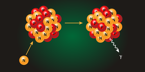
Figure 6 - Artist conception of neutron capture event. (Stonebreaker, 2016)\n",
754 | "\n",
755 | "\n",
756 | "Heavy elements can be formed when neutrons smash into existing elements. The result is a left over proton in the nuclues. Adding a proton to a nucleus means you changed from atom to another. There are 2 types of stellar events that cause the rapid formation of elements: stellar explosions like a supernova and stellar mergers."
757 | ]
758 | },
759 | {
760 | "cell_type": "markdown",
761 | "metadata": {
762 | "id": "2qXGs4-6nPw2"
763 | },
764 | "source": [
765 | "## Neutron Capture r-process & s-process\n",
766 | "In 2017 astronomers observed a neutron star merger or kilonova. This event was so explosive and energetic that scientists observed the gravitational waves from the event. This type of merger is now thought to be the source of many heavy elements. Stellar explosions can cause rapid neutron capture or the r-process.\n",
767 | "\n",
768 | "Sometimes a random neutron inside a star slams into a nucleus and makes a heavier element. This process is rare so it takes a long time to build up an element this way. That's why it's called the slow or s-process.\n",
769 | "\n",
770 | "Europium is thought to mainly come from the r-process, although some europium comes from the s-process.\n",
771 | "
Figure 7 - Neutron capture decay pathway through s-process for xenon. (Sneden et al., 2008)\n"
772 | ]
773 | },
774 | {
775 | "cell_type": "markdown",
776 | "metadata": {
777 | "id": "74TvT2BXgT9R"
778 | },
779 | "source": [
780 | "## Question 7\n",
781 | "**If our target stars have comparable amounts of nickel, what measure should you use based on the results from the code? Rank the stars from most europium detected to least europium detected.**"
782 | ]
783 | },
784 | {
785 | "cell_type": "markdown",
786 | "metadata": {
787 | "id": "sj_0rDoKuXJ-"
788 | },
789 | "source": [
790 | "Double click here to answer:"
791 | ]
792 | },
793 | {
794 | "cell_type": "markdown",
795 | "metadata": {
796 | "id": "e6CPY1W5gzk4"
797 | },
798 | "source": [
799 | "## Question 8\n",
800 | "**These stars all have very similar properties like mass and temperature. Why do they have varying amounts of europium? You should be able to list 3 physical processes by which europium atoms ended up in these stars.**\n"
801 | ]
802 | },
803 | {
804 | "cell_type": "markdown",
805 | "metadata": {
806 | "id": "BDLENLD5uuAf"
807 | },
808 | "source": [
809 | "Double click here to answer:"
810 | ]
811 | },
812 | {
813 | "cell_type": "markdown",
814 | "metadata": {
815 | "id": "yWXV9KAusUd4"
816 | },
817 | "source": [
818 | "# HR Diagram\n",
819 | "Astronomers use the Hertzsprung-Russell Diagram to compare groups of stars and to look for patterns.\n",
820 | "
Figure 8 - H-R diagram for a selected sample of stars. (Fraknoi et al., 2017)\n",
821 | "\n",
822 | "\n",
823 | "Here is a classic example of an HR diagram with some of the known groupings labeled.\n",
824 | "\n",
825 | "If you need a refresher on the HR diagram, take a look [here](https://openstax.org/books/astronomy/pages/18-4-the-h-r-diagram#OSC_Astro_18_04_Sample)"
826 | ]
827 | },
828 | {
829 | "cell_type": "markdown",
830 | "metadata": {
831 | "id": "_UkPn14yuvWb"
832 | },
833 | "source": [
834 | "
Figure 9 - H-R diagram for nearby stars, the sun, and our stellar targets.\n",
835 | "\n",
836 | "\n",
837 | "Here is an HR diagram of some of the nearest stars with our sun and out targets stars also plotted. The main sequence is the grouping of stars running from upper left to lower right and the red giant branch runs from the main sequence off to the upper right."
838 | ]
839 | },
840 | {
841 | "cell_type": "markdown",
842 | "metadata": {
843 | "id": "SUGEtR1DsXsR"
844 | },
845 | "source": [
846 | "## Question 9\n",
847 | "**Using the HR diagram, can you put the results of the EW measurements in context? Are all the targets the same age? What role could the s-process have for these stars?**"
848 | ]
849 | },
850 | {
851 | "cell_type": "markdown",
852 | "metadata": {
853 | "id": "07ldeiM6uz_1"
854 | },
855 | "source": [
856 | "Double click to answer:"
857 | ]
858 | },
859 | {
860 | "cell_type": "markdown",
861 | "metadata": {
862 | "id": "bxnNtsEOwQkJ"
863 | },
864 | "source": [
865 | "# Wrapping up\n",
866 | "\n",
867 | "That's it! Congrats on using code to explore an application of spectroscopy. Feel free to save a copy and explore the code further.\n",
868 | "\n",
869 | "**Be sure and save this completed notebook in your drive and be sure to share it with your instructor!**"
870 | ]
871 | },
872 | {
873 | "cell_type": "markdown",
874 | "metadata": {
875 | "id": "dDKPJ_jnw6qO"
876 | },
877 | "source": [
878 | "## Share and share alike!\n",
879 | "This activity was written by J. Newland and is meant to be shared. If you remix this work, let me know.\n",
880 | "[Reach out for comments or questions.](https://jimmynewland.com)\n",
881 | "\n",
882 | "
This work is licensed under a Creative Commons Attribution-NonCommercial-ShareAlike 4.0 International License.\n",
883 | "\n"
884 | ]
885 | },
886 | {
887 | "cell_type": "markdown",
888 | "metadata": {
889 | "id": "-U0bCa6exLu-"
890 | },
891 | "source": [
892 | "References\n",
893 | "* Commons, W. (2020). File:Nucleosynthesis periodic table.svg --- Wikimedia\n",
894 | "Commons{,} the free media repository. https://commons.wikimedia.org/w/index.php?title=File:Nucleosynthesis_periodic_table.svg&oldid=483860915\n",
895 | "* Fraknoi, A., Morrison, D., Wolff, S. C., OpenStax College, & Rice University. (2017). Astronomy. OpenStax, Rice University. https://openstax.org/details/books/astronomy\n",
896 | "* Newland, J., Grzybowski, E., Hickey, J., Kuper, O., Sneden, C., & Finkelstein, K. (2020). Authentic Astronomical Research as Science Teacher Professional Development.\n",
897 | "https://ui.adsabs.harvard.edu/abs/2020AAS...23536603N/abstract\n",
898 | "* Sakari, C. M., Roederer, I. U., Placco, V. M., Beers, T. C., Ezzeddine, R., Frebel, A., Hansen, T., Sneden, C., Cowan, J. J., Wallerstein, G., Farrell, E. M., Venn, K. A., Matijevič, G., Wyse, R. F. G., Bland-Hawthorn, J., Chiappini, C., Freeman, K. C., Gibson, B. K., Grebel, E. K., … Watson, F. (2019). The R -Process Alliance: Discovery of a Low- α , r -process-enhanced Metal-poor Star in the Galactic Halo . The Astrophysical Journal, 874(2), 148. https://doi.org/10.3847/1538-4357/ab0c02\n",
899 | "* Sneden, C. (2019). Observing Run Research Parameters. UT EXES Teacher Associate Program March 2nd 2019 Conference.\n",
900 | "Sneden, C., Cowan, J. J., & Gallino, R. (2008). Neutron-Capture Elements in the Early Galaxy. Annual Review of Astronomy and Astrophysics, 46(1), 241–288. https://doi.org/10.1146/annurev.astro.46.060407.145207\n",
901 | "* Soubiran, C., Le Campion, J. F., Cayrel De Strobel, G., & Caillo, A. (2010). The PASTEL catalogue of stellar parameters. Astronomy and Astrophysics, 515(11), 1–5. https://doi.org/10.1051/0004-6361/201014264\n",
902 | "* Stonebreaker, A. (2016). Neutron Capture Constraints. Physical Review Letters. https://physics.aps.org/assets/96e56287-2b25-482b-b075-894adc7b2b10/es66_1.png\n"
903 | ]
904 | }
905 | ]
906 | }
--------------------------------------------------------------------------------
/H_R_Diagram_Intro.ipynb:
--------------------------------------------------------------------------------
1 | {
2 | "nbformat": 4,
3 | "nbformat_minor": 0,
4 | "metadata": {
5 | "anaconda-cloud": {},
6 | "kernelspec": {
7 | "display_name": "Python 3",
8 | "language": "python",
9 | "name": "python3"
10 | },
11 | "language_info": {
12 | "codemirror_mode": {
13 | "name": "ipython",
14 | "version": 3
15 | },
16 | "file_extension": ".py",
17 | "mimetype": "text/x-python",
18 | "name": "python",
19 | "nbconvert_exporter": "python",
20 | "pygments_lexer": "ipython3",
21 | "version": "3.7.4"
22 | },
23 | "colab": {
24 | "provenance": [],
25 | "include_colab_link": true
26 | }
27 | },
28 | "cells": [
29 | {
30 | "cell_type": "markdown",
31 | "metadata": {
32 | "id": "view-in-github",
33 | "colab_type": "text"
34 | },
35 | "source": [
36 | ""
37 | ]
38 | },
39 | {
40 | "cell_type": "markdown",
41 | "metadata": {
42 | "id": "3JDakeShaAQH"
43 | },
44 | "source": [
45 | "# Hertzsprung-Russel Diagram Exploration\n",
46 | "This coding activity let's us explore a dataset of stars by plotting something called an H-R Diagram. Astronomers use the Hertzsprung-Russell Diagram to compare groups of stars and to look for patterns.\n",
47 | "\n",
48 | "If you need a refresher on the HR diagram, take a look [here](https://openstax.org/books/astronomy/pages/18-4-the-h-r-diagram#OSC_Astro_18_04_Sample)"
49 | ]
50 | },
51 | {
52 | "cell_type": "markdown",
53 | "metadata": {
54 | "id": "mzRt4wYUXmnr"
55 | },
56 | "source": [
57 | "## Question 1\n",
58 | "**Put your name and period and include anyone working with you as well.**"
59 | ]
60 | },
61 | {
62 | "cell_type": "markdown",
63 | "metadata": {
64 | "id": "lwYsOqYNXwTX"
65 | },
66 | "source": [
67 | "Double click here to answer:"
68 | ]
69 | },
70 | {
71 | "cell_type": "markdown",
72 | "metadata": {
73 | "id": "YIFKsGqT9KNn"
74 | },
75 | "source": [
76 | "# Star catalogue analysis\n",
77 | "This activity analyzes properties of over 100,000 stars.\n",
78 | "\n",
79 | "To get started,\n",
80 | "- You won't hurt anything by experimenting. If you break it, close the tab and open the activity again to start over.\n",
81 | "- Is this your first time? Need a refresher? Try the 5-minute [Intro to Coding activity](https://colab.research.google.com/github/jimmynewland/colabnotebooks/blob/main/Colab_Coding_Intro.ipynb) and come back here.\n",
82 | "\n",
83 | "When you're ready, run each code cell until you get down to **Question 2**."
84 | ]
85 | },
86 | {
87 | "cell_type": "code",
88 | "metadata": {
89 | "id": "6No7X6TC9KNo"
90 | },
91 | "source": [
92 | "# Import modules that contain functions we need\n",
93 | "import pandas as pd\n",
94 | "import numpy as np\n",
95 | "%matplotlib inline\n",
96 | "import matplotlib.pyplot as plt"
97 | ],
98 | "execution_count": null,
99 | "outputs": []
100 | },
101 | {
102 | "cell_type": "code",
103 | "metadata": {
104 | "id": "q3lG6Kle9KNp"
105 | },
106 | "source": [
107 | "# Read in data that will be used for the calculations.\n",
108 | "data = pd.read_csv(\"https://github.com/adamlamee/CODINGinK12/raw/master/data/stars.csv\")"
109 | ],
110 | "execution_count": null,
111 | "outputs": []
112 | },
113 | {
114 | "cell_type": "code",
115 | "metadata": {
116 | "id": "QquuPgqt9KNp"
117 | },
118 | "source": [
119 | "# We wish to look at the first 5 rows of our data set\n",
120 | "data.head(5)"
121 | ],
122 | "execution_count": null,
123 | "outputs": []
124 | },
125 | {
126 | "cell_type": "code",
127 | "metadata": {
128 | "id": "S4gayXWq9KNp"
129 | },
130 | "source": [
131 | "# The .shape command displays the (number of rows , number of columns) in a file.\n",
132 | "data.shape"
133 | ],
134 | "execution_count": null,
135 | "outputs": []
136 | },
137 | {
138 | "cell_type": "markdown",
139 | "metadata": {
140 | "id": "RfzuC0f29KNp"
141 | },
142 | "source": [
143 | "## Question 2\n",
144 | "Let's get acquainted with this data set. Look at the cells above to find the answers to the following questions:\n",
145 | "- In the table above, what do you think each of the column headings represent?\n",
146 | "- How many stars are included in this data set?"
147 | ]
148 | },
149 | {
150 | "cell_type": "markdown",
151 | "metadata": {
152 | "id": "fSIdlLg1YQMt"
153 | },
154 | "source": [
155 | "Double click here to answer:"
156 | ]
157 | },
158 | {
159 | "cell_type": "markdown",
160 | "metadata": {
161 | "id": "OnGodmN8Y8Ax"
162 | },
163 | "source": [
164 | "\n",
165 | "When you're ready, scroll down to **Question 3**."
166 | ]
167 | },
168 | {
169 | "cell_type": "code",
170 | "metadata": {
171 | "id": "h-L2gXo79KNp"
172 | },
173 | "source": [
174 | "fig = plt.figure(figsize=(15, 4))\n",
175 | "plt.scatter(data['ra'],data['dec'], s=0.01)\n",
176 | "plt.xlim(24, 0)\n",
177 | "plt.title(\"What is this?\")\n",
178 | "plt.xlabel(\"x axis?\")\n",
179 | "plt.ylabel(\"y axis\");"
180 | ],
181 | "execution_count": null,
182 | "outputs": []
183 | },
184 | {
185 | "cell_type": "markdown",
186 | "metadata": {
187 | "id": "BapNkLEh9KNp"
188 | },
189 | "source": [
190 | "## Question 3\n",
191 | "The code above generates a plot of **declination** vs. **right ascension** for each star in the data table.\n",
192 | "- The title and axis labels on the plot could use some work. Try editing the code above the plot, then run the code again to see the changes.\n",
193 | "- What pattern do you see in the plot? What might explain that pattern?"
194 | ]
195 | },
196 | {
197 | "cell_type": "markdown",
198 | "metadata": {
199 | "id": "WdiwflmOYZ0k"
200 | },
201 | "source": [
202 | "Double click here to describe patterns in the plot:"
203 | ]
204 | },
205 | {
206 | "cell_type": "markdown",
207 | "metadata": {
208 | "id": "RWUoATC7Y12v"
209 | },
210 | "source": [
211 | "\n",
212 | "When you're ready, scroll down to **Question 4**."
213 | ]
214 | },
215 | {
216 | "cell_type": "code",
217 | "metadata": {
218 | "id": "y4YuzLAc9KNq"
219 | },
220 | "source": [
221 | "# format the points on the plot\n",
222 | "transparency = 0.2\n",
223 | "size = 1\n",
224 | "\n",
225 | "# draws a scatter plot\n",
226 | "plt.scatter(np.log10(data.temp), data.absmag, s=size, edgecolors='none', alpha=transparency)\n",
227 | "plt.xlim(np.log10(15000),np.log10(2000))\n",
228 | "plt.ylim(20,-15)\n",
229 | "plt.title(\"H-R Diagram (log)\")\n",
230 | "plt.ylabel(\"Absolute Magnitude\")\n",
231 | "plt.xlabel(\"Log T (log K)\")"
232 | ],
233 | "execution_count": null,
234 | "outputs": []
235 | },
236 | {
237 | "cell_type": "markdown",
238 | "metadata": {
239 | "id": "sxEtxLTb9KNq"
240 | },
241 | "source": [
242 | "## Question 4\n",
243 | "Use the plot above to answer the following questions:\n",
244 | "- What patterns do you see in the plot?\n",
245 | "- The y-axis shows brighter stars at the top and dimmer stars toward the bottom. What's strange about the **absolute magnitude** scale?\n",
246 | "- Some stars aren't very hot, but they're very bright because they're so big (called *giants* and *super giants*). Where are those on the plot?\n",
247 | "- Other stars are really bright, even though they're small (called *white dwarfs*). How could that happen? Where might you find them on the plot?"
248 | ]
249 | },
250 | {
251 | "cell_type": "markdown",
252 | "metadata": {
253 | "id": "NojOQKCLZmrx"
254 | },
255 | "source": [
256 | "Double click to answer:"
257 | ]
258 | },
259 | {
260 | "cell_type": "markdown",
261 | "metadata": {
262 | "id": "vwG5dveoZl4U"
263 | },
264 | "source": [
265 | "When you're ready, scroll down to **Question 5**."
266 | ]
267 | },
268 | {
269 | "cell_type": "code",
270 | "metadata": {
271 | "id": "eRrmnEsR9KNq"
272 | },
273 | "source": [
274 | "# These are the abbreviations for all the constellations\n",
275 | "data['con'].sort_values().unique()"
276 | ],
277 | "execution_count": null,
278 | "outputs": []
279 | },
280 | {
281 | "cell_type": "code",
282 | "metadata": {
283 | "id": "HQs7xGuK9KNq"
284 | },
285 | "source": [
286 | "# This picks a constellation to plot\n",
287 | "constellation = data.query('con == \"Ori\"') # Ori is short for Orion\n",
288 | "\n",
289 | "plt.close('all')\n",
290 | "fig = plt.figure(figsize=(12, 5))\n",
291 | "plt.subplot(1, 2, 1)\n",
292 | "\n",
293 | "# This plots where the constellation's 10 brightest stars are in the sky\n",
294 | "constellation = constellation.sort_values('mag').head(10)\n",
295 | "plt.scatter(constellation['ra'],constellation['dec'])\n",
296 | "plt.gca().invert_xaxis()\n",
297 | "plt.title(\"A constellation in the sky\")\n",
298 | "plt.xlabel(\"right ascension\")\n",
299 | "plt.ylabel(\"declination\")\n",
300 | "\n",
301 | "plt.subplot(1, 2, 2)\n",
302 | "# format the points on the plot\n",
303 | "transparency = 0.2\n",
304 | "size = 1\n",
305 | "\n",
306 | "# plots the constellation's stars in red over the big plot of all stars\n",
307 | "plt.scatter(np.log10(data['temp']), data['absmag'], s=size, edgecolors='none', alpha=transparency)\n",
308 | "logtemps = np.log10(constellation['temp'])\n",
309 | "#plt.scatter(constellation['temp'], constellation['absmag'], color='red', edgecolors='none')\n",
310 | "plt.scatter(logtemps, constellation['absmag'], color='red', edgecolors='none')\n",
311 | "#plt.xlim(2000,15000)\n",
312 | "plt.xlim(np.log10(15000),np.log10(2000))\n",
313 | "plt.ylim(20,-15)\n",
314 | "plt.title(\"Types of stars in a constellation\")\n",
315 | "plt.ylabel(\"Absolute Magnitude\")\n",
316 | "plt.xlabel(\"log Temp (logK)\")\n",
317 | "plt.show()"
318 | ],
319 | "execution_count": null,
320 | "outputs": []
321 | },
322 | {
323 | "cell_type": "markdown",
324 | "metadata": {
325 | "id": "ivfXlh_k9KNq"
326 | },
327 | "source": [
328 | "## Question Five\n",
329 | "The left plot above shows what the constellation **Orion** looks like in the sky. The plot on the right shows those same stars (as red points) on the same absolute magnitude vs. temperature plot in part two.\n",
330 | "- Using the graphic below, which types of stars are in Orion?\n",
331 | "- The code above shows the abbreviation for each constellation, then lets you filter the data set for just the stars in that constellation (called a *query*). Try plotting a different constellation, like Cassiopeia. Is it made of different types of stars?\n",
332 | "
Figure 1 - H-R diagram for a selected sample of stars. (Fraknoi et al., 2017)\n",
333 | "\n"
334 | ]
335 | },
336 | {
337 | "cell_type": "markdown",
338 | "source": [],
339 | "metadata": {
340 | "id": "90gaVrIQ_8lw"
341 | }
342 | },
343 | {
344 | "cell_type": "markdown",
345 | "source": [
346 | "---\n",
347 | "## Saving Your Work\n",
348 | "This is running on a Google server on a distant planet and deletes what you've done when you close this tab. To save your work for later use or analysis you have a few options:\n",
349 | "- File > \"Save a copy in Drive\" will save it to you Google Drive in a folder called \"Collaboratory\". You can run it later from there.\n",
350 | "- File > \"Download .ipynb\" to save to your computer (and run with Jupyter software later)\n",
351 | "- File > Print to ... um ... print.\n",
352 | "- To save an image of a plot or chart, right-click on it and select Save Image as ...\n",
353 | "\n",
354 | "## Credits\n",
355 | "The data came from [The Astronomy Nexus](http://www.astronexus.com/hyg) and their collection of the Hipparcos, Yale Bright Star, and Gliese catalogues ([huge zip file here](http://www.astronexus.com/files/downloads/hygdata_v3.csv.gz)).\n",
356 | "\n",
357 | "UCF physics undergraduate Tyler Townsend, who located the data and began the analysis, was funded by Seminole County Schools to make scientific computing a standard part of every middle school science class. The Mily Way scatterplot was added by [Quarknet](https://quarknet.i2u2.org/) Fellow and high school teacher Jeremy Smith, Baltimore, MD. This notebook was designed by [Adam LaMee](https://adamlamee.github.io/), who coordinated its development as the [PhysTEC](https://www.phystec.org/) Teacher-in-residence in the [University of Central Florida's Physics department](https://sciences.ucf.edu/physics/). Find more of Adam LaMee's activities at [CODINGinK12.org](http://www.codingink12.org)."
358 | ],
359 | "metadata": {
360 | "id": "MqRsjjID_1z3"
361 | }
362 | }
363 | ]
364 | }
--------------------------------------------------------------------------------
/Keplers_3rd_Law_Activity.ipynb:
--------------------------------------------------------------------------------
1 | {
2 | "nbformat": 4,
3 | "nbformat_minor": 0,
4 | "metadata": {
5 | "anaconda-cloud": {},
6 | "kernelspec": {
7 | "display_name": "Python 3",
8 | "language": "python",
9 | "name": "python3"
10 | },
11 | "language_info": {
12 | "codemirror_mode": {
13 | "name": "ipython",
14 | "version": 3
15 | },
16 | "file_extension": ".py",
17 | "mimetype": "text/x-python",
18 | "name": "python",
19 | "nbconvert_exporter": "python",
20 | "pygments_lexer": "ipython3",
21 | "version": "3.7.4"
22 | },
23 | "colab": {
24 | "name": "Keplers 3rd Law Activity.ipynb",
25 | "provenance": [],
26 | "include_colab_link": true
27 | }
28 | },
29 | "cells": [
30 | {
31 | "cell_type": "markdown",
32 | "metadata": {
33 | "id": "view-in-github",
34 | "colab_type": "text"
35 | },
36 | "source": [
37 | ""
38 | ]
39 | },
40 | {
41 | "cell_type": "markdown",
42 | "metadata": {
43 | "id": "3JDakeShaAQH"
44 | },
45 | "source": [
46 | "# Kepler's 3rd Law Activity Using Data\n",
47 | "This coding activity let's us explore some data gathered by the [Kepler spacecraft](https://archive.stsci.edu/missions-and-data/kepler) of a single set of planets orbiting a star a lot like the sun.\n",
48 | "\n",
49 | " \n",
50 | "\n",
51 | "The Kepler Spacecraft has help uncovered many exoplanets. When a planet passes in front of the host star, the Kepler photometer and camera measure the tiny drop in light. We are going to explore one of these planetary systems. With the data about an exoplanetary system, you must determine the approximate mass of the central star of the system. The units given are in terms of astronomical units and days. You should report the mass of the star in solar mass units. In other words what factor of the sun's mass is this star?\n",
52 | "\n",
53 | "
\n",
50 | "\n",
51 | "The Kepler Spacecraft has help uncovered many exoplanets. When a planet passes in front of the host star, the Kepler photometer and camera measure the tiny drop in light. We are going to explore one of these planetary systems. With the data about an exoplanetary system, you must determine the approximate mass of the central star of the system. The units given are in terms of astronomical units and days. You should report the mass of the star in solar mass units. In other words what factor of the sun's mass is this star?\n",
52 | "\n",
53 | " \n",
54 | "\n",
55 | "\n",
56 | "The planetary data (period, T, in days and average distance from the star, a, in AU) is given in the table linked below. The period, T, is given in Earth days (not Earth years!) and the semi-major axis, a, is given in astronomical units. Using Kepler’s 3rd law of planetary motion, linearize the data with appropriate units to determine the mass of the central star of the given system as a ratio of solar mass.\n",
57 | "\n"
58 | ]
59 | },
60 | {
61 | "cell_type": "markdown",
62 | "metadata": {
63 | "id": "mzRt4wYUXmnr"
64 | },
65 | "source": [
66 | "## Question 1\n",
67 | "**Put your name and period and include anyone working with you as well.**"
68 | ]
69 | },
70 | {
71 | "cell_type": "markdown",
72 | "metadata": {
73 | "id": "lwYsOqYNXwTX"
74 | },
75 | "source": [
76 | "Double click here to answer:"
77 | ]
78 | },
79 | {
80 | "cell_type": "markdown",
81 | "metadata": {
82 | "id": "kq_1DmVTb8ft"
83 | },
84 | "source": [
85 | "**Don't forget to run each block as you scroll!**"
86 | ]
87 | },
88 | {
89 | "cell_type": "code",
90 | "metadata": {
91 | "id": "6No7X6TC9KNo"
92 | },
93 | "source": [
94 | "# Import modules that contain functions we need\n",
95 | "import pandas as pd # pandas is common for data science\n",
96 | "import numpy as np #N umPy is used a lot in science\n",
97 | "import math # we need the math class for pi\n",
98 | "%matplotlib inline\n",
99 | "import matplotlib.pyplot as plt # MatPlotLib is the plotting standard\n",
100 | "import seaborn as sns # makes regression plot easy\n",
101 | "from scipy import stats # lets us do a linear regression"
102 | ],
103 | "execution_count": null,
104 | "outputs": []
105 | },
106 | {
107 | "cell_type": "markdown",
108 | "metadata": {
109 | "id": "z72DEuJGVg7F"
110 | },
111 | "source": [
112 | "## Constants\n",
113 | "The distance from the Earth to the Sun is known as an astromical unit but we will need to convert those distances to meters. The constant, G, is the universal gravitational constant. We will also need the mass of the sun in kilograms to round out our dependence on SI units.\n",
114 | "$$\n",
115 | "d_{au}=1.5\\times10^{11} \\mathrm{m} \\\\\n",
116 | "G=6.67\\times10^{-11} \\mathrm{Nm^2/kg^2} \\\\\n",
117 | "M_{sun}=1.989\\times10^{30} \\mathrm{kg}\n",
118 | "$$\n"
119 | ]
120 | },
121 | {
122 | "cell_type": "code",
123 | "metadata": {
124 | "id": "xUfovvQpLYJN"
125 | },
126 | "source": [
127 | "# Type the constants here in standard units.\n",
128 | "# Example: 3*10^8 in Python would be 3e8\n",
129 | "d_au = 1 # put the correct value in meters here\n",
130 | "G = 1 # put the correct value in Nm^2/kg^2\n",
131 | "m_sun = 1 # put the correct value in kg"
132 | ],
133 | "execution_count": null,
134 | "outputs": []
135 | },
136 | {
137 | "cell_type": "markdown",
138 | "metadata": {
139 | "id": "cwT7EtBIX6P8"
140 | },
141 | "source": [
142 | "# Kepler Exoplanet Data\n",
143 | "This dataset is based on the discovery of an exolplanet system by the Kepler Spacecraft, named after Johannes Kepler, who, in the seventeenth century, determined the planetary motion relationships using data collected by Tycho."
144 | ]
145 | },
146 | {
147 | "cell_type": "code",
148 | "metadata": {
149 | "id": "q3lG6Kle9KNp"
150 | },
151 | "source": [
152 | "# Read in data that will be used for the calculations.\n",
153 | "df = pd.read_csv(\"https://thinkingwithcode.com/datascience/kepler-planetary-data.csv\")"
154 | ],
155 | "execution_count": null,
156 | "outputs": []
157 | },
158 | {
159 | "cell_type": "markdown",
160 | "metadata": {
161 | "id": "qtILmt8NZVbV"
162 | },
163 | "source": [
164 | "# Column Headings\n",
165 | "We need to use the
\n",
54 | "\n",
55 | "\n",
56 | "The planetary data (period, T, in days and average distance from the star, a, in AU) is given in the table linked below. The period, T, is given in Earth days (not Earth years!) and the semi-major axis, a, is given in astronomical units. Using Kepler’s 3rd law of planetary motion, linearize the data with appropriate units to determine the mass of the central star of the given system as a ratio of solar mass.\n",
57 | "\n"
58 | ]
59 | },
60 | {
61 | "cell_type": "markdown",
62 | "metadata": {
63 | "id": "mzRt4wYUXmnr"
64 | },
65 | "source": [
66 | "## Question 1\n",
67 | "**Put your name and period and include anyone working with you as well.**"
68 | ]
69 | },
70 | {
71 | "cell_type": "markdown",
72 | "metadata": {
73 | "id": "lwYsOqYNXwTX"
74 | },
75 | "source": [
76 | "Double click here to answer:"
77 | ]
78 | },
79 | {
80 | "cell_type": "markdown",
81 | "metadata": {
82 | "id": "kq_1DmVTb8ft"
83 | },
84 | "source": [
85 | "**Don't forget to run each block as you scroll!**"
86 | ]
87 | },
88 | {
89 | "cell_type": "code",
90 | "metadata": {
91 | "id": "6No7X6TC9KNo"
92 | },
93 | "source": [
94 | "# Import modules that contain functions we need\n",
95 | "import pandas as pd # pandas is common for data science\n",
96 | "import numpy as np #N umPy is used a lot in science\n",
97 | "import math # we need the math class for pi\n",
98 | "%matplotlib inline\n",
99 | "import matplotlib.pyplot as plt # MatPlotLib is the plotting standard\n",
100 | "import seaborn as sns # makes regression plot easy\n",
101 | "from scipy import stats # lets us do a linear regression"
102 | ],
103 | "execution_count": null,
104 | "outputs": []
105 | },
106 | {
107 | "cell_type": "markdown",
108 | "metadata": {
109 | "id": "z72DEuJGVg7F"
110 | },
111 | "source": [
112 | "## Constants\n",
113 | "The distance from the Earth to the Sun is known as an astromical unit but we will need to convert those distances to meters. The constant, G, is the universal gravitational constant. We will also need the mass of the sun in kilograms to round out our dependence on SI units.\n",
114 | "$$\n",
115 | "d_{au}=1.5\\times10^{11} \\mathrm{m} \\\\\n",
116 | "G=6.67\\times10^{-11} \\mathrm{Nm^2/kg^2} \\\\\n",
117 | "M_{sun}=1.989\\times10^{30} \\mathrm{kg}\n",
118 | "$$\n"
119 | ]
120 | },
121 | {
122 | "cell_type": "code",
123 | "metadata": {
124 | "id": "xUfovvQpLYJN"
125 | },
126 | "source": [
127 | "# Type the constants here in standard units.\n",
128 | "# Example: 3*10^8 in Python would be 3e8\n",
129 | "d_au = 1 # put the correct value in meters here\n",
130 | "G = 1 # put the correct value in Nm^2/kg^2\n",
131 | "m_sun = 1 # put the correct value in kg"
132 | ],
133 | "execution_count": null,
134 | "outputs": []
135 | },
136 | {
137 | "cell_type": "markdown",
138 | "metadata": {
139 | "id": "cwT7EtBIX6P8"
140 | },
141 | "source": [
142 | "# Kepler Exoplanet Data\n",
143 | "This dataset is based on the discovery of an exolplanet system by the Kepler Spacecraft, named after Johannes Kepler, who, in the seventeenth century, determined the planetary motion relationships using data collected by Tycho."
144 | ]
145 | },
146 | {
147 | "cell_type": "code",
148 | "metadata": {
149 | "id": "q3lG6Kle9KNp"
150 | },
151 | "source": [
152 | "# Read in data that will be used for the calculations.\n",
153 | "df = pd.read_csv(\"https://thinkingwithcode.com/datascience/kepler-planetary-data.csv\")"
154 | ],
155 | "execution_count": null,
156 | "outputs": []
157 | },
158 | {
159 | "cell_type": "markdown",
160 | "metadata": {
161 | "id": "qtILmt8NZVbV"
162 | },
163 | "source": [
164 | "# Column Headings\n",
165 | "We need to use the head() command to take a peek at the data but also to know the names of the column headings so we access the data. When we load a datafile using pandas, the data is stored in a thing called a DataFrame. Here data1 is a DataFrame."
166 | ]
167 | },
168 | {
169 | "cell_type": "code",
170 | "metadata": {
171 | "id": "QquuPgqt9KNp"
172 | },
173 | "source": [
174 | "# We wish to look at the first 5 rows of our data set\n",
175 | "df.head(5)"
176 | ],
177 | "execution_count": null,
178 | "outputs": []
179 | },
180 | {
181 | "cell_type": "markdown",
182 | "metadata": {
183 | "id": "i0clFzF7H2xs"
184 | },
185 | "source": [
186 | "A DataFrame is kind of like a spreadsheet. There are rows and columns of data so it is a 2d data structure."
187 | ]
188 | },
189 | {
190 | "cell_type": "code",
191 | "metadata": {
192 | "id": "S4gayXWq9KNp"
193 | },
194 | "source": [
195 | "# The .shape command displays the (number of rows , number of columns) in a file.\n",
196 | "df.shape"
197 | ],
198 | "execution_count": null,
199 | "outputs": []
200 | },
201 | {
202 | "cell_type": "markdown",
203 | "metadata": {
204 | "id": "RfzuC0f29KNp"
205 | },
206 | "source": [
207 | "## Question 2\n",
208 | "Let's get acquainted with this data set. Look at the cells above to find the answers to the following questions:\n",
209 | "- In the table above, what do you think each of the column headings represent?\n",
210 | "- How many planets are included in this data set?"
211 | ]
212 | },
213 | {
214 | "cell_type": "markdown",
215 | "metadata": {
216 | "id": "fSIdlLg1YQMt"
217 | },
218 | "source": [
219 | "Double click here to answer:"
220 | ]
221 | },
222 | {
223 | "cell_type": "markdown",
224 | "metadata": {
225 | "id": "OnGodmN8Y8Ax"
226 | },
227 | "source": [
228 | "\n",
229 | "These lines store all the distances in AU in a list called r_au and all the periods in a list called t_days. Don't forget to run this block like the other blocks before this."
230 | ]
231 | },
232 | {
233 | "cell_type": "code",
234 | "metadata": {
235 | "id": "1_gTK9FxK_WN"
236 | },
237 | "source": [
238 | "r_au = np.array(df['Semi Major Axis (AU)']) # extract the distance data from df\n",
239 | "t_days = np.array(df['Orbital Period (days)']) # extract the time data from df"
240 | ],
241 | "execution_count": null,
242 | "outputs": []
243 | },
244 | {
245 | "cell_type": "markdown",
246 | "metadata": {
247 | "id": "htdjMoxZaxOV"
248 | },
249 | "source": [
250 | "This is a very stripped down plot using MatPlotLib. You need to fix the title and the labels on the x- and y-axes."
251 | ]
252 | },
253 | {
254 | "cell_type": "code",
255 | "metadata": {
256 | "id": "h-L2gXo79KNp"
257 | },
258 | "source": [
259 | "# plt is our plot object which handles plotting data\n",
260 | "# For physics and astronomy, you probably want a scatter plot\n",
261 | "\n",
262 | "# plt.scatter uses the 1st thing for the horizontal axis\n",
263 | "# and the 2nd thing for the vertical axis so (x,y)\n",
264 | "plt.scatter(r_au, t_days)\n",
265 | "plt.title(\"title?\")\n",
266 | "plt.xlabel(\"Label me!\")\n",
267 | "plt.ylabel(\"Me, too!\");"
268 | ],
269 | "execution_count": null,
270 | "outputs": []
271 | },
272 | {
273 | "cell_type": "markdown",
274 | "metadata": {
275 | "id": "U7LaBcMw5v0K"
276 | },
277 | "source": [
278 | "# Convert Distances and Times\n",
279 | "Convert the orbital radii from AU to meters using the constant above. Also convert the times from days into seconds. This is straightforward dimensional analysis."
280 | ]
281 | },
282 | {
283 | "cell_type": "code",
284 | "metadata": {
285 | "id": "piMmulxkL1K4"
286 | },
287 | "source": [
288 | "# Convert AU to m using one of the constants above\n",
289 | "r_m = r_au * 1 # use the correct constant instead of 1\n",
290 | "\n",
291 | "# How many seconds are in a day? Use that to change t_days\n",
292 | "t_s = t_days * 1 # use the correct constant instead of 1"
293 | ],
294 | "execution_count": null,
295 | "outputs": []
296 | },
297 | {
298 | "cell_type": "markdown",
299 | "metadata": {
300 | "id": "sVC5h1la5vfM"
301 | },
302 | "source": [
303 | "# Linearize the Data\n",
304 | "Using Kepler's 3rd law, linearize your data. Kepler's 3rd law:\n",
305 | "$$ t^2=\\frac{4\\pi^2}{GM}r^3 $$"
306 | ]
307 | },
308 | {
309 | "cell_type": "markdown",
310 | "metadata": {
311 | "id": "y3FV1CsFbUmB"
312 | },
313 | "source": [
314 | "Store the linearized distances in the list called x and the linearized times in the list called y.\n",
315 | "\n",
316 | "**This part is important! The data won't be linear if you don't apply the correct mathematical process to your various lists of data.**"
317 | ]
318 | },
319 | {
320 | "cell_type": "code",
321 | "metadata": {
322 | "id": "0kuccApsNVMC"
323 | },
324 | "source": [
325 | "# Hint: In Python, exponents work like this\n",
326 | "# a^2 (a squared) would be a**2\n",
327 | "x = r_m # Change for x-axis based on equation above? (Hint: use distance somehow)\n",
328 | "y = t_s # Change for y-axis based on equation above? (Hint: use time somehow)"
329 | ],
330 | "execution_count": null,
331 | "outputs": []
332 | },
333 | {
334 | "cell_type": "code",
335 | "metadata": {
336 | "id": "vMunIR5XNkQx"
337 | },
338 | "source": [
339 | "plt.scatter(x,y)\n",
340 | "plt.title(\"title?\")\n",
341 | "plt.xlabel(\"Label me!\")\n",
342 | "plt.ylabel(\"Me, too!\");"
343 | ],
344 | "execution_count": null,
345 | "outputs": []
346 | },
347 | {
348 | "cell_type": "markdown",
349 | "metadata": {
350 | "id": "stW4WSuYcSTe"
351 | },
352 | "source": [
353 | "# Linear Regression\n",
354 | "This line of code uses our data in the lists x and y to find the various parameters for a linear regression. We ultimately only will need the slope here. Remember, a linear regression is asking how close to linear is the mathematical relationship between our x and y variables.\n",
355 | "\n",
356 | "For someone new to this python notation, the command (or method or function) called linregress(...) takes as one input our list of linearized distances as the list x and takes as the other input our list of linearized times as the list y. But it is all the stuff on the left of the = that's likely weird to you. The linregress command returns 5 things by default: the slope of our linear fit, the intercept of our linear fit, and some statistics about the quality of the fit. The *r*, *p*, and *standard error* values help us decide of the fit is trustworthy in a statical sense. We will ignore them here."
357 | ]
358 | },
359 | {
360 | "cell_type": "code",
361 | "metadata": {
362 | "id": "gv4eOvWVPVZf"
363 | },
364 | "source": [
365 | "# get coefficients of our linear fit\n",
366 | "slope, intercept, r_value, p_value, std_err = stats.linregress(x,y)"
367 | ],
368 | "execution_count": null,
369 | "outputs": []
370 | },
371 | {
372 | "cell_type": "markdown",
373 | "metadata": {
374 | "id": "vhipzmtHcfH3"
375 | },
376 | "source": [
377 | "# Make a New DataFrame\n",
378 | "By putting the linearized data in a new DataFrame, we can easily plot a linear regression using Seaborn. This is a common data science technique."
379 | ]
380 | },
381 | {
382 | "cell_type": "code",
383 | "metadata": {
384 | "id": "yQGwuHaozWUs"
385 | },
386 | "source": [
387 | "# Make a new DataFrame and take a look at it.\n",
388 | "df2 = pd.DataFrame({'r^3 (m^3)':x, 't^2 (s^2)':y})\n",
389 | "\n",
390 | "# Append the new data to the original dataframe\n",
391 | "df = pd.concat([df, df2], axis=1)\n",
392 | "\n",
393 | "df.head()"
394 | ],
395 | "execution_count": null,
396 | "outputs": []
397 | },
398 | {
399 | "cell_type": "markdown",
400 | "metadata": {
401 | "id": "I88m3YWXJuiO"
402 | },
403 | "source": [
404 | "If you've done the rest of this process correctly, here you need to recognize which parts of Kepler's 3rd Law is the *slope* of our linear relationship. The slope of a line should a constant so which parts are constant here?\n",
405 | "$$ t^2=\\frac{4\\pi^2}{GM}r^3 $$\n",
406 | "\n",
407 | "Using the slope from the regression above, if you set the slope equal to the constants from Kepler's 3rd Law, rearrange algebraically (on paper likely) the expression such that you can find the mass of the star in the center of this exoplanet solar system.\n"
408 | ]
409 | },
410 | {
411 | "cell_type": "code",
412 | "metadata": {
413 | "id": "A3SfsnYJwlJl"
414 | },
415 | "source": [
416 | "# Use the algebraically rearranged slope expression\n",
417 | "# to find the mass of the star in this system.\n",
418 | "m_star = (1 * 1)/(1 * 1) # replace right hand side using correct algebra & constants\n",
419 | "\n",
420 | "# Find the ratio of this star's mass to that of the sun, given above.\n",
421 | "ratio = m_star / 1 # replace 1 with correct constant\n",
422 | "\n",
423 | "# Display the ratio.\n",
424 | "print(ratio)"
425 | ],
426 | "execution_count": null,
427 | "outputs": []
428 | },
429 | {
430 | "cell_type": "markdown",
431 | "metadata": {
432 | "id": "qUAGvQ7XLV6p"
433 | },
434 | "source": [
435 | "# Plot Linear Regression\n",
436 | "This last step uses the Seaborn library to plot linear regression and to overplot the data points. This is a very common visualization technique and allows for a visual confirmation of the relationship. Seaborn is not the only way to plot a linear regression but it is very popular and quite visually appealing."
437 | ]
438 | },
439 | {
440 | "cell_type": "code",
441 | "metadata": {
442 | "id": "TS8L4GbdwvdV"
443 | },
444 | "source": [
445 | "sns.regplot(x=\"r^3 (m^3)\", y=\"t^2 (s^2)\", data=df2)"
446 | ],
447 | "execution_count": null,
448 | "outputs": []
449 | },
450 | {
451 | "cell_type": "markdown",
452 | "source": [
453 | "Kepler's Third Law Activity © 2025 by Dr. James Newland is licensed under CC BY-NC-SA 4.0 "
454 | ],
455 | "metadata": {
456 | "id": "RhKiaMp0ZLvw"
457 | }
458 | }
459 | ]
460 | }
--------------------------------------------------------------------------------
/NGC_3201_Photometry_Student.ipynb:
--------------------------------------------------------------------------------
1 | {
2 | "nbformat": 4,
3 | "nbformat_minor": 0,
4 | "metadata": {
5 | "kernelspec": {
6 | "display_name": "Python 3",
7 | "language": "python",
8 | "name": "python3"
9 | },
10 | "language_info": {
11 | "codemirror_mode": {
12 | "name": "ipython",
13 | "version": 3
14 | },
15 | "file_extension": ".py",
16 | "mimetype": "text/x-python",
17 | "name": "python",
18 | "nbconvert_exporter": "python",
19 | "pygments_lexer": "ipython3",
20 | "version": "3.6.8"
21 | },
22 | "colab": {
23 | "name": "NGC 3201 Photometry_Student.ipynb",
24 | "provenance": [],
25 | "include_colab_link": true
26 | }
27 | },
28 | "cells": [
29 | {
30 | "cell_type": "markdown",
31 | "metadata": {
32 | "id": "view-in-github",
33 | "colab_type": "text"
34 | },
35 | "source": [
36 | ""
37 | ]
38 | },
39 | {
40 | "cell_type": "markdown",
41 | "metadata": {
42 | "id": "Sfy3RMEsm9UL"
43 | },
44 | "source": [
45 | "# Measuring distance with light\n",
46 | "## RR Lyrae Stars as Standard Candles"
47 | ]
48 | },
49 | {
50 | "cell_type": "markdown",
51 | "metadata": {
52 | "id": "w8FfOBmJm9UN"
53 | },
54 | "source": [
55 | "How can we measure astronomical distances? One technique is to use \"standard candles\", which are astronomical objects that have well-known brightnesses. By measuring how bright an object appears to us and knowing the actual brightness from some analysis, we can work out how far the object is from us. We employ the \"inverse square law\" for light to make this happen and do a bit of math.\n",
56 | "\n",
57 | "
"
454 | ],
455 | "metadata": {
456 | "id": "RhKiaMp0ZLvw"
457 | }
458 | }
459 | ]
460 | }
--------------------------------------------------------------------------------
/NGC_3201_Photometry_Student.ipynb:
--------------------------------------------------------------------------------
1 | {
2 | "nbformat": 4,
3 | "nbformat_minor": 0,
4 | "metadata": {
5 | "kernelspec": {
6 | "display_name": "Python 3",
7 | "language": "python",
8 | "name": "python3"
9 | },
10 | "language_info": {
11 | "codemirror_mode": {
12 | "name": "ipython",
13 | "version": 3
14 | },
15 | "file_extension": ".py",
16 | "mimetype": "text/x-python",
17 | "name": "python",
18 | "nbconvert_exporter": "python",
19 | "pygments_lexer": "ipython3",
20 | "version": "3.6.8"
21 | },
22 | "colab": {
23 | "name": "NGC 3201 Photometry_Student.ipynb",
24 | "provenance": [],
25 | "include_colab_link": true
26 | }
27 | },
28 | "cells": [
29 | {
30 | "cell_type": "markdown",
31 | "metadata": {
32 | "id": "view-in-github",
33 | "colab_type": "text"
34 | },
35 | "source": [
36 | ""
37 | ]
38 | },
39 | {
40 | "cell_type": "markdown",
41 | "metadata": {
42 | "id": "Sfy3RMEsm9UL"
43 | },
44 | "source": [
45 | "# Measuring distance with light\n",
46 | "## RR Lyrae Stars as Standard Candles"
47 | ]
48 | },
49 | {
50 | "cell_type": "markdown",
51 | "metadata": {
52 | "id": "w8FfOBmJm9UN"
53 | },
54 | "source": [
55 | "How can we measure astronomical distances? One technique is to use \"standard candles\", which are astronomical objects that have well-known brightnesses. By measuring how bright an object appears to us and knowing the actual brightness from some analysis, we can work out how far the object is from us. We employ the \"inverse square law\" for light to make this happen and do a bit of math.\n",
56 | "\n",
57 | " Look for the variable stars. They seem to blink.
\n",
58 | "\n",
59 | "## Need more on how we use variable stars to measure distance?\n",
60 | "If you are new to the idea of variable stars as tools for measuring distances, start with these:\n",
61 | "* [OpenStax Astronomy: Variable Stars - One Key to Cosmic Distances](https://cnx.org/contents/LnN76Opl@21.8:vdWWIntw@8/19-3-Variable-Stars-One-Key-to-Cosmic-Distances). \n",
62 | "* [Measuring the the Milky Way with RR Lyrae Stars, a presentation by J Newland](https://docs.google.com/presentation/d/18IaOORqe0qh4A5u7A5SULAgiyDVl1sOz0sP0g7rmOns/edit?usp=sharing) "
63 | ]
64 | },
65 | {
66 | "cell_type": "markdown",
67 | "metadata": {
68 | "id": "ccNGJpHKm9UO"
69 | },
70 | "source": [
71 | "## Inverse Square Law\n",
72 | "When light leaves the surface of an astronomical object, like a star's photosphere, the resulting light spreads out radially in all directions at the speed of light. All the energy emitted at that same instant can be thought of as being spread out over surface of a sphere. As this imaginary sphere gets bigger, the light gets more spread out. This is why distance matters when looking at a light source. Note the equation for the surface area of a sphere:\n",
73 | "\\begin{equation*}\n",
74 | "A=4\\pi{R^2}\n",
75 | "\\end{equation*}\n",
76 | "The closer you are, the more concentrated the light is because the sphere over which it is spread is smaller (smaller radius, R). The farther you get from the source, the bigger the sphere must be when it reaches you (larger radius, R) and consequently, the light is spread out more and so the source seems dimmer.\n",
77 | "
Illustration of inverse square law.
\n",
78 | "\n",
79 | "The physical properties of electromagnetic radiation eminating from a star or other astronomical object is best described using flux which is related to power which is related to energy. Another common way to describe light leaving an astronomical object is through the concept of luminosity. The Stefan-Boltzman relation connections the energy density of a star (how much energy leaves 1 square meter of the star's surfce) and the star's temperature.\n",
80 | "\n",
81 | "\\begin{equation*}\n",
82 | "L=\\sigma{T^4}\\>[\\mathbf{W/m^2}]\n",
83 | "\\end{equation*}\n",
84 | "\n",
85 | "We can find the power emitted by the star if we include the entire spherical surface of the star\n",
86 | "\n",
87 | "\\begin{equation*}\n",
88 | "L=\\sigma{T^4}(4\\pi{R^2})\\>[\\mathbf{W}]\n",
89 | "\\end{equation*}\n",
90 | "\n",
91 | "Don't forget that astronomers can determine the surface temperature of a star using Wien's law. Once the peak wavelength of the light from the star is found, we can get the temperature using the relation:\n",
92 | "\n",
93 | "\\begin{equation*}\n",
94 | "\\lambda_{peak}\\cdot{T}=constant\\>[\\mathbf{m\\cdot{K}}]\n",
95 | "\\end{equation*}\n",
96 | "\n",
97 | "## Magnitude vs Luminosity\n",
98 | "For historical and convenience reasons, astronomers use a system called magnitude dating back to Hipparcos which uses the star Vega as a reference star. There are many peculiarlities with magnitude. For example a negative magnitude represents a brighter object than does a positive magnitude. Another useful point is that just using light from an image, astronomers can quickly measure the magnitude as seen from earth, the apparent magnitude. That leaves some work to do to get turn the physical brightness or luminosity of the object into the absolute magnitude. The magnitude scale is clunky but still in use - for now."
99 | ]
100 | },
101 | {
102 | "cell_type": "markdown",
103 | "metadata": {
104 | "id": "Xv71YBjOm9UO"
105 | },
106 | "source": [
107 | "## Globular Clusters\n",
108 | "A globular cluster is a very old grouping of stars usually found in the halo or the central region of a galaxy. NGC 3201 is one such globular cluster found in the Milky Way Galaxy. The images used for this activity were taken using the [Skynet Robitic Telescope Network](https://skynet.unc.edu/) run by the University of North Carolina. Yes... they called a robotic telescope system Skynet. The globular cluster was imaged 5 times in a single night by the system. This way, any star that has a periodic change of a day or so will show up in the series of images.\n",
109 | "\n",
110 | "\n",
111 | " \n",
112 | "Globular Cluster NGC 3201
\n",
112 | "Globular Cluster NGC 3201
\n",
113 | "\n",
114 | "For this activity, we are going to study images taken of a variable star in a globular cluster over a single night. This star is known as an RR Lyrae variable star which varies over a period of less than one day. All stars that fall into this class have approximately the same absolute luminosity. That means if all RR Lyrae stars were the same distance from the observer, they would all appear the same brightness.\n",
115 | "\n",
116 | "But stars are, of course, spread out across a galaxy and ours is no exception. So RR Lyrae stars appear to be different brightnesses due to their distances. "
117 | ]
118 | },
119 | {
120 | "cell_type": "markdown",
121 | "metadata": {
122 | "id": "qKB0ILNPm9UP"
123 | },
124 | "source": [
125 | "## Choosing a target\n",
126 | "We will study [one such star](http://simbad.u-strasbg.fr/simbad/sim-id?Ident=Cl*+NGC+3201+++++LS+++++358&NbIdent=1) in a globular cluster visible from Earth's southern hemisphere.\n",
127 | "\n",
128 | "In order to determine the magnitude of the star, we will need a [known calibration star](http://simbad.u-strasbg.fr/simbad/sim-id?Ident=Cl*+NGC+3201+++CWFD++3-106&NbIdent=1) that is in the field and near the target star. Note that here we have zoomed in a lot on our target star. At this level in this image the only things visible are stars (no galaxies or such) and almost every star visible is a part of the globular cluster.\n",
129 | "\n",
130 | " Zooming in on the target.
"
131 | ]
132 | },
133 | {
134 | "cell_type": "markdown",
135 | "metadata": {
136 | "id": "AWwKSXxJm9UQ"
137 | },
138 | "source": [
139 | "Using the [Aladin Sky Atlas](https://aladin.u-strasbg.fr/), we can overlay data from previous surveys onto the image we took. Note the cirlcles and labels. Some objects have known proper motion values and some are known to be variable stars.\n",
140 | "\n",
141 | "\n",
142 | " \n",
143 | "Image loaded into Aladin Sky Atlas with with Simbad source data overlaid.
\n",
143 | "Image loaded into Aladin Sky Atlas with with Simbad source data overlaid.
\n",
144 | "\n",
145 | "Note the types of objects seen:\n",
146 | "* inCl* - source is a star and part of the cluster.\n",
147 | "* BlueStraggler - source is likely result of smaller, redder [stars merging](http://astronomy.swin.edu.au/cosmos/b/blue+stragglers)\n",
148 | "* RGB* - source is a star that has left the main sequence and moved to the [red giant branch](http://astronomy.swin.edu.au/cosmos/H/Horizontal+Branch+stars) of the HR diagram\n",
149 | "* RRLyr - source is a variable star similar to [RR Lyrae](http://astronomy.swin.edu.au/cosmos/R/RR+Lyrae) with a period less than one day and a known absolute magnitude\n",
150 | "* Star - source is a star and not necessarily a member of the cluster\n",
151 | "* X - source is an X-ray emitter such as a pulsar (neutron star), or black hole.\n",
152 | "\n",
153 | "\n",
154 | "\n",
155 | " \n",
156 | "List of targets visible in the field above.
\n",
156 | "List of targets visible in the field above.
"
157 | ]
158 | },
159 | {
160 | "cell_type": "code",
161 | "metadata": {
162 | "scrolled": false,
163 | "id": "ghX25Ywqm9UR"
164 | },
165 | "source": [
166 | "# If you are using Microsoft Azure Notebook or Google Colab or the like, \n",
167 | "# uncomment the line below by removing the #\n",
168 | "# We need this line to include the non-standard SEP aperture photometry package.\n",
169 | "!pip install --no-deps sep"
170 | ],
171 | "execution_count": null,
172 | "outputs": []
173 | },
174 | {
175 | "cell_type": "code",
176 | "metadata": {
177 | "scrolled": false,
178 | "id": "1BxBvpILm9UV"
179 | },
180 | "source": [
181 | "# Let's import the packages and libraries to help us do our analysis.\n",
182 | "# The NumPy package is extremely useful & very common in scientific Python.\n",
183 | "import numpy as np\n",
184 | "# The SEP package is rather specific to aperture photometry\n",
185 | "import sep\n",
186 | "# We import the math package to make our calculations easier to code.\n",
187 | "import math"
188 | ],
189 | "execution_count": null,
190 | "outputs": []
191 | },
192 | {
193 | "cell_type": "code",
194 | "metadata": {
195 | "scrolled": false,
196 | "id": "u55rS3njm9UX"
197 | },
198 | "source": [
199 | "# additional setup for reading the test image and displaying plots\n",
200 | "from astropy.utils.data import download_file\n",
201 | "from astropy.io import fits\n",
202 | "\n",
203 | "# The MatplotLib package is extremely useful and very common for making plots \n",
204 | "# and displaying images.\n",
205 | "import matplotlib.pyplot as plt\n",
206 | "from matplotlib import rcParams\n",
207 | "\n",
208 | "# Let's make Jupyter and Matplotlib work together\n",
209 | "%matplotlib inline\n",
210 | "\n",
211 | "# This determines the size of the images we display. \n",
212 | "rcParams['figure.figsize'] = [8., 8.]"
213 | ],
214 | "execution_count": null,
215 | "outputs": []
216 | },
217 | {
218 | "cell_type": "code",
219 | "metadata": {
220 | "scrolled": false,
221 | "id": "PM-JEPRum9Ua"
222 | },
223 | "source": [
224 | "# The known apparent magnitude of calibration star Cl* NGC 3201 CWFD 3-106 \n",
225 | "# in the visual or green band according to the Simbad database.\n",
226 | "# http://simbad.u-strasbg.fr/simbad/sim-id?Ident=Cl*+NGC+3201+CWFD+3-106\n",
227 | "m_calibration = 14.81\n",
228 | "\n",
229 | "# The known absolute magnitude of target star Cl* NGC 3201 LS 358\n",
230 | "# https://iopscience.iop.org/article/10.1086/344948\n",
231 | "M_target = 0.58"
232 | ],
233 | "execution_count": null,
234 | "outputs": []
235 | },
236 | {
237 | "cell_type": "code",
238 | "metadata": {
239 | "scrolled": false,
240 | "id": "SzbbYv7bm9Ud"
241 | },
242 | "source": [
243 | "# Convenience function for mirroring a image about X and Y\n",
244 | "# One of the FITS images was flipped horizontally and vertically and this \n",
245 | "# function helps us fix that.\n",
246 | "def mirror_data(data):\n",
247 | " dataout = np.array(data)\n",
248 | " rows = len(data)\n",
249 | " cols = len(data[0])\n",
250 | " for r in range(rows):\n",
251 | " for c in range(cols):\n",
252 | " dataout[rows-1-r][cols-1-c] = data[r][c]\n",
253 | " return dataout"
254 | ],
255 | "execution_count": null,
256 | "outputs": []
257 | },
258 | {
259 | "cell_type": "markdown",
260 | "metadata": {
261 | "id": "1P1wApqEm9Uf"
262 | },
263 | "source": [
264 | "## Distance Modulus\n",
265 | "If the apparent magnitude and the absolute magnitude of a source are known, once can determine the distance to the source in parsecs using the [distance modulus](https://astro.unl.edu/naap/distance/distance_modulus.html) relation. Small m is the apparent magnitude of the source. Big M is the absolute magnitude of the source. The distance is then d. Note the base of the logarithm is 10 in this case. The distance modulus is logarithmic in nature but it is also based on historical uses of magnitudes. Hence a distance modulus of 5 corresponds to a distance of 100 pc. The absolute magnitude scale is based on objects all being located 100 pc away from the viewer. Another example: a magnitude 1 star is exactly 100 times brighter than a magnitude 6 star.\n",
266 | "\\begin{equation*}\n",
267 | "m - M = -5 + 5\\cdot log_{10}(d)\n",
268 | "\\end{equation*}"
269 | ]
270 | },
271 | {
272 | "cell_type": "markdown",
273 | "metadata": {
274 | "id": "R4nDVtPom9Ug"
275 | },
276 | "source": [
277 | "# Coding and Questions\n",
278 | "* Follow the directions and answer the questions listed in the comments of a given block of code.\n",
279 | "* Don't be afraid to experiment! This is an interactive lesson using coding. There is always the undo button!\n",
280 | "* The code used here is Python 3 which is common for scientific computing. This isn't the only language used in science by any means. It just works well for our purposes here.\n",
281 | "* Answer questions directly in the code block using comments. That will be part of your finished product!\n",
282 | "* The # means just that line is a comment\n",
283 | "* The \"\"\" ... \"\"\" means everthing between the triple quotes is a comment and can span multiple lines.\n",
284 | "* Include your name, the date, and class or period information. Be sure not to leave out any group members!"
285 | ]
286 | },
287 | {
288 | "cell_type": "code",
289 | "metadata": {
290 | "scrolled": false,
291 | "id": "Vjfw15Sqm9Uh"
292 | },
293 | "source": [
294 | "# Example of a single line comment\n",
295 | "\"\"\" \n",
296 | " Example of multi-line comment\n",
297 | "\"\"\""
298 | ],
299 | "execution_count": null,
300 | "outputs": []
301 | },
302 | {
303 | "cell_type": "code",
304 | "metadata": {
305 | "scrolled": false,
306 | "id": "NAaLGEd_m9Ul"
307 | },
308 | "source": [
309 | "\"\"\" \n",
310 | " Function to find the distance of an astronomical object in parsecs \n",
311 | " if given the apparent, m, and absolute, M, magnitudes of the object.\n",
312 | "\n",
313 | " Use some algebra and re-arrange the distance modulus equation to return \n",
314 | " the distance in parsecs of the object\n",
315 | " Don't forget how exponents work: x^2 (x squared) would be written as x**2\n",
316 | "\"\"\"\n",
317 | "def distance_modulus(m,M):\n",
318 | " return ...\n",
319 | " # Students see:\n",
320 | " # return ..."
321 | ],
322 | "execution_count": null,
323 | "outputs": []
324 | },
325 | {
326 | "cell_type": "code",
327 | "metadata": {
328 | "scrolled": false,
329 | "id": "HbjXo-y7m9Un"
330 | },
331 | "source": [
332 | "\"\"\"\n",
333 | " Testing the distance modulus: should be approximately 1.0 for the Sun\n",
334 | " m = -26.76 and M =4.81\n",
335 | " There are 648000 arcseconds in 180 degrees of arc. \n",
336 | " Why do we need that conversion here?\n",
337 | " Is your result close enough to be useful? How can you tell?\n",
338 | " Compare your result with another student.\n",
339 | "\"\"\"\n",
340 | "print(distance_modulus(-26.76,4.81)*648000/math.pi)"
341 | ],
342 | "execution_count": null,
343 | "outputs": []
344 | },
345 | {
346 | "cell_type": "code",
347 | "metadata": {
348 | "scrolled": false,
349 | "id": "C26sfqfxm9Us"
350 | },
351 | "source": [
352 | "\"\"\" \n",
353 | " Function to find the apparent magnitude of an object if given the\n",
354 | " flux (or counts) found via aperture photometry.\n",
355 | " http://classic.sdss.org/dr7/algorithms/fluxcal.html\n",
356 | " This function depends on the filters used and the mininum about of \n",
357 | " flux the filter allows. Likely you shouldn't change anything here.\n",
358 | "\"\"\"\n",
359 | "def app_mag(flux):\n",
360 | " return -2.5*math.log10(flux/(25.11*10**8))"
361 | ],
362 | "execution_count": null,
363 | "outputs": []
364 | },
365 | {
366 | "cell_type": "code",
367 | "metadata": {
368 | "scrolled": false,
369 | "id": "iTQ65P6Wm9Uv"
370 | },
371 | "source": [
372 | "\"\"\" \n",
373 | " Testing the apparent magnitude function: \n",
374 | " should be 14.81 for our calibration star according to literature.\n",
375 | " https://iopscience.iop.org/article/10.1086/344948\n",
376 | "\"\"\"\n",
377 | "print(app_mag(2967.8))"
378 | ],
379 | "execution_count": null,
380 | "outputs": []
381 | },
382 | {
383 | "cell_type": "code",
384 | "metadata": {
385 | "scrolled": false,
386 | "id": "pEREFMFTm9Uy"
387 | },
388 | "source": [
389 | "\"\"\"\n",
390 | " This functions consumes as input the filename as a string and a \"flag\"\n",
391 | " for whether or not this image should be mirrored. To mirror an image \n",
392 | " is to flip the image in both the horizontal and vertical direction.\n",
393 | " \n",
394 | " The data is returned as a 2-D NumPy array. This array represents the\n",
395 | " light received by each pixel in the camera.\n",
396 | "\n",
397 | "\"\"\"\n",
398 | "def get_image_data(filename, mirror=False):\n",
399 | " # process filename as FITS file\n",
400 | " file = filename\n",
401 | " image_file = download_file(file, cache=True )\n",
402 | "\n",
403 | " data = fits.getdata(image_file)\n",
404 | " \n",
405 | " if mirror==True:\n",
406 | " data = mirror_data(data)\n",
407 | " \n",
408 | " # We need this line to allow the SEP package to work with our \n",
409 | " # AstroPy formatted FITS file\n",
410 | " # See: https://sep.readthedocs.io/en/v1.0.x/tutorial.html#Finally-a-brief-word-on-byte-order\n",
411 | " data = data.byteswap().newbyteorder()\n",
412 | " \n",
413 | " return data"
414 | ],
415 | "execution_count": null,
416 | "outputs": []
417 | },
418 | {
419 | "cell_type": "code",
420 | "metadata": {
421 | "scrolled": false,
422 | "id": "MYCgMawxm9U1"
423 | },
424 | "source": [
425 | "\"\"\"\n",
426 | " This functions consumes as input a 2D NumPy array from a FITS image.\n",
427 | " The data returned is the data with the background subtracted and also\n",
428 | " background data to use in other functions.\n",
429 | " \n",
430 | " Removing the background improves the signal to noise ratio so our sources\n",
431 | " can be extracted more easily.\n",
432 | "\"\"\"\n",
433 | "def subtract_background(data):\n",
434 | " # measure a spatially varying background on the image\n",
435 | " bkg = sep.Background(data)\n",
436 | " \n",
437 | " # evaluate background as 2-d array, same size as original image\n",
438 | " bkg_image = bkg.back()\n",
439 | " # bkg_image = np.array(bkg) # equivalent to above\n",
440 | " \n",
441 | " # evaluate the background noise as 2-d array, same size as original image\n",
442 | " bkg_rms = bkg.rms()\n",
443 | " data_sub = data - bkg\n",
444 | " \n",
445 | " return data_sub, bkg"
446 | ],
447 | "execution_count": null,
448 | "outputs": []
449 | },
450 | {
451 | "cell_type": "markdown",
452 | "metadata": {
453 | "id": "CwwnkD_Im9U5"
454 | },
455 | "source": [
456 | "## Why subtract the background?\n",
457 | "If we have an astronomical image, the things we care about, like stars, might be hidden in the excess light and noise of our image. By using the SEP package to find and remove the background, we improve the signal to noice ratio. We want more signal and less noise. Finding ways to improve the S/N is a very common practice is scientific analysis. The 1st image has the background, the 2nd shows the background and the 3rd image is missing the background."
458 | ]
459 | },
460 | {
461 | "cell_type": "code",
462 | "metadata": {
463 | "scrolled": false,
464 | "id": "ZPBKFBhPm9U6"
465 | },
466 | "source": [
467 | "data = get_image_data('http://jimmynewland.com/astronomy/ngc-3201/ngc3201_1.fits')\n",
468 | "data_sub, bkg = subtract_background(data)\n",
469 | "bkg_image = bkg.back()"
470 | ],
471 | "execution_count": null,
472 | "outputs": []
473 | },
474 | {
475 | "cell_type": "code",
476 | "metadata": {
477 | "scrolled": false,
478 | "id": "kn0Yrco4m9U-"
479 | },
480 | "source": [
481 | "m1, s1 = np.mean(data), np.std(data)\n",
482 | "plt.imshow(data, interpolation='nearest', cmap='gray',vmin=m1-s1, vmax=m1+s1, origin='lower')"
483 | ],
484 | "execution_count": null,
485 | "outputs": []
486 | },
487 | {
488 | "cell_type": "code",
489 | "metadata": {
490 | "scrolled": false,
491 | "id": "IMSEXENwm9VC"
492 | },
493 | "source": [
494 | "# show the background\n",
495 | "plt.imshow(bkg_image, interpolation='nearest', cmap='gray', origin='lower')"
496 | ],
497 | "execution_count": null,
498 | "outputs": []
499 | },
500 | {
501 | "cell_type": "code",
502 | "metadata": {
503 | "scrolled": false,
504 | "id": "AfxemY0qm9VF"
505 | },
506 | "source": [
507 | "m2, s2 = np.mean(data_sub), np.std(data_sub)\n",
508 | "plt.imshow(data_sub, interpolation='nearest', cmap='gray',vmin=m2-s2, vmax=m2+s2, origin='lower')"
509 | ],
510 | "execution_count": null,
511 | "outputs": []
512 | },
513 | {
514 | "cell_type": "code",
515 | "metadata": {
516 | "scrolled": false,
517 | "id": "edxsfWlEm9VJ"
518 | },
519 | "source": [
520 | "\"\"\"\n",
521 | " This function consumes the subtracted data, the background, and \n",
522 | " the x and y coordinates for the subsection of the image containing the target star.\n",
523 | " There are 2 XY pairs for the \"bounding box\" we want within the original image.\n",
524 | " We then plot ellipses around each detected source and finally return the list\n",
525 | " of sources extracted.\n",
526 | "\"\"\"\n",
527 | "def extract_sources(data_sub, bkg, x1, y1, x2, y2):\n",
528 | " # perform the extraction\n",
529 | " objects = sep.extract(data_sub, 1.5, err=bkg.globalrms)\n",
530 | " \n",
531 | " # display the image\n",
532 | " from matplotlib.patches import Ellipse\n",
533 | "\n",
534 | " # plot background-subtracted image\n",
535 | " fig, ax = plt.subplots()\n",
536 | " m, s = np.mean(data_sub), np.std(data_sub)\n",
537 | " im = ax.imshow(data_sub, interpolation='nearest', cmap='gray',\n",
538 | " vmin=m-s, vmax=m+s, origin='lower')\n",
539 | " plt.xlim(x1,x2)\n",
540 | " plt.ylim(y1,y2)\n",
541 | "\n",
542 | " # plot an ellipse for each object\n",
543 | " for i in range(len(objects)):\n",
544 | " e = Ellipse(xy=(objects['x'][i], objects['y'][i]),\n",
545 | " width=6*objects['a'][i],\n",
546 | " height=6*objects['b'][i],\n",
547 | " angle=objects['theta'][i] * 180. / np.pi)\n",
548 | " e.set_facecolor('none')\n",
549 | " e.set_edgecolor('red')\n",
550 | " ax.add_artist(e)\n",
551 | " plt.show()\n",
552 | " \n",
553 | " return objects"
554 | ],
555 | "execution_count": null,
556 | "outputs": []
557 | },
558 | {
559 | "cell_type": "code",
560 | "metadata": {
561 | "scrolled": false,
562 | "id": "XXncZq0lm9VM"
563 | },
564 | "source": [
565 | "\"\"\"\n",
566 | " This function helps us chose the center of the given region\n",
567 | " so we can find the target closest to the center.\n",
568 | " \n",
569 | " We consume the 2 XY pairs and return the ordered pair for the \n",
570 | " center of the image as a tuple.\n",
571 | "\"\"\"\n",
572 | "def select_target(x1, y1, x2, y2):\n",
573 | " # select our target star by x and y position in the image\n",
574 | " cen_x = x1 + (x2-x1)/2\n",
575 | " cen_y = y1 + (y2-y1)/2\n",
576 | " \n",
577 | " return cen_x, cen_y"
578 | ],
579 | "execution_count": null,
580 | "outputs": []
581 | },
582 | {
583 | "cell_type": "code",
584 | "metadata": {
585 | "scrolled": false,
586 | "id": "eD_1PaaKm9VS"
587 | },
588 | "source": [
589 | "\"\"\"\n",
590 | " This function consumes our list of extracted targets along with \n",
591 | " the data after subtraction, the background, and the center x and\n",
592 | " center y values.\n",
593 | " \n",
594 | " We then go through the list and find the flux for the target closest\n",
595 | " to the center (within 5).\n",
596 | " \n",
597 | " The flux for the target star is then returned.\n",
598 | "\"\"\"\n",
599 | "def get_target_flux(objects, data_sub, bkg, cen_x, cen_y):\n",
600 | " target_flux = 0\n",
601 | " \n",
602 | " for i in range(len(objects)):\n",
603 | " curr_x = objects[i]['x']\n",
604 | " curr_y = objects[i]['y']\n",
605 | " \n",
606 | " # Get the flux for target star (center)\n",
607 | " if curr_x > cen_x-5 and curr_x < cen_x+5 and curr_y > cen_y-5 and curr_y < cen_y+5:\n",
608 | " # find the flux of object nearest the center\n",
609 | " flux, fluxerr, flag = sep.sum_circle(data_sub, objects[i]['x'], objects[i]['y'],\n",
610 | " 3.0, err=bkg.globalrms, gain=1.0)\n",
611 | " target_flux = round(int(flux))\n",
612 | " return target_flux"
613 | ],
614 | "execution_count": null,
615 | "outputs": []
616 | },
617 | {
618 | "cell_type": "code",
619 | "metadata": {
620 | "scrolled": false,
621 | "id": "owsLalCgm9VX"
622 | },
623 | "source": [
624 | "\"\"\" \n",
625 | " This function consumes our list of extracted targets along with \n",
626 | " the data after subtraction, the background, and the center x and\n",
627 | " center y values.\n",
628 | " \n",
629 | " We then go through the list and find the flux for the calibration star.\n",
630 | " Note: this will work ONLY for these images. Changing the calibration star\n",
631 | " would require a tedious by-hand analysis to locate the new position.\n",
632 | " \n",
633 | " The flux for the calibration star is returned.\n",
634 | "\"\"\"\n",
635 | "def get_calib_flux(objects, data_sub, bkg, cen_x, cen_y):\n",
636 | " for i in range(len(objects)):\n",
637 | " curr_x = objects[i]['x']\n",
638 | " curr_y = objects[i]['y']\n",
639 | " \n",
640 | " # Get flux of calibration star (below)\n",
641 | " if curr_x > cen_x-5 and curr_x < cen_x+5 and curr_y > cen_y-81-15 and curr_y < cen_y-81+15:\n",
642 | " # find the flux of object nearest the center\n",
643 | " flux, fluxerr, flag = sep.sum_circle(data_sub, objects[i]['x'], objects[i]['y'],\n",
644 | " 3.0, err=bkg.globalrms, gain=1.0)\n",
645 | " calibration_flux = round(int(flux))\n",
646 | " return calibration_flux"
647 | ],
648 | "execution_count": null,
649 | "outputs": []
650 | },
651 | {
652 | "cell_type": "code",
653 | "metadata": {
654 | "scrolled": false,
655 | "id": "XRJqHLFum9Vc"
656 | },
657 | "source": [
658 | "\"\"\"\n",
659 | " This functions consumes:\n",
660 | " a filename which can be local or a URL for a FITS file, \n",
661 | " the starting and ending points marking the bounding box for the image, \n",
662 | " and whether or not the image needs to be flipped (both vertical and horizontal)\n",
663 | " This function returns:\n",
664 | " the apparent magnitude of the target star\n",
665 | " The process image function is where we bring the steps together.\n",
666 | " 1) Get the image data using the filename and mirror flag.\n",
667 | " 2) Get the subtracted data and background using the data from step 1\n",
668 | " 3) Extract a list of sources using the subtracted data, the background\n",
669 | " and the given x and y pairs (2 x values and 2 y values).\n",
670 | " 4) Set the target as the center of the image.\n",
671 | " 5) Get the flux for our target star.\n",
672 | " 6) Get the flux for out calibration star.\n",
673 | " 7) Determine the apparent magnitude of the calibration star.\n",
674 | " 8) Calibrate the apparent magnitude of the target star.\n",
675 | " 9) Print and return our target star magnitude.\n",
676 | "\"\"\"\n",
677 | "def process_image(filename, x1=0, y1=0, x2=2048, y2=2048, mirror=False):\n",
678 | " # Get image data\n",
679 | " data = get_image_data(filename, mirror)\n",
680 | " \n",
681 | " # Measure and subtract background\n",
682 | " data_sub, bkg = subtract_background(data)\n",
683 | " \n",
684 | " # Extract sources\n",
685 | " objects = extract_sources(data_sub, bkg, x1, y1, x2, y2)\n",
686 | " \n",
687 | " # Select target (center)\n",
688 | " cen_x, cen_y = select_target(x1, y1, x2, y2)\n",
689 | " \n",
690 | " # Find target star flux\n",
691 | " target_flux = get_target_flux(objects, data_sub, bkg, cen_x, cen_y)\n",
692 | " \n",
693 | " # Find the calibration star flux\n",
694 | " calibration_flux = get_calib_flux(objects, data_sub, bkg, cen_x, cen_y)\n",
695 | " \n",
696 | " # Convert the flux into an apparent magnitude\n",
697 | " m_cal_ap = app_mag(calibration_flux)\n",
698 | " \n",
699 | " # Calibrate the magnitudes for the target and calibration star\n",
700 | " f_cal = m_cal_ap/m_calibration # Calibration factor\n",
701 | " m_cal = m_cal_ap/f_cal\n",
702 | " \n",
703 | " # Convert the flux into an apparent magnitude\n",
704 | " m_tar_ap = app_mag(target_flux)\n",
705 | " \n",
706 | " # Calibrate the magnitude of the target\n",
707 | " m_tar = m_tar_ap/f_cal\n",
708 | " \n",
709 | " print(\"App. mag of target star m = : \"+str(m_tar))\n",
710 | " print(\"App. mag of calib. star m = : \"+str(m_cal))\n",
711 | " \n",
712 | " # Return the magnitude for the distance calculation\n",
713 | " return m_tar"
714 | ],
715 | "execution_count": null,
716 | "outputs": []
717 | },
718 | {
719 | "cell_type": "code",
720 | "metadata": {
721 | "scrolled": false,
722 | "id": "yLi1819rm9Vg"
723 | },
724 | "source": [
725 | "# Empty list meant to hold calculated magnitudes for target star returned from process_image function\n",
726 | "target_mags = []"
727 | ],
728 | "execution_count": null,
729 | "outputs": []
730 | },
731 | {
732 | "cell_type": "code",
733 | "metadata": {
734 | "scrolled": false,
735 | "id": "6Fl_NL8Sm9Vk"
736 | },
737 | "source": [
738 | "\"\"\"\n",
739 | " Run process_image using the following parameters:\n",
740 | " filename='http://jimmynewland.com/astronomy/ngc-3201/ngc3201_1.fits'\n",
741 | " x1=860\n",
742 | " x2=1060\n",
743 | " y1=668\n",
744 | " y2=868\n",
745 | "\"\"\"\n",
746 | "m_out = process_image(..., ..., ..., ..., ...)\n",
747 | "target_mags.append(m_out)"
748 | ],
749 | "execution_count": null,
750 | "outputs": []
751 | },
752 | {
753 | "cell_type": "code",
754 | "metadata": {
755 | "scrolled": false,
756 | "id": "RQqmENjKm9Vo"
757 | },
758 | "source": [
759 | "\"\"\"\n",
760 | " Run process_image using the following parameters:\n",
761 | " filename='http://jimmynewland.com/astronomy/ngc-3201/ngc3201_2.fits'\n",
762 | " x1=869\n",
763 | " x2=1069\n",
764 | " y1=673\n",
765 | " y2=873\n",
766 | "\"\"\"\n",
767 | "m_out = process_image(..., ..., ..., ..., ...)\n",
768 | "target_mags.append(m_out)"
769 | ],
770 | "execution_count": null,
771 | "outputs": []
772 | },
773 | {
774 | "cell_type": "code",
775 | "metadata": {
776 | "scrolled": false,
777 | "id": "C3YSvsTkm9Vs"
778 | },
779 | "source": [
780 | "\"\"\"\n",
781 | " Run process_image using the following parameters:\n",
782 | " filename='http://jimmynewland.com/astronomy/ngc-3201/ngc3201_3.fits'\n",
783 | " x1=205\n",
784 | " x2=435\n",
785 | " y1=190\n",
786 | " y2=420\n",
787 | "\"\"\"\n",
788 | "m_out = process_image(..., ..., ..., ..., ...)\n",
789 | "target_mags.append(m_out)"
790 | ],
791 | "execution_count": null,
792 | "outputs": []
793 | },
794 | {
795 | "cell_type": "code",
796 | "metadata": {
797 | "scrolled": false,
798 | "id": "p2vUPdMZm9Vv"
799 | },
800 | "source": [
801 | "\"\"\"\n",
802 | " Run process_image using the following parameters:\n",
803 | " filename='http://jimmynewland.com/astronomy/ngc-3201/ngc3201_4.fits'\n",
804 | " x1=262\n",
805 | " x2=462\n",
806 | " y1=195\n",
807 | " y2=395\n",
808 | "\"\"\"\n",
809 | "m_out = process_image(..., ..., ..., ..., ...)\n",
810 | "target_mags.append(m_out)"
811 | ],
812 | "execution_count": null,
813 | "outputs": []
814 | },
815 | {
816 | "cell_type": "code",
817 | "metadata": {
818 | "scrolled": false,
819 | "id": "sXec9qDom9Vx"
820 | },
821 | "source": [
822 | "\"\"\"\n",
823 | "NOTE: This image was taken by a different telescope in the network \n",
824 | "and subsequently was slightly different than the other 4 images.\n",
825 | "Be sure to set mirror to True for this star.\n",
826 | " Run process_image using the following parameters:\n",
827 | " filename='http://jimmynewland.com/astronomy/ngc-3201/ngc3201_5.fits'\n",
828 | " x1=641\n",
829 | " x2=841\n",
830 | " y1=709\n",
831 | " y2=909\n",
832 | " mirror=True\n",
833 | "\"\"\"\n",
834 | "m_out = process_image(..., ..., ..., ..., ..., ...)\n",
835 | "target_mags.append(m_out)"
836 | ],
837 | "execution_count": null,
838 | "outputs": []
839 | },
840 | {
841 | "cell_type": "code",
842 | "metadata": {
843 | "scrolled": false,
844 | "id": "DXo7Q47Rm9V1"
845 | },
846 | "source": [
847 | "# Print out the list of determined magnitudes for target star from the 5 images.\n",
848 | "# Note the more negative a magnitude is, the brighter.\n",
849 | "# Did the star vary in brightness over the 5 images as we expect for an RR Lyrae?\n",
850 | "# Do the magnitudes make sense? Are any way brighter or dimmer than the others?\n",
851 | "print(...)"
852 | ],
853 | "execution_count": null,
854 | "outputs": []
855 | },
856 | {
857 | "cell_type": "code",
858 | "metadata": {
859 | "scrolled": false,
860 | "id": "s-ApHuHQm9V4"
861 | },
862 | "source": [
863 | "# You should select the brightest magnitude to use in the distance modulus calculation\n",
864 | "\n",
865 | "# The command np.min(list) will return the smallest value in list.\n",
866 | "# Why would we want the smallest magnitude if we want the brightest one from the list?\n",
867 | "brightest = ...\n",
868 | "\n",
869 | "# Subtract off the reddening factor from our brightest value: 0.25\n",
870 | "# The 0.25 is to correct for dust scattering some of the light.\n",
871 | "# This is known as stellar reddening. The value was taken from literature.\n",
872 | "m_target = ...\n",
873 | "\n",
874 | "# Print our new apparent magnitude for our target star.\n",
875 | "print(...)"
876 | ],
877 | "execution_count": null,
878 | "outputs": []
879 | },
880 | {
881 | "cell_type": "markdown",
882 | "metadata": {
883 | "id": "-uURoLfjm9V8"
884 | },
885 | "source": [
886 | "## How far away is NGC 3201?\n",
887 | "According to [other researchers](http://spider.seds.org/spider/MWGC/n3201.html), the distance to NGC 3201 is 16 kly or 4.9 kpc. How does our analysis compare?"
888 | ]
889 | },
890 | {
891 | "cell_type": "code",
892 | "metadata": {
893 | "scrolled": false,
894 | "id": "KOBrW_nXm9V9"
895 | },
896 | "source": [
897 | "# Finally we find the distance to the globular cluster based on our analysis.\n",
898 | "# Convert the given distance from pc to kpc.\n",
899 | "distance = distance_modulus(m_target,M_target)/1000\n",
900 | "\n",
901 | "# Print the distance in kpc .\n",
902 | "print('Distance to NGC 3201: '+str(...)+' kpc')\n"
903 | ],
904 | "execution_count": null,
905 | "outputs": []
906 | },
907 | {
908 | "cell_type": "markdown",
909 | "metadata": {
910 | "id": "PbbhWJuem9V_"
911 | },
912 | "source": [
913 | "## Wrap up\n",
914 | "Be sure to submit your final work! From within Jupyter notebook, you can select \n",
915 | "* File->Download as-> html (.html) \n",
916 | "and you'll get a single HTML file you can submit as your finished product. Be sure to keep a copy of the final output just in case you need to submit it again. If you want the Jupyter notebook in an editable form, select\n",
917 | "* File->Download as-> Notebook (.ipynb)\n",
918 | "and you'll get a single Jupyter notebook file.\n",
919 | "\n",
920 | "You will need Python and Jupyter notebook on whatever computer you want to use to edit the notebook file. You can also use [Microsoft Azure Notebooks](https://notebooks.azure.com/) on the web. "
921 | ]
922 | },
923 | {
924 | "cell_type": "markdown",
925 | "metadata": {
926 | "id": "G9INSIAMm9WA"
927 | },
928 | "source": [
929 | "# References"
930 | ]
931 | },
932 | {
933 | "cell_type": "markdown",
934 | "metadata": {
935 | "id": "cWvLyZHkm9WC"
936 | },
937 | "source": [
938 | "* Much of the photometry code comes from [Python library for Source Extraction and Photometry](https://sep.readthedocs.io/en/v1.0.x/tutorial.html#Aperture-photometry)\n",
939 | "* The FITS file handling comes from [python4Astronomers](https://python4astronomers.github.io/astropy/fits.html)\n",
940 | "* Be sure to check out my original[observational project](http://www.jimmynewland.com/wp/astro/measuring-rr-lyrae-stars-in-ngc-3201/)\n",
941 | "For more information, contact [Jimmy Newland](https://jimmynewland.com/)\n",
942 | "\n",
943 | "
This work is licensed under a Creative Commons Attribution-NonCommercial-ShareAlike 4.0 International License."
944 | ]
945 | }
946 | ]
947 | }
--------------------------------------------------------------------------------
/NGC_3201_Photometry_and_CMD_Lab.ipynb:
--------------------------------------------------------------------------------
1 | {
2 | "nbformat": 4,
3 | "nbformat_minor": 0,
4 | "metadata": {
5 | "kernelspec": {
6 | "display_name": "Python 3",
7 | "language": "python",
8 | "name": "python3"
9 | },
10 | "language_info": {
11 | "codemirror_mode": {
12 | "name": "ipython",
13 | "version": 3
14 | },
15 | "file_extension": ".py",
16 | "mimetype": "text/x-python",
17 | "name": "python",
18 | "nbconvert_exporter": "python",
19 | "pygments_lexer": "ipython3",
20 | "version": "3.6.8"
21 | },
22 | "colab": {
23 | "name": "NGC 3201 Photometry and CMD Lab.ipynb",
24 | "provenance": [],
25 | "collapsed_sections": [],
26 | "include_colab_link": true
27 | }
28 | },
29 | "cells": [
30 | {
31 | "cell_type": "markdown",
32 | "metadata": {
33 | "id": "view-in-github",
34 | "colab_type": "text"
35 | },
36 | "source": [
37 | ""
38 | ]
39 | },
40 | {
41 | "cell_type": "markdown",
42 | "metadata": {
43 | "id": "Sfy3RMEsm9UL"
44 | },
45 | "source": [
46 | "# Measuring distance with light\n",
47 | "## RR Lyrae Stars as Standard Candles"
48 | ]
49 | },
50 | {
51 | "cell_type": "markdown",
52 | "metadata": {
53 | "id": "w8FfOBmJm9UN"
54 | },
55 | "source": [
56 | "How can we measure astronomical distances? One technique is to use \"standard candles\", which are astronomical objects that have well-known brightnesses. By measuring how bright an object appears to us and knowing the actual brightness from some analysis, we can work out how far the object is from us. We employ the \"inverse square law\" for light to make this happen and do a bit of math.\n",
57 | "\n",
58 | " \n",
59 | "\n",
60 | "Look for the variable stars. They seem to blink.
\n",
61 | "\n",
62 | "## Need more on how we use variable stars to measure distance?\n",
63 | "If you are new to the idea of variable stars as tools for measuring distances, start with these:\n",
64 | "* [OpenStax Astronomy: Variable Stars - One Key to Cosmic Distances](https://cnx.org/contents/LnN76Opl@21.8:vdWWIntw@8/19-3-Variable-Stars-One-Key-to-Cosmic-Distances). \n",
65 | "* [Measuring the the Milky Way with RR Lyrae Stars, a presentation by J Newland](https://docs.google.com/presentation/d/18IaOORqe0qh4A5u7A5SULAgiyDVl1sOz0sP0g7rmOns/edit?usp=sharing) "
66 | ]
67 | },
68 | {
69 | "cell_type": "markdown",
70 | "metadata": {
71 | "id": "ccNGJpHKm9UO"
72 | },
73 | "source": [
74 | "## Inverse Square Law\n",
75 | "When light leaves the surface of an astronomical object, like a star's photosphere, the resulting light spreads out radially in all directions at the speed of light. All the energy emitted at that same instant can be thought of as being spread out over surface of a sphere. As this imaginary sphere gets bigger, the light gets more spread out. This is why distance matters when looking at a light source. Note the equation for the surface area of a sphere:\n",
76 | "\\begin{equation*}\n",
77 | "A=4\\pi{R^2}\n",
78 | "\\end{equation*}\n",
79 | "The closer you are, the more concentrated the light is because the sphere over which it is spread is smaller (smaller radius, R). The farther you get from the source, the bigger the sphere must be when it reaches you (larger radius, R) and consequently, the light is spread out more and so the source seems dimmer.\n",
80 | " Illustration of inverse square law.
\n",
81 | "\n",
82 | "The physical properties of electromagnetic radiation eminating from a star or other astronomical object is best described using flux which is related to power which is related to energy. Another common way to describe light leaving an astronomical object is through the concept of luminosity. The Stefan-Boltzman relation connections the energy density of a star (how much energy leaves 1 square meter of the star's surfce) and the star's temperature.\n",
83 | "\n",
84 | "\\begin{equation*}\n",
85 | "L=\\sigma{T^4}\\>[\\mathbf{W/m^2}]\n",
86 | "\\end{equation*}\n",
87 | "\n",
88 | "We can find the power emitted by the star if we include the entire spherical surface of the star\n",
89 | "\n",
90 | "\\begin{equation*}\n",
91 | "L=\\sigma{T^4}(4\\pi{R^2})\\>[\\mathbf{W}]\n",
92 | "\\end{equation*}\n",
93 | "\n",
94 | "Don't forget that astronomers can determine the surface temperature of a star using Wien's law. Once the peak wavelength of the light from the star is found, we can get the temperature using the relation:\n",
95 | "\n",
96 | "\\begin{equation*}\n",
97 | "\\lambda_{peak}\\cdot{T}=constant\\>[\\mathbf{m\\cdot{K}}]\n",
98 | "\\end{equation*}\n",
99 | "\n",
100 | "## Magnitude vs Luminosity\n",
101 | "For historical and convenience reasons, astronomers use a system called magnitude dating back to Hipparcos which uses the star Vega as a reference star. There are many peculiarlities with magnitude. For example a negative magnitude represents a brighter object than does a positive magnitude. Another useful point is that just using light from an image, astronomers can quickly measure the magnitude as seen from earth, the apparent magnitude. That leaves some work to do to get turn the physical brightness or luminosity of the object into the absolute magnitude. The magnitude scale is clunky but still in use - for now."
102 | ]
103 | },
104 | {
105 | "cell_type": "markdown",
106 | "source": [
107 | "##***--->All RR Lyrae stars have an absolute magnitude of 0.75 at their brightest.<---***"
108 | ],
109 | "metadata": {
110 | "id": "2o8MBWlkD-_p"
111 | }
112 | },
113 | {
114 | "cell_type": "markdown",
115 | "metadata": {
116 | "id": "Xv71YBjOm9UO"
117 | },
118 | "source": [
119 | "## Globular Clusters\n",
120 | "A globular cluster is a very old grouping of stars usually found in the halo or the central region of a galaxy. NGC 3201 is one such globular cluster found in the Milky Way Galaxy. The images used for this activity were taken using the [Skynet Robitic Telescope Network](https://skynet.unc.edu/) run by the University of North Carolina. Yes... they called a robotic telescope system Skynet. The globular cluster was imaged 5 times in a single night by the system. This way, any star that has a periodic change of a day or so will show up in the series of images.\n",
121 | "\n",
122 | "\n",
123 | "\n",
124 | "
Globular Cluster NGC 3201
\n",
125 | "\n",
126 | "For this activity, we are going to study images taken of a variable star in a globular cluster over a single night. This star is known as an RR Lyrae variable star which varies over a period of less than one day. All stars that fall into this class have approximately the same absolute luminosity. That means if all RR Lyrae stars were the same distance from the observer, they would all appear the same brightness.\n",
127 | "\n",
128 | "But stars are, of course, spread out across a galaxy and ours is no exception. So RR Lyrae stars appear to be different brightnesses due to their distances. "
129 | ]
130 | },
131 | {
132 | "cell_type": "markdown",
133 | "metadata": {
134 | "id": "qKB0ILNPm9UP"
135 | },
136 | "source": [
137 | "## Choosing a target\n",
138 | "We will study [one such star](http://simbad.u-strasbg.fr/simbad/sim-id?Ident=Cl*+NGC+3201+++++LS+++++358&NbIdent=1) in a globular cluster visible from Earth's southern hemisphere.\n",
139 | "\n",
140 | "In order to determine the magnitude of the star, we will need a [known calibration star](http://simbad.u-strasbg.fr/simbad/sim-id?Ident=Cl*+NGC+3201+++CWFD++3-106&NbIdent=1) that is in the field and near the target star. Note that here we have zoomed in a lot on our target star. At this level in this image the only things visible are stars (no galaxies or such) and almost every star visible is a part of the globular cluster.\n",
141 | "\n",
142 | "
\n",
143 | "Zooming in on the target.
"
144 | ]
145 | },
146 | {
147 | "cell_type": "markdown",
148 | "metadata": {
149 | "id": "AWwKSXxJm9UQ"
150 | },
151 | "source": [
152 | "Using the [Aladin Sky Atlas](https://aladin.u-strasbg.fr/), we can overlay data from previous surveys onto the image we took. Note the cirlcles and labels. Some objects have known proper motion values and some are known to be variable stars.\n",
153 | "\n",
154 | "\n",
155 | "
\n",
156 | "Image loaded into Aladin Sky Atlas with with Simbad source data overlaid.
\n",
157 | "\n",
158 | "Note the types of objects seen:\n",
159 | "* inCl* - source is a star and part of the cluster.\n",
160 | "* BlueStraggler - source is likely result of smaller, redder [stars merging](http://astronomy.swin.edu.au/cosmos/b/blue+stragglers). More on these later in the lab.\n",
161 | "* RGB* - source is a star that has left the main sequence and moved to the [red giant branch](http://astronomy.swin.edu.au/cosmos/H/Horizontal+Branch+stars) of the HR diagram\n",
162 | "* RRLyr - source is a variable star similar to [RR Lyrae](http://astronomy.swin.edu.au/cosmos/R/RR+Lyrae) with a period less than one day and a known absolute magnitude\n",
163 | "* Star - source is a star and not necessarily a member of the cluster\n",
164 | "* X - source is an X-ray emitter such as a pulsar (neutron star), or black hole.\n",
165 | "\n",
166 | "\n",
167 | "\n",
168 | "
\n",
169 | "List of targets visible in the field above.
"
170 | ]
171 | },
172 | {
173 | "cell_type": "markdown",
174 | "source": [
175 | "#Question 1: Who are you?"
176 | ],
177 | "metadata": {
178 | "id": "xBsp_sf65-Ty"
179 | }
180 | },
181 | {
182 | "cell_type": "markdown",
183 | "source": [
184 | "Double click this line and put your name(s) and the period you're in."
185 | ],
186 | "metadata": {
187 | "id": "st9xl79w6Gci"
188 | }
189 | },
190 | {
191 | "cell_type": "markdown",
192 | "source": [
193 | "#Question 2: What is the period of an RR Lyrae star in days? \n",
194 | "\n",
195 | "Use your [notes from class](https://openstax.org/books/astronomy/pages/19-3-variable-stars-one-key-to-cosmic-distances#OSC_Astro_19_03_Period) for this!"
196 | ],
197 | "metadata": {
198 | "id": "BWI-ghee6Lxn"
199 | }
200 | },
201 | {
202 | "cell_type": "markdown",
203 | "source": [
204 | "Double click here to answer: "
205 | ],
206 | "metadata": {
207 | "id": "tvc8nxks6bFV"
208 | }
209 | },
210 | {
211 | "cell_type": "markdown",
212 | "source": [
213 | "#Question 3: What is the absolute magnitude of an RR Lyrae star?"
214 | ],
215 | "metadata": {
216 | "id": "y7VBM4Q06eG_"
217 | }
218 | },
219 | {
220 | "cell_type": "markdown",
221 | "source": [
222 | "Double click here to answer. Hint: it's written in the description at the top."
223 | ],
224 | "metadata": {
225 | "id": "kjgaAkg09LcB"
226 | }
227 | },
228 | {
229 | "cell_type": "code",
230 | "metadata": {
231 | "scrolled": false,
232 | "id": "u55rS3njm9UX"
233 | },
234 | "source": [
235 | "# DON'T FORGET TO RUN EACH BLOCK!\n",
236 | "# Import modules that contain functions we need\n",
237 | "import pandas as pd # pandas is common for data science\n",
238 | "import numpy as np #N umPy is used a lot in science\n",
239 | "import math # we need the math class for pi\n",
240 | "\n",
241 | "# The MatplotLib package is extremely useful and very common for making plots \n",
242 | "# and displaying images.\n",
243 | "import matplotlib.pyplot as plt\n",
244 | "\n",
245 | "# Let's make Colab and Matplotlib work together\n",
246 | "%matplotlib inline"
247 | ],
248 | "execution_count": null,
249 | "outputs": []
250 | },
251 | {
252 | "cell_type": "code",
253 | "source": [
254 | "# Read in data that will be used for the calculations.\n",
255 | "data1 = pd.read_csv(\"https://jimmynewland.com/astronomy/ngc-3201/ngc_3201_v14_mag_data.csv\")"
256 | ],
257 | "metadata": {
258 | "id": "z7BLOg2O_54N"
259 | },
260 | "execution_count": null,
261 | "outputs": []
262 | },
263 | {
264 | "cell_type": "code",
265 | "source": [
266 | "# Here we are using the \"head\" command from the pandas library to print out\n",
267 | "# he five measured apparent magnitudes for our target RR Lyrae star\n",
268 | "data1.head(5)"
269 | ],
270 | "metadata": {
271 | "id": "8yIkwHbfALMi"
272 | },
273 | "execution_count": null,
274 | "outputs": []
275 | },
276 | {
277 | "cell_type": "markdown",
278 | "metadata": {
279 | "id": "1P1wApqEm9Uf"
280 | },
281 | "source": [
282 | "## Distance Modulus\n",
283 | "If the apparent magnitude and the absolute magnitude of a source are known, once can determine the distance to the source in parsecs using the [distance modulus](https://astro.unl.edu/naap/distance/distance_modulus.html) relation. Small m is the apparent magnitude of the source. Big M is the absolute magnitude of the source. The distance is then d. Note the base of the logarithm is 10 in this case. The distance modulus is logarithmic in nature but it is also based on historical uses of magnitudes. Hence a distance modulus of 5 corresponds to a distance of 100 pc. The absolute magnitude scale is based on objects all being located 100 pc away from the viewer. Another example: a magnitude 1 star is exactly 100 times brighter than a magnitude 6 star.\n",
284 | "\\begin{equation*}\n",
285 | "m - M = -5 + 5\\cdot log_{10}(d)\n",
286 | "\\end{equation*}"
287 | ]
288 | },
289 | {
290 | "cell_type": "markdown",
291 | "metadata": {
292 | "id": "R4nDVtPom9Ug"
293 | },
294 | "source": [
295 | "# Coding and Questions\n",
296 | "* Follow the directions and answer the questions listed in the comments of a given block of code.\n",
297 | "* Don't be afraid to experiment! This is an interactive lesson using coding. There is always the undo button!\n",
298 | "* The code used here is Python 3 which is common for scientific computing. This isn't the only language used in science by any means. It just works well for our purposes here.\n",
299 | "* Answer questions directly in the code block using comments. That will be part of your finished product!\n",
300 | "* The # means just that line is a comment\n",
301 | "* The \"\"\" ... \"\"\" means everthing between the triple quotes is a comment and can span multiple lines."
302 | ]
303 | },
304 | {
305 | "cell_type": "code",
306 | "metadata": {
307 | "scrolled": false,
308 | "id": "NAaLGEd_m9Ul"
309 | },
310 | "source": [
311 | "\"\"\" \n",
312 | " Function to find the distance of an astronomical object in parsecs \n",
313 | " if given the apparent, m, and absolute, M, magnitudes of the object.\n",
314 | "\n",
315 | " Use some algebra and re-arrange the distance modulus equation to return \n",
316 | " the distance in parsecs of the object\n",
317 | " Don't forget how exponents work: x^2 (x squared) would be written as x**2\n",
318 | "\"\"\"\n",
319 | "def distance_modulus(m,M):\n",
320 | " return 1 # Fix this to actually return the value correctly"
321 | ],
322 | "execution_count": null,
323 | "outputs": []
324 | },
325 | {
326 | "cell_type": "markdown",
327 | "source": [
328 | "#Question 4"
329 | ],
330 | "metadata": {
331 | "id": "w9uzB_-VFJYe"
332 | }
333 | },
334 | {
335 | "cell_type": "code",
336 | "metadata": {
337 | "scrolled": false,
338 | "id": "HbjXo-y7m9Un"
339 | },
340 | "source": [
341 | "\"\"\"\n",
342 | " Testing the distance modulus: should be approximately 1.0 AU for the Sun\n",
343 | " m = -26.76 and M =4.81\n",
344 | " There are 648000 arcseconds in 180 degrees of arc. \n",
345 | " Why do we need that conversion here?\n",
346 | " (HINT: What are the distance units we use for distance modulus?)\n",
347 | " -----> ANSWER HERE: \n",
348 | " Is your result close enough to be useful? How can you tell?\n",
349 | " Compare your result with another student.\n",
350 | "\n",
351 | " This code should measure the distance of the sun in AUs.\n",
352 | " distance_modulus(-26.76,4.81)*648000/math.pi\n",
353 | "\"\"\"\n",
354 | "print('print the distance to the sun using the code in the comments above')"
355 | ],
356 | "execution_count": null,
357 | "outputs": []
358 | },
359 | {
360 | "cell_type": "code",
361 | "metadata": {
362 | "scrolled": false,
363 | "id": "DXo7Q47Rm9V1"
364 | },
365 | "source": [
366 | "# Print out the list of determined magnitudes for target star from the 5 images.\n",
367 | "# Note the more negative a magnitude is, the brighter.\n",
368 | "# Did the star vary in brightness over the 5 images as we expect for an RR Lyrae?\n",
369 | "# Do the magnitudes make sense? Are any way brighter or dimmer than the others?\n",
370 | "print(data1)"
371 | ],
372 | "execution_count": null,
373 | "outputs": []
374 | },
375 | {
376 | "cell_type": "markdown",
377 | "source": [
378 | "#Question 5"
379 | ],
380 | "metadata": {
381 | "id": "niRuYRJ1FhtB"
382 | }
383 | },
384 | {
385 | "cell_type": "code",
386 | "metadata": {
387 | "scrolled": false,
388 | "id": "s-ApHuHQm9V4"
389 | },
390 | "source": [
391 | "# You should select the brightest magnitude to use in the distance modulus calculation\n",
392 | "\n",
393 | "# The command data1['App Mag'].max() will return the largest value in the list.\n",
394 | "# The command data1['App Mag'].mean() will return the mean of the values.\n",
395 | "# The command data1['App Mag'].min() will return the smallest value in the list.\n",
396 | "\n",
397 | "# Why would we want the smallest magnitude if we want the brightest one from the list?\n",
398 | "#------> Answer here: \n",
399 | "brightest = 1 # Fix this to store the mininum value from the list.\n",
400 | "\n",
401 | "# Now find the dimmest apparent magnitude from our list.\n",
402 | "dimmest = 1 # Fix this to store the maximum value from the list.\n",
403 | "\n",
404 | "# Determine the mean apparent magnitude for our target star.\n",
405 | "m_mean = 1 # Fix this to store the mean of the values.\n",
406 | "\n",
407 | "# Print the brightest, dimmest, and mean apparent magnitude.\n",
408 | "print(brightest, dimmest, m_mean)"
409 | ],
410 | "execution_count": null,
411 | "outputs": []
412 | },
413 | {
414 | "cell_type": "markdown",
415 | "metadata": {
416 | "id": "-uURoLfjm9V8"
417 | },
418 | "source": [
419 | "## How far away is NGC 3201?\n",
420 | "According to [other researchers](http://spider.seds.org/spider/MWGC/n3201.html), the distance to NGC 3201 is 16 kly or 4.9 kpc. How does our analysis compare?"
421 | ]
422 | },
423 | {
424 | "cell_type": "code",
425 | "source": [
426 | "# M is the absolute magnitude of our target star. Put that here.\n",
427 | "M = 1 # Go find the absolute magnitude from way up in the document\n",
428 | "\n",
429 | "# m is the apparent magnitude of our target star. Use the brightest magnitude.\n",
430 | "m = 1 # Set this equal to the brightest magnitude."
431 | ],
432 | "metadata": {
433 | "id": "H0VJUSDXBOJA"
434 | },
435 | "execution_count": null,
436 | "outputs": []
437 | },
438 | {
439 | "cell_type": "markdown",
440 | "source": [
441 | "#Question 6a"
442 | ],
443 | "metadata": {
444 | "id": "L7BYiPAoFoJN"
445 | }
446 | },
447 | {
448 | "cell_type": "code",
449 | "metadata": {
450 | "scrolled": false,
451 | "id": "KOBrW_nXm9V9"
452 | },
453 | "source": [
454 | "# Finally we find the distance to the globular cluster based on our analysis.\n",
455 | "# Convert the given distance from pc to kpc like this:\n",
456 | "# distance_modulus(m,M)/1000\n",
457 | "distance = 1\n",
458 | "\n",
459 | "# Round the distance to 2 decimal places and store that as a string.\n",
460 | "rounded_distance = str(np.round(distance, 2))\n",
461 | "\n",
462 | "# Print the distance in kpc .\n",
463 | "print('Distance to NGC 3201: '+rounded_distance+' kpc')"
464 | ],
465 | "execution_count": null,
466 | "outputs": []
467 | },
468 | {
469 | "cell_type": "markdown",
470 | "source": [
471 | "#Question 6b"
472 | ],
473 | "metadata": {
474 | "id": "IuMalCvNQYmo"
475 | }
476 | },
477 | {
478 | "cell_type": "markdown",
479 | "source": [
480 | "What are the distances if you use the mean magnitude and the dimmest magnitude?\n",
481 | "Run the code to get the answers."
482 | ],
483 | "metadata": {
484 | "id": "iYWb3zs5Qa3g"
485 | }
486 | },
487 | {
488 | "cell_type": "code",
489 | "source": [
490 | "# Try this code: distance_modulus(dimmest,M)/1000\n",
491 | "max_distance = 1\n",
492 | "print(max_distance)\n",
493 | "\n",
494 | "# Try this code: distance_modulus(m_mean,M)/1000\n",
495 | "mean_distance = 1\n",
496 | "print(mean_distance)"
497 | ],
498 | "metadata": {
499 | "id": "1KUPUAmtQkEW"
500 | },
501 | "execution_count": null,
502 | "outputs": []
503 | },
504 | {
505 | "cell_type": "markdown",
506 | "source": [
507 | "# Make a color-magnitude diagram for NGC 3201"
508 | ],
509 | "metadata": {
510 | "id": "RVxN3iHRVvvA"
511 | }
512 | },
513 | {
514 | "cell_type": "code",
515 | "source": [
516 | "# Read the Gaia data on this star cluster. This was gathered using Aladin.\n",
517 | "data2 = pd.read_csv(\"https://jimmynewland.com/astronomy/ngc-3201/ngc_3201_mag_b_v_gaia.csv\")"
518 | ],
519 | "metadata": {
520 | "id": "7Gyoz504YDqg"
521 | },
522 | "execution_count": null,
523 | "outputs": []
524 | },
525 | {
526 | "cell_type": "code",
527 | "source": [
528 | "# Check out the first few rows and see the column headings we will use.\n",
529 | "data2.head()"
530 | ],
531 | "metadata": {
532 | "id": "-7pIQK8xYMWn"
533 | },
534 | "execution_count": null,
535 | "outputs": []
536 | },
537 | {
538 | "cell_type": "markdown",
539 | "source": [
540 | "#Question 7"
541 | ],
542 | "metadata": {
543 | "id": "Do1BxzzxFrQ9"
544 | }
545 | },
546 | {
547 | "cell_type": "markdown",
548 | "source": [
549 | "Plot a color-magnitude diagram for the globular cluster NGC 3201. The x axis should be the color index which is already stored in the data2 column labeled 'b-r'"
550 | ],
551 | "metadata": {
552 | "id": "K3PD9beLAxqv"
553 | }
554 | },
555 | {
556 | "cell_type": "code",
557 | "source": [
558 | "fig, ax = plt.subplots(figsize=(4,3), dpi=180)\n",
559 | "\n",
560 | "# Set x to the column name from data2 for color index.\n",
561 | "# Set y to green magnitude colum from data2.\n",
562 | "x = 1\n",
563 | "y = 1\n",
564 | "\n",
565 | "plt.scatter(x, y, s=1)\n",
566 | "ax.invert_yaxis()\n",
567 | "\n",
568 | "ax.set_title('Good title please')\n",
569 | "ax.set_xlabel('what are we using for temperature')\n",
570 | "ax.set_ylabel('what are we using for magnitude')\n",
571 | "\n",
572 | "plt.show()"
573 | ],
574 | "metadata": {
575 | "id": "WIm2TypcYP2P"
576 | },
577 | "execution_count": null,
578 | "outputs": []
579 | },
580 | {
581 | "cell_type": "markdown",
582 | "source": [
583 | "#Blue Stragglers\n",
584 | "\n",
585 | "The clump of stars at a color index of 1 and near magnitude 18 make up the only part of the main sequence seen here. The Gaia spacecraft can't see magnitudes dimmer than about 20.\n",
586 | "\n",
587 | "What is seen here at the center bottom is essentially the main sequence turn off point.\n",
588 | "\n",
589 | "What about the stars that aren't on the horizontal giant branch and aren't in the main sequence clump but are instead above and to the left of the main sequence clump?\n",
590 | "\n",
591 | "These stars appear to be main sequence stars that somehow have lasted longer than the other stars of this same mass. But it is an illusion. These are called blue straggler stars. Imagine two sun-like stars are so close together in a globular cluster that they actually merge and become one, more massive star."
592 | ],
593 | "metadata": {
594 | "id": "ly6hMnQhMIcg"
595 | }
596 | },
597 | {
598 | "cell_type": "markdown",
599 | "source": [
600 | "#Question 8"
601 | ],
602 | "metadata": {
603 | "id": "qpgm3rMLNSv_"
604 | }
605 | },
606 | {
607 | "cell_type": "markdown",
608 | "source": [
609 | "About how many stars are in this zone above and to the left of the main sequence and below the horizontal branch? Look around color index 0.75 and magnitude 17.\n",
610 | "\n",
611 | "Answer: "
612 | ],
613 | "metadata": {
614 | "id": "ll9AVSWXNT-o"
615 | }
616 | },
617 | {
618 | "cell_type": "markdown",
619 | "source": [
620 | "#Question 9\n",
621 | "Create a plot of right ascension (RA) versus declination (DEC). "
622 | ],
623 | "metadata": {
624 | "id": "iYFOZUyxES_K"
625 | }
626 | },
627 | {
628 | "cell_type": "code",
629 | "source": [
630 | "fig, ax = plt.subplots(figsize=(10,10), dpi=90)\n",
631 | "\n",
632 | "# Set x and y to the RA and DEC from the data2 dataframe.\n",
633 | "x = 1\n",
634 | "y = 1\n",
635 | "\n",
636 | "plt.scatter(x, y, s=5)\n",
637 | "\n",
638 | "ax.set_title('Good title please')\n",
639 | "ax.set_xlabel('Put something here')\n",
640 | "ax.set_ylabel('Change me to something correct')\n",
641 | "plt.grid()\n",
642 | "\n",
643 | "plt.show()"
644 | ],
645 | "metadata": {
646 | "id": "Kj100wpFDxFm"
647 | },
648 | "execution_count": null,
649 | "outputs": []
650 | },
651 | {
652 | "cell_type": "markdown",
653 | "source": [
654 | "What are the approximate RA and DEC for the 2 most unlikely candidates to be in this cluster?\n",
655 | "\n",
656 | "Answer: \n"
657 | ],
658 | "metadata": {
659 | "id": "SaL7HYFTEM9x"
660 | }
661 | },
662 | {
663 | "cell_type": "markdown",
664 | "metadata": {
665 | "id": "PbbhWJuem9V_"
666 | },
667 | "source": [
668 | "# Wrap up\n",
669 | "Be sure to submit your final work! From within Google Colab, you can select \n",
670 | "* File->Print->Save as PDF \n",
671 | "and you'll get a PDF you can submit as your finished product. Be sure to keep a copy of the final output in your Google Drive just in case you need to submit it again."
672 | ]
673 | },
674 | {
675 | "cell_type": "markdown",
676 | "metadata": {
677 | "id": "G9INSIAMm9WA"
678 | },
679 | "source": [
680 | "# References"
681 | ]
682 | },
683 | {
684 | "cell_type": "markdown",
685 | "metadata": {
686 | "id": "cWvLyZHkm9WC"
687 | },
688 | "source": [
689 | "* Be sure to check out my original [observational project](http://www.jimmynewland.com/wp/astro/measuring-rr-lyrae-stars-in-ngc-3201/)\n",
690 | "For more information, contact [Jimmy Newland](https://jimmynewland.com/)\n",
691 | "\n",
692 | "
This work is licensed under a Creative Commons Attribution-NonCommercial-ShareAlike 4.0 International License."
693 | ]
694 | }
695 | ]
696 | }
--------------------------------------------------------------------------------
/README.md:
--------------------------------------------------------------------------------
1 | # colabnotebooks
2 | Google Colab Notebooks Labs
3 | This repository is for all the coding labs using Google Colab.
4 |
--------------------------------------------------------------------------------
/SDSS_BOSS_Plate_Hubbles_Law_Student.ipynb:
--------------------------------------------------------------------------------
1 | {
2 | "nbformat": 4,
3 | "nbformat_minor": 0,
4 | "metadata": {
5 | "colab": {
6 | "provenance": [],
7 | "include_colab_link": true
8 | },
9 | "kernelspec": {
10 | "display_name": "Python 3",
11 | "language": "python",
12 | "name": "python3"
13 | },
14 | "language_info": {
15 | "codemirror_mode": {
16 | "name": "ipython",
17 | "version": 3
18 | },
19 | "file_extension": ".py",
20 | "mimetype": "text/x-python",
21 | "name": "python",
22 | "nbconvert_exporter": "python",
23 | "pygments_lexer": "ipython3",
24 | "version": "3.6.11"
25 | }
26 | },
27 | "cells": [
28 | {
29 | "cell_type": "markdown",
30 | "metadata": {
31 | "id": "view-in-github",
32 | "colab_type": "text"
33 | },
34 | "source": [
35 | ""
36 | ]
37 | },
38 | {
39 | "cell_type": "markdown",
40 | "metadata": {
41 | "id": "gwVFURGPYQs9"
42 | },
43 | "source": [
44 | "# Hubble Diagram from Sloan Digital Sky Survey Data\n",
45 | "\n"
46 | ]
47 | },
48 | {
49 | "cell_type": "markdown",
50 | "metadata": {
51 | "id": "zMa7SOMVCb1L"
52 | },
53 | "source": [
54 | "##Question 0\n",
55 | "**Double click here to answer. Put your name(s) and class info here.**\n",
56 | "\n",
57 | "Answer:"
58 | ]
59 | },
60 | {
61 | "cell_type": "markdown",
62 | "metadata": {
63 | "id": "7PLrZhbcCaIl"
64 | },
65 | "source": [
66 | " \n",
67 | "\n",
68 | "The Sloan Digital Sky Survey (SDSS) has been running at Apache Point Observatory since 2000. This large volume of publicly available data is a perfect place to explore scientific computing and data science while getting a hands on look at Hubble's law.\n",
69 | "\n",
70 | "This activity looks at data from the Baryon Oscillation Spectroscopy Survey (BOSS). The specific data here all comes from a spectroscopic plate observation of one chunk of the sky.\n",
71 | "\n",
72 | "
\n",
67 | "\n",
68 | "The Sloan Digital Sky Survey (SDSS) has been running at Apache Point Observatory since 2000. This large volume of publicly available data is a perfect place to explore scientific computing and data science while getting a hands on look at Hubble's law.\n",
69 | "\n",
70 | "This activity looks at data from the Baryon Oscillation Spectroscopy Survey (BOSS). The specific data here all comes from a spectroscopic plate observation of one chunk of the sky.\n",
71 | "\n",
72 | " \n",
73 | "\n",
74 | "Learn more about the [SDSS Plates](http://voyages.sdss.org/preflight/sdss-plates/)\n",
75 | "\n",
76 | "If you are an educator with a plate that came from the BOSS survey, replace the plate 7045 in the code with the plate number written on your plate. You will need to look through the plate browser to get the modified Julian date or MJD. The MJD system is a way for astronomers to count days in a structured way (it's still strange though). The plate I used was **`7045`**, so according the [plate browser](https://skyserver.sdss.org/dr12/en/tools/getimg/plate.aspx?choosesurvey=boss&P=299489402097264640&S=1868993899549190144&B=7931964954050619392&A=apogee.apo25m.c.r5.4812.55725), the MJD for my plate is **`56577`**\n",
77 | "\n",
78 | "
\n",
73 | "\n",
74 | "Learn more about the [SDSS Plates](http://voyages.sdss.org/preflight/sdss-plates/)\n",
75 | "\n",
76 | "If you are an educator with a plate that came from the BOSS survey, replace the plate 7045 in the code with the plate number written on your plate. You will need to look through the plate browser to get the modified Julian date or MJD. The MJD system is a way for astronomers to count days in a structured way (it's still strange though). The plate I used was **`7045`**, so according the [plate browser](https://skyserver.sdss.org/dr12/en/tools/getimg/plate.aspx?choosesurvey=boss&P=299489402097264640&S=1868993899549190144&B=7931964954050619392&A=apogee.apo25m.c.r5.4812.55725), the MJD for my plate is **`56577`**\n",
77 | "\n",
78 | " \n",
79 | "\n",
80 | "We are going to explore how Edwin Hubble determined the general relationship between the distance of a galaxy and that galaxy's redshift.\n",
81 | "\n",
82 | "Today you will be using Python running on Google CoLab to analyze data that you will access directly from the SDSS science archive database.\n",
83 | "\n",
84 | "The [orginal version](http://voyages.sdss.org/expeditions/expanding-universe/hubble-diagram/) of this activity uses spreadsheets instead of Python and is also a cool way to explore data from the SDSS plate collection."
85 | ]
86 | },
87 | {
88 | "cell_type": "markdown",
89 | "metadata": {
90 | "id": "NbAnupTw4-ph"
91 | },
92 | "source": [
93 | "## Setup our project\n",
94 | "\n",
95 | "Click on the following block of code to edit and to display the run button.\\\n",
96 | "***Don't forget to click the run button for each code block, even if you didn't write any code!***\\\n",
97 | "A handy keyboard shortcut to run and move to the next cell is shift-M."
98 | ]
99 | },
100 | {
101 | "cell_type": "code",
102 | "metadata": {
103 | "id": "4WmVTgi1UhTB"
104 | },
105 | "source": [
106 | "# Import data science packages\n",
107 | "import seaborn as sns\n",
108 | "import pandas as pd\n",
109 | "from scipy import stats\n",
110 | "\n",
111 | "# Import NumPy to do mathy stuff\n",
112 | "import numpy as np\n",
113 | "\n",
114 | "# Set our project up to plot data\n",
115 | "import matplotlib.pyplot as plt\n",
116 | "%matplotlib inline\n",
117 | "print('Imported modules')"
118 | ],
119 | "execution_count": null,
120 | "outputs": []
121 | },
122 | {
123 | "cell_type": "code",
124 | "source": [
125 | "!pip install astroquery"
126 | ],
127 | "metadata": {
128 | "id": "kx1nSZDuupgg"
129 | },
130 | "execution_count": null,
131 | "outputs": []
132 | },
133 | {
134 | "cell_type": "code",
135 | "metadata": {
136 | "id": "YaVAhpX2UhTP"
137 | },
138 | "source": [
139 | "# Import some astronomy specific packages\n",
140 | "from astropy.table import Table\n",
141 | "from astroquery.sdss import SDSS\n",
142 | "print('Imported modules')"
143 | ],
144 | "execution_count": null,
145 | "outputs": []
146 | },
147 | {
148 | "cell_type": "markdown",
149 | "metadata": {
150 | "id": "i7pQRhsQ5Fk0"
151 | },
152 | "source": [
153 | "## Supply the plate information"
154 | ]
155 | },
156 | {
157 | "cell_type": "code",
158 | "metadata": {
159 | "id": "FDigHAyZUhTZ"
160 | },
161 | "source": [
162 | "# Plate browser:\n",
163 | "# https://skyserver.sdss.org/dr12/en/tools/getimg/plate.aspx\n",
164 | "# Put your particular plate and MJD here\n",
165 | "plate = 7045\n",
166 | "mjd = 56577\n",
167 | "print('plate =', plate, \"\\nMJD =\", mjd)"
168 | ],
169 | "execution_count": null,
170 | "outputs": []
171 | },
172 | {
173 | "cell_type": "markdown",
174 | "metadata": {
175 | "id": "bZPHvMh-a5HY"
176 | },
177 | "source": [
178 | "This activity was designed around plates from the [Baryon Oscillation Spectroscopic Survey](https://www.sdss.org/surveys/boss/) or BOSS. Mainly the science targets are galaxies and quasars although the data contains stars which are used as references for the spectroscopy.\n",
179 | "\n",
180 | "We are going to analyze just a small part of the data for all the galaxies on this plate. The BOSS science is not our goal today. Instead, let's explore how this data supports the original idea from Edwin Hubble of universal expansion!"
181 | ]
182 | },
183 | {
184 | "cell_type": "markdown",
185 | "metadata": {
186 | "id": "GqV-EhF05LuD"
187 | },
188 | "source": [
189 | "## Query the database\n",
190 | "\n",
191 | "What we are after for our analysis is a list of all the galaxies (not stars and not quasars) including redshift and their brightness (or apparent magnitude).\n",
192 | "\n",
193 | "Here is what we are grabbing from the database\n",
194 | "* Object ID\n",
195 | "* Right Ascension and Declination\n",
196 | "* Apparent Magnitude\n",
197 | "* Redshift"
198 | ]
199 | },
200 | {
201 | "cell_type": "markdown",
202 | "metadata": {
203 | "id": "Dbs2Vvi_7qjv"
204 | },
205 | "source": [
206 | "### Accessing the data"
207 | ]
208 | },
209 | {
210 | "cell_type": "markdown",
211 | "metadata": {
212 | "id": "WhqpWyI--uDd"
213 | },
214 | "source": [
215 | "Here is the Structured Query Language (SQL) query if you want to experiment:\n",
216 | "
\n",
79 | "\n",
80 | "We are going to explore how Edwin Hubble determined the general relationship between the distance of a galaxy and that galaxy's redshift.\n",
81 | "\n",
82 | "Today you will be using Python running on Google CoLab to analyze data that you will access directly from the SDSS science archive database.\n",
83 | "\n",
84 | "The [orginal version](http://voyages.sdss.org/expeditions/expanding-universe/hubble-diagram/) of this activity uses spreadsheets instead of Python and is also a cool way to explore data from the SDSS plate collection."
85 | ]
86 | },
87 | {
88 | "cell_type": "markdown",
89 | "metadata": {
90 | "id": "NbAnupTw4-ph"
91 | },
92 | "source": [
93 | "## Setup our project\n",
94 | "\n",
95 | "Click on the following block of code to edit and to display the run button.\\\n",
96 | "***Don't forget to click the run button for each code block, even if you didn't write any code!***\\\n",
97 | "A handy keyboard shortcut to run and move to the next cell is shift-M."
98 | ]
99 | },
100 | {
101 | "cell_type": "code",
102 | "metadata": {
103 | "id": "4WmVTgi1UhTB"
104 | },
105 | "source": [
106 | "# Import data science packages\n",
107 | "import seaborn as sns\n",
108 | "import pandas as pd\n",
109 | "from scipy import stats\n",
110 | "\n",
111 | "# Import NumPy to do mathy stuff\n",
112 | "import numpy as np\n",
113 | "\n",
114 | "# Set our project up to plot data\n",
115 | "import matplotlib.pyplot as plt\n",
116 | "%matplotlib inline\n",
117 | "print('Imported modules')"
118 | ],
119 | "execution_count": null,
120 | "outputs": []
121 | },
122 | {
123 | "cell_type": "code",
124 | "source": [
125 | "!pip install astroquery"
126 | ],
127 | "metadata": {
128 | "id": "kx1nSZDuupgg"
129 | },
130 | "execution_count": null,
131 | "outputs": []
132 | },
133 | {
134 | "cell_type": "code",
135 | "metadata": {
136 | "id": "YaVAhpX2UhTP"
137 | },
138 | "source": [
139 | "# Import some astronomy specific packages\n",
140 | "from astropy.table import Table\n",
141 | "from astroquery.sdss import SDSS\n",
142 | "print('Imported modules')"
143 | ],
144 | "execution_count": null,
145 | "outputs": []
146 | },
147 | {
148 | "cell_type": "markdown",
149 | "metadata": {
150 | "id": "i7pQRhsQ5Fk0"
151 | },
152 | "source": [
153 | "## Supply the plate information"
154 | ]
155 | },
156 | {
157 | "cell_type": "code",
158 | "metadata": {
159 | "id": "FDigHAyZUhTZ"
160 | },
161 | "source": [
162 | "# Plate browser:\n",
163 | "# https://skyserver.sdss.org/dr12/en/tools/getimg/plate.aspx\n",
164 | "# Put your particular plate and MJD here\n",
165 | "plate = 7045\n",
166 | "mjd = 56577\n",
167 | "print('plate =', plate, \"\\nMJD =\", mjd)"
168 | ],
169 | "execution_count": null,
170 | "outputs": []
171 | },
172 | {
173 | "cell_type": "markdown",
174 | "metadata": {
175 | "id": "bZPHvMh-a5HY"
176 | },
177 | "source": [
178 | "This activity was designed around plates from the [Baryon Oscillation Spectroscopic Survey](https://www.sdss.org/surveys/boss/) or BOSS. Mainly the science targets are galaxies and quasars although the data contains stars which are used as references for the spectroscopy.\n",
179 | "\n",
180 | "We are going to analyze just a small part of the data for all the galaxies on this plate. The BOSS science is not our goal today. Instead, let's explore how this data supports the original idea from Edwin Hubble of universal expansion!"
181 | ]
182 | },
183 | {
184 | "cell_type": "markdown",
185 | "metadata": {
186 | "id": "GqV-EhF05LuD"
187 | },
188 | "source": [
189 | "## Query the database\n",
190 | "\n",
191 | "What we are after for our analysis is a list of all the galaxies (not stars and not quasars) including redshift and their brightness (or apparent magnitude).\n",
192 | "\n",
193 | "Here is what we are grabbing from the database\n",
194 | "* Object ID\n",
195 | "* Right Ascension and Declination\n",
196 | "* Apparent Magnitude\n",
197 | "* Redshift"
198 | ]
199 | },
200 | {
201 | "cell_type": "markdown",
202 | "metadata": {
203 | "id": "Dbs2Vvi_7qjv"
204 | },
205 | "source": [
206 | "### Accessing the data"
207 | ]
208 | },
209 | {
210 | "cell_type": "markdown",
211 | "metadata": {
212 | "id": "WhqpWyI--uDd"
213 | },
214 | "source": [
215 | "Here is the Structured Query Language (SQL) query if you want to experiment:\n",
216 | " SELECT TOP 1000 objid, ra, dec, modelMag_i AS app_mag , z\n",
217 | " from SpecPhoto WHERE (class = 'GALAXY' AND plate = '7045')
\n",
218 | "\n",
219 | "This is a database query to retrieve *at most* 1000 objects from this plate. Most plates don't have this many objects but it is a way to limit the results just in case.\n",
220 | "\n",
221 | "The SpecPhoto table from the SDSS database combines together the photometric data (brightness and stuff) and the spectroscopic data ([individual spectra](https://www.sdss.org/dr12/spectro/)).\n",
222 | "\n",
223 | " \n",
224 | "\n",
225 | "The brightness data we are using is the [model magnitude](https://www.sdss.org/dr12/algorithms/magnitudes/#mag_model) for the galaxy and is just from one filter, the `i` filter from the [`ugriz`](https://www.sdss.org/instruments/camera/#Filters) filter set.\n",
226 | "\n",
227 | "
\n",
224 | "\n",
225 | "The brightness data we are using is the [model magnitude](https://www.sdss.org/dr12/algorithms/magnitudes/#mag_model) for the galaxy and is just from one filter, the `i` filter from the [`ugriz`](https://www.sdss.org/instruments/camera/#Filters) filter set.\n",
226 | "\n",
227 | " \n",
228 | "\n",
229 | "Note that we rename the model magnitude to `app_mag` to be our apparent magnitude value. The redshift, `z` is the other datapoint we need. Lastly, we limit the class of objects to return. In this case we want only galaxies."
230 | ]
231 | },
232 | {
233 | "cell_type": "code",
234 | "metadata": {
235 | "id": "m3s60mkFuTOR"
236 | },
237 | "source": [
238 | "# Build the query first\n",
239 | "query = \"SELECT TOP 1000 objid, ra, dec, modelMag_i AS app_mag , z \\\n",
240 | " from SpecPhoto WHERE (class = 'GALAXY' AND plate = '7045')\"\n",
241 | "\n",
242 | "# Run the query and store the results\n",
243 | "result = SDSS.query_sql(query, data_release=16)"
244 | ],
245 | "execution_count": null,
246 | "outputs": []
247 | },
248 | {
249 | "cell_type": "markdown",
250 | "metadata": {
251 | "id": "cI_AGeJ--w3H"
252 | },
253 | "source": [
254 | "## AstroPy and pandas"
255 | ]
256 | },
257 | {
258 | "cell_type": "markdown",
259 | "metadata": {
260 | "id": "8lQ2NQI--7Z0"
261 | },
262 | "source": [
263 | "Let's convert this large chunk of data to something data scientists call a dataframe. We are using the `pandas` data science tool. The `data.head()` line displays the first few rows of the dataframe. It looks a lot like a spreadsheet."
264 | ]
265 | },
266 | {
267 | "cell_type": "code",
268 | "metadata": {
269 | "id": "sGd03JI5uTOb"
270 | },
271 | "source": [
272 | "# Convert our AstroPy data into pandas\n",
273 | "data = result.to_pandas()\n",
274 | "\n",
275 | "# Take a look at the first 5 rows\n",
276 | "data.head()"
277 | ],
278 | "execution_count": null,
279 | "outputs": []
280 | },
281 | {
282 | "cell_type": "markdown",
283 | "metadata": {
284 | "id": "TgmgzX0f_daM"
285 | },
286 | "source": [
287 | "## Plotting the data: app_mag vs z"
288 | ]
289 | },
290 | {
291 | "cell_type": "markdown",
292 | "metadata": {
293 | "id": "7XdgNJOAHZok"
294 | },
295 | "source": [
296 | "##Question 1\n",
297 | "**Double click here to answer. How does the apparent magnitude of a galaxy act as a way measure distances to galaxies? Must we make any assumptions for the relationship to make sense? (Hint: [what is the inverse square law?](https://openstax.org/books/astronomy/pages/5-1-the-behavior-of-light#OSC_Astro_05_01_Invlight))**\n",
298 | "\n",
299 | "Answer:"
300 | ]
301 | },
302 | {
303 | "cell_type": "markdown",
304 | "metadata": {
305 | "id": "eoLSQCsBHgaW"
306 | },
307 | "source": [
308 | "## Question 2\n",
309 | "**Double click here to answer. Which of our data variables, app_mag or z, makes the most sense as the independent variable? One variable came from a camera (the magnitude). The other came from measuring the shift in the spectrum.**\n",
310 | "\n",
311 | "Answer:"
312 | ]
313 | },
314 | {
315 | "cell_type": "markdown",
316 | "metadata": {
317 | "id": "5OJauMBmCI2L"
318 | },
319 | "source": [
320 | "### Independent vs dependent\n",
321 | "First lets just plot the data and see what we get. Typically we plot the dependent variable along the y-axis and the independent variable along the x-axis."
322 | ]
323 | },
324 | {
325 | "cell_type": "code",
326 | "metadata": {
327 | "id": "0MtIldS2_6hV"
328 | },
329 | "source": [
330 | "# Perform a scatter plot\n",
331 | "\n",
332 | "# What should we put along the x and y axes?\n",
333 | "# Choose the data axes like this (except use real column names):\n",
334 | "# x = data['ColForX'] and y = data['ColForY']\n",
335 | "x = 'put x data here'\n",
336 | "y = 'put y data here'\n",
337 | "\n",
338 | "# The plt object plots our data.\n",
339 | "# Here we want a scatter plot.\n",
340 | "# Whatever list you put 1st is x, and the 2nd is y.\n",
341 | "plt.scatter(x,y)\n",
342 | "\n",
343 | "# Change these to something useful\n",
344 | "plt.xlabel('Put something useful here')\n",
345 | "plt.ylabel('Put something else useful here')\n",
346 | "\n",
347 | "# Display our plot.\n",
348 | "plt.show()"
349 | ],
350 | "execution_count": null,
351 | "outputs": []
352 | },
353 | {
354 | "cell_type": "markdown",
355 | "metadata": {
356 | "id": "Q85fWfq7COfE"
357 | },
358 | "source": [
359 | "##Question 3\n",
360 | "**Double click here to answer. What do you notice and what do you wonder about our plot? Is there a linear relationship between x and y? Is there more than one group here? Can you identify any outliers?**\n",
361 | "\n",
362 | "Answer:"
363 | ]
364 | },
365 | {
366 | "cell_type": "markdown",
367 | "metadata": {
368 | "id": "1yavZc-mGMk5"
369 | },
370 | "source": [
371 | "### Redshift as speed"
372 | ]
373 | },
374 | {
375 | "cell_type": "markdown",
376 | "metadata": {
377 | "id": "o98dK6RoQYhr"
378 | },
379 | "source": [
380 | "George Lemaitre had predicted the expanding universe before anyone had real data to prove it. Edwin Hubble showed the earlier ideas about the universe expanding were true. He discovered that the amount of redshift of a galaxy seemed to depend on the distance that galaxy is from us. We are going to explore this exact relationship with our data. Notice this version of the relationship shows distance versus recession velocity. We will use magnitude versus [calculated redshift, or z](http://hyperphysics.phy-astr.gsu.edu/hbase/Astro/redshf2.html#c1).\n",
381 | "\n",
382 | "
\n",
228 | "\n",
229 | "Note that we rename the model magnitude to `app_mag` to be our apparent magnitude value. The redshift, `z` is the other datapoint we need. Lastly, we limit the class of objects to return. In this case we want only galaxies."
230 | ]
231 | },
232 | {
233 | "cell_type": "code",
234 | "metadata": {
235 | "id": "m3s60mkFuTOR"
236 | },
237 | "source": [
238 | "# Build the query first\n",
239 | "query = \"SELECT TOP 1000 objid, ra, dec, modelMag_i AS app_mag , z \\\n",
240 | " from SpecPhoto WHERE (class = 'GALAXY' AND plate = '7045')\"\n",
241 | "\n",
242 | "# Run the query and store the results\n",
243 | "result = SDSS.query_sql(query, data_release=16)"
244 | ],
245 | "execution_count": null,
246 | "outputs": []
247 | },
248 | {
249 | "cell_type": "markdown",
250 | "metadata": {
251 | "id": "cI_AGeJ--w3H"
252 | },
253 | "source": [
254 | "## AstroPy and pandas"
255 | ]
256 | },
257 | {
258 | "cell_type": "markdown",
259 | "metadata": {
260 | "id": "8lQ2NQI--7Z0"
261 | },
262 | "source": [
263 | "Let's convert this large chunk of data to something data scientists call a dataframe. We are using the `pandas` data science tool. The `data.head()` line displays the first few rows of the dataframe. It looks a lot like a spreadsheet."
264 | ]
265 | },
266 | {
267 | "cell_type": "code",
268 | "metadata": {
269 | "id": "sGd03JI5uTOb"
270 | },
271 | "source": [
272 | "# Convert our AstroPy data into pandas\n",
273 | "data = result.to_pandas()\n",
274 | "\n",
275 | "# Take a look at the first 5 rows\n",
276 | "data.head()"
277 | ],
278 | "execution_count": null,
279 | "outputs": []
280 | },
281 | {
282 | "cell_type": "markdown",
283 | "metadata": {
284 | "id": "TgmgzX0f_daM"
285 | },
286 | "source": [
287 | "## Plotting the data: app_mag vs z"
288 | ]
289 | },
290 | {
291 | "cell_type": "markdown",
292 | "metadata": {
293 | "id": "7XdgNJOAHZok"
294 | },
295 | "source": [
296 | "##Question 1\n",
297 | "**Double click here to answer. How does the apparent magnitude of a galaxy act as a way measure distances to galaxies? Must we make any assumptions for the relationship to make sense? (Hint: [what is the inverse square law?](https://openstax.org/books/astronomy/pages/5-1-the-behavior-of-light#OSC_Astro_05_01_Invlight))**\n",
298 | "\n",
299 | "Answer:"
300 | ]
301 | },
302 | {
303 | "cell_type": "markdown",
304 | "metadata": {
305 | "id": "eoLSQCsBHgaW"
306 | },
307 | "source": [
308 | "## Question 2\n",
309 | "**Double click here to answer. Which of our data variables, app_mag or z, makes the most sense as the independent variable? One variable came from a camera (the magnitude). The other came from measuring the shift in the spectrum.**\n",
310 | "\n",
311 | "Answer:"
312 | ]
313 | },
314 | {
315 | "cell_type": "markdown",
316 | "metadata": {
317 | "id": "5OJauMBmCI2L"
318 | },
319 | "source": [
320 | "### Independent vs dependent\n",
321 | "First lets just plot the data and see what we get. Typically we plot the dependent variable along the y-axis and the independent variable along the x-axis."
322 | ]
323 | },
324 | {
325 | "cell_type": "code",
326 | "metadata": {
327 | "id": "0MtIldS2_6hV"
328 | },
329 | "source": [
330 | "# Perform a scatter plot\n",
331 | "\n",
332 | "# What should we put along the x and y axes?\n",
333 | "# Choose the data axes like this (except use real column names):\n",
334 | "# x = data['ColForX'] and y = data['ColForY']\n",
335 | "x = 'put x data here'\n",
336 | "y = 'put y data here'\n",
337 | "\n",
338 | "# The plt object plots our data.\n",
339 | "# Here we want a scatter plot.\n",
340 | "# Whatever list you put 1st is x, and the 2nd is y.\n",
341 | "plt.scatter(x,y)\n",
342 | "\n",
343 | "# Change these to something useful\n",
344 | "plt.xlabel('Put something useful here')\n",
345 | "plt.ylabel('Put something else useful here')\n",
346 | "\n",
347 | "# Display our plot.\n",
348 | "plt.show()"
349 | ],
350 | "execution_count": null,
351 | "outputs": []
352 | },
353 | {
354 | "cell_type": "markdown",
355 | "metadata": {
356 | "id": "Q85fWfq7COfE"
357 | },
358 | "source": [
359 | "##Question 3\n",
360 | "**Double click here to answer. What do you notice and what do you wonder about our plot? Is there a linear relationship between x and y? Is there more than one group here? Can you identify any outliers?**\n",
361 | "\n",
362 | "Answer:"
363 | ]
364 | },
365 | {
366 | "cell_type": "markdown",
367 | "metadata": {
368 | "id": "1yavZc-mGMk5"
369 | },
370 | "source": [
371 | "### Redshift as speed"
372 | ]
373 | },
374 | {
375 | "cell_type": "markdown",
376 | "metadata": {
377 | "id": "o98dK6RoQYhr"
378 | },
379 | "source": [
380 | "George Lemaitre had predicted the expanding universe before anyone had real data to prove it. Edwin Hubble showed the earlier ideas about the universe expanding were true. He discovered that the amount of redshift of a galaxy seemed to depend on the distance that galaxy is from us. We are going to explore this exact relationship with our data. Notice this version of the relationship shows distance versus recession velocity. We will use magnitude versus [calculated redshift, or z](http://hyperphysics.phy-astr.gsu.edu/hbase/Astro/redshf2.html#c1).\n",
381 | "\n",
382 | " \n",
383 | "\n",
384 | "[Check out more about Hubble and his colleagues Humason and Lemaitre](https://openstax.org/books/astronomy-2e/pages/26-5-the-expanding-universe)"
385 | ]
386 | },
387 | {
388 | "cell_type": "markdown",
389 | "metadata": {
390 | "id": "h9HV5CUoHXYk"
391 | },
392 | "source": [
393 | "##Question 4\n",
394 | "**Double click here to answer. In your own words, what does redshift mean for a galaxy? How is the measured redshift related to 'speed'? (Hint: [what is Hubble's law?](https://openstax.org/books/astronomy/pages/26-5-the-expanding-universe#OSC_Astro_26_05_HLaw))**\n",
395 | "\n",
396 | "Answer:"
397 | ]
398 | },
399 | {
400 | "cell_type": "markdown",
401 | "metadata": {
402 | "id": "GDH7ESMJ_rW3"
403 | },
404 | "source": [
405 | "## Linear Regression: app_mag vs z"
406 | ]
407 | },
408 | {
409 | "cell_type": "markdown",
410 | "metadata": {
411 | "id": "UBmwv0o7_wSg"
412 | },
413 | "source": [
414 | "Next let's plot the data but let's use a linear regression tool to see if the 2 variables have a linear relationship. Use the same columns for x and y you used before. A linear regression is a way to test how closely one variable varies with respect to another."
415 | ]
416 | },
417 | {
418 | "cell_type": "code",
419 | "metadata": {
420 | "id": "-dx-ZYiiuTOh"
421 | },
422 | "source": [
423 | "# What should we put along the x and y axes?\n",
424 | "x = 'Try magnitude'\n",
425 | "y = 'Try redshift'\n",
426 | "\n",
427 | "# Run the linear regression on our data and plot it.\n",
428 | "sns.regplot(x = x, y = y)\n",
429 | "\n",
430 | "# Note that the regplot function chooses the axes names for you\n",
431 | "\n",
432 | "plt.show()"
433 | ],
434 | "execution_count": null,
435 | "outputs": []
436 | },
437 | {
438 | "cell_type": "markdown",
439 | "metadata": {
440 | "id": "dkphEHcpEcEQ"
441 | },
442 | "source": [
443 | "##Question 5\n",
444 | "**Double click here to answer. What do you notice and what do you wonder about our NEW plot? Is there a linear relationship between x and y? Is there more than one population here? Can you identify any outliers? What is the significance of the lighter colored area around the line?**\n",
445 | "\n",
446 | "Answer:\n"
447 | ]
448 | },
449 | {
450 | "cell_type": "markdown",
451 | "metadata": {
452 | "id": "vAWWHf8CE0CW"
453 | },
454 | "source": [
455 | "## Magnitude, Luminosity, and Flux"
456 | ]
457 | },
458 | {
459 | "cell_type": "markdown",
460 | "metadata": {
461 | "id": "jNHKiQLXJGR7"
462 | },
463 | "source": [
464 | "The data we have is the [apparent magnitude](https://openstax.org/books/astronomy/pages/17-1-the-brightness-of-stars) for our galaxies. We need to convert our apparent magnitude into a flux value. The relationship between [magnitude and flux is exponential](https://openstax.org/books/astronomy/pages/17-1-the-brightness-of-stars#OSC_Astro_17_01_Apparent). Hipparchus in 150 BCE didn't know about that relationship when he created the magnitude scale. Since we still use the old magnitude scale but now we know how the system works, we can convert from magnitude to flux using:\n",
465 | "\n",
466 | "$$F = 2.5^{-m}$$\n",
467 | "\n",
468 | "Where `m` is our apparent magnitude data, and `F` is the flux. And we know from the inverse square law that flux (or luminosity) is proportional the inverse square of distance.\n",
469 | "\n",
470 | "$$F \\propto {1 \\over d^2}$$\n",
471 | "\n",
472 | "So if solve for d we get:\n",
473 | "\n",
474 | "$$d\\propto {1 \\over \\sqrt{F}} $$"
475 | ]
476 | },
477 | {
478 | "cell_type": "markdown",
479 | "metadata": {
480 | "id": "s7Lz0w7Bzs0v"
481 | },
482 | "source": [
483 | "##Convert apparent magnitude to flux\n",
484 | "**Python HOWTO - exponents:** the equation $y=x^{-2}$ would be `y = x**-2` in Python."
485 | ]
486 | },
487 | {
488 | "cell_type": "code",
489 | "metadata": {
490 | "id": "9UfEwym6uTOq"
491 | },
492 | "source": [
493 | "# Set m equal to the apparent magnitude.\n",
494 | "m = 'put the magnitude here'\n",
495 | "\n",
496 | "# Raise 2.5 to the -m power\n",
497 | "flux = 'make math happen here'"
498 | ],
499 | "execution_count": null,
500 | "outputs": []
501 | },
502 | {
503 | "cell_type": "markdown",
504 | "metadata": {
505 | "id": "iPszDWmgE_wm"
506 | },
507 | "source": [
508 | "**Python HOWTO - square roots:** the equation $y=\\sqrt{x}$ would be `y = np.sqrt(x)`"
509 | ]
510 | },
511 | {
512 | "cell_type": "code",
513 | "metadata": {
514 | "id": "kENnjqgGuTO4"
515 | },
516 | "source": [
517 | "# Use the inverse square relationship to get relative distance.\n",
518 | "\n",
519 | "# np.sqrt finds the square root of number\n",
520 | "rel_dist = 'inverse of square root of flux'"
521 | ],
522 | "execution_count": null,
523 | "outputs": []
524 | },
525 | {
526 | "cell_type": "markdown",
527 | "metadata": {
528 | "id": "qkFtwpppFNql"
529 | },
530 | "source": [
531 | "**Python HOWTO - find the max:** to find the max value in a list of items, do this: `largest = my_list.max()`"
532 | ]
533 | },
534 | {
535 | "cell_type": "code",
536 | "metadata": {
537 | "id": "A8tmRysvuTO_"
538 | },
539 | "source": [
540 | "# Let's 'normalize' our relative distances.\n",
541 | "# Based on our farthest galaxy, what's the relative dist. to the others?\n",
542 | "farthest = rel_dist.max()\n",
543 | "\n",
544 | "# Divide our list of relative distances by our farthest distance\n",
545 | "rel_dist = rel_dist/farthest"
546 | ],
547 | "execution_count": null,
548 | "outputs": []
549 | },
550 | {
551 | "cell_type": "code",
552 | "metadata": {
553 | "id": "RR53nYkEuTPU"
554 | },
555 | "source": [
556 | "# Add in the relative distance to our data cube.\n",
557 | "data = data.assign(rel_dist=rel_dist)"
558 | ],
559 | "execution_count": null,
560 | "outputs": []
561 | },
562 | {
563 | "cell_type": "markdown",
564 | "metadata": {
565 | "id": "mVL2f2CPFtAa"
566 | },
567 | "source": [
568 | "### Plot app_mag vs z and rel_dist vs z"
569 | ]
570 | },
571 | {
572 | "cell_type": "code",
573 | "metadata": {
574 | "id": "fPIJ9JekHxlx"
575 | },
576 | "source": [
577 | "# Following the examples above, display a scatter plot rel_dist vs z\n",
578 | "\n",
579 | "x = 'relative distance'\n",
580 | "y = 'redshift'\n",
581 | "\n",
582 | "plt.scatter(x,y)\n",
583 | "\n",
584 | "# Change these to something useful\n",
585 | "plt.xlabel('Something useful')\n",
586 | "plt.ylabel('Something else useful')\n",
587 | "\n",
588 | "# Display our plot.\n",
589 | "plt.show()"
590 | ],
591 | "execution_count": null,
592 | "outputs": []
593 | },
594 | {
595 | "cell_type": "code",
596 | "metadata": {
597 | "id": "UKDq0giNyGra"
598 | },
599 | "source": [
600 | "# Following the examples above, plot a linear regression\n",
601 | "# of rel_dist and z\n",
602 | "x = 'relative distance'\n",
603 | "y = 'redshift'\n",
604 | "\n",
605 | "sns.regplot(x=x,y=y)\n",
606 | "\n",
607 | "plt.show()"
608 | ],
609 | "execution_count": null,
610 | "outputs": []
611 | },
612 | {
613 | "cell_type": "markdown",
614 | "metadata": {
615 | "id": "blgCjykpPD5P"
616 | },
617 | "source": [
618 | "## Histogram of distances\n",
619 | "\n",
620 | "**Python HOWTO:** Make a histogram with MatPlotLib. 'plt.hist(values, bins)`"
621 | ]
622 | },
623 | {
624 | "cell_type": "code",
625 | "metadata": {
626 | "id": "1GNuCDSgM5tR"
627 | },
628 | "source": [
629 | "# Make the x variable our distribution of relative distances\n",
630 | "x = 'make this the relative distance'\n",
631 | "\n",
632 | "# Plot a histogram with equally spaced bins\n",
633 | "bins = 34 # try different numbers of bins\n",
634 | "plt.hist(x, bins)\n",
635 | "\n",
636 | "plt.show()"
637 | ],
638 | "execution_count": null,
639 | "outputs": []
640 | },
641 | {
642 | "cell_type": "markdown",
643 | "metadata": {
644 | "id": "vwR2GTiDPJr7"
645 | },
646 | "source": [
647 | "## Question 6\n",
648 | "**Double click here to answer. What does the histogram say about the variation in the relative distances? Are most galaxies close or far? What does the skew direction say about our population of galaxies?**\n",
649 | "\n",
650 | "Answer:"
651 | ]
652 | },
653 | {
654 | "cell_type": "markdown",
655 | "metadata": {
656 | "id": "alpZXOkpOGx3"
657 | },
658 | "source": [
659 | "## Eliminate outliers"
660 | ]
661 | },
662 | {
663 | "cell_type": "markdown",
664 | "metadata": {
665 | "id": "ntuhkigYOKZV"
666 | },
667 | "source": [
668 | "If we think that the data we have should follow a bell curve then data way off the curve can skew our results. There might be some reason for the relationship breaking down for some galaxies besides our claim being wrong."
669 | ]
670 | },
671 | {
672 | "cell_type": "code",
673 | "metadata": {
674 | "id": "HEZnVpYCdEsH"
675 | },
676 | "source": [
677 | "# Remove outliers and make a new dataframe\n",
678 | "newdata = data[(np.abs(stats.zscore(data)) < 3).all(axis=1)]\n",
679 | "\n",
680 | "# Technically we removed all data not following a Gaussian distribution beyond\n",
681 | "# 4 standard deviations from the mean of the data.\n",
682 | "\n",
683 | "# Plot the linear regression of the new dataframe\n",
684 | "x = newdata['rel_dist']\n",
685 | "y = newdata['z']\n",
686 | "sns.regplot(data=newdata, x=x, y=y)\n",
687 | "\n",
688 | "\n",
689 | "plt.show()"
690 | ],
691 | "execution_count": null,
692 | "outputs": []
693 | },
694 | {
695 | "cell_type": "markdown",
696 | "metadata": {
697 | "id": "fkbIsv92OeIq"
698 | },
699 | "source": [
700 | "##Question 7\n",
701 | "**Double click here to answer. Now that some of the outliers have been removed and we again plot the linear regression of our data, what do you notice and what do you wonder? Why might some of the galaxies that are outliers not follow the relationship of apparent brightness to distance or recession speed? Should we eliminate the outliers here or leave them in? Justify your answer.**\n",
702 | "\n",
703 | "Answer:\n"
704 | ]
705 | },
706 | {
707 | "cell_type": "code",
708 | "metadata": {
709 | "id": "fOCBHXTSOCMP"
710 | },
711 | "source": [
712 | "x = newdata['rel_dist']\n",
713 | "\n",
714 | "plt.hist(x,17)\n",
715 | "plt.show()"
716 | ],
717 | "execution_count": null,
718 | "outputs": []
719 | },
720 | {
721 | "cell_type": "markdown",
722 | "metadata": {
723 | "id": "lBPwp4otS6yd"
724 | },
725 | "source": [
726 | "## Question 8\n",
727 | "**Double click here to answer. How does the 2nd histogram support or not support our decision to remove the outliers? Does the distribution now follow the Gaussian bell curve? What does this distribution of galaxies say about our dataset with the outliers removed?**\n",
728 | "\n",
729 | "Answer:"
730 | ]
731 | },
732 | {
733 | "cell_type": "markdown",
734 | "metadata": {
735 | "id": "foX6qGAZMFoJ"
736 | },
737 | "source": [
738 | "# Sky Chart - Plot the galaxies in the sky\n",
739 | "\n",
740 | "Produce a scatter plot with the x-axis set to the right ascension values and the y-axis set to the declination values. This is where in the field of view of the telscope these galaxies were located."
741 | ]
742 | },
743 | {
744 | "cell_type": "code",
745 | "metadata": {
746 | "id": "3YKnl_klaCAE"
747 | },
748 | "source": [
749 | "x = 'use the RA field from the data'\n",
750 | "y = 'use the DEC field from the data'\n",
751 | "\n",
752 | "plt.scatter(x,y)\n",
753 | "\n",
754 | "plt.xlabel('put something here')\n",
755 | "plt.ylabel('put something else here')\n",
756 | "\n",
757 | "plt.show()"
758 | ],
759 | "execution_count": null,
760 | "outputs": []
761 | },
762 | {
763 | "cell_type": "markdown",
764 | "metadata": {
765 | "id": "XYrjL2X-aYxX"
766 | },
767 | "source": [
768 | "## Sky Chart with size and color\n",
769 | "Here we plot the galaxies with the color and size of the dot based on the relative distance we calculated. This is a clever bit of data visualization that helps bring a sort of 3rd dimension to our data."
770 | ]
771 | },
772 | {
773 | "cell_type": "markdown",
774 | "metadata": {
775 | "id": "d3wxDsKRIPoG"
776 | },
777 | "source": [
778 | "We want the closest galaxies to appear larger and darker as farther galaxies shrink and fade out. use `x.max()` and `x.min()` to check the largest and smallest values for `newdata['rel_dist']`"
779 | ]
780 | },
781 | {
782 | "cell_type": "code",
783 | "metadata": {
784 | "id": "0eRabH6RYks-"
785 | },
786 | "source": [
787 | "print(newdata['rel_dist'].max(), newdata['rel_dist'].min())"
788 | ],
789 | "execution_count": null,
790 | "outputs": []
791 | },
792 | {
793 | "cell_type": "markdown",
794 | "metadata": {
795 | "id": "UySuUTSGY9-u"
796 | },
797 | "source": [
798 | "Invert the \"sense\" of the data so the nearest galaxies have the largest index and the farthest have the smallest."
799 | ]
800 | },
801 | {
802 | "cell_type": "code",
803 | "metadata": {
804 | "id": "UvJAJxvaZFPi"
805 | },
806 | "source": [
807 | "inv_dist = 1-newdata['rel_dist']"
808 | ],
809 | "execution_count": null,
810 | "outputs": []
811 | },
812 | {
813 | "cell_type": "markdown",
814 | "metadata": {
815 | "id": "x3C7ha0aZIGt"
816 | },
817 | "source": [
818 | "Check the new largest and smallest values with `x.max()` and `x.min()`"
819 | ]
820 | },
821 | {
822 | "cell_type": "code",
823 | "metadata": {
824 | "id": "ZTnMEIpTZQ24"
825 | },
826 | "source": [
827 | "print(inv_dist.max(), inv_dist.min())"
828 | ],
829 | "execution_count": null,
830 | "outputs": []
831 | },
832 | {
833 | "cell_type": "markdown",
834 | "metadata": {
835 | "id": "fDKpf0BKZZdK"
836 | },
837 | "source": [
838 | "Now plot ra vs. dec and show relative distances with size and color (hue)."
839 | ]
840 | },
841 | {
842 | "cell_type": "code",
843 | "metadata": {
844 | "id": "fg3hApu7ZUe2"
845 | },
846 | "source": [
847 | "sns.relplot(x='ra', y='dec', hue=inv_dist, size=inv_dist, palette='Spectral_r',\n",
848 | " data=newdata, height=8, sizes=(45,100))\n",
849 | "\n",
850 | "plt.show() #The Seaborn palette is reversed so red means more distant."
851 | ],
852 | "execution_count": null,
853 | "outputs": []
854 | },
855 | {
856 | "cell_type": "markdown",
857 | "metadata": {
858 | "id": "KNhVhr6riHd_"
859 | },
860 | "source": [
861 | "## Question 9\n",
862 | "**Double click here to answer. Using the new sky chart, can any pattern for the distribution of close and far galaxies be seen in the sky?**\n",
863 | "\n",
864 | "Answer:"
865 | ]
866 | }
867 | ]
868 | }
--------------------------------------------------------------------------------
/Video_vs_Modeling_Analysis.ipynb:
--------------------------------------------------------------------------------
1 | {
2 | "nbformat": 4,
3 | "nbformat_minor": 0,
4 | "metadata": {
5 | "colab": {
6 | "provenance": [],
7 | "authorship_tag": "ABX9TyMRLa+lzmOJxEA/KUxd7hqo",
8 | "include_colab_link": true
9 | },
10 | "kernelspec": {
11 | "name": "python3",
12 | "display_name": "Python 3"
13 | },
14 | "language_info": {
15 | "name": "python"
16 | }
17 | },
18 | "cells": [
19 | {
20 | "cell_type": "markdown",
21 | "metadata": {
22 | "id": "view-in-github",
23 | "colab_type": "text"
24 | },
25 | "source": [
26 | ""
27 | ]
28 | },
29 | {
30 | "cell_type": "markdown",
31 | "metadata": {
32 | "id": "m68ActKy3jnC"
33 | },
34 | "source": [
35 | "#Air Drag Analysis Video vs Modeling\n",
36 | "\n"
37 | ]
38 | },
39 | {
40 | "cell_type": "markdown",
41 | "source": [
42 | "##Turbulent vs Laminar Flow\n"
43 | ],
44 | "metadata": {
45 | "id": "l8iDgWfzvcj0"
46 | }
47 | },
48 | {
49 | "cell_type": "markdown",
50 | "metadata": {
51 | "id": "sMazSnR8aUr4"
52 | },
53 | "source": [
54 | "Flows can be modeled as laminar or turbulent. A more general treatment of air drag might be better described by the following (Wijaya et al., 2019):\n",
55 | "\n",
56 | "$$F_d = bv^n$$\n",
57 | "\n",
58 | "Where $n = 1$ for a laminar flow and $n = 2$ for turbulent flow.\n",
59 | "
\n",
60 | "Laminar: $F_D=bv$\n",
61 | "
\n",
62 | "Turbulent: $F_D=bv^2$\n",
63 | "
The drag coefficient, $b$, is a dimensionless quantity dependent on the fluid properties and the object geometry.
\n"
64 | ]
65 | },
66 | {
67 | "cell_type": "markdown",
68 | "metadata": {
69 | "id": "g0RgAekEIXFJ"
70 | },
71 | "source": [
72 | "##Data Reduction"
73 | ]
74 | },
75 | {
76 | "cell_type": "markdown",
77 | "metadata": {
78 | "id": "84Wx8e402DPd"
79 | },
80 | "source": [
81 | "You should open this [spreadsheet](https://docs.google.com/spreadsheets/d/1aj-MNMfqGmhXU1CFhDszNXTjiUfsYkYj5hv35yWJ2LA/copy#gid=0) and **make a copy** to hold your data. This spreadsheet is read only and you will need your own copy for your own data for the next part.\n",
82 | "\n",
83 | "You will include both the data from the video analysis and from the modeling output. There are two tabs in the spreadsheet, one for each dataset.\n",
84 | "\n",
85 | "This first chunk of code imports any needed packages from Python. These are common for data science and data visualization.\n",
86 | "\n",
87 | "Don't forget to run this block of code to load all the packages we need.\n"
88 | ]
89 | },
90 | {
91 | "cell_type": "code",
92 | "metadata": {
93 | "id": "HebCCunhr89T"
94 | },
95 | "source": [
96 | "# NumPy makes math on big datasets fast in Python.\n",
97 | "import numpy as np\n",
98 | "\n",
99 | "# pandas has become a common data science tool in Python.\n",
100 | "import pandas as pd\n",
101 | "\n",
102 | "# MatPlotLib is basis for many, but not all, data visualization packages.\n",
103 | "import matplotlib.pyplot as plt\n",
104 | "import matplotlib.gridspec as gridspec\n",
105 | "\n",
106 | "# SciPy contains many scientific data reduction packages and algorithms.\n",
107 | "# Here we are using it for statistics.\n",
108 | "from scipy import stats\n",
109 | "from scipy import optimize\n",
110 | "from scipy.optimize import curve_fit\n",
111 | "\n",
112 | "# This is just about how the plots will look.\n",
113 | "plt.style.use('seaborn-talk')"
114 | ],
115 | "execution_count": null,
116 | "outputs": []
117 | },
118 | {
119 | "cell_type": "markdown",
120 | "metadata": {
121 | "id": "wE9gF0btwbS5"
122 | },
123 | "source": [
124 | "##Importing Data from Spreadsheet Into Python"
125 | ]
126 | },
127 | {
128 | "cell_type": "markdown",
129 | "metadata": {
130 | "id": "5PnW_t7Ywgyx"
131 | },
132 | "source": [
133 | "The Google Colab API allows direct access to Google Spreadsheet documents for data importing. You will need the data to be in a valid Google Sheet using a valid Google account."
134 | ]
135 | },
136 | {
137 | "cell_type": "code",
138 | "metadata": {
139 | "id": "lzZNc5GRsZsm"
140 | },
141 | "source": [
142 | "# Allow for access to Google Sheets dataset\n",
143 | "from google.colab import auth\n",
144 | "auth.authenticate_user()\n",
145 | "\n",
146 | "import gspread\n",
147 | "from google.auth import default\n",
148 | "creds, _ = default()\n",
149 | "\n",
150 | "gc = gspread.authorize(creds)\n",
151 | "wb = gc.open_by_url('PUT_YOUR_URL_HERE')"
152 | ],
153 | "execution_count": null,
154 | "outputs": []
155 | },
156 | {
157 | "cell_type": "markdown",
158 | "metadata": {
159 | "id": "lZWHKbVUwt8q"
160 | },
161 | "source": [
162 | "##Converting data into pandas Dataframe"
163 | ]
164 | },
165 | {
166 | "cell_type": "markdown",
167 | "metadata": {
168 | "id": "Z2LQZlr7wzw5"
169 | },
170 | "source": [
171 | "If we convert this data into a Pandas dataframe, the analysis is easier and we can use well-known practices for our analysis."
172 | ]
173 | },
174 | {
175 | "cell_type": "code",
176 | "metadata": {
177 | "id": "L6I4X7Vr3otq"
178 | },
179 | "source": [
180 | "# Create 2 dataframes from our datasets\n",
181 | "video_ws = wb.worksheet('video')\n",
182 | "video_data = np.array(video_ws.get_all_values())\n",
183 | "video = pd.DataFrame(video_data[1:], columns = video_data[0])\n",
184 | "\n",
185 | "model_ws = wb.worksheet('model')\n",
186 | "model_data = np.array(model_ws.get_all_values())\n",
187 | "model = pd.DataFrame(model_data[1:], columns = model_data[0])"
188 | ],
189 | "execution_count": null,
190 | "outputs": []
191 | },
192 | {
193 | "cell_type": "code",
194 | "metadata": {
195 | "id": "nmiFR7zOIU7P"
196 | },
197 | "source": [
198 | "# Kludgy conversion of data from string data to floating point data\n",
199 | "video['t'] = pd.to_numeric(video['t'], downcast='float')\n",
200 | "video['y1'] = pd.to_numeric(video['y1'], downcast='float')\n",
201 | "video['y2'] = pd.to_numeric(video['y2'], downcast='float')\n",
202 | "video['y3'] = pd.to_numeric(video['y3'], downcast='float')\n",
203 | "video['y4'] = pd.to_numeric(video['y4'], downcast='float')\n",
204 | "video['y5'] = pd.to_numeric(video['y5'], downcast='float')\n",
205 | "video['y6'] = pd.to_numeric(video['y6'], downcast='float')\n",
206 | "model['t'] = pd.to_numeric(model['t'], downcast='float')\n",
207 | "model['y1'] = pd.to_numeric(model['y1'], downcast='float')\n",
208 | "model['y2'] = pd.to_numeric(model['y2'], downcast='float')\n",
209 | "model['y3'] = pd.to_numeric(model['y3'], downcast='float')\n",
210 | "model['y4'] = pd.to_numeric(model['y4'], downcast='float')\n",
211 | "model['y5'] = pd.to_numeric(model['y5'], downcast='float')\n",
212 | "model['y6'] = pd.to_numeric(model['y6'], downcast='float')"
213 | ],
214 | "execution_count": null,
215 | "outputs": []
216 | },
217 | {
218 | "cell_type": "code",
219 | "source": [
220 | "# Make +y in the down direction for the model data\n",
221 | "model['y1'] = -model['y1']\n",
222 | "model['y2'] = -model['y2']\n",
223 | "model['y3'] = -model['y3']\n",
224 | "model['y4'] = -model['y4']\n",
225 | "model['y5'] = -model['y5']\n",
226 | "model['y6'] = -model['y6']"
227 | ],
228 | "metadata": {
229 | "id": "-gQgGpJmigpv"
230 | },
231 | "execution_count": null,
232 | "outputs": []
233 | },
234 | {
235 | "cell_type": "markdown",
236 | "metadata": {
237 | "id": "IZt6OAKq8QOO"
238 | },
239 | "source": [
240 | "##Comparing Drag Behaviors"
241 | ]
242 | },
243 | {
244 | "cell_type": "code",
245 | "metadata": {
246 | "id": "-s52CU-vdKgK"
247 | },
248 | "source": [
249 | "fig, (ax1, ax2) = plt.subplots(1, 2)\n",
250 | "fig.set_size_inches(14,4)\n",
251 | "\n",
252 | "ax1.set_title('Video Drag')\n",
253 | "ax1.set_xlabel('t (s)')\n",
254 | "ax1.set_ylabel('y (m)')\n",
255 | "ax1.scatter(video['t'], video['y1'], label='y1')\n",
256 | "ax1.scatter(video['t'], video['y2'], label='y2')\n",
257 | "ax1.scatter(video['t'], video['y3'], label='y3')\n",
258 | "ax1.scatter(video['t'], video['y4'], label='y4')\n",
259 | "ax1.scatter(video['t'], video['y5'], label='y5')\n",
260 | "ax1.scatter(video['t'], video['y6'], label='y6')\n",
261 | "ax1.legend()\n",
262 | "\n",
263 | "ax2.set_title('Model Drag')\n",
264 | "ax2.set_xlabel('t (s)')\n",
265 | "ax2.set_ylabel('y (m)')\n",
266 | "ax2.scatter(model['t'], model['y1'], label='y1')\n",
267 | "ax2.scatter(model['t'], model['y2'], label='y2')\n",
268 | "ax2.scatter(model['t'], model['y3'], label='y2')\n",
269 | "ax2.scatter(model['t'], model['y4'], label='y3')\n",
270 | "ax2.scatter(model['t'], model['y5'], label='y5')\n",
271 | "ax2.scatter(model['t'], model['y6'], label='y6')\n",
272 | "ax2.legend()\n",
273 | "\n",
274 | "plt.show()"
275 | ],
276 | "execution_count": null,
277 | "outputs": []
278 | },
279 | {
280 | "cell_type": "code",
281 | "source": [
282 | "fig, (ax1, ax2) = plt.subplots(1, 2)\n",
283 | "fig.set_size_inches(14,4)\n",
284 | "\n",
285 | "ax1.set_title('Video Drag')\n",
286 | "ax1.set_xlabel('t (s)')\n",
287 | "ax1.set_ylabel('y (m)')\n",
288 | "ax1.scatter(video['t'], video['y1'], label='y1')\n",
289 | "ax1.scatter(video['t'], video['y2'], label='y2')\n",
290 | "ax1.scatter(video['t'], video['y3'], label='y3')\n",
291 | "ax1.scatter(video['t'], video['y4'], label='y4')\n",
292 | "ax1.scatter(video['t'], video['y5'], label='y5')\n",
293 | "ax1.scatter(video['t'], video['y6'], label='y6')\n",
294 | "ax1.legend()\n",
295 | "\n",
296 | "ax2.set_title('Model Drag')\n",
297 | "ax2.set_xlabel('t (s)')\n",
298 | "ax2.set_ylabel('y (m)')\n",
299 | "ax2.scatter(model['t'], model['y1'], label='y1')\n",
300 | "ax2.scatter(model['t'], model['y2'], label='y2')\n",
301 | "ax2.scatter(model['t'], model['y3'], label='y2')\n",
302 | "ax2.scatter(model['t'], model['y4'], label='y3')\n",
303 | "ax2.scatter(model['t'], model['y5'], label='y5')\n",
304 | "ax2.scatter(model['t'], model['y6'], label='y6')\n",
305 | "ax2.legend()\n",
306 | "\n",
307 | "plt.show()"
308 | ],
309 | "metadata": {
310 | "id": "WWO3LYM_ifE_"
311 | },
312 | "execution_count": null,
313 | "outputs": []
314 | },
315 | {
316 | "cell_type": "markdown",
317 | "metadata": {
318 | "id": "IiTV94uj3-v5"
319 | },
320 | "source": [
321 | "##Terminal Velocities"
322 | ]
323 | },
324 | {
325 | "cell_type": "markdown",
326 | "source": [
327 | "Let's use some standard data science tools to find the terminal velocities for each object.\n",
328 | "\n",
329 | "Here we are using a linear regression to fit a line to the end of each position versus time plot. The slope of that line will be the terminal velocity, $v_T$."
330 | ],
331 | "metadata": {
332 | "id": "Ho4aVOIjc9G7"
333 | }
334 | },
335 | {
336 | "cell_type": "code",
337 | "metadata": {
338 | "id": "lb-QqKBdrGeQ"
339 | },
340 | "source": [
341 | "t1 = video['t'][4:8]\n",
342 | "vt_v = np.zeros(6)\n",
343 | "\n",
344 | "y = video['y1'][4:8]\n",
345 | "slope, intercept, r_value, p_value, std_err = stats.linregress(t1, y)\n",
346 | "vt_v[0] = slope\n",
347 | "\n",
348 | "y = video['y2'][4:8]\n",
349 | "slope, intercept, r_value, p_value, std_err = stats.linregress(t1, y)\n",
350 | "vt_v[1] = slope\n",
351 | "\n",
352 | "y = video['y3'][4:8]\n",
353 | "slope, intercept, r_value, p_value, std_err = stats.linregress(t1, y)\n",
354 | "vt_v[2] = slope\n",
355 | "\n",
356 | "y = video['y4'][4:8]\n",
357 | "slope, intercept, r_value, p_value, std_err = stats.linregress(t1, y)\n",
358 | "vt_v[3] = slope\n",
359 | "\n",
360 | "y = video['y5'][4:8]\n",
361 | "slope, intercept, r_value, p_value, std_err = stats.linregress(t1, y)\n",
362 | "vt_v[4] = slope\n",
363 | "\n",
364 | "y = video['y6'][4:8]\n",
365 | "slope, intercept, r_value, p_value, std_err = stats.linregress(t1, y)\n",
366 | "vt_v[5] = slope"
367 | ],
368 | "execution_count": null,
369 | "outputs": []
370 | },
371 | {
372 | "cell_type": "code",
373 | "source": [
374 | "vt_m = np.zeros(6)\n",
375 | "t2 = model['t'][30:39]\n",
376 | "\n",
377 | "y = model['y1'][30:39]\n",
378 | "slope, intercept, r_value, p_value, std_err = stats.linregress(t2, y)\n",
379 | "vt_m[0] = slope\n",
380 | "\n",
381 | "y = model['y2'][30:39]\n",
382 | "slope, intercept, r_value, p_value, std_err = stats.linregress(t2, y)\n",
383 | "vt_m[1] = slope\n",
384 | "\n",
385 | "y = model['y3'][30:39]\n",
386 | "slope, intercept, r_value, p_value, std_err = stats.linregress(t2, y)\n",
387 | "vt_m[2] = slope\n",
388 | "\n",
389 | "y = model['y4'][30:39]\n",
390 | "slope, intercept, r_value, p_value, std_err = stats.linregress(t2, y)\n",
391 | "vt_m[3] = slope\n",
392 | "\n",
393 | "y = model['y5'][30:39]\n",
394 | "slope, intercept, r_value, p_value, std_err = stats.linregress(t2, y)\n",
395 | "vt_m[4] = slope\n",
396 | "\n",
397 | "y = model['y6'][30:39]\n",
398 | "slope, intercept, r_value, p_value, std_err = stats.linregress(t2, y)\n",
399 | "vt_m[5] = slope"
400 | ],
401 | "metadata": {
402 | "id": "B5bhOeXUd3eK"
403 | },
404 | "execution_count": null,
405 | "outputs": []
406 | },
407 | {
408 | "cell_type": "code",
409 | "source": [
410 | "import math\n",
411 | "m = np.arange(1,7)\n",
412 | "\n",
413 | "log_mg = np.log(m*9.81)\n",
414 | "log_vt_v = np.log(vt_v)\n",
415 | "log_vt_m = np.log(vt_m)\n",
416 | "\n",
417 | "# Regression. If the slope is 2, then flow was turbulent, if 1 then laminar.\n",
418 | "slope1, intercept1, r_value1, p_value1, std_err1 = stats.linregress(log_vt_v, log_mg)\n",
419 | "slope2, intercept2, r_value2, p_value2, std_err2 = stats.linregress(log_vt_m, log_mg)\n"
420 | ],
421 | "metadata": {
422 | "id": "Hu3r8ZeSgB0l"
423 | },
424 | "execution_count": null,
425 | "outputs": []
426 | },
427 | {
428 | "cell_type": "code",
429 | "source": [
430 | "fig, (ax1, ax2) = plt.subplots(1, 2)\n",
431 | "fig.set_size_inches(14,4)\n",
432 | "\n",
433 | "ax1.set_title('Video Data')\n",
434 | "ax1.set_xlabel('$log(v_T)$')\n",
435 | "ax1.set_ylabel('$log(mg)$')\n",
436 | "ax1.scatter(log_vt_v, log_mg)\n",
437 | "slope_label1 = np.round(slope1,2)\n",
438 | "ax1.plot(log_vt_v, intercept1 + slope1*log_vt_v, '--', label=slope_label1)\n",
439 | "ax1.legend()\n",
440 | "\n",
441 | "ax2.set_title('Model Data')\n",
442 | "ax2.set_xlabel('$log(v_T)$')\n",
443 | "ax2.set_ylabel('$log(mg)$')\n",
444 | "ax2.scatter(log_vt_m, log_mg)\n",
445 | "slope_label2 = np.round(slope2,2)\n",
446 | "ax2.plot(log_vt_m, intercept2 + slope2*log_vt_m, '--', label=slope_label2)\n",
447 | "ax2.legend()\n",
448 | "\n",
449 | "plt.show()"
450 | ],
451 | "metadata": {
452 | "id": "CLjMNhQ_fDR3"
453 | },
454 | "execution_count": null,
455 | "outputs": []
456 | },
457 | {
458 | "cell_type": "markdown",
459 | "metadata": {
460 | "id": "fxo-JWxf_tMy"
461 | },
462 | "source": [
463 | "#Conclusions\n",
464 | "Double click each question and type in an answer."
465 | ]
466 | },
467 | {
468 | "cell_type": "markdown",
469 | "source": [
470 | "##Who are you?\n",
471 | "Put your name(s) and period(s) here."
472 | ],
473 | "metadata": {
474 | "id": "tiAFE7Ywmtez"
475 | }
476 | },
477 | {
478 | "cell_type": "markdown",
479 | "source": [
480 | "##Question 1\n",
481 | "What was the approximate slope for your video data?\n"
482 | ],
483 | "metadata": {
484 | "id": "mwCaZ_Q7x5u7"
485 | }
486 | },
487 | {
488 | "cell_type": "markdown",
489 | "source": [
490 | "##Question 2\n",
491 | "What was the approximate slope for your model data?"
492 | ],
493 | "metadata": {
494 | "id": "Y-82syiglglB"
495 | }
496 | },
497 | {
498 | "cell_type": "markdown",
499 | "source": [
500 | "##Question 3\n",
501 | "Using the slope for each dataset, make a claim about whether or not the air flow for that dataset was turbulent or laminar."
502 | ],
503 | "metadata": {
504 | "id": "2H_fliY9lrla"
505 | }
506 | },
507 | {
508 | "cell_type": "markdown",
509 | "source": [
510 | "##Question 4\n",
511 | "Why did the 2 datasets look turbulent or laminar? Why were they the same or different?"
512 | ],
513 | "metadata": {
514 | "id": "Q71S1EKfl4fH"
515 | }
516 | },
517 | {
518 | "cell_type": "markdown",
519 | "source": [
520 | "##Question 5\n",
521 | "What changes to the model could be made to change it from one sort of flow model to the other?"
522 | ],
523 | "metadata": {
524 | "id": "0l9P1LH6mFGr"
525 | }
526 | },
527 | {
528 | "cell_type": "markdown",
529 | "source": [
530 | "Don't forget to submit a copy of your final workbook."
531 | ],
532 | "metadata": {
533 | "id": "Ye3WAyprmkDg"
534 | }
535 | }
536 | ]
537 | }
--------------------------------------------------------------------------------