├── .gitignore
├── LICENSE
├── README.md
├── img
└── VG.jpeg
└── src
├── Bisection-method
├── Bisection-method.fsproj
├── Program.fs
└── README.md
├── Euler-method
├── Euler-method.fsproj
├── Program.fs
└── README.md
├── Fourier-transform
├── Fourier-transform.fsproj
├── Program.fs
└── README.md
├── Gauss-seidel-method
├── Gauss-seidel-method.fsproj
├── Program.fs
└── README.md
├── Gaussian-elimination
├── Gaussian-elimination.fsproj
├── Program.fs
└── README.md
├── Gradient-descent
├── Gradient-descent.fsproj
├── Program.fs
└── README.md
├── Jacobi-method
├── Jacobi-method.fsproj
├── Program.fs
└── README.md
├── LU-decomposition
├── LU-decomposition.fsproj
├── Program.fs
└── README.md
├── Linear-interpolation-method
├── Linear-interpolation-method.fsproj
├── Program.fs
└── README.md
├── Linear-regression-method
├── Linear-regression-method.fsproj
├── Program.fs
└── README.md
├── Monte-carlo-method-for-PI
├── Monte-carlo-method-for-PI.fsproj
├── Program.fs
└── README.md
├── Monte-carlo-method-for-integration
├── Monte-carlo-method-for-integration.fsproj
├── Program.fs
└── README.md
├── Newton-Raphson-method
├── Newton-Raphson-method.fsproj
├── Program.fs
└── README.md
├── Numerical-differentiation
├── Numerical-differentiation.fsproj
├── Program.fs
├── README.md
└── obj
│ ├── Numerical-differentiation.fsproj.nuget.dgspec.json
│ ├── Numerical-differentiation.fsproj.nuget.g.props
│ ├── Numerical-differentiation.fsproj.nuget.g.targets
│ ├── project.assets.json
│ └── project.nuget.cache
├── Numerical-integration-rectangle-rule
├── Numerical-integration-rectangle-rule.fsproj
├── Program.fs
└── README.md
├── Numerical-integration-simpson-rule
├── Numerical-integration-simpson-rule.fsproj
├── Program.fs
└── README.md
├── Numerical-integration-trapezoidal-rule
├── Numerical-integration-trapezoidal-rule.fsproj
├── Program.fs
└── README.md
└── Runge-kutta-method
├── Program.fs
├── README.md
└── Runge-kutta-method.fsproj
/.gitignore:
--------------------------------------------------------------------------------
1 | ## Ignore Visual Studio temporary files, build results, and
2 | ## files generated by popular Visual Studio add-ons.
3 | ##
4 | ## Get latest from https://github.com/github/gitignore/blob/main/VisualStudio.gitignore
5 |
6 | # User-specific files
7 | *.rsuser
8 | *.suo
9 | *.user
10 | *.userosscache
11 | *.sln.docstates
12 |
13 | # User-specific files (MonoDevelop/Xamarin Studio)
14 | *.userprefs
15 |
16 | # Mono auto generated files
17 | mono_crash.*
18 |
19 | # Build results
20 | [Dd]ebug/
21 | [Dd]ebugPublic/
22 | [Rr]elease/
23 | [Rr]eleases/
24 | x64/
25 | x86/
26 | [Ww][Ii][Nn]32/
27 | [Aa][Rr][Mm]/
28 | [Aa][Rr][Mm]64/
29 | bld/
30 | [Bb]in/
31 | [Oo]bj/
32 | [Ll]og/
33 | [Ll]ogs/
34 |
35 | # Visual Studio 2015/2017 cache/options directory
36 | .vs/
37 | # Uncomment if you have tasks that create the project's static files in wwwroot
38 | #wwwroot/
39 |
40 | # Visual Studio 2017 auto generated files
41 | Generated\ Files/
42 |
43 | # MSTest test Results
44 | [Tt]est[Rr]esult*/
45 | [Bb]uild[Ll]og.*
46 |
47 | # NUnit
48 | *.VisualState.xml
49 | TestResult.xml
50 | nunit-*.xml
51 |
52 | # Build Results of an ATL Project
53 | [Dd]ebugPS/
54 | [Rr]eleasePS/
55 | dlldata.c
56 |
57 | # Benchmark Results
58 | BenchmarkDotNet.Artifacts/
59 |
60 | # .NET
61 | project.lock.json
62 | project.fragment.lock.json
63 | artifacts/
64 |
65 | # Tye
66 | .tye/
67 |
68 | # ASP.NET Scaffolding
69 | ScaffoldingReadMe.txt
70 |
71 | # StyleCop
72 | StyleCopReport.xml
73 |
74 | # Files built by Visual Studio
75 | *_i.c
76 | *_p.c
77 | *_h.h
78 | *.ilk
79 | *.meta
80 | *.obj
81 | *.iobj
82 | *.pch
83 | *.pdb
84 | *.ipdb
85 | *.pgc
86 | *.pgd
87 | *.rsp
88 | *.sbr
89 | *.tlb
90 | *.tli
91 | *.tlh
92 | *.tmp
93 | *.tmp_proj
94 | *_wpftmp.csproj
95 | *.log
96 | *.tlog
97 | *.vspscc
98 | *.vssscc
99 | .builds
100 | *.pidb
101 | *.svclog
102 | *.scc
103 |
104 | # Chutzpah Test files
105 | _Chutzpah*
106 |
107 | # Visual C++ cache files
108 | ipch/
109 | *.aps
110 | *.ncb
111 | *.opendb
112 | *.opensdf
113 | *.sdf
114 | *.cachefile
115 | *.VC.db
116 | *.VC.VC.opendb
117 |
118 | # Visual Studio profiler
119 | *.psess
120 | *.vsp
121 | *.vspx
122 | *.sap
123 |
124 | # Visual Studio Trace Files
125 | *.e2e
126 |
127 | # TFS 2012 Local Workspace
128 | $tf/
129 |
130 | # Guidance Automation Toolkit
131 | *.gpState
132 |
133 | # ReSharper is a .NET coding add-in
134 | _ReSharper*/
135 | *.[Rr]e[Ss]harper
136 | *.DotSettings.user
137 |
138 | # TeamCity is a build add-in
139 | _TeamCity*
140 |
141 | # DotCover is a Code Coverage Tool
142 | *.dotCover
143 |
144 | # AxoCover is a Code Coverage Tool
145 | .axoCover/*
146 | !.axoCover/settings.json
147 |
148 | # Coverlet is a free, cross platform Code Coverage Tool
149 | coverage*.json
150 | coverage*.xml
151 | coverage*.info
152 |
153 | # Visual Studio code coverage results
154 | *.coverage
155 | *.coveragexml
156 |
157 | # NCrunch
158 | _NCrunch_*
159 | .*crunch*.local.xml
160 | nCrunchTemp_*
161 |
162 | # MightyMoose
163 | *.mm.*
164 | AutoTest.Net/
165 |
166 | # Web workbench (sass)
167 | .sass-cache/
168 |
169 | # Installshield output folder
170 | [Ee]xpress/
171 |
172 | # DocProject is a documentation generator add-in
173 | DocProject/buildhelp/
174 | DocProject/Help/*.HxT
175 | DocProject/Help/*.HxC
176 | DocProject/Help/*.hhc
177 | DocProject/Help/*.hhk
178 | DocProject/Help/*.hhp
179 | DocProject/Help/Html2
180 | DocProject/Help/html
181 |
182 | # Click-Once directory
183 | publish/
184 |
185 | # Publish Web Output
186 | *.[Pp]ublish.xml
187 | *.azurePubxml
188 | # Note: Comment the next line if you want to checkin your web deploy settings,
189 | # but database connection strings (with potential passwords) will be unencrypted
190 | *.pubxml
191 | *.publishproj
192 |
193 | # Microsoft Azure Web App publish settings. Comment the next line if you want to
194 | # checkin your Azure Web App publish settings, but sensitive information contained
195 | # in these scripts will be unencrypted
196 | PublishScripts/
197 |
198 | # NuGet Packages
199 | *.nupkg
200 | # NuGet Symbol Packages
201 | *.snupkg
202 | # The packages folder can be ignored because of Package Restore
203 | **/[Pp]ackages/*
204 | # except build/, which is used as an MSBuild target.
205 | !**/[Pp]ackages/build/
206 | # Uncomment if necessary however generally it will be regenerated when needed
207 | #!**/[Pp]ackages/repositories.config
208 | # NuGet v3's project.json files produces more ignorable files
209 | *.nuget.props
210 | *.nuget.targets
211 |
212 | # Microsoft Azure Build Output
213 | csx/
214 | *.build.csdef
215 |
216 | # Microsoft Azure Emulator
217 | ecf/
218 | rcf/
219 |
220 | # Windows Store app package directories and files
221 | AppPackages/
222 | BundleArtifacts/
223 | Package.StoreAssociation.xml
224 | _pkginfo.txt
225 | *.appx
226 | *.appxbundle
227 | *.appxupload
228 |
229 | # Visual Studio cache files
230 | # files ending in .cache can be ignored
231 | *.[Cc]ache
232 | # but keep track of directories ending in .cache
233 | !?*.[Cc]ache/
234 |
235 | # Others
236 | ClientBin/
237 | ~$*
238 | *~
239 | *.dbmdl
240 | *.dbproj.schemaview
241 | *.jfm
242 | *.pfx
243 | *.publishsettings
244 | orleans.codegen.cs
245 |
246 | # Including strong name files can present a security risk
247 | # (https://github.com/github/gitignore/pull/2483#issue-259490424)
248 | #*.snk
249 |
250 | # Since there are multiple workflows, uncomment next line to ignore bower_components
251 | # (https://github.com/github/gitignore/pull/1529#issuecomment-104372622)
252 | #bower_components/
253 |
254 | # RIA/Silverlight projects
255 | Generated_Code/
256 |
257 | # Backup & report files from converting an old project file
258 | # to a newer Visual Studio version. Backup files are not needed,
259 | # because we have git ;-)
260 | _UpgradeReport_Files/
261 | Backup*/
262 | UpgradeLog*.XML
263 | UpgradeLog*.htm
264 | ServiceFabricBackup/
265 | *.rptproj.bak
266 |
267 | # SQL Server files
268 | *.mdf
269 | *.ldf
270 | *.ndf
271 |
272 | # Business Intelligence projects
273 | *.rdl.data
274 | *.bim.layout
275 | *.bim_*.settings
276 | *.rptproj.rsuser
277 | *- [Bb]ackup.rdl
278 | *- [Bb]ackup ([0-9]).rdl
279 | *- [Bb]ackup ([0-9][0-9]).rdl
280 |
281 | # Microsoft Fakes
282 | FakesAssemblies/
283 |
284 | # GhostDoc plugin setting file
285 | *.GhostDoc.xml
286 |
287 | # Node.js Tools for Visual Studio
288 | .ntvs_analysis.dat
289 | node_modules/
290 |
291 | # Visual Studio 6 build log
292 | *.plg
293 |
294 | # Visual Studio 6 workspace options file
295 | *.opt
296 |
297 | # Visual Studio 6 auto-generated workspace file (contains which files were open etc.)
298 | *.vbw
299 |
300 | # Visual Studio 6 auto-generated project file (contains which files were open etc.)
301 | *.vbp
302 |
303 | # Visual Studio 6 workspace and project file (working project files containing files to include in project)
304 | *.dsw
305 | *.dsp
306 |
307 | # Visual Studio 6 technical files
308 | *.ncb
309 | *.aps
310 |
311 | # Visual Studio LightSwitch build output
312 | **/*.HTMLClient/GeneratedArtifacts
313 | **/*.DesktopClient/GeneratedArtifacts
314 | **/*.DesktopClient/ModelManifest.xml
315 | **/*.Server/GeneratedArtifacts
316 | **/*.Server/ModelManifest.xml
317 | _Pvt_Extensions
318 |
319 | # Paket dependency manager
320 | .paket/paket.exe
321 | paket-files/
322 |
323 | # FAKE - F# Make
324 | .fake/
325 |
326 | # CodeRush personal settings
327 | .cr/personal
328 |
329 | # Python Tools for Visual Studio (PTVS)
330 | __pycache__/
331 | *.pyc
332 |
333 | # Cake - Uncomment if you are using it
334 | # tools/**
335 | # !tools/packages.config
336 |
337 | # Tabs Studio
338 | *.tss
339 |
340 | # Telerik's JustMock configuration file
341 | *.jmconfig
342 |
343 | # BizTalk build output
344 | *.btp.cs
345 | *.btm.cs
346 | *.odx.cs
347 | *.xsd.cs
348 |
349 | # OpenCover UI analysis results
350 | OpenCover/
351 |
352 | # Azure Stream Analytics local run output
353 | ASALocalRun/
354 |
355 | # MSBuild Binary and Structured Log
356 | *.binlog
357 |
358 | # NVidia Nsight GPU debugger configuration file
359 | *.nvuser
360 |
361 | # MFractors (Xamarin productivity tool) working folder
362 | .mfractor/
363 |
364 | # Local History for Visual Studio
365 | .localhistory/
366 |
367 | # Visual Studio History (VSHistory) files
368 | .vshistory/
369 |
370 | # BeatPulse healthcheck temp database
371 | healthchecksdb
372 |
373 | # Backup folder for Package Reference Convert tool in Visual Studio 2017
374 | MigrationBackup/
375 |
376 | # Ionide (cross platform F# VS Code tools) working folder
377 | .ionide/
378 |
379 | # Fody - auto-generated XML schema
380 | FodyWeavers.xsd
381 |
382 | # VS Code files for those working on multiple tools
383 | .vscode/*
384 | !.vscode/settings.json
385 | !.vscode/tasks.json
386 | !.vscode/launch.json
387 | !.vscode/extensions.json
388 | *.code-workspace
389 |
390 | # Local History for Visual Studio Code
391 | .history/
392 |
393 | # Windows Installer files from build outputs
394 | *.cab
395 | *.msi
396 | *.msix
397 | *.msm
398 | *.msp
399 |
400 | # JetBrains Rider
401 | *.sln.iml
402 |
403 | ##
404 | ## Visual studio for Mac
405 | ##
406 |
407 |
408 | # globs
409 | Makefile.in
410 | *.userprefs
411 | *.usertasks
412 | config.make
413 | config.status
414 | aclocal.m4
415 | install-sh
416 | autom4te.cache/
417 | *.tar.gz
418 | tarballs/
419 | test-results/
420 |
421 | # Mac bundle stuff
422 | *.dmg
423 | *.app
424 |
425 | # content below from: https://github.com/github/gitignore/blob/master/Global/macOS.gitignore
426 | # General
427 | .DS_Store
428 | .AppleDouble
429 | .LSOverride
430 |
431 | # Icon must end with two \r
432 | Icon
433 |
434 |
435 | # Thumbnails
436 | ._*
437 |
438 | # Files that might appear in the root of a volume
439 | .DocumentRevisions-V100
440 | .fseventsd
441 | .Spotlight-V100
442 | .TemporaryItems
443 | .Trashes
444 | .VolumeIcon.icns
445 | .com.apple.timemachine.donotpresent
446 |
447 | # Directories potentially created on remote AFP share
448 | .AppleDB
449 | .AppleDesktop
450 | Network Trash Folder
451 | Temporary Items
452 | .apdisk
453 |
454 | # content below from: https://github.com/github/gitignore/blob/master/Global/Windows.gitignore
455 | # Windows thumbnail cache files
456 | Thumbs.db
457 | ehthumbs.db
458 | ehthumbs_vista.db
459 |
460 | # Dump file
461 | *.stackdump
462 |
463 | # Folder config file
464 | [Dd]esktop.ini
465 |
466 | # Recycle Bin used on file shares
467 | $RECYCLE.BIN/
468 |
469 | # Windows Installer files
470 | *.cab
471 | *.msi
472 | *.msix
473 | *.msm
474 | *.msp
475 |
476 | # Windows shortcuts
477 | *.lnk
478 |
--------------------------------------------------------------------------------
/LICENSE:
--------------------------------------------------------------------------------
1 | MIT License
2 |
3 | Copyright (c) 2023 Jonas Lara
4 |
5 | Permission is hereby granted, free of charge, to any person obtaining a copy
6 | of this software and associated documentation files (the "Software"), to deal
7 | in the Software without restriction, including without limitation the rights
8 | to use, copy, modify, merge, publish, distribute, sublicense, and/or sell
9 | copies of the Software, and to permit persons to whom the Software is
10 | furnished to do so, subject to the following conditions:
11 |
12 | The above copyright notice and this permission notice shall be included in all
13 | copies or substantial portions of the Software.
14 |
15 | THE SOFTWARE IS PROVIDED "AS IS", WITHOUT WARRANTY OF ANY KIND, EXPRESS OR
16 | IMPLIED, INCLUDING BUT NOT LIMITED TO THE WARRANTIES OF MERCHANTABILITY,
17 | FITNESS FOR A PARTICULAR PURPOSE AND NONINFRINGEMENT. IN NO EVENT SHALL THE
18 | AUTHORS OR COPYRIGHT HOLDERS BE LIABLE FOR ANY CLAIM, DAMAGES OR OTHER
19 | LIABILITY, WHETHER IN AN ACTION OF CONTRACT, TORT OR OTHERWISE, ARISING FROM,
20 | OUT OF OR IN CONNECTION WITH THE SOFTWARE OR THE USE OR OTHER DEALINGS IN THE
21 | SOFTWARE.
22 |
--------------------------------------------------------------------------------
/README.md:
--------------------------------------------------------------------------------
1 | # Numerical methods using fsharp
2 |
3 | 
4 | _Fsharp makes it easy to use numerical methods even for Van Gogh_
5 |
6 | # Methods
7 |
8 | ## Calculus:
9 |
10 | ### [Bisection Method](https://github.com/jonas1ara/Numerical-methods-fs/tree/main/src/Bisection-method)
11 |
12 | - Another technique to find roots of equations, especially useful when working with continuous functions on closed intervals.
13 |
14 | ### [Newton-Raphson Method](https://github.com/jonas1ara/Numerical-methods-fs/tree/main/src/Newton-Raphson-method)
15 |
16 | - Used to find roots of nonlinear equations. It is a popular technique for solving optimization problems.
17 |
18 | ### [Numerical differentiation](https://github.com/jonas1ara/Numerical-methods-fs/tree/main/src/Numerical-differentiation)
19 |
20 | - Numerical differentiation is a technique used to approximate the derivative of a function at a specific point by employing finite differences.
21 |
22 | ### [Numerical integration (Rectangle rule)](https://github.com/jonas1ara/Numerical-methods-fs/tree/main/src/Numerical-integration-rectangle-rule)
23 |
24 | - The rectangle rule is the simplest method of approximating the value of a definite integral. It approximates the region under the graph of the function `f(x)` as a single rectangle.
25 |
26 | ### [Numerical integration (Trapezoidal rule)](https://github.com/jonas1ara/Numerical-methods-fs/tree/main/src/Numerical-integration-trapezoidal-rule)
27 |
28 | - The trapezoidal rule is a technique for approximating the definite integral. It approximates the region under the graph of the function `f(x)` as a trapezoid and calculating its area.
29 |
30 | ### [Numerical integration (Simpson's rule)](https://github.com/jonas1ara/Numerical-methods-fs/tree/main/src/Numerical-integration-simpson-rule)
31 |
32 | - Simpson's rule is a technique for approximating the definite integral. It approximates the region under the graph of the function `f(x)` as a series of parabolic curves and calculating their areas.
33 |
34 | ## Linear algebra:
35 |
36 | ### [Jacobi Method](https://github.com/jonas1ara/Numerical-methods-fs/tree/main/src/Jacobi-method)
37 |
38 | - Iterative methods for solving systems of linear equations.
39 |
40 | ### [Gauss-Seidel Method](https://github.com/jonas1ara/Numerical-methods-fs/tree/main/src/Gauss-seidel-method)
41 |
42 | - Iterative methods for solving systems of linear equations.
43 |
44 | ### [Gaussian Elimination](https://github.com/jonas1ara/Numerical-methods-fs/tree/main/src/Gaussian-elimination)
45 |
46 | - Used to solve systems of linear equations, especially useful for large matrices.
47 |
48 | ### [LU Decomposition](https://github.com/jonas1ara/Numerical-methods-fs/tree/main/src/LU-decomposition)
49 |
50 | - Used to solve systems of linear equations, especially useful for large matrices.
51 |
52 | ## Differential equations:
53 |
54 | ### [Euler's Method](https://github.com/jonas1ara/Numerical-methods-fs/tree/main/src/Euler-method)
55 |
56 | - Used to solve ordinary differential equations, which model changes in variables over time.
57 |
58 | ### [Runge-Kutta Method](https://github.com/jonas1ara/Numerical-methods-fs/tree/main/src/Runge-kutta-method)
59 |
60 | - A family of methods for solving ordinary differential equations and systems of differential equations.
61 |
62 | ## Probability and statistics:
63 |
64 | ### [Linear interpolation](https://github.com/jonas1ara/Numerical-methods-fs/tree/main/src/Linear-interpolation-method)
65 |
66 | - Techniques to estimate intermediate values between known data points (interpolation) or to fit a curve to a dataset (regression).
67 |
68 | ### [Linear regression](https://github.com/jonas1ara/Numerical-methods-fs/tree/main/src/Linear-regression-method)
69 |
70 | - Techniques to estimate intermediate values between known data points (interpolation) or to fit a curve to a dataset (regression).
71 |
72 | ### [Monte Carlo Method for integration](https://github.com/jonas1ara/Numerical-methods-fs/tree/main/src/Monte-carlo-method-for-integration)
73 |
74 | - A statistical-numerical approach for simulation and problem-solving through the generation of random numbers for integration. Monte Carlo integration is a technique for approximating the definite integral. It approximates the region under the graph of the function `f(x)` as a series of random points and calculating their areas.
75 |
76 |
77 | ### [Monte Carlo Method for calculate PI](https://github.com/jonas1ara/Numerical-methods-fs/tree/main/src/Monte-carlo-method-for-PI)
78 |
79 | - A statistical-numerical approach for simulation and problem-solving through the generation of random numbers for approximating the value of π.
80 |
81 | ## Optimization:
82 |
83 | ### [Fourier Transform](https://github.com/jonas1ara/Numerical-methods-fs/tree/main/src/Fourier-transform)
84 |
85 | - Used to transform signals between the time domain and the frequency domain, essential in signal processing and dynamic systems analysis.
86 |
87 | ### [Gradient descent](https://github.com/jonas1ara/Numerical-methods-fs/tree/main/src/Gradient-descent)
88 |
89 | - Gradient descent to find minima or maxima of functions.
90 |
91 | # Contributions
92 |
93 | Feel free to contribute! If you have additional methods you'd like to add or improve existing descriptions, create a pull request, and I'll be happy to review it but try to keep your solution in the programming style of F#.
94 |
--------------------------------------------------------------------------------
/img/VG.jpeg:
--------------------------------------------------------------------------------
https://raw.githubusercontent.com/jonas1ara/Numerical-methods-fs/973b7a6c6c127c191e8304d88bf6030ad09fe51f/img/VG.jpeg
--------------------------------------------------------------------------------
/src/Bisection-method/Bisection-method.fsproj:
--------------------------------------------------------------------------------
1 |
2 |
3 |
4 | Exe
5 | net8.0
6 | Bisection_method
7 |
8 |
9 |
10 |
11 |
12 |
13 |
14 |
--------------------------------------------------------------------------------
/src/Bisection-method/Program.fs:
--------------------------------------------------------------------------------
1 | open System
2 |
3 | let epsilon = 1e-6
4 |
5 | let rec bisection (f: float -> float) (a: float) (b: float) =
6 | let fa = f a
7 | let fb = f b
8 | if abs (b - a) < epsilon then
9 | (a + b) / 2.0
10 | else
11 | let c = (a + b) / 2.0
12 | let fc = f c
13 | if fa * fc < 0.0 then
14 | bisection f a c
15 | else
16 | bisection f c b
17 |
18 | let f x = x * x - 2.0 // Function to find the root of x^2 - 2
19 | let a = 1.0
20 | let b = 2.0
21 | let root = bisection f a b
22 |
23 | printfn "The root of the function is approximately %f" root
24 |
--------------------------------------------------------------------------------
/src/Bisection-method/README.md:
--------------------------------------------------------------------------------
1 | # Bisection Method
2 |
3 | 
4 |
5 | ## Introduction
6 | This repository contains a simple implementation of the bisection method in F# programming language. The bisection method is a numerical technique used to find the roots of a continuous function within a given interval. It's an iterative algorithm that repeatedly bisects an interval and then selects a subinterval in which a root must lie for further processing.
7 |
8 | ## Installation
9 | To run the provided code, make sure you have F# installed on your system. You can install F# using various methods depending on your operating system. Visit [F# Software Foundation](https://fsharp.org/use/) for installation instructions.
10 |
11 | ## Usage
12 | 1. Clone or download this repository to your local machine.
13 | 2. Navigate to the directory containing the code files.
14 | 3. Open a terminal or command prompt in that directory.
15 | 4. Execute the following command to compile and run the code:
16 |
17 | ```bash
18 | dotnet run
19 | ```
20 |
21 | 5. The program will output the approximate root of the provided function within the specified interval.
22 |
23 | ## Code Explanation
24 | ```fsharp
25 | open System
26 |
27 | let epsilon = 1e-6 // Set the tolerance level for the approximation
28 |
29 | // Define the bisection method function
30 | let rec bisection (f: float -> float) (a: float) (b: float) =
31 | let fa = f a // Compute f(a)
32 | let fb = f b // Compute f(b)
33 | if abs (b - a) < epsilon then // Check if the interval is small enough
34 | (a + b) / 2.0 // Return the midpoint as the approximate root
35 | else
36 | let c = (a + b) / 2.0 // Calculate the midpoint of the interval
37 | let fc = f c // Compute f(c)
38 | if fa * fc < 0.0 then // Check if the signs of f(a) and f(c) are opposite
39 | bisection f a c // Recursively call bisection with the left subinterval
40 | else
41 | bisection f c b // Recursively call bisection with the right subinterval
42 |
43 | // Define the function for which we want to find the root (x^2 - 2)
44 | let f x = x * x - 2.0
45 |
46 | let a = 1.0 // Define the lower bound of the interval
47 | let b = 2.0 // Define the upper bound of the interval
48 |
49 | // Call the bisection method with the defined function and interval
50 | let root = bisection f a b
51 |
52 | // Print the approximate root of the function
53 | printfn "The root of the function is approximately %f" root
54 |
55 | ```
56 |
57 | ## Example
58 |
59 | For the provided function $f(x) = x^2 - 2$ and the interval $[1, 2]$, the bisection method will approximate the root to be approximately 1.414213, which is the square root of 2.
60 |
61 | ## References
62 |
63 | Jeffrey Chasnov. (2021, 10 febrero). Bisection Method | Lecture 13 | Numerical Methods for Engineers [Vídeo]. YouTube. https://www.youtube.com/watch?v=mzQFGOvH-mk
--------------------------------------------------------------------------------
/src/Euler-method/Euler-method.fsproj:
--------------------------------------------------------------------------------
1 |
2 |
3 |
4 | Exe
5 | net8.0
6 | Euler_method
7 |
8 |
9 |
10 |
11 |
12 |
13 |
14 |
--------------------------------------------------------------------------------
/src/Euler-method/Program.fs:
--------------------------------------------------------------------------------
1 | open System
2 |
3 | // Function for solving an ordinary differential equation (EDO) using the Euler method
4 |
5 | let eulerMethod (f: float -> float -> float) (x0: float) (y0: float) (xf: float) (h: float) =
6 | let mutable x = x0
7 | let mutable y = y0
8 | let mutable values = []
9 |
10 | while x <= xf do
11 | values <- (x, y) :: values
12 | let slope = f x y
13 | y <- y + h * slope
14 | x <- x + h
15 |
16 | values |> List.rev
17 |
18 | // Example: Solve the ordinary differential equation (EDO) y' = -2y, y(0) = 1, for x in [0, 2] with step size h = 0.1
19 |
20 | let f x y = -2.0 * y
21 | let x0 = 0.0
22 | let y0 = 1.0
23 | let xf = 2.0
24 | let h = 0.1
25 |
26 | let solution = eulerMethod f x0 y0 xf h
27 | printfn "Solution:"
28 | solution |> List.iter (fun (x, y) -> printfn "x = %f, y = %f" x y)
29 |
--------------------------------------------------------------------------------
/src/Euler-method/README.md:
--------------------------------------------------------------------------------
1 | # Euler method
2 |
3 | 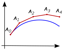
4 |
5 | ## Introduction
6 | This repository contains an implementation of the Euler method in the F# programming language. The Euler method is a simple numerical technique used for solving ordinary differential equations (ODEs) with an initial value problem. It is a first-order numerical method that approximates the solution by stepping through the solution space with small increments.
7 |
8 | ## Installation
9 | To run the provided code, ensure you have F# installed on your system. You can install F# using various methods depending on your operating system. Visit [F# Software Foundation](https://fsharp.org/use/) for installation instructions.
10 |
11 | ## Usage
12 | 1. Clone or download this repository to your local machine.
13 | 2. Navigate to the directory containing the code files.
14 | 3. Open a terminal or command prompt in that directory.
15 | 4. Execute the following command to compile and run the code:
16 |
17 | ```bash
18 | dotnet run
19 | ```
20 |
21 | 5. The program will output the solution to the ordinary differential equation (ODE) using the Euler method.
22 |
23 | ## Code Explanation
24 | ```fsharp
25 | open System
26 |
27 | // Function for solving an ordinary differential equation (EDO) using the Euler method
28 | let eulerMethod (f: float -> float -> float) (x0: float) (y0: float) (xf: float) (h: float) =
29 | let mutable x = x0
30 | let mutable y = y0
31 | let mutable values = []
32 |
33 | while x <= xf do
34 | values <- (x, y) :: values
35 | let slope = f x y
36 | y <- y + h * slope
37 | x <- x + h
38 |
39 | values |> List.rev
40 |
41 | // Example: Solve the ordinary differential equation (EDO) y' = -2y, y(0) = 1, for x in [0, 2] with step size h = 0.1
42 | let f x y = -2.0 * y
43 | let x0 = 0.0
44 | let y0 = 1.0
45 | let xf = 2.0
46 | let h = 0.1
47 |
48 | let solution = eulerMethod f x0 y0 xf h
49 | printfn "Solution:"
50 | solution |> List.iter (fun (x, y) -> printfn "x = %f, y = %f" x y)
51 | ```
52 |
53 | ## Example
54 |
55 | In this example, the code solves the ordinary differential equation (ODE) $y' = -2y$ with the initial condition $y(0) = 1$, for $x$ in the interval $[0, 2]$ with a step size $h = 0.1$ using the Euler method. The output provides the solution points $(x, y)$ along the solution curve.
56 |
57 | ## References
58 |
59 | The Organic Chemistry Tutor. (2017, 11 febrero). Euler’s Method Differential equations, examples, numerical methods, calculus [Video]. YouTube. https://www.youtube.com/watch?v=ukNbG7muKho
--------------------------------------------------------------------------------
/src/Fourier-transform/Fourier-transform.fsproj:
--------------------------------------------------------------------------------
1 |
2 |
3 |
4 | Exe
5 | net8.0
6 | Fourier_transform
7 |
8 |
9 |
10 |
11 |
12 |
13 |
14 |
--------------------------------------------------------------------------------
/src/Fourier-transform/Program.fs:
--------------------------------------------------------------------------------
1 | open System
2 | open System.Numerics
3 |
4 | // Function to calculate the Discrete Fourier Transform (DFT) of an array of complex numbers
5 |
6 | let discreteFourierTransform (input: Complex[]) =
7 | let n = input.Length
8 | let pi = 4.0 * atan 1.0
9 | Array.init n (fun k ->
10 | let mutable sum = Complex.Zero
11 | for j in 0 .. n - 1 do
12 | let angle = -2.0 * pi * float k * float j / float n
13 | let omega = Complex.FromPolarCoordinates(1.0, angle)
14 | sum <- sum + input.[j] * omega
15 | sum)
16 |
17 | // Function to print an array of complex numbers
18 | let printComplexArray (arr: Complex[]) =
19 | for i = 0 to arr.Length - 1 do
20 | printfn "%A" arr.[i]
21 |
22 | let inputData = [| Complex(1.0, 0.0); Complex(2.0, 0.0); Complex(3.0, 0.0); Complex(4.0, 0.0) |]
23 |
24 | printfn "Input Data:"
25 | printComplexArray inputData
26 |
27 | let result = discreteFourierTransform inputData
28 |
29 | printfn "Discrete Fourier Transform (DFT):"
30 | printComplexArray result
31 |
--------------------------------------------------------------------------------
/src/Fourier-transform/README.md:
--------------------------------------------------------------------------------
1 | # Fourier transform
2 |
3 | 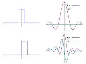
4 |
5 | ## Introduction
6 | This repository contains an implementation of the Fourier transform method in the F# programming language. The Fourier transform is a mathematical technique used to decompose a function of time (or a signal) into its constituent frequencies. It has applications in various fields, including signal processing, image processing, and quantum mechanics.
7 |
8 | ## Installation
9 | To run the provided code, ensure you have F# installed on your system. You can install F# using various methods depending on your operating system. Visit [F# Software Foundation](https://fsharp.org/use/) for installation instructions.
10 |
11 | ## Usage
12 | 1. Clone or download this repository to your local machine.
13 | 2. Navigate to the directory containing the code files.
14 | 3. Open a terminal or command prompt in that directory.
15 | 4. Execute the following command to compile and run the code:
16 |
17 | ```bash
18 | dotnet run
19 | ```
20 |
21 | ## Code explanation
22 |
23 | ```fsharp
24 | open System
25 | open System.Numerics
26 |
27 | // Function to calculate the Discrete Fourier Transform (DFT) of an array of complex numbers
28 | let discreteFourierTransform (input: Complex[]) =
29 | let n = input.Length
30 | let pi = 4.0 * atan 1.0
31 | Array.init n (fun k ->
32 | let mutable sum = Complex.Zero
33 | for j in 0 .. n - 1 do
34 | let angle = -2.0 * pi * float k * float j / float n
35 | let omega = Complex.FromPolarCoordinates(1.0, angle)
36 | sum <- sum + input.[j] * omega
37 | sum)
38 |
39 | // Function to print an array of complex numbers
40 | let printComplexArray (arr: Complex[]) =
41 | for i = 0 to arr.Length - 1 do
42 | printfn "%A" arr.[i]
43 |
44 | let inputData = [| Complex(1.0, 0.0); Complex(2.0, 0.0); Complex(3.0, 0.0); Complex(4.0, 0.0) |]
45 |
46 | printfn "Input Data:"
47 | printComplexArray inputData
48 |
49 | let result = discreteFourierTransform inputData
50 |
51 | printfn "Discrete Fourier Transform (DFT):"
52 | printComplexArray result
53 | ```
54 |
55 | ## Example
56 |
57 | In this example, the code calculates the Discrete Fourier Transform (DFT) of a set of input data represented as an array of complex numbers. The output provides the result of the DFT computati
58 |
59 |
60 | ## References
61 |
62 | Brian Douglas. (2013a, enero 11). Introduction to the Fourier Transform (Part 1) [Video]. YouTube. https://www.youtube.com/watch?v=1JnayXHhjlg
63 |
64 | Brian Douglas. (2013, 19 enero). Introduction to the Fourier Transform (Part 2) [Video]. YouTube. https://www.youtube.com/watch?v=kKu6JDqNma8
--------------------------------------------------------------------------------
/src/Gauss-seidel-method/Gauss-seidel-method.fsproj:
--------------------------------------------------------------------------------
1 |
2 |
3 |
4 | Exe
5 | net8.0
6 | Gauss_seidel_method
7 |
8 |
9 |
10 |
11 |
12 |
13 |
14 |
--------------------------------------------------------------------------------
/src/Gauss-seidel-method/Program.fs:
--------------------------------------------------------------------------------
1 | open System
2 |
3 | let printMatrix (matrix: float[][]) =
4 | for row in matrix do
5 | printfn "%A" row
6 |
7 | let printVector (vector: float[]) =
8 | printfn "%A" vector
9 |
10 | let gaussSeidelMethod (matrix: float[][]) (vector: float[]) (tolerance: float) (maxIterations: int) =
11 | let numRows = matrix.Length
12 | let numCols = matrix.[0].Length
13 | let mutable x = Array.zeroCreate(numCols)
14 | let mutable error = tolerance + 1.0
15 | let mutable iter = 0
16 |
17 | while iter < maxIterations && error > tolerance do
18 | let xOld = Array.copy x
19 | for i in 0 .. numRows - 1 do
20 | let mutable sum = vector.[i]
21 | for j in 0 .. numCols - 1 do
22 | if i <> j then
23 | sum <- sum - matrix.[i].[j] * x.[j]
24 | x.[i] <- sum / matrix.[i].[i]
25 | error <- Array.map2 (fun a b -> abs (a - b)) x xOld |> Array.max
26 | iter <- iter + 1
27 |
28 | if iter = maxIterations then
29 | printfn "Warning: Maximum number of iterations reached."
30 |
31 | x
32 |
33 | // Ejemplo de uso
34 | let matrix = [|[|10.0; 2.0; 1.0|]; [|1.0; 5.0; 1.0|]; [|2.0; 3.0; 10.0|]|]
35 | let vector = [|7.0; -8.0; 6.0|]
36 | let tolerance = 1e-6
37 | let maxIterations = 1000
38 |
39 | let solution = gaussSeidelMethod matrix vector tolerance maxIterations
40 | printfn "Solution:"
41 | printVector solution
42 |
--------------------------------------------------------------------------------
/src/Gauss-seidel-method/README.md:
--------------------------------------------------------------------------------
1 | # Gauss-Seidel Method
2 |
3 | 
4 |
5 | ## Introduction
6 | This repository contains an implementation of the Gauss-Seidel Method in the F# programming language. The Gauss-Seidel Method is an iterative technique used to solve a system of linear equations. It is a variant of the Jacobi Method and provides a faster convergence rate by using updated values of variables as soon as they are available.
7 |
8 | ## Installation
9 | To run the provided code, ensure you have F# installed on your system. You can install F# using various methods depending on your operating system. Visit [F# Software Foundation](https://fsharp.org/use/) for installation instructions.
10 |
11 | ## Usage
12 | 1. Clone or download this repository to your local machine.
13 | 2. Navigate to the directory containing the code files.
14 | 3. Open a terminal or command prompt in that directory.
15 | 4. Execute the following command to compile and run the code:
16 |
17 | ```bash
18 | dotnet run
19 | ```
20 |
21 | 5. The program will output the solution to the system of linear equations using the Gauss-Seidel Method.
22 |
23 | ## Code Explanation
24 | ```fsharp
25 | open System
26 |
27 | // Function to print a matrix
28 | let printMatrix (matrix: float[][]) =
29 | for row in matrix do
30 | printfn "%A" row
31 |
32 | // Function to print a vector
33 | let printVector (vector: float[]) =
34 | printfn "%A" vector
35 |
36 | // Gauss-Seidel Method implementation
37 | let gaussSeidelMethod (matrix: float[][]) (vector: float[]) (tolerance: float) (maxIterations: int) =
38 | let numRows = matrix.Length
39 | let numCols = matrix.[0].Length
40 | let mutable x = Array.zeroCreate(numCols)
41 | let mutable error = tolerance + 1.0
42 | let mutable iter = 0
43 |
44 | while iter < maxIterations && error > tolerance do
45 | let xOld = Array.copy x
46 | for i in 0 .. numRows - 1 do
47 | let mutable sum = vector.[i]
48 | for j in 0 .. numCols - 1 do
49 | if i <> j then
50 | sum <- sum - matrix.[i].[j] * x.[j]
51 | x.[i] <- sum / matrix.[i].[i]
52 | error <- Array.map2 (fun a b -> abs (a - b)) x xOld |> Array.max
53 | iter <- iter + 1
54 |
55 | if iter = maxIterations then
56 | printfn "Warning: Maximum number of iterations reached."
57 |
58 | x
59 |
60 | // Define the matrix and vector for the system of linear equations
61 | let matrix = [|[|10.0; 2.0; 1.0|]; [|1.0; 5.0; 1.0|]; [|2.0; 3.0; 10.0|]|]
62 | let vector = [|7.0; -8.0; 6.0|]
63 | let tolerance = 1e-6
64 | let maxIterations = 1000
65 |
66 | // Solve the system of linear equations using the Gauss-Seidel Method
67 | let solution = gaussSeidelMethod matrix vector tolerance maxIterations
68 | printfn "Solution:"
69 | printVector solution
70 | ```
71 |
72 | ## Example
73 |
74 | In this example, the code solves the following system of linear equations using the Gauss-Seidel Method:
75 |
76 | $10x_1 + 2x_2 + x_3 = 7$ \
77 | $x_1 + 5x_2 + x_3 = -8$ \
78 | $2x_1 + 3x_2 + 10x_3 = 6$
79 |
80 | The output provides the solution to the system of equations.
81 |
82 | ## References
83 |
84 | Jeffrey Chasnov. (2021b, febrero 10). Jacobi, Gauss-Seidel and SOR Methods | Lecture 66 | Numerical Methods for Engineers [Video]. YouTube. https://www.youtube.com/watch?v=QpzOttega9s
--------------------------------------------------------------------------------
/src/Gaussian-elimination/Gaussian-elimination.fsproj:
--------------------------------------------------------------------------------
1 |
2 |
3 |
4 | Exe
5 | net8.0
6 | Gaussian_elimination
7 |
8 |
9 |
10 |
11 |
12 |
13 |
14 |
--------------------------------------------------------------------------------
/src/Gaussian-elimination/Program.fs:
--------------------------------------------------------------------------------
1 | open System
2 |
3 | let printVector (vector: float[]) =
4 | printfn "%A" vector
5 |
6 | let gaussianElimination (matrix: float[][]) (vector: float[]) =
7 | let numRows = matrix.Length
8 | let numCols = matrix.[0].Length
9 | let augmentedMatrix = Array.zeroCreate(numRows)
10 |
11 | // Convert the Matrix to an Augmented Matrix with the Vector
12 | for i in 0 .. numRows - 1 do
13 | augmentedMatrix.[i] <- Array.append matrix.[i] [|vector.[i]|]
14 |
15 | // Forward Disposal
16 | for k in 0 .. numRows - 1 do
17 | for i in k + 1 .. numRows - 1 do
18 | let factor = augmentedMatrix.[i].[k] / augmentedMatrix.[k].[k]
19 | for j in k .. numCols do
20 | augmentedMatrix.[i].[j] <- augmentedMatrix.[i].[j] - factor * augmentedMatrix.[k].[j]
21 |
22 | // Backward Replacement
23 | let solution = Array.zeroCreate(numRows)
24 | for i in (numRows - 1) .. -1 .. 0 do
25 | let mutable sum = 0.0
26 | for j in (i + 1) .. numCols - 1 do
27 | sum <- sum + augmentedMatrix.[i].[j] * solution.[j]
28 | solution.[i] <- (augmentedMatrix.[i].[numCols - 1] - sum) / augmentedMatrix.[i].[i]
29 |
30 | solution
31 |
32 |
33 | // Ejemplo de uso
34 | let coefficients = [|[|2.0; 1.0; -1.0|]; [|1.0; 1.0; 1.0|]; [|1.0; -1.0; 2.0|]|]
35 | let constants = [|8.0; 12.0; 3.0|]
36 |
37 | printfn "Coefficients:"
38 | for i in 0 .. coefficients.Length - 1 do
39 | printVector coefficients.[i]
40 |
41 | printfn "Constants:"
42 | printVector constants
43 |
44 | let solution = gaussianElimination coefficients constants
45 | printfn "Solution:"
46 | printVector solution
47 |
--------------------------------------------------------------------------------
/src/Gaussian-elimination/README.md:
--------------------------------------------------------------------------------
1 | # Gaussian elimination method
2 |
3 | 
4 |
5 | ## Introduction
6 | This repository contains an implementation of Gaussian Elimination in the F# programming language. Gaussian Elimination is a method used to solve a system of linear equations by transforming the augmented matrix of coefficients and constants into row-echelon form through a series of elementary row operations.
7 |
8 | ## Installation
9 | To run the provided code, ensure you have F# installed on your system. You can install F# using various methods depending on your operating system. Visit [F# Software Foundation](https://fsharp.org/use/) for installation instructions.
10 |
11 | ## Usage
12 | 1. Clone or download this repository to your local machine.
13 | 2. Navigate to the directory containing the code files.
14 | 3. Open a terminal or command prompt in that directory.
15 | 4. Execute the following command to compile and run the code:
16 |
17 | ```bash
18 | dotnet run
19 | ```
20 |
21 | 5. The program will output the solution to the system of linear equations using Gaussian Elimination.
22 |
23 | ## Code Explanation
24 | ```fsharp
25 | open System
26 |
27 | // Function to print a vector
28 | let printVector (vector: float[]) =
29 | printfn "%A" vector
30 |
31 | // Gaussian Elimination implementation
32 | let gaussianElimination (matrix: float[][]) (vector: float[]) =
33 | let numRows = matrix.Length
34 | let numCols = matrix.[0].Length
35 | let augmentedMatrix = Array.zeroCreate(numRows)
36 |
37 | // Convert the Matrix to an Augmented Matrix with the Vector
38 | for i in 0 .. numRows - 1 do
39 | augmentedMatrix.[i] <- Array.append matrix.[i] [|vector.[i]|]
40 |
41 | // Forward Disposal
42 | for k in 0 .. numRows - 1 do
43 | for i in k + 1 .. numRows - 1 do
44 | let factor = augmentedMatrix.[i].[k] / augmentedMatrix.[k].[k]
45 | for j in k .. numCols do
46 | augmentedMatrix.[i].[j] <- augmentedMatrix.[i].[j] - factor * augmentedMatrix.[k].[j]
47 |
48 | // Backward Replacement
49 | let solution = Array.zeroCreate(numRows)
50 | for i in (numRows - 1) .. -1 .. 0 do
51 | let mutable sum = 0.0
52 | for j in (i + 1) .. numCols - 1 do
53 | sum <- sum + augmentedMatrix.[i].[j] * solution.[j]
54 | solution.[i] <- (augmentedMatrix.[i].[numCols - 1] - sum) / augmentedMatrix.[i].[i]
55 |
56 | solution
57 |
58 | // Define the coefficients matrix and constants vector for the system of linear equations
59 | let coefficients = [|[|2.0; 1.0; -1.0|]; [|1.0; 1.0; 1.0|]; [|1.0; -1.0; 2.0|]|]
60 | let constants = [|8.0; 12.0; 3.0|]
61 |
62 | printfn "Coefficients:"
63 | for i in 0 .. coefficients.Length - 1 do
64 | printVector coefficients.[i]
65 |
66 | printfn "Constants:"
67 | printVector constants
68 |
69 | // Solve the system of linear equations using Gaussian Elimination
70 | let solution = gaussianElimination coefficients constants
71 | printfn "Solution:"
72 | printVector solution
73 | ```
74 |
75 | ## Example
76 |
77 | Example
78 | In this example, the code solves the following system of linear equations using Gaussian Elimination:
79 |
80 | $2x_1 + x_2 + x_3 = 8$ \
81 | $x_1 + x_2 + x_3 = 12$ \
82 | $x_1 + x_2 + 2x_3 = 3$
83 |
84 | The output provides the solution to the system of equations.
85 |
86 | ## References
87 |
88 | The Organic Chemistry Tutor. (2018a, febrero 18). Gaussian elimination & Row echelon form [Video]. YouTube. https://www.youtube.com/watch?v=eDb6iugi6Uk
89 |
90 |
--------------------------------------------------------------------------------
/src/Gradient-descent/Gradient-descent.fsproj:
--------------------------------------------------------------------------------
1 |
2 |
3 |
4 | Exe
5 | net8.0
6 | Gradient_descent
7 |
8 |
9 |
10 |
11 |
12 |
13 |
14 |
--------------------------------------------------------------------------------
/src/Gradient-descent/Program.fs:
--------------------------------------------------------------------------------
1 | open System
2 |
3 | // Define the cost function
4 | let costFunction (theta0: float) (theta1: float) (xValues: float[]) (yValues: float[]) =
5 | let m = float xValues.Length
6 | let sumOfSquares = Array.map2 (fun x y -> (theta0 + theta1 * x - y) ** 2.0) xValues yValues |> Array.sum
7 | sumOfSquares / (2.0 * m)
8 |
9 | // Calculate the partial derivative of the cost function with respect to theta0
10 | let partialDerivativeTheta0 (theta0: float) (theta1: float) (xValues: float[]) (yValues: float[]) =
11 | let m = float xValues.Length
12 | let sum = Array.map2 (fun x y -> theta0 + theta1 * x - y) xValues yValues |> Array.sum
13 | sum / m
14 |
15 | // Calculate the partial derivative of the cost function with respect to theta1
16 | let partialDerivativeTheta1 (theta0: float) (theta1: float) (xValues: float[]) (yValues: float[]) =
17 | let m = float xValues.Length
18 | let sum = Array.map2 (fun x y -> (theta0 + theta1 * x - y) * x) xValues yValues |> Array.sum
19 | sum / m
20 |
21 | // Gradient descent algorithm
22 | let gradientDescent (xValues: float[]) (yValues: float[]) (alpha: float) (iterations: int) =
23 | let mutable theta0 = 0.0
24 | let mutable theta1 = 0.0
25 |
26 | for i in 1 .. iterations do
27 | let tempTheta0 = theta0 - alpha * partialDerivativeTheta0 theta0 theta1 xValues yValues
28 | let tempTheta1 = theta1 - alpha * partialDerivativeTheta1 theta0 theta1 xValues yValues
29 | theta0 <- tempTheta0
30 | theta1 <- tempTheta1
31 |
32 | theta0, theta1
33 |
34 | let xValues = [|1.0; 2.0; 3.0; 4.0; 5.0|]
35 | let yValues = [|2.0; 3.0; 4.0; 5.0; 6.0|]
36 | let alpha = 0.01
37 | let iterations = 1000
38 |
39 | let theta0Optimal, theta1Optimal = gradientDescent xValues yValues alpha iterations
40 |
41 | printfn "Optimal theta0: %f" theta0Optimal
42 | printfn "Optimal theta1: %f" theta1Optimal
43 |
--------------------------------------------------------------------------------
/src/Gradient-descent/README.md:
--------------------------------------------------------------------------------
1 | # Gradient descent
2 |
3 | 
4 |
5 | ## Introduction
6 | This repository contains an implementation of the Gradient Descent method in the F# programming language. Gradient Descent is an optimization algorithm used to minimize the cost function of a model by iteratively adjusting its parameters. In this implementation, we apply the Gradient Descent method to find the optimal parameters for a linear regression model.
7 |
8 | ## Installation
9 | To run the provided code, ensure you have F# installed on your system. You can install F# using various methods depending on your operating system. Visit [F# Software Foundation](https://fsharp.org/use/) for installation instructions.
10 |
11 | ## Usage
12 | 1. Clone or download this repository to your local machine.
13 | 2. Navigate to the directory containing the code files.
14 | 3. Open a terminal or command prompt in that directory.
15 | 4. Execute the following command to compile and run the code:
16 |
17 | ```bash
18 | dotnet run
19 | ```
20 |
21 | ## Code explanation
22 |
23 | ```fsharp
24 | open System
25 |
26 | // Define the cost function
27 | let costFunction (theta0: float) (theta1: float) (xValues: float[]) (yValues: float[]) =
28 | let m = float xValues.Length
29 | let sumOfSquares = Array.map2 (fun x y -> (theta0 + theta1 * x - y) ** 2.0) xValues yValues |> Array.sum
30 | sumOfSquares / (2.0 * m)
31 |
32 | // Calculate the partial derivative of the cost function with respect to theta0
33 | let partialDerivativeTheta0 (theta0: float) (theta1: float) (xValues: float[]) (yValues: float[]) =
34 | let m = float xValues.Length
35 | let sum = Array.map2 (fun x y -> theta0 + theta1 * x - y) xValues yValues |> Array.sum
36 | sum / m
37 |
38 | // Calculate the partial derivative of the cost function with respect to theta1
39 | let partialDerivativeTheta1 (theta0: float) (theta1: float) (xValues: float[]) (yValues: float[]) =
40 | let m = float xValues.Length
41 | let sum = Array.map2 (fun x y -> (theta0 + theta1 * x - y) * x) xValues yValues |> Array.sum
42 | sum / m
43 |
44 | // Gradient descent algorithm
45 | let gradientDescent (xValues: float[]) (yValues: float[]) (alpha: float) (iterations: int) =
46 | let mutable theta0 = 0.0
47 | let mutable theta1 = 0.0
48 |
49 | for i in 1 .. iterations do
50 | let tempTheta0 = theta0 - alpha * partialDerivativeTheta0 theta0 theta1 xValues yValues
51 | let tempTheta1 = theta1 - alpha * partialDerivativeTheta1 theta0 theta1 xValues yValues
52 | theta0 <- tempTheta0
53 | theta1 <- tempTheta1
54 |
55 | theta0, theta1
56 |
57 | let xValues = [|1.0; 2.0; 3.0; 4.0; 5.0|]
58 | let yValues = [|2.0; 3.0; 4.0; 5.0; 6.0|]
59 | let alpha = 0.01
60 | let iterations = 1000
61 |
62 | let theta0Optimal, theta1Optimal = gradientDescent xValues yValues alpha iterations
63 |
64 | printfn "Optimal theta0: %f" theta0Optimal
65 | printfn "Optimal theta1: %f" theta1Optimal
66 | ```
67 |
68 |
69 | ## Example
70 |
71 |
72 | In this example, the code estimates the optimal parameters \( \theta_0 \) and \( \theta_1 \) for a linear regression model using the Gradient Descent method. The output provides the optimal values of \( \theta_0 \) and \( \theta_1 \) obtained after a specified number of iterations.
73 |
74 | ## References
75 |
76 | IBM Technology. (2022, 15 septiembre). Gradient Descent explained [Vídeo]. YouTube. https://www.youtube.com/watch?v=i62czvwDlsw
--------------------------------------------------------------------------------
/src/Jacobi-method/Jacobi-method.fsproj:
--------------------------------------------------------------------------------
1 |
2 |
3 |
4 | Exe
5 | net8.0
6 | Jacobi_method
7 |
8 |
9 |
10 |
11 |
12 |
13 |
14 |
--------------------------------------------------------------------------------
/src/Jacobi-method/Program.fs:
--------------------------------------------------------------------------------
1 | open System
2 |
3 | let printMatrix (matrix: float[][]) =
4 | for row in matrix do
5 | printfn "%A" row
6 |
7 | let printVector (vector: float[]) =
8 | printfn "%A" vector
9 |
10 | let jacobiMethod (matrix: float[][]) (vector: float[]) (tolerance: float) (maxIterations: int) =
11 | let numRows = matrix.Length
12 | let numCols = matrix.[0].Length
13 | let mutable x = Array.zeroCreate(numCols)
14 | let mutable error = tolerance + 1.0
15 | let mutable iter = 0
16 |
17 | while iter < maxIterations && error > tolerance do
18 | let xOld = Array.copy x
19 | for i in 0 .. numRows - 1 do
20 | let mutable sum = vector.[i]
21 | for j in 0 .. numCols - 1 do
22 | if i <> j then
23 | sum <- sum - matrix.[i].[j] * xOld.[j]
24 | x.[i] <- sum / matrix.[i].[i]
25 | error <- Array.map2 (fun a b -> abs (a - b)) x xOld |> Array.max
26 | iter <- iter + 1
27 |
28 | if iter = maxIterations then
29 | printfn "Warning: Maximum number of iterations reached."
30 |
31 | x
32 |
33 | let matrix = [|[|10.0; 2.0; 1.0|]; [|1.0; 5.0; 1.0|]; [|2.0; 3.0; 10.0|]|]
34 | let vector = [|7.0; -8.0; 6.0|]
35 | let tolerance = 1e-6
36 | let maxIterations = 1000
37 |
38 | let solution = jacobiMethod matrix vector tolerance maxIterations
39 | printfn "Solution:"
40 | printVector solution
41 |
--------------------------------------------------------------------------------
/src/Jacobi-method/README.md:
--------------------------------------------------------------------------------
1 | # Jacobi method
2 |
3 | 
4 |
5 | ## Introduction
6 | This repository contains an implementation of the Jacobi Method in the F# programming language. The Jacobi Method is an iterative technique used to solve a system of linear equations, particularly when the matrix of the system is diagonally dominant. It iteratively improves an initial guess to approximate the solution.
7 |
8 | ## Installation
9 | To run the provided code, ensure you have F# installed on your system. You can install F# using various methods depending on your operating system. Visit [F# Software Foundation](https://fsharp.org/use/) for installation instructions.
10 |
11 | ## Usage
12 | 1. Clone or download this repository to your local machine.
13 | 2. Navigate to the directory containing the code files.
14 | 3. Open a terminal or command prompt in that directory.
15 | 4. Execute the following command to compile and run the code:
16 |
17 | ```bash
18 | dotnet run
19 | ```
20 |
21 | 5. The program will output the solution to the system of linear equations using the Jacobi Method.
22 |
23 | ## Code Explanation
24 | ```fsharp
25 | open System
26 |
27 | // Function to print a matrix
28 | let printMatrix (matrix: float[][]) =
29 | for row in matrix do
30 | printfn "%A" row
31 |
32 | // Function to print a vector
33 | let printVector (vector: float[]) =
34 | printfn "%A" vector
35 |
36 | // Jacobi Method implementation
37 | let jacobiMethod (matrix: float[][]) (vector: float[]) (tolerance: float) (maxIterations: int) =
38 | let numRows = matrix.Length
39 | let numCols = matrix.[0].Length
40 | let mutable x = Array.zeroCreate(numCols)
41 | let mutable error = tolerance + 1.0
42 | let mutable iter = 0
43 |
44 | while iter < maxIterations && error > tolerance do
45 | let xOld = Array.copy x
46 | for i in 0 .. numRows - 1 do
47 | let mutable sum = vector.[i]
48 | for j in 0 .. numCols - 1 do
49 | if i <> j then
50 | sum <- sum - matrix.[i].[j] * xOld.[j]
51 | x.[i] <- sum / matrix.[i].[i]
52 | error <- Array.map2 (fun a b -> abs (a - b)) x xOld |> Array.max
53 | iter <- iter + 1
54 |
55 | if iter = maxIterations then
56 | printfn "Warning: Maximum number of iterations reached."
57 |
58 | x
59 |
60 | // Define the matrix and vector for the system of linear equations
61 | let matrix = [|[|10.0; 2.0; 1.0|]; [|1.0; 5.0; 1.0|]; [|2.0; 3.0; 10.0|]|]
62 | let vector = [|7.0; -8.0; 6.0|]
63 | let tolerance = 1e-6
64 | let maxIterations = 1000
65 |
66 | // Solve the system of linear equations using the Jacobi Method
67 | let solution = jacobiMethod matrix vector tolerance maxIterations
68 | printfn "Solution:"
69 | printVector solution
70 | ```
71 |
72 | ## Example
73 |
74 | In this example, the code solves the following system of linear equations using the Jacobi Method:
75 |
76 | $10x_1 + 2x_2 + x_3 = 7$ \
77 | $x_1 + 5x_2 + x_3 = -8$ \
78 | $2x_1 + 3x_2 + 10x_3 = 6$
79 |
80 | The output provides the solution to the system of equations.
81 |
82 | ## References
83 |
84 | Jeffrey Chasnov. (2021b, febrero 10). Jacobi, Gauss-Seidel and SOR Methods | Lecture 66 | Numerical Methods for Engineers [Video]. YouTube. https://www.youtube.com/watch?v=QpzOttega9s
85 |
86 |
87 |
--------------------------------------------------------------------------------
/src/LU-decomposition/LU-decomposition.fsproj:
--------------------------------------------------------------------------------
1 |
2 |
3 |
4 | Exe
5 | net8.0
6 | LU_decomposition
7 |
8 |
9 |
10 |
11 |
12 |
13 |
14 |
--------------------------------------------------------------------------------
/src/LU-decomposition/Program.fs:
--------------------------------------------------------------------------------
1 | open System
2 |
3 | let printMatrix (matrix: float[][]) =
4 | for row in matrix do
5 | printfn "%A" row
6 |
7 | // Function to perform LU decomposition
8 | let luDecomposition (matrix: float[][]) =
9 | let numRows = matrix.Length
10 | let numCols = matrix.[0].Length
11 | let lower = Array.zeroCreate(numRows)
12 | let upper = Array.zeroCreate(numRows)
13 |
14 | for i in 0 .. numRows - 1 do
15 | lower.[i] <- Array.zeroCreate(numRows)
16 | upper.[i] <- Array.zeroCreate(numCols)
17 |
18 | // Fill the upper and diagonal matrix of lower
19 | for i in 0 .. numRows - 1 do
20 | // Fill the upper matrix
21 | for j in i .. numCols - 1 do
22 | upper.[i].[j] <- matrix.[i].[j]
23 |
24 | // Fill the diagonal of lower
25 | lower.[i].[i] <- 1.0
26 |
27 | // Perform LU decomposition
28 | for i in 0 .. numRows - 1 do
29 | for j in i + 1 .. numRows - 1 do
30 | let factor = upper.[j].[i] / upper.[i].[i]
31 | lower.[j].[i] <- factor
32 | for k in i .. numCols - 1 do
33 | upper.[j].[k] <- upper.[j].[k] - factor * upper.[i].[k]
34 |
35 | lower, upper
36 |
37 | let coefficients = [|[|2.0; 1.0; -1.0|]; [|1.0; 1.0; 1.0|]; [|1.0; -1.0; 2.0|]|]
38 | printfn "Coefficients:"
39 | printMatrix coefficients
40 |
41 |
42 | let lower, upper = luDecomposition coefficients
43 | printfn "Lower:"
44 | printMatrix lower
45 | printfn "Upper:"
46 | printMatrix upper
47 |
--------------------------------------------------------------------------------
/src/LU-decomposition/README.md:
--------------------------------------------------------------------------------
1 | # LU decomposition
2 |
3 | 
4 |
5 | ## Introduction
6 | This repository contains an implementation of LU Decomposition in the F# programming language. LU Decomposition, also known as LU factorization, is a method used to factorize a matrix into the product of a lower triangular matrix (L) and an upper triangular matrix (U). It is commonly used in solving systems of linear equations and in numerical analysis.
7 |
8 | ## Installation
9 | To run the provided code, ensure you have F# installed on your system. You can install F# using various methods depending on your operating system. Visit [F# Software Foundation](https://fsharp.org/use/) for installation instructions.
10 |
11 | ## Usage
12 | 1. Clone or download this repository to your local machine.
13 | 2. Navigate to the directory containing the code files.
14 | 3. Open a terminal or command prompt in that directory.
15 | 4. Execute the following command to compile and run the code:
16 |
17 | ```bash
18 | dotnet run
19 | ```
20 |
21 | 5. The program will output the lower triangular matrix (L) and upper triangular matrix (U) resulting from LU decomposition of the input matrix.
22 |
23 | ## Code Explanation
24 | ```fsharp
25 | open System
26 |
27 | // Function to print a matrix
28 | let printMatrix (matrix: float[][]) =
29 | for row in matrix do
30 | printfn "%A" row
31 |
32 | // Function to perform LU decomposition
33 | let luDecomposition (matrix: float[][]) =
34 | let numRows = matrix.Length
35 | let numCols = matrix.[0].Length
36 | let lower = Array.zeroCreate(numRows)
37 | let upper = Array.zeroCreate(numRows)
38 |
39 | for i in 0 .. numRows - 1 do
40 | lower.[i] <- Array.zeroCreate(numRows)
41 | upper.[i] <- Array.zeroCreate(numCols)
42 |
43 | // Fill the upper and diagonal matrix of lower
44 | for i in 0 .. numRows - 1 do
45 | // Fill the upper matrix
46 | for j in i .. numCols - 1 do
47 | upper.[i].[j] <- matrix.[i].[j]
48 |
49 | // Fill the diagonal of lower
50 | lower.[i].[i] <- 1.0
51 |
52 | // Perform LU decomposition
53 | for i in 0 .. numRows - 1 do
54 | for j in i + 1 .. numRows - 1 do
55 | let factor = upper.[j].[i] / upper.[i].[i]
56 | lower.[j].[i] <- factor
57 | for k in i .. numCols - 1 do
58 | upper.[j].[k] <- upper.[j].[k] - factor * upper.[i].[k]
59 |
60 | lower, upper
61 |
62 | // Define the coefficients matrix for LU decomposition
63 | let coefficients = [|[|2.0; 1.0; -1.0|]; [|1.0; 1.0; 1.0|]; [|1.0; -1.0; 2.0|]|]
64 | printfn "Coefficients:"
65 | printMatrix coefficients
66 |
67 | // Perform LU decomposition
68 | let lower, upper = luDecomposition coefficients
69 | printfn "Lower:"
70 | printMatrix lower
71 | printfn "Upper:"
72 | printMatrix upper
73 | ```
74 |
75 | ## Example
76 |
77 | In this example, the code performs LU Decomposition on the following coefficient matrix:
78 |
79 | 2.0 1.0 -1.0 \
80 | 1.0 1.0 1.0 \
81 | 1.0 -1.0 2.0
82 |
83 | The output provides the lower triangular matrix (L) and upper triangular matrix (U) resulting from the LU decomposition.
84 |
85 | ## References
86 |
87 | MIT OpenCourseWare. (2018, 25 julio). LU decomposition [Video]. YouTube. https://www.youtube.com/watch?v=-eA2D_rIcNA
--------------------------------------------------------------------------------
/src/Linear-interpolation-method/Linear-interpolation-method.fsproj:
--------------------------------------------------------------------------------
1 |
2 |
3 |
4 | Exe
5 | net8.0
6 | Linear_interpolation_method
7 |
8 |
9 |
10 |
11 |
12 |
13 |
14 |
--------------------------------------------------------------------------------
/src/Linear-interpolation-method/Program.fs:
--------------------------------------------------------------------------------
1 | open System
2 |
3 | // Linear interpolation method
4 | let linearInterpolation (xValues: float[]) (yValues: float[]) (x: float) =
5 | let rec findSegment i =
6 | if i = xValues.Length - 1 || xValues.[i + 1] >= x then i
7 | else findSegment (i + 1)
8 |
9 | let segmentIndex = findSegment 0
10 | let x0, y0 = xValues.[segmentIndex], yValues.[segmentIndex]
11 | let x1, y1 = xValues.[segmentIndex + 1], yValues.[segmentIndex + 1]
12 |
13 | let slope = (y1 - y0) / (x1 - x0)
14 | let intercept = y0 - slope * x0
15 | slope * x + intercept
16 |
17 | let xValues = [|1.0; 2.0; 3.0; 4.0; 5.0|]
18 | let yValues = [|2.0; 3.0; 5.0; 7.0; 11.0|]
19 | let x = 2.5
20 |
21 | let y = linearInterpolation xValues yValues x
22 |
23 | printfn "Interpolated value at x = %f is y = %f" x y
24 |
--------------------------------------------------------------------------------
/src/Linear-interpolation-method/README.md:
--------------------------------------------------------------------------------
1 | # Linear interpolation method
2 |
3 | 
4 |
5 | ## Introduction
6 | This repository contains an implementation of the linear interpolation method in the F# programming language. Linear interpolation is a simple and commonly used technique for estimating values between two known data points. It assumes a linear relationship between the data points and provides an approximation for intermediate values.
7 |
8 | ## Installation
9 | To run the provided code, ensure you have F# installed on your system. You can install F# using various methods depending on your operating system. Visit [F# Software Foundation](https://fsharp.org/use/) for installation instructions.
10 |
11 | ## Usage
12 | 1. Clone or download this repository to your local machine.
13 | 2. Navigate to the directory containing the code files.
14 | 3. Open a terminal or command prompt in that directory.
15 | 4. Execute the following command to compile and run the code:
16 |
17 | ```bash
18 | dotnet run
19 | ```
20 |
21 | 5. The program will output the interpolated value at the specified point `x`.
22 |
23 | ## Code Explanation
24 | ```fsharp
25 | open System
26 |
27 | // Linear interpolation method
28 | let linearInterpolation (xValues: float[]) (yValues: float[]) (x: float) =
29 | let rec findSegment i =
30 | if i = xValues.Length - 1 || xValues.[i + 1] >= x then i
31 | else findSegment (i + 1)
32 |
33 | let segmentIndex = findSegment 0
34 | let x0, y0 = xValues.[segmentIndex], yValues.[segmentIndex]
35 | let x1, y1 = xValues.[segmentIndex + 1], yValues.[segmentIndex + 1]
36 |
37 | let slope = (y1 - y0) / (x1 - x0)
38 | let intercept = y0 - slope * x0
39 | slope * x + intercept
40 |
41 | // Example data
42 | let xValues = [|1.0; 2.0; 3.0; 4.0; 5.0|]
43 | let yValues = [|2.0; 3.0; 5.0; 7.0; 11.0|]
44 | let x = 2.5
45 |
46 | // Perform linear interpolation
47 | let y = linearInterpolation xValues yValues x
48 |
49 | printfn "Interpolated value at x = %f is y = %f" x y
50 | ```
51 |
52 | ## Example
53 |
54 | In this example, the code performs linear interpolation on the given data points to estimate the value of \( y \) at \( x = 2.5 \). The output provides the interpolated value at the specified point.
55 |
56 | ## References
57 |
58 | Jeffrey Chasnov. (2021c, febrero 10). Interpolation | Lecture 43 | Numerical Methods for Engineers [Video]. YouTube. https://www.youtube.com/watch?v=RpxoN9-i7Jc
--------------------------------------------------------------------------------
/src/Linear-regression-method/Linear-regression-method.fsproj:
--------------------------------------------------------------------------------
1 |
2 |
3 |
4 | Exe
5 | net8.0
6 | Linear_regression_method
7 |
8 |
9 |
10 |
11 |
12 |
13 |
14 |
--------------------------------------------------------------------------------
/src/Linear-regression-method/Program.fs:
--------------------------------------------------------------------------------
1 | open System
2 |
3 | // Minimum squares method
4 | let linearRegression (xValues: float[]) (yValues: float[]) =
5 | let n = float xValues.Length
6 | let sumX = Array.sum xValues
7 | let sumY = Array.sum yValues
8 | let sumXY = Array.map2 (*) xValues yValues |> Array.sum
9 | let sumXSquare = Array.map (fun x -> x * x) xValues |> Array.sum
10 | let meanX = sumX / n
11 | let meanY = sumY / n
12 |
13 | let slope = (n * sumXY - sumX * sumY) / (n * sumXSquare - sumX * sumX)
14 | let intercept = meanY - slope * meanX
15 |
16 | slope, intercept
17 |
18 | let xValues = [|1.0; 2.0; 3.0; 4.0; 5.0|]
19 | let yValues = [|2.0; 3.0; 4.0; 5.0; 6.0|]
20 |
21 | let slope, intercept = linearRegression xValues yValues
22 |
23 | printfn "Slope: %f" slope
24 | printfn "Intercept: %f" intercept
25 |
--------------------------------------------------------------------------------
/src/Linear-regression-method/README.md:
--------------------------------------------------------------------------------
1 | # Linear regression method
2 |
3 | 
4 |
5 | ## Introduction
6 | This repository contains an implementation of the linear regression method in the F# programming language. Linear regression is a statistical method used to model the relationship between two variables by fitting a linear equation to observed data.
7 |
8 | ## Installation
9 | To run the provided code, ensure you have F# installed on your system. You can install F# using various methods depending on your operating system. Visit [F# Software Foundation](https://fsharp.org/use/) for installation instructions.
10 |
11 | ## Usage
12 | 1. Clone or download this repository to your local machine.
13 | 2. Navigate to the directory containing the code files.
14 | 3. Open a terminal or command prompt in that directory.
15 | 4. Execute the following command to compile and run the code:
16 |
17 | ```bash
18 | dotnet run
19 | ```
20 |
21 | 5. The program will output the slope and intercept of the linear regression line.
22 |
23 | ## Code explanation
24 |
25 | ```fsharp
26 | open System
27 |
28 | // Minimum squares method
29 | let linearRegression (xValues: float[]) (yValues: float[]) =
30 | // Calculate the number of data points
31 | let n = float xValues.Length
32 | // Calculate the sum of x and y values
33 | let sumX = Array.sum xValues
34 | let sumY = Array.sum yValues
35 | // Calculate the sum of products of x and y values
36 | let sumXY = Array.map2 (*) xValues yValues |> Array.sum
37 | // Calculate the sum of squared x values
38 | let sumXSquare = Array.map (fun x -> x * x) xValues |> Array.sum
39 | // Calculate the mean of x and y values
40 | let meanX = sumX / n
41 | let meanY = sumY / n
42 |
43 | // Calculate the slope and intercept of the linear regression line
44 | let slope = (n * sumXY - sumX * sumY) / (n * sumXSquare - sumX * sumX)
45 | let intercept = meanY - slope * meanX
46 |
47 | slope, intercept
48 |
49 | // Example data points
50 | let xValues = [|1.0; 2.0; 3.0; 4.0; 5.0|]
51 | let yValues = [|2.0; 3.0; 4.0; 5.0; 6.0|]
52 |
53 | // Perform linear regression on the example data points
54 | let slope, intercept = linearRegression xValues yValues
55 |
56 | // Output the results
57 | printfn "Slope: %f" slope
58 | printfn "Intercept: %f" intercept
59 | ```
60 |
61 | ## Example
62 |
63 | In this example, the code performs linear regression on the given data points to estimate the slope and intercept of the linear regression line. The output provides the calculated slope and intercept values.
64 |
65 | ## References
66 |
67 | The Organic Chemistry Tutor. (2020, 14 julio). Linear Regression Using Least Squares Method - Line of Best Fit Equation [Video]. YouTube. https://www.youtube.com/watch?v=P8hT5nDai6A
--------------------------------------------------------------------------------
/src/Monte-carlo-method-for-PI/Monte-carlo-method-for-PI.fsproj:
--------------------------------------------------------------------------------
1 |
2 |
3 |
4 | Exe
5 | net8.0
6 | Monte_carlo_method_for_PI
7 |
8 |
9 |
10 |
11 |
12 |
13 |
14 |
--------------------------------------------------------------------------------
/src/Monte-carlo-method-for-PI/Program.fs:
--------------------------------------------------------------------------------
1 | open System
2 |
3 | // Function to estimate the value of π using the Monte Carlo method
4 |
5 | let monteCarloPiEstimation (numPoints: int) =
6 | let rand = System.Random()
7 | let mutable numPointsInsideCircle = 0
8 |
9 | for _ in 1 .. numPoints do
10 | let x = rand.NextDouble()
11 | let y = rand.NextDouble()
12 | if x * x + y * y <= 1.0 then
13 | numPointsInsideCircle <- numPointsInsideCircle + 1
14 |
15 | let piEstimation = 4.0 * float numPointsInsideCircle / float numPoints
16 | piEstimation
17 |
18 | // Calculate the value of π using the Monte Carlo method with 1,000,000 points
19 |
20 | let numPoints = 1000000
21 | let estimatedPi = monteCarloPiEstimation numPoints
22 |
23 | printfn "The estimated value of π using the Monte Carlo method with %d points is approximately %f" numPoints estimatedPi
24 |
--------------------------------------------------------------------------------
/src/Monte-carlo-method-for-PI/README.md:
--------------------------------------------------------------------------------
1 | # Monte Carlo Method for π
2 |
3 | 
4 |
5 |
6 | ## Introduction
7 | This repository contains an implementation of the Monte Carlo method in the F# programming language to estimate the value of π (pi). The Monte Carlo method is a statistical technique that uses random sampling to obtain numerical results. In this implementation, we use the method to estimate π by generating random points within a square and determining the proportion that fall within a quarter of a unit circle.
8 |
9 | ## Installation
10 | To run the provided code, ensure you have F# installed on your system. You can install F# using various methods depending on your operating system. Visit [F# Software Foundation](https://fsharp.org/use/) for installation instructions.
11 |
12 | ## Usage
13 | 1. Clone or download this repository to your local machine.
14 | 2. Navigate to the directory containing the code files.
15 | 3. Open a terminal or command prompt in that directory.
16 | 4. Execute the following command to compile and run the code:
17 |
18 | ```bash
19 | dotnet run
20 | ```
21 |
22 | ## Code explanation
23 |
24 | ```fsharp
25 | open System
26 |
27 | // Function to estimate the value of π using the Monte Carlo method
28 | let monteCarloPiEstimation (numPoints: int) =
29 | let rand = System.Random()
30 | let mutable numPointsInsideCircle = 0
31 |
32 | for _ in 1 .. numPoints do
33 | let x = rand.NextDouble()
34 | let y = rand.NextDouble()
35 | if x * x + y * y <= 1.0 then
36 | numPointsInsideCircle <- numPointsInsideCircle + 1
37 |
38 | let piEstimation = 4.0 * float numPointsInsideCircle / float numPoints
39 | piEstimation
40 |
41 | // Calculate the value of π using the Monte Carlo method with 1,000,000 points
42 | let numPoints = 1000000
43 | let estimatedPi = monteCarloPiEstimation numPoints
44 |
45 | printfn "The estimated value of π using the Monte Carlo method with %d points is approximately %f" numPoints estimatedPi
46 | ```
47 |
48 | ## Example
49 |
50 | In this example, the code estimates the value of $\pi$ using the Monte Carlo method with 1,000,000 points. The output provides the estimated value of $\pi$ based on the generated random points.
51 |
52 |
53 | ## References
54 |
55 | ritvikmath. (2021, 6 enero). Monte Carlo Methods : Data Science Basics [Video]. YouTube. https://www.youtube.com/watch?v=EaR3C4e600k
--------------------------------------------------------------------------------
/src/Monte-carlo-method-for-integration/Monte-carlo-method-for-integration.fsproj:
--------------------------------------------------------------------------------
1 |
2 |
3 |
4 | Exe
5 | net8.0
6 | Monte_carlo_method_for_integration
7 |
8 |
9 |
10 |
11 |
12 |
13 |
14 |
--------------------------------------------------------------------------------
/src/Monte-carlo-method-for-integration/Program.fs:
--------------------------------------------------------------------------------
1 | open System
2 |
3 | // Function to calculate the integral of a function using the Monte Carlo method
4 |
5 | let monteCarloIntegration (f: float -> float) (a: float) (b: float) (n: int) =
6 | let rand = System.Random()
7 | let mutable sum = 0.0
8 |
9 | for _ in 1 .. n do
10 | let x = a + (b - a) * rand.NextDouble()
11 | sum <- sum + f x
12 |
13 | let average = sum / float n
14 | let integral = average * (b - a)
15 | integral
16 |
17 |
18 | // Calculate the integral of sin(x) in the interval [0, π] using the Monte Carlo method
19 |
20 | let f x = sin x
21 | let a = 0.0
22 | let b = Math.PI
23 | let n = 1000000
24 |
25 | let integral = monteCarloIntegration f a b n
26 |
27 | printfn "The integral of sin(x) in the interval [0, π] using the Monte Carlo method is approximately %f" integral
28 |
--------------------------------------------------------------------------------
/src/Monte-carlo-method-for-integration/README.md:
--------------------------------------------------------------------------------
1 | # Monte Carlo method for integration
2 |
3 | 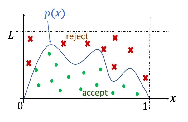
4 |
5 | ## Introduction
6 | This repository contains an implementation of the Monte Carlo Integration method in the F# programming language. The Monte Carlo method is a statistical technique used for estimating numerical results by simulating random sampling.
7 |
8 | ## Installation
9 | To run the provided code, ensure you have F# installed on your system. You can install F# using various methods depending on your operating system. Visit [F# Software Foundation](https://fsharp.org/use/) for installation instructions.
10 |
11 | ## Usage
12 | 1. Clone or download this repository to your local machine.
13 | 2. Navigate to the directory containing the code files.
14 | 3. Open a terminal or command prompt in that directory.
15 | 4. Execute the following command to compile and run the code:
16 |
17 | ```bash
18 | dotnet run
19 | ```
20 |
21 | ## Code explanation
22 |
23 | ```
24 | open System
25 |
26 | // Function to calculate the integral of a function using the Monte Carlo method
27 | let monteCarloIntegration (f: float -> float) (a: float) (b: float) (n: int) =
28 | let rand = System.Random()
29 | let mutable sum = 0.0
30 |
31 | for _ in 1 .. n do
32 | let x = a + (b - a) * rand.NextDouble()
33 | sum <- sum + f x
34 |
35 | let average = sum / float n
36 | let integral = average * (b - a)
37 | integral
38 |
39 |
40 | // Calculate the integral of sin(x) in the interval [0, π] using the Monte Carlo method
41 | let f x = sin x
42 | let a = 0.0
43 | let b = Math.PI
44 | let n = 1000000
45 |
46 | let integral = monteCarloIntegration f a b n
47 |
48 | printfn "The integral of sin(x) in the interval [0, π] using the Monte Carlo method is approximately %f" integral
49 | ```
50 |
51 | ## Example
52 |
53 | In this example, the code calculates the integral of the function $\sin(x)$ in the interval $[0, \pi]$ using the Monte Carlo method. The output provides an approximate value for the integral.
54 |
55 |
56 | ## References
57 |
58 | Ethan Smith. (2018, 30 junio). Monte Carlo Integration [Video]. YouTube. https://www.youtube.com/watch?v=8276ZswRw7M
--------------------------------------------------------------------------------
/src/Newton-Raphson-method/Newton-Raphson-method.fsproj:
--------------------------------------------------------------------------------
1 |
2 |
3 |
4 | Exe
5 | net7.0
6 | Newton_Raphson_method
7 |
8 |
9 |
10 |
11 |
12 |
13 |
14 |
--------------------------------------------------------------------------------
/src/Newton-Raphson-method/Program.fs:
--------------------------------------------------------------------------------
1 | open System
2 |
3 | let newtonRaphson (f: float -> float) (df: float -> float) (x0: float) (tol: float) (maxIter: int) =
4 | let rec loop (x: float) (iter: int) =
5 | let fx = f x
6 | let dfx = df x
7 | let x1 = x - fx / dfx
8 | if abs (x1 - x) < tol then x1
9 | elif iter < maxIter then loop x1 (iter + 1)
10 | else failwith "Newton-Raphson method failed to converge"
11 | loop x0 0
12 |
13 |
14 | let f x = x ** 3.0 - 2.0 * x - 5.0
15 | let df x = 3.0 * x ** 2.0 - 2.0
16 |
17 | let root = newtonRaphson f df 1.0 0.0001 1000
18 | printfn "The root of the function is %f" root
19 |
20 |
--------------------------------------------------------------------------------
/src/Newton-Raphson-method/README.md:
--------------------------------------------------------------------------------
1 | # Newton-Raphson method
2 |
3 | 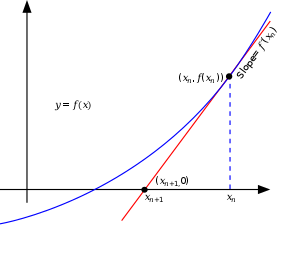
4 |
5 | ## Introduction
6 | This repository contains an implementation of the Newton-Raphson Method in F# programming language. The Newton-Raphson Method is a root-finding algorithm used to find successively better approximations to the roots (or zeroes) of a real-valued function. It is a powerful numerical technique commonly used for solving nonlinear equations.
7 |
8 | ## Installation
9 | To run the provided code, ensure you have F# installed on your system. You can install F# using various methods depending on your operating system. Visit [F# Software Foundation](https://fsharp.org/use/) for installation instructions.
10 |
11 | ## Usage
12 | 1. Clone or download this repository to your local machine.
13 | 2. Navigate to the directory containing the code files.
14 | 3. Open a terminal or command prompt in that directory.
15 | 4. Execute the following command to compile and run the code:
16 |
17 | ```bash
18 | dotnet run
19 | ```
20 |
21 | 5. The program will output the approximate root of the provided function.
22 |
23 | ## Code Explanation
24 | ```fsharp
25 | open System
26 |
27 | // Definition of the function implementing the Newton-Raphson method
28 | let newtonRaphson (f: float -> float) (df: float -> float) (x0: float) (tol: float) (maxIter: int) =
29 | // Definition of an inner function to iterate until convergence or reach the maximum number of iterations
30 | let rec loop (x: float) (iter: int) =
31 | let fx = f x // Compute the value of the function at x
32 | let dfx = df x // Compute the value of the derivative of the function at x
33 | let x1 = x - fx / dfx // Compute the next approximation of the root using the Newton-Raphson formula
34 | if abs (x1 - x) < tol then // Check if the difference between successive approximations is less than the tolerance
35 | x1 // Return the current approximation as the root if tolerance is satisfied
36 | elif iter < maxIter then // If tolerance is not met and the number of iterations is less than the maximum limit
37 | loop x1 (iter + 1) // Continue iterating with the new approximation
38 | else // If the maximum iteration limit is reached without convergence
39 | failwith "Newton-Raphson method failed to converge" // Raise an exception indicating failure to converge
40 |
41 | // Start the iteration process with the initial guess and iteration count set to 0
42 | loop x0 0
43 |
44 |
45 | let f x = x ** 3.0 - 2.0 * x - 5.0
46 | let df x = 3.0 * x ** 2.0 - 2.0
47 |
48 | // Call the Newton-Raphson method with the provided function, its derivative, initial guess, tolerance, and maximum iterations
49 | let root = newtonRaphson f df 1.0 0.0001 1000
50 |
51 | // Print the approximate root of the function
52 | printfn "The root of the function is %f" root
53 |
54 |
55 | ```
56 |
57 | ## Example
58 |
59 | For the provided function $f(x) = x^3 - 2x - 5$, the Newton-Raphson Method is used to approximate the root. In this example, the initial guess is $x_0 = 1.0$, with a tolerance of $0.0001$ and a maximum iteration limit of $1000$.
60 |
61 | ## References
62 |
63 | MathAndPhysics. (2020, 30 mayo). Newton-Raphson method | Animated and explained | Algorithm for finding roots of a function [Vídeo]. YouTube. https://www.youtube.com/watch?v=qlNqPE_X4ME
--------------------------------------------------------------------------------
/src/Numerical-differentiation/Numerical-differentiation.fsproj:
--------------------------------------------------------------------------------
1 |
2 |
3 |
4 | Exe
5 | net7.0
6 | Numerical_differentiation
7 |
8 |
9 |
10 |
11 |
12 |
13 |
14 |
--------------------------------------------------------------------------------
/src/Numerical-differentiation/Program.fs:
--------------------------------------------------------------------------------
1 | open System
2 |
3 | let diff (f: float -> float) (x: float) (h: float) =
4 | (f (x + h) - f (x - h)) / (2.0 * h)
5 |
6 | let f x = sin x
7 | let x = 0.0
8 | let h = 0.1
9 | let df = diff f x h
10 |
11 | printfn "The first derivative of sin(0) is approximately %f" df
12 |
13 |
14 |
--------------------------------------------------------------------------------
/src/Numerical-differentiation/README.md:
--------------------------------------------------------------------------------
1 | # Numerical differentiation
2 |
3 | 
4 |
5 | ## Introduction
6 | This repository contains an implementation of Numerical Differentiation in F# programming language. Numerical differentiation is a technique used to approximate the derivative of a function at a point using numerical methods, particularly when an analytical expression for the derivative is not available or is difficult to compute.
7 |
8 | ## Installation
9 | To run the provided code, ensure you have F# installed on your system. You can install F# using various methods depending on your operating system. Visit [F# Software Foundation](https://fsharp.org/use/) for installation instructions.
10 |
11 | ## Usage
12 | 1. Clone or download this repository to your local machine.
13 | 2. Navigate to the directory containing the code files.
14 | 3. Open a terminal or command prompt in that directory.
15 | 4. Execute the following command to compile and run the code:
16 |
17 | ```bash
18 | dotnet run
19 | ```
20 |
21 | 5. The program will output the approximate value of the derivative of the provided function at the specified point.
22 |
23 | ## Code Explanation
24 | ```fsharp
25 | open System
26 |
27 | // Define a function to compute the numerical differentiation of a given function at a point x with a step size h
28 | let diff (f: float -> float) (x: float) (h: float) =
29 | (f (x + h) - f (x - h)) / (2.0 * h)
30 |
31 | // Define the function for which we want to compute the derivative (e.g., sine function)
32 | let f x = sin x
33 |
34 | let x = 0.0 // Define the point at which to compute the derivative
35 | let h = 0.1 // Define the step size for numerical differentiation
36 |
37 | // Compute the numerical derivative of the function at point x with step size h
38 | let df = diff f x h
39 |
40 | // Print the approximate value of the derivative
41 | printfn "The first derivative of sin(0) is approximately %f" df
42 |
43 | ```
44 |
45 | ## Example
46 |
47 | In this example, the code computes the numerical differentiation of the sine function at point $x = 0$ using a step size of $h = 0.1$. The output provides an approximation of the first derivative of sine at $x = 0$.
48 |
49 | ## References
50 |
51 | StudySession. (2023b, julio 1). Introduction to numerical differentiation | Numerical Methods [Vídeo]. YouTube. https://www.youtube.com/watch?v=-3MwUJCDjts
--------------------------------------------------------------------------------
/src/Numerical-differentiation/obj/Numerical-differentiation.fsproj.nuget.dgspec.json:
--------------------------------------------------------------------------------
1 | {
2 | "format": 1,
3 | "restore": {
4 | "/home/jonas/Projects-NET/Numerical-methods-fs/src/Numerical-differentiation/Numerical-differentiation.fsproj": {}
5 | },
6 | "projects": {
7 | "/home/jonas/Projects-NET/Numerical-methods-fs/src/Numerical-differentiation/Numerical-differentiation.fsproj": {
8 | "version": "1.0.0",
9 | "restore": {
10 | "projectUniqueName": "/home/jonas/Projects-NET/Numerical-methods-fs/src/Numerical-differentiation/Numerical-differentiation.fsproj",
11 | "projectName": "Numerical-differentiation",
12 | "projectPath": "/home/jonas/Projects-NET/Numerical-methods-fs/src/Numerical-differentiation/Numerical-differentiation.fsproj",
13 | "packagesPath": "/home/jonas/.nuget/packages/",
14 | "outputPath": "/home/jonas/Projects-NET/Numerical-methods-fs/src/Numerical-differentiation/obj/",
15 | "projectStyle": "PackageReference",
16 | "configFilePaths": [
17 | "/home/jonas/.nuget/NuGet/NuGet.Config"
18 | ],
19 | "originalTargetFrameworks": [
20 | "net7.0"
21 | ],
22 | "sources": {
23 | "/usr/lib/dotnet/sdk/7.0.114/FSharp/library-packs": {},
24 | "https://api.nuget.org/v3/index.json": {}
25 | },
26 | "frameworks": {
27 | "net7.0": {
28 | "targetAlias": "net7.0",
29 | "projectReferences": {}
30 | }
31 | }
32 | },
33 | "frameworks": {
34 | "net7.0": {
35 | "targetAlias": "net7.0",
36 | "dependencies": {
37 | "FSharp.Core": {
38 | "include": "Runtime, Compile, Build, Native, Analyzers, BuildTransitive",
39 | "target": "Package",
40 | "version": "[7.0.0, )",
41 | "generatePathProperty": true
42 | }
43 | },
44 | "imports": [
45 | "net461",
46 | "net462",
47 | "net47",
48 | "net471",
49 | "net472",
50 | "net48",
51 | "net481"
52 | ],
53 | "assetTargetFallback": true,
54 | "warn": true,
55 | "frameworkReferences": {
56 | "Microsoft.NETCore.App": {
57 | "privateAssets": "all"
58 | }
59 | },
60 | "runtimeIdentifierGraphPath": "/usr/lib/dotnet/sdk/7.0.114/RuntimeIdentifierGraph.json"
61 | }
62 | }
63 | }
64 | }
65 | }
--------------------------------------------------------------------------------
/src/Numerical-differentiation/obj/Numerical-differentiation.fsproj.nuget.g.props:
--------------------------------------------------------------------------------
1 |
2 |
3 |
4 | True
5 | NuGet
6 | $(MSBuildThisFileDirectory)project.assets.json
7 | /home/jonas/.nuget/packages/
8 | /home/jonas/.nuget/packages/
9 | PackageReference
10 | 6.4.2
11 |
12 |
13 |
14 |
15 |
16 | /home/jonas/.nuget/packages/fsharp.core/7.0.0
17 |
18 |
--------------------------------------------------------------------------------
/src/Numerical-differentiation/obj/Numerical-differentiation.fsproj.nuget.g.targets:
--------------------------------------------------------------------------------
1 |
2 |
--------------------------------------------------------------------------------
/src/Numerical-differentiation/obj/project.assets.json:
--------------------------------------------------------------------------------
1 | {
2 | "version": 3,
3 | "targets": {
4 | "net7.0": {
5 | "FSharp.Core/7.0.0": {
6 | "type": "package",
7 | "compile": {
8 | "lib/netstandard2.1/FSharp.Core.dll": {
9 | "related": ".xml"
10 | }
11 | },
12 | "runtime": {
13 | "lib/netstandard2.1/FSharp.Core.dll": {
14 | "related": ".xml"
15 | }
16 | },
17 | "resource": {
18 | "lib/netstandard2.1/cs/FSharp.Core.resources.dll": {
19 | "locale": "cs"
20 | },
21 | "lib/netstandard2.1/de/FSharp.Core.resources.dll": {
22 | "locale": "de"
23 | },
24 | "lib/netstandard2.1/es/FSharp.Core.resources.dll": {
25 | "locale": "es"
26 | },
27 | "lib/netstandard2.1/fr/FSharp.Core.resources.dll": {
28 | "locale": "fr"
29 | },
30 | "lib/netstandard2.1/it/FSharp.Core.resources.dll": {
31 | "locale": "it"
32 | },
33 | "lib/netstandard2.1/ja/FSharp.Core.resources.dll": {
34 | "locale": "ja"
35 | },
36 | "lib/netstandard2.1/ko/FSharp.Core.resources.dll": {
37 | "locale": "ko"
38 | },
39 | "lib/netstandard2.1/pl/FSharp.Core.resources.dll": {
40 | "locale": "pl"
41 | },
42 | "lib/netstandard2.1/pt-BR/FSharp.Core.resources.dll": {
43 | "locale": "pt-BR"
44 | },
45 | "lib/netstandard2.1/ru/FSharp.Core.resources.dll": {
46 | "locale": "ru"
47 | },
48 | "lib/netstandard2.1/tr/FSharp.Core.resources.dll": {
49 | "locale": "tr"
50 | },
51 | "lib/netstandard2.1/zh-Hans/FSharp.Core.resources.dll": {
52 | "locale": "zh-Hans"
53 | },
54 | "lib/netstandard2.1/zh-Hant/FSharp.Core.resources.dll": {
55 | "locale": "zh-Hant"
56 | }
57 | }
58 | }
59 | }
60 | },
61 | "libraries": {
62 | "FSharp.Core/7.0.0": {
63 | "sha512": "vhHkNh35/K8FVNR/IJAKFxIahHh/00DQLRdiUdq2m+7zWHnR/A/uqs3sjF4OgCM4K7Naqpe2OgIiqeVxQgmCrg==",
64 | "type": "package",
65 | "path": "fsharp.core/7.0.0",
66 | "files": [
67 | ".nupkg.metadata",
68 | "Icon.png",
69 | "fsharp.core.7.0.0.nupkg.sha512",
70 | "fsharp.core.nuspec",
71 | "lib/netstandard2.0/FSharp.Core.dll",
72 | "lib/netstandard2.0/FSharp.Core.xml",
73 | "lib/netstandard2.0/cs/FSharp.Core.resources.dll",
74 | "lib/netstandard2.0/de/FSharp.Core.resources.dll",
75 | "lib/netstandard2.0/es/FSharp.Core.resources.dll",
76 | "lib/netstandard2.0/fr/FSharp.Core.resources.dll",
77 | "lib/netstandard2.0/it/FSharp.Core.resources.dll",
78 | "lib/netstandard2.0/ja/FSharp.Core.resources.dll",
79 | "lib/netstandard2.0/ko/FSharp.Core.resources.dll",
80 | "lib/netstandard2.0/pl/FSharp.Core.resources.dll",
81 | "lib/netstandard2.0/pt-BR/FSharp.Core.resources.dll",
82 | "lib/netstandard2.0/ru/FSharp.Core.resources.dll",
83 | "lib/netstandard2.0/tr/FSharp.Core.resources.dll",
84 | "lib/netstandard2.0/zh-Hans/FSharp.Core.resources.dll",
85 | "lib/netstandard2.0/zh-Hant/FSharp.Core.resources.dll",
86 | "lib/netstandard2.1/FSharp.Core.dll",
87 | "lib/netstandard2.1/FSharp.Core.xml",
88 | "lib/netstandard2.1/cs/FSharp.Core.resources.dll",
89 | "lib/netstandard2.1/de/FSharp.Core.resources.dll",
90 | "lib/netstandard2.1/es/FSharp.Core.resources.dll",
91 | "lib/netstandard2.1/fr/FSharp.Core.resources.dll",
92 | "lib/netstandard2.1/it/FSharp.Core.resources.dll",
93 | "lib/netstandard2.1/ja/FSharp.Core.resources.dll",
94 | "lib/netstandard2.1/ko/FSharp.Core.resources.dll",
95 | "lib/netstandard2.1/pl/FSharp.Core.resources.dll",
96 | "lib/netstandard2.1/pt-BR/FSharp.Core.resources.dll",
97 | "lib/netstandard2.1/ru/FSharp.Core.resources.dll",
98 | "lib/netstandard2.1/tr/FSharp.Core.resources.dll",
99 | "lib/netstandard2.1/zh-Hans/FSharp.Core.resources.dll",
100 | "lib/netstandard2.1/zh-Hant/FSharp.Core.resources.dll"
101 | ]
102 | }
103 | },
104 | "projectFileDependencyGroups": {
105 | "net7.0": [
106 | "FSharp.Core >= 7.0.0"
107 | ]
108 | },
109 | "packageFolders": {
110 | "/home/jonas/.nuget/packages/": {}
111 | },
112 | "project": {
113 | "version": "1.0.0",
114 | "restore": {
115 | "projectUniqueName": "/home/jonas/Projects-NET/Numerical-methods-fs/src/Numerical-differentiation/Numerical-differentiation.fsproj",
116 | "projectName": "Numerical-differentiation",
117 | "projectPath": "/home/jonas/Projects-NET/Numerical-methods-fs/src/Numerical-differentiation/Numerical-differentiation.fsproj",
118 | "packagesPath": "/home/jonas/.nuget/packages/",
119 | "outputPath": "/home/jonas/Projects-NET/Numerical-methods-fs/src/Numerical-differentiation/obj/",
120 | "projectStyle": "PackageReference",
121 | "configFilePaths": [
122 | "/home/jonas/.nuget/NuGet/NuGet.Config"
123 | ],
124 | "originalTargetFrameworks": [
125 | "net7.0"
126 | ],
127 | "sources": {
128 | "/usr/lib/dotnet/sdk/7.0.114/FSharp/library-packs": {},
129 | "https://api.nuget.org/v3/index.json": {}
130 | },
131 | "frameworks": {
132 | "net7.0": {
133 | "targetAlias": "net7.0",
134 | "projectReferences": {}
135 | }
136 | }
137 | },
138 | "frameworks": {
139 | "net7.0": {
140 | "targetAlias": "net7.0",
141 | "dependencies": {
142 | "FSharp.Core": {
143 | "include": "Runtime, Compile, Build, Native, Analyzers, BuildTransitive",
144 | "target": "Package",
145 | "version": "[7.0.0, )",
146 | "generatePathProperty": true
147 | }
148 | },
149 | "imports": [
150 | "net461",
151 | "net462",
152 | "net47",
153 | "net471",
154 | "net472",
155 | "net48",
156 | "net481"
157 | ],
158 | "assetTargetFallback": true,
159 | "warn": true,
160 | "frameworkReferences": {
161 | "Microsoft.NETCore.App": {
162 | "privateAssets": "all"
163 | }
164 | },
165 | "runtimeIdentifierGraphPath": "/usr/lib/dotnet/sdk/7.0.114/RuntimeIdentifierGraph.json"
166 | }
167 | }
168 | }
169 | }
--------------------------------------------------------------------------------
/src/Numerical-differentiation/obj/project.nuget.cache:
--------------------------------------------------------------------------------
1 | {
2 | "version": 2,
3 | "dgSpecHash": "Inlp+8TwaPZNrCimVHct84yEuGNlbT7I0BMUofL3Dy+7vsfOD1Rzh7pig/CiY/QFhDEyZd4d2pquduQneHv6Qg==",
4 | "success": true,
5 | "projectFilePath": "/home/jonas/Projects-NET/Numerical-methods-fs/src/Numerical-differentiation/Numerical-differentiation.fsproj",
6 | "expectedPackageFiles": [
7 | "/home/jonas/.nuget/packages/fsharp.core/7.0.0/fsharp.core.7.0.0.nupkg.sha512"
8 | ],
9 | "logs": []
10 | }
--------------------------------------------------------------------------------
/src/Numerical-integration-rectangle-rule/Numerical-integration-rectangle-rule.fsproj:
--------------------------------------------------------------------------------
1 |
2 |
3 |
4 | Exe
5 | net8.0
6 | Numerical_integration_rectangle_rule
7 |
8 |
9 |
10 |
11 |
12 |
13 |
14 |
--------------------------------------------------------------------------------
/src/Numerical-integration-rectangle-rule/Program.fs:
--------------------------------------------------------------------------------
1 | open System
2 |
3 | let rectangleRule (f: float -> float) (a: float) (b: float) (n: int) =
4 | let h = (b - a) / float n
5 | let sum =
6 | seq { for i in 0 .. n-1 -> a + float i * h }
7 | |> Seq.sumBy (fun xi -> f xi)
8 | h * sum
9 |
10 | let f x = sin x
11 | let a = 0.0
12 | let b = 1.0
13 | let n = 100
14 | let integral = rectangleRule f a b n
15 |
16 | printfn "The numerical integral of sin(x) from %f to %f using the rectangle rule is approximately %f" a b integral
--------------------------------------------------------------------------------
/src/Numerical-integration-rectangle-rule/README.md:
--------------------------------------------------------------------------------
1 | # Numerical Integration (Rectangle Rule) README
2 |
3 | 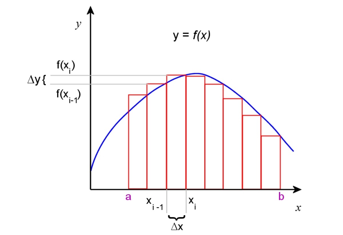
4 |
5 | ## Introduction
6 | This repository contains an implementation of Numerical Integration using the Rectangle Rule in the F# programming language. Numerical integration, also known as numerical quadrature, is a technique to approximate the definite integral of a function over a specified interval. The Rectangle Rule is a simple method where the area under the curve is approximated by dividing the interval into subintervals and using rectangles to approximate the area.
7 |
8 | ## Installation
9 | To run the provided code, ensure you have F# installed on your system. You can install F# using various methods depending on your operating system. Visit [F# Software Foundation](https://fsharp.org/use/) for installation instructions.
10 |
11 | ## Usage
12 | 1. Clone or download this repository to your local machine.
13 | 2. Navigate to the directory containing the code files.
14 | 3. Open a terminal or command prompt in that directory.
15 | 4. Execute the following command to compile and run the code:
16 |
17 | ```bash
18 | dotnet run
19 | ```
20 |
21 | 5. The program will output the approximate value of the integral of the provided function over the specified interval using the Rectangle Rule.
22 |
23 | ## Code Explanation
24 | ```fsharp
25 | open System
26 |
27 | // Define a function to compute numerical integration using the Rectangle Rule
28 | let rectangleRule (f: float -> float) (a: float) (b: float) (n: int) =
29 | let h = (b - a) / float n // Compute the width of each subinterval
30 | let sum =
31 | seq { for i in 0 .. n-1 -> a + float i * h } // Generate a sequence of x values within the interval
32 | |> Seq.sumBy (fun xi -> f xi) // Compute the sum of function values at each x value
33 | h * sum // Compute the approximate integral using the Rectangle Rule formula
34 |
35 | // Define the function for which we want to compute the integral (e.g., sine function)
36 | let f x = sin x
37 |
38 | let a = 0.0 // Define the lower limit of the interval
39 | let b = 1.0 // Define the upper limit of the interval
40 | let n = 100 // Define the number of subintervals
41 | let integral = rectangleRule f a b n // Compute the numerical integral using the Rectangle Rule
42 |
43 | // Print the approximate value of the integral
44 | printfn "The numerical integral of sin(x) from %f to %f using the Rectangle Rule is approximately %f" a b integral
45 | ```
46 |
47 | ## Example
48 | In this example, the code computes the numerical integral of the sine function from \( x = 0 \) to \( x = 1 \) using the Rectangle Rule with \( 100 \) subintervals. The output provides an approximation of the integral of sine over the specified interval.
49 |
50 | ## References
51 | Mrs O’Gram’s Maths. (2020, 21 abril). Integration: Numerical methods - Rectangle Rule [Vídeo]. YouTube. https://www.youtube.com/watch?v=TAbOyEyK0xE
--------------------------------------------------------------------------------
/src/Numerical-integration-simpson-rule/Numerical-integration-simpson-rule.fsproj:
--------------------------------------------------------------------------------
1 |
2 |
3 |
4 | Exe
5 | net8.0
6 | Numerical_integration_simpson_rule
7 |
8 |
9 |
10 |
11 |
12 |
13 |
14 |
--------------------------------------------------------------------------------
/src/Numerical-integration-simpson-rule/Program.fs:
--------------------------------------------------------------------------------
1 | open System
2 |
3 | let simpsonRule (f: float -> float) (a: float) (b: float) (n: int) =
4 | let h = (b - a) / float n
5 | let sum_odd =
6 | seq { for i in 1 .. n/2 -> a + 2.0 * float i * h }
7 | |> Seq.sumBy (fun xi -> f xi)
8 | let sum_even =
9 | seq { for i in 1 .. n/2-1 -> a + (2.0 * float i - 1.0) * h }
10 | |> Seq.sumBy (fun xi -> f xi)
11 | (h / 3.0) * (f a + 4.0 * sum_odd + 2.0 * sum_even + f b)
12 |
13 | let f x = sin x
14 | let a = 0.0
15 | let b = 1.0
16 | let n = 100
17 | let integral = simpsonRule f a b n
18 |
19 | printfn "The numerical integral of sin(x) from %f to %f using Simpson's rule is approximately %f" a b integral
20 |
--------------------------------------------------------------------------------
/src/Numerical-integration-simpson-rule/README.md:
--------------------------------------------------------------------------------
1 | # Numerical integration Simpson rule
2 |
3 | 
4 |
5 | ## Introduction
6 | This repository contains an implementation of Numerical Integration using Simpson's Rule in the F# programming language. Simpson's Rule is a numerical method used to approximate the definite integral of a function over a specified interval. It provides a more accurate approximation compared to methods like the Rectangle Rule or Trapezoidal Rule by using quadratic approximations of the function.
7 |
8 | ## Installation
9 | To run the provided code, ensure you have F# installed on your system. You can install F# using various methods depending on your operating system. Visit [F# Software Foundation](https://fsharp.org/use/) for installation instructions.
10 |
11 | ## Usage
12 | 1. Clone or download this repository to your local machine.
13 | 2. Navigate to the directory containing the code files.
14 | 3. Open a terminal or command prompt in that directory.
15 | 4. Execute the following command to compile and run the code:
16 |
17 | ```bash
18 | dotnet run
19 | ```
20 |
21 | 5. The program will output the approximate value of the integral of the provided function over the specified interval using Simpson's Rule.
22 |
23 | ## Code Explanation
24 | ```fsharp
25 | open System
26 |
27 | // Define a function to compute numerical integration using Simpson's Rule
28 | let simpsonRule (f: float -> float) (a: float) (b: float) (n: int) =
29 | let h = (b - a) / float n // Compute the width of each subinterval
30 | let sum_odd =
31 | seq { for i in 1 .. n/2 -> a + 2.0 * float i * h } // Generate a sequence of x values for odd indices
32 | |> Seq.sumBy (fun xi -> f xi) // Compute the sum of function values at odd indices
33 | let sum_even =
34 | seq { for i in 1 .. n/2-1 -> a + (2.0 * float i - 1.0) * h } // Generate a sequence of x values for even indices
35 | |> Seq.sumBy (fun xi -> f xi) // Compute the sum of function values at even indices
36 | (h / 3.0) * (f a + 4.0 * sum_odd + 2.0 * sum_even + f b) // Compute the approximate integral using Simpson's Rule formula
37 |
38 | // Define the function for which we want to compute the integral (e.g., sine function)
39 | let f x = sin x
40 |
41 | let a = 0.0 // Define the lower limit of the interval
42 | let b = 1.0 // Define the upper limit of the interval
43 | let n = 100 // Define the number of subintervals
44 | let integral = simpsonRule f a b n // Compute the numerical integral using Simpson's Rule
45 |
46 | // Print the approximate value of the integral
47 | printfn "The numerical integral of sin(x) from %f to %f using Simpson's Rule is approximately %f" a b integral
48 | ```
49 |
50 | ## Example
51 |
52 | In this example, the code computes the numerical integral of the sine function from $x = 0$ to $x = 1$ using Simpson's Rule with $100$ subintervals. The output provides an approximation of the integral of sine over the specified interval.
53 |
54 | ## References
55 |
56 | The Organic Chemistry Tutor. (2018, 13 marzo). Simpson’s Rule & Numerical Integration [Vídeo]. YouTube. https://www.youtube.com/watch?v=7EqRRuh-5Lk
57 |
--------------------------------------------------------------------------------
/src/Numerical-integration-trapezoidal-rule/Numerical-integration-trapezoidal-rule.fsproj:
--------------------------------------------------------------------------------
1 |
2 |
3 |
4 | Exe
5 | net8.0
6 | Numerical_integration_trapezoidal_rule
7 |
8 |
9 |
10 |
11 |
12 |
13 |
14 |
--------------------------------------------------------------------------------
/src/Numerical-integration-trapezoidal-rule/Program.fs:
--------------------------------------------------------------------------------
1 | open System
2 |
3 | let trapezoidalRule (f: float -> float) (a: float) (b: float) (n: int) =
4 | let h = (b - a) / float n
5 | let sum =
6 | seq { for i in 1 .. n-1 -> a + float i * h }
7 | |> Seq.sumBy (fun xi -> f xi)
8 | 0.5 * h * (f a + 2.0 * sum + f b)
9 |
10 | let f x = sin x
11 | let a = 0.0
12 | let b = 1.0
13 | let n = 100
14 | let integral = trapezoidalRule f a b n
15 |
16 | printfn "The numerical integral of sin(x) from %f to %f using trapezoidal rule is approximately %f" a b integral
17 |
--------------------------------------------------------------------------------
/src/Numerical-integration-trapezoidal-rule/README.md:
--------------------------------------------------------------------------------
1 | # Numerical integration trapezoidal rule
2 |
3 | 
4 |
5 | ## Introduction
6 | This repository contains an implementation of Numerical Integration using the Trapezoidal Rule in the F# programming language. The Trapezoidal Rule is a numerical method used to approximate the definite integral of a function over a specified interval. It provides a simple approximation by approximating the area under the curve with trapezoids.
7 |
8 | ## Installation
9 | To run the provided code, ensure you have F# installed on your system. You can install F# using various methods depending on your operating system. Visit [F# Software Foundation](https://fsharp.org/use/) for installation instructions.
10 |
11 | ## Usage
12 | 1. Clone or download this repository to your local machine.
13 | 2. Navigate to the directory containing the code files.
14 | 3. Open a terminal or command prompt in that directory.
15 | 4. Execute the following command to compile and run the code:
16 |
17 | ```bash
18 | dotnet run
19 | ```
20 |
21 | 5. The program will output the approximate value of the integral of the provided function over the specified interval using the Trapezoidal Rule.
22 |
23 | ## Code Explanation
24 | ```fsharp
25 | open System
26 |
27 | // Define a function to compute numerical integration using the Trapezoidal Rule
28 | let trapezoidalRule (f: float -> float) (a: float) (b: float) (n: int) =
29 | let h = (b - a) / float n // Compute the width of each subinterval
30 | let sum =
31 | seq { for i in 1 .. n-1 -> a + float i * h } // Generate a sequence of x values within the interval (excluding the endpoints)
32 | |> Seq.sumBy (fun xi -> f xi) // Compute the sum of function values at each x value
33 | 0.5 * h * (f a + 2.0 * sum + f b) // Compute the approximate integral using the Trapezoidal Rule formula
34 |
35 | // Define the function for which we want to compute the integral (e.g., sine function)
36 | let f x = sin x
37 |
38 | let a = 0.0 // Define the lower limit of the interval
39 | let b = 1.0 // Define the upper limit of the interval
40 | let n = 100 // Define the number of subintervals
41 | let integral = trapezoidalRule f a b n // Compute the numerical integral using the Trapezoidal Rule
42 |
43 | // Print the approximate value of the integral
44 | printfn "The numerical integral of sin(x) from %f to %f using the Trapezoidal Rule is approximately %f" a b integral
45 | ```
46 |
47 | ## Example
48 |
49 | In this example, the code computes the numerical integral of the sine function from \(x = 0\) to \(x = 1\) using the Trapezoidal Rule with \(100\) subintervals. The output provides an approximation of the integral of sine over the specified interval.
50 |
51 | ## References
52 |
53 | The Organic Chemistry Tutor. (2018b, marzo 13). Trapezoidal rule [Vídeo]. YouTube. https://www.youtube.com/watch?v=Rn9Gr52zhrY
54 |
--------------------------------------------------------------------------------
/src/Runge-kutta-method/Program.fs:
--------------------------------------------------------------------------------
1 | open System
2 |
3 | // Function for solving an ordinary differential equation (EDO) using the fourth-order Runge–Kutta method
4 |
5 | let rungeKutta4Method (f: float -> float -> float) (x0: float) (y0: float) (xf: float) (h: float) =
6 | let mutable x = x0
7 | let mutable y = y0
8 | let mutable values = []
9 |
10 | while x <= xf do
11 | values <- (x, y) :: values
12 | let k1 = h * f x y
13 | let k2 = h * f (x + h / 2.0) (y + k1 / 2.0)
14 | let k3 = h * f (x + h / 2.0) (y + k2 / 2.0)
15 | let k4 = h * f (x + h) (y + k3)
16 | y <- y + (k1 + 2.0 * k2 + 2.0 * k3 + k4) / 6.0
17 | x <- x + h
18 |
19 | values |> List.rev
20 |
21 | // Example: Solve the ordinary differential equation (EDO) y' = -2y, y(0) = 1, for x in [0, 2] with step size h = 0.1
22 |
23 | let f x y = -2.0 * y
24 | let x0 = 0.0
25 | let y0 = 1.0
26 | let xf = 2.0
27 | let h = 0.1
28 |
29 | let solution = rungeKutta4Method f x0 y0 xf h
30 | printfn "Solution:"
31 | solution |> List.iter (fun (x, y) -> printfn "x = %f, y = %f" x y)
32 |
33 |
--------------------------------------------------------------------------------
/src/Runge-kutta-method/README.md:
--------------------------------------------------------------------------------
1 | # Runge kutta method
2 |
3 | 
4 |
5 | ## Introduction
6 | This repository contains an implementation of the fourth-order Runge-Kutta method in the F# programming language. The Runge-Kutta method is a numerical technique used to solve ordinary differential equations (ODEs) numerically. It is a popular method known for its accuracy and stability.
7 |
8 | ## Implementation
9 | The provided code demonstrates the use of the fourth-order Runge-Kutta method to solve an ordinary differential equation (ODE) of the form y' = -2y, with the initial condition y(0) = 1, over the interval [0, 2] with a step size of h = 0.1.
10 |
11 | ## Usage
12 | 1. Clone or download this repository to your local machine.
13 | 2. Navigate to the directory containing the code files.
14 | 3. Open a terminal or command prompt in that directory.
15 | 4. Execute the following command to compile and run the code:
16 |
17 | ```bash
18 | dotnet run
19 | ```
20 |
21 | 5. The program will output the solution points (x, y) along the solution curve.
22 |
23 | ## Code Explanation
24 |
25 | ```fsharp
26 | // Function for solving an ordinary differential equation (ODE) using the fourth-order Runge–Kutta method
27 | let rungeKutta4Method (f: float -> float -> float) (x0: float) (y0: float) (xf: float) (h: float) =
28 | let mutable x = x0 // Initialize x with the initial value
29 | let mutable y = y0 // Initialize y with the initial value
30 | let mutable values = [] // Initialize an empty list to store solution points
31 |
32 | while x <= xf do // Loop until x reaches the final value xf
33 | values <- (x, y) :: values // Append the current solution point to the list
34 | let k1 = h * f x y // Calculate the first slope component
35 | let k2 = h * f (x + h / 2.0) (y + k1 / 2.0) // Calculate the second slope component
36 | let k3 = h * f (x + h / 2.0) (y + k2 / 2.0) // Calculate the third slope component
37 | let k4 = h * f (x + h) (y + k3) // Calculate the fourth slope component
38 | y <- y + (k1 + 2.0 * k2 + 2.0 * k3 + k4) / 6.0 // Update y using the weighted average of slopes
39 | x <- x + h // Increment x by the step size
40 |
41 | values |> List.rev // Reverse the list of solution points (optional)
42 |
43 |
44 | // Example: Solve the ordinary differential equation (EDO) y' = -2y, y(0) = 1, for x in [0, 2] with step size h = 0.1
45 |
46 | let f x y = -2.0 * y
47 | let x0 = 0.0
48 | let y0 = 1.0
49 | let xf = 2.0
50 | let h = 0.1
51 |
52 | let solution = rungeKutta4Method f x0 y0 xf h
53 | printfn "Solution:"
54 | solution |> List.iter (fun (x, y) -> printfn "x = %f, y = %f" x y)
55 | ```
56 |
57 | ## Example
58 | In this example, the code solves the ODE y' = -2y with the initial condition y(0) = 1, for x in the interval [0, 2] with a step size h = 0.1 using the fourth-order Runge-Kutta method. The output provides the solution points (x, y) along the solution curve.
59 |
60 | ## References
61 |
62 | Jeffrey Chasnov. (2021c, febrero 10). Runge Kutta Methods | Lecture 50 | Numerical Methods for Engineers [Video]. YouTube. https://www.youtube.com/watch?v=C4UymmEi3Kw
--------------------------------------------------------------------------------
/src/Runge-kutta-method/Runge-kutta-method.fsproj:
--------------------------------------------------------------------------------
1 |
2 |
3 |
4 | Exe
5 | net8.0
6 | Runge_kutta_method
7 |
8 |
9 |
10 |
11 |
12 |
13 |
14 |
--------------------------------------------------------------------------------