├── MIMO
├── assets
│ ├── RxMRC.png
│ ├── TxMRC.png
│ ├── Tarokh.png
│ ├── fadings.png
│ ├── mu-mimo.jpg
│ ├── outage.png
│ ├── svd-mimo.png
│ ├── Alamouti_1.jpg
│ ├── Alamouti_2.jpg
│ ├── Alamouti_4.png
│ ├── BERRician1.png
│ ├── BERRician2.png
│ ├── MIMO-OFDM.png
│ ├── MIMOscheme.png
│ ├── array-fig.png
│ ├── capacity-1.jpg
│ ├── capacity-2.jpg
│ ├── diversity.png
│ ├── fad-source.png
│ ├── test-model.png
│ ├── AlamoutiForm.png
│ ├── Alamouti_06.png
│ ├── MIMObasics_r.png
│ ├── mimo-tensor.png
│ ├── mu-mimo-techs.png
│ ├── parall-siso.png
│ ├── rice-rayleigh.png
│ ├── Coherence time.png
│ ├── Correlated_case.png
│ ├── Kroneker Model.jpg
│ ├── mu-mimo-scheme.png
│ ├── MIMObasics_3d_ed.png
│ ├── Rician_SISO_MIMO.jpg
│ ├── Uncorrelated_case.png
│ ├── pre-code-post-proc.png
│ ├── Coherence bandwidth.png
│ ├── fading-transmission.png
│ └── rice-rayleigh-SCHEME.png
├── Rician_flat_channel.m
├── Alamouti_Rician.m
├── MIMO Capacity.py
├── Spatial_Correlation.ipynb
├── Alamouti.ipynb
└── RicianFlatFadingMATLAB.ipynb
├── LICENSE
└── README.md
/MIMO/assets/RxMRC.png:
--------------------------------------------------------------------------------
https://raw.githubusercontent.com/kirlf/CSP/HEAD/MIMO/assets/RxMRC.png
--------------------------------------------------------------------------------
/MIMO/assets/TxMRC.png:
--------------------------------------------------------------------------------
https://raw.githubusercontent.com/kirlf/CSP/HEAD/MIMO/assets/TxMRC.png
--------------------------------------------------------------------------------
/MIMO/assets/Tarokh.png:
--------------------------------------------------------------------------------
https://raw.githubusercontent.com/kirlf/CSP/HEAD/MIMO/assets/Tarokh.png
--------------------------------------------------------------------------------
/MIMO/assets/fadings.png:
--------------------------------------------------------------------------------
https://raw.githubusercontent.com/kirlf/CSP/HEAD/MIMO/assets/fadings.png
--------------------------------------------------------------------------------
/MIMO/assets/mu-mimo.jpg:
--------------------------------------------------------------------------------
https://raw.githubusercontent.com/kirlf/CSP/HEAD/MIMO/assets/mu-mimo.jpg
--------------------------------------------------------------------------------
/MIMO/assets/outage.png:
--------------------------------------------------------------------------------
https://raw.githubusercontent.com/kirlf/CSP/HEAD/MIMO/assets/outage.png
--------------------------------------------------------------------------------
/MIMO/assets/svd-mimo.png:
--------------------------------------------------------------------------------
https://raw.githubusercontent.com/kirlf/CSP/HEAD/MIMO/assets/svd-mimo.png
--------------------------------------------------------------------------------
/MIMO/assets/Alamouti_1.jpg:
--------------------------------------------------------------------------------
https://raw.githubusercontent.com/kirlf/CSP/HEAD/MIMO/assets/Alamouti_1.jpg
--------------------------------------------------------------------------------
/MIMO/assets/Alamouti_2.jpg:
--------------------------------------------------------------------------------
https://raw.githubusercontent.com/kirlf/CSP/HEAD/MIMO/assets/Alamouti_2.jpg
--------------------------------------------------------------------------------
/MIMO/assets/Alamouti_4.png:
--------------------------------------------------------------------------------
https://raw.githubusercontent.com/kirlf/CSP/HEAD/MIMO/assets/Alamouti_4.png
--------------------------------------------------------------------------------
/MIMO/assets/BERRician1.png:
--------------------------------------------------------------------------------
https://raw.githubusercontent.com/kirlf/CSP/HEAD/MIMO/assets/BERRician1.png
--------------------------------------------------------------------------------
/MIMO/assets/BERRician2.png:
--------------------------------------------------------------------------------
https://raw.githubusercontent.com/kirlf/CSP/HEAD/MIMO/assets/BERRician2.png
--------------------------------------------------------------------------------
/MIMO/assets/MIMO-OFDM.png:
--------------------------------------------------------------------------------
https://raw.githubusercontent.com/kirlf/CSP/HEAD/MIMO/assets/MIMO-OFDM.png
--------------------------------------------------------------------------------
/MIMO/assets/MIMOscheme.png:
--------------------------------------------------------------------------------
https://raw.githubusercontent.com/kirlf/CSP/HEAD/MIMO/assets/MIMOscheme.png
--------------------------------------------------------------------------------
/MIMO/assets/array-fig.png:
--------------------------------------------------------------------------------
https://raw.githubusercontent.com/kirlf/CSP/HEAD/MIMO/assets/array-fig.png
--------------------------------------------------------------------------------
/MIMO/assets/capacity-1.jpg:
--------------------------------------------------------------------------------
https://raw.githubusercontent.com/kirlf/CSP/HEAD/MIMO/assets/capacity-1.jpg
--------------------------------------------------------------------------------
/MIMO/assets/capacity-2.jpg:
--------------------------------------------------------------------------------
https://raw.githubusercontent.com/kirlf/CSP/HEAD/MIMO/assets/capacity-2.jpg
--------------------------------------------------------------------------------
/MIMO/assets/diversity.png:
--------------------------------------------------------------------------------
https://raw.githubusercontent.com/kirlf/CSP/HEAD/MIMO/assets/diversity.png
--------------------------------------------------------------------------------
/MIMO/assets/fad-source.png:
--------------------------------------------------------------------------------
https://raw.githubusercontent.com/kirlf/CSP/HEAD/MIMO/assets/fad-source.png
--------------------------------------------------------------------------------
/MIMO/assets/test-model.png:
--------------------------------------------------------------------------------
https://raw.githubusercontent.com/kirlf/CSP/HEAD/MIMO/assets/test-model.png
--------------------------------------------------------------------------------
/MIMO/assets/AlamoutiForm.png:
--------------------------------------------------------------------------------
https://raw.githubusercontent.com/kirlf/CSP/HEAD/MIMO/assets/AlamoutiForm.png
--------------------------------------------------------------------------------
/MIMO/assets/Alamouti_06.png:
--------------------------------------------------------------------------------
https://raw.githubusercontent.com/kirlf/CSP/HEAD/MIMO/assets/Alamouti_06.png
--------------------------------------------------------------------------------
/MIMO/assets/MIMObasics_r.png:
--------------------------------------------------------------------------------
https://raw.githubusercontent.com/kirlf/CSP/HEAD/MIMO/assets/MIMObasics_r.png
--------------------------------------------------------------------------------
/MIMO/assets/mimo-tensor.png:
--------------------------------------------------------------------------------
https://raw.githubusercontent.com/kirlf/CSP/HEAD/MIMO/assets/mimo-tensor.png
--------------------------------------------------------------------------------
/MIMO/assets/mu-mimo-techs.png:
--------------------------------------------------------------------------------
https://raw.githubusercontent.com/kirlf/CSP/HEAD/MIMO/assets/mu-mimo-techs.png
--------------------------------------------------------------------------------
/MIMO/assets/parall-siso.png:
--------------------------------------------------------------------------------
https://raw.githubusercontent.com/kirlf/CSP/HEAD/MIMO/assets/parall-siso.png
--------------------------------------------------------------------------------
/MIMO/assets/rice-rayleigh.png:
--------------------------------------------------------------------------------
https://raw.githubusercontent.com/kirlf/CSP/HEAD/MIMO/assets/rice-rayleigh.png
--------------------------------------------------------------------------------
/MIMO/assets/Coherence time.png:
--------------------------------------------------------------------------------
https://raw.githubusercontent.com/kirlf/CSP/HEAD/MIMO/assets/Coherence time.png
--------------------------------------------------------------------------------
/MIMO/assets/Correlated_case.png:
--------------------------------------------------------------------------------
https://raw.githubusercontent.com/kirlf/CSP/HEAD/MIMO/assets/Correlated_case.png
--------------------------------------------------------------------------------
/MIMO/assets/Kroneker Model.jpg:
--------------------------------------------------------------------------------
https://raw.githubusercontent.com/kirlf/CSP/HEAD/MIMO/assets/Kroneker Model.jpg
--------------------------------------------------------------------------------
/MIMO/assets/mu-mimo-scheme.png:
--------------------------------------------------------------------------------
https://raw.githubusercontent.com/kirlf/CSP/HEAD/MIMO/assets/mu-mimo-scheme.png
--------------------------------------------------------------------------------
/MIMO/assets/MIMObasics_3d_ed.png:
--------------------------------------------------------------------------------
https://raw.githubusercontent.com/kirlf/CSP/HEAD/MIMO/assets/MIMObasics_3d_ed.png
--------------------------------------------------------------------------------
/MIMO/assets/Rician_SISO_MIMO.jpg:
--------------------------------------------------------------------------------
https://raw.githubusercontent.com/kirlf/CSP/HEAD/MIMO/assets/Rician_SISO_MIMO.jpg
--------------------------------------------------------------------------------
/MIMO/assets/Uncorrelated_case.png:
--------------------------------------------------------------------------------
https://raw.githubusercontent.com/kirlf/CSP/HEAD/MIMO/assets/Uncorrelated_case.png
--------------------------------------------------------------------------------
/MIMO/assets/pre-code-post-proc.png:
--------------------------------------------------------------------------------
https://raw.githubusercontent.com/kirlf/CSP/HEAD/MIMO/assets/pre-code-post-proc.png
--------------------------------------------------------------------------------
/MIMO/assets/Coherence bandwidth.png:
--------------------------------------------------------------------------------
https://raw.githubusercontent.com/kirlf/CSP/HEAD/MIMO/assets/Coherence bandwidth.png
--------------------------------------------------------------------------------
/MIMO/assets/fading-transmission.png:
--------------------------------------------------------------------------------
https://raw.githubusercontent.com/kirlf/CSP/HEAD/MIMO/assets/fading-transmission.png
--------------------------------------------------------------------------------
/MIMO/assets/rice-rayleigh-SCHEME.png:
--------------------------------------------------------------------------------
https://raw.githubusercontent.com/kirlf/CSP/HEAD/MIMO/assets/rice-rayleigh-SCHEME.png
--------------------------------------------------------------------------------
/LICENSE:
--------------------------------------------------------------------------------
1 | MIT License
2 |
3 | Copyright (c) 2019 Vladimir Fadeev
4 |
5 | Permission is hereby granted, free of charge, to any person obtaining a copy
6 | of this software and associated documentation files (the "Software"), to deal
7 | in the Software without restriction, including without limitation the rights
8 | to use, copy, modify, merge, publish, distribute, sublicense, and/or sell
9 | copies of the Software, and to permit persons to whom the Software is
10 | furnished to do so, subject to the following conditions:
11 |
12 | The above copyright notice and this permission notice shall be included in all
13 | copies or substantial portions of the Software.
14 |
15 | THE SOFTWARE IS PROVIDED "AS IS", WITHOUT WARRANTY OF ANY KIND, EXPRESS OR
16 | IMPLIED, INCLUDING BUT NOT LIMITED TO THE WARRANTIES OF MERCHANTABILITY,
17 | FITNESS FOR A PARTICULAR PURPOSE AND NONINFRINGEMENT. IN NO EVENT SHALL THE
18 | AUTHORS OR COPYRIGHT HOLDERS BE LIABLE FOR ANY CLAIM, DAMAGES OR OTHER
19 | LIABILITY, WHETHER IN AN ACTION OF CONTRACT, TORT OR OTHERWISE, ARISING FROM,
20 | OUT OF OR IN CONNECTION WITH THE SOFTWARE OR THE USE OR OTHER DEALINGS IN THE
21 | SOFTWARE.
22 |
--------------------------------------------------------------------------------
/MIMO/Rician_flat_channel.m:
--------------------------------------------------------------------------------
1 | clear all; close all; clc
2 |
3 | EbNo = 0:40;
4 | K = [4.0; 0.6];
5 | M = [4; 8; 16; 64; 256]; %Positions of modulation (M-PSK or M-QAM)
6 |
7 | for k = 1:length(K)
8 | for m = 1:length(M)
9 | message = randi([0, M(m)-1], 100000, 1);
10 | if M(m) >= 16
11 | mod_msg = qammod(message, M(m), pi/4, 'gray');
12 | ric_ber(:, m, k) = berfading(EbNo,'qam',M(m),1,K(k));
13 | else
14 | mod_msg = pskmod(message, M(m), pi/4, 'gray');
15 | ric_ber(:, m, k) = berfading(EbNo, 'psk', M(m), 1, K(k));
16 | end
17 | Es = mean(abs(mod_msg).^2);
18 | No = Es./((10.^(EbNo./10))*log2(M(m)));
19 |
20 | h = sqrt( K(k)/(K(k)+1)) +...
21 | sqrt( 1/(K(k)+1))*(1/sqrt(2))*(randn(size(mod_msg))...
22 | + 1j*randn(size(mod_msg)));
23 | ric_msg = mod_msg.*h; % Rician flat fading
24 |
25 | for c = 1:100
26 | for jj = 1:length(EbNo)
27 | noisy_mod = ric_msg +...
28 | sqrt(No(jj)/2)*(randn(size(mod_msg))+...
29 | 1j*randn(size(mod_msg))); %AWGN
30 | noisy_mod = noisy_mod ./ h; % zero-forcing equalization
31 | if M(m) >= 16
32 | demod_msg = qamdemod(noisy_mod, M(m), pi/4, 'gray');
33 | else
34 | demod_msg = pskdemod(noisy_mod, M(m), pi/4, 'gray');
35 | end
36 | [number,BER(c,jj)] = biterr(message,demod_msg);
37 | end
38 | end
39 | sum_BER(:,m, k) = sum(BER)./c;
40 | end
41 | end
42 |
43 | figure(1)
44 |
45 | semilogy(EbNo, sum_BER(:,1,1), 'b-o', EbNo, sum_BER(:,2,1), 'r-o',...
46 | EbNo, sum_BER(:,3,1), 'g-o', EbNo, sum_BER(:,4,1), 'c-o',...
47 | EbNo, sum_BER(:,5,1), 'k-o',...
48 | EbNo, ric_ber(:,1,1), 'b-', EbNo, ric_ber(:,2,1), 'r-',...
49 | EbNo, ric_ber(:,3,1), 'g-', EbNo, ric_ber(:,4,1), 'c-',...
50 | EbNo, ric_ber(:,5,1), 'k-', 'LineWidth', 1.5)
51 | title('Rician model (K = 4.0)')
52 | legend('QPSK(simulated)', '8-PSK(simulated)',...
53 | '16-QAM(simulated)', '64-QAM(simulated)' ,'256-QAM(simulated)',...
54 | 'QPSK(theory)','8-PSK(theory)', '16-QAM(theory)',...
55 | '64-QAM(theory)' ,'256-QAM(theory)','location','best')
56 | xlabel('EbNo (dB)')
57 | ylabel('BER')
58 | grid on
59 |
60 |
61 | figure(2)
62 |
63 | semilogy(EbNo, sum_BER(:,1,2), 'b-o', EbNo, sum_BER(:,2,2), 'r-o',...
64 | EbNo, sum_BER(:,3,2), 'g-o', EbNo, sum_BER(:,4,2), 'c-o',...
65 | EbNo, sum_BER(:,5,2), 'k-o',...
66 | EbNo, ric_ber(:,1,2), 'b-', EbNo, ric_ber(:,2,2), 'r-',...
67 | EbNo, ric_ber(:,3,2), 'g-', EbNo,ric_ber(:,4,2), 'c-',...
68 | EbNo, ric_ber(:,5,2), 'k-','LineWidth', 1.5)
69 | title('Rician model (K = 0.6)')
70 | legend('QPSK(simulated)', '8-PSK(simulated)',...
71 | '16-QAM(simulated)', '64-QAM(simulated)' ,'256-QAM(simulated)',...
72 | 'QPSK(theory)','8-PSK(theory)',...
73 | '16-QAM(theory)', '64-QAM(theory)' ,'256-QAM(theory)','location','best')
74 | xlabel('EbNo (dB)')
75 | ylabel('BER')
76 | grid on
--------------------------------------------------------------------------------
/MIMO/Alamouti_Rician.m:
--------------------------------------------------------------------------------
1 | clear all; close all; clc
2 |
3 | snapshots = 100000;
4 | EbNo = 0:10;
5 | K = [4.0; 0.6];
6 | M = [4; 8]; %Positions of modulation (M-PSK)
7 | Mt = 2;
8 | Mr = [1; 2];
9 |
10 | ostbcEnc = comm.OSTBCEncoder('NumTransmitAntennas', Mt); % Alamouti
11 |
12 | ric_ber = zeros(length(EbNo), length(M), length(K), length(Mr));
13 | sum_BER = zeros(length(EbNo), length(M), length(K), length(Mr));
14 |
15 |
16 | for mr = 1:length(Mr)
17 | ostbcComb = comm.OSTBCCombiner('NumTransmitAntennas', Mt, 'NumReceiveAntennas', Mr(mr));
18 | H = zeros(Mr(mr), Mt, snapshots);
19 | ric_msg = zeros(snapshots, Mr(mr));
20 | for k = 1:length(K)
21 | mu = sqrt( K(k)/(K(k)+1));
22 | s = sqrt(1/(K(k)+1));
23 | for m = 1:length(M)
24 |
25 | hModulator = comm.PSKModulator('ModulationOrder', M(m), 'BitInput', false);
26 | hDemod = comm.PSKDemodulator('ModulationOrder', M(m), 'BitOutput', false);
27 | ric_ber(:,m,k,mr) = berfading(EbNo, 'psk', M(m), Mr(mr)*Mt, K(k));
28 |
29 | snr = EbNo+10*log10(log2(M(m)));
30 | message = randi([0,M(m)-1],100000,1);
31 |
32 | mod_msg = step(hModulator,message);
33 | Es = mean(abs(mod_msg).^2);
34 |
35 | alam_msg = step(ostbcEnc, mod_msg);
36 |
37 | % Channel
38 | h = mu + s*(1/sqrt(2))*(randn(Mr(mr),Mt,snapshots/Mt)...
39 | + 1j*randn(Mr(mr),Mt, snapshots/Mt));
40 | H(:,:,1:2:end-1) = h;
41 | H(:,:,2:2:end) = h;
42 | pathGainself = permute(H,[3,2,1]);
43 |
44 | % Transmit through the channel
45 | for q = 1:snapshots;
46 | ric_msg(q,:) = (sqrt(Es/Mt)*H(:,:,q)*alam_msg(q,:).').';
47 | end
48 |
49 | for c = 1:100
50 | for jj = 1:length(EbNo)
51 | noisy_mod = awgn(ric_msg,snr(jj),'measured','dB');
52 | decodeData = step(ostbcComb,noisy_mod,pathGainself);
53 | demod_msg = step(hDemod,decodeData);
54 | [number,BER(c,jj)] = biterr(message,demod_msg);
55 | end
56 | end
57 | sum_BER(:,m, k, mr) = sum(BER)./c;
58 | end
59 | end
60 | end
61 |
62 | figure(1)
63 |
64 | semilogy(EbNo,sum_BER(:,1,1,1),'r-o',EbNo,sum_BER(:,2,1,1),'g-o',...
65 | EbNo,ric_ber(:,1,1,1),'r-',EbNo,ric_ber(:,2,1,1),'g-',...
66 | EbNo,sum_BER(:,1,1,2),'b-o',EbNo,sum_BER(:,2,1,2),'y-o',...
67 | EbNo,ric_ber(:,1,1,2),'b-',EbNo,ric_ber(:,2,1,2),'y-',...
68 | 'LineWidth', 1.5)
69 | title('Rician model (K = 4.0)')
70 | legend('QPSK(simulated) 2x1', '8-PSK(simulated) 2x1',...
71 | 'QPSK(theory) 2x1','8-PSK(theory) 2x1',...
72 | 'QPSK(simulated) 2x2', '8-PSK(simulated) 2x2',...
73 | 'QPSK(theory) 2x2','8-PSK(theory) 2x2')
74 | xlabel('EbNo (dB)')
75 | ylabel('BER')
76 | grid on
77 |
78 |
79 | figure(2)
80 |
81 | semilogy(EbNo,sum_BER(:,1,2,1),'r-o',EbNo,sum_BER(:,2,2,1),'g-o',...
82 | EbNo,ric_ber(:,1,2,1),'r-',EbNo,ric_ber(:,2,2,1),'g-',...
83 | EbNo,sum_BER(:,1,2,2),'b-o',EbNo,sum_BER(:,2,2,2),'y-o',...
84 | EbNo,ric_ber(:,1,2,2),'b-',EbNo,ric_ber(:,2,2,2),'y-',...
85 | 'LineWidth', 1.5)
86 | title('Rician model (K = 0.6)')
87 | legend('QPSK(simulated) 2x1', '8-PSK(simulated) 2x1',...
88 | 'QPSK(theory) 2x1','8-PSK(theory) 2x1',...
89 | 'QPSK(simulated) 2x2', '8-PSK(simulated) 2x2',...
90 | 'QPSK(theory) 2x2','8-PSK(theory) 2x2')
91 | xlabel('EbNo (dB)')
92 | ylabel('BER')
93 | grid on
--------------------------------------------------------------------------------
/MIMO/MIMO Capacity.py:
--------------------------------------------------------------------------------
1 | #!/usr/bin/env python
2 | # coding: utf-8
3 |
4 | # # MIMO Channel Capacity
5 | # ### M.Sc. Vladimir Fadeev
6 | # #### Kazan, 2018
7 |
8 |
9 | import numpy as np
10 | from numpy import linalg as LA
11 | import warnings
12 | warnings.filterwarnings('ignore')
13 | import matplotlib.pyplot as plt
14 |
15 |
16 | def waterpouring(Mt, SNR_dB, H_chan):
17 | SNR = 10**(SNR_dB/10)
18 | r = LA.matrix_rank(H_chan)
19 | H_sq = np.dot(H_chan,np.matrix(H_chan, dtype=complex).H)
20 | lambdas = LA.eigvals(H_sq)
21 | lambdas = np.sort(lambdas)[::-1]
22 | p = 1;
23 | gammas = np.zeros((r,1))
24 | flag = True
25 | while flag == True:
26 | lambdas_r_p_1 = lambdas[0:(r-p+1)]
27 | inv_lambdas_sum = np.sum(1/lambdas_r_p_1)
28 | mu = ( Mt / (r - p + 1) ) * ( 1 + (1/SNR) * inv_lambdas_sum)
29 | for idx, item in enumerate(lambdas_r_p_1):
30 | gammas[idx] = mu - (Mt/(SNR*item))
31 | if gammas[r-p] < 0: #due to Python starts from 0
32 | gammas[r-p] = 0 #due to Python starts from 0
33 | p = p + 1
34 | else:
35 | flag = False
36 | res = []
37 | for gamma in gammas:
38 | res.append(float(gamma))
39 | return np.array(res)
40 |
41 | #Test
42 | Mt = 3
43 | SNR_db = 10
44 | H_chan = np.array([[1,0,2],[0,1,0], [0,1,0]], dtype = float)
45 | gammas = waterpouring(Mt, SNR_db, H_chan)
46 | print('Rank of the matrix: '+str(LA.matrix_rank(H_chan)))
47 | print('Gammas:\n'+str(gammas))
48 |
49 |
50 | # Short comparison
51 |
52 |
53 | def openloop_capacity(H_chan, SNR_dB):
54 | SNR = 10**(SNR_dB/10)
55 | Mt = np.shape(H_chan)[1]
56 | H_sq = np.dot(H_chan,np.matrix(H_chan, dtype=complex).H)
57 | lambdas = LA.eigvals(H_sq)
58 | lambdas = np.sort(lambdas)[::-1]
59 | c = 0
60 | for eig in lambdas:
61 | c = c + np.log2(1 + SNR*eig/Mt)
62 | return np.real(c)
63 |
64 | Mr = 4
65 | Mt = 4
66 | H_chan = (np.random.randn(Mr,Mt) + 1j*np.random.randn(Mr, Mt))/np.sqrt(2) #Rayleigh flat fading
67 | c = openloop_capacity(H_chan, 10)
68 | print(c)
69 |
70 |
71 | def closedloop_capacity(H_chan, SNR_dB):
72 | SNR = 10**(SNR_dB/10)
73 | Mt = np.shape(H_chan)[1]
74 | H_sq = np.dot(H_chan,np.matrix(H_chan, dtype=complex).H)
75 | lambdas = LA.eigvals(H_sq)
76 | lambdas = np.real(np.sort(lambdas))[::-1]
77 | c = 0
78 | gammas = waterpouring(Mt, SNR_dB, H_chan)
79 | for idx, item in enumerate(lambdas):
80 | c = c + np.log2(1+ SNR*item*gammas[idx]/Mt)
81 | return np.real(c)
82 |
83 | c = closedloop_capacity(H_chan, 10)
84 | print(c)
85 |
86 |
87 |
88 | Mr = 4
89 | Mt = 4
90 | counter = 1000
91 | SNR_dBs = [i for i in range(1, 21)]
92 | C_open = np.empty((len(SNR_dBs), counter))
93 | C_closed = np.empty((len(SNR_dBs), counter))
94 |
95 | for c in range(counter):
96 | H_chan = (np.random.randn(Mr,Mt) + 1j*np.random.randn(Mr, Mt))/np.sqrt(2)
97 | for idx, SNR_dB in enumerate(SNR_dBs):
98 | C_open[idx, c] = openloop_capacity(H_chan, SNR_dB)
99 | C_closed[idx, c] = closedloop_capacity(H_chan, SNR_dB)
100 |
101 | C_open_erg = np.mean(C_open, axis=1)
102 | C_closed_erg = np.mean(C_closed, axis=1)
103 |
104 |
105 | fig = plt.figure(figsize=(10, 5), dpi=300)
106 | plt.plot(SNR_dBs, C_open_erg, label='Channel Unknown (CU)')
107 | plt.plot(SNR_dBs, C_closed_erg, label='Channel Known (CK)')
108 | plt.title("Ergodic Capacity")
109 | plt.xlabel('SNR (dB)')
110 | plt.ylabel('Capacity (bps/Hz)')
111 | plt.legend()
112 | plt.grid()
113 | plt.show()
114 |
115 |
116 | # # Reference
117 | #
118 | # 1. Paulraj, Arogyaswami, Rohit Nabar, and Dhananjay Gore.
119 | # Introduction to space-time wireless communications. Cambridge university press, 2003.
120 |
121 | # # Suggested literature
122 | #
123 | # 1. Haykin S. Communication systems. – John Wiley & Sons, 2008. - p.366-368
124 |
--------------------------------------------------------------------------------
/README.md:
--------------------------------------------------------------------------------
1 | # Communication and Signal Processing: MIMO
2 | ### M.Sc. Vladimir Fadeev
3 |
4 | **Additional teaching materials for the [Communication and Signal Processing (CSP)](https://griat.kai.ru/communications-and-signal-processing) major of German-Russian Institute of Advanced Technologies (GRIAT): Multiple Input Multiple Output (MIMO) technology.**
5 |
6 | 
7 |
8 | ## Summary
9 |
10 | - Desirable background:
11 | * [Rician flat fading (SISO)](https://nbviewer.jupyter.org/github/kirlf/CSP/blob/master/MIMO/RicianFlatFadingMATLAB.ipynb)
12 | - Tutorials:
13 | * [MIMO channel capacity](https://nbviewer.jupyter.org/github/kirlf/CSP/blob/master/MIMO/MIMO%20Capacity.ipynb)
14 | * [Space-Time Codes (Alamouti)](https://nbviewer.jupyter.org/github/kirlf/CSP/blob/master/MIMO/Alamouti.ipynb)
15 | - Self-education:
16 | * [Spatial correlation (tasks)](https://nbviewer.jupyter.org/github/kirlf/CSP/blob/master/MIMO/Spatial_Correlation.ipynb)
17 |
18 |
19 | ## Preface
20 |
21 | This work is prepared for students of **MS-CSP** (**C**ommunication and **S**ignal **P**rocessing) program (GRIAT) primarily. However, everyone who is interested in considered topics is welcome!
22 |
23 | ## Motivation
24 |
25 | Why should you learn MIMO technology basics?
26 |
27 | MIMO is a part of the most of modern wireless communication standards. For example, this is implemented in **LTE/LTE-A** networks and in Wi-Fi devices since **802.11n** (Wi-Fi 4).
28 |
29 | Moreover, the evolution of the MIMO - Massive MIMO is a part of the **5G** networks. This fact means scientific interest, and science is impossible without basics.
30 |
31 | 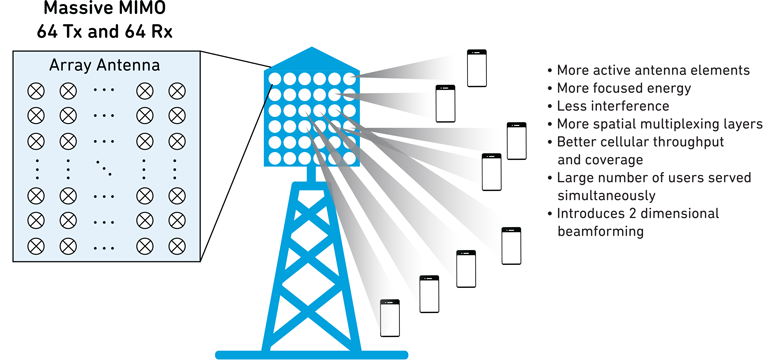 32 |
33 | > [Realizing 5G Sub-6-GHz Massive MIMO Using GaN](https://www.mwrf.com/semiconductors/realizing-5g-sub-6-ghz-massive-mimo-using-gan)
34 |
35 | Additionally, MIMO topic is a good opportunity to train your **linear algebra** skills!
36 |
37 | ## Suggested literature
38 |
39 | * Paulraj, Arogyaswami, Rohit Nabar, and Dhananjay Gore. Introduction to space-time wireless communications. Cambridge university press, 2003.
40 | * Salehi, M., and J. Proakis. "Digital communications." McGraw-Hill Education 31 (2007): 32.
41 | * Haykin, Simon S. Digital communications. New York: Wiley, 1988.
42 | * Goldsmith, Andrea. [Wireless communications.](http://wsl.stanford.edu/~andrea/Wireless/Book.pdf) Cambridge university press, 2005.
43 | * Sklar, Bernard. Digital communications: fundamentals and applications. 2001.
44 |
45 | ## See also
46 |
47 | The work on this project inspired me to write several popular science articles in my native language. Probably, it can be also helpful for someone:
48 |
49 | * [Оцениваем пропускную способность MIMO канала (алгоритм Water-pouring прилагается)](https://habr.com/ru/post/448570/)
50 | * [MU-MIMO: один из алгоритмов реализации](https://habr.com/ru/post/450948/)
51 | * [MIMO spatial diversity: Аламоути, DET и прочее пространственное разнесение](https://habr.com/ru/post/452494/)
52 | * [Почти самый простой MIMO канал с замираниями (модель Кронекера прилагается)](https://habr.com/ru/post/447172/)
53 |
54 | And several matherials about adaptive and array signal processing:
55 | * [Adaptive beamforming](https://gist.github.com/kirlf/afa2ac6fc0acb93edb7984c9bb1d6e63) (Python 3 source code)
56 | * [Adaptive filters](https://gist.github.com/kirlf/8e77cc17b7b1be4e35dbf651ff82f759) (Python 3 / MATLAB source codes)
57 | * [Моделируем алгоритм MUSIC для задач определения направления прихода электромагнитной волны](https://habr.com/ru/post/446674/)
58 | * [Оптимальная линейная фильтрация: от метода градиентного спуска до адаптивных фильтров](https://habr.com/ru/post/455497/)
59 |
60 | ## Comments and feedback
61 |
62 | I'll be appreciate your **stars** because in my oppinion this is one of the brightest indicators of a good work!
63 |
64 | You also can send your comments and suggestion by e-mail: vovenur@gmail.com
65 |
66 | The feedback is valuable for me!
67 |
68 | Have a nice reading, good day, and good luck!
69 |
70 | M.Sc. Vladimir Fadeev
71 |
--------------------------------------------------------------------------------
/MIMO/Spatial_Correlation.ipynb:
--------------------------------------------------------------------------------
1 | {
2 | "cells": [
3 | {
4 | "cell_type": "markdown",
5 | "metadata": {},
6 | "source": [
7 | "# Spatial Correlation (tasks)\n",
8 | "## M.Sc. Vladimir Fadeev\n",
9 | "### Kazan, 15.03.2019"
10 | ]
11 | },
12 | {
13 | "cell_type": "markdown",
14 | "metadata": {},
15 | "source": [
16 | "# Theory\n",
17 | "\n",
18 | "Ideally, spatial channels should be independent to each other, i.e. uncorrelated. \n",
19 | "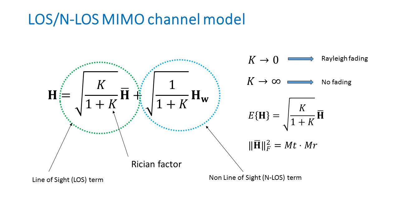\n",
20 | "\n",
21 | "However, it is almost unreachable case in real systems. Therefore we can calculate spatial correlation matrix to estimate correlation:\n",
22 | "\n",
23 | "$$ \\mathbf{R} = E\\left\\{vec\\left(H\\right)\\left(vec\\left(H\\right)\\right)^H\\right\\} \\qquad (1) $$\n",
24 | "\n",
25 | "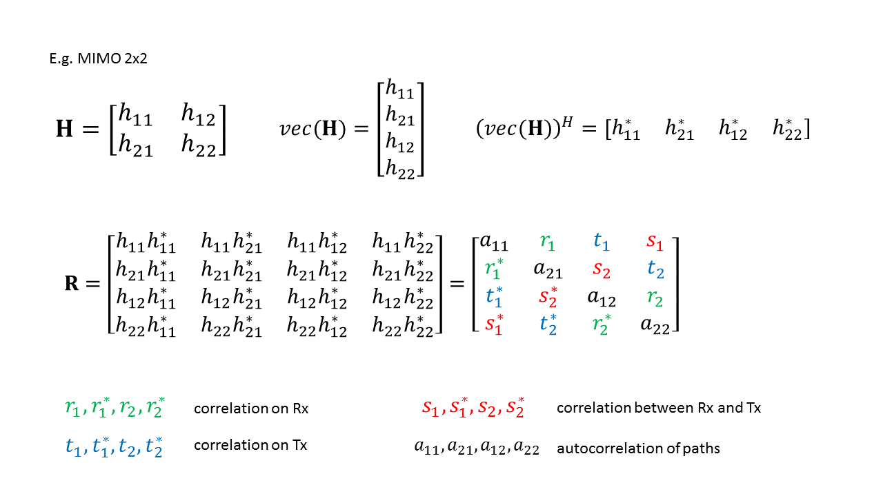"
26 | ]
27 | },
28 | {
29 | "cell_type": "markdown",
30 | "metadata": {},
31 | "source": [
32 | "If the Tx and Rx sides are **uncorrelated** (e.g. fig. 1) to each other, simplification can be applied: **Kronecker model**. \n",
33 | "\n",
34 | "\n",
35 | "\n",
36 | "*Fig. 1. The scatters model in case of uncorrelated Rx and Tx. Green dots mean scatters, blue and red - RX and Tx.*\n",
37 | "\n",
38 | "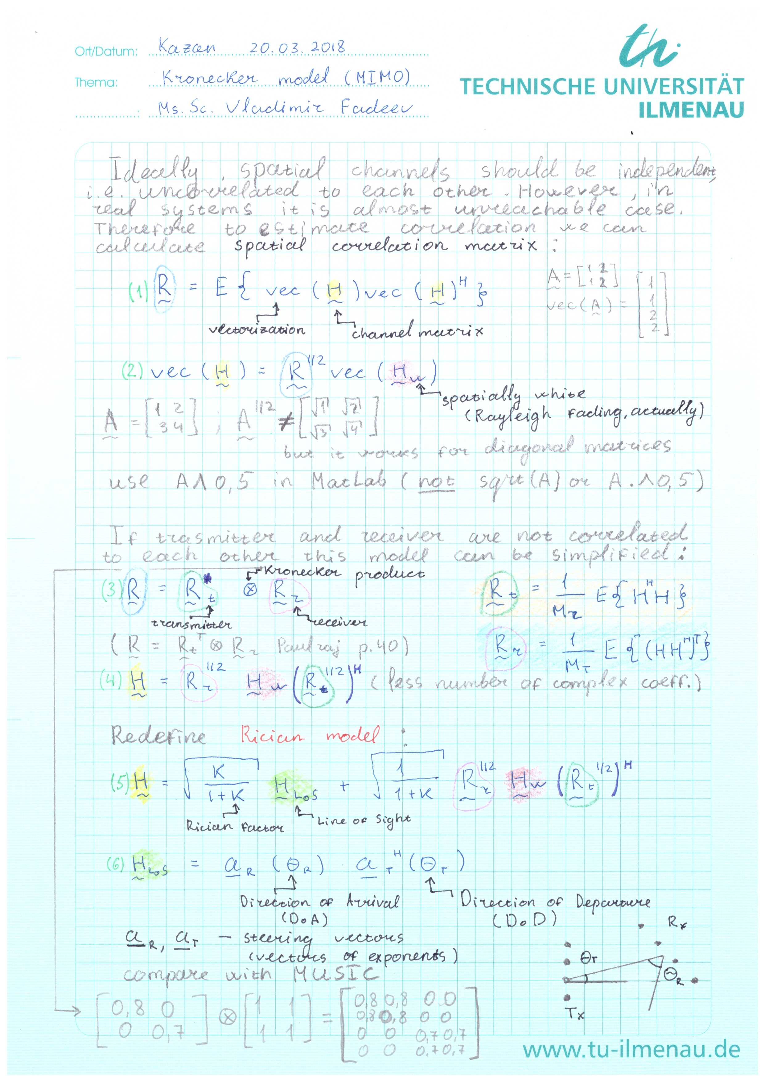"
39 | ]
40 | },
41 | {
42 | "cell_type": "markdown",
43 | "metadata": {},
44 | "source": [
45 | "However, in case of correlated channel (e.g. fig. 2) the formula (1) should be used.\n",
46 | "\n",
47 | "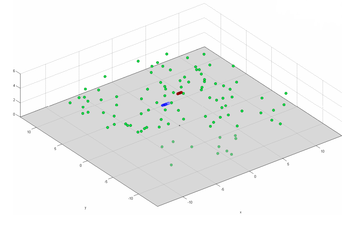 \n",
48 | "\n",
49 | "*Fig. 2. The scatters model in case of correlated Rx and Tx. Green dots mean scatters, blue and red - RX and Tx.*"
50 | ]
51 | },
52 | {
53 | "cell_type": "markdown",
54 | "metadata": {},
55 | "source": [
56 | "# Tasks"
57 | ]
58 | },
59 | {
60 | "cell_type": "markdown",
61 | "metadata": {},
62 | "source": [
63 | "## Task #1\n",
64 | "\n",
65 | "If we consider the Kroneker model, can we say that $r_1 = r_2$ and $t_1 = t_2$?\n",
66 | "\n",
67 | "What about $3\\times 3$ or $4 \\times 3$ channels?\n",
68 | "\n",
69 | "**Hint**: See \\[1, p.40\\] about the Kronecker product and properties of $\\mathbf{R}_T$ and $\\mathbf{R}_R$.\n",
70 | "\n",
71 | "\n",
72 | "\n",
73 | "## Task #2\n",
74 | "\n",
75 | "Calculate all of the $\\gamma^{opt}$ if $\\mathbf{R}_T = \\begin{bmatrix} 0.6 & 0 \\\\ 0 & 0.7 \\end{bmatrix}$ and $\\mathbf{R}_R = \\begin{bmatrix} 1 && 1 \\\\ 1 && 1 \\end{bmatrix}$, if SNR $-> + \\infty$ (values of co-variance matrices are random, the main part is the logic of the solution).\n",
76 | "\n",
77 | "**Hint**: Use the Water-pouring algorithm and see \\[1, p.40\\].\n",
78 | "\n",
79 | "## Task #3\n",
80 | "\n",
81 | "Is it possible to use Kronecker model for the following case:\n",
82 | "$$\\mathbf{R} = \\begin{bmatrix} 1 && 0.6 && 0.4 && 0.9 \\\\ 0.6 && 1 && 0.8 && 0.4 \\\\ 0.4 && 0.8 && 1 && 0.6 \\\\ 0.9 && 0.4 && 0.6 && 1 \\end{bmatrix}$$\n",
83 | "\n",
84 | "Explain why, if not. If yes, explain too.\n"
85 | ]
86 | },
87 | {
88 | "cell_type": "markdown",
89 | "metadata": {},
90 | "source": [
91 | "# Reference"
92 | ]
93 | },
94 | {
95 | "cell_type": "markdown",
96 | "metadata": {},
97 | "source": [
98 | "1. Paulraj, Arogyaswami, Rohit Nabar, and Dhananjay Gore. Introduction to space-time wireless communications. Cambridge university press, 2003."
99 | ]
100 | }
101 | ],
102 | "metadata": {
103 | "kernelspec": {
104 | "display_name": "Python 3",
105 | "language": "python",
106 | "name": "python3"
107 | },
108 | "language_info": {
109 | "codemirror_mode": {
110 | "name": "ipython",
111 | "version": 3
112 | },
113 | "file_extension": ".py",
114 | "mimetype": "text/x-python",
115 | "name": "python",
116 | "nbconvert_exporter": "python",
117 | "pygments_lexer": "ipython3",
118 | "version": "3.6.4"
119 | }
120 | },
121 | "nbformat": 4,
122 | "nbformat_minor": 2
123 | }
124 |
--------------------------------------------------------------------------------
/MIMO/Alamouti.ipynb:
--------------------------------------------------------------------------------
1 | {
2 | "cells": [
3 | {
4 | "cell_type": "markdown",
5 | "metadata": {},
6 | "source": [
7 | "# Space-Time codes (Alamouti)\n",
8 | "## (MATLAB tutorial)\n",
9 | "### M.Sc. Vladimir Fadeev\n",
10 | "#### Kazan, 04.02.2019"
11 | ]
12 | },
13 | {
14 | "cell_type": "markdown",
15 | "metadata": {},
16 | "source": [
17 | "# Introduction"
18 | ]
19 | },
20 | {
21 | "cell_type": "markdown",
22 | "metadata": {},
23 | "source": [
24 | "There are a lot of problems of the radiowave transmission in the mobile communication networks. For example, attenuations, reflections, refractions, scatterings, frequency Doppler shifts etc. You can find some of the aspects of this topic in the [following tutorial](https://github.com/kirlf/CSP/blob/master/Channels/RicianFlatFading.ipynb). All of the multiplicative random distortions can be collected under the **fading** term.\n",
25 | "\n",
26 | "Different techniques exist for the fading supression, let us count some of them:\n",
27 | "\n",
28 | "1. [Frequency hopping](http://www.teletopix.org/gsm/slow-and-fast-frequency-hopping-in-gsm/) (to suppress frequency selectivity);\n",
29 | "2. Channel estimation and equalization via feedbacks (GSM, to suppress time variability);\n",
30 | "3. [Spectrum spreading](https://www.tu-ilmenau.de/fileadmin/public/iks/files/lehre/UMTS/09_WCDMA_ws18_19.pdf) (UMTS);\n",
31 | "4. Pilots (since UMTS) in Down-link and signal tracking in Up-link (to suppress time variability);\n",
32 | "5. [OFDM](https://www.tu-ilmenau.de/fileadmin/public/iks/files/lehre/UMTS/11_LTE_Radio_ws18.pdf) (LTE, to suppress frequency selectivity);\n",
33 | "6. [Time diversity (channel coding)](https://github.com/kirlf/CSP/tree/master/FEC);\n",
34 | "7. Polarization diversity (transmitter side) + Combiners (receiver side);\n",
35 | "8. **Space diversity** (see below).\n",
36 | "\n",
37 | "\n",
38 | "\n",
39 | "\n"
40 | ]
41 | },
42 | {
43 | "cell_type": "markdown",
44 | "metadata": {},
45 | "source": [
46 | "# Space diversity and array gain"
47 | ]
48 | },
49 | {
50 | "cell_type": "markdown",
51 | "metadata": {},
52 | "source": [
53 | "Applying the MISO, SIMO or MIMO techniques (in other words, using more antennas) we can achieve increasing of the **devirsity order**: the same information can be collected from the different directions (pathes) and, hence, with lower probability to be corrupted. Theoretical limit of the diversity order is the $M_TM_R$, where $M_T$ is the number of the transmit antennas, and $M_R$ is the number of the receive antennas.\n",
54 | "\n",
55 | "
32 |
33 | > [Realizing 5G Sub-6-GHz Massive MIMO Using GaN](https://www.mwrf.com/semiconductors/realizing-5g-sub-6-ghz-massive-mimo-using-gan)
34 |
35 | Additionally, MIMO topic is a good opportunity to train your **linear algebra** skills!
36 |
37 | ## Suggested literature
38 |
39 | * Paulraj, Arogyaswami, Rohit Nabar, and Dhananjay Gore. Introduction to space-time wireless communications. Cambridge university press, 2003.
40 | * Salehi, M., and J. Proakis. "Digital communications." McGraw-Hill Education 31 (2007): 32.
41 | * Haykin, Simon S. Digital communications. New York: Wiley, 1988.
42 | * Goldsmith, Andrea. [Wireless communications.](http://wsl.stanford.edu/~andrea/Wireless/Book.pdf) Cambridge university press, 2005.
43 | * Sklar, Bernard. Digital communications: fundamentals and applications. 2001.
44 |
45 | ## See also
46 |
47 | The work on this project inspired me to write several popular science articles in my native language. Probably, it can be also helpful for someone:
48 |
49 | * [Оцениваем пропускную способность MIMO канала (алгоритм Water-pouring прилагается)](https://habr.com/ru/post/448570/)
50 | * [MU-MIMO: один из алгоритмов реализации](https://habr.com/ru/post/450948/)
51 | * [MIMO spatial diversity: Аламоути, DET и прочее пространственное разнесение](https://habr.com/ru/post/452494/)
52 | * [Почти самый простой MIMO канал с замираниями (модель Кронекера прилагается)](https://habr.com/ru/post/447172/)
53 |
54 | And several matherials about adaptive and array signal processing:
55 | * [Adaptive beamforming](https://gist.github.com/kirlf/afa2ac6fc0acb93edb7984c9bb1d6e63) (Python 3 source code)
56 | * [Adaptive filters](https://gist.github.com/kirlf/8e77cc17b7b1be4e35dbf651ff82f759) (Python 3 / MATLAB source codes)
57 | * [Моделируем алгоритм MUSIC для задач определения направления прихода электромагнитной волны](https://habr.com/ru/post/446674/)
58 | * [Оптимальная линейная фильтрация: от метода градиентного спуска до адаптивных фильтров](https://habr.com/ru/post/455497/)
59 |
60 | ## Comments and feedback
61 |
62 | I'll be appreciate your **stars** because in my oppinion this is one of the brightest indicators of a good work!
63 |
64 | You also can send your comments and suggestion by e-mail: vovenur@gmail.com
65 |
66 | The feedback is valuable for me!
67 |
68 | Have a nice reading, good day, and good luck!
69 |
70 | M.Sc. Vladimir Fadeev
71 |
--------------------------------------------------------------------------------
/MIMO/Spatial_Correlation.ipynb:
--------------------------------------------------------------------------------
1 | {
2 | "cells": [
3 | {
4 | "cell_type": "markdown",
5 | "metadata": {},
6 | "source": [
7 | "# Spatial Correlation (tasks)\n",
8 | "## M.Sc. Vladimir Fadeev\n",
9 | "### Kazan, 15.03.2019"
10 | ]
11 | },
12 | {
13 | "cell_type": "markdown",
14 | "metadata": {},
15 | "source": [
16 | "# Theory\n",
17 | "\n",
18 | "Ideally, spatial channels should be independent to each other, i.e. uncorrelated. \n",
19 | "\n",
20 | "\n",
21 | "However, it is almost unreachable case in real systems. Therefore we can calculate spatial correlation matrix to estimate correlation:\n",
22 | "\n",
23 | "$$ \\mathbf{R} = E\\left\\{vec\\left(H\\right)\\left(vec\\left(H\\right)\\right)^H\\right\\} \\qquad (1) $$\n",
24 | "\n",
25 | ""
26 | ]
27 | },
28 | {
29 | "cell_type": "markdown",
30 | "metadata": {},
31 | "source": [
32 | "If the Tx and Rx sides are **uncorrelated** (e.g. fig. 1) to each other, simplification can be applied: **Kronecker model**. \n",
33 | "\n",
34 | "\n",
35 | "\n",
36 | "*Fig. 1. The scatters model in case of uncorrelated Rx and Tx. Green dots mean scatters, blue and red - RX and Tx.*\n",
37 | "\n",
38 | ""
39 | ]
40 | },
41 | {
42 | "cell_type": "markdown",
43 | "metadata": {},
44 | "source": [
45 | "However, in case of correlated channel (e.g. fig. 2) the formula (1) should be used.\n",
46 | "\n",
47 | " \n",
48 | "\n",
49 | "*Fig. 2. The scatters model in case of correlated Rx and Tx. Green dots mean scatters, blue and red - RX and Tx.*"
50 | ]
51 | },
52 | {
53 | "cell_type": "markdown",
54 | "metadata": {},
55 | "source": [
56 | "# Tasks"
57 | ]
58 | },
59 | {
60 | "cell_type": "markdown",
61 | "metadata": {},
62 | "source": [
63 | "## Task #1\n",
64 | "\n",
65 | "If we consider the Kroneker model, can we say that $r_1 = r_2$ and $t_1 = t_2$?\n",
66 | "\n",
67 | "What about $3\\times 3$ or $4 \\times 3$ channels?\n",
68 | "\n",
69 | "**Hint**: See \\[1, p.40\\] about the Kronecker product and properties of $\\mathbf{R}_T$ and $\\mathbf{R}_R$.\n",
70 | "\n",
71 | "\n",
72 | "\n",
73 | "## Task #2\n",
74 | "\n",
75 | "Calculate all of the $\\gamma^{opt}$ if $\\mathbf{R}_T = \\begin{bmatrix} 0.6 & 0 \\\\ 0 & 0.7 \\end{bmatrix}$ and $\\mathbf{R}_R = \\begin{bmatrix} 1 && 1 \\\\ 1 && 1 \\end{bmatrix}$, if SNR $-> + \\infty$ (values of co-variance matrices are random, the main part is the logic of the solution).\n",
76 | "\n",
77 | "**Hint**: Use the Water-pouring algorithm and see \\[1, p.40\\].\n",
78 | "\n",
79 | "## Task #3\n",
80 | "\n",
81 | "Is it possible to use Kronecker model for the following case:\n",
82 | "$$\\mathbf{R} = \\begin{bmatrix} 1 && 0.6 && 0.4 && 0.9 \\\\ 0.6 && 1 && 0.8 && 0.4 \\\\ 0.4 && 0.8 && 1 && 0.6 \\\\ 0.9 && 0.4 && 0.6 && 1 \\end{bmatrix}$$\n",
83 | "\n",
84 | "Explain why, if not. If yes, explain too.\n"
85 | ]
86 | },
87 | {
88 | "cell_type": "markdown",
89 | "metadata": {},
90 | "source": [
91 | "# Reference"
92 | ]
93 | },
94 | {
95 | "cell_type": "markdown",
96 | "metadata": {},
97 | "source": [
98 | "1. Paulraj, Arogyaswami, Rohit Nabar, and Dhananjay Gore. Introduction to space-time wireless communications. Cambridge university press, 2003."
99 | ]
100 | }
101 | ],
102 | "metadata": {
103 | "kernelspec": {
104 | "display_name": "Python 3",
105 | "language": "python",
106 | "name": "python3"
107 | },
108 | "language_info": {
109 | "codemirror_mode": {
110 | "name": "ipython",
111 | "version": 3
112 | },
113 | "file_extension": ".py",
114 | "mimetype": "text/x-python",
115 | "name": "python",
116 | "nbconvert_exporter": "python",
117 | "pygments_lexer": "ipython3",
118 | "version": "3.6.4"
119 | }
120 | },
121 | "nbformat": 4,
122 | "nbformat_minor": 2
123 | }
124 |
--------------------------------------------------------------------------------
/MIMO/Alamouti.ipynb:
--------------------------------------------------------------------------------
1 | {
2 | "cells": [
3 | {
4 | "cell_type": "markdown",
5 | "metadata": {},
6 | "source": [
7 | "# Space-Time codes (Alamouti)\n",
8 | "## (MATLAB tutorial)\n",
9 | "### M.Sc. Vladimir Fadeev\n",
10 | "#### Kazan, 04.02.2019"
11 | ]
12 | },
13 | {
14 | "cell_type": "markdown",
15 | "metadata": {},
16 | "source": [
17 | "# Introduction"
18 | ]
19 | },
20 | {
21 | "cell_type": "markdown",
22 | "metadata": {},
23 | "source": [
24 | "There are a lot of problems of the radiowave transmission in the mobile communication networks. For example, attenuations, reflections, refractions, scatterings, frequency Doppler shifts etc. You can find some of the aspects of this topic in the [following tutorial](https://github.com/kirlf/CSP/blob/master/Channels/RicianFlatFading.ipynb). All of the multiplicative random distortions can be collected under the **fading** term.\n",
25 | "\n",
26 | "Different techniques exist for the fading supression, let us count some of them:\n",
27 | "\n",
28 | "1. [Frequency hopping](http://www.teletopix.org/gsm/slow-and-fast-frequency-hopping-in-gsm/) (to suppress frequency selectivity);\n",
29 | "2. Channel estimation and equalization via feedbacks (GSM, to suppress time variability);\n",
30 | "3. [Spectrum spreading](https://www.tu-ilmenau.de/fileadmin/public/iks/files/lehre/UMTS/09_WCDMA_ws18_19.pdf) (UMTS);\n",
31 | "4. Pilots (since UMTS) in Down-link and signal tracking in Up-link (to suppress time variability);\n",
32 | "5. [OFDM](https://www.tu-ilmenau.de/fileadmin/public/iks/files/lehre/UMTS/11_LTE_Radio_ws18.pdf) (LTE, to suppress frequency selectivity);\n",
33 | "6. [Time diversity (channel coding)](https://github.com/kirlf/CSP/tree/master/FEC);\n",
34 | "7. Polarization diversity (transmitter side) + Combiners (receiver side);\n",
35 | "8. **Space diversity** (see below).\n",
36 | "\n",
37 | "\n",
38 | "\n",
39 | "\n"
40 | ]
41 | },
42 | {
43 | "cell_type": "markdown",
44 | "metadata": {},
45 | "source": [
46 | "# Space diversity and array gain"
47 | ]
48 | },
49 | {
50 | "cell_type": "markdown",
51 | "metadata": {},
52 | "source": [
53 | "Applying the MISO, SIMO or MIMO techniques (in other words, using more antennas) we can achieve increasing of the **devirsity order**: the same information can be collected from the different directions (pathes) and, hence, with lower probability to be corrupted. Theoretical limit of the diversity order is the $M_TM_R$, where $M_T$ is the number of the transmit antennas, and $M_R$ is the number of the receive antennas.\n",
54 | "\n",
55 | " \n",
56 | "\n",
57 | "> *Fig.1. Link stability induced with increasing orders of spatial diversity. In the limit, as $M_TM_R \\to \\infty$, the channel is perfectly stabilized and approaches an AWGN link \\[1, p.101\\]*.\n",
58 | "\n",
59 | "> **NOTE**:\n",
60 | "> Considered trerm means also that we sacrifice the data rate (compared to spatial multiplexing schemes) to achieve better quality. \n",
61 | "\n",
62 | "Moreover, using SIMO, MIMO or MISO (in case of the known channel) techniques **array gain** can be achieved. This means that application of the several receive antennas allows to increase the Signal-to-Noise ratio (SNR) on the receiver side. Theoretical limit of the array gain is the $M_R$.\n",
63 | "\n",
64 | "Diversity orders and array gains of the differnt configurations can be summarized in the tabel 1. for both channel is unknown (CU) and channel is known (CK) on the transmitter side.\n",
65 | "\n",
66 | ">Table. 1. Array gain and diversity order for \n",
67 | ">different multiple antenna configurations\n",
68 | "\n",
69 | "| Configuration | Diversity order | Array gain |\n",
70 | "| ------------- |:-------------:| -----:|\n",
71 | "| SIMO (CU) | $M_R$ | $M_R$ |\n",
72 | "| SIMO (CK) | $M_R$ | $M_R$ |\n",
73 | "| MISO (CU) | $M_T$ | 1 |\n",
74 | "| MISO (CK) | $M_T$ | $M_T$ |\n",
75 | "| MIMO (CU) | $M_TM_R$ | $M_R$ |\n",
76 | "| MIMO (CK) (DET)| $M_TM_R$ | $M_TM_R$ |\n",
77 | "\n",
78 | "\n",
79 | "Now we have a picture about theoretical aspects of the fading suppression. The next question is how to achieve these theoretical limits? What activation techniqes exist?\n"
80 | ]
81 | },
82 | {
83 | "cell_type": "markdown",
84 | "metadata": {},
85 | "source": [
86 | "# Alamouti"
87 | ]
88 | },
89 | {
90 | "cell_type": "markdown",
91 | "metadata": {},
92 | "source": [
93 | "The widespread approach is Alamouti scheme which use for transmission following form:\n",
94 | "\n",
95 | "
\n",
56 | "\n",
57 | "> *Fig.1. Link stability induced with increasing orders of spatial diversity. In the limit, as $M_TM_R \\to \\infty$, the channel is perfectly stabilized and approaches an AWGN link \\[1, p.101\\]*.\n",
58 | "\n",
59 | "> **NOTE**:\n",
60 | "> Considered trerm means also that we sacrifice the data rate (compared to spatial multiplexing schemes) to achieve better quality. \n",
61 | "\n",
62 | "Moreover, using SIMO, MIMO or MISO (in case of the known channel) techniques **array gain** can be achieved. This means that application of the several receive antennas allows to increase the Signal-to-Noise ratio (SNR) on the receiver side. Theoretical limit of the array gain is the $M_R$.\n",
63 | "\n",
64 | "Diversity orders and array gains of the differnt configurations can be summarized in the tabel 1. for both channel is unknown (CU) and channel is known (CK) on the transmitter side.\n",
65 | "\n",
66 | ">Table. 1. Array gain and diversity order for \n",
67 | ">different multiple antenna configurations\n",
68 | "\n",
69 | "| Configuration | Diversity order | Array gain |\n",
70 | "| ------------- |:-------------:| -----:|\n",
71 | "| SIMO (CU) | $M_R$ | $M_R$ |\n",
72 | "| SIMO (CK) | $M_R$ | $M_R$ |\n",
73 | "| MISO (CU) | $M_T$ | 1 |\n",
74 | "| MISO (CK) | $M_T$ | $M_T$ |\n",
75 | "| MIMO (CU) | $M_TM_R$ | $M_R$ |\n",
76 | "| MIMO (CK) (DET)| $M_TM_R$ | $M_TM_R$ |\n",
77 | "\n",
78 | "\n",
79 | "Now we have a picture about theoretical aspects of the fading suppression. The next question is how to achieve these theoretical limits? What activation techniqes exist?\n"
80 | ]
81 | },
82 | {
83 | "cell_type": "markdown",
84 | "metadata": {},
85 | "source": [
86 | "# Alamouti"
87 | ]
88 | },
89 | {
90 | "cell_type": "markdown",
91 | "metadata": {},
92 | "source": [
93 | "The widespread approach is Alamouti scheme which use for transmission following form:\n",
94 | "\n",
95 | " \n",
96 | "\n",
97 | "where $c_i$ is the input symbols ($i=1,2$), $t_i$ is the certain timeslot ($i=1,2$) and $\\mathbf{S}$ is the transmission matrix. "
98 | ]
99 | },
100 | {
101 | "cell_type": "markdown",
102 | "metadata": {},
103 | "source": [
104 | "Alamouti scheme is **ortogonal** [1, p.93-95, 97-98] and does not require the channel state information.\n",
105 | "\n",
106 | "> **Task for the self-education**:\n",
107 | ">\n",
108 | "> Learn more about other transmission cases: \n",
109 | "> * receiver side diversity - Rx-MRC (Maximum Ratio Combining);\n",
110 | "> * transmitter side diversity (channel is known for the transmitter) - Tx-MRC;\n",
111 | "> * MIMO case (channel is known for the transmitter) - DET (Dominant Eigenmode Transmission)\n",
112 | "\n",
113 | "\n",
114 | ""
115 | ]
116 | },
117 | {
118 | "cell_type": "markdown",
119 | "metadata": {},
120 | "source": [
121 | "# MATLAB Simulation"
122 | ]
123 | },
124 | {
125 | "cell_type": "markdown",
126 | "metadata": {},
127 | "source": [
128 | "The following blocks (objects) can be used to simulate Alamouti transmission:\n",
129 | "\n",
130 | "* [comm.OSTBCEncoder](https://www.mathworks.com/help/comm/ref/comm.ostbcencoder-system-object.html?s_tid=doc_ta) - Ortogonal Space-Time Block Codes Encoder (Communications ToolBox);\n",
131 | "\n",
132 | "* [comm.OSTBCCombiner](https://www.mathworks.com/help/comm/ref/comm.ostbccombiner-system-object.html) - Ortogonal Space-Time Block Codes Combiner (Communications ToolBox);\n",
133 | "\n",
134 | "> **NOTE THAT**:\n",
135 | ">\n",
136 | "> According to [1, p.113] $r = \\frac{N}{T}$ (the spatial code rate defined as the average number of independent symbols (constructed from the N input symbols) transmitted from the $M_T$ antennas over $T$ symbol periods). E.g, for Alamouti scheme $r$ = 1.\n",
137 | ">\n",
138 | "> However, MathWorks use [another formula](https://www.mathworks.com/help/comm/ref/ostbcencoder.html) for similar variable.\n",
139 | "\n",
140 | "The channel was simulated according to the following tutorial: [Introduction to MIMO Systems](https://www.mathworks.com/help/comm/examples/introduction-to-mimo-systems.html), i.e. the channel is the invariant during the couple of snapshots (in other words, during the one Alamouti symbol transmission)."
141 | ]
142 | },
143 | {
144 | "cell_type": "markdown",
145 | "metadata": {},
146 | "source": [
147 | "**Simulation script**:\n",
148 | "\n",
149 | "> Vladimir Fadeev (2019). Alamouti over Rician flat fading channel (https://www.mathworks.com/matlabcentral/fileexchange/70557-alamouti-over-rician-flat-fading-channel), MATLAB Central File Exchange. Retrieved October 7, 2019."
150 | ]
151 | },
152 | {
153 | "cell_type": "markdown",
154 | "metadata": {},
155 | "source": [
156 | "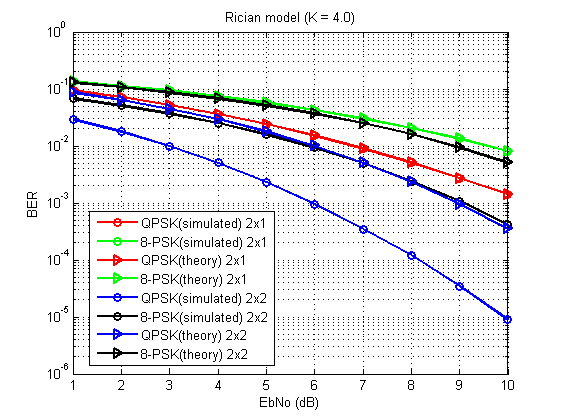\n",
157 | ">*Fig. 2. Bit-error ratio performance for simulated partly time invariant MISO and MIMO channels (light shadowing)*\n",
158 | "\n",
159 | "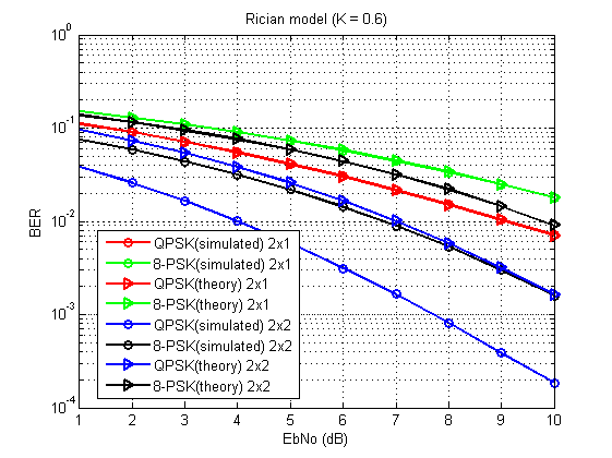\n",
160 | ">*Fig. 3. Bit-error ratio performance for simulated partly time invariant MISO and MIMO channels (strong shadowing)*\n",
161 | "\n",
162 | "Note that the case of Alamouti 2x1 completely matched with the theoretical 2nd order **diversity**, however Alamouti 2x2 has the better BER performance due to additional **array gain**."
163 | ]
164 | },
165 | {
166 | "cell_type": "markdown",
167 | "metadata": {},
168 | "source": [
169 | "# Tarokh codes\n",
170 | "\n",
171 | "As you may mention, Alamouti is the case when we have only two transmitt antennas ($M_T=2$). However other configurations are also available. For example, according to \\[2\\]:\n",
172 | "\n",
173 | "
\n",
96 | "\n",
97 | "where $c_i$ is the input symbols ($i=1,2$), $t_i$ is the certain timeslot ($i=1,2$) and $\\mathbf{S}$ is the transmission matrix. "
98 | ]
99 | },
100 | {
101 | "cell_type": "markdown",
102 | "metadata": {},
103 | "source": [
104 | "Alamouti scheme is **ortogonal** [1, p.93-95, 97-98] and does not require the channel state information.\n",
105 | "\n",
106 | "> **Task for the self-education**:\n",
107 | ">\n",
108 | "> Learn more about other transmission cases: \n",
109 | "> * receiver side diversity - Rx-MRC (Maximum Ratio Combining);\n",
110 | "> * transmitter side diversity (channel is known for the transmitter) - Tx-MRC;\n",
111 | "> * MIMO case (channel is known for the transmitter) - DET (Dominant Eigenmode Transmission)\n",
112 | "\n",
113 | "\n",
114 | ""
115 | ]
116 | },
117 | {
118 | "cell_type": "markdown",
119 | "metadata": {},
120 | "source": [
121 | "# MATLAB Simulation"
122 | ]
123 | },
124 | {
125 | "cell_type": "markdown",
126 | "metadata": {},
127 | "source": [
128 | "The following blocks (objects) can be used to simulate Alamouti transmission:\n",
129 | "\n",
130 | "* [comm.OSTBCEncoder](https://www.mathworks.com/help/comm/ref/comm.ostbcencoder-system-object.html?s_tid=doc_ta) - Ortogonal Space-Time Block Codes Encoder (Communications ToolBox);\n",
131 | "\n",
132 | "* [comm.OSTBCCombiner](https://www.mathworks.com/help/comm/ref/comm.ostbccombiner-system-object.html) - Ortogonal Space-Time Block Codes Combiner (Communications ToolBox);\n",
133 | "\n",
134 | "> **NOTE THAT**:\n",
135 | ">\n",
136 | "> According to [1, p.113] $r = \\frac{N}{T}$ (the spatial code rate defined as the average number of independent symbols (constructed from the N input symbols) transmitted from the $M_T$ antennas over $T$ symbol periods). E.g, for Alamouti scheme $r$ = 1.\n",
137 | ">\n",
138 | "> However, MathWorks use [another formula](https://www.mathworks.com/help/comm/ref/ostbcencoder.html) for similar variable.\n",
139 | "\n",
140 | "The channel was simulated according to the following tutorial: [Introduction to MIMO Systems](https://www.mathworks.com/help/comm/examples/introduction-to-mimo-systems.html), i.e. the channel is the invariant during the couple of snapshots (in other words, during the one Alamouti symbol transmission)."
141 | ]
142 | },
143 | {
144 | "cell_type": "markdown",
145 | "metadata": {},
146 | "source": [
147 | "**Simulation script**:\n",
148 | "\n",
149 | "> Vladimir Fadeev (2019). Alamouti over Rician flat fading channel (https://www.mathworks.com/matlabcentral/fileexchange/70557-alamouti-over-rician-flat-fading-channel), MATLAB Central File Exchange. Retrieved October 7, 2019."
150 | ]
151 | },
152 | {
153 | "cell_type": "markdown",
154 | "metadata": {},
155 | "source": [
156 | "\n",
157 | ">*Fig. 2. Bit-error ratio performance for simulated partly time invariant MISO and MIMO channels (light shadowing)*\n",
158 | "\n",
159 | "\n",
160 | ">*Fig. 3. Bit-error ratio performance for simulated partly time invariant MISO and MIMO channels (strong shadowing)*\n",
161 | "\n",
162 | "Note that the case of Alamouti 2x1 completely matched with the theoretical 2nd order **diversity**, however Alamouti 2x2 has the better BER performance due to additional **array gain**."
163 | ]
164 | },
165 | {
166 | "cell_type": "markdown",
167 | "metadata": {},
168 | "source": [
169 | "# Tarokh codes\n",
170 | "\n",
171 | "As you may mention, Alamouti is the case when we have only two transmitt antennas ($M_T=2$). However other configurations are also available. For example, according to \\[2\\]:\n",
172 | "\n",
173 | " \n",
174 | "\n",
175 | "> *Fig. 4. Transmission schemes of the $M_T=3$ and $M_T=4$ cases \\[2\\].*\n",
176 | "\n",
177 | "Actually, these codes require the same routines for the encoding and decoding as the Alamouti code and therefore they are collected into the **Ortogonal Space-Time Codes** term. \n"
178 | ]
179 | },
180 | {
181 | "cell_type": "markdown",
182 | "metadata": {},
183 | "source": [
184 | "# References\n",
185 | "\n",
186 | "1. Paulraj, Arogyaswami, Rohit Nabar, and Dhananjay Gore. Introduction to space-time wireless communications. Cambridge university press, 2003.\n",
187 | "\n",
188 | "2. Tarokh, V., Jafarkhani, H., & Calderbank, A. R. (1999). Space-time block codes from orthogonal designs. IEEE Transactions on Information theory, 45(5), 1456-1467.\n",
189 | "\n",
190 | "# Suggested literature\n",
191 | "\n",
192 | "1. Tiwari, K., & Saini, D. S. (2014, December). BER performance comparison of MIMO system with STBC and MRC over different fading channels. In High Performance Computing and Applications (ICHPCA), 2014 International Conference on (pp. 1-6). IEEE.\n",
193 | "\n"
194 | ]
195 | }
196 | ],
197 | "metadata": {
198 | "kernelspec": {
199 | "display_name": "Python 3",
200 | "language": "python",
201 | "name": "python3"
202 | },
203 | "language_info": {
204 | "codemirror_mode": {
205 | "name": "ipython",
206 | "version": 3
207 | },
208 | "file_extension": ".py",
209 | "mimetype": "text/x-python",
210 | "name": "python",
211 | "nbconvert_exporter": "python",
212 | "pygments_lexer": "ipython3",
213 | "version": "3.7.4"
214 | }
215 | },
216 | "nbformat": 4,
217 | "nbformat_minor": 2
218 | }
219 |
--------------------------------------------------------------------------------
/MIMO/RicianFlatFadingMATLAB.ipynb:
--------------------------------------------------------------------------------
1 | {
2 | "cells": [
3 | {
4 | "cell_type": "markdown",
5 | "metadata": {},
6 | "source": [
7 | "# Rician flat fading channel modeling\n",
8 | "## (MATLAB tutorial)\n",
9 | "### M.Sc. Vladimir Fadeev\n",
10 | "#### Kazan, 30.11.2018"
11 | ]
12 | },
13 | {
14 | "cell_type": "markdown",
15 | "metadata": {},
16 | "source": [
17 | "## Preface\n",
18 | "\n",
19 | "Multiple Input Multiple Output (MIMO) system with linear arrays will be considered during this research. \n",
20 | "\n",
21 | "Why MIMO?\n",
22 | "\n",
23 | "Firstly, MIMO thechnology is the part of [LTE and LTE-A standards](https://gsmcommunications.blogspot.ru/2011/04/lte-long-term-evolution-phy-overview.html) that motivates us to learn little bit more about this.\n",
24 | "\n",
25 | "Moreover, we are considering MIMO system as the example of generalized communication system which can be easily simplified to more specific cases: MISO (Multiple Input Single Output), SIMO (Single Input Multiple Output) and SISO (Single Input Single Output).\n",
26 | "\n",
27 | "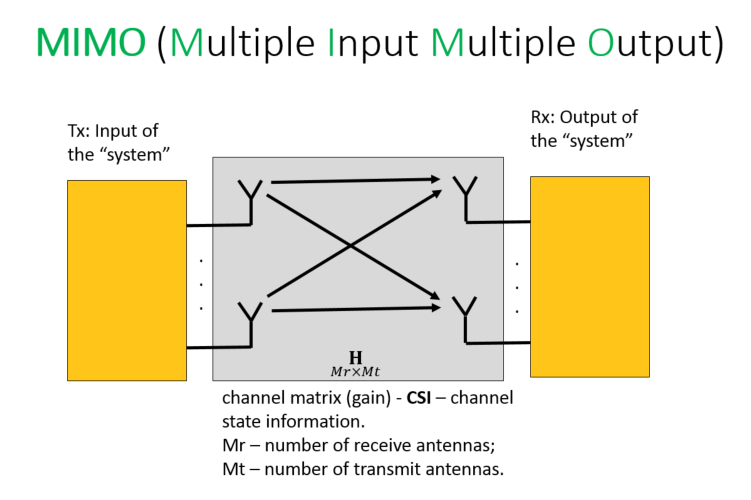\n",
28 | "\n",
29 | "More coplicated models should be researched for Massive MIMO technology (5G) and reqtangular antenna arrays cases."
30 | ]
31 | },
32 | {
33 | "cell_type": "markdown",
34 | "metadata": {},
35 | "source": [
36 | "## Introduction"
37 | ]
38 | },
39 | {
40 | "cell_type": "markdown",
41 | "metadata": {},
42 | "source": [
43 | "Let us start from the small theory explanation \\[1, p. 11-12\\]:\n",
44 | "\n",
45 | "> A signal propagating through the wireless channel arrives at the destination along a number of different paths, collectively referred to as multipath. These paths arise from scattering, reflection and diffraction of the radiated energy by objects in the environment or refraction in the medium. The different propagation mechanisms influence path loss and fading models differently. However, for convenience we refer to all these distorting mechanisms as “scattering”. Further, throughout the book, we assume a complex baseband representation for the signal and channel unless otherwise specified.\n",
46 | ">\n",
47 | "> The signal power drops off due to three effects: mean propagation (path) loss, macroscopic fading and microscopic fading. The mean propagation loss in macrocellular environments comes from inverse square law power loss, absorption by water and foliage and the effect of ground reflection. Mean propagation loss is range dependent.\n",
48 | ">\n",
49 | "> Macroscopic fading results from a blocking effect by buildings and natural features and is also known as long term fading or shadowing. Microscopic fading results from the constructive and destructive combination of multipaths and is also known as short term fading or fast fading. Multipath propagation results in the spreading of the signal in different dimensions. These are delay spread, Doppler (or frequency) spread (this needs a time-varying multipath channel) and angle spread. These spreads have significant effects on the signal. Mean path loss, macroscopic fading, microscopic fading, delay spread, Doppler spread and angle spread are the main channel effects and are described below.\n",
50 | "\n",
51 | "
\n",
174 | "\n",
175 | "> *Fig. 4. Transmission schemes of the $M_T=3$ and $M_T=4$ cases \\[2\\].*\n",
176 | "\n",
177 | "Actually, these codes require the same routines for the encoding and decoding as the Alamouti code and therefore they are collected into the **Ortogonal Space-Time Codes** term. \n"
178 | ]
179 | },
180 | {
181 | "cell_type": "markdown",
182 | "metadata": {},
183 | "source": [
184 | "# References\n",
185 | "\n",
186 | "1. Paulraj, Arogyaswami, Rohit Nabar, and Dhananjay Gore. Introduction to space-time wireless communications. Cambridge university press, 2003.\n",
187 | "\n",
188 | "2. Tarokh, V., Jafarkhani, H., & Calderbank, A. R. (1999). Space-time block codes from orthogonal designs. IEEE Transactions on Information theory, 45(5), 1456-1467.\n",
189 | "\n",
190 | "# Suggested literature\n",
191 | "\n",
192 | "1. Tiwari, K., & Saini, D. S. (2014, December). BER performance comparison of MIMO system with STBC and MRC over different fading channels. In High Performance Computing and Applications (ICHPCA), 2014 International Conference on (pp. 1-6). IEEE.\n",
193 | "\n"
194 | ]
195 | }
196 | ],
197 | "metadata": {
198 | "kernelspec": {
199 | "display_name": "Python 3",
200 | "language": "python",
201 | "name": "python3"
202 | },
203 | "language_info": {
204 | "codemirror_mode": {
205 | "name": "ipython",
206 | "version": 3
207 | },
208 | "file_extension": ".py",
209 | "mimetype": "text/x-python",
210 | "name": "python",
211 | "nbconvert_exporter": "python",
212 | "pygments_lexer": "ipython3",
213 | "version": "3.7.4"
214 | }
215 | },
216 | "nbformat": 4,
217 | "nbformat_minor": 2
218 | }
219 |
--------------------------------------------------------------------------------
/MIMO/RicianFlatFadingMATLAB.ipynb:
--------------------------------------------------------------------------------
1 | {
2 | "cells": [
3 | {
4 | "cell_type": "markdown",
5 | "metadata": {},
6 | "source": [
7 | "# Rician flat fading channel modeling\n",
8 | "## (MATLAB tutorial)\n",
9 | "### M.Sc. Vladimir Fadeev\n",
10 | "#### Kazan, 30.11.2018"
11 | ]
12 | },
13 | {
14 | "cell_type": "markdown",
15 | "metadata": {},
16 | "source": [
17 | "## Preface\n",
18 | "\n",
19 | "Multiple Input Multiple Output (MIMO) system with linear arrays will be considered during this research. \n",
20 | "\n",
21 | "Why MIMO?\n",
22 | "\n",
23 | "Firstly, MIMO thechnology is the part of [LTE and LTE-A standards](https://gsmcommunications.blogspot.ru/2011/04/lte-long-term-evolution-phy-overview.html) that motivates us to learn little bit more about this.\n",
24 | "\n",
25 | "Moreover, we are considering MIMO system as the example of generalized communication system which can be easily simplified to more specific cases: MISO (Multiple Input Single Output), SIMO (Single Input Multiple Output) and SISO (Single Input Single Output).\n",
26 | "\n",
27 | "\n",
28 | "\n",
29 | "More coplicated models should be researched for Massive MIMO technology (5G) and reqtangular antenna arrays cases."
30 | ]
31 | },
32 | {
33 | "cell_type": "markdown",
34 | "metadata": {},
35 | "source": [
36 | "## Introduction"
37 | ]
38 | },
39 | {
40 | "cell_type": "markdown",
41 | "metadata": {},
42 | "source": [
43 | "Let us start from the small theory explanation \\[1, p. 11-12\\]:\n",
44 | "\n",
45 | "> A signal propagating through the wireless channel arrives at the destination along a number of different paths, collectively referred to as multipath. These paths arise from scattering, reflection and diffraction of the radiated energy by objects in the environment or refraction in the medium. The different propagation mechanisms influence path loss and fading models differently. However, for convenience we refer to all these distorting mechanisms as “scattering”. Further, throughout the book, we assume a complex baseband representation for the signal and channel unless otherwise specified.\n",
46 | ">\n",
47 | "> The signal power drops off due to three effects: mean propagation (path) loss, macroscopic fading and microscopic fading. The mean propagation loss in macrocellular environments comes from inverse square law power loss, absorption by water and foliage and the effect of ground reflection. Mean propagation loss is range dependent.\n",
48 | ">\n",
49 | "> Macroscopic fading results from a blocking effect by buildings and natural features and is also known as long term fading or shadowing. Microscopic fading results from the constructive and destructive combination of multipaths and is also known as short term fading or fast fading. Multipath propagation results in the spreading of the signal in different dimensions. These are delay spread, Doppler (or frequency) spread (this needs a time-varying multipath channel) and angle spread. These spreads have significant effects on the signal. Mean path loss, macroscopic fading, microscopic fading, delay spread, Doppler spread and angle spread are the main channel effects and are described below.\n",
50 | "\n",
51 | " \n",
52 | "\n",
53 | "> *Fig.1. Signal power fluctuation vs range in wireless channels. Mean propagation loss increases\n",
54 | "monotonically with range. Local deviations may occur due to macroscopic and microscopic fading \\[1, p.14\\].*\n",
55 | "\n",
56 | "So, firstly, the fading process can be classified based on appearence reasons:\n",
57 | "\n",
58 | "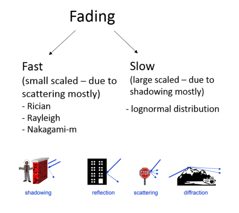\n",
59 | "\n",
60 | "\n",
61 | "However, fading can also be classified in dependence on channel characteristics: [coherence time](https://en.wikipedia.org/wiki/Coherence_time_(communications_systems)) of the channel $T_c$ and [coherence bandwidth](https://en.wikipedia.org/wiki/Coherence_bandwidth) $B_c$:\n",
62 | "\n",
63 | "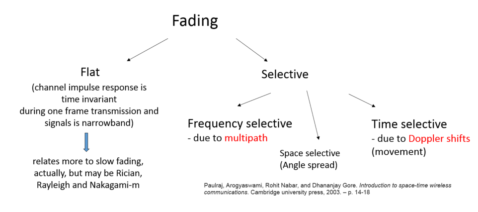\n",
64 | "\n",
65 | "Only flat fading is considered during this research."
66 | ]
67 | },
68 | {
69 | "cell_type": "markdown",
70 | "metadata": {},
71 | "source": [
72 | "### What is the requirement to be frequency-flat?\n",
73 | "\n",
74 | "To obtain frequency-flat transmission the signal ***bit rate*** ($W = \\Delta f$) should not exceed [coherence bandwidth](https://en.wikipedia.org/wiki/Coherence_bandwidth).\n",
75 | "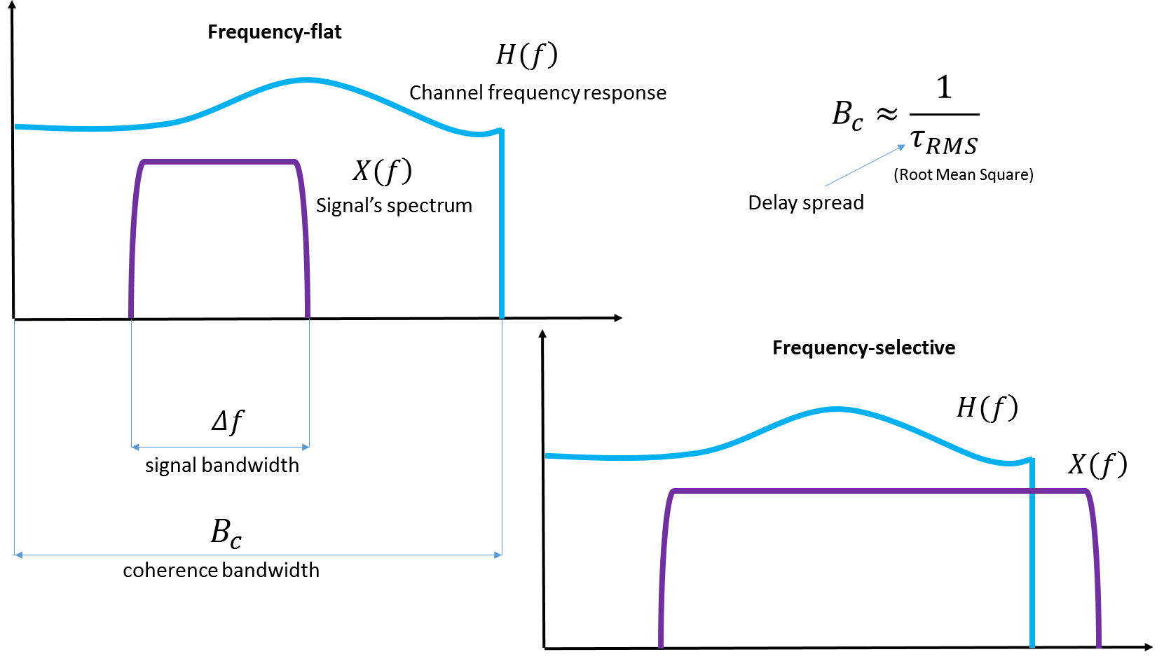\n"
76 | ]
77 | },
78 | {
79 | "cell_type": "markdown",
80 | "metadata": {},
81 | "source": [
82 | "### What is the requirement to be time invarinat?\n",
83 | "\n",
84 | "To obtain frequency-flat transmission the signal ***duration*** ($T = \\frac{1}{W}$) should not exceed [coherence time](https://en.wikipedia.org/wiki/https://en.wikipedia.org/wiki/Coherence_time).\n",
85 | "
\n",
52 | "\n",
53 | "> *Fig.1. Signal power fluctuation vs range in wireless channels. Mean propagation loss increases\n",
54 | "monotonically with range. Local deviations may occur due to macroscopic and microscopic fading \\[1, p.14\\].*\n",
55 | "\n",
56 | "So, firstly, the fading process can be classified based on appearence reasons:\n",
57 | "\n",
58 | "\n",
59 | "\n",
60 | "\n",
61 | "However, fading can also be classified in dependence on channel characteristics: [coherence time](https://en.wikipedia.org/wiki/Coherence_time_(communications_systems)) of the channel $T_c$ and [coherence bandwidth](https://en.wikipedia.org/wiki/Coherence_bandwidth) $B_c$:\n",
62 | "\n",
63 | "\n",
64 | "\n",
65 | "Only flat fading is considered during this research."
66 | ]
67 | },
68 | {
69 | "cell_type": "markdown",
70 | "metadata": {},
71 | "source": [
72 | "### What is the requirement to be frequency-flat?\n",
73 | "\n",
74 | "To obtain frequency-flat transmission the signal ***bit rate*** ($W = \\Delta f$) should not exceed [coherence bandwidth](https://en.wikipedia.org/wiki/Coherence_bandwidth).\n",
75 | "\n"
76 | ]
77 | },
78 | {
79 | "cell_type": "markdown",
80 | "metadata": {},
81 | "source": [
82 | "### What is the requirement to be time invarinat?\n",
83 | "\n",
84 | "To obtain frequency-flat transmission the signal ***duration*** ($T = \\frac{1}{W}$) should not exceed [coherence time](https://en.wikipedia.org/wiki/https://en.wikipedia.org/wiki/Coherence_time).\n",
85 | " \n"
86 | ]
87 | },
88 | {
89 | "cell_type": "markdown",
90 | "metadata": {},
91 | "source": [
92 | "### Sugested literature \n",
93 | "* Goldsmith A. Wireless communications. – Cambridge university press, 2005. – p. 88-92\n",
94 | "\n",
95 | "* Kanatas A. G., Panagopoulos A. D. (ed.). Radio Wave Propagation and Channel Modeling for Earth–Space Systems. – CRC Press, 2016. - p. 107"
96 | ]
97 | },
98 | {
99 | "cell_type": "markdown",
100 | "metadata": {},
101 | "source": [
102 | "## Generalized Channel model"
103 | ]
104 | },
105 | {
106 | "cell_type": "markdown",
107 | "metadata": {},
108 | "source": [
109 | "Rician flat uncorrelated fading channel can be estimated based on described in [\\[2\\]](https://pdfs.semanticscholar.org/0fdd/65ed5a4e90f2ee44a1a0a8caa3f7021ce9f9.pdf) math model (MIMO system with linear arrays):\n",
110 | "\n",
111 | "$$\n",
112 | "\\mathbf{H} = \\sqrt{\\frac{K}{K+1}}\\mathbf{H_{LoS}} + \\sqrt{\\frac{1} {K+1}}\\mathbf{H_{NLoS}} \\qquad (1)\n",
113 | "$$\n",
114 | "\n",
115 | "where $\\mathbf{H}$ is the channel matrix, $K$ is the Rician factor, $\\mathbf{H_{LoS}}$ is the Line-of-Sight component and $\\mathbf{H_{NLoS}}$ is the Non-Line-of-Sight component.\n",
116 | "\n"
117 | ]
118 | },
119 | {
120 | "cell_type": "markdown",
121 | "metadata": {},
122 | "source": [
123 | "## Line-of-Sight component"
124 | ]
125 | },
126 | {
127 | "cell_type": "markdown",
128 | "metadata": {},
129 | "source": [
130 | "The term $\\sqrt{\\frac{K}{K+1}}\\mathbf{H}_{LoS} = E\\{H\\}$ represents the mean component of the channel matrix and can be modeled according to geometrical approach:\n",
131 | "\n",
132 | "$$\\mathbf{H}_{LoS} = \\mathbf{a}_R(\\theta_R)\\mathbf{a}_T(\\theta_T)^H \\qquad (2)$$ \n",
133 | "\n",
134 | "where $\\mathbf{a}_R(\\theta_R)$ and $\\mathbf{a}_T(\\theta_T)$ are the receive array and transmitt array responses, and $\\theta_R$ and $\\theta_T$ are the angls of arrival and departure."
135 | ]
136 | },
137 | {
138 | "cell_type": "markdown",
139 | "metadata": {},
140 | "source": [
141 | "Array response can be expressed as: \n",
142 | "$$ \\mathbf{a} = \\left[1, e^{j2\\pi d cos(\\theta)},..., e^{j2\\pi d(N-1) cos(\\theta)} \\right] \\qquad (3)$$\n",
143 | "\n",
144 | "where $d$ is the antenna spacing in wavelenghts, $N$ is the number of the array elements. "
145 | ]
146 | },
147 | {
148 | "cell_type": "markdown",
149 | "metadata": {},
150 | "source": [
151 | "
\n"
86 | ]
87 | },
88 | {
89 | "cell_type": "markdown",
90 | "metadata": {},
91 | "source": [
92 | "### Sugested literature \n",
93 | "* Goldsmith A. Wireless communications. – Cambridge university press, 2005. – p. 88-92\n",
94 | "\n",
95 | "* Kanatas A. G., Panagopoulos A. D. (ed.). Radio Wave Propagation and Channel Modeling for Earth–Space Systems. – CRC Press, 2016. - p. 107"
96 | ]
97 | },
98 | {
99 | "cell_type": "markdown",
100 | "metadata": {},
101 | "source": [
102 | "## Generalized Channel model"
103 | ]
104 | },
105 | {
106 | "cell_type": "markdown",
107 | "metadata": {},
108 | "source": [
109 | "Rician flat uncorrelated fading channel can be estimated based on described in [\\[2\\]](https://pdfs.semanticscholar.org/0fdd/65ed5a4e90f2ee44a1a0a8caa3f7021ce9f9.pdf) math model (MIMO system with linear arrays):\n",
110 | "\n",
111 | "$$\n",
112 | "\\mathbf{H} = \\sqrt{\\frac{K}{K+1}}\\mathbf{H_{LoS}} + \\sqrt{\\frac{1} {K+1}}\\mathbf{H_{NLoS}} \\qquad (1)\n",
113 | "$$\n",
114 | "\n",
115 | "where $\\mathbf{H}$ is the channel matrix, $K$ is the Rician factor, $\\mathbf{H_{LoS}}$ is the Line-of-Sight component and $\\mathbf{H_{NLoS}}$ is the Non-Line-of-Sight component.\n",
116 | "\n"
117 | ]
118 | },
119 | {
120 | "cell_type": "markdown",
121 | "metadata": {},
122 | "source": [
123 | "## Line-of-Sight component"
124 | ]
125 | },
126 | {
127 | "cell_type": "markdown",
128 | "metadata": {},
129 | "source": [
130 | "The term $\\sqrt{\\frac{K}{K+1}}\\mathbf{H}_{LoS} = E\\{H\\}$ represents the mean component of the channel matrix and can be modeled according to geometrical approach:\n",
131 | "\n",
132 | "$$\\mathbf{H}_{LoS} = \\mathbf{a}_R(\\theta_R)\\mathbf{a}_T(\\theta_T)^H \\qquad (2)$$ \n",
133 | "\n",
134 | "where $\\mathbf{a}_R(\\theta_R)$ and $\\mathbf{a}_T(\\theta_T)$ are the receive array and transmitt array responses, and $\\theta_R$ and $\\theta_T$ are the angls of arrival and departure."
135 | ]
136 | },
137 | {
138 | "cell_type": "markdown",
139 | "metadata": {},
140 | "source": [
141 | "Array response can be expressed as: \n",
142 | "$$ \\mathbf{a} = \\left[1, e^{j2\\pi d cos(\\theta)},..., e^{j2\\pi d(N-1) cos(\\theta)} \\right] \\qquad (3)$$\n",
143 | "\n",
144 | "where $d$ is the antenna spacing in wavelenghts, $N$ is the number of the array elements. "
145 | ]
146 | },
147 | {
148 | "cell_type": "markdown",
149 | "metadata": {},
150 | "source": [
151 | " \n",
152 | "\n",
153 | "> *Fig. 2. [Linear array geometry](http://www.waves.toronto.edu/prof/svhum/ece422/notes/15-arrays2.pdf).* \n",
154 | "\n",
155 | "\n",
156 | "### Task: \n",
157 | "What is the squared Frobenius norm of the LoS component?\n"
158 | ]
159 | },
160 | {
161 | "cell_type": "markdown",
162 | "metadata": {},
163 | "source": [
164 | "## Non-LoS componenet"
165 | ]
166 | },
167 | {
168 | "cell_type": "markdown",
169 | "metadata": {},
170 | "source": [
171 | "NLoS component can be classicaly modeled as the matrix of **IID** (independent identicaly distributed) **ZMCSCG** (zero mean\n",
172 | "circularly symmetric complex Gaussian) random values (amplitudes) [1, p. 39]:\n",
173 | "\n",
174 | "$$ Z = X + jY \\qquad (4)$$\n",
175 | "\n",
176 | "where $X \\sim \\mathcal{N}(0,\\,\\sigma^2)$ and $Y \\sim \\mathcal{N}(0,\\,\\sigma^2)$. Frequently, the model with normalized average power is used, such that:\n",
177 | "\n",
178 | "$$ var\\{Z\\} = E\\{\\left|Z\\right|^2\\} = 1 \\qquad (5)$$\n",
179 | "\n",
180 | "Hence, $Z \\sim \\mathcal{N}(0,\\,1)$. Moreover, for independent distortions of both in-phase and quadrature signal components envolope can be described as the Rayleigh process \\[3, p.78\\]: \n",
181 | "\n",
182 | "$$ Z = \\sqrt{\\hat{X}^2 + \\hat{Y}^2} \\qquad (6)$$\n",
183 | "\n",
184 | "where $\\hat{X} \\sim \\mathcal{N}(0,\\,\\sigma^2)$ and $\\hat{Y} \\sim \\mathcal{N}(0,\\,\\sigma^2)$.\n",
185 | "\n",
186 | "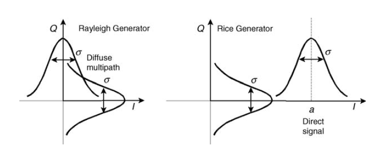\n",
187 | "> *Fig. 3. Gaussian generators in quadrature for simulating Rayleigh and Rice fades [\\[4, p.125\\]](https://s3.amazonaws.com/academia.edu.documents/45934974/Modelling.the.Wireless.Propagation.Channel.A.simulation.approach.with.Matlab.pdf?AWSAccessKeyId=AKIAIWOWYYGZ2Y53UL3A&Expires=1542970346&Signature=IkBGDMI6ref5QrEwFz2RG6Ns7vI%3D&response-content-disposition=inline%3B%20filename%3DModelling.the.Wireless.Propagation.Chann.pdf)*\n",
188 | "\n",
189 | "Actually, these phenomena mean Rayleigh fading (spatialy white) channel with scale factor $ \\sigma = \\frac{1}{\\sqrt{2}} $ which can be modeled as [\\[4, p.125\\]](https://s3.amazonaws.com/academia.edu.documents/45934974/Modelling.the.Wireless.Propagation.Channel.A.simulation.approach.with.Matlab.pdf?AWSAccessKeyId=AKIAIWOWYYGZ2Y53UL3A&Expires=1542970346&Signature=IkBGDMI6ref5QrEwFz2RG6Ns7vI%3D&response-content-disposition=inline%3B%20filename%3DModelling.the.Wireless.Propagation.Chann.pdf):\n",
190 | "\n",
191 | "$$ \\mathbf{H}_{NLoS} = \\sqrt{\\frac{1}{2}}\\left(G_1+jG_2\\right) \\qquad (7)$$\n",
192 | "\n",
193 | "where $\\mathbf{G}_1 \\sim \\mathcal{N}(0,\\,1)$ and $\\mathbf{G}_2 \\sim \\mathcal{N}(0,\\,1)$ are consisting of the normaly distributed values matrices."
194 | ]
195 | },
196 | {
197 | "cell_type": "markdown",
198 | "metadata": {},
199 | "source": [
200 | "## Single antenna simplification"
201 | ]
202 | },
203 | {
204 | "cell_type": "markdown",
205 | "metadata": {},
206 | "source": [
207 | "Channel model with simplification to **SISO** case will have the following form:\n",
208 | "\n",
209 | "$$\n",
210 | "h = \\sqrt{\\frac{K}{K+1}} + \\sqrt{\\frac{1}{2(K+1)}}\\left(G_1+jG_2\\right) \\qquad (8)\n",
211 | "$$\n",
212 | "\n",
213 | "And can be described via the following figure:\n",
214 | "\n",
215 | "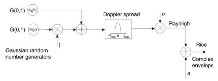\n",
216 | "> *Fig.4. Schematic diagram of the Rayleigh/Rice simulator (narrowband channel) [\\[4, p.127\\]](https://s3.amazonaws.com/academia.edu.documents/45934974/Modelling.the.Wireless.Propagation.Channel.A.simulation.approach.with.Matlab.pdf?AWSAccessKeyId=AKIAIWOWYYGZ2Y53UL3A&Expires=1542970346&Signature=IkBGDMI6ref5QrEwFz2RG6Ns7vI%3D&response-content-disposition=inline%3B%20filename%3DModelling.the.Wireless.Propagation.Chann.pdf)*.\n",
217 | "\n",
218 | "where $\\sigma = \\sqrt{\\frac{1}{2(K+1)}}$ is Rician scale parameter and $a = \\sqrt{\\frac{K}{K+1}} $ is the Rician noncentrality parameter. \n",
219 | "\n",
220 | "> **NOTE THAT**: \n",
221 | ">\n",
222 | ">We are considering the flat fading channel and therefore assume Doppler spreadimpact as neglectable."
223 | ]
224 | },
225 | {
226 | "cell_type": "markdown",
227 | "metadata": {},
228 | "source": [
229 | "> **NOTE THAT**:\n",
230 | ">\n",
231 | "> Classical Additive White Gaussian Noise \\(AWGN\\) model was selected (complex signal case) for the modeling of an additive noise. Nice explanation can be found via the [following link](https://www.gaussianwaves.com/2015/06/how-to-generate-awgn-noise-in-matlaboctave-without-using-in-built-awgn-function/).\n"
232 | ]
233 | },
234 | {
235 | "cell_type": "markdown",
236 | "metadata": {},
237 | "source": [
238 | "> **NOTE THAT**:\n",
239 | ">\n",
240 | ">The method how to estimate ergodic capacity usung the channel model can be obtained via the [following link](https://www.gaussianwaves.com/2014/09/ergodic-capacity-of-a-siso-system-over-a-rayleigh-fading-channel-simulation-in-matlab/)."
241 | ]
242 | },
243 | {
244 | "cell_type": "markdown",
245 | "metadata": {},
246 | "source": [
247 | "## Model verification\n",
248 | "\n",
249 | "For verification of the proposal model we model random binary message \\(length of the message equals to 100000 bits\\), modulate it by M-PSK / M-QAM (Gray mapping rule), multiply elementwise with fading process, add white gaussian noise, equalize by Zero-Forcing method, demodulate and calculate BER. The number of trials is equal to 100.\n",
250 | "\n",
251 | "
\n",
152 | "\n",
153 | "> *Fig. 2. [Linear array geometry](http://www.waves.toronto.edu/prof/svhum/ece422/notes/15-arrays2.pdf).* \n",
154 | "\n",
155 | "\n",
156 | "### Task: \n",
157 | "What is the squared Frobenius norm of the LoS component?\n"
158 | ]
159 | },
160 | {
161 | "cell_type": "markdown",
162 | "metadata": {},
163 | "source": [
164 | "## Non-LoS componenet"
165 | ]
166 | },
167 | {
168 | "cell_type": "markdown",
169 | "metadata": {},
170 | "source": [
171 | "NLoS component can be classicaly modeled as the matrix of **IID** (independent identicaly distributed) **ZMCSCG** (zero mean\n",
172 | "circularly symmetric complex Gaussian) random values (amplitudes) [1, p. 39]:\n",
173 | "\n",
174 | "$$ Z = X + jY \\qquad (4)$$\n",
175 | "\n",
176 | "where $X \\sim \\mathcal{N}(0,\\,\\sigma^2)$ and $Y \\sim \\mathcal{N}(0,\\,\\sigma^2)$. Frequently, the model with normalized average power is used, such that:\n",
177 | "\n",
178 | "$$ var\\{Z\\} = E\\{\\left|Z\\right|^2\\} = 1 \\qquad (5)$$\n",
179 | "\n",
180 | "Hence, $Z \\sim \\mathcal{N}(0,\\,1)$. Moreover, for independent distortions of both in-phase and quadrature signal components envolope can be described as the Rayleigh process \\[3, p.78\\]: \n",
181 | "\n",
182 | "$$ Z = \\sqrt{\\hat{X}^2 + \\hat{Y}^2} \\qquad (6)$$\n",
183 | "\n",
184 | "where $\\hat{X} \\sim \\mathcal{N}(0,\\,\\sigma^2)$ and $\\hat{Y} \\sim \\mathcal{N}(0,\\,\\sigma^2)$.\n",
185 | "\n",
186 | "\n",
187 | "> *Fig. 3. Gaussian generators in quadrature for simulating Rayleigh and Rice fades [\\[4, p.125\\]](https://s3.amazonaws.com/academia.edu.documents/45934974/Modelling.the.Wireless.Propagation.Channel.A.simulation.approach.with.Matlab.pdf?AWSAccessKeyId=AKIAIWOWYYGZ2Y53UL3A&Expires=1542970346&Signature=IkBGDMI6ref5QrEwFz2RG6Ns7vI%3D&response-content-disposition=inline%3B%20filename%3DModelling.the.Wireless.Propagation.Chann.pdf)*\n",
188 | "\n",
189 | "Actually, these phenomena mean Rayleigh fading (spatialy white) channel with scale factor $ \\sigma = \\frac{1}{\\sqrt{2}} $ which can be modeled as [\\[4, p.125\\]](https://s3.amazonaws.com/academia.edu.documents/45934974/Modelling.the.Wireless.Propagation.Channel.A.simulation.approach.with.Matlab.pdf?AWSAccessKeyId=AKIAIWOWYYGZ2Y53UL3A&Expires=1542970346&Signature=IkBGDMI6ref5QrEwFz2RG6Ns7vI%3D&response-content-disposition=inline%3B%20filename%3DModelling.the.Wireless.Propagation.Chann.pdf):\n",
190 | "\n",
191 | "$$ \\mathbf{H}_{NLoS} = \\sqrt{\\frac{1}{2}}\\left(G_1+jG_2\\right) \\qquad (7)$$\n",
192 | "\n",
193 | "where $\\mathbf{G}_1 \\sim \\mathcal{N}(0,\\,1)$ and $\\mathbf{G}_2 \\sim \\mathcal{N}(0,\\,1)$ are consisting of the normaly distributed values matrices."
194 | ]
195 | },
196 | {
197 | "cell_type": "markdown",
198 | "metadata": {},
199 | "source": [
200 | "## Single antenna simplification"
201 | ]
202 | },
203 | {
204 | "cell_type": "markdown",
205 | "metadata": {},
206 | "source": [
207 | "Channel model with simplification to **SISO** case will have the following form:\n",
208 | "\n",
209 | "$$\n",
210 | "h = \\sqrt{\\frac{K}{K+1}} + \\sqrt{\\frac{1}{2(K+1)}}\\left(G_1+jG_2\\right) \\qquad (8)\n",
211 | "$$\n",
212 | "\n",
213 | "And can be described via the following figure:\n",
214 | "\n",
215 | "\n",
216 | "> *Fig.4. Schematic diagram of the Rayleigh/Rice simulator (narrowband channel) [\\[4, p.127\\]](https://s3.amazonaws.com/academia.edu.documents/45934974/Modelling.the.Wireless.Propagation.Channel.A.simulation.approach.with.Matlab.pdf?AWSAccessKeyId=AKIAIWOWYYGZ2Y53UL3A&Expires=1542970346&Signature=IkBGDMI6ref5QrEwFz2RG6Ns7vI%3D&response-content-disposition=inline%3B%20filename%3DModelling.the.Wireless.Propagation.Chann.pdf)*.\n",
217 | "\n",
218 | "where $\\sigma = \\sqrt{\\frac{1}{2(K+1)}}$ is Rician scale parameter and $a = \\sqrt{\\frac{K}{K+1}} $ is the Rician noncentrality parameter. \n",
219 | "\n",
220 | "> **NOTE THAT**: \n",
221 | ">\n",
222 | ">We are considering the flat fading channel and therefore assume Doppler spreadimpact as neglectable."
223 | ]
224 | },
225 | {
226 | "cell_type": "markdown",
227 | "metadata": {},
228 | "source": [
229 | "> **NOTE THAT**:\n",
230 | ">\n",
231 | "> Classical Additive White Gaussian Noise \\(AWGN\\) model was selected (complex signal case) for the modeling of an additive noise. Nice explanation can be found via the [following link](https://www.gaussianwaves.com/2015/06/how-to-generate-awgn-noise-in-matlaboctave-without-using-in-built-awgn-function/).\n"
232 | ]
233 | },
234 | {
235 | "cell_type": "markdown",
236 | "metadata": {},
237 | "source": [
238 | "> **NOTE THAT**:\n",
239 | ">\n",
240 | ">The method how to estimate ergodic capacity usung the channel model can be obtained via the [following link](https://www.gaussianwaves.com/2014/09/ergodic-capacity-of-a-siso-system-over-a-rayleigh-fading-channel-simulation-in-matlab/)."
241 | ]
242 | },
243 | {
244 | "cell_type": "markdown",
245 | "metadata": {},
246 | "source": [
247 | "## Model verification\n",
248 | "\n",
249 | "For verification of the proposal model we model random binary message \\(length of the message equals to 100000 bits\\), modulate it by M-PSK / M-QAM (Gray mapping rule), multiply elementwise with fading process, add white gaussian noise, equalize by Zero-Forcing method, demodulate and calculate BER. The number of trials is equal to 100.\n",
250 | "\n",
251 | " "
252 | ]
253 | },
254 | {
255 | "cell_type": "markdown",
256 | "metadata": {},
257 | "source": [
258 | "> **Simulation script**:\n",
259 | ">\n",
260 | ">Vladimir Fadeev (2019). M-PSK and M-QAM over Rician flat fading channel (https://www.mathworks.com/matlabcentral/fileexchange/70559-m-psk-and-m-qam-over-rician-flat-fading-channel), MATLAB Central File Exchange. Retrieved October 7, 2019."
261 | ]
262 | },
263 | {
264 | "cell_type": "markdown",
265 | "metadata": {},
266 | "source": [
267 | "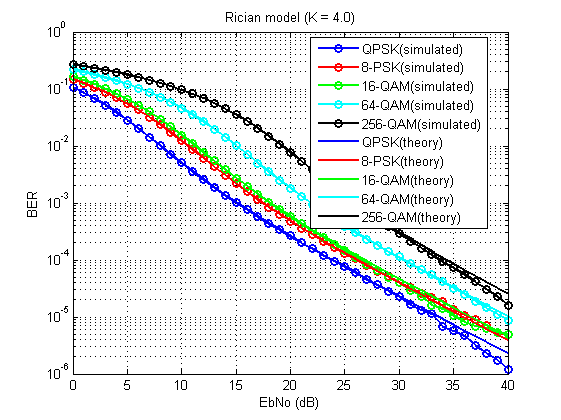\n",
268 | ">*Fig. 5. Bit error ratio performance of described ways of the modeling (K = 4.0).*\n",
269 | "\n",
270 | "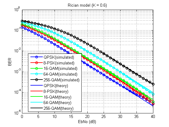\n",
271 | ">*Fig. 6. Bit error ratio performance of described ways of the modeling (K = 0.6).*\n",
272 | "\n",
273 | "As we can see in figures 5 and 6 BER performance of the proposal approaches completely matched with theoretical \\(**berfading\\(\\) function in MatLab**\\) results.\n"
274 | ]
275 | },
276 | {
277 | "cell_type": "markdown",
278 | "metadata": {},
279 | "source": [
280 | "# References\n",
281 | "\n",
282 | "1. Paulraj, Arogyaswami, Rohit Nabar, and Dhananjay Gore. Introduction to space-time wireless communications. Cambridge university press, 2003.\n",
283 | "\n",
284 | "2. Farrokhi, Farrokh R., et al. \"Spectral efficiency of FDMA/TDMA wireless systems with transmit and receive antenna arrays.\" IEEE transactions on wireless communications 1.4 (2002): 591-599.\n",
285 | "\n",
286 | "3. Goldsmith A. Wireless communications. – Cambridge university press, 2005.\n",
287 | "\n",
288 | "4. Fontæn, Fernando Pærez, and Perfecto Mariæo Espiæeira. Modelling the wireless propagation channel: a simulation approach with Matlab. Vol. 5. John Wiley & Sons, 2008.\n",
289 | "\n"
290 | ]
291 | },
292 | {
293 | "cell_type": "markdown",
294 | "metadata": {},
295 | "source": [
296 | "## Task solution\n",
297 | "\n",
298 | "\n",
299 | "$$ ||H_{LoS}||^2_F = \\sum^{M_R}_{i=1}\\sum^{M_T}_{j=1}|h^{(LoS)}_{ij}|^2 $$\n",
300 | "\n",
301 | "What is the $h^{(LoS)}_{ij}$? It is the **complex exponent** (e.g. $e^{j\\phi}$) anyway. Each complex exponent can be represented as the sum of the *cos* and *sin* components:\n",
302 | "\n",
303 | "$$ e^{j\\phi} = cos\\phi + jsin\\phi $$\n",
304 | "\n",
305 | "The squared absolute value of the complex value $z = x +jy$:\n",
306 | "\n",
307 | "$$ |z|^2 = x^2 + y^2 $$\n",
308 | "\n",
309 | "Hence:\n",
310 | "\n",
311 | "$$ |e^{j\\phi}|^2 = cos^2\\phi + sin^2\\phi = 1 $$\n",
312 | "\n",
313 | "And finally:\n",
314 | "\n",
315 | "$$ ||H_{LoS}||^2_F = M_RM_T $$\n"
316 | ]
317 | }
318 | ],
319 | "metadata": {
320 | "kernelspec": {
321 | "display_name": "Python 3",
322 | "language": "python",
323 | "name": "python3"
324 | },
325 | "language_info": {
326 | "codemirror_mode": {
327 | "name": "ipython",
328 | "version": 3
329 | },
330 | "file_extension": ".py",
331 | "mimetype": "text/x-python",
332 | "name": "python",
333 | "nbconvert_exporter": "python",
334 | "pygments_lexer": "ipython3",
335 | "version": "3.7.4"
336 | }
337 | },
338 | "nbformat": 4,
339 | "nbformat_minor": 2
340 | }
341 |
--------------------------------------------------------------------------------
"
252 | ]
253 | },
254 | {
255 | "cell_type": "markdown",
256 | "metadata": {},
257 | "source": [
258 | "> **Simulation script**:\n",
259 | ">\n",
260 | ">Vladimir Fadeev (2019). M-PSK and M-QAM over Rician flat fading channel (https://www.mathworks.com/matlabcentral/fileexchange/70559-m-psk-and-m-qam-over-rician-flat-fading-channel), MATLAB Central File Exchange. Retrieved October 7, 2019."
261 | ]
262 | },
263 | {
264 | "cell_type": "markdown",
265 | "metadata": {},
266 | "source": [
267 | "\n",
268 | ">*Fig. 5. Bit error ratio performance of described ways of the modeling (K = 4.0).*\n",
269 | "\n",
270 | "\n",
271 | ">*Fig. 6. Bit error ratio performance of described ways of the modeling (K = 0.6).*\n",
272 | "\n",
273 | "As we can see in figures 5 and 6 BER performance of the proposal approaches completely matched with theoretical \\(**berfading\\(\\) function in MatLab**\\) results.\n"
274 | ]
275 | },
276 | {
277 | "cell_type": "markdown",
278 | "metadata": {},
279 | "source": [
280 | "# References\n",
281 | "\n",
282 | "1. Paulraj, Arogyaswami, Rohit Nabar, and Dhananjay Gore. Introduction to space-time wireless communications. Cambridge university press, 2003.\n",
283 | "\n",
284 | "2. Farrokhi, Farrokh R., et al. \"Spectral efficiency of FDMA/TDMA wireless systems with transmit and receive antenna arrays.\" IEEE transactions on wireless communications 1.4 (2002): 591-599.\n",
285 | "\n",
286 | "3. Goldsmith A. Wireless communications. – Cambridge university press, 2005.\n",
287 | "\n",
288 | "4. Fontæn, Fernando Pærez, and Perfecto Mariæo Espiæeira. Modelling the wireless propagation channel: a simulation approach with Matlab. Vol. 5. John Wiley & Sons, 2008.\n",
289 | "\n"
290 | ]
291 | },
292 | {
293 | "cell_type": "markdown",
294 | "metadata": {},
295 | "source": [
296 | "## Task solution\n",
297 | "\n",
298 | "\n",
299 | "$$ ||H_{LoS}||^2_F = \\sum^{M_R}_{i=1}\\sum^{M_T}_{j=1}|h^{(LoS)}_{ij}|^2 $$\n",
300 | "\n",
301 | "What is the $h^{(LoS)}_{ij}$? It is the **complex exponent** (e.g. $e^{j\\phi}$) anyway. Each complex exponent can be represented as the sum of the *cos* and *sin* components:\n",
302 | "\n",
303 | "$$ e^{j\\phi} = cos\\phi + jsin\\phi $$\n",
304 | "\n",
305 | "The squared absolute value of the complex value $z = x +jy$:\n",
306 | "\n",
307 | "$$ |z|^2 = x^2 + y^2 $$\n",
308 | "\n",
309 | "Hence:\n",
310 | "\n",
311 | "$$ |e^{j\\phi}|^2 = cos^2\\phi + sin^2\\phi = 1 $$\n",
312 | "\n",
313 | "And finally:\n",
314 | "\n",
315 | "$$ ||H_{LoS}||^2_F = M_RM_T $$\n"
316 | ]
317 | }
318 | ],
319 | "metadata": {
320 | "kernelspec": {
321 | "display_name": "Python 3",
322 | "language": "python",
323 | "name": "python3"
324 | },
325 | "language_info": {
326 | "codemirror_mode": {
327 | "name": "ipython",
328 | "version": 3
329 | },
330 | "file_extension": ".py",
331 | "mimetype": "text/x-python",
332 | "name": "python",
333 | "nbconvert_exporter": "python",
334 | "pygments_lexer": "ipython3",
335 | "version": "3.7.4"
336 | }
337 | },
338 | "nbformat": 4,
339 | "nbformat_minor": 2
340 | }
341 |
--------------------------------------------------------------------------------