├── .gitignore
├── DataCamp_Model_Building.ipynb
├── Data_Camp_Exploration.ipynb
├── Python_intro_hackathon.sublime-project
├── Python_intro_hackathon.sublime-workspace
├── README.md
├── chapter1.md
├── chapter2.md
├── chapter3.md
├── chapter4.md
├── chapter5.md
├── chapter6.md
├── course.yml
├── img
├── author_image.png
└── shield_image.png
└── requirements.sh
/.gitignore:
--------------------------------------------------------------------------------
1 | .DS_STORE
2 | .cache
3 | .ipynb_checkpoints
4 | .spyderproject
5 |
--------------------------------------------------------------------------------
/DataCamp_Model_Building.ipynb:
--------------------------------------------------------------------------------
1 | {
2 | "cells": [
3 | {
4 | "cell_type": "markdown",
5 | "metadata": {},
6 | "source": [
7 | "# preprocessing of data set"
8 | ]
9 | },
10 | {
11 | "cell_type": "code",
12 | "execution_count": 3,
13 | "metadata": {
14 | "collapsed": true
15 | },
16 | "outputs": [],
17 | "source": [
18 | "import pandas as pd\n",
19 | "import numpy as np\n",
20 | "from sklearn.preprocessing import LabelEncoder\n",
21 | "\n",
22 | "train = pd.read_csv(\"https://s3-ap-southeast-1.amazonaws.com/av-datahack-datacamp/train.csv\")\n",
23 | "test = pd.read_csv(\"https://s3-ap-southeast-1.amazonaws.com/av-datahack-datacamp/test.csv\")"
24 | ]
25 | },
26 | {
27 | "cell_type": "code",
28 | "execution_count": 4,
29 | "metadata": {
30 | "collapsed": false
31 | },
32 | "outputs": [
33 | {
34 | "data": {
35 | "text/plain": [
36 | "ApplicantIncome 0\n",
37 | "CoapplicantIncome 0\n",
38 | "Credit_History 79\n",
39 | "Dependents 25\n",
40 | "Education 0\n",
41 | "Gender 24\n",
42 | "LoanAmount 27\n",
43 | "Loan_Amount_Term 20\n",
44 | "Loan_ID 0\n",
45 | "Loan_Status 367\n",
46 | "Married 3\n",
47 | "Property_Area 0\n",
48 | "Self_Employed 55\n",
49 | "Type 0\n",
50 | "dtype: int64"
51 | ]
52 | },
53 | "execution_count": 4,
54 | "metadata": {},
55 | "output_type": "execute_result"
56 | }
57 | ],
58 | "source": [
59 | "#Combining both train and test dataset\n",
60 | "\n",
61 | "train['Type']='Train' #Create a flag for Train and Test Data set\n",
62 | "test['Type']='Test'\n",
63 | "fullData = pd.concat([train,test],axis=0)\n",
64 | "\n",
65 | "#Look at the available missing values in the dataset\n",
66 | "fullData.isnull().sum()"
67 | ]
68 | },
69 | {
70 | "cell_type": "code",
71 | "execution_count": 5,
72 | "metadata": {
73 | "collapsed": true
74 | },
75 | "outputs": [],
76 | "source": [
77 | "#Identify categorical and continuous variables\n",
78 | "ID_col = ['Loan_ID']\n",
79 | "target_col = [\"Loan_Status\"]\n",
80 | "cat_cols = ['Credit_History','Dependents','Gender','Married','Education','Property_Area','Self_Employed']\n",
81 | "\n",
82 | "other_col=['Type'] #Test and Train Data set identifier\n",
83 | "num_cols= list(set(list(fullData.columns))-set(cat_cols)-set(ID_col)-set(target_col)-set(other_col))"
84 | ]
85 | },
86 | {
87 | "cell_type": "code",
88 | "execution_count": 6,
89 | "metadata": {
90 | "collapsed": false
91 | },
92 | "outputs": [
93 | {
94 | "name": "stderr",
95 | "output_type": "stream",
96 | "text": [
97 | "C:\\Users\\abc\\Anaconda2\\lib\\site-packages\\pandas\\core\\generic.py:3178: SettingWithCopyWarning: \n",
98 | "A value is trying to be set on a copy of a slice from a DataFrame\n",
99 | "\n",
100 | "See the caveats in the documentation: http://pandas.pydata.org/pandas-docs/stable/indexing.html#indexing-view-versus-copy\n",
101 | " self._update_inplace(new_data)\n"
102 | ]
103 | }
104 | ],
105 | "source": [
106 | "#Imputing Missing values with mean for continuous variable\n",
107 | "fullData[num_cols] = fullData[num_cols].fillna(fullData[num_cols].mean(),inplace=True)\n",
108 | "\n",
109 | "\n",
110 | "#Imputing Missing values with mode for categorical variables\n",
111 | "cat_imput=pd.Series(fullData[cat_cols].mode().values[0])\n",
112 | "cat_imput.index=cat_cols\n",
113 | "fullData[cat_cols] = fullData[cat_cols].fillna(cat_imput,inplace=True)"
114 | ]
115 | },
116 | {
117 | "cell_type": "code",
118 | "execution_count": 7,
119 | "metadata": {
120 | "collapsed": true
121 | },
122 | "outputs": [],
123 | "source": [
124 | "#Create a new column as Total Income\n",
125 | "\n",
126 | "fullData['TotalIncome']=fullData['ApplicantIncome']+fullData['CoapplicantIncome']\n",
127 | "\n",
128 | "#Take a log of TotalIncome + 1, adding 1 to deal with zeros of TotalIncome it it exists\n",
129 | "fullData['Log_TotalIncome']=np.log(fullData['TotalIncome'])\n"
130 | ]
131 | },
132 | {
133 | "cell_type": "code",
134 | "execution_count": 8,
135 | "metadata": {
136 | "collapsed": false
137 | },
138 | "outputs": [
139 | {
140 | "name": "stderr",
141 | "output_type": "stream",
142 | "text": [
143 | "C:\\Users\\abc\\Anaconda2\\lib\\site-packages\\ipykernel\\__main__.py:8: SettingWithCopyWarning: \n",
144 | "A value is trying to be set on a copy of a slice from a DataFrame.\n",
145 | "Try using .loc[row_indexer,col_indexer] = value instead\n",
146 | "\n",
147 | "See the caveats in the documentation: http://pandas.pydata.org/pandas-docs/stable/indexing.html#indexing-view-versus-copy\n"
148 | ]
149 | }
150 | ],
151 | "source": [
152 | "#create label encoders for categorical features\n",
153 | "for var in cat_cols:\n",
154 | " number = LabelEncoder()\n",
155 | " fullData[var] = number.fit_transform(fullData[var].astype('str'))\n",
156 | "\n",
157 | "train_modified=fullData[fullData['Type']=='Train']\n",
158 | "test_modified=fullData[fullData['Type']=='Test']\n",
159 | "train_modified[\"Loan_Status\"] = number.fit_transform(train_modified[\"Loan_Status\"].astype('str'))"
160 | ]
161 | },
162 | {
163 | "cell_type": "markdown",
164 | "metadata": {},
165 | "source": [
166 | "# Building Logistic Regression"
167 | ]
168 | },
169 | {
170 | "cell_type": "code",
171 | "execution_count": 9,
172 | "metadata": {
173 | "collapsed": false
174 | },
175 | "outputs": [],
176 | "source": [
177 | "from sklearn.linear_model import LogisticRegression\n",
178 | "\n",
179 | "\n",
180 | "predictors=['Credit_History','Education','Gender']\n",
181 | "\n",
182 | "x_train = train_modified[list(predictors)].values\n",
183 | "y_train = train_modified[\"Loan_Status\"].values\n",
184 | "\n",
185 | "x_test=test_modified[list(predictors)].values"
186 | ]
187 | },
188 | {
189 | "cell_type": "code",
190 | "execution_count": 10,
191 | "metadata": {
192 | "collapsed": false
193 | },
194 | "outputs": [
195 | {
196 | "name": "stderr",
197 | "output_type": "stream",
198 | "text": [
199 | "C:\\Users\\abc\\Anaconda2\\lib\\site-packages\\ipykernel\\__main__.py:14: SettingWithCopyWarning: \n",
200 | "A value is trying to be set on a copy of a slice from a DataFrame.\n",
201 | "Try using .loc[row_indexer,col_indexer] = value instead\n",
202 | "\n",
203 | "See the caveats in the documentation: http://pandas.pydata.org/pandas-docs/stable/indexing.html#indexing-view-versus-copy\n"
204 | ]
205 | }
206 | ],
207 | "source": [
208 | "# Create logistic regression object\n",
209 | "model = LogisticRegression()\n",
210 | "\n",
211 | "# Train the model using the training sets\n",
212 | "model.fit(x_train, y_train)\n",
213 | "\n",
214 | "#Predict Output\n",
215 | "predicted= model.predict(x_test)\n",
216 | "\n",
217 | "#Reverse encoding for predicted outcome\n",
218 | "predicted = number.inverse_transform(predicted)\n",
219 | "\n",
220 | "#Store it to test dataset\n",
221 | "test_modified['Loan_Status']=predicted\n",
222 | "\n",
223 | "#Output file to make submission\n",
224 | "test_modified.to_csv(\"Submission1.csv\",columns=['Loan_ID','Loan_Status'])"
225 | ]
226 | },
227 | {
228 | "cell_type": "markdown",
229 | "metadata": {},
230 | "source": [
231 | "# Building Decision Tree Classifier"
232 | ]
233 | },
234 | {
235 | "cell_type": "code",
236 | "execution_count": 11,
237 | "metadata": {
238 | "collapsed": true
239 | },
240 | "outputs": [],
241 | "source": [
242 | "predictors=['Credit_History','Education','Gender']\n",
243 | "\n",
244 | "x_train = train_modified[list(predictors)].values\n",
245 | "y_train = train_modified[\"Loan_Status\"].values\n",
246 | "\n",
247 | "x_test=test_modified[list(predictors)].values"
248 | ]
249 | },
250 | {
251 | "cell_type": "code",
252 | "execution_count": 12,
253 | "metadata": {
254 | "collapsed": false
255 | },
256 | "outputs": [
257 | {
258 | "name": "stderr",
259 | "output_type": "stream",
260 | "text": [
261 | "C:\\Users\\abc\\Anaconda2\\lib\\site-packages\\ipykernel\\__main__.py:16: SettingWithCopyWarning: \n",
262 | "A value is trying to be set on a copy of a slice from a DataFrame.\n",
263 | "Try using .loc[row_indexer,col_indexer] = value instead\n",
264 | "\n",
265 | "See the caveats in the documentation: http://pandas.pydata.org/pandas-docs/stable/indexing.html#indexing-view-versus-copy\n"
266 | ]
267 | }
268 | ],
269 | "source": [
270 | "from sklearn.tree import DecisionTreeClassifier\n",
271 | "\n",
272 | "# Create Decision Tree object\n",
273 | "model = DecisionTreeClassifier()\n",
274 | "\n",
275 | "# Train the model using the training sets\n",
276 | "model.fit(x_train, y_train)\n",
277 | "\n",
278 | "#Predict Output\n",
279 | "predicted= model.predict(x_test)\n",
280 | "\n",
281 | "#Reverse encoding for predicted outcome\n",
282 | "predicted = number.inverse_transform(predicted)\n",
283 | "\n",
284 | "#Store it to test dataset\n",
285 | "test_modified['Loan_Status']=predicted\n",
286 | "\n",
287 | "#Output file to make submission\n",
288 | "test_modified.to_csv(\"Submission2.csv\",columns=['Loan_ID','Loan_Status'])\n"
289 | ]
290 | },
291 | {
292 | "cell_type": "markdown",
293 | "metadata": {},
294 | "source": [
295 | "# Building Random Forest Classifier"
296 | ]
297 | },
298 | {
299 | "cell_type": "code",
300 | "execution_count": 13,
301 | "metadata": {
302 | "collapsed": true
303 | },
304 | "outputs": [],
305 | "source": [
306 | "from sklearn.linear_model import LogisticRegression\n",
307 | "\n",
308 | "\n",
309 | "predictors=['ApplicantIncome', 'CoapplicantIncome', 'Credit_History','Dependents', 'Education', 'Gender', 'LoanAmount',\n",
310 | " 'Loan_Amount_Term', 'Married', 'Property_Area', 'Self_Employed', 'TotalIncome','Log_TotalIncome']\n",
311 | "\n",
312 | "x_train = train_modified[list(predictors)].values\n",
313 | "y_train = train_modified[\"Loan_Status\"].values\n",
314 | "\n",
315 | "x_test=test_modified[list(predictors)].values"
316 | ]
317 | },
318 | {
319 | "cell_type": "code",
320 | "execution_count": 14,
321 | "metadata": {
322 | "collapsed": false
323 | },
324 | "outputs": [
325 | {
326 | "name": "stderr",
327 | "output_type": "stream",
328 | "text": [
329 | "C:\\Users\\abc\\Anaconda2\\lib\\site-packages\\ipykernel\\__main__.py:16: SettingWithCopyWarning: \n",
330 | "A value is trying to be set on a copy of a slice from a DataFrame.\n",
331 | "Try using .loc[row_indexer,col_indexer] = value instead\n",
332 | "\n",
333 | "See the caveats in the documentation: http://pandas.pydata.org/pandas-docs/stable/indexing.html#indexing-view-versus-copy\n"
334 | ]
335 | }
336 | ],
337 | "source": [
338 | "from sklearn.ensemble import RandomForestClassifier\n",
339 | "\n",
340 | "# Create Decision Tree object\n",
341 | "model = RandomForestClassifier()\n",
342 | "\n",
343 | "# Train the model using the training sets\n",
344 | "model.fit(x_train, y_train)\n",
345 | "\n",
346 | "#Predict Output\n",
347 | "predicted= model.predict(x_test)\n",
348 | "\n",
349 | "#Reverse encoding for predicted outcome\n",
350 | "predicted = number.inverse_transform(predicted)\n",
351 | "\n",
352 | "#Store it to test dataset\n",
353 | "test_modified['Loan_Status']=predicted\n",
354 | "\n",
355 | "#Output file to make submission\n",
356 | "test_modified.to_csv(\"Submission3.csv\",columns=['Loan_ID','Loan_Status'])\n"
357 | ]
358 | },
359 | {
360 | "cell_type": "code",
361 | "execution_count": 15,
362 | "metadata": {
363 | "collapsed": false
364 | },
365 | "outputs": [
366 | {
367 | "name": "stdout",
368 | "output_type": "stream",
369 | "text": [
370 | "Credit_History 0.232724\n",
371 | "TotalIncome 0.146955\n",
372 | "LoanAmount 0.128687\n",
373 | "ApplicantIncome 0.114424\n",
374 | "Log_TotalIncome 0.113866\n",
375 | "CoapplicantIncome 0.082272\n",
376 | "Dependents 0.038125\n",
377 | "Property_Area 0.036118\n",
378 | "Loan_Amount_Term 0.032650\n",
379 | "Married 0.022713\n",
380 | "Self_Employed 0.022481\n",
381 | "Education 0.016459\n",
382 | "Gender 0.012527\n",
383 | "dtype: float64\n"
384 | ]
385 | }
386 | ],
387 | "source": [
388 | "#Create a series with feature importances:\n",
389 | "featimp = pd.Series(model.feature_importances_, index=predictors).sort_values(ascending=False)\n",
390 | "print featimp"
391 | ]
392 | },
393 | {
394 | "cell_type": "code",
395 | "execution_count": 16,
396 | "metadata": {
397 | "collapsed": true
398 | },
399 | "outputs": [],
400 | "source": [
401 | "number = LabelEncoder()\n",
402 | "train['Gender'] = number.fit_transform(train['Gender'].astype('str'))\n",
403 | " "
404 | ]
405 | },
406 | {
407 | "cell_type": "code",
408 | "execution_count": 17,
409 | "metadata": {
410 | "collapsed": false
411 | },
412 | "outputs": [
413 | {
414 | "data": {
415 | "text/plain": [
416 | "0 1\n",
417 | "1 1\n",
418 | "2 1\n",
419 | "3 1\n",
420 | "4 1\n",
421 | "5 1\n",
422 | "6 1\n",
423 | "7 1\n",
424 | "8 1\n",
425 | "9 1\n",
426 | "10 1\n",
427 | "11 1\n",
428 | "12 1\n",
429 | "13 1\n",
430 | "14 1\n",
431 | "15 1\n",
432 | "16 1\n",
433 | "17 0\n",
434 | "18 1\n",
435 | "19 1\n",
436 | "20 1\n",
437 | "21 1\n",
438 | "22 1\n",
439 | "23 2\n",
440 | "24 1\n",
441 | "25 1\n",
442 | "26 1\n",
443 | "27 1\n",
444 | "28 1\n",
445 | "29 0\n",
446 | " ..\n",
447 | "584 1\n",
448 | "585 1\n",
449 | "586 1\n",
450 | "587 0\n",
451 | "588 2\n",
452 | "589 1\n",
453 | "590 1\n",
454 | "591 1\n",
455 | "592 2\n",
456 | "593 1\n",
457 | "594 1\n",
458 | "595 1\n",
459 | "596 1\n",
460 | "597 1\n",
461 | "598 1\n",
462 | "599 1\n",
463 | "600 0\n",
464 | "601 1\n",
465 | "602 1\n",
466 | "603 1\n",
467 | "604 0\n",
468 | "605 1\n",
469 | "606 1\n",
470 | "607 1\n",
471 | "608 1\n",
472 | "609 0\n",
473 | "610 1\n",
474 | "611 1\n",
475 | "612 1\n",
476 | "613 0\n",
477 | "Name: Gender, dtype: int64"
478 | ]
479 | },
480 | "execution_count": 17,
481 | "metadata": {},
482 | "output_type": "execute_result"
483 | }
484 | ],
485 | "source": [
486 | "train.Gender"
487 | ]
488 | },
489 | {
490 | "cell_type": "code",
491 | "execution_count": null,
492 | "metadata": {
493 | "collapsed": true
494 | },
495 | "outputs": [],
496 | "source": []
497 | }
498 | ],
499 | "metadata": {
500 | "kernelspec": {
501 | "display_name": "Python 2",
502 | "language": "python",
503 | "name": "python2"
504 | },
505 | "language_info": {
506 | "codemirror_mode": {
507 | "name": "ipython",
508 | "version": 2
509 | },
510 | "file_extension": ".py",
511 | "mimetype": "text/x-python",
512 | "name": "python",
513 | "nbconvert_exporter": "python",
514 | "pygments_lexer": "ipython2",
515 | "version": "2.7.11"
516 | }
517 | },
518 | "nbformat": 4,
519 | "nbformat_minor": 0
520 | }
521 |
--------------------------------------------------------------------------------
/Python_intro_hackathon.sublime-project:
--------------------------------------------------------------------------------
1 | {
2 | "folders":
3 | [
4 | {
5 | "path": "."
6 | }
7 | ]
8 | }
9 |
--------------------------------------------------------------------------------
/Python_intro_hackathon.sublime-workspace:
--------------------------------------------------------------------------------
1 | {
2 | "auto_complete":
3 | {
4 | "selected_items":
5 | [
6 | [
7 | "text",
8 | "text_size_change"
9 | ],
10 | [
11 | "get",
12 | "getElementById"
13 | ],
14 | [
15 | "butt",
16 | "button_text_to_change"
17 | ],
18 | [
19 | "button",
20 | "button1"
21 | ],
22 | [
23 | "m",
24 | "myImage"
25 | ],
26 | [
27 | "on",
28 | "onclick Attr"
29 | ],
30 | [
31 | "name",
32 | "name"
33 | ],
34 | [
35 | "format",
36 | "formattedRole"
37 | ],
38 | [
39 | "formatted",
40 | "formattedName"
41 | ],
42 | [
43 | "fun",
44 | "funThoughts"
45 | ],
46 | [
47 | "For",
48 | "ForeignKey"
49 | ],
50 | [
51 | "resta",
52 | "restaurant"
53 | ],
54 | [
55 | "nu",
56 | "nullable"
57 | ],
58 | [
59 | "cre",
60 | "create_engine"
61 | ],
62 | [
63 | "dec",
64 | "declarative_base"
65 | ]
66 | ]
67 | },
68 | "buffers":
69 | [
70 | {
71 | "contents": "\ntitle : Python Libraries and data structures\ndescription : In this chapter, we will take you through the libraries we commonly use in data analysis and introduce some of the most common data structures to you.\nattachments :\n slides_link : https://s3.amazonaws.com/assets.datacamp.com/course/teach/slides_example.pdf\n\n--- type:NormalExercise lang:python xp:100 skills:1 key:af2f6f90f3\n## Create a list\n\nList is one of the most versatile data structure in Python. A list can simply be defined by writing a list of comma separated values in square brackets. Lists might contain items of different types. Python lists are mutable and individual elements of a list can be changed.\n\n```{python}\nCountry =['INDIA','USA','GERMANY','UK','AUSTRALIA']\n\nTemperature =[44, 28, 20, 18, 25, 45, 67]\n```\nWe just created two lists, one for Country names and other one for temperature. \n\n####Accessing individual elements of a list\n- Individual elements of a list can be accessed by writting an index number in square bracket. First index of list starts with 0 (zero) not 1.\n- A range of element can be accessed by having start index and end index but it does not return the value available at end index,\n\n*** =instructions\n- Create a list of first five odd numbers and store it in a variable odd_numbers.\n- Print second to fourth element [1, 4, 9] from squares_lis,t\n\n\n*** =hint\n- Use AV[0] to select the first element of a list AV. \n- Use AV[1:3] to select second to third element of a list AV.\n\n\n*** =pre_exercise_code\n```{python}\n# The pre exercise code runs code to initialize the user's workspace. You can use it for several things:\n```\n\n*** =sample_code\n\n```{python}\n\n# Create a list of squared numbers\nsquares_list = [0, 1, 4, 9, 16, 25]\n\n# Now write a code to create list of first five odd numbers and store it into a variable odd_numbers\nodd_numbers=\n\n# Print first element of squares_list\nprint (squares_list[0])\n\n# Print second to fourth elements of squares_list\n\n```\n\n*** =solution\n```{python}\n\n# Create a list of squared numbers\nsquares_list = [0, 1, 4, 9, 16, 25]\n\n# Now write a code to create list of first five odd numbers and store it into a variable odd_numbers\nodd_numbers = [1, 3, 5, 7, 9]\n\n# Print first element of squares_list\nprint (squares_list[0])\n\n# Print second to fourth elements of squares_list\nprint (squares_list[1:4])\n```\n\n*** =sct\n```{python}\n# The sct section defines the Submission Correctness Tests (SCTs) used to\n# evaluate the student's response. All functions used here are defined in the \n# pythonwhat Python package. Documentation can also be found at github.com/datacamp/pythonwhat/wiki\n\n# Test for list of odd_numbers\ntest_object(\"odd_numbers\")\n\n# Check second to fourth elements\"\ntest_output_contains(\"[1, 4, 9]\", pattern = False)\nsuccess_msg(\"Great work!\")\n```\n\n--- type:NormalExercise lang:python xp:100 skills:1 key:c7f91e389f\n## Create a String\n\nStrings can simply be defined by use of single ( ‘ ), double ( ” ) or triple ( ”’ ) inverted commas. Strings enclosed in triple quotes ( ”’ ) can span over multiple lines. Please note that Python strings are immutable, so you can not change part of strings.\n\n```{python}\nString =\" Strings elements can also be accessed using index number like list\"\n\nprint (String[0:8])\n\n#Above print command display Strings on screen.\n\n```\n\n\n*** =instructions\n\n- len function returns the lenght of string\n- Strings characters can be accessed using index number (similar like list)\n- Strings can be concatenated with other strings using '+' operator\n\n\n\n*** =hint\n\n- Use str[2] to select the third element of string str \n- Use len(str) to return the length of string\n- Use str1 + str2 to return the concatenated result of both strings str1 and str2\n\n\n\n*** =pre_exercise_code\n\n```{python}\n# The pre exercise code runs code to initialize the user's workspace. You can use it for several things:\n```\n\n*** =sample_code\n\n```{python}\n# Create a string str\nstr1 = \"Introduction with strings\"\n\n# Now store the length of string in varible str_len \nstr_len =\n\n# Print last seven characters of strings str\n\n\nstr1 = \"I am doing a course Introduction to Hackathon using \"\nstr2 = \"Python\"\n\n# Write a code to store concatenated string of str1 and str2 into variable str3\nstr3 =\n\n```\n\n*** =solution\n\n```{python}\n\n# Create a string str\nstr1 = \"Introduction with strings\"\n\n# Now store the length of string in varible str_len \nstr_len=len(str1)\n\n# Print last seven characters of strings str\nprint (str1[18:25])\n\nstr1 = \"I am doing a course Introduction to Hackathon using \"\nstr2 = \"Python\"\n\n# Write a code to store concatenated string of str1 and str2 into variable str3\nstr3= str1 + str2\n```\n\n*** =sct\n\n```{python}\n# The sct section defines the Submission Correctness Tests (SCTs) used to\n# evaluate the student's response. All functions used here are defined in the \n# pythonwhat Python package. Documentation can also be found at github.com/datacamp/pythonwhat/wiki\n\n# Check length of strings\ntest_object(\"str_len\")\n\n# Check last seven characters\ntest_output_contains(\"strings\", pattern = False)\n\n# Check concatenated strings\"\ntest_object(\"str3\")\nsuccess_msg(\"Great work!\")\n```\n\n--- type:NormalExercise lang:python xp:100 skills:1 key:377e9324f2\n## Create a Dictionary\n\nDictionary is an unordered set of key: value pairs, with the requirement that the keys are unique (within one dictionary). A pair of braces creates an empty dictionary: {}.\n\n```{python}\nDICT = {'Name':'Kunal', 'Company':'Analytics Vidhya'}\n\n#Dictionary elements can be accessed by \"keys\"\n\nprint (DICT['Name'])\n\n#Above print statement will print Kunal\n\n```\n\nIn dictonary \"DICT\", Name and Company are dictionary keys where as \"Kunal\" and \"Analytics Vidhya\" are values.\n\n*** =instructions\n\n- To access dictionary elements, you can use the familiar square brackets along with the key to obtain its value\n- Dictionary can be updated by adding a new entry or a key-value pair, modifying or deleting an existing entry\n\n*** =hint\n\n- Use dict['Keys'] = new_value to update the existing value\n- Use dict.keys() to access all keys of dictionary dict\n- Use dict.values() to access all values of dictionary dict\n\n\n*** =pre_exercise_code\n\n```{python}\n# The pre exercise code runs code to initialize the user's workspace. You can use it for several things:\n```\n\n*** =sample_code\n\n```{python}\n\n# Create a dictionary\ndict1 = {'Name': 'Max', 'Age': 16, 'Sports': 'Cricket'}\n\n# Update the value of Age to 18\n\n\n# Print the value of Age\n\n\n# Print all the keys of dictionary dict1\n\n\n```\n\n*** =solution\n\n```{python}\n\n# Create a dictionary\ndict1 = {'Name': 'Max', 'Age': 16, 'Sports': 'Cricket'}\n\n# Update the value of Age to 18\ndict1['Age'] = 18\n\n# Print the value of Age\nprint (dict1['Age'])\n\n# Print all the keys of dictionary dict\nprint (dict1.keys())\n\n```\n\n*** =sct\n\n```{python}\n# The sct section defines the Submission Correctness Tests (SCTs) used to\n# evaluate the student's response. All functions used here are defined in the \n# pythonwhat Python package. Documentation can also be found at github.com/datacamp/pythonwhat/wiki\n\n# Check value of Age\ntest_output_contains(\"18\", pattern = False)\n\n# Check keys of dictionary\ntest_output_contains(\"dict_keys(['Name', 'Age', 'Sports'])\", pattern = False)\n\nsuccess_msg(\"Great work!\")\n```\n\n--- type:MultipleChoiceExercise lang:python xp:50 skills:1 key:9a8fd577a9\n## Why python libraries are useful?\n\nLets take one step ahead in our journey to learn Python by getting acquainted with some useful libraries. The first step is obviously to learn to import them into our environment. There are several ways of doing so in Python:\n\n```{python}\nimport math as m\n\nfrom math import *\n```\n\nIn the first manner, we have defined an alias m to library math. We can now use various functions from math library (e.g. factorial) by referencing it using the alias m.factorial().\n\nIn the second manner, you have imported the entire name space in math i.e. you can directly use factorial() without referring to math.\n\nFollowing are a list of libraries, you will need for any scientific computations and data analysis:\n\n* Numpy \n* Scipy \n* Pandas \n* Matplotlib \n* Scikit Learn \n\n\n\n##### Which of the following is a valid import statement for below code?\n```{python}\nprint (factorial(5))\n```\n\n*** =instructions\n- import math\n- from math import factorial\n- import math.factorial\n\n*** =hint\nPython's from statement lets you import specific attributes from a module into the current namespace.\n\n*** =pre_exercise_code\n\n\n*** =sct\n```{python}\n# The sct section defines the Submission Correctness Tests (SCTs) used to\n# evaluate the student's response. All functions used here are defined in the \n# pythonwhat Python package\n\nmsg_bad = \"Read about importing libraries in python\"\nmsg_success = \"Good Job!\"\n\n# Use test_mc() to grade multiple choice exercises. \n# Pass the correct option (Action, option 2 in the instructions) to correct.\n# Pass the feedback messages, both positive and negative, to feedback_msgs in the appropriate order.\ntest_mc(2, [msg_bad, msg_success, msg_bad]) \n```\n\n\n--- type:NormalExercise lang:python xp:100 skills:1 key:50c9218dac\n## Why conditional statement is required?\n\nConditional statements, these are used to execute code fragments based on a condition. The most commonly used construct is if-else, with following syntax:\n\n```{python}\n\nif [condition]:\n __execution if true__\nelse:\n __execution if false__ \n```\n\n*** =instructions\n\n- Store the length of squares_list to square_len\n- Use the if statement to perform one action if one thing is true,or any other actions, if something else is true\n\n\n*** =hint\n\n- Use <, >, <=, >=, == and != for comparison\n- Use len(list) to return length of string\n\n\n*** =pre_exercise_code\n\n```{python}\n# The pre exercise code runs code to initialize the user's workspace. You can use it for several things:\n```\n\n*** =sample_code\n\n```{python}\n# Create a two integer variables a and b\na=3\nb=4\n\n# if a is greater than b print a-b else a+b\nif a > b:\n print (a-b)\nelse:\n print (a+b)\n\n# Create a list of squared numbers\nsquares_list = [0, 1, 4, 9, 16, 25]\n\n# Store the length of squares_list in square_len\nsquare_len = \n\n# if square_len is less than 5 then print \"Less than 5\" else \"Greater than 5\"\nif square_len < ___:\n print (\"__________\")\nelse:\n print (\"__________\")\n\n\n```\n\n*** =solution\n\n```{python}\n# Create a two integer variables a and b\na=3\nb=4\n\n# if a is greater than b print a-b else a+b\nif a > b:\n print (a-b)\nelse:\n print (a+b)\n\n# Create a list of squared numbers\nsquares_list = [0, 1, 4, 9, 16, 25]\n\n# Store the length of squares_list in square_len\nsquare_len = len(squares_list)\n\n# if square_len is less than 5 then print \"Less than 5\" else \"Greater than 5\"\nif square_len < 5:\n print (\"Less than 5\")\nelse:\n print (\"Greater than 5\")\n\n```\n\n*** =sct\n\n```{python}\n# The sct section defines the Submission Correctness Tests (SCTs) used to\n# evaluate the student's response. All functions used here are defined in the \n# pythonwhat Python package. Documentation can also be found at github.com/datacamp/pythonwhat/wiki\n\n# Check length of strings\ntest_object(\"square_len\")\n\n# Check last seven characters\ntest_output_contains(\"Greater than 5\", pattern = False)\n\nsuccess_msg(\"Great work!\")\n```\n\n\n--- type:NormalExercise lang:python xp:100 skills:1 key:c1b7c2fd5c\n## How iterative statement does help?\n\nComputers are often used to automate repetitive tasks. Repeating identical or similar tasks without making errors is something that computers do well. Repeated execution of a set of statements is called iteration.\n\nLike most languages, Python also has a FOR-loop which is the most widely used method for iteration. It has a simple syntax:\n\n```{python}\n\nfor i in [Python Iterable]:\n expression(i)\n\n```\n“Python Iterable” can be a list or other advanced data structures which we will explore in later sections. Let’s take a look at a simple example, determining the factorial of a number.\n\n*** =instructions\n\n- Use list.append() to append values in a list\n- Iterate over list to access each element of list\n\n\n\n*** =hint\n\n- Use <, >, <=, >=, == and != for comparison\n- Use len(list) to return length of string\n- % operator helps to return remainder e.g. 4 % 3 would be 1\n\n*** =pre_exercise_code\n\n```{python}\n# The pre exercise code runs code to initialize the user's workspace. You can use it for several things:\n```\n\n*** =sample_code\n\n```{python}\n# Create a list with first five numbers\nls=[]\nfor x in range(5):\n ls.append(x)\n \nsum=0\n# Store sum all even numbers of the list ls in sum\n\nfor x in ls: \n if ______: \n sum += x\n\n```\n\n*** =solution\n\n```{python}\n# Create a list with first five numbers\nls=[]\nfor x in range(5):\n ls.append(x) # append a value to a list\n \nsum=0\n# Store sum all even numbers of the list ls in sum\n\nfor x in ls: \n if x%2==0: \n sum += x\n\n```\n\n*** =sct\n\n```{python}\n# The sct section defines the Submission Correctness Tests (SCTs) used to\n# evaluate the student's response. All functions used here are defined in the \n# pythonwhat Python package. Documentation can also be found at github.com/datacamp/pythonwhat/wiki\n\n# Check length of strings\ntest_object(\"sum\")\n\nsuccess_msg(\"Great work!\")\n```\n",
72 | "file": "chapter2.md",
73 | "file_size": 13909,
74 | "file_write_time": 131096300693332037,
75 | "settings":
76 | {
77 | "buffer_size": 13384,
78 | "line_ending": "Windows"
79 | }
80 | },
81 | {
82 | "contents": "Analytics Vidhya\nAbout Us\nTeam\nCareers\n\n\nFor Data Scientists\nBlog\nDiscussions\nHackathons\nJobs\n",
83 | "settings":
84 | {
85 | "buffer_size": 94,
86 | "line_ending": "Windows",
87 | "name": "Analytics Vidhya"
88 | }
89 | },
90 | {
91 | "file": "chapter7.md",
92 | "settings":
93 | {
94 | "buffer_size": 7564,
95 | "line_ending": "Windows"
96 | }
97 | },
98 | {
99 | "contents": "---\ntitle : Tips and Tricks from the best hackers!\ndescription : Here is the best part of a hackathon - you learn from the best hackers as you compete against them. This chapter just brings out some tips and tricks as shared by the best hackers.\nattachments :\n slides_link : https://s3.amazonaws.com/assets.datacamp.com/course/teach/slides_example.pdf\n\n--- type:VideoExercise lang:python xp:50 skills:1 key:c55198c91d\n## Analyze movie ratings\n\n*** =video_link\n//player.vimeo.com/video/154783078\n\n--- type:MultipleChoiceExercise lang:python xp:50 skills:1 key:9a8fd577a9\n## A really bad movie\n\nHave a look at the plot that showed up in the viewer to the right. Which type of movies have the worst rating assigned to them?\n\n*** =instructions\n- Long movies, clearly\n- Short movies, clearly\n- Long movies, but the correlation seems weak\n- Short movies, but the correlation seems weak\n\n*** =hint\nHave a look at the plot. Do you see a trend in the dots?\n\n*** =pre_exercise_code\n```{r}\n# The pre exercise code runs code to initialize the user's workspace. You can use it for several things:\n\n# 1. Pre-load packages, so that users don't have to do this manually.\nimport pandas as pd\nimport matplotlib.pyplot as plt\n\n# 2. Preload a dataset. The code below will read the csv that is stored at the URL's location.\n# The movies variable will be available in the user's console.\nmovies = pd.read_csv(\"http://s3.amazonaws.com/assets.datacamp.com/course/introduction_to_r/movies.csv\")\n\n# 3. Create a plot in the viewer, that students can check out while reading the exercise\nplt.scatter(movies.runtime, movies.rating)\nplt.show()\n```\n\n*** =sct\n```{r}\n# The sct section defines the Submission Correctness Tests (SCTs) used to\n# evaluate the student's response. All functions used here are defined in the \n# pythonwhat Python package\n\nmsg_bad = \"That is not correct!\"\nmsg_success = \"Exactly! The correlation is very weak though.\"\n\n# Use test_mc() to grade multiple choice exercises. \n# Pass the correct option (Action, option 2 in the instructions) to correct.\n# Pass the feedback messages, both positive and negative, to feedback_msgs in the appropriate order.\ntest_mc(4, [msg_bad, msg_bad, msg_bad, msg_success]) \n```\n\n--- type:MultipleChoiceExercise lang:python xp:50 skills:1 key:f0e6a8e8a5\n## A really bad movie\n\nHave a look at the plot that showed up in the viewer to the right. Which type of movies have the worst rating assigned to them?\n\n*** =instructions\n- Long movies, clearly\n- Short movies, clearly\n- Long movies, but the correlation seems weak\n- Short movies, but the correlation seems weak\n\n*** =hint\nHave a look at the plot. Do you see a trend in the dots?\n\n*** =pre_exercise_code\n```{python}\n# The pre exercise code runs code to initialize the user's workspace. You can use it for several things:\n\n# 1. Pre-load packages, so that users don't have to do this manually.\nimport pandas as pd\nimport matplotlib.pyplot as plt\n\n# 2. Preload a dataset. The code below will read the csv that is stored at the URL's location.\n# The movies variable will be available in the user's console.\nmovies = pd.read_csv(\"http://s3.amazonaws.com/assets.datacamp.com/course/introduction_to_r/movies.csv\")\n\n# 3. Create a plot in the viewer, that students can check out while reading the exercise\nplt.scatter(movies.runtime, movies.rating)\nplt.show()\n```\n\n*** =sct\n```{python}\n# The sct section defines the Submission Correctness Tests (SCTs) used to\n# evaluate the student's response. All functions used here are defined in the\n# pythonwhat Python package\n\nmsg_bad = \"That is not correct!\"\nmsg_success = \"Exactly! The correlation is very weak though.\"\n\n# Use test_mc() to grade multiple choice exercises.\n# Pass the correct option (option 4 in the instructions) to correct.\n# Pass the feedback messages, both positive and negative, to feedback_msgs in the appropriate order.\ntest_mc(4, [msg_bad, msg_bad, msg_bad, msg_success])\n```\n\n--- type:NormalExercise lang:python xp:100 skills:1 key:af2f6f90f3\n## Plot the movies yourself\n\nDo you remember the plot of the last exercise? Let's make an even cooler plot!\n\nA dataset of movies, `movies`, is available in the workspace.\n\n*** =instructions\n- The first function, `np.unique()`, uses the `unique()` function of the `numpy` package to get integer values for the movie genres. You don't have to change this code, just have a look!\n- Import `pyplot` in the `matplotlib` package. Set an alias for this import: `plt`.\n- Use `plt.scatter()` to plot `movies.runtime` onto the x-axis, `movies.rating` onto the y-axis and use `ints` for the color of the dots. You should use the first and second positional argument, and the `c` keyword.\n- Show the plot using `plt.show()`.\n\n*** =hint\n- You don't have to program anything for the first instruction, just take a look at the first line of code.\n- Use `import ___ as ___` to import `matplotlib.pyplot` as `plt`.\n- Use `plt.scatter(___, ___, c = ___)` for the third instruction.\n- You'll always have to type in `plt.show()` to show the plot you created.\n\n*** =pre_exercise_code\n```{python}\n# The pre exercise code runs code to initialize the user's workspace. You can use it for several things:\n\n# 1. Preload a dataset. The code below will read the csv that is stored at the URL's location.\n# The movies variable will be available in the user's console.\nimport pandas as pd\nmovies = pd.read_csv(\"http://s3.amazonaws.com/assets.datacamp.com/course/introduction_to_r/movies.csv\")\n\n# 2. Preload a package\nimport numpy as np\n```\n\n*** =sample_code\n```{python}\n# Get integer values for genres\n_, ints = np.unique(movies.genre, return_inverse = True)\n\n# Import matplotlib.pyplot\n\n\n# Make a scatter plot: runtime on x-axis, rating on y-axis and set c to ints\n\n\n# Show the plot\n\n```\n\n*** =solution\n```{python}\n# Get integer values for genres\n_, ints = np.unique(movies.genre, return_inverse = True)\n\n# Import matplotlib.pyplot\nimport matplotlib.pyplot as plt\n\n# Make a scatter plot: runtime on x-axis, rating on y-axis and set c to ints\nplt.scatter(movies.runtime, movies.rating, c=ints)\n\n# Show the plot\nplt.show()\n```\n\n*** =sct\n```{python}\n# The sct section defines the Submission Correctness Tests (SCTs) used to\n# evaluate the student's response. All functions used here are defined in the \n# pythonwhat Python package. Documentation can also be found at github.com/datacamp/pythonwhat/wiki\n\n# Check if the student changed the np.unique() call\n# If it's not called, we know the student removed the call.\n# If it's called incorrectly, we know the student changed the call.\ntest_function(\"numpy.unique\",\n not_called_msg = \"Don't remove the call of `np.unique` to define `ints`.\",\n incorrect_msg = \"Don't change the call of `np.unique` to define `ints`.\")\n# Check if the student removed the ints object\ntest_object(\"ints\",\n undefined_msg = \"Don't remove the definition of the predefined `ints` object.\",\n incorrect_msg = \"Don't change the definition of the predefined `ints` object.\")\n\n# Check if the student imported matplotlib.pyplot like the solution\n# Let automatic feedback message generation handle the feedback messages\ntest_import(\"matplotlib.pyplot\", same_as = True)\n\n# Check whether the student used the scatter() function correctly\n# If it's used, but incorrectly, tell them to check the instructions again\ntest_function(\"matplotlib.pyplot.scatter\",\n incorrect_msg = \"You didn't use `plt.scatter()` correctly, have another look at the instructions.\")\n\n# Check if the student called the show() function\n# Let automatic feedback message generation handle all feedback messages\ntest_function(\"matplotlib.pyplot.show\")\n\nsuccess_msg(\"Great work!\")\n```",
100 | "file": "chapter6.md",
101 | "file_size": 7859,
102 | "file_write_time": 131091859011149763,
103 | "settings":
104 | {
105 | "buffer_size": 7680,
106 | "line_ending": "Windows"
107 | }
108 | },
109 | {
110 | "file": "chapter5.md",
111 | "settings":
112 | {
113 | "buffer_size": 27307,
114 | "line_ending": "Windows"
115 | }
116 | },
117 | {
118 | "file": "chapter4.md",
119 | "settings":
120 | {
121 | "buffer_size": 9866,
122 | "line_ending": "Windows"
123 | }
124 | },
125 | {
126 | "file": "chapter3.md",
127 | "settings":
128 | {
129 | "buffer_size": 11549,
130 | "line_ending": "Windows"
131 | }
132 | },
133 | {
134 | "file": "course.yml",
135 | "settings":
136 | {
137 | "buffer_size": 708,
138 | "line_ending": "Windows"
139 | }
140 | },
141 | {
142 | "file": "chapter1.md",
143 | "settings":
144 | {
145 | "buffer_size": 6780,
146 | "line_ending": "Windows"
147 | }
148 | },
149 | {
150 | "file": "README.md",
151 | "settings":
152 | {
153 | "buffer_size": 1933,
154 | "line_ending": "Windows"
155 | }
156 | },
157 | {
158 | "contents": "List of possible questions:\n\n1. Where can we host slides? Amazon only or could this be Slideshare or Dropbox as well?",
159 | "settings":
160 | {
161 | "buffer_size": 117,
162 | "line_ending": "Windows",
163 | "name": "List of possible questions:"
164 | }
165 | }
166 | ],
167 | "build_system": "",
168 | "build_system_choices":
169 | [
170 | ],
171 | "build_varint": "",
172 | "command_palette":
173 | {
174 | "height": 392.0,
175 | "last_filter": "packa",
176 | "selected_items":
177 | [
178 | [
179 | "packa",
180 | "Package Control: Install Package"
181 | ],
182 | [
183 | "",
184 | "Package Control: Install Package"
185 | ]
186 | ],
187 | "width": 512.0
188 | },
189 | "console":
190 | {
191 | "height": 126.0,
192 | "history":
193 | [
194 | "import urllib.request,os,hashlib; h = '2915d1851351e5ee549c20394736b442' + '8bc59f460fa1548d1514676163dafc88'; pf = 'Package Control.sublime-package'; ipp = sublime.installed_packages_path(); urllib.request.install_opener( urllib.request.build_opener( urllib.request.ProxyHandler()) ); by = urllib.request.urlopen( 'http://packagecontrol.io/' + pf.replace(' ', '%20')).read(); dh = hashlib.sha256(by).hexdigest(); print('Error validating download (got %s instead of %s), please try manual install' % (dh, h)) if dh != h else open(os.path.join( ipp, pf), 'wb' ).write(by)"
195 | ]
196 | },
197 | "distraction_free":
198 | {
199 | "menu_visible": true,
200 | "show_minimap": false,
201 | "show_open_files": false,
202 | "show_tabs": false,
203 | "side_bar_visible": false,
204 | "status_bar_visible": false
205 | },
206 | "expanded_folders":
207 | [
208 | "/C/Users/lenovo/python_intro_hackathon"
209 | ],
210 | "file_history":
211 | [
212 | "/C/Users/lenovo/python_intro_hackathon/chapter1.md",
213 | "/C/Users/lenovo/Downloads/DYD_SEC.py",
214 | "/C/Users/lenovo/Downloads/sub4/sub4/prepData.py",
215 | "/C/Users/lenovo/Downloads/sub4/sub4/finalModel.py",
216 | "/E/Kunal/GitHub/frontend-nanodegree-resume/Log in",
217 | "/E/Kunal/GitHub/javascript_experiments/test.html",
218 | "/E/Kunal/GitHub/frontend-nanodegree-resume/index.html",
219 | "/E/Kunal/GitHub/frontend-nanodegree-resume/js/resumeBuilder.js",
220 | "/E/Kunal/GitHub/frontend-nanodegree-resume/js/helper.js",
221 | "/E/Kunal/GitHub/frontend-nanodegree-resume/js/jQuery.js",
222 | "/E/Kunal/linux/vagrant_machine/python_code/database_setup.py",
223 | "/E/Kunal/linux/vagrant_machine/python_code/lotsofmenus2.py",
224 | "/E/Kunal/linux/vagrant_machine/python_code/fresh_tomatoes.py",
225 | "/E/Kunal/linux/vagrant_machine/python_code/lotsofmenus.py"
226 | ],
227 | "find":
228 | {
229 | "height": 23.0
230 | },
231 | "find_in_files":
232 | {
233 | "height": 0.0,
234 | "where_history":
235 | [
236 | ]
237 | },
238 | "find_state":
239 | {
240 | "case_sensitive": false,
241 | "find_history":
242 | [
243 | "\";"
244 | ],
245 | "highlight": true,
246 | "in_selection": false,
247 | "preserve_case": false,
248 | "regex": true,
249 | "replace_history":
250 | [
251 | ],
252 | "reverse": false,
253 | "show_context": true,
254 | "use_buffer2": true,
255 | "whole_word": false,
256 | "wrap": true
257 | },
258 | "groups":
259 | [
260 | {
261 | "selected": 1,
262 | "sheets":
263 | [
264 | {
265 | "buffer": 0,
266 | "file": "chapter2.md",
267 | "semi_transient": false,
268 | "settings":
269 | {
270 | "buffer_size": 13384,
271 | "regions":
272 | {
273 | },
274 | "selection":
275 | [
276 | [
277 | 1357,
278 | 1357
279 | ]
280 | ],
281 | "settings":
282 | {
283 | "syntax": "Packages/Markdown/Markdown.tmLanguage"
284 | },
285 | "translation.x": 0.0,
286 | "translation.y": 1470.0,
287 | "zoom_level": 1.0
288 | },
289 | "stack_index": 1,
290 | "type": "text"
291 | },
292 | {
293 | "buffer": 1,
294 | "semi_transient": false,
295 | "settings":
296 | {
297 | "buffer_size": 94,
298 | "regions":
299 | {
300 | },
301 | "selection":
302 | [
303 | [
304 | 94,
305 | 94
306 | ]
307 | ],
308 | "settings":
309 | {
310 | "auto_name": "Analytics Vidhya",
311 | "default_dir": "C:\\Users\\lenovo\\python_intro_hackathon",
312 | "syntax": "Packages/Text/Plain text.tmLanguage"
313 | },
314 | "translation.x": 0.0,
315 | "translation.y": 0.0,
316 | "zoom_level": 1.0
317 | },
318 | "stack_index": 0,
319 | "type": "text"
320 | },
321 | {
322 | "buffer": 2,
323 | "file": "chapter7.md",
324 | "semi_transient": false,
325 | "settings":
326 | {
327 | "buffer_size": 7564,
328 | "regions":
329 | {
330 | },
331 | "selection":
332 | [
333 | [
334 | 132,
335 | 132
336 | ]
337 | ],
338 | "settings":
339 | {
340 | "syntax": "Packages/Markdown/Markdown.tmLanguage"
341 | },
342 | "translation.x": 0.0,
343 | "translation.y": 0.0,
344 | "zoom_level": 1.0
345 | },
346 | "stack_index": 10,
347 | "type": "text"
348 | },
349 | {
350 | "buffer": 3,
351 | "file": "chapter6.md",
352 | "semi_transient": false,
353 | "settings":
354 | {
355 | "buffer_size": 7680,
356 | "regions":
357 | {
358 | },
359 | "selection":
360 | [
361 | [
362 | 251,
363 | 251
364 | ]
365 | ],
366 | "settings":
367 | {
368 | "syntax": "Packages/Markdown/Markdown.tmLanguage"
369 | },
370 | "translation.x": 0.0,
371 | "translation.y": 0.0,
372 | "zoom_level": 1.0
373 | },
374 | "stack_index": 9,
375 | "type": "text"
376 | },
377 | {
378 | "buffer": 4,
379 | "file": "chapter5.md",
380 | "semi_transient": false,
381 | "settings":
382 | {
383 | "buffer_size": 27307,
384 | "regions":
385 | {
386 | },
387 | "selection":
388 | [
389 | [
390 | 165,
391 | 165
392 | ]
393 | ],
394 | "settings":
395 | {
396 | "syntax": "Packages/Markdown/Markdown.tmLanguage"
397 | },
398 | "translation.x": 0.0,
399 | "translation.y": 0.0,
400 | "zoom_level": 1.0
401 | },
402 | "stack_index": 8,
403 | "type": "text"
404 | },
405 | {
406 | "buffer": 5,
407 | "file": "chapter4.md",
408 | "semi_transient": false,
409 | "settings":
410 | {
411 | "buffer_size": 9866,
412 | "regions":
413 | {
414 | },
415 | "selection":
416 | [
417 | [
418 | 186,
419 | 186
420 | ]
421 | ],
422 | "settings":
423 | {
424 | "syntax": "Packages/Markdown/Markdown.tmLanguage"
425 | },
426 | "translation.x": 0.0,
427 | "translation.y": 2092.0,
428 | "zoom_level": 1.0
429 | },
430 | "stack_index": 4,
431 | "type": "text"
432 | },
433 | {
434 | "buffer": 6,
435 | "file": "chapter3.md",
436 | "semi_transient": false,
437 | "settings":
438 | {
439 | "buffer_size": 11549,
440 | "regions":
441 | {
442 | },
443 | "selection":
444 | [
445 | [
446 | 790,
447 | 631
448 | ]
449 | ],
450 | "settings":
451 | {
452 | "syntax": "Packages/Markdown/Markdown.tmLanguage"
453 | },
454 | "translation.x": 0.0,
455 | "translation.y": 0.0,
456 | "zoom_level": 1.0
457 | },
458 | "stack_index": 6,
459 | "type": "text"
460 | },
461 | {
462 | "buffer": 7,
463 | "file": "course.yml",
464 | "semi_transient": false,
465 | "settings":
466 | {
467 | "buffer_size": 708,
468 | "regions":
469 | {
470 | },
471 | "selection":
472 | [
473 | [
474 | 354,
475 | 354
476 | ]
477 | ],
478 | "settings":
479 | {
480 | "syntax": "Packages/YAML/YAML.tmLanguage"
481 | },
482 | "translation.x": 0.0,
483 | "translation.y": 0.0,
484 | "zoom_level": 1.0
485 | },
486 | "stack_index": 3,
487 | "type": "text"
488 | },
489 | {
490 | "buffer": 8,
491 | "file": "chapter1.md",
492 | "semi_transient": false,
493 | "settings":
494 | {
495 | "buffer_size": 6780,
496 | "regions":
497 | {
498 | },
499 | "selection":
500 | [
501 | [
502 | 6780,
503 | 6780
504 | ]
505 | ],
506 | "settings":
507 | {
508 | "syntax": "Packages/Markdown/Markdown.tmLanguage"
509 | },
510 | "translation.x": 0.0,
511 | "translation.y": 3532.0,
512 | "zoom_level": 1.0
513 | },
514 | "stack_index": 2,
515 | "type": "text"
516 | },
517 | {
518 | "buffer": 9,
519 | "file": "README.md",
520 | "semi_transient": false,
521 | "settings":
522 | {
523 | "buffer_size": 1933,
524 | "regions":
525 | {
526 | },
527 | "selection":
528 | [
529 | [
530 | 831,
531 | 831
532 | ]
533 | ],
534 | "settings":
535 | {
536 | "syntax": "Packages/Markdown/Markdown.tmLanguage"
537 | },
538 | "translation.x": 0.0,
539 | "translation.y": 0.0,
540 | "zoom_level": 1.0
541 | },
542 | "stack_index": 5,
543 | "type": "text"
544 | },
545 | {
546 | "buffer": 10,
547 | "semi_transient": false,
548 | "settings":
549 | {
550 | "buffer_size": 117,
551 | "regions":
552 | {
553 | },
554 | "selection":
555 | [
556 | [
557 | 117,
558 | 117
559 | ]
560 | ],
561 | "settings":
562 | {
563 | "auto_name": "List of possible questions:",
564 | "default_dir": "C:\\Users\\lenovo\\python_intro_hackathon",
565 | "syntax": "Packages/Text/Plain text.tmLanguage"
566 | },
567 | "translation.x": 0.0,
568 | "translation.y": 0.0,
569 | "zoom_level": 1.0
570 | },
571 | "stack_index": 7,
572 | "type": "text"
573 | }
574 | ]
575 | }
576 | ],
577 | "incremental_find":
578 | {
579 | "height": 23.0
580 | },
581 | "input":
582 | {
583 | "height": 31.0
584 | },
585 | "layout":
586 | {
587 | "cells":
588 | [
589 | [
590 | 0,
591 | 0,
592 | 1,
593 | 1
594 | ]
595 | ],
596 | "cols":
597 | [
598 | 0.0,
599 | 1.0
600 | ],
601 | "rows":
602 | [
603 | 0.0,
604 | 1.0
605 | ]
606 | },
607 | "menu_visible": true,
608 | "output.find_results":
609 | {
610 | "height": 0.0
611 | },
612 | "pinned_build_system": "",
613 | "project": "Python_intro_hackathon.sublime-project",
614 | "replace":
615 | {
616 | "height": 42.0
617 | },
618 | "save_all_on_build": true,
619 | "select_file":
620 | {
621 | "height": 0.0,
622 | "last_filter": "",
623 | "selected_items":
624 | [
625 | ],
626 | "width": 0.0
627 | },
628 | "select_project":
629 | {
630 | "height": 0.0,
631 | "last_filter": "",
632 | "selected_items":
633 | [
634 | ],
635 | "width": 0.0
636 | },
637 | "select_symbol":
638 | {
639 | "height": 0.0,
640 | "last_filter": "",
641 | "selected_items":
642 | [
643 | ],
644 | "width": 0.0
645 | },
646 | "selected_group": 0,
647 | "settings":
648 | {
649 | },
650 | "show_minimap": true,
651 | "show_open_files": false,
652 | "show_tabs": true,
653 | "side_bar_visible": true,
654 | "side_bar_width": 275.0,
655 | "status_bar_visible": true,
656 | "template_settings":
657 | {
658 | }
659 | }
660 |
--------------------------------------------------------------------------------
/README.md:
--------------------------------------------------------------------------------
1 | # Introduction to AV Hackathons (using Python)
2 |  3 |
3 |  4 |
5 | This is the repository for the course created by Analytics Vidhya to be hosted on DataCamp. This is meant to be an introductory course to hackathons on Analytics Vidhya. Check out DataHack platform on Analytics Vidhya for more details about the hackathon.
6 |
7 |
8 | ## Aim of the course
9 | This course is aimed towards beginners in Data Science industry. The objective of the course is to help people learn Data Science in fun, interactive manner and be ready for a larger stage for competing in various data science hackathons.
10 |
11 | We use one of our popular practice problems to tell you the basics of data science (using Python) and help you get started with building models for this practice hackathon.
12 |
13 |
14 | ##Feedback on the course
15 | If you have any feedback on the course, please feel free to reach out to kunal.jain@analyticsvidhya.com
16 |
17 |
--------------------------------------------------------------------------------
/chapter1.md:
--------------------------------------------------------------------------------
1 | ---
2 | title : Introduction to Python for Data Analysis
3 | description : This chapter will get you started with Python for Data Analysis. We will cover the reasons to learn Data Science using Python, provide an overview of the Python ecosystem and get you to write your first code in Python!
4 |
5 |
6 |
7 | --- type:MultipleChoiceExercise lang:python xp:50 skills:2 key:9a8fd577a9
8 | ## Why learn Python for data analysis?
9 |
10 | Python (an interpreted language) has gathered a lot of interest recently as a preferred choice of language for data analysis. Here are some reasons in favour of learning Python:
11 |
12 | * It is open source – free to install and use
13 | * Python has an awesome online community - latest algorithms come to Python in a matter of days
14 | * It is easy to learn
15 | * It can become a common language for data science and production of web-based analytics products
16 |
17 | ####Which of the following is not a reason to learn Python for data analysis?
18 |
19 |
20 | *** =instructions
21 | - Python is easy to learn.
22 | - Python is an interpreted language, so computation times can be higher than compiler based languages in some cases.
23 | - Python has good libraries for data science.
24 | - It is a production ready language (from web & software perspective).
25 |
26 | *** =hint
27 | Interpreted languages are typically easier to learn, but take longer computational time than compiler based languages.
28 |
29 | *** =sct
30 | ```{python}
31 | # The sct section defines the Submission Correctness Tests (SCTs) used to
32 | # evaluate the student's response. All functions used here are defined in the
33 | # pythonwhat Python package
34 |
35 | msg_bad1 = "That is a good reason to learn Python! Think again"
36 | msg_success = "Exactly! Since Python is an interpreted language, the computation times can be higher compared to other compiler based languages."
37 |
38 | # Use test_mc() to grade multiple choice exercises.
39 | # Pass the correct option (Action, option 2 in the instructions) to correct.
40 | # Pass the feedback messages, both positive and negative, to feedback_msgs in the appropriate order.
41 | test_mc(2, [msg_bad1, msg_success, msg_bad1, msg_bad1])
42 | ```
43 |
44 | --- type:MultipleChoiceExercise lang:python xp:50 skills:2 key:db5fe12eff
45 | ## Python 2.7 vs. Python 3.5?
46 |
47 | You will come across this question soon after you start using Python. Python has 2 popular competing versions. Both versions have their pros and cons.
48 |
49 | **Benefits of Python 2.7**
50 |
51 | * Awesome online community. Easier to find answers when you get stuck at places.
52 | * Tonnes of third party libraries
53 |
54 | **Benefits of Python 3.5**
55 |
56 | * Cleaner and faster
57 | * It is the future!
58 |
59 | You can read a more detailed answer here
60 |
61 | ####Which version of Python would you recommend to someone who needs to use several third party libraries?
62 |
63 |
64 | *** =instructions
65 | - Python 2.7
66 | - Python 3.5
67 | - Should work on both
68 |
69 |
70 | *** =hint
71 | If you need several third party tools, you should look for a version which has higher community support and integrations.
72 |
73 |
74 |
75 |
76 | *** =sct
77 | ```{python}
78 | # The sct section defines the Submission Correctness Tests (SCTs) used to
79 | # evaluate the student's response. All functions used here are defined in the
80 | # pythonwhat Python package
81 |
82 | msg_bad1 = "Python 3.5 is newer and has lesser third party packages compared to Python 2.7"
83 | msg_success = "Python 2.7 has much higher compatibility with third party libraries."
84 | msg_bad2 = "Think again! One of them is better than the other in this scenario"
85 |
86 | # Use test_mc() to grade multiple choice exercises.
87 | # Pass the correct option (Action, option 2 in the instructions) to correct.
88 | # Pass the feedback messages, both positive and negative, to feedback_msgs in the appropriate order.
89 | test_mc(1, [msg_success, msg_bad1, msg_bad2])
90 | ```
91 |
92 | --- type:MultipleChoiceExercise lang:python xp:50 skills:2 key:2f83694db6
93 | ## Python installation
94 |
95 | While DataCamp provides an awesome interface to get you started, you will need to run a local instance of Python for any serious Data Science work. The simplest way would be to download Anaconda. An open source distribution of Python, it has most of the libraries & packages you would need, and removes any version conflicts.
96 | I strongly recommend this for beginners. For this course, we will be using Python 3.x
97 |
98 |
99 | ####Should you install a local instance of Python on your machine to continue this course?
100 |
101 |
102 | *** =instructions
103 | - Yes
104 | - No
105 | - I need some help
106 |
107 | *** =hint
108 | Download Anaconda
109 |
110 |
111 |
112 |
113 | *** =sct
114 | ```{python}
115 | # The sct section defines the Submission Correctness Tests (SCTs) used to
116 | # evaluate the student's response. All functions used here are defined in the
117 | # pythonwhat Python package
118 |
119 | msg_bad = "You should install a Python instance locally before going forward"
120 | msg_success = "Great! You are all set to go ahead"
121 | msg_help = "Drop us a line at help@analyticsvidhya.com"
122 |
123 | # Use test_mc() to grade multiple choice exercises.
124 | # Pass the correct option (Action, option 2 in the instructions) to correct.
125 | # Pass the feedback messages, both positive and negative, to feedback_msgs in the appropriate order.
126 | test_mc(1, [msg_success, msg_bad, msg_help])
127 | ```
128 |
129 | --- type:NormalExercise lang:python xp:100 skills:2 key:af2f6f90f3
130 | ## Run a few simple programs in Python
131 |
132 | Time to get our hands dirty now. We will use Python to run a simple program!
133 |
134 | *** =instructions
135 | - The first line adds two numbers (1 & 2) and stores it in variable addition1.
136 | - Write a line of code in line 4, which adds the number 3 and the number 4 and assigns it to a variable addition2
137 |
138 |
139 |
140 | *** =hint
141 | - Think how would you write simple addition.
142 | - Make sure you assign the sum to the variable 'addition2'
143 | - Remember - Python is case sensitive. Check your cases and white spaces
144 |
145 | *** =pre_exercise_code
146 | ```{python}
147 | # The pre-exercise code runs code to initialize the user's workspace. You can use it for several things:
148 | ```
149 |
150 | *** =sample_code
151 | ```{python}
152 | # Add 1 & 2 and assign it to addition1
153 | addition1 = 1 + 2
154 | # Now write code to add 3 & 4 and assign it to addition2
155 |
156 | ```
157 |
158 |
159 | *** =solution
160 | ```{python}
161 | # Add 1 & 2 and assign it to addition1
162 | addition1 = 1 + 2
163 | # Now write code to add 3 & 4 and assign to addition2
164 | addition2 = 3 + 4
165 |
166 | ```
167 |
168 | *** =sct
169 | ```{python}
170 | # The sct section defines the Submission Correctness Tests (SCTs) used to
171 | # evaluate the student's response. All functions used here are defined in the
172 | # pythonwhat Python package. Documentation can also be found at github.com/datacamp/pythonwhat/wiki
173 |
174 | # Check if the student typed 3 + 4
175 | test_object("addition2")
176 | success_msg("Great work! Let's print something now!")
177 | ```
178 | --- type:NormalExercise lang:python xp:100 skills:2 key:b52d6e84c1
179 | ## Printing "Hello World!" in Python!
180 |
181 | Now that you know how to add numbers, let us look at printing "Hello World!" in Python.
182 |
183 | *** =instructions
184 |
185 | - Print "Hello World!" on the console
186 |
187 |
188 | *** =hint
189 | - Remember that the message to be printed should be enclosed in (" ")
190 | - Remember - Python is case sensitive. Check your cases and white spaces
191 | - Hope you are not missing the exclaimation mark !
192 |
193 | *** =pre_exercise_code
194 | ```{python}
195 | # The pre-exercise code runs code to initialize the user's workspace. You can use it for several things:
196 | ```
197 |
198 | *** =sample_code
199 | ```{python}
200 | # Print a message
201 | print("Welcome to the joint course from Analytics Vidhya and DataCamp")
202 |
203 | # Now write code to print "Hello World!"
204 |
205 | ```
206 |
207 |
208 | *** =solution
209 | ```{python}
210 | # Print a message
211 | print("Welcome to the joint course from Analytics Vidhya and DataCamp")
212 |
213 | # Now write a code to Print "Hello World!"
214 | print("Hello World!")
215 | ```
216 |
217 | *** =sct
218 | ```{python}
219 | # The sct section defines the Submission Correctness Tests (SCTs) used to
220 | # evaluate the student's response. All functions used here are defined in the
221 | # pythonwhat Python package. Documentation can also be found at github.com/datacamp/pythonwhat/wiki
222 |
223 | # Check if the student printed "Hello World!"
224 | test_output_contains("Hello World!", pattern = False, no_output_msg="Did you print Hello World! ?")
225 | success_msg("Great work! Let's move to the next chapter")
226 | ```
227 |
--------------------------------------------------------------------------------
/chapter2.md:
--------------------------------------------------------------------------------
1 | ---
2 | title : Python Libraries and data structures
3 | description : In this chapter, we will introduce some of the most common data structures in Python to you and take you through some of the libraries we commonly use in data analysis.
4 |
5 |
6 | --- type:NormalExercise lang:python xp:100 skills:2 key:af2f6f90f3
7 | ## Create a List
8 |
9 | Lists are probably the most versatile data structures in Python. A list can be defined by writing a list of comma separated values in square brackets. Lists might contain items of different types. Python lists are mutable - individual elements of a list can be changed while the identity does not change.
10 |
11 | ```{python}
12 | Country =['INDIA','USA','GERMANY','UK','AUSTRALIA']
13 |
14 | Temperature =[44, 28, 20, 18, 25, 45, 67]
15 | ```
16 | We just created two lists, one for Country names (strings) and another one for Temperature data (whole numbers).
17 |
18 | ####Accessing individual elements of a list
19 | - Individual elements of a list can be accessed by writing an index number in square bracket. The first index of a list starts with 0 (zero) not 1. For example, Country[0] can be used to access the first element, 'INDIA'
20 | - A range of elements can be accessed by using start index and end index but it does not return the value of the end index. For example, Temperature[1:4] returns three elements, the second through fourth elements [28, 20, 18], but not the fifth element
21 |
22 | *** =instructions
23 | - Create a list of the first five odd numbers and store it in the variable odd_numbers
24 | - Print second to fourth element [1, 4, 9] from squares_list
25 |
26 |
27 | *** =hint
28 | - Use AV[0] to select the first element of a list AV.
29 | - Use AV[1:3] to select the second to the third element of a list AV.
30 |
31 |
32 | *** =pre_exercise_code
33 | ```{python}
34 | # The pre-exercise code runs code to initialize the user's workspace. You can use it for several things:
35 | ```
36 |
37 | *** =sample_code
38 |
39 | ```{python}
40 |
41 | # Create a list of squared numbers
42 | squares_list = [0, 1, 4, 9, 16, 25]
43 |
44 | # Now write a line of code to create a list of the first five odd numbers and store it in a variable odd_numbers
45 | odd_numbers=
46 |
47 | # Print the first element of squares_list
48 | print (squares_list[0])
49 |
50 | # Print the second to fourth elements of squares_list
51 |
52 | ```
53 |
54 | *** =solution
55 | ```{python}
56 |
57 | # Create a list of squared numbers
58 | squares_list = [0, 1, 4, 9, 16, 25]
59 |
60 | # Now write a code to create list of first five odd numbers and store it in a variable odd_numbers
61 | odd_numbers = [1, 3, 5, 7, 9]
62 |
63 | # Print the first element of squares_list
64 | print (squares_list[0])
65 |
66 | # Print the second to fourth elements of squares_list
67 | print (squares_list[1:4])
68 | ```
69 |
70 | *** =sct
71 | ```{python}
72 | # The sct section defines the Submission Correctness Tests (SCTs) used to
73 | # evaluate the student's response. All functions used here are defined in the
74 | # pythonwhat Python package. Documentation can also be found at github.com/datacamp/pythonwhat/wiki
75 |
76 | # Test for list of odd_numbers
77 | test_object("odd_numbers", incorrect_msg="Are you sure you assigned the correct value to odd_numbers? It should be 1, 3, 5, 7, 9")
78 |
79 | # Check second to fourth elements"
80 | test_output_contains("[1, 4, 9]", pattern = False, no_output_msg="Have you given the right index numbers to squares_list?")
81 | success_msg("Good progress! You just learnt the most versatile data structure in Python!")
82 | ```
83 |
84 | --- type:NormalExercise lang:python xp:100 skills:2 key:c7f91e389f
85 | ## Create a String
86 |
87 | Strings can simply be defined by use of single ( ‘ ), double ( ” ) or triple ( ”’ ) inverted commas. Strings enclosed in triple quotes ( ”’ ) can span over multiple lines.
88 | A few things to keep in mind about strings:
89 |
90 | * Strings are immutable in Python, so you can not change the content of a string.
91 | * Function len() can be used to get length of a string
92 | * You can access the elements using indexes as you do for lists
93 |
94 | ```{python}
95 | String ="String elements can also be accessed using index numbers, just like lists"
96 |
97 | print (String[0:7])
98 |
99 | #Above print command displays "String " on screen.
100 | ```
101 |
102 | * You can use '+' operator to concatenate two strings
103 |
104 |
105 | *** =instructions
106 |
107 | - Use the len() function to store the length of string
108 | - Use start and end index to access the required characters, e.g. str[0:3] to return first three characters of string str
109 | - '+' operator is used to concatenate (combine) two strings
110 |
111 |
112 |
113 | *** =hint
114 |
115 | - Use str[0] to select the first element of string str
116 | - Use str1 + str2 to return the concatenated result of both strings str1 and str2
117 |
118 |
119 |
120 | *** =pre_exercise_code
121 |
122 | ```{python}
123 | # The pre-exercise code runs code to initialize the user's workspace. You can use it for several things:
124 | ```
125 |
126 | *** =sample_code
127 |
128 | ```{python}
129 | # Create a string str1
130 | str1 = "Introduction with strings"
131 |
132 | # Now store the length of string str1 in variable str_len
133 | str_len = _________
134 |
135 | str_new = "Machine Learning is awesome!"
136 | # Print last eight characters of string str_new (the length of str_new is 28 characters).
137 | print __________
138 |
139 | str2 = "I am doing a course Introduction to Hackathon using "
140 | str3 = "Python"
141 |
142 | # Write a line of code to store concatenated string of str2 and str3 into variable str4
143 | str4 = _________
144 |
145 | ```
146 |
147 | *** =solution
148 |
149 | ```{python}
150 |
151 | # Create a string str1
152 | str1 = "Introduction with strings"
153 |
154 | # Now store the length of string str1 in varible str_len
155 | str_len=len(str1)
156 |
157 | str_new = "Machine Learning is awesome!"
158 | # Print last eight characters of string str_new (the length of str_new is 28 characters).
159 | print (str_new[20:28])
160 |
161 | str2 = "I am doing a course Introduction to Hackathon using "
162 | str3 = "Python"
163 |
164 | # Write a code to store concatenated string of str2 and str3 into variable str4
165 | str4= str2 + str3
166 | ```
167 |
168 | *** =sct
169 |
170 | ```{python}
171 | # The sct section defines the Submission Correctness Tests (SCTs) used to
172 | # evaluate the student's response. All functions used here are defined in the
173 | # pythonwhat Python package. Documentation can also be found at github.com/datacamp/pythonwhat/wiki
174 |
175 | # Check length of strings
176 | test_object("str_len", incorrect_msg = "Did you use len() function with str1?")
177 |
178 | # Check last seven characters
179 | test_output_contains("awesome!", pattern = False, no_output_msg="Have you used the right start and end index number with str_new to print the last eight characters?")
180 |
181 | # Check concatenated strings"
182 | test_object("str3", incorrect_msg="Are you sure that you have used + sign to concatenate both strings st2 and str3")
183 | success_msg("Great work!")
184 | ```
185 |
186 | --- type:NormalExercise lang:python xp:100 skills:2 key:377e9324f2
187 | ## Create a Dictionary
188 |
189 | A Dictionary is an unordered set of key:value pairs, with the requirement that the keys are unique (within a Dictionary). A few pointers about dictionary:
190 |
191 | * An empty dictionary can be created by a pair of braces: {}.
192 | * Dictionary elements can be accessed by dictionary keys
193 | * DICT.keys() will return all the keys of given dictionary "DICT"
194 |
195 | ```{python}
196 | DICT = {
197 | 'Name':'Kunal',
198 | 'Company':'Analytics Vidhya'
199 | }
200 |
201 | #Dictionary elements can be accessed by keys
202 |
203 | print (DICT['Name'])
204 |
205 | #The above print statement will print Kunal
206 |
207 | ```
208 |
209 | In dictionary "DICT", Name and Company are dictionary keys whereas "Kunal" and "Analytics Vidhya" are their respective values.
210 |
211 | *** =instructions
212 |
213 | - Print the value associated with key 'Age' in dictionary dict1
214 | - Store all the keys of dictionary dict1 in variable 'dict_keys'
215 |
216 | *** =hint
217 |
218 | - Use dict['Key'] = new_value to update the existing value
219 |
220 |
221 | *** =pre_exercise_code
222 |
223 | ```{python}
224 | # The pre-exercise code runs code to initialize the user's workspace. You can use it for several things:
225 | ```
226 |
227 | *** =sample_code
228 |
229 | ```{python}
230 |
231 | # Create a dictionary dict1
232 | dict1 = { 'Age': 16, 'Name': 'Max', 'Sports': 'Cricket'}
233 |
234 | # Update the value of Age to 18
235 | dict1['Age'] = 18
236 |
237 | # Print the value of Age
238 | print __________
239 |
240 | # Store the keys of dictionary dict1 to dict_keys
241 | dict_keys = __________
242 |
243 | ```
244 |
245 | *** =solution
246 |
247 | ```{python}
248 |
249 | # Create a dictionary
250 | dict1 = {'Age': 16, 'Name': 'Max', 'Sports': 'Cricket'}
251 |
252 | # Update the value of Age to 18
253 | dict1['Age'] = 18
254 |
255 | # Print the value of Age
256 | print (dict1['Age'])
257 |
258 | # Store the keys of dictionary dict1 to dict_keys
259 | dict_keys= dict1.keys()
260 |
261 | ```
262 |
263 | *** =sct
264 |
265 | ```{python}
266 | # The sct section defines the Submission Correctness Tests (SCTs) used to
267 | # evaluate the student's response. All functions used here are defined in the
268 | # pythonwhat Python package. Documentation can also be found at github.com/datacamp/pythonwhat/wiki
269 |
270 | # Check value of Age
271 | test_output_contains("18", pattern = False, no_output_msg="Have you used the key Age with dictonary dict1")
272 |
273 |
274 | # Store the keys of dictionary dict1 to dict_keys
275 | test_object("dict_keys", incorrect_msg="Have you used keys() with dict?", undefined_msg="Have you used keys() with dict?")
276 |
277 | success_msg("Great work!")
278 |
279 |
280 | ```
281 |
282 | --- type:MultipleChoiceExercise lang:python xp:50 skills:2 key:9a8fd577a9
283 | ## How to use Python libraries?
284 | First of all - great progress! You now know some of the important data structures in Python.
285 |
286 | Let's take another step ahead in our journey to learn Python, by getting acquainted with some useful libraries. The first step is to learn to import them into your environment. There are several ways of doing so in Python:
287 |
288 | ```{python}
289 | import math as m
290 |
291 | from math import *
292 | ```
293 |
294 | In the first manner, we have defined an alias m to library math. We can now use various functions from math library (e.g. factorial) by referencing it using the alias m.factorial().
295 |
296 | In the second manner, you have imported the entire name space in math i.e. you can directly use factorial() without referring to math.
297 |
298 | Following are a list of libraries, you will need for any scientific computations and data analysis:
299 |
300 | * Numpy
301 | * Scipy
302 | * Pandas
303 | * Matplotlib
304 | * Scikit Learn
305 |
306 |
307 |
308 | ##### Which of the following is a valid import statement for below code?
309 | ```{python}
310 | print (factorial(5))
311 | ```
312 |
313 | *** =instructions
314 | - import math
315 | - from math import factorial
316 | - import math.factorial
317 |
318 | *** =hint
319 | Python's from statement lets you import specific attributes from a module into the current namespace.
320 |
321 | *** =sct
322 | ```{python}
323 | # The sct section defines the Submission Correctness Tests (SCTs) used to
324 | # evaluate the student's response. All functions used here are defined in the
325 | # pythonwhat Python package
326 |
327 | msg_bad = "Read about importing libraries in python"
328 | msg_success = "Good Job!"
329 |
330 | # Use test_mc() to grade multiple choice exercises.
331 | # Pass the correct option (Action, option 2 in the instructions) to correct.
332 | # Pass the feedback messages, both positive and negative, to feedback_msgs in the appropriate order.
333 | test_mc(2, [msg_bad, msg_success, msg_bad])
334 | ```
335 |
336 |
337 | --- type:NormalExercise lang:python xp:100 skills:2 key:50c9218dac
338 | ## Why are conditional statements required?
339 |
340 | Conditional statements are used to execute code fragments based on a given condition. The most commonly used construct is if-else, with the following syntax:
341 |
342 | ```{python}
343 |
344 | if [condition]:
345 | __execution if true__
346 | else:
347 | __execution if false__
348 | ```
349 |
350 | *** =instructions
351 |
352 | - Store the length of `squares_list` to `square_len` using function `len()`
353 | - Comparision operators `<, >, <=, >=, ==` and `!=` help to check condition is true or false
354 | - Write the outcome in each branch of the following conditional code
355 |
356 | *** =hint
357 |
358 | - Use <, >, <=, >=, == and != for comparison
359 | - Use `len(list)` to return length of string
360 |
361 |
362 | *** =pre_exercise_code
363 |
364 | ```{python}
365 | # The pre-exercise code runs code to initialize the user's workspace. You can use it for several things:
366 | ```
367 |
368 | *** =sample_code
369 |
370 | ```{python}
371 | # Create a two integer variables a and b
372 | a=3
373 | b=4
374 |
375 | # if a is greater than b print a-b else a+b
376 | if a > b:
377 | print (a-b)
378 | else:
379 | print (a+b)
380 |
381 | # Create a list of squared numbers
382 | squares_list = [0, 1, 4, 9, 16, 25]
383 |
384 | # Store the length of squares_list in square_len
385 | square_len =
386 |
387 | # if square_len is less than 5 then print "Less than 5" else "Greater than 5"
388 | if square_len < 5:
389 | print ("__________")
390 | else:
391 | print ("__________")
392 |
393 |
394 | ```
395 |
396 | *** =solution
397 |
398 | ```{python}
399 | # Create a two integer variables a and b
400 | a=3
401 | b=4
402 |
403 | # if a is greater than b print a-b else a+b
404 | if a > b:
405 | print (a-b)
406 | else:
407 | print (a+b)
408 |
409 | # Create a list of squared numbers
410 | squares_list = [0, 1, 4, 9, 16, 25]
411 |
412 | # Store the length of squares_list in square_len
413 | square_len = len(squares_list)
414 |
415 | # if square_len is less than 5 then print "Less than 5" else "Greater than 5"
416 | if square_len < 5:
417 | print ("Less than 5")
418 | else:
419 | print ("Greater than 5")
420 |
421 | ```
422 |
423 | *** =sct
424 |
425 | ```{python}
426 | # The sct section defines the Submission Correctness Tests (SCTs) used to
427 | # evaluate the student's response. All functions used here are defined in the
428 | # pythonwhat Python package. Documentation can also be found at github.com/datacamp/pythonwhat/wiki
429 |
430 | # Check length of strings
431 | test_object("square_len", incorrect_msg = "Have you used len function with list squares_list?")
432 |
433 | # Check last seven characters
434 | test_output_contains("Greater than 5", pattern = False, no_output_msg="Have you given the right statement in True and False block of if statement ?")
435 |
436 | success_msg("Great work!")
437 | ```
438 |
439 |
440 | --- type:NormalExercise lang:python xp:100 skills:2 key:c1b7c2fd5c
441 | ## How iterative statements help?
442 |
443 | Computers are often used to automate repetitive tasks. Repeating identical or similar tasks without making errors is something that computers do well. Repeated execution of a set of statements is called iteration.
444 |
445 | Like most languages, Python also has a FOR-loop which is the most widely used method for iteration. It has a simple syntax:
446 |
447 | ```{python}
448 |
449 | for i in [Python Iterable]:
450 | expression(i)
451 |
452 | ```
453 | “Python Iterable” can be a list or other advanced data structures which we will explore in later sections. Let’s take a look at a simple example, determining the factorial of a number.
454 |
455 | *** =instructions
456 |
457 | - Iterate over all values of list using for loop
458 | - Use % modulus operator to return remainder e.g. 4%2 will result in 0 and 5%2 to 1
459 |
460 |
461 |
462 | *** =hint
463 |
464 | - Write an expression x % 2 == 0 to check x is even or not
465 |
466 |
467 | *** =pre_exercise_code
468 |
469 | ```{python}
470 | # The pre-exercise code runs code to initialize the user's workspace. You can use it for several things:
471 | ```
472 |
473 | *** =sample_code
474 |
475 | ```{python}
476 | # Create a list of first five numbers
477 | ls=[]
478 | for x in range(5):
479 | ls.append(x)
480 |
481 | sum=0
482 | # Store sum all the even numbers of the list ls in sum
483 |
484 | for x in ls:
485 | if x%2 == __:
486 | sum += x
487 |
488 | print (sum)
489 |
490 | ```
491 |
492 | *** =solution
493 |
494 | ```{python}
495 | # Create a list with first five numbers
496 | ls=[]
497 | for x in range(5):
498 | ls.append(x) # append a value to a list
499 |
500 | sum=0
501 | # Store sum all even numbers of the list ls in sum
502 |
503 | for x in ls:
504 | if x%2==0:
505 | sum += x
506 |
507 | print (sum)
508 |
509 | ```
510 |
511 | *** =sct
512 |
513 | ```{python}
514 | # The sct section defines the Submission Correctness Tests (SCTs) used to
515 | # evaluate the student's response. All functions used here are defined in the
516 | # pythonwhat Python package. Documentation can also be found at github.com/datacamp/pythonwhat/wiki
517 |
518 | # Check length of strings
519 | test_object("sum", incorrect_msg="Are you taking sum of even numbers?")
520 |
521 |
522 | success_msg("Great work! Let's move to the next chapter")
523 | ```
524 |
--------------------------------------------------------------------------------
/chapter3.md:
--------------------------------------------------------------------------------
1 |
2 | ---
3 | title : Exploratory analysis in Python using Pandas
4 | description : We start with the first step of data analysis - the exploratory data analysis.
5 |
6 | --- type:NormalExercise lang:python xp:100 skills:2 key:af2f6f90f3
7 | ## Case study - Who is eligible for loan?
8 |
9 | ###Introduction - Analytics Vidhya (AV) DataHack
10 | At Analytics Vidhya, we are building a knowledge platform for data science professionals across the globe. Among several things, we host several hackathons for our community on our DataHack platform. The case study for today's problem is one of the practice problem on our platform. You can check out the practice problem here.
11 |
12 | ###The case study - Dream Housing Finance
13 |
14 | Dream Housing Finance company deals in all home loans. They have a presence across all urban, semi-urban and rural areas. Customers first apply for a home loan after that company validates the customer's eligibility. The company wants to automate the loan eligibility process (real-time) based on customer detail provided while filling online application form.
15 |
16 | Let's start with loading the training and testing set into your python environment. You will use the training set to build your model, and the test set to validate it. Both the files are stored on the web as CSV files; their URLs are already available as character strings in the sample code.
17 |
18 | You can load this data with the pandas.read_csv() function. It converts the data set to a python dataframe. In simple words, Python dataframe can be imagined as an equivalent of a spreadsheet or a SQL table.
19 |
20 |
21 | *** =instructions
22 | - train.head(n) helps to look at top n observation of train dataframe. Use it to print top 5 observations of train.
23 | - len(DataFrame) returns the total number of observations. Store the number of observations in train data in variable train_length
24 | - DataFrame.columns returns the total columns heading of the data set. Store the number of columns in test datasetin variable test_col
25 |
26 |
27 | *** =hint
28 | - Use len(dataframe) to return the total observations
29 | - Use len(dataframe.columns) to return the total available columns
30 |
31 |
32 | *** =pre_exercise_code
33 |
34 | ```{python}
35 |
36 | # The pre-exercise code runs code to initialize the user's workspace. You can use it for several things:
37 |
38 | # Import library pandas
39 | import pandas as pd
40 |
41 | # Import train file
42 | train = pd.read_csv("https://s3-ap-southeast-1.amazonaws.com/av-datahack-datacamp/train.csv")
43 |
44 | # Import test file
45 | test = pd.read_csv("https://s3-ap-southeast-1.amazonaws.com/av-datahack-datacamp/test.csv")
46 |
47 | ```
48 |
49 | *** =sample_code
50 |
51 | ```{python}
52 |
53 | # import library pandas
54 | import pandas as pd
55 |
56 | # Import training data as train
57 | train = pd.read_csv("https://s3-ap-southeast-1.amazonaws.com/av-datahack-datacamp/train.csv")
58 |
59 | # Import testing data as test
60 | test = pd.read_csv("https://s3-ap-southeast-1.amazonaws.com/av-datahack-datacamp/test.csv")
61 |
62 | # Print top 5 observation of train dataset
63 | print (train.____() )
64 |
65 | # Store total number of observation in training dataset
66 | train_length = len (_____)
67 |
68 | # Store total number of columns in testing data set
69 | test_col = len ( test._____)
70 |
71 | ```
72 |
73 | *** =solution
74 |
75 | ```{python}
76 |
77 | import pandas as pd
78 |
79 | # Import training data as train
80 | train = pd.read_csv("https://s3-ap-southeast-1.amazonaws.com/av-datahack-datacamp/train.csv")
81 |
82 | # Import testing data as test
83 | test = pd.read_csv("https://s3-ap-southeast-1.amazonaws.com/av-datahack-datacamp/test.csv")
84 |
85 | # Print top 5 observation of test dataset
86 | print (train.head(5))
87 |
88 | # Store total number of observation in training dataset
89 | train_length = len(train)
90 |
91 | # Store total number of columns in testing data set
92 | test_col = len(test.columns)
93 |
94 | ```
95 |
96 | *** =sct
97 |
98 | ```{python}
99 | # The sct section defines the Submission Correctness Tests (SCTs) used to
100 | # evaluate the student's response. All functions used here are defined in the
101 | # pythonwhat Python package. Documentation can also be found at github.com/datacamp/pythonwhat/wiki
102 |
103 | # Test for evaluating top 5 heading of dataframe
104 | test_function("print", incorrect_msg = "Don't forget to print the first 5 observations of `train`!")
105 |
106 | # Test for total observation in training dataset
107 | test_object("train_length", incorrect_msg = "Don't forget to store the length of `train` in train_length")
108 |
109 | # Test for total columns in testing dataset
110 | test_object("test_col", incorrect_msg = "Don't forget to store the number of columns of `test` in test_col")
111 |
112 | success_msg("Great work! Let us look at the data more closely")
113 | ```
114 |
115 | --- type:NormalExercise lang:python xp:100 skills:2 key:36c3190b26
116 | ## Understanding the Data
117 |
118 | You can look at a summary of numerical fields by using dataframe.describe(). It provides the count, mean, standard deviation (std), min, quartiles and max in its output.
119 |
120 |
121 | ```{python}
122 | dataframe.describe()
123 | ```
124 |
125 | For the non-numeric values (e.g. Property_Area, Credit_History etc.), we can look at frequency distribution. The frequency table can be printed by the following command:
126 |
127 |
128 | ```{python}
129 | df[column_name].value_counts()
130 | ```
131 |
132 | OR
133 |
134 | ```{python}
135 | df.column_name.value_counts()
136 | ```
137 |
138 | *** =instructions
139 |
140 | - Use `dataframe.describe()` to understand the distribution of numerical variables
141 | - Look at unique values of non-numeric values using `df[column_name].value_counts()`
142 |
143 |
144 | *** =hint
145 | - Store the output of `train.describe()` in a variable df
146 | - Use `train.PropertyArea.value_counts()` to look at frequency distribution
147 |
148 |
149 | *** =pre_exercise_code
150 |
151 | ```{python}
152 |
153 | # The pre-exercise code runs code to initialize the user's workspace. You can use it for several things:
154 |
155 | # Import library pandas
156 | import pandas as pd
157 |
158 | # Import training file
159 | train = pd.read_csv("https://s3-ap-southeast-1.amazonaws.com/av-datahack-datacamp/train.csv")
160 |
161 | # Import testing file
162 | test = pd.read_csv("https://s3-ap-southeast-1.amazonaws.com/av-datahack-datacamp/test.csv")
163 |
164 | ```
165 |
166 | *** =sample_code
167 |
168 | ```{python}
169 |
170 | #Training and Testing data set are loaded in train and test dataframe respectively
171 |
172 | # Look at the summary of numerical variables for train data set
173 | df= train.________()
174 | print (df)
175 |
176 | # Print the unique values and their frequency of variable Property_Area
177 | df1=train.Property_Area.________()
178 | print (df1)
179 |
180 | ```
181 |
182 | *** =solution
183 |
184 | ```{python}
185 |
186 | # Look at the summary of numerical variables for train data set
187 | df = train.describe()
188 | print (df)
189 |
190 | # Print the unique values and their frequency of variable Property_Area
191 | df1=train.Property_Area.value_counts()
192 | print (df1)
193 |
194 | ```
195 |
196 | *** =sct
197 |
198 | ```{python}
199 | # The sct section defines the Submission Correctness Tests (SCTs) used to
200 | # evaluate the student's response. All functions used here are defined in the
201 | # pythonwhat Python package. Documentation can also be found at github.com/datacamp/pythonwhat/wiki
202 |
203 | # Test for describe
204 | test_function("train.describe", not_called_msg = "Did you call the right function with train dataset to see numerical summary?")
205 | # Test for value_counts
206 | test_function("train.Property_Area.value_counts", not_called_msg = "Did you call the right function with train dataset to see frequency table of 'Property_Area'?")
207 |
208 | success_msg("Great work!")
209 | ```
210 |
211 |
212 | --- type:NormalExercise lang:python xp:100 skills:2, 4 key:85c5d3a079
213 | ## Understanding distribution of numerical variables
214 |
215 | Now that we are familiar with basic data characteristics, let us study the distribution of numerical variables. Let us start with numeric variable "ApplicantIncome".
216 |
217 | Let's start by plotting the histogram of ApplicantIncome using the following command:
218 |
219 | ```{python}
220 | train['ApplicantIncome'].hist(bins=50)
221 | ```
222 | Or
223 |
224 | ```{python}
225 | train.ApplicantIncome.hist(bins=50)
226 | ```
227 |
228 | Next, we can also look at box plots to understand the distributions. Box plot for ApplicantIncome can be plotted by
229 |
230 |
231 | ```{python}
232 | train.boxplot(column='ApplicantIncome')
233 | ```
234 |
235 | *** =instructions
236 |
237 | - Use hist() to plot histogram
238 | - Use by=categorical_variable with box plot to look at distribution by categories
239 |
240 | ```{python}
241 | train.boxplot(column='ApplicantIncome', by='Gender')
242 | ```
243 |
244 | *** =hint
245 | - Use dataframe.columnname1.hist() to plot histogram
246 | - Use dataframe.boxplot(column='columnname2', by = 'columnname3' ) to have boxplot by different categories of a categorical variable
247 |
248 |
249 | *** =pre_exercise_code
250 |
251 | ```{python}
252 |
253 | # The pre-exercise code runs code to initialize the user's workspace. You can use it for several things:
254 |
255 | # Import library pandas
256 | import pandas as pd
257 |
258 | # Import training file
259 | train = pd.read_csv("https://s3-ap-southeast-1.amazonaws.com/av-datahack-datacamp/train.csv")
260 |
261 | # Import testing file
262 | test = pd.read_csv("https://s3-ap-southeast-1.amazonaws.com/av-datahack-datacamp/test.csv")
263 |
264 | ```
265 |
266 | *** =sample_code
267 |
268 | ```{python}
269 |
270 | # Training and Testing dataset are loaded in train and test dataframe respectively
271 | # Plot histogram for variable LoanAmount
272 | train.LoanAmount._____
273 |
274 | # Plot a box plot for variable LoanAmount by variable Gender of training data set
275 | train._______(column='LoanAmount', by = 'Gender')
276 |
277 | ```
278 |
279 | *** =solution
280 |
281 | ```{python}
282 |
283 |
284 | # Assumed training and testing dataset are loaded in train and test dataframe respectively
285 | # Plot histogram for variable LoanAmount
286 | train.LoanAmount.hist()
287 |
288 | # Plot a box plot for variable LoanAmount by variable Gender of training data set
289 | train.boxplot(column='LoanAmount', by ='Gender' )
290 |
291 | ```
292 |
293 | *** =sct
294 |
295 | ```{python}
296 | # The sct section defines the Submission Correctness Tests (SCTs) used to
297 | # evaluate the student's response. All functions used here are defined in the
298 | # pythonwhat Python package. Documentation can also be found at github.com/datacamp/pythonwhat/wiki
299 |
300 | # Test for evaluating histogram
301 | test_function("train.LoanAmount.hist", not_called_msg = "Did you call the right function to plot histogram?")
302 |
303 | # Test for evaluating box plot
304 | test_function("train.boxplot", not_called_msg = "Did you call the right function for boxplot?")
305 |
306 | success_msg("Great work!")
307 | ```
308 |
309 |
310 |
311 | --- type:NormalExercise lang:python xp:100 skills:2, 4 key:708e937aea
312 | ## Understanding distribution of categorical variables
313 |
314 | We have looked at the distributions of ApplicantIncome and LoanIncome, now it's time for looking at categorical variables in more details. For instance, let's see whether Gender is affecting the loan status or not. This can be tested using cross-tabulation as shown below:
315 |
316 | ```{python}
317 | pd.crosstab( train ['Gender'], train ["Loan_Status"], margins=True)
318 | ```
319 | Next, we can also look at proportions can be more intuitive in making some quick insights. We can do this using the apply function. You can read more about cross tab and apply functions here.
320 |
321 |
322 | ```{python}
323 |
324 | def percentageConvert(ser):
325 | return ser/float(ser[-1])
326 |
327 | pd.crosstab(train ["Gender"], train ["Loan_Status"], margins=True).apply(percentageConvert, axis=1)
328 |
329 | ```
330 |
331 | *** =instructions
332 |
333 | - Use value_counts() with train['LoanStatus'] to look at the frequency distribution
334 | - Use crosstab with Loan_Status and Credit_History to perform bi-variate analysis
335 |
336 |
337 |
338 | *** =hint
339 | train['Loan_Status'].value_counts() return the frequency by each category of categorical variable
340 |
341 |
342 |
343 | *** =pre_exercise_code
344 |
345 | ```{python}
346 |
347 | # The pre-exercise code runs code to initialize the user's workspace. You can use it for several things:
348 |
349 | # Import library pandas
350 | import pandas as pd
351 |
352 | # Import training file
353 | train = pd.read_csv("https://s3-ap-southeast-1.amazonaws.com/av-datahack-datacamp/train.csv")
354 |
355 | # Import testing file
356 | test = pd.read_csv("https://s3-ap-southeast-1.amazonaws.com/av-datahack-datacamp/test.csv")
357 |
358 | ```
359 |
360 | *** =sample_code
361 |
362 | ```{python}
363 |
364 | # Training and Testing dataset are loaded in train and test dataframe respectively
365 |
366 | # Approved Loan in absolute numbers
367 | loan_approval = train['Loan_Status'].________()['Y']
368 |
369 | # Two-way comparison: Credit History and Loan Status
370 | twowaytable = pd.________(train ["Credit_History"], train ["Loan_Status"], margins=True)
371 |
372 |
373 |
374 | ```
375 |
376 | *** =solution
377 |
378 | ```{python}
379 |
380 | # Assumed training and testing dataset are loaded in train and test dataframe respectively
381 |
382 | # Approved Loan in absolute numbers
383 | loan_approval = train['Loan_Status'].value_counts()['Y']
384 |
385 | # Two-way comparison: Credit_History and Loan_Status
386 | twowaytable = pd.crosstab(train ["Credit_History"], train ["Loan_Status"], margins=True)
387 |
388 | ```
389 |
390 | *** =sct
391 |
392 | ```{python}
393 | # The sct section defines the Submission Correctness Tests (SCTs) used to
394 | # evaluate the student's response. All functions used here are defined in the
395 | # pythonwhat Python package. Documentation can also be found at github.com/datacamp/pythonwhat/wiki
396 |
397 | # Test for Approved Loan in absolute numbers
398 | test_object("loan_approval", incorrect_msg='Did you look at the frequency distribution?',undefined_msg='Did you look at the frequency distribution?')
399 |
400 |
401 | # Test for two-way comparison Credit_History and Loan_Status
402 | test_object("twowaytable", incorrect_msg='Did you use the right function to generate two way table?', undefined_msg='Did you use the right function to generate two way table?')
403 |
404 |
405 | success_msg("Great work!")
406 |
407 | ```
408 |
--------------------------------------------------------------------------------
/chapter4.md:
--------------------------------------------------------------------------------
1 | ---
2 | title : Data Munging in Python using Pandas
3 | description : Pandas is at the heart of data analysis in Python. This chapter gets you started with Data Munging in Python using Pandas
4 |
5 | --- type:NormalExercise lang:python xp:100 skills:2, 4, 8 key:af2f6f90f3
6 | ## The curious case of missing values
7 |
8 | Rarely is the data captured perfectly in real world. People might not disclose few details or those details might not be available in the first place. This data set is no different. There are missing values in variables.
9 |
10 | We need to first find out which variables have missing values, and then see what is the best way to handle these missing values. The way to handle a missing value can depend on the number of missing values, the type of variable and the expected importance of those variables.
11 |
12 | So, let's start by finding out whether variable "Credit_history" has missing values or not and if so, how many observations are missing.
13 |
14 | ```{python}
15 |
16 | train['Credit_History'].isnull().sum()
17 |
18 | ```
19 |
20 | * isnull() helps to check the observation has missing value or not (It returns a boolean value TRUE or FALSE)
21 | * sum() used to return the number of records have missing values
22 |
23 | *** =instructions
24 | - Apply isnull() to check the observation has null value or not
25 | - Check number of missing values is greater than 0 or not
26 |
27 |
28 | *** =hint
29 | Use sum() with train['Self_Employed'].isnull() to check number of missing values
30 |
31 |
32 |
33 | *** =pre_exercise_code
34 |
35 | ```{python}
36 |
37 | # The pre-exercise code runs code to initialize the user's workspace. You can use it for several things:
38 |
39 | # Import library pandas
40 | import pandas as pd
41 |
42 | # Import training file
43 | train = pd.read_csv("https://s3-ap-southeast-1.amazonaws.com/av-datahack-datacamp/train.csv")
44 |
45 | # Import testing file
46 | test = pd.read_csv("https://s3-ap-southeast-1.amazonaws.com/av-datahack-datacamp/test.csv")
47 |
48 | ```
49 |
50 | *** =sample_code
51 |
52 | ```{python}
53 |
54 | # How many missing values in variable "Self_Employed" ?
55 | n_missing_value_Self_Employed = train['Self_Employed']._____.sum()
56 |
57 | # Variable Loan amount has missing values or not?
58 | LoanAmount_have_missing_value = train['LoanAmount'].isnull().sum() > ____
59 |
60 |
61 | ```
62 |
63 | *** =solution
64 |
65 | ```{python}
66 |
67 | # How many missing values in variable "Self_Employed" ?
68 | n_missing_value_Self_Employed = train['Self_Employed'].isnull().sum()
69 |
70 | # Variable Loan amount has missing values or not?
71 | LoanAmount_have_missing_value = train['LoanAmount'].isnull().sum() > 0
72 |
73 |
74 | ```
75 |
76 | *** =sct
77 |
78 | ```{python}
79 | # The sct section defines the Submission Correctness Tests (SCTs) used to
80 | # evaluate the student's response. All functions used here are defined in the
81 | # pythonwhat Python package. Documentation can also be found at github.com/datacamp/pythonwhat/wiki
82 |
83 | # How many missing values in variable "Self_Employed" ?
84 | test_object("n_missing_value_Self_Employed", incorrect_msg='Have you checked the missing values?')
85 |
86 | # Variable Loan amount has missing values or not?
87 | test_object("LoanAmount_have_missing_value", incorrect_msg='Have you checked the column has missing value or not?')
88 |
89 | success_msg("Great work!")
90 | ```
91 |
92 |
93 |
94 | --- type:NormalExercise lang:python xp:100 skills:2, 4, 8 key:4abbcb0b8d
95 | ## How many variables have missing values?
96 |
97 | Till now, we have checked the variable has missing value or not? Next action is to check how many variables have missing values. One way of doing this check would be to evaluate each individual variable. This would not be easy if we have hundred of columns. This action can be performed simply by using isnull() on dataframe object.
98 |
99 | ```{python}
100 |
101 | train.isnull().sum()
102 |
103 | ```
104 |
105 | This statement will return the column names with the number of observation that have missing (null) values.
106 |
107 |
4 |
5 | This is the repository for the course created by Analytics Vidhya to be hosted on DataCamp. This is meant to be an introductory course to hackathons on Analytics Vidhya. Check out DataHack platform on Analytics Vidhya for more details about the hackathon.
6 |
7 |
8 | ## Aim of the course
9 | This course is aimed towards beginners in Data Science industry. The objective of the course is to help people learn Data Science in fun, interactive manner and be ready for a larger stage for competing in various data science hackathons.
10 |
11 | We use one of our popular practice problems to tell you the basics of data science (using Python) and help you get started with building models for this practice hackathon.
12 |
13 |
14 | ##Feedback on the course
15 | If you have any feedback on the course, please feel free to reach out to kunal.jain@analyticsvidhya.com
16 |
17 |
--------------------------------------------------------------------------------
/chapter1.md:
--------------------------------------------------------------------------------
1 | ---
2 | title : Introduction to Python for Data Analysis
3 | description : This chapter will get you started with Python for Data Analysis. We will cover the reasons to learn Data Science using Python, provide an overview of the Python ecosystem and get you to write your first code in Python!
4 |
5 |
6 |
7 | --- type:MultipleChoiceExercise lang:python xp:50 skills:2 key:9a8fd577a9
8 | ## Why learn Python for data analysis?
9 |
10 | Python (an interpreted language) has gathered a lot of interest recently as a preferred choice of language for data analysis. Here are some reasons in favour of learning Python:
11 |
12 | * It is open source – free to install and use
13 | * Python has an awesome online community - latest algorithms come to Python in a matter of days
14 | * It is easy to learn
15 | * It can become a common language for data science and production of web-based analytics products
16 |
17 | ####Which of the following is not a reason to learn Python for data analysis?
18 |
19 |
20 | *** =instructions
21 | - Python is easy to learn.
22 | - Python is an interpreted language, so computation times can be higher than compiler based languages in some cases.
23 | - Python has good libraries for data science.
24 | - It is a production ready language (from web & software perspective).
25 |
26 | *** =hint
27 | Interpreted languages are typically easier to learn, but take longer computational time than compiler based languages.
28 |
29 | *** =sct
30 | ```{python}
31 | # The sct section defines the Submission Correctness Tests (SCTs) used to
32 | # evaluate the student's response. All functions used here are defined in the
33 | # pythonwhat Python package
34 |
35 | msg_bad1 = "That is a good reason to learn Python! Think again"
36 | msg_success = "Exactly! Since Python is an interpreted language, the computation times can be higher compared to other compiler based languages."
37 |
38 | # Use test_mc() to grade multiple choice exercises.
39 | # Pass the correct option (Action, option 2 in the instructions) to correct.
40 | # Pass the feedback messages, both positive and negative, to feedback_msgs in the appropriate order.
41 | test_mc(2, [msg_bad1, msg_success, msg_bad1, msg_bad1])
42 | ```
43 |
44 | --- type:MultipleChoiceExercise lang:python xp:50 skills:2 key:db5fe12eff
45 | ## Python 2.7 vs. Python 3.5?
46 |
47 | You will come across this question soon after you start using Python. Python has 2 popular competing versions. Both versions have their pros and cons.
48 |
49 | **Benefits of Python 2.7**
50 |
51 | * Awesome online community. Easier to find answers when you get stuck at places.
52 | * Tonnes of third party libraries
53 |
54 | **Benefits of Python 3.5**
55 |
56 | * Cleaner and faster
57 | * It is the future!
58 |
59 | You can read a more detailed answer here
60 |
61 | ####Which version of Python would you recommend to someone who needs to use several third party libraries?
62 |
63 |
64 | *** =instructions
65 | - Python 2.7
66 | - Python 3.5
67 | - Should work on both
68 |
69 |
70 | *** =hint
71 | If you need several third party tools, you should look for a version which has higher community support and integrations.
72 |
73 |
74 |
75 |
76 | *** =sct
77 | ```{python}
78 | # The sct section defines the Submission Correctness Tests (SCTs) used to
79 | # evaluate the student's response. All functions used here are defined in the
80 | # pythonwhat Python package
81 |
82 | msg_bad1 = "Python 3.5 is newer and has lesser third party packages compared to Python 2.7"
83 | msg_success = "Python 2.7 has much higher compatibility with third party libraries."
84 | msg_bad2 = "Think again! One of them is better than the other in this scenario"
85 |
86 | # Use test_mc() to grade multiple choice exercises.
87 | # Pass the correct option (Action, option 2 in the instructions) to correct.
88 | # Pass the feedback messages, both positive and negative, to feedback_msgs in the appropriate order.
89 | test_mc(1, [msg_success, msg_bad1, msg_bad2])
90 | ```
91 |
92 | --- type:MultipleChoiceExercise lang:python xp:50 skills:2 key:2f83694db6
93 | ## Python installation
94 |
95 | While DataCamp provides an awesome interface to get you started, you will need to run a local instance of Python for any serious Data Science work. The simplest way would be to download Anaconda. An open source distribution of Python, it has most of the libraries & packages you would need, and removes any version conflicts.
96 | I strongly recommend this for beginners. For this course, we will be using Python 3.x
97 |
98 |
99 | ####Should you install a local instance of Python on your machine to continue this course?
100 |
101 |
102 | *** =instructions
103 | - Yes
104 | - No
105 | - I need some help
106 |
107 | *** =hint
108 | Download Anaconda
109 |
110 |
111 |
112 |
113 | *** =sct
114 | ```{python}
115 | # The sct section defines the Submission Correctness Tests (SCTs) used to
116 | # evaluate the student's response. All functions used here are defined in the
117 | # pythonwhat Python package
118 |
119 | msg_bad = "You should install a Python instance locally before going forward"
120 | msg_success = "Great! You are all set to go ahead"
121 | msg_help = "Drop us a line at help@analyticsvidhya.com"
122 |
123 | # Use test_mc() to grade multiple choice exercises.
124 | # Pass the correct option (Action, option 2 in the instructions) to correct.
125 | # Pass the feedback messages, both positive and negative, to feedback_msgs in the appropriate order.
126 | test_mc(1, [msg_success, msg_bad, msg_help])
127 | ```
128 |
129 | --- type:NormalExercise lang:python xp:100 skills:2 key:af2f6f90f3
130 | ## Run a few simple programs in Python
131 |
132 | Time to get our hands dirty now. We will use Python to run a simple program!
133 |
134 | *** =instructions
135 | - The first line adds two numbers (1 & 2) and stores it in variable addition1.
136 | - Write a line of code in line 4, which adds the number 3 and the number 4 and assigns it to a variable addition2
137 |
138 |
139 |
140 | *** =hint
141 | - Think how would you write simple addition.
142 | - Make sure you assign the sum to the variable 'addition2'
143 | - Remember - Python is case sensitive. Check your cases and white spaces
144 |
145 | *** =pre_exercise_code
146 | ```{python}
147 | # The pre-exercise code runs code to initialize the user's workspace. You can use it for several things:
148 | ```
149 |
150 | *** =sample_code
151 | ```{python}
152 | # Add 1 & 2 and assign it to addition1
153 | addition1 = 1 + 2
154 | # Now write code to add 3 & 4 and assign it to addition2
155 |
156 | ```
157 |
158 |
159 | *** =solution
160 | ```{python}
161 | # Add 1 & 2 and assign it to addition1
162 | addition1 = 1 + 2
163 | # Now write code to add 3 & 4 and assign to addition2
164 | addition2 = 3 + 4
165 |
166 | ```
167 |
168 | *** =sct
169 | ```{python}
170 | # The sct section defines the Submission Correctness Tests (SCTs) used to
171 | # evaluate the student's response. All functions used here are defined in the
172 | # pythonwhat Python package. Documentation can also be found at github.com/datacamp/pythonwhat/wiki
173 |
174 | # Check if the student typed 3 + 4
175 | test_object("addition2")
176 | success_msg("Great work! Let's print something now!")
177 | ```
178 | --- type:NormalExercise lang:python xp:100 skills:2 key:b52d6e84c1
179 | ## Printing "Hello World!" in Python!
180 |
181 | Now that you know how to add numbers, let us look at printing "Hello World!" in Python.
182 |
183 | *** =instructions
184 |
185 | - Print "Hello World!" on the console
186 |
187 |
188 | *** =hint
189 | - Remember that the message to be printed should be enclosed in (" ")
190 | - Remember - Python is case sensitive. Check your cases and white spaces
191 | - Hope you are not missing the exclaimation mark !
192 |
193 | *** =pre_exercise_code
194 | ```{python}
195 | # The pre-exercise code runs code to initialize the user's workspace. You can use it for several things:
196 | ```
197 |
198 | *** =sample_code
199 | ```{python}
200 | # Print a message
201 | print("Welcome to the joint course from Analytics Vidhya and DataCamp")
202 |
203 | # Now write code to print "Hello World!"
204 |
205 | ```
206 |
207 |
208 | *** =solution
209 | ```{python}
210 | # Print a message
211 | print("Welcome to the joint course from Analytics Vidhya and DataCamp")
212 |
213 | # Now write a code to Print "Hello World!"
214 | print("Hello World!")
215 | ```
216 |
217 | *** =sct
218 | ```{python}
219 | # The sct section defines the Submission Correctness Tests (SCTs) used to
220 | # evaluate the student's response. All functions used here are defined in the
221 | # pythonwhat Python package. Documentation can also be found at github.com/datacamp/pythonwhat/wiki
222 |
223 | # Check if the student printed "Hello World!"
224 | test_output_contains("Hello World!", pattern = False, no_output_msg="Did you print Hello World! ?")
225 | success_msg("Great work! Let's move to the next chapter")
226 | ```
227 |
--------------------------------------------------------------------------------
/chapter2.md:
--------------------------------------------------------------------------------
1 | ---
2 | title : Python Libraries and data structures
3 | description : In this chapter, we will introduce some of the most common data structures in Python to you and take you through some of the libraries we commonly use in data analysis.
4 |
5 |
6 | --- type:NormalExercise lang:python xp:100 skills:2 key:af2f6f90f3
7 | ## Create a List
8 |
9 | Lists are probably the most versatile data structures in Python. A list can be defined by writing a list of comma separated values in square brackets. Lists might contain items of different types. Python lists are mutable - individual elements of a list can be changed while the identity does not change.
10 |
11 | ```{python}
12 | Country =['INDIA','USA','GERMANY','UK','AUSTRALIA']
13 |
14 | Temperature =[44, 28, 20, 18, 25, 45, 67]
15 | ```
16 | We just created two lists, one for Country names (strings) and another one for Temperature data (whole numbers).
17 |
18 | ####Accessing individual elements of a list
19 | - Individual elements of a list can be accessed by writing an index number in square bracket. The first index of a list starts with 0 (zero) not 1. For example, Country[0] can be used to access the first element, 'INDIA'
20 | - A range of elements can be accessed by using start index and end index but it does not return the value of the end index. For example, Temperature[1:4] returns three elements, the second through fourth elements [28, 20, 18], but not the fifth element
21 |
22 | *** =instructions
23 | - Create a list of the first five odd numbers and store it in the variable odd_numbers
24 | - Print second to fourth element [1, 4, 9] from squares_list
25 |
26 |
27 | *** =hint
28 | - Use AV[0] to select the first element of a list AV.
29 | - Use AV[1:3] to select the second to the third element of a list AV.
30 |
31 |
32 | *** =pre_exercise_code
33 | ```{python}
34 | # The pre-exercise code runs code to initialize the user's workspace. You can use it for several things:
35 | ```
36 |
37 | *** =sample_code
38 |
39 | ```{python}
40 |
41 | # Create a list of squared numbers
42 | squares_list = [0, 1, 4, 9, 16, 25]
43 |
44 | # Now write a line of code to create a list of the first five odd numbers and store it in a variable odd_numbers
45 | odd_numbers=
46 |
47 | # Print the first element of squares_list
48 | print (squares_list[0])
49 |
50 | # Print the second to fourth elements of squares_list
51 |
52 | ```
53 |
54 | *** =solution
55 | ```{python}
56 |
57 | # Create a list of squared numbers
58 | squares_list = [0, 1, 4, 9, 16, 25]
59 |
60 | # Now write a code to create list of first five odd numbers and store it in a variable odd_numbers
61 | odd_numbers = [1, 3, 5, 7, 9]
62 |
63 | # Print the first element of squares_list
64 | print (squares_list[0])
65 |
66 | # Print the second to fourth elements of squares_list
67 | print (squares_list[1:4])
68 | ```
69 |
70 | *** =sct
71 | ```{python}
72 | # The sct section defines the Submission Correctness Tests (SCTs) used to
73 | # evaluate the student's response. All functions used here are defined in the
74 | # pythonwhat Python package. Documentation can also be found at github.com/datacamp/pythonwhat/wiki
75 |
76 | # Test for list of odd_numbers
77 | test_object("odd_numbers", incorrect_msg="Are you sure you assigned the correct value to odd_numbers? It should be 1, 3, 5, 7, 9")
78 |
79 | # Check second to fourth elements"
80 | test_output_contains("[1, 4, 9]", pattern = False, no_output_msg="Have you given the right index numbers to squares_list?")
81 | success_msg("Good progress! You just learnt the most versatile data structure in Python!")
82 | ```
83 |
84 | --- type:NormalExercise lang:python xp:100 skills:2 key:c7f91e389f
85 | ## Create a String
86 |
87 | Strings can simply be defined by use of single ( ‘ ), double ( ” ) or triple ( ”’ ) inverted commas. Strings enclosed in triple quotes ( ”’ ) can span over multiple lines.
88 | A few things to keep in mind about strings:
89 |
90 | * Strings are immutable in Python, so you can not change the content of a string.
91 | * Function len() can be used to get length of a string
92 | * You can access the elements using indexes as you do for lists
93 |
94 | ```{python}
95 | String ="String elements can also be accessed using index numbers, just like lists"
96 |
97 | print (String[0:7])
98 |
99 | #Above print command displays "String " on screen.
100 | ```
101 |
102 | * You can use '+' operator to concatenate two strings
103 |
104 |
105 | *** =instructions
106 |
107 | - Use the len() function to store the length of string
108 | - Use start and end index to access the required characters, e.g. str[0:3] to return first three characters of string str
109 | - '+' operator is used to concatenate (combine) two strings
110 |
111 |
112 |
113 | *** =hint
114 |
115 | - Use str[0] to select the first element of string str
116 | - Use str1 + str2 to return the concatenated result of both strings str1 and str2
117 |
118 |
119 |
120 | *** =pre_exercise_code
121 |
122 | ```{python}
123 | # The pre-exercise code runs code to initialize the user's workspace. You can use it for several things:
124 | ```
125 |
126 | *** =sample_code
127 |
128 | ```{python}
129 | # Create a string str1
130 | str1 = "Introduction with strings"
131 |
132 | # Now store the length of string str1 in variable str_len
133 | str_len = _________
134 |
135 | str_new = "Machine Learning is awesome!"
136 | # Print last eight characters of string str_new (the length of str_new is 28 characters).
137 | print __________
138 |
139 | str2 = "I am doing a course Introduction to Hackathon using "
140 | str3 = "Python"
141 |
142 | # Write a line of code to store concatenated string of str2 and str3 into variable str4
143 | str4 = _________
144 |
145 | ```
146 |
147 | *** =solution
148 |
149 | ```{python}
150 |
151 | # Create a string str1
152 | str1 = "Introduction with strings"
153 |
154 | # Now store the length of string str1 in varible str_len
155 | str_len=len(str1)
156 |
157 | str_new = "Machine Learning is awesome!"
158 | # Print last eight characters of string str_new (the length of str_new is 28 characters).
159 | print (str_new[20:28])
160 |
161 | str2 = "I am doing a course Introduction to Hackathon using "
162 | str3 = "Python"
163 |
164 | # Write a code to store concatenated string of str2 and str3 into variable str4
165 | str4= str2 + str3
166 | ```
167 |
168 | *** =sct
169 |
170 | ```{python}
171 | # The sct section defines the Submission Correctness Tests (SCTs) used to
172 | # evaluate the student's response. All functions used here are defined in the
173 | # pythonwhat Python package. Documentation can also be found at github.com/datacamp/pythonwhat/wiki
174 |
175 | # Check length of strings
176 | test_object("str_len", incorrect_msg = "Did you use len() function with str1?")
177 |
178 | # Check last seven characters
179 | test_output_contains("awesome!", pattern = False, no_output_msg="Have you used the right start and end index number with str_new to print the last eight characters?")
180 |
181 | # Check concatenated strings"
182 | test_object("str3", incorrect_msg="Are you sure that you have used + sign to concatenate both strings st2 and str3")
183 | success_msg("Great work!")
184 | ```
185 |
186 | --- type:NormalExercise lang:python xp:100 skills:2 key:377e9324f2
187 | ## Create a Dictionary
188 |
189 | A Dictionary is an unordered set of key:value pairs, with the requirement that the keys are unique (within a Dictionary). A few pointers about dictionary:
190 |
191 | * An empty dictionary can be created by a pair of braces: {}.
192 | * Dictionary elements can be accessed by dictionary keys
193 | * DICT.keys() will return all the keys of given dictionary "DICT"
194 |
195 | ```{python}
196 | DICT = {
197 | 'Name':'Kunal',
198 | 'Company':'Analytics Vidhya'
199 | }
200 |
201 | #Dictionary elements can be accessed by keys
202 |
203 | print (DICT['Name'])
204 |
205 | #The above print statement will print Kunal
206 |
207 | ```
208 |
209 | In dictionary "DICT", Name and Company are dictionary keys whereas "Kunal" and "Analytics Vidhya" are their respective values.
210 |
211 | *** =instructions
212 |
213 | - Print the value associated with key 'Age' in dictionary dict1
214 | - Store all the keys of dictionary dict1 in variable 'dict_keys'
215 |
216 | *** =hint
217 |
218 | - Use dict['Key'] = new_value to update the existing value
219 |
220 |
221 | *** =pre_exercise_code
222 |
223 | ```{python}
224 | # The pre-exercise code runs code to initialize the user's workspace. You can use it for several things:
225 | ```
226 |
227 | *** =sample_code
228 |
229 | ```{python}
230 |
231 | # Create a dictionary dict1
232 | dict1 = { 'Age': 16, 'Name': 'Max', 'Sports': 'Cricket'}
233 |
234 | # Update the value of Age to 18
235 | dict1['Age'] = 18
236 |
237 | # Print the value of Age
238 | print __________
239 |
240 | # Store the keys of dictionary dict1 to dict_keys
241 | dict_keys = __________
242 |
243 | ```
244 |
245 | *** =solution
246 |
247 | ```{python}
248 |
249 | # Create a dictionary
250 | dict1 = {'Age': 16, 'Name': 'Max', 'Sports': 'Cricket'}
251 |
252 | # Update the value of Age to 18
253 | dict1['Age'] = 18
254 |
255 | # Print the value of Age
256 | print (dict1['Age'])
257 |
258 | # Store the keys of dictionary dict1 to dict_keys
259 | dict_keys= dict1.keys()
260 |
261 | ```
262 |
263 | *** =sct
264 |
265 | ```{python}
266 | # The sct section defines the Submission Correctness Tests (SCTs) used to
267 | # evaluate the student's response. All functions used here are defined in the
268 | # pythonwhat Python package. Documentation can also be found at github.com/datacamp/pythonwhat/wiki
269 |
270 | # Check value of Age
271 | test_output_contains("18", pattern = False, no_output_msg="Have you used the key Age with dictonary dict1")
272 |
273 |
274 | # Store the keys of dictionary dict1 to dict_keys
275 | test_object("dict_keys", incorrect_msg="Have you used keys() with dict?", undefined_msg="Have you used keys() with dict?")
276 |
277 | success_msg("Great work!")
278 |
279 |
280 | ```
281 |
282 | --- type:MultipleChoiceExercise lang:python xp:50 skills:2 key:9a8fd577a9
283 | ## How to use Python libraries?
284 | First of all - great progress! You now know some of the important data structures in Python.
285 |
286 | Let's take another step ahead in our journey to learn Python, by getting acquainted with some useful libraries. The first step is to learn to import them into your environment. There are several ways of doing so in Python:
287 |
288 | ```{python}
289 | import math as m
290 |
291 | from math import *
292 | ```
293 |
294 | In the first manner, we have defined an alias m to library math. We can now use various functions from math library (e.g. factorial) by referencing it using the alias m.factorial().
295 |
296 | In the second manner, you have imported the entire name space in math i.e. you can directly use factorial() without referring to math.
297 |
298 | Following are a list of libraries, you will need for any scientific computations and data analysis:
299 |
300 | * Numpy
301 | * Scipy
302 | * Pandas
303 | * Matplotlib
304 | * Scikit Learn
305 |
306 |
307 |
308 | ##### Which of the following is a valid import statement for below code?
309 | ```{python}
310 | print (factorial(5))
311 | ```
312 |
313 | *** =instructions
314 | - import math
315 | - from math import factorial
316 | - import math.factorial
317 |
318 | *** =hint
319 | Python's from statement lets you import specific attributes from a module into the current namespace.
320 |
321 | *** =sct
322 | ```{python}
323 | # The sct section defines the Submission Correctness Tests (SCTs) used to
324 | # evaluate the student's response. All functions used here are defined in the
325 | # pythonwhat Python package
326 |
327 | msg_bad = "Read about importing libraries in python"
328 | msg_success = "Good Job!"
329 |
330 | # Use test_mc() to grade multiple choice exercises.
331 | # Pass the correct option (Action, option 2 in the instructions) to correct.
332 | # Pass the feedback messages, both positive and negative, to feedback_msgs in the appropriate order.
333 | test_mc(2, [msg_bad, msg_success, msg_bad])
334 | ```
335 |
336 |
337 | --- type:NormalExercise lang:python xp:100 skills:2 key:50c9218dac
338 | ## Why are conditional statements required?
339 |
340 | Conditional statements are used to execute code fragments based on a given condition. The most commonly used construct is if-else, with the following syntax:
341 |
342 | ```{python}
343 |
344 | if [condition]:
345 | __execution if true__
346 | else:
347 | __execution if false__
348 | ```
349 |
350 | *** =instructions
351 |
352 | - Store the length of `squares_list` to `square_len` using function `len()`
353 | - Comparision operators `<, >, <=, >=, ==` and `!=` help to check condition is true or false
354 | - Write the outcome in each branch of the following conditional code
355 |
356 | *** =hint
357 |
358 | - Use <, >, <=, >=, == and != for comparison
359 | - Use `len(list)` to return length of string
360 |
361 |
362 | *** =pre_exercise_code
363 |
364 | ```{python}
365 | # The pre-exercise code runs code to initialize the user's workspace. You can use it for several things:
366 | ```
367 |
368 | *** =sample_code
369 |
370 | ```{python}
371 | # Create a two integer variables a and b
372 | a=3
373 | b=4
374 |
375 | # if a is greater than b print a-b else a+b
376 | if a > b:
377 | print (a-b)
378 | else:
379 | print (a+b)
380 |
381 | # Create a list of squared numbers
382 | squares_list = [0, 1, 4, 9, 16, 25]
383 |
384 | # Store the length of squares_list in square_len
385 | square_len =
386 |
387 | # if square_len is less than 5 then print "Less than 5" else "Greater than 5"
388 | if square_len < 5:
389 | print ("__________")
390 | else:
391 | print ("__________")
392 |
393 |
394 | ```
395 |
396 | *** =solution
397 |
398 | ```{python}
399 | # Create a two integer variables a and b
400 | a=3
401 | b=4
402 |
403 | # if a is greater than b print a-b else a+b
404 | if a > b:
405 | print (a-b)
406 | else:
407 | print (a+b)
408 |
409 | # Create a list of squared numbers
410 | squares_list = [0, 1, 4, 9, 16, 25]
411 |
412 | # Store the length of squares_list in square_len
413 | square_len = len(squares_list)
414 |
415 | # if square_len is less than 5 then print "Less than 5" else "Greater than 5"
416 | if square_len < 5:
417 | print ("Less than 5")
418 | else:
419 | print ("Greater than 5")
420 |
421 | ```
422 |
423 | *** =sct
424 |
425 | ```{python}
426 | # The sct section defines the Submission Correctness Tests (SCTs) used to
427 | # evaluate the student's response. All functions used here are defined in the
428 | # pythonwhat Python package. Documentation can also be found at github.com/datacamp/pythonwhat/wiki
429 |
430 | # Check length of strings
431 | test_object("square_len", incorrect_msg = "Have you used len function with list squares_list?")
432 |
433 | # Check last seven characters
434 | test_output_contains("Greater than 5", pattern = False, no_output_msg="Have you given the right statement in True and False block of if statement ?")
435 |
436 | success_msg("Great work!")
437 | ```
438 |
439 |
440 | --- type:NormalExercise lang:python xp:100 skills:2 key:c1b7c2fd5c
441 | ## How iterative statements help?
442 |
443 | Computers are often used to automate repetitive tasks. Repeating identical or similar tasks without making errors is something that computers do well. Repeated execution of a set of statements is called iteration.
444 |
445 | Like most languages, Python also has a FOR-loop which is the most widely used method for iteration. It has a simple syntax:
446 |
447 | ```{python}
448 |
449 | for i in [Python Iterable]:
450 | expression(i)
451 |
452 | ```
453 | “Python Iterable” can be a list or other advanced data structures which we will explore in later sections. Let’s take a look at a simple example, determining the factorial of a number.
454 |
455 | *** =instructions
456 |
457 | - Iterate over all values of list using for loop
458 | - Use % modulus operator to return remainder e.g. 4%2 will result in 0 and 5%2 to 1
459 |
460 |
461 |
462 | *** =hint
463 |
464 | - Write an expression x % 2 == 0 to check x is even or not
465 |
466 |
467 | *** =pre_exercise_code
468 |
469 | ```{python}
470 | # The pre-exercise code runs code to initialize the user's workspace. You can use it for several things:
471 | ```
472 |
473 | *** =sample_code
474 |
475 | ```{python}
476 | # Create a list of first five numbers
477 | ls=[]
478 | for x in range(5):
479 | ls.append(x)
480 |
481 | sum=0
482 | # Store sum all the even numbers of the list ls in sum
483 |
484 | for x in ls:
485 | if x%2 == __:
486 | sum += x
487 |
488 | print (sum)
489 |
490 | ```
491 |
492 | *** =solution
493 |
494 | ```{python}
495 | # Create a list with first five numbers
496 | ls=[]
497 | for x in range(5):
498 | ls.append(x) # append a value to a list
499 |
500 | sum=0
501 | # Store sum all even numbers of the list ls in sum
502 |
503 | for x in ls:
504 | if x%2==0:
505 | sum += x
506 |
507 | print (sum)
508 |
509 | ```
510 |
511 | *** =sct
512 |
513 | ```{python}
514 | # The sct section defines the Submission Correctness Tests (SCTs) used to
515 | # evaluate the student's response. All functions used here are defined in the
516 | # pythonwhat Python package. Documentation can also be found at github.com/datacamp/pythonwhat/wiki
517 |
518 | # Check length of strings
519 | test_object("sum", incorrect_msg="Are you taking sum of even numbers?")
520 |
521 |
522 | success_msg("Great work! Let's move to the next chapter")
523 | ```
524 |
--------------------------------------------------------------------------------
/chapter3.md:
--------------------------------------------------------------------------------
1 |
2 | ---
3 | title : Exploratory analysis in Python using Pandas
4 | description : We start with the first step of data analysis - the exploratory data analysis.
5 |
6 | --- type:NormalExercise lang:python xp:100 skills:2 key:af2f6f90f3
7 | ## Case study - Who is eligible for loan?
8 |
9 | ###Introduction - Analytics Vidhya (AV) DataHack
10 | At Analytics Vidhya, we are building a knowledge platform for data science professionals across the globe. Among several things, we host several hackathons for our community on our DataHack platform. The case study for today's problem is one of the practice problem on our platform. You can check out the practice problem here.
11 |
12 | ###The case study - Dream Housing Finance
13 |
14 | Dream Housing Finance company deals in all home loans. They have a presence across all urban, semi-urban and rural areas. Customers first apply for a home loan after that company validates the customer's eligibility. The company wants to automate the loan eligibility process (real-time) based on customer detail provided while filling online application form.
15 |
16 | Let's start with loading the training and testing set into your python environment. You will use the training set to build your model, and the test set to validate it. Both the files are stored on the web as CSV files; their URLs are already available as character strings in the sample code.
17 |
18 | You can load this data with the pandas.read_csv() function. It converts the data set to a python dataframe. In simple words, Python dataframe can be imagined as an equivalent of a spreadsheet or a SQL table.
19 |
20 |
21 | *** =instructions
22 | - train.head(n) helps to look at top n observation of train dataframe. Use it to print top 5 observations of train.
23 | - len(DataFrame) returns the total number of observations. Store the number of observations in train data in variable train_length
24 | - DataFrame.columns returns the total columns heading of the data set. Store the number of columns in test datasetin variable test_col
25 |
26 |
27 | *** =hint
28 | - Use len(dataframe) to return the total observations
29 | - Use len(dataframe.columns) to return the total available columns
30 |
31 |
32 | *** =pre_exercise_code
33 |
34 | ```{python}
35 |
36 | # The pre-exercise code runs code to initialize the user's workspace. You can use it for several things:
37 |
38 | # Import library pandas
39 | import pandas as pd
40 |
41 | # Import train file
42 | train = pd.read_csv("https://s3-ap-southeast-1.amazonaws.com/av-datahack-datacamp/train.csv")
43 |
44 | # Import test file
45 | test = pd.read_csv("https://s3-ap-southeast-1.amazonaws.com/av-datahack-datacamp/test.csv")
46 |
47 | ```
48 |
49 | *** =sample_code
50 |
51 | ```{python}
52 |
53 | # import library pandas
54 | import pandas as pd
55 |
56 | # Import training data as train
57 | train = pd.read_csv("https://s3-ap-southeast-1.amazonaws.com/av-datahack-datacamp/train.csv")
58 |
59 | # Import testing data as test
60 | test = pd.read_csv("https://s3-ap-southeast-1.amazonaws.com/av-datahack-datacamp/test.csv")
61 |
62 | # Print top 5 observation of train dataset
63 | print (train.____() )
64 |
65 | # Store total number of observation in training dataset
66 | train_length = len (_____)
67 |
68 | # Store total number of columns in testing data set
69 | test_col = len ( test._____)
70 |
71 | ```
72 |
73 | *** =solution
74 |
75 | ```{python}
76 |
77 | import pandas as pd
78 |
79 | # Import training data as train
80 | train = pd.read_csv("https://s3-ap-southeast-1.amazonaws.com/av-datahack-datacamp/train.csv")
81 |
82 | # Import testing data as test
83 | test = pd.read_csv("https://s3-ap-southeast-1.amazonaws.com/av-datahack-datacamp/test.csv")
84 |
85 | # Print top 5 observation of test dataset
86 | print (train.head(5))
87 |
88 | # Store total number of observation in training dataset
89 | train_length = len(train)
90 |
91 | # Store total number of columns in testing data set
92 | test_col = len(test.columns)
93 |
94 | ```
95 |
96 | *** =sct
97 |
98 | ```{python}
99 | # The sct section defines the Submission Correctness Tests (SCTs) used to
100 | # evaluate the student's response. All functions used here are defined in the
101 | # pythonwhat Python package. Documentation can also be found at github.com/datacamp/pythonwhat/wiki
102 |
103 | # Test for evaluating top 5 heading of dataframe
104 | test_function("print", incorrect_msg = "Don't forget to print the first 5 observations of `train`!")
105 |
106 | # Test for total observation in training dataset
107 | test_object("train_length", incorrect_msg = "Don't forget to store the length of `train` in train_length")
108 |
109 | # Test for total columns in testing dataset
110 | test_object("test_col", incorrect_msg = "Don't forget to store the number of columns of `test` in test_col")
111 |
112 | success_msg("Great work! Let us look at the data more closely")
113 | ```
114 |
115 | --- type:NormalExercise lang:python xp:100 skills:2 key:36c3190b26
116 | ## Understanding the Data
117 |
118 | You can look at a summary of numerical fields by using dataframe.describe(). It provides the count, mean, standard deviation (std), min, quartiles and max in its output.
119 |
120 |
121 | ```{python}
122 | dataframe.describe()
123 | ```
124 |
125 | For the non-numeric values (e.g. Property_Area, Credit_History etc.), we can look at frequency distribution. The frequency table can be printed by the following command:
126 |
127 |
128 | ```{python}
129 | df[column_name].value_counts()
130 | ```
131 |
132 | OR
133 |
134 | ```{python}
135 | df.column_name.value_counts()
136 | ```
137 |
138 | *** =instructions
139 |
140 | - Use `dataframe.describe()` to understand the distribution of numerical variables
141 | - Look at unique values of non-numeric values using `df[column_name].value_counts()`
142 |
143 |
144 | *** =hint
145 | - Store the output of `train.describe()` in a variable df
146 | - Use `train.PropertyArea.value_counts()` to look at frequency distribution
147 |
148 |
149 | *** =pre_exercise_code
150 |
151 | ```{python}
152 |
153 | # The pre-exercise code runs code to initialize the user's workspace. You can use it for several things:
154 |
155 | # Import library pandas
156 | import pandas as pd
157 |
158 | # Import training file
159 | train = pd.read_csv("https://s3-ap-southeast-1.amazonaws.com/av-datahack-datacamp/train.csv")
160 |
161 | # Import testing file
162 | test = pd.read_csv("https://s3-ap-southeast-1.amazonaws.com/av-datahack-datacamp/test.csv")
163 |
164 | ```
165 |
166 | *** =sample_code
167 |
168 | ```{python}
169 |
170 | #Training and Testing data set are loaded in train and test dataframe respectively
171 |
172 | # Look at the summary of numerical variables for train data set
173 | df= train.________()
174 | print (df)
175 |
176 | # Print the unique values and their frequency of variable Property_Area
177 | df1=train.Property_Area.________()
178 | print (df1)
179 |
180 | ```
181 |
182 | *** =solution
183 |
184 | ```{python}
185 |
186 | # Look at the summary of numerical variables for train data set
187 | df = train.describe()
188 | print (df)
189 |
190 | # Print the unique values and their frequency of variable Property_Area
191 | df1=train.Property_Area.value_counts()
192 | print (df1)
193 |
194 | ```
195 |
196 | *** =sct
197 |
198 | ```{python}
199 | # The sct section defines the Submission Correctness Tests (SCTs) used to
200 | # evaluate the student's response. All functions used here are defined in the
201 | # pythonwhat Python package. Documentation can also be found at github.com/datacamp/pythonwhat/wiki
202 |
203 | # Test for describe
204 | test_function("train.describe", not_called_msg = "Did you call the right function with train dataset to see numerical summary?")
205 | # Test for value_counts
206 | test_function("train.Property_Area.value_counts", not_called_msg = "Did you call the right function with train dataset to see frequency table of 'Property_Area'?")
207 |
208 | success_msg("Great work!")
209 | ```
210 |
211 |
212 | --- type:NormalExercise lang:python xp:100 skills:2, 4 key:85c5d3a079
213 | ## Understanding distribution of numerical variables
214 |
215 | Now that we are familiar with basic data characteristics, let us study the distribution of numerical variables. Let us start with numeric variable "ApplicantIncome".
216 |
217 | Let's start by plotting the histogram of ApplicantIncome using the following command:
218 |
219 | ```{python}
220 | train['ApplicantIncome'].hist(bins=50)
221 | ```
222 | Or
223 |
224 | ```{python}
225 | train.ApplicantIncome.hist(bins=50)
226 | ```
227 |
228 | Next, we can also look at box plots to understand the distributions. Box plot for ApplicantIncome can be plotted by
229 |
230 |
231 | ```{python}
232 | train.boxplot(column='ApplicantIncome')
233 | ```
234 |
235 | *** =instructions
236 |
237 | - Use hist() to plot histogram
238 | - Use by=categorical_variable with box plot to look at distribution by categories
239 |
240 | ```{python}
241 | train.boxplot(column='ApplicantIncome', by='Gender')
242 | ```
243 |
244 | *** =hint
245 | - Use dataframe.columnname1.hist() to plot histogram
246 | - Use dataframe.boxplot(column='columnname2', by = 'columnname3' ) to have boxplot by different categories of a categorical variable
247 |
248 |
249 | *** =pre_exercise_code
250 |
251 | ```{python}
252 |
253 | # The pre-exercise code runs code to initialize the user's workspace. You can use it for several things:
254 |
255 | # Import library pandas
256 | import pandas as pd
257 |
258 | # Import training file
259 | train = pd.read_csv("https://s3-ap-southeast-1.amazonaws.com/av-datahack-datacamp/train.csv")
260 |
261 | # Import testing file
262 | test = pd.read_csv("https://s3-ap-southeast-1.amazonaws.com/av-datahack-datacamp/test.csv")
263 |
264 | ```
265 |
266 | *** =sample_code
267 |
268 | ```{python}
269 |
270 | # Training and Testing dataset are loaded in train and test dataframe respectively
271 | # Plot histogram for variable LoanAmount
272 | train.LoanAmount._____
273 |
274 | # Plot a box plot for variable LoanAmount by variable Gender of training data set
275 | train._______(column='LoanAmount', by = 'Gender')
276 |
277 | ```
278 |
279 | *** =solution
280 |
281 | ```{python}
282 |
283 |
284 | # Assumed training and testing dataset are loaded in train and test dataframe respectively
285 | # Plot histogram for variable LoanAmount
286 | train.LoanAmount.hist()
287 |
288 | # Plot a box plot for variable LoanAmount by variable Gender of training data set
289 | train.boxplot(column='LoanAmount', by ='Gender' )
290 |
291 | ```
292 |
293 | *** =sct
294 |
295 | ```{python}
296 | # The sct section defines the Submission Correctness Tests (SCTs) used to
297 | # evaluate the student's response. All functions used here are defined in the
298 | # pythonwhat Python package. Documentation can also be found at github.com/datacamp/pythonwhat/wiki
299 |
300 | # Test for evaluating histogram
301 | test_function("train.LoanAmount.hist", not_called_msg = "Did you call the right function to plot histogram?")
302 |
303 | # Test for evaluating box plot
304 | test_function("train.boxplot", not_called_msg = "Did you call the right function for boxplot?")
305 |
306 | success_msg("Great work!")
307 | ```
308 |
309 |
310 |
311 | --- type:NormalExercise lang:python xp:100 skills:2, 4 key:708e937aea
312 | ## Understanding distribution of categorical variables
313 |
314 | We have looked at the distributions of ApplicantIncome and LoanIncome, now it's time for looking at categorical variables in more details. For instance, let's see whether Gender is affecting the loan status or not. This can be tested using cross-tabulation as shown below:
315 |
316 | ```{python}
317 | pd.crosstab( train ['Gender'], train ["Loan_Status"], margins=True)
318 | ```
319 | Next, we can also look at proportions can be more intuitive in making some quick insights. We can do this using the apply function. You can read more about cross tab and apply functions here.
320 |
321 |
322 | ```{python}
323 |
324 | def percentageConvert(ser):
325 | return ser/float(ser[-1])
326 |
327 | pd.crosstab(train ["Gender"], train ["Loan_Status"], margins=True).apply(percentageConvert, axis=1)
328 |
329 | ```
330 |
331 | *** =instructions
332 |
333 | - Use value_counts() with train['LoanStatus'] to look at the frequency distribution
334 | - Use crosstab with Loan_Status and Credit_History to perform bi-variate analysis
335 |
336 |
337 |
338 | *** =hint
339 | train['Loan_Status'].value_counts() return the frequency by each category of categorical variable
340 |
341 |
342 |
343 | *** =pre_exercise_code
344 |
345 | ```{python}
346 |
347 | # The pre-exercise code runs code to initialize the user's workspace. You can use it for several things:
348 |
349 | # Import library pandas
350 | import pandas as pd
351 |
352 | # Import training file
353 | train = pd.read_csv("https://s3-ap-southeast-1.amazonaws.com/av-datahack-datacamp/train.csv")
354 |
355 | # Import testing file
356 | test = pd.read_csv("https://s3-ap-southeast-1.amazonaws.com/av-datahack-datacamp/test.csv")
357 |
358 | ```
359 |
360 | *** =sample_code
361 |
362 | ```{python}
363 |
364 | # Training and Testing dataset are loaded in train and test dataframe respectively
365 |
366 | # Approved Loan in absolute numbers
367 | loan_approval = train['Loan_Status'].________()['Y']
368 |
369 | # Two-way comparison: Credit History and Loan Status
370 | twowaytable = pd.________(train ["Credit_History"], train ["Loan_Status"], margins=True)
371 |
372 |
373 |
374 | ```
375 |
376 | *** =solution
377 |
378 | ```{python}
379 |
380 | # Assumed training and testing dataset are loaded in train and test dataframe respectively
381 |
382 | # Approved Loan in absolute numbers
383 | loan_approval = train['Loan_Status'].value_counts()['Y']
384 |
385 | # Two-way comparison: Credit_History and Loan_Status
386 | twowaytable = pd.crosstab(train ["Credit_History"], train ["Loan_Status"], margins=True)
387 |
388 | ```
389 |
390 | *** =sct
391 |
392 | ```{python}
393 | # The sct section defines the Submission Correctness Tests (SCTs) used to
394 | # evaluate the student's response. All functions used here are defined in the
395 | # pythonwhat Python package. Documentation can also be found at github.com/datacamp/pythonwhat/wiki
396 |
397 | # Test for Approved Loan in absolute numbers
398 | test_object("loan_approval", incorrect_msg='Did you look at the frequency distribution?',undefined_msg='Did you look at the frequency distribution?')
399 |
400 |
401 | # Test for two-way comparison Credit_History and Loan_Status
402 | test_object("twowaytable", incorrect_msg='Did you use the right function to generate two way table?', undefined_msg='Did you use the right function to generate two way table?')
403 |
404 |
405 | success_msg("Great work!")
406 |
407 | ```
408 |
--------------------------------------------------------------------------------
/chapter4.md:
--------------------------------------------------------------------------------
1 | ---
2 | title : Data Munging in Python using Pandas
3 | description : Pandas is at the heart of data analysis in Python. This chapter gets you started with Data Munging in Python using Pandas
4 |
5 | --- type:NormalExercise lang:python xp:100 skills:2, 4, 8 key:af2f6f90f3
6 | ## The curious case of missing values
7 |
8 | Rarely is the data captured perfectly in real world. People might not disclose few details or those details might not be available in the first place. This data set is no different. There are missing values in variables.
9 |
10 | We need to first find out which variables have missing values, and then see what is the best way to handle these missing values. The way to handle a missing value can depend on the number of missing values, the type of variable and the expected importance of those variables.
11 |
12 | So, let's start by finding out whether variable "Credit_history" has missing values or not and if so, how many observations are missing.
13 |
14 | ```{python}
15 |
16 | train['Credit_History'].isnull().sum()
17 |
18 | ```
19 |
20 | * isnull() helps to check the observation has missing value or not (It returns a boolean value TRUE or FALSE)
21 | * sum() used to return the number of records have missing values
22 |
23 | *** =instructions
24 | - Apply isnull() to check the observation has null value or not
25 | - Check number of missing values is greater than 0 or not
26 |
27 |
28 | *** =hint
29 | Use sum() with train['Self_Employed'].isnull() to check number of missing values
30 |
31 |
32 |
33 | *** =pre_exercise_code
34 |
35 | ```{python}
36 |
37 | # The pre-exercise code runs code to initialize the user's workspace. You can use it for several things:
38 |
39 | # Import library pandas
40 | import pandas as pd
41 |
42 | # Import training file
43 | train = pd.read_csv("https://s3-ap-southeast-1.amazonaws.com/av-datahack-datacamp/train.csv")
44 |
45 | # Import testing file
46 | test = pd.read_csv("https://s3-ap-southeast-1.amazonaws.com/av-datahack-datacamp/test.csv")
47 |
48 | ```
49 |
50 | *** =sample_code
51 |
52 | ```{python}
53 |
54 | # How many missing values in variable "Self_Employed" ?
55 | n_missing_value_Self_Employed = train['Self_Employed']._____.sum()
56 |
57 | # Variable Loan amount has missing values or not?
58 | LoanAmount_have_missing_value = train['LoanAmount'].isnull().sum() > ____
59 |
60 |
61 | ```
62 |
63 | *** =solution
64 |
65 | ```{python}
66 |
67 | # How many missing values in variable "Self_Employed" ?
68 | n_missing_value_Self_Employed = train['Self_Employed'].isnull().sum()
69 |
70 | # Variable Loan amount has missing values or not?
71 | LoanAmount_have_missing_value = train['LoanAmount'].isnull().sum() > 0
72 |
73 |
74 | ```
75 |
76 | *** =sct
77 |
78 | ```{python}
79 | # The sct section defines the Submission Correctness Tests (SCTs) used to
80 | # evaluate the student's response. All functions used here are defined in the
81 | # pythonwhat Python package. Documentation can also be found at github.com/datacamp/pythonwhat/wiki
82 |
83 | # How many missing values in variable "Self_Employed" ?
84 | test_object("n_missing_value_Self_Employed", incorrect_msg='Have you checked the missing values?')
85 |
86 | # Variable Loan amount has missing values or not?
87 | test_object("LoanAmount_have_missing_value", incorrect_msg='Have you checked the column has missing value or not?')
88 |
89 | success_msg("Great work!")
90 | ```
91 |
92 |
93 |
94 | --- type:NormalExercise lang:python xp:100 skills:2, 4, 8 key:4abbcb0b8d
95 | ## How many variables have missing values?
96 |
97 | Till now, we have checked the variable has missing value or not? Next action is to check how many variables have missing values. One way of doing this check would be to evaluate each individual variable. This would not be easy if we have hundred of columns. This action can be performed simply by using isnull() on dataframe object.
98 |
99 | ```{python}
100 |
101 | train.isnull().sum()
102 |
103 | ```
104 |
105 | This statement will return the column names with the number of observation that have missing (null) values.
106 |
107 | 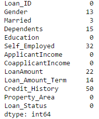 108 |
109 | *** =instructions
110 | Apply isnull().sum() with test dataset
111 |
112 |
113 |
114 | *** =hint
115 | Use train.isnull().sum() to check number of missing values in train data set
116 |
117 |
118 |
119 | *** =pre_exercise_code
120 |
121 | ```{python}
122 |
123 | # The pre-exercise code runs code to initialize the user's workspace. You can use it for several things:
124 |
125 | # Import library pandas
126 | import pandas as pd
127 |
128 | # Import training file
129 | train = pd.read_csv("https://s3-ap-southeast-1.amazonaws.com/av-datahack-datacamp/train.csv")
130 |
131 | # Import testing file
132 | test = pd.read_csv("https://s3-ap-southeast-1.amazonaws.com/av-datahack-datacamp/test.csv")
133 |
134 | ```
135 |
136 | *** =sample_code
137 |
138 | ```{python}
139 |
140 | # Check variables have missing values in test data set
141 | number_missing_values_test_data = test.isnull()._____()
142 |
143 | ```
144 |
145 | *** =solution
146 |
147 | ```{python}
148 |
149 | # Check variables have missing values in test data set
150 | number_missing_values_test_data = test.isnull().sum()
151 |
152 | ```
153 |
154 | *** =sct
155 |
156 | ```{python}
157 | # The sct section defines the Submission Correctness Tests (SCTs) used to
158 | # evaluate the student's response. All functions used here are defined in the
159 | # pythonwhat Python package. Documentation can also be found at github.com/datacamp/pythonwhat/wiki
160 |
161 | # Check variables have missing values in test data set
162 | test_object("number_missing_values_test_data", incorrect_msg='Have you count the number of missing values in each variable of test data set?')
163 |
164 |
165 | success_msg("Great work!")
166 | ```
167 |
168 |
169 | --- type:NormalExercise lang:python xp:100 skills:2, 4, 8 key:fd3cdcb726
170 | ## Imputing missing values of LoanAmount
171 |
172 | There are multiple ways to fill the missing values of continuous variables. You can replace them with mean, median or estimate values based on other features of the data set.
173 |
174 | For the sake of simplicity, we would impute the missing values of LoanAmount by mean value (Mean of available values of LoanAmount).
175 |
176 | ```{python}
177 | train['LoanAmount'].fillna(train['LoanAmount'].mean(), inplace=True)
178 | ```
179 |
180 | *** =instructions
181 | Impute missing values with a specific value 168
182 |
183 |
184 |
185 |
186 |
187 | *** =hint
188 | Use dataframe['missingcol'].fillna(225, inplace=True) to impute missing value of column 'missingcol' with 225
189 |
190 |
191 | *** =pre_exercise_code
192 |
193 | ```{python}
194 |
195 | # The pre-exercise code runs code to initialize the user's workspace. You can use it for several things:
196 |
197 | # Import library pandas
198 | import pandas as pd
199 |
200 | # Import training file
201 | train = pd.read_csv("https://s3-ap-southeast-1.amazonaws.com/av-datahack-datacamp/train.csv")
202 |
203 | # Import testing file
204 | test = pd.read_csv("https://s3-ap-southeast-1.amazonaws.com/av-datahack-datacamp/test.csv")
205 |
206 | ```
207 |
208 | *** =sample_code
209 |
210 | ```{python}
211 |
212 | # Impute missing value of LoanAmount with 168 for test data set
213 | test['LoanAmount'].fillna(______, inplace=True)
214 |
215 | ```
216 |
217 | *** =solution
218 |
219 | ```{python}
220 |
221 | # Impute missing value of LoanAmount with 168 for test data set
222 | test['LoanAmount'].fillna(168, inplace=True)
223 |
224 | ```
225 |
226 | *** =sct
227 |
228 | ```{python}
229 | # The sct section defines the Submission Correctness Tests (SCTs) used to
230 | # evaluate the student's response. All functions used here are defined in the
231 | # pythonwhat Python package. Documentation can also be found at github.com/datacamp/pythonwhat/wiki
232 |
233 | # Impute missing value of LoanAmount with 168 for test data set
234 | test_data_frame("test", columns=["LoanAmount"], incorrect_msg='Did you impute missing value with 168?')
235 | success_msg("Great work!")
236 | ```
237 |
238 |
239 | --- type:NormalExercise lang:python xp:100 skills:2, 4, 8 key:ca19896cae
240 | ## Impute missing values of SelfEmployed
241 |
242 | Similarly, to impute missing values of Categorical variables, we look at the frequency table. The simplest way is to impute with value which has highest frequency because there is a higher probability of success.
243 |
244 | For example, if you look at the distribution of SelfEmployed 500 out of 582 which is ~86% of total values falls under the category "No". Here we will replace missing values of SelfEmployed with "No".
245 |
246 | ```{python}
247 | train['Self_Employed'].fillna('No',inplace=True)
248 | ```
249 |
250 | *** =instructions
251 | - Impute missing values with more frequent category of Gender and Credit History
252 | - Use value_counts() to check more frequent category of variable
253 |
254 | *** =hint
255 | - Male is more frequent in Gender
256 | - 1 is more frequent in Credit_History
257 |
258 |
259 | *** =pre_exercise_code
260 |
261 | ```{python}
262 |
263 | # The pre-exercise code runs code to initialize the user's workspace. You can use it for several things:
264 |
265 | # Import library pandas
266 | import pandas as pd
267 |
268 | # Import training file
269 | train = pd.read_csv("https://s3-ap-southeast-1.amazonaws.com/av-datahack-datacamp/train.csv")
270 |
271 | # Import testing file
272 | test = pd.read_csv("https://s3-ap-southeast-1.amazonaws.com/av-datahack-datacamp/test.csv")
273 |
274 | ```
275 |
276 | *** =sample_code
277 |
278 | ```{python}
279 |
280 | # Impute missing value of Gender (Male is more frequent category)
281 | train['Gender'].fillna(_____,inplace=True)
282 |
283 |
284 | # Impute missing value of Credit_History ( 1 is more frequent category)
285 | train['Credit_History'].fillna(_____,inplace=True)
286 |
287 | ```
288 |
289 | *** =solution
290 |
291 | ```{python}
292 |
293 | # Impute missing value of LoanAmount with median for test data set
294 | train['Gender'].fillna('Male',inplace=True)
295 |
296 | # Impute missing value of Credit_History
297 | train['Credit_History'].fillna(1,inplace=True)
298 |
299 |
300 | ```
301 |
302 | *** =sct
303 |
304 | ```{python}
305 | # The sct section defines the Submission Correctness Tests (SCTs) used to
306 | # evaluate the student's response. All functions used here are defined in the
307 | # pythonwhat Python package. Documentation can also be found at github.com/datacamp/pythonwhat/wiki
308 |
309 | # Impute missing value of LoanAmount with median for test data set
310 | test_data_frame("train", columns=["Gender"], incorrect_msg='Did you impute missing value of Gender with Male?')
311 |
312 | # Impute missing value of Credit_History
313 | test_data_frame("train", columns=["Credit_History"], incorrect_msg='Did you impute missing value of Credit_History with 1?')
314 |
315 |
316 | success_msg("Great work!")
317 | ```
318 | --- type:NormalExercise lang:python xp:100 skills:2, 4, 8 key:2607b0ce32
319 |
320 | ## Treat / Tranform extreme values of LoanAmount and ApplicantIncome
321 |
322 | Let’s analyze LoanAmount first. Since the extreme values are practically possible, i.e. some people might apply for high-value loans due to specific needs.
323 |
324 | ```{python}
325 | train ['LoanAmount'].hist(bins=20)
326 | ```
327 |
108 |
109 | *** =instructions
110 | Apply isnull().sum() with test dataset
111 |
112 |
113 |
114 | *** =hint
115 | Use train.isnull().sum() to check number of missing values in train data set
116 |
117 |
118 |
119 | *** =pre_exercise_code
120 |
121 | ```{python}
122 |
123 | # The pre-exercise code runs code to initialize the user's workspace. You can use it for several things:
124 |
125 | # Import library pandas
126 | import pandas as pd
127 |
128 | # Import training file
129 | train = pd.read_csv("https://s3-ap-southeast-1.amazonaws.com/av-datahack-datacamp/train.csv")
130 |
131 | # Import testing file
132 | test = pd.read_csv("https://s3-ap-southeast-1.amazonaws.com/av-datahack-datacamp/test.csv")
133 |
134 | ```
135 |
136 | *** =sample_code
137 |
138 | ```{python}
139 |
140 | # Check variables have missing values in test data set
141 | number_missing_values_test_data = test.isnull()._____()
142 |
143 | ```
144 |
145 | *** =solution
146 |
147 | ```{python}
148 |
149 | # Check variables have missing values in test data set
150 | number_missing_values_test_data = test.isnull().sum()
151 |
152 | ```
153 |
154 | *** =sct
155 |
156 | ```{python}
157 | # The sct section defines the Submission Correctness Tests (SCTs) used to
158 | # evaluate the student's response. All functions used here are defined in the
159 | # pythonwhat Python package. Documentation can also be found at github.com/datacamp/pythonwhat/wiki
160 |
161 | # Check variables have missing values in test data set
162 | test_object("number_missing_values_test_data", incorrect_msg='Have you count the number of missing values in each variable of test data set?')
163 |
164 |
165 | success_msg("Great work!")
166 | ```
167 |
168 |
169 | --- type:NormalExercise lang:python xp:100 skills:2, 4, 8 key:fd3cdcb726
170 | ## Imputing missing values of LoanAmount
171 |
172 | There are multiple ways to fill the missing values of continuous variables. You can replace them with mean, median or estimate values based on other features of the data set.
173 |
174 | For the sake of simplicity, we would impute the missing values of LoanAmount by mean value (Mean of available values of LoanAmount).
175 |
176 | ```{python}
177 | train['LoanAmount'].fillna(train['LoanAmount'].mean(), inplace=True)
178 | ```
179 |
180 | *** =instructions
181 | Impute missing values with a specific value 168
182 |
183 |
184 |
185 |
186 |
187 | *** =hint
188 | Use dataframe['missingcol'].fillna(225, inplace=True) to impute missing value of column 'missingcol' with 225
189 |
190 |
191 | *** =pre_exercise_code
192 |
193 | ```{python}
194 |
195 | # The pre-exercise code runs code to initialize the user's workspace. You can use it for several things:
196 |
197 | # Import library pandas
198 | import pandas as pd
199 |
200 | # Import training file
201 | train = pd.read_csv("https://s3-ap-southeast-1.amazonaws.com/av-datahack-datacamp/train.csv")
202 |
203 | # Import testing file
204 | test = pd.read_csv("https://s3-ap-southeast-1.amazonaws.com/av-datahack-datacamp/test.csv")
205 |
206 | ```
207 |
208 | *** =sample_code
209 |
210 | ```{python}
211 |
212 | # Impute missing value of LoanAmount with 168 for test data set
213 | test['LoanAmount'].fillna(______, inplace=True)
214 |
215 | ```
216 |
217 | *** =solution
218 |
219 | ```{python}
220 |
221 | # Impute missing value of LoanAmount with 168 for test data set
222 | test['LoanAmount'].fillna(168, inplace=True)
223 |
224 | ```
225 |
226 | *** =sct
227 |
228 | ```{python}
229 | # The sct section defines the Submission Correctness Tests (SCTs) used to
230 | # evaluate the student's response. All functions used here are defined in the
231 | # pythonwhat Python package. Documentation can also be found at github.com/datacamp/pythonwhat/wiki
232 |
233 | # Impute missing value of LoanAmount with 168 for test data set
234 | test_data_frame("test", columns=["LoanAmount"], incorrect_msg='Did you impute missing value with 168?')
235 | success_msg("Great work!")
236 | ```
237 |
238 |
239 | --- type:NormalExercise lang:python xp:100 skills:2, 4, 8 key:ca19896cae
240 | ## Impute missing values of SelfEmployed
241 |
242 | Similarly, to impute missing values of Categorical variables, we look at the frequency table. The simplest way is to impute with value which has highest frequency because there is a higher probability of success.
243 |
244 | For example, if you look at the distribution of SelfEmployed 500 out of 582 which is ~86% of total values falls under the category "No". Here we will replace missing values of SelfEmployed with "No".
245 |
246 | ```{python}
247 | train['Self_Employed'].fillna('No',inplace=True)
248 | ```
249 |
250 | *** =instructions
251 | - Impute missing values with more frequent category of Gender and Credit History
252 | - Use value_counts() to check more frequent category of variable
253 |
254 | *** =hint
255 | - Male is more frequent in Gender
256 | - 1 is more frequent in Credit_History
257 |
258 |
259 | *** =pre_exercise_code
260 |
261 | ```{python}
262 |
263 | # The pre-exercise code runs code to initialize the user's workspace. You can use it for several things:
264 |
265 | # Import library pandas
266 | import pandas as pd
267 |
268 | # Import training file
269 | train = pd.read_csv("https://s3-ap-southeast-1.amazonaws.com/av-datahack-datacamp/train.csv")
270 |
271 | # Import testing file
272 | test = pd.read_csv("https://s3-ap-southeast-1.amazonaws.com/av-datahack-datacamp/test.csv")
273 |
274 | ```
275 |
276 | *** =sample_code
277 |
278 | ```{python}
279 |
280 | # Impute missing value of Gender (Male is more frequent category)
281 | train['Gender'].fillna(_____,inplace=True)
282 |
283 |
284 | # Impute missing value of Credit_History ( 1 is more frequent category)
285 | train['Credit_History'].fillna(_____,inplace=True)
286 |
287 | ```
288 |
289 | *** =solution
290 |
291 | ```{python}
292 |
293 | # Impute missing value of LoanAmount with median for test data set
294 | train['Gender'].fillna('Male',inplace=True)
295 |
296 | # Impute missing value of Credit_History
297 | train['Credit_History'].fillna(1,inplace=True)
298 |
299 |
300 | ```
301 |
302 | *** =sct
303 |
304 | ```{python}
305 | # The sct section defines the Submission Correctness Tests (SCTs) used to
306 | # evaluate the student's response. All functions used here are defined in the
307 | # pythonwhat Python package. Documentation can also be found at github.com/datacamp/pythonwhat/wiki
308 |
309 | # Impute missing value of LoanAmount with median for test data set
310 | test_data_frame("train", columns=["Gender"], incorrect_msg='Did you impute missing value of Gender with Male?')
311 |
312 | # Impute missing value of Credit_History
313 | test_data_frame("train", columns=["Credit_History"], incorrect_msg='Did you impute missing value of Credit_History with 1?')
314 |
315 |
316 | success_msg("Great work!")
317 | ```
318 | --- type:NormalExercise lang:python xp:100 skills:2, 4, 8 key:2607b0ce32
319 |
320 | ## Treat / Tranform extreme values of LoanAmount and ApplicantIncome
321 |
322 | Let’s analyze LoanAmount first. Since the extreme values are practically possible, i.e. some people might apply for high-value loans due to specific needs.
323 |
324 | ```{python}
325 | train ['LoanAmount'].hist(bins=20)
326 | ```
327 | 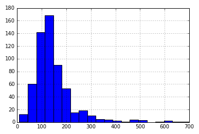 328 |
329 | So instead of treating them as outliers, let’s try a log transformation to nullify their effect:
330 |
331 | ```{python}
332 | import numpy as np
333 | train ['LoanAmount_log'] = np.log(train['LoanAmount'])
334 | train ['LoanAmount_log'].hist(bins=20)
335 | ```
336 |
328 |
329 | So instead of treating them as outliers, let’s try a log transformation to nullify their effect:
330 |
331 | ```{python}
332 | import numpy as np
333 | train ['LoanAmount_log'] = np.log(train['LoanAmount'])
334 | train ['LoanAmount_log'].hist(bins=20)
335 | ```
336 | 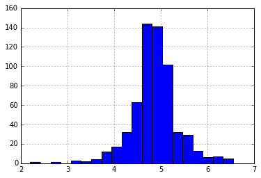 337 |
338 |
339 | Now the distribution looks much closer to normal and effect of extreme values has been significantly subsided.
340 |
341 | *** =instructions
342 | - Add both ApplicantIncome and CoapplicantIncome as TotalIncome
343 | - Take log transformation of TotalIncome to deal with extreme values
344 |
345 |
346 | *** =hint
347 | - Add both train['ApplicantIncome'] and train['CoapplicantIncome']
348 | - Take log of df['TotalIncome']
349 |
350 |
351 | *** =pre_exercise_code
352 |
353 | ```{python}
354 |
355 | # The pre-exercise code runs code to initialize the user's workspace. You can use it for several things:
356 |
357 | # Import library pandas
358 | import pandas as pd
359 | import numpy as np
360 |
361 | # Import training file
362 | train = pd.read_csv("https://s3-ap-southeast-1.amazonaws.com/av-datahack-datacamp/train.csv")
363 |
364 | # Import testing file
365 | test = pd.read_csv("https://s3-ap-southeast-1.amazonaws.com/av-datahack-datacamp/test.csv")
366 | train['TotalIncome'] = train['ApplicantIncome'] + train['CoapplicantIncome']
367 |
368 | ```
369 |
370 | *** =sample_code
371 |
372 | ```{python}
373 |
374 | # Training and Testing datasets are loaded in variable train and test dataframe respectively
375 |
376 | # Add both ApplicantIncome and CoapplicantIncome to TotalIncome
377 | train['TotalIncome'] = train['ApplicantIncome'] + train[_________]
378 |
379 | # Perform log transformation of TotalIncome to make it closer to normal
380 | train['TotalIncome_log']= np.____(train['TotalIncome'])
381 |
382 |
383 | ```
384 |
385 | *** =solution
386 |
387 | ```{python}
388 |
389 | # Training and Testing datasets are loaded in variable train and test dataframe respectively
390 |
391 | # Add both ApplicantIncome and CoapplicantIncome to TotalIncome
392 | train['TotalIncome'] = train['ApplicantIncome'] + train['CoapplicantIncome']
393 |
394 | # Perform log transformation of TotalIncome to make it closer to normal
395 | train['TotalIncome_log'] = np.log(train['TotalIncome'])
396 |
397 |
398 | ```
399 |
400 | *** =sct
401 |
402 | ```{python}
403 | # The sct section defines the Submission Correctness Tests (SCTs) used to
404 | # evaluate the student's response. All functions used here are defined in the
405 | # pythonwhat Python package. Documentation can also be found at github.com/datacamp/pythonwhat/wiki
406 |
407 | # Add both ApplicantIncome and CoapplicantIncome to TotalIncome
408 | test_data_frame("train", columns=["TotalIncome"], incorrect_msg='Have you added both ApplicantIncome and CoapplicantIncome?')
409 |
410 | # Perform log transformation of TotalIncome to make it closer to normal
411 | test_data_frame("train", columns=["TotalIncome_log"], incorrect_msg='Have you taken log of TotalIncome?')
412 |
413 | success_msg("Great work!")
414 | ```
415 |
416 | --- type:MultipleChoiceExercise lang:python xp:50 skills:2 key:9a8fd577a9
417 | ## iPython / Jupyter notebook for Data Exploration
418 |
419 | The Jupyter Notebook is a web application that allows you to create and share documents that contain live code, equations, visualizations and explanatory text. Uses include: data cleaning and transformation, numerical simulation, statistical modeling, machine learning and much more.
420 |
421 | We have shared the Jupyter notebook for your reference here
422 |
423 | ### Download the jupyter notebook from here. Have you downloaded the jupyter notebook?
424 |
425 | *** =instructions
426 | - Yes, I have downloaded the notebook
427 | - No, I am not able to
428 |
429 | *** =hint
430 | Click on the link and download the Jupyter notebook.
431 |
432 | *** =sct
433 | ```{python}
434 | # The sct section defines the Submission Correctness Tests (SCTs) used to
435 | # evaluate the student's response. All functions used here are defined in the
436 | # pythonwhat Python package
437 |
438 | msg1 = "Awesome! You can proceed to model building now!"
439 | msg2 = "Check the link provided and download the file from there."
440 |
441 | # Use test_mc() to grade multiple choice exercises.
442 | # Pass the correct option (Action, option 2 in the instructions) to correct.
443 | # Pass the feedback messages, both positive and negative, to feedback_msgs in the appropriate order.
444 | test_mc(1, [msg1, msg2])
445 |
446 | ```
447 |
--------------------------------------------------------------------------------
/chapter5.md:
--------------------------------------------------------------------------------
1 | ---
2 | title : Building a Predictive model in Python
3 | description : We build our predictive models and make submissions to the AV DataHack platform in this section.
4 |
5 | --- type:MultipleChoiceExercise lang:python xp:50 skills:2, 6 key:9a8fd577a9
6 | ## First Step of Model Building
7 |
8 | In Python, Scikit-Learn (sklearn) is the most commonly used library for building predictive / machine learning models. This article provides a good overview of scikit-learn. It has gathered a lot of interest recently for model building. There are few pre-requisite before jumping into a model building exercise:
9 |
10 | * Treat missing values
11 | * Treat outlier/ exponential observation
12 | * All inputs must be numeric array ( Requirement of scikit learn library)
13 |
14 |
15 | ####Can we build a model without treating missing values of a data set?
16 |
17 |
18 | *** =instructions
19 | - True
20 | - False
21 |
22 | *** =hint
23 | Missing value tratment is mandatory step of model building
24 |
25 |
26 | *** =sct
27 | ```{python}
28 | # The sct section defines the Submission Correctness Tests (SCTs) used to
29 | # evaluate the student's response. All functions used here are defined in the
30 | # pythonwhat Python package
31 |
32 | msg_bad1 = "Think again - If the values are missing, how will you make a predictive model?"
33 | msg_success = "Yes! We should always treat missing value"
34 |
35 | # Use test_mc() to grade multiple choice exercises.
36 | # Pass the correct option (Action, option 2 in the instructions) to correct.
37 | # Pass the feedback messages, both positive and negative, to feedback_msgs in the appropriate order.
38 | test_mc(2, [msg_bad1, msg_success])
39 | ```
40 |
41 |
42 |
43 | --- type:NormalExercise lang:python xp:100 skills:2, 6 key:2c1cf7aa90
44 | ## Label categories of Gender to number
45 |
46 | Library "Scikit Learn" only works with numeric array. Hence, we need to label all the character variables into a numeric array. For example Variable "Gender" has two labels "Male" and "Female". Hence, we will transform the labels to number as 1 for "Male" and 0 for "Female".
47 |
48 | "Scikit Learn" library has a module called "LabelEncoder" which helps to label character labels into numbers so first import module "LabelEncoder".
49 |
50 | ```{python}
51 |
52 | from sklearn.preprocessing import LabelEncoder
53 |
54 | number = LabelEncoder()
55 |
56 | train['Gender'] = number.fit_transform(train['Gender'].astype(str))
57 |
58 | ```
59 |
60 | *** =instructions
61 | Perform Label encoding for categories of variable "Married" and save it as a new variable "Married_new" in the DataFrame
62 |
63 |
64 | *** =hint
65 | Use number.fit_transform() to perform label encoding
66 |
67 |
68 | *** =pre_exercise_code
69 |
70 | ```{python}
71 |
72 | # The pre exercise code runs code to initialize the user's workspace. You can use it for several things:
73 |
74 | # Import library pandas
75 | import pandas as pd
76 | import numpy as np
77 | from sklearn.preprocessing import LabelEncoder
78 |
79 | # Import training file
80 | train = pd.read_csv("https://s3-ap-southeast-1.amazonaws.com/av-datahack-datacamp/train.csv")
81 |
82 | # Import testing file
83 | test = pd.read_csv("https://s3-ap-southeast-1.amazonaws.com/av-datahack-datacamp/test.csv")
84 |
85 | ```
86 |
87 | *** =sample_code
88 |
89 | ```{python}
90 |
91 | #import module for label encoding
92 | from sklearn.preprocessing import LabelEncoder
93 |
94 | #train and test dataset is already loaded in the enviornment
95 | # Perform label encoding for variable 'Married'
96 | number = LabelEncoder()
97 | train['Married_new'] = number.________(train['Married'].astype(str))
98 |
99 |
100 | ```
101 |
102 | *** =solution
103 |
104 | ```{python}
105 |
106 | #import module for label encoding
107 | from sklearn.preprocessing import LabelEncoder
108 |
109 | #train and test dataset is already loaded in the enviornment
110 | # Perform label encoding for variable 'Married'
111 | number = LabelEncoder()
112 | train['Married_new'] = number.fit_transform(train['Married'].astype(str))
113 | ```
114 |
115 | *** =sct
116 |
117 | ```{python}
118 | # The sct section defines the Submission Correctness Tests (SCTs) used to
119 | # evaluate the student's response. All functions used here are defined in the
120 | # pythonwhat Python package. Documentation can also be found at github.com/datacamp/pythonwhat/wiki
121 |
122 | # Perform label encoding for Married
123 | test_data_frame("train", columns=["Married"], incorrect_msg='Have you used write methds to perform label encoding for variable Married?')
124 |
125 | success_msg("Great work!")
126 | ```
127 |
128 |
129 | --- type:MultipleChoiceExercise lang:python xp:50 skills:2, 6 key:ee5ed17633
130 | ## Selecting the right algorithm
131 |
132 | The basic principle behind selecting the right algorithm is to look at the dependent variable (or target variable). In this challenge "Loan Prediction", we need to classify a customer's eligibility for Loan as "Y" or "N" based on the available information about the customer. Here the dependent variable is categorical and our task is to classify the customer in two groups; eligible for the loan amount and not eligible for the loan amount.
133 |
134 | This is a classification challenge so we will import module of classification algorithms of sklearn library. Below are some commonly used classification algorithms:
135 | * Logistic Regression
136 | * Decision Tree
137 | * Random Forest
138 |
139 |
140 | ####Whether an e-mail is spam or not? Is this problem a classification challenge or regression?
141 |
142 |
143 | *** =instructions
144 | - Classification
145 | - Regression
146 |
147 | *** =hint
148 | - Regression: When we model for continuous variables
149 | - Classification: When we model to classify in different categories
150 |
151 |
152 |
153 |
154 | *** =sct
155 | ```{python}
156 | # The sct section defines the Submission Correctness Tests (SCTs) used to
157 | # evaluate the student's response. All functions used here are defined in the
158 | # pythonwhat Python package
159 |
160 | msg_bad1 = "Try again. Regression challenges require you to predict a quantity, while classification challenge requires you to classify an object in groups."
161 | msg_success = "Correct - this is a classification challenge"
162 |
163 | # Use test_mc() to grade multiple choice exercises.
164 | # Pass the correct option (Action, option 2 in the instructions) to correct.
165 | # Pass the feedback messages, both positive and negative, to feedback_msgs in the appropriate order.
166 | test_mc(1, [msg_success, msg_bad1])
167 | ```
168 |
169 | --- type:MultipleChoiceExercise lang:python xp:50 skills:2, 6 key:bd9b384210
170 | ## Have you performed data preprocessing step?
171 |
172 | As discussed before, you should perform some data pre processing steps for both train and test dataset before jumping into model building exercise. Here are a few things you need to perform at the minimum:
173 | * Missing value imputation
174 | * Outlier treatment
175 | * Label encoding for character variables
176 | * Algorithm selection
177 |
178 |
179 | ####Which of the following steps have you performed till now with both train and test data set?
180 |
181 |
182 | *** =instructions
183 | - Impute missing values of all variables
184 | - Treat outlier and influential observations
185 | - Label encoding for character variables
186 | - All of the above
187 |
188 | *** =hint
189 | All steps are necessary and would impact your model performance
190 |
191 |
192 |
193 |
194 | *** =sct
195 | ```{python}
196 | # The sct section defines the Submission Correctness Tests (SCTs) used to
197 | # evaluate the student's response. All functions used here are defined in the
198 | # pythonwhat Python package
199 |
200 | msg_bad1 = "You should perform all pre processing steps before model building"
201 | msg_success = "Great! Go ahead with modeling exercise"
202 |
203 | # Use test_mc() to grade multiple choice exercises.
204 | # Pass the correct option (Action, option 2 in the instructions) to correct.
205 | # Pass the feedback messages, both positive and negative, to feedback_msgs in the appropriate order.
206 | test_mc(4, [msg_bad1, msg_bad1, msg_bad1, msg_success ])
207 | ```
208 |
209 | --- type:NormalExercise lang:python xp:100 skills:2, 6 key:f4c3fbee79
210 |
211 | ## Logistic Regression Introduction
212 |
213 | Logistic Regression is a classification algorithm. It is used to predict a binary outcome (1 / 0, Yes / No, True / False) given a set of independent variables. To represent binary / categorical outcome, we use dummy variables. You can also think of logistic regression as a special case of linear regression when the outcome variable is categorical, where we are using log of odds as the dependent variable.
214 |
215 | In simple words, it predicts the probability of occurrence of an event by fitting data to a logit function, read more about Logistic Regression .
216 |
217 | LogisticRegression() function is part of linear_model module of sklearn and is used to create logistic regression
218 |
219 | Reference: Mathematical working and implementation from scratch for Logistic regression.
220 |
221 | *** =instructions
222 | - Import Linear model of sklearn
223 | - Create object of sklearn.linear_model.LogisticRegression
224 |
225 |
226 | *** =hint
227 | You can import a module of a library as import library.module
228 |
229 | *** =pre_exercise_code
230 |
231 | ```{python}
232 | import sklearn.linear_model
233 | ```
234 |
235 | *** =sample_code
236 |
237 | ```{python}
238 |
239 | # Import linear model of sklearn
240 | import ______.linear_model
241 |
242 | # Create object of Logistic Regression
243 | model=sklearn.______.LogisticRegression()
244 |
245 | ```
246 |
247 | *** =solution
248 |
249 | ```{python}
250 | # Import linear model of sklearn
251 | import sklearn.linear_model
252 |
253 | # Create object of Logistic Regression
254 | model=sklearn.linear_model.LogisticRegression()
255 |
256 | ```
257 |
258 | *** =sct
259 |
260 | ```{python}
261 | # The sct section defines the Submission Correctness Tests (SCTs) used to
262 | # evaluate the student's response. All functions used here are defined in the
263 | # pythonwhat Python package. Documentation can also be found at github.com/datacamp/pythonwhat/wiki
264 |
265 | # Test for library import
266 | test_import("sklearn.linear_model", same_as = False)
267 |
268 | # Test for logistic regression
269 | test_function("sklearn.linear_model.LogisticRegression", incorrect_msg='Have you created Logistic Regression object from linear model module of sklearn?')
270 |
271 | success_msg("Great work!")
272 | ```
273 |
274 | --- type:NormalExercise lang:python xp:100 skills:2 key:6eb60851bc
275 |
276 | ## Build your first logistic regression model
277 |
278 | Let’s build our first Logistic Regression model. One way would be to take all the variables into the model, but this might result in overfitting (don’t worry if you’re unaware of this terminology yet). In simple words, taking all variables might result in the model understanding complex relations specific to the data and will not generalize well.
279 |
280 | We can easily make some intuitive hypothesis to set the ball rolling. The chances of getting a loan will be higher for:
281 |
282 | * Applicants having a credit history
283 | * Applicants with higher applicant and co-applicant income
284 | * Applicants with higher education level
285 | * Properties in urban areas with high growth perspectives
286 |
287 | Ok, time for you to build your first logistics regression model! The pre processed train_modified and test_modifed data are available in your workspace.
288 |
289 | *** =instructions
290 | - Store input variable in a list "predictors"
291 | - Create an object of logistic regression
292 |
293 |
294 |
295 | *** =hint
296 | Use list ['Credit_History','Education','Gender'] as predictor variable
297 |
298 | *** =pre_exercise_code
299 |
300 | ```{python}
301 | import pandas as pd
302 | import numpy as np
303 | from sklearn.preprocessing import LabelEncoder
304 |
305 | train = pd.read_csv("https://s3-ap-southeast-1.amazonaws.com/av-datahack-datacamp/train.csv")
306 | test = pd.read_csv("https://s3-ap-southeast-1.amazonaws.com/av-datahack-datacamp/test.csv")
307 |
308 | #Combining both train and test dataset
309 |
310 | train['Type']='Train' #Create a flag for Train and Test Data set
311 | test['Type']='Test'
312 | fullData = pd.concat([train,test],axis=0)
313 |
314 | #Identify categorical and continuous variables
315 |
316 | ID_col = ['Loan_ID']
317 | target_col = ["Loan_Status"]
318 | cat_cols = ['Credit_History','Dependents','Gender','Married','Education','Property_Area','Self_Employed']
319 |
320 | other_col=['Type'] #Test and Train Data set identifier
321 | num_cols= list(set(list(fullData.columns))-set(cat_cols)-set(ID_col)-set(target_col)-set(other_col))
322 |
323 | #Imputing Missing values with mean for continuous variable
324 | fullData[num_cols] = fullData[num_cols].fillna(fullData[num_cols].mean(),inplace=True)
325 |
326 |
327 | #Imputing Missing values with mode for categorical variables
328 | cat_imput=pd.Series(fullData[cat_cols].mode().values[0])
329 | cat_imput.index=cat_cols
330 | fullData[cat_cols] = fullData[cat_cols].fillna(cat_imput,inplace=True)
331 |
332 | #Create a new column as Total Income
333 | fullData['TotalIncome']=fullData['ApplicantIncome']+fullData['CoapplicantIncome']
334 |
335 | #Take a log of TotalIncome + 1, adding 1 to deal with zeros of TotalIncome it it exists
336 | fullData['Log_TotalIncome']=np.log(fullData['TotalIncome'])
337 |
338 | #create label encoders for categorical features
339 | for var in cat_cols:
340 | number = LabelEncoder()
341 | fullData[var] = number.fit_transform(fullData[var].astype('str'))
342 |
343 | train_modified=fullData[fullData['Type']=='Train']
344 | test_modified=fullData[fullData['Type']=='Test']
345 | train_modified["Loan_Status"] = number.fit_transform(train_modified["Loan_Status"].astype('str'))
346 | ```
347 |
348 | *** =sample_code
349 |
350 | ```{python}
351 |
352 | #train_modified and test_modified already loaded in the workspace
353 | #Import module for Logistic regression
354 | import sklearn.linear_model
355 |
356 | # Select three predictors Credit_History, Education and Gender
357 | predictors =[____,_____,_____]
358 |
359 | # Converting predictors and outcome to numpy array
360 | x_train = train_modified[predictors].values
361 | y_train = train_modified['Loan_Status'].values
362 |
363 | # Model Building
364 | model = sklearn.________.LogisticRegression()
365 | model.fit(x_train, y_train)
366 |
367 | ```
368 |
369 | *** =solution
370 |
371 | ```{python}
372 | # Import module for Logistic regression
373 | import sklearn.linear_model
374 |
375 | # Select three predictors Credit_History, Education and Gender
376 | predictors =['Credit_History','Education','Gender']
377 |
378 | # Converting predictors and outcome to numpy array
379 | x_train = train_modified[predictors].values
380 | y_train = train_modified['Loan_Status'].values
381 |
382 | # Model Building
383 | model = sklearn.linear_model.LogisticRegression()
384 | model.fit(x_train, y_train)
385 |
386 | ```
387 |
388 | *** =sct
389 |
390 | ```{python}
391 | # The sct section defines the Submission Correctness Tests (SCTs) used to
392 | # evaluate the student's response. All functions used here are defined in the
393 | # pythonwhat Python package. Documentation can also be found at github.com/datacamp/pythonwhat/wiki
394 |
395 | # Test for predictor selection
396 | test_object("predictors", incorrect_msg='Have you created the list of given predictors variables?')
397 |
398 | # Test for model
399 | test_function("sklearn.linear_model.LogisticRegression", incorrect_msg='Have you created Logistic Regression object from linear_model module of sklearn?')
400 |
401 | success_msg("Great work!")
402 | ```
403 |
404 |
405 |
406 | --- type:NormalExercise lang:python xp:100 skills:2, 6 key:207a5629cc
407 |
408 | ## Prediction and submission to DataHack
409 |
410 | To upload a submission to DataHack, you need to predict the loan approval rate for the observations in the test set. This can be done using ".predict()" method with logistic regression object (model). To extract the test features we will need to create a numpy array of input features of test data set in the same way as we did when training the model for training data.
411 |
412 | Next, you need to make sure your output is in line with the submission requirements of DataHack: a csv file with exactly 367 entries and two columns: Loan_ID and Loan_Status. Then create a csv file using to_csv() method from Pandas.
413 |
414 |
415 | *** =instructions
416 | - Store input variable in list "predictors"
417 | - Use .predict() method for prediction
418 |
419 |
420 | *** =hint
421 | Use model.predict(x_test) for prediction of test dataset
422 |
423 | *** =pre_exercise_code
424 |
425 | ```{python}
426 | import pandas as pd
427 | import numpy as np
428 | from sklearn.preprocessing import LabelEncoder
429 |
430 | train = pd.read_csv("https://s3-ap-southeast-1.amazonaws.com/av-datahack-datacamp/train.csv")
431 | test = pd.read_csv("https://s3-ap-southeast-1.amazonaws.com/av-datahack-datacamp/test.csv")
432 |
433 | #Combining both train and test dataset
434 |
435 | train['Type']='Train' #Create a flag for Train and Test Data set
436 | test['Type']='Test'
437 | fullData = pd.concat([train,test],axis=0)
438 |
439 | #Identify categorical and continuous variables
440 |
441 | ID_col = ['Loan_ID']
442 | target_col = ["Loan_Status"]
443 | cat_cols = ['Credit_History','Dependents','Gender','Married','Education','Property_Area','Self_Employed']
444 |
445 | other_col=['Type'] #Test and Train Data set identifier
446 | num_cols= list(set(list(fullData.columns))-set(cat_cols)-set(ID_col)-set(target_col)-set(other_col))
447 |
448 | #Imputing Missing values with mean for continuous variable
449 | fullData[num_cols] = fullData[num_cols].fillna(fullData[num_cols].mean(),inplace=True)
450 |
451 |
452 | #Imputing Missing values with mode for categorical variables
453 | cat_imput=pd.Series(fullData[cat_cols].mode().values[0])
454 | cat_imput.index=cat_cols
455 | fullData[cat_cols] = fullData[cat_cols].fillna(cat_imput,inplace=True)
456 |
457 | #Create a new column as Total Income
458 |
459 | fullData['TotalIncome']=fullData['ApplicantIncome']+fullData['CoapplicantIncome']
460 |
461 | #Take a log of TotalIncome + 1, adding 1 to deal with zeros of TotalIncome it it exists
462 | fullData['Log_TotalIncome']=np.log(fullData['TotalIncome'])
463 |
464 | #create label encoders for categorical features
465 | for var in cat_cols:
466 | number = LabelEncoder()
467 | fullData[var] = number.fit_transform(fullData[var].astype('str'))
468 |
469 | train_modified=fullData[fullData['Type']=='Train']
470 | test_modified=fullData[fullData['Type']=='Test']
471 | train_modified["Loan_Status"] = number.fit_transform(train_modified["Loan_Status"].astype('str'))
472 |
473 | # Import module for Logistic regression
474 | from sklearn.linear_model import LogisticRegression
475 |
476 | # Select three predictors Credit_History, Education and Gender
477 | predictors =['Credit_History','Education','Gender']
478 |
479 | # Converting predictors and outcome to numpy array
480 | x_train = train_modified[predictors].values
481 | y_train = train_modified['Loan_Status'].values
482 |
483 | # Model Building
484 | model = LogisticRegression()
485 | model.fit(x_train, y_train)
486 | ```
487 |
488 | *** =sample_code
489 |
490 | ```{python}
491 |
492 | #test_modified already loaded in the workspace
493 |
494 | # Select three predictors Credit_History, Education and Gender
495 | predictors =[____,_____,_____]
496 |
497 | # Converting predictors and outcome to numpy array
498 | x_test = test_modified[predictors].values
499 |
500 | #Predict Output
501 | predicted= model._____(x_test)
502 |
503 | #Reverse encoding for predicted outcome
504 | predicted = number.inverse_transform(predicted)
505 |
506 | #Store it to test dataset
507 | test_modified['Loan_Status']=predicted
508 |
509 | #Output file to make submission
510 | test_modified.to_csv("Submission1.csv",columns=['Loan_ID','Loan_Status'])
511 |
512 | ```
513 |
514 | *** =solution
515 |
516 | ```{python}
517 | #test_modified already loaded in the workspace
518 |
519 | # Select three predictors Credit_History, Education and Gender
520 | predictors =['Credit_History','Education','Gender']
521 |
522 | # Converting predictors and outcome to numpy array
523 | x_test = test_modified[predictors].values
524 |
525 | #Predict Output
526 | predicted= model.predict(x_test)
527 |
528 | #Reverse encoding for predicted outcome
529 | predicted = number.inverse_transform(predicted)
530 |
531 | #Store it to test dataset
532 | test_modified['Loan_Status']=predicted
533 |
534 | #Output file to make submission
535 | test_modified.to_csv("Submission1.csv",columns=['Loan_ID','Loan_Status'])
536 |
537 | ```
538 |
539 | *** =sct
540 |
541 | ```{python}
542 | # The sct section defines the Submission Correctness Tests (SCTs) used to
543 | # evaluate the student's response. All functions used here are defined in the
544 | # pythonwhat Python package. Documentation can also be found at github.com/datacamp/pythonwhat/wiki
545 |
546 | # Test for predictor selection
547 | test_object("predictors", incorrect_msg='Have you create the list of given predictors variables?')
548 |
549 | # Test for model
550 | test_object("predicted", incorrect_msg='Have you used .predict() method?')
551 |
552 | success_msg("Great work!")
553 | ```
554 |
555 | --- type:NormalExercise lang:python xp:100 skills:2, 6 key:0f04d6b3e1
556 |
557 | ## Decision Tree Introduction
558 |
559 | Decision trees are mostly used in classification problems. It works for both categorical and continuous input and output variables. In this technique, we split the population or sample into two or more homogeneous sets (or sub-populations) based on most significant splitter / differentiator in input variables, read more about Decision Tree .
560 |
561 |
562 | *** =instructions
563 | - Import tree module of sklearn
564 | - Create a object of DecisionTreeClassifier
565 |
566 |
567 | *** =hint
568 | Use DecisiontreeClassifier() with sklearn.tree to create object of decision tree
569 |
570 | *** =pre_exercise_code
571 |
572 | ```{python}
573 | from sklearn.tree import DecisionTreeClassifier
574 |
575 | ```
576 |
577 | *** =sample_code
578 |
579 | ```{python}
580 |
581 | # Import tree module of sklearn
582 | import sklearn._____
583 |
584 | # Create object of DecisionTreeClassifier
585 | model = sklearn.tree.__________()
586 |
587 | ```
588 |
589 | *** =solution
590 |
591 | ```{python}
592 | # Import tree module of sklearn
593 | import sklearn.tree
594 |
595 | # Create object of DecisionTreeClassifier
596 | model = sklearn.tree.DecisionTreeClassifier()
597 |
598 | ```
599 |
600 | *** =sct
601 |
602 | ```{python}
603 | # The sct section defines the Submission Correctness Tests (SCTs) used to
604 | # evaluate the student's response. All functions used here are defined in the
605 | # pythonwhat Python package. Documentation can also be found at github.com/datacamp/pythonwhat/wiki
606 |
607 | # Test for library import
608 | test_import("sklearn.tree", same_as = False)
609 |
610 | # Test for logistic regression
611 | test_function("sklearn.tree.DecisionTreeClassifier", incorrect_msg='Have you created DecisionTree object from tree module of sklearn?')
612 |
613 | success_msg("Great work!")
614 | ```
615 |
616 |
617 |
618 | --- type:NormalExercise lang:python xp:100 skills:2, 4, 6 key:dcf5c3e2c2
619 |
620 | ## Train model and do prediction using Decision Tree
621 |
622 | Let’s make first Decision Tree model. Similar to Logistic regression, we first select the input features, train our model and finally perform prediction on test data set.
623 |
624 | Ok! time for you to build your first Decision Tree model! The pre processed train_modified and test_modifed data are available in your workspace.
625 |
626 |
627 | *** =instructions
628 | - Store input variable in list "predictors"
629 | - Create a object of DecisionTreeClassifier
630 | - Do prediction for test data set
631 | - Export test prediction to csv file
632 |
633 |
634 | *** =hint
635 | - Use predictors =['Credit_History','Education','Gender'] as predictor variable
636 | - Use DecisionTreeClassifier with sklearn.tree to create decision tree object
637 | - Use to_csv() with dataframe to export csv file
638 |
639 |
640 | *** =pre_exercise_code
641 |
642 | ```{python}
643 | import pandas as pd
644 | import numpy as np
645 | from sklearn.preprocessing import LabelEncoder
646 | import sklearn.tree
647 |
648 | train = pd.read_csv("https://s3-ap-southeast-1.amazonaws.com/av-datahack-datacamp/train.csv")
649 | test = pd.read_csv("https://s3-ap-southeast-1.amazonaws.com/av-datahack-datacamp/test.csv")
650 |
651 | #Combining both train and test dataset
652 |
653 | train['Type']='Train' #Create a flag for Train and Test Data set
654 | test['Type']='Test'
655 | fullData = pd.concat([train,test],axis=0)
656 |
657 | #Identify categorical and continuous variables
658 |
659 | ID_col = ['Loan_ID']
660 | target_col = ["Loan_Status"]
661 | cat_cols = ['Credit_History','Dependents','Gender','Married','Education','Property_Area','Self_Employed']
662 |
663 | other_col=['Type'] #Test and Train Data set identifier
664 | num_cols= list(set(list(fullData.columns))-set(cat_cols)-set(ID_col)-set(target_col)-set(other_col))
665 |
666 | #Imputing Missing values with mean for continuous variable
667 | fullData[num_cols] = fullData[num_cols].fillna(fullData[num_cols].mean(),inplace=True)
668 |
669 |
670 | #Imputing Missing values with mode for categorical variables
671 | cat_imput=pd.Series(fullData[cat_cols].mode().values[0])
672 | cat_imput.index=cat_cols
673 | fullData[cat_cols] = fullData[cat_cols].fillna(cat_imput,inplace=True)
674 |
675 | #Create a new column as Total Income
676 | fullData['TotalIncome']=fullData['ApplicantIncome']+fullData['CoapplicantIncome']
677 |
678 | #Take a log of TotalIncome + 1, adding 1 to deal with zeros of TotalIncome it it exists
679 | fullData['Log_TotalIncome']=np.log(fullData['TotalIncome'])
680 |
681 | #create label encoders for categorical features
682 | for var in cat_cols:
683 | number = LabelEncoder()
684 | fullData[var] = number.fit_transform(fullData[var].astype('str'))
685 |
686 | train_modified=fullData[fullData['Type']=='Train']
687 | test_modified=fullData[fullData['Type']=='Test']
688 | train_modified["Loan_Status"] = number.fit_transform(train_modified["Loan_Status"].astype('str'))
689 | ```
690 |
691 | *** =sample_code
692 |
693 | ```{python}
694 |
695 | #train_modified and test_modified already loaded in the workspace
696 | #Import module for Decision tree
697 | import sklearn.tree
698 |
699 | # Select three predictors Credit_History, Education and Gender
700 | predictors =[____,_____,_____]
701 |
702 | # Converting predictors and outcome to numpy array
703 | x_train = train_modified[predictors].values
704 | y_train = train_modified['Loan_Status'].values
705 |
706 | # Model Building
707 | model = sklearn._____.DecisionTreeClassifier()
708 | model.fit(x_train, y_train)
709 |
710 | # Converting predictors and outcome to numpy array
711 | x_test = test_modified[predictors].values
712 |
713 | #Predict Output
714 | predicted= model._____(x_test)
715 |
716 | #Reverse encoding for predicted outcome
717 | predicted = number.inverse_transform(predicted)
718 |
719 | #Store it to test dataset
720 | test_modified['Loan_Status']=predicted
721 |
722 | #Output file to make submission
723 | test_modified.______("Submission1.csv",columns=['Loan_ID','Loan_Status'])
724 |
725 |
726 | ```
727 |
728 | *** =solution
729 |
730 | ```{python}
731 | #train_modified and test_modified already loaded in the workspace
732 | #Import module for Decision tree
733 | import sklearn.tree
734 |
735 | # Select three predictors Credit_History, Education and Gender
736 | predictors =['Credit_History','Education','Gender']
737 |
738 | # Converting predictors and outcome to numpy array
739 | x_train = train_modified[predictors].values
740 | y_train = train_modified['Loan_Status'].values
741 |
742 | # Model Building
743 | model = sklearn.tree.DecisionTreeClassifier()
744 | model.fit(x_train, y_train)
745 |
746 | # Converting predictors and outcome to numpy array
747 | x_test = test_modified[predictors].values
748 |
749 | #Predict Output
750 | predicted= model.predict(x_test)
751 |
752 | #Reverse encoding for predicted outcome
753 | predicted = number.inverse_transform(predicted)
754 |
755 | #Store it to test dataset
756 | test_modified['Loan_Status']=predicted
757 |
758 | #Output file to make submission
759 | test_modified.to_csv("Submission1.csv",columns=['Loan_ID','Loan_Status'])
760 |
761 |
762 | ```
763 |
764 | *** =sct
765 |
766 | ```{python}
767 | # The sct section defines the Submission Correctness Tests (SCTs) used to
768 | # evaluate the student's response. All functions used here are defined in the
769 | # pythonwhat Python package. Documentation can also be found at github.com/datacamp/pythonwhat/wiki
770 |
771 | # Test for predictor selection
772 | test_object("predictors", incorrect_msg='Have you create the list of given predictors variables?')
773 |
774 | # Test for model
775 | test_function("sklearn.tree.DecisionTreeClassifier", incorrect_msg='Have you created DecisionTree object from tree module of sklearn?')
776 |
777 | # Test for predicted
778 | test_object("predicted", incorrect_msg='Have you used .predict() method?')
779 |
780 |
781 | # Test for csv import
782 | test_function("test_modified.to_csv", incorrect_msg='Have you used the right function to export a csv file?')
783 |
784 | success_msg("Great work!")
785 | ```
786 |
787 |
788 |
789 |
790 |
791 | --- type:NormalExercise lang:python xp:100 skills:2, 6 key:ff4ced6565
792 |
793 | ## Random Forest Introduction
794 |
795 | Random Forest is a versatile machine learning method capable of performing both regression and classification tasks. It also undertakes dimensional reduction methods, treats missing values, outlier values and other essential steps of data exploration, and does a fairly good job. It is a type of ensemble learning method, where a group of weak models combine to form a powerful model, read more about Random Forest .
796 |
797 |
798 | *** =instructions
799 | - Import library sklearn.ensemble
800 | - Create a object of RandomForestClassifier
801 |
802 |
803 | *** =hint
804 | Use RandomForestClassifier() with sklearn.ensemble to create object of Random Forest
805 |
806 |
807 | *** =pre_exercise_code
808 |
809 | ```{python}
810 | import sklearn.ensemble
811 | ```
812 |
813 | *** =sample_code
814 |
815 | ```{python}
816 |
817 | # Import ensemble module from sklearn
818 | import sklearn.______
819 |
820 | # Create object of RandomForestClassifier
821 | model=sklearn.ensemble.__________
822 |
823 | ```
824 |
825 | *** =solution
826 |
827 | ```{python}
828 | # Import ensemble module from sklearn
829 | import sklearn.ensemble
830 |
831 | # Create object of RandomForestClassifier
832 | model=sklearn.ensemble.RandomForestClassifier()
833 |
834 | ```
835 |
836 | *** =sct
837 |
838 | ```{python}
839 | # The sct section defines the Submission Correctness Tests (SCTs) used to
840 | # evaluate the student's response. All functions used here are defined in the
841 | # pythonwhat Python package. Documentation can also be found at github.com/datacamp/pythonwhat/wiki
842 |
843 | # Test for library import
844 | test_import("sklearn.ensemble", same_as = False)
845 |
846 | # Test for logistic regression
847 | test_function("sklearn.ensemble.RandomForestClassifier", incorrect_msg='Have you created RandomForest object from ensemble module of sklearn?')
848 |
849 | success_msg("Great work!")
850 | ```
851 |
852 |
853 | --- type:NormalExercise lang:python xp:100 skills:2, 6 key:f0d1f62bb1
854 |
855 | ## Train model and do prediction using Random Forest
856 |
857 | Let’s make first Random Forest model. Similar to Logistic regression and Decision Tree, here we also first select the input features, train model and finally perform prediction on test data set.
858 |
859 | Ok, time for you to build your first Random Forest model! The pre processed train_modified and test_modifed data are available in your workspace.
860 |
861 |
862 | *** =instructions
863 | - Create a object of RandomForestClassifier
864 | - Do prediction for test data set
865 | - Export test prediction to csv file
866 |
867 |
868 | *** =hint
869 | - Use RandomForestClassifier() with sklearn.ensemble to create a random forest object
870 | - Use to_csv() with dataframe to export csv file
871 |
872 |
873 | *** =pre_exercise_code
874 |
875 | ```{python}
876 | import pandas as pd
877 | import numpy as np
878 | from sklearn.preprocessing import LabelEncoder
879 | import sklearn.ensemble
880 |
881 | train = pd.read_csv("https://s3-ap-southeast-1.amazonaws.com/av-datahack-datacamp/train.csv")
882 | test = pd.read_csv("https://s3-ap-southeast-1.amazonaws.com/av-datahack-datacamp/test.csv")
883 |
884 | #Combining both train and test dataset
885 |
886 | train['Type']='Train' #Create a flag for Train and Test Data set
887 | test['Type']='Test'
888 | fullData = pd.concat([train,test],axis=0)
889 |
890 | #Identify categorical and continuous variables
891 |
892 | ID_col = ['Loan_ID']
893 | target_col = ["Loan_Status"]
894 | cat_cols = ['Credit_History','Dependents','Gender','Married','Education','Property_Area','Self_Employed']
895 |
896 | other_col=['Type'] #Test and Train Data set identifier
897 | num_cols= list(set(list(fullData.columns))-set(cat_cols)-set(ID_col)-set(target_col)-set(other_col))
898 |
899 | #Imputing Missing values with mean for continuous variable
900 | fullData[num_cols] = fullData[num_cols].fillna(fullData[num_cols].mean(),inplace=True)
901 |
902 |
903 | #Imputing Missing values with mode for categorical variables
904 | cat_imput=pd.Series(fullData[cat_cols].mode().values[0])
905 | cat_imput.index=cat_cols
906 | fullData[cat_cols] = fullData[cat_cols].fillna(cat_imput,inplace=True)
907 |
908 | #Create a new column as Total Income
909 | fullData['TotalIncome']=fullData['ApplicantIncome']+fullData['CoapplicantIncome']
910 |
911 | #Take a log of TotalIncome + 1, adding 1 to deal with zeros of TotalIncome it it exists
912 | fullData['Log_TotalIncome']=np.log(fullData['TotalIncome'])
913 |
914 | #create label encoders for categorical features
915 | for var in cat_cols:
916 | number = LabelEncoder()
917 | fullData[var] = number.fit_transform(fullData[var].astype('str'))
918 |
919 | train_modified=fullData[fullData['Type']=='Train']
920 | test_modified=fullData[fullData['Type']=='Test']
921 | train_modified["Loan_Status"] = number.fit_transform(train_modified["Loan_Status"].astype('str'))
922 | ```
923 |
924 | *** =sample_code
925 |
926 | ```{python}
927 |
928 | #train_modified and test_modified already loaded in the workspace
929 | #Import module for Random Forest
930 | import sklearn.ensemble
931 |
932 | # Select three predictors Credit_History, Education and Gender
933 | predictors =['Credit_History','Education','Gender']
934 |
935 | # Converting predictors and outcome to numpy array
936 | x_train = train_modified[predictors].values
937 | y_train = train_modified['Loan_Status'].values
938 |
939 | # Model Building
940 | model = sklearn.ensemble._______
941 | model.fit(x_train, y_train)
942 |
943 | # Converting predictors and outcome to numpy array
944 | x_test = test_modified[predictors].values
945 |
946 | #Predict Output
947 | predicted= model.______(x_test)
948 |
949 | #Reverse encoding for predicted outcome
950 | predicted = number.inverse_transform(predicted)
951 |
952 | #Store it to test dataset
953 | test_modified['Loan_Status']=predicted
954 |
955 | #Output file to make submission
956 | test_modified._____("Submission1.csv",columns=['Loan_ID','Loan_Status'])
957 |
958 |
959 | ```
960 |
961 | *** =solution
962 |
963 | ```{python}
964 | #train_modified and test_modified already loaded in the workspace
965 | #Import module for Random Forest
966 | import sklearn.ensemble
967 |
968 | # Select three predictors Credit_History, Education and Gender
969 | predictors =['Credit_History','Education','Gender']
970 |
971 | # Converting predictors and outcome to numpy array
972 | x_train = train_modified[predictors].values
973 | y_train = train_modified['Loan_Status'].values
974 |
975 | # Model Building
976 | model = sklearn.ensemble.RandomForestClassifier()
977 | model.fit(x_train, y_train)
978 |
979 | # Converting predictors and outcome to numpy array
980 | x_test = test_modified[predictors].values
981 |
982 | #Predict Output
983 | predicted= model.predict(x_test)
984 |
985 | #Reverse encoding for predicted outcome
986 | predicted = number.inverse_transform(predicted)
987 |
988 | #Store it to test dataset
989 | test_modified['Loan_Status']=predicted
990 |
991 | #Output file to make submission
992 | test_modified.to_csv("Submission1.csv",columns=['Loan_ID','Loan_Status'])
993 |
994 |
995 | ```
996 |
997 | *** =sct
998 |
999 | ```{python}
1000 | # The sct section defines the Submission Correctness Tests (SCTs) used to
1001 | # evaluate the student's response. All functions used here are defined in the
1002 | # pythonwhat Python package. Documentation can also be found at github.com/datacamp/pythonwhat/wiki
1003 |
1004 | # Test for model
1005 | test_function("sklearn.ensemble.RandomForestClassifier", incorrect_msg='Have you created RandomForest object from ensemble module of sklearn?')
1006 |
1007 | # Test for predicted
1008 | test_object("predicted", incorrect_msg='Have you used .predict() method?')
1009 |
1010 |
1011 | # Test for csv import
1012 | test_function("test_modified.to_csv", incorrect_msg='Have you used the right function to export a csv file?')
1013 |
1014 | success_msg("Great work!")
1015 |
1016 | ```
1017 |
1018 |
1019 | --- type:MultipleChoiceExercise lang:python xp:50 skills:2, 6 key:4621632d2a
1020 | ## Selecting important variables for model building
1021 |
1022 | One of the benefits of Random forest is the power of handle large data set with higher dimensionality. It can handle thousands of input variables and identify most significant variables so it is considered as one of the dimensionality reduction methods. Further, the model outputs the importance of the variables, which can be a very handy feature.
1023 |
1024 | ```{python}
1025 |
1026 | featimp = pd.Series(model.feature_importances_, index=predictors).sort_values(ascending=False)
1027 |
1028 | print (featimp)
1029 |
1030 | ```
1031 | I have selected all the features available in the train data set and model it using random forest:
1032 |
1033 | ```{python}
1034 | predictors=['ApplicantIncome', 'CoapplicantIncome', 'Credit_History','Dependents', 'Education', 'Gender', 'LoanAmount',
1035 | 'Loan_Amount_Term', 'Married', 'Property_Area', 'Self_Employed', 'TotalIncome','Log_TotalIncome']
1036 |
1037 |
1038 | ```
1039 |
1040 | Run feature importance command and identify Which variable has the highest impact on the model??
1041 |
1042 |
1043 | *** =instructions
1044 | - LoanAmount
1045 | - Dependents
1046 | - Gender
1047 | - Education
1048 |
1049 | *** =hint
1050 | Run feature importance command
1051 |
1052 | *** =pre_exercise_code
1053 | ```{python}
1054 | import pandas as pd
1055 | import numpy as np
1056 | from sklearn.preprocessing import LabelEncoder
1057 |
1058 | train = pd.read_csv("https://s3-ap-southeast-1.amazonaws.com/av-datahack-datacamp/train.csv")
1059 | test = pd.read_csv("https://s3-ap-southeast-1.amazonaws.com/av-datahack-datacamp/test.csv")
1060 |
1061 | #Combining both train and test dataset
1062 |
1063 | train['Type']='Train' #Create a flag for Train and Test Data set
1064 | test['Type']='Test'
1065 | fullData = pd.concat([train,test],axis=0)
1066 |
1067 | #Identify categorical and continuous variables
1068 |
1069 | ID_col = ['Loan_ID']
1070 | target_col = ["Loan_Status"]
1071 | cat_cols = ['Credit_History','Dependents','Gender','Married','Education','Property_Area','Self_Employed']
1072 |
1073 | other_col=['Type'] #Test and Train Data set identifier
1074 | num_cols= list(set(list(fullData.columns))-set(cat_cols)-set(ID_col)-set(target_col)-set(other_col))
1075 |
1076 | #Imputing Missing values with mean for continuous variable
1077 | fullData[num_cols] = fullData[num_cols].fillna(fullData[num_cols].mean(),inplace=True)
1078 |
1079 |
1080 | #Imputing Missing values with mode for categorical variables
1081 | cat_imput=pd.Series(fullData[cat_cols].mode().values[0])
1082 | cat_imput.index=cat_cols
1083 | fullData[cat_cols] = fullData[cat_cols].fillna(cat_imput,inplace=True)
1084 |
1085 | #Create a new column as Total Income
1086 |
1087 | fullData['TotalIncome']=fullData['ApplicantIncome']+fullData['CoapplicantIncome']
1088 |
1089 | #Take a log of TotalIncome + 1, adding 1 to deal with zeros of TotalIncome it it exists
1090 | fullData['Log_TotalIncome']=np.log(fullData['TotalIncome'])
1091 |
1092 | #create label encoders for categorical features
1093 | for var in cat_cols:
1094 | number = LabelEncoder()
1095 | fullData[var] = number.fit_transform(fullData[var].astype('str'))
1096 |
1097 | train_modified=fullData[fullData['Type']=='Train']
1098 | test_modified=fullData[fullData['Type']=='Test']
1099 | train_modified["Loan_Status"] = number.fit_transform(train_modified["Loan_Status"].astype('str'))
1100 |
1101 | # Import module for Random Forest classifier
1102 | from sklearn.ensemble import RandomForestClassifier
1103 |
1104 | # Select three predictors Credit_History, LoanAmount and Log_TotalIncome
1105 | predictors=['ApplicantIncome', 'CoapplicantIncome', 'Credit_History','Dependents', 'Education', 'Gender', 'LoanAmount',
1106 | 'Loan_Amount_Term', 'Married', 'Property_Area', 'Self_Employed', 'TotalIncome','Log_TotalIncome']
1107 |
1108 | # Converting predictors and outcome to numpy array
1109 | x_train = train_modified[predictors].values
1110 | y_train = train_modified['Loan_Status'].values
1111 | x_test = test_modified[predictors].values
1112 |
1113 | # Model Building
1114 | model = RandomForestClassifier()
1115 | model.fit(x_train, y_train)
1116 |
1117 | ```
1118 |
1119 |
1120 | *** =sct
1121 | ```{python}
1122 | # The sct section defines the Submission Correctness Tests (SCTs) used to
1123 | # evaluate the student's response. All functions used here are defined in the
1124 | # pythonwhat Python package
1125 |
1126 | msg_bad = "That is not correct!"
1127 | msg_success = "You got it right!"
1128 |
1129 | # Use test_mc() to grade multiple choice exercises.
1130 | # Pass the correct option (Action, option 2 in the instructions) to correct.
1131 | # Pass the feedback messages, both positive and negative, to feedback_msgs in the appropriate order.
1132 | test_mc(1, [msg_success, msg_bad, msg_bad, msg_bad])
1133 | ```
1134 |
--------------------------------------------------------------------------------
/chapter6.md:
--------------------------------------------------------------------------------
1 | ---
2 | title : Expert advice to improve model performance
3 | description : This chapter will help to understand the approach of data science experts, "How they do approach a challenge?", "How to select a right algorithm?", "How to combine outputs of multiple algorithms?" and "How to select the right value of model parameter also known as parameter tuning?".
4 |
5 | --- type:MultipleChoiceExercise lang:python xp:50 skills:2 key:9a8fd577a9
6 | ## How to approach a challenge?
7 |
8 | The model development cycle goes through various stages, starting from data collection to model building. Most of us admit that data exploration needs more attention to unleashing the hidden story of data but before exploring the data to understand relationships (in variables), It’s always recommended to perform hypothesis generation. (To know more about hypothesis generation, refer to this link).
9 |
10 | It is important that you spend time thinking about the given problem and gaining the domain knowledge. So, how does it help?
11 |
12 | This practice usually helps in building better features later on, which are not biased by the data available in the dataset. This is a crucial step which usually improves a model’s accuracy.
13 |
14 | At this stage, you are expected to apply structured thinking to the problem i.e. a thinking process which takes into consideration all the possible aspects of a particular problem.
15 |
16 |
17 | ####Which of the following has the right order of model building life cycle?
18 |
19 |
20 | *** =instructions
21 | - Data Collection --> Data Exploration --> Hypothesis Generation --> Model Building --> Prediction
22 | - Data Collection --> Hypothesis Generation --> Data Exploration --> Model Building --> Prediction
23 | - Hypothesis Generation --> Data Collection --> Data Exploration --> Model Building --> Prediction
24 |
25 | *** =hint
26 | Always perform hypothesis generation before data collection and exploration, it also helps you to collect right data
27 |
28 |
29 |
30 |
31 | *** =sct
32 | ```{python}
33 | # The sct section defines the Submission Correctness Tests (SCTs) used to
34 | # evaluate the student's response. All functions used here are defined in the
35 | # pythonwhat Python package
36 |
37 | msg_bad1 = "Think again!"
38 | msg_success = "Exactly! we always do Hypothesis generation before data collection and exploration"
39 |
40 | # Use test_mc() to grade multiple choice exercises.
41 | # Pass the correct option (Action, option 2 in the instructions) to correct.
42 | # Pass the feedback messages, both positive and negative, to feedback_msgs in the appropriate order.
43 | test_mc(3, [msg_bad1, msg_bad1, msg_success])
44 | ```
45 |
46 | --- type:MultipleChoiceExercise lang:python xp:50 skills:2, 4, 6 key:01167ddb1f
47 | ## Feature Engineering
48 |
49 | This step helps to extract more information from existing data. New information is extracted in terms of new features. These features may have a higher ability to explain the variance in the training data. Thus, giving improved model accuracy.
50 |
51 | Feature engineering is highly influenced by hypotheses generation. A good hypothesis results in a good feature. That’s why experts always suggest investing quality time in hypothesis generation. Feature engineering process can be divided into two steps:
52 |
53 | * Feature Transformation
54 | * Feature Creation
55 |
56 | ##### Feature Transformation:
57 |
58 | There are various scenarios where feature transformation is required:
59 | * Changing the scale of a variable from original scale to scale between zero and one.
60 | * Some algorithms works well with normally distributed data. Therefore, we must remove skewness of variable(s). There are methods like log, square root or inverse of the values to remove skewness
61 | * Binning of numerical variables
62 |
63 | ##### Feature Creation:
64 |
65 | Deriving new variable(s) from existing variables is known as feature creation. It helps to unleash the hidden relationship of a data set. Let’s say, we want to predict the number of transactions in a store based on transaction dates. Here transaction dates may not have a direct correlation with the number of transaction, but if we look at the day of a week, it may have a higher correlation. In this case, the information about the day of the week is hidden. We need to extract it to make the model better.
66 |
67 | #### Creating a variable based on a mathematical computation on three existing variables is a method of?
68 |
69 |
70 | *** =instructions
71 | - Feature Transformation
72 | - Feature Creation
73 | - Feature Selection
74 |
75 |
76 | *** =hint
77 | Creating a new variable from existing data set is known as feature creation
78 |
79 |
80 |
81 |
82 | *** =sct
83 | ```{python}
84 | # The sct section defines the Submission Correctness Tests (SCTs) used to
85 | # evaluate the student's response. All functions used here are defined in the
86 | # pythonwhat Python package
87 |
88 | msg_bad1 = "Think again!"
89 | msg_success = "Yes! Creating a new feature out of existing ones is known as feature creation"
90 |
91 | # Use test_mc() to grade multiple choice exercises.
92 | # Pass the correct option (Action, option 2 in the instructions) to correct.
93 | # Pass the feedback messages, both positive and negative, to feedback_msgs in the appropriate order.
94 | test_mc(2, [msg_bad1, msg_success, msg_bad1])
95 | ```
96 |
97 | --- type:MultipleChoiceExercise lang:python xp:50 skills:2, 4, 6 key:3c72c926e8
98 | ## Feature Selection
99 |
100 | Feature Selection is a process of finding out the best subset of attributes which better explains the relationship of independent variables with target variable.
101 |
102 | You can select the useful features based on various metrics like:
103 |
104 | * Domain Knowledge: Based on domain experience, we select feature(s) which may have a higher impact on target variable.
105 | * Visualization: As the name suggests, it helps to visualize the relationship between variables, which makes your variable selection process easier.
106 | * Statistical Parameters: We also consider the p-values, information values, and other statistical metrics to select right features.
107 |
108 | #### Variable importance table of random forest classifier can act as feature selection tool?
109 |
110 |
111 | *** =instructions
112 | - TRUE
113 | - FALSE
114 |
115 |
116 | *** =hint
117 | Variable importance table shows the importance of each variable with respect to target variable
118 |
119 |
120 |
121 |
122 | *** =sct
123 | ```{python}
124 | # The sct section defines the Submission Correctness Tests (SCTs) used to
125 | # evaluate the student's response. All functions used here are defined in the
126 | # pythonwhat Python package
127 |
128 | msg_bad1 = "Think again!"
129 | msg_success = "Yes! Creating a new feature out of existing ones is known as feature creation"
130 |
131 | # Use test_mc() to grade multiple choice exercises.
132 | # Pass the correct option (Action, option 2 in the instructions) to correct.
133 | # Pass the feedback messages, both positive and negative, to feedback_msgs in the appropriate order.
134 | test_mc(1, [msg_success, msg_bad1])
135 | ```
136 |
137 | --- type:MultipleChoiceExercise lang:python xp:50 skills:2, 6 key:a93345ad36
138 | ## How to select the right value of model parameter?
139 |
140 | We know that machine learning algorithms are driven by parameters. These parameters majorly influence the outcome of the learning process.
141 |
142 | The objective of parameter tuning is to find the optimum value for each parameter to improve the accuracy of the model. To tune these parameters, you must have a good understanding of their meaning and individual impact on the model. You can repeat this process with a number of well-performing models.
143 |
144 | For example: In a random forest, we have various parameters like max_features, number_trees, random_state, oob_score and others. Intuitive optimization of these parameter values will result in better and more accurate models.
145 |
146 | #### Which of the following is not a parameter of random forest algorithm (in Scikit Learn)?
147 |
148 |
149 | *** =instructions
150 | - max_depth
151 | - max_leaf_node
152 | - learning rate
153 | - max_features
154 |
155 |
156 | *** =hint
157 | List of all parameters in random forest scikit learn algorithm:
158 |
159 | RandomForestClassifier(n_estimators=10, criterion='gini', max_depth=None,min_samples_split=2, min_samples_leaf=1, min_weight_fraction_leaf=0.0, max_features='auto', max_leaf_nodes=None,bootstrap=True, oob_score=False, n_jobs=1, random_state=None, verbose=0, warm_start=False,class_weight=None)
160 |
161 |
162 |
163 |
164 | *** =sct
165 | ```{python}
166 | # The sct section defines the Submission Correctness Tests (SCTs) used to
167 | # evaluate the student's response. All functions used here are defined in the
168 | # pythonwhat Python package
169 |
170 | msg_bad1 = "Look at the hint to know more about parameters of random forest"
171 | msg_success = "Good Job!"
172 |
173 | # Use test_mc() to grade multiple choice exercises.
174 | # Pass the correct option (Action, option 2 in the instructions) to correct.
175 | # Pass the feedback messages, both positive and negative, to feedback_msgs in the appropriate order.
176 | test_mc(3, [msg_bad1, msg_bad1, msg_success, msg_bad1])
177 | ```
178 |
179 | --- type:MultipleChoiceExercise lang:python xp:50 skills:2, 6 key:63b7c07abc
180 | ## Use ensemble methods to combine output of more than one models?
181 |
182 | This is the most common approach found majorly in winning solutions of Data science competitions. This technique simply combines the result of multiple weak models and produce better results. This can be achieved through many ways:
183 |
184 | * Bagging (Bootstrap Aggregating)
185 | * Boosting
186 |
187 | To know more about these methods, you can refer article “Introduction to ensemble learning“ .
188 |
189 | It is always a better idea to apply ensemble methods to improve the accuracy of your model. There are two good reasons for this:
190 | * They are generally more complex than traditional methods
191 | * The traditional methods give you a good base level from which you can improve and draw from to create your ensembles.
192 |
193 | #### Taking the average of predictions (given by different models) is an example of ensemble model?
194 |
195 |
196 | *** =instructions
197 | - TRUE
198 | - FALSE
199 |
200 | *** =hint
201 | We can combine output of different base models by:
202 | - Taking average of all predictions
203 | - Using maximum vote techniques
204 |
205 |
206 |
207 |
208 |
209 | *** =sct
210 | ```{python}
211 | # The sct section defines the Submission Correctness Tests (SCTs) used to
212 | # evaluate the student's response. All functions used here are defined in the
213 | # pythonwhat Python package
214 |
215 | msg_bad1 = "Read more about ensemble methods"
216 | msg_success = "Good Job!"
217 |
218 | # Use test_mc() to grade multiple choice exercises.
219 | # Pass the correct option (Action, option 2 in the instructions) to correct.
220 | # Pass the feedback messages, both positive and negative, to feedback_msgs in the appropriate order.
221 | test_mc(1, [msg_success, msg_bad1])
222 | ```
223 |
224 | --- type:MultipleChoiceExercise lang:python xp:50 skills:2, 6 key:60de1e0b02
225 | ## Cross validtion helps to improve your score on out of sample data set
226 |
227 | Till here, we have seen methods which can improve the accuracy of a model. But, it is not necessary that higher accuracy models always perform better (for unseen data points). Sometimes, the improvement in model’s accuracy can be due to over-fitting too.
228 |
229 | Here Cross-Validation helps to find the right answer to this question. Cross Validation says, try to leave a sample on which you do not train the model and test the model on this sample before finalizing the model. This method helps us to achieve more generalized relationships. To know more about this cross validation method, you should refer article “Improve model performance using cross-validation“ .
230 |
231 | #### Common methods used for Cross-Validation ?
232 |
233 |
234 | ##### The Validation set Approach:
235 | In this approach, we reserve 50% of the dataset for validation and rest 50% for model training. A major disadvantage of this approach is that we train a model on 50% of the dataset only, it may be possible that we are leaving some interesting information about data i.e. higher bias.
236 |
237 | ##### Leave one out cross validation (LOOCV)
238 |
239 | In this approach, we reserve only one data-point of the available data set. And, train model on the rest of data set. This process iterates for each data point. This approach leads to higher variation in testing model effectiveness because we test against one data point. So, our estimation gets highly influenced by that one data point. If the data point turns out to be an outlier, it can lead to higher variation.
240 |
241 | ##### K-fold cross validation
242 |
243 | In this method, we follow below steps:
244 | * Randomly split your entire dataset into k-”folds”.
245 | * For each k folds in your dataset, build your model on k – 1 folds of the data set.
246 | * Then, test the model to check the effectiveness for kth fold and record the error you see on each of the predictions.
247 | * Repeat this until each of the k folds has served as the test set.
248 |
249 | The average of your k recorded errors is called the cross-validation error and will serve as your performance metric for the model.
250 |
251 | #### How to choose right value of k for K-fold cross validation?
252 |
253 | *** =instructions
254 | - Choose lower value of K
255 | - Choose a higher value of K
256 | - Use k=10
257 |
258 | *** =hint
259 | Always remember, lower value of K is more biased and hence undesirable. On the other hand, a higher value of K is less biased; but it can suffer from large variability. It is good to know that a smaller value of k always takes us towards validation set approach, whereas the higher value of k leads to LOOCV approach. Hence, it is often suggested to use k=10.
260 |
261 |
262 |
263 |
264 | *** =sct
265 | ```{python}
266 | # The sct section defines the Submission Correctness Tests (SCTs) used to
267 | # evaluate the student's response. All functions used here are defined in the
268 | # pythonwhat Python package
269 |
270 | msg_bad1 = "Try again! Read more about Cross Validation"
271 | msg_success = "Good Job!"
272 |
273 | # Use test_mc() to grade multiple choice exercises.
274 | # Pass the correct option (Action, option 2 in the instructions) to correct.
275 | # Pass the feedback messages, both positive and negative, to feedback_msgs in the appropriate order.
276 | test_mc(3, [msg_bad1, msg_bad1, msg_success])
277 | ```
278 |
279 | --- type:MultipleChoiceExercise lang:python xp:50 skills:1 key:ed0dcad240
280 | ## iPython / Jupyter notebook for Predictive Modeling
281 |
282 | The Jupyter Notebook is a web application that allows you to create and share documents that contain live code, equations, visualizations and explanatory text. Uses include: data cleaning and transformation, numerical simulation, statistical modeling, machine learning and much more.
283 |
284 | We have shared the Jupyter notebook for your reference here
285 |
286 | ### Download the jupyter notebook from here. Have you downloaded the jupyter notebook?
287 |
288 |
289 |
290 | *** =instructions
291 | - Yes, I have downloaded the file
292 | - No, I am not able to
293 |
294 |
295 | *** =hint
296 | Click on the link and download the Jupyter notebook.
297 |
298 |
299 |
300 |
301 | *** =sct
302 | ```{python}
303 | # The sct section defines the Submission Correctness Tests (SCTs) used to
304 | # evaluate the student's response. All functions used here are defined in the
305 | # pythonwhat Python package
306 |
307 | msg1 = "Awesome! You can check out additional reference!"
308 | msg2 = "Check the link provided and download the file from there."
309 |
310 | # Use test_mc() to grade multiple choice exercises.
311 | # Pass the correct option (Action, option 2 in the instructions) to correct.
312 | # Pass the feedback messages, both positive and negative, to feedback_msgs in the appropriate order.
313 | test_mc(1, [msg1, msg2])
314 | ```
315 | --- type:MultipleChoiceExercise lang:python xp:50 skills:2 key:6177e4a3f3
316 | ## Thank You & Further studies
317 |
318 | Thanks for taking up this open course from Analytics Vidhya . We hope you enjoyed the problem solving exercises and our hackathon experience. For more such hackathons, you can always visit our DataHack platform.
319 |
320 | ###Here are a few more resources you can check out:
321 |
322 | ####Practice Problems (Hackathons):
323 | - Big Mart Sales Problem.
324 |
325 | ####All Hackathons:
326 | - All Hackathons.
327 |
328 | ####Tutorials
329 | - Learning path in Python - Path from beginner to an expert in Data Science
330 | - LeaRning path in R - Path from beginner to an expert in Data Science
331 | - Essentials of Machine Learning (with codes in Python & R)
332 | - 12 useful Pandas techniques for Data Manipulation
333 | - Complete guide to create a time series forecast (with codes in Python)
334 |
335 | ####Data Science Discussions
336 |
337 |
338 |
339 | ###What do you want to do next:
340 |
341 | *** =instructions
342 | - Finish the course
343 | - Stay on this page and explore the references
344 |
345 |
346 | *** =hint
347 | Thank You - hope you enjoyed the course.
348 |
349 |
350 |
351 |
352 | *** =sct
353 | ```{python}
354 | # The sct section defines the Submission Correctness Tests (SCTs) used to
355 | # evaluate the student's response. All functions used here are defined in the
356 | # pythonwhat Python package
357 |
358 | msg1 = "Thanks for completing the course. Looking forward to interacting with you on DataHack."
359 | msg2 = "No hurry! You can take your own time."
360 |
361 | # Use test_mc() to grade multiple choice exercises.
362 | # Pass the correct option (Action, option 2 in the instructions) to correct.
363 | # Pass the feedback messages, both positive and negative, to feedback_msgs in the appropriate order.
364 | test_mc(1, [msg1, msg2])
365 | ```
366 |
--------------------------------------------------------------------------------
/course.yml:
--------------------------------------------------------------------------------
1 | title : Introduction to Python & Machine Learning (with Analytics Vidhya Hackathons)
2 | author_field : Kunal Jain
3 | description : This course introduces basic concepts of data science, data exploration, preparation in Python and then prepares you to participate in exciting machine learning competitions on Analytics Vidhya.
4 | author_bio : Kunal is the Founder & CEO of Analytics Vidhya, a community of data science professionals.
337 |
338 |
339 | Now the distribution looks much closer to normal and effect of extreme values has been significantly subsided.
340 |
341 | *** =instructions
342 | - Add both ApplicantIncome and CoapplicantIncome as TotalIncome
343 | - Take log transformation of TotalIncome to deal with extreme values
344 |
345 |
346 | *** =hint
347 | - Add both train['ApplicantIncome'] and train['CoapplicantIncome']
348 | - Take log of df['TotalIncome']
349 |
350 |
351 | *** =pre_exercise_code
352 |
353 | ```{python}
354 |
355 | # The pre-exercise code runs code to initialize the user's workspace. You can use it for several things:
356 |
357 | # Import library pandas
358 | import pandas as pd
359 | import numpy as np
360 |
361 | # Import training file
362 | train = pd.read_csv("https://s3-ap-southeast-1.amazonaws.com/av-datahack-datacamp/train.csv")
363 |
364 | # Import testing file
365 | test = pd.read_csv("https://s3-ap-southeast-1.amazonaws.com/av-datahack-datacamp/test.csv")
366 | train['TotalIncome'] = train['ApplicantIncome'] + train['CoapplicantIncome']
367 |
368 | ```
369 |
370 | *** =sample_code
371 |
372 | ```{python}
373 |
374 | # Training and Testing datasets are loaded in variable train and test dataframe respectively
375 |
376 | # Add both ApplicantIncome and CoapplicantIncome to TotalIncome
377 | train['TotalIncome'] = train['ApplicantIncome'] + train[_________]
378 |
379 | # Perform log transformation of TotalIncome to make it closer to normal
380 | train['TotalIncome_log']= np.____(train['TotalIncome'])
381 |
382 |
383 | ```
384 |
385 | *** =solution
386 |
387 | ```{python}
388 |
389 | # Training and Testing datasets are loaded in variable train and test dataframe respectively
390 |
391 | # Add both ApplicantIncome and CoapplicantIncome to TotalIncome
392 | train['TotalIncome'] = train['ApplicantIncome'] + train['CoapplicantIncome']
393 |
394 | # Perform log transformation of TotalIncome to make it closer to normal
395 | train['TotalIncome_log'] = np.log(train['TotalIncome'])
396 |
397 |
398 | ```
399 |
400 | *** =sct
401 |
402 | ```{python}
403 | # The sct section defines the Submission Correctness Tests (SCTs) used to
404 | # evaluate the student's response. All functions used here are defined in the
405 | # pythonwhat Python package. Documentation can also be found at github.com/datacamp/pythonwhat/wiki
406 |
407 | # Add both ApplicantIncome and CoapplicantIncome to TotalIncome
408 | test_data_frame("train", columns=["TotalIncome"], incorrect_msg='Have you added both ApplicantIncome and CoapplicantIncome?')
409 |
410 | # Perform log transformation of TotalIncome to make it closer to normal
411 | test_data_frame("train", columns=["TotalIncome_log"], incorrect_msg='Have you taken log of TotalIncome?')
412 |
413 | success_msg("Great work!")
414 | ```
415 |
416 | --- type:MultipleChoiceExercise lang:python xp:50 skills:2 key:9a8fd577a9
417 | ## iPython / Jupyter notebook for Data Exploration
418 |
419 | The Jupyter Notebook is a web application that allows you to create and share documents that contain live code, equations, visualizations and explanatory text. Uses include: data cleaning and transformation, numerical simulation, statistical modeling, machine learning and much more.
420 |
421 | We have shared the Jupyter notebook for your reference here
422 |
423 | ### Download the jupyter notebook from here. Have you downloaded the jupyter notebook?
424 |
425 | *** =instructions
426 | - Yes, I have downloaded the notebook
427 | - No, I am not able to
428 |
429 | *** =hint
430 | Click on the link and download the Jupyter notebook.
431 |
432 | *** =sct
433 | ```{python}
434 | # The sct section defines the Submission Correctness Tests (SCTs) used to
435 | # evaluate the student's response. All functions used here are defined in the
436 | # pythonwhat Python package
437 |
438 | msg1 = "Awesome! You can proceed to model building now!"
439 | msg2 = "Check the link provided and download the file from there."
440 |
441 | # Use test_mc() to grade multiple choice exercises.
442 | # Pass the correct option (Action, option 2 in the instructions) to correct.
443 | # Pass the feedback messages, both positive and negative, to feedback_msgs in the appropriate order.
444 | test_mc(1, [msg1, msg2])
445 |
446 | ```
447 |
--------------------------------------------------------------------------------
/chapter5.md:
--------------------------------------------------------------------------------
1 | ---
2 | title : Building a Predictive model in Python
3 | description : We build our predictive models and make submissions to the AV DataHack platform in this section.
4 |
5 | --- type:MultipleChoiceExercise lang:python xp:50 skills:2, 6 key:9a8fd577a9
6 | ## First Step of Model Building
7 |
8 | In Python, Scikit-Learn (sklearn) is the most commonly used library for building predictive / machine learning models. This article provides a good overview of scikit-learn. It has gathered a lot of interest recently for model building. There are few pre-requisite before jumping into a model building exercise:
9 |
10 | * Treat missing values
11 | * Treat outlier/ exponential observation
12 | * All inputs must be numeric array ( Requirement of scikit learn library)
13 |
14 |
15 | ####Can we build a model without treating missing values of a data set?
16 |
17 |
18 | *** =instructions
19 | - True
20 | - False
21 |
22 | *** =hint
23 | Missing value tratment is mandatory step of model building
24 |
25 |
26 | *** =sct
27 | ```{python}
28 | # The sct section defines the Submission Correctness Tests (SCTs) used to
29 | # evaluate the student's response. All functions used here are defined in the
30 | # pythonwhat Python package
31 |
32 | msg_bad1 = "Think again - If the values are missing, how will you make a predictive model?"
33 | msg_success = "Yes! We should always treat missing value"
34 |
35 | # Use test_mc() to grade multiple choice exercises.
36 | # Pass the correct option (Action, option 2 in the instructions) to correct.
37 | # Pass the feedback messages, both positive and negative, to feedback_msgs in the appropriate order.
38 | test_mc(2, [msg_bad1, msg_success])
39 | ```
40 |
41 |
42 |
43 | --- type:NormalExercise lang:python xp:100 skills:2, 6 key:2c1cf7aa90
44 | ## Label categories of Gender to number
45 |
46 | Library "Scikit Learn" only works with numeric array. Hence, we need to label all the character variables into a numeric array. For example Variable "Gender" has two labels "Male" and "Female". Hence, we will transform the labels to number as 1 for "Male" and 0 for "Female".
47 |
48 | "Scikit Learn" library has a module called "LabelEncoder" which helps to label character labels into numbers so first import module "LabelEncoder".
49 |
50 | ```{python}
51 |
52 | from sklearn.preprocessing import LabelEncoder
53 |
54 | number = LabelEncoder()
55 |
56 | train['Gender'] = number.fit_transform(train['Gender'].astype(str))
57 |
58 | ```
59 |
60 | *** =instructions
61 | Perform Label encoding for categories of variable "Married" and save it as a new variable "Married_new" in the DataFrame
62 |
63 |
64 | *** =hint
65 | Use number.fit_transform() to perform label encoding
66 |
67 |
68 | *** =pre_exercise_code
69 |
70 | ```{python}
71 |
72 | # The pre exercise code runs code to initialize the user's workspace. You can use it for several things:
73 |
74 | # Import library pandas
75 | import pandas as pd
76 | import numpy as np
77 | from sklearn.preprocessing import LabelEncoder
78 |
79 | # Import training file
80 | train = pd.read_csv("https://s3-ap-southeast-1.amazonaws.com/av-datahack-datacamp/train.csv")
81 |
82 | # Import testing file
83 | test = pd.read_csv("https://s3-ap-southeast-1.amazonaws.com/av-datahack-datacamp/test.csv")
84 |
85 | ```
86 |
87 | *** =sample_code
88 |
89 | ```{python}
90 |
91 | #import module for label encoding
92 | from sklearn.preprocessing import LabelEncoder
93 |
94 | #train and test dataset is already loaded in the enviornment
95 | # Perform label encoding for variable 'Married'
96 | number = LabelEncoder()
97 | train['Married_new'] = number.________(train['Married'].astype(str))
98 |
99 |
100 | ```
101 |
102 | *** =solution
103 |
104 | ```{python}
105 |
106 | #import module for label encoding
107 | from sklearn.preprocessing import LabelEncoder
108 |
109 | #train and test dataset is already loaded in the enviornment
110 | # Perform label encoding for variable 'Married'
111 | number = LabelEncoder()
112 | train['Married_new'] = number.fit_transform(train['Married'].astype(str))
113 | ```
114 |
115 | *** =sct
116 |
117 | ```{python}
118 | # The sct section defines the Submission Correctness Tests (SCTs) used to
119 | # evaluate the student's response. All functions used here are defined in the
120 | # pythonwhat Python package. Documentation can also be found at github.com/datacamp/pythonwhat/wiki
121 |
122 | # Perform label encoding for Married
123 | test_data_frame("train", columns=["Married"], incorrect_msg='Have you used write methds to perform label encoding for variable Married?')
124 |
125 | success_msg("Great work!")
126 | ```
127 |
128 |
129 | --- type:MultipleChoiceExercise lang:python xp:50 skills:2, 6 key:ee5ed17633
130 | ## Selecting the right algorithm
131 |
132 | The basic principle behind selecting the right algorithm is to look at the dependent variable (or target variable). In this challenge "Loan Prediction", we need to classify a customer's eligibility for Loan as "Y" or "N" based on the available information about the customer. Here the dependent variable is categorical and our task is to classify the customer in two groups; eligible for the loan amount and not eligible for the loan amount.
133 |
134 | This is a classification challenge so we will import module of classification algorithms of sklearn library. Below are some commonly used classification algorithms:
135 | * Logistic Regression
136 | * Decision Tree
137 | * Random Forest
138 |
139 |
140 | ####Whether an e-mail is spam or not? Is this problem a classification challenge or regression?
141 |
142 |
143 | *** =instructions
144 | - Classification
145 | - Regression
146 |
147 | *** =hint
148 | - Regression: When we model for continuous variables
149 | - Classification: When we model to classify in different categories
150 |
151 |
152 |
153 |
154 | *** =sct
155 | ```{python}
156 | # The sct section defines the Submission Correctness Tests (SCTs) used to
157 | # evaluate the student's response. All functions used here are defined in the
158 | # pythonwhat Python package
159 |
160 | msg_bad1 = "Try again. Regression challenges require you to predict a quantity, while classification challenge requires you to classify an object in groups."
161 | msg_success = "Correct - this is a classification challenge"
162 |
163 | # Use test_mc() to grade multiple choice exercises.
164 | # Pass the correct option (Action, option 2 in the instructions) to correct.
165 | # Pass the feedback messages, both positive and negative, to feedback_msgs in the appropriate order.
166 | test_mc(1, [msg_success, msg_bad1])
167 | ```
168 |
169 | --- type:MultipleChoiceExercise lang:python xp:50 skills:2, 6 key:bd9b384210
170 | ## Have you performed data preprocessing step?
171 |
172 | As discussed before, you should perform some data pre processing steps for both train and test dataset before jumping into model building exercise. Here are a few things you need to perform at the minimum:
173 | * Missing value imputation
174 | * Outlier treatment
175 | * Label encoding for character variables
176 | * Algorithm selection
177 |
178 |
179 | ####Which of the following steps have you performed till now with both train and test data set?
180 |
181 |
182 | *** =instructions
183 | - Impute missing values of all variables
184 | - Treat outlier and influential observations
185 | - Label encoding for character variables
186 | - All of the above
187 |
188 | *** =hint
189 | All steps are necessary and would impact your model performance
190 |
191 |
192 |
193 |
194 | *** =sct
195 | ```{python}
196 | # The sct section defines the Submission Correctness Tests (SCTs) used to
197 | # evaluate the student's response. All functions used here are defined in the
198 | # pythonwhat Python package
199 |
200 | msg_bad1 = "You should perform all pre processing steps before model building"
201 | msg_success = "Great! Go ahead with modeling exercise"
202 |
203 | # Use test_mc() to grade multiple choice exercises.
204 | # Pass the correct option (Action, option 2 in the instructions) to correct.
205 | # Pass the feedback messages, both positive and negative, to feedback_msgs in the appropriate order.
206 | test_mc(4, [msg_bad1, msg_bad1, msg_bad1, msg_success ])
207 | ```
208 |
209 | --- type:NormalExercise lang:python xp:100 skills:2, 6 key:f4c3fbee79
210 |
211 | ## Logistic Regression Introduction
212 |
213 | Logistic Regression is a classification algorithm. It is used to predict a binary outcome (1 / 0, Yes / No, True / False) given a set of independent variables. To represent binary / categorical outcome, we use dummy variables. You can also think of logistic regression as a special case of linear regression when the outcome variable is categorical, where we are using log of odds as the dependent variable.
214 |
215 | In simple words, it predicts the probability of occurrence of an event by fitting data to a logit function, read more about Logistic Regression .
216 |
217 | LogisticRegression() function is part of linear_model module of sklearn and is used to create logistic regression
218 |
219 | Reference: Mathematical working and implementation from scratch for Logistic regression.
220 |
221 | *** =instructions
222 | - Import Linear model of sklearn
223 | - Create object of sklearn.linear_model.LogisticRegression
224 |
225 |
226 | *** =hint
227 | You can import a module of a library as import library.module
228 |
229 | *** =pre_exercise_code
230 |
231 | ```{python}
232 | import sklearn.linear_model
233 | ```
234 |
235 | *** =sample_code
236 |
237 | ```{python}
238 |
239 | # Import linear model of sklearn
240 | import ______.linear_model
241 |
242 | # Create object of Logistic Regression
243 | model=sklearn.______.LogisticRegression()
244 |
245 | ```
246 |
247 | *** =solution
248 |
249 | ```{python}
250 | # Import linear model of sklearn
251 | import sklearn.linear_model
252 |
253 | # Create object of Logistic Regression
254 | model=sklearn.linear_model.LogisticRegression()
255 |
256 | ```
257 |
258 | *** =sct
259 |
260 | ```{python}
261 | # The sct section defines the Submission Correctness Tests (SCTs) used to
262 | # evaluate the student's response. All functions used here are defined in the
263 | # pythonwhat Python package. Documentation can also be found at github.com/datacamp/pythonwhat/wiki
264 |
265 | # Test for library import
266 | test_import("sklearn.linear_model", same_as = False)
267 |
268 | # Test for logistic regression
269 | test_function("sklearn.linear_model.LogisticRegression", incorrect_msg='Have you created Logistic Regression object from linear model module of sklearn?')
270 |
271 | success_msg("Great work!")
272 | ```
273 |
274 | --- type:NormalExercise lang:python xp:100 skills:2 key:6eb60851bc
275 |
276 | ## Build your first logistic regression model
277 |
278 | Let’s build our first Logistic Regression model. One way would be to take all the variables into the model, but this might result in overfitting (don’t worry if you’re unaware of this terminology yet). In simple words, taking all variables might result in the model understanding complex relations specific to the data and will not generalize well.
279 |
280 | We can easily make some intuitive hypothesis to set the ball rolling. The chances of getting a loan will be higher for:
281 |
282 | * Applicants having a credit history
283 | * Applicants with higher applicant and co-applicant income
284 | * Applicants with higher education level
285 | * Properties in urban areas with high growth perspectives
286 |
287 | Ok, time for you to build your first logistics regression model! The pre processed train_modified and test_modifed data are available in your workspace.
288 |
289 | *** =instructions
290 | - Store input variable in a list "predictors"
291 | - Create an object of logistic regression
292 |
293 |
294 |
295 | *** =hint
296 | Use list ['Credit_History','Education','Gender'] as predictor variable
297 |
298 | *** =pre_exercise_code
299 |
300 | ```{python}
301 | import pandas as pd
302 | import numpy as np
303 | from sklearn.preprocessing import LabelEncoder
304 |
305 | train = pd.read_csv("https://s3-ap-southeast-1.amazonaws.com/av-datahack-datacamp/train.csv")
306 | test = pd.read_csv("https://s3-ap-southeast-1.amazonaws.com/av-datahack-datacamp/test.csv")
307 |
308 | #Combining both train and test dataset
309 |
310 | train['Type']='Train' #Create a flag for Train and Test Data set
311 | test['Type']='Test'
312 | fullData = pd.concat([train,test],axis=0)
313 |
314 | #Identify categorical and continuous variables
315 |
316 | ID_col = ['Loan_ID']
317 | target_col = ["Loan_Status"]
318 | cat_cols = ['Credit_History','Dependents','Gender','Married','Education','Property_Area','Self_Employed']
319 |
320 | other_col=['Type'] #Test and Train Data set identifier
321 | num_cols= list(set(list(fullData.columns))-set(cat_cols)-set(ID_col)-set(target_col)-set(other_col))
322 |
323 | #Imputing Missing values with mean for continuous variable
324 | fullData[num_cols] = fullData[num_cols].fillna(fullData[num_cols].mean(),inplace=True)
325 |
326 |
327 | #Imputing Missing values with mode for categorical variables
328 | cat_imput=pd.Series(fullData[cat_cols].mode().values[0])
329 | cat_imput.index=cat_cols
330 | fullData[cat_cols] = fullData[cat_cols].fillna(cat_imput,inplace=True)
331 |
332 | #Create a new column as Total Income
333 | fullData['TotalIncome']=fullData['ApplicantIncome']+fullData['CoapplicantIncome']
334 |
335 | #Take a log of TotalIncome + 1, adding 1 to deal with zeros of TotalIncome it it exists
336 | fullData['Log_TotalIncome']=np.log(fullData['TotalIncome'])
337 |
338 | #create label encoders for categorical features
339 | for var in cat_cols:
340 | number = LabelEncoder()
341 | fullData[var] = number.fit_transform(fullData[var].astype('str'))
342 |
343 | train_modified=fullData[fullData['Type']=='Train']
344 | test_modified=fullData[fullData['Type']=='Test']
345 | train_modified["Loan_Status"] = number.fit_transform(train_modified["Loan_Status"].astype('str'))
346 | ```
347 |
348 | *** =sample_code
349 |
350 | ```{python}
351 |
352 | #train_modified and test_modified already loaded in the workspace
353 | #Import module for Logistic regression
354 | import sklearn.linear_model
355 |
356 | # Select three predictors Credit_History, Education and Gender
357 | predictors =[____,_____,_____]
358 |
359 | # Converting predictors and outcome to numpy array
360 | x_train = train_modified[predictors].values
361 | y_train = train_modified['Loan_Status'].values
362 |
363 | # Model Building
364 | model = sklearn.________.LogisticRegression()
365 | model.fit(x_train, y_train)
366 |
367 | ```
368 |
369 | *** =solution
370 |
371 | ```{python}
372 | # Import module for Logistic regression
373 | import sklearn.linear_model
374 |
375 | # Select three predictors Credit_History, Education and Gender
376 | predictors =['Credit_History','Education','Gender']
377 |
378 | # Converting predictors and outcome to numpy array
379 | x_train = train_modified[predictors].values
380 | y_train = train_modified['Loan_Status'].values
381 |
382 | # Model Building
383 | model = sklearn.linear_model.LogisticRegression()
384 | model.fit(x_train, y_train)
385 |
386 | ```
387 |
388 | *** =sct
389 |
390 | ```{python}
391 | # The sct section defines the Submission Correctness Tests (SCTs) used to
392 | # evaluate the student's response. All functions used here are defined in the
393 | # pythonwhat Python package. Documentation can also be found at github.com/datacamp/pythonwhat/wiki
394 |
395 | # Test for predictor selection
396 | test_object("predictors", incorrect_msg='Have you created the list of given predictors variables?')
397 |
398 | # Test for model
399 | test_function("sklearn.linear_model.LogisticRegression", incorrect_msg='Have you created Logistic Regression object from linear_model module of sklearn?')
400 |
401 | success_msg("Great work!")
402 | ```
403 |
404 |
405 |
406 | --- type:NormalExercise lang:python xp:100 skills:2, 6 key:207a5629cc
407 |
408 | ## Prediction and submission to DataHack
409 |
410 | To upload a submission to DataHack, you need to predict the loan approval rate for the observations in the test set. This can be done using ".predict()" method with logistic regression object (model). To extract the test features we will need to create a numpy array of input features of test data set in the same way as we did when training the model for training data.
411 |
412 | Next, you need to make sure your output is in line with the submission requirements of DataHack: a csv file with exactly 367 entries and two columns: Loan_ID and Loan_Status. Then create a csv file using to_csv() method from Pandas.
413 |
414 |
415 | *** =instructions
416 | - Store input variable in list "predictors"
417 | - Use .predict() method for prediction
418 |
419 |
420 | *** =hint
421 | Use model.predict(x_test) for prediction of test dataset
422 |
423 | *** =pre_exercise_code
424 |
425 | ```{python}
426 | import pandas as pd
427 | import numpy as np
428 | from sklearn.preprocessing import LabelEncoder
429 |
430 | train = pd.read_csv("https://s3-ap-southeast-1.amazonaws.com/av-datahack-datacamp/train.csv")
431 | test = pd.read_csv("https://s3-ap-southeast-1.amazonaws.com/av-datahack-datacamp/test.csv")
432 |
433 | #Combining both train and test dataset
434 |
435 | train['Type']='Train' #Create a flag for Train and Test Data set
436 | test['Type']='Test'
437 | fullData = pd.concat([train,test],axis=0)
438 |
439 | #Identify categorical and continuous variables
440 |
441 | ID_col = ['Loan_ID']
442 | target_col = ["Loan_Status"]
443 | cat_cols = ['Credit_History','Dependents','Gender','Married','Education','Property_Area','Self_Employed']
444 |
445 | other_col=['Type'] #Test and Train Data set identifier
446 | num_cols= list(set(list(fullData.columns))-set(cat_cols)-set(ID_col)-set(target_col)-set(other_col))
447 |
448 | #Imputing Missing values with mean for continuous variable
449 | fullData[num_cols] = fullData[num_cols].fillna(fullData[num_cols].mean(),inplace=True)
450 |
451 |
452 | #Imputing Missing values with mode for categorical variables
453 | cat_imput=pd.Series(fullData[cat_cols].mode().values[0])
454 | cat_imput.index=cat_cols
455 | fullData[cat_cols] = fullData[cat_cols].fillna(cat_imput,inplace=True)
456 |
457 | #Create a new column as Total Income
458 |
459 | fullData['TotalIncome']=fullData['ApplicantIncome']+fullData['CoapplicantIncome']
460 |
461 | #Take a log of TotalIncome + 1, adding 1 to deal with zeros of TotalIncome it it exists
462 | fullData['Log_TotalIncome']=np.log(fullData['TotalIncome'])
463 |
464 | #create label encoders for categorical features
465 | for var in cat_cols:
466 | number = LabelEncoder()
467 | fullData[var] = number.fit_transform(fullData[var].astype('str'))
468 |
469 | train_modified=fullData[fullData['Type']=='Train']
470 | test_modified=fullData[fullData['Type']=='Test']
471 | train_modified["Loan_Status"] = number.fit_transform(train_modified["Loan_Status"].astype('str'))
472 |
473 | # Import module for Logistic regression
474 | from sklearn.linear_model import LogisticRegression
475 |
476 | # Select three predictors Credit_History, Education and Gender
477 | predictors =['Credit_History','Education','Gender']
478 |
479 | # Converting predictors and outcome to numpy array
480 | x_train = train_modified[predictors].values
481 | y_train = train_modified['Loan_Status'].values
482 |
483 | # Model Building
484 | model = LogisticRegression()
485 | model.fit(x_train, y_train)
486 | ```
487 |
488 | *** =sample_code
489 |
490 | ```{python}
491 |
492 | #test_modified already loaded in the workspace
493 |
494 | # Select three predictors Credit_History, Education and Gender
495 | predictors =[____,_____,_____]
496 |
497 | # Converting predictors and outcome to numpy array
498 | x_test = test_modified[predictors].values
499 |
500 | #Predict Output
501 | predicted= model._____(x_test)
502 |
503 | #Reverse encoding for predicted outcome
504 | predicted = number.inverse_transform(predicted)
505 |
506 | #Store it to test dataset
507 | test_modified['Loan_Status']=predicted
508 |
509 | #Output file to make submission
510 | test_modified.to_csv("Submission1.csv",columns=['Loan_ID','Loan_Status'])
511 |
512 | ```
513 |
514 | *** =solution
515 |
516 | ```{python}
517 | #test_modified already loaded in the workspace
518 |
519 | # Select three predictors Credit_History, Education and Gender
520 | predictors =['Credit_History','Education','Gender']
521 |
522 | # Converting predictors and outcome to numpy array
523 | x_test = test_modified[predictors].values
524 |
525 | #Predict Output
526 | predicted= model.predict(x_test)
527 |
528 | #Reverse encoding for predicted outcome
529 | predicted = number.inverse_transform(predicted)
530 |
531 | #Store it to test dataset
532 | test_modified['Loan_Status']=predicted
533 |
534 | #Output file to make submission
535 | test_modified.to_csv("Submission1.csv",columns=['Loan_ID','Loan_Status'])
536 |
537 | ```
538 |
539 | *** =sct
540 |
541 | ```{python}
542 | # The sct section defines the Submission Correctness Tests (SCTs) used to
543 | # evaluate the student's response. All functions used here are defined in the
544 | # pythonwhat Python package. Documentation can also be found at github.com/datacamp/pythonwhat/wiki
545 |
546 | # Test for predictor selection
547 | test_object("predictors", incorrect_msg='Have you create the list of given predictors variables?')
548 |
549 | # Test for model
550 | test_object("predicted", incorrect_msg='Have you used .predict() method?')
551 |
552 | success_msg("Great work!")
553 | ```
554 |
555 | --- type:NormalExercise lang:python xp:100 skills:2, 6 key:0f04d6b3e1
556 |
557 | ## Decision Tree Introduction
558 |
559 | Decision trees are mostly used in classification problems. It works for both categorical and continuous input and output variables. In this technique, we split the population or sample into two or more homogeneous sets (or sub-populations) based on most significant splitter / differentiator in input variables, read more about Decision Tree .
560 |
561 |
562 | *** =instructions
563 | - Import tree module of sklearn
564 | - Create a object of DecisionTreeClassifier
565 |
566 |
567 | *** =hint
568 | Use DecisiontreeClassifier() with sklearn.tree to create object of decision tree
569 |
570 | *** =pre_exercise_code
571 |
572 | ```{python}
573 | from sklearn.tree import DecisionTreeClassifier
574 |
575 | ```
576 |
577 | *** =sample_code
578 |
579 | ```{python}
580 |
581 | # Import tree module of sklearn
582 | import sklearn._____
583 |
584 | # Create object of DecisionTreeClassifier
585 | model = sklearn.tree.__________()
586 |
587 | ```
588 |
589 | *** =solution
590 |
591 | ```{python}
592 | # Import tree module of sklearn
593 | import sklearn.tree
594 |
595 | # Create object of DecisionTreeClassifier
596 | model = sklearn.tree.DecisionTreeClassifier()
597 |
598 | ```
599 |
600 | *** =sct
601 |
602 | ```{python}
603 | # The sct section defines the Submission Correctness Tests (SCTs) used to
604 | # evaluate the student's response. All functions used here are defined in the
605 | # pythonwhat Python package. Documentation can also be found at github.com/datacamp/pythonwhat/wiki
606 |
607 | # Test for library import
608 | test_import("sklearn.tree", same_as = False)
609 |
610 | # Test for logistic regression
611 | test_function("sklearn.tree.DecisionTreeClassifier", incorrect_msg='Have you created DecisionTree object from tree module of sklearn?')
612 |
613 | success_msg("Great work!")
614 | ```
615 |
616 |
617 |
618 | --- type:NormalExercise lang:python xp:100 skills:2, 4, 6 key:dcf5c3e2c2
619 |
620 | ## Train model and do prediction using Decision Tree
621 |
622 | Let’s make first Decision Tree model. Similar to Logistic regression, we first select the input features, train our model and finally perform prediction on test data set.
623 |
624 | Ok! time for you to build your first Decision Tree model! The pre processed train_modified and test_modifed data are available in your workspace.
625 |
626 |
627 | *** =instructions
628 | - Store input variable in list "predictors"
629 | - Create a object of DecisionTreeClassifier
630 | - Do prediction for test data set
631 | - Export test prediction to csv file
632 |
633 |
634 | *** =hint
635 | - Use predictors =['Credit_History','Education','Gender'] as predictor variable
636 | - Use DecisionTreeClassifier with sklearn.tree to create decision tree object
637 | - Use to_csv() with dataframe to export csv file
638 |
639 |
640 | *** =pre_exercise_code
641 |
642 | ```{python}
643 | import pandas as pd
644 | import numpy as np
645 | from sklearn.preprocessing import LabelEncoder
646 | import sklearn.tree
647 |
648 | train = pd.read_csv("https://s3-ap-southeast-1.amazonaws.com/av-datahack-datacamp/train.csv")
649 | test = pd.read_csv("https://s3-ap-southeast-1.amazonaws.com/av-datahack-datacamp/test.csv")
650 |
651 | #Combining both train and test dataset
652 |
653 | train['Type']='Train' #Create a flag for Train and Test Data set
654 | test['Type']='Test'
655 | fullData = pd.concat([train,test],axis=0)
656 |
657 | #Identify categorical and continuous variables
658 |
659 | ID_col = ['Loan_ID']
660 | target_col = ["Loan_Status"]
661 | cat_cols = ['Credit_History','Dependents','Gender','Married','Education','Property_Area','Self_Employed']
662 |
663 | other_col=['Type'] #Test and Train Data set identifier
664 | num_cols= list(set(list(fullData.columns))-set(cat_cols)-set(ID_col)-set(target_col)-set(other_col))
665 |
666 | #Imputing Missing values with mean for continuous variable
667 | fullData[num_cols] = fullData[num_cols].fillna(fullData[num_cols].mean(),inplace=True)
668 |
669 |
670 | #Imputing Missing values with mode for categorical variables
671 | cat_imput=pd.Series(fullData[cat_cols].mode().values[0])
672 | cat_imput.index=cat_cols
673 | fullData[cat_cols] = fullData[cat_cols].fillna(cat_imput,inplace=True)
674 |
675 | #Create a new column as Total Income
676 | fullData['TotalIncome']=fullData['ApplicantIncome']+fullData['CoapplicantIncome']
677 |
678 | #Take a log of TotalIncome + 1, adding 1 to deal with zeros of TotalIncome it it exists
679 | fullData['Log_TotalIncome']=np.log(fullData['TotalIncome'])
680 |
681 | #create label encoders for categorical features
682 | for var in cat_cols:
683 | number = LabelEncoder()
684 | fullData[var] = number.fit_transform(fullData[var].astype('str'))
685 |
686 | train_modified=fullData[fullData['Type']=='Train']
687 | test_modified=fullData[fullData['Type']=='Test']
688 | train_modified["Loan_Status"] = number.fit_transform(train_modified["Loan_Status"].astype('str'))
689 | ```
690 |
691 | *** =sample_code
692 |
693 | ```{python}
694 |
695 | #train_modified and test_modified already loaded in the workspace
696 | #Import module for Decision tree
697 | import sklearn.tree
698 |
699 | # Select three predictors Credit_History, Education and Gender
700 | predictors =[____,_____,_____]
701 |
702 | # Converting predictors and outcome to numpy array
703 | x_train = train_modified[predictors].values
704 | y_train = train_modified['Loan_Status'].values
705 |
706 | # Model Building
707 | model = sklearn._____.DecisionTreeClassifier()
708 | model.fit(x_train, y_train)
709 |
710 | # Converting predictors and outcome to numpy array
711 | x_test = test_modified[predictors].values
712 |
713 | #Predict Output
714 | predicted= model._____(x_test)
715 |
716 | #Reverse encoding for predicted outcome
717 | predicted = number.inverse_transform(predicted)
718 |
719 | #Store it to test dataset
720 | test_modified['Loan_Status']=predicted
721 |
722 | #Output file to make submission
723 | test_modified.______("Submission1.csv",columns=['Loan_ID','Loan_Status'])
724 |
725 |
726 | ```
727 |
728 | *** =solution
729 |
730 | ```{python}
731 | #train_modified and test_modified already loaded in the workspace
732 | #Import module for Decision tree
733 | import sklearn.tree
734 |
735 | # Select three predictors Credit_History, Education and Gender
736 | predictors =['Credit_History','Education','Gender']
737 |
738 | # Converting predictors and outcome to numpy array
739 | x_train = train_modified[predictors].values
740 | y_train = train_modified['Loan_Status'].values
741 |
742 | # Model Building
743 | model = sklearn.tree.DecisionTreeClassifier()
744 | model.fit(x_train, y_train)
745 |
746 | # Converting predictors and outcome to numpy array
747 | x_test = test_modified[predictors].values
748 |
749 | #Predict Output
750 | predicted= model.predict(x_test)
751 |
752 | #Reverse encoding for predicted outcome
753 | predicted = number.inverse_transform(predicted)
754 |
755 | #Store it to test dataset
756 | test_modified['Loan_Status']=predicted
757 |
758 | #Output file to make submission
759 | test_modified.to_csv("Submission1.csv",columns=['Loan_ID','Loan_Status'])
760 |
761 |
762 | ```
763 |
764 | *** =sct
765 |
766 | ```{python}
767 | # The sct section defines the Submission Correctness Tests (SCTs) used to
768 | # evaluate the student's response. All functions used here are defined in the
769 | # pythonwhat Python package. Documentation can also be found at github.com/datacamp/pythonwhat/wiki
770 |
771 | # Test for predictor selection
772 | test_object("predictors", incorrect_msg='Have you create the list of given predictors variables?')
773 |
774 | # Test for model
775 | test_function("sklearn.tree.DecisionTreeClassifier", incorrect_msg='Have you created DecisionTree object from tree module of sklearn?')
776 |
777 | # Test for predicted
778 | test_object("predicted", incorrect_msg='Have you used .predict() method?')
779 |
780 |
781 | # Test for csv import
782 | test_function("test_modified.to_csv", incorrect_msg='Have you used the right function to export a csv file?')
783 |
784 | success_msg("Great work!")
785 | ```
786 |
787 |
788 |
789 |
790 |
791 | --- type:NormalExercise lang:python xp:100 skills:2, 6 key:ff4ced6565
792 |
793 | ## Random Forest Introduction
794 |
795 | Random Forest is a versatile machine learning method capable of performing both regression and classification tasks. It also undertakes dimensional reduction methods, treats missing values, outlier values and other essential steps of data exploration, and does a fairly good job. It is a type of ensemble learning method, where a group of weak models combine to form a powerful model, read more about Random Forest .
796 |
797 |
798 | *** =instructions
799 | - Import library sklearn.ensemble
800 | - Create a object of RandomForestClassifier
801 |
802 |
803 | *** =hint
804 | Use RandomForestClassifier() with sklearn.ensemble to create object of Random Forest
805 |
806 |
807 | *** =pre_exercise_code
808 |
809 | ```{python}
810 | import sklearn.ensemble
811 | ```
812 |
813 | *** =sample_code
814 |
815 | ```{python}
816 |
817 | # Import ensemble module from sklearn
818 | import sklearn.______
819 |
820 | # Create object of RandomForestClassifier
821 | model=sklearn.ensemble.__________
822 |
823 | ```
824 |
825 | *** =solution
826 |
827 | ```{python}
828 | # Import ensemble module from sklearn
829 | import sklearn.ensemble
830 |
831 | # Create object of RandomForestClassifier
832 | model=sklearn.ensemble.RandomForestClassifier()
833 |
834 | ```
835 |
836 | *** =sct
837 |
838 | ```{python}
839 | # The sct section defines the Submission Correctness Tests (SCTs) used to
840 | # evaluate the student's response. All functions used here are defined in the
841 | # pythonwhat Python package. Documentation can also be found at github.com/datacamp/pythonwhat/wiki
842 |
843 | # Test for library import
844 | test_import("sklearn.ensemble", same_as = False)
845 |
846 | # Test for logistic regression
847 | test_function("sklearn.ensemble.RandomForestClassifier", incorrect_msg='Have you created RandomForest object from ensemble module of sklearn?')
848 |
849 | success_msg("Great work!")
850 | ```
851 |
852 |
853 | --- type:NormalExercise lang:python xp:100 skills:2, 6 key:f0d1f62bb1
854 |
855 | ## Train model and do prediction using Random Forest
856 |
857 | Let’s make first Random Forest model. Similar to Logistic regression and Decision Tree, here we also first select the input features, train model and finally perform prediction on test data set.
858 |
859 | Ok, time for you to build your first Random Forest model! The pre processed train_modified and test_modifed data are available in your workspace.
860 |
861 |
862 | *** =instructions
863 | - Create a object of RandomForestClassifier
864 | - Do prediction for test data set
865 | - Export test prediction to csv file
866 |
867 |
868 | *** =hint
869 | - Use RandomForestClassifier() with sklearn.ensemble to create a random forest object
870 | - Use to_csv() with dataframe to export csv file
871 |
872 |
873 | *** =pre_exercise_code
874 |
875 | ```{python}
876 | import pandas as pd
877 | import numpy as np
878 | from sklearn.preprocessing import LabelEncoder
879 | import sklearn.ensemble
880 |
881 | train = pd.read_csv("https://s3-ap-southeast-1.amazonaws.com/av-datahack-datacamp/train.csv")
882 | test = pd.read_csv("https://s3-ap-southeast-1.amazonaws.com/av-datahack-datacamp/test.csv")
883 |
884 | #Combining both train and test dataset
885 |
886 | train['Type']='Train' #Create a flag for Train and Test Data set
887 | test['Type']='Test'
888 | fullData = pd.concat([train,test],axis=0)
889 |
890 | #Identify categorical and continuous variables
891 |
892 | ID_col = ['Loan_ID']
893 | target_col = ["Loan_Status"]
894 | cat_cols = ['Credit_History','Dependents','Gender','Married','Education','Property_Area','Self_Employed']
895 |
896 | other_col=['Type'] #Test and Train Data set identifier
897 | num_cols= list(set(list(fullData.columns))-set(cat_cols)-set(ID_col)-set(target_col)-set(other_col))
898 |
899 | #Imputing Missing values with mean for continuous variable
900 | fullData[num_cols] = fullData[num_cols].fillna(fullData[num_cols].mean(),inplace=True)
901 |
902 |
903 | #Imputing Missing values with mode for categorical variables
904 | cat_imput=pd.Series(fullData[cat_cols].mode().values[0])
905 | cat_imput.index=cat_cols
906 | fullData[cat_cols] = fullData[cat_cols].fillna(cat_imput,inplace=True)
907 |
908 | #Create a new column as Total Income
909 | fullData['TotalIncome']=fullData['ApplicantIncome']+fullData['CoapplicantIncome']
910 |
911 | #Take a log of TotalIncome + 1, adding 1 to deal with zeros of TotalIncome it it exists
912 | fullData['Log_TotalIncome']=np.log(fullData['TotalIncome'])
913 |
914 | #create label encoders for categorical features
915 | for var in cat_cols:
916 | number = LabelEncoder()
917 | fullData[var] = number.fit_transform(fullData[var].astype('str'))
918 |
919 | train_modified=fullData[fullData['Type']=='Train']
920 | test_modified=fullData[fullData['Type']=='Test']
921 | train_modified["Loan_Status"] = number.fit_transform(train_modified["Loan_Status"].astype('str'))
922 | ```
923 |
924 | *** =sample_code
925 |
926 | ```{python}
927 |
928 | #train_modified and test_modified already loaded in the workspace
929 | #Import module for Random Forest
930 | import sklearn.ensemble
931 |
932 | # Select three predictors Credit_History, Education and Gender
933 | predictors =['Credit_History','Education','Gender']
934 |
935 | # Converting predictors and outcome to numpy array
936 | x_train = train_modified[predictors].values
937 | y_train = train_modified['Loan_Status'].values
938 |
939 | # Model Building
940 | model = sklearn.ensemble._______
941 | model.fit(x_train, y_train)
942 |
943 | # Converting predictors and outcome to numpy array
944 | x_test = test_modified[predictors].values
945 |
946 | #Predict Output
947 | predicted= model.______(x_test)
948 |
949 | #Reverse encoding for predicted outcome
950 | predicted = number.inverse_transform(predicted)
951 |
952 | #Store it to test dataset
953 | test_modified['Loan_Status']=predicted
954 |
955 | #Output file to make submission
956 | test_modified._____("Submission1.csv",columns=['Loan_ID','Loan_Status'])
957 |
958 |
959 | ```
960 |
961 | *** =solution
962 |
963 | ```{python}
964 | #train_modified and test_modified already loaded in the workspace
965 | #Import module for Random Forest
966 | import sklearn.ensemble
967 |
968 | # Select three predictors Credit_History, Education and Gender
969 | predictors =['Credit_History','Education','Gender']
970 |
971 | # Converting predictors and outcome to numpy array
972 | x_train = train_modified[predictors].values
973 | y_train = train_modified['Loan_Status'].values
974 |
975 | # Model Building
976 | model = sklearn.ensemble.RandomForestClassifier()
977 | model.fit(x_train, y_train)
978 |
979 | # Converting predictors and outcome to numpy array
980 | x_test = test_modified[predictors].values
981 |
982 | #Predict Output
983 | predicted= model.predict(x_test)
984 |
985 | #Reverse encoding for predicted outcome
986 | predicted = number.inverse_transform(predicted)
987 |
988 | #Store it to test dataset
989 | test_modified['Loan_Status']=predicted
990 |
991 | #Output file to make submission
992 | test_modified.to_csv("Submission1.csv",columns=['Loan_ID','Loan_Status'])
993 |
994 |
995 | ```
996 |
997 | *** =sct
998 |
999 | ```{python}
1000 | # The sct section defines the Submission Correctness Tests (SCTs) used to
1001 | # evaluate the student's response. All functions used here are defined in the
1002 | # pythonwhat Python package. Documentation can also be found at github.com/datacamp/pythonwhat/wiki
1003 |
1004 | # Test for model
1005 | test_function("sklearn.ensemble.RandomForestClassifier", incorrect_msg='Have you created RandomForest object from ensemble module of sklearn?')
1006 |
1007 | # Test for predicted
1008 | test_object("predicted", incorrect_msg='Have you used .predict() method?')
1009 |
1010 |
1011 | # Test for csv import
1012 | test_function("test_modified.to_csv", incorrect_msg='Have you used the right function to export a csv file?')
1013 |
1014 | success_msg("Great work!")
1015 |
1016 | ```
1017 |
1018 |
1019 | --- type:MultipleChoiceExercise lang:python xp:50 skills:2, 6 key:4621632d2a
1020 | ## Selecting important variables for model building
1021 |
1022 | One of the benefits of Random forest is the power of handle large data set with higher dimensionality. It can handle thousands of input variables and identify most significant variables so it is considered as one of the dimensionality reduction methods. Further, the model outputs the importance of the variables, which can be a very handy feature.
1023 |
1024 | ```{python}
1025 |
1026 | featimp = pd.Series(model.feature_importances_, index=predictors).sort_values(ascending=False)
1027 |
1028 | print (featimp)
1029 |
1030 | ```
1031 | I have selected all the features available in the train data set and model it using random forest:
1032 |
1033 | ```{python}
1034 | predictors=['ApplicantIncome', 'CoapplicantIncome', 'Credit_History','Dependents', 'Education', 'Gender', 'LoanAmount',
1035 | 'Loan_Amount_Term', 'Married', 'Property_Area', 'Self_Employed', 'TotalIncome','Log_TotalIncome']
1036 |
1037 |
1038 | ```
1039 |
1040 | Run feature importance command and identify Which variable has the highest impact on the model??
1041 |
1042 |
1043 | *** =instructions
1044 | - LoanAmount
1045 | - Dependents
1046 | - Gender
1047 | - Education
1048 |
1049 | *** =hint
1050 | Run feature importance command
1051 |
1052 | *** =pre_exercise_code
1053 | ```{python}
1054 | import pandas as pd
1055 | import numpy as np
1056 | from sklearn.preprocessing import LabelEncoder
1057 |
1058 | train = pd.read_csv("https://s3-ap-southeast-1.amazonaws.com/av-datahack-datacamp/train.csv")
1059 | test = pd.read_csv("https://s3-ap-southeast-1.amazonaws.com/av-datahack-datacamp/test.csv")
1060 |
1061 | #Combining both train and test dataset
1062 |
1063 | train['Type']='Train' #Create a flag for Train and Test Data set
1064 | test['Type']='Test'
1065 | fullData = pd.concat([train,test],axis=0)
1066 |
1067 | #Identify categorical and continuous variables
1068 |
1069 | ID_col = ['Loan_ID']
1070 | target_col = ["Loan_Status"]
1071 | cat_cols = ['Credit_History','Dependents','Gender','Married','Education','Property_Area','Self_Employed']
1072 |
1073 | other_col=['Type'] #Test and Train Data set identifier
1074 | num_cols= list(set(list(fullData.columns))-set(cat_cols)-set(ID_col)-set(target_col)-set(other_col))
1075 |
1076 | #Imputing Missing values with mean for continuous variable
1077 | fullData[num_cols] = fullData[num_cols].fillna(fullData[num_cols].mean(),inplace=True)
1078 |
1079 |
1080 | #Imputing Missing values with mode for categorical variables
1081 | cat_imput=pd.Series(fullData[cat_cols].mode().values[0])
1082 | cat_imput.index=cat_cols
1083 | fullData[cat_cols] = fullData[cat_cols].fillna(cat_imput,inplace=True)
1084 |
1085 | #Create a new column as Total Income
1086 |
1087 | fullData['TotalIncome']=fullData['ApplicantIncome']+fullData['CoapplicantIncome']
1088 |
1089 | #Take a log of TotalIncome + 1, adding 1 to deal with zeros of TotalIncome it it exists
1090 | fullData['Log_TotalIncome']=np.log(fullData['TotalIncome'])
1091 |
1092 | #create label encoders for categorical features
1093 | for var in cat_cols:
1094 | number = LabelEncoder()
1095 | fullData[var] = number.fit_transform(fullData[var].astype('str'))
1096 |
1097 | train_modified=fullData[fullData['Type']=='Train']
1098 | test_modified=fullData[fullData['Type']=='Test']
1099 | train_modified["Loan_Status"] = number.fit_transform(train_modified["Loan_Status"].astype('str'))
1100 |
1101 | # Import module for Random Forest classifier
1102 | from sklearn.ensemble import RandomForestClassifier
1103 |
1104 | # Select three predictors Credit_History, LoanAmount and Log_TotalIncome
1105 | predictors=['ApplicantIncome', 'CoapplicantIncome', 'Credit_History','Dependents', 'Education', 'Gender', 'LoanAmount',
1106 | 'Loan_Amount_Term', 'Married', 'Property_Area', 'Self_Employed', 'TotalIncome','Log_TotalIncome']
1107 |
1108 | # Converting predictors and outcome to numpy array
1109 | x_train = train_modified[predictors].values
1110 | y_train = train_modified['Loan_Status'].values
1111 | x_test = test_modified[predictors].values
1112 |
1113 | # Model Building
1114 | model = RandomForestClassifier()
1115 | model.fit(x_train, y_train)
1116 |
1117 | ```
1118 |
1119 |
1120 | *** =sct
1121 | ```{python}
1122 | # The sct section defines the Submission Correctness Tests (SCTs) used to
1123 | # evaluate the student's response. All functions used here are defined in the
1124 | # pythonwhat Python package
1125 |
1126 | msg_bad = "That is not correct!"
1127 | msg_success = "You got it right!"
1128 |
1129 | # Use test_mc() to grade multiple choice exercises.
1130 | # Pass the correct option (Action, option 2 in the instructions) to correct.
1131 | # Pass the feedback messages, both positive and negative, to feedback_msgs in the appropriate order.
1132 | test_mc(1, [msg_success, msg_bad, msg_bad, msg_bad])
1133 | ```
1134 |
--------------------------------------------------------------------------------
/chapter6.md:
--------------------------------------------------------------------------------
1 | ---
2 | title : Expert advice to improve model performance
3 | description : This chapter will help to understand the approach of data science experts, "How they do approach a challenge?", "How to select a right algorithm?", "How to combine outputs of multiple algorithms?" and "How to select the right value of model parameter also known as parameter tuning?".
4 |
5 | --- type:MultipleChoiceExercise lang:python xp:50 skills:2 key:9a8fd577a9
6 | ## How to approach a challenge?
7 |
8 | The model development cycle goes through various stages, starting from data collection to model building. Most of us admit that data exploration needs more attention to unleashing the hidden story of data but before exploring the data to understand relationships (in variables), It’s always recommended to perform hypothesis generation. (To know more about hypothesis generation, refer to this link).
9 |
10 | It is important that you spend time thinking about the given problem and gaining the domain knowledge. So, how does it help?
11 |
12 | This practice usually helps in building better features later on, which are not biased by the data available in the dataset. This is a crucial step which usually improves a model’s accuracy.
13 |
14 | At this stage, you are expected to apply structured thinking to the problem i.e. a thinking process which takes into consideration all the possible aspects of a particular problem.
15 |
16 |
17 | ####Which of the following has the right order of model building life cycle?
18 |
19 |
20 | *** =instructions
21 | - Data Collection --> Data Exploration --> Hypothesis Generation --> Model Building --> Prediction
22 | - Data Collection --> Hypothesis Generation --> Data Exploration --> Model Building --> Prediction
23 | - Hypothesis Generation --> Data Collection --> Data Exploration --> Model Building --> Prediction
24 |
25 | *** =hint
26 | Always perform hypothesis generation before data collection and exploration, it also helps you to collect right data
27 |
28 |
29 |
30 |
31 | *** =sct
32 | ```{python}
33 | # The sct section defines the Submission Correctness Tests (SCTs) used to
34 | # evaluate the student's response. All functions used here are defined in the
35 | # pythonwhat Python package
36 |
37 | msg_bad1 = "Think again!"
38 | msg_success = "Exactly! we always do Hypothesis generation before data collection and exploration"
39 |
40 | # Use test_mc() to grade multiple choice exercises.
41 | # Pass the correct option (Action, option 2 in the instructions) to correct.
42 | # Pass the feedback messages, both positive and negative, to feedback_msgs in the appropriate order.
43 | test_mc(3, [msg_bad1, msg_bad1, msg_success])
44 | ```
45 |
46 | --- type:MultipleChoiceExercise lang:python xp:50 skills:2, 4, 6 key:01167ddb1f
47 | ## Feature Engineering
48 |
49 | This step helps to extract more information from existing data. New information is extracted in terms of new features. These features may have a higher ability to explain the variance in the training data. Thus, giving improved model accuracy.
50 |
51 | Feature engineering is highly influenced by hypotheses generation. A good hypothesis results in a good feature. That’s why experts always suggest investing quality time in hypothesis generation. Feature engineering process can be divided into two steps:
52 |
53 | * Feature Transformation
54 | * Feature Creation
55 |
56 | ##### Feature Transformation:
57 |
58 | There are various scenarios where feature transformation is required:
59 | * Changing the scale of a variable from original scale to scale between zero and one.
60 | * Some algorithms works well with normally distributed data. Therefore, we must remove skewness of variable(s). There are methods like log, square root or inverse of the values to remove skewness
61 | * Binning of numerical variables
62 |
63 | ##### Feature Creation:
64 |
65 | Deriving new variable(s) from existing variables is known as feature creation. It helps to unleash the hidden relationship of a data set. Let’s say, we want to predict the number of transactions in a store based on transaction dates. Here transaction dates may not have a direct correlation with the number of transaction, but if we look at the day of a week, it may have a higher correlation. In this case, the information about the day of the week is hidden. We need to extract it to make the model better.
66 |
67 | #### Creating a variable based on a mathematical computation on three existing variables is a method of?
68 |
69 |
70 | *** =instructions
71 | - Feature Transformation
72 | - Feature Creation
73 | - Feature Selection
74 |
75 |
76 | *** =hint
77 | Creating a new variable from existing data set is known as feature creation
78 |
79 |
80 |
81 |
82 | *** =sct
83 | ```{python}
84 | # The sct section defines the Submission Correctness Tests (SCTs) used to
85 | # evaluate the student's response. All functions used here are defined in the
86 | # pythonwhat Python package
87 |
88 | msg_bad1 = "Think again!"
89 | msg_success = "Yes! Creating a new feature out of existing ones is known as feature creation"
90 |
91 | # Use test_mc() to grade multiple choice exercises.
92 | # Pass the correct option (Action, option 2 in the instructions) to correct.
93 | # Pass the feedback messages, both positive and negative, to feedback_msgs in the appropriate order.
94 | test_mc(2, [msg_bad1, msg_success, msg_bad1])
95 | ```
96 |
97 | --- type:MultipleChoiceExercise lang:python xp:50 skills:2, 4, 6 key:3c72c926e8
98 | ## Feature Selection
99 |
100 | Feature Selection is a process of finding out the best subset of attributes which better explains the relationship of independent variables with target variable.
101 |
102 | You can select the useful features based on various metrics like:
103 |
104 | * Domain Knowledge: Based on domain experience, we select feature(s) which may have a higher impact on target variable.
105 | * Visualization: As the name suggests, it helps to visualize the relationship between variables, which makes your variable selection process easier.
106 | * Statistical Parameters: We also consider the p-values, information values, and other statistical metrics to select right features.
107 |
108 | #### Variable importance table of random forest classifier can act as feature selection tool?
109 |
110 |
111 | *** =instructions
112 | - TRUE
113 | - FALSE
114 |
115 |
116 | *** =hint
117 | Variable importance table shows the importance of each variable with respect to target variable
118 |
119 |
120 |
121 |
122 | *** =sct
123 | ```{python}
124 | # The sct section defines the Submission Correctness Tests (SCTs) used to
125 | # evaluate the student's response. All functions used here are defined in the
126 | # pythonwhat Python package
127 |
128 | msg_bad1 = "Think again!"
129 | msg_success = "Yes! Creating a new feature out of existing ones is known as feature creation"
130 |
131 | # Use test_mc() to grade multiple choice exercises.
132 | # Pass the correct option (Action, option 2 in the instructions) to correct.
133 | # Pass the feedback messages, both positive and negative, to feedback_msgs in the appropriate order.
134 | test_mc(1, [msg_success, msg_bad1])
135 | ```
136 |
137 | --- type:MultipleChoiceExercise lang:python xp:50 skills:2, 6 key:a93345ad36
138 | ## How to select the right value of model parameter?
139 |
140 | We know that machine learning algorithms are driven by parameters. These parameters majorly influence the outcome of the learning process.
141 |
142 | The objective of parameter tuning is to find the optimum value for each parameter to improve the accuracy of the model. To tune these parameters, you must have a good understanding of their meaning and individual impact on the model. You can repeat this process with a number of well-performing models.
143 |
144 | For example: In a random forest, we have various parameters like max_features, number_trees, random_state, oob_score and others. Intuitive optimization of these parameter values will result in better and more accurate models.
145 |
146 | #### Which of the following is not a parameter of random forest algorithm (in Scikit Learn)?
147 |
148 |
149 | *** =instructions
150 | - max_depth
151 | - max_leaf_node
152 | - learning rate
153 | - max_features
154 |
155 |
156 | *** =hint
157 | List of all parameters in random forest scikit learn algorithm:
158 |
159 | RandomForestClassifier(n_estimators=10, criterion='gini', max_depth=None,min_samples_split=2, min_samples_leaf=1, min_weight_fraction_leaf=0.0, max_features='auto', max_leaf_nodes=None,bootstrap=True, oob_score=False, n_jobs=1, random_state=None, verbose=0, warm_start=False,class_weight=None)
160 |
161 |
162 |
163 |
164 | *** =sct
165 | ```{python}
166 | # The sct section defines the Submission Correctness Tests (SCTs) used to
167 | # evaluate the student's response. All functions used here are defined in the
168 | # pythonwhat Python package
169 |
170 | msg_bad1 = "Look at the hint to know more about parameters of random forest"
171 | msg_success = "Good Job!"
172 |
173 | # Use test_mc() to grade multiple choice exercises.
174 | # Pass the correct option (Action, option 2 in the instructions) to correct.
175 | # Pass the feedback messages, both positive and negative, to feedback_msgs in the appropriate order.
176 | test_mc(3, [msg_bad1, msg_bad1, msg_success, msg_bad1])
177 | ```
178 |
179 | --- type:MultipleChoiceExercise lang:python xp:50 skills:2, 6 key:63b7c07abc
180 | ## Use ensemble methods to combine output of more than one models?
181 |
182 | This is the most common approach found majorly in winning solutions of Data science competitions. This technique simply combines the result of multiple weak models and produce better results. This can be achieved through many ways:
183 |
184 | * Bagging (Bootstrap Aggregating)
185 | * Boosting
186 |
187 | To know more about these methods, you can refer article “Introduction to ensemble learning“ .
188 |
189 | It is always a better idea to apply ensemble methods to improve the accuracy of your model. There are two good reasons for this:
190 | * They are generally more complex than traditional methods
191 | * The traditional methods give you a good base level from which you can improve and draw from to create your ensembles.
192 |
193 | #### Taking the average of predictions (given by different models) is an example of ensemble model?
194 |
195 |
196 | *** =instructions
197 | - TRUE
198 | - FALSE
199 |
200 | *** =hint
201 | We can combine output of different base models by:
202 | - Taking average of all predictions
203 | - Using maximum vote techniques
204 |
205 |
206 |
207 |
208 |
209 | *** =sct
210 | ```{python}
211 | # The sct section defines the Submission Correctness Tests (SCTs) used to
212 | # evaluate the student's response. All functions used here are defined in the
213 | # pythonwhat Python package
214 |
215 | msg_bad1 = "Read more about ensemble methods"
216 | msg_success = "Good Job!"
217 |
218 | # Use test_mc() to grade multiple choice exercises.
219 | # Pass the correct option (Action, option 2 in the instructions) to correct.
220 | # Pass the feedback messages, both positive and negative, to feedback_msgs in the appropriate order.
221 | test_mc(1, [msg_success, msg_bad1])
222 | ```
223 |
224 | --- type:MultipleChoiceExercise lang:python xp:50 skills:2, 6 key:60de1e0b02
225 | ## Cross validtion helps to improve your score on out of sample data set
226 |
227 | Till here, we have seen methods which can improve the accuracy of a model. But, it is not necessary that higher accuracy models always perform better (for unseen data points). Sometimes, the improvement in model’s accuracy can be due to over-fitting too.
228 |
229 | Here Cross-Validation helps to find the right answer to this question. Cross Validation says, try to leave a sample on which you do not train the model and test the model on this sample before finalizing the model. This method helps us to achieve more generalized relationships. To know more about this cross validation method, you should refer article “Improve model performance using cross-validation“ .
230 |
231 | #### Common methods used for Cross-Validation ?
232 |
233 |
234 | ##### The Validation set Approach:
235 | In this approach, we reserve 50% of the dataset for validation and rest 50% for model training. A major disadvantage of this approach is that we train a model on 50% of the dataset only, it may be possible that we are leaving some interesting information about data i.e. higher bias.
236 |
237 | ##### Leave one out cross validation (LOOCV)
238 |
239 | In this approach, we reserve only one data-point of the available data set. And, train model on the rest of data set. This process iterates for each data point. This approach leads to higher variation in testing model effectiveness because we test against one data point. So, our estimation gets highly influenced by that one data point. If the data point turns out to be an outlier, it can lead to higher variation.
240 |
241 | ##### K-fold cross validation
242 |
243 | In this method, we follow below steps:
244 | * Randomly split your entire dataset into k-”folds”.
245 | * For each k folds in your dataset, build your model on k – 1 folds of the data set.
246 | * Then, test the model to check the effectiveness for kth fold and record the error you see on each of the predictions.
247 | * Repeat this until each of the k folds has served as the test set.
248 |
249 | The average of your k recorded errors is called the cross-validation error and will serve as your performance metric for the model.
250 |
251 | #### How to choose right value of k for K-fold cross validation?
252 |
253 | *** =instructions
254 | - Choose lower value of K
255 | - Choose a higher value of K
256 | - Use k=10
257 |
258 | *** =hint
259 | Always remember, lower value of K is more biased and hence undesirable. On the other hand, a higher value of K is less biased; but it can suffer from large variability. It is good to know that a smaller value of k always takes us towards validation set approach, whereas the higher value of k leads to LOOCV approach. Hence, it is often suggested to use k=10.
260 |
261 |
262 |
263 |
264 | *** =sct
265 | ```{python}
266 | # The sct section defines the Submission Correctness Tests (SCTs) used to
267 | # evaluate the student's response. All functions used here are defined in the
268 | # pythonwhat Python package
269 |
270 | msg_bad1 = "Try again! Read more about Cross Validation"
271 | msg_success = "Good Job!"
272 |
273 | # Use test_mc() to grade multiple choice exercises.
274 | # Pass the correct option (Action, option 2 in the instructions) to correct.
275 | # Pass the feedback messages, both positive and negative, to feedback_msgs in the appropriate order.
276 | test_mc(3, [msg_bad1, msg_bad1, msg_success])
277 | ```
278 |
279 | --- type:MultipleChoiceExercise lang:python xp:50 skills:1 key:ed0dcad240
280 | ## iPython / Jupyter notebook for Predictive Modeling
281 |
282 | The Jupyter Notebook is a web application that allows you to create and share documents that contain live code, equations, visualizations and explanatory text. Uses include: data cleaning and transformation, numerical simulation, statistical modeling, machine learning and much more.
283 |
284 | We have shared the Jupyter notebook for your reference here
285 |
286 | ### Download the jupyter notebook from here. Have you downloaded the jupyter notebook?
287 |
288 |
289 |
290 | *** =instructions
291 | - Yes, I have downloaded the file
292 | - No, I am not able to
293 |
294 |
295 | *** =hint
296 | Click on the link and download the Jupyter notebook.
297 |
298 |
299 |
300 |
301 | *** =sct
302 | ```{python}
303 | # The sct section defines the Submission Correctness Tests (SCTs) used to
304 | # evaluate the student's response. All functions used here are defined in the
305 | # pythonwhat Python package
306 |
307 | msg1 = "Awesome! You can check out additional reference!"
308 | msg2 = "Check the link provided and download the file from there."
309 |
310 | # Use test_mc() to grade multiple choice exercises.
311 | # Pass the correct option (Action, option 2 in the instructions) to correct.
312 | # Pass the feedback messages, both positive and negative, to feedback_msgs in the appropriate order.
313 | test_mc(1, [msg1, msg2])
314 | ```
315 | --- type:MultipleChoiceExercise lang:python xp:50 skills:2 key:6177e4a3f3
316 | ## Thank You & Further studies
317 |
318 | Thanks for taking up this open course from Analytics Vidhya . We hope you enjoyed the problem solving exercises and our hackathon experience. For more such hackathons, you can always visit our DataHack platform.
319 |
320 | ###Here are a few more resources you can check out:
321 |
322 | ####Practice Problems (Hackathons):
323 | - Big Mart Sales Problem.
324 |
325 | ####All Hackathons:
326 | - All Hackathons.
327 |
328 | ####Tutorials
329 | - Learning path in Python - Path from beginner to an expert in Data Science
330 | - LeaRning path in R - Path from beginner to an expert in Data Science
331 | - Essentials of Machine Learning (with codes in Python & R)
332 | - 12 useful Pandas techniques for Data Manipulation
333 | - Complete guide to create a time series forecast (with codes in Python)
334 |
335 | ####Data Science Discussions
336 |
337 |
338 |
339 | ###What do you want to do next:
340 |
341 | *** =instructions
342 | - Finish the course
343 | - Stay on this page and explore the references
344 |
345 |
346 | *** =hint
347 | Thank You - hope you enjoyed the course.
348 |
349 |
350 |
351 |
352 | *** =sct
353 | ```{python}
354 | # The sct section defines the Submission Correctness Tests (SCTs) used to
355 | # evaluate the student's response. All functions used here are defined in the
356 | # pythonwhat Python package
357 |
358 | msg1 = "Thanks for completing the course. Looking forward to interacting with you on DataHack."
359 | msg2 = "No hurry! You can take your own time."
360 |
361 | # Use test_mc() to grade multiple choice exercises.
362 | # Pass the correct option (Action, option 2 in the instructions) to correct.
363 | # Pass the feedback messages, both positive and negative, to feedback_msgs in the appropriate order.
364 | test_mc(1, [msg1, msg2])
365 | ```
366 |
--------------------------------------------------------------------------------
/course.yml:
--------------------------------------------------------------------------------
1 | title : Introduction to Python & Machine Learning (with Analytics Vidhya Hackathons)
2 | author_field : Kunal Jain
3 | description : This course introduces basic concepts of data science, data exploration, preparation in Python and then prepares you to participate in exciting machine learning competitions on Analytics Vidhya.
4 | author_bio : Kunal is the Founder & CEO of Analytics Vidhya, a community of data science professionals.
At Analytics Vidhya, we believe that Data Science knowledge should be free and accessible to everyone across the globe.
5 | university : DataCamp
6 | difficulty_level : 2
7 | time_needed : 2 hour
8 | programming_language : python
9 | from : "python-base-prod:20"
10 |
--------------------------------------------------------------------------------
/img/author_image.png:
--------------------------------------------------------------------------------
https://raw.githubusercontent.com/kunalj101/python_intro_hackathon/5038018b5ff61842c60a739d9d2ec94356ed65bc/img/author_image.png
--------------------------------------------------------------------------------
/img/shield_image.png:
--------------------------------------------------------------------------------
https://raw.githubusercontent.com/kunalj101/python_intro_hackathon/5038018b5ff61842c60a739d9d2ec94356ed65bc/img/shield_image.png
--------------------------------------------------------------------------------
/requirements.sh:
--------------------------------------------------------------------------------
1 | pip3 install pandas==0.19.1
2 | pip3 install numpy==1.11.0
3 | pip3 install scipy==0.18.1
4 | pip3 install scikit-learn==0.18.1
5 |
--------------------------------------------------------------------------------