├── KNN
├── requirements.txt
├── README.md
├── KNN.py
└── datasets
│ └── datingTestSet2.txt
├── 决策树
├── requirements.txt
├── datasets
│ └── lenses.txt
├── README.md
├── treePlotter.py
└── decision-tree.py
├── 朴素贝叶斯
├── requirements.txt
├── datasets
│ └── email
│ │ ├── ham
│ │ ├── 24.txt
│ │ ├── 16.txt
│ │ ├── 25.txt
│ │ ├── 10.txt
│ │ ├── 6.txt
│ │ ├── 5.txt
│ │ ├── 7.txt
│ │ ├── 11.txt
│ │ ├── 9.txt
│ │ ├── 1.txt
│ │ ├── 18.txt
│ │ ├── 19.txt
│ │ ├── 4.txt
│ │ ├── 13.txt
│ │ ├── 14.txt
│ │ ├── 20.txt
│ │ ├── 12.txt
│ │ ├── 2.txt
│ │ ├── 21.txt
│ │ ├── 22.txt
│ │ ├── 3.txt
│ │ ├── 17.txt
│ │ ├── 15.txt
│ │ ├── 23.txt
│ │ └── 8.txt
│ │ └── spam
│ │ ├── 17.txt
│ │ ├── 7.txt
│ │ ├── 9.txt
│ │ ├── 12.txt
│ │ ├── 14.txt
│ │ ├── 10.txt
│ │ ├── 21.txt
│ │ ├── 4.txt
│ │ ├── 1.txt
│ │ ├── 5.txt
│ │ ├── 13.txt
│ │ ├── 18.txt
│ │ ├── 6.txt
│ │ ├── 25.txt
│ │ ├── 2.txt
│ │ ├── 15.txt
│ │ ├── 16.txt
│ │ ├── 23.txt
│ │ ├── 24.txt
│ │ ├── 8.txt
│ │ ├── 20.txt
│ │ ├── 22.txt
│ │ ├── 19.txt
│ │ ├── 11.txt
│ │ └── 3.txt
├── README.md
└── 朴素贝叶斯.py
├── 基于单层决策树的AdaBoost算法
├── requirements.txt
├── README.md
├── datasets
│ └── testSet.txt
└── 基于单层决策树的AdaBoost.py
├── K-mean
├── requirements.txt
├── README.md
├── data.txt
├── K-mean.py
└── 二分K-mean.py
├── PCA
├── requirements.txt
├── README.md
├── PCA.py
└── data.txt
├── LwLineReg
├── requirements.txt
├── README.md
├── LwLineReg.py
└── datasets
│ └── ex0.txt
├── ROC曲线和AUC面积
├── requirements.txt
├── README.md
├── ROC-AUC.py
└── datasets
│ └── testSet.txt
├── SVM支持向量机
├── requirements.txt
├── .idea
│ ├── vcs.xml
│ ├── misc.xml
│ ├── modules.xml
│ ├── SVM支持向量机.iml
│ └── workspace.xml
├── README.md
├── datasets
│ └── testSet.txt
└── SVM.py
├── LineRegression
├── requirements.txt
├── README.md
├── LineRegression.py
└── datasets
│ └── ex0.txt
├── Logistic回归算法
├── requirements.txt
├── README.md
├── datasets
│ └── logisticdata.txt
└── Logistic回归.py
├── ridge-regression
├── requirements.txt
├── README.md
├── ridge-regression.py
└── datasets
│ └── ex0.txt
├── forward-regression
├── requirements.txt
├── README.md
└── forward-regression.py
├── GeneratorGIF-and-SeparateGIF
├── requirements.txt
├── SeparateGif.py
├── README.md
└── GeneratorGif.py
├── 微信读书答题辅助
├── answer.jpg
├── requirements.txt
├── README.md
└── question-answer.py
├── Building-NN-model-with-numpy
├── output_32_0.png
├── output_68_1.png
├── output_70_1.png
├── output_88_1.png
├── README.md
├── combat1.py
├── combat1-SGD.py
└── combat2-onehidden.py
├── 携程旅游评价信息爬取
├── README.md
└── traveldata.py
└── README.md
/KNN/requirements.txt:
--------------------------------------------------------------------------------
1 | numpy==1.16.5
2 |
--------------------------------------------------------------------------------
/决策树/requirements.txt:
--------------------------------------------------------------------------------
1 | numpy==1.16.5
2 |
--------------------------------------------------------------------------------
/朴素贝叶斯/requirements.txt:
--------------------------------------------------------------------------------
1 | numpy==1.16.5
2 |
--------------------------------------------------------------------------------
/基于单层决策树的AdaBoost算法/requirements.txt:
--------------------------------------------------------------------------------
1 | numpy==1.16.5
2 |
--------------------------------------------------------------------------------
/K-mean/requirements.txt:
--------------------------------------------------------------------------------
1 | numpy==1.16.5
2 | matplotlib==3.1.1
3 |
--------------------------------------------------------------------------------
/PCA/requirements.txt:
--------------------------------------------------------------------------------
1 | numpy==1.16.5
2 | matplotlib==3.1.1
3 |
--------------------------------------------------------------------------------
/LwLineReg/requirements.txt:
--------------------------------------------------------------------------------
1 | numpy==1.16.5
2 | matplotlib==3.1.1
3 |
--------------------------------------------------------------------------------
/ROC曲线和AUC面积/requirements.txt:
--------------------------------------------------------------------------------
1 | numpy==1.16.5
2 | matplotlib==3.1.1
3 |
--------------------------------------------------------------------------------
/SVM支持向量机/requirements.txt:
--------------------------------------------------------------------------------
1 | numpy==1.16.5
2 | matplotlib==3.1.1
3 |
--------------------------------------------------------------------------------
/LineRegression/requirements.txt:
--------------------------------------------------------------------------------
1 | numpy==1.16.5
2 | matplotlib==3.1.1
3 |
--------------------------------------------------------------------------------
/Logistic回归算法/requirements.txt:
--------------------------------------------------------------------------------
1 | numpy==1.16.5
2 | matplotlib==3.1.1
3 |
--------------------------------------------------------------------------------
/ridge-regression/requirements.txt:
--------------------------------------------------------------------------------
1 | numpy==1.16.5
2 | matplotlib==3.1.1
3 |
--------------------------------------------------------------------------------
/朴素贝叶斯/datasets/email/ham/24.txt:
--------------------------------------------------------------------------------
1 | Ok I will be there by 10:00 at the latest.
--------------------------------------------------------------------------------
/forward-regression/requirements.txt:
--------------------------------------------------------------------------------
1 | numpy==1.16.5
2 | matplotlib==3.1.1
3 |
--------------------------------------------------------------------------------
/GeneratorGIF-and-SeparateGIF/requirements.txt:
--------------------------------------------------------------------------------
1 | numpy==1.16.5
2 | imageio==2.6.0
3 | PIL==6.2.0
--------------------------------------------------------------------------------
/微信读书答题辅助/answer.jpg:
--------------------------------------------------------------------------------
https://raw.githubusercontent.com/lzx1019056432/Be-Friendly-To-New-People/HEAD/微信读书答题辅助/answer.jpg
--------------------------------------------------------------------------------
/微信读书答题辅助/requirements.txt:
--------------------------------------------------------------------------------
1 | beautifulsoup4==4.8.0
2 | urllib3==1.24.2
3 | pillow==6.2.0
4 | requests==2.22.0
5 |
6 |
--------------------------------------------------------------------------------
/朴素贝叶斯/datasets/email/ham/16.txt:
--------------------------------------------------------------------------------
1 | yeah I am ready. I may not be here because Jar Jar has plane tickets to Germany for me.
--------------------------------------------------------------------------------
/朴素贝叶斯/datasets/email/ham/25.txt:
--------------------------------------------------------------------------------
1 | That is cold. Is there going to be a retirement party?
2 | Are the leaves changing color?
--------------------------------------------------------------------------------
/朴素贝叶斯/datasets/email/ham/10.txt:
--------------------------------------------------------------------------------
1 | Ryan Whybrew commented on your status.
2 |
3 | Ryan wrote:
4 | "turd ferguson or butt horn."
5 |
--------------------------------------------------------------------------------
/朴素贝叶斯/datasets/email/ham/6.txt:
--------------------------------------------------------------------------------
https://raw.githubusercontent.com/lzx1019056432/Be-Friendly-To-New-People/HEAD/朴素贝叶斯/datasets/email/ham/6.txt
--------------------------------------------------------------------------------
/朴素贝叶斯/datasets/email/spam/17.txt:
--------------------------------------------------------------------------------
https://raw.githubusercontent.com/lzx1019056432/Be-Friendly-To-New-People/HEAD/朴素贝叶斯/datasets/email/spam/17.txt
--------------------------------------------------------------------------------
/朴素贝叶斯/datasets/email/ham/5.txt:
--------------------------------------------------------------------------------
1 | There was a guy at the gas station who told me that if I knew Mandarin
2 | and Python I could get a job with the FBI.
--------------------------------------------------------------------------------
/朴素贝叶斯/datasets/email/ham/7.txt:
--------------------------------------------------------------------------------
1 | Zach Hamm commented on your status.
2 |
3 | Zach wrote:
4 | "doggy style - enough said, thank you & good night"
5 |
6 |
7 |
--------------------------------------------------------------------------------
/Building-NN-model-with-numpy/output_32_0.png:
--------------------------------------------------------------------------------
https://raw.githubusercontent.com/lzx1019056432/Be-Friendly-To-New-People/HEAD/Building-NN-model-with-numpy/output_32_0.png
--------------------------------------------------------------------------------
/Building-NN-model-with-numpy/output_68_1.png:
--------------------------------------------------------------------------------
https://raw.githubusercontent.com/lzx1019056432/Be-Friendly-To-New-People/HEAD/Building-NN-model-with-numpy/output_68_1.png
--------------------------------------------------------------------------------
/Building-NN-model-with-numpy/output_70_1.png:
--------------------------------------------------------------------------------
https://raw.githubusercontent.com/lzx1019056432/Be-Friendly-To-New-People/HEAD/Building-NN-model-with-numpy/output_70_1.png
--------------------------------------------------------------------------------
/Building-NN-model-with-numpy/output_88_1.png:
--------------------------------------------------------------------------------
https://raw.githubusercontent.com/lzx1019056432/Be-Friendly-To-New-People/HEAD/Building-NN-model-with-numpy/output_88_1.png
--------------------------------------------------------------------------------
/朴素贝叶斯/datasets/email/ham/11.txt:
--------------------------------------------------------------------------------
1 | Arvind Thirumalai commented on your status.
2 |
3 | Arvind wrote:
4 | ""you know""
5 |
6 |
7 | Reply to this email to comment on this status.
8 |
9 |
--------------------------------------------------------------------------------
/朴素贝叶斯/datasets/email/ham/9.txt:
--------------------------------------------------------------------------------
1 | Hi Peter,
2 |
3 | These are the only good scenic ones and it's too bad there was a girl's back in one of them. Just try to enjoy the blue sky : ))
4 |
5 | D
--------------------------------------------------------------------------------
/朴素贝叶斯/datasets/email/ham/1.txt:
--------------------------------------------------------------------------------
1 | Hi Peter,
2 |
3 | With Jose out of town, do you want to
4 | meet once in a while to keep things
5 | going and do some interesting stuff?
6 |
7 | Let me know
8 | Eugene
--------------------------------------------------------------------------------
/SVM支持向量机/.idea/vcs.xml:
--------------------------------------------------------------------------------
1 |
2 |
3 |
4 |
5 |
6 |
--------------------------------------------------------------------------------
/朴素贝叶斯/datasets/email/ham/18.txt:
--------------------------------------------------------------------------------
1 | Hi Peter,
2 |
3 | Sure thing. Sounds good. Let me know what time would be good for you.
4 | I will come prepared with some ideas and we can go from there.
5 |
6 | Regards,
7 |
8 | -Vivek.
--------------------------------------------------------------------------------
/朴素贝叶斯/datasets/email/spam/7.txt:
--------------------------------------------------------------------------------
1 | Bargains Here! Buy Phentermin 37.5 mg (K-25)
2 |
3 | Buy Genuine Phentermin at Low Cost
4 | VISA Accepted
5 | 30 - $130.50
6 | 60 - $219.00
7 | 90 - $292.50
8 | 120 - $366.00
9 | 180 - $513.00
--------------------------------------------------------------------------------
/朴素贝叶斯/datasets/email/spam/9.txt:
--------------------------------------------------------------------------------
1 | Bargains Here! Buy Phentermin 37.5 mg (K-25)
2 |
3 | Buy Genuine Phentermin at Low Cost
4 | VISA Accepted
5 | 30 - $130.50
6 | 60 - $219.00
7 | 90 - $292.50
8 | 120 - $366.00
9 | 180 - $513.00
--------------------------------------------------------------------------------
/朴素贝叶斯/datasets/email/ham/19.txt:
--------------------------------------------------------------------------------
1 | LinkedIn
2 |
3 | Julius O requested to add you as a connection on LinkedIn:
4 |
5 | Hi Peter.
6 |
7 | Looking forward to the book!
8 |
9 |
10 | Accept View invitation from Julius O
11 |
--------------------------------------------------------------------------------
/SVM支持向量机/.idea/misc.xml:
--------------------------------------------------------------------------------
1 |
2 |
3 |
4 |
--------------------------------------------------------------------------------
/朴素贝叶斯/datasets/email/spam/12.txt:
--------------------------------------------------------------------------------
1 | Buy Ambiem (Zolpidem) 5mg/10mg @ $2.39/- pill
2 |
3 | 30 pills x 5 mg - $129.00
4 | 60 pills x 5 mg - $199.20
5 | 180 pills x 5 mg - $430.20
6 | 30 pills x 10 mg - $ 138.00
7 | 120 pills x 10 mg - $ 322.80
--------------------------------------------------------------------------------
/朴素贝叶斯/datasets/email/ham/4.txt:
--------------------------------------------------------------------------------
1 | Yo. I've been working on my running website. I'm using jquery and the jqplot plugin. I'm not too far away from having a prototype to launch.
2 |
3 | You used jqplot right? If not, I think you would like it.
--------------------------------------------------------------------------------
/朴素贝叶斯/datasets/email/ham/13.txt:
--------------------------------------------------------------------------------
1 | Jay Stepp commented on your status.
2 |
3 | Jay wrote:
4 | ""to the" ???"
5 |
6 |
7 | Reply to this email to comment on this status.
8 |
9 | To see the comment thread, follow the link below:
10 |
11 |
--------------------------------------------------------------------------------
/朴素贝叶斯/datasets/email/ham/14.txt:
--------------------------------------------------------------------------------
1 | LinkedIn
2 |
3 | Kerry Haloney requested to add you as a connection on LinkedIn:
4 |
5 | Peter,
6 |
7 | I'd like to add you to my professional network on LinkedIn.
8 |
9 | - Kerry Haloney
10 |
11 |
--------------------------------------------------------------------------------
/朴素贝叶斯/datasets/email/ham/20.txt:
--------------------------------------------------------------------------------
1 | I've thought about this and think it's possible. We should get another
2 | lunch. I have a car now and could come pick you up this time. Does
3 | this wednesday work? 11:50?
4 |
5 | Can I have a signed copy of you book?
--------------------------------------------------------------------------------
/朴素贝叶斯/datasets/email/ham/12.txt:
--------------------------------------------------------------------------------
1 | Thanks Peter.
2 |
3 | I'll definitely check in on this. How is your book
4 | going? I heard chapter 1 came in and it was in
5 | good shape. ;-)
6 |
7 | I hope you are doing well.
8 |
9 | Cheers,
10 |
11 | Troy
--------------------------------------------------------------------------------
/朴素贝叶斯/datasets/email/spam/14.txt:
--------------------------------------------------------------------------------
1 | BuyVIAGRA 25mg, 50mg, 100mg,
2 | BrandViagra, FemaleViagra from $1.15 per pill
3 |
4 |
5 | ViagraNoPrescription needed - from Certified Canadian Pharmacy
6 |
7 | Buy Here... We accept VISA, AMEX, E-Check... Worldwide Delivery
--------------------------------------------------------------------------------
/朴素贝叶斯/datasets/email/spam/10.txt:
--------------------------------------------------------------------------------
1 | OrderCializViagra Online & Save 75-90%
2 |
3 | 0nline Pharmacy NoPrescription required
4 | Buy Canadian Drugs at Wholesale Prices and Save 75-90%
5 | FDA-Approved drugs + Superb Quality Drugs only!
6 | Accept all major credit cards
--------------------------------------------------------------------------------
/朴素贝叶斯/datasets/email/ham/2.txt:
--------------------------------------------------------------------------------
1 | Yay to you both doing fine!
2 |
3 | I'm working on an MBA in Design Strategy at CCA (top art school.) It's a new program focusing on more of a right-brained creative and strategic approach to management. I'm an 1/8 of the way done today!
--------------------------------------------------------------------------------
/朴素贝叶斯/datasets/email/spam/21.txt:
--------------------------------------------------------------------------------
1 | Percocet 10/625 mg withoutPrescription 30 tabs - $225!
2 | Percocet, a narcotic analgesic, is used to treat moderate to moderately SeverePain
3 | Top Quality, EXPRESS Shipping, 100% Safe & Discreet & Private.
4 | Buy Cheap Percocet Online
--------------------------------------------------------------------------------
/朴素贝叶斯/datasets/email/spam/4.txt:
--------------------------------------------------------------------------------
1 | Percocet 10/625 mg withoutPrescription 30 tabs - $225!
2 | Percocet, a narcotic analgesic, is used to treat moderate to moderately SeverePain
3 | Top Quality, EXPRESS Shipping, 100% Safe & Discreet & Private.
4 | Buy Cheap Percocet Online
--------------------------------------------------------------------------------
/朴素贝叶斯/datasets/email/spam/1.txt:
--------------------------------------------------------------------------------
1 | --- Codeine 15mg -- 30 for $203.70 -- VISA Only!!! --
2 |
3 | -- Codeine (Methylmorphine) is a narcotic (opioid) pain reliever
4 | -- We have 15mg & 30mg pills -- 30/15mg for $203.70 - 60/15mg for $385.80 - 90/15mg for $562.50 -- VISA Only!!! ---
--------------------------------------------------------------------------------
/朴素贝叶斯/datasets/email/spam/5.txt:
--------------------------------------------------------------------------------
1 | --- Codeine 15mg -- 30 for $203.70 -- VISA Only!!! --
2 |
3 | -- Codeine (Methylmorphine) is a narcotic (opioid) pain reliever
4 | -- We have 15mg & 30mg pills -- 30/15mg for $203.70 - 60/15mg for $385.80 - 90/15mg for $562.50 -- VISA Only!!! ---
--------------------------------------------------------------------------------
/朴素贝叶斯/datasets/email/ham/21.txt:
--------------------------------------------------------------------------------
1 | we saw this on the way to the coast...thought u might like it
2 |
3 | hangzhou is huge, one day wasn't enough, but we got a glimpse...
4 |
5 | we went inside the china pavilion at expo, it is pretty interesting,
6 | each province has an exhibit...
--------------------------------------------------------------------------------
/朴素贝叶斯/datasets/email/spam/13.txt:
--------------------------------------------------------------------------------
1 | OrderCializViagra Online & Save 75-90%
2 |
3 | 0nline Pharmacy NoPrescription required
4 | Buy Canadian Drugs at Wholesale Prices and Save 75-90%
5 | FDA-Approved drugs + Superb Quality Drugs only!
6 | Accept all major credit cards
7 | Order Today! From $1.38
8 |
--------------------------------------------------------------------------------
/朴素贝叶斯/datasets/email/spam/18.txt:
--------------------------------------------------------------------------------
1 | Codeine (the most competitive price on NET!)
2 |
3 | Codeine (WILSON) 30mg x 30 $156.00
4 | Codeine (WILSON) 30mg x 60 $291.00 (+4 FreeViagra pills)
5 | Codeine (WILSON) 30mg x 90 $396.00 (+4 FreeViagra pills)
6 | Codeine (WILSON) 30mg x 120 $492.00 (+10 FreeViagra pills)
--------------------------------------------------------------------------------
/朴素贝叶斯/datasets/email/spam/6.txt:
--------------------------------------------------------------------------------
1 | OEM Adobe & Microsoft softwares
2 | Fast order and download
3 |
4 | Microsoft Office Professional Plus 2007/2010 $129
5 | Microsoft Windows 7 Ultimate $119
6 | Adobe Photoshop CS5 Extended
7 | Adobe Acrobat 9 Pro Extended
8 | Windows XP Professional & thousand more titles
--------------------------------------------------------------------------------
/朴素贝叶斯/datasets/email/spam/25.txt:
--------------------------------------------------------------------------------
1 | Experience with BiggerPenis Today! Grow 3-inches more
2 |
3 | The Safest & Most Effective Methods Of_PenisEn1argement.
4 | Save your time and money!
5 | BetterErections with effective Ma1eEnhancement products.
6 |
7 | #1 Ma1eEnhancement Supplement. Trusted by Millions. Buy Today!
--------------------------------------------------------------------------------
/SVM支持向量机/.idea/modules.xml:
--------------------------------------------------------------------------------
1 |
2 |
3 |
4 |
5 |
6 |
7 |
8 |
--------------------------------------------------------------------------------
/朴素贝叶斯/datasets/email/spam/2.txt:
--------------------------------------------------------------------------------
1 | Hydrocodone/Vicodin ES/Brand Watson
2 |
3 | Vicodin ES - 7.5/750 mg: 30 - $195 / 120 $570
4 | Brand Watson - 7.5/750 mg: 30 - $195 / 120 $570
5 | Brand Watson - 10/325 mg: 30 - $199 / 120 - $588
6 | NoPrescription Required
7 | FREE Express FedEx (3-5 days Delivery) for over $200 order
8 | Major Credit Cards + E-CHECK
--------------------------------------------------------------------------------
/朴素贝叶斯/datasets/email/ham/22.txt:
--------------------------------------------------------------------------------
1 | Hi Hommies,
2 |
3 | Just got a phone call from the roofer, they will come and spaying the foaming today. it will be dusty. pls close all the doors and windows.
4 | Could you help me to close my bathroom window, cat window and the sliding door behind the TV?
5 | I don't know how can those 2 cats survive......
6 |
7 | Sorry for any inconvenience!
--------------------------------------------------------------------------------
/朴素贝叶斯/datasets/email/spam/15.txt:
--------------------------------------------------------------------------------
1 | You Have Everything To Gain!
2 |
3 | Incredib1e gains in length of 3-4 inches to yourPenis, PERMANANTLY
4 |
5 | Amazing increase in thickness of yourPenis, up to 30%
6 | BetterEjacu1ation control
7 | Experience Rock-HardErecetions
8 | Explosive, intenseOrgasns
9 | Increase volume ofEjacu1ate
10 | Doctor designed and endorsed
11 | 100% herbal, 100% Natural, 100% Safe
--------------------------------------------------------------------------------
/朴素贝叶斯/datasets/email/spam/16.txt:
--------------------------------------------------------------------------------
1 | You Have Everything To Gain!
2 |
3 | Incredib1e gains in length of 3-4 inches to yourPenis, PERMANANTLY
4 |
5 | Amazing increase in thickness of yourPenis, up to 30%
6 | BetterEjacu1ation control
7 | Experience Rock-HardErecetions
8 | Explosive, intenseOrgasns
9 | Increase volume ofEjacu1ate
10 | Doctor designed and endorsed
11 | 100% herbal, 100% Natural, 100% Safe
--------------------------------------------------------------------------------
/朴素贝叶斯/datasets/email/spam/23.txt:
--------------------------------------------------------------------------------
1 | You Have Everything To Gain!
2 |
3 | Incredib1e gains in length of 3-4 inches to yourPenis, PERMANANTLY
4 |
5 | Amazing increase in thickness of yourPenis, up to 30%
6 | BetterEjacu1ation control
7 | Experience Rock-HardErecetions
8 | Explosive, intenseOrgasns
9 | Increase volume ofEjacu1ate
10 | Doctor designed and endorsed
11 | 100% herbal, 100% Natural, 100% Safe
--------------------------------------------------------------------------------
/朴素贝叶斯/datasets/email/spam/24.txt:
--------------------------------------------------------------------------------
1 | You Have Everything To Gain!
2 |
3 | Incredib1e gains in length of 3-4 inches to yourPenis, PERMANANTLY
4 |
5 | Amazing increase in thickness of yourPenis, up to 30%
6 | BetterEjacu1ation control
7 | Experience Rock-HardErecetions
8 | Explosive, intenseOrgasns
9 | Increase volume ofEjacu1ate
10 | Doctor designed and endorsed
11 | 100% herbal, 100% Natural, 100% Safe
--------------------------------------------------------------------------------
/朴素贝叶斯/datasets/email/spam/8.txt:
--------------------------------------------------------------------------------
1 | You Have Everything To Gain!
2 |
3 | Incredib1e gains in length of 3-4 inches to yourPenis, PERMANANTLY
4 |
5 | Amazing increase in thickness of yourPenis, up to 30%
6 | BetterEjacu1ation control
7 | Experience Rock-HardErecetions
8 | Explosive, intenseOrgasns
9 | Increase volume ofEjacu1ate
10 | Doctor designed and endorsed
11 | 100% herbal, 100% Natural, 100% Safe
--------------------------------------------------------------------------------
/朴素贝叶斯/datasets/email/ham/3.txt:
--------------------------------------------------------------------------------
1 | WHat is going on there?
2 | I talked to John on email. We talked about some computer stuff that's it.
3 |
4 | I went bike riding in the rain, it was not that cold.
5 |
6 | We went to the museum in SF yesterday it was $3 to get in and they had
7 | free food. At the same time was a SF Giants game, when we got done we
8 | had to take the train with all the Giants fans, they are 1/2 drunk.
--------------------------------------------------------------------------------
/朴素贝叶斯/datasets/email/spam/20.txt:
--------------------------------------------------------------------------------
1 | Get Up to 75% OFF at Online WatchesStore
2 |
3 | Discount Watches for All Famous Brands
4 |
5 | * Watches: aRolexBvlgari, Dior, Hermes, Oris, Cartier, AP and more brands
6 | * Louis Vuitton Bags & Wallets
7 | * Gucci Bags
8 | * Tiffany & Co Jewerly
9 |
10 | Enjoy a full 1 year WARRANTY
11 | Shipment via reputable courier: FEDEX, UPS, DHL and EMS Speedpost
12 | You will 100% recieve your order
--------------------------------------------------------------------------------
/朴素贝叶斯/datasets/email/spam/22.txt:
--------------------------------------------------------------------------------
1 | Get Up to 75% OFF at Online WatchesStore
2 |
3 | Discount Watches for All Famous Brands
4 |
5 | * Watches: aRolexBvlgari, Dior, Hermes, Oris, Cartier, AP and more brands
6 | * Louis Vuitton Bags & Wallets
7 | * Gucci Bags
8 | * Tiffany & Co Jewerly
9 |
10 | Enjoy a full 1 year WARRANTY
11 | Shipment via reputable courier: FEDEX, UPS, DHL and EMS Speedpost
12 | You will 100% recieve your order
--------------------------------------------------------------------------------
/朴素贝叶斯/datasets/email/spam/19.txt:
--------------------------------------------------------------------------------
1 | Get Up to 75% OFF at Online WatchesStore
2 |
3 | Discount Watches for All Famous Brands
4 |
5 | * Watches: aRolexBvlgari, Dior, Hermes, Oris, Cartier, AP and more brands
6 | * Louis Vuitton Bags & Wallets
7 | * Gucci Bags
8 | * Tiffany & Co Jewerly
9 |
10 | Enjoy a full 1 year WARRANTY
11 | Shipment via reputable courier: FEDEX, UPS, DHL and EMS Speedpost
12 | You will 100% recieve your order
13 | Save Up to 75% OFF Quality Watches
--------------------------------------------------------------------------------
/朴素贝叶斯/datasets/email/spam/11.txt:
--------------------------------------------------------------------------------
1 | You Have Everything To Gain!
2 |
3 | Incredib1e gains in length of 3-4 inches to yourPenis, PERMANANTLY
4 |
5 | Amazing increase in thickness of yourPenis, up to 30%
6 | BetterEjacu1ation control
7 | Experience Rock-HardErecetions
8 | Explosive, intenseOrgasns
9 | Increase volume ofEjacu1ate
10 | Doctor designed and endorsed
11 | 100% herbal, 100% Natural, 100% Safe
12 | The proven NaturalPenisEnhancement that works!
13 | 100% MoneyBack Guaranteeed
--------------------------------------------------------------------------------
/朴素贝叶斯/datasets/email/spam/3.txt:
--------------------------------------------------------------------------------
1 | You Have Everything To Gain!
2 |
3 | Incredib1e gains in length of 3-4 inches to yourPenis, PERMANANTLY
4 |
5 | Amazing increase in thickness of yourPenis, up to 30%
6 | BetterEjacu1ation control
7 | Experience Rock-HardErecetions
8 | Explosive, intenseOrgasns
9 | Increase volume ofEjacu1ate
10 | Doctor designed and endorsed
11 | 100% herbal, 100% Natural, 100% Safe
12 | The proven NaturalPenisEnhancement that works!
13 | 100% MoneyBack Guaranteeed
--------------------------------------------------------------------------------
/SVM支持向量机/.idea/SVM支持向量机.iml:
--------------------------------------------------------------------------------
1 |
2 |
3 |
4 |
5 |
6 |
7 |
8 |
9 |
10 |
11 |
12 |
--------------------------------------------------------------------------------
/朴素贝叶斯/datasets/email/ham/17.txt:
--------------------------------------------------------------------------------
1 | Benoit Mandelbrot 1924-2010
2 |
3 | Benoit Mandelbrot 1924-2010
4 |
5 | Wilmott Team
6 |
7 | Benoit Mandelbrot, the mathematician, the father of fractal mathematics, and advocate of more sophisticated modelling in quantitative finance, died on 14th October 2010 aged 85.
8 |
9 | Wilmott magazine has often featured Mandelbrot, his ideas, and the work of others inspired by his fundamental insights.
10 |
11 | You must be logged on to view these articles from past issues of Wilmott Magazine.
--------------------------------------------------------------------------------
/朴素贝叶斯/datasets/email/ham/15.txt:
--------------------------------------------------------------------------------
1 | Hi Peter,
2 |
3 | The hotels are the ones that rent out the tent. They are all lined up on the hotel grounds : )) So much for being one with nature, more like being one with a couple dozen tour groups and nature.
4 | I have about 100M of pictures from that trip. I can go through them and get you jpgs of my favorite scenic pictures.
5 |
6 | Where are you and Jocelyn now? New York? Will you come to Tokyo for Chinese New Year? Perhaps to see the two of you then. I will go to Thailand for winter holiday to see my mom : )
7 |
8 | Take care,
9 | D
10 |
--------------------------------------------------------------------------------
/KNN/README.md:
--------------------------------------------------------------------------------
1 | ## KNN(K-邻近算法)代码
2 |
3 |
4 | ### 依赖环境
5 |
6 | python3.7
7 |
8 | ### python库
9 |
10 | numpy
11 |
12 | matplotlib
13 |
14 | ### 下载安装
15 |
16 | ```
17 | git clone https://github.com/lzx1019056432/Be-Friendly-To-New-People.git
18 | ```
19 |
20 | ### 安装依赖包
21 |
22 | ```
23 | cd KNN
24 | pip install -r requirements.txt
25 | ```
26 |
27 | ### 使用方法
28 |
29 | 在当前目录下输入
30 |
31 | ```
32 | cd KNN
33 | ```
34 |
35 | 运行PCA算法
36 |
37 | ```
38 | python KNN.py
39 | ```
40 |
41 |
42 | ### 技术博客地址
43 |
44 | * [K-近邻算法(KNN)原理分析和代码实战](https://blog.csdn.net/lzx159951/article/details/106138634)
45 |
46 |
--------------------------------------------------------------------------------
/朴素贝叶斯/datasets/email/ham/23.txt:
--------------------------------------------------------------------------------
1 |
2 | SciFinance now automatically generates GPU-enabled pricing & risk model source code that runs up to 50-300x faster than serial code using a new NVIDIA Fermi-class Tesla 20-Series GPU.
3 |
4 | SciFinance?is a derivatives pricing and risk model development tool that automatically generates C/C++ and GPU-enabled source code from concise, high-level model specifications. No parallel computing or CUDA programming expertise is required.
5 |
6 | SciFinance's automatic, GPU-enabled Monte Carlo pricing model source code generation capabilities have been significantly extended in the latest release. This includes:
7 |
8 |
--------------------------------------------------------------------------------
/朴素贝叶斯/datasets/email/ham/8.txt:
--------------------------------------------------------------------------------
1 | This e-mail was sent from a notification-only address that cannot accept incoming e-mail. Please do not reply to this message.
2 |
3 | Thank you for your online reservation. The store you selected has located the item you requested and has placed it on hold in your name. Please note that all items are held for 1 day. Please note store prices may differ from those online.
4 |
5 | If you have questions or need assistance with your reservation, please contact the store at the phone number listed below. You can also access store information, such as store hours and location, on the web at http://www.borders.com/online/store/StoreDetailView_98.
--------------------------------------------------------------------------------
/携程旅游评价信息爬取/README.md:
--------------------------------------------------------------------------------
1 | ## 携程旅游评价信息爬取
2 |
3 |
4 | ### 依赖环境
5 |
6 | python3.7
7 |
8 | ### python库
9 |
10 | requests
11 |
12 | json
13 |
14 | time
15 |
16 | ### 下载安装
17 |
18 | ```
19 | git clone https://github.com/lzx1019056432/Be-Friendly-To-New-People.git
20 | ```
21 |
22 | ### 使用方法
23 |
24 | 在当前目录下输入
25 |
26 | ```
27 | cd 携程旅游评价信息爬取
28 | ```
29 |
30 | 运行
31 |
32 | ```
33 | python traveldata.py
34 | ```
35 |
36 | ## 运行截图
37 |
38 | 
39 |
40 | ### 技术博客地址
41 |
42 | * [携程旅行爬取评价内容博客](https://blog.csdn.net/lzx159951/article/details/106476263)
43 |
44 |
--------------------------------------------------------------------------------
/朴素贝叶斯/README.md:
--------------------------------------------------------------------------------
1 | ## 朴素贝叶斯源代码
2 |
3 |
4 | ### 依赖环境
5 |
6 | python3.7
7 |
8 | ### python库
9 |
10 | numpy
11 |
12 |
13 | ### 下载安装
14 |
15 | ```
16 | git clone https://github.com/lzx1019056432/Be-Friendly-To-New-People.git
17 | ```
18 |
19 | ### 安装依赖包
20 |
21 | ```
22 | cd 决策树
23 | pip install -r requirements.txt
24 | ```
25 | ### 文件介绍
26 | * datasets 为数据文件 里面的ham表示非垃圾邮件 spam 表示垃圾邮件
27 | * 朴素贝叶斯.py 为朴素贝叶斯主要算法
28 |
29 |
30 | ### 使用方法
31 |
32 | 在当前目录下输入
33 |
34 | ```
35 | cd 朴素贝叶斯
36 | ```
37 |
38 | 运行朴素贝叶斯算法
39 |
40 | ```
41 | python 朴素贝叶斯.py
42 | ```
43 |
44 |
45 |
46 | ### 技术博客地址
47 |
48 | * [朴素贝叶斯技术博客](https://blog.csdn.net/lzx159951/article/details/106211654)
49 |
50 |
--------------------------------------------------------------------------------
/SVM支持向量机/README.md:
--------------------------------------------------------------------------------
1 | ## SVM(支持向量机)源代码
2 |
3 |
4 | ### 依赖环境
5 |
6 | python3.7
7 |
8 | ### python库
9 |
10 | numpy
11 |
12 | matplotlib
13 |
14 | ### 下载安装
15 |
16 | ```
17 | git clone https://github.com/lzx1019056432/Be-Friendly-To-New-People.git
18 | ```
19 |
20 | ### 安装依赖包
21 |
22 | ```
23 | cd SVM支持向量机
24 | pip install -r requirements.txt
25 | ```
26 |
27 | ### 使用方法
28 |
29 | 在当前目录下输入
30 |
31 | ```
32 | cd SVM支持向量机
33 | ```
34 |
35 | 运行SVM算法
36 |
37 | ```
38 | python SVM.py
39 | ```
40 |
41 | ### 效果图
42 |
43 | 
44 |
45 |
46 |
47 | ### 技术博客地址
48 |
49 | * [历经一个月,终于搞定了SVM(支持向量机)-附源代码解析](https://blog.csdn.net/lzx159951/article/details/106692871)
50 |
51 |
--------------------------------------------------------------------------------
/Logistic回归算法/README.md:
--------------------------------------------------------------------------------
1 | ## Logistic回归算法源代码
2 |
3 |
4 | ### 依赖环境
5 |
6 | python3.7
7 |
8 | ### python库
9 |
10 | numpy
11 |
12 | matplotlib
13 |
14 | ### 下载安装
15 |
16 | ```
17 | git clone https://github.com/lzx1019056432/Be-Friendly-To-New-People.git
18 | ```
19 |
20 | ### 安装依赖包
21 |
22 | ```
23 | cd Logistic回归算法
24 | pip install -r requirements.txt
25 | ```
26 |
27 | ### 使用方法
28 |
29 | 在当前目录下输入
30 |
31 | ```
32 | cd Logistic回归算法
33 | ```
34 |
35 | 运行Logistic回归算法
36 |
37 | ```
38 | python Logistic回归.py
39 | ```
40 |
41 | ### 训练过程图
42 |
43 |
44 | 
45 |
46 |
47 |
48 |
49 |
50 | ### 技术博客地址
51 |
52 | * [Logistic 回归分类算法原理分析和实战](https://blog.csdn.net/lzx159951/article/details/106251640)
53 |
54 |
--------------------------------------------------------------------------------
/K-mean/README.md:
--------------------------------------------------------------------------------
1 | ## K-mean、二分K-mean聚类算法
2 | 主要是解决无标签数据分类问题
3 |
4 | ### 依赖环境
5 |
6 | python3.7
7 |
8 | ### python库
9 |
10 | numpy
11 |
12 | matplotlib
13 |
14 | ### 下载安装
15 |
16 | ```
17 | git clone https://github.com/lzx1019056432/Be-Friendly-To-New-People.git
18 | ```
19 |
20 | ### 安装依赖包
21 |
22 | ```
23 | cd K-mean
24 | pip install -r requirements.txt
25 | ```
26 |
27 | ### 使用方法
28 |
29 | 在当前目录下输入
30 |
31 | ```
32 | cd K-mean
33 | ```
34 |
35 | 运行K-mean算法
36 |
37 | ```
38 | python K-mean.py
39 | ```
40 |
41 | 运行二分K-mean算法
42 |
43 | ```
44 | python 二分K-mean.py
45 | ```
46 |
47 |
48 |
49 | ### 相关博客地址
50 |
51 | * [K-mean均值算法原理讲解和代码实战](https://blog.csdn.net/lzx159951/article/details/105763911)
52 | * [二分K-mean均值算法原理讲解和代码实战](https://blog.csdn.net/lzx159951/article/details/105764762)
--------------------------------------------------------------------------------
/forward-regression/README.md:
--------------------------------------------------------------------------------
1 | ## 前向逐步线性回归源代码
2 |
3 |
4 | ### 依赖环境
5 |
6 | python3.7
7 |
8 | ### python库
9 |
10 | numpy
11 |
12 | matplotlib
13 |
14 | ### 下载安装
15 |
16 | ```
17 | git clone https://github.com/lzx1019056432/Be-Friendly-To-New-People.git
18 | ```
19 |
20 | ### 安装依赖包
21 |
22 | ```
23 | cd ridge-regression
24 | pip install -r requirements.txt
25 | ```
26 |
27 | ### 使用方法
28 |
29 | 在当前目录下输入
30 |
31 | ```
32 | cd forward-regression
33 | ```
34 |
35 | 运行算法
36 |
37 | ```
38 | python forward-regression.py
39 | ```
40 |
41 | ### 结果分析图
42 |
43 |
44 | 
45 |
46 |
47 |
48 |
49 |
50 | ### 技术博客地址
51 |
52 | * [前向逐步线性回归算法](https://blog.csdn.net/lzx159951/article/details/107206857)
53 |
54 |
--------------------------------------------------------------------------------
/ridge-regression/README.md:
--------------------------------------------------------------------------------
1 | ## 岭回归算法改进线性回归源代码
2 |
3 |
4 | ### 依赖环境
5 |
6 | python3.7
7 |
8 | ### python库
9 |
10 | numpy
11 |
12 | matplotlib
13 |
14 | ### 下载安装
15 |
16 | ```
17 | git clone https://github.com/lzx1019056432/Be-Friendly-To-New-People.git
18 | ```
19 |
20 | ### 安装依赖包
21 |
22 | ```
23 | cd ridge-regression
24 | pip install -r requirements.txt
25 | ```
26 |
27 | ### 使用方法
28 |
29 | 在当前目录下输入
30 |
31 | ```
32 | cd ridge-regression
33 | ```
34 |
35 | 运行算法
36 |
37 | ```
38 | python ridge-regression.py
39 | ```
40 |
41 | ### 结果分析图
42 |
43 |
44 | 
45 |
46 |
47 |
48 |
49 |
50 | ### 技术博客地址
51 |
52 | * [岭回归算法的原理和代码实战](https://blog.csdn.net/lzx159951/article/details/107097993)
53 |
54 |
--------------------------------------------------------------------------------
/ROC曲线和AUC面积/README.md:
--------------------------------------------------------------------------------
1 | ## ROC曲线代码实战
2 |
3 |
4 | ### 依赖环境
5 |
6 | python3.7
7 |
8 | ### python库
9 |
10 | numpy
11 |
12 | matplotlib
13 |
14 | ### 下载安装
15 |
16 | ```
17 | git clone https://github.com/lzx1019056432/Be-Friendly-To-New-People.git
18 | ```
19 |
20 | ### 安装依赖包
21 |
22 | ```
23 | cd ROC-AUC
24 | pip install -r requirements.txt
25 | ```
26 |
27 | ### 使用方法
28 |
29 | 在当前目录下输入
30 |
31 | ```
32 | cd ROC曲线和AUC面积
33 | ```
34 |
35 | 运行算法
36 |
37 | ```
38 | python ROC-AUCpy
39 | ```
40 |
41 | ### 效果图
42 |
43 | 
44 |
45 |
46 |
47 | ### 技术博客地址
48 |
49 | * [简单易懂的ROC曲线和AUC面积](https://blog.csdn.net/lzx159951/article/details/106877102)
50 |
51 |
--------------------------------------------------------------------------------
/LwLineReg/README.md:
--------------------------------------------------------------------------------
1 | ## 局部加权线性回归算法源代码
2 |
3 |
4 | ### 依赖环境
5 |
6 | python3.7
7 |
8 | ### python库
9 |
10 | numpy
11 |
12 | matplotlib
13 |
14 | ### 下载安装
15 |
16 | ```
17 | git clone https://github.com/lzx1019056432/Be-Friendly-To-New-People.git
18 | ```
19 |
20 | ### 安装依赖包
21 |
22 | ```
23 | cd LwLineReg
24 | pip install -r requirements.txt
25 | ```
26 |
27 | ### 使用方法
28 |
29 | 在当前目录下输入
30 |
31 | ```
32 | cd LwLineReg
33 | ```
34 |
35 | 运行线性回归算法
36 |
37 | ```
38 | python LwLineReg.py
39 | ```
40 |
41 | ### 拟合图效果图
42 |
43 |
44 | 
45 |
46 |
47 |
48 |
49 |
50 | ### 技术博客地址
51 |
52 | * [局部加权线性回归算法原理分析和代码实战](https://blog.csdn.net/lzx159951/article/details/106946473)
53 |
54 |
--------------------------------------------------------------------------------
/LineRegression/README.md:
--------------------------------------------------------------------------------
1 | ## 线性回归算法源代码
2 |
3 |
4 | ### 依赖环境
5 |
6 | python3.7
7 |
8 | ### python库
9 |
10 | numpy
11 |
12 | matplotlib
13 |
14 | ### 下载安装
15 |
16 | ```
17 | git clone https://github.com/lzx1019056432/Be-Friendly-To-New-People.git
18 | ```
19 |
20 | ### 安装依赖包
21 |
22 | ```
23 | cd LineRegression
24 | pip install -r requirements.txt
25 | ```
26 |
27 | ### 使用方法
28 |
29 | 在当前目录下输入
30 |
31 | ```
32 | cd LineRegression
33 | ```
34 |
35 | 运行线性回归算法
36 |
37 | ```
38 | python LineRegression.py
39 | ```
40 |
41 | ### 拟合图
42 |
43 |
44 | 
45 |
46 |
47 |
48 |
49 |
50 | ### 技术博客地址
51 |
52 | * [线性回归算法拟合数据原理分析以及源代码解析](https://blog.csdn.net/lzx159951/article/details/106941802)
53 |
54 |
--------------------------------------------------------------------------------
/PCA/README.md:
--------------------------------------------------------------------------------
1 | ## PCA(主成分分析算法)代码
2 |
3 |
4 | ### 依赖环境
5 |
6 | python3.7
7 |
8 | ### python库
9 |
10 | numpy
11 |
12 | matplotlib
13 |
14 | ### 下载安装
15 |
16 | ```
17 | git clone https://github.com/lzx1019056432/Be-Friendly-To-New-People.git
18 | ```
19 |
20 | ### 安装依赖包
21 |
22 | ```
23 | cd PCA
24 | pip install -r requirements.txt
25 | ```
26 |
27 | ### 使用方法
28 |
29 | 在当前目录下输入
30 |
31 | ```
32 | cd PCA
33 | ```
34 |
35 | 运行PCA算法
36 |
37 | ```
38 | python PCA.py
39 | ```
40 |
41 | ### 效果图
42 | 原数据图像:
43 |
44 | 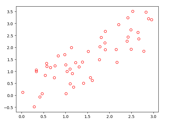
45 |
46 | 降维后数据图像:
47 |
48 | 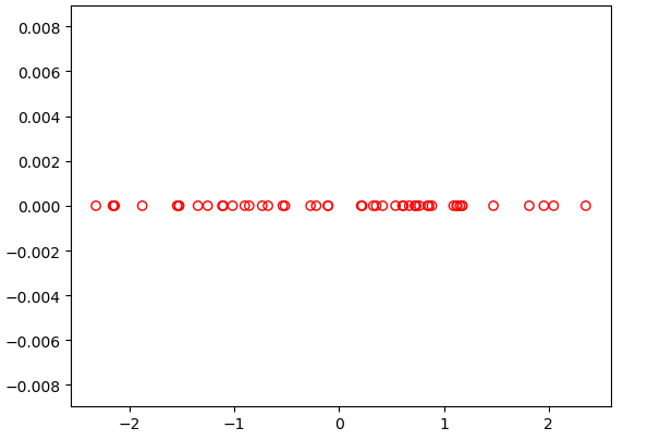
49 |
50 |
51 |
52 |
53 | ### 技术博客地址
54 |
55 | * [PCA(主成分分析-principal components analysis)学习笔记以及源代码实战讲解](https://blog.csdn.net/lzx159951/article/details/105912705)
56 |
57 |
--------------------------------------------------------------------------------
/决策树/datasets/lenses.txt:
--------------------------------------------------------------------------------
1 | young myope no reduced no lenses
2 | young myope no normal soft
3 | young myope yes reduced no lenses
4 | young myope yes normal hard
5 | young hyper no reduced no lenses
6 | young hyper no normal soft
7 | young hyper yes reduced no lenses
8 | young hyper yes normal hard
9 | pre myope no reduced no lenses
10 | pre myope no normal soft
11 | pre myope yes reduced no lenses
12 | pre myope yes normal hard
13 | pre hyper no reduced no lenses
14 | pre hyper no normal soft
15 | pre hyper yes reduced no lenses
16 | pre hyper yes normal no lenses
17 | presbyopic myope no reduced no lenses
18 | presbyopic myope no normal no lenses
19 | presbyopic myope yes reduced no lenses
20 | presbyopic myope yes normal hard
21 | presbyopic hyper no reduced no lenses
22 | presbyopic hyper no normal soft
23 | presbyopic hyper yes reduced no lenses
24 | presbyopic hyper yes normal no lenses
--------------------------------------------------------------------------------
/微信读书答题辅助/README.md:
--------------------------------------------------------------------------------
1 | ## 微信读书答题辅助python小程序
2 |
3 |
4 | ### 依赖环境
5 |
6 | python3.7
7 |
8 | ### python库
9 |
10 | * urllib
11 | * Pillow
12 | * BeautifulSoup4
13 | * base64
14 | * requests
15 | * time
16 | * re
17 |
18 |
19 | ### 下载安装
20 |
21 | ```
22 | git clone https://github.com/lzx1019056432/Be-Friendly-To-New-People.git
23 | ```
24 |
25 | ### 安装依赖包
26 |
27 | ```
28 | cd 微信读书答题辅助
29 | pip install -r requirements.txt
30 | ```
31 |
32 | ### 使用方法
33 |
34 | 在当前目录下输入
35 |
36 | ```
37 | cd 微信读书答题辅助
38 | ```
39 |
40 | 运行程序
41 |
42 | ```
43 | python question-answer.py
44 | ```
45 |
46 | ### 效果图
47 | 答题图:
48 |
49 | 
50 |
51 |
52 | ### 注意事项:
53 |
54 | 1. 使用前请查看技术文档
55 | 2. 不想修改截图位置的话,请将mumu模拟器放在屏幕左上角
56 |
57 |
58 | ### 技术博客地址
59 |
60 | * [从0到1使用python开发一个半自动答题小程序](https://blog.csdn.net/lzx159951/article/details/106062579)
61 |
62 |
--------------------------------------------------------------------------------
/Building-NN-model-with-numpy/README.md:
--------------------------------------------------------------------------------
1 | > # 此项目百度深度学习课程中的一个例子,使用numpy搭建一个神经网络
2 |
3 |
4 |
5 | ## 项目说明
6 |
7 | 1. 此项目来源于百度深度学习课程中的一个实例。课程链接:[百度架构师手把手教深度学习](https://aistudio.baidu.com/aistudio/education/group/info/888)
8 | 2. 本节课程是以notebook文档的形式,全文大概13000字所有,并配有详细的图文和代码说明,只要你有一些python和numpy的基础,一定能看的明明白白的。
9 | 3. 项目中的reference.md文件就是课程中的文档,图片outputxx.png是文档inference.md中的图片
10 | 4. 由于github对无法很好的显示数学公式,大家可以去博客查看文档 [博客地址](https://blog.csdn.net/lzx159951/article/details/105071799)
11 |
12 |
13 |
14 | ## 项目运行
15 |
16 | 1. 安装python3.7
17 | 2. 安装numpy 1.16 及以上
18 | 3. 编辑器推荐pycharm
19 | 4. data 文件夹是数据所在文件、combat1.py 是使用梯度下降法的神经网络项目,combat1-SGD.py 是改良后的随机梯度下降法的神经网络项目
20 | 5. combat2-onehidden.py文件是手写三层神经网络模型,搭配的博客地址为:[python和numpy纯手写3层神经网络,干货满满](https://blog.csdn.net/lzx159951/article/details/105099166)
21 |
22 |
23 |
24 | ## 闲话
25 |
26 | 不得不说,这个**手动搭建神经网络教程** 是我见过讲的最好的一个教程,没有之一,相信大家完整的看完之后,一定会有很大收获。对了,文档最下面还有一些小作业,大家可以去思考一下🙂
27 |
28 |
--------------------------------------------------------------------------------
/基于单层决策树的AdaBoost算法/README.md:
--------------------------------------------------------------------------------
1 | ## 基于单层决策树的AdaBoost算法
2 |
3 |
4 | ### 依赖环境
5 |
6 | python3.7
7 |
8 | ### python库
9 |
10 | numpy
11 |
12 | ### 下载安装
13 |
14 | ```
15 | git clone https://github.com/lzx1019056432/Be-Friendly-To-New-People.git
16 | ```
17 |
18 | ### 安装依赖包
19 |
20 | ```
21 | cd 基于单层决策树的AdaBoost算法
22 | pip install -r requirements.txt
23 | ```
24 | ### 文件介绍
25 | * datasets 为数据文件
26 | * 基于单层决策树的AdaBoost.py 为决策树主函数文件
27 |
28 |
29 | ### 使用方法
30 |
31 | 在当前目录下输入
32 |
33 | ```
34 | cd 基于单层决策树的AdaBoost算法
35 | ```
36 |
37 | 运行AdaBoost算法
38 |
39 | ```
40 | python 基于单层决策树的AdaBoost.py
41 | ```
42 |
43 | ## 获取的最佳分类决策树:
44 | [{'dim': 0, 'thresh': 4.5301945, 'ineq': 'lt', 'alpha': 2.1847239262335107},
45 | {'dim': 0, 'thresh': 5.5848406, 'ineq': 'lt', 'alpha': 2.528122902674154},
46 | {'dim': 1, 'thresh': -1.8740486000000005, 'ineq': 'gt', 'alpha': 1.0220510876172635}]
47 |
48 |
49 |
50 | ### 技术博客地址
51 |
52 | * [决策树代码实战](https://blog.csdn.net/lzx159951/article/details/106809994)
53 |
54 |
--------------------------------------------------------------------------------
/决策树/README.md:
--------------------------------------------------------------------------------
1 | ## 决策树代码
2 |
3 |
4 | ### 依赖环境
5 |
6 | python3.7
7 |
8 | ### python库
9 |
10 | numpy
11 |
12 | matplotlib
13 |
14 | ### 下载安装
15 |
16 | ```
17 | git clone https://github.com/lzx1019056432/Be-Friendly-To-New-People.git
18 | ```
19 |
20 | ### 安装依赖包
21 |
22 | ```
23 | cd 决策树
24 | pip install -r requirements.txt
25 | ```
26 | ### 文件介绍
27 | * datasets 为数据文件
28 | * decision-tree.py 为决策树主函数文件
29 | * treePlotter.py 使用matplotlib绘画决策树
30 |
31 | ### 使用方法
32 |
33 | 在当前目录下输入
34 |
35 | ```
36 | cd 决策树
37 | ```
38 |
39 | 运行决策树算法
40 |
41 | ```
42 | python decision-tree.py
43 | ```
44 |
45 | ## 决策树格式
46 |
47 | 决策树产生字典的字典形式为:
48 |
49 | ```
50 | {'tearRate': {'reduced': 'no lenses', 'normal': {'astigmatic': {'no': {'age': {'presbyopic': {'prescript': {'hyper': 'soft', 'myope': 'no lenses'}}, 'young': 'soft', 'pre': 'soft'}}, 'yes': {'prescript': {'hyper': {'age': {'presbyopic': 'no lenses', 'young': 'hard', 'pre': 'no lenses'}}, 'myope': 'hard'}}}}}}
51 | ```
52 |
53 | 决策树图形表示:
54 |
55 | 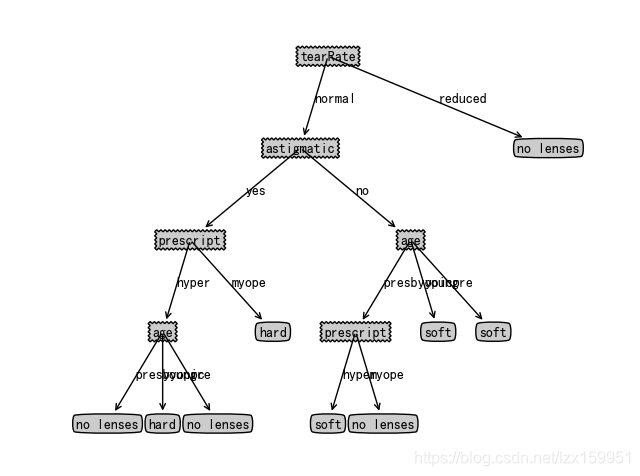
56 |
57 | ### 技术博客地址
58 |
59 | * [决策树代码实战](https://blog.csdn.net/lzx159951/article/details/106172243)
60 |
61 |
--------------------------------------------------------------------------------
/GeneratorGIF-and-SeparateGIF/SeparateGif.py:
--------------------------------------------------------------------------------
1 | from PIL import Image
2 | import numpy as np
3 | import imageio
4 | import argparse
5 | import os
6 | '''
7 | 作者:@梁先森
8 | CSDN博客地址:https://blog.csdn.net/lzx159951
9 | github地址:
10 | 实现功能:将gif分离成一张张图片
11 | '''
12 |
13 | parser = argparse.ArgumentParser()
14 | parser.add_argument("-i",type=str,default="image",help="Please input GIF picture")
15 | parser.add_argument("-o","-output",default="outputimage",type=str,help="the name of output image")
16 | args = parser.parse_args()
17 | try:
18 | imagelist = imageio.mimread(args.i)
19 | print("GIF文件已成功读取")
20 | except:
21 | print("GIF文件读取失败")
22 | num=-1
23 | path=''
24 | try:
25 | if(not os.path.exists('output')):
26 | os.mkdir('output')
27 | path = 'output/'
28 | for i in imagelist:
29 | num+=1
30 | im = Image.fromarray(i)
31 | imagearray = np.array(i)
32 | if(imagearray.shape[2]==4):
33 | if(str(args.o).lower().endswith('.jpg') or str(args.o).lower().endswith('.jpeg') or str(args.o).lower().endswith('.png')):
34 | output = path+str(args.o).split('.')[0]+str(num)+'.png'
35 | else:
36 | output = path+str(args.o)+str(num)+'.png'
37 | imageio.imwrite(output,imagearray)
38 | print("GIF图片分离成功")
39 | except:
40 | print("GIF图片分离失败")
41 |
42 |
--------------------------------------------------------------------------------
/GeneratorGIF-and-SeparateGIF/README.md:
--------------------------------------------------------------------------------
1 | ## GeneratorGIF-and-SeparateGIF
2 | 此项目是GIF图片的生成和GIF图片的分离。
3 |
4 | 
5 |
6 | 生成样例图
7 |
8 | ### 依赖环境
9 |
10 | python 3.7
11 |
12 | ### python 库
13 |
14 | numpy--图片格式操作
15 |
16 | pillow--图片操作
17 |
18 | imageio--图片相关操作
19 |
20 | os-- 文件路径操作
21 |
22 | argparse--命令行参数处理
23 |
24 | ### 下载安装
25 |
26 | ```
27 | git clone https://github.com/lzx1019056432/Be-Friendly-To-New-People.git
28 | ```
29 |
30 | ### 安装依赖包
31 |
32 | ```
33 | pip install -r requirements.txt
34 | ```
35 |
36 | ### 使用方式
37 |
38 | 在当前目录下输入:
39 |
40 | ```
41 | cd GeneratorGIF-and-SeparateGIF
42 | ```
43 |
44 | 第一次在GitHub上整理资源,有哪些做的不恰当的地方,还希望各位大佬多提提意见。做这个的初心就是想收集一些比较好的机器学习和人工智能入门案例,带有详细文档解释。这样也大大降低入门门槛,同时减少了新手各种找资料的实践。如果有愿意一起完善这个项目的,可以邮箱联系我 1019056432 @qq.com 期待与大佬一起做一件有意义的事。
45 |
46 | * 生成GIF图片
47 |
48 | ```
49 | python GeneratorGif.py -i image -o outputimage -d 0.5
50 | ```
51 |
52 | -i 后面需跟上图片所在的文件夹
53 |
54 | -o 输出的图片名称
55 |
56 | -d GIF图片播放速度,即每张图片转换延迟
57 |
58 | * 分解GIF图片
59 |
60 | ```
61 | python SeparateGif.py -i image.gif -o outputimage
62 | ```
63 |
64 | -i 后面添加需要分解的GIF图片
65 |
66 | -o 输出图片的名称,多图片后面使用递增数字区分
67 |
68 | ### 注释
69 |
70 | 1. 建议将需要合成的图片放到一个文件夹中,然后将文件放入GeneratorGIF-and-SeparateGIF目录下
71 | 2. 也可以将项目目录添加到系统环境变量中,这样就可以随时随地使用这个工具了。
72 | 3. 如果有任何疑问,欢迎大家CSDN私信我吗,我会第一时间给大家回答的。
--------------------------------------------------------------------------------
/GeneratorGIF-and-SeparateGIF/GeneratorGif.py:
--------------------------------------------------------------------------------
1 | from PIL import Image
2 | import numpy as np
3 | import imageio
4 | import argparse
5 | import os
6 | '''
7 | 作者:@梁先森
8 | CSDN博客地址:https://blog.csdn.net/lzx159951
9 | 实现功能:实现图片转换成gif、分离gif为图片
10 |
11 | '''
12 | parser = argparse.ArgumentParser()
13 | parser.add_argument("-i",type=str,default="image",help="Please input the file folder path of the picture")
14 | parser.add_argument("-o","-output",default="outputimage",type=str,help="the name of output image")
15 | parser.add_argument("-d",default="0.5",type=float,help="Picture playback interval")
16 |
17 | args = parser.parse_args()
18 | listimage=[]#存储图片
19 | listname=[]#存储图片地址
20 | try:
21 | if(not os.path.exists(args.i)):
22 | print("您输入的文件夹地址或者图片地址不存在!")
23 | else:
24 | for imagename in os.listdir('image'):
25 | if(imagename.lower().endswith('jpg') or imagename.lower().endswith('png')):
26 | listname.append(imagename)
27 | print("读取图片完成")
28 | for imagename in listname:
29 | if imagename.find('.'):
30 | im = Image.open(args.i+'/'+imagename)
31 | im = np.array(im)
32 | listimage.append(im)
33 | #创建文件夹
34 | if(not os.path.exists(args.i+'/output')):
35 | os.mkdir(args.i+'/output')
36 | if(str(args.o).lower().endswith('.gif')):
37 | filename=args.i+'/output/'+args.o
38 | else:
39 | filename = args.i+'/output/'+args.o+'.gif'
40 | print("正在生成gif......")
41 | imageio.mimsave(filename,listimage,'GIF',duration=args.d)
42 | print("gif输出完毕,感谢使用")
43 | except:
44 | print("图片转换失败")
--------------------------------------------------------------------------------
/SVM支持向量机/.idea/workspace.xml:
--------------------------------------------------------------------------------
1 |
2 |
3 |
4 |
5 |
6 |
7 |
8 |
9 |
10 |
11 |
12 |
13 |
14 |
15 |
16 |
17 |
18 |
19 |
20 |
21 |
22 |
23 |
24 |
25 |
26 |
27 |
28 |
29 |
30 |
31 |
32 |
33 |
34 |
35 |
37 |
38 |
39 |
--------------------------------------------------------------------------------
/PCA/PCA.py:
--------------------------------------------------------------------------------
1 | # -*- coding:utf-8 -*-
2 | '''
3 | PCA 主成分分析
4 | 步骤:
5 | 1.将原始数据按列组成n行m列矩阵X
6 | 2. 将X的每一行进行零均值化,即减去这一行的值
7 | 3.求出协方差矩阵C=1/mXXT
8 | 4. 求出协方差矩阵的特征值及对应的特征向量
9 | 5. 将特征向量按对应特征值大小从上到下按行排成矩阵,取前K行组成矩阵P
10 | 6. Y=PX即为降维到K维后的数据
11 |
12 | 注:
13 | 这里的数据格式为 行代表数据,列代表属性。这个与之前看的资料正好相反,不过影响不大。
14 | '''
15 | import numpy as np
16 | import matplotlib.pyplot as plt
17 | #加载数据,输出为矩阵形式
18 | def loadDateSet(filename,delim='\t'):
19 | with open(filename,'r')as f:
20 | stringarr = [line.strip().split(delim) for line in f.readlines()]
21 | datarr = [list(map(float,line)) for line in stringarr]
22 | return np.mat(datarr)
23 |
24 | def pca(dataMat,topNfeat=999):
25 | meanVals = np.mean(dataMat,axis=0)#计算每一个属性的均值
26 | meanRemoved = dataMat-meanVals#将数据进行零均值化
27 | covMat = np.cov(meanRemoved,rowvar=False)#计算协方差矩阵,rowvar=False 表示属性在列,数据在行
28 | eigVals,eigVects = np.linalg.eig(np.mat(covMat))#计算矩阵的特征值和特征向量
29 | #print("特征值:",eigVals)
30 | #print("特征向量:",eigVects)
31 | eigValInd = np.argsort(eigVals)#将特征值进行排序,按照从小到大的顺序,返回索引值
32 | #print("排序后的特征值:",eigValInd)
33 | #这里就是取前K个最大值
34 | eigValInd = eigValInd[:-(topNfeat+1):-1] #这里使用了切片,只取前K个最大的索引,这里我们K=1
35 | #print("eigValInd:",eigValInd)
36 | redEigVects = eigVects[:,eigValInd] #取特征值对应的特征向量
37 | #print("redEigVects",redEigVects)
38 | #Y=XP
39 | lowDDataMat = meanRemoved*redEigVects #零均值的数据与 特征向量做相乘 结果为Y,降维后的数据
40 | #redEigVects.T 为对redEigVects 进行转置
41 | #这里为何能还原呢,是因为P是特征向量,特征向量P*其转置=E so XP*PT=X
42 | reconMat = (lowDDataMat*redEigVects.T)+meanVals #数据还原
43 | return lowDDataMat,reconMat
44 |
45 | if __name__ == '__main__':
46 | datamat = loadDateSet('data.txt')
47 | lowDDataMat,reconmat = pca(datamat,1)
48 | print("原数据:\n",reconmat)
49 | print("降维后的数据:\n",lowDDataMat)
--------------------------------------------------------------------------------
/LineRegression/LineRegression.py:
--------------------------------------------------------------------------------
1 | # -*- coding:utf-8 -*-
2 | '''
3 | 参考《机器学习实战》
4 | 使用最小二乘法算法进行求解问题
5 |
6 | '''
7 |
8 | import numpy as np
9 | import matplotlib.pyplot as plt
10 | def LoadData(filename):
11 | dataMat = []
12 | labelMat = []
13 | with open(filename) as f:
14 | numFeat = len(f.readline().split('\t'))-1#这里会导致忽略第一个数据
15 | for line in f.readlines():
16 | lineArr = []
17 | curLine = line.strip().split('\t')
18 | for i in range(numFeat):
19 | lineArr.append(float(curLine[i]))
20 | dataMat.append(lineArr)
21 | labelMat.append(float(curLine[-1]))
22 | return dataMat,labelMat
23 | def standRegres(xArr,yArr):
24 | xMat = np.mat(xArr);yMat = np.mat(yArr).T#由于原来形状是(1,199),所以这里需要转置
25 | print("yMat",yMat.shape)#yMat (199, 1)
26 | xTx = xMat.T*xMat
27 | if np.linalg.det(xTx)==0.0:
28 | print("false")
29 | return
30 | print("xtx.shape",xTx.shape)#形状:(2,2)
31 | print("xTx.I",xTx.I)#矩阵的逆
32 | print("xMat.T",(xMat.T).shape)
33 | ws = xTx.I*(xMat.T*yMat)#(xMat.T*yMat)形状为(2,1)
34 | return ws
35 |
36 | def showdata(xArr,yMat,ws):
37 | fig = plt.figure()
38 | ax = fig.add_subplot(111)
39 | xCopy = xArr.copy()
40 | xCopy.sort(0)
41 | yHat = xCopy*ws
42 | ax.scatter(xArr[:,1].flatten().tolist(),yMat.T[:,0].flatten().tolist(),s=20,alpha=0.5)
43 | ax.plot(xCopy[:,1],yHat)
44 | plt.show()
45 | def pearsoncor(yHat,yMat):
46 | result = np.corrcoef(yHat.T,yMat)#相关系数分析。越接近1,表示相似度越高
47 | print("pearson-result:",result)
48 |
49 |
50 | if __name__ == '__main__':
51 | xArr,yArr = LoadData('datasets/ex0.txt')
52 | print(xArr)
53 | ws = standRegres(xArr,yArr)
54 | print("ws:",ws)#输出w
55 | xMat = np.mat(xArr)
56 | yMat = np.mat(yArr)
57 | yHat = xMat*ws#获得预测值
58 | showdata(xMat,yMat,ws)#图像显示
59 | pearsoncor(yHat,yMat)#进行相关度分析
60 | print("yArr[0]",yArr[0])
61 |
62 |
--------------------------------------------------------------------------------
/PCA/data.txt:
--------------------------------------------------------------------------------
1 | 1.0089380119044606 1.2656678128352157
2 | 1.3112528199132147 1.1807446761302725
3 | 2.424508865890327 2.42623813185137
4 | 1.0147525857585666 0.06368262131662794
5 | 1.1578567759128777 0.9024219166888485
6 | 0.5722916129482798 1.3253794224645534
7 | 0.2908871361168006 -0.48463308082989065
8 | 1.1053724904864857 1.0911672155623187
9 | 2.782643175630093 1.8344774809236917
10 | 1.1371327811239178 1.9855014728748523
11 | 2.9595202573961683 3.1493568304265667
12 | 0.03001377099248237 0.1184138168692801
13 | 1.6105626276842764 0.6151813024295321
14 | 2.40192019049226 2.2532532683638085
15 | 1.0377638875699935 0.9891452647051595
16 | 1.9068506322033905 2.6633954432208444
17 | 2.8902965567858003 3.190505116006065
18 | 1.387127300556284 1.3822077284377672
19 | 2.1723405537093683 1.3703297004736115
20 | 1.1082474794834063 0.476093034988174
21 | 2.832791781368075 3.465027202868262
22 | 1.2329543292136673 1.3580114948781103
23 | 0.3383435782654256 1.0496994597605154
24 | 2.6686732678308283 2.3496745526652143
25 | 2.154185375024965 1.905677081834225
26 | 1.4121985566741515 0.4981343973255359
27 | 0.9851509398902834 1.6913204917122577
28 | 1.568840906349229 0.7314958832099767
29 | 2.2116472577644415 2.9455247453019044
30 | 2.494869052708789 1.9164818029038488
31 | 1.8139006367300752 2.408621604326571
32 | 1.773479929898689 1.4804511173353605
33 | 0.7635093683671226 1.2246723892862486
34 | 0.41923787374006094 -0.07487849240816102
35 | 0.5411773173213034 0.8263056748482267
36 | 0.8364437773383608 1.6408482378736724
37 | 2.4892980267068867 2.727527588160629
38 | 0.7481168620570725 0.72830031282616
39 | 0.3392311809900582 0.9855980245973939
40 | 0.5786230011762762 1.2000957680538957
41 | 1.9067969026591851 1.897918445903974
42 | 0.6608553944889943 1.1524725820678174
43 | 1.7850248331657892 2.0217406020350204
44 | 2.6498704423269475 2.6190156209335624
45 | 1.1854548209066529 0.3359742053709607
46 | 0.4713755383568643 0.06201732243202529
47 | 1.8982073515313658 2.1822442745683635
48 | 2.419962189930445 3.230103406395937
49 | 1.5197960108303117 1.8251570655193818
50 | 2.5304157468853683 3.499657694315162
51 |
--------------------------------------------------------------------------------
/K-mean/data.txt:
--------------------------------------------------------------------------------
1 | 1.0089380119044606 1.2656678128352157
2 | 1.3112528199132147 1.1807446761302725
3 | 2.424508865890327 2.42623813185137
4 | 1.0147525857585666 0.06368262131662794
5 | 1.1578567759128777 0.9024219166888485
6 | 0.5722916129482798 1.3253794224645534
7 | 0.2908871361168006 -0.48463308082989065
8 | 1.1053724904864857 1.0911672155623187
9 | 2.782643175630093 1.8344774809236917
10 | 1.1371327811239178 1.9855014728748523
11 | 2.9595202573961683 3.1493568304265667
12 | 0.03001377099248237 0.1184138168692801
13 | 1.6105626276842764 0.6151813024295321
14 | 2.40192019049226 2.2532532683638085
15 | 1.0377638875699935 0.9891452647051595
16 | 1.9068506322033905 2.6633954432208444
17 | 2.8902965567858003 3.190505116006065
18 | 1.387127300556284 1.3822077284377672
19 | 2.1723405537093683 1.3703297004736115
20 | 1.1082474794834063 0.476093034988174
21 | 2.832791781368075 3.465027202868262
22 | 1.2329543292136673 1.3580114948781103
23 | 0.3383435782654256 1.0496994597605154
24 | 2.6686732678308283 2.3496745526652143
25 | 2.154185375024965 1.905677081834225
26 | 1.4121985566741515 0.4981343973255359
27 | 0.9851509398902834 1.6913204917122577
28 | 1.568840906349229 0.7314958832099767
29 | 2.2116472577644415 2.9455247453019044
30 | 2.494869052708789 1.9164818029038488
31 | 1.8139006367300752 2.408621604326571
32 | 1.773479929898689 1.4804511173353605
33 | 0.7635093683671226 1.2246723892862486
34 | 0.41923787374006094 -0.07487849240816102
35 | 0.5411773173213034 0.8263056748482267
36 | 0.8364437773383608 1.6408482378736724
37 | 2.4892980267068867 2.727527588160629
38 | 0.7481168620570725 0.72830031282616
39 | 0.3392311809900582 0.9855980245973939
40 | 0.5786230011762762 1.2000957680538957
41 | 1.9067969026591851 1.897918445903974
42 | 0.6608553944889943 1.1524725820678174
43 | 1.7850248331657892 2.0217406020350204
44 | 2.6498704423269475 2.6190156209335624
45 | 1.1854548209066529 0.3359742053709607
46 | 0.4713755383568643 0.06201732243202529
47 | 1.8982073515313658 2.1822442745683635
48 | 2.419962189930445 3.230103406395937
49 | 1.5197960108303117 1.8251570655193818
50 | 2.5304157468853683 3.499657694315162
51 |
--------------------------------------------------------------------------------
/ROC曲线和AUC面积/ROC-AUC.py:
--------------------------------------------------------------------------------
1 | # -*- coding:utf-8 -*-
2 | import numpy as np
3 | import matplotlib.pyplot as plt
4 | def loadSimpData():
5 | dataMat = []
6 | labelMat = []
7 | data = open('datasets/testSet.txt')
8 | for dataline in data.readlines():
9 | linedata = dataline.split('\t')
10 | dataMat.append([float(linedata[0]),float(linedata[1])])
11 | labelMat.append(float(linedata[2].replace('\n','')))
12 | return dataMat,labelMat
13 |
14 | def plotROC(predStrengths,classLabels):
15 | #predStrengths = np.fabs(predStrengths)
16 | # print("predStrengths:",predStrengths[0])
17 | # print("sorted(predStrengths):",sorted(list(predStrengths[0])))
18 | cur = (0.0,0.0)
19 | ySum = 0.0
20 | numPosClas = np.sum(np.array(classLabels)==1.0)
21 | yStep = 1/float(numPosClas)
22 | xStep = 1/float(len(classLabels)-numPosClas)
23 | sortedIndicies = list(predStrengths.argsort())
24 | sortedIndicies.sort(reverse=True)
25 | fig = plt.figure()
26 | fig.clf()
27 | ax = fig.add_subplot(111)
28 | for index in sortedIndicies:
29 | if classLabels[index]==1:
30 | addX = 0
31 | addY = yStep
32 | else:
33 | addX = xStep
34 | addY=0
35 | ySum+=cur[1]
36 | # print("[cur[0],cur[0]-delX]:",[cur[0],cur[0]-delX])
37 | # print("[cur[1],cur[1]-delY]:",[cur[1],cur[1]-delY])
38 | ax.plot([cur[0],cur[0]+addX],[cur[1],cur[1]+addY],c='r')#[1,1],[1,]
39 | print("ystep,xstep",yStep,xStep)
40 | cur = (cur[0]+addX,cur[1]+addY)
41 | ax.plot([0,1],[0,1],'b--')
42 | plt.xlabel('False Positive Rate')
43 | plt.ylabel('True Positive Rate')
44 | plt.title('Roc curve for AdaBoost Horse Colic Detection System')
45 | #ax.axis([0,1,0,1])
46 | plt.show()
47 | print('the Area Under the Curve is :',ySum*xStep)
48 |
49 | if __name__ == '__main__':
50 | dataMat,classLabels = loadSimpData()
51 | traindata = np.mat(dataMat[:80]);trainclasslabels = np.array(classLabels[:80])
52 | predStrengths = np.array([i/10 for i in range(1,80)])
53 | plotROC(predStrengths,trainclasslabels)
54 |
55 |
--------------------------------------------------------------------------------
/LwLineReg/LwLineReg.py:
--------------------------------------------------------------------------------
1 | # -*- coding:utf-8 -*-
2 |
3 | '''
4 | 局部加权线性回归算法
5 |
6 | '''
7 | import numpy as np
8 | import matplotlib.pyplot as plt
9 | def LoadData(filename):
10 | dataMat = []
11 | labelMat = []
12 | with open(filename) as f:
13 | numFeat = len(f.readline().split('\t'))-1#这里会导致忽略第一个数据
14 | f.seek(0)
15 | for line in f.readlines():
16 | lineArr = []
17 | curLine = line.strip().split('\t')
18 | for i in range(numFeat):
19 | lineArr.append(float(curLine[i]))
20 | dataMat.append(lineArr)
21 | labelMat.append(float(curLine[-1]))
22 | return dataMat,labelMat
23 |
24 | #局部加权线性回归
25 | def lwlr(testPoint,xArr,yArr,k=0.1):
26 | xMat = np.mat(xArr);yMat = np.mat(yArr).T#
27 | m = np.shape(xMat)[0]#数据个数
28 | #为什么创建方阵,是为了实现给每个数据增添不同的权值
29 | weights = np.mat(np.eye(m))#初始化一个阶数等于m的方阵,其对角线的值为1,其余值均为0
30 | for j in range(m):
31 | diffMat = testPoint-xMat[j,:]
32 | weights[j,j] = np.exp(diffMat*diffMat.T/(-2.0*k**2)) #e的指数形式
33 | xTx = xMat.T*(weights*xMat)
34 | #print("weights",weights)
35 | if np.linalg.det(xTx)==0.0:#通过计算行列式的值来判是否可逆
36 | print("this matrix is singular,cannot do inverse")
37 | return
38 | ws = xTx.I*(xMat.T*(weights*yMat))
39 | return testPoint*ws
40 | def lwlrTest(testArr,xArr,yArr,k=1.0):
41 | m = np.shape(testArr)[0]
42 | yHat = np.zeros(m)
43 | for i in range(m):
44 | yHat[i] = lwlr(testArr[i],xArr,yArr,k)
45 | return yHat
46 | #图像显示
47 | def lwlshow(xArr,yMat,yHat,k):
48 | fig = plt.figure()
49 | ax = fig.add_subplot(111)
50 | xCopy = np.array(xArr.copy())
51 | srtInd = xCopy[:,1].argsort(0)
52 | print("xSort",xCopy[srtInd])
53 | ax.plot(xCopy[srtInd][:,1],yHat[srtInd])
54 | yMat = np.array(yMat)
55 | ax.scatter(xCopy[srtInd][:,1].tolist(),yMat[srtInd],s=10,alpha=0.7)
56 | ax.set_title("k={}".format(str(k)))
57 | plt.show()
58 | if __name__ == '__main__':
59 | xArr,yArr = LoadData('datasets/ex0.txt')
60 | ytest = lwlr(xArr[0],xArr,yArr,1.0)
61 | print("xArr[0],ytest",xArr[0],ytest)
62 | k=0.01
63 | yHat = lwlrTest(xArr,xArr,yArr,k)
64 | lwlshow(xArr,yArr,yHat,k)
--------------------------------------------------------------------------------
/forward-regression/forward-regression.py:
--------------------------------------------------------------------------------
1 | # -*- coding:utf-8 -*-
2 | '''
3 | 前向逐步线性回归
4 |
5 |
6 | '''
7 | import numpy as np
8 | import matplotlib.pyplot as plt
9 |
10 | plt.rcParams['font.sans-serif']=['SimHei']#这两句作用为防止中文乱码
11 | plt.rcParams['axes.unicode_minus']=False
12 | #加载数据
13 | def LoadData(filename):
14 | dataMat = []
15 | labelMat = []
16 | with open(filename) as f:
17 | numFeat = len(f.readline().split('\t'))-1#这里会导致忽略第一个数据
18 | f.seek(0)
19 | for line in f.readlines():
20 | lineArr = []
21 | curLine = line.strip().split('\t')
22 | for i in range(numFeat):
23 | lineArr.append(float(curLine[i]))
24 | dataMat.append(lineArr)
25 | labelMat.append(float(curLine[-1]))
26 | return dataMat,labelMat
27 |
28 | ## 损失值计算
29 | def rssError(yMat,yTest):
30 | result = np.sum(np.power((yMat-yTest),2),0)
31 | return result
32 |
33 | def stageWise(xArr,yArr,eps=0.01,numIt=300):
34 | xMat = np.mat(xArr);yMat = np.mat(yArr).T
35 | yMean = np.mean(yMat,0)
36 | # 数据标准化
37 | xMean = np.mean(xMat,0)
38 | yMat = yMat-yMean
39 | xVar = np.var(xMat,0)
40 | xMat = (xMat-xMean)/xVar
41 | #
42 | m,n = np.shape(xMat)
43 | returnMat = np.zeros((numIt,n))
44 | ws = np.zeros((n,1));wsTest = ws.copy();wsMax = ws.copy()
45 | for i in range(numIt):
46 | lowestError = np.power(10,5)#初始化一个最大值
47 | for j in range(n):
48 | for sign in [-1,1]:
49 | wsTest = ws.copy()
50 | wsTest[j]+=eps*sign
51 | yTest = xMat*wsTest
52 | rssE = rssError(yMat.A,yTest.A)
53 | #print("rssE:",rssE)
54 | if rssE0.5]=1
48 | h[h<0.5]=0
49 | result = h
50 | error=0
51 | for i in range(len(result)):
52 | if(result[i]!=y[i]):
53 | error+=1
54 | print(" the error is {}%:".format(100*error/float(len(result))))
55 |
56 | def showimg(self,dataset,i):
57 | x = np.arange(-3.0,3.0,0.1)
58 | x2 = (-self.w[0]-x*self.w[1])/self.w[2]
59 | plt.scatter([dataset[dataset[:,-1]==0][:,1]],[dataset[dataset[:,-1]==0][:,2]],color='',marker='o',edgecolors='green',linewidths=3)
60 | plt.scatter([dataset[dataset[:,-1]==1][:,1]],[dataset[dataset[:,-1]==1][:,2]],color='',marker='o',edgecolors='red',linewidths=3)
61 | plt.plot(x,x2)
62 | plt.title("迭代第{}次".format(i))
63 | # plt.savefig('datasets/img{}.png'.format(i))
64 | plt.show()
65 |
66 | if __name__ == '__main__':
67 | filename="datasets/logisticdata.txt"
68 | dataset = loaddata(filename)
69 | print(np.shape(dataset))
70 | traindata = dataset[:80]
71 | testdata = dataset[80:]
72 | print(len(traindata))
73 | logistic = Logistic()
74 | logistic.train(dataset,epoch=500)
75 | logistic.test(testdata)
76 | # logistic.showimg(dataset)
77 |
--------------------------------------------------------------------------------
/README.md:
--------------------------------------------------------------------------------
1 | # Be-Friendly-To-New-People
2 | 此项目是一些机器学习和人工智能的项目实战,每一个文件夹都是一个具体的实战项目,目的就是让新人能够快速动手实践,延续学习的热情!
3 |
4 | ## 项目列表
5 |
6 | | 序号 | 文件名 | 项目简述 | 项目地址 |
7 | | :--: | :----------------------------: | :------------------------------: | :----------------------------------------------------------: |
8 | | 1 | [Building-NN-model-with-numpy] | 使用numpy手写神经网络(2层和3层) | [项目地址](https://github.com/lzx1019056432/Be-Friendly-To-New-People/tree/master/Building-NN-model-with-numpy) |
9 | | 2 | [GeneratorGIF-and-SeparateGIF] | 实现多个图片转GIF和GIF分离 | [项目地址](https://github.com/lzx1019056432/Be-Friendly-To-New-People/tree/master/GeneratorGIF-and-SeparateGIF) |
10 | | 3 | [K-mean] | K-mean算法源代码实现以及详细注释 | [项目地址](https://github.com/lzx1019056432/Be-Friendly-To-New-People/tree/master/K-mean) |
11 | | 4 | [PCA] | 主成分分析源代码实现以及详细注释 | [项目地址](https://github.com/lzx1019056432/Be-Friendly-To-New-People/tree/master/PCA) |
12 | | 5 | [微信读书答题辅助] |python代码实现微信读书每日答题答题半自动化 | [项目地址](https://github.com/lzx1019056432/Be-Friendly-To-New-People/tree/master/%E5%BE%AE%E4%BF%A1%E8%AF%BB%E4%B9%A6%E7%AD%94%E9%A2%98%E8%BE%85%E5%8A%A9) |
13 | | 6 | [KNN] | k-邻近算法源代码以及详细注解 | [项目地址](https://github.com/lzx1019056432/Be-Friendly-To-New-People/tree/master/KNN) |
14 | | 7 | [决策树] | 决策树算法的原理分析和代码详解 | [项目地址](https://github.com/lzx1019056432/Be-Friendly-To-New-People/tree/master/%E5%86%B3%E7%AD%96%E6%A0%91) |
15 | | 8 | [朴素贝叶斯] | 朴素贝叶斯原理分析和代码详解 | [项目地址](https://github.com/lzx1019056432/Be-Friendly-To-New-People/tree/master/朴素贝叶斯) |
16 | | 9 | [Logistic分类回归] | 逻辑回归分类算法分析和代码详解 | [项目地址](https://github.com/lzx1019056432/Be-Friendly-To-New-People/tree/master/Logistic回归算法) |
17 | | 10 | [SVM支持向量机] | SVM分类算法分析和代码详情 | [项目地址](https://github.com/lzx1019056432/Be-Friendly-To-New-People/tree/master/SVM支持向量机) |
18 | | 11 | [基于单层决策树的AdaBoost] | 基于单层决策树的AdaBoost算法分析和代码 | [项目地址](https://github.com/lzx1019056432/Be-Friendly-To-New-People/tree/master/基于单层决策树的AdaBoost算法) |
19 | | 12 | [ROC曲线和AUC面积] | ROC曲线原理分析和代码实战 | [项目地址](https://github.com/lzx1019056432/Be-Friendly-To-New-People/tree/master/ROC曲线和AUC面积) |
20 | | 13 | [LineRegression] | [基础线性回归算法原理以及项目实战] | [项目地址](https://github.com/lzx1019056432/Be-Friendly-To-New-People/tree/master/LineRegression) |
21 | | 14 | [LwLineReg] | [局部加权线性回归算法原理以及代码实战] | [项目地址](https://github.com/lzx1019056432/Be-Friendly-To-New-People/tree/master/LwLineReg) |
22 | | 15 | [ridge-regression] | [岭回归算法原理及代码实战] | [项目地址](https://github.com/lzx1019056432/Be-Friendly-To-New-People/tree/master/ridge-regression) |
23 | | 16 | [forward-regression] | [前向逐步线性回归算法原理及代码实战] | [项目地址](https://github.com/lzx1019056432/Be-Friendly-To-New-People/tree/master/forward-regression) |
24 |
25 |
26 |
27 | ## 闲话
28 |
29 | 第一次在GitHub上整理资源,有哪些做的不恰当的地方,还希望各位大佬多提提意见。做这个的初心就是想收集一些比较好的机器学习、人工智能、有趣的项目的入门案例,带有详细文档解释。这样也大大降低入门门槛,同时减少了新手各种找资料的时间。如果有愿意一起完善这个项目的,可以邮箱联系我 1019056432 @qq.com,或者通过下方的CSDN私信我期待与大佬一起做一件有意义的事。
30 | ### [CSDN主页地址](https://blog.csdn.net/lzx159951)
31 |
32 |
--------------------------------------------------------------------------------
/Building-NN-model-with-numpy/combat1.py:
--------------------------------------------------------------------------------
1 | import numpy as np
2 | import matplotlib.pyplot as plt
3 | '''
4 | 项目介绍:
5 | 此项目是使用numpy搭建神经网络模型,预测波士顿房价。
6 | 数据介绍:
7 | 每一条房屋数据有14个值,前13个值是房屋属性,比如面积,长度等,最后一个是房屋价格,共506条数据。
8 |
9 | '''
10 | #数据导入以及处理
11 | def deal_data():
12 | #读取文件数据,此时数据形状是(7084,),即所有数据在一行中
13 | housingdata = np.fromfile('data/housing.data',sep=' ')
14 |
15 | #修改数据格式,将每一条房屋数据放在一行中。
16 | housingdata = np.array(housingdata).reshape((-1,14))#此时数据形状为(506,14)
17 |
18 | #对数据的前13个属性进行归一化操作,有助于提高模型精准度,这里使用max-min归一化方式。公式为(x-min)/(max-min)
19 | for i in range(13):
20 | Max = np.max(housingdata[:,i])
21 | Min = np.min(housingdata[:,i])
22 | housingdata[:,i]=(housingdata[:,i]-Min)/(Max-Min)
23 |
24 | #依据2-8原则,80%的数据作为训练数据,20%数据作为测试数据;此时训练数据是405条,测试数据是101条
25 | Splitdata = round(len(housingdata)*0.8)
26 | Train = housingdata[:Splitdata]#训练数据集
27 | Test = housingdata[Splitdata:]#测试数据集
28 | return Train,Test
29 |
30 | #模型设计以及配置
31 | #首先确定有13个权值参数w,并随机初始化
32 | class Model_Config(object):
33 | def __init__(self,num):
34 | np.random.seed(1)
35 | self.w = np.random.randn(num,1)
36 | self.b =0
37 | #计算预测值
38 | def forward(self,x):
39 | y = np.dot(x,self.w)
40 | return y
41 | #设置损失函数,这里使用差平方损失函数计算方式
42 | def loss(self,z,y):
43 | error = z-y
44 | cost = error*error
45 | avg_cost = np.mean(cost)
46 | return avg_cost
47 | #计算梯度
48 | def back(self,x,y):
49 | z = self.forward(x)
50 | gradient_w = (z-y)*x
51 | gradient_w = np.mean(gradient_w,axis=0)#这里注意,axis=0必须写上,否则默认将这个数组变成一维的求平均
52 | gradient_w = gradient_w[:,np.newaxis]#这里注意写博客--增加一个维度
53 | gradient_b = (z-y)
54 | gradient_b = np.mean(gradient_b)
55 | return gradient_w,gradient_b
56 |
57 | #使用梯度更新权值参数w
58 | def update(self,gradient_w,gradient_b,learning_rate):
59 | self.w = self.w-learning_rate*gradient_w
60 | self.b = self.b-learning_rate*gradient_b
61 |
62 | #开始训练
63 | def train(self,epoch_num,x,y,learning_rate):
64 | #循环迭代
65 | losses=[]
66 | for i in range(epoch_num):
67 | z = self.forward(x)
68 | avg_loss = self.loss(z,y)
69 | gradient_w,gradient_b = self.back(x,y)
70 | self.update(gradient_w,gradient_b,learning_rate)
71 | losses.append(avg_loss)
72 | #每进行20此迭代,显示一下当前的损失值
73 | if(i%20==0):
74 | print("iter:{},loss:{}".format(i,avg_loss))
75 |
76 | return losses
77 | def showpeocess(loss,epoch_num):
78 | plt.title("The Process Of Train")
79 | plt.plot([i for i in range(epoch_num)],loss)
80 | plt.xlabel("epoch_num")
81 | plt.ylabel("loss")
82 | plt.show()
83 | if __name__ == '__main__':
84 | Train,Test = deal_data()
85 | #只获取前13个属性的数据
86 | x = Train[:,:-1]
87 | y = Train[:,-1:]
88 | epoch_num = 2000#设置迭代次数
89 | Model = Model_Config(13)
90 | losses = Model.train(epoch_num=epoch_num,x=x,y=y,learning_rate=0.001)
91 | showpeocess(loss=losses,epoch_num=epoch_num)
92 |
93 |
94 |
--------------------------------------------------------------------------------
/ridge-regression/ridge-regression.py:
--------------------------------------------------------------------------------
1 | # -*- coding:utf-8 -*-
2 | '''
3 | 岭回归算法改进线性回归
4 | '''
5 | import numpy as np
6 | import matplotlib.pyplot as plt
7 |
8 | #加载数据
9 | def LoadData(filename):
10 | dataMat = []
11 | labelMat = []
12 | with open(filename) as f:
13 | numFeat = len(f.readline().split('\t'))-1#这里会导致忽略第一个数据
14 | f.seek(0)
15 | for line in f.readlines():
16 | lineArr = []
17 | curLine = line.strip().split('\t')
18 | for i in range(numFeat):
19 | lineArr.append(float(curLine[i]))
20 | dataMat.append(lineArr)
21 | labelMat.append(float(curLine[-1]))
22 | return dataMat,labelMat
23 |
24 | ## 主函数,计算模型参数
25 | def ridgeRegres(xMat,yMat,lam=0.2):
26 | xTx = xMat.T*xMat
27 | denom = xTx+np.eye(np.shape(xMat)[1])*lam
28 | if np.linalg.det(denom)==0.0:
29 | print("This matrix is singular ,cannot do inverse")
30 | return
31 | ws = denom.I*(xMat.T*yMat)
32 | return ws
33 | ## 使用不同的λ进行测试
34 | def ridgeTest(xArr,yArr):
35 | xMat = np.mat(xArr);yMat = np.mat(yArr).T
36 | numTestPts = 9
37 | print(np.shape(xMat)[1])
38 | lamudas=[]
39 | wMat = np.zeros((numTestPts,np.shape(xMat)[1]))
40 | for i in range(numTestPts):
41 | lamudas.append(np.exp(i-3))
42 | print("np.exp({})={}".format((i-3),np.exp(i-3)))
43 | ws = ridgeRegres(xMat,yMat,np.exp(i-3))
44 | wMat[i,:] = ws.T
45 | return wMat,lamudas
46 | ## 不同的λ进行比较
47 | def showcompare(abx,ridgeWeights,yvalue,lamudas):
48 | fig = plt.figure()
49 | plt.rcParams['font.sans-serif']=['SimHei']#这两句作用为防止中文乱码
50 | plt.rcParams['axes.unicode_minus']=False
51 | fig.subplots_adjust(hspace=0.4, wspace=0.4)
52 | axs = [fig.add_subplot(3,3,i) for i in range(1,10)]
53 | xCopy = np.array(abx.copy())
54 | srtInd = xCopy[:,1].argsort(0)
55 | for i in range(9):
56 | yHat = abx*np.mat(ridgeWeights[i]).T
57 | yHat = np.array(yHat).flatten()
58 | print("yHat,yHat.shape",yHat,np.shape(yHat))
59 | axs[i].plot(xCopy[srtInd][:,1],yHat[srtInd])
60 | axs[i].scatter(xCopy[srtInd][:,1],yvalue[srtInd],s=5,alpha=0.7,color='red')
61 | axs[i].set_title("λ={:.3f}(e的{}次方)".format(lamudas[i],i-3))
62 | plt.show()
63 | ## 交叉验证
64 | def Cross_validation(xMat,yMat,ridgeWeights,lamudas):
65 | yMat = np.array(yMat).reshape((len(yMat),1))
66 | lossvalue = []
67 | for i in range(9):
68 | yHat = xMat*np.mat(ridgeWeights[i]).T
69 | lossvalue.append(np.sum(np.abs(yHat-yMat)))
70 | lossvalue = np.array(lossvalue)
71 | result = lossvalue.argmin()
72 | return lamudas[result]
73 |
74 |
75 | if __name__ == '__main__':
76 | xvalue,yvalue = LoadData('datasets/ex0.txt')
77 | print(len(xvalue))
78 | abx = xvalue[:180];aby =yvalue[:180]#实验数据
79 | testx = xvalue[180:];testy = yvalue[180:]#测试数据
80 | yvalue = np.array(aby)
81 | ridgeWeights,lamudas = ridgeTest(abx,aby)
82 | showcompare(abx,ridgeWeights,yvalue,lamudas)
83 | aplamuda = Cross_validation(testx,testy,ridgeWeights,lamudas)
84 | print("最合适的λ是:",aplamuda)
85 |
--------------------------------------------------------------------------------
/决策树/treePlotter.py:
--------------------------------------------------------------------------------
1 | # -*- coding:utf-8 -*-
2 | '''
3 | 此模块为决策树图的绘画
4 |
5 |
6 | '''
7 | import matplotlib.pyplot as plt
8 |
9 | plt.rcParams['font.sans-serif']=['SimHei']#这两句作用为防止中文乱码
10 | plt.rcParams['axes.unicode_minus']=False
11 |
12 | decisionNode = dict(boxstyle="sawtooth",fc="0.8")#定义结点形状
13 | leafNode = dict(boxstyle="round4",fc="0.8")#显示叶子的形状
14 | arrow_args = dict(arrowstyle="<-")#定义箭头属性
15 |
16 | #这里有涉及万物皆对象
17 | #使用注释工具进行绘制
18 | #参数分别是 注释文字、箭头位置、源位置、注释的文字外框形状属性
19 | def plotNode(nodeTxt,centerPt,parentPt,nodeType):
20 | createPlot.ax1.annotate(nodeTxt,xy=parentPt,xycoords='axes fraction',\
21 | xytext=centerPt,textcoords='axes fraction',\
22 | va="center",ha="center",bbox=nodeType,arrowprops=arrow_args)
23 |
24 |
25 | #获得树的叶子数
26 | def getNumLeafs(myTree):
27 | numLeafs=0
28 | firstStr = list(myTree.keys())[0]
29 | secondDict = myTree[firstStr]
30 | for key in secondDict.keys():
31 | if isinstance(secondDict[key],dict):
32 | numLeafs+=getNumLeafs(secondDict[key])
33 | else:
34 | numLeafs+=1
35 | return numLeafs
36 |
37 | #获得树的深度
38 | def getTreeDepth(myTree):
39 | maxDepth = 0
40 | firstStr = list(myTree.keys())[0]
41 | secondDict = myTree[firstStr]
42 | for key in secondDict.keys():
43 | if isinstance(secondDict[key],dict):
44 | thisDepth = 1+getTreeDepth(secondDict[key])
45 | else:
46 | thisDepth=1
47 | if thisDepth>maxDepth:maxDepth=thisDepth
48 | return maxDepth
49 |
50 | # 在父子结点之间填充文本信息
51 | def plotMidText(cntrPt,parentPt,txtString):#参数分别是当前
52 | xMid = (parentPt[0]-cntrPt[0])/2.0+cntrPt[0]
53 | yMid = (parentPt[1]-cntrPt[1])/2.0+cntrPt[1]
54 | createPlot.ax1.text(xMid,yMid,txtString)
55 |
56 | # 绘制树
57 | def plotTree(myTree,parentPt,nodeTxt):
58 | numLeafs = getNumLeafs(myTree)
59 | depth = getTreeDepth(myTree)
60 | fitstStr = list(myTree.keys())[0]
61 | cntrPt = (plotTree.x0ff+(1.0+float(numLeafs))/2.0/plotTree.totalW,plotTree.y0ff)
62 | plotMidText(cntrPt,parentPt,nodeTxt)
63 | plotNode(fitstStr,cntrPt,parentPt,decisionNode)
64 | secondDict = myTree[fitstStr]
65 | plotTree.y0ff = plotTree.y0ff-1.0/plotTree.totalD
66 | for key in secondDict.keys():
67 | if isinstance(secondDict[key],dict):
68 | plotTree(secondDict[key],cntrPt,str(key))
69 | else:
70 | plotTree.x0ff = plotTree.x0ff+1.0/plotTree.totalW
71 | plotNode(secondDict[key],(plotTree.x0ff,plotTree.y0ff),cntrPt,leafNode)
72 | plotMidText((plotTree.x0ff,plotTree.y0ff),cntrPt,str(key))
73 | plotTree.y0ff = plotTree.y0ff+1.0/plotTree.totalD
74 |
75 | def createPlot(inTree):
76 | fig = plt.figure(1,facecolor='white')
77 | fig.clf()
78 | axprops = dict(xticks=[],yticks=[])#定义一个参数字典
79 | createPlot.ax1 = plt.subplot(111,frameon=False,**axprops)
80 | plotTree.totalW = float(getNumLeafs(inTree))
81 | plotTree.totalD = float(getTreeDepth(inTree))
82 | plotTree.x0ff = -0.5/plotTree.totalW
83 | plotTree.y0ff=1.0
84 | plotTree(inTree,(0.5,1.0),' ')
85 | plt.show()
86 |
--------------------------------------------------------------------------------
/Building-NN-model-with-numpy/combat1-SGD.py:
--------------------------------------------------------------------------------
1 | import numpy as np
2 | import matplotlib.pyplot as plt
3 | '''
4 | 项目介绍:
5 | 此项目是使用numpy搭建神经网络模型,预测波士顿房价。
6 | 数据介绍:
7 | 每一条房屋数据有14个值,前13个值是房屋属性,比如面积,长度等,最后一个是房屋价格,共506条数据。
8 |
9 | 此项目使用SGD随机梯度下降
10 | '''
11 | #数据导入以及处理
12 | def deal_data():
13 | #读取文件数据,此时数据形状是(7084,),即所有数据在一行中
14 | housingdata = np.fromfile('data/housing.data',sep=' ')
15 |
16 | #修改数据格式,将每一条房屋数据放在一行中。
17 | housingdata = np.array(housingdata).reshape((-1,14))#此时数据形状为(506,14)
18 |
19 | #对数据的前13个属性进行归一化操作,有助于提高模型精准度,这里使用max-min归一化方式。公式为(x-min)/(max-min)
20 | for i in range(13):
21 | Max = np.max(housingdata[:,i])
22 | Min = np.min(housingdata[:,i])
23 | housingdata[:,i]=(housingdata[:,i]-Min)/(Max-Min)
24 |
25 | #依据2-8原则,80%的数据作为训练数据,20%数据作为测试数据。
26 | Splitdata = round(len(housingdata)*0.8)
27 | Train = housingdata[:Splitdata]#训练数据集
28 | Test = housingdata[Splitdata:]#测试数据集
29 | return Train,Test
30 |
31 | #模型设计以及配置
32 | #首先确定有13个权值参数w,并随机初始化
33 | class Model_Config(object):
34 | def __init__(self,num):
35 | np.random.seed(1)
36 | self.w = np.random.randn(num,1)
37 | self.b =0
38 | #计算预测值
39 | def forward(self,x):
40 | y = np.dot(x,self.w)
41 | return y
42 | #设置损失函数,这里使用差平方损失函数计算方式
43 | def loss(self,z,y):
44 | error = z-y
45 | cost = error*error
46 | avg_cost = np.mean(cost)
47 | return avg_cost
48 | #计算梯度
49 | def back(self,x,y):
50 | z = self.forward(x)
51 | gradient_w = (z-y)*x
52 | gradient_w = np.mean(gradient_w,axis=0)#这里注意,axis=0必须写上,否则默认将这个数组变成一维的求平均
53 | gradient_w = gradient_w[:,np.newaxis]#这里注意写博客--增加一个维度
54 | gradient_b = (z-y)
55 | gradient_b = np.mean(gradient_b)
56 | return gradient_w,gradient_b
57 |
58 | #使用梯度更新权值参数w
59 | def update(self,gradient_w,gradient_b,learning_rate):
60 | self.w = self.w-learning_rate*gradient_w
61 | self.b = self.b-learning_rate*gradient_b
62 |
63 | #开始训练
64 | def train(self,epoch_num,train_data,learning_rate,batch_size):
65 | #循环迭代
66 | losses=[]
67 | for i in range(epoch_num):
68 | np.random.shuffle(train_data)
69 | mini_batches = [train_data[i:i+batch_size] for i in range(0,len(train_data),batch_size)]
70 | for batch_id,data in enumerate(mini_batches):
71 | x = data[:,:-1]
72 | y = data[:,-1:]
73 | z = self.forward(x)
74 | avg_loss = self.loss(z,y)
75 | gradient_w,gradient_b = self.back(x,y)
76 | self.update(gradient_w,gradient_b,learning_rate)
77 | losses.append(avg_loss)
78 | #每进行20此迭代,显示一下当前的损失值
79 | if(i%10==0):
80 | print("epoch_num:{},batch_id:{},loss:{}".format(i,batch_id,avg_loss))
81 |
82 | return losses
83 | def showpeocess(loss):
84 | plt.title("The Process Of Train")
85 | plt.plot([i for i in range(len(loss))],loss)
86 | plt.xlabel("epoch_num")
87 | plt.ylabel("loss")
88 | plt.show()
89 | if __name__ == '__main__':
90 | Train,Test = deal_data()
91 | epoch_num = 200#设置迭代次数
92 | batch_size=50#每50个组成一个批次
93 | Model = Model_Config(13)
94 | losses = Model.train(epoch_num=epoch_num,batch_size=batch_size,train_data=Train,learning_rate=0.001)
95 | showpeocess(loss=losses)
96 |
97 |
98 |
--------------------------------------------------------------------------------
/KNN/KNN.py:
--------------------------------------------------------------------------------
1 | # -*- coding:utf-8 -*-
2 | '''
3 | 《机器学习实战》之KNN算法源码
4 | 原理:
5 | 通过计算数据之间的欧几里得距离,来判定新数据的所属关系。
6 | 步骤:
7 | 1.计算新的数据与各个原数据的欧几里得距离
8 | 2. 按照升序排列,选择前K个数据
9 | 3. 统计K个数据所属于的类,计算概率值
10 | 4. 概率最大的即为新数据所属的类。
11 |
12 | 数据集:
13 | 这里使用了书中提供的数据集,共包含4列,前三列对应着三个属性,分别是飞行里程数、玩游戏时间占比、消耗冰淇淋公升数
14 |
15 | 最后一列是数据所属分类1、2、3
16 | '''
17 | import numpy as np
18 | import operator
19 | #加载数据
20 | def loaddatasets(dataseturl,datatype='train'):
21 | datasetLabel = []
22 | datasetClass = []
23 | with open(dataseturl) as f:
24 | datas = f.readlines()
25 | for data in datas:
26 | dataline = data.strip().split('\t')
27 | datasetLabel.append(dataline[:-1])
28 | datasetClass.append(dataline[-1])
29 | if(type=='train'):
30 | datasetLabel = datasetLabel[:900]
31 | datasetClass = datasetClass[:900]
32 | else:
33 | datasetLabel = datasetLabel[900:]
34 | datasetClass = datasetClass[900:]
35 | return datasetLabel,datasetClass
36 | ## 数据归一化
37 | def normalized_dataset(dataset):
38 | dataset = np.array(dataset,dtype='float')
39 | max = np.max(dataset,axis=0)
40 | min = np.min(dataset,axis=0)
41 | result = (dataset-min)/(max-min)
42 | return result,max,min
43 | ## 计算欧几里得距离
44 | def calculate_distance(dataset,x):
45 | #此时算出了新数据x与原来每个数据之间的距离
46 | result = np.sqrt(np.sum(np.power((dataset-x),2),axis=1))
47 | #返回值是形状为(length,1)的数组
48 | return result
49 | ## 进行分类
50 | def KnnClassify(k,inputdata,datasetLabel,datasetClass):
51 | # print(result)
52 | distance = calculate_distance(datasetLabel,inputdata)
53 | sortdistanceindex = np.argsort(distance)
54 | #print("sortdistanceindex",sortdistanceindex)
55 | classcount={ }
56 | for i in range(k):
57 | klist=datasetClass[sortdistanceindex[i]]
58 | classcount[klist] = classcount.get(klist,0)+1
59 | #这里需要记录一下,如何对字典中某一属性进行排序
60 | sortedClassCount = sorted(classcount.items(),key=operator.itemgetter(1),reverse=True)
61 | #print("sortedClassCount:",sortedClassCount)
62 | return sortedClassCount[0][0]
63 | # 检测模型精度,使用百分之10的数据
64 | def TestModelPrecision():
65 | dataseturl = 'datasets/datingTestSet2.txt'
66 | datatestLabel,datatestClass = loaddatasets(dataseturl,datatype='test')
67 | datamodelLabel,datamodelClass = loaddatasets(dataseturl,datatype='train')
68 | datatestLabel,_ ,_ = normalized_dataset(datatestLabel)
69 | datamodelLabel,_,_ = normalized_dataset(datamodelLabel)
70 | #print("normalize:",datasetLabel)
71 | num=0
72 | for i in range(len(datatestClass)):
73 | DataClass = KnnClassify(k=3,inputdata=datatestLabel[i],datasetLabel=datamodelLabel,datasetClass=datamodelClass)
74 | print("当前预测所属类为{},实际所属类为{}".format(DataClass,datatestClass[i]))
75 | if(int(DataClass)==int(datatestClass[i])):
76 | num+=1
77 | return 100*num/len(datatestClass)
78 | # 输入数据进行分类
79 | def ClassifyResult():
80 | data1 = input("请输入飞行里程数:")
81 | data2 = input("请输入玩游戏时间占比:")
82 | data3 = input("请输入消耗得冰淇淋公升数:")
83 | dataseturl = 'datasets/datingTestSet2.txt'
84 | datamodelLabel,datamodelClass = loaddatasets(dataseturl,datatype='train')
85 | datamodelLabel,max,min = normalized_dataset(datamodelLabel)
86 | inputdata = np.array([data1,data2,data3],dtype='float')
87 | inputdata = (inputdata-min)/(max-min)#处理输入的数据
88 | DataClass = KnnClassify(k=3,inputdata=inputdata,datasetLabel=datamodelLabel,datasetClass=datamodelClass)
89 | print("输出结果是:",DataClass)
90 | if __name__ == '__main__':
91 | accuracy = TestModelPrecision()
92 | print("模型精准度为:{}%".format(accuracy))
93 | ClassifyResult()
--------------------------------------------------------------------------------
/K-mean/K-mean.py:
--------------------------------------------------------------------------------
1 | import numpy as np
2 | import matplotlib.pyplot as plt
3 | def CreatData():
4 | x1 = np.random.rand(50)*3#0-3
5 | y1 = [i+np.random.rand()*2-1 for i in x1]
6 | with open('data.txt','w') as f:
7 | for i in range(len(x1)):
8 | f.write(str(x1[i])+'\t'+str(y1[i])+'\n')
9 | def loadDateSet(fileName):
10 | dataMat=[]
11 | fr = open(fileName)
12 | for line in fr.readlines():
13 | curline = line.strip().split('\t')
14 | #map函数 对指定的序列做映射,第一个参数是function 第二个是序列
15 | #此方法可以理解为进行字符串格式转换.这个函数可以深究
16 | #print(curline)
17 | #fltLine = float(curline)
18 | fltLine = map(float,curline)
19 | dataMat.append(list(fltLine))
20 | return dataMat
21 |
22 | def distEclud(vecA,vecB):
23 | return np.sqrt(np.sum(np.power((vecA-vecB),2)))
24 | def showProcess(clusterAssment,centroids):
25 | #显示过程
26 | Index1 = np.nonzero(clusterAssment[:,0]==0)[0]
27 | Index2 = []
28 | for i in range(len(clusterAssment)):
29 | if i not in Index1:
30 | Index2.append(i)
31 | plt.plot(datamat[Index1,0],datamat[Index1,1],'ro')
32 | plt.plot(datamat[Index2,0],datamat[Index2,1],'go')
33 | plt.scatter([centroids[0,0]],[centroids[0,1]],color='',marker='o',edgecolors='red',linewidths=3)
34 | plt.scatter([centroids[1,0]],[centroids[1,1]],color='',marker='o',edgecolors='green',linewidths=3)
35 | plt.show()
36 | def randCent(dataSet,k):
37 | n = np.shape(dataSet)[1]#获取维度数
38 | centroids = np.mat(np.zeros((k,n)))#创建一个k*n的矩阵,初始值为0
39 | for j in range(n):
40 | minJ = np.min(dataSet[:,j])#获取每一维度的最小值
41 | rangeJ = float(np.max(dataSet[:,j])-minJ)#获得最大间隔,最大值➖最小值
42 | centroids[:,j] = minJ+rangeJ*np.random.rand(k,1)#最小值加上间隔*[0,1]范围的数
43 | #每进行一次循环,给每一整列赋值。
44 | return centroids
45 |
46 | def kMeans(dataSet,k,distMeans=distEclud,createCent = randCent):
47 | m = np.shape(dataSet)[0]#获取数据的个数
48 | clusterAssment = np.mat(np.zeros((m,2)))#创建一个m行2列的矩阵用于存储索引值和距离
49 | centroids = createCent(dataSet,k)#随机选取两个点
50 | plt.scatter([centroids[0,0]],[centroids[0,1]],color='',marker='o',edgecolors='red',linewidths=3)
51 | plt.scatter([centroids[1,0]],[centroids[1,1]],color='',marker='o',edgecolors='green',linewidths=3)
52 | plt.plot(dataSet[:,0],dataSet[:,1],'o',color='yellow')
53 | plt.show()
54 | clusterChanged = True#标志符,判定数据点的所属关系有没有发生变化
55 | flag=1
56 | while clusterChanged:
57 | print("当前迭代次数为:{}".format(flag))
58 | flag+=1
59 | clusterChanged=False
60 | for i in range(m):#m为数据量的个数
61 | minDist = 10000#设置一个最大值
62 | minIndex = -1#初始化索引
63 | for j in range(k):#k为划分的种类数 此for循环给数据点分配所属关系
64 | distJI = distMeans(centroids[j,:],dataSet[i,:])#距离值
65 | if distJI2]#返回字符长度大于2的字符
20 | # to do -这里可以添加自定义过滤字符串的规则
21 | return text2
22 |
23 | #加载数据
24 | def loadDataSet():
25 | fileurl1 = 'datasets/email/ham'
26 | fileurl2 = 'datasets/email/spam'#垃圾邮件
27 | postingList=[]
28 | classVec = []
29 | fulltext=[]
30 | for i in range(1,26):
31 | f1 = open(fileurl1+'/{}.txt'.format(i),errors='ignore')
32 | text1 = textParse(f1.read())
33 | postingList.append(text1)
34 | fulltext.extend(text1)
35 | classVec.append(1)
36 | f2 = open(fileurl2+'/{}.txt'.format(i),'r')
37 | text2 = textParse(f2.read())
38 | postingList.append(text2)
39 | fulltext.extend(text2)
40 | classVec.append(0)
41 | return postingList,classVec,fulltext
42 |
43 |
44 | #创建词向量
45 | def setOfWords2Vec(vocabList,inputSet):
46 | returnVec = [0]*len(vocabList)
47 | for word in inputSet:
48 | if word in vocabList:
49 | returnVec[vocabList.index(word)]+=1
50 | else:
51 | print("the word is not in my vocabulary:",word)
52 | return returnVec
53 |
54 | #训练函数
55 | def trainNB0(trainMatrix,trainCategory):
56 | #print("trainMatrix",trainMatrix)
57 | numTrainDocs = len(trainMatrix)#共有几个文本
58 | numWords = len(trainMatrix[0])#共有多少单词
59 | pAbusive = sum(trainCategory)/float(numTrainDocs)#文本中有多少是侮辱性文档
60 | p0Num = np.ones(numWords)#
61 | p1Num = np.ones(numWords)
62 | p0Denom = 1.0*numWords
63 | p1Denom = 1.0*numWords
64 | for i in range(numTrainDocs):
65 | print("trainCategory[i]",trainCategory[i])
66 | if trainCategory[i]==1:#文档的分类
67 | p1Num+=trainMatrix[i]#计算每个单词出现的次数
68 | p1Denom+=sum(trainMatrix[i])#统计文档类型属于1的所有文档单词个数
69 | else:
70 | p0Num+=trainMatrix[i]
71 | p0Denom+=sum(trainMatrix[i])
72 | #print("p1Denom:{},p0Denom:{}".format(p1Denom,p0Denom))
73 | #print("p1Num:{},p0Num:{}".format(p1Num,p0Num))
74 | p1Vect = np.log(p1Num/p1Denom)
75 | p0Vect = np.log(p0Num/p0Denom)
76 | return p0Vect,p1Vect,pAbusive
77 |
78 | #分类函数
79 | def classifyNB(vec2Classify,p0Vec,p1Vec,pClass1):
80 | p0 = np.sum(vec2Classify*p0Vec)+np.log(pClass1)
81 | p1 = np.sum(vec2Classify*p1Vec)+np.log(1.0-pClass1)
82 | if p1>p0:
83 | return 1
84 | else:
85 | return 0
86 |
87 | #测试函数
88 | def testingNB():
89 | listOPosts,listClasses,fulltext = loadDataSet()
90 | # myVocabList = createVocabList(listOPosts)
91 | myVocabList = list(set(fulltext))
92 | #print("单词列表:",myVocabList)
93 | #随机取10个邮件作为测试使用
94 | #print("listOPosts.length:",len(listOPosts))
95 | trainsetnum = list(range(50))
96 | testset = []
97 | for i in range(10):
98 | index = int(random.uniform(0,len(trainsetnum)))
99 | testset.append(trainsetnum[index])
100 | del(trainsetnum[index])
101 | print("testset:",testset)
102 | #重新组装训练数据和测试数据
103 | traindata = []
104 | trainclass=[]
105 | for j in trainsetnum:
106 | traindata.append(setOfWords2Vec(myVocabList,listOPosts[j]))#这里直接转化为词向量
107 | trainclass.append(listClasses[j])
108 | testdata=[]
109 | testclass=[]
110 | for k in testset:
111 | testdata.append(setOfWords2Vec(myVocabList,listOPosts[k]))
112 | testclass.append(listClasses[k])
113 | p0V,p1V,pSpam = trainNB0(traindata,trainclass)
114 | errorcount=0
115 | for i in range(len(testdata)):
116 | wordVector = testdata[i]
117 | print("输出最终分类结果:",classifyNB(wordVector,p0V,p1V,pSpam))
118 | print("输出原本结果-:",testclass[i])
119 | if testclass[i]!=classifyNB(wordVector,p0V,p1V,pSpam):
120 | errorcount+=1
121 | print(" the error rate is:{}".format(errorcount))
122 |
123 |
124 | if __name__ == '__main__':
125 | testingNB()
--------------------------------------------------------------------------------
/Building-NN-model-with-numpy/combat2-onehidden.py:
--------------------------------------------------------------------------------
1 | import numpy as np
2 | import matplotlib.pyplot as plt
3 | '''
4 | 项目介绍:
5 | 此项目是使用numpy搭建神经网络模型,预测波士顿房价。
6 | 数据介绍:
7 | 每一条房屋数据有14个值,前13个值是房屋属性,比如面积,长度等,最后一个是房屋价格,共506条数据。
8 | 模型介绍:
9 | 在combat1.py文件二层神经网络模型的基础上,此文件将搭建三层神经网络,其中包含输入层(13)、隐藏层(13)、输出层(1)
10 | '''
11 | #数据导入以及处理
12 | def deal_data():
13 | #读取文件数据,此时数据形状是(7084,),即所有数据在一行中
14 | housingdata = np.fromfile('data/housing.data',sep=' ')
15 |
16 | #修改数据格式,将每一条房屋数据放在一行中。
17 | housingdata = np.array(housingdata).reshape((-1,14))#此时数据形状为(506,14)
18 |
19 | #对数据的前13个属性进行归一化操作,有助于提高模型精准度,这里使用max-min归一化方式。公式为(x-min)/(max-min)
20 | for i in range(13):
21 | Max = np.max(housingdata[:,i])
22 | Min = np.min(housingdata[:,i])
23 | housingdata[:,i]=(housingdata[:,i]-Min)/(Max-Min)
24 |
25 | #依据2-8原则,80%的数据作为训练数据,20%数据作为测试数据;此时训练数据是405条,测试数据是101条
26 | Splitdata = round(len(housingdata)*0.8)
27 | Train = housingdata[:Splitdata]#训练数据集
28 | Test = housingdata[Splitdata:]#测试数据集
29 | return Train,Test
30 |
31 | #模型设计以及配置
32 | #首先确定有13个权值参数w,并随机初始化
33 | class Model_Config(object):
34 | def __init__(self,firstnetnum,secondnetnum):
35 | np.random.seed(1)
36 | self.w0 = np.random.randn(firstnetnum*secondnetnum,1).reshape(firstnetnum,secondnetnum)
37 | self.w1 = np.random.randn(secondnetnum,1)
38 | self.b0 = np.random.randn(firstnetnum,1).reshape(1,firstnetnum)
39 | self.b1 = np.random.randn(1,1)
40 | #计算预测值
41 | def forward(self,x):
42 | hidden1 = np.dot(x,self.w0)+self.b0
43 | y = np.dot(hidden1,self.w1)+self.b1
44 | return hidden1,y
45 | #设置损失函数,这里使用差平方损失函数计算方式
46 | def loss(self,z,y):
47 | error = z-y
48 | cost = error*error
49 | avg_cost = np.mean(cost)
50 | return avg_cost
51 | #计算梯度
52 | def back(self,x,y):
53 | hidden1,z = self.forward(x)
54 | #hidden层的梯度
55 | gradient_w1 = (z-y)*hidden1
56 | gradient_w1 = np.mean(gradient_w1,axis=0)#这里注意,axis=0必须写上,否则默认将这个数组变成一维的求平均
57 | gradient_w1 = gradient_w1[:,np.newaxis]#
58 | gradient_b1 = (z-y)
59 | gradient_b1 = np.mean(gradient_b1)
60 | gradient_w0 = np.zeros(shape=(13,13))
61 | for i in range(len(x)):
62 | data = x[i,:]
63 | data = data[:,np.newaxis]
64 | # print("data.shape",data.shape)
65 | w1 = self.w1.reshape(1,13)
66 | # print("self.w1.shape",w1.shape)
67 | gradient_w01 = (z-y)[i]*np.dot(data,w1)
68 | # print("gradient_w01.shape:",gradient_w01.shape)
69 | gradient_w0+=gradient_w01
70 | gradient_w0 = gradient_w0/len(x)
71 | w2 = self.w1.reshape(1,13)
72 | gradient_b0 =np.mean((z-y)*w2,axis=0)
73 |
74 | return gradient_w1,gradient_b1,gradient_w0,gradient_b0
75 | #输入层的梯度
76 | #(z-y)x*self.w1
77 | # gradient_w0 = np.zeros(shape=(13,13))
78 | # gradient_w01 = gradient_w1.reshape(1,13)
79 | # for i in range(13):
80 | # data = x[:,i]
81 | # data = data[:,np.newaxis]
82 | # gradient = data*gradient_w01
83 | # gradient = np.mean(gradient,axis=0)
84 | # gradient_w0[i,:] = gradient
85 | # gradient_b0 = gradient_b1*self.b0
86 | # return gradient_w1,gradient_b1,gradient_w0,gradient_b0
87 |
88 | #使用梯度更新权值参数w
89 | def update(self,gradient_w1,gradient_b1,gradient_w0,gradient_b0,learning_rate):
90 | self.w1 = self.w1-learning_rate*gradient_w1
91 | self.b1 = self.b1-learning_rate*gradient_b1
92 | self.w0 = self.w0-learning_rate*gradient_w0
93 | self.b0 = self.b0-learning_rate*gradient_b0
94 |
95 | #开始训练
96 | def train(self,epoch_num,x,y,learning_rate):
97 | #循环迭代
98 | losses=[]
99 | for i in range(epoch_num):
100 | _,z = self.forward(x)
101 | avg_loss = self.loss(z,y)
102 | gradient_w1,gradient_b1,gradient_w0,gradient_b0 = self.back(x,y)
103 | self.update(gradient_w1,gradient_b1,gradient_w0,gradient_b0,learning_rate)
104 | losses.append(avg_loss)
105 | #每进行20此迭代,显示一下当前的损失值
106 | if(i%20==0):
107 | print("iter:{},loss:{}".format(i,avg_loss))
108 |
109 | return losses
110 | def showpeocess(loss,epoch_num):
111 | plt.title("The Process Of Train")
112 | plt.plot([i for i in range(epoch_num)],loss)
113 | plt.xlabel("epoch_num")
114 | plt.ylabel("loss")
115 | plt.show()
116 | if __name__ == '__main__':
117 | Train,Test = deal_data()
118 | np.random.shuffle(Train)
119 | #只获取前13个属性的数据
120 | x = Train[:,:-1]
121 | y = Train[:,-1:]
122 | epoch_num = 1000#设置迭代次数
123 | Model = Model_Config(13,13)
124 | losses = Model.train(epoch_num=epoch_num,x=x,y=y,learning_rate=0.001)
125 | showpeocess(loss=losses,epoch_num=epoch_num)
126 |
127 |
128 |
--------------------------------------------------------------------------------
/基于单层决策树的AdaBoost算法/基于单层决策树的AdaBoost.py:
--------------------------------------------------------------------------------
1 | # -*- coding:utf-8 -*-
2 | '''
3 | @author:梁先森
4 | @blog:
5 | @item:基于单层决策树的AdaBoost/
6 | @detail:
7 | 单层决策树 也就是使用一个属性对数据进行分类
8 | '''
9 | import numpy as np
10 | def loadSimpData():
11 | dataMat = []
12 | labelMat = []
13 | data = open('datasets/testSet.txt')
14 | for dataline in data.readlines():
15 | linedata = dataline.split('\t')
16 | dataMat.append([float(linedata[0]),float(linedata[1])])
17 | labelMat.append(float(linedata[2].replace('\n','')))
18 | return dataMat,labelMat
19 | #单层决策树生成函数
20 | #参数分别为数据、属性个数、
21 | #通过阈值比较对数据进行分类,所有在一边的将会被分类到类别1
22 | def stumpClassify(dataMatrix,dimen,threshVal,threshIneq):
23 | retArray = np.ones((np.shape(dataMatrix)[0],1))#创建一个初始值为1的大小为(m,1)的数组
24 | if(threshIneq=='lt'):#lt表示小于的意思
25 | retArray[dataMatrix[:,dimen]<=threshVal]=-1.0
26 | else:
27 | retArray[dataMatrix[:,dimen]>threshVal]=-1.0
28 | return retArray
29 | #参数分别是 数据、数据分类、数据权重
30 | #此方法用来获取分类效果最好的分类方式,包括分类阈值、属性值等
31 | def buildStump(dataArr,classLabels,D):
32 | dataMatrix=np.mat(dataArr)#转化为二维矩阵,而且只适应于二维
33 | labelMat = np.mat(classLabels).T#矩阵的转置
34 | m,n = np.shape(dataMatrix)
35 | numSteps = 10.0#总步数
36 | bestStump={}#存储给定权重向量D时所得到的最佳单层决策树
37 | bestClasEst = np.mat(np.zeros((m,1)))
38 | minError = float('inf')#正无穷大
39 | for i in range(n):#第一层循环,进行两次循环,每次针对一个属性值
40 | #获取当前属性值的最大最小值
41 | rangeMin = dataMatrix[:,i].min();rangeMax = dataMatrix[:,i].max()
42 | stepSize = (rangeMax-rangeMin)/numSteps# 获取步长
43 | for j in range(-1,int(numSteps)+1):#从-1开始,
44 | #目的是解决小值标签为-1 还是大值标签为-1的问题
45 | for inequal in ['lt','gt']:#为什么要有这么一个循环?
46 | threshVal = (rangeMin+float(j)*stepSize)#从-1步开始,每走一步的值
47 | predictedVals = stumpClassify(dataMatrix,i,threshVal,inequal)#根据这个值进行数据分类
48 | errArr = np.mat(np.ones((m,1)))#创建错误向量,初始值为1
49 | errArr[predictedVals==labelMat]=0#若预测的值和真实值相同,则赋值为0
50 | weightedError = D.T*errArr#权重与错误向量相乘求和
51 | # print("split:dim %d, thresh %.2f,thresh inequal: %s,the weighted error is %.3f" %(i,threshVal,inequal,weightedError))
52 | if weightedErrorbestInfoGain):
72 | bestInfoGain = infoGain
73 | bestFeature=i
74 | # print("输出最好的属性",bestFeature)
75 | return bestFeature
76 |
77 | # 若所有属性使用完毕后,类标签还无法统一,使用投票的方式进行统一
78 | def majorityCnt(classList):
79 | classCount={ }
80 | #这个是个非常常用得手段,用于统计各个值得个数
81 | for vote in classList:
82 | if vote not in classCount.keys():
83 | classCount[vote]=0
84 | else:
85 | classCount[vote]+=1
86 | sortedClassCount = sorted(classCount.items(),key=operator.itemgetter(1),reverse=True)
87 | return sortedClassCount[0][0]
88 |
89 | #创建树,通过递归函数进行构建
90 | def createTree(dataset,labels):#数据集和标签列表
91 | classList =[example[-1] for example in dataset]#数据所属类得值
92 | if classList.count(classList[0])==len(classList):#条件1:classList只剩下一种值
93 | return classList[0]
94 | if len(dataset[0])==1:#条件2:数据dataset中属性已使用完毕,但没有分配完毕
95 | return majorityCnt(classList)#取数量多的作为分类
96 | bestFeat = chooseBestFeatureToSplit(dataset)#选择最好的分类点,即香农熵值最小的
97 | #print("bestFeat:",bestFeat)
98 | labels2 = labels.copy()#复制一分labels值,防止原数据被修改。
99 | bestFeatLabel = labels2[bestFeat]
100 | myTree = {bestFeatLabel:{}}#选取获取的最好的属性作为
101 | print("bestFeat:",bestFeat)
102 | # labels.pop(bestFeat)
103 | del(labels2[bestFeat])#这里写博客的时候,需要说一下关于list值得变化
104 | print("labels-id2:",id(labels2))
105 | featValues = [example[bestFeat] for example in dataset]#获取该属性下的几类值
106 | uniqueVals = set(featValues)
107 | for value in uniqueVals:
108 | subLabels = labels2[:]#剩余属性列表
109 | myTree[bestFeatLabel][value] = createTree(splitDataset(dataset,bestFeat,value),subLabels)
110 | return myTree
111 | # 进行分类---通过递归方式对这颗树进行遍历,有点类似树的后序遍历
112 | def classify(inputTree,featLabels,testVec):
113 | firstStr = list(inputTree.keys())[0]
114 | # print("firststr",firstStr)
115 | # print("featLabels",featLabels)
116 | secondDic = inputTree[firstStr]#获取最外层字典里的值
117 | featIndex = featLabels.index(firstStr)#获取最外层属性值在属性列表中的位置
118 | for key in secondDic.keys():
119 | if testVec[featIndex]==key:
120 | if isinstance(secondDic[key],dict):
121 | classLabel = classify(secondDic[key],featLabels,testVec)
122 | else:
123 | classLabel = secondDic[key]
124 |
125 | return classLabel
126 |
127 | #存储树---以二进制序列化进行存储
128 | def storeTree(inputTree,filename):
129 | fw = open(filename,'wb')
130 | #这里pickle可以稍微详细说一下
131 | pickle.dump(inputTree,fw)
132 | fw.close()
133 |
134 | #加载存储的树 以二进制返回加载的序列化值
135 | def grabTree(filename):
136 | fr = open(filename,'rb')
137 | return pickle.load(fr)
138 |
139 | if __name__ == '__main__':
140 | mydat,labels = loadData('datasets/lenses.txt')
141 | print("labels-id1:",id(labels))
142 | print("output:",labels)
143 | mytree = createTree(mydat,labels)
144 | print("输出mytree:",mytree)
145 | # filename = 'testdata.txt'
146 | # storeTree(mytree,filename)
147 | # tree = grabTree(filename)
148 | # print("加载过来的tree:",tree)
149 | # print("输出mytree的key:",list(mytree.keys())[0])
150 | treePlotter.createPlot(mytree)#绘画决策树
151 | # print("pre-ouput:",labels)
152 | classlabel = classify(mytree,labels,['young','hyper','yes','reduced'])#验证分类
153 | print(classlabel)
--------------------------------------------------------------------------------
/LwLineReg/datasets/ex0.txt:
--------------------------------------------------------------------------------
1 | 1.000000 0.067732 3.176513
2 | 1.000000 0.427810 3.816464
3 | 1.000000 0.995731 4.550095
4 | 1.000000 0.738336 4.256571
5 | 1.000000 0.981083 4.560815
6 | 1.000000 0.526171 3.929515
7 | 1.000000 0.378887 3.526170
8 | 1.000000 0.033859 3.156393
9 | 1.000000 0.132791 3.110301
10 | 1.000000 0.138306 3.149813
11 | 1.000000 0.247809 3.476346
12 | 1.000000 0.648270 4.119688
13 | 1.000000 0.731209 4.282233
14 | 1.000000 0.236833 3.486582
15 | 1.000000 0.969788 4.655492
16 | 1.000000 0.607492 3.965162
17 | 1.000000 0.358622 3.514900
18 | 1.000000 0.147846 3.125947
19 | 1.000000 0.637820 4.094115
20 | 1.000000 0.230372 3.476039
21 | 1.000000 0.070237 3.210610
22 | 1.000000 0.067154 3.190612
23 | 1.000000 0.925577 4.631504
24 | 1.000000 0.717733 4.295890
25 | 1.000000 0.015371 3.085028
26 | 1.000000 0.335070 3.448080
27 | 1.000000 0.040486 3.167440
28 | 1.000000 0.212575 3.364266
29 | 1.000000 0.617218 3.993482
30 | 1.000000 0.541196 3.891471
31 | 1.000000 0.045353 3.143259
32 | 1.000000 0.126762 3.114204
33 | 1.000000 0.556486 3.851484
34 | 1.000000 0.901144 4.621899
35 | 1.000000 0.958476 4.580768
36 | 1.000000 0.274561 3.620992
37 | 1.000000 0.394396 3.580501
38 | 1.000000 0.872480 4.618706
39 | 1.000000 0.409932 3.676867
40 | 1.000000 0.908969 4.641845
41 | 1.000000 0.166819 3.175939
42 | 1.000000 0.665016 4.264980
43 | 1.000000 0.263727 3.558448
44 | 1.000000 0.231214 3.436632
45 | 1.000000 0.552928 3.831052
46 | 1.000000 0.047744 3.182853
47 | 1.000000 0.365746 3.498906
48 | 1.000000 0.495002 3.946833
49 | 1.000000 0.493466 3.900583
50 | 1.000000 0.792101 4.238522
51 | 1.000000 0.769660 4.233080
52 | 1.000000 0.251821 3.521557
53 | 1.000000 0.181951 3.203344
54 | 1.000000 0.808177 4.278105
55 | 1.000000 0.334116 3.555705
56 | 1.000000 0.338630 3.502661
57 | 1.000000 0.452584 3.859776
58 | 1.000000 0.694770 4.275956
59 | 1.000000 0.590902 3.916191
60 | 1.000000 0.307928 3.587961
61 | 1.000000 0.148364 3.183004
62 | 1.000000 0.702180 4.225236
63 | 1.000000 0.721544 4.231083
64 | 1.000000 0.666886 4.240544
65 | 1.000000 0.124931 3.222372
66 | 1.000000 0.618286 4.021445
67 | 1.000000 0.381086 3.567479
68 | 1.000000 0.385643 3.562580
69 | 1.000000 0.777175 4.262059
70 | 1.000000 0.116089 3.208813
71 | 1.000000 0.115487 3.169825
72 | 1.000000 0.663510 4.193949
73 | 1.000000 0.254884 3.491678
74 | 1.000000 0.993888 4.533306
75 | 1.000000 0.295434 3.550108
76 | 1.000000 0.952523 4.636427
77 | 1.000000 0.307047 3.557078
78 | 1.000000 0.277261 3.552874
79 | 1.000000 0.279101 3.494159
80 | 1.000000 0.175724 3.206828
81 | 1.000000 0.156383 3.195266
82 | 1.000000 0.733165 4.221292
83 | 1.000000 0.848142 4.413372
84 | 1.000000 0.771184 4.184347
85 | 1.000000 0.429492 3.742878
86 | 1.000000 0.162176 3.201878
87 | 1.000000 0.917064 4.648964
88 | 1.000000 0.315044 3.510117
89 | 1.000000 0.201473 3.274434
90 | 1.000000 0.297038 3.579622
91 | 1.000000 0.336647 3.489244
92 | 1.000000 0.666109 4.237386
93 | 1.000000 0.583888 3.913749
94 | 1.000000 0.085031 3.228990
95 | 1.000000 0.687006 4.286286
96 | 1.000000 0.949655 4.628614
97 | 1.000000 0.189912 3.239536
98 | 1.000000 0.844027 4.457997
99 | 1.000000 0.333288 3.513384
100 | 1.000000 0.427035 3.729674
101 | 1.000000 0.466369 3.834274
102 | 1.000000 0.550659 3.811155
103 | 1.000000 0.278213 3.598316
104 | 1.000000 0.918769 4.692514
105 | 1.000000 0.886555 4.604859
106 | 1.000000 0.569488 3.864912
107 | 1.000000 0.066379 3.184236
108 | 1.000000 0.335751 3.500796
109 | 1.000000 0.426863 3.743365
110 | 1.000000 0.395746 3.622905
111 | 1.000000 0.694221 4.310796
112 | 1.000000 0.272760 3.583357
113 | 1.000000 0.503495 3.901852
114 | 1.000000 0.067119 3.233521
115 | 1.000000 0.038326 3.105266
116 | 1.000000 0.599122 3.865544
117 | 1.000000 0.947054 4.628625
118 | 1.000000 0.671279 4.231213
119 | 1.000000 0.434811 3.791149
120 | 1.000000 0.509381 3.968271
121 | 1.000000 0.749442 4.253910
122 | 1.000000 0.058014 3.194710
123 | 1.000000 0.482978 3.996503
124 | 1.000000 0.466776 3.904358
125 | 1.000000 0.357767 3.503976
126 | 1.000000 0.949123 4.557545
127 | 1.000000 0.417320 3.699876
128 | 1.000000 0.920461 4.613614
129 | 1.000000 0.156433 3.140401
130 | 1.000000 0.656662 4.206717
131 | 1.000000 0.616418 3.969524
132 | 1.000000 0.853428 4.476096
133 | 1.000000 0.133295 3.136528
134 | 1.000000 0.693007 4.279071
135 | 1.000000 0.178449 3.200603
136 | 1.000000 0.199526 3.299012
137 | 1.000000 0.073224 3.209873
138 | 1.000000 0.286515 3.632942
139 | 1.000000 0.182026 3.248361
140 | 1.000000 0.621523 3.995783
141 | 1.000000 0.344584 3.563262
142 | 1.000000 0.398556 3.649712
143 | 1.000000 0.480369 3.951845
144 | 1.000000 0.153350 3.145031
145 | 1.000000 0.171846 3.181577
146 | 1.000000 0.867082 4.637087
147 | 1.000000 0.223855 3.404964
148 | 1.000000 0.528301 3.873188
149 | 1.000000 0.890192 4.633648
150 | 1.000000 0.106352 3.154768
151 | 1.000000 0.917886 4.623637
152 | 1.000000 0.014855 3.078132
153 | 1.000000 0.567682 3.913596
154 | 1.000000 0.068854 3.221817
155 | 1.000000 0.603535 3.938071
156 | 1.000000 0.532050 3.880822
157 | 1.000000 0.651362 4.176436
158 | 1.000000 0.901225 4.648161
159 | 1.000000 0.204337 3.332312
160 | 1.000000 0.696081 4.240614
161 | 1.000000 0.963924 4.532224
162 | 1.000000 0.981390 4.557105
163 | 1.000000 0.987911 4.610072
164 | 1.000000 0.990947 4.636569
165 | 1.000000 0.736021 4.229813
166 | 1.000000 0.253574 3.500860
167 | 1.000000 0.674722 4.245514
168 | 1.000000 0.939368 4.605182
169 | 1.000000 0.235419 3.454340
170 | 1.000000 0.110521 3.180775
171 | 1.000000 0.218023 3.380820
172 | 1.000000 0.869778 4.565020
173 | 1.000000 0.196830 3.279973
174 | 1.000000 0.958178 4.554241
175 | 1.000000 0.972673 4.633520
176 | 1.000000 0.745797 4.281037
177 | 1.000000 0.445674 3.844426
178 | 1.000000 0.470557 3.891601
179 | 1.000000 0.549236 3.849728
180 | 1.000000 0.335691 3.492215
181 | 1.000000 0.884739 4.592374
182 | 1.000000 0.918916 4.632025
183 | 1.000000 0.441815 3.756750
184 | 1.000000 0.116598 3.133555
185 | 1.000000 0.359274 3.567919
186 | 1.000000 0.814811 4.363382
187 | 1.000000 0.387125 3.560165
188 | 1.000000 0.982243 4.564305
189 | 1.000000 0.780880 4.215055
190 | 1.000000 0.652565 4.174999
191 | 1.000000 0.870030 4.586640
192 | 1.000000 0.604755 3.960008
193 | 1.000000 0.255212 3.529963
194 | 1.000000 0.730546 4.213412
195 | 1.000000 0.493829 3.908685
196 | 1.000000 0.257017 3.585821
197 | 1.000000 0.833735 4.374394
198 | 1.000000 0.070095 3.213817
199 | 1.000000 0.527070 3.952681
200 | 1.000000 0.116163 3.129283
201 |
--------------------------------------------------------------------------------
/LineRegression/datasets/ex0.txt:
--------------------------------------------------------------------------------
1 | 1.000000 0.067732 3.176513
2 | 1.000000 0.427810 3.816464
3 | 1.000000 0.995731 4.550095
4 | 1.000000 0.738336 4.256571
5 | 1.000000 0.981083 4.560815
6 | 1.000000 0.526171 3.929515
7 | 1.000000 0.378887 3.526170
8 | 1.000000 0.033859 3.156393
9 | 1.000000 0.132791 3.110301
10 | 1.000000 0.138306 3.149813
11 | 1.000000 0.247809 3.476346
12 | 1.000000 0.648270 4.119688
13 | 1.000000 0.731209 4.282233
14 | 1.000000 0.236833 3.486582
15 | 1.000000 0.969788 4.655492
16 | 1.000000 0.607492 3.965162
17 | 1.000000 0.358622 3.514900
18 | 1.000000 0.147846 3.125947
19 | 1.000000 0.637820 4.094115
20 | 1.000000 0.230372 3.476039
21 | 1.000000 0.070237 3.210610
22 | 1.000000 0.067154 3.190612
23 | 1.000000 0.925577 4.631504
24 | 1.000000 0.717733 4.295890
25 | 1.000000 0.015371 3.085028
26 | 1.000000 0.335070 3.448080
27 | 1.000000 0.040486 3.167440
28 | 1.000000 0.212575 3.364266
29 | 1.000000 0.617218 3.993482
30 | 1.000000 0.541196 3.891471
31 | 1.000000 0.045353 3.143259
32 | 1.000000 0.126762 3.114204
33 | 1.000000 0.556486 3.851484
34 | 1.000000 0.901144 4.621899
35 | 1.000000 0.958476 4.580768
36 | 1.000000 0.274561 3.620992
37 | 1.000000 0.394396 3.580501
38 | 1.000000 0.872480 4.618706
39 | 1.000000 0.409932 3.676867
40 | 1.000000 0.908969 4.641845
41 | 1.000000 0.166819 3.175939
42 | 1.000000 0.665016 4.264980
43 | 1.000000 0.263727 3.558448
44 | 1.000000 0.231214 3.436632
45 | 1.000000 0.552928 3.831052
46 | 1.000000 0.047744 3.182853
47 | 1.000000 0.365746 3.498906
48 | 1.000000 0.495002 3.946833
49 | 1.000000 0.493466 3.900583
50 | 1.000000 0.792101 4.238522
51 | 1.000000 0.769660 4.233080
52 | 1.000000 0.251821 3.521557
53 | 1.000000 0.181951 3.203344
54 | 1.000000 0.808177 4.278105
55 | 1.000000 0.334116 3.555705
56 | 1.000000 0.338630 3.502661
57 | 1.000000 0.452584 3.859776
58 | 1.000000 0.694770 4.275956
59 | 1.000000 0.590902 3.916191
60 | 1.000000 0.307928 3.587961
61 | 1.000000 0.148364 3.183004
62 | 1.000000 0.702180 4.225236
63 | 1.000000 0.721544 4.231083
64 | 1.000000 0.666886 4.240544
65 | 1.000000 0.124931 3.222372
66 | 1.000000 0.618286 4.021445
67 | 1.000000 0.381086 3.567479
68 | 1.000000 0.385643 3.562580
69 | 1.000000 0.777175 4.262059
70 | 1.000000 0.116089 3.208813
71 | 1.000000 0.115487 3.169825
72 | 1.000000 0.663510 4.193949
73 | 1.000000 0.254884 3.491678
74 | 1.000000 0.993888 4.533306
75 | 1.000000 0.295434 3.550108
76 | 1.000000 0.952523 4.636427
77 | 1.000000 0.307047 3.557078
78 | 1.000000 0.277261 3.552874
79 | 1.000000 0.279101 3.494159
80 | 1.000000 0.175724 3.206828
81 | 1.000000 0.156383 3.195266
82 | 1.000000 0.733165 4.221292
83 | 1.000000 0.848142 4.413372
84 | 1.000000 0.771184 4.184347
85 | 1.000000 0.429492 3.742878
86 | 1.000000 0.162176 3.201878
87 | 1.000000 0.917064 4.648964
88 | 1.000000 0.315044 3.510117
89 | 1.000000 0.201473 3.274434
90 | 1.000000 0.297038 3.579622
91 | 1.000000 0.336647 3.489244
92 | 1.000000 0.666109 4.237386
93 | 1.000000 0.583888 3.913749
94 | 1.000000 0.085031 3.228990
95 | 1.000000 0.687006 4.286286
96 | 1.000000 0.949655 4.628614
97 | 1.000000 0.189912 3.239536
98 | 1.000000 0.844027 4.457997
99 | 1.000000 0.333288 3.513384
100 | 1.000000 0.427035 3.729674
101 | 1.000000 0.466369 3.834274
102 | 1.000000 0.550659 3.811155
103 | 1.000000 0.278213 3.598316
104 | 1.000000 0.918769 4.692514
105 | 1.000000 0.886555 4.604859
106 | 1.000000 0.569488 3.864912
107 | 1.000000 0.066379 3.184236
108 | 1.000000 0.335751 3.500796
109 | 1.000000 0.426863 3.743365
110 | 1.000000 0.395746 3.622905
111 | 1.000000 0.694221 4.310796
112 | 1.000000 0.272760 3.583357
113 | 1.000000 0.503495 3.901852
114 | 1.000000 0.067119 3.233521
115 | 1.000000 0.038326 3.105266
116 | 1.000000 0.599122 3.865544
117 | 1.000000 0.947054 4.628625
118 | 1.000000 0.671279 4.231213
119 | 1.000000 0.434811 3.791149
120 | 1.000000 0.509381 3.968271
121 | 1.000000 0.749442 4.253910
122 | 1.000000 0.058014 3.194710
123 | 1.000000 0.482978 3.996503
124 | 1.000000 0.466776 3.904358
125 | 1.000000 0.357767 3.503976
126 | 1.000000 0.949123 4.557545
127 | 1.000000 0.417320 3.699876
128 | 1.000000 0.920461 4.613614
129 | 1.000000 0.156433 3.140401
130 | 1.000000 0.656662 4.206717
131 | 1.000000 0.616418 3.969524
132 | 1.000000 0.853428 4.476096
133 | 1.000000 0.133295 3.136528
134 | 1.000000 0.693007 4.279071
135 | 1.000000 0.178449 3.200603
136 | 1.000000 0.199526 3.299012
137 | 1.000000 0.073224 3.209873
138 | 1.000000 0.286515 3.632942
139 | 1.000000 0.182026 3.248361
140 | 1.000000 0.621523 3.995783
141 | 1.000000 0.344584 3.563262
142 | 1.000000 0.398556 3.649712
143 | 1.000000 0.480369 3.951845
144 | 1.000000 0.153350 3.145031
145 | 1.000000 0.171846 3.181577
146 | 1.000000 0.867082 4.637087
147 | 1.000000 0.223855 3.404964
148 | 1.000000 0.528301 3.873188
149 | 1.000000 0.890192 4.633648
150 | 1.000000 0.106352 3.154768
151 | 1.000000 0.917886 4.623637
152 | 1.000000 0.014855 3.078132
153 | 1.000000 0.567682 3.913596
154 | 1.000000 0.068854 3.221817
155 | 1.000000 0.603535 3.938071
156 | 1.000000 0.532050 3.880822
157 | 1.000000 0.651362 4.176436
158 | 1.000000 0.901225 4.648161
159 | 1.000000 0.204337 3.332312
160 | 1.000000 0.696081 4.240614
161 | 1.000000 0.963924 4.532224
162 | 1.000000 0.981390 4.557105
163 | 1.000000 0.987911 4.610072
164 | 1.000000 0.990947 4.636569
165 | 1.000000 0.736021 4.229813
166 | 1.000000 0.253574 3.500860
167 | 1.000000 0.674722 4.245514
168 | 1.000000 0.939368 4.605182
169 | 1.000000 0.235419 3.454340
170 | 1.000000 0.110521 3.180775
171 | 1.000000 0.218023 3.380820
172 | 1.000000 0.869778 4.565020
173 | 1.000000 0.196830 3.279973
174 | 1.000000 0.958178 4.554241
175 | 1.000000 0.972673 4.633520
176 | 1.000000 0.745797 4.281037
177 | 1.000000 0.445674 3.844426
178 | 1.000000 0.470557 3.891601
179 | 1.000000 0.549236 3.849728
180 | 1.000000 0.335691 3.492215
181 | 1.000000 0.884739 4.592374
182 | 1.000000 0.918916 4.632025
183 | 1.000000 0.441815 3.756750
184 | 1.000000 0.116598 3.133555
185 | 1.000000 0.359274 3.567919
186 | 1.000000 0.814811 4.363382
187 | 1.000000 0.387125 3.560165
188 | 1.000000 0.982243 4.564305
189 | 1.000000 0.780880 4.215055
190 | 1.000000 0.652565 4.174999
191 | 1.000000 0.870030 4.586640
192 | 1.000000 0.604755 3.960008
193 | 1.000000 0.255212 3.529963
194 | 1.000000 0.730546 4.213412
195 | 1.000000 0.493829 3.908685
196 | 1.000000 0.257017 3.585821
197 | 1.000000 0.833735 4.374394
198 | 1.000000 0.070095 3.213817
199 | 1.000000 0.527070 3.952681
200 | 1.000000 0.116163 3.129283
201 |
--------------------------------------------------------------------------------
/ridge-regression/datasets/ex0.txt:
--------------------------------------------------------------------------------
1 | 1.000000 0.067732 3.176513
2 | 1.000000 0.427810 3.816464
3 | 1.000000 0.995731 4.550095
4 | 1.000000 0.738336 4.256571
5 | 1.000000 0.981083 4.560815
6 | 1.000000 0.526171 3.929515
7 | 1.000000 0.378887 3.526170
8 | 1.000000 0.033859 3.156393
9 | 1.000000 0.132791 3.110301
10 | 1.000000 0.138306 3.149813
11 | 1.000000 0.247809 3.476346
12 | 1.000000 0.648270 4.119688
13 | 1.000000 0.731209 4.282233
14 | 1.000000 0.236833 3.486582
15 | 1.000000 0.969788 4.655492
16 | 1.000000 0.607492 3.965162
17 | 1.000000 0.358622 3.514900
18 | 1.000000 0.147846 3.125947
19 | 1.000000 0.637820 4.094115
20 | 1.000000 0.230372 3.476039
21 | 1.000000 0.070237 3.210610
22 | 1.000000 0.067154 3.190612
23 | 1.000000 0.925577 4.631504
24 | 1.000000 0.717733 4.295890
25 | 1.000000 0.015371 3.085028
26 | 1.000000 0.335070 3.448080
27 | 1.000000 0.040486 3.167440
28 | 1.000000 0.212575 3.364266
29 | 1.000000 0.617218 3.993482
30 | 1.000000 0.541196 3.891471
31 | 1.000000 0.045353 3.143259
32 | 1.000000 0.126762 3.114204
33 | 1.000000 0.556486 3.851484
34 | 1.000000 0.901144 4.621899
35 | 1.000000 0.958476 4.580768
36 | 1.000000 0.274561 3.620992
37 | 1.000000 0.394396 3.580501
38 | 1.000000 0.872480 4.618706
39 | 1.000000 0.409932 3.676867
40 | 1.000000 0.908969 4.641845
41 | 1.000000 0.166819 3.175939
42 | 1.000000 0.665016 4.264980
43 | 1.000000 0.263727 3.558448
44 | 1.000000 0.231214 3.436632
45 | 1.000000 0.552928 3.831052
46 | 1.000000 0.047744 3.182853
47 | 1.000000 0.365746 3.498906
48 | 1.000000 0.495002 3.946833
49 | 1.000000 0.493466 3.900583
50 | 1.000000 0.792101 4.238522
51 | 1.000000 0.769660 4.233080
52 | 1.000000 0.251821 3.521557
53 | 1.000000 0.181951 3.203344
54 | 1.000000 0.808177 4.278105
55 | 1.000000 0.334116 3.555705
56 | 1.000000 0.338630 3.502661
57 | 1.000000 0.452584 3.859776
58 | 1.000000 0.694770 4.275956
59 | 1.000000 0.590902 3.916191
60 | 1.000000 0.307928 3.587961
61 | 1.000000 0.148364 3.183004
62 | 1.000000 0.702180 4.225236
63 | 1.000000 0.721544 4.231083
64 | 1.000000 0.666886 4.240544
65 | 1.000000 0.124931 3.222372
66 | 1.000000 0.618286 4.021445
67 | 1.000000 0.381086 3.567479
68 | 1.000000 0.385643 3.562580
69 | 1.000000 0.777175 4.262059
70 | 1.000000 0.116089 3.208813
71 | 1.000000 0.115487 3.169825
72 | 1.000000 0.663510 4.193949
73 | 1.000000 0.254884 3.491678
74 | 1.000000 0.993888 4.533306
75 | 1.000000 0.295434 3.550108
76 | 1.000000 0.952523 4.636427
77 | 1.000000 0.307047 3.557078
78 | 1.000000 0.277261 3.552874
79 | 1.000000 0.279101 3.494159
80 | 1.000000 0.175724 3.206828
81 | 1.000000 0.156383 3.195266
82 | 1.000000 0.733165 4.221292
83 | 1.000000 0.848142 4.413372
84 | 1.000000 0.771184 4.184347
85 | 1.000000 0.429492 3.742878
86 | 1.000000 0.162176 3.201878
87 | 1.000000 0.917064 4.648964
88 | 1.000000 0.315044 3.510117
89 | 1.000000 0.201473 3.274434
90 | 1.000000 0.297038 3.579622
91 | 1.000000 0.336647 3.489244
92 | 1.000000 0.666109 4.237386
93 | 1.000000 0.583888 3.913749
94 | 1.000000 0.085031 3.228990
95 | 1.000000 0.687006 4.286286
96 | 1.000000 0.949655 4.628614
97 | 1.000000 0.189912 3.239536
98 | 1.000000 0.844027 4.457997
99 | 1.000000 0.333288 3.513384
100 | 1.000000 0.427035 3.729674
101 | 1.000000 0.466369 3.834274
102 | 1.000000 0.550659 3.811155
103 | 1.000000 0.278213 3.598316
104 | 1.000000 0.918769 4.692514
105 | 1.000000 0.886555 4.604859
106 | 1.000000 0.569488 3.864912
107 | 1.000000 0.066379 3.184236
108 | 1.000000 0.335751 3.500796
109 | 1.000000 0.426863 3.743365
110 | 1.000000 0.395746 3.622905
111 | 1.000000 0.694221 4.310796
112 | 1.000000 0.272760 3.583357
113 | 1.000000 0.503495 3.901852
114 | 1.000000 0.067119 3.233521
115 | 1.000000 0.038326 3.105266
116 | 1.000000 0.599122 3.865544
117 | 1.000000 0.947054 4.628625
118 | 1.000000 0.671279 4.231213
119 | 1.000000 0.434811 3.791149
120 | 1.000000 0.509381 3.968271
121 | 1.000000 0.749442 4.253910
122 | 1.000000 0.058014 3.194710
123 | 1.000000 0.482978 3.996503
124 | 1.000000 0.466776 3.904358
125 | 1.000000 0.357767 3.503976
126 | 1.000000 0.949123 4.557545
127 | 1.000000 0.417320 3.699876
128 | 1.000000 0.920461 4.613614
129 | 1.000000 0.156433 3.140401
130 | 1.000000 0.656662 4.206717
131 | 1.000000 0.616418 3.969524
132 | 1.000000 0.853428 4.476096
133 | 1.000000 0.133295 3.136528
134 | 1.000000 0.693007 4.279071
135 | 1.000000 0.178449 3.200603
136 | 1.000000 0.199526 3.299012
137 | 1.000000 0.073224 3.209873
138 | 1.000000 0.286515 3.632942
139 | 1.000000 0.182026 3.248361
140 | 1.000000 0.621523 3.995783
141 | 1.000000 0.344584 3.563262
142 | 1.000000 0.398556 3.649712
143 | 1.000000 0.480369 3.951845
144 | 1.000000 0.153350 3.145031
145 | 1.000000 0.171846 3.181577
146 | 1.000000 0.867082 4.637087
147 | 1.000000 0.223855 3.404964
148 | 1.000000 0.528301 3.873188
149 | 1.000000 0.890192 4.633648
150 | 1.000000 0.106352 3.154768
151 | 1.000000 0.917886 4.623637
152 | 1.000000 0.014855 3.078132
153 | 1.000000 0.567682 3.913596
154 | 1.000000 0.068854 3.221817
155 | 1.000000 0.603535 3.938071
156 | 1.000000 0.532050 3.880822
157 | 1.000000 0.651362 4.176436
158 | 1.000000 0.901225 4.648161
159 | 1.000000 0.204337 3.332312
160 | 1.000000 0.696081 4.240614
161 | 1.000000 0.963924 4.532224
162 | 1.000000 0.981390 4.557105
163 | 1.000000 0.987911 4.610072
164 | 1.000000 0.990947 4.636569
165 | 1.000000 0.736021 4.229813
166 | 1.000000 0.253574 3.500860
167 | 1.000000 0.674722 4.245514
168 | 1.000000 0.939368 4.605182
169 | 1.000000 0.235419 3.454340
170 | 1.000000 0.110521 3.180775
171 | 1.000000 0.218023 3.380820
172 | 1.000000 0.869778 4.565020
173 | 1.000000 0.196830 3.279973
174 | 1.000000 0.958178 4.554241
175 | 1.000000 0.972673 4.633520
176 | 1.000000 0.745797 4.281037
177 | 1.000000 0.445674 3.844426
178 | 1.000000 0.470557 3.891601
179 | 1.000000 0.549236 3.849728
180 | 1.000000 0.335691 3.492215
181 | 1.000000 0.884739 4.592374
182 | 1.000000 0.918916 4.632025
183 | 1.000000 0.441815 3.756750
184 | 1.000000 0.116598 3.133555
185 | 1.000000 0.359274 3.567919
186 | 1.000000 0.814811 4.363382
187 | 1.000000 0.387125 3.560165
188 | 1.000000 0.982243 4.564305
189 | 1.000000 0.780880 4.215055
190 | 1.000000 0.652565 4.174999
191 | 1.000000 0.870030 4.586640
192 | 1.000000 0.604755 3.960008
193 | 1.000000 0.255212 3.529963
194 | 1.000000 0.730546 4.213412
195 | 1.000000 0.493829 3.908685
196 | 1.000000 0.257017 3.585821
197 | 1.000000 0.833735 4.374394
198 | 1.000000 0.070095 3.213817
199 | 1.000000 0.527070 3.952681
200 | 1.000000 0.116163 3.129283
201 |
--------------------------------------------------------------------------------
/K-mean/二分K-mean.py:
--------------------------------------------------------------------------------
1 | # -*- coding:utf-8 -*-
2 | import numpy as np
3 | import matplotlib.pyplot as plt
4 | '''
5 | 作者:梁先森
6 | CSDN主页:https://blog.csdn.net/lzx159951
7 | Github主页:https://github.com/lzx1019056432
8 |
9 | '''
10 | def CreatData():
11 | x1 = np.random.rand(50)*3#0-3
12 | y1 = [i+np.random.rand()*2-1 for i in x1]
13 | with open('data.txt','w') as f:
14 | for i in range(len(x1)):
15 | f.write(str(x1[i])+'\t'+str(y1[i])+'\n')
16 | def loadDateSet(fileName):
17 | dataMat=[]
18 | fr = open(fileName)
19 | for line in fr.readlines():
20 | curline = line.strip().split('\t')
21 | #map函数 对指定的序列做映射,第一个参数是function 第二个是序列
22 | #此方法可以理解为进行字符串格式转换.这个函数可以深究
23 | #print(curline)
24 | #fltLine = float(curline)
25 | fltLine = map(float,curline)
26 | dataMat.append(list(fltLine))
27 | return dataMat
28 |
29 | def distEclud(vecA,vecB):
30 | return np.sqrt(np.sum(np.power((vecA-vecB),2)))
31 | def showProcess(clusterAssment,centroids):
32 | #显示过程
33 | Index1 = np.nonzero(clusterAssment[:,0]==0)[0]
34 | Index2 = []
35 | spotstyle=['ro','go','yo','bo','po']
36 | scattercolor=['red','green','yellow','blue','pink']
37 | for i in range(len(clusterAssment)):
38 | if i not in Index1:
39 | Index2.append(i)
40 | for i in range(len(centroids)):
41 | Index1 = np.nonzero(clusterAssment[:,0]==i)[0]
42 | plt.plot(datamat[Index1,0],datamat[Index1,1],spotstyle[i])
43 | plt.scatter([centroids[i][0]],[centroids[i][1]],color='',marker='o',edgecolors=scattercolor[i],linewidths=3)
44 | plt.show()
45 | def randCent(dataSet,k):
46 | n = np.shape(dataSet)[1]#获取维度数
47 | centroids = np.array(np.zeros((n,2)))#创建一个k*n的矩阵,初始值为0
48 | print(centroids)
49 | for j in range(n):
50 | minJ = np.min(dataSet[:,j])#获取每一维度的最小值
51 | rangeJ = float(np.max(dataSet[:,j])-minJ)#获得最大间隔,最大值➖最小值
52 | #print("test2:",centroids[:,j])
53 | centroids[:,j] = np.array(minJ+rangeJ*np.random.rand(k,1)).reshape(2)#最小值加上间隔*[0,1]范围的数
54 | #print("test3:",centroids[:,j])
55 | #每进行一次循环,给每一整列赋值。
56 | return centroids
57 |
58 | def kMeans(dataSet,k,distMeans=distEclud,createCent = randCent):
59 | m = np.shape(dataSet)[0]#获取数据的个数
60 | clusterAssment = np.array(np.zeros((m,2)))#创建一个m行2列的数组用于存储索引值和距离
61 | centroids = createCent(dataSet,k)#随机选取两个点
62 | print("初始化的矩阵",centroids)
63 | # plt.scatter([centroids[0][0]],[centroids[0][1]],color='',marker='o',edgecolors='red',linewidths=3)
64 | # plt.scatter([centroids[1][0]],[centroids[1][1]],color='',marker='o',edgecolors='green',linewidths=3)
65 | # plt.plot(dataSet[:,0],dataSet[:,1],'o',color='yellow')
66 | # plt.show()
67 | clusterChanged = True#标志符,判定数据点的所属关系有没有发生变化
68 | flag=1
69 | while clusterChanged:
70 | print("当前迭代次数为:{}".format(flag))
71 | flag+=1
72 | clusterChanged=False
73 | for i in range(m):#m为数据量的个数
74 | minDist = 10000#设置一个最大值
75 | minIndex = -1#初始化索引
76 | for j in range(k):#k为划分的种类数 此for循环给数据点分配所属关系
77 | distJI = distMeans(centroids[j,:],dataSet[i,:])#距离值
78 | if distJI H:
51 | aj = H
52 | if L > aj:
53 | aj = L
54 | return aj
55 |
56 | """
57 | 函数说明:简化版SMO算法
58 |
59 | Parameters:
60 | dataMatIn - 数据矩阵
61 | classLabels - 数据标签
62 | C - 松弛变量
63 | toler - 容错率
64 | maxIter - 最大迭代次数
65 | Returns:
66 | 无
67 | """
68 | # 参数分别为 数据集、类别标签、常数C、容错率、最大循环次数
69 | def smoSimple(dataMatIn, classLabels, C, toler, maxIter):#
70 | #转换为numpy的mat存储
71 | dataMatrix = np.mat(dataMatIn); labelMat = np.mat(classLabels).transpose()#转置成列向量
72 | #初始化b参数,统计dataMatrix的维度
73 | b = 0; m,n = np.shape(dataMatrix)# m=100,n=2
74 | #初始化alpha参数,设为0
75 | alphas = np.mat(np.zeros((m,1)))# 100个alpha
76 | #初始化迭代次数
77 | iter_num = 0
78 | #最多迭代matIter次
79 | while (iter_num < maxIter):
80 | alphaPairsChanged = 0 #用于记录alpha是否已经进行优化
81 | for i in range(m):
82 | #步骤1:计算误差Ei
83 | #此公式为分类决策公式
84 | fXi = float(np.multiply(alphas,labelMat).T*(dataMatrix*dataMatrix[i,:].T)) + b
85 | #print("fXi:",fXi)
86 | Ei = fXi - float(labelMat[i])#误差
87 | #优化alpha,更设定一定的容错率。
88 | if ((labelMat[i]*Ei < -toler) and (alphas[i] < C)) or ((labelMat[i]*Ei > toler) and (alphas[i] > 0)):
89 | #随机选择另一个与alpha_i成对优化的alpha_j
90 | j = selectJrand(i,m)
91 | #步骤1:计算误差Ej
92 | fXj = float(np.multiply(alphas,labelMat).T*(dataMatrix*dataMatrix[j,:].T)) + b
93 | Ej = fXj - float(labelMat[j])
94 | #保存更新前的aplpha值,使用深拷贝
95 | alphaIold = alphas[i].copy(); alphaJold = alphas[j].copy();
96 | #步骤2:计算上下界L和H
97 | if (labelMat[i] != labelMat[j]):
98 | L = max(0, alphas[j] - alphas[i])
99 | H = min(C, C + alphas[j] - alphas[i])
100 | else:
101 | L = max(0, alphas[j] + alphas[i] - C)
102 | H = min(C, alphas[j] + alphas[i])
103 | if L==H: print("L==H"); continue
104 |
105 | #步骤3:计算eta,即η。
106 | eta = dataMatrix[i,:]*dataMatrix[i,:].T +dataMatrix[j,:]*dataMatrix[j,:].T-2.0 * dataMatrix[i,:]*dataMatrix[j,:].T
107 | if eta == 0: print("eta=0"); continue
108 | #步骤4:更新alpha_j
109 | alphas[j] += labelMat[j]*(Ei - Ej)/eta
110 | #步骤5:修剪alpha_j
111 | alphas[j] = clipAlpha(alphas[j],H,L)
112 | #abs 函数 返回数字的绝对值
113 | if (abs(alphas[j] - alphaJold) < 0.00001): print("alpha_j变化太小"); continue
114 | #步骤6:更新alpha_i
115 | alphas[i] += labelMat[j]*labelMat[i]*(alphaJold - alphas[j])
116 | #步骤7:更新b_1和b_2
117 | b1 = b - Ei- labelMat[i]*(alphas[i]-alphaIold)*dataMatrix[i,:]*dataMatrix[i,:].T - labelMat[j]*(alphas[j]-alphaJold)*dataMatrix[i,:]*dataMatrix[j,:].T
118 | b2 = b - Ej- labelMat[i]*(alphas[i]-alphaIold)*dataMatrix[i,:]*dataMatrix[j,:].T - labelMat[j]*(alphas[j]-alphaJold)*dataMatrix[j,:]*dataMatrix[j,:].T
119 | #步骤8:根据b_1和b_2更新b
120 | if (0 < alphas[i]) and (C > alphas[i]): b = b1
121 | elif (0 < alphas[j]) and (C > alphas[j]): b = b2
122 | else: b = (b1 + b2)/2.0
123 | #统计优化次数
124 | alphaPairsChanged += 1
125 | #打印统计信息
126 | print("第%d次迭代 样本:%d, alpha优化次数:%d" % (iter_num,i,alphaPairsChanged))
127 | #更新迭代次数
128 | if (alphaPairsChanged == 0): iter_num += 1
129 | else: iter_num = 0
130 | print("迭代次数: %d" % iter_num)
131 | return b,alphas
132 |
133 | """
134 | 函数说明:分类结果可视化
135 |
136 | Parameters:
137 | dataMat - 数据矩阵
138 | w - 直线法向量
139 | b - 直线解决
140 | Returns:
141 | 无
142 | """
143 | def showClassifer(dataMat, w, b):
144 | #绘制样本点
145 | data_plus = [] #正样本
146 | data_minus = [] #负样本
147 | for i in range(len(dataMat)):
148 | if labelMat[i] > 0:
149 | data_plus.append(dataMat[i])
150 | else:
151 | data_minus.append(dataMat[i])
152 | data_plus_np = np.array(data_plus) #转换为numpy矩阵
153 | data_minus_np = np.array(data_minus) #转换为numpy矩阵
154 | plt.scatter(np.transpose(data_plus_np)[0], np.transpose(data_plus_np)[1], s=30, alpha=0.7) #正样本散点图
155 | plt.scatter(np.transpose(data_minus_np)[0], np.transpose(data_minus_np)[1], s=30, alpha=0.7) #负样本散点图
156 | #绘制直线
157 | x1 = max(dataMat)[0]
158 | x2 = min(dataMat)[0]
159 | a1, a2 = w
160 | b = float(b)
161 | a1 = float(a1[0])
162 | a2 = float(a2[0])
163 | y1, y2 = (-b- a1*x1)/a2, (-b - a1*x2)/a2
164 | plt.plot([x1, x2], [y1, y2])
165 | #找出支持向量点
166 | for i, alpha in enumerate(alphas):
167 | if abs(alpha) > 0:#如果alpha>0,表示 alpha所在的不等式条件起作用了
168 | x, y = dataMat[i]
169 | plt.scatter([x], [y], s=150, c='none', alpha=0.7, linewidth=1.5, edgecolor='red')
170 | plt.show()
171 |
172 |
173 | """
174 | 函数说明:计算w
175 |
176 | Parameters:
177 | dataMat - 数据矩阵
178 | labelMat - 数据标签
179 | alphas - alphas值
180 | Returns:
181 | w
182 | """
183 | def get_w(dataMat, labelMat, alphas):
184 | alphas, dataMat, labelMat = np.array(alphas), np.array(dataMat), np.array(labelMat)
185 | w = np.dot((np.tile(labelMat.reshape(1, -1).T, (1, 2)) * dataMat).T, alphas)
186 | return w.tolist()
187 |
188 |
189 | if __name__ == '__main__':
190 | dataMat, labelMat = loadDataSet('datasets/testSet.txt')
191 | b,alphas = smoSimple(dataMat, labelMat, 0.6, 0.001, 40)
192 | # print("b,alphas",b,alphas)
193 | w = get_w(dataMat, labelMat, alphas)
194 | print("w:",w)
195 | showClassifer(dataMat, w, b)
196 |
--------------------------------------------------------------------------------
/微信读书答题辅助/question-answer.py:
--------------------------------------------------------------------------------
1 | # -*- coding:utf-8 -*-
2 | '''
3 | 打算做一款自动答题辅助软件,主要是针对微信读书
4 | 思路:
5 | 1. 截屏含有题目和答案的图片(范围可以自己指定)
6 | 2. 使用百度的图片识别技术将图片转化为文字,并进行一系列处理,分别将题目和答案进行存储
7 | 3. 调动百度知道搜索接口,将题目作为搜索关键字进行答案搜索
8 | 4. 将搜索出来的内容使用BeautifulSoup4进行答案提取,这里可以设置答案提取数量
9 | 5. 将搜索结果进行输出显示
10 |
11 | 剩余问题:
12 | 1. 遇到填空题的时候,很容易会出现搜索失败的情况
13 | ------------
14 | 作者:梁先森
15 | CSDN主页:https://blog.csdn.net/lzx159951
16 | Github主页:https://github.com/lzx1019056432
17 | -----------
18 | '''
19 | import requests
20 | import re
21 | import base64
22 | from bs4 import BeautifulSoup
23 | from urllib import parse
24 | import time
25 | from PIL import ImageGrab
26 | class autogetanswer():
27 | def __init__(self,StartAutoRecomment=True,answernumber=5):
28 | self.StartAutoRecomment=StartAutoRecomment
29 | self.APIKEY=['BICrjnoCjzFmdTWyzpzDUNNI','CrHGnuyl2L9ZZGOgS5ore03C']
30 | self.SECRETKEY=['BgL4j21oCS1XOIa4a9Kvf7c80qZMNGj9','1xo0j99UMkLu8NRATg75Bjj814uf90cx']
31 | self.accesstoken=[]
32 | self.baiduzhidao='http://zhidao.baidu.com/search?'
33 | self.question=''
34 | self.answer=[]
35 | self.answernumber=answernumber
36 | self.searchanswer=[]
37 | self.answerscore=[]
38 | self.reanswerindex=0
39 | self.imageurl='answer.jpg'
40 | self.position=(35,155,355,680)
41 | self.titleregular1=r'(10题|共10|12题|共12|翻倍)'
42 | self.titleregular2=r'(\?|\?)'
43 | self.answerregular1=r'(这题|问题|跳题|换题|题卡|换卡|跳卡|这有)'
44 | def GetAccseetoken(self):
45 | for i in range(len(self.APIKEY)):
46 | host = 'https://aip.baidubce.com/oauth/2.0/token?grant_type=client_credentials&client_id={}&client_secret={}'.format(self.APIKEY[i],self.SECRETKEY[i])
47 | response = requests.get(host)
48 | jsondata = response.json()
49 | self.accesstoken.append(jsondata['access_token'])
50 | def OCR(self,filename):
51 | request_url = "https://aip.baidubce.com/rest/2.0/ocr/v1/accurate_basic"
52 | # 二进制方式打开图片文件
53 | f = open(filename, 'rb')
54 | img = base64.b64encode(f.read())
55 | params = {"image":img}
56 | access_token = self.accesstoken[0]
57 | request_url = request_url + "?access_token=" + access_token
58 | headers = {'content-type': 'application/x-www-form-urlencoded'}
59 | response = requests.post(request_url, data=params, headers=headers)
60 | if response:
61 | result = response.json()
62 | questionstart=0
63 | answerstart=0
64 | self.question=''
65 | self.answer=[]
66 | for i in range(result['words_result_num']):
67 | if(re.search(self.titleregular1,result['words_result'][i]['words'])!=None):
68 | questionstart=i+1
69 | if(re.search(self.titleregular2,result['words_result'][i]['words'])!=None):
70 | answerstart=i+1
71 | if(answerstart!=0):
72 | for title in result['words_result'][questionstart:answerstart]:
73 | if(re.search(self.answerregular1,title['words'])!=None):
74 | pass
75 | else:
76 | self.question+=title['words']
77 | for answer in result['words_result'][answerstart:]:
78 | if(re.search(self.answerregular1,answer['words'])!=None):
79 | pass
80 | else:
81 | if(str(answer['words']).find('.')>0):
82 | answer2 = str(answer['words']).split('.')[-1]
83 | else:
84 | answer2=answer['words']
85 | self.answer.append(answer2)
86 | else:
87 | for title in result['words_result'][questionstart:]:
88 | if(re.search(self.answerregular1,title['words'])!=None):
89 | pass
90 | else:
91 | self.question+=title['words']
92 | print("本题问题:",self.question)
93 | print("本题答案:",self.answer)
94 | return response.json()
95 |
96 | def BaiduAnswer(self):
97 | request = requests.session()
98 | headers={'User-Agent': 'Mozilla/5.0 (Windows NT 10.0; Win64; x64) AppleWebKit/537.36 (KHTML, like Gecko) Chrome/81.0.4044.129 Safari/537.36'}
99 | data = {"word":self.question}
100 | url=self.baiduzhidao+'lm=0&rn=10&pn=0&fr=search&ie=gbk&'+parse.urlencode(data,encoding='GB2312')
101 | ress = request.get(url,headers=headers)
102 | ress.encoding='gbk'
103 | if ress:
104 | soup = BeautifulSoup(ress.text,'lxml')
105 | result = soup.find_all("dd",class_="dd answer")
106 | if(len(result)!=0 and len(result)>self.answernumber):
107 | length=self.answernumber
108 | else:
109 | length=len(result)
110 | for i in range(length):
111 | self.searchanswer.append(result[i].text)
112 |
113 | def CalculateSimilarity(self,text1,text2):
114 | access_token = self.accesstoken[1]
115 | request_url="https://aip.baidubce.com/rpc/2.0/nlp/v2/simnet"
116 | request_url = request_url + "?access_token=" + access_token
117 | headers = {'Content-Type': 'application/json'}
118 | data={"text_1":text1,"text_2":text2,"model":"GRNN"}
119 | response = requests.post(request_url, json=data, headers=headers)
120 | response.encoding='gbk'
121 | if response:
122 | try:
123 | result = response.json()
124 | return result['score']
125 | except:
126 | return 0
127 | def AutoRecomment(self):
128 | if(len(self.answer)==0):
129 | return
130 | for i in range(len(self.answer)):
131 | scores=[]
132 | flag=0
133 | for j in range(len(self.searchanswer)):
134 | if(j!=0and (j%2==0)):
135 | time.sleep(0.1)
136 | score = tools.CalculateSimilarity(tools.answer[i],tools.searchanswer[j])
137 | if(tools.answer[i] in tools.searchanswer[j]):
138 | score=1
139 | scores.append(score)
140 | if(score>0.8):
141 | flag=1
142 | self.answerscore.append(score)
143 | break
144 | if(flag==0):
145 | self.answerscore.append(max(scores))
146 | self.reanswerindex = self.answerscore.index(max(self.answerscore))
147 | def IniParam(self):
148 | self.accesstoken=[]
149 | self.question=''
150 | self.answer=[]
151 | self.searchanswer=[]
152 | self.answerscore=[]
153 | self.reanswerindex=0
154 | def MainMethod(self):
155 | while(True):
156 | try:
157 | order = input('请输入指令(1=开始,2=结束):')
158 | if(int(order)==1):
159 | start = time.time()
160 | self.GetAccseetoken()
161 | img = ImageGrab.grab(self.position)#左、上、右、下
162 | img.save(self.imageurl)
163 | self.OCR(self.imageurl)
164 | self.BaiduAnswer()
165 | if(self.StartAutoRecomment):
166 | self.AutoRecomment()
167 | print("======================答案区======================\n")
168 | for i in range(len(self.searchanswer)):
169 | print("{}.{}".format(i,self.searchanswer[i]))
170 | end = time.time()
171 | print(self.answerscore)
172 | if(self.StartAutoRecomment and len(self.answer)>0):
173 | print("\n推荐答案:",self.answer[self.reanswerindex])
174 | print("\n======================答案区======================")
175 | print("总用时:",end-start,end="\n\n")
176 | self.IniParam()
177 | else:
178 | break
179 | except:
180 | print("识别失败,请重新尝试")
181 | self.IniParam()
182 | pass
183 |
184 | if __name__ == '__main__':
185 | tools = autogetanswer(StartAutoRecomment=False)
186 | tools.MainMethod()
187 |
188 |
--------------------------------------------------------------------------------
/KNN/datasets/datingTestSet2.txt:
--------------------------------------------------------------------------------
1 | 40920 8.326976 0.953952 3
2 | 14488 7.153469 1.673904 2
3 | 26052 1.441871 0.805124 1
4 | 75136 13.147394 0.428964 1
5 | 38344 1.669788 0.134296 1
6 | 72993 10.141740 1.032955 1
7 | 35948 6.830792 1.213192 3
8 | 42666 13.276369 0.543880 3
9 | 67497 8.631577 0.749278 1
10 | 35483 12.273169 1.508053 3
11 | 50242 3.723498 0.831917 1
12 | 63275 8.385879 1.669485 1
13 | 5569 4.875435 0.728658 2
14 | 51052 4.680098 0.625224 1
15 | 77372 15.299570 0.331351 1
16 | 43673 1.889461 0.191283 1
17 | 61364 7.516754 1.269164 1
18 | 69673 14.239195 0.261333 1
19 | 15669 0.000000 1.250185 2
20 | 28488 10.528555 1.304844 3
21 | 6487 3.540265 0.822483 2
22 | 37708 2.991551 0.833920 1
23 | 22620 5.297865 0.638306 2
24 | 28782 6.593803 0.187108 3
25 | 19739 2.816760 1.686209 2
26 | 36788 12.458258 0.649617 3
27 | 5741 0.000000 1.656418 2
28 | 28567 9.968648 0.731232 3
29 | 6808 1.364838 0.640103 2
30 | 41611 0.230453 1.151996 1
31 | 36661 11.865402 0.882810 3
32 | 43605 0.120460 1.352013 1
33 | 15360 8.545204 1.340429 3
34 | 63796 5.856649 0.160006 1
35 | 10743 9.665618 0.778626 2
36 | 70808 9.778763 1.084103 1
37 | 72011 4.932976 0.632026 1
38 | 5914 2.216246 0.587095 2
39 | 14851 14.305636 0.632317 3
40 | 33553 12.591889 0.686581 3
41 | 44952 3.424649 1.004504 1
42 | 17934 0.000000 0.147573 2
43 | 27738 8.533823 0.205324 3
44 | 29290 9.829528 0.238620 3
45 | 42330 11.492186 0.263499 3
46 | 36429 3.570968 0.832254 1
47 | 39623 1.771228 0.207612 1
48 | 32404 3.513921 0.991854 1
49 | 27268 4.398172 0.975024 1
50 | 5477 4.276823 1.174874 2
51 | 14254 5.946014 1.614244 2
52 | 68613 13.798970 0.724375 1
53 | 41539 10.393591 1.663724 3
54 | 7917 3.007577 0.297302 2
55 | 21331 1.031938 0.486174 2
56 | 8338 4.751212 0.064693 2
57 | 5176 3.692269 1.655113 2
58 | 18983 10.448091 0.267652 3
59 | 68837 10.585786 0.329557 1
60 | 13438 1.604501 0.069064 2
61 | 48849 3.679497 0.961466 1
62 | 12285 3.795146 0.696694 2
63 | 7826 2.531885 1.659173 2
64 | 5565 9.733340 0.977746 2
65 | 10346 6.093067 1.413798 2
66 | 1823 7.712960 1.054927 2
67 | 9744 11.470364 0.760461 3
68 | 16857 2.886529 0.934416 2
69 | 39336 10.054373 1.138351 3
70 | 65230 9.972470 0.881876 1
71 | 2463 2.335785 1.366145 2
72 | 27353 11.375155 1.528626 3
73 | 16191 0.000000 0.605619 2
74 | 12258 4.126787 0.357501 2
75 | 42377 6.319522 1.058602 1
76 | 25607 8.680527 0.086955 3
77 | 77450 14.856391 1.129823 1
78 | 58732 2.454285 0.222380 1
79 | 46426 7.292202 0.548607 3
80 | 32688 8.745137 0.857348 3
81 | 64890 8.579001 0.683048 1
82 | 8554 2.507302 0.869177 2
83 | 28861 11.415476 1.505466 3
84 | 42050 4.838540 1.680892 1
85 | 32193 10.339507 0.583646 3
86 | 64895 6.573742 1.151433 1
87 | 2355 6.539397 0.462065 2
88 | 0 2.209159 0.723567 2
89 | 70406 11.196378 0.836326 1
90 | 57399 4.229595 0.128253 1
91 | 41732 9.505944 0.005273 3
92 | 11429 8.652725 1.348934 3
93 | 75270 17.101108 0.490712 1
94 | 5459 7.871839 0.717662 2
95 | 73520 8.262131 1.361646 1
96 | 40279 9.015635 1.658555 3
97 | 21540 9.215351 0.806762 3
98 | 17694 6.375007 0.033678 2
99 | 22329 2.262014 1.022169 1
100 | 46570 5.677110 0.709469 1
101 | 42403 11.293017 0.207976 3
102 | 33654 6.590043 1.353117 1
103 | 9171 4.711960 0.194167 2
104 | 28122 8.768099 1.108041 3
105 | 34095 11.502519 0.545097 3
106 | 1774 4.682812 0.578112 2
107 | 40131 12.446578 0.300754 3
108 | 13994 12.908384 1.657722 3
109 | 77064 12.601108 0.974527 1
110 | 11210 3.929456 0.025466 2
111 | 6122 9.751503 1.182050 3
112 | 15341 3.043767 0.888168 2
113 | 44373 4.391522 0.807100 1
114 | 28454 11.695276 0.679015 3
115 | 63771 7.879742 0.154263 1
116 | 9217 5.613163 0.933632 2
117 | 69076 9.140172 0.851300 1
118 | 24489 4.258644 0.206892 1
119 | 16871 6.799831 1.221171 2
120 | 39776 8.752758 0.484418 3
121 | 5901 1.123033 1.180352 2
122 | 40987 10.833248 1.585426 3
123 | 7479 3.051618 0.026781 2
124 | 38768 5.308409 0.030683 3
125 | 4933 1.841792 0.028099 2
126 | 32311 2.261978 1.605603 1
127 | 26501 11.573696 1.061347 3
128 | 37433 8.038764 1.083910 3
129 | 23503 10.734007 0.103715 3
130 | 68607 9.661909 0.350772 1
131 | 27742 9.005850 0.548737 3
132 | 11303 0.000000 0.539131 2
133 | 0 5.757140 1.062373 2
134 | 32729 9.164656 1.624565 3
135 | 24619 1.318340 1.436243 1
136 | 42414 14.075597 0.695934 3
137 | 20210 10.107550 1.308398 3
138 | 33225 7.960293 1.219760 3
139 | 54483 6.317292 0.018209 1
140 | 18475 12.664194 0.595653 3
141 | 33926 2.906644 0.581657 1
142 | 43865 2.388241 0.913938 1
143 | 26547 6.024471 0.486215 3
144 | 44404 7.226764 1.255329 3
145 | 16674 4.183997 1.275290 2
146 | 8123 11.850211 1.096981 3
147 | 42747 11.661797 1.167935 3
148 | 56054 3.574967 0.494666 1
149 | 10933 0.000000 0.107475 2
150 | 18121 7.937657 0.904799 3
151 | 11272 3.365027 1.014085 2
152 | 16297 0.000000 0.367491 2
153 | 28168 13.860672 1.293270 3
154 | 40963 10.306714 1.211594 3
155 | 31685 7.228002 0.670670 3
156 | 55164 4.508740 1.036192 1
157 | 17595 0.366328 0.163652 2
158 | 1862 3.299444 0.575152 2
159 | 57087 0.573287 0.607915 1
160 | 63082 9.183738 0.012280 1
161 | 51213 7.842646 1.060636 3
162 | 6487 4.750964 0.558240 2
163 | 4805 11.438702 1.556334 3
164 | 30302 8.243063 1.122768 3
165 | 68680 7.949017 0.271865 1
166 | 17591 7.875477 0.227085 2
167 | 74391 9.569087 0.364856 1
168 | 37217 7.750103 0.869094 3
169 | 42814 0.000000 1.515293 1
170 | 14738 3.396030 0.633977 2
171 | 19896 11.916091 0.025294 3
172 | 14673 0.460758 0.689586 2
173 | 32011 13.087566 0.476002 3
174 | 58736 4.589016 1.672600 1
175 | 54744 8.397217 1.534103 1
176 | 29482 5.562772 1.689388 1
177 | 27698 10.905159 0.619091 3
178 | 11443 1.311441 1.169887 2
179 | 56117 10.647170 0.980141 3
180 | 39514 0.000000 0.481918 1
181 | 26627 8.503025 0.830861 3
182 | 16525 0.436880 1.395314 2
183 | 24368 6.127867 1.102179 1
184 | 22160 12.112492 0.359680 3
185 | 6030 1.264968 1.141582 2
186 | 6468 6.067568 1.327047 2
187 | 22945 8.010964 1.681648 3
188 | 18520 3.791084 0.304072 2
189 | 34914 11.773195 1.262621 3
190 | 6121 8.339588 1.443357 2
191 | 38063 2.563092 1.464013 1
192 | 23410 5.954216 0.953782 1
193 | 35073 9.288374 0.767318 3
194 | 52914 3.976796 1.043109 1
195 | 16801 8.585227 1.455708 3
196 | 9533 1.271946 0.796506 2
197 | 16721 0.000000 0.242778 2
198 | 5832 0.000000 0.089749 2
199 | 44591 11.521298 0.300860 3
200 | 10143 1.139447 0.415373 2
201 | 21609 5.699090 1.391892 2
202 | 23817 2.449378 1.322560 1
203 | 15640 0.000000 1.228380 2
204 | 8847 3.168365 0.053993 2
205 | 50939 10.428610 1.126257 3
206 | 28521 2.943070 1.446816 1
207 | 32901 10.441348 0.975283 3
208 | 42850 12.478764 1.628726 3
209 | 13499 5.856902 0.363883 2
210 | 40345 2.476420 0.096075 1
211 | 43547 1.826637 0.811457 1
212 | 70758 4.324451 0.328235 1
213 | 19780 1.376085 1.178359 2
214 | 44484 5.342462 0.394527 1
215 | 54462 11.835521 0.693301 3
216 | 20085 12.423687 1.424264 3
217 | 42291 12.161273 0.071131 3
218 | 47550 8.148360 1.649194 3
219 | 11938 1.531067 1.549756 2
220 | 40699 3.200912 0.309679 1
221 | 70908 8.862691 0.530506 1
222 | 73989 6.370551 0.369350 1
223 | 11872 2.468841 0.145060 2
224 | 48463 11.054212 0.141508 3
225 | 15987 2.037080 0.715243 2
226 | 70036 13.364030 0.549972 1
227 | 32967 10.249135 0.192735 3
228 | 63249 10.464252 1.669767 1
229 | 42795 9.424574 0.013725 3
230 | 14459 4.458902 0.268444 2
231 | 19973 0.000000 0.575976 2
232 | 5494 9.686082 1.029808 3
233 | 67902 13.649402 1.052618 1
234 | 25621 13.181148 0.273014 3
235 | 27545 3.877472 0.401600 1
236 | 58656 1.413952 0.451380 1
237 | 7327 4.248986 1.430249 2
238 | 64555 8.779183 0.845947 1
239 | 8998 4.156252 0.097109 2
240 | 11752 5.580018 0.158401 2
241 | 76319 15.040440 1.366898 1
242 | 27665 12.793870 1.307323 3
243 | 67417 3.254877 0.669546 1
244 | 21808 10.725607 0.588588 3
245 | 15326 8.256473 0.765891 2
246 | 20057 8.033892 1.618562 3
247 | 79341 10.702532 0.204792 1
248 | 15636 5.062996 1.132555 2
249 | 35602 10.772286 0.668721 3
250 | 28544 1.892354 0.837028 1
251 | 57663 1.019966 0.372320 1
252 | 78727 15.546043 0.729742 1
253 | 68255 11.638205 0.409125 1
254 | 14964 3.427886 0.975616 2
255 | 21835 11.246174 1.475586 3
256 | 7487 0.000000 0.645045 2
257 | 8700 0.000000 1.424017 2
258 | 26226 8.242553 0.279069 3
259 | 65899 8.700060 0.101807 1
260 | 6543 0.812344 0.260334 2
261 | 46556 2.448235 1.176829 1
262 | 71038 13.230078 0.616147 1
263 | 47657 0.236133 0.340840 1
264 | 19600 11.155826 0.335131 3
265 | 37422 11.029636 0.505769 3
266 | 1363 2.901181 1.646633 2
267 | 26535 3.924594 1.143120 1
268 | 47707 2.524806 1.292848 1
269 | 38055 3.527474 1.449158 1
270 | 6286 3.384281 0.889268 2
271 | 10747 0.000000 1.107592 2
272 | 44883 11.898890 0.406441 3
273 | 56823 3.529892 1.375844 1
274 | 68086 11.442677 0.696919 1
275 | 70242 10.308145 0.422722 1
276 | 11409 8.540529 0.727373 2
277 | 67671 7.156949 1.691682 1
278 | 61238 0.720675 0.847574 1
279 | 17774 0.229405 1.038603 2
280 | 53376 3.399331 0.077501 1
281 | 30930 6.157239 0.580133 1
282 | 28987 1.239698 0.719989 1
283 | 13655 6.036854 0.016548 2
284 | 7227 5.258665 0.933722 2
285 | 40409 12.393001 1.571281 3
286 | 13605 9.627613 0.935842 2
287 | 26400 11.130453 0.597610 3
288 | 13491 8.842595 0.349768 3
289 | 30232 10.690010 1.456595 3
290 | 43253 5.714718 1.674780 3
291 | 55536 3.052505 1.335804 1
292 | 8807 0.000000 0.059025 2
293 | 25783 9.945307 1.287952 3
294 | 22812 2.719723 1.142148 1
295 | 77826 11.154055 1.608486 1
296 | 38172 2.687918 0.660836 1
297 | 31676 10.037847 0.962245 3
298 | 74038 12.404762 1.112080 1
299 | 44738 10.237305 0.633422 3
300 | 17410 4.745392 0.662520 2
301 | 5688 4.639461 1.569431 2
302 | 36642 3.149310 0.639669 1
303 | 29956 13.406875 1.639194 3
304 | 60350 6.068668 0.881241 1
305 | 23758 9.477022 0.899002 3
306 | 25780 3.897620 0.560201 2
307 | 11342 5.463615 1.203677 2
308 | 36109 3.369267 1.575043 1
309 | 14292 5.234562 0.825954 2
310 | 11160 0.000000 0.722170 2
311 | 23762 12.979069 0.504068 3
312 | 39567 5.376564 0.557476 1
313 | 25647 13.527910 1.586732 3
314 | 14814 2.196889 0.784587 2
315 | 73590 10.691748 0.007509 1
316 | 35187 1.659242 0.447066 1
317 | 49459 8.369667 0.656697 3
318 | 31657 13.157197 0.143248 3
319 | 6259 8.199667 0.908508 2
320 | 33101 4.441669 0.439381 3
321 | 27107 9.846492 0.644523 3
322 | 17824 0.019540 0.977949 2
323 | 43536 8.253774 0.748700 3
324 | 67705 6.038620 1.509646 1
325 | 35283 6.091587 1.694641 3
326 | 71308 8.986820 1.225165 1
327 | 31054 11.508473 1.624296 3
328 | 52387 8.807734 0.713922 3
329 | 40328 0.000000 0.816676 1
330 | 34844 8.889202 1.665414 3
331 | 11607 3.178117 0.542752 2
332 | 64306 7.013795 0.139909 1
333 | 32721 9.605014 0.065254 3
334 | 33170 1.230540 1.331674 1
335 | 37192 10.412811 0.890803 3
336 | 13089 0.000000 0.567161 2
337 | 66491 9.699991 0.122011 1
338 | 15941 0.000000 0.061191 2
339 | 4272 4.455293 0.272135 2
340 | 48812 3.020977 1.502803 1
341 | 28818 8.099278 0.216317 3
342 | 35394 1.157764 1.603217 1
343 | 71791 10.105396 0.121067 1
344 | 40668 11.230148 0.408603 3
345 | 39580 9.070058 0.011379 3
346 | 11786 0.566460 0.478837 2
347 | 19251 0.000000 0.487300 2
348 | 56594 8.956369 1.193484 3
349 | 54495 1.523057 0.620528 1
350 | 11844 2.749006 0.169855 2
351 | 45465 9.235393 0.188350 3
352 | 31033 10.555573 0.403927 3
353 | 16633 6.956372 1.519308 2
354 | 13887 0.636281 1.273984 2
355 | 52603 3.574737 0.075163 1
356 | 72000 9.032486 1.461809 1
357 | 68497 5.958993 0.023012 1
358 | 35135 2.435300 1.211744 1
359 | 26397 10.539731 1.638248 3
360 | 7313 7.646702 0.056513 2
361 | 91273 20.919349 0.644571 1
362 | 24743 1.424726 0.838447 1
363 | 31690 6.748663 0.890223 3
364 | 15432 2.289167 0.114881 2
365 | 58394 5.548377 0.402238 1
366 | 33962 6.057227 0.432666 1
367 | 31442 10.828595 0.559955 3
368 | 31044 11.318160 0.271094 3
369 | 29938 13.265311 0.633903 3
370 | 9875 0.000000 1.496715 2
371 | 51542 6.517133 0.402519 3
372 | 11878 4.934374 1.520028 2
373 | 69241 10.151738 0.896433 1
374 | 37776 2.425781 1.559467 1
375 | 68997 9.778962 1.195498 1
376 | 67416 12.219950 0.657677 1
377 | 59225 7.394151 0.954434 1
378 | 29138 8.518535 0.742546 3
379 | 5962 2.798700 0.662632 2
380 | 10847 0.637930 0.617373 2
381 | 70527 10.750490 0.097415 1
382 | 9610 0.625382 0.140969 2
383 | 64734 10.027968 0.282787 1
384 | 25941 9.817347 0.364197 3
385 | 2763 0.646828 1.266069 2
386 | 55601 3.347111 0.914294 1
387 | 31128 11.816892 0.193798 3
388 | 5181 0.000000 1.480198 2
389 | 69982 10.945666 0.993219 1
390 | 52440 10.244706 0.280539 3
391 | 57350 2.579801 1.149172 1
392 | 57869 2.630410 0.098869 1
393 | 56557 11.746200 1.695517 3
394 | 42342 8.104232 1.326277 3
395 | 15560 12.409743 0.790295 3
396 | 34826 12.167844 1.328086 3
397 | 8569 3.198408 0.299287 2
398 | 77623 16.055513 0.541052 1
399 | 78184 7.138659 0.158481 1
400 | 7036 4.831041 0.761419 2
401 | 69616 10.082890 1.373611 1
402 | 21546 10.066867 0.788470 3
403 | 36715 8.129538 0.329913 3
404 | 20522 3.012463 1.138108 2
405 | 42349 3.720391 0.845974 1
406 | 9037 0.773493 1.148256 2
407 | 26728 10.962941 1.037324 3
408 | 587 0.177621 0.162614 2
409 | 48915 3.085853 0.967899 1
410 | 9824 8.426781 0.202558 2
411 | 4135 1.825927 1.128347 2
412 | 9666 2.185155 1.010173 2
413 | 59333 7.184595 1.261338 1
414 | 36198 0.000000 0.116525 1
415 | 34909 8.901752 1.033527 3
416 | 47516 2.451497 1.358795 1
417 | 55807 3.213631 0.432044 1
418 | 14036 3.974739 0.723929 2
419 | 42856 9.601306 0.619232 3
420 | 64007 8.363897 0.445341 1
421 | 59428 6.381484 1.365019 1
422 | 13730 0.000000 1.403914 2
423 | 41740 9.609836 1.438105 3
424 | 63546 9.904741 0.985862 1
425 | 30417 7.185807 1.489102 3
426 | 69636 5.466703 1.216571 1
427 | 64660 0.000000 0.915898 1
428 | 14883 4.575443 0.535671 2
429 | 7965 3.277076 1.010868 2
430 | 68620 10.246623 1.239634 1
431 | 8738 2.341735 1.060235 2
432 | 7544 3.201046 0.498843 2
433 | 6377 6.066013 0.120927 2
434 | 36842 8.829379 0.895657 3
435 | 81046 15.833048 1.568245 1
436 | 67736 13.516711 1.220153 1
437 | 32492 0.664284 1.116755 1
438 | 39299 6.325139 0.605109 3
439 | 77289 8.677499 0.344373 1
440 | 33835 8.188005 0.964896 3
441 | 71890 9.414263 0.384030 1
442 | 32054 9.196547 1.138253 3
443 | 38579 10.202968 0.452363 3
444 | 55984 2.119439 1.481661 1
445 | 72694 13.635078 0.858314 1
446 | 42299 0.083443 0.701669 1
447 | 26635 9.149096 1.051446 3
448 | 8579 1.933803 1.374388 2
449 | 37302 14.115544 0.676198 3
450 | 22878 8.933736 0.943352 3
451 | 4364 2.661254 0.946117 2
452 | 4985 0.988432 1.305027 2
453 | 37068 2.063741 1.125946 1
454 | 41137 2.220590 0.690754 1
455 | 67759 6.424849 0.806641 1
456 | 11831 1.156153 1.613674 2
457 | 34502 3.032720 0.601847 1
458 | 4088 3.076828 0.952089 2
459 | 15199 0.000000 0.318105 2
460 | 17309 7.750480 0.554015 3
461 | 42816 10.958135 1.482500 3
462 | 43751 10.222018 0.488678 3
463 | 58335 2.367988 0.435741 1
464 | 75039 7.686054 1.381455 1
465 | 42878 11.464879 1.481589 3
466 | 42770 11.075735 0.089726 3
467 | 8848 3.543989 0.345853 2
468 | 31340 8.123889 1.282880 3
469 | 41413 4.331769 0.754467 3
470 | 12731 0.120865 1.211961 2
471 | 22447 6.116109 0.701523 3
472 | 33564 7.474534 0.505790 3
473 | 48907 8.819454 0.649292 3
474 | 8762 6.802144 0.615284 2
475 | 46696 12.666325 0.931960 3
476 | 36851 8.636180 0.399333 3
477 | 67639 11.730991 1.289833 1
478 | 171 8.132449 0.039062 2
479 | 26674 10.296589 1.496144 3
480 | 8739 7.583906 1.005764 2
481 | 66668 9.777806 0.496377 1
482 | 68732 8.833546 0.513876 1
483 | 69995 4.907899 1.518036 1
484 | 82008 8.362736 1.285939 1
485 | 25054 9.084726 1.606312 3
486 | 33085 14.164141 0.560970 3
487 | 41379 9.080683 0.989920 3
488 | 39417 6.522767 0.038548 3
489 | 12556 3.690342 0.462281 2
490 | 39432 3.563706 0.242019 1
491 | 38010 1.065870 1.141569 1
492 | 69306 6.683796 1.456317 1
493 | 38000 1.712874 0.243945 1
494 | 46321 13.109929 1.280111 3
495 | 66293 11.327910 0.780977 1
496 | 22730 4.545711 1.233254 1
497 | 5952 3.367889 0.468104 2
498 | 72308 8.326224 0.567347 1
499 | 60338 8.978339 1.442034 1
500 | 13301 5.655826 1.582159 2
501 | 27884 8.855312 0.570684 3
502 | 11188 6.649568 0.544233 2
503 | 56796 3.966325 0.850410 1
504 | 8571 1.924045 1.664782 2
505 | 4914 6.004812 0.280369 2
506 | 10784 0.000000 0.375849 2
507 | 39296 9.923018 0.092192 3
508 | 13113 2.389084 0.119284 2
509 | 70204 13.663189 0.133251 1
510 | 46813 11.434976 0.321216 3
511 | 11697 0.358270 1.292858 2
512 | 44183 9.598873 0.223524 3
513 | 2225 6.375275 0.608040 2
514 | 29066 11.580532 0.458401 3
515 | 4245 5.319324 1.598070 2
516 | 34379 4.324031 1.603481 1
517 | 44441 2.358370 1.273204 1
518 | 2022 0.000000 1.182708 2
519 | 26866 12.824376 0.890411 3
520 | 57070 1.587247 1.456982 1
521 | 32932 8.510324 1.520683 3
522 | 51967 10.428884 1.187734 3
523 | 44432 8.346618 0.042318 3
524 | 67066 7.541444 0.809226 1
525 | 17262 2.540946 1.583286 2
526 | 79728 9.473047 0.692513 1
527 | 14259 0.352284 0.474080 2
528 | 6122 0.000000 0.589826 2
529 | 76879 12.405171 0.567201 1
530 | 11426 4.126775 0.871452 2
531 | 2493 0.034087 0.335848 2
532 | 19910 1.177634 0.075106 2
533 | 10939 0.000000 0.479996 2
534 | 17716 0.994909 0.611135 2
535 | 31390 11.053664 1.180117 3
536 | 20375 0.000000 1.679729 2
537 | 26309 2.495011 1.459589 1
538 | 33484 11.516831 0.001156 3
539 | 45944 9.213215 0.797743 3
540 | 4249 5.332865 0.109288 2
541 | 6089 0.000000 1.689771 2
542 | 7513 0.000000 1.126053 2
543 | 27862 12.640062 1.690903 3
544 | 39038 2.693142 1.317518 1
545 | 19218 3.328969 0.268271 2
546 | 62911 7.193166 1.117456 1
547 | 77758 6.615512 1.521012 1
548 | 27940 8.000567 0.835341 3
549 | 2194 4.017541 0.512104 2
550 | 37072 13.245859 0.927465 3
551 | 15585 5.970616 0.813624 2
552 | 25577 11.668719 0.886902 3
553 | 8777 4.283237 1.272728 2
554 | 29016 10.742963 0.971401 3
555 | 21910 12.326672 1.592608 3
556 | 12916 0.000000 0.344622 2
557 | 10976 0.000000 0.922846 2
558 | 79065 10.602095 0.573686 1
559 | 36759 10.861859 1.155054 3
560 | 50011 1.229094 1.638690 1
561 | 1155 0.410392 1.313401 2
562 | 71600 14.552711 0.616162 1
563 | 30817 14.178043 0.616313 3
564 | 54559 14.136260 0.362388 1
565 | 29764 0.093534 1.207194 1
566 | 69100 10.929021 0.403110 1
567 | 47324 11.432919 0.825959 3
568 | 73199 9.134527 0.586846 1
569 | 44461 5.071432 1.421420 1
570 | 45617 11.460254 1.541749 3
571 | 28221 11.620039 1.103553 3
572 | 7091 4.022079 0.207307 2
573 | 6110 3.057842 1.631262 2
574 | 79016 7.782169 0.404385 1
575 | 18289 7.981741 0.929789 3
576 | 43679 4.601363 0.268326 1
577 | 22075 2.595564 1.115375 1
578 | 23535 10.049077 0.391045 3
579 | 25301 3.265444 1.572970 2
580 | 32256 11.780282 1.511014 3
581 | 36951 3.075975 0.286284 1
582 | 31290 1.795307 0.194343 1
583 | 38953 11.106979 0.202415 3
584 | 35257 5.994413 0.800021 1
585 | 25847 9.706062 1.012182 3
586 | 32680 10.582992 0.836025 3
587 | 62018 7.038266 1.458979 1
588 | 9074 0.023771 0.015314 2
589 | 33004 12.823982 0.676371 3
590 | 44588 3.617770 0.493483 1
591 | 32565 8.346684 0.253317 3
592 | 38563 6.104317 0.099207 1
593 | 75668 16.207776 0.584973 1
594 | 9069 6.401969 1.691873 2
595 | 53395 2.298696 0.559757 1
596 | 28631 7.661515 0.055981 3
597 | 71036 6.353608 1.645301 1
598 | 71142 10.442780 0.335870 1
599 | 37653 3.834509 1.346121 1
600 | 76839 10.998587 0.584555 1
601 | 9916 2.695935 1.512111 2
602 | 38889 3.356646 0.324230 1
603 | 39075 14.677836 0.793183 3
604 | 48071 1.551934 0.130902 1
605 | 7275 2.464739 0.223502 2
606 | 41804 1.533216 1.007481 1
607 | 35665 12.473921 0.162910 3
608 | 67956 6.491596 0.032576 1
609 | 41892 10.506276 1.510747 3
610 | 38844 4.380388 0.748506 1
611 | 74197 13.670988 1.687944 1
612 | 14201 8.317599 0.390409 2
613 | 3908 0.000000 0.556245 2
614 | 2459 0.000000 0.290218 2
615 | 32027 10.095799 1.188148 3
616 | 12870 0.860695 1.482632 2
617 | 9880 1.557564 0.711278 2
618 | 72784 10.072779 0.756030 1
619 | 17521 0.000000 0.431468 2
620 | 50283 7.140817 0.883813 3
621 | 33536 11.384548 1.438307 3
622 | 9452 3.214568 1.083536 2
623 | 37457 11.720655 0.301636 3
624 | 17724 6.374475 1.475925 3
625 | 43869 5.749684 0.198875 3
626 | 264 3.871808 0.552602 2
627 | 25736 8.336309 0.636238 3
628 | 39584 9.710442 1.503735 3
629 | 31246 1.532611 1.433898 1
630 | 49567 9.785785 0.984614 3
631 | 7052 2.633627 1.097866 2
632 | 35493 9.238935 0.494701 3
633 | 10986 1.205656 1.398803 2
634 | 49508 3.124909 1.670121 1
635 | 5734 7.935489 1.585044 2
636 | 65479 12.746636 1.560352 1
637 | 77268 10.732563 0.545321 1
638 | 28490 3.977403 0.766103 1
639 | 13546 4.194426 0.450663 2
640 | 37166 9.610286 0.142912 3
641 | 16381 4.797555 1.260455 2
642 | 10848 1.615279 0.093002 2
643 | 35405 4.614771 1.027105 1
644 | 15917 0.000000 1.369726 2
645 | 6131 0.608457 0.512220 2
646 | 67432 6.558239 0.667579 1
647 | 30354 12.315116 0.197068 3
648 | 69696 7.014973 1.494616 1
649 | 33481 8.822304 1.194177 3
650 | 43075 10.086796 0.570455 3
651 | 38343 7.241614 1.661627 3
652 | 14318 4.602395 1.511768 2
653 | 5367 7.434921 0.079792 2
654 | 37894 10.467570 1.595418 3
655 | 36172 9.948127 0.003663 3
656 | 40123 2.478529 1.568987 1
657 | 10976 5.938545 0.878540 2
658 | 12705 0.000000 0.948004 2
659 | 12495 5.559181 1.357926 2
660 | 35681 9.776654 0.535966 3
661 | 46202 3.092056 0.490906 1
662 | 11505 0.000000 1.623311 2
663 | 22834 4.459495 0.538867 1
664 | 49901 8.334306 1.646600 3
665 | 71932 11.226654 0.384686 1
666 | 13279 3.904737 1.597294 2
667 | 49112 7.038205 1.211329 3
668 | 77129 9.836120 1.054340 1
669 | 37447 1.990976 0.378081 1
670 | 62397 9.005302 0.485385 1
671 | 0 1.772510 1.039873 2
672 | 15476 0.458674 0.819560 2
673 | 40625 10.003919 0.231658 3
674 | 36706 0.520807 1.476008 1
675 | 28580 10.678214 1.431837 3
676 | 25862 4.425992 1.363842 1
677 | 63488 12.035355 0.831222 1
678 | 33944 10.606732 1.253858 3
679 | 30099 1.568653 0.684264 1
680 | 13725 2.545434 0.024271 2
681 | 36768 10.264062 0.982593 3
682 | 64656 9.866276 0.685218 1
683 | 14927 0.142704 0.057455 2
684 | 43231 9.853270 1.521432 3
685 | 66087 6.596604 1.653574 1
686 | 19806 2.602287 1.321481 2
687 | 41081 10.411776 0.664168 3
688 | 10277 7.083449 0.622589 2
689 | 7014 2.080068 1.254441 2
690 | 17275 0.522844 1.622458 2
691 | 31600 10.362000 1.544827 3
692 | 59956 3.412967 1.035410 1
693 | 42181 6.796548 1.112153 3
694 | 51743 4.092035 0.075804 1
695 | 5194 2.763811 1.564325 2
696 | 30832 12.547439 1.402443 3
697 | 7976 5.708052 1.596152 2
698 | 14602 4.558025 0.375806 2
699 | 41571 11.642307 0.438553 3
700 | 55028 3.222443 0.121399 1
701 | 5837 4.736156 0.029871 2
702 | 39808 10.839526 0.836323 3
703 | 20944 4.194791 0.235483 2
704 | 22146 14.936259 0.888582 3
705 | 42169 3.310699 1.521855 1
706 | 7010 2.971931 0.034321 2
707 | 3807 9.261667 0.537807 2
708 | 29241 7.791833 1.111416 3
709 | 52696 1.480470 1.028750 1
710 | 42545 3.677287 0.244167 1
711 | 24437 2.202967 1.370399 1
712 | 16037 5.796735 0.935893 2
713 | 8493 3.063333 0.144089 2
714 | 68080 11.233094 0.492487 1
715 | 59016 1.965570 0.005697 1
716 | 11810 8.616719 0.137419 2
717 | 68630 6.609989 1.083505 1
718 | 7629 1.712639 1.086297 2
719 | 71992 10.117445 1.299319 1
720 | 13398 0.000000 1.104178 2
721 | 26241 9.824777 1.346821 3
722 | 11160 1.653089 0.980949 2
723 | 76701 18.178822 1.473671 1
724 | 32174 6.781126 0.885340 3
725 | 45043 8.206750 1.549223 3
726 | 42173 10.081853 1.376745 3
727 | 69801 6.288742 0.112799 1
728 | 41737 3.695937 1.543589 1
729 | 46979 6.726151 1.069380 3
730 | 79267 12.969999 1.568223 1
731 | 4615 2.661390 1.531933 2
732 | 32907 7.072764 1.117386 3
733 | 37444 9.123366 1.318988 3
734 | 569 3.743946 1.039546 2
735 | 8723 2.341300 0.219361 2
736 | 6024 0.541913 0.592348 2
737 | 52252 2.310828 1.436753 1
738 | 8358 6.226597 1.427316 2
739 | 26166 7.277876 0.489252 3
740 | 18471 0.000000 0.389459 2
741 | 3386 7.218221 1.098828 2
742 | 41544 8.777129 1.111464 3
743 | 10480 2.813428 0.819419 2
744 | 5894 2.268766 1.412130 2
745 | 7273 6.283627 0.571292 2
746 | 22272 7.520081 1.626868 3
747 | 31369 11.739225 0.027138 3
748 | 10708 3.746883 0.877350 2
749 | 69364 12.089835 0.521631 1
750 | 37760 12.310404 0.259339 3
751 | 13004 0.000000 0.671355 2
752 | 37885 2.728800 0.331502 1
753 | 52555 10.814342 0.607652 3
754 | 38997 12.170268 0.844205 3
755 | 69698 6.698371 0.240084 1
756 | 11783 3.632672 1.643479 2
757 | 47636 10.059991 0.892361 3
758 | 15744 1.887674 0.756162 2
759 | 69058 8.229125 0.195886 1
760 | 33057 7.817082 0.476102 3
761 | 28681 12.277230 0.076805 3
762 | 34042 10.055337 1.115778 3
763 | 29928 3.596002 1.485952 1
764 | 9734 2.755530 1.420655 2
765 | 7344 7.780991 0.513048 2
766 | 7387 0.093705 0.391834 2
767 | 33957 8.481567 0.520078 3
768 | 9936 3.865584 0.110062 2
769 | 36094 9.683709 0.779984 3
770 | 39835 10.617255 1.359970 3
771 | 64486 7.203216 1.624762 1
772 | 0 7.601414 1.215605 2
773 | 39539 1.386107 1.417070 1
774 | 66972 9.129253 0.594089 1
775 | 15029 1.363447 0.620841 2
776 | 44909 3.181399 0.359329 1
777 | 38183 13.365414 0.217011 3
778 | 37372 4.207717 1.289767 1
779 | 0 4.088395 0.870075 2
780 | 17786 3.327371 1.142505 2
781 | 39055 1.303323 1.235650 1
782 | 37045 7.999279 1.581763 3
783 | 6435 2.217488 0.864536 2
784 | 72265 7.751808 0.192451 1
785 | 28152 14.149305 1.591532 3
786 | 25931 8.765721 0.152808 3
787 | 7538 3.408996 0.184896 2
788 | 1315 1.251021 0.112340 2
789 | 12292 6.160619 1.537165 2
790 | 49248 1.034538 1.585162 1
791 | 9025 0.000000 1.034635 2
792 | 13438 2.355051 0.542603 2
793 | 69683 6.614543 0.153771 1
794 | 25374 10.245062 1.450903 3
795 | 55264 3.467074 1.231019 1
796 | 38324 7.487678 1.572293 3
797 | 69643 4.624115 1.185192 1
798 | 44058 8.995957 1.436479 3
799 | 41316 11.564476 0.007195 3
800 | 29119 3.440948 0.078331 1
801 | 51656 1.673603 0.732746 1
802 | 3030 4.719341 0.699755 2
803 | 35695 10.304798 1.576488 3
804 | 1537 2.086915 1.199312 2
805 | 9083 6.338220 1.131305 2
806 | 47744 8.254926 0.710694 3
807 | 71372 16.067108 0.974142 1
808 | 37980 1.723201 0.310488 1
809 | 42385 3.785045 0.876904 1
810 | 22687 2.557561 0.123738 1
811 | 39512 9.852220 1.095171 3
812 | 11885 3.679147 1.557205 2
813 | 4944 9.789681 0.852971 2
814 | 73230 14.958998 0.526707 1
815 | 17585 11.182148 1.288459 3
816 | 68737 7.528533 1.657487 1
817 | 13818 5.253802 1.378603 2
818 | 31662 13.946752 1.426657 3
819 | 86686 15.557263 1.430029 1
820 | 43214 12.483550 0.688513 3
821 | 24091 2.317302 1.411137 1
822 | 52544 10.069724 0.766119 3
823 | 61861 5.792231 1.615483 1
824 | 47903 4.138435 0.475994 1
825 | 37190 12.929517 0.304378 3
826 | 6013 9.378238 0.307392 2
827 | 27223 8.361362 1.643204 3
828 | 69027 7.939406 1.325042 1
829 | 78642 10.735384 0.705788 1
830 | 30254 11.592723 0.286188 3
831 | 21704 10.098356 0.704748 3
832 | 34985 9.299025 0.545337 3
833 | 31316 11.158297 0.218067 3
834 | 76368 16.143900 0.558388 1
835 | 27953 10.971700 1.221787 3
836 | 152 0.000000 0.681478 2
837 | 9146 3.178961 1.292692 2
838 | 75346 17.625350 0.339926 1
839 | 26376 1.995833 0.267826 1
840 | 35255 10.640467 0.416181 3
841 | 19198 9.628339 0.985462 3
842 | 12518 4.662664 0.495403 2
843 | 25453 5.754047 1.382742 2
844 | 12530 0.000000 0.037146 2
845 | 62230 9.334332 0.198118 1
846 | 9517 3.846162 0.619968 2
847 | 71161 10.685084 0.678179 1
848 | 1593 4.752134 0.359205 2
849 | 33794 0.697630 0.966786 1
850 | 39710 10.365836 0.505898 3
851 | 16941 0.461478 0.352865 2
852 | 69209 11.339537 1.068740 1
853 | 4446 5.420280 0.127310 2
854 | 9347 3.469955 1.619947 2
855 | 55635 8.517067 0.994858 3
856 | 65889 8.306512 0.413690 1
857 | 10753 2.628690 0.444320 2
858 | 7055 0.000000 0.802985 2
859 | 7905 0.000000 1.170397 2
860 | 53447 7.298767 1.582346 3
861 | 9194 7.331319 1.277988 2
862 | 61914 9.392269 0.151617 1
863 | 15630 5.541201 1.180596 2
864 | 79194 15.149460 0.537540 1
865 | 12268 5.515189 0.250562 2
866 | 33682 7.728898 0.920494 3
867 | 26080 11.318785 1.510979 3
868 | 19119 3.574709 1.531514 2
869 | 30902 7.350965 0.026332 3
870 | 63039 7.122363 1.630177 1
871 | 51136 1.828412 1.013702 1
872 | 35262 10.117989 1.156862 3
873 | 42776 11.309897 0.086291 3
874 | 64191 8.342034 1.388569 1
875 | 15436 0.241714 0.715577 2
876 | 14402 10.482619 1.694972 2
877 | 6341 9.289510 1.428879 2
878 | 14113 4.269419 0.134181 2
879 | 6390 0.000000 0.189456 2
880 | 8794 0.817119 0.143668 2
881 | 43432 1.508394 0.652651 1
882 | 38334 9.359918 0.052262 3
883 | 34068 10.052333 0.550423 3
884 | 30819 11.111660 0.989159 3
885 | 22239 11.265971 0.724054 3
886 | 28725 10.383830 0.254836 3
887 | 57071 3.878569 1.377983 1
888 | 72420 13.679237 0.025346 1
889 | 28294 10.526846 0.781569 3
890 | 9896 0.000000 0.924198 2
891 | 65821 4.106727 1.085669 1
892 | 7645 8.118856 1.470686 2
893 | 71289 7.796874 0.052336 1
894 | 5128 2.789669 1.093070 2
895 | 13711 6.226962 0.287251 2
896 | 22240 10.169548 1.660104 3
897 | 15092 0.000000 1.370549 2
898 | 5017 7.513353 0.137348 2
899 | 10141 8.240793 0.099735 2
900 | 35570 14.612797 1.247390 3
901 | 46893 3.562976 0.445386 1
902 | 8178 3.230482 1.331698 2
903 | 55783 3.612548 1.551911 1
904 | 1148 0.000000 0.332365 2
905 | 10062 3.931299 0.487577 2
906 | 74124 14.752342 1.155160 1
907 | 66603 10.261887 1.628085 1
908 | 11893 2.787266 1.570402 2
909 | 50908 15.112319 1.324132 3
910 | 39891 5.184553 0.223382 3
911 | 65915 3.868359 0.128078 1
912 | 65678 3.507965 0.028904 1
913 | 62996 11.019254 0.427554 1
914 | 36851 3.812387 0.655245 1
915 | 36669 11.056784 0.378725 3
916 | 38876 8.826880 1.002328 3
917 | 26878 11.173861 1.478244 3
918 | 46246 11.506465 0.421993 3
919 | 12761 7.798138 0.147917 3
920 | 35282 10.155081 1.370039 3
921 | 68306 10.645275 0.693453 1
922 | 31262 9.663200 1.521541 3
923 | 34754 10.790404 1.312679 3
924 | 13408 2.810534 0.219962 2
925 | 30365 9.825999 1.388500 3
926 | 10709 1.421316 0.677603 2
927 | 24332 11.123219 0.809107 3
928 | 45517 13.402206 0.661524 3
929 | 6178 1.212255 0.836807 2
930 | 10639 1.568446 1.297469 2
931 | 29613 3.343473 1.312266 1
932 | 22392 5.400155 0.193494 1
933 | 51126 3.818754 0.590905 1
934 | 53644 7.973845 0.307364 3
935 | 51417 9.078824 0.734876 3
936 | 24859 0.153467 0.766619 1
937 | 61732 8.325167 0.028479 1
938 | 71128 7.092089 1.216733 1
939 | 27276 5.192485 1.094409 3
940 | 30453 10.340791 1.087721 3
941 | 18670 2.077169 1.019775 2
942 | 70600 10.151966 0.993105 1
943 | 12683 0.046826 0.809614 2
944 | 81597 11.221874 1.395015 1
945 | 69959 14.497963 1.019254 1
946 | 8124 3.554508 0.533462 2
947 | 18867 3.522673 0.086725 2
948 | 80886 14.531655 0.380172 1
949 | 55895 3.027528 0.885457 1
950 | 31587 1.845967 0.488985 1
951 | 10591 10.226164 0.804403 3
952 | 70096 10.965926 1.212328 1
953 | 53151 2.129921 1.477378 1
954 | 11992 0.000000 1.606849 2
955 | 33114 9.489005 0.827814 3
956 | 7413 0.000000 1.020797 2
957 | 10583 0.000000 1.270167 2
958 | 58668 6.556676 0.055183 1
959 | 35018 9.959588 0.060020 3
960 | 70843 7.436056 1.479856 1
961 | 14011 0.404888 0.459517 2
962 | 35015 9.952942 1.650279 3
963 | 70839 15.600252 0.021935 1
964 | 3024 2.723846 0.387455 2
965 | 5526 0.513866 1.323448 2
966 | 5113 0.000000 0.861859 2
967 | 20851 7.280602 1.438470 2
968 | 40999 9.161978 1.110180 3
969 | 15823 0.991725 0.730979 2
970 | 35432 7.398380 0.684218 3
971 | 53711 12.149747 1.389088 3
972 | 64371 9.149678 0.874905 1
973 | 9289 9.666576 1.370330 2
974 | 60613 3.620110 0.287767 1
975 | 18338 5.238800 1.253646 2
976 | 22845 14.715782 1.503758 3
977 | 74676 14.445740 1.211160 1
978 | 34143 13.609528 0.364240 3
979 | 14153 3.141585 0.424280 2
980 | 9327 0.000000 0.120947 2
981 | 18991 0.454750 1.033280 2
982 | 9193 0.510310 0.016395 2
983 | 2285 3.864171 0.616349 2
984 | 9493 6.724021 0.563044 2
985 | 2371 4.289375 0.012563 2
986 | 13963 0.000000 1.437030 2
987 | 2299 3.733617 0.698269 2
988 | 5262 2.002589 1.380184 2
989 | 4659 2.502627 0.184223 2
990 | 17582 6.382129 0.876581 2
991 | 27750 8.546741 0.128706 3
992 | 9868 2.694977 0.432818 2
993 | 18333 3.951256 0.333300 2
994 | 3780 9.856183 0.329181 2
995 | 18190 2.068962 0.429927 2
996 | 11145 3.410627 0.631838 2
997 | 68846 9.974715 0.669787 1
998 | 26575 10.650102 0.866627 3
999 | 48111 9.134528 0.728045 3
1000 | 43757 7.882601 1.332446 3
1001 |
--------------------------------------------------------------------------------