\n"," # Get all columns in each row.\n"," cols = row.find_all('td') # in html a column is represented by the tag \n"," color_name = cols[2].getText() # store the value in column 3 as color_name\n"," color_code = cols[3].getText() # store the value in column 4 as color_code\n"," print(\"{}--->{}\".format(color_name,color_code))"]},{"cell_type":"markdown","metadata":{},"source":["## Authors\n"]},{"cell_type":"markdown","metadata":{},"source":["Ramesh Sannareddy\n"]},{"cell_type":"markdown","metadata":{},"source":["### Other Contributors\n"]},{"cell_type":"markdown","metadata":{},"source":["Rav Ahuja\n"]},{"cell_type":"markdown","metadata":{},"source":["## Change Log\n"]},{"cell_type":"markdown","metadata":{},"source":["| Date (YYYY-MM-DD) | Version | Changed By | Change Description |\n","| ----------------- | ------- | ----------------- | ---------------------------------- |\n","| 2020-10-17 | 0.1 | Ramesh Sannareddy | Created initial version of the lab |\n"]},{"cell_type":"markdown","metadata":{},"source":["Copyright © 2020 IBM Corporation. This notebook and its source code are released under the terms of the [MIT License](https://cognitiveclass.ai/mit-license/?utm_medium=Exinfluencer\\&utm_source=Exinfluencer\\&utm_content=000026UJ\\&utm_term=10006555\\&utm_id=NA-SkillsNetwork-Channel-SkillsNetworkCoursesIBMDA0321ENSkillsNetwork21426264-2021-01-01).\n"]}],"metadata":{"kernelspec":{"display_name":"Python 3","language":"python","name":"python3"},"language_info":{"codemirror_mode":{"name":"ipython","version":3},"file_extension":".py","mimetype":"text/x-python","name":"python","nbconvert_exporter":"python","pygments_lexer":"ipython3","version":"3.7.6"}},"nbformat":4,"nbformat_minor":4}
--------------------------------------------------------------------------------
/Data Visualization Dashboards Excel Cognos/5_Peer_Graded_Assignment_Questions.py:
--------------------------------------------------------------------------------
1 | # Import required libraries
2 | import pandas as pd
3 | import dash
4 | import dash_html_components as html
5 | import dash_core_components as dcc
6 | from dash.dependencies import Input, Output, State
7 | import plotly.graph_objects as go
8 | import plotly.express as px
9 | from dash import no_update
10 |
11 |
12 | # Create a dash application
13 | app = dash.Dash(__name__)
14 |
15 | # REVIEW1: Clear the layout and do not display exception till callback gets executed
16 | app.config.suppress_callback_exceptions = True
17 |
18 | # Read the airline data into pandas dataframe
19 | airline_data = pd.read_csv('https://cf-courses-data.s3.us.cloud-object-storage.appdomain.cloud/IBMDeveloperSkillsNetwork-DV0101EN-SkillsNetwork/Data%20Files/airline_data.csv',
20 | encoding = "ISO-8859-1",
21 | dtype={'Div1Airport': str, 'Div1TailNum': str,
22 | 'Div2Airport': str, 'Div2TailNum': str})
23 |
24 |
25 | # List of years
26 | year_list = [i for i in range(2005, 2021, 1)]
27 |
28 | """Compute graph data for creating yearly airline performance report
29 |
30 | Function that takes airline data as input and create 5 dataframes based on the grouping condition to be used for plottling charts and grphs.
31 |
32 | Argument:
33 |
34 | df: Filtered dataframe
35 |
36 | Returns:
37 | Dataframes to create graph.
38 | """
39 | def compute_data_choice_1(df):
40 | # Cancellation Category Count
41 | bar_data = df.groupby(['Month','CancellationCode'])['Flights'].sum().reset_index()
42 | # Average flight time by reporting airline
43 | line_data = df.groupby(['Month','Reporting_Airline'])['AirTime'].mean().reset_index()
44 | # Diverted Airport Landings
45 | div_data = df[df['DivAirportLandings'] != 0.0]
46 | # Source state count
47 | map_data = df.groupby(['OriginState'])['Flights'].sum().reset_index()
48 | # Destination state count
49 | tree_data = df.groupby(['DestState', 'Reporting_Airline'])['Flights'].sum().reset_index()
50 | return bar_data, line_data, div_data, map_data, tree_data
51 |
52 |
53 | """Compute graph data for creating yearly airline delay report
54 |
55 | This function takes in airline data and selected year as an input and performs computation for creating charts and plots.
56 |
57 | Arguments:
58 | df: Input airline data.
59 |
60 | Returns:
61 | Computed average dataframes for carrier delay, weather delay, NAS delay, security delay, and late aircraft delay.
62 | """
63 | def compute_data_choice_2(df):
64 | # Compute delay averages
65 | avg_car = df.groupby(['Month','Reporting_Airline'])['CarrierDelay'].mean().reset_index()
66 | avg_weather = df.groupby(['Month','Reporting_Airline'])['WeatherDelay'].mean().reset_index()
67 | avg_NAS = df.groupby(['Month','Reporting_Airline'])['NASDelay'].mean().reset_index()
68 | avg_sec = df.groupby(['Month','Reporting_Airline'])['SecurityDelay'].mean().reset_index()
69 | avg_late = df.groupby(['Month','Reporting_Airline'])['LateAircraftDelay'].mean().reset_index()
70 | return avg_car, avg_weather, avg_NAS, avg_sec, avg_late
71 |
72 |
73 | # Application layout
74 | app.layout = html.Div(children=[
75 | # TASK1: Add title to the dashboard
76 | html.H1('US Domestic Airline Flights Performance',
77 | style={'text-align-last':'centre','color':'#503D36','font-size':24}
78 | ),
79 | # REVIEW2: Dropdown creation
80 | html.Div([
81 | # Add an division
82 | html.Div([
83 | # Create an division for adding dropdown helper text for report type
84 | html.Div(
85 | [
86 | html.H2('Report Type:', style={'margin-right': '2em'}),
87 | ]
88 | ),
89 | # TASK2: Add a dropdown
90 | # Enter your code below. Make sure you have correct formatting.
91 | dcc.Dropdown(id='input-type',
92 | options=[
93 | {'label': 'Yearly Airline Performance Report', 'value': 'OPT1'},
94 | {'label': 'Yearly Airline Delay Report', 'value': 'OPT2'}
95 | ],
96 | placeholder='Select a report type',
97 | style={'width':'80%', 'padding':'3px', 'font-size':'20px', 'text-align-last':'center'}
98 | )
99 | # Place them next to each other using the division style
100 | ], style={'display':'flex'}),
101 |
102 | # Add next division
103 | html.Div([
104 | # Create an division for adding dropdown helper text for choosing year
105 | html.Div(
106 | [
107 | html.H2('Choose Year:', style={'margin-right': '2em'})
108 | ]
109 | ),
110 | dcc.Dropdown(id='input-year',
111 | # Update dropdown values using list comphrehension
112 | options=[{'label': i, 'value': i} for i in year_list],
113 | placeholder="Select a year",
114 | style={'width':'80%', 'padding':'3px', 'font-size': '20px', 'text-align-last' : 'center'}),
115 | # Place them next to each other using the division style
116 | ], style={'display': 'flex'}),
117 | ]),
118 |
119 | # Add Computed graphs
120 | # REVIEW3: Observe how we add an empty division and providing an id that will be updated during callback
121 | html.Div([ ], id='plot1'),
122 |
123 | html.Div([
124 | html.Div([ ], id='plot2'),
125 | html.Div([ ], id='plot3')
126 | ], style={'display': 'flex'}),
127 |
128 | # TASK3: Add a division with two empty divisions inside. See above disvision for example.
129 | html.Div([
130 | html.Div([ ], id='plot4'),
131 | html.Div([ ], id='plot5')
132 | ],
133 | style={'display': 'flex'})
134 |
135 | ])
136 |
137 | # Callback function definition
138 | # TASK4: Add 5 ouput components
139 | # Enter your code below. Make sure you have correct formatting.
140 | @app.callback( [Output(component_id='plot1', component_property='children'),
141 | Output(component_id='plot2', component_property='children'),
142 | Output(component_id='plot3', component_property='children'),
143 | Output(component_id='plot4', component_property='children'),
144 | Output(component_id='plot5', component_property='children')
145 | ],
146 | [Input(component_id='input-type', component_property='value'),
147 | Input(component_id='input-year', component_property='value')
148 | ],
149 | # REVIEW4: Holding output state till user enters all the form information. In this case, it will be chart type and year
150 | [State("plot1", 'children'),
151 | State("plot2", "children"),
152 | State("plot3", "children"),
153 | State("plot4", "children"),
154 | State("plot5", "children")
155 | ])
156 | # Add computation to callback function and return graph
157 | def get_graph(chart, year, children1, children2, c3, c4, c5):
158 |
159 | # Select data
160 | df = airline_data[airline_data['Year']==int(year)]
161 |
162 | if chart == 'OPT1':
163 | # Compute required information for creating graph from the data
164 | bar_data, line_data, div_data, map_data, tree_data = compute_data_choice_1(df)
165 |
166 | # Number of flights under different cancellation categories
167 | bar_fig = px.bar(bar_data, x='Month', y='Flights', color='CancellationCode', title='Monthly Flight Cancellation')
168 |
169 | # TASK5: Average flight time by reporting airline
170 | line_fig = px.line(line_data, x='Month', y='AirTime', color='Reporting_Airline', title='Average monthly flight time (minutes) by airline')
171 |
172 | # Percentage of diverted airport landings per reporting airline
173 | pie_fig = px.pie(div_data, values='Flights', names='Reporting_Airline', title='% of flights by reporting airline')
174 |
175 | # REVIEW5: Number of flights flying from each state using choropleth
176 | map_fig = px.choropleth(map_data, # Input data
177 | locations='OriginState',
178 | color='Flights',
179 | hover_data=['OriginState', 'Flights'],
180 | locationmode = 'USA-states', # Set to plot as US States
181 | color_continuous_scale='GnBu',
182 | range_color=[0, map_data['Flights'].max()])
183 | map_fig.update_layout(
184 | title_text = 'Number of flights from origin state',
185 | geo_scope='usa') # Plot only the USA instead of globe
186 |
187 | # TASK6: Number of flights flying to each state from each reporting airline
188 | tree_fig = px.treemap(tree_data, path=['DestState', 'Reporting_Airline'],
189 | values='Flights',
190 | color='Flights',
191 | color_continuous_scale='RdBu',
192 | title='Flight count by airline to destination state'
193 | )
194 |
195 |
196 | # REVIEW6: Return dcc.Graph component to the empty division
197 | return [dcc.Graph(figure=tree_fig),
198 | dcc.Graph(figure=pie_fig),
199 | dcc.Graph(figure=map_fig),
200 | dcc.Graph(figure=bar_fig),
201 | dcc.Graph(figure=line_fig)
202 | ]
203 | else:
204 | # REVIEW7: This covers chart type 2 and we have completed this exercise under Flight Delay Time Statistics Dashboard section
205 | # Compute required information for creating graph from the data
206 | avg_car, avg_weather, avg_NAS, avg_sec, avg_late = compute_data_choice_2(df)
207 |
208 | # Create graph
209 | carrier_fig = px.line(avg_car, x='Month', y='CarrierDelay', color='Reporting_Airline', title='Average carrrier delay time (minutes) by airline')
210 | weather_fig = px.line(avg_weather, x='Month', y='WeatherDelay', color='Reporting_Airline', title='Average weather delay time (minutes) by airline')
211 | nas_fig = px.line(avg_NAS, x='Month', y='NASDelay', color='Reporting_Airline', title='Average NAS delay time (minutes) by airline')
212 | sec_fig = px.line(avg_sec, x='Month', y='SecurityDelay', color='Reporting_Airline', title='Average security delay time (minutes) by airline')
213 | late_fig = px.line(avg_late, x='Month', y='LateAircraftDelay', color='Reporting_Airline', title='Average late aircraft delay time (minutes) by airline')
214 |
215 | return[dcc.Graph(figure=carrier_fig),
216 | dcc.Graph(figure=weather_fig),
217 | dcc.Graph(figure=nas_fig),
218 | dcc.Graph(figure=sec_fig),
219 | dcc.Graph(figure=late_fig)]
220 |
221 |
222 | # Run the app
223 | if __name__ == '__main__':
224 | app.run_server()
--------------------------------------------------------------------------------
/Data Visualization Dashboards Excel Cognos/CarSalesByModelEnd.xlsx:
--------------------------------------------------------------------------------
https://raw.githubusercontent.com/ndleah/IBM-data-analyst-professional/708fa3e19d49d501f888be623d77170719c8d046/Data Visualization Dashboards Excel Cognos/CarSalesByModelEnd.xlsx
--------------------------------------------------------------------------------
/Data Visualization Dashboards Excel Cognos/Car_Sales_Kaggle_DV0130EN_Lab1_END.xlsx:
--------------------------------------------------------------------------------
https://raw.githubusercontent.com/ndleah/IBM-data-analyst-professional/708fa3e19d49d501f888be623d77170719c8d046/Data Visualization Dashboards Excel Cognos/Car_Sales_Kaggle_DV0130EN_Lab1_END.xlsx
--------------------------------------------------------------------------------
/Data Visualization Dashboards Excel Cognos/Car_Sales_Kaggle_DV0130EN_Lab2_END.xlsx:
--------------------------------------------------------------------------------
https://raw.githubusercontent.com/ndleah/IBM-data-analyst-professional/708fa3e19d49d501f888be623d77170719c8d046/Data Visualization Dashboards Excel Cognos/Car_Sales_Kaggle_DV0130EN_Lab2_END.xlsx
--------------------------------------------------------------------------------
/Data Visualization Dashboards Excel Cognos/Cognos_Advanced_Dashboard.pdf:
--------------------------------------------------------------------------------
https://raw.githubusercontent.com/ndleah/IBM-data-analyst-professional/708fa3e19d49d501f888be623d77170719c8d046/Data Visualization Dashboards Excel Cognos/Cognos_Advanced_Dashboard.pdf
--------------------------------------------------------------------------------
/Data Visualization Dashboards Excel Cognos/Cognos_Basic_Dashboard.pdf:
--------------------------------------------------------------------------------
https://raw.githubusercontent.com/ndleah/IBM-data-analyst-professional/708fa3e19d49d501f888be623d77170719c8d046/Data Visualization Dashboards Excel Cognos/Cognos_Basic_Dashboard.pdf
--------------------------------------------------------------------------------
/Data Visualization Dashboards Excel Cognos/Cognos_Final Assignment.pdf:
--------------------------------------------------------------------------------
https://raw.githubusercontent.com/ndleah/IBM-data-analyst-professional/708fa3e19d49d501f888be623d77170719c8d046/Data Visualization Dashboards Excel Cognos/Cognos_Final Assignment.pdf
--------------------------------------------------------------------------------
/Data Visualization Dashboards Excel Cognos/IMG/Cognos_Advanced.PNG:
--------------------------------------------------------------------------------
https://raw.githubusercontent.com/ndleah/IBM-data-analyst-professional/708fa3e19d49d501f888be623d77170719c8d046/Data Visualization Dashboards Excel Cognos/IMG/Cognos_Advanced.PNG
--------------------------------------------------------------------------------
/Data Visualization Dashboards Excel Cognos/IMG/Cognos_Basic_1.PNG:
--------------------------------------------------------------------------------
https://raw.githubusercontent.com/ndleah/IBM-data-analyst-professional/708fa3e19d49d501f888be623d77170719c8d046/Data Visualization Dashboards Excel Cognos/IMG/Cognos_Basic_1.PNG
--------------------------------------------------------------------------------
/Data Visualization Dashboards Excel Cognos/IMG/Cognos_Basic_2.PNG:
--------------------------------------------------------------------------------
https://raw.githubusercontent.com/ndleah/IBM-data-analyst-professional/708fa3e19d49d501f888be623d77170719c8d046/Data Visualization Dashboards Excel Cognos/IMG/Cognos_Basic_2.PNG
--------------------------------------------------------------------------------
/Data Visualization Dashboards Excel Cognos/IMG/Cognos_FA_1.PNG:
--------------------------------------------------------------------------------
https://raw.githubusercontent.com/ndleah/IBM-data-analyst-professional/708fa3e19d49d501f888be623d77170719c8d046/Data Visualization Dashboards Excel Cognos/IMG/Cognos_FA_1.PNG
--------------------------------------------------------------------------------
/Data Visualization Dashboards Excel Cognos/IMG/Cognos_FA_2.PNG:
--------------------------------------------------------------------------------
https://raw.githubusercontent.com/ndleah/IBM-data-analyst-professional/708fa3e19d49d501f888be623d77170719c8d046/Data Visualization Dashboards Excel Cognos/IMG/Cognos_FA_2.PNG
--------------------------------------------------------------------------------
/Data Visualization Dashboards Excel Cognos/IMG/Excel_FA.PNG:
--------------------------------------------------------------------------------
https://raw.githubusercontent.com/ndleah/IBM-data-analyst-professional/708fa3e19d49d501f888be623d77170719c8d046/Data Visualization Dashboards Excel Cognos/IMG/Excel_FA.PNG
--------------------------------------------------------------------------------
/Data Visualization Dashboards Excel Cognos/IMG/W2Dashboard.PNG:
--------------------------------------------------------------------------------
https://raw.githubusercontent.com/ndleah/IBM-data-analyst-professional/708fa3e19d49d501f888be623d77170719c8d046/Data Visualization Dashboards Excel Cognos/IMG/W2Dashboard.PNG
--------------------------------------------------------------------------------
/Data Visualization Dashboards Excel Cognos/README.md:
--------------------------------------------------------------------------------
1 | [](https://github.com/ndleah?tab=repositories)
2 | [](https://github.com/ndleah)
3 |
4 | # Data Visualization Dashboards Excel Cognos  5 |
6 | ## About this Course
7 | This course covers some of the first steps in the development of data visualizations using spreadsheets and dashboards. Begin the process of telling a story with your data by creating the many types of charts that are available in spreadsheets like Excel. Explore the different tools of a spreadsheet, such as the important pivot function and the ability to create dashboards and learn how each one has its own unique property to transform your data. Continue to gain valuable experience by becoming familiar with the popular analytics tool - IBM Cognos Analytics - to create interactive dashboards.
8 |
9 | ## Assets
10 |
11 | * ### **Excel Dashboard**
12 |
13 |
5 |
6 | ## About this Course
7 | This course covers some of the first steps in the development of data visualizations using spreadsheets and dashboards. Begin the process of telling a story with your data by creating the many types of charts that are available in spreadsheets like Excel. Explore the different tools of a spreadsheet, such as the important pivot function and the ability to create dashboards and learn how each one has its own unique property to transform your data. Continue to gain valuable experience by becoming familiar with the popular analytics tool - IBM Cognos Analytics - to create interactive dashboards.
8 |
9 | ## Assets
10 |
11 | * ### **Excel Dashboard**
12 |
13 |
14 |  15 |
16 |
15 |
16 |
17 |  18 |
19 | * ### **IBM Cognos Dashboard**
20 |
21 |
18 |
19 | * ### **IBM Cognos Dashboard**
20 |
21 |
22 |  23 |
24 |
23 |
24 |
25 |  26 |
27 |
26 |
27 |
28 |  29 |
30 |
29 |
30 |
31 |  32 |
33 |
32 |
33 |
34 |  --------------------------------------------------------------------------------
/Data Visualization with Python/Final_Assignment.py:
--------------------------------------------------------------------------------
1 | # Import required libraries
2 | import pandas as pd
3 | import dash
4 | import dash_html_components as html
5 | import dash_core_components as dcc
6 | from dash.dependencies import Input, Output, State
7 | import plotly.graph_objects as go
8 | import plotly.express as px
9 | from dash import no_update
10 |
11 |
12 | # Create a dash application
13 | app = dash.Dash(__name__)
14 |
15 | # REVIEW1: Clear the layout and do not display exception till callback gets executed
16 | app.config.suppress_callback_exceptions = True
17 |
18 | # Read the airline data into pandas dataframe
19 | airline_data = pd.read_csv('https://cf-courses-data.s3.us.cloud-object-storage.appdomain.cloud/IBMDeveloperSkillsNetwork-DV0101EN-SkillsNetwork/Data%20Files/airline_data.csv',
20 | encoding = "ISO-8859-1",
21 | dtype={'Div1Airport': str, 'Div1TailNum': str,
22 | 'Div2Airport': str, 'Div2TailNum': str})
23 |
24 |
25 | # List of years
26 | year_list = [i for i in range(2005, 2021, 1)]
27 |
28 | """Compute graph data for creating yearly airline performance report
29 |
30 | Function that takes airline data as input and create 5 dataframes based on the grouping condition to be used for plottling charts and grphs.
31 |
32 | Argument:
33 |
34 | df: Filtered dataframe
35 |
36 | Returns:
37 | Dataframes to create graph.
38 | """
39 | def compute_data_choice_1(df):
40 | # Cancellation Category Count
41 | bar_data = df.groupby(['Month','CancellationCode'])['Flights'].sum().reset_index()
42 | # Average flight time by reporting airline
43 | line_data = df.groupby(['Month','Reporting_Airline'])['AirTime'].mean().reset_index()
44 | # Diverted Airport Landings
45 | div_data = df[df['DivAirportLandings'] != 0.0]
46 | # Source state count
47 | map_data = df.groupby(['OriginState'])['Flights'].sum().reset_index()
48 | # Destination state count
49 | tree_data = df.groupby(['DestState', 'Reporting_Airline'])['Flights'].sum().reset_index()
50 | return bar_data, line_data, div_data, map_data, tree_data
51 |
52 |
53 | """Compute graph data for creating yearly airline delay report
54 |
55 | This function takes in airline data and selected year as an input and performs computation for creating charts and plots.
56 |
57 | Arguments:
58 | df: Input airline data.
59 |
60 | Returns:
61 | Computed average dataframes for carrier delay, weather delay, NAS delay, security delay, and late aircraft delay.
62 | """
63 | def compute_data_choice_2(df):
64 | # Compute delay averages
65 | avg_car = df.groupby(['Month','Reporting_Airline'])['CarrierDelay'].mean().reset_index()
66 | avg_weather = df.groupby(['Month','Reporting_Airline'])['WeatherDelay'].mean().reset_index()
67 | avg_NAS = df.groupby(['Month','Reporting_Airline'])['NASDelay'].mean().reset_index()
68 | avg_sec = df.groupby(['Month','Reporting_Airline'])['SecurityDelay'].mean().reset_index()
69 | avg_late = df.groupby(['Month','Reporting_Airline'])['LateAircraftDelay'].mean().reset_index()
70 | return avg_car, avg_weather, avg_NAS, avg_sec, avg_late
71 |
72 |
73 | # Application layout
74 | app.layout = html.Div(children=[
75 | # TASK1: Add title to the dashboard
76 | html.H1('US Domestic Airline Flights Performance',
77 | style={'text-align-last':'centre','color':'#503D36','font-size':24}
78 |
79 | # REVIEW2: Dropdown creation
80 | # Create an outer division
81 | html.Div([
82 | # Add an division
83 | html.Div([
84 | # Create an division for adding dropdown helper text for report type
85 | html.Div(
86 | [
87 | html.H2('Report Type:', style={'margin-right': '2em'}),
88 | ]
89 | ),
90 | # TASK2: Add a dropdown
91 | # Enter your code below. Make sure you have correct formatting.
92 | dcc.Dropdown(id='input-type',
93 | options=[
94 | {'label': 'Yearly Airline Performance Report', 'value': 'OPT1'},
95 | {'label': 'Yearly Airline Delay Report', 'value': 'OPT2'}
96 | ],
97 | placeholder='Select a report type',
98 | style={'width':'80%', 'padding':'3px', 'font-size':'20px', 'text-align-last':'center'}
99 | # Place them next to each other using the division style
100 | ], style={'display':'flex'}),
101 |
102 | # Add next division
103 | html.Div([
104 | # Create an division for adding dropdown helper text for choosing year
105 | html.Div(
106 | [
107 | html.H2('Choose Year:', style={'margin-right': '2em'})
108 | ]
109 | ),
110 | dcc.Dropdown(id='input-year',
111 | # Update dropdown values using list comphrehension
112 | options=[{'label': i, 'value': i} for i in year_list],
113 | placeholder="Select a year",
114 | style={'width':'80%', 'padding':'3px', 'font-size': '20px', 'text-align-last' : 'center'}),
115 | # Place them next to each other using the division style
116 | ], style={'display': 'flex'}),
117 | ]),
118 |
119 | # Add Computed graphs
120 | # REVIEW3: Observe how we add an empty division and providing an id that will be updated during callback
121 | html.Div([ ], id='plot1'),
122 |
123 | html.Div([
124 | html.Div([ ], id='plot2'),
125 | html.Div([ ], id='plot3')
126 | ], style={'display': 'flex'}),
127 |
128 | # TASK3: Add a division with two empty divisions inside. See above disvision for example.
129 | html.Div([
130 | html.Div([ ], id='plot4'),
131 | html.Div([ ], id='plot5')
132 | ],
133 | style={'display': 'flex'})
134 |
135 | ])
136 |
137 | # Callback function definition
138 | # TASK4: Add 5 ouput components
139 | # Enter your code below. Make sure you have correct formatting.
140 | @app.callback( [Output(component_id='plot1', component_property='children'),
141 | Output(component_id='plot2', component_property='children'),
142 | Output(component_id='plot3', component_property='children'),
143 | Output(component_id='plot4', component_property='children'),
144 | Output(component_id='plot5', component_property='children')
145 | ],
146 | [Input(component_id='input-type', component_property='value'),
147 | Input(component_id='input-year', component_property='value')
148 | ],
149 | # REVIEW4: Holding output state till user enters all the form information. In this case, it will be chart type and year
150 | [State("plot1", 'children'),
151 | State("plot2", "children"),
152 | State("plot3", "children"),
153 | State("plot4", "children"),
154 | State("plot5", "children")
155 | ])
156 | # Add computation to callback function and return graph
157 | def get_graph(chart, year, children1, children2, c3, c4, c5):
158 |
159 | # Select data
160 | df = airline_data[airline_data['Year']==int(year)]
161 |
162 | if chart == 'OPT1':
163 | # Compute required information for creating graph from the data
164 | bar_data, line_data, div_data, map_data, tree_data = compute_data_choice_1(df)
165 |
166 | # Number of flights under different cancellation categories
167 | bar_fig = px.bar(bar_data, x='Month', y='Flights', color='CancellationCode', title='Monthly Flight Cancellation')
168 |
169 | # TASK5: Average flight time by reporting airline
170 | line_fig = px.line(line_data, x='Month', y='AirTime', color='Reporting_Airline', title='Average monthly flight time (minutes) by airline')
171 |
172 | # Percentage of diverted airport landings per reporting airline
173 | pie_fig = px.pie(div_data, values='Flights', names='Reporting_Airline', title='% of flights by reporting airline')
174 |
175 | # REVIEW5: Number of flights flying from each state using choropleth
176 | map_fig = px.choropleth(map_data, # Input data
177 | locations='OriginState',
178 | color='Flights',
179 | hover_data=['OriginState', 'Flights'],
180 | locationmode = 'USA-states', # Set to plot as US States
181 | color_continuous_scale='GnBu',
182 | range_color=[0, map_data['Flights'].max()])
183 | map_fig.update_layout(
184 | title_text = 'Number of flights from origin state',
185 | geo_scope='usa') # Plot only the USA instead of globe
186 |
187 | # TASK6: Number of flights flying to each state from each reporting airline
188 | tree_fig = px.treemap(tree_data, path=['DestState', 'Reporting_Airline'],
189 | values='Flights',
190 | color='Flights',
191 | color_continuous_scale='RdBu',
192 | title='Flight count by airline to destination state'
193 | )
194 |
195 |
196 | # REVIEW6: Return dcc.Graph component to the empty division
197 | return [dcc.Graph(figure=tree_fig),
198 | dcc.Graph(figure=pie_fig),
199 | dcc.Graph(figure=map_fig),
200 | dcc.Graph(figure=bar_fig),
201 | dcc.Graph(figure=line_fig)
202 | ]
203 | else:
204 | # REVIEW7: This covers chart type 2 and we have completed this exercise under Flight Delay Time Statistics Dashboard section
205 | # Compute required information for creating graph from the data
206 | avg_car, avg_weather, avg_NAS, avg_sec, avg_late = compute_data_choice_2(df)
207 |
208 | # Create graph
209 | carrier_fig = px.line(avg_car, x='Month', y='CarrierDelay', color='Reporting_Airline', title='Average carrrier delay time (minutes) by airline')
210 | weather_fig = px.line(avg_weather, x='Month', y='WeatherDelay', color='Reporting_Airline', title='Average weather delay time (minutes) by airline')
211 | nas_fig = px.line(avg_NAS, x='Month', y='NASDelay', color='Reporting_Airline', title='Average NAS delay time (minutes) by airline')
212 | sec_fig = px.line(avg_sec, x='Month', y='SecurityDelay', color='Reporting_Airline', title='Average security delay time (minutes) by airline')
213 | late_fig = px.line(avg_late, x='Month', y='LateAircraftDelay', color='Reporting_Airline', title='Average late aircraft delay time (minutes) by airline')
214 |
215 | return[dcc.Graph(figure=carrier_fig),
216 | dcc.Graph(figure=weather_fig),
217 | dcc.Graph(figure=nas_fig),
218 | dcc.Graph(figure=sec_fig),
219 | dcc.Graph(figure=late_fig)]
220 |
221 |
222 | # Run the app
223 | if __name__ == '__main__':
224 | app.run_server()
--------------------------------------------------------------------------------
/Data Visualization with Python/IMG/Basic_Plotly/newplot (1).png:
--------------------------------------------------------------------------------
https://raw.githubusercontent.com/ndleah/IBM-data-analyst-professional/708fa3e19d49d501f888be623d77170719c8d046/Data Visualization with Python/IMG/Basic_Plotly/newplot (1).png
--------------------------------------------------------------------------------
/Data Visualization with Python/IMG/Basic_Plotly/newplot (2).png:
--------------------------------------------------------------------------------
https://raw.githubusercontent.com/ndleah/IBM-data-analyst-professional/708fa3e19d49d501f888be623d77170719c8d046/Data Visualization with Python/IMG/Basic_Plotly/newplot (2).png
--------------------------------------------------------------------------------
/Data Visualization with Python/IMG/Basic_Plotly/newplot (3).png:
--------------------------------------------------------------------------------
https://raw.githubusercontent.com/ndleah/IBM-data-analyst-professional/708fa3e19d49d501f888be623d77170719c8d046/Data Visualization with Python/IMG/Basic_Plotly/newplot (3).png
--------------------------------------------------------------------------------
/Data Visualization with Python/IMG/Basic_Plotly/newplot (4).png:
--------------------------------------------------------------------------------
https://raw.githubusercontent.com/ndleah/IBM-data-analyst-professional/708fa3e19d49d501f888be623d77170719c8d046/Data Visualization with Python/IMG/Basic_Plotly/newplot (4).png
--------------------------------------------------------------------------------
/Data Visualization with Python/IMG/Basic_Plotly/newplot (5).png:
--------------------------------------------------------------------------------
https://raw.githubusercontent.com/ndleah/IBM-data-analyst-professional/708fa3e19d49d501f888be623d77170719c8d046/Data Visualization with Python/IMG/Basic_Plotly/newplot (5).png
--------------------------------------------------------------------------------
/Data Visualization with Python/IMG/Basic_Plotly/newplot (6).png:
--------------------------------------------------------------------------------
https://raw.githubusercontent.com/ndleah/IBM-data-analyst-professional/708fa3e19d49d501f888be623d77170719c8d046/Data Visualization with Python/IMG/Basic_Plotly/newplot (6).png
--------------------------------------------------------------------------------
/Data Visualization with Python/IMG/Basic_Plotly/newplot.png:
--------------------------------------------------------------------------------
https://raw.githubusercontent.com/ndleah/IBM-data-analyst-professional/708fa3e19d49d501f888be623d77170719c8d046/Data Visualization with Python/IMG/Basic_Plotly/newplot.png
--------------------------------------------------------------------------------
/Data Visualization with Python/IMG/Exercise-Area-Plots-Histograms-and-Bar-Charts/output_41_0.png:
--------------------------------------------------------------------------------
https://raw.githubusercontent.com/ndleah/IBM-data-analyst-professional/708fa3e19d49d501f888be623d77170719c8d046/Data Visualization with Python/IMG/Exercise-Area-Plots-Histograms-and-Bar-Charts/output_41_0.png
--------------------------------------------------------------------------------
/Data Visualization with Python/IMG/Exercise-Area-Plots-Histograms-and-Bar-Charts/output_43_0.png:
--------------------------------------------------------------------------------
https://raw.githubusercontent.com/ndleah/IBM-data-analyst-professional/708fa3e19d49d501f888be623d77170719c8d046/Data Visualization with Python/IMG/Exercise-Area-Plots-Histograms-and-Bar-Charts/output_43_0.png
--------------------------------------------------------------------------------
/Data Visualization with Python/IMG/Exercise-Area-Plots-Histograms-and-Bar-Charts/output_46_1.png:
--------------------------------------------------------------------------------
https://raw.githubusercontent.com/ndleah/IBM-data-analyst-professional/708fa3e19d49d501f888be623d77170719c8d046/Data Visualization with Python/IMG/Exercise-Area-Plots-Histograms-and-Bar-Charts/output_46_1.png
--------------------------------------------------------------------------------
/Data Visualization with Python/IMG/Exercise-Area-Plots-Histograms-and-Bar-Charts/output_51_1.png:
--------------------------------------------------------------------------------
https://raw.githubusercontent.com/ndleah/IBM-data-analyst-professional/708fa3e19d49d501f888be623d77170719c8d046/Data Visualization with Python/IMG/Exercise-Area-Plots-Histograms-and-Bar-Charts/output_51_1.png
--------------------------------------------------------------------------------
/Data Visualization with Python/IMG/Exercise-Area-Plots-Histograms-and-Bar-Charts/output_62_0.png:
--------------------------------------------------------------------------------
https://raw.githubusercontent.com/ndleah/IBM-data-analyst-professional/708fa3e19d49d501f888be623d77170719c8d046/Data Visualization with Python/IMG/Exercise-Area-Plots-Histograms-and-Bar-Charts/output_62_0.png
--------------------------------------------------------------------------------
/Data Visualization with Python/IMG/Exercise-Area-Plots-Histograms-and-Bar-Charts/output_77_0.png:
--------------------------------------------------------------------------------
https://raw.githubusercontent.com/ndleah/IBM-data-analyst-professional/708fa3e19d49d501f888be623d77170719c8d046/Data Visualization with Python/IMG/Exercise-Area-Plots-Histograms-and-Bar-Charts/output_77_0.png
--------------------------------------------------------------------------------
/Data Visualization with Python/IMG/Exercise-Area-Plots-Histograms-and-Bar-Charts/output_86_0.png:
--------------------------------------------------------------------------------
https://raw.githubusercontent.com/ndleah/IBM-data-analyst-professional/708fa3e19d49d501f888be623d77170719c8d046/Data Visualization with Python/IMG/Exercise-Area-Plots-Histograms-and-Bar-Charts/output_86_0.png
--------------------------------------------------------------------------------
/Data Visualization with Python/IMG/Exercise-Area-Plots-Histograms-and-Bar-Charts/output_92_0.png:
--------------------------------------------------------------------------------
https://raw.githubusercontent.com/ndleah/IBM-data-analyst-professional/708fa3e19d49d501f888be623d77170719c8d046/Data Visualization with Python/IMG/Exercise-Area-Plots-Histograms-and-Bar-Charts/output_92_0.png
--------------------------------------------------------------------------------
/Data Visualization with Python/IMG/Exercise-Waffle-Charts-Word-Clouds-and-Regression-Plots/output_46_2.png:
--------------------------------------------------------------------------------
https://raw.githubusercontent.com/ndleah/IBM-data-analyst-professional/708fa3e19d49d501f888be623d77170719c8d046/Data Visualization with Python/IMG/Exercise-Waffle-Charts-Word-Clouds-and-Regression-Plots/output_46_2.png
--------------------------------------------------------------------------------
/Data Visualization with Python/IMG/Exercise-Waffle-Charts-Word-Clouds-and-Regression-Plots/output_69_0.png:
--------------------------------------------------------------------------------
https://raw.githubusercontent.com/ndleah/IBM-data-analyst-professional/708fa3e19d49d501f888be623d77170719c8d046/Data Visualization with Python/IMG/Exercise-Waffle-Charts-Word-Clouds-and-Regression-Plots/output_69_0.png
--------------------------------------------------------------------------------
/Data Visualization with Python/IMG/Exercise-Waffle-Charts-Word-Clouds-and-Regression-Plots/output_80_0.png:
--------------------------------------------------------------------------------
https://raw.githubusercontent.com/ndleah/IBM-data-analyst-professional/708fa3e19d49d501f888be623d77170719c8d046/Data Visualization with Python/IMG/Exercise-Waffle-Charts-Word-Clouds-and-Regression-Plots/output_80_0.png
--------------------------------------------------------------------------------
/Data Visualization with Python/IMG/Exercise-Waffle-Charts-Word-Clouds-and-Regression-Plots/output_89_1.png:
--------------------------------------------------------------------------------
https://raw.githubusercontent.com/ndleah/IBM-data-analyst-professional/708fa3e19d49d501f888be623d77170719c8d046/Data Visualization with Python/IMG/Exercise-Waffle-Charts-Word-Clouds-and-Regression-Plots/output_89_1.png
--------------------------------------------------------------------------------
/Data Visualization with Python/IMG/Exercise-Waffle-Charts-Word-Clouds-and-Regression-Plots/output_91_0.png:
--------------------------------------------------------------------------------
https://raw.githubusercontent.com/ndleah/IBM-data-analyst-professional/708fa3e19d49d501f888be623d77170719c8d046/Data Visualization with Python/IMG/Exercise-Waffle-Charts-Word-Clouds-and-Regression-Plots/output_91_0.png
--------------------------------------------------------------------------------
/Data Visualization with Python/IMG/Exercise-Waffle-Charts-Word-Clouds-and-Regression-Plots/output_93_0.png:
--------------------------------------------------------------------------------
https://raw.githubusercontent.com/ndleah/IBM-data-analyst-professional/708fa3e19d49d501f888be623d77170719c8d046/Data Visualization with Python/IMG/Exercise-Waffle-Charts-Word-Clouds-and-Regression-Plots/output_93_0.png
--------------------------------------------------------------------------------
/Data Visualization with Python/IMG/Introduction-to-Matplotlib-and-Line-Plots/output_103_0.png:
--------------------------------------------------------------------------------
https://raw.githubusercontent.com/ndleah/IBM-data-analyst-professional/708fa3e19d49d501f888be623d77170719c8d046/Data Visualization with Python/IMG/Introduction-to-Matplotlib-and-Line-Plots/output_103_0.png
--------------------------------------------------------------------------------
/Data Visualization with Python/IMG/Introduction-to-Matplotlib-and-Line-Plots/output_91_0.png:
--------------------------------------------------------------------------------
https://raw.githubusercontent.com/ndleah/IBM-data-analyst-professional/708fa3e19d49d501f888be623d77170719c8d046/Data Visualization with Python/IMG/Introduction-to-Matplotlib-and-Line-Plots/output_91_0.png
--------------------------------------------------------------------------------
/Data Visualization with Python/IMG/Pie-Charts-Box-Plots-Scatter-Plots-and-Bubble-Plots/output_105_1.png:
--------------------------------------------------------------------------------
https://raw.githubusercontent.com/ndleah/IBM-data-analyst-professional/708fa3e19d49d501f888be623d77170719c8d046/Data Visualization with Python/IMG/Pie-Charts-Box-Plots-Scatter-Plots-and-Bubble-Plots/output_105_1.png
--------------------------------------------------------------------------------
/Data Visualization with Python/IMG/Pie-Charts-Box-Plots-Scatter-Plots-and-Bubble-Plots/output_26_0.png:
--------------------------------------------------------------------------------
https://raw.githubusercontent.com/ndleah/IBM-data-analyst-professional/708fa3e19d49d501f888be623d77170719c8d046/Data Visualization with Python/IMG/Pie-Charts-Box-Plots-Scatter-Plots-and-Bubble-Plots/output_26_0.png
--------------------------------------------------------------------------------
/Data Visualization with Python/IMG/Pie-Charts-Box-Plots-Scatter-Plots-and-Bubble-Plots/output_28_0.png:
--------------------------------------------------------------------------------
https://raw.githubusercontent.com/ndleah/IBM-data-analyst-professional/708fa3e19d49d501f888be623d77170719c8d046/Data Visualization with Python/IMG/Pie-Charts-Box-Plots-Scatter-Plots-and-Bubble-Plots/output_28_0.png
--------------------------------------------------------------------------------
/Data Visualization with Python/IMG/Pie-Charts-Box-Plots-Scatter-Plots-and-Bubble-Plots/output_36_0.png:
--------------------------------------------------------------------------------
https://raw.githubusercontent.com/ndleah/IBM-data-analyst-professional/708fa3e19d49d501f888be623d77170719c8d046/Data Visualization with Python/IMG/Pie-Charts-Box-Plots-Scatter-Plots-and-Bubble-Plots/output_36_0.png
--------------------------------------------------------------------------------
/Data Visualization with Python/IMG/Pie-Charts-Box-Plots-Scatter-Plots-and-Bubble-Plots/output_47_0.png:
--------------------------------------------------------------------------------
https://raw.githubusercontent.com/ndleah/IBM-data-analyst-professional/708fa3e19d49d501f888be623d77170719c8d046/Data Visualization with Python/IMG/Pie-Charts-Box-Plots-Scatter-Plots-and-Bubble-Plots/output_47_0.png
--------------------------------------------------------------------------------
/Data Visualization with Python/IMG/Pie-Charts-Box-Plots-Scatter-Plots-and-Bubble-Plots/output_51_0.png:
--------------------------------------------------------------------------------
https://raw.githubusercontent.com/ndleah/IBM-data-analyst-professional/708fa3e19d49d501f888be623d77170719c8d046/Data Visualization with Python/IMG/Pie-Charts-Box-Plots-Scatter-Plots-and-Bubble-Plots/output_51_0.png
--------------------------------------------------------------------------------
/Data Visualization with Python/IMG/Pie-Charts-Box-Plots-Scatter-Plots-and-Bubble-Plots/output_54_0.png:
--------------------------------------------------------------------------------
https://raw.githubusercontent.com/ndleah/IBM-data-analyst-professional/708fa3e19d49d501f888be623d77170719c8d046/Data Visualization with Python/IMG/Pie-Charts-Box-Plots-Scatter-Plots-and-Bubble-Plots/output_54_0.png
--------------------------------------------------------------------------------
/Data Visualization with Python/IMG/Pie-Charts-Box-Plots-Scatter-Plots-and-Bubble-Plots/output_67_0.png:
--------------------------------------------------------------------------------
https://raw.githubusercontent.com/ndleah/IBM-data-analyst-professional/708fa3e19d49d501f888be623d77170719c8d046/Data Visualization with Python/IMG/Pie-Charts-Box-Plots-Scatter-Plots-and-Bubble-Plots/output_67_0.png
--------------------------------------------------------------------------------
/Data Visualization with Python/IMG/Pie-Charts-Box-Plots-Scatter-Plots-and-Bubble-Plots/output_78_0.png:
--------------------------------------------------------------------------------
https://raw.githubusercontent.com/ndleah/IBM-data-analyst-professional/708fa3e19d49d501f888be623d77170719c8d046/Data Visualization with Python/IMG/Pie-Charts-Box-Plots-Scatter-Plots-and-Bubble-Plots/output_78_0.png
--------------------------------------------------------------------------------
/Data Visualization with Python/IMG/Pie-Charts-Box-Plots-Scatter-Plots-and-Bubble-Plots/output_83_0.png:
--------------------------------------------------------------------------------
https://raw.githubusercontent.com/ndleah/IBM-data-analyst-professional/708fa3e19d49d501f888be623d77170719c8d046/Data Visualization with Python/IMG/Pie-Charts-Box-Plots-Scatter-Plots-and-Bubble-Plots/output_83_0.png
--------------------------------------------------------------------------------
/Data Visualization with Python/IMG/Pie-Charts-Box-Plots-Scatter-Plots-and-Bubble-Plots/output_90_0.png:
--------------------------------------------------------------------------------
https://raw.githubusercontent.com/ndleah/IBM-data-analyst-professional/708fa3e19d49d501f888be623d77170719c8d046/Data Visualization with Python/IMG/Pie-Charts-Box-Plots-Scatter-Plots-and-Bubble-Plots/output_90_0.png
--------------------------------------------------------------------------------
/Data Visualization with Python/IMG/Pie-Charts-Box-Plots-Scatter-Plots-and-Bubble-Plots/output_98_1.png:
--------------------------------------------------------------------------------
https://raw.githubusercontent.com/ndleah/IBM-data-analyst-professional/708fa3e19d49d501f888be623d77170719c8d046/Data Visualization with Python/IMG/Pie-Charts-Box-Plots-Scatter-Plots-and-Bubble-Plots/output_98_1.png
--------------------------------------------------------------------------------
/Data Visualization with Python/README.md:
--------------------------------------------------------------------------------
1 | [](https://github.com/ndleah?tab=repositories)
2 | [](https://github.com/ndleah)
3 |
4 | # Data Visualization with Python
5 |
6 | ## About this Course
7 | One of the key skills of a data scientist is the ability to tell a compelling story, visualizing data and findings in an approachable and stimulating way. Learning how to leverage a software tool to visualize data will also enable you to extract information, better understand the data, and make more effective decisions.
8 |
9 | The main goal of this Data Visualization with Python course is to teach you how to take data that at first glance has little meaning and present that data in a form that makes sense to people. Various techniques have been developed for presenting data visually but in this course, we will be using several data visualization libraries in Python, namely Matplotlib, Seaborn, and Folium.
10 |
11 | ## Assets
12 |
13 | * ### **Introduction to Matplotlib and Line Plots**
14 |
--------------------------------------------------------------------------------
/Data Visualization with Python/Final_Assignment.py:
--------------------------------------------------------------------------------
1 | # Import required libraries
2 | import pandas as pd
3 | import dash
4 | import dash_html_components as html
5 | import dash_core_components as dcc
6 | from dash.dependencies import Input, Output, State
7 | import plotly.graph_objects as go
8 | import plotly.express as px
9 | from dash import no_update
10 |
11 |
12 | # Create a dash application
13 | app = dash.Dash(__name__)
14 |
15 | # REVIEW1: Clear the layout and do not display exception till callback gets executed
16 | app.config.suppress_callback_exceptions = True
17 |
18 | # Read the airline data into pandas dataframe
19 | airline_data = pd.read_csv('https://cf-courses-data.s3.us.cloud-object-storage.appdomain.cloud/IBMDeveloperSkillsNetwork-DV0101EN-SkillsNetwork/Data%20Files/airline_data.csv',
20 | encoding = "ISO-8859-1",
21 | dtype={'Div1Airport': str, 'Div1TailNum': str,
22 | 'Div2Airport': str, 'Div2TailNum': str})
23 |
24 |
25 | # List of years
26 | year_list = [i for i in range(2005, 2021, 1)]
27 |
28 | """Compute graph data for creating yearly airline performance report
29 |
30 | Function that takes airline data as input and create 5 dataframes based on the grouping condition to be used for plottling charts and grphs.
31 |
32 | Argument:
33 |
34 | df: Filtered dataframe
35 |
36 | Returns:
37 | Dataframes to create graph.
38 | """
39 | def compute_data_choice_1(df):
40 | # Cancellation Category Count
41 | bar_data = df.groupby(['Month','CancellationCode'])['Flights'].sum().reset_index()
42 | # Average flight time by reporting airline
43 | line_data = df.groupby(['Month','Reporting_Airline'])['AirTime'].mean().reset_index()
44 | # Diverted Airport Landings
45 | div_data = df[df['DivAirportLandings'] != 0.0]
46 | # Source state count
47 | map_data = df.groupby(['OriginState'])['Flights'].sum().reset_index()
48 | # Destination state count
49 | tree_data = df.groupby(['DestState', 'Reporting_Airline'])['Flights'].sum().reset_index()
50 | return bar_data, line_data, div_data, map_data, tree_data
51 |
52 |
53 | """Compute graph data for creating yearly airline delay report
54 |
55 | This function takes in airline data and selected year as an input and performs computation for creating charts and plots.
56 |
57 | Arguments:
58 | df: Input airline data.
59 |
60 | Returns:
61 | Computed average dataframes for carrier delay, weather delay, NAS delay, security delay, and late aircraft delay.
62 | """
63 | def compute_data_choice_2(df):
64 | # Compute delay averages
65 | avg_car = df.groupby(['Month','Reporting_Airline'])['CarrierDelay'].mean().reset_index()
66 | avg_weather = df.groupby(['Month','Reporting_Airline'])['WeatherDelay'].mean().reset_index()
67 | avg_NAS = df.groupby(['Month','Reporting_Airline'])['NASDelay'].mean().reset_index()
68 | avg_sec = df.groupby(['Month','Reporting_Airline'])['SecurityDelay'].mean().reset_index()
69 | avg_late = df.groupby(['Month','Reporting_Airline'])['LateAircraftDelay'].mean().reset_index()
70 | return avg_car, avg_weather, avg_NAS, avg_sec, avg_late
71 |
72 |
73 | # Application layout
74 | app.layout = html.Div(children=[
75 | # TASK1: Add title to the dashboard
76 | html.H1('US Domestic Airline Flights Performance',
77 | style={'text-align-last':'centre','color':'#503D36','font-size':24}
78 |
79 | # REVIEW2: Dropdown creation
80 | # Create an outer division
81 | html.Div([
82 | # Add an division
83 | html.Div([
84 | # Create an division for adding dropdown helper text for report type
85 | html.Div(
86 | [
87 | html.H2('Report Type:', style={'margin-right': '2em'}),
88 | ]
89 | ),
90 | # TASK2: Add a dropdown
91 | # Enter your code below. Make sure you have correct formatting.
92 | dcc.Dropdown(id='input-type',
93 | options=[
94 | {'label': 'Yearly Airline Performance Report', 'value': 'OPT1'},
95 | {'label': 'Yearly Airline Delay Report', 'value': 'OPT2'}
96 | ],
97 | placeholder='Select a report type',
98 | style={'width':'80%', 'padding':'3px', 'font-size':'20px', 'text-align-last':'center'}
99 | # Place them next to each other using the division style
100 | ], style={'display':'flex'}),
101 |
102 | # Add next division
103 | html.Div([
104 | # Create an division for adding dropdown helper text for choosing year
105 | html.Div(
106 | [
107 | html.H2('Choose Year:', style={'margin-right': '2em'})
108 | ]
109 | ),
110 | dcc.Dropdown(id='input-year',
111 | # Update dropdown values using list comphrehension
112 | options=[{'label': i, 'value': i} for i in year_list],
113 | placeholder="Select a year",
114 | style={'width':'80%', 'padding':'3px', 'font-size': '20px', 'text-align-last' : 'center'}),
115 | # Place them next to each other using the division style
116 | ], style={'display': 'flex'}),
117 | ]),
118 |
119 | # Add Computed graphs
120 | # REVIEW3: Observe how we add an empty division and providing an id that will be updated during callback
121 | html.Div([ ], id='plot1'),
122 |
123 | html.Div([
124 | html.Div([ ], id='plot2'),
125 | html.Div([ ], id='plot3')
126 | ], style={'display': 'flex'}),
127 |
128 | # TASK3: Add a division with two empty divisions inside. See above disvision for example.
129 | html.Div([
130 | html.Div([ ], id='plot4'),
131 | html.Div([ ], id='plot5')
132 | ],
133 | style={'display': 'flex'})
134 |
135 | ])
136 |
137 | # Callback function definition
138 | # TASK4: Add 5 ouput components
139 | # Enter your code below. Make sure you have correct formatting.
140 | @app.callback( [Output(component_id='plot1', component_property='children'),
141 | Output(component_id='plot2', component_property='children'),
142 | Output(component_id='plot3', component_property='children'),
143 | Output(component_id='plot4', component_property='children'),
144 | Output(component_id='plot5', component_property='children')
145 | ],
146 | [Input(component_id='input-type', component_property='value'),
147 | Input(component_id='input-year', component_property='value')
148 | ],
149 | # REVIEW4: Holding output state till user enters all the form information. In this case, it will be chart type and year
150 | [State("plot1", 'children'),
151 | State("plot2", "children"),
152 | State("plot3", "children"),
153 | State("plot4", "children"),
154 | State("plot5", "children")
155 | ])
156 | # Add computation to callback function and return graph
157 | def get_graph(chart, year, children1, children2, c3, c4, c5):
158 |
159 | # Select data
160 | df = airline_data[airline_data['Year']==int(year)]
161 |
162 | if chart == 'OPT1':
163 | # Compute required information for creating graph from the data
164 | bar_data, line_data, div_data, map_data, tree_data = compute_data_choice_1(df)
165 |
166 | # Number of flights under different cancellation categories
167 | bar_fig = px.bar(bar_data, x='Month', y='Flights', color='CancellationCode', title='Monthly Flight Cancellation')
168 |
169 | # TASK5: Average flight time by reporting airline
170 | line_fig = px.line(line_data, x='Month', y='AirTime', color='Reporting_Airline', title='Average monthly flight time (minutes) by airline')
171 |
172 | # Percentage of diverted airport landings per reporting airline
173 | pie_fig = px.pie(div_data, values='Flights', names='Reporting_Airline', title='% of flights by reporting airline')
174 |
175 | # REVIEW5: Number of flights flying from each state using choropleth
176 | map_fig = px.choropleth(map_data, # Input data
177 | locations='OriginState',
178 | color='Flights',
179 | hover_data=['OriginState', 'Flights'],
180 | locationmode = 'USA-states', # Set to plot as US States
181 | color_continuous_scale='GnBu',
182 | range_color=[0, map_data['Flights'].max()])
183 | map_fig.update_layout(
184 | title_text = 'Number of flights from origin state',
185 | geo_scope='usa') # Plot only the USA instead of globe
186 |
187 | # TASK6: Number of flights flying to each state from each reporting airline
188 | tree_fig = px.treemap(tree_data, path=['DestState', 'Reporting_Airline'],
189 | values='Flights',
190 | color='Flights',
191 | color_continuous_scale='RdBu',
192 | title='Flight count by airline to destination state'
193 | )
194 |
195 |
196 | # REVIEW6: Return dcc.Graph component to the empty division
197 | return [dcc.Graph(figure=tree_fig),
198 | dcc.Graph(figure=pie_fig),
199 | dcc.Graph(figure=map_fig),
200 | dcc.Graph(figure=bar_fig),
201 | dcc.Graph(figure=line_fig)
202 | ]
203 | else:
204 | # REVIEW7: This covers chart type 2 and we have completed this exercise under Flight Delay Time Statistics Dashboard section
205 | # Compute required information for creating graph from the data
206 | avg_car, avg_weather, avg_NAS, avg_sec, avg_late = compute_data_choice_2(df)
207 |
208 | # Create graph
209 | carrier_fig = px.line(avg_car, x='Month', y='CarrierDelay', color='Reporting_Airline', title='Average carrrier delay time (minutes) by airline')
210 | weather_fig = px.line(avg_weather, x='Month', y='WeatherDelay', color='Reporting_Airline', title='Average weather delay time (minutes) by airline')
211 | nas_fig = px.line(avg_NAS, x='Month', y='NASDelay', color='Reporting_Airline', title='Average NAS delay time (minutes) by airline')
212 | sec_fig = px.line(avg_sec, x='Month', y='SecurityDelay', color='Reporting_Airline', title='Average security delay time (minutes) by airline')
213 | late_fig = px.line(avg_late, x='Month', y='LateAircraftDelay', color='Reporting_Airline', title='Average late aircraft delay time (minutes) by airline')
214 |
215 | return[dcc.Graph(figure=carrier_fig),
216 | dcc.Graph(figure=weather_fig),
217 | dcc.Graph(figure=nas_fig),
218 | dcc.Graph(figure=sec_fig),
219 | dcc.Graph(figure=late_fig)]
220 |
221 |
222 | # Run the app
223 | if __name__ == '__main__':
224 | app.run_server()
--------------------------------------------------------------------------------
/Data Visualization with Python/IMG/Basic_Plotly/newplot (1).png:
--------------------------------------------------------------------------------
https://raw.githubusercontent.com/ndleah/IBM-data-analyst-professional/708fa3e19d49d501f888be623d77170719c8d046/Data Visualization with Python/IMG/Basic_Plotly/newplot (1).png
--------------------------------------------------------------------------------
/Data Visualization with Python/IMG/Basic_Plotly/newplot (2).png:
--------------------------------------------------------------------------------
https://raw.githubusercontent.com/ndleah/IBM-data-analyst-professional/708fa3e19d49d501f888be623d77170719c8d046/Data Visualization with Python/IMG/Basic_Plotly/newplot (2).png
--------------------------------------------------------------------------------
/Data Visualization with Python/IMG/Basic_Plotly/newplot (3).png:
--------------------------------------------------------------------------------
https://raw.githubusercontent.com/ndleah/IBM-data-analyst-professional/708fa3e19d49d501f888be623d77170719c8d046/Data Visualization with Python/IMG/Basic_Plotly/newplot (3).png
--------------------------------------------------------------------------------
/Data Visualization with Python/IMG/Basic_Plotly/newplot (4).png:
--------------------------------------------------------------------------------
https://raw.githubusercontent.com/ndleah/IBM-data-analyst-professional/708fa3e19d49d501f888be623d77170719c8d046/Data Visualization with Python/IMG/Basic_Plotly/newplot (4).png
--------------------------------------------------------------------------------
/Data Visualization with Python/IMG/Basic_Plotly/newplot (5).png:
--------------------------------------------------------------------------------
https://raw.githubusercontent.com/ndleah/IBM-data-analyst-professional/708fa3e19d49d501f888be623d77170719c8d046/Data Visualization with Python/IMG/Basic_Plotly/newplot (5).png
--------------------------------------------------------------------------------
/Data Visualization with Python/IMG/Basic_Plotly/newplot (6).png:
--------------------------------------------------------------------------------
https://raw.githubusercontent.com/ndleah/IBM-data-analyst-professional/708fa3e19d49d501f888be623d77170719c8d046/Data Visualization with Python/IMG/Basic_Plotly/newplot (6).png
--------------------------------------------------------------------------------
/Data Visualization with Python/IMG/Basic_Plotly/newplot.png:
--------------------------------------------------------------------------------
https://raw.githubusercontent.com/ndleah/IBM-data-analyst-professional/708fa3e19d49d501f888be623d77170719c8d046/Data Visualization with Python/IMG/Basic_Plotly/newplot.png
--------------------------------------------------------------------------------
/Data Visualization with Python/IMG/Exercise-Area-Plots-Histograms-and-Bar-Charts/output_41_0.png:
--------------------------------------------------------------------------------
https://raw.githubusercontent.com/ndleah/IBM-data-analyst-professional/708fa3e19d49d501f888be623d77170719c8d046/Data Visualization with Python/IMG/Exercise-Area-Plots-Histograms-and-Bar-Charts/output_41_0.png
--------------------------------------------------------------------------------
/Data Visualization with Python/IMG/Exercise-Area-Plots-Histograms-and-Bar-Charts/output_43_0.png:
--------------------------------------------------------------------------------
https://raw.githubusercontent.com/ndleah/IBM-data-analyst-professional/708fa3e19d49d501f888be623d77170719c8d046/Data Visualization with Python/IMG/Exercise-Area-Plots-Histograms-and-Bar-Charts/output_43_0.png
--------------------------------------------------------------------------------
/Data Visualization with Python/IMG/Exercise-Area-Plots-Histograms-and-Bar-Charts/output_46_1.png:
--------------------------------------------------------------------------------
https://raw.githubusercontent.com/ndleah/IBM-data-analyst-professional/708fa3e19d49d501f888be623d77170719c8d046/Data Visualization with Python/IMG/Exercise-Area-Plots-Histograms-and-Bar-Charts/output_46_1.png
--------------------------------------------------------------------------------
/Data Visualization with Python/IMG/Exercise-Area-Plots-Histograms-and-Bar-Charts/output_51_1.png:
--------------------------------------------------------------------------------
https://raw.githubusercontent.com/ndleah/IBM-data-analyst-professional/708fa3e19d49d501f888be623d77170719c8d046/Data Visualization with Python/IMG/Exercise-Area-Plots-Histograms-and-Bar-Charts/output_51_1.png
--------------------------------------------------------------------------------
/Data Visualization with Python/IMG/Exercise-Area-Plots-Histograms-and-Bar-Charts/output_62_0.png:
--------------------------------------------------------------------------------
https://raw.githubusercontent.com/ndleah/IBM-data-analyst-professional/708fa3e19d49d501f888be623d77170719c8d046/Data Visualization with Python/IMG/Exercise-Area-Plots-Histograms-and-Bar-Charts/output_62_0.png
--------------------------------------------------------------------------------
/Data Visualization with Python/IMG/Exercise-Area-Plots-Histograms-and-Bar-Charts/output_77_0.png:
--------------------------------------------------------------------------------
https://raw.githubusercontent.com/ndleah/IBM-data-analyst-professional/708fa3e19d49d501f888be623d77170719c8d046/Data Visualization with Python/IMG/Exercise-Area-Plots-Histograms-and-Bar-Charts/output_77_0.png
--------------------------------------------------------------------------------
/Data Visualization with Python/IMG/Exercise-Area-Plots-Histograms-and-Bar-Charts/output_86_0.png:
--------------------------------------------------------------------------------
https://raw.githubusercontent.com/ndleah/IBM-data-analyst-professional/708fa3e19d49d501f888be623d77170719c8d046/Data Visualization with Python/IMG/Exercise-Area-Plots-Histograms-and-Bar-Charts/output_86_0.png
--------------------------------------------------------------------------------
/Data Visualization with Python/IMG/Exercise-Area-Plots-Histograms-and-Bar-Charts/output_92_0.png:
--------------------------------------------------------------------------------
https://raw.githubusercontent.com/ndleah/IBM-data-analyst-professional/708fa3e19d49d501f888be623d77170719c8d046/Data Visualization with Python/IMG/Exercise-Area-Plots-Histograms-and-Bar-Charts/output_92_0.png
--------------------------------------------------------------------------------
/Data Visualization with Python/IMG/Exercise-Waffle-Charts-Word-Clouds-and-Regression-Plots/output_46_2.png:
--------------------------------------------------------------------------------
https://raw.githubusercontent.com/ndleah/IBM-data-analyst-professional/708fa3e19d49d501f888be623d77170719c8d046/Data Visualization with Python/IMG/Exercise-Waffle-Charts-Word-Clouds-and-Regression-Plots/output_46_2.png
--------------------------------------------------------------------------------
/Data Visualization with Python/IMG/Exercise-Waffle-Charts-Word-Clouds-and-Regression-Plots/output_69_0.png:
--------------------------------------------------------------------------------
https://raw.githubusercontent.com/ndleah/IBM-data-analyst-professional/708fa3e19d49d501f888be623d77170719c8d046/Data Visualization with Python/IMG/Exercise-Waffle-Charts-Word-Clouds-and-Regression-Plots/output_69_0.png
--------------------------------------------------------------------------------
/Data Visualization with Python/IMG/Exercise-Waffle-Charts-Word-Clouds-and-Regression-Plots/output_80_0.png:
--------------------------------------------------------------------------------
https://raw.githubusercontent.com/ndleah/IBM-data-analyst-professional/708fa3e19d49d501f888be623d77170719c8d046/Data Visualization with Python/IMG/Exercise-Waffle-Charts-Word-Clouds-and-Regression-Plots/output_80_0.png
--------------------------------------------------------------------------------
/Data Visualization with Python/IMG/Exercise-Waffle-Charts-Word-Clouds-and-Regression-Plots/output_89_1.png:
--------------------------------------------------------------------------------
https://raw.githubusercontent.com/ndleah/IBM-data-analyst-professional/708fa3e19d49d501f888be623d77170719c8d046/Data Visualization with Python/IMG/Exercise-Waffle-Charts-Word-Clouds-and-Regression-Plots/output_89_1.png
--------------------------------------------------------------------------------
/Data Visualization with Python/IMG/Exercise-Waffle-Charts-Word-Clouds-and-Regression-Plots/output_91_0.png:
--------------------------------------------------------------------------------
https://raw.githubusercontent.com/ndleah/IBM-data-analyst-professional/708fa3e19d49d501f888be623d77170719c8d046/Data Visualization with Python/IMG/Exercise-Waffle-Charts-Word-Clouds-and-Regression-Plots/output_91_0.png
--------------------------------------------------------------------------------
/Data Visualization with Python/IMG/Exercise-Waffle-Charts-Word-Clouds-and-Regression-Plots/output_93_0.png:
--------------------------------------------------------------------------------
https://raw.githubusercontent.com/ndleah/IBM-data-analyst-professional/708fa3e19d49d501f888be623d77170719c8d046/Data Visualization with Python/IMG/Exercise-Waffle-Charts-Word-Clouds-and-Regression-Plots/output_93_0.png
--------------------------------------------------------------------------------
/Data Visualization with Python/IMG/Introduction-to-Matplotlib-and-Line-Plots/output_103_0.png:
--------------------------------------------------------------------------------
https://raw.githubusercontent.com/ndleah/IBM-data-analyst-professional/708fa3e19d49d501f888be623d77170719c8d046/Data Visualization with Python/IMG/Introduction-to-Matplotlib-and-Line-Plots/output_103_0.png
--------------------------------------------------------------------------------
/Data Visualization with Python/IMG/Introduction-to-Matplotlib-and-Line-Plots/output_91_0.png:
--------------------------------------------------------------------------------
https://raw.githubusercontent.com/ndleah/IBM-data-analyst-professional/708fa3e19d49d501f888be623d77170719c8d046/Data Visualization with Python/IMG/Introduction-to-Matplotlib-and-Line-Plots/output_91_0.png
--------------------------------------------------------------------------------
/Data Visualization with Python/IMG/Pie-Charts-Box-Plots-Scatter-Plots-and-Bubble-Plots/output_105_1.png:
--------------------------------------------------------------------------------
https://raw.githubusercontent.com/ndleah/IBM-data-analyst-professional/708fa3e19d49d501f888be623d77170719c8d046/Data Visualization with Python/IMG/Pie-Charts-Box-Plots-Scatter-Plots-and-Bubble-Plots/output_105_1.png
--------------------------------------------------------------------------------
/Data Visualization with Python/IMG/Pie-Charts-Box-Plots-Scatter-Plots-and-Bubble-Plots/output_26_0.png:
--------------------------------------------------------------------------------
https://raw.githubusercontent.com/ndleah/IBM-data-analyst-professional/708fa3e19d49d501f888be623d77170719c8d046/Data Visualization with Python/IMG/Pie-Charts-Box-Plots-Scatter-Plots-and-Bubble-Plots/output_26_0.png
--------------------------------------------------------------------------------
/Data Visualization with Python/IMG/Pie-Charts-Box-Plots-Scatter-Plots-and-Bubble-Plots/output_28_0.png:
--------------------------------------------------------------------------------
https://raw.githubusercontent.com/ndleah/IBM-data-analyst-professional/708fa3e19d49d501f888be623d77170719c8d046/Data Visualization with Python/IMG/Pie-Charts-Box-Plots-Scatter-Plots-and-Bubble-Plots/output_28_0.png
--------------------------------------------------------------------------------
/Data Visualization with Python/IMG/Pie-Charts-Box-Plots-Scatter-Plots-and-Bubble-Plots/output_36_0.png:
--------------------------------------------------------------------------------
https://raw.githubusercontent.com/ndleah/IBM-data-analyst-professional/708fa3e19d49d501f888be623d77170719c8d046/Data Visualization with Python/IMG/Pie-Charts-Box-Plots-Scatter-Plots-and-Bubble-Plots/output_36_0.png
--------------------------------------------------------------------------------
/Data Visualization with Python/IMG/Pie-Charts-Box-Plots-Scatter-Plots-and-Bubble-Plots/output_47_0.png:
--------------------------------------------------------------------------------
https://raw.githubusercontent.com/ndleah/IBM-data-analyst-professional/708fa3e19d49d501f888be623d77170719c8d046/Data Visualization with Python/IMG/Pie-Charts-Box-Plots-Scatter-Plots-and-Bubble-Plots/output_47_0.png
--------------------------------------------------------------------------------
/Data Visualization with Python/IMG/Pie-Charts-Box-Plots-Scatter-Plots-and-Bubble-Plots/output_51_0.png:
--------------------------------------------------------------------------------
https://raw.githubusercontent.com/ndleah/IBM-data-analyst-professional/708fa3e19d49d501f888be623d77170719c8d046/Data Visualization with Python/IMG/Pie-Charts-Box-Plots-Scatter-Plots-and-Bubble-Plots/output_51_0.png
--------------------------------------------------------------------------------
/Data Visualization with Python/IMG/Pie-Charts-Box-Plots-Scatter-Plots-and-Bubble-Plots/output_54_0.png:
--------------------------------------------------------------------------------
https://raw.githubusercontent.com/ndleah/IBM-data-analyst-professional/708fa3e19d49d501f888be623d77170719c8d046/Data Visualization with Python/IMG/Pie-Charts-Box-Plots-Scatter-Plots-and-Bubble-Plots/output_54_0.png
--------------------------------------------------------------------------------
/Data Visualization with Python/IMG/Pie-Charts-Box-Plots-Scatter-Plots-and-Bubble-Plots/output_67_0.png:
--------------------------------------------------------------------------------
https://raw.githubusercontent.com/ndleah/IBM-data-analyst-professional/708fa3e19d49d501f888be623d77170719c8d046/Data Visualization with Python/IMG/Pie-Charts-Box-Plots-Scatter-Plots-and-Bubble-Plots/output_67_0.png
--------------------------------------------------------------------------------
/Data Visualization with Python/IMG/Pie-Charts-Box-Plots-Scatter-Plots-and-Bubble-Plots/output_78_0.png:
--------------------------------------------------------------------------------
https://raw.githubusercontent.com/ndleah/IBM-data-analyst-professional/708fa3e19d49d501f888be623d77170719c8d046/Data Visualization with Python/IMG/Pie-Charts-Box-Plots-Scatter-Plots-and-Bubble-Plots/output_78_0.png
--------------------------------------------------------------------------------
/Data Visualization with Python/IMG/Pie-Charts-Box-Plots-Scatter-Plots-and-Bubble-Plots/output_83_0.png:
--------------------------------------------------------------------------------
https://raw.githubusercontent.com/ndleah/IBM-data-analyst-professional/708fa3e19d49d501f888be623d77170719c8d046/Data Visualization with Python/IMG/Pie-Charts-Box-Plots-Scatter-Plots-and-Bubble-Plots/output_83_0.png
--------------------------------------------------------------------------------
/Data Visualization with Python/IMG/Pie-Charts-Box-Plots-Scatter-Plots-and-Bubble-Plots/output_90_0.png:
--------------------------------------------------------------------------------
https://raw.githubusercontent.com/ndleah/IBM-data-analyst-professional/708fa3e19d49d501f888be623d77170719c8d046/Data Visualization with Python/IMG/Pie-Charts-Box-Plots-Scatter-Plots-and-Bubble-Plots/output_90_0.png
--------------------------------------------------------------------------------
/Data Visualization with Python/IMG/Pie-Charts-Box-Plots-Scatter-Plots-and-Bubble-Plots/output_98_1.png:
--------------------------------------------------------------------------------
https://raw.githubusercontent.com/ndleah/IBM-data-analyst-professional/708fa3e19d49d501f888be623d77170719c8d046/Data Visualization with Python/IMG/Pie-Charts-Box-Plots-Scatter-Plots-and-Bubble-Plots/output_98_1.png
--------------------------------------------------------------------------------
/Data Visualization with Python/README.md:
--------------------------------------------------------------------------------
1 | [](https://github.com/ndleah?tab=repositories)
2 | [](https://github.com/ndleah)
3 |
4 | # Data Visualization with Python
5 |
6 | ## About this Course
7 | One of the key skills of a data scientist is the ability to tell a compelling story, visualizing data and findings in an approachable and stimulating way. Learning how to leverage a software tool to visualize data will also enable you to extract information, better understand the data, and make more effective decisions.
8 |
9 | The main goal of this Data Visualization with Python course is to teach you how to take data that at first glance has little meaning and present that data in a form that makes sense to people. Various techniques have been developed for presenting data visually but in this course, we will be using several data visualization libraries in Python, namely Matplotlib, Seaborn, and Folium.
10 |
11 | ## Assets
12 |
13 | * ### **Introduction to Matplotlib and Line Plots**
14 |
15 |  16 |
17 |
16 |
17 |
18 |  19 |
20 | ---
21 |
22 | * ### **Exercise Area Plots Histograms and Bar Charts**
23 |
19 |
20 | ---
21 |
22 | * ### **Exercise Area Plots Histograms and Bar Charts**
23 |
24 |  25 |
26 |
25 |
26 |
27 |  28 |
29 |
28 |
29 |
30 |  31 |
32 |
31 |
32 |
33 |  34 |
35 |
34 |
35 |
36 |  37 |
38 |
37 |
38 |
39 |  40 |
41 |
40 |
41 |
42 |  43 |
44 |
43 |
44 |
45 |  46 |
47 | ---
48 |
49 | * ### **Pie Charts, Box Plots, Scatter Plots and Bubble-Plots**
50 |
46 |
47 | ---
48 |
49 | * ### **Pie Charts, Box Plots, Scatter Plots and Bubble-Plots**
50 |
51 |  52 |
53 |
52 |
53 |
54 |  55 |
56 |
55 |
56 |
57 |  58 |
59 |
58 |
59 |
60 |  61 |
62 |
61 |
62 |
63 |  64 |
65 |
64 |
65 |
66 |  67 |
68 |
67 |
68 |
69 |  70 |
71 |
70 |
71 |
72 |  73 |
74 |
73 |
74 |
75 |  76 |
77 |
76 |
77 |
78 |  79 |
80 |
79 |
80 |
81 |  82 |
83 |
82 |
83 |
84 |  85 |
86 | ---
87 |
88 | * ### **Basic Plotly Charts**
89 |
85 |
86 | ---
87 |
88 | * ### **Basic Plotly Charts**
89 |
90 |  91 |
92 |
91 |
92 |
93 | .png) 94 |
95 |
94 |
95 |
96 | .png) 97 |
98 |
97 |
98 |
99 | .png) 100 |
101 |
100 |
101 |
102 | .png) 103 |
104 |
103 |
104 |
105 | .png) 106 |
107 |
106 |
107 |
108 | .png) --------------------------------------------------------------------------------
/Data Visualization with Python/dash_interactivity.py:
--------------------------------------------------------------------------------
1 | # Import required libraries
2 | import pandas as pd
3 | import plotly.graph_objects as go
4 | import dash
5 | import dash_html_components as html
6 | import dash_core_components as dcc
7 | from dash.dependencies import Input, Output
8 |
9 | # Read the airline data into pandas dataframe
10 | airline_data = pd.read_csv('https://cf-courses-data.s3.us.cloud-object-storage.appdomain.cloud/IBMDeveloperSkillsNetwork-DV0101EN-SkillsNetwork/Data%20Files/airline_data.csv',
11 | encoding = "ISO-8859-1",
12 | dtype={'Div1Airport': str, 'Div1TailNum': str,
13 | 'Div2Airport': str, 'Div2TailNum': str})
14 | # Create a dash application
15 | app = dash.Dash(__name__)
16 |
17 | app.layout = html.Div(children=[ html.H1('Airline Performance Dashboard',
18 | style={'textAlign': 'center', 'color': '#503D36',
19 | 'font-size': 40}),
20 | html.Div(["Input Year: ", dcc.Input(id='input-year', value='2010',
21 | type='number', style={'height':'50px', 'font-size': 35}),],
22 | style={'font-size': 40}),
23 | html.Br(),
24 | html.Br(),
25 | html.Div(dcc.Graph(id='line-plot')),
26 | ])
27 |
28 | # add callback decorator
29 | @app.callback( Output(component_id='line-plot', component_property='figure'),
30 | Input(component_id='input-year', component_property='value'))
31 |
32 | # Add computation to callback function and return graph
33 | def get_graph(entered_year):
34 | # Select 2019 data
35 | df = airline_data[airline_data['Year']==int(entered_year)]
36 |
37 | # Group the data by Month and compute average over arrival delay time.
38 | line_data = df.groupby('Month')['ArrDelay'].mean().reset_index()
39 |
40 | fig = go.Figure(data=go.Scatter(x=line_data['Month'], y=line_data['ArrDelay'], mode='lines', marker=dict(color='green')))
41 | fig.update_layout(title='Month vs Average Flight Delay Time', xaxis_title='Month', yaxis_title='ArrDelay')
42 | return fig
43 |
44 | # Run the app
45 | if __name__ == '__main__':
46 | app.run_server()
--------------------------------------------------------------------------------
/Databases and SQL for Data Science with Python/IMG/Q1.PNG:
--------------------------------------------------------------------------------
https://raw.githubusercontent.com/ndleah/IBM-data-analyst-professional/708fa3e19d49d501f888be623d77170719c8d046/Databases and SQL for Data Science with Python/IMG/Q1.PNG
--------------------------------------------------------------------------------
/Databases and SQL for Data Science with Python/IMG/Q10.PNG:
--------------------------------------------------------------------------------
https://raw.githubusercontent.com/ndleah/IBM-data-analyst-professional/708fa3e19d49d501f888be623d77170719c8d046/Databases and SQL for Data Science with Python/IMG/Q10.PNG
--------------------------------------------------------------------------------
/Databases and SQL for Data Science with Python/IMG/Q2.PNG:
--------------------------------------------------------------------------------
https://raw.githubusercontent.com/ndleah/IBM-data-analyst-professional/708fa3e19d49d501f888be623d77170719c8d046/Databases and SQL for Data Science with Python/IMG/Q2.PNG
--------------------------------------------------------------------------------
/Databases and SQL for Data Science with Python/IMG/Q3.PNG:
--------------------------------------------------------------------------------
https://raw.githubusercontent.com/ndleah/IBM-data-analyst-professional/708fa3e19d49d501f888be623d77170719c8d046/Databases and SQL for Data Science with Python/IMG/Q3.PNG
--------------------------------------------------------------------------------
/Databases and SQL for Data Science with Python/IMG/Q4.PNG:
--------------------------------------------------------------------------------
https://raw.githubusercontent.com/ndleah/IBM-data-analyst-professional/708fa3e19d49d501f888be623d77170719c8d046/Databases and SQL for Data Science with Python/IMG/Q4.PNG
--------------------------------------------------------------------------------
/Databases and SQL for Data Science with Python/IMG/Q5.PNG:
--------------------------------------------------------------------------------
https://raw.githubusercontent.com/ndleah/IBM-data-analyst-professional/708fa3e19d49d501f888be623d77170719c8d046/Databases and SQL for Data Science with Python/IMG/Q5.PNG
--------------------------------------------------------------------------------
/Databases and SQL for Data Science with Python/IMG/Q6.PNG:
--------------------------------------------------------------------------------
https://raw.githubusercontent.com/ndleah/IBM-data-analyst-professional/708fa3e19d49d501f888be623d77170719c8d046/Databases and SQL for Data Science with Python/IMG/Q6.PNG
--------------------------------------------------------------------------------
/Databases and SQL for Data Science with Python/IMG/Q7.PNG:
--------------------------------------------------------------------------------
https://raw.githubusercontent.com/ndleah/IBM-data-analyst-professional/708fa3e19d49d501f888be623d77170719c8d046/Databases and SQL for Data Science with Python/IMG/Q7.PNG
--------------------------------------------------------------------------------
/Databases and SQL for Data Science with Python/IMG/Q8.PNG:
--------------------------------------------------------------------------------
https://raw.githubusercontent.com/ndleah/IBM-data-analyst-professional/708fa3e19d49d501f888be623d77170719c8d046/Databases and SQL for Data Science with Python/IMG/Q8.PNG
--------------------------------------------------------------------------------
/Databases and SQL for Data Science with Python/IMG/Q9.PNG:
--------------------------------------------------------------------------------
https://raw.githubusercontent.com/ndleah/IBM-data-analyst-professional/708fa3e19d49d501f888be623d77170719c8d046/Databases and SQL for Data Science with Python/IMG/Q9.PNG
--------------------------------------------------------------------------------
/Databases and SQL for Data Science with Python/README.md:
--------------------------------------------------------------------------------
1 | [](https://github.com/ndleah?tab=repositories)
2 | [](https://github.com/ndleah)
3 |
4 | # Databases and SQL for Data Science
5 |
6 | ## About this Course
7 |
8 | **The purpose of this course** is to introduce relational database concepts and help you learn and apply foundational knowledge of the SQL language. It is also intended to get you started with performing SQL access in a data science environment.
9 |
10 | **The emphasis in this course** is on hands-on and practical learning . As such, you will work with real databases, real data science tools, and real-world datasets. You will create a database instance in the cloud. Through a series of hands-on labs you will practice building and running SQL queries. You will also learn how to access databases from Jupyter notebooks using SQL and Python.
11 |
12 | ## Final Course Assignment
13 | This folder contains data files and a Jupyter Notebook script that demonstrates use of a variety of SQL commands to query the three datasets.
14 | * _Census_Data.csv_ contains six socioeconomic indicators of public health significance and a “hardship index,” by Chicago community area, for the years 2008 – 2012. For more detailed information, see the [data description](https://data.cityofchicago.org/Health-Human-Services/Census-Data-Selected-socioeconomic-indicators-in-C/kn9c-c2s2).
15 | * _Chicago_Crime_Data.csv_ reflects reported incidents of crime (with the exception of murders where data exists for each victim) that occurred in the City of Chicago from 2001 to present, minus the most recent seven days. For more detailed information, see the [data description](https://data.cityofchicago.org/Public-Safety/Crimes-2001-to-present/ijzp-q8t2).
16 | * _Chicago_Public_Schools.csv_ shows all school level performance data used to create CPS School Report Cards for the 2011-2012 school year. For more detailed information, see the [data description](https://data.cityofchicago.org/Education/Chicago-Public-Schools-Progress-Report-Cards-2011-/9xs2-f89t).
17 | * _Chicago_Datasets_PeerAssign-v5.ipynb_ contains the script with ipython-sql code, which is used to query the datasets after they were loaded into a Db2 database on IBM Cloud.
18 |
19 | ## Solutions
20 |
--------------------------------------------------------------------------------
/Data Visualization with Python/dash_interactivity.py:
--------------------------------------------------------------------------------
1 | # Import required libraries
2 | import pandas as pd
3 | import plotly.graph_objects as go
4 | import dash
5 | import dash_html_components as html
6 | import dash_core_components as dcc
7 | from dash.dependencies import Input, Output
8 |
9 | # Read the airline data into pandas dataframe
10 | airline_data = pd.read_csv('https://cf-courses-data.s3.us.cloud-object-storage.appdomain.cloud/IBMDeveloperSkillsNetwork-DV0101EN-SkillsNetwork/Data%20Files/airline_data.csv',
11 | encoding = "ISO-8859-1",
12 | dtype={'Div1Airport': str, 'Div1TailNum': str,
13 | 'Div2Airport': str, 'Div2TailNum': str})
14 | # Create a dash application
15 | app = dash.Dash(__name__)
16 |
17 | app.layout = html.Div(children=[ html.H1('Airline Performance Dashboard',
18 | style={'textAlign': 'center', 'color': '#503D36',
19 | 'font-size': 40}),
20 | html.Div(["Input Year: ", dcc.Input(id='input-year', value='2010',
21 | type='number', style={'height':'50px', 'font-size': 35}),],
22 | style={'font-size': 40}),
23 | html.Br(),
24 | html.Br(),
25 | html.Div(dcc.Graph(id='line-plot')),
26 | ])
27 |
28 | # add callback decorator
29 | @app.callback( Output(component_id='line-plot', component_property='figure'),
30 | Input(component_id='input-year', component_property='value'))
31 |
32 | # Add computation to callback function and return graph
33 | def get_graph(entered_year):
34 | # Select 2019 data
35 | df = airline_data[airline_data['Year']==int(entered_year)]
36 |
37 | # Group the data by Month and compute average over arrival delay time.
38 | line_data = df.groupby('Month')['ArrDelay'].mean().reset_index()
39 |
40 | fig = go.Figure(data=go.Scatter(x=line_data['Month'], y=line_data['ArrDelay'], mode='lines', marker=dict(color='green')))
41 | fig.update_layout(title='Month vs Average Flight Delay Time', xaxis_title='Month', yaxis_title='ArrDelay')
42 | return fig
43 |
44 | # Run the app
45 | if __name__ == '__main__':
46 | app.run_server()
--------------------------------------------------------------------------------
/Databases and SQL for Data Science with Python/IMG/Q1.PNG:
--------------------------------------------------------------------------------
https://raw.githubusercontent.com/ndleah/IBM-data-analyst-professional/708fa3e19d49d501f888be623d77170719c8d046/Databases and SQL for Data Science with Python/IMG/Q1.PNG
--------------------------------------------------------------------------------
/Databases and SQL for Data Science with Python/IMG/Q10.PNG:
--------------------------------------------------------------------------------
https://raw.githubusercontent.com/ndleah/IBM-data-analyst-professional/708fa3e19d49d501f888be623d77170719c8d046/Databases and SQL for Data Science with Python/IMG/Q10.PNG
--------------------------------------------------------------------------------
/Databases and SQL for Data Science with Python/IMG/Q2.PNG:
--------------------------------------------------------------------------------
https://raw.githubusercontent.com/ndleah/IBM-data-analyst-professional/708fa3e19d49d501f888be623d77170719c8d046/Databases and SQL for Data Science with Python/IMG/Q2.PNG
--------------------------------------------------------------------------------
/Databases and SQL for Data Science with Python/IMG/Q3.PNG:
--------------------------------------------------------------------------------
https://raw.githubusercontent.com/ndleah/IBM-data-analyst-professional/708fa3e19d49d501f888be623d77170719c8d046/Databases and SQL for Data Science with Python/IMG/Q3.PNG
--------------------------------------------------------------------------------
/Databases and SQL for Data Science with Python/IMG/Q4.PNG:
--------------------------------------------------------------------------------
https://raw.githubusercontent.com/ndleah/IBM-data-analyst-professional/708fa3e19d49d501f888be623d77170719c8d046/Databases and SQL for Data Science with Python/IMG/Q4.PNG
--------------------------------------------------------------------------------
/Databases and SQL for Data Science with Python/IMG/Q5.PNG:
--------------------------------------------------------------------------------
https://raw.githubusercontent.com/ndleah/IBM-data-analyst-professional/708fa3e19d49d501f888be623d77170719c8d046/Databases and SQL for Data Science with Python/IMG/Q5.PNG
--------------------------------------------------------------------------------
/Databases and SQL for Data Science with Python/IMG/Q6.PNG:
--------------------------------------------------------------------------------
https://raw.githubusercontent.com/ndleah/IBM-data-analyst-professional/708fa3e19d49d501f888be623d77170719c8d046/Databases and SQL for Data Science with Python/IMG/Q6.PNG
--------------------------------------------------------------------------------
/Databases and SQL for Data Science with Python/IMG/Q7.PNG:
--------------------------------------------------------------------------------
https://raw.githubusercontent.com/ndleah/IBM-data-analyst-professional/708fa3e19d49d501f888be623d77170719c8d046/Databases and SQL for Data Science with Python/IMG/Q7.PNG
--------------------------------------------------------------------------------
/Databases and SQL for Data Science with Python/IMG/Q8.PNG:
--------------------------------------------------------------------------------
https://raw.githubusercontent.com/ndleah/IBM-data-analyst-professional/708fa3e19d49d501f888be623d77170719c8d046/Databases and SQL for Data Science with Python/IMG/Q8.PNG
--------------------------------------------------------------------------------
/Databases and SQL for Data Science with Python/IMG/Q9.PNG:
--------------------------------------------------------------------------------
https://raw.githubusercontent.com/ndleah/IBM-data-analyst-professional/708fa3e19d49d501f888be623d77170719c8d046/Databases and SQL for Data Science with Python/IMG/Q9.PNG
--------------------------------------------------------------------------------
/Databases and SQL for Data Science with Python/README.md:
--------------------------------------------------------------------------------
1 | [](https://github.com/ndleah?tab=repositories)
2 | [](https://github.com/ndleah)
3 |
4 | # Databases and SQL for Data Science
5 |
6 | ## About this Course
7 |
8 | **The purpose of this course** is to introduce relational database concepts and help you learn and apply foundational knowledge of the SQL language. It is also intended to get you started with performing SQL access in a data science environment.
9 |
10 | **The emphasis in this course** is on hands-on and practical learning . As such, you will work with real databases, real data science tools, and real-world datasets. You will create a database instance in the cloud. Through a series of hands-on labs you will practice building and running SQL queries. You will also learn how to access databases from Jupyter notebooks using SQL and Python.
11 |
12 | ## Final Course Assignment
13 | This folder contains data files and a Jupyter Notebook script that demonstrates use of a variety of SQL commands to query the three datasets.
14 | * _Census_Data.csv_ contains six socioeconomic indicators of public health significance and a “hardship index,” by Chicago community area, for the years 2008 – 2012. For more detailed information, see the [data description](https://data.cityofchicago.org/Health-Human-Services/Census-Data-Selected-socioeconomic-indicators-in-C/kn9c-c2s2).
15 | * _Chicago_Crime_Data.csv_ reflects reported incidents of crime (with the exception of murders where data exists for each victim) that occurred in the City of Chicago from 2001 to present, minus the most recent seven days. For more detailed information, see the [data description](https://data.cityofchicago.org/Public-Safety/Crimes-2001-to-present/ijzp-q8t2).
16 | * _Chicago_Public_Schools.csv_ shows all school level performance data used to create CPS School Report Cards for the 2011-2012 school year. For more detailed information, see the [data description](https://data.cityofchicago.org/Education/Chicago-Public-Schools-Progress-Report-Cards-2011-/9xs2-f89t).
17 | * _Chicago_Datasets_PeerAssign-v5.ipynb_ contains the script with ipython-sql code, which is used to query the datasets after they were loaded into a Db2 database on IBM Cloud.
18 |
19 | ## Solutions
20 |
21 |  22 |
22 |
23 |
24 |
25 |  26 |
26 |
27 |
28 |
29 |  30 |
30 |
31 |
32 |
33 |  34 |
34 |
35 |
36 |
37 |  38 |
38 |
39 |
40 |
41 |  42 |
42 |
43 |
44 |
45 |  46 |
46 |
47 |
48 |
49 |  50 |
50 |
51 |
52 |
53 |  54 |
54 |
--------------------------------------------------------------------------------
/Databases and SQL for Data Science with Python/dataset/ChicagoCensusData.csv:
--------------------------------------------------------------------------------
1 | COMMUNITY_AREA_NUMBER,COMMUNITY_AREA_NAME,PERCENT_OF_HOUSING_CROWDED,PERCENT_HOUSEHOLDS_BELOW_POVERTY,PERCENT_AGED_16__UNEMPLOYED,PERCENT_AGED_25__WITHOUT_HIGH_SCHOOL_DIPLOMA,PERCENT_AGED_UNDER_18_OR_OVER_64,PER_CAPITA_INCOME,HARDSHIP_INDEX
2 | 1,Rogers Park,7.7,23.6,8.7,18.2,27.5,23939,39
3 | 2,West Ridge,7.8,17.2,8.8,20.8,38.5,23040,46
4 | 3,Uptown,3.8,24.0,8.9,11.8,22.2,35787,20
5 | 4,Lincoln Square,3.4,10.9,8.2,13.4,25.5,37524,17
6 | 5,North Center,0.3,7.5,5.2,4.5,26.2,57123,6
7 | 6,Lake View,1.1,11.4,4.7,2.6,17.0,60058,5
8 | 7,Lincoln Park,0.8,12.3,5.1,3.6,21.5,71551,2
9 | 8,Near North Side,1.9,12.9,7.0,2.5,22.6,88669,1
10 | 9,Edison Park,1.1,3.3,6.5,7.4,35.3,40959,8
11 | 10,Norwood Park,2.0,5.4,9.0,11.5,39.5,32875,21
12 | 11,Jefferson Park,2.7,8.6,12.4,13.4,35.5,27751,25
13 | 12,Forest Glen,1.1,7.5,6.8,4.9,40.5,44164,11
14 | 13,North Park,3.9,13.2,9.9,14.4,39.0,26576,33
15 | 14,Albany Park,11.3,19.2,10.0,32.9,32.0,21323,53
16 | 15,Portage Park,4.1,11.6,12.6,19.3,34.0,24336,35
17 | 16,Irving Park,6.3,13.1,10.0,22.4,31.6,27249,34
18 | 17,Dunning,5.2,10.6,10.0,16.2,33.6,26282,28
19 | 18,Montclaire,8.1,15.3,13.8,23.5,38.6,22014,50
20 | 19,Belmont Cragin,10.8,18.7,14.6,37.3,37.3,15461,70
21 | 20,Hermosa,6.9,20.5,13.1,41.6,36.4,15089,71
22 | 21,Avondale,6.0,15.3,9.2,24.7,31.0,20039,42
23 | 22,Logan Square,3.2,16.8,8.2,14.8,26.2,31908,23
24 | 23,Humboldt park,14.8,33.9,17.3,35.4,38.0,13781,85
25 | 24,West Town,2.3,14.7,6.6,12.9,21.7,43198,10
26 | 25,Austin,6.3,28.6,22.6,24.4,37.9,15957,73
27 | 26,West Garfield Park,9.4,41.7,25.8,24.5,43.6,10934,92
28 | 27,East Garfield Park,8.2,42.4,19.6,21.3,43.2,12961,83
29 | 28,Near West Side,3.8,20.6,10.7,9.6,22.2,44689,15
30 | 29,North Lawndale,7.4,43.1,21.2,27.6,42.7,12034,87
31 | 30,South Lawndale,15.2,30.7,15.8,54.8,33.8,10402,96
32 | 31,Lower West Side,9.6,25.8,15.8,40.7,32.6,16444,76
33 | 32,Loop,1.5,14.7,5.7,3.1,13.5,65526,3
34 | 33,Near South Side,1.3,13.8,4.9,7.4,21.8,59077,7
35 | 34,Armour Square,5.7,40.1,16.7,34.5,38.3,16148,82
36 | 35,Douglas,1.8,29.6,18.2,14.3,30.7,23791,47
37 | 36,Oakland,1.3,39.7,28.7,18.4,40.4,19252,78
38 | 37,Fuller Park,3.2,51.2,33.9,26.6,44.9,10432,97
39 | 38,Grand Boulevard,3.3,29.3,24.3,15.9,39.5,23472,57
40 | 39,Kenwood,2.4,21.7,15.7,11.3,35.4,35911,26
41 | 40,Washington Park,5.6,42.1,28.6,25.4,42.8,13785,88
42 | 41,Hyde Park,1.5,18.4,8.4,4.3,26.2,39056,14
43 | 42,Woodlawn,2.9,30.7,23.4,16.5,36.1,18672,58
44 | 43,South Shore,2.8,31.1,20.0,14.0,35.7,19398,55
45 | 44,Chatham,3.3,27.8,24.0,14.5,40.3,18881,60
46 | 45,Avalon Park,1.4,17.2,21.1,10.6,39.3,24454,41
47 | 46,South Chicago,4.7,29.8,19.7,26.6,41.1,16579,75
48 | 47,Burnside,6.8,33.0,18.6,19.3,42.7,12515,79
49 | 48,Calumet Heights,2.1,11.5,20.0,11.0,44.0,28887,38
50 | 49,Roseland,2.5,19.8,20.3,16.9,41.2,17949,52
51 | 50,Pullman,1.5,21.6,22.8,13.1,38.6,20588,51
52 | 51,South Deering,4.0,29.2,16.3,21.0,39.5,14685,65
53 | 52,East Side,6.8,19.2,12.1,31.9,42.8,17104,64
54 | 53,West Pullman,3.3,25.9,19.4,20.5,42.1,16563,62
55 | 54,Riverdale,5.8,56.5,34.6,27.5,51.5,8201,98
56 | 55,Hegewisch,3.3,17.1,9.6,19.2,42.9,22677,44
57 | 56,Garfield Ridge,2.6,8.8,11.3,19.3,38.1,26353,32
58 | 57,Archer Heights,8.5,14.1,16.5,35.9,39.2,16134,67
59 | 58,Brighton Park,14.4,23.6,13.9,45.1,39.3,13089,84
60 | 59,McKinley Park,7.2,18.7,13.4,32.9,35.6,16954,61
61 | 60,Bridgeport,4.5,18.9,13.7,22.2,31.3,22694,43
62 | 61,New City,11.9,29.0,23.0,41.5,38.9,12765,91
63 | 62,West Elsdon,11.1,15.6,16.7,37.0,37.7,15754,69
64 | 63,Gage Park,15.8,23.4,18.2,51.5,38.8,12171,93
65 | 64,Clearing,2.7,8.9,9.5,18.8,37.6,25113,29
66 | 65,West Lawn,5.8,14.9,9.6,33.6,39.6,16907,56
67 | 66,Chicago Lawn,7.6,27.9,17.1,31.2,40.6,13231,80
68 | 67,West Englewood,4.8,34.4,35.9,26.3,40.7,11317,89
69 | 68,Englewood,3.8,46.6,28.0,28.5,42.5,11888,94
70 | 69,Greater Grand Crossing,3.6,29.6,23.0,16.5,41.0,17285,66
71 | 70,Ashburn,4.0,10.4,11.7,17.7,36.9,23482,37
72 | 71,Auburn Gresham,4.0,27.6,28.3,18.5,41.9,15528,74
73 | 72,Beverly,0.9,5.1,8.0,3.7,40.5,39523,12
74 | 73,Washington Height,1.1,16.9,20.8,13.7,42.6,19713,48
75 | 74,Mount Greenwood,1.0,3.4,8.7,4.3,36.8,34381,16
76 | 75,Morgan Park,0.8,13.2,15.0,10.8,40.3,27149,30
77 | 76,O'Hare,3.6,15.4,7.1,10.9,30.3,25828,24
78 | 77,Edgewater,4.1,18.2,9.2,9.7,23.8,33385,19
79 | ,CHICAGO,4.7,19.7,12.9,19.5,33.5,28202,
80 |
--------------------------------------------------------------------------------
/Excel Basics for Data Analysis/Montgomery_Fleet_Equipment_Inventory_FA_PART_1_END.xlsx:
--------------------------------------------------------------------------------
https://raw.githubusercontent.com/ndleah/IBM-data-analyst-professional/708fa3e19d49d501f888be623d77170719c8d046/Excel Basics for Data Analysis/Montgomery_Fleet_Equipment_Inventory_FA_PART_1_END.xlsx
--------------------------------------------------------------------------------
/Excel Basics for Data Analysis/Montgomery_Fleet_Equipment_Inventory_FA_PART_2_END.xlsx:
--------------------------------------------------------------------------------
https://raw.githubusercontent.com/ndleah/IBM-data-analyst-professional/708fa3e19d49d501f888be623d77170719c8d046/Excel Basics for Data Analysis/Montgomery_Fleet_Equipment_Inventory_FA_PART_2_END.xlsx
--------------------------------------------------------------------------------
/Excel Basics for Data Analysis/README.md:
--------------------------------------------------------------------------------
1 | [](https://github.com/ndleah?tab=repositories)
2 | [](https://github.com/ndleah)
3 |
4 | # Excel Basics for Data Analysis
5 |
6 | ## About this Course
7 | This course is designed to provide you with basic working knowledge for using Excel spreadsheets for Data Analysis. It covers some of the first steps for working with spreadsheets and their usage in the process of analyzing data. It includes plenty of videos, demos, and examples for you to learn, followed by step-by-step instructions for you to apply and practice on a live spreadsheet.
--------------------------------------------------------------------------------
/Python Project for Data Science/Extracting_Stock_Data_Using_Webscraping.ipynb:
--------------------------------------------------------------------------------
1 | {
2 | "cells": [
3 | {
4 | "cell_type": "markdown",
5 | "metadata": {},
6 | "source": [
7 | "\n",
8 | "  \n",
9 | "\n"
10 | ]
11 | },
12 | {
13 | "cell_type": "markdown",
14 | "metadata": {},
15 | "source": [
16 | " \n",
9 | "\n"
10 | ]
11 | },
12 | {
13 | "cell_type": "markdown",
14 | "metadata": {},
15 | "source": [
16 | "Extracting Stock Data Using a Web Scraping\n"
17 | ]
18 | },
19 | {
20 | "cell_type": "markdown",
21 | "metadata": {},
22 | "source": [
23 | "Not all stock data is available via API in this assignment; you will use web-scraping to obtain financial data. You will be quizzed on your results. \n",
24 | " Using beautiful soup we will extract historical share data from a web-page.\n"
25 | ]
26 | },
27 | {
28 | "cell_type": "markdown",
29 | "metadata": {},
30 | "source": [
31 | "Table of Contents\n",
32 | "\n",
33 | " \n",
34 | " - Downloading the Webpage Using Requests Library
\n",
35 | " - Parsing Webpage HTML Using BeautifulSoup
\n",
36 | " - Extracting Data and Building DataFrame
\n",
37 | " \n",
38 | " \n",
39 | " Estimated Time Needed: 30 min \n",
40 | "
\n"
43 | ]
44 | },
45 | {
46 | "cell_type": "code",
47 | "execution_count": 11,
48 | "metadata": {},
49 | "outputs": [
50 | {
51 | "name": "stdout",
52 | "output_type": "stream",
53 | "text": [
54 | "Collecting bs4\n",
55 | " Downloading https://files.pythonhosted.org/packages/10/ed/7e8b97591f6f456174139ec089c769f89a94a1a4025fe967691de971f314/bs4-0.0.1.tar.gz\n",
56 | "Collecting beautifulsoup4 (from bs4)\n",
57 | "\u001b[?25l Downloading https://files.pythonhosted.org/packages/d1/41/e6495bd7d3781cee623ce23ea6ac73282a373088fcd0ddc809a047b18eae/beautifulsoup4-4.9.3-py3-none-any.whl (115kB)\n",
58 | "\u001b[K |████████████████████████████████| 122kB 2.4MB/s eta 0:00:01\n",
59 | "\u001b[?25hCollecting soupsieve>1.2; python_version >= \"3.0\" (from beautifulsoup4->bs4)\n",
60 | " Downloading https://files.pythonhosted.org/packages/36/69/d82d04022f02733bf9a72bc3b96332d360c0c5307096d76f6bb7489f7e57/soupsieve-2.2.1-py3-none-any.whl\n",
61 | "Building wheels for collected packages: bs4\n",
62 | " Building wheel for bs4 (setup.py) ... \u001b[?25ldone\n",
63 | "\u001b[?25h Stored in directory: /home/jupyterlab/.cache/pip/wheels/a0/b0/b2/4f80b9456b87abedbc0bf2d52235414c3467d8889be38dd472\n",
64 | "Successfully built bs4\n",
65 | "Installing collected packages: soupsieve, beautifulsoup4, bs4\n",
66 | "Successfully installed beautifulsoup4-4.9.3 bs4-0.0.1 soupsieve-2.2.1\n"
67 | ]
68 | }
69 | ],
70 | "source": [
71 | "#!pip install pandas\n",
72 | "#!pip install requests\n",
73 | "!pip install bs4\n",
74 | "#!pip install plotly"
75 | ]
76 | },
77 | {
78 | "cell_type": "code",
79 | "execution_count": 12,
80 | "metadata": {},
81 | "outputs": [],
82 | "source": [
83 | "import pandas as pd\n",
84 | "import requests\n",
85 | "from bs4 import BeautifulSoup"
86 | ]
87 | },
88 | {
89 | "cell_type": "markdown",
90 | "metadata": {},
91 | "source": [
92 | "## Using Webscraping to Extract Stock Data\n"
93 | ]
94 | },
95 | {
96 | "cell_type": "markdown",
97 | "metadata": {},
98 | "source": [
99 | "Use the `requests` library to download the webpage [https://finance.yahoo.com/quote/AMZN/history?period1=1451606400&period2=1612137600&interval=1mo&filter=history&frequency=1mo&includeAdjustedClose=true](https://finance.yahoo.com/quote/AMZN/history?period1=1451606400&period2=1612137600&interval=1mo&filter=history&frequency=1mo&includeAdjustedClose=true&cm_mmc=Email_Newsletter-_-Developer_Ed%2BTech-_-WW_WW-_-SkillsNetwork-Courses-IBMDeveloperSkillsNetwork-PY0220EN-SkillsNetwork-23455606&cm_mmca1=000026UJ&cm_mmca2=10006555&cm_mmca3=M12345678&cvosrc=email.Newsletter.M12345678&cvo_campaign=000026UJ&cm_mmc=Email_Newsletter-_-Developer_Ed%2BTech-_-WW_WW-_-SkillsNetwork-Courses-IBMDeveloperSkillsNetwork-PY0220EN-SkillsNetwork-23455606&cm_mmca1=000026UJ&cm_mmca2=10006555&cm_mmca3=M12345678&cvosrc=email.Newsletter.M12345678&cvo_campaign=000026UJ&cm_mmc=Email_Newsletter-_-Developer_Ed%2BTech-_-WW_WW-_-SkillsNetwork-Courses-IBMDeveloperSkillsNetwork-PY0220EN-SkillsNetwork-23455606&cm_mmca1=000026UJ&cm_mmca2=10006555&cm_mmca3=M12345678&cvosrc=email.Newsletter.M12345678&cvo_campaign=000026UJ&cm_mmc=Email_Newsletter-_-Developer_Ed%2BTech-_-WW_WW-_-SkillsNetwork-Courses-IBMDeveloperSkillsNetwork-PY0220EN-SkillsNetwork-23455606&cm_mmca1=000026UJ&cm_mmca2=10006555&cm_mmca3=M12345678&cvosrc=email.Newsletter.M12345678&cvo_campaign=000026UJ). Save the text of the response as a variable named `html_data`.\n"
100 | ]
101 | },
102 | {
103 | "cell_type": "code",
104 | "execution_count": 13,
105 | "metadata": {},
106 | "outputs": [],
107 | "source": [
108 | "url = \"https://finance.yahoo.com/quote/AMZN/history?period1=1451606400&period2=1612137600&interval=1mo&filter=history&frequency=1mo&includeAdjustedClose=true\"\n",
109 | "html_data = requests.get(url).text"
110 | ]
111 | },
112 | {
113 | "cell_type": "markdown",
114 | "metadata": {},
115 | "source": [
116 | "Parse the html data using `beautiful_soup`.\n"
117 | ]
118 | },
119 | {
120 | "cell_type": "code",
121 | "execution_count": 14,
122 | "metadata": {},
123 | "outputs": [],
124 | "source": [
125 | "soup = BeautifulSoup(html_data,\"html5lib\")"
126 | ]
127 | },
128 | {
129 | "cell_type": "markdown",
130 | "metadata": {},
131 | "source": [
132 | "Question 1 what is the content of the title attribute:\n"
133 | ]
134 | },
135 | {
136 | "cell_type": "code",
137 | "execution_count": 15,
138 | "metadata": {},
139 | "outputs": [
140 | {
141 | "data": {
142 | "text/plain": [
143 | "Amazon.com, Inc. (AMZN) Stock Historical Prices & Data - Yahoo Finance"
144 | ]
145 | },
146 | "execution_count": 15,
147 | "metadata": {},
148 | "output_type": "execute_result"
149 | }
150 | ],
151 | "source": [
152 | "soup.title"
153 | ]
154 | },
155 | {
156 | "cell_type": "markdown",
157 | "metadata": {},
158 | "source": [
159 | "Using beautiful soup extract the table with historical share prices and store it into a dataframe named `amazon_data`. The dataframe should have columns Date, Open, High, Low, Close, Adj Close, and Volume. Fill in each variable with the correct data from the list `col`. \n",
160 | "\n",
161 | "Hint: Print the `col` list to see what data to use\n"
162 | ]
163 | },
164 | {
165 | "cell_type": "code",
166 | "execution_count": 16,
167 | "metadata": {},
168 | "outputs": [],
169 | "source": [
170 | "amazon_data = pd.DataFrame(columns=[\"Date\", \"Open\", \"High\", \"Low\", \"Close\", \"Volume\"])\n",
171 | "\n",
172 | "for row in soup.find(\"tbody\").find_all(\"tr\"):\n",
173 | " col = row.find_all(\"td\")\n",
174 | " date =col[0].text\n",
175 | " Open =col[1].text\n",
176 | " high =col[2].text\n",
177 | " low =col[3].text\n",
178 | " close =col[4].text\n",
179 | " adj_close =col[5].text\n",
180 | " volume =col[6].text\n",
181 | " \n",
182 | " amazon_data = amazon_data.append({\"Date\":date, \"Open\":Open, \"High\":high, \"Low\":low, \"Close\":close, \"Adj Close\":adj_close, \"Volume\":volume}, ignore_index=True)"
183 | ]
184 | },
185 | {
186 | "cell_type": "markdown",
187 | "metadata": {},
188 | "source": [
189 | "Print out the first five rows of the `amazon_data` dataframe you created.\n"
190 | ]
191 | },
192 | {
193 | "cell_type": "code",
194 | "execution_count": 17,
195 | "metadata": {},
196 | "outputs": [
197 | {
198 | "data": {
199 | "text/html": [
200 | "\n",
201 | "\n",
214 | " \n",
215 | " \n",
216 | " \n",
217 | " | \n",
218 | " Date | \n",
219 | " Open | \n",
220 | " High | \n",
221 | " Low | \n",
222 | " Close | \n",
223 | " Volume | \n",
224 | " Adj Close | \n",
225 | " \n",
226 | " \n",
227 | " \n",
228 | " \n",
229 | " | 0 | \n",
230 | " Jan 01, 2021 | \n",
231 | " 3,270.00 | \n",
232 | " 3,363.89 | \n",
233 | " 3,086.00 | \n",
234 | " 3,206.20 | \n",
235 | " 71,529,900 | \n",
236 | " 3,206.20 | \n",
237 | " \n",
238 | " \n",
239 | " | 1 | \n",
240 | " Dec 01, 2020 | \n",
241 | " 3,188.50 | \n",
242 | " 3,350.65 | \n",
243 | " 3,072.82 | \n",
244 | " 3,256.93 | \n",
245 | " 77,567,800 | \n",
246 | " 3,256.93 | \n",
247 | " \n",
248 | " \n",
249 | " | 2 | \n",
250 | " Nov 01, 2020 | \n",
251 | " 3,061.74 | \n",
252 | " 3,366.80 | \n",
253 | " 2,950.12 | \n",
254 | " 3,168.04 | \n",
255 | " 90,810,500 | \n",
256 | " 3,168.04 | \n",
257 | " \n",
258 | " \n",
259 | " | 3 | \n",
260 | " Oct 01, 2020 | \n",
261 | " 3,208.00 | \n",
262 | " 3,496.24 | \n",
263 | " 3,019.00 | \n",
264 | " 3,036.15 | \n",
265 | " 116,242,300 | \n",
266 | " 3,036.15 | \n",
267 | " \n",
268 | " \n",
269 | " | 4 | \n",
270 | " Sep 01, 2020 | \n",
271 | " 3,489.58 | \n",
272 | " 3,552.25 | \n",
273 | " 2,871.00 | \n",
274 | " 3,148.73 | \n",
275 | " 115,943,500 | \n",
276 | " 3,148.73 | \n",
277 | " \n",
278 | " \n",
279 | " \n",
280 | " \n",
343 | "\n",
356 | " \n",
357 | " \n",
358 | " \n",
359 | " | \n",
360 | " Date | \n",
361 | " Open | \n",
362 | " High | \n",
363 | " Low | \n",
364 | " Close | \n",
365 | " Volume | \n",
366 | " Adj Close | \n",
367 | " \n",
368 | " \n",
369 | " \n",
370 | " \n",
371 | " | 19 | \n",
372 | " Jun 01, 2019 | \n",
373 | " 1,760.01 | \n",
374 | " 1,935.20 | \n",
375 | " 1,672.00 | \n",
376 | " 1,893.63 | \n",
377 | " 74,746,500 | \n",
378 | " 1,893.63 | \n",
379 | " \n",
380 | " \n",
381 | " \n",
382 | " About the Authors: \n",
403 | "\n",
404 | "Joseph Santarcangelo has a PhD in Electrical Engineering, his research focused on using machine learning, signal processing, and computer vision to determine how videos impact human cognition. Joseph has been working for IBM since he completed his PhD.\n",
405 | "\n",
406 | "Azim Hirjani\n"
407 | ]
408 | },
409 | {
410 | "cell_type": "markdown",
411 | "metadata": {},
412 | "source": [
413 | "## Change Log\n",
414 | "\n",
415 | "| Date (YYYY-MM-DD) | Version | Changed By | Change Description |\n",
416 | "| ----------------- | ------- | ------------- | ------------------------- |\n",
417 | "| 2020-11-10 | 1.1 | Malika Singla | Deleted the Optional part |\n",
418 | "| 2020-08-27 | 1.0 | Malika Singla | Added lab to GitLab |\n",
419 | "\n",
420 | "
\n",
421 | "\n",
422 | "## © IBM Corporation 2020. All rights reserved. \n",
423 | "\n",
424 | "\n"
425 | ]
426 | }
427 | ],
428 | "metadata": {
429 | "kernelspec": {
430 | "display_name": "Python",
431 | "language": "python",
432 | "name": "conda-env-python-py"
433 | },
434 | "language_info": {
435 | "codemirror_mode": {
436 | "name": "ipython",
437 | "version": 3
438 | },
439 | "file_extension": ".py",
440 | "mimetype": "text/x-python",
441 | "name": "python",
442 | "nbconvert_exporter": "python",
443 | "pygments_lexer": "ipython3",
444 | "version": "3.6.12"
445 | }
446 | },
447 | "nbformat": 4,
448 | "nbformat_minor": 4
449 | }
450 |
--------------------------------------------------------------------------------
/Python Project for Data Science/IMG/Q1.PNG:
--------------------------------------------------------------------------------
https://raw.githubusercontent.com/ndleah/IBM-data-analyst-professional/708fa3e19d49d501f888be623d77170719c8d046/Python Project for Data Science/IMG/Q1.PNG
--------------------------------------------------------------------------------
/Python Project for Data Science/IMG/Q2.PNG:
--------------------------------------------------------------------------------
https://raw.githubusercontent.com/ndleah/IBM-data-analyst-professional/708fa3e19d49d501f888be623d77170719c8d046/Python Project for Data Science/IMG/Q2.PNG
--------------------------------------------------------------------------------
/Python Project for Data Science/IMG/Q3.PNG:
--------------------------------------------------------------------------------
https://raw.githubusercontent.com/ndleah/IBM-data-analyst-professional/708fa3e19d49d501f888be623d77170719c8d046/Python Project for Data Science/IMG/Q3.PNG
--------------------------------------------------------------------------------
/Python Project for Data Science/IMG/Q4.PNG:
--------------------------------------------------------------------------------
https://raw.githubusercontent.com/ndleah/IBM-data-analyst-professional/708fa3e19d49d501f888be623d77170719c8d046/Python Project for Data Science/IMG/Q4.PNG
--------------------------------------------------------------------------------
/Python Project for Data Science/IMG/Q5.PNG:
--------------------------------------------------------------------------------
https://raw.githubusercontent.com/ndleah/IBM-data-analyst-professional/708fa3e19d49d501f888be623d77170719c8d046/Python Project for Data Science/IMG/Q5.PNG
--------------------------------------------------------------------------------
/Python Project for Data Science/IMG/Q6.PNG:
--------------------------------------------------------------------------------
https://raw.githubusercontent.com/ndleah/IBM-data-analyst-professional/708fa3e19d49d501f888be623d77170719c8d046/Python Project for Data Science/IMG/Q6.PNG
--------------------------------------------------------------------------------
/Python Project for Data Science/README.md:
--------------------------------------------------------------------------------
1 | [](https://github.com/nduongthucanh?tab=repositories)
2 | [](https://github.com/nduongthucanh)
3 |
4 | # Excel Basics for Data Analysis
5 |
6 |
7 | ## About this Project
8 | For this project, you will assume the role of a Data Scientist / Data Analyst working for a new startup investment firm that helps customers invest their money in stocks. Your job is to extract financial data like historical share price and quarterly revenue reportings from various sources using Python libraries and webscraping on popular stocks. After collecting this data you will visualize it in a dashboard to identify patterns or trends. The stocks we will work with are Tesla, Amazon, AMD, and GameStop.
9 |
10 |
11 |
12 | ## Course Structure
13 |
14 | - [x] **Intro to Web Scraping Using BeautifulSoup**
15 |
16 | In this lab you will learn how to use BeautifulSoup and specifically how to extract data in HTML tables to a DataFrame.
17 | * **Environment Setup**
18 | ```python
19 | !pip install bs4
20 | !pip install requests
21 | ```
22 |
23 | ---
24 |
25 | - [x] **Extracting Stock Data Using a Python Library**
26 |
27 | In this lab, you will use a Python library to obtain financial data. You will extract historical stock data using yfinance. A graded quiz will follow to test you on the results in the lab.
28 |
29 | * **Environment Setup**
30 | ```python
31 | !pip install yfinance
32 | !pip install pandas
33 | ```
34 |
35 | ---
36 |
37 | - [x] **Extracting Stock Data Using Web Scraping**
38 |
39 | In this lab you will use web scraping to obtain financial data. You will extract historical stock data from a web-page using beautiful soup. A graded quiz follows to test you on the results in this lab.
40 |
41 | * **Environment Setup**
42 | ```python
43 | !pip install pandas
44 | !pip install requests
45 | !pip install bs4
46 | !pip install plotly
47 | ```
48 |
49 | ---
50 |
51 | - [x] **Analyzing Historical Stock/Revenue Data and Building a Dashboard**
52 |
53 | Extracting essential data from a dataset and displaying it is a necessary part of data science; therefore individuals can make correct decisions based on the data. In this assignment, you will extract some stock data, you will then display this data in a graph.
54 |
55 | * **Environment Setup**
56 | ```python
57 | !pip install yfinance
58 | !pip install pandas
59 | !pip install requests
60 | !pip install bs4
61 | !pip install plotly
62 | ```
63 |
--------------------------------------------------------------------------------
/Python for Data Science, AI & Development/PY0101EN-3-2-Loops.ipynb:
--------------------------------------------------------------------------------
1 | {
2 | "cells": [
3 | {
4 | "cell_type": "markdown",
5 | "metadata": {},
6 | "source": []
7 | },
8 | {
9 | "cell_type": "markdown",
10 | "metadata": {},
11 | "source": [
12 | "\n",
13 | "  \n",
14 | ""
15 | ]
16 | },
17 | {
18 | "cell_type": "markdown",
19 | "metadata": {},
20 | "source": [
21 | " \n",
14 | ""
15 | ]
16 | },
17 | {
18 | "cell_type": "markdown",
19 | "metadata": {},
20 | "source": [
21 | " Loops in Python"
22 | ]
23 | },
24 | {
25 | "cell_type": "markdown",
26 | "metadata": {},
27 | "source": [
28 | "Welcome! This notebook will teach you about the loops in the Python Programming Language. By the end of this lab, you'll know how to use the loop statements in Python, including for loop, and while loop. "
29 | ]
30 | },
31 | {
32 | "cell_type": "markdown",
33 | "metadata": {},
34 | "source": [
35 | ""
40 | ]
41 | },
42 | {
43 | "cell_type": "markdown",
44 | "metadata": {},
45 | "source": [
46 | "Table of Contents\n",
47 | "\n",
48 | " \n",
49 | " - \n",
50 | " Loops\n",
51 | " \n",
56 | "
\n",
57 | " - \n",
58 | " Quiz on Loops\n",
59 | "
\n",
60 | " \n",
61 | " \n",
62 | " Estimated time needed: 20 min\n",
63 | " \n",
64 | "
"
67 | ]
68 | },
69 | {
70 | "cell_type": "markdown",
71 | "metadata": {},
72 | "source": [
73 | "Loops"
74 | ]
75 | },
76 | {
77 | "cell_type": "markdown",
78 | "metadata": {},
79 | "source": [
80 | "Range"
81 | ]
82 | },
83 | {
84 | "cell_type": "markdown",
85 | "metadata": {},
86 | "source": [
87 | "Sometimes, you might want to repeat a given operation many times. Repeated executions like this are performed by loops. We will look at two types of loops, for loops and while loops.\n",
88 | "\n",
89 | "Before we discuss loops lets discuss the range object. It is helpful to think of the range object as an ordered list. For now, let's look at the simplest case. If we would like to generate a sequence that contains three elements ordered from 0 to 2 we simply use the following command:"
90 | ]
91 | },
92 | {
93 | "cell_type": "code",
94 | "execution_count": 1,
95 | "metadata": {
96 | "collapsed": false,
97 | "jupyter": {
98 | "outputs_hidden": false
99 | }
100 | },
101 | "outputs": [
102 | {
103 | "data": {
104 | "text/plain": [
105 | "range(0, 3)"
106 | ]
107 | },
108 | "execution_count": 1,
109 | "metadata": {},
110 | "output_type": "execute_result"
111 | }
112 | ],
113 | "source": [
114 | "# Use the range\n",
115 | "\n",
116 | "range(3)"
117 | ]
118 | },
119 | {
120 | "cell_type": "markdown",
121 | "metadata": {},
122 | "source": [
123 | " "
124 | ]
125 | },
126 | {
127 | "cell_type": "markdown",
128 | "metadata": {},
129 | "source": [
130 | " "
124 | ]
125 | },
126 | {
127 | "cell_type": "markdown",
128 | "metadata": {},
129 | "source": [
130 | "What is for loop?"
131 | ]
132 | },
133 | {
134 | "cell_type": "markdown",
135 | "metadata": {},
136 | "source": [
137 | "The for loop enables you to execute a code block multiple times. For example, you would use this if you would like to print out every element in a list. \n",
138 | "Let's try to use a for loop to print all the years presented in the list dates:"
139 | ]
140 | },
141 | {
142 | "cell_type": "markdown",
143 | "metadata": {},
144 | "source": [
145 | "This can be done as follows:"
146 | ]
147 | },
148 | {
149 | "cell_type": "code",
150 | "execution_count": 2,
151 | "metadata": {
152 | "collapsed": false,
153 | "jupyter": {
154 | "outputs_hidden": false
155 | }
156 | },
157 | "outputs": [
158 | {
159 | "name": "stdout",
160 | "output_type": "stream",
161 | "text": [
162 | "1982\n",
163 | "1980\n",
164 | "1973\n"
165 | ]
166 | }
167 | ],
168 | "source": [
169 | "# For loop example\n",
170 | "\n",
171 | "dates = [1982,1980,1973]\n",
172 | "N = len(dates)\n",
173 | "\n",
174 | "for i in range(N):\n",
175 | " print(dates[i]) "
176 | ]
177 | },
178 | {
179 | "cell_type": "markdown",
180 | "metadata": {},
181 | "source": [
182 | "The code in the indent is executed N times, each time the value of i is increased by 1 for every execution. The statement executed is to print out the value in the list at index i as shown here:"
183 | ]
184 | },
185 | {
186 | "cell_type": "markdown",
187 | "metadata": {},
188 | "source": [
189 | " "
190 | ]
191 | },
192 | {
193 | "cell_type": "markdown",
194 | "metadata": {},
195 | "source": [
196 | "In this example we can print out a sequence of numbers from 0 to 7:"
197 | ]
198 | },
199 | {
200 | "cell_type": "code",
201 | "execution_count": 3,
202 | "metadata": {
203 | "collapsed": false,
204 | "jupyter": {
205 | "outputs_hidden": false
206 | }
207 | },
208 | "outputs": [
209 | {
210 | "name": "stdout",
211 | "output_type": "stream",
212 | "text": [
213 | "0\n",
214 | "1\n",
215 | "2\n",
216 | "3\n",
217 | "4\n",
218 | "5\n",
219 | "6\n",
220 | "7\n"
221 | ]
222 | }
223 | ],
224 | "source": [
225 | "# Example of for loop\n",
226 | "\n",
227 | "for i in range(0, 8):\n",
228 | " print(i)"
229 | ]
230 | },
231 | {
232 | "cell_type": "markdown",
233 | "metadata": {},
234 | "source": [
235 | "In Python we can directly access the elements in the list as follows: "
236 | ]
237 | },
238 | {
239 | "cell_type": "code",
240 | "execution_count": 4,
241 | "metadata": {
242 | "collapsed": false,
243 | "jupyter": {
244 | "outputs_hidden": false
245 | }
246 | },
247 | "outputs": [
248 | {
249 | "name": "stdout",
250 | "output_type": "stream",
251 | "text": [
252 | "1982\n",
253 | "1980\n",
254 | "1973\n"
255 | ]
256 | }
257 | ],
258 | "source": [
259 | "# Exmaple of for loop, loop through list\n",
260 | "\n",
261 | "for year in dates: \n",
262 | " print(year) "
263 | ]
264 | },
265 | {
266 | "cell_type": "markdown",
267 | "metadata": {},
268 | "source": [
269 | "For each iteration, the value of the variable "
190 | ]
191 | },
192 | {
193 | "cell_type": "markdown",
194 | "metadata": {},
195 | "source": [
196 | "In this example we can print out a sequence of numbers from 0 to 7:"
197 | ]
198 | },
199 | {
200 | "cell_type": "code",
201 | "execution_count": 3,
202 | "metadata": {
203 | "collapsed": false,
204 | "jupyter": {
205 | "outputs_hidden": false
206 | }
207 | },
208 | "outputs": [
209 | {
210 | "name": "stdout",
211 | "output_type": "stream",
212 | "text": [
213 | "0\n",
214 | "1\n",
215 | "2\n",
216 | "3\n",
217 | "4\n",
218 | "5\n",
219 | "6\n",
220 | "7\n"
221 | ]
222 | }
223 | ],
224 | "source": [
225 | "# Example of for loop\n",
226 | "\n",
227 | "for i in range(0, 8):\n",
228 | " print(i)"
229 | ]
230 | },
231 | {
232 | "cell_type": "markdown",
233 | "metadata": {},
234 | "source": [
235 | "In Python we can directly access the elements in the list as follows: "
236 | ]
237 | },
238 | {
239 | "cell_type": "code",
240 | "execution_count": 4,
241 | "metadata": {
242 | "collapsed": false,
243 | "jupyter": {
244 | "outputs_hidden": false
245 | }
246 | },
247 | "outputs": [
248 | {
249 | "name": "stdout",
250 | "output_type": "stream",
251 | "text": [
252 | "1982\n",
253 | "1980\n",
254 | "1973\n"
255 | ]
256 | }
257 | ],
258 | "source": [
259 | "# Exmaple of for loop, loop through list\n",
260 | "\n",
261 | "for year in dates: \n",
262 | " print(year) "
263 | ]
264 | },
265 | {
266 | "cell_type": "markdown",
267 | "metadata": {},
268 | "source": [
269 | "For each iteration, the value of the variable years behaves like the value of dates[i] in the first example:"
270 | ]
271 | },
272 | {
273 | "cell_type": "markdown",
274 | "metadata": {},
275 | "source": [
276 | " "
277 | ]
278 | },
279 | {
280 | "cell_type": "markdown",
281 | "metadata": {},
282 | "source": [
283 | "We can change the elements in a list:"
284 | ]
285 | },
286 | {
287 | "cell_type": "code",
288 | "execution_count": 5,
289 | "metadata": {
290 | "collapsed": false,
291 | "jupyter": {
292 | "outputs_hidden": false
293 | }
294 | },
295 | "outputs": [
296 | {
297 | "name": "stdout",
298 | "output_type": "stream",
299 | "text": [
300 | "Before square 0 is red\n",
301 | "After square 0 is weight\n",
302 | "Before square 1 is yellow\n",
303 | "After square 1 is weight\n",
304 | "Before square 2 is green\n",
305 | "After square 2 is weight\n",
306 | "Before square 3 is purple\n",
307 | "After square 3 is weight\n",
308 | "Before square 4 is blue\n",
309 | "After square 4 is weight\n"
310 | ]
311 | }
312 | ],
313 | "source": [
314 | "# Use for loop to change the elements in list\n",
315 | "\n",
316 | "squares = ['red', 'yellow', 'green', 'purple', 'blue']\n",
317 | "\n",
318 | "for i in range(0, 5):\n",
319 | " print(\"Before square \", i, 'is', squares[i])\n",
320 | " squares[i] = 'weight'\n",
321 | " print(\"After square \", i, 'is', squares[i])"
322 | ]
323 | },
324 | {
325 | "cell_type": "markdown",
326 | "metadata": {},
327 | "source": [
328 | " We can access the index and the elements of a list as follows: "
329 | ]
330 | },
331 | {
332 | "cell_type": "code",
333 | "execution_count": 8,
334 | "metadata": {
335 | "collapsed": false,
336 | "jupyter": {
337 | "outputs_hidden": false
338 | }
339 | },
340 | "outputs": [
341 | {
342 | "name": "stdout",
343 | "output_type": "stream",
344 | "text": [
345 | "0 red\n",
346 | "1 yellow\n",
347 | "2 green\n",
348 | "3 purple\n",
349 | "4 blue\n"
350 | ]
351 | }
352 | ],
353 | "source": [
354 | "# Loop through the list and iterate on both index and element value\n",
355 | "\n",
356 | "squares=['red', 'yellow', 'green', 'purple', 'blue']\n",
357 | "\n",
358 | "for i, square in enumerate(squares):\n",
359 | " print(i, square)"
360 | ]
361 | },
362 | {
363 | "cell_type": "markdown",
364 | "metadata": {},
365 | "source": [
366 | " "
277 | ]
278 | },
279 | {
280 | "cell_type": "markdown",
281 | "metadata": {},
282 | "source": [
283 | "We can change the elements in a list:"
284 | ]
285 | },
286 | {
287 | "cell_type": "code",
288 | "execution_count": 5,
289 | "metadata": {
290 | "collapsed": false,
291 | "jupyter": {
292 | "outputs_hidden": false
293 | }
294 | },
295 | "outputs": [
296 | {
297 | "name": "stdout",
298 | "output_type": "stream",
299 | "text": [
300 | "Before square 0 is red\n",
301 | "After square 0 is weight\n",
302 | "Before square 1 is yellow\n",
303 | "After square 1 is weight\n",
304 | "Before square 2 is green\n",
305 | "After square 2 is weight\n",
306 | "Before square 3 is purple\n",
307 | "After square 3 is weight\n",
308 | "Before square 4 is blue\n",
309 | "After square 4 is weight\n"
310 | ]
311 | }
312 | ],
313 | "source": [
314 | "# Use for loop to change the elements in list\n",
315 | "\n",
316 | "squares = ['red', 'yellow', 'green', 'purple', 'blue']\n",
317 | "\n",
318 | "for i in range(0, 5):\n",
319 | " print(\"Before square \", i, 'is', squares[i])\n",
320 | " squares[i] = 'weight'\n",
321 | " print(\"After square \", i, 'is', squares[i])"
322 | ]
323 | },
324 | {
325 | "cell_type": "markdown",
326 | "metadata": {},
327 | "source": [
328 | " We can access the index and the elements of a list as follows: "
329 | ]
330 | },
331 | {
332 | "cell_type": "code",
333 | "execution_count": 8,
334 | "metadata": {
335 | "collapsed": false,
336 | "jupyter": {
337 | "outputs_hidden": false
338 | }
339 | },
340 | "outputs": [
341 | {
342 | "name": "stdout",
343 | "output_type": "stream",
344 | "text": [
345 | "0 red\n",
346 | "1 yellow\n",
347 | "2 green\n",
348 | "3 purple\n",
349 | "4 blue\n"
350 | ]
351 | }
352 | ],
353 | "source": [
354 | "# Loop through the list and iterate on both index and element value\n",
355 | "\n",
356 | "squares=['red', 'yellow', 'green', 'purple', 'blue']\n",
357 | "\n",
358 | "for i, square in enumerate(squares):\n",
359 | " print(i, square)"
360 | ]
361 | },
362 | {
363 | "cell_type": "markdown",
364 | "metadata": {},
365 | "source": [
366 | "What is while loop?"
367 | ]
368 | },
369 | {
370 | "cell_type": "markdown",
371 | "metadata": {},
372 | "source": [
373 | "As you can see, the for loop is used for a controlled flow of repetition. However, what if we don't know when we want to stop the loop? What if we want to keep executing a code block until a certain condition is met? The while loop exists as a tool for repeated execution based on a condition. The code block will keep being executed until the given logical condition returns a **False** boolean value.\n"
374 | ]
375 | },
376 | {
377 | "cell_type": "markdown",
378 | "metadata": {},
379 | "source": [
380 | "Let’s say we would like to iterate through list dates and stop at the year 1973, then print out the number of iterations. This can be done with the following block of code:"
381 | ]
382 | },
383 | {
384 | "cell_type": "code",
385 | "execution_count": 9,
386 | "metadata": {
387 | "collapsed": false,
388 | "jupyter": {
389 | "outputs_hidden": false
390 | }
391 | },
392 | "outputs": [
393 | {
394 | "name": "stdout",
395 | "output_type": "stream",
396 | "text": [
397 | "1982\n",
398 | "1980\n",
399 | "1973\n",
400 | "It took 3 repetitions to get out of loop.\n"
401 | ]
402 | }
403 | ],
404 | "source": [
405 | "# While Loop Example\n",
406 | "\n",
407 | "dates = [1982, 1980, 1973, 2000]\n",
408 | "\n",
409 | "i = 0\n",
410 | "year = 0\n",
411 | "\n",
412 | "while(year != 1973):\n",
413 | " year = dates[i]\n",
414 | " i = i + 1\n",
415 | " print(year)\n",
416 | "\n",
417 | "print(\"It took \", i ,\"repetitions to get out of loop.\")"
418 | ]
419 | },
420 | {
421 | "cell_type": "markdown",
422 | "metadata": {},
423 | "source": [
424 | "A while loop iterates merely until the condition in the argument is not met, as shown in the following figure:"
425 | ]
426 | },
427 | {
428 | "cell_type": "markdown",
429 | "metadata": {},
430 | "source": [
431 | " "
432 | ]
433 | },
434 | {
435 | "cell_type": "markdown",
436 | "metadata": {},
437 | "source": [
438 | " "
432 | ]
433 | },
434 | {
435 | "cell_type": "markdown",
436 | "metadata": {},
437 | "source": [
438 | "
"
439 | ]
440 | },
441 | {
442 | "cell_type": "markdown",
443 | "metadata": {},
444 | "source": [
445 | "Quiz on Loops"
446 | ]
447 | },
448 | {
449 | "cell_type": "markdown",
450 | "metadata": {},
451 | "source": [
452 | "Write a for loop the prints out all the element between -5 and 5 using the range function."
453 | ]
454 | },
455 | {
456 | "cell_type": "code",
457 | "execution_count": 10,
458 | "metadata": {},
459 | "outputs": [
460 | {
461 | "name": "stdout",
462 | "output_type": "stream",
463 | "text": [
464 | "-5\n",
465 | "-4\n",
466 | "-3\n",
467 | "-2\n",
468 | "-1\n",
469 | "0\n",
470 | "1\n",
471 | "2\n",
472 | "3\n",
473 | "4\n",
474 | "5\n"
475 | ]
476 | }
477 | ],
478 | "source": [
479 | "# Write your code below and press Shift+Enter to execute\n",
480 | "\n",
481 | "for i in range(-5,6):\n",
482 | " print(i)"
483 | ]
484 | },
485 | {
486 | "cell_type": "markdown",
487 | "metadata": {},
488 | "source": [
489 | "Double-click __here__ for the solution.\n",
490 | ""
494 | ]
495 | },
496 | {
497 | "cell_type": "markdown",
498 | "metadata": {},
499 | "source": [
500 | "Print the elements of the following list:\n",
501 | "Genres=[ 'rock', 'R&B', 'Soundtrack', 'R&B', 'soul', 'pop']\n",
502 | "Make sure you follow Python conventions."
503 | ]
504 | },
505 | {
506 | "cell_type": "code",
507 | "execution_count": 11,
508 | "metadata": {},
509 | "outputs": [
510 | {
511 | "name": "stdout",
512 | "output_type": "stream",
513 | "text": [
514 | "rock\n",
515 | "R&B\n",
516 | "Soundtrack\n",
517 | "R&B\n",
518 | "soul\n",
519 | "pop\n"
520 | ]
521 | }
522 | ],
523 | "source": [
524 | "# Write your code below and press Shift+Enter to execute\n",
525 | "Genres=[ 'rock', 'R&B', 'Soundtrack', 'R&B', 'soul', 'pop']\n",
526 | "\n",
527 | "for genre in Genres:\n",
528 | " print(genre)"
529 | ]
530 | },
531 | {
532 | "cell_type": "markdown",
533 | "metadata": {},
534 | "source": [
535 | "Double-click __here__ for the solution.\n",
536 | ""
541 | ]
542 | },
543 | {
544 | "cell_type": "markdown",
545 | "metadata": {},
546 | "source": [
547 | "
"
548 | ]
549 | },
550 | {
551 | "cell_type": "markdown",
552 | "metadata": {},
553 | "source": [
554 | "Write a for loop that prints out the following list: squares=['red', 'yellow', 'green', 'purple', 'blue']"
555 | ]
556 | },
557 | {
558 | "cell_type": "code",
559 | "execution_count": 12,
560 | "metadata": {},
561 | "outputs": [
562 | {
563 | "name": "stdout",
564 | "output_type": "stream",
565 | "text": [
566 | "red\n",
567 | "yellow\n",
568 | "green\n",
569 | "purple\n",
570 | "blue\n"
571 | ]
572 | }
573 | ],
574 | "source": [
575 | "# Write your code below and press Shift+Enter to execute\n",
576 | "squares=['red', 'yellow', 'green', 'purple', 'blue']\n",
577 | "for square in squares:\n",
578 | " print(square)"
579 | ]
580 | },
581 | {
582 | "cell_type": "markdown",
583 | "metadata": {},
584 | "source": [
585 | "Double-click __here__ for the solution.\n",
586 | ""
591 | ]
592 | },
593 | {
594 | "cell_type": "markdown",
595 | "metadata": {},
596 | "source": [
597 | "
"
598 | ]
599 | },
600 | {
601 | "cell_type": "markdown",
602 | "metadata": {},
603 | "source": [
604 | "Write a while loop to display the values of the Rating of an album playlist stored in the list PlayListRatings. If the score is less than 6, exit the loop. The list PlayListRatings is given by: PlayListRatings = [10, 9.5, 10, 8, 7.5, 5, 10, 10]"
605 | ]
606 | },
607 | {
608 | "cell_type": "code",
609 | "execution_count": 7,
610 | "metadata": {},
611 | "outputs": [
612 | {
613 | "name": "stdout",
614 | "output_type": "stream",
615 | "text": [
616 | "10\n",
617 | "9.5\n",
618 | "10\n",
619 | "8\n",
620 | "7.5\n"
621 | ]
622 | }
623 | ],
624 | "source": [
625 | "# Write your code below and press Shift+Enter to execute\n",
626 | "PlayListRatings = [10, 9.5, 10, 8, 7.5, 5, 10, 10]\n",
627 | "i=1\n",
628 | "R = PlayListRatings[0]\n",
629 | "while(R >= 6):\n",
630 | " print(R)\n",
631 | " R = PlayListRatings[i]\n",
632 | " i=i+1 "
633 | ]
634 | },
635 | {
636 | "cell_type": "markdown",
637 | "metadata": {},
638 | "source": [
639 | "Double-click __here__ for the solution.\n",
640 | ""
649 | ]
650 | },
651 | {
652 | "cell_type": "markdown",
653 | "metadata": {},
654 | "source": [
655 | "
"
656 | ]
657 | },
658 | {
659 | "cell_type": "markdown",
660 | "metadata": {},
661 | "source": [
662 | "Write a while loop to copy the strings 'orange' of the list squares to the list new_squares. Stop and exit the loop if the value on the list is not 'orange':"
663 | ]
664 | },
665 | {
666 | "cell_type": "code",
667 | "execution_count": null,
668 | "metadata": {
669 | "collapsed": false,
670 | "jupyter": {
671 | "outputs_hidden": false
672 | }
673 | },
674 | "outputs": [],
675 | "source": [
676 | "# Write your code below and press Shift+Enter to execute\n",
677 | "\n",
678 | "squares = ['orange', 'orange', 'purple', 'blue ', 'orange']\n",
679 | "new_squares = []\n",
680 | "\n",
681 | "i = 0\n",
682 | "while(squares[i] == 'orange'):\n",
683 | " new_squares.append(squares[i])\n",
684 | " i = i + 1 \n",
685 | "print (new_squares)\n"
686 | ]
687 | },
688 | {
689 | "cell_type": "markdown",
690 | "metadata": {},
691 | "source": [
692 | "Double-click __here__ for the solution.\n",
693 | ""
702 | ]
703 | },
704 | {
705 | "cell_type": "markdown",
706 | "metadata": {},
707 | "source": [
708 | "
\n",
709 | "The last exercise!\n",
710 | "Congratulations, you have completed your first lesson and hands-on lab in Python. However, there is one more thing you need to do. The Data Science community encourages sharing work. The best way to share and showcase your work is to share it on GitHub. By sharing your notebook on GitHub you are not only building your reputation with fellow data scientists, but you can also show it off when applying for a job. Even though this was your first piece of work, it is never too early to start building good habits. So, please read and follow this article to learn how to share your work.\n",
711 | "
"
712 | ]
713 | },
714 | {
715 | "cell_type": "markdown",
716 | "metadata": {},
717 | "source": [
718 | "\n",
719 | " Get IBM Watson Studio free of charge!\n",
720 | " 
\n",
721 | " About the Authors: \n",
729 | "Joseph Santarcangelo is a Data Scientist at IBM, and holds a PhD in Electrical Engineering. His research focused on using Machine Learning, Signal Processing, and Computer Vision to determine how videos impact human cognition. Joseph has been working for IBM since he completed his PhD. "
730 | ]
731 | },
732 | {
733 | "cell_type": "markdown",
734 | "metadata": {},
735 | "source": [
736 | "Other contributors: Mavis Zhou, James Reeve"
737 | ]
738 | },
739 | {
740 | "cell_type": "markdown",
741 | "metadata": {},
742 | "source": [
743 | "
"
744 | ]
745 | },
746 | {
747 | "cell_type": "markdown",
748 | "metadata": {},
749 | "source": [
750 | "Copyright © 2018 IBM Developer Skills Network. This notebook and its source code are released under the terms of the MIT License. "
751 | ]
752 | }
753 | ],
754 | "metadata": {
755 | "kernelspec": {
756 | "display_name": "Python",
757 | "language": "python",
758 | "name": "conda-env-python-py"
759 | },
760 | "language_info": {
761 | "codemirror_mode": {
762 | "name": "ipython",
763 | "version": 3
764 | },
765 | "file_extension": ".py",
766 | "mimetype": "text/x-python",
767 | "name": "python",
768 | "nbconvert_exporter": "python",
769 | "pygments_lexer": "ipython3",
770 | "version": "3.6.10"
771 | }
772 | },
773 | "nbformat": 4,
774 | "nbformat_minor": 4
775 | }
776 |
--------------------------------------------------------------------------------
/Python for Data Science, AI & Development/PY0101EN-4-1-ReadFile.ipynb:
--------------------------------------------------------------------------------
1 | {
2 | "cells": [
3 | {
4 | "cell_type": "markdown",
5 | "metadata": {},
6 | "source": [
7 | ""
12 | ]
13 | },
14 | {
15 | "cell_type": "markdown",
16 | "metadata": {},
17 | "source": [
18 | "\n",
19 | " \n",
20 | ""
21 | ]
22 | },
23 | {
24 | "cell_type": "markdown",
25 | "metadata": {},
26 | "source": [
27 | "Reading Files Python"
28 | ]
29 | },
30 | {
31 | "cell_type": "markdown",
32 | "metadata": {},
33 | "source": [
34 | "Welcome! This notebook will teach you about reading the text file in the Python Programming Language. By the end of this lab, you'll know how to read text files. "
35 | ]
36 | },
37 | {
38 | "cell_type": "markdown",
39 | "metadata": {},
40 | "source": [
41 | "Table of Contents\n",
42 | "\n",
43 | " \n",
48 | " \n",
49 | " Estimated time needed: 40 min\n",
50 | " \n",
51 | "
"
54 | ]
55 | },
56 | {
57 | "cell_type": "markdown",
58 | "metadata": {},
59 | "source": [
60 | "Download Data"
61 | ]
62 | },
63 | {
64 | "cell_type": "code",
65 | "execution_count": 5,
66 | "metadata": {},
67 | "outputs": [
68 | {
69 | "name": "stdout",
70 | "output_type": "stream",
71 | "text": [
72 | "--2020-05-05 00:29:11-- https://s3-api.us-geo.objectstorage.softlayer.net/cf-courses-data/CognitiveClass/PY0101EN/labs/example1.txt\n",
73 | "Resolving s3-api.us-geo.objectstorage.softlayer.net (s3-api.us-geo.objectstorage.softlayer.net)... 67.228.254.196\n",
74 | "Connecting to s3-api.us-geo.objectstorage.softlayer.net (s3-api.us-geo.objectstorage.softlayer.net)|67.228.254.196|:443... connected.\n",
75 | "HTTP request sent, awaiting response... 200 OK\n",
76 | "Length: 45 [text/plain]\n",
77 | "Saving to: ‘/resources/data/Example1.txt’\n",
78 | "\n",
79 | "/resources/data/Exa 100%[===================>] 45 --.-KB/s in 0s \n",
80 | "\n",
81 | "2020-05-05 00:29:12 (30.6 MB/s) - ‘/resources/data/Example1.txt’ saved [45/45]\n",
82 | "\n"
83 | ]
84 | }
85 | ],
86 | "source": [
87 | "# Download Example file\n",
88 | "\n",
89 | "!wget -O /resources/data/Example1.txt https://s3-api.us-geo.objectstorage.softlayer.net/cf-courses-data/CognitiveClass/PY0101EN/labs/example1.txt"
90 | ]
91 | },
92 | {
93 | "cell_type": "markdown",
94 | "metadata": {},
95 | "source": [
96 | "
"
97 | ]
98 | },
99 | {
100 | "cell_type": "markdown",
101 | "metadata": {},
102 | "source": [
103 | "Reading Text Files"
104 | ]
105 | },
106 | {
107 | "cell_type": "markdown",
108 | "metadata": {},
109 | "source": [
110 | "One way to read or write a file in Python is to use the built-in open function. The open function provides a File object that contains the methods and attributes you need in order to read, save, and manipulate the file. In this notebook, we will only cover .txt files. The first parameter you need is the file path and the file name. An example is shown as follow:"
111 | ]
112 | },
113 | {
114 | "cell_type": "markdown",
115 | "metadata": {},
116 | "source": [
117 | " "
118 | ]
119 | },
120 | {
121 | "cell_type": "markdown",
122 | "metadata": {},
123 | "source": [
124 | " The mode argument is optional and the default value is r. In this notebook we only cover two modes: \n",
125 | " "
118 | ]
119 | },
120 | {
121 | "cell_type": "markdown",
122 | "metadata": {},
123 | "source": [
124 | " The mode argument is optional and the default value is r. In this notebook we only cover two modes: \n",
125 | "\n",
126 | " - r Read mode for reading files
\n",
127 | " - w Write mode for writing files
\n",
128 | " "
129 | ]
130 | },
131 | {
132 | "cell_type": "markdown",
133 | "metadata": {},
134 | "source": [
135 | "For the next example, we will use the text file Example1.txt. The file is shown as follow:"
136 | ]
137 | },
138 | {
139 | "cell_type": "markdown",
140 | "metadata": {},
141 | "source": [
142 | " "
143 | ]
144 | },
145 | {
146 | "cell_type": "markdown",
147 | "metadata": {},
148 | "source": [
149 | " We read the file: "
150 | ]
151 | },
152 | {
153 | "cell_type": "code",
154 | "execution_count": 6,
155 | "metadata": {},
156 | "outputs": [],
157 | "source": [
158 | "# Read the Example1.txt\n",
159 | "\n",
160 | "example1 = \"/resources/data/Example1.txt\"\n",
161 | "file1 = open(example1, \"r\")"
162 | ]
163 | },
164 | {
165 | "cell_type": "markdown",
166 | "metadata": {},
167 | "source": [
168 | " We can view the attributes of the file."
169 | ]
170 | },
171 | {
172 | "cell_type": "markdown",
173 | "metadata": {},
174 | "source": [
175 | "The name of the file:"
176 | ]
177 | },
178 | {
179 | "cell_type": "code",
180 | "execution_count": 7,
181 | "metadata": {},
182 | "outputs": [
183 | {
184 | "data": {
185 | "text/plain": [
186 | "'/resources/data/Example1.txt'"
187 | ]
188 | },
189 | "execution_count": 7,
190 | "metadata": {},
191 | "output_type": "execute_result"
192 | }
193 | ],
194 | "source": [
195 | "# Print the path of file\n",
196 | "\n",
197 | "file1.name"
198 | ]
199 | },
200 | {
201 | "cell_type": "markdown",
202 | "metadata": {},
203 | "source": [
204 | " The mode the file object is in:"
205 | ]
206 | },
207 | {
208 | "cell_type": "code",
209 | "execution_count": 8,
210 | "metadata": {},
211 | "outputs": [
212 | {
213 | "data": {
214 | "text/plain": [
215 | "'r'"
216 | ]
217 | },
218 | "execution_count": 8,
219 | "metadata": {},
220 | "output_type": "execute_result"
221 | }
222 | ],
223 | "source": [
224 | "# Print the mode of file, either 'r' or 'w'\n",
225 | "\n",
226 | "file1.mode"
227 | ]
228 | },
229 | {
230 | "cell_type": "markdown",
231 | "metadata": {},
232 | "source": [
233 | "We can read the file and assign it to a variable :"
234 | ]
235 | },
236 | {
237 | "cell_type": "code",
238 | "execution_count": 9,
239 | "metadata": {},
240 | "outputs": [
241 | {
242 | "data": {
243 | "text/plain": [
244 | "'This is line 1 \\nThis is line 2\\nThis is line 3'"
245 | ]
246 | },
247 | "execution_count": 9,
248 | "metadata": {},
249 | "output_type": "execute_result"
250 | }
251 | ],
252 | "source": [
253 | "# Read the file\n",
254 | "\n",
255 | "FileContent = file1.read()\n",
256 | "FileContent"
257 | ]
258 | },
259 | {
260 | "cell_type": "markdown",
261 | "metadata": {},
262 | "source": [
263 | "The /n means that there is a new line. "
264 | ]
265 | },
266 | {
267 | "cell_type": "markdown",
268 | "metadata": {},
269 | "source": [
270 | "We can print the file: "
271 | ]
272 | },
273 | {
274 | "cell_type": "code",
275 | "execution_count": 10,
276 | "metadata": {},
277 | "outputs": [
278 | {
279 | "name": "stdout",
280 | "output_type": "stream",
281 | "text": [
282 | "This is line 1 \n",
283 | "This is line 2\n",
284 | "This is line 3\n"
285 | ]
286 | }
287 | ],
288 | "source": [
289 | "# Print the file with '\\n' as a new line\n",
290 | "\n",
291 | "print(FileContent)"
292 | ]
293 | },
294 | {
295 | "cell_type": "markdown",
296 | "metadata": {},
297 | "source": [
298 | "The file is of type string:"
299 | ]
300 | },
301 | {
302 | "cell_type": "code",
303 | "execution_count": 11,
304 | "metadata": {},
305 | "outputs": [
306 | {
307 | "data": {
308 | "text/plain": [
309 | "str"
310 | ]
311 | },
312 | "execution_count": 11,
313 | "metadata": {},
314 | "output_type": "execute_result"
315 | }
316 | ],
317 | "source": [
318 | "# Type of file content\n",
319 | "\n",
320 | "type(FileContent)"
321 | ]
322 | },
323 | {
324 | "cell_type": "markdown",
325 | "metadata": {},
326 | "source": [
327 | " We must close the file object:"
328 | ]
329 | },
330 | {
331 | "cell_type": "code",
332 | "execution_count": 12,
333 | "metadata": {},
334 | "outputs": [],
335 | "source": [
336 | "# Close file after finish\n",
337 | "\n",
338 | "file1.close()"
339 | ]
340 | },
341 | {
342 | "cell_type": "markdown",
343 | "metadata": {},
344 | "source": [
345 | " "
143 | ]
144 | },
145 | {
146 | "cell_type": "markdown",
147 | "metadata": {},
148 | "source": [
149 | " We read the file: "
150 | ]
151 | },
152 | {
153 | "cell_type": "code",
154 | "execution_count": 6,
155 | "metadata": {},
156 | "outputs": [],
157 | "source": [
158 | "# Read the Example1.txt\n",
159 | "\n",
160 | "example1 = \"/resources/data/Example1.txt\"\n",
161 | "file1 = open(example1, \"r\")"
162 | ]
163 | },
164 | {
165 | "cell_type": "markdown",
166 | "metadata": {},
167 | "source": [
168 | " We can view the attributes of the file."
169 | ]
170 | },
171 | {
172 | "cell_type": "markdown",
173 | "metadata": {},
174 | "source": [
175 | "The name of the file:"
176 | ]
177 | },
178 | {
179 | "cell_type": "code",
180 | "execution_count": 7,
181 | "metadata": {},
182 | "outputs": [
183 | {
184 | "data": {
185 | "text/plain": [
186 | "'/resources/data/Example1.txt'"
187 | ]
188 | },
189 | "execution_count": 7,
190 | "metadata": {},
191 | "output_type": "execute_result"
192 | }
193 | ],
194 | "source": [
195 | "# Print the path of file\n",
196 | "\n",
197 | "file1.name"
198 | ]
199 | },
200 | {
201 | "cell_type": "markdown",
202 | "metadata": {},
203 | "source": [
204 | " The mode the file object is in:"
205 | ]
206 | },
207 | {
208 | "cell_type": "code",
209 | "execution_count": 8,
210 | "metadata": {},
211 | "outputs": [
212 | {
213 | "data": {
214 | "text/plain": [
215 | "'r'"
216 | ]
217 | },
218 | "execution_count": 8,
219 | "metadata": {},
220 | "output_type": "execute_result"
221 | }
222 | ],
223 | "source": [
224 | "# Print the mode of file, either 'r' or 'w'\n",
225 | "\n",
226 | "file1.mode"
227 | ]
228 | },
229 | {
230 | "cell_type": "markdown",
231 | "metadata": {},
232 | "source": [
233 | "We can read the file and assign it to a variable :"
234 | ]
235 | },
236 | {
237 | "cell_type": "code",
238 | "execution_count": 9,
239 | "metadata": {},
240 | "outputs": [
241 | {
242 | "data": {
243 | "text/plain": [
244 | "'This is line 1 \\nThis is line 2\\nThis is line 3'"
245 | ]
246 | },
247 | "execution_count": 9,
248 | "metadata": {},
249 | "output_type": "execute_result"
250 | }
251 | ],
252 | "source": [
253 | "# Read the file\n",
254 | "\n",
255 | "FileContent = file1.read()\n",
256 | "FileContent"
257 | ]
258 | },
259 | {
260 | "cell_type": "markdown",
261 | "metadata": {},
262 | "source": [
263 | "The /n means that there is a new line. "
264 | ]
265 | },
266 | {
267 | "cell_type": "markdown",
268 | "metadata": {},
269 | "source": [
270 | "We can print the file: "
271 | ]
272 | },
273 | {
274 | "cell_type": "code",
275 | "execution_count": 10,
276 | "metadata": {},
277 | "outputs": [
278 | {
279 | "name": "stdout",
280 | "output_type": "stream",
281 | "text": [
282 | "This is line 1 \n",
283 | "This is line 2\n",
284 | "This is line 3\n"
285 | ]
286 | }
287 | ],
288 | "source": [
289 | "# Print the file with '\\n' as a new line\n",
290 | "\n",
291 | "print(FileContent)"
292 | ]
293 | },
294 | {
295 | "cell_type": "markdown",
296 | "metadata": {},
297 | "source": [
298 | "The file is of type string:"
299 | ]
300 | },
301 | {
302 | "cell_type": "code",
303 | "execution_count": 11,
304 | "metadata": {},
305 | "outputs": [
306 | {
307 | "data": {
308 | "text/plain": [
309 | "str"
310 | ]
311 | },
312 | "execution_count": 11,
313 | "metadata": {},
314 | "output_type": "execute_result"
315 | }
316 | ],
317 | "source": [
318 | "# Type of file content\n",
319 | "\n",
320 | "type(FileContent)"
321 | ]
322 | },
323 | {
324 | "cell_type": "markdown",
325 | "metadata": {},
326 | "source": [
327 | " We must close the file object:"
328 | ]
329 | },
330 | {
331 | "cell_type": "code",
332 | "execution_count": 12,
333 | "metadata": {},
334 | "outputs": [],
335 | "source": [
336 | "# Close file after finish\n",
337 | "\n",
338 | "file1.close()"
339 | ]
340 | },
341 | {
342 | "cell_type": "markdown",
343 | "metadata": {},
344 | "source": [
345 | "
"
346 | ]
347 | },
348 | {
349 | "cell_type": "markdown",
350 | "metadata": {},
351 | "source": [
352 | "A Better Way to Open a File"
353 | ]
354 | },
355 | {
356 | "cell_type": "markdown",
357 | "metadata": {},
358 | "source": [
359 | "Using the with statement is better practice, it automatically closes the file even if the code encounters an exception. The code will run everything in the indent block then close the file object. "
360 | ]
361 | },
362 | {
363 | "cell_type": "code",
364 | "execution_count": 13,
365 | "metadata": {},
366 | "outputs": [
367 | {
368 | "name": "stdout",
369 | "output_type": "stream",
370 | "text": [
371 | "This is line 1 \n",
372 | "This is line 2\n",
373 | "This is line 3\n"
374 | ]
375 | }
376 | ],
377 | "source": [
378 | "# Open file using with\n",
379 | "\n",
380 | "with open(example1, \"r\") as file1:\n",
381 | " FileContent = file1.read()\n",
382 | " print(FileContent)"
383 | ]
384 | },
385 | {
386 | "cell_type": "markdown",
387 | "metadata": {},
388 | "source": [
389 | "The file object is closed, you can verify it by running the following cell: "
390 | ]
391 | },
392 | {
393 | "cell_type": "code",
394 | "execution_count": 14,
395 | "metadata": {},
396 | "outputs": [
397 | {
398 | "data": {
399 | "text/plain": [
400 | "True"
401 | ]
402 | },
403 | "execution_count": 14,
404 | "metadata": {},
405 | "output_type": "execute_result"
406 | }
407 | ],
408 | "source": [
409 | "# Verify if the file is closed\n",
410 | "\n",
411 | "file1.closed"
412 | ]
413 | },
414 | {
415 | "cell_type": "markdown",
416 | "metadata": {},
417 | "source": [
418 | " We can see the info in the file:"
419 | ]
420 | },
421 | {
422 | "cell_type": "code",
423 | "execution_count": 15,
424 | "metadata": {},
425 | "outputs": [
426 | {
427 | "name": "stdout",
428 | "output_type": "stream",
429 | "text": [
430 | "This is line 1 \n",
431 | "This is line 2\n",
432 | "This is line 3\n"
433 | ]
434 | }
435 | ],
436 | "source": [
437 | "# See the content of file\n",
438 | "\n",
439 | "print(FileContent)"
440 | ]
441 | },
442 | {
443 | "cell_type": "markdown",
444 | "metadata": {},
445 | "source": [
446 | "The syntax is a little confusing as the file object is after the as statement. We also don’t explicitly close the file. Therefore we summarize the steps in a figure:"
447 | ]
448 | },
449 | {
450 | "cell_type": "markdown",
451 | "metadata": {},
452 | "source": [
453 | " "
454 | ]
455 | },
456 | {
457 | "cell_type": "markdown",
458 | "metadata": {},
459 | "source": [
460 | "We don’t have to read the entire file, for example, we can read the first 4 characters by entering three as a parameter to the method **.read()**:\n"
461 | ]
462 | },
463 | {
464 | "cell_type": "code",
465 | "execution_count": 16,
466 | "metadata": {},
467 | "outputs": [
468 | {
469 | "name": "stdout",
470 | "output_type": "stream",
471 | "text": [
472 | "This\n"
473 | ]
474 | }
475 | ],
476 | "source": [
477 | "# Read first four characters\n",
478 | "\n",
479 | "with open(example1, \"r\") as file1:\n",
480 | " print(file1.read(4))"
481 | ]
482 | },
483 | {
484 | "cell_type": "markdown",
485 | "metadata": {},
486 | "source": [
487 | "Once the method "
454 | ]
455 | },
456 | {
457 | "cell_type": "markdown",
458 | "metadata": {},
459 | "source": [
460 | "We don’t have to read the entire file, for example, we can read the first 4 characters by entering three as a parameter to the method **.read()**:\n"
461 | ]
462 | },
463 | {
464 | "cell_type": "code",
465 | "execution_count": 16,
466 | "metadata": {},
467 | "outputs": [
468 | {
469 | "name": "stdout",
470 | "output_type": "stream",
471 | "text": [
472 | "This\n"
473 | ]
474 | }
475 | ],
476 | "source": [
477 | "# Read first four characters\n",
478 | "\n",
479 | "with open(example1, \"r\") as file1:\n",
480 | " print(file1.read(4))"
481 | ]
482 | },
483 | {
484 | "cell_type": "markdown",
485 | "metadata": {},
486 | "source": [
487 | "Once the method .read(4) is called the first 4 characters are called. If we call the method again, the next 4 characters are called. The output for the following cell will demonstrate the process for different inputs to the method read():"
488 | ]
489 | },
490 | {
491 | "cell_type": "code",
492 | "execution_count": 17,
493 | "metadata": {},
494 | "outputs": [
495 | {
496 | "name": "stdout",
497 | "output_type": "stream",
498 | "text": [
499 | "This\n",
500 | " is \n",
501 | "line 1 \n",
502 | "\n",
503 | "This is line 2\n"
504 | ]
505 | }
506 | ],
507 | "source": [
508 | "# Read certain amount of characters\n",
509 | "\n",
510 | "with open(example1, \"r\") as file1:\n",
511 | " print(file1.read(4))\n",
512 | " print(file1.read(4))\n",
513 | " print(file1.read(7))\n",
514 | " print(file1.read(15))"
515 | ]
516 | },
517 | {
518 | "cell_type": "markdown",
519 | "metadata": {},
520 | "source": [
521 | "The process is illustrated in the below figure, and each color represents the part of the file read after the method read() is called:"
522 | ]
523 | },
524 | {
525 | "cell_type": "markdown",
526 | "metadata": {},
527 | "source": [
528 | " "
529 | ]
530 | },
531 | {
532 | "cell_type": "markdown",
533 | "metadata": {},
534 | "source": [
535 | " Here is an example using the same file, but instead we read 16, 5, and then 9 characters at a time: "
536 | ]
537 | },
538 | {
539 | "cell_type": "code",
540 | "execution_count": 18,
541 | "metadata": {},
542 | "outputs": [
543 | {
544 | "name": "stdout",
545 | "output_type": "stream",
546 | "text": [
547 | "This is line 1 \n",
548 | "\n",
549 | "This \n",
550 | "is line 2\n"
551 | ]
552 | }
553 | ],
554 | "source": [
555 | "# Read certain amount of characters\n",
556 | "\n",
557 | "with open(example1, \"r\") as file1:\n",
558 | " print(file1.read(16))\n",
559 | " print(file1.read(5))\n",
560 | " print(file1.read(9))"
561 | ]
562 | },
563 | {
564 | "cell_type": "markdown",
565 | "metadata": {},
566 | "source": [
567 | "We can also read one line of the file at a time using the method "
529 | ]
530 | },
531 | {
532 | "cell_type": "markdown",
533 | "metadata": {},
534 | "source": [
535 | " Here is an example using the same file, but instead we read 16, 5, and then 9 characters at a time: "
536 | ]
537 | },
538 | {
539 | "cell_type": "code",
540 | "execution_count": 18,
541 | "metadata": {},
542 | "outputs": [
543 | {
544 | "name": "stdout",
545 | "output_type": "stream",
546 | "text": [
547 | "This is line 1 \n",
548 | "\n",
549 | "This \n",
550 | "is line 2\n"
551 | ]
552 | }
553 | ],
554 | "source": [
555 | "# Read certain amount of characters\n",
556 | "\n",
557 | "with open(example1, \"r\") as file1:\n",
558 | " print(file1.read(16))\n",
559 | " print(file1.read(5))\n",
560 | " print(file1.read(9))"
561 | ]
562 | },
563 | {
564 | "cell_type": "markdown",
565 | "metadata": {},
566 | "source": [
567 | "We can also read one line of the file at a time using the method readline(): "
568 | ]
569 | },
570 | {
571 | "cell_type": "code",
572 | "execution_count": 19,
573 | "metadata": {},
574 | "outputs": [
575 | {
576 | "name": "stdout",
577 | "output_type": "stream",
578 | "text": [
579 | "first line: This is line 1 \n",
580 | "\n"
581 | ]
582 | }
583 | ],
584 | "source": [
585 | "# Read one line\n",
586 | "\n",
587 | "with open(example1, \"r\") as file1:\n",
588 | " print(\"first line: \" + file1.readline())"
589 | ]
590 | },
591 | {
592 | "cell_type": "markdown",
593 | "metadata": {},
594 | "source": [
595 | " We can use a loop to iterate through each line: \n"
596 | ]
597 | },
598 | {
599 | "cell_type": "code",
600 | "execution_count": 20,
601 | "metadata": {},
602 | "outputs": [
603 | {
604 | "name": "stdout",
605 | "output_type": "stream",
606 | "text": [
607 | "Iteration 0 : This is line 1 \n",
608 | "\n",
609 | "Iteration 1 : This is line 2\n",
610 | "\n",
611 | "Iteration 2 : This is line 3\n"
612 | ]
613 | }
614 | ],
615 | "source": [
616 | "# Iterate through the lines\n",
617 | "\n",
618 | "with open(example1,\"r\") as file1:\n",
619 | " i = 0;\n",
620 | " for line in file1:\n",
621 | " print(\"Iteration\", str(i), \": \", line)\n",
622 | " i = i + 1;"
623 | ]
624 | },
625 | {
626 | "cell_type": "markdown",
627 | "metadata": {},
628 | "source": [
629 | "We can use the method readlines() to save the text file to a list: "
630 | ]
631 | },
632 | {
633 | "cell_type": "code",
634 | "execution_count": 22,
635 | "metadata": {},
636 | "outputs": [],
637 | "source": [
638 | "# Read all lines and save as a list\n",
639 | "\n",
640 | "with open(example1, \"r\") as file1:\n",
641 | " FileasList = file1.readlines()"
642 | ]
643 | },
644 | {
645 | "cell_type": "markdown",
646 | "metadata": {},
647 | "source": [
648 | " Each element of the list corresponds to a line of text:"
649 | ]
650 | },
651 | {
652 | "cell_type": "code",
653 | "execution_count": 23,
654 | "metadata": {},
655 | "outputs": [
656 | {
657 | "data": {
658 | "text/plain": [
659 | "'This is line 1 \\n'"
660 | ]
661 | },
662 | "execution_count": 23,
663 | "metadata": {},
664 | "output_type": "execute_result"
665 | }
666 | ],
667 | "source": [
668 | "# Print the first line\n",
669 | "\n",
670 | "FileasList[0]"
671 | ]
672 | },
673 | {
674 | "cell_type": "code",
675 | "execution_count": 24,
676 | "metadata": {},
677 | "outputs": [
678 | {
679 | "data": {
680 | "text/plain": [
681 | "'This is line 2\\n'"
682 | ]
683 | },
684 | "execution_count": 24,
685 | "metadata": {},
686 | "output_type": "execute_result"
687 | }
688 | ],
689 | "source": [
690 | "# Print the second line\n",
691 | "\n",
692 | "FileasList[1]"
693 | ]
694 | },
695 | {
696 | "cell_type": "code",
697 | "execution_count": 25,
698 | "metadata": {},
699 | "outputs": [
700 | {
701 | "data": {
702 | "text/plain": [
703 | "'This is line 3'"
704 | ]
705 | },
706 | "execution_count": 25,
707 | "metadata": {},
708 | "output_type": "execute_result"
709 | }
710 | ],
711 | "source": [
712 | "# Print the third line\n",
713 | "\n",
714 | "FileasList[2]"
715 | ]
716 | },
717 | {
718 | "cell_type": "markdown",
719 | "metadata": {},
720 | "source": [
721 | "
\n",
722 | "The last exercise!\n",
723 | "Congratulations, you have completed your first lesson and hands-on lab in Python. However, there is one more thing you need to do. The Data Science community encourages sharing work. The best way to share and showcase your work is to share it on GitHub. By sharing your notebook on GitHub you are not only building your reputation with fellow data scientists, but you can also show it off when applying for a job. Even though this was your first piece of work, it is never too early to start building good habits. So, please read and follow this article to learn how to share your work.\n",
724 | "
"
725 | ]
726 | },
727 | {
728 | "cell_type": "markdown",
729 | "metadata": {},
730 | "source": [
731 | "\n",
732 | " Get IBM Watson Studio free of charge!\n",
733 | "
\n",
734 | " About the Authors: \n",
742 | "Joseph Santarcangelo is a Data Scientist at IBM, and holds a PhD in Electrical Engineering. His research focused on using Machine Learning, Signal Processing, and Computer Vision to determine how videos impact human cognition. Joseph has been working for IBM since he completed his PhD. "
743 | ]
744 | },
745 | {
746 | "cell_type": "markdown",
747 | "metadata": {},
748 | "source": [
749 | "Other contributors: Mavis Zhou"
750 | ]
751 | },
752 | {
753 | "cell_type": "markdown",
754 | "metadata": {},
755 | "source": [
756 | "
"
757 | ]
758 | },
759 | {
760 | "cell_type": "markdown",
761 | "metadata": {},
762 | "source": [
763 | "Copyright © 2018 IBM Developer Skills Network. This notebook and its source code are released under the terms of the MIT License. "
764 | ]
765 | }
766 | ],
767 | "metadata": {
768 | "kernelspec": {
769 | "display_name": "Python",
770 | "language": "python",
771 | "name": "conda-env-python-py"
772 | },
773 | "language_info": {
774 | "codemirror_mode": {
775 | "name": "ipython",
776 | "version": 3
777 | },
778 | "file_extension": ".py",
779 | "mimetype": "text/x-python",
780 | "name": "python",
781 | "nbconvert_exporter": "python",
782 | "pygments_lexer": "ipython3",
783 | "version": "3.6.10"
784 | }
785 | },
786 | "nbformat": 4,
787 | "nbformat_minor": 4
788 | }
789 |
--------------------------------------------------------------------------------
/Python for Data Science, AI & Development/PY0101EN-4-2-WriteFile.ipynb:
--------------------------------------------------------------------------------
1 | {
2 | "cells": [
3 | {
4 | "cell_type": "markdown",
5 | "metadata": {},
6 | "source": [
7 | ""
12 | ]
13 | },
14 | {
15 | "cell_type": "markdown",
16 | "metadata": {},
17 | "source": [
18 | "\n",
19 | " \n",
20 | ""
21 | ]
22 | },
23 | {
24 | "cell_type": "markdown",
25 | "metadata": {},
26 | "source": [
27 | "Write and Save Files in Python"
28 | ]
29 | },
30 | {
31 | "cell_type": "markdown",
32 | "metadata": {},
33 | "source": [
34 | "Welcome! This notebook will teach you about write the text to file in the Python Programming Language. By the end of this lab, you'll know how to write to file and copy the file. "
35 | ]
36 | },
37 | {
38 | "cell_type": "markdown",
39 | "metadata": {},
40 | "source": [
41 | "Table of Contents\n",
42 | "\n",
43 | " \n",
47 | " \n",
48 | " Estimated time needed: 15 min\n",
49 | " \n",
50 | "
"
53 | ]
54 | },
55 | {
56 | "cell_type": "markdown",
57 | "metadata": {},
58 | "source": [
59 | "Writing Files"
60 | ]
61 | },
62 | {
63 | "cell_type": "markdown",
64 | "metadata": {},
65 | "source": [
66 | " We can open a file object using the method write() to save the text file to a list. To write the mode, argument must be set to write w. Let’s write a file Example2.txt with the line: “This is line A”"
67 | ]
68 | },
69 | {
70 | "cell_type": "code",
71 | "execution_count": 2,
72 | "metadata": {},
73 | "outputs": [],
74 | "source": [
75 | "# Write line to file\n",
76 | "\n",
77 | "with open('/resources/data/Example2.txt', 'w') as writefile:\n",
78 | " writefile.write(\"This is line A\")"
79 | ]
80 | },
81 | {
82 | "cell_type": "markdown",
83 | "metadata": {},
84 | "source": [
85 | " We can read the file to see if it worked:"
86 | ]
87 | },
88 | {
89 | "cell_type": "code",
90 | "execution_count": 3,
91 | "metadata": {
92 | "collapsed": false,
93 | "jupyter": {
94 | "outputs_hidden": false
95 | }
96 | },
97 | "outputs": [
98 | {
99 | "name": "stdout",
100 | "output_type": "stream",
101 | "text": [
102 | "This is line A\n"
103 | ]
104 | }
105 | ],
106 | "source": [
107 | "# Read file\n",
108 | "\n",
109 | "with open('/resources/data/Example2.txt', 'r') as testwritefile:\n",
110 | " print(testwritefile.read())"
111 | ]
112 | },
113 | {
114 | "cell_type": "markdown",
115 | "metadata": {},
116 | "source": [
117 | "We can write multiple lines:"
118 | ]
119 | },
120 | {
121 | "cell_type": "code",
122 | "execution_count": 5,
123 | "metadata": {},
124 | "outputs": [],
125 | "source": [
126 | "# Write lines to file\n",
127 | "\n",
128 | "with open('/resources/data/Example2.txt', 'w') as writefile:\n",
129 | " writefile.write(\"This is line A\\n\")\n",
130 | " writefile.write(\"This is line B\\n\")"
131 | ]
132 | },
133 | {
134 | "cell_type": "markdown",
135 | "metadata": {},
136 | "source": [
137 | "The method .write() works similar to the method .readline(), except instead of reading a new line it writes a new line. The process is illustrated in the figure , the different colour coding of the grid represents a new line added to the file after each method call."
138 | ]
139 | },
140 | {
141 | "cell_type": "markdown",
142 | "metadata": {},
143 | "source": [
144 | " "
145 | ]
146 | },
147 | {
148 | "cell_type": "markdown",
149 | "metadata": {},
150 | "source": [
151 | "You can check the file to see if your results are correct "
152 | ]
153 | },
154 | {
155 | "cell_type": "code",
156 | "execution_count": 6,
157 | "metadata": {
158 | "collapsed": false,
159 | "jupyter": {
160 | "outputs_hidden": false
161 | }
162 | },
163 | "outputs": [
164 | {
165 | "name": "stdout",
166 | "output_type": "stream",
167 | "text": [
168 | "This is line A\n",
169 | "This is line B\n",
170 | "\n"
171 | ]
172 | }
173 | ],
174 | "source": [
175 | "# Check whether write to file\n",
176 | "\n",
177 | "with open('/resources/data/Example2.txt', 'r') as testwritefile:\n",
178 | " print(testwritefile.read())"
179 | ]
180 | },
181 | {
182 | "cell_type": "markdown",
183 | "metadata": {},
184 | "source": [
185 | " By setting the mode argument to append **a** you can append a new line as follows:"
186 | ]
187 | },
188 | {
189 | "cell_type": "code",
190 | "execution_count": 7,
191 | "metadata": {
192 | "collapsed": false,
193 | "jupyter": {
194 | "outputs_hidden": false
195 | }
196 | },
197 | "outputs": [],
198 | "source": [
199 | "# Write a new line to text file\n",
200 | "\n",
201 | "with open('/resources/data/Example2.txt', 'a') as testwritefile:\n",
202 | " testwritefile.write(\"This is line C\\n\")"
203 | ]
204 | },
205 | {
206 | "cell_type": "markdown",
207 | "metadata": {},
208 | "source": [
209 | " You can verify the file has changed by running the following cell:"
210 | ]
211 | },
212 | {
213 | "cell_type": "code",
214 | "execution_count": 8,
215 | "metadata": {
216 | "collapsed": false,
217 | "jupyter": {
218 | "outputs_hidden": false
219 | }
220 | },
221 | "outputs": [
222 | {
223 | "name": "stdout",
224 | "output_type": "stream",
225 | "text": [
226 | "This is line A\n",
227 | "This is line B\n",
228 | "This is line C\n",
229 | "\n"
230 | ]
231 | }
232 | ],
233 | "source": [
234 | "# Verify if the new line is in the text file\n",
235 | "\n",
236 | "with open('/resources/data/Example2.txt', 'r') as testwritefile:\n",
237 | " print(testwritefile.read())"
238 | ]
239 | },
240 | {
241 | "cell_type": "markdown",
242 | "metadata": {},
243 | "source": [
244 | " We write a list to a .txt file as follows:"
245 | ]
246 | },
247 | {
248 | "cell_type": "code",
249 | "execution_count": 9,
250 | "metadata": {
251 | "collapsed": false,
252 | "jupyter": {
253 | "outputs_hidden": false
254 | }
255 | },
256 | "outputs": [
257 | {
258 | "data": {
259 | "text/plain": [
260 | "['This is line A\\n', 'This is line B\\n', 'This is line C\\n']"
261 | ]
262 | },
263 | "execution_count": 9,
264 | "metadata": {},
265 | "output_type": "execute_result"
266 | }
267 | ],
268 | "source": [
269 | "# Sample list of text\n",
270 | "\n",
271 | "Lines = [\"This is line A\\n\", \"This is line B\\n\", \"This is line C\\n\"]\n",
272 | "Lines"
273 | ]
274 | },
275 | {
276 | "cell_type": "code",
277 | "execution_count": 10,
278 | "metadata": {
279 | "collapsed": false,
280 | "jupyter": {
281 | "outputs_hidden": false
282 | }
283 | },
284 | "outputs": [
285 | {
286 | "name": "stdout",
287 | "output_type": "stream",
288 | "text": [
289 | "This is line A\n",
290 | "\n",
291 | "This is line B\n",
292 | "\n",
293 | "This is line C\n",
294 | "\n"
295 | ]
296 | }
297 | ],
298 | "source": [
299 | "# Write the strings in the list to text file\n",
300 | "\n",
301 | "with open('Example2.txt', 'w') as writefile:\n",
302 | " for line in Lines:\n",
303 | " print(line)\n",
304 | " writefile.write(line)"
305 | ]
306 | },
307 | {
308 | "cell_type": "markdown",
309 | "metadata": {},
310 | "source": [
311 | " We can verify the file is written by reading it and printing out the values: "
312 | ]
313 | },
314 | {
315 | "cell_type": "code",
316 | "execution_count": 11,
317 | "metadata": {
318 | "collapsed": false,
319 | "jupyter": {
320 | "outputs_hidden": false
321 | }
322 | },
323 | "outputs": [
324 | {
325 | "name": "stdout",
326 | "output_type": "stream",
327 | "text": [
328 | "This is line A\n",
329 | "This is line B\n",
330 | "This is line C\n",
331 | "\n"
332 | ]
333 | }
334 | ],
335 | "source": [
336 | "# Verify if writing to file is successfully executed\n",
337 | "\n",
338 | "with open('Example2.txt', 'r') as testwritefile:\n",
339 | " print(testwritefile.read())"
340 | ]
341 | },
342 | {
343 | "cell_type": "markdown",
344 | "metadata": {},
345 | "source": [
346 | "We can again append to the file by changing the second parameter to a. This adds the code:"
347 | ]
348 | },
349 | {
350 | "cell_type": "code",
351 | "execution_count": 12,
352 | "metadata": {
353 | "collapsed": false,
354 | "jupyter": {
355 | "outputs_hidden": false
356 | }
357 | },
358 | "outputs": [],
359 | "source": [
360 | "# Append the line to the file\n",
361 | "\n",
362 | "with open('Example2.txt', 'a') as testwritefile:\n",
363 | " testwritefile.write(\"This is line D\\n\")"
364 | ]
365 | },
366 | {
367 | "cell_type": "markdown",
368 | "metadata": {},
369 | "source": [
370 | "We can see the results of appending the file: "
371 | ]
372 | },
373 | {
374 | "cell_type": "code",
375 | "execution_count": 13,
376 | "metadata": {
377 | "collapsed": false,
378 | "jupyter": {
379 | "outputs_hidden": false
380 | }
381 | },
382 | "outputs": [
383 | {
384 | "name": "stdout",
385 | "output_type": "stream",
386 | "text": [
387 | "This is line A\n",
388 | "This is line B\n",
389 | "This is line C\n",
390 | "This is line D\n",
391 | "\n"
392 | ]
393 | }
394 | ],
395 | "source": [
396 | "# Verify if the appending is successfully executed\n",
397 | "\n",
398 | "with open('Example2.txt', 'r') as testwritefile:\n",
399 | " print(testwritefile.read())"
400 | ]
401 | },
402 | {
403 | "cell_type": "markdown",
404 | "metadata": {},
405 | "source": [
406 | " "
145 | ]
146 | },
147 | {
148 | "cell_type": "markdown",
149 | "metadata": {},
150 | "source": [
151 | "You can check the file to see if your results are correct "
152 | ]
153 | },
154 | {
155 | "cell_type": "code",
156 | "execution_count": 6,
157 | "metadata": {
158 | "collapsed": false,
159 | "jupyter": {
160 | "outputs_hidden": false
161 | }
162 | },
163 | "outputs": [
164 | {
165 | "name": "stdout",
166 | "output_type": "stream",
167 | "text": [
168 | "This is line A\n",
169 | "This is line B\n",
170 | "\n"
171 | ]
172 | }
173 | ],
174 | "source": [
175 | "# Check whether write to file\n",
176 | "\n",
177 | "with open('/resources/data/Example2.txt', 'r') as testwritefile:\n",
178 | " print(testwritefile.read())"
179 | ]
180 | },
181 | {
182 | "cell_type": "markdown",
183 | "metadata": {},
184 | "source": [
185 | " By setting the mode argument to append **a** you can append a new line as follows:"
186 | ]
187 | },
188 | {
189 | "cell_type": "code",
190 | "execution_count": 7,
191 | "metadata": {
192 | "collapsed": false,
193 | "jupyter": {
194 | "outputs_hidden": false
195 | }
196 | },
197 | "outputs": [],
198 | "source": [
199 | "# Write a new line to text file\n",
200 | "\n",
201 | "with open('/resources/data/Example2.txt', 'a') as testwritefile:\n",
202 | " testwritefile.write(\"This is line C\\n\")"
203 | ]
204 | },
205 | {
206 | "cell_type": "markdown",
207 | "metadata": {},
208 | "source": [
209 | " You can verify the file has changed by running the following cell:"
210 | ]
211 | },
212 | {
213 | "cell_type": "code",
214 | "execution_count": 8,
215 | "metadata": {
216 | "collapsed": false,
217 | "jupyter": {
218 | "outputs_hidden": false
219 | }
220 | },
221 | "outputs": [
222 | {
223 | "name": "stdout",
224 | "output_type": "stream",
225 | "text": [
226 | "This is line A\n",
227 | "This is line B\n",
228 | "This is line C\n",
229 | "\n"
230 | ]
231 | }
232 | ],
233 | "source": [
234 | "# Verify if the new line is in the text file\n",
235 | "\n",
236 | "with open('/resources/data/Example2.txt', 'r') as testwritefile:\n",
237 | " print(testwritefile.read())"
238 | ]
239 | },
240 | {
241 | "cell_type": "markdown",
242 | "metadata": {},
243 | "source": [
244 | " We write a list to a .txt file as follows:"
245 | ]
246 | },
247 | {
248 | "cell_type": "code",
249 | "execution_count": 9,
250 | "metadata": {
251 | "collapsed": false,
252 | "jupyter": {
253 | "outputs_hidden": false
254 | }
255 | },
256 | "outputs": [
257 | {
258 | "data": {
259 | "text/plain": [
260 | "['This is line A\\n', 'This is line B\\n', 'This is line C\\n']"
261 | ]
262 | },
263 | "execution_count": 9,
264 | "metadata": {},
265 | "output_type": "execute_result"
266 | }
267 | ],
268 | "source": [
269 | "# Sample list of text\n",
270 | "\n",
271 | "Lines = [\"This is line A\\n\", \"This is line B\\n\", \"This is line C\\n\"]\n",
272 | "Lines"
273 | ]
274 | },
275 | {
276 | "cell_type": "code",
277 | "execution_count": 10,
278 | "metadata": {
279 | "collapsed": false,
280 | "jupyter": {
281 | "outputs_hidden": false
282 | }
283 | },
284 | "outputs": [
285 | {
286 | "name": "stdout",
287 | "output_type": "stream",
288 | "text": [
289 | "This is line A\n",
290 | "\n",
291 | "This is line B\n",
292 | "\n",
293 | "This is line C\n",
294 | "\n"
295 | ]
296 | }
297 | ],
298 | "source": [
299 | "# Write the strings in the list to text file\n",
300 | "\n",
301 | "with open('Example2.txt', 'w') as writefile:\n",
302 | " for line in Lines:\n",
303 | " print(line)\n",
304 | " writefile.write(line)"
305 | ]
306 | },
307 | {
308 | "cell_type": "markdown",
309 | "metadata": {},
310 | "source": [
311 | " We can verify the file is written by reading it and printing out the values: "
312 | ]
313 | },
314 | {
315 | "cell_type": "code",
316 | "execution_count": 11,
317 | "metadata": {
318 | "collapsed": false,
319 | "jupyter": {
320 | "outputs_hidden": false
321 | }
322 | },
323 | "outputs": [
324 | {
325 | "name": "stdout",
326 | "output_type": "stream",
327 | "text": [
328 | "This is line A\n",
329 | "This is line B\n",
330 | "This is line C\n",
331 | "\n"
332 | ]
333 | }
334 | ],
335 | "source": [
336 | "# Verify if writing to file is successfully executed\n",
337 | "\n",
338 | "with open('Example2.txt', 'r') as testwritefile:\n",
339 | " print(testwritefile.read())"
340 | ]
341 | },
342 | {
343 | "cell_type": "markdown",
344 | "metadata": {},
345 | "source": [
346 | "We can again append to the file by changing the second parameter to a. This adds the code:"
347 | ]
348 | },
349 | {
350 | "cell_type": "code",
351 | "execution_count": 12,
352 | "metadata": {
353 | "collapsed": false,
354 | "jupyter": {
355 | "outputs_hidden": false
356 | }
357 | },
358 | "outputs": [],
359 | "source": [
360 | "# Append the line to the file\n",
361 | "\n",
362 | "with open('Example2.txt', 'a') as testwritefile:\n",
363 | " testwritefile.write(\"This is line D\\n\")"
364 | ]
365 | },
366 | {
367 | "cell_type": "markdown",
368 | "metadata": {},
369 | "source": [
370 | "We can see the results of appending the file: "
371 | ]
372 | },
373 | {
374 | "cell_type": "code",
375 | "execution_count": 13,
376 | "metadata": {
377 | "collapsed": false,
378 | "jupyter": {
379 | "outputs_hidden": false
380 | }
381 | },
382 | "outputs": [
383 | {
384 | "name": "stdout",
385 | "output_type": "stream",
386 | "text": [
387 | "This is line A\n",
388 | "This is line B\n",
389 | "This is line C\n",
390 | "This is line D\n",
391 | "\n"
392 | ]
393 | }
394 | ],
395 | "source": [
396 | "# Verify if the appending is successfully executed\n",
397 | "\n",
398 | "with open('Example2.txt', 'r') as testwritefile:\n",
399 | " print(testwritefile.read())"
400 | ]
401 | },
402 | {
403 | "cell_type": "markdown",
404 | "metadata": {},
405 | "source": [
406 | "
"
407 | ]
408 | },
409 | {
410 | "cell_type": "markdown",
411 | "metadata": {},
412 | "source": [
413 | "Copy a File "
414 | ]
415 | },
416 | {
417 | "cell_type": "markdown",
418 | "metadata": {},
419 | "source": [
420 | "Let's copy the file Example2.txt to the file Example3.txt:"
421 | ]
422 | },
423 | {
424 | "cell_type": "code",
425 | "execution_count": 14,
426 | "metadata": {
427 | "collapsed": false,
428 | "jupyter": {
429 | "outputs_hidden": false
430 | }
431 | },
432 | "outputs": [],
433 | "source": [
434 | "# Copy file to another\n",
435 | "\n",
436 | "with open('Example2.txt','r') as readfile:\n",
437 | " with open('Example3.txt','w') as writefile:\n",
438 | " for line in readfile:\n",
439 | " writefile.write(line)"
440 | ]
441 | },
442 | {
443 | "cell_type": "markdown",
444 | "metadata": {},
445 | "source": [
446 | "We can read the file to see if everything works:"
447 | ]
448 | },
449 | {
450 | "cell_type": "code",
451 | "execution_count": 15,
452 | "metadata": {
453 | "collapsed": false,
454 | "jupyter": {
455 | "outputs_hidden": false
456 | }
457 | },
458 | "outputs": [
459 | {
460 | "name": "stdout",
461 | "output_type": "stream",
462 | "text": [
463 | "This is line A\n",
464 | "This is line B\n",
465 | "This is line C\n",
466 | "This is line D\n",
467 | "\n"
468 | ]
469 | }
470 | ],
471 | "source": [
472 | "# Verify if the copy is successfully executed\n",
473 | "\n",
474 | "with open('Example3.txt','r') as testwritefile:\n",
475 | " print(testwritefile.read())"
476 | ]
477 | },
478 | {
479 | "cell_type": "markdown",
480 | "metadata": {},
481 | "source": [
482 | " After reading files, we can also write data into files and save them in different file formats like **.txt, .csv, .xls (for excel files) etc**. Let's take a look at some examples."
483 | ]
484 | },
485 | {
486 | "cell_type": "markdown",
487 | "metadata": {},
488 | "source": [
489 | "Now go to the directory to ensure the .txt file exists and contains the summary data that we wrote."
490 | ]
491 | },
492 | {
493 | "cell_type": "markdown",
494 | "metadata": {},
495 | "source": [
496 | "
\n",
497 | "The last exercise!\n",
498 | "Congratulations, you have completed your first lesson and hands-on lab in Python. However, there is one more thing you need to do. The Data Science community encourages sharing work. The best way to share and showcase your work is to share it on GitHub. By sharing your notebook on GitHub you are not only building your reputation with fellow data scientists, but you can also show it off when applying for a job. Even though this was your first piece of work, it is never too early to start building good habits. So, please read and follow this article to learn how to share your work.\n",
499 | "
"
500 | ]
501 | },
502 | {
503 | "cell_type": "markdown",
504 | "metadata": {},
505 | "source": [
506 | "\n",
507 | " Get IBM Watson Studio free of charge!\n",
508 | "
\n",
509 | " About the Authors: \n",
517 | "Joseph Santarcangelo is a Data Scientist at IBM, and holds a PhD in Electrical Engineering. His research focused on using Machine Learning, Signal Processing, and Computer Vision to determine how videos impact human cognition. Joseph has been working for IBM since he completed his PhD. "
518 | ]
519 | },
520 | {
521 | "cell_type": "markdown",
522 | "metadata": {},
523 | "source": [
524 | "Other contributors: Mavis Zhou"
525 | ]
526 | },
527 | {
528 | "cell_type": "markdown",
529 | "metadata": {},
530 | "source": [
531 | "
"
532 | ]
533 | },
534 | {
535 | "cell_type": "markdown",
536 | "metadata": {},
537 | "source": [
538 | "Copyright © 2018 IBM Developer Skills Network. This notebook and its source code are released under the terms of the MIT License. "
539 | ]
540 | }
541 | ],
542 | "metadata": {
543 | "kernelspec": {
544 | "display_name": "Python",
545 | "language": "python",
546 | "name": "conda-env-python-py"
547 | },
548 | "language_info": {
549 | "codemirror_mode": {
550 | "name": "ipython",
551 | "version": 3
552 | },
553 | "file_extension": ".py",
554 | "mimetype": "text/x-python",
555 | "name": "python",
556 | "nbconvert_exporter": "python",
557 | "pygments_lexer": "ipython3",
558 | "version": "3.6.10"
559 | }
560 | },
561 | "nbformat": 4,
562 | "nbformat_minor": 4
563 | }
564 |
--------------------------------------------------------------------------------
/Python for Data Science, AI & Development/PY0101EN-5.1_Intro_API.ipynb:
--------------------------------------------------------------------------------
1 | {
2 | "cells": [
3 | {
4 | "cell_type": "markdown",
5 | "metadata": {},
6 | "source": [
7 | "\n",
8 | "  \n",
9 | "\n",
10 | "\n",
11 | "# Application Programming Interface\n",
12 | "\n",
13 | "Estimated time needed: **15** minutes\n",
14 | "\n",
15 | "## Objectives\n",
16 | "\n",
17 | "After completing this lab you will be able to:\n",
18 | "\n",
19 | "* Create and Use APIs in Python\n"
20 | ]
21 | },
22 | {
23 | "cell_type": "markdown",
24 | "metadata": {},
25 | "source": [
26 | "### Introduction\n",
27 | "\n",
28 | "An API lets two pieces of software talk to each other. Just like a function, you don’t have to know how the API works only its inputs and outputs. An essential type of API is a REST API that allows you to access resources via the internet. In this lab, we will review the Pandas Library in the context of an API, we will also review a basic REST API\n"
29 | ]
30 | },
31 | {
32 | "cell_type": "markdown",
33 | "metadata": {},
34 | "source": [
35 | "## Table of Contents\n",
36 | "\n",
37 | "\n",
43 | "\n",
44 | " \n",
9 | "\n",
10 | "\n",
11 | "# Application Programming Interface\n",
12 | "\n",
13 | "Estimated time needed: **15** minutes\n",
14 | "\n",
15 | "## Objectives\n",
16 | "\n",
17 | "After completing this lab you will be able to:\n",
18 | "\n",
19 | "* Create and Use APIs in Python\n"
20 | ]
21 | },
22 | {
23 | "cell_type": "markdown",
24 | "metadata": {},
25 | "source": [
26 | "### Introduction\n",
27 | "\n",
28 | "An API lets two pieces of software talk to each other. Just like a function, you don’t have to know how the API works only its inputs and outputs. An essential type of API is a REST API that allows you to access resources via the internet. In this lab, we will review the Pandas Library in the context of an API, we will also review a basic REST API\n"
29 | ]
30 | },
31 | {
32 | "cell_type": "markdown",
33 | "metadata": {},
34 | "source": [
35 | "## Table of Contents\n",
36 | "\n",
37 | "\n",
43 | "\n",
44 | "
\n"
45 | ]
46 | },
47 | {
48 | "cell_type": "code",
49 | "execution_count": 4,
50 | "metadata": {
51 | "collapsed": false,
52 | "jupyter": {
53 | "outputs_hidden": false
54 | }
55 | },
56 | "outputs": [
57 | {
58 | "name": "stdout",
59 | "output_type": "stream",
60 | "text": [
61 | "Requirement already satisfied: pycoingecko in /home/jupyterlab/conda/envs/python/lib/python3.6/site-packages (2.2.0)\n",
62 | "Requirement already satisfied: requests in /home/jupyterlab/conda/envs/python/lib/python3.6/site-packages (from pycoingecko) (2.25.1)\n",
63 | "Requirement already satisfied: idna<3,>=2.5 in /home/jupyterlab/conda/envs/python/lib/python3.6/site-packages (from requests->pycoingecko) (2.10)\n",
64 | "Requirement already satisfied: urllib3<1.27,>=1.21.1 in /home/jupyterlab/conda/envs/python/lib/python3.6/site-packages (from requests->pycoingecko) (1.26.5)\n",
65 | "Requirement already satisfied: certifi>=2017.4.17 in /home/jupyterlab/conda/envs/python/lib/python3.6/site-packages (from requests->pycoingecko) (2020.12.5)\n",
66 | "Requirement already satisfied: chardet<5,>=3.0.2 in /home/jupyterlab/conda/envs/python/lib/python3.6/site-packages (from requests->pycoingecko) (4.0.0)\n",
67 | "Requirement already satisfied: plotly in /home/jupyterlab/conda/envs/python/lib/python3.6/site-packages (4.14.3)\n",
68 | "Requirement already satisfied: retrying>=1.3.3 in /home/jupyterlab/conda/envs/python/lib/python3.6/site-packages (from plotly) (1.3.3)\n",
69 | "Requirement already satisfied: six in /home/jupyterlab/conda/envs/python/lib/python3.6/site-packages (from plotly) (1.16.0)\n",
70 | "Requirement already satisfied: mplfinance in /home/jupyterlab/conda/envs/python/lib/python3.6/site-packages (0.12.7a17)\n",
71 | "Requirement already satisfied: pandas in /home/jupyterlab/conda/envs/python/lib/python3.6/site-packages (from mplfinance) (1.1.5)\n",
72 | "Requirement already satisfied: matplotlib in /home/jupyterlab/conda/envs/python/lib/python3.6/site-packages (from mplfinance) (3.3.4)\n",
73 | "Requirement already satisfied: pytz>=2017.2 in /home/jupyterlab/conda/envs/python/lib/python3.6/site-packages (from pandas->mplfinance) (2021.1)\n",
74 | "Requirement already satisfied: python-dateutil>=2.7.3 in /home/jupyterlab/conda/envs/python/lib/python3.6/site-packages (from pandas->mplfinance) (2.8.1)\n",
75 | "Requirement already satisfied: numpy>=1.15.4 in /home/jupyterlab/conda/envs/python/lib/python3.6/site-packages (from pandas->mplfinance) (1.19.5)\n",
76 | "Requirement already satisfied: pyparsing!=2.0.4,!=2.1.2,!=2.1.6,>=2.0.3 in /home/jupyterlab/conda/envs/python/lib/python3.6/site-packages (from matplotlib->mplfinance) (2.4.7)\n",
77 | "Requirement already satisfied: pillow>=6.2.0 in /home/jupyterlab/conda/envs/python/lib/python3.6/site-packages (from matplotlib->mplfinance) (8.2.0)\n",
78 | "Requirement already satisfied: kiwisolver>=1.0.1 in /home/jupyterlab/conda/envs/python/lib/python3.6/site-packages (from matplotlib->mplfinance) (1.3.1)\n",
79 | "Requirement already satisfied: cycler>=0.10 in /home/jupyterlab/conda/envs/python/lib/python3.6/site-packages/cycler-0.10.0-py3.6.egg (from matplotlib->mplfinance) (0.10.0)\n",
80 | "Requirement already satisfied: six>=1.5 in /home/jupyterlab/conda/envs/python/lib/python3.6/site-packages (from python-dateutil>=2.7.3->pandas->mplfinance) (1.16.0)\n"
81 | ]
82 | }
83 | ],
84 | "source": [
85 | "!pip install pycoingecko\n",
86 | "!pip install plotly\n",
87 | "!pip install mplfinance"
88 | ]
89 | },
90 | {
91 | "cell_type": "markdown",
92 | "metadata": {},
93 | "source": [
94 | "Pandas is an API \n"
95 | ]
96 | },
97 | {
98 | "cell_type": "markdown",
99 | "metadata": {},
100 | "source": [
101 | "Pandas is actually set of software components , much of which is not even written in Python.\n"
102 | ]
103 | },
104 | {
105 | "cell_type": "code",
106 | "execution_count": 5,
107 | "metadata": {
108 | "collapsed": false,
109 | "jupyter": {
110 | "outputs_hidden": false
111 | }
112 | },
113 | "outputs": [],
114 | "source": [
115 | "import pandas as pd\n",
116 | "import numpy as np\n",
117 | "import plotly.graph_objects as go\n",
118 | "from plotly.offline import plot\n",
119 | "import matplotlib.pyplot as plt\n",
120 | "import datetime\n",
121 | "from pycoingecko import CoinGeckoAPI\n",
122 | "from mplfinance.original_flavor import candlestick2_ohlc"
123 | ]
124 | },
125 | {
126 | "cell_type": "markdown",
127 | "metadata": {},
128 | "source": [
129 | "You create a dictionary, this is just data.\n"
130 | ]
131 | },
132 | {
133 | "cell_type": "code",
134 | "execution_count": 6,
135 | "metadata": {
136 | "collapsed": false,
137 | "jupyter": {
138 | "outputs_hidden": false
139 | }
140 | },
141 | "outputs": [],
142 | "source": [
143 | "dict_={'a':[11,21,31],'b':[12,22,32]}"
144 | ]
145 | },
146 | {
147 | "cell_type": "markdown",
148 | "metadata": {},
149 | "source": [
150 | "When you create a Pandas object with the Dataframe constructor in API lingo, this is an \"instance\". The data in the dictionary is passed along to the pandas API. You then use the dataframe to communicate with the API.\n"
151 | ]
152 | },
153 | {
154 | "cell_type": "code",
155 | "execution_count": 7,
156 | "metadata": {
157 | "collapsed": false,
158 | "jupyter": {
159 | "outputs_hidden": false
160 | }
161 | },
162 | "outputs": [
163 | {
164 | "data": {
165 | "text/plain": [
166 | "pandas.core.frame.DataFrame"
167 | ]
168 | },
169 | "execution_count": 7,
170 | "metadata": {},
171 | "output_type": "execute_result"
172 | }
173 | ],
174 | "source": [
175 | "df=pd.DataFrame(dict_)\n",
176 | "type(df)"
177 | ]
178 | },
179 | {
180 | "cell_type": "markdown",
181 | "metadata": {},
182 | "source": [
183 | " \n"
184 | ]
185 | },
186 | {
187 | "cell_type": "markdown",
188 | "metadata": {},
189 | "source": [
190 | "When you call the method head the dataframe communicates with the API displaying the first few rows of the dataframe.\n"
191 | ]
192 | },
193 | {
194 | "cell_type": "code",
195 | "execution_count": 8,
196 | "metadata": {
197 | "collapsed": false,
198 | "jupyter": {
199 | "outputs_hidden": false
200 | }
201 | },
202 | "outputs": [
203 | {
204 | "data": {
205 | "text/html": [
206 | " \n"
184 | ]
185 | },
186 | {
187 | "cell_type": "markdown",
188 | "metadata": {},
189 | "source": [
190 | "When you call the method head the dataframe communicates with the API displaying the first few rows of the dataframe.\n"
191 | ]
192 | },
193 | {
194 | "cell_type": "code",
195 | "execution_count": 8,
196 | "metadata": {
197 | "collapsed": false,
198 | "jupyter": {
199 | "outputs_hidden": false
200 | }
201 | },
202 | "outputs": [
203 | {
204 | "data": {
205 | "text/html": [
206 | "\n",
207 | "\n",
220 | " \n",
221 | " \n",
222 | " \n",
223 | " | \n",
224 | " a | \n",
225 | " b | \n",
226 | " \n",
227 | " \n",
228 | " \n",
229 | " \n",
230 | " | 0 | \n",
231 | " 11 | \n",
232 | " 12 | \n",
233 | " \n",
234 | " \n",
235 | " | 1 | \n",
236 | " 21 | \n",
237 | " 22 | \n",
238 | " \n",
239 | " \n",
240 | " | 2 | \n",
241 | " 31 | \n",
242 | " 32 | \n",
243 | " \n",
244 | " \n",
245 | " \n",
246 | " REST APIs\n"
303 | ]
304 | },
305 | {
306 | "cell_type": "markdown",
307 | "metadata": {},
308 | "source": [
309 | "Rest API’s function by sending a request, the request is communicated via HTTP message. The HTTP message usually contains a JSON file. This contains instructions for what operation we would like the service or resource to perform. In a similar manner, API returns a response, via an HTTP message, this response is usually contained within a JSON.\n",
310 | "\n",
311 | "In cryptocurrency a popular method to display the movements of the price of a currency.\n",
312 | "\n",
313 | "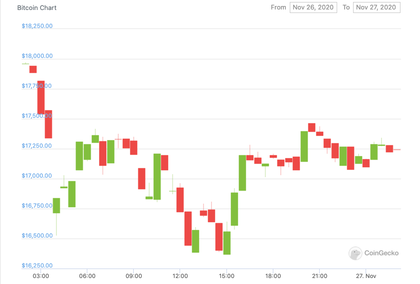\n",
314 | "\n",
315 | "Here is a description of the candle sticks.\n",
316 | "\n",
317 | " \n",
318 | "\n",
319 | "In this lab, we will be using the CoinGecko API to create one of these candlestick graphs for Bitcoin. We will use the API to get the price data for 30 days with 24 observation per day, 1 per hour. We will find the max, min, open, and close price per day meaning we will have 30 candlesticks and use that to generate the candlestick graph. Although we are using the CoinGecko API we will use a Python client/wrapper for the API called PyCoinGecko. PyCoinGecko will make performing the requests easy and it will deal with the enpoint targeting.\n"
320 | ]
321 | },
322 | {
323 | "cell_type": "markdown",
324 | "metadata": {},
325 | "source": [
326 | "Lets start off by getting the data we need. Using the \n",
318 | "\n",
319 | "In this lab, we will be using the CoinGecko API to create one of these candlestick graphs for Bitcoin. We will use the API to get the price data for 30 days with 24 observation per day, 1 per hour. We will find the max, min, open, and close price per day meaning we will have 30 candlesticks and use that to generate the candlestick graph. Although we are using the CoinGecko API we will use a Python client/wrapper for the API called PyCoinGecko. PyCoinGecko will make performing the requests easy and it will deal with the enpoint targeting.\n"
320 | ]
321 | },
322 | {
323 | "cell_type": "markdown",
324 | "metadata": {},
325 | "source": [
326 | "Lets start off by getting the data we need. Using the get_coin_market_chart_by_id(id, vs_currency, days). id is the name of the coin you want, vs_currency is the currency you want the price in, and days is how many days back from today you want.\n"
327 | ]
328 | },
329 | {
330 | "cell_type": "code",
331 | "execution_count": 10,
332 | "metadata": {},
333 | "outputs": [],
334 | "source": [
335 | "cg = CoinGeckoAPI()\n",
336 | "\n",
337 | "bitcoin_data = cg.get_coin_market_chart_by_id(id='bitcoin', vs_currency='usd', days=30)"
338 | ]
339 | },
340 | {
341 | "cell_type": "code",
342 | "execution_count": 11,
343 | "metadata": {},
344 | "outputs": [
345 | {
346 | "data": {
347 | "text/plain": [
348 | "dict"
349 | ]
350 | },
351 | "execution_count": 11,
352 | "metadata": {},
353 | "output_type": "execute_result"
354 | }
355 | ],
356 | "source": [
357 | "type(bitcoin_data )"
358 | ]
359 | },
360 | {
361 | "cell_type": "markdown",
362 | "metadata": {},
363 | "source": [
364 | "The response we get is in the form of a JSON which includes the price, market caps, and total volumes along with timestamps for each observation. We are focused on the prices so we will select that data.\n"
365 | ]
366 | },
367 | {
368 | "cell_type": "code",
369 | "execution_count": 12,
370 | "metadata": {},
371 | "outputs": [
372 | {
373 | "data": {
374 | "text/plain": [
375 | "[[1621836341055, 35363.48814978805],\n",
376 | " [1621841089336, 36251.58007239732],\n",
377 | " [1621843700749, 36778.04698988238],\n",
378 | " [1621847103260, 36651.72609163723],\n",
379 | " [1621850802945, 36339.00905215398]]"
380 | ]
381 | },
382 | "execution_count": 12,
383 | "metadata": {},
384 | "output_type": "execute_result"
385 | }
386 | ],
387 | "source": [
388 | "bitcoin_price_data = bitcoin_data['prices']\n",
389 | "\n",
390 | "bitcoin_price_data[0:5]"
391 | ]
392 | },
393 | {
394 | "cell_type": "markdown",
395 | "metadata": {},
396 | "source": [
397 | "Finally lets turn this data into a Pandas DataFrame.\n"
398 | ]
399 | },
400 | {
401 | "cell_type": "code",
402 | "execution_count": 13,
403 | "metadata": {},
404 | "outputs": [],
405 | "source": [
406 | "data = pd.DataFrame(bitcoin_price_data, columns=['TimeStamp', 'Price'])"
407 | ]
408 | },
409 | {
410 | "cell_type": "markdown",
411 | "metadata": {},
412 | "source": [
413 | "Now that we have the DataFrame we will convert the timestamp to datetime and save it as a column called Date. We will map our unix_to_datetime to each timestamp and convert it to a readable datetime.\n"
414 | ]
415 | },
416 | {
417 | "cell_type": "code",
418 | "execution_count": 14,
419 | "metadata": {},
420 | "outputs": [],
421 | "source": [
422 | "data['date'] = data['TimeStamp'].apply(lambda d: datetime.date.fromtimestamp(d/1000.0))\n"
423 | ]
424 | },
425 | {
426 | "cell_type": "markdown",
427 | "metadata": {},
428 | "source": [
429 | "Using this modified dataset we can now group by the Date and find the min, max, open, and close for the candlesticks.\n"
430 | ]
431 | },
432 | {
433 | "cell_type": "code",
434 | "execution_count": 15,
435 | "metadata": {},
436 | "outputs": [],
437 | "source": [
438 | "candlestick_data = data.groupby(data.date, as_index=False).agg({\"Price\": ['min', 'max', 'first', 'last']})"
439 | ]
440 | },
441 | {
442 | "cell_type": "markdown",
443 | "metadata": {},
444 | "source": [
445 | "Finally we are now ready to use plotly to create our Candlestick Chart.\n"
446 | ]
447 | },
448 | {
449 | "cell_type": "code",
450 | "execution_count": null,
451 | "metadata": {},
452 | "outputs": [],
453 | "source": [
454 | "fig = go.Figure(data=[go.Candlestick(x=candlestick_data['date'],\n",
455 | " open=candlestick_data['Price']['first'], \n",
456 | " high=candlestick_data['Price']['max'],\n",
457 | " low=candlestick_data['Price']['min'], \n",
458 | " close=candlestick_data['Price']['last'])\n",
459 | " ])\n",
460 | "\n",
461 | "fig.update_layout(xaxis_rangeslider_visible=False)\n",
462 | "\n",
463 | "fig.show()"
464 | ]
465 | },
466 | {
467 | "cell_type": "markdown",
468 | "metadata": {},
469 | "source": [
470 | "## Authors:\n",
471 | "\n",
472 | "## Change Log\n",
473 | "\n",
474 | "| Date (YYYY-MM-DD) | Version | Changed By | Change Description |\n",
475 | "|---|---|---|---|\n",
476 | "| 2020-11-23 | 3.0 | Azim Hirjani | New API |\n",
477 | "| 2020-09-09 | 2.1 | Malika Singla | Spell Check |\n",
478 | "| 2020-08-26 | 2.0 | Lavanya | Moved lab to course repo in GitLab |\n",
479 | "| | | | |\n",
480 | "\n",
481 | "
\n",
482 | "\n",
483 | "## © IBM Corporation 2020. All rights reserved. \n"
484 | ]
485 | },
486 | {
487 | "cell_type": "code",
488 | "execution_count": null,
489 | "metadata": {},
490 | "outputs": [],
491 | "source": []
492 | }
493 | ],
494 | "metadata": {
495 | "kernelspec": {
496 | "display_name": "Python",
497 | "language": "python",
498 | "name": "conda-env-python-py"
499 | },
500 | "language_info": {
501 | "codemirror_mode": {
502 | "name": "ipython",
503 | "version": 3
504 | },
505 | "file_extension": ".py",
506 | "mimetype": "text/x-python",
507 | "name": "python",
508 | "nbconvert_exporter": "python",
509 | "pygments_lexer": "ipython3",
510 | "version": "3.6.13"
511 | }
512 | },
513 | "nbformat": 4,
514 | "nbformat_minor": 4
515 | }
516 |
--------------------------------------------------------------------------------
/Python for Data Science, AI & Development/README.md:
--------------------------------------------------------------------------------
1 |
2 | [](https://github.com/ndleah?tab=repositories)
3 | [](https://github.com/ndleah)
4 |
5 | # Databases and SQL for Data Science
6 |
7 | ## About this Course
8 |
9 | This course will take you from zero to programming in Python in a matter of hours—no prior programming experience necessary! You will learn Python fundamentals, including data structures and data analysis, complete hands-on exercises throughout the course modules, and create a final project to demonstrate your new skills.
10 |
11 | By the end of this course, you’ll feel comfortable creating basic programs, working with data, and solving real-world problems in Python. You’ll gain a strong foundation for more advanced learning in the field, and develop skills to help advance your career.
12 |
13 | ## Modules
14 |
15 | * ### **Module 1 - Python Basics**
16 | This module teaches the basics of Python and begins by exploring some of the different data types such as integers, real numbers, and strings.
17 |
18 | * Your first program
19 | * Types
20 | * Expressions and Variables
21 | * String Operations
22 | * ### **Module 2 - Python Data Structures**
23 | This module begins a journey into Python data structures by explaining the use of lists and tuples and how they are able to store collections of data in a single variable.
24 |
25 | * Lists and Tuples
26 | * Sets
27 | * Dictionaries
28 | * ### **Module 3 - Python Programming Fundamentals**
29 | This module discusses Python fundamentals and begins with the concepts of conditions and branching.
30 |
31 | * Conditions and Branching
32 | * Loops
33 | * Functions
34 | * Objects and Classes
35 | * ### **Module 4 - Working with Data in Python**
36 | This module explains the basics of working with data in Python and begins the path with learning how to read and write files.
37 |
38 | * Reading files with open
39 | * Writing files with open
40 | * Loading data with Pandas
41 | * Numpy
42 | * ### **Module 5 - APIs, and Data Collection**
43 | This module delves into the unique ways to collect data by the use of APIs and webscraping.
44 |
45 | * Simple APIs
46 | * REST APIs & HTTP Requests
47 | * HTML for Webscraping
48 | * Webscraping
--------------------------------------------------------------------------------
/README.md:
--------------------------------------------------------------------------------
1 | 
2 | [](https://github.com/ndleah?tab=repositories)
3 | [](https://github.com/ndleah)
4 |
5 | # IBM Data Analyst Professional
6 |
7 | ## 📍 About this Professional Certificate
8 | Gain the **job-ready skills** for an entry-level data analyst role through this eight-course Professional Certificate from IBM and position yourself competitively in the thriving job market for data analysts, which will see a 20% growth until 2028 (U.S. Bureau of Labor Statistics).
9 |
10 | Power your data analyst career by learning the core principles of data analysis and gaining hands-on skills practice. You’ll work with a variety of data sources, project scenarios, and data analysis tools, including Excel, SQL, Python, Jupyter Notebooks, and Cognos Analytics, gaining practical experience with data manipulation and applying analytical techniques.
11 |
12 | ---
13 |
14 | ## 🥇 Professional Certificate
15 |
16 |
17 |  18 |
19 | ---
20 |
21 | ## 📙 Course Structures
22 |
23 | There are 9 Courses in this Professional Certificate Specialization are as follows:
24 |
25 | - [x] [__Introduction to Data Analytics__](https://github.com/ndleah/IBM-Data-Analyst-Professional/blob/main/certificate/Intro%20to%20Data%20Analysis-1.png)
26 |
27 | This course presents a gentle introduction into the concepts of data analysis, the role of a Data Analyst, and the tools that are used to perform daily functions. You will gain an understanding of the data ecosystem and the fundamentals of data analysis, such as data gathering or data mining.
28 |
29 |
18 |
19 | ---
20 |
21 | ## 📙 Course Structures
22 |
23 | There are 9 Courses in this Professional Certificate Specialization are as follows:
24 |
25 | - [x] [__Introduction to Data Analytics__](https://github.com/ndleah/IBM-Data-Analyst-Professional/blob/main/certificate/Intro%20to%20Data%20Analysis-1.png)
26 |
27 | This course presents a gentle introduction into the concepts of data analysis, the role of a Data Analyst, and the tools that are used to perform daily functions. You will gain an understanding of the data ecosystem and the fundamentals of data analysis, such as data gathering or data mining.
28 |
29 |
30 |  31 |
32 | - [x] [__Excel Basics for Data Analysis__](https://github.com/ndleah/IBM-Data-Analyst-Professional/tree/main/Excel%20Basics%20for%20Data%20Analysis)
33 |
34 | This course is designed to provide you with basic working knowledge for using Excel spreadsheets for Data Analysis. It covers some of the first steps for working with spreadsheets and their usage in the process of analyzing data. It includes plenty of videos, demos, and examples for you to learn, followed by step-by-step instructions for you to apply and practice on a live spreadsheet.
35 |
36 |
31 |
32 | - [x] [__Excel Basics for Data Analysis__](https://github.com/ndleah/IBM-Data-Analyst-Professional/tree/main/Excel%20Basics%20for%20Data%20Analysis)
33 |
34 | This course is designed to provide you with basic working knowledge for using Excel spreadsheets for Data Analysis. It covers some of the first steps for working with spreadsheets and their usage in the process of analyzing data. It includes plenty of videos, demos, and examples for you to learn, followed by step-by-step instructions for you to apply and practice on a live spreadsheet.
35 |
36 |
37 |  38 |
39 |
40 | - [X] [__Data Visualization and Dashboards with Excel and Cognos__ ](https://github.com/ndleah/IBM-Data-Analyst-Professional/tree/main/Data%20Visualization%20Dashboards%20Excel%20Cognos)
41 |
42 | This course covers some of the first steps in the development of data visualizations using spreadsheets and dashboards.
43 |
44 |
38 |
39 |
40 | - [X] [__Data Visualization and Dashboards with Excel and Cognos__ ](https://github.com/ndleah/IBM-Data-Analyst-Professional/tree/main/Data%20Visualization%20Dashboards%20Excel%20Cognos)
41 |
42 | This course covers some of the first steps in the development of data visualizations using spreadsheets and dashboards.
43 |
44 |
45 |  46 |
47 | - [x] [__Python for Data Science and AI__](https://github.com/ndleah/IBM-Data-Analyst-Professional/tree/main/Python%20for%20Data%20Science%2C%20AI%20%26%20Development)
48 |
49 | Kickstart your learning of Python for data science, as well as programming in general, with this beginner-friendly introduction to Python. Python is one of the world’s most popular programming languages, and there has never been greater demand for professionals with the ability to apply Python fundamentals to drive business solutions across industries.
50 |
51 |
46 |
47 | - [x] [__Python for Data Science and AI__](https://github.com/ndleah/IBM-Data-Analyst-Professional/tree/main/Python%20for%20Data%20Science%2C%20AI%20%26%20Development)
48 |
49 | Kickstart your learning of Python for data science, as well as programming in general, with this beginner-friendly introduction to Python. Python is one of the world’s most popular programming languages, and there has never been greater demand for professionals with the ability to apply Python fundamentals to drive business solutions across industries.
50 |
51 |
52 |  53 |
54 | - [X] [__Python Project for Data Science__](https://github.com/ndleah/IBM-Data-Analyst-Professional/tree/main/Python%20Project%20for%20Data%20Science)
55 |
56 | This mini-course is intended to for you to demonstrate foundational Python skills for working with data. The completion of this course involves working on a hands-on project where you will develop a simple dashboard using Python.
57 |
58 |
53 |
54 | - [X] [__Python Project for Data Science__](https://github.com/ndleah/IBM-Data-Analyst-Professional/tree/main/Python%20Project%20for%20Data%20Science)
55 |
56 | This mini-course is intended to for you to demonstrate foundational Python skills for working with data. The completion of this course involves working on a hands-on project where you will develop a simple dashboard using Python.
57 |
58 |
59 |  60 |
61 | - [x] [__Databases and SQL for Data Science__](https://github.com/ndleah/IBM-Data-Analyst-Professional/tree/main/Databases%20and%20SQL%20for%20Data%20Science%20with%20Python)
62 |
63 | The purpose of this course is to introduce relational database concepts and help you learn and apply foundational knowledge of the SQL language. It is also intended to get you started with performing SQL access in a data science environment.
64 |
65 |
60 |
61 | - [x] [__Databases and SQL for Data Science__](https://github.com/ndleah/IBM-Data-Analyst-Professional/tree/main/Databases%20and%20SQL%20for%20Data%20Science%20with%20Python)
62 |
63 | The purpose of this course is to introduce relational database concepts and help you learn and apply foundational knowledge of the SQL language. It is also intended to get you started with performing SQL access in a data science environment.
64 |
65 |
66 |  67 |
68 | - [x] [__Data Analysis with Python__](https://github.com/ndleah/IBM-Data-Analyst-Professional/tree/main/Data%20Analysis%20With%20Python)
69 |
70 | Learn how to analyze data using Python. Topics covered:
71 |
72 | 1) Importing Datasets
73 | 2) Cleaning the Data
74 | 3) Data frame manipulation
75 | 4) Summarizing the Data
76 | 5) Building machine learning Regression models
77 | 6) Building data pipelines
78 |
79 |
67 |
68 | - [x] [__Data Analysis with Python__](https://github.com/ndleah/IBM-Data-Analyst-Professional/tree/main/Data%20Analysis%20With%20Python)
69 |
70 | Learn how to analyze data using Python. Topics covered:
71 |
72 | 1) Importing Datasets
73 | 2) Cleaning the Data
74 | 3) Data frame manipulation
75 | 4) Summarizing the Data
76 | 5) Building machine learning Regression models
77 | 6) Building data pipelines
78 |
79 |
80 |  81 |
82 | - [x] [__Data Visualization with Python__](https://github.com/ndleah/IBM-Data-Analyst-Professional/tree/main/Data%20Visualization%20with%20Python)
83 |
84 | The main goal of this Data Visualization with Python course is to teach you how to take data that at first glance has little meaning and present that data in a form that makes sense to people. Various techniques have been developed for presenting data visually but in this course, we will be using several data visualization libraries in Python, namely Matplotlib, Seaborn, and Folium.
85 |
86 |
81 |
82 | - [x] [__Data Visualization with Python__](https://github.com/ndleah/IBM-Data-Analyst-Professional/tree/main/Data%20Visualization%20with%20Python)
83 |
84 | The main goal of this Data Visualization with Python course is to teach you how to take data that at first glance has little meaning and present that data in a form that makes sense to people. Various techniques have been developed for presenting data visually but in this course, we will be using several data visualization libraries in Python, namely Matplotlib, Seaborn, and Folium.
85 |
86 |
87 |  88 |
89 | - [x] [__IBM Data Analyst Capstone Project__](https://github.com/ndleah/IBM-Data-Analyst-Professional/tree/main/Data%20Analyst%20Capstone%20Project)
90 |
91 | In this course you will apply various Data Analytics skills and techniques that you have learned as part of the previous courses in the IBM Data Analyst Professional Certificate. You will assume the role of an Associate Data Analyst who has recently joined the organization and be presented with a business challenge that requires data analysis to be performed on real-world datasets.
92 |
93 |
88 |
89 | - [x] [__IBM Data Analyst Capstone Project__](https://github.com/ndleah/IBM-Data-Analyst-Professional/tree/main/Data%20Analyst%20Capstone%20Project)
90 |
91 | In this course you will apply various Data Analytics skills and techniques that you have learned as part of the previous courses in the IBM Data Analyst Professional Certificate. You will assume the role of an Associate Data Analyst who has recently joined the organization and be presented with a business challenge that requires data analysis to be performed on real-world datasets.
92 |
93 |
94 |  95 |
96 | ---
97 |
95 |
96 | ---
97 | © 2021 Leah Nguyen
98 |
--------------------------------------------------------------------------------
/certificate/8H6UT8SHWYPD-1.png:
--------------------------------------------------------------------------------
https://raw.githubusercontent.com/ndleah/IBM-data-analyst-professional/708fa3e19d49d501f888be623d77170719c8d046/certificate/8H6UT8SHWYPD-1.png
--------------------------------------------------------------------------------
/certificate/Data Analysis with Python-1.png:
--------------------------------------------------------------------------------
https://raw.githubusercontent.com/ndleah/IBM-data-analyst-professional/708fa3e19d49d501f888be623d77170719c8d046/certificate/Data Analysis with Python-1.png
--------------------------------------------------------------------------------
/certificate/Data Visualization and Dashboards with Excel and Cognos-1.png:
--------------------------------------------------------------------------------
https://raw.githubusercontent.com/ndleah/IBM-data-analyst-professional/708fa3e19d49d501f888be623d77170719c8d046/certificate/Data Visualization and Dashboards with Excel and Cognos-1.png
--------------------------------------------------------------------------------
/certificate/Data Visualization with Python-1.png:
--------------------------------------------------------------------------------
https://raw.githubusercontent.com/ndleah/IBM-data-analyst-professional/708fa3e19d49d501f888be623d77170719c8d046/certificate/Data Visualization with Python-1.png
--------------------------------------------------------------------------------
/certificate/Database SQL Data Science-1.png:
--------------------------------------------------------------------------------
https://raw.githubusercontent.com/ndleah/IBM-data-analyst-professional/708fa3e19d49d501f888be623d77170719c8d046/certificate/Database SQL Data Science-1.png
--------------------------------------------------------------------------------
/certificate/Excel Basic for Data Analysis-1.png:
--------------------------------------------------------------------------------
https://raw.githubusercontent.com/ndleah/IBM-data-analyst-professional/708fa3e19d49d501f888be623d77170719c8d046/certificate/Excel Basic for Data Analysis-1.png
--------------------------------------------------------------------------------
/certificate/IBM Data Analyst Capstone Project-1.png:
--------------------------------------------------------------------------------
https://raw.githubusercontent.com/ndleah/IBM-data-analyst-professional/708fa3e19d49d501f888be623d77170719c8d046/certificate/IBM Data Analyst Capstone Project-1.png
--------------------------------------------------------------------------------
/certificate/Intro to Data Analysis-1.png:
--------------------------------------------------------------------------------
https://raw.githubusercontent.com/ndleah/IBM-data-analyst-professional/708fa3e19d49d501f888be623d77170719c8d046/certificate/Intro to Data Analysis-1.png
--------------------------------------------------------------------------------
/certificate/Python Project for Data Science AI-1.png:
--------------------------------------------------------------------------------
https://raw.githubusercontent.com/ndleah/IBM-data-analyst-professional/708fa3e19d49d501f888be623d77170719c8d046/certificate/Python Project for Data Science AI-1.png
--------------------------------------------------------------------------------
/certificate/Python for AI, Data Science Development-1.png:
--------------------------------------------------------------------------------
https://raw.githubusercontent.com/ndleah/IBM-data-analyst-professional/708fa3e19d49d501f888be623d77170719c8d046/certificate/Python for AI, Data Science Development-1.png
--------------------------------------------------------------------------------
|
 36 |
36 |  40 |
40 |  44 |
44 |  48 |
48 |  52 |
52 |  56 |
56 |  60 |
60 |  64 |
64 |  68 |
68 |  \n",
9 | "
\n",
9 | " \n",
38 | " \n",
39 | "
\n",
38 | " \n",
39 | "