├── .github
├── .gitignore
└── workflows
│ ├── pkgdown.yaml
│ ├── R-CMD-check.yaml
│ └── docker-build.yml
├── data-raw
├── .gitignore
├── test-omitted-ways.qmd
├── traffic_volumes_edinburgh.R
├── test-sett.qmd
├── osm_edinburgh.R
├── calculateAverageWidths.R
├── tests.Rmd
└── gisruk2025.qmd
├── vignettes
├── .gitignore
├── images
│ └── paste-1.png
├── classifying-cycle-infrastructure.qmd
├── references.bib
├── classify-cbd.Rmd
└── gisruk2025.Rmd
├── LICENSE
├── street_space.png
├── data
├── cycle_net_f.rda
├── drive_net_f.rda
├── osm_edinburgh.rda
├── los_table_complete.rda
├── traffic_random_edinburgh.rda
└── traffic_volumes_edinburgh.rda
├── _pkgdown.yml
├── edinburgh_bus_lanes.png
├── man
├── figures
│ ├── README-leeds-1.png
│ ├── README-bristol-1.png
│ ├── README-dublin-1.png
│ ├── README-lisbon-1.png
│ ├── README-london-1.png
│ ├── README-cambridge-1.png
│ ├── README-edinburgh-1.png
│ ├── README-christchurch-1.png
│ ├── README-christchurch-2.png
│ ├── README-unnamed-chunk-8-1.png
│ ├── README-level_of_service-1.png
│ └── README-minimal_plot_osm-1.png
├── et_active.Rd
├── cycle_net_f.Rd
├── drive_net_f.Rd
├── osm_edinburgh.Rd
├── count_bus_lanes.Rd
├── traffic_volumes_edinburgh.Rd
├── get_active_travel_network.Rd
├── npt_to_cbd_aadt.Rd
├── get_palette_npt.Rd
├── classify_speeds.Rd
├── get_cycling_network.Rd
├── npt_to_cbd_aadt_numeric.Rd
├── get_points.Rd
├── clean_widths.Rd
├── los_table_complete.Rd
├── get_traffic_calming.Rd
├── is_wide.Rd
├── estimate_traffic.Rd
├── clean_speeds.Rd
├── get_driving_network.Rd
├── plot_osm_tmap.Rd
├── npt_to_cbd_aadt_character.Rd
├── distance_to_road.Rd
├── get_bus_routes.Rd
├── classify_shared_use.Rd
├── get_travel_network.Rd
├── level_of_service.Rd
├── classify_cycle_infrastructure.Rd
└── get_parallel_values.Rd
├── .devcontainer
└── devcontainer.json
├── R
├── globals.R
├── test-code
│ └── portugal.R
└── get_parallel_values.R
├── .Rbuildignore
├── Dockerfile
├── app
├── Dockerfile
└── app.R
├── .gitignore
├── LICENSE.md
├── DESCRIPTION
├── NAMESPACE
├── inst
└── extdata
│ ├── level-of-service-table.csv
│ └── los_table_complete.csv
├── code
├── traffic-volumes.R
└── classify-roads.R
└── README.Rmd
/.github/.gitignore:
--------------------------------------------------------------------------------
1 | *.html
2 |
--------------------------------------------------------------------------------
/data-raw/.gitignore:
--------------------------------------------------------------------------------
1 | /.quarto/
2 |
--------------------------------------------------------------------------------
/vignettes/.gitignore:
--------------------------------------------------------------------------------
1 | *.html
2 | *.R
3 |
4 | /.quarto/
5 |
--------------------------------------------------------------------------------
/LICENSE:
--------------------------------------------------------------------------------
1 | YEAR: 2024
2 | COPYRIGHT HOLDER: Robin Lovelace
3 |
--------------------------------------------------------------------------------
/street_space.png:
--------------------------------------------------------------------------------
https://raw.githubusercontent.com/nptscot/osmactive/HEAD/street_space.png
--------------------------------------------------------------------------------
/data/cycle_net_f.rda:
--------------------------------------------------------------------------------
https://raw.githubusercontent.com/nptscot/osmactive/HEAD/data/cycle_net_f.rda
--------------------------------------------------------------------------------
/data/drive_net_f.rda:
--------------------------------------------------------------------------------
https://raw.githubusercontent.com/nptscot/osmactive/HEAD/data/drive_net_f.rda
--------------------------------------------------------------------------------
/_pkgdown.yml:
--------------------------------------------------------------------------------
1 | url: https://nptscot.github.io/osmactive/
2 | template:
3 | bootstrap: 5
4 |
5 |
--------------------------------------------------------------------------------
/data/osm_edinburgh.rda:
--------------------------------------------------------------------------------
https://raw.githubusercontent.com/nptscot/osmactive/HEAD/data/osm_edinburgh.rda
--------------------------------------------------------------------------------
/edinburgh_bus_lanes.png:
--------------------------------------------------------------------------------
https://raw.githubusercontent.com/nptscot/osmactive/HEAD/edinburgh_bus_lanes.png
--------------------------------------------------------------------------------
/data/los_table_complete.rda:
--------------------------------------------------------------------------------
https://raw.githubusercontent.com/nptscot/osmactive/HEAD/data/los_table_complete.rda
--------------------------------------------------------------------------------
/man/figures/README-leeds-1.png:
--------------------------------------------------------------------------------
https://raw.githubusercontent.com/nptscot/osmactive/HEAD/man/figures/README-leeds-1.png
--------------------------------------------------------------------------------
/vignettes/images/paste-1.png:
--------------------------------------------------------------------------------
https://raw.githubusercontent.com/nptscot/osmactive/HEAD/vignettes/images/paste-1.png
--------------------------------------------------------------------------------
/man/figures/README-bristol-1.png:
--------------------------------------------------------------------------------
https://raw.githubusercontent.com/nptscot/osmactive/HEAD/man/figures/README-bristol-1.png
--------------------------------------------------------------------------------
/man/figures/README-dublin-1.png:
--------------------------------------------------------------------------------
https://raw.githubusercontent.com/nptscot/osmactive/HEAD/man/figures/README-dublin-1.png
--------------------------------------------------------------------------------
/man/figures/README-lisbon-1.png:
--------------------------------------------------------------------------------
https://raw.githubusercontent.com/nptscot/osmactive/HEAD/man/figures/README-lisbon-1.png
--------------------------------------------------------------------------------
/man/figures/README-london-1.png:
--------------------------------------------------------------------------------
https://raw.githubusercontent.com/nptscot/osmactive/HEAD/man/figures/README-london-1.png
--------------------------------------------------------------------------------
/data/traffic_random_edinburgh.rda:
--------------------------------------------------------------------------------
https://raw.githubusercontent.com/nptscot/osmactive/HEAD/data/traffic_random_edinburgh.rda
--------------------------------------------------------------------------------
/data/traffic_volumes_edinburgh.rda:
--------------------------------------------------------------------------------
https://raw.githubusercontent.com/nptscot/osmactive/HEAD/data/traffic_volumes_edinburgh.rda
--------------------------------------------------------------------------------
/man/figures/README-cambridge-1.png:
--------------------------------------------------------------------------------
https://raw.githubusercontent.com/nptscot/osmactive/HEAD/man/figures/README-cambridge-1.png
--------------------------------------------------------------------------------
/man/figures/README-edinburgh-1.png:
--------------------------------------------------------------------------------
https://raw.githubusercontent.com/nptscot/osmactive/HEAD/man/figures/README-edinburgh-1.png
--------------------------------------------------------------------------------
/man/figures/README-christchurch-1.png:
--------------------------------------------------------------------------------
https://raw.githubusercontent.com/nptscot/osmactive/HEAD/man/figures/README-christchurch-1.png
--------------------------------------------------------------------------------
/man/figures/README-christchurch-2.png:
--------------------------------------------------------------------------------
https://raw.githubusercontent.com/nptscot/osmactive/HEAD/man/figures/README-christchurch-2.png
--------------------------------------------------------------------------------
/man/figures/README-unnamed-chunk-8-1.png:
--------------------------------------------------------------------------------
https://raw.githubusercontent.com/nptscot/osmactive/HEAD/man/figures/README-unnamed-chunk-8-1.png
--------------------------------------------------------------------------------
/man/figures/README-level_of_service-1.png:
--------------------------------------------------------------------------------
https://raw.githubusercontent.com/nptscot/osmactive/HEAD/man/figures/README-level_of_service-1.png
--------------------------------------------------------------------------------
/man/figures/README-minimal_plot_osm-1.png:
--------------------------------------------------------------------------------
https://raw.githubusercontent.com/nptscot/osmactive/HEAD/man/figures/README-minimal_plot_osm-1.png
--------------------------------------------------------------------------------
/.devcontainer/devcontainer.json:
--------------------------------------------------------------------------------
1 | {
2 | "name": "osmactive Dev Container",
3 | "image": "ghcr.io/nptscot/osmactive",
4 | "extensions": [
5 | "quarto.quarto",
6 | "reditorsupport.r"
7 | ],
8 | "remoteUser": "rstudio"
9 | }
10 |
11 |
--------------------------------------------------------------------------------
/R/globals.R:
--------------------------------------------------------------------------------
1 | utils::globalVariables(c(
2 | "cycle_pedestrian_separation", "bicycle", "surface", "smoothness",
3 | "cycleway_left", "oneway", "cycleway_right", "osm_id",
4 | "azimuth_target", "azimuth_source", "new_values", "angle_diff",
5 | ":=", "new_value", "new_value_numeric", "service",
6 | "los_table_complete", "los"
7 | ))
--------------------------------------------------------------------------------
/.Rbuildignore:
--------------------------------------------------------------------------------
1 | ^README\.Rmd$
2 | ^LICENSE\.md$
3 | ^_pkgdown\.yml$
4 | ^docs$
5 | ^pkgdown$
6 | ^\.github$
7 | ^data-raw$
8 | ^.*\.Rproj$
9 | ^\.Rproj\.user$
10 | cache
11 | .*\.Rds$
12 | ^\.devcontainer$
13 | ^app$
14 | ^code$
15 | ^edinburgh_bus_lanes\.png$
16 | ^street_space\.png$
17 | ^cycle_net\.geojson$
18 | ^osm_district\.geojson$
19 |
--------------------------------------------------------------------------------
/man/et_active.Rd:
--------------------------------------------------------------------------------
1 | % Generated by roxygen2: do not edit by hand
2 | % Please edit documentation in R/osmactive.R
3 | \name{et_active}
4 | \alias{et_active}
5 | \title{This function returns OSM keys that are relevant for active travel}
6 | \usage{
7 | et_active()
8 | }
9 | \description{
10 | This function returns OSM keys that are relevant for active travel
11 | }
12 |
--------------------------------------------------------------------------------
/Dockerfile:
--------------------------------------------------------------------------------
1 | FROM ghcr.io/geocompx/latest@sha256:00ff6dd552f2e9168488dee6ee1babb4b6bee805f0a2d35aff548d6ee2730625
2 |
3 | # Set the working directory
4 | WORKDIR /app
5 |
6 | # Copy the current directory contents into the container
7 | COPY . /app
8 |
9 | # Install the osmactive package
10 | RUN R -e 'remotes::install_local(dependencies = TRUE)' && \
11 | R -e 'library(osmactive)'
12 |
--------------------------------------------------------------------------------
/man/cycle_net_f.Rd:
--------------------------------------------------------------------------------
1 | % Generated by roxygen2: do not edit by hand
2 | % Please edit documentation in R/osmactive.R
3 | \name{cycle_net_f}
4 | \alias{cycle_net_f}
5 | \title{Cycle network for Edinburgh, filtered around Leith Walk}
6 | \format{
7 | An sf data frame
8 | }
9 | \description{
10 | This dataset contains the cycle network for Edinburgh, filtered around Leith Walk.
11 | }
12 | \examples{
13 | head(cycle_net_f)
14 | plot(cycle_net_f)
15 | }
16 |
--------------------------------------------------------------------------------
/man/drive_net_f.Rd:
--------------------------------------------------------------------------------
1 | % Generated by roxygen2: do not edit by hand
2 | % Please edit documentation in R/osmactive.R
3 | \name{drive_net_f}
4 | \alias{drive_net_f}
5 | \title{Driving network for Edinburgh, filtered around Leith Walk}
6 | \format{
7 | An sf data frame
8 | }
9 | \description{
10 | This dataset contains the driving network for Edinburgh, filtered around Leith Walk.
11 | }
12 | \examples{
13 | head(drive_net_f)
14 | plot(drive_net_f)
15 | }
16 |
--------------------------------------------------------------------------------
/man/osm_edinburgh.Rd:
--------------------------------------------------------------------------------
1 | % Generated by roxygen2: do not edit by hand
2 | % Please edit documentation in R/osmactive.R
3 | \docType{data}
4 | \name{osm_edinburgh}
5 | \alias{osm_edinburgh}
6 | \title{Data from edinburgh's OSM network}
7 | \format{
8 | An sf data frame
9 | }
10 | \description{
11 | Data from edinburgh's OSM network
12 | }
13 | \examples{
14 | library(sf)
15 | names(osm_edinburgh)
16 | head(osm_edinburgh)
17 | plot(osm_edinburgh)
18 | }
19 | \keyword{datasets}
20 |
--------------------------------------------------------------------------------
/man/count_bus_lanes.Rd:
--------------------------------------------------------------------------------
1 | % Generated by roxygen2: do not edit by hand
2 | % Please edit documentation in R/osmactive.R
3 | \name{count_bus_lanes}
4 | \alias{count_bus_lanes}
5 | \title{Count how many bus lanes there are}
6 | \usage{
7 | count_bus_lanes(osm)
8 | }
9 | \arguments{
10 | \item{osm}{An sf object with the road network}
11 | }
12 | \value{
13 | The number of bus lanes
14 | }
15 | \description{
16 | Count how many bus lanes there are
17 | }
18 | \examples{
19 | osm = osm_edinburgh
20 | count_bus_lanes(osm)
21 | }
22 |
--------------------------------------------------------------------------------
/man/traffic_volumes_edinburgh.Rd:
--------------------------------------------------------------------------------
1 | % Generated by roxygen2: do not edit by hand
2 | % Please edit documentation in R/osmactive.R
3 | \docType{data}
4 | \name{traffic_volumes_edinburgh}
5 | \alias{traffic_volumes_edinburgh}
6 | \alias{traffic_random_edinburgh}
7 | \title{Data from edinburgh's OSM network with traffic volumes}
8 | \format{
9 | A data frame
10 | }
11 | \description{
12 | Data from edinburgh's OSM network with traffic volumes
13 | }
14 | \examples{
15 | head(traffic_volumes_edinburgh)
16 | head(traffic_random_edinburgh)
17 | }
18 | \keyword{datasets}
19 |
--------------------------------------------------------------------------------
/data-raw/test-omitted-ways.qmd:
--------------------------------------------------------------------------------
1 | The aim of the code below is to test which ways are omitted by the `get_cycling_network` function.
2 |
3 |
4 | ```{r}
5 | devtools::load_all()
6 | library(tidyverse)
7 | osm_national = get_travel_network("Scotland")
8 | osm_trinity_crescent = osm_national |>
9 | filter(name == "Trinity Crescent")
10 | mapview::mapview(osm_trinity_crescent)
11 |
12 | # Use browser() for interactive debugging in the following line:
13 | devtools::load_all()
14 | osm_trinity_filtered = get_cycling_network(osm_trinity_crescent)
15 | mapview::mapview(osm_trinity_filtered)
16 | ```
--------------------------------------------------------------------------------
/man/get_active_travel_network.Rd:
--------------------------------------------------------------------------------
1 | % Generated by roxygen2: do not edit by hand
2 | % Please edit documentation in R/osmactive.R
3 | \name{get_active_travel_network}
4 | \alias{get_active_travel_network}
5 | \title{Get the OSM cycling network}
6 | \usage{
7 | get_active_travel_network(osm)
8 | }
9 | \arguments{
10 | \item{osm}{An OSM network object}
11 | }
12 | \value{
13 | A sf object with the OSM network relevant for active travel
14 | with columns containing information on traffic calming measures,
15 | crossings, cycle infrastructure, and more.
16 | }
17 | \description{
18 | Get the OSM cycling network
19 | }
20 |
--------------------------------------------------------------------------------
/man/npt_to_cbd_aadt.Rd:
--------------------------------------------------------------------------------
1 | % Generated by roxygen2: do not edit by hand
2 | % Please edit documentation in R/osmactive.R
3 | \name{npt_to_cbd_aadt}
4 | \alias{npt_to_cbd_aadt}
5 | \title{Convert AADT to CBD AADT}
6 | \usage{
7 | npt_to_cbd_aadt(AADT)
8 | }
9 | \arguments{
10 | \item{AADT}{A character or numeric value representing the Annual Average Daily Traffic.}
11 | }
12 | \value{
13 | The converted CBD AADT value.
14 | }
15 | \description{
16 | This function converts Annual Average Daily Traffic (AADT) to Central Business District (CBD) AADT.
17 | It handles both character and numeric inputs by delegating to appropriate helper functions.
18 | }
19 |
--------------------------------------------------------------------------------
/man/get_palette_npt.Rd:
--------------------------------------------------------------------------------
1 | % Generated by roxygen2: do not edit by hand
2 | % Please edit documentation in R/osmactive.R
3 | \name{get_palette_npt}
4 | \alias{get_palette_npt}
5 | \title{Get the palette for the NPT cycle segregation levels}
6 | \usage{
7 | get_palette_npt()
8 | }
9 | \value{
10 | A palette for the NPT cycle segregation levels
11 | }
12 | \description{
13 | Get the palette for the NPT cycle segregation levels
14 | }
15 | \examples{
16 | cols = get_palette_npt()
17 | jsonlite::toJSON(as.list(cols), pretty = TRUE)
18 | col_labs = c("OffRd", "SegW", "SegN", "Share", "Paint")
19 | barplot(seq_along(cols), col = cols, names.arg = col_labs)
20 | }
21 |
--------------------------------------------------------------------------------
/man/classify_speeds.Rd:
--------------------------------------------------------------------------------
1 | % Generated by roxygen2: do not edit by hand
2 | % Please edit documentation in R/osmactive.R
3 | \name{classify_speeds}
4 | \alias{classify_speeds}
5 | \title{Classify Speeds}
6 | \usage{
7 | classify_speeds(speed_mph)
8 | }
9 | \arguments{
10 | \item{speed_mph}{A numeric vector representing speeds in miles per hour.}
11 | }
12 | \value{
13 | A character vector with the speed categories.
14 | }
15 | \description{
16 | This function classifies speeds in miles per hour (mph) into categories.
17 | }
18 | \examples{
19 | classify_speeds(c(15, 25, 35, 45, 55, 65))
20 | # Returns: "<20 mph", "20 mph", "30 mph", "40 mph", "50 mph", "60+ mph"
21 | }
22 |
--------------------------------------------------------------------------------
/man/get_cycling_network.Rd:
--------------------------------------------------------------------------------
1 | % Generated by roxygen2: do not edit by hand
2 | % Please edit documentation in R/osmactive.R
3 | \name{get_cycling_network}
4 | \alias{get_cycling_network}
5 | \title{Get the OSM cycling network}
6 | \usage{
7 | get_cycling_network(
8 | osm,
9 | ex_c = exclude_highway_cycling(),
10 | ex_b = exclude_bicycle_cycling()
11 | )
12 | }
13 | \arguments{
14 | \item{osm}{An OSM network object}
15 |
16 | \item{ex_c}{A vector of highway values to exclude}
17 |
18 | \item{ex_b}{A vector of bicycle values to exclude}
19 | }
20 | \value{
21 | A sf object with the OSM cycling network
22 | }
23 | \description{
24 | Get the OSM cycling network
25 | }
26 |
--------------------------------------------------------------------------------
/man/npt_to_cbd_aadt_numeric.Rd:
--------------------------------------------------------------------------------
1 | % Generated by roxygen2: do not edit by hand
2 | % Please edit documentation in R/osmactive.R
3 | \name{npt_to_cbd_aadt_numeric}
4 | \alias{npt_to_cbd_aadt_numeric}
5 | \title{Convert AADT categories to CBD AADT character ranges}
6 | \usage{
7 | npt_to_cbd_aadt_numeric(AADT)
8 | }
9 | \arguments{
10 | \item{AADT}{A numeric vector representing AADT}
11 | }
12 | \value{
13 | A character vector with the converted CBD AADT ranges. Possible return values are "0 to 999", "1000 to 1999", "2000 to 3999", and "4000+".
14 | }
15 | \description{
16 | This function takes an AADT (Annual Average Daily Traffic) category and converts it to a ranges
17 | }
18 |
--------------------------------------------------------------------------------
/man/get_points.Rd:
--------------------------------------------------------------------------------
1 | % Generated by roxygen2: do not edit by hand
2 | % Please edit documentation in R/osmactive.R
3 | \name{get_points}
4 | \alias{get_points}
5 | \title{Get the OSM network functions}
6 | \usage{
7 | get_points(place, extra_tags = c("traffic_calming", "crossing"), ...)
8 | }
9 | \arguments{
10 | \item{place}{A place name or a bounding box passed to \code{osmextract::oe_get()}}
11 |
12 | \item{extra_tags}{A vector of extra tags to be included in the OSM extract}
13 |
14 | \item{...}{Additional arguments passed to \code{osmextract::oe_get()}}
15 | }
16 | \value{
17 | A sf object with the OSM network
18 | }
19 | \description{
20 | Get the OSM network functions
21 | }
22 |
--------------------------------------------------------------------------------
/man/clean_widths.Rd:
--------------------------------------------------------------------------------
1 | % Generated by roxygen2: do not edit by hand
2 | % Please edit documentation in R/osmactive.R
3 | \name{clean_widths}
4 | \alias{clean_widths}
5 | \title{Clean cycleway widths (use est_widths when available and width otherwise)}
6 | \usage{
7 | clean_widths(osm)
8 | }
9 | \arguments{
10 | \item{osm}{An sf object with the road network}
11 | }
12 | \value{
13 | An sf object with the cleaned cycleway widths in the column \code{width}
14 | }
15 | \description{
16 | Clean cycleway widths (use est_widths when available and width otherwise)
17 | }
18 | \examples{
19 | osm = osm_edinburgh
20 | osm$width
21 | osm$est_width = NA
22 | osm$est_width[1:3] = 2
23 | osm_cleaned = clean_widths(osm)
24 | osm$width
25 | osm_cleaned$width
26 | }
27 |
--------------------------------------------------------------------------------
/man/los_table_complete.Rd:
--------------------------------------------------------------------------------
1 | % Generated by roxygen2: do not edit by hand
2 | % Please edit documentation in R/osmactive.R
3 | \name{los_table_complete}
4 | \alias{los_table_complete}
5 | \title{Complete Level of Service (LOS) table}
6 | \format{
7 | A data frame with columns including speed limit, AADT, cycle_segregation and level_of_service
8 | }
9 | \source{
10 | Generated from the classify-cbd vignette
11 | }
12 | \usage{
13 | data(los_table_complete)
14 | }
15 | \description{
16 | This dataset contains the complete level of service information, including missing categories, in a long format.
17 | }
18 | \examples{
19 | data(los_table_complete)
20 | cols = c("Speed Limit (mph)", "Speed (85th kph)")
21 | unique(los_table_complete[cols])
22 | head(los_table_complete)
23 | }
24 |
--------------------------------------------------------------------------------
/app/Dockerfile:
--------------------------------------------------------------------------------
1 | FROM rocker/geospatial:latest
2 |
3 | RUN /rocker_scripts/setup_R.sh https://packagemanager.posit.co/cran/__linux__/jammy/2023-01-29
4 | RUN /rocker_scripts/install_shiny_server.sh
5 |
6 | # Install any necessary R packages
7 | RUN R -e "install.packages(c('remotes'))"
8 | RUN R -e "install.packages(c('cols4all', 'geos', 'osmextract'))"
9 | RUN R -e "install.packages(c('shiny', 'tmap'))"
10 | RUN R -e "remotes::install_github('nptscot/osmactive', dependencies = 'Suggests', ask = FALSE, Ncpus = parallel::detectCores())"
11 |
12 |
13 | # Copy the application files into the container
14 | COPY app.R /app/app.R
15 |
16 | # Expose port 3838
17 | EXPOSE 3838
18 |
19 | # Start the Shiny app
20 | CMD ["R", "-e", "shiny::runApp('/app/app.R', host = '0.0.0.0', port = 3838)"]
--------------------------------------------------------------------------------
/man/get_traffic_calming.Rd:
--------------------------------------------------------------------------------
1 | % Generated by roxygen2: do not edit by hand
2 | % Please edit documentation in R/osmactive.R
3 | \name{get_traffic_calming}
4 | \alias{get_traffic_calming}
5 | \title{Get the OSM network functions}
6 | \usage{
7 | get_traffic_calming(osm_points, filter = TRUE)
8 | }
9 | \arguments{
10 | \item{osm_points}{An sf object with the OSM network}
11 |
12 | \item{filter}{Whether to filter the results to only include traffic calming measures}
13 | }
14 | \value{
15 | A data frame with the OSM network relevant for active travel
16 | }
17 | \description{
18 | Get the OSM network functions
19 | }
20 | \examples{
21 | osm_points = get_points("Edinburgh")
22 | traffic_calming = get_traffic_calming(osm_points)
23 | head(traffic_calming)
24 | plot(traffic_calming["traffic_calming"])
25 | }
26 |
--------------------------------------------------------------------------------
/man/is_wide.Rd:
--------------------------------------------------------------------------------
1 | % Generated by roxygen2: do not edit by hand
2 | % Please edit documentation in R/osmactive.R
3 | \name{is_wide}
4 | \alias{is_wide}
5 | \title{Classify Separated cycle track by width}
6 | \usage{
7 | is_wide(x, min_width = 2)
8 | }
9 | \arguments{
10 | \item{x}{A numeric vector with the width of the cycleway (m)}
11 |
12 | \item{min_width}{The minimum width for a cycleway to be considered wide (m)}
13 | }
14 | \value{
15 | A logical vector indicating whether the cycleway is wide
16 | }
17 | \description{
18 | This function classifies cycleways as wide if the width is greater than or equal to \code{min_width}.
19 | NA values are replaced with 0, meaning that ways with no measurement are considered narrow.
20 | }
21 | \examples{
22 | x = osm_edinburgh$width
23 | x
24 | is_wide(x)
25 | }
26 |
--------------------------------------------------------------------------------
/man/estimate_traffic.Rd:
--------------------------------------------------------------------------------
1 | % Generated by roxygen2: do not edit by hand
2 | % Please edit documentation in R/osmactive.R
3 | \name{estimate_traffic}
4 | \alias{estimate_traffic}
5 | \title{Estimate traffic}
6 | \usage{
7 | estimate_traffic(osm)
8 | }
9 | \arguments{
10 | \item{osm}{An sf object with the road network}
11 | }
12 | \value{
13 | An sf object with the estimated road traffic volumes in the column \code{assumed_volume}
14 | }
15 | \description{
16 | Estimate traffic
17 | }
18 | \examples{
19 | osm = osm_edinburgh
20 | osm_traffic = estimate_traffic(osm)
21 | # check NAs:
22 | sel_nas = is.na(osm_traffic$assumed_volume)
23 | osm_no_traffic = osm_traffic[sel_nas, c("highway")]
24 | table(osm_no_traffic$highway) # Active travel infrastructure has no road traffic
25 | table(osm_traffic$assumed_volume, useNA = "always")
26 | }
27 |
--------------------------------------------------------------------------------
/man/clean_speeds.Rd:
--------------------------------------------------------------------------------
1 | % Generated by roxygen2: do not edit by hand
2 | % Please edit documentation in R/osmactive.R
3 | \name{clean_speeds}
4 | \alias{clean_speeds}
5 | \title{Clean speeds}
6 | \usage{
7 | clean_speeds(osm)
8 | }
9 | \arguments{
10 | \item{osm}{An sf object with the road network}
11 | }
12 | \value{
13 | An sf object with the cleaned speed values in the column \code{maxspeed_clean}
14 | }
15 | \description{
16 | Clean speeds
17 | }
18 | \examples{
19 | osm = osm_edinburgh
20 | osm_cleaned = clean_speeds(osm)
21 | # check NAs:
22 | sel_nas = is.na(osm_cleaned$maxspeed_clean)
23 | osm_no_maxspeed = osm_cleaned[sel_nas, c("highway")]
24 | table(osm_no_maxspeed$highway) # Active travel infrastructure has no maxspeed
25 | table(osm_cleaned$maxspeed)
26 | table(osm_cleaned$maxspeed_clean)
27 | plot(osm_cleaned[c("maxspeed", "maxspeed_clean")])
28 | }
29 |
--------------------------------------------------------------------------------
/.gitignore:
--------------------------------------------------------------------------------
1 | # History files
2 | .Rhistory
3 | .Rapp.history
4 |
5 | # Session Data files
6 | .RData
7 | .RDataTmp
8 |
9 | # User-specific files
10 | .Ruserdata
11 |
12 | # Example code in package build process
13 | *-Ex.R
14 |
15 | # Output files from R CMD build
16 | /*.tar.gz
17 |
18 | # Output files from R CMD check
19 | /*.Rcheck/
20 |
21 | # RStudio files
22 | .Rproj.user/
23 | *.Rproj
24 |
25 | # produced vignettes
26 | vignettes/*.html
27 | vignettes/*.pdf
28 |
29 | # OAuth2 token, see https://github.com/hadley/httr/releases/tag/v0.3
30 | .httr-oauth
31 |
32 | # knitr and R markdown default cache directories
33 | *_cache/
34 | /cache/
35 |
36 | # Temporary files created by R markdown
37 | *.utf8.md
38 | *.knit.md
39 |
40 | # R Environment Variables
41 | .Renviron
42 |
43 | # pkgdown site
44 | docs/
45 |
46 | # translation temp files
47 | po/*~
48 |
49 | # RStudio Connect folder
50 | rsconnect/
51 | *.html
52 | docs
53 | *.gpkg
54 | inst/doc
55 | *.geojson
56 | *.Rds
57 | *.pdf
58 |
59 | /.quarto/
60 |
--------------------------------------------------------------------------------
/man/get_driving_network.Rd:
--------------------------------------------------------------------------------
1 | % Generated by roxygen2: do not edit by hand
2 | % Please edit documentation in R/osmactive.R
3 | \name{get_driving_network}
4 | \alias{get_driving_network}
5 | \alias{get_driving_network_major}
6 | \title{Get the OSM driving network}
7 | \usage{
8 | get_driving_network(osm, ex_d = exclude_highway_driving())
9 |
10 | get_driving_network_major(
11 | osm,
12 | ex_d = exclude_highway_driving(),
13 | pattern = "motorway|trunk|primary|secondary|tertiary"
14 | )
15 | }
16 | \arguments{
17 | \item{osm}{An OSM network object}
18 |
19 | \item{ex_d}{A character string of highway values to exclude in the form \code{value1|value2} etc}
20 |
21 | \item{pattern}{A character string of highway values to define major roads in the form \code{motorway|trunk|primary|secondary|tertiary}}
22 | }
23 | \value{
24 | A sf object with the OSM driving network
25 | }
26 | \description{
27 | This function returns the OSM driving network by excluding certain highway values.
28 | }
29 | \details{
30 | \code{get_driving_network_major} returns only the major roads.
31 | }
32 |
--------------------------------------------------------------------------------
/man/plot_osm_tmap.Rd:
--------------------------------------------------------------------------------
1 | % Generated by roxygen2: do not edit by hand
2 | % Please edit documentation in R/osmactive.R
3 | \name{plot_osm_tmap}
4 | \alias{plot_osm_tmap}
5 | \title{Create a tmap object for visualizing the classified cycle network}
6 | \usage{
7 | plot_osm_tmap(
8 | cycle_network_classified,
9 | popup.vars = c("name", "osm_id", "cycle_segregation", "distance_to_road", "maxspeed",
10 | "highway", "cycleway", "bicycle", "lanes", "width", "surface", "other_tags"),
11 | lwd = 4,
12 | palette = get_palette_npt()
13 | )
14 | }
15 | \arguments{
16 | \item{cycle_network_classified}{An sf object with the classified cycle network}
17 |
18 | \item{popup.vars}{A vector of variables to be displayed in the popup}
19 |
20 | \item{lwd}{The line width for the cycle network}
21 |
22 | \item{palette}{The palette to be used for the cycle segregation levels,
23 | such as "-PuBuGn" or "npt" (default)}
24 | }
25 | \value{
26 | A tmap object for visualizing the classified cycle network
27 | }
28 | \description{
29 | Create a tmap object for visualizing the classified cycle network
30 | }
31 |
--------------------------------------------------------------------------------
/man/npt_to_cbd_aadt_character.Rd:
--------------------------------------------------------------------------------
1 | % Generated by roxygen2: do not edit by hand
2 | % Please edit documentation in R/osmactive.R
3 | \name{npt_to_cbd_aadt_character}
4 | \alias{npt_to_cbd_aadt_character}
5 | \title{Convert AADT categories to CBD AADT character ranges}
6 | \usage{
7 | npt_to_cbd_aadt_character(AADT)
8 | }
9 | \arguments{
10 | \item{AADT}{A character vector representing AADT categories. Valid categories include "0 to 1000", "0 to 2000", "1000+", "All", "1000 to 2000", "2000 to 4000", "2000+", and "4000+".}
11 | }
12 | \value{
13 | A character vector with the converted CBD AADT ranges. Possible return values are "0 to 999", "1000 to 1999", "2000 to 3999", and "4000+".
14 | }
15 | \description{
16 | This function takes an AADT (Annual Average Daily Traffic) category and converts it to a ranges
17 | }
18 | \examples{
19 | npt_to_cbd_aadt_character("0 to 1000") # returns "0 to 999"
20 | npt_to_cbd_aadt_character("1000 to 2000") # returns "1000 to 1999"
21 | npt_to_cbd_aadt_character("2000 to 4000") # returns "2000 to 3999"
22 | npt_to_cbd_aadt_character("4000+") # returns "4000+"
23 | }
24 |
--------------------------------------------------------------------------------
/man/distance_to_road.Rd:
--------------------------------------------------------------------------------
1 | % Generated by roxygen2: do not edit by hand
2 | % Please edit documentation in R/osmactive.R
3 | \name{distance_to_road}
4 | \alias{distance_to_road}
5 | \title{Calculate distance from route network segments to roads}
6 | \usage{
7 | distance_to_road(rnet, roads)
8 | }
9 | \arguments{
10 | \item{rnet}{The route network for which the distance to the road needs to be calculated.}
11 |
12 | \item{roads}{The road network to which the distance needs to be calculated.}
13 | }
14 | \value{
15 | An sf object with the new column \code{distance_to_road} that contains the distance to the road.
16 | }
17 | \description{
18 | This function approximates the distance from the route network to the nearest road.
19 | It does this by first computing the \code{sf::st_point_on_surface} of the route network segments
20 | and then calculating the distance to the nearest road using the \code{geos::geos_distance} function.
21 | }
22 | \examples{
23 | osm = osm_edinburgh
24 | cycle_network = get_cycling_network(osm)
25 | driving_network = get_driving_network(osm)
26 | edinburgh_cycle_with_distance = distance_to_road(cycle_network, driving_network)
27 | }
28 |
--------------------------------------------------------------------------------
/LICENSE.md:
--------------------------------------------------------------------------------
1 | # MIT License
2 |
3 | Copyright (c) 2024 Robin Lovelace
4 |
5 | Permission is hereby granted, free of charge, to any person obtaining a copy
6 | of this software and associated documentation files (the "Software"), to deal
7 | in the Software without restriction, including without limitation the rights
8 | to use, copy, modify, merge, publish, distribute, sublicense, and/or sell
9 | copies of the Software, and to permit persons to whom the Software is
10 | furnished to do so, subject to the following conditions:
11 |
12 | The above copyright notice and this permission notice shall be included in all
13 | copies or substantial portions of the Software.
14 |
15 | THE SOFTWARE IS PROVIDED "AS IS", WITHOUT WARRANTY OF ANY KIND, EXPRESS OR
16 | IMPLIED, INCLUDING BUT NOT LIMITED TO THE WARRANTIES OF MERCHANTABILITY,
17 | FITNESS FOR A PARTICULAR PURPOSE AND NONINFRINGEMENT. IN NO EVENT SHALL THE
18 | AUTHORS OR COPYRIGHT HOLDERS BE LIABLE FOR ANY CLAIM, DAMAGES OR OTHER
19 | LIABILITY, WHETHER IN AN ACTION OF CONTRACT, TORT OR OTHERWISE, ARISING FROM,
20 | OUT OF OR IN CONNECTION WITH THE SOFTWARE OR THE USE OR OTHER DEALINGS IN THE
21 | SOFTWARE.
22 |
--------------------------------------------------------------------------------
/man/get_bus_routes.Rd:
--------------------------------------------------------------------------------
1 | % Generated by roxygen2: do not edit by hand
2 | % Please edit documentation in R/osmactive.R
3 | \name{get_bus_routes}
4 | \alias{get_bus_routes}
5 | \title{Function to get multilinestrings representing bus routes}
6 | \usage{
7 | get_bus_routes(
8 | place,
9 | query = "SELECT * FROM multilinestrings WHERE route == 'bus'",
10 | extra_tags = "route",
11 | ...
12 | )
13 | }
14 | \arguments{
15 | \item{place}{A place name or a bounding box passed to \code{osmextract::oe_get()}}
16 |
17 | \item{query}{A query to be passed to \code{osmextract::oe_get()}}
18 |
19 | \item{extra_tags}{A vector of extra tags to be included in the OSM extract}
20 |
21 | \item{...}{Additional arguments passed to \code{osmextract::oe_get()}}
22 | }
23 | \value{
24 | An sf object with the bus routes
25 | }
26 | \description{
27 | It implements the query
28 | }
29 | \details{
30 | \if{html}{\out{}}\preformatted{[out:json][timeout:25];
31 | relation["route"="bus"](\{\{bbox\}\});
32 | out geom;
33 | }\if{html}{\out{
}}
34 |
35 | See \href{https://overpass-turbo.eu/s/1Xaf}{overpass-turbo.eu}
36 | for an example of the query in action.
37 | }
38 | \examples{
39 | # r = get_bus_routes("Edinburgh")
40 | # r = get_bus_routes("Isle of Wight")
41 | # plot(r["osm_id"])
42 | }
43 |
--------------------------------------------------------------------------------
/data-raw/traffic_volumes_edinburgh.R:
--------------------------------------------------------------------------------
1 | ## code to prepare `traffic_volumes_edinburgh` dataset goes here
2 |
3 | library(tidyverse)
4 | osm = osm_edinburgh
5 | nrow(osm)
6 | table(osm$highway)
7 | osm_with_traffic_volumes_random = osm |>
8 | transmute(
9 | osm_id = osm_id,
10 | traffic_volume = case_when(
11 | highway == "primary" ~ round(runif(n(), 1000, 6000)),
12 | highway == "secondary" ~ round(runif(n(), 500, 5000)),
13 | highway == "tertiary" ~ round(runif(n(), 200, 4000)),
14 | TRUE ~ round(runif(n(), 0, 3000))
15 | )
16 | )
17 |
18 | plot(osm_with_traffic_volumes_random["traffic_volume"])
19 |
20 | # Hard-coded values
21 | osm_with_traffic_volumes = osm |>
22 | transmute(
23 | osm_id = osm_id,
24 | traffic_volume = case_when(
25 | highway == "primary" ~ 6000,
26 | highway == "secondary" ~ 5000,
27 | highway == "tertiary" ~ 3000,
28 | TRUE ~ 1000
29 | )
30 | )
31 | plot(osm_with_traffic_volumes["traffic_volume"])
32 |
33 | # Save the data
34 | traffic_volumes_edinburgh = osm_with_traffic_volumes |>
35 | sf::st_drop_geometry()
36 | traffic_random_edinburgh = osm_with_traffic_volumes_random |>
37 | sf::st_drop_geometry()
38 |
39 | usethis::use_data(traffic_volumes_edinburgh, overwrite = TRUE)
40 | usethis::use_data(traffic_random_edinburgh, overwrite = TRUE)
41 |
--------------------------------------------------------------------------------
/DESCRIPTION:
--------------------------------------------------------------------------------
1 | Package: osmactive
2 | Title: Extract Active Travel Infrastructure from OpenStreetMap
3 | Version: 0.0.0.9000
4 | Authors@R: c(
5 | person("Robin", "Lovelace", , "rob00x@gmail.com", role = c("aut", "cre"),
6 | comment = c(ORCID = "0000-0001-5679-6536")),
7 | person("Joey", "Talbot", , "j.d.talbot@leeds.ac.uk", role = "aut",
8 | comment = c(ORCID = "0000-0002-6520-4560"))
9 | )
10 | Description: This package adds value to OpenStreetMap data by extracting active travel infrastructure such as cycleways and footways.
11 | It builds on the 'osmextract' package and is designed to be extended to cover a wide range of classification systems for active travel infrastructure.
12 | License: MIT + file LICENSE
13 | URL: https://nptscot.github.io/osmactive/
14 | BugReports: https://github.com/nptscot/osmactive/issues
15 | Imports:
16 | dplyr,
17 | forcats,
18 | geos,
19 | osmextract,
20 | sf,
21 | stringr,
22 | tidyr,
23 | rlang,
24 | stplanr
25 | Suggests:
26 | knitr,
27 | jsonlite,
28 | rmarkdown,
29 | tmap (>= 4.0.0),
30 | tidyverse,
31 | quarto,
32 | shiny
33 | Remotes:
34 | r-tmap/tmap
35 | Encoding: UTF-8
36 | Roxygen: list(markdown = TRUE)
37 | RoxygenNote: 7.3.2
38 | Depends:
39 | R (>= 3.5)
40 | LazyData: true
41 | VignetteBuilder: knitr
42 |
--------------------------------------------------------------------------------
/man/classify_shared_use.Rd:
--------------------------------------------------------------------------------
1 | % Generated by roxygen2: do not edit by hand
2 | % Please edit documentation in R/osmactive.R
3 | \name{classify_shared_use}
4 | \alias{classify_shared_use}
5 | \title{Classify ways by level of pedestrian/cyclist sharing}
6 | \usage{
7 | classify_shared_use(osm)
8 | }
9 | \arguments{
10 | \item{osm}{An sf object with the road network}
11 | }
12 | \value{
13 | An sf object with the classified cycle network
14 | }
15 | \description{
16 | Ways on which bicycles and pedestrians share space are classified as "Shared Footway".
17 | According to
18 | }
19 | \details{
20 | tagging includes:
21 | \itemize{
22 | \item highway=path (signposted foot and bicycle path, no dividing line)
23 | \itemize{
24 | \item foot=designated
25 | \item bicycle=designated
26 | \item segregated=no
27 | }
28 | \item highway=path (Signposted foot and bicycle path with dividing line.)
29 | \itemize{
30 | \item segregated=yes
31 | }
32 | \item highway=pedestrian (A way intended for pedestrians)
33 | }
34 | }
35 | \examples{
36 | osm = osm_edinburgh
37 | cycle_network = get_cycling_network(osm)
38 | cycle_network_shared = classify_shared_use(cycle_network)
39 | table(cycle_network_shared$cycle_pedestrian_separation)
40 | plot(cycle_network_shared["cycle_pedestrian_separation"])
41 | # interactive map:
42 | # mapview::mapview(cycle_network_shared, zcol = "cycle_pedestrian_separation")
43 | }
44 |
--------------------------------------------------------------------------------
/NAMESPACE:
--------------------------------------------------------------------------------
1 | # Generated by roxygen2: do not edit by hand
2 |
3 | export(classify_cycle_infrastructure)
4 | export(classify_shared_use)
5 | export(classify_speeds)
6 | export(clean_speeds)
7 | export(clean_widths)
8 | export(count_bus_lanes)
9 | export(distance_to_road)
10 | export(estimate_traffic)
11 | export(et_active)
12 | export(get_active_travel_network)
13 | export(get_bus_routes)
14 | export(get_cycling_network)
15 | export(get_driving_network)
16 | export(get_driving_network_major)
17 | export(get_palette_npt)
18 | export(get_points)
19 | export(get_traffic_calming)
20 | export(get_parallel_values)
21 | export(get_travel_network)
22 | export(is_wide)
23 | export(level_of_service)
24 | export(npt_to_cbd_aadt)
25 | export(npt_to_cbd_aadt_character)
26 | export(npt_to_cbd_aadt_numeric)
27 | export(plot_osm_tmap)
28 | importFrom(dplyr,all_of)
29 | importFrom(dplyr,case_when)
30 | importFrom(dplyr,filter)
31 | importFrom(dplyr,group_by)
32 | importFrom(dplyr,if_else)
33 | importFrom(dplyr,inner_join)
34 | importFrom(dplyr,left_join)
35 | importFrom(dplyr,mutate)
36 | importFrom(dplyr,rename)
37 | importFrom(dplyr,row_number)
38 | importFrom(dplyr,select)
39 | importFrom(dplyr,summarise)
40 | importFrom(dplyr,ungroup)
41 | importFrom(sf,st_buffer)
42 | importFrom(sf,st_drop_geometry)
43 | importFrom(sf,st_geometry)
44 | importFrom(sf,st_join)
45 | importFrom(sf,st_point_on_surface)
46 | importFrom(sf,st_sf)
47 |
--------------------------------------------------------------------------------
/.github/workflows/pkgdown.yaml:
--------------------------------------------------------------------------------
1 | # Workflow derived from https://github.com/r-lib/actions/tree/v2/examples
2 | # Need help debugging build failures? Start at https://github.com/r-lib/actions#where-to-find-help
3 | on:
4 | push:
5 | branches: [main, master]
6 | # pull_request:
7 | # branches: [main, master]
8 | release:
9 | types: [published]
10 | workflow_dispatch:
11 |
12 | name: pkgdown
13 |
14 | jobs:
15 | pkgdown:
16 | runs-on: ubuntu-latest
17 | # Only restrict concurrency for non-PR jobs
18 | concurrency:
19 | group: pkgdown-${{ github.event_name != 'pull_request' || github.run_id }}
20 | env:
21 | GITHUB_PAT: ${{ secrets.GITHUB_TOKEN }}
22 | permissions:
23 | contents: write
24 | steps:
25 | - uses: actions/checkout@v4
26 |
27 | - uses: r-lib/actions/setup-pandoc@v2
28 |
29 | - uses: r-lib/actions/setup-r@v2
30 | with:
31 | use-public-rspm: true
32 |
33 | - uses: r-lib/actions/setup-r-dependencies@v2
34 | with:
35 | extra-packages: any::pkgdown, local::.
36 | needs: website
37 |
38 | - name: Build site
39 | run: pkgdown::build_site_github_pages(new_process = FALSE, install = FALSE)
40 | shell: Rscript {0}
41 |
42 | - name: Deploy to GitHub pages 🚀
43 | if: github.event_name != 'pull_request'
44 | uses: JamesIves/github-pages-deploy-action@v4.5.0
45 | with:
46 | clean: false
47 | branch: gh-pages
48 | folder: docs
49 |
--------------------------------------------------------------------------------
/.github/workflows/R-CMD-check.yaml:
--------------------------------------------------------------------------------
1 | # Workflow derived from https://github.com/r-lib/actions/tree/v2/examples
2 | # Need help debugging build failures? Start at https://github.com/r-lib/actions#where-to-find-help
3 | on:
4 | push:
5 | branches: [main, master]
6 | pull_request:
7 | branches: [main, master, classification]
8 |
9 | name: R-CMD-check
10 |
11 | jobs:
12 | R-CMD-check:
13 | runs-on: ${{ matrix.config.os }}
14 |
15 | name: ${{ matrix.config.os }} (${{ matrix.config.r }})
16 |
17 | strategy:
18 | fail-fast: false
19 | matrix:
20 | config:
21 | # - {os: macos-latest, r: 'release'}
22 | # - {os: windows-latest, r: 'release'}
23 | # - {os: ubuntu-latest, r: 'devel', http-user-agent: 'release'}
24 | - {os: ubuntu-latest, r: 'release'}
25 | # - {os: ubuntu-latest, r: 'oldrel-1'}
26 |
27 | env:
28 | GITHUB_PAT: ${{ secrets.GITHUB_TOKEN }}
29 | R_KEEP_PKG_SOURCE: yes
30 |
31 | steps:
32 | - uses: actions/checkout@v4
33 |
34 | - uses: r-lib/actions/setup-pandoc@v2
35 |
36 | - uses: r-lib/actions/setup-r@v2
37 | with:
38 | r-version: ${{ matrix.config.r }}
39 | http-user-agent: ${{ matrix.config.http-user-agent }}
40 | use-public-rspm: true
41 |
42 | - uses: r-lib/actions/setup-r-dependencies@v2
43 | with:
44 | extra-packages: any::rcmdcheck
45 | needs: check
46 |
47 | - uses: r-lib/actions/check-r-package@v2
48 | with:
49 | upload-snapshots: true
50 | build_args: 'c("--no-manual","--compact-vignettes=gs+qpdf")'
51 |
--------------------------------------------------------------------------------
/app/app.R:
--------------------------------------------------------------------------------
1 | message("Hello")
2 |
3 | # remotes::install_github('nptscot/osmactive', dependencies = 'Suggests', ask = FALSE, Ncpus = parallel::detectCores())
4 | # remotes::install_github('r-tmap/tmap')
5 |
6 | library(shiny)
7 | library(tmap)
8 | library(osmextract)
9 | library(sf)
10 | library(dplyr)
11 | library(osmactive)
12 |
13 | message("Packages loaded")
14 |
15 | ui = fluidPage(
16 | titlePanel("OSM Active Travel Map"),
17 | checkboxInput("toggleMode", "Toggle Map Mode (Plot/View)", TRUE),
18 | textInput("city", "Enter City Name:", "Groningen"),
19 | tmapOutput("map", height = "600px")
20 | )
21 |
22 | # TODO: make interactive?
23 | tmap_mode("view")
24 | server = function(input, output, session) {
25 |
26 | output$map = renderTmap({
27 | city_name = input$city
28 | # Fetch OSM data for the city
29 | message("Getting OSM data")
30 | osm = tryCatch({
31 | get_travel_network(city_name)
32 | }, error = function(e) {
33 | NULL # Handle cases where the city is not found
34 | })
35 |
36 | if (is.null(osm)) {
37 | message("Loading osm data")
38 | return(tm_shape(sf::st_sf(sf::st_sfc(crs = 4326))) +
39 | tm_text("City not found"))
40 | }
41 |
42 | # Get cycling networkcycle_net = get_cycling_network(osm)
43 | drive_net = get_driving_network(osm)
44 | drive_net_major = get_driving_network(osm)
45 | cycle_net = get_cycling_network(osm)
46 | cycle_net = distance_to_road(cycle_net, drive_net)
47 | cycle_net = classify_cycle_infrastructure(cycle_net)
48 | plot_osm_tmap(cycle_net)
49 | })
50 | }
51 |
52 | shinyApp(ui = ui, server = server)
53 |
54 |
--------------------------------------------------------------------------------
/man/get_travel_network.Rd:
--------------------------------------------------------------------------------
1 | % Generated by roxygen2: do not edit by hand
2 | % Please edit documentation in R/osmactive.R
3 | \name{get_travel_network}
4 | \alias{get_travel_network}
5 | \title{Get the OSM network functions}
6 | \usage{
7 | get_travel_network(
8 | place,
9 | boundary = NULL,
10 | boundary_type = "clipsrc",
11 | extra_tags = et_active(),
12 | columns_to_remove = c("waterway", "aerialway", "barrier", "manmade"),
13 | ...
14 | )
15 | }
16 | \arguments{
17 | \item{place}{A place name or a bounding box passed to \code{osmextract::oe_get()}}
18 |
19 | \item{boundary}{An sf object used to clip the OSM data. Passed to \code{osmextract::oe_get()}}
20 |
21 | \item{boundary_type}{The clipping method for the boundary. Default is "clipsrc" which clips geometries to the boundary. See osmextract documentation for other options.}
22 |
23 | \item{extra_tags}{A vector of extra tags to be included in the OSM extract}
24 |
25 | \item{columns_to_remove}{A vector of columns to be removed from the OSM network}
26 |
27 | \item{...}{Additional arguments passed to \code{osmextract::oe_get()}}
28 | }
29 | \value{
30 | A sf object with the OSM network
31 | }
32 | \description{
33 | Get the OSM network functions
34 | }
35 | \examples{
36 | # Basic usage:
37 | # osm = get_travel_network("Edinburgh")
38 |
39 | # Using a boundary to clip data:
40 | # library(sf)
41 | # boundary_poly = st_buffer(st_sfc(st_point(c(-3.2, 55.9)), crs = 4326), 0.01)
42 | # osm_clipped = get_travel_network("Edinburgh", boundary = boundary_poly)
43 |
44 | # Using different boundary types:
45 | # osm_intersect = get_travel_network("Edinburgh", boundary = boundary_poly, boundary_type = "clipsrc")
46 | }
47 |
--------------------------------------------------------------------------------
/man/level_of_service.Rd:
--------------------------------------------------------------------------------
1 | % Generated by roxygen2: do not edit by hand
2 | % Please edit documentation in R/osmactive.R
3 | \name{level_of_service}
4 | \alias{level_of_service}
5 | \title{Generate Cycle by Design Level of Service}
6 | \usage{
7 | level_of_service(osm)
8 | }
9 | \arguments{
10 | \item{osm}{An sf object with the road network including speed limits and traffic volumes}
11 | }
12 | \value{
13 | An sf object with the Cycle by Design Level of Service in the column \verb{Level of Service}
14 | }
15 | \description{
16 | Note: you need to have Annual Average Daily Traffic (AADT) values in the dataset
17 | These can be estimated using the \code{estimate_traffic()} function and converted
18 | to CbD AADT categories using the \code{npt_to_cbd_aadt()} function.
19 | }
20 | \examples{
21 | osm = osm_edinburgh
22 | # Get infrastructure type:
23 | cycle_net = get_cycling_network(osm)
24 | # Get driving network:
25 | driving_net = get_driving_network(osm)
26 | # Get distance to road:
27 | osm = distance_to_road(cycle_net, driving_net)
28 | # Classify cycle infrastructure:
29 | osm = classify_cycle_infrastructure(osm, include_mixed_traffic = TRUE)
30 | osm = estimate_traffic(osm)
31 | osm$AADT = npt_to_cbd_aadt_numeric(osm$assumed_volume)
32 | osm$infrastructure = osm$cycle_segregation
33 | osm_los = level_of_service(osm)
34 | plot(osm_los["Level of Service"])
35 | # mapview::mapview(osm_los, zcol = "Level of Service")
36 | # Test LoS on known road:
37 | mill_lane = data.frame(
38 | # TODO: find out why highway is needed for LoS
39 | highway = "residential",
40 | AADT = "4000+",
41 | maxspeed = "20 mph",
42 | cycle_segregation = "Mixed Traffic Street"
43 | )
44 | #
45 | osm = sf::st_as_sf(mill_lane, geometry = osm$geometry[1])
46 | mill_lane_los = level_of_service(osm)
47 | mill_lane_los
48 | #
49 | }
50 |
--------------------------------------------------------------------------------
/man/classify_cycle_infrastructure.Rd:
--------------------------------------------------------------------------------
1 | % Generated by roxygen2: do not edit by hand
2 | % Please edit documentation in R/osmactive.R
3 | \name{classify_cycle_infrastructure}
4 | \alias{classify_cycle_infrastructure}
5 | \title{Segregation levels}
6 | \usage{
7 | classify_cycle_infrastructure(
8 | osm,
9 | min_distance = 9.9,
10 | classification_type = "Scotland",
11 | include_mixed_traffic = FALSE
12 | )
13 | }
14 | \arguments{
15 | \item{osm}{The input dataset for which segregation levels need to be calculated.}
16 |
17 | \item{min_distance}{The minimum distance to the road for a cycleway to be considered off-road.}
18 |
19 | \item{classification_type}{The classification type to be used. Currently only "Scotland" is supported.}
20 |
21 | \item{include_mixed_traffic}{Whether to include mixed traffic segments in the results.}
22 | }
23 | \value{
24 | A an sf object with the new column \code{cycle_segregation} that contains the segregation levels.
25 | }
26 | \description{
27 | This function classifies OSM ways in by cycle infrastructure type levels for a given dataset.
28 | }
29 | \details{
30 | See \href{https://wiki.openstreetmap.org/wiki/Key:cycleway}{wiki.openstreetmap.org/wiki/Key:cycleway}
31 | and \href{https://taginfo.openstreetmap.org/keys/cycleway#values}{taginfo.openstreetmap.org/keys/cycleway#values}
32 | for more information on cycleway values used to classify cycle infrastructure.
33 |
34 | Currently, only the "Scotland" classification type is supported.
35 | See the Scottish Government's \href{https://www.transport.gov.scot/publication/cycling-by-design/}{Cycling by Design} for more information.
36 | }
37 | \examples{
38 | library(tmap)
39 | tmap_mode("plot")
40 | osm = osm_edinburgh
41 | cycle_network = get_cycling_network(osm)
42 | driving_network = get_driving_network(osm)
43 | netd = distance_to_road(cycle_network, driving_network)
44 | netc = classify_cycle_infrastructure(netd)
45 | library(sf)
46 | plot(netc["cycle_segregation"])
47 | plot(netc["distance_to_road"])
48 | # Interactive map:
49 | # tmap_mode("view")
50 | }
51 |
--------------------------------------------------------------------------------
/inst/extdata/level-of-service-table.csv:
--------------------------------------------------------------------------------
1 | Motor Traffic Speed (85th percentile),Speed Limit (mph),Speed Limit (kph),Two-way traffic flow (pcu per day),Two-way traffic flow (pcu per hour),Mixed Traffic Street,Detached or Remote Cycle Track,Cycle Track at Carriageway Level,Stepped or Footway Level Cycle Track,Light Segregation,Cycle Lane
2 | 0 to 30 kph,<20 mph,<32 kph,0 to 999,0 to 100,3,3,3,3,3,3
3 | 0 to 30 kph,<20 mph,<32 kph,1000 to 1999,100 to 200,3,3,3,3,3,3
4 | 0 to 30 kph,<20 mph,<32 kph,2000 to 4000,200 to 400,2,3,3,3,3,3
5 | 0 to 30 kph,<20 mph,<32 kph,4000+,400+,1,3,3,3,3,2
6 | 0 to 30 kph,20 mph,32 kph,0 to 999,0 to 100,3,3,3,3,3,3
7 | 0 to 30 kph,20 mph,32 kph,1000 to 1999,100 to 200,3,3,3,3,3,3
8 | 0 to 30 kph,20 mph,32 kph,2000 to 4000,200 to 400,2,3,3,3,3,3
9 | 0 to 30 kph,20 mph,32 kph,4000+,400+,1,3,3,3,3,2
10 | 30 kph to 50 kph,30 mph,48 kph,0 to 999,0 to 100,3,3,3,3,3,3
11 | 30 kph to 50 kph,30 mph,48 kph,1000 to 1999,100 to 200,2,3,3,3,3,2
12 | 30 kph to 50 kph,30 mph,48 kph,2000 to 4000,200 to 400,1,3,3,3,3,2
13 | 30 kph to 50 kph,30 mph,48 kph,4000+,400+,1,3,3,2,2,1
14 | 50 kph to 65 kph,40 mph,64 kph,0 to 999,0 to 100,2,3,2,2,2,2
15 | 50 kph to 65 kph,40 mph,64 kph,1000 to 1999,100 to 200,1,3,2,2,2,1
16 | 50 kph to 65 kph,40 mph,64 kph,2000 to 4000,200 to 400,0,3,2,2,1,1
17 | 50 kph to 65 kph,40 mph,64 kph,4000+,400+,0,3,2,2,1,1
18 | 65 kph to 80 kph,50 mph,80 kph,0 to 999,0 to 100,1,3,2,2,2,1
19 | 65 kph to 80 kph,50 mph,80 kph,1000 to 1999,100 to 200,0,3,1,1,1,1
20 | 65 kph to 80 kph,50 mph,80 kph,2000 to 4000,200 to 400,0,3,1,1,1,1
21 | 65 kph to 80 kph,50 mph,80 kph,4000+,400+,0,3,1,1,1,1
22 | 80 kph to 95 kph,60 mph,97 kph,0 to 999,0 to 100,1,3,1,1,1,1
23 | 80 kph to 95 kph,60 mph,97 kph,1000 to 1999,100 to 200,0,3,1,1,0,0
24 | 80 kph to 95 kph,60 mph,97 kph,2000 to 4000,200 to 400,0,3,1,1,0,0
25 | 80 kph to 95 kph,60 mph,97 kph,4000+,400+,0,3,1,1,0,0
26 | 95 kph to 110 kph,60+ mph,97+ kph,0 to 999,0 to 100,0,3,1,1,0,0
27 | 95 kph to 110 kph,60+ mph,97+ kph,1000 to 1999,100 to 200,0,3,1,1,0,0
28 | 95 kph to 110 kph,60+ mph,97+ kph,2000 to 4000,200 to 400,0,3,1,1,0,0
29 | 95 kph to 110 kph,60+ mph,97+ kph,4000+,400+,0,3,1,1,0,0
30 |
--------------------------------------------------------------------------------
/data-raw/test-sett.qmd:
--------------------------------------------------------------------------------
1 | ---
2 | title: Test Sett sections
3 | format: gfm
4 | ---
5 |
6 | ```{r}
7 | #| message: false
8 | library(tidyverse)
9 | ```
10 |
11 | The 2025-03-09 version of the package (commit `08ddafa`) excluded ways with 'Sett' surface, such as https://www.openstreetmap.org/way/4871777#map=19/55.959616/-3.194916&layers=N
12 |
13 | ```{r}
14 | #| label: old-version
15 | #| eval: false
16 | pak::pak("nptscot/osmactive@08ddafa")
17 | library(osmactive)
18 | osm = get_travel_network("Edinburgh")
19 | osm_sett_example = osm |>
20 | filter(osm_id %in% 4871777)
21 | cycle_net = get_cycling_network(osm)
22 | drive_net = get_driving_network(osm)
23 | cycle_net = distance_to_road(cycle_net, drive_net)
24 | cycle_net = classify_cycle_infrastructure(cycle_net)
25 | nrow(cycle_net) # 5832
26 | cycle_net_set_example = cycle_net |>
27 | filter(osm_id %in% 4871777)
28 | nrow(cycle_net_set_example) # 0
29 | cycle_net_set = cycle_net |>
30 | filter(surface %in% "sett")
31 | nrow(cycle_net_set)
32 | # 24
33 | mapview::mapview(cycle_net_set)
34 | # Unload package:
35 | detach("package:osmactive", unload = TRUE)
36 | ```
37 |
38 | With dev version:
39 |
40 | ```{r}
41 | #| label: dev-version-sett
42 | # pak::pak("nptscot/osmactive@87-cyclable-ways-removed")
43 | # library(osmactive)
44 | devtools::load_all()
45 | osm = get_travel_network("Edinburgh")
46 | osm_sett_example = osm |>
47 | filter(osm_id %in% 4871777)
48 | cycle_net_set = get_cycling_network(osm_sett_example)
49 | nrow(cycle_net_set) # 1
50 | cycle_net = get_cycling_network(osm)
51 | nrow(cycle_net) # 65321
52 | table(cycle_net$highway, useNA = "always")
53 | drive_net = get_driving_network(osm)
54 | cycle_net = distance_to_road(cycle_net, drive_net)
55 | nrow(cycle_net) # 65321
56 | # Remove anything that is not cycle infrastructure:
57 | cycle_net = classify_cycle_infrastructure(cycle_net)
58 | nrow(cycle_net) # 7768
59 | table(cycle_net$highway, useNA = "always")
60 | # Plot the footways:
61 | cycle_net_footways = cycle_net |>
62 | filter(highway %in% "footway")
63 | # mapview::mapview(cycle_net_footways)
64 | plot_osm_tmap(cycle_net_footways)
65 | table(cycle_net_footways$footway, cycle_net_footways$bicycle, useNA = "always")
66 | # Sett example
67 | cycle_net_set_example = cycle_net |>
68 | filter(osm_id %in% 4871777)
69 | nrow(cycle_net_set_example) # 1
70 | ```
71 |
--------------------------------------------------------------------------------
/vignettes/classifying-cycle-infrastructure.qmd:
--------------------------------------------------------------------------------
1 | ---
2 | title: "Cycle infrastructure classification systems"
3 | subtitle: "Comparing international 'best practice' guides and implementing them in open source software for reproducible research and data-driven active travel planning"
4 |
5 | # For .Rmd version:
6 | # output: rmarkdown::html_vignette
7 | # vignette: >
8 | # %\VignetteIndexEntry{Typologies of cycle infrastructure}
9 | # %\VignetteEngine{knitr::rmarkdown}
10 | # %\VignetteEncoding{UTF-8}
11 |
12 | # For .qmd version:
13 | format: html
14 | number-sections: true
15 | editor:
16 | markdown:
17 | wrap: sentence
18 | ---
19 |
20 | ```{r, include = FALSE}
21 | knitr::opts_chunk$set(
22 | collapse = TRUE,
23 | comment = "#>",
24 | echo = FALSE,
25 | message = FALSE,
26 | warning = FALSE
27 | )
28 | ```
29 |
30 | ```{r setup}
31 | library(osmactive)
32 | ```
33 |
34 | # Abstract
35 |
36 | Transport networks are diverse and complex.
37 | This applies to all modes of transport, but especially to 'cycle network' which, uniquely, includes infrastructure segments that can be used both motorised and non-motorised modes.
38 | Even in places with relatively good provision of dedicated for cycling a substantial proportion of the cyclable network is also drivable, with 'fietstrase' in The Netherlands providing a classic example.
39 | In this paper we present a typology of cycle infrastructure classification systems and guidance on *what to build where*, based on official documents from TBC countries *and their implementation in open source software*.
40 | We find substantial differences between each classification system.
41 | Recent efforts to provide international guidance on how to talk about and classify cycling infrastructure has impacts on policies: measuring level of separation from motor traffic, for example, enables planners to focus on infrastructure that is safe for all.
42 | We conclude with tentative recommendations of classification systems for different use cases, with reference to our implementation in the `osmactive` package accompanies this paper.
43 | The work presented in this paper and our experience developing the package can provide a basis for open and community-driven classification systems that are modular, reproducible and extendable for different needs.
44 | The work provides a basis for more data-driven cycle traffic design guidance, that can co-evolve with changing policy, community and data-availability landscapes.
45 |
46 | # Introduction
47 |
48 | # Academic literature review
49 |
50 | # Official classification systems
51 |
52 | # Results
53 |
54 | # Discussion
--------------------------------------------------------------------------------
/.github/workflows/docker-build.yml:
--------------------------------------------------------------------------------
1 | name: Docker Build and Push
2 |
3 | on:
4 | push:
5 | branches:
6 | - main
7 | # Optional: Trigger on tags as well if you want to push tagged releases
8 | # tags:
9 | # - 'v*.*.*'
10 | pull_request:
11 | branches:
12 | - main
13 |
14 | jobs:
15 | docker:
16 | runs-on: ubuntu-latest
17 | permissions:
18 | contents: read # Needed for checkout
19 | packages: write # Needed to push to GHCR
20 | id-token: write # Needed for provenance attestations
21 |
22 | steps:
23 | - name: Checkout repository
24 | uses: actions/checkout@v4
25 |
26 | - name: Log in to GitHub Container Registry
27 | uses: docker/login-action@v3
28 | with:
29 | registry: ghcr.io
30 | username: ${{ github.actor }}
31 | password: ${{ secrets.GITHUB_TOKEN }}
32 |
33 | - name: Extract Docker metadata
34 | id: meta # Give this step an ID to reference its outputs
35 | uses: docker/metadata-action@v5
36 | with:
37 | images: ghcr.io/${{ github.repository }} # Use github.repository for owner/repo
38 | tags: |
39 | # tag sha for specific commit reference
40 | type=sha
41 | # tag latest for default branch
42 | type=raw,value=latest,enable={{is_default_branch}}
43 | # Optional: tag based on git tag if you push git tags (e.g., v1.0.0)
44 | # type=ref,event=tag
45 |
46 | - name: Set up QEMU
47 | uses: docker/setup-qemu-action@v3
48 |
49 | - name: Set up Docker Buildx
50 | id: buildx # Give this step an ID if you need to reference the builder instance
51 | uses: docker/setup-buildx-action@v3
52 |
53 | - name: Build and push Docker image
54 | id: build-and-push
55 | uses: docker/build-push-action@v6
56 | with:
57 | context: .
58 | file: Dockerfile
59 | # Only push on pushes to the main branch (not PRs)
60 | # Or if you uncommented the tag trigger above, it would also push on tag events
61 | push: ${{ github.event_name == 'push' }}
62 | tags: ${{ steps.meta.outputs.tags }}
63 | labels: ${{ steps.meta.outputs.labels }}
64 | cache-from: type=gha # Enable cache read from GitHub Actions cache
65 | cache-to: type=gha,mode=max # Enable cache write to GitHub Actions cache (mode=max is recommended)
66 | provenance: true # Generate SLSA provenance attestation
67 |
68 | # Optional: Add a step here to output the image digest or other info if needed
69 | # - name: Print image digest
70 | # if: steps.build-and-push.outputs.digest
71 | # run: echo "Image digest: ${{ steps.build-and-push.outputs.digest }}"
--------------------------------------------------------------------------------
/data-raw/osm_edinburgh.R:
--------------------------------------------------------------------------------
1 | ## code to prepare `osm_edinburgh` dataset goes here
2 |
3 | devtools::load_all()
4 | # Or
5 | # remotes::install_github("nptscot/osmactive")
6 | # library(osmactive)
7 | # devtools::load_all() # Load local package code
8 | library(dplyr)
9 | library(tmap)
10 | library(sf)
11 | sf::sf_use_s2(TRUE)
12 | tmap_mode("plot")
13 |
14 | edinburgh_coords = stplanr::geo_code("Edinburgh, UK")
15 | edinburgh_sf = sf::st_sf(
16 | geometry = sf::st_sfc(sf::st_point(edinburgh_coords)),
17 | crs = 4326
18 | )
19 | edinburgh_3km = edinburgh_sf |>
20 | sf::st_buffer(3000)
21 |
22 | osm = get_travel_network("Edinburgh", boundary = edinburgh_3km, boundary_type = "clipsrc")
23 | # Check names
24 | "footway" %in% names(osm_edinburgh)
25 | osm = get_travel_network(
26 | "edinburgh",
27 | boundary = edinburgh_3km,
28 | boundary_type = "clipsrc",
29 | force_download = TRUE
30 | )
31 | names(osm)
32 | "footway" %in% names(osm)
33 | unique(osm$name)
34 |
35 | # Rename name2 to name
36 | if ("name2" %in% names(osm)) {
37 | osm$name = osm$name2
38 | osm$name2 = NULL
39 | }
40 | # rename highway2 to highway
41 | if ("highway2" %in% names(osm)) {
42 | osm$highway = osm$highway2
43 | osm$highway2 = NULL
44 | }
45 |
46 | mapview::mapview(osm)
47 | osm_york_way = osm |>
48 | filter(stringr::str_detect(name, "York Place"))
49 |
50 | mapview::mapview(osm_york_way)
51 | osm_york_way_buffer = osm_york_way |>
52 | sf::st_transform(27700) |>
53 | sf::st_buffer(100) |>
54 | sf::st_transform(4326) |>
55 | sf::st_union()
56 |
57 | plot(osm_york_way_buffer)
58 |
59 | osm = osm[osm_york_way_buffer, ]
60 | plot(osm)
61 |
62 | # # Keep only most relevant columns
63 | osm = osm |>
64 | select(
65 | osm_id,
66 | name,
67 | highway,
68 | matches("cycleway"),
69 | bicycle,
70 | lanes,
71 | foot,
72 | footway,
73 | path,
74 | sidewalk,
75 | segregated,
76 | maxspeed,
77 | width,
78 | est_width,
79 | lit,
80 | oneway,
81 | cycleway_surface,
82 | surface,
83 | smoothness,
84 | other_tags
85 | )
86 | names(osm)
87 | table(osm$traffic_calming)
88 |
89 | cycle_network = get_cycling_network(osm)
90 | cycle_network_old = cycle_network
91 | driving_network = get_driving_network(osm)
92 | edinburgh_cycle_with_distance = distance_to_road(cycle_network, driving_network)
93 | cycleways_classified = classify_cycle_infrastructure(
94 | edinburgh_cycle_with_distance
95 | )
96 | # # cycleways_classified_old = cycleways_classified
97 | # waldo::compare(cycleways_classified, cycleways_classified_old)
98 |
99 | plot_osm_tmap(cycleways_classified)
100 |
101 |
102 | table(cycleways_classified$cycle_segregation)
103 | m = plot_osm_tmap(cycleways_classified)
104 | m
105 |
106 | # Save the data
107 | osm_edinburgh = osm
108 | usethis::use_data(osm_edinburgh, overwrite = TRUE)
109 |
--------------------------------------------------------------------------------
/man/get_parallel_values.Rd:
--------------------------------------------------------------------------------
1 | % Generated by roxygen2: do not edit by hand
2 | % Please edit documentation in R/get_parallel_values.R
3 | \name{get_parallel_values}
4 | \alias{get_parallel_values}
5 | \title{Get values from parallel features}
6 | \usage{
7 | get_parallel_values(
8 | target_net,
9 | source_net,
10 | column = "maxspeed",
11 | buffer_dist = 10,
12 | angle_threshold = 20,
13 | value_pattern = " mph",
14 | value_replacement = "",
15 | add_suffix = " mph"
16 | )
17 | }
18 | \arguments{
19 | \item{target_net}{An sf object representing the network where values need imputation (e.g., cycle network). Must contain a unique \code{osm_id} column.}
20 |
21 | \item{source_net}{An sf object representing the network to source values from (e.g., drive network). Must contain a unique \code{osm_id} column.}
22 |
23 | \item{column}{The name of the column (as a string) in both networks to check for NAs
24 | in \code{target_net} and source values from \code{source_net}. Defaults to "maxspeed".
25 | This column should ideally be numeric or coercible to numeric after removing units.}
26 |
27 | \item{buffer_dist}{The buffer distance (in the units of the CRS) around \code{target_net}
28 | features to search for nearby \code{source_net} features. Defaults to 10.}
29 |
30 | \item{angle_threshold}{The maximum allowed absolute difference in bearing (degrees)
31 | between features in \code{target_net} and \code{source_net} for them to be considered parallel.
32 | Defaults to 20.}
33 |
34 | \item{value_pattern}{Optional regex pattern to remove from the \code{column} values in \code{source_net}
35 | before converting to numeric. Defaults to " mph". Set to NULL to skip removal.}
36 |
37 | \item{value_replacement}{Replacement string for \code{value_pattern}. Defaults to "".}
38 |
39 | \item{add_suffix}{Optional suffix to add back to the imputed numeric value before
40 | assigning it back to the \code{column}. Defaults to " mph". Set to NULL to skip adding suffix.}
41 | }
42 | \value{
43 | An sf object, the \code{target_net} with the specified \code{column} potentially
44 | updated with imputed values from \code{source_net}.
45 | }
46 | \description{
47 | This function finds features in a 'target' network (\code{target_net}) that are parallel
48 | and close to features in a 'source' network (\code{source_net}) and imputes missing
49 | values in a specified column of the \code{target_net} based on the median value
50 | from the nearby parallel features in the \code{source_net}.
51 | }
52 | \details{
53 | It's a generalisation of the \code{find_nearby_speeds} function previously used
54 | to impute missing \code{maxspeed} values in a cycle network based on nearby roads.
55 | }
56 | \examples{
57 | # Assuming cycle_net_f and drive_net_f are loaded sf objects from the package
58 |
59 | # Impute missing 'maxspeed' in cycle_net_f using drive_net_f
60 | cycle_net_updated_speed = get_parallel_values(
61 | target_net = cycle_net_f,
62 | source_net = drive_net_f,
63 | column = "maxspeed",
64 | buffer_dist = 10,
65 | angle_threshold = 20
66 | )
67 |
68 | # Example imputing a hypothetical 'width' column (assuming it exists and needs imputation)
69 | # cycle_net_f$width = as.character(cycle_net_f$width) # Ensure character if adding suffix
70 | # cycle_net_f$width[sample(1:nrow(cycle_net_f), 5)] = NA # Add some NAs for example
71 | # cycle_net_updated_width = get_parallel_values(
72 | # target_net = cycle_net_f,
73 | # source_net = drive_net_f, # Using drive_net just for example structure
74 | # column = "width",
75 | # buffer_dist = 5,
76 | # angle_threshold = 15,
77 | # value_pattern = NULL, # Assuming width is already numeric or has no suffix
78 | # add_suffix = NULL
79 | # )
80 |
81 | print(paste("NA maxspeed before:", sum(is.na(cycle_net_f$maxspeed))))
82 | print(paste("NA maxspeed after:", sum(is.na(cycle_net_updated_speed$maxspeed))))
83 | }
84 |
--------------------------------------------------------------------------------
/data-raw/calculateAverageWidths.R:
--------------------------------------------------------------------------------
1 | get_pavement_widths = function(
2 | road_geojson_path,
3 | roadside_geojson_path,
4 | crs = "EPSG:27700",
5 | buffer_dist = 15,
6 | segment_length = 20
7 | ) {
8 | # Read and transform GeoJSON files using sf
9 | roads_sf = sf::st_read(road_geojson_path) |>
10 | sf::st_transform(crs)
11 |
12 | roads_sf = stplanr::line_cast(roads_sf)
13 |
14 | if (segment_length > 0) {
15 | # Check if the rsgeo package or specific functionality is installed
16 | rsgeo_installed = requireNamespace("rsgeo", quietly = TRUE)
17 |
18 | if (rsgeo_installed) {
19 | # rsgeo package is installed, use rsgeo-specific functionality
20 | print("Using rsgeo package for line segment splitting")
21 | segment_lengths = as.numeric(sf::st_length(roads_sf))
22 | n_segments = n_segments(segment_lengths, segment_length)
23 | roads_split = line_segment_rsgeo(roads_sf, n_segments = n_segments)
24 | } else {
25 | # rsgeo package is not installed, fallback to standard functionality
26 | roads_split = stplanr::line_segment(
27 | roads_sf,
28 | segment_length = segment_length
29 | )
30 | }
31 | # Convert the split or original roads to GEOS geometry
32 | roads_geos = geos::as_geos_geometry(roads_split)
33 | } else {
34 | # Convert the original roads to GEOS geometry without splitting
35 | roads_geos = geos::as_geos_geometry(roads_sf)
36 | }
37 |
38 | roadside_polygons_sf = sf::st_read(roadside_geojson_path) |>
39 | sf::st_transform(crs)
40 |
41 | # Convert sf objects to geos geometries for geos operations
42 | roads_geos = geos::as_geos_geometry(roads_sf)
43 | roadside_polygons_geos = geos::as_geos_geometry(sf::st_geometry(
44 | roadside_polygons_sf
45 | ))
46 |
47 | # Create buffered roads using geos
48 | roads_buffered = geos::geos_buffer(
49 | roads_geos,
50 | dist = buffer_dist,
51 | params = geos::geos_buffer_params(end_cap_style = "flat")
52 | )
53 | roads_buffered_right = geos::geos_buffer(
54 | roads_geos,
55 | dist = buffer_dist,
56 | params = geos::geos_buffer_params(
57 | end_cap_style = "flat",
58 | single_sided = TRUE
59 | )
60 | )
61 | roads_buffered_left = geos::geos_difference(
62 | roads_buffered,
63 | roads_buffered_right
64 | )
65 |
66 | # Convert geos geometries back to sf for attaching average widths and further processing
67 | average_widths_total = calculate_widths(
68 | roads_geos,
69 | roadside_polygons_geos,
70 | roads_buffered
71 | )
72 | roads_sf$average_width = average_widths_total
73 |
74 | # Calculate average widths for right and left buffers, then attach to roads_sf as done above
75 | average_widths_right = calculate_widths(
76 | roads_geos,
77 | roadside_polygons_geos,
78 | roads_buffered_right
79 | )
80 | roads_sf$average_widths_right = average_widths_right
81 |
82 | average_widths_left = calculate_widths(
83 | roads_geos,
84 | roadside_polygons_geos,
85 | roads_buffered_left
86 | )
87 | roads_sf$average_widths_left = average_widths_left
88 |
89 | return(roads_sf)
90 | }
91 |
92 | calculate_widths = function(
93 | roads_geos,
94 | roadside_polygons_geos,
95 | roads_buffered
96 | ) {
97 | average_widths = numeric(length = length(roads_geos))
98 |
99 | for (i in seq_along(roads_geos)) {
100 | intersections = geos::geos_intersects(
101 | roads_buffered[i],
102 | roadside_polygons_geos
103 | )
104 | relevant_indices = which(intersections)
105 |
106 | if (length(relevant_indices) > 0) {
107 | relevant_polygons = roadside_polygons_geos[relevant_indices]
108 | pavements_intersection_within = geos::geos_intersection(
109 | relevant_polygons,
110 | roads_buffered[i]
111 | )
112 | intersecting_area = sum(geos::geos_area(pavements_intersection_within))
113 | road_length = geos::geos_length(roads_geos[i])
114 |
115 | if (road_length > 0) {
116 | average_widths[i] = round(intersecting_area / road_length, 2)
117 | } else {
118 | average_widths[i] = NA
119 | }
120 | } else {
121 | average_widths[i] = NA
122 | }
123 | }
124 |
125 | return(average_widths)
126 | }
127 |
128 | n_segments = function(line_length, max_segment_length) {
129 | pmax(ceiling(line_length / max_segment_length), 1)
130 | }
131 |
132 |
133 | line_segment_rsgeo = function(l, n_segments) {
134 | crs = sf::st_crs(l)
135 | # Test to see if the CRS is latlon or not and provide warning if so
136 | if (sf::st_is_longlat(l)) {
137 | warning(
138 | "The CRS of the input object is latlon.\n",
139 | "This may cause problems with the rsgeo implementation of line_segment()."
140 | )
141 | }
142 |
143 | # extract geometry and convert to rsgeo
144 | geo = rsgeo::as_rsgeo(sf::st_geometry(l))
145 |
146 | # segmentize the line strings
147 | res_rsgeo = rsgeo::line_segmentize(geo, n_segments)
148 |
149 | # make them into sfc_LINESTRING
150 | res = sf::st_cast(sf::st_as_sfc(res_rsgeo), "LINESTRING")
151 |
152 | # give them them CRS
153 | res = sf::st_set_crs(res, crs)
154 |
155 | # calculate the number of original geometries
156 | n_lines = length(geo)
157 | # create index ids to grab rows from
158 | ids = rep.int(seq_len(n_lines), n_segments)
159 |
160 | # index the original sf object
161 | res_tbl = sf::st_drop_geometry(l)[ids, , drop = FALSE]
162 |
163 | # assign the geometry column
164 | nrow(res_tbl)
165 |
166 | res_tbl[[attr(l, "sf_column")]] = res
167 |
168 | # convert to sf and return
169 | res_sf = sf::st_as_sf(res_tbl)
170 | res_sf
171 | }
172 |
--------------------------------------------------------------------------------
/data-raw/tests.Rmd:
--------------------------------------------------------------------------------
1 | ---
2 | title: "Tests of known OSM ways"
3 | output: rmarkdown::html_vignette
4 | vignette: >
5 | %\VignetteIndexEntry{Tests of known OSM ways}
6 | %\VignetteEngine{knitr::rmarkdown}
7 | %\VignetteEncoding{UTF-8}
8 | ---
9 |
10 | ```{r, include = FALSE}
11 | knitr::opts_chunk$set(
12 | collapse = TRUE,
13 | comment = "#>"
14 | )
15 | ```
16 |
17 | ```{r setup}
18 | library(osmactive)
19 | library(dplyr)
20 | # devtools::load_all() # for development
21 | ```
22 |
23 | The following test checks to see if a known OSM way in Leeds, a footpath in Leeds in a path on which cycling is allowed and is common, is correctly identified, as Shared Use.
24 |
25 | ```{r}
26 | osm = get_travel_network("Leeds")
27 | potternewton_path = osm |>
28 | filter(osm_id == 306849934)
29 | cycle_net = get_cycling_network(potternewton_path)
30 | nrow(cycle_net)
31 | drive_net = get_driving_network(osm)
32 | cycle_net = distance_to_road(cycle_net, drive_net)
33 | cycle_net_classified = classify_cycle_infrastructure(cycle_net)
34 | cycle_net_classified |>
35 | pull(cycle_segregation)
36 | ```
37 |
38 | Let's check out 'highway=path' tagged segments in the network in Leeds:
39 |
40 | ```{r}
41 | cycle_net = get_cycling_network(osm)
42 | cycle_net = distance_to_road(cycle_net, drive_net)
43 | cycle_net = classify_cycle_infrastructure(cycle_net)
44 | tmap::tmap_mode("view")
45 | cycle_net_path = cycle_net |>
46 | filter(highway == "path")
47 | m = plot_osm_tmap(cycle_net_path)
48 | m
49 | # tmap::tmap_save(m, "path.html")
50 | # browseURL("path.html")
51 | ```
52 |
53 | Leith Walk, should be Segregated Track (narrow).
54 | It is on part of it, with the following tags for way [22587411](https://www.openstreetmap.org/way/22587411).
55 |
56 | ```{r}
57 | osm = get_travel_network("Edinburgh", force_download = TRUE)
58 | nrow(osm)
59 | sum(osm$cycleway_left == "separate", na.rm = TRUE)
60 | # Full cycle network:
61 | cycle_net = get_cycling_network(osm)
62 | nrow(cycle_net)
63 | table(cycle_net$cycleway_right)
64 | drive_net = get_driving_network(osm)
65 | cycle_net = distance_to_road(cycle_net, drive_net)
66 | cycle_net = classify_cycle_infrastructure(cycle_net)
67 | m = plot_osm_tmap(cycle_net)
68 | tmap::tmap_save(m, "leith_walk_full.html")
69 | browseURL("leith_walk_full.html")
70 | ```
71 |
72 | ```{r}
73 | leith_walk_narrow = cycle_net |>
74 | filter(osm_id == 1209807764)
75 | get_cycling_network(leith_walk_narrow)
76 | leith_walk_narrow_minimal = leith_walk_narrow |>
77 | select_if(~ !all(is.na(.))) |>
78 | sf::st_drop_geometry()
79 | leith_walk_narrow_minimal
80 | ```
81 |
82 | ```{r, echo=FALSE}
83 | # osm_id highway oneway cycleway_chars lit
84 | # 1 1209807764 cycleway yes NA|NA|NA|NA|NA|NA|NA|NA|NA|NA|NA|NA|NA|NA yes
85 | # width surface smoothness z_order distance_to_road detailed_segregation
86 | # 1 1 asphalt good 0 9.1 Level track
87 | # cycle_pedestrian_separation width_clean cycle_segregation
88 | # 1 Unknown 1 Segregated Track (narrow)
89 | ```
90 |
91 | Another part of the same corridor, way 1214008544, is classified as Shared Footway:
92 |
93 | ```{r}
94 | leith_walk_footway = cycle_net |>
95 | filter(osm_id == 1214008544)
96 | leith_walk_footway_minimal = leith_walk_footway |>
97 | select_if(~ !all(is.na(.))) |>
98 | sf::st_drop_geometry()
99 | leith_walk_footway_minimal
100 | ```
101 |
102 | ```{r, echo=FALSE}
103 | # osm_id name highway maxspeed oneway cycleway_left cycleway_right lit
104 | # 1 578114866 Leith Walk primary 20 mph yes separate no yes
105 | # surface z_order
106 | # 1 asphalt 7
107 | # other_tags
108 | # 1 "name:left"=>"Crighton Place","ref"=>"A900","sidewalk:left"=>"separate","sidewalk:right"=>"no"
109 | ```
110 |
111 | Let's compare them:
112 |
113 | ```{r}
114 | waldo::compare(leith_walk_narrow, leith_walk_footway)
115 | ```
116 |
117 | Highway=path should be
118 |
119 | ```{r}
120 | leith_walk = osm |>
121 | filter(name == "Leith Walk")
122 | cycle_net = get_cycling_network(leith_walk)
123 | drive_net = get_driving_network(osm)
124 | cycle_net = distance_to_road(cycle_net, drive_net)
125 | cycle_net = classify_cycle_infrastructure(cycle_net)
126 | cycle_net |>
127 | pull(cycle_segregation)
128 | m = plot_osm_tmap(cycle_net)
129 | m
130 | ```
131 |
132 | ```{r}
133 | tmap::tmap_save(m, "leith_walk.html")
134 | browseURL("leith_walk.html")
135 | ```
136 |
137 | # 757849580
138 |
139 | ```{r}
140 | cloch_lighthouse = zonebuilder::zb_zone("Cloch Lighthouse", n_circles = 3)
141 | cloch_lighthouse_union = sf::st_union(cloch_lighthouse)
142 | osm = get_travel_network("Scotland", boundary = cloch_lighthouse_union, boundary_type = "clipsrc")
143 | osm_cloch_road = osm |>
144 | filter(osm_id == 757849580)
145 | osm_cloch_road_1km = osm_cloch_road |>
146 | sf::st_buffer(1000)
147 | osm_cloch_road_1km = osm |>
148 | sf::st_intersection(osm_cloch_road_1km)
149 | plot(osm_cloch_road_1km$geometry)
150 | mapview::mapview(osm_cloch_road_1km)
151 | cycle_net = get_cycling_network(osm_cloch_road_1km)
152 | drive_net = get_driving_network(osm_cloch_road_1km)
153 | cycle_net = distance_to_road(cycle_net, drive_net)
154 | cycle_net = classify_cycle_infrastructure(cycle_net)
155 | # # # Make changes to osmactive code then reload with
156 | devtools::load_all()
157 | # osm_classified_coch = osm_classified |>
158 | # filter(osm_id == 757849580)
159 | # # osm_classified_coch$cycle_pedestrian_separation
160 | # # # [1] Shared Footway (not segregated)
161 | # # # 3 Levels: Shared Footway (segregated) < ... < Unknown
162 | # # osm_classified_coch$cycle_segregation
163 | # osm_classified = osm_classified_coch
164 | cycle_net_cloch_road = cycle_net |>
165 | filter(osm_id == 757849580)
166 | cycle_net_cloch_road$cycle_segregation # Should be shared footway
167 | m = plot_osm_tmap(cycle_net)
168 | tmap::tmap_mode("view")
169 | m
170 | tmap::tmap_save(m, "cloch_road.html")
171 | # Save the cycle_net
172 | sf::write_sf(cycle_net, "cycle_net_cloch_road.geojson")
173 | system("gh release list")
174 | system("gh release upload v0.1 cycle_net_cloch_road.geojson cloch_road.html --clobber")
175 | # See result online at https://github.com/nptscot/osmactive/releases/tag/v0.1/cycle_net_cloch_road.geojson
176 | ```
--------------------------------------------------------------------------------
/R/test-code/portugal.R:
--------------------------------------------------------------------------------
1 | # classify osm tags in 4 types:
2 | # 1. Cycle track or lane: Light or separated tracks exclusive for cycling
3 | # 2. Advisory lane: Marked (e.g. sharrow or advisory) cycle lanes, but shared with motor vehicles
4 | # 3. Protected Active: Shared with pedestrians but not with motor vehicles
5 | # 4. Mixed traffic: Shared with motor vehicles
6 |
7 |
8 |
9 | library(dplyr)
10 | library(sf)
11 | library(osmactive)
12 | library(tmap)
13 |
14 | et_active = function() {
15 | c(
16 | "maxspeed",
17 | "oneway",
18 | "bicycle",
19 | "cycleway",
20 | "cycleway:left",
21 | "cycleway:right",
22 | "cycleway:both",
23 | "lanes",
24 | "lanes:both_ways",
25 | "lanes:forward",
26 | "lanes:backward",
27 | "lanes:bus",
28 | "lanes:bus:conditional",
29 | "oneway",
30 | "width", # useful to ensure width of cycleways is at least 1.5m
31 | "segregated", # classifies whether cycles and pedestrians are segregated on shared paths
32 | "sidewalk", # useful to ensure width of cycleways is at least 1.5m
33 | "footway",
34 | # "highway", # included by default
35 | # "name", # included by default
36 | "service",
37 | "surface",
38 | "tracktype",
39 | "surface",
40 | "smoothness",
41 | "access",
42 | "foot" # add this to filter the protected to active modes
43 | )
44 | }
45 |
46 | get_travel_network = function(
47 | place,
48 | extra_tags = et_active(),
49 | columns_to_remove = c("waterway", "aerialway", "barrier", "manmade"),
50 | ...
51 | ) {
52 | osm_highways = osmextract::oe_get(
53 | place = place,
54 | extra_tags = extra_tags,
55 | ...
56 | )
57 | osm_highways |>
58 | dplyr::filter(!is.na(highway)) |>
59 | # Remove all service tags based on https://wiki.openstreetmap.org/wiki/Key:service
60 | dplyr::filter(is.na(service)) |>
61 | dplyr::select(-dplyr::matches(columns_to_remove))
62 | }
63 |
64 |
65 | u = "https://ushift.tecnico.ulisboa.pt/content/data/lisbon_limit.geojson"
66 | f = basename(u)
67 | if (!file.exists(f)) download.file(u, f)
68 | lisbon = sf::read_sf(f)
69 | lisbon = lisbon |>
70 | sf::st_cast("POLYGON")
71 | osm = get_travel_network("Portugal", boundary = lisbon, boundary_type = "clipsrc", force_vectortranslate = TRUE)
72 | cycle_net = get_cycling_network(osm)
73 | drive_net = get_driving_network_major(osm)
74 | cycle_net = distance_to_road(cycle_net, drive_net)
75 |
76 |
77 | classify_cycle_infrastructure_portugal = function(osm) {
78 |
79 | CYCLE_TRACK = "Cycle track or lane" # PT: Ciclovia segregada
80 | ADVISORY = "Advisory lane" # PT: Via partilhada com veículos motorizados (ex. zonas 30)
81 | PROTECTED_ACTIVE = "Protected Active" # PT: Via partilhada com peões
82 | MIXED_TRAFFIC = "Mixed traffic" # PT: Via banalizada
83 |
84 | osm |>
85 | # 1. Preliminary classification
86 | # If highway == cycleway|pedestrian|path, detailed_segregation can be defined in most cases...
87 | dplyr::mutate(detailed_segregation = dplyr::case_when(
88 |
89 | # Dedicated cycle lanes
90 | highway == "cycleway" ~ CYCLE_TRACK,
91 | highway == "path" & bicycle == "designated" ~ CYCLE_TRACK,
92 |
93 | # Sidewalks shared with bicycles
94 | highway == "footway" & bicycle == "yes" ~ PROTECTED_ACTIVE,
95 | highway == "pedestrian" & bicycle == "designated" ~ PROTECTED_ACTIVE,
96 |
97 | # When `segregated` tag set, it is not shared with traffic (https://wiki.openstreetmap.org/wiki/Key:segregated)
98 | segregated == "yes" ~ CYCLE_TRACK,
99 | segregated == "no" ~ CYCLE_TRACK,
100 |
101 | # If none verify, lets consider them lanes shared with cars
102 | TRUE ~ MIXED_TRAFFIC
103 | )) |>
104 |
105 | # 2. Let's analyse the `cycleway` tags... (https://wiki.openstreetmap.org/wiki/Tag:highway%3Dcycleway)
106 | tidyr::unite("cycleway_chars", dplyr::starts_with("cycleway"), sep = "|", remove = FALSE) |>
107 | dplyr::mutate(detailed_segregation2 = dplyr::case_when(
108 | stringr::str_detect(cycleway_chars, "separate") & detailed_segregation == "Mixed traffic" ~ CYCLE_TRACK,
109 | stringr::str_detect(cycleway_chars, "buffered_lane") & detailed_segregation == "Mixed traffic" ~ CYCLE_TRACK,
110 | stringr::str_detect(cycleway_chars, "segregated") & detailed_segregation == "Mixed traffic" ~ CYCLE_TRACK,
111 | TRUE ~ detailed_segregation
112 | )) |>
113 |
114 | dplyr::mutate(detailed_segregation2 = dplyr::case_when(
115 | stringr::str_detect(cycleway_chars, "shared_lane") ~ ADVISORY,
116 | stringr::str_detect(cycleway_chars, "lane") & detailed_segregation == "Mixed traffic" ~ CYCLE_TRACK,
117 | stringr::str_detect(cycleway_chars, "track") & detailed_segregation == "Mixed traffic" ~ CYCLE_TRACK,
118 | TRUE ~ detailed_segregation
119 | )) |>
120 |
121 | # 3. Let's clarify that previously classified cycle lanes are not shared with pedestrians
122 | dplyr::mutate(detailed_segregation4 = dplyr::case_when(
123 | detailed_segregation2 == CYCLE_TRACK & highway %in% c("cycleway", "path") & foot %in% c("designated", "permissive", "private", "use_sidepath", "yes") & (is.na(sidewalk) | sidewalk=="no") & (is.na(segregated) | segregated=="no") ~ PROTECTED_ACTIVE,
124 | detailed_segregation2 == CYCLE_TRACK & highway == "footway" & bicycle %in% c("yes" , "designated") ~ PROTECTED_ACTIVE,
125 | detailed_segregation2 == CYCLE_TRACK & highway == "pedestrian" & bicycle %in% c("yes" , "designated") ~ PROTECTED_ACTIVE,
126 | TRUE ~ detailed_segregation2
127 | )) |>
128 |
129 | dplyr::mutate(cycle_segregation = factor(
130 | detailed_segregation4,
131 | levels = c(CYCLE_TRACK, ADVISORY, PROTECTED_ACTIVE, MIXED_TRAFFIC),
132 | ordered = TRUE
133 | ))
134 | }
135 |
136 |
137 | # "Cycle track or lane": Light or separated tracks exclusive for cycling
138 | # "Mixed traffic": Marked (e.g. sharrow or advisory) cycle lanes
139 | # "Proctected Active":Shared with pedestrians
140 |
141 | cycle_net_pt = classify_cycle_infrastructure_portugal(cycle_net)
142 |
143 | # table(stringr::str_detect(cycle_net_pt$cycleway_chars, "lane") & cycle_net_pt$detailed_segregation == "Mixed traffic")
144 |
145 |
146 | table(cycle_net_pt$detailed_segregation)
147 | table(cycle_net_pt$detailed_segregation2)
148 | table(cycle_net_pt$detailed_segregation4)
149 | table(cycle_net_pt$cycle_segregation)
150 |
151 | m = plot_osm_tmap(cycle_net_pt)
152 | m
153 |
154 | mapview::mapview(cycle_net_pt |> filter(cycle_segregation != "Mixed traffic"), zcol="cycle_segregation")
155 |
156 | # there are still a lot of them what have the osm tag foot="yes" and shouldn't have it.
157 | # Edit in OSM. Examples
158 | # https://www.openstreetmap.org/way/976381232
159 | # https://www.openstreetmap.org/way/686372908
160 | # https://www.openstreetmap.org/way/498545079
161 |
162 |
163 |
--------------------------------------------------------------------------------
/vignettes/references.bib:
--------------------------------------------------------------------------------
1 |
2 | @article{lovelace2020,
3 | title = {Methods to Prioritise Pop-up Active Transport Infrastructure},
4 | author = {Lovelace, Robin and Talbot, Joseph and Morgan, Malcolm and Lucas-Smith, Martin},
5 | year = {2020},
6 | month = {07},
7 | date = {2020-07-08},
8 | journal = {Transport Findings},
9 | pages = {13421},
10 | doi = {10.32866/001c.13421},
11 | url = {https://transportfindings.org/article/13421-methods-to-prioritise-pop-up-active-transport-infrastructure}
12 | }
13 |
14 | @article{ito2022,
15 | title = {Where to invest in cycle parking: A portfolio management approach to spatial transport planning},
16 | author = {Ito, Yuhei and Morgan, Malcolm and Lovelace, Robin},
17 | year = {2022},
18 | month = {11},
19 | date = {2022-11-10},
20 | journal = {Environment and Planning B: Urban Analytics and City Science},
21 | pages = {23998083221138575},
22 | doi = {10.1177/23998083221138575},
23 | url = {https://doi.org/10.1177/23998083221138575}
24 | }
25 |
26 | @article{lovelace2017,
27 | title = {The Propensity to Cycle Tool: An open source online system for sustainable transport planning},
28 | author = {Lovelace, Robin and Goodman, Anna and Aldred, Rachel and Berkoff, Nikolai and Abbas, Ali and Woodcock, James},
29 | year = {2017},
30 | month = {01},
31 | date = {2017-01-01},
32 | journal = {Journal of Transport and Land Use},
33 | volume = {10},
34 | number = {1},
35 | doi = {10.5198/jtlu.2016.862}
36 | }
37 |
38 | @article{goodman2019,
39 | title = {Scenarios of cycling to school in England, and associated health and carbon impacts: Application of the {\textquoteleft}Propensity to Cycle Tool{\textquoteright}},
40 | author = {Goodman, Anna and Rojas, Ilan Fridman and Woodcock, James and Aldred, Rachel and Berkoff, Nikolai and Morgan, Malcolm and Abbas, Ali and Lovelace, Robin},
41 | year = {2019},
42 | month = {03},
43 | date = {2019-03-01},
44 | journal = {Journal of Transport and Health},
45 | pages = {263--278},
46 | volume = {12},
47 | doi = {10.1016/j.jth.2019.01.008},
48 | url = {http://www.sciencedirect.com/science/article/pii/S2214140518301257}
49 | }
50 |
51 | @article{lovelace2024,
52 | title = {Cycle route uptake and scenario estimation (CRUSE): an approach for developing strategic cycle network planning tools},
53 | author = {Lovelace, Robin and Talbot, Joey and Vidal-Tortosa, Eugeni and Mahfouz, Hussein and Brick, Elaine and Wright, Peter and {O{\textquoteright}Toole}, Gary and Brennan, Dan and Meade, Suzanne},
54 | year = {2024},
55 | month = {09},
56 | date = {2024-09-30},
57 | journal = {European Transport Research Review},
58 | pages = {55},
59 | volume = {16},
60 | number = {1},
61 | doi = {10.1186/s12544-024-00668-8},
62 | url = {https://doi.org/10.1186/s12544-024-00668-8}
63 | }
64 |
65 | @article{félix2025,
66 | title = {Reproducible methods for modeling combined public transport and cycling trips and associated benefits: Evidence from the biclaR tool},
67 | author = {{Félix}, Rosa and Moura, Filipe and Lovelace, Robin},
68 | year = {2025},
69 | month = {04},
70 | date = {2025-04-01},
71 | journal = {Computers, Environment and Urban Systems},
72 | pages = {102230},
73 | volume = {117},
74 | doi = {10.1016/j.compenvurbsys.2024.102230},
75 | url = {https://www.sciencedirect.com/science/article/pii/S0198971524001595},
76 | }
77 |
78 | @article{vybornova2024,
79 | title = {BikeNodePlanner: a data-driven decision support tool for bicycle node network planning},
80 | author = {Vybornova, Anastassia and {Vierø}, Ane Rahbek and Hansen, Kirsten Krogh and Szell, Michael},
81 | year = {2024},
82 | month = {12},
83 | date = {2024-12-28},
84 | doi = {10.48550/arXiv.2412.20270},
85 | url = {http://arxiv.org/abs/2412.20270},
86 | note = {arXiv:2412.20270 [cs]}
87 | }
88 |
89 | @article{vierø2024,
90 | title = {BikeDNA: A tool for bicycle infrastructure data and network assessment},
91 | author = {{Vierø}, Ane Rahbek and Vybornova, Anastassia and Szell, Michael},
92 | year = {2024},
93 | month = {02},
94 | date = {2024-02-01},
95 | journal = {Environment and Planning B: Urban Analytics and City Science},
96 | pages = {512--528},
97 | volume = {51},
98 | number = {2},
99 | doi = {10.1177/23998083231184471},
100 | url = {https://doi.org/10.1177/23998083231184471},
101 | }
102 |
103 | @article{lovelace2020a,
104 | title = {Open access transport models: A leverage point in sustainable transport planning},
105 | author = {Lovelace, Robin and Parkin, John and Cohen, Tom},
106 | year = {2020},
107 | month = {10},
108 | date = {2020-10-01},
109 | journal = {Transport Policy},
110 | pages = {47--54},
111 | volume = {97},
112 | doi = {10.1016/j.tranpol.2020.06.015},
113 | url = {http://www.sciencedirect.com/science/article/pii/S0967070X19302781},
114 | }
115 |
116 | @phdthesis{gonçalves2023,
117 | title = {Map Services Management},
118 | author = {{Gonçalves}, {André Pinhal}},
119 | year = {2023},
120 | month = {11},
121 | date = {2023-11-08},
122 | url = {https://recipp.ipp.pt/handle/10400.22/24086},
123 | note = {Accepted: 2023-12-06T09:44:39Z},
124 | langid = {eng}
125 | }
126 |
127 | @inproceedings{lovelace_reproducible_2024,
128 | title = {Reproducible Methods for Network Simplification for Data Visualisation and Transport Planning},
129 | booktitle = {32nd {{GISRUK Conference}} 2024},
130 | author = {Lovelace, Robin and Wang, Zhao and Deakin, Will and Parry, Josiah},
131 | year = {2024},
132 | month = apr,
133 | publisher = {Zenodo},
134 | address = {Leeds},
135 | doi = {10.5281/zenodo.11077553},
136 | urldate = {2024-05-02},
137 | abstract = {Route network datasets, crucial to transport models, have grown complex, leading to visualization issues and potential misinterpretations. We address this by presenting two methods for simplifying these datasets: image skeletonization and Voronoi diagram-centreline identification. We have developed two packages, the `parenx' Python package (available on pip) and the `rnetmatch' R package (available on GitHub) to implement these methods. The approach has applications in transportation, demonstrated by their use in the publicly available Network Planning Tool funded by Transport for Scotland.}
138 | }
139 |
140 |
141 | @techreport{departmentfortransport2020,
142 | title = {Cycle infrastructure design (LTN 1/20)},
143 | author = {{Department for Transport}},
144 | year = {2020},
145 | date = {2020},
146 | pages = {188},
147 | url = {https://assets.publishing.service.gov.uk/government/uploads/system/uploads/attachment_data/file/904088/cycle-infrastructure-design-ltn-1-20.pdf},
148 | address = {London},
149 | langid = {en}
150 | }
151 |
152 | @article{szell2021,
153 | title = {Growing Urban Bicycle Networks},
154 | author = {Szell, Michael and Mimar, Sayat and Perlman, Tyler and Ghoshal, Gourab and Sinatra, Roberta},
155 | year = {2021},
156 | month = {07},
157 | date = {2021-07-05},
158 | journal = {arXiv:2107.02185 [physics]},
159 | url = {http://arxiv.org/abs/2107.02185},
160 | note = {arXiv: 2107.02185
161 | Citation Key: szell{\_}growing{\_}2021}
162 | }
163 |
--------------------------------------------------------------------------------
/code/traffic-volumes.R:
--------------------------------------------------------------------------------
1 | library(tidyverse)
2 | library(sf)
3 | library(rsgeo)
4 |
5 | cycle_net_joined = readRDS("data-raw/cycle-net-joined.Rds")
6 | traffic_volumes_scotland = read_sf("data-raw/final_estimates_Scotland.gpkg")
7 |
8 | # Edinburgh traffic volumes
9 | edinburgh = zonebuilder::zb_zone("Edinburgh")
10 | edinburgh_3km = edinburgh |>
11 | # Change number in next line to change zone size:
12 | dplyr::filter(circle_id <= 2) |>
13 | sf::st_union()
14 | traffic_volumes_edinburgh = traffic_volumes_scotland[edinburgh_3km, ]
15 |
16 | # tm_shape(traffic_volumes_edinburgh) + tm_lines("pred_flows")
17 |
18 | # Join traffic volumes with cycle_net
19 | # See tutorial: https://github.com/acteng/network-join-demos
20 | cycle_net_traffic_polygons = stplanr::rnet_join(
21 | max_angle_diff = 30,
22 | rnet_x = cycle_net_joined,
23 | rnet_y = traffic_volumes_edinburgh %>%
24 | transmute(
25 | name_1,
26 | road_classification,
27 | pred_flows
28 | ) %>%
29 | sf::st_cast(to = "LINESTRING"),
30 | dist = 15,
31 | segment_length = 10
32 | )
33 |
34 | # # Check results:
35 | # cycle_net_traffic_polygons %>%
36 | # select(pred_flows) %>%
37 | # plot()
38 |
39 | # group by + summarise stage
40 | cycleways_with_traffic_df = cycle_net_traffic_polygons %>%
41 | st_drop_geometry() %>%
42 | group_by(osm_id) %>%
43 | summarise(
44 | pred_flows = median(pred_flows),
45 | road_classification = most_common_value(road_classification),
46 | name_1 = most_common_value(name_1)
47 | )
48 |
49 | # join back onto cycle_net
50 | cycle_net_traffic = left_join(cycle_net_joined, cycleways_with_traffic_df)
51 |
52 | # Check results
53 | # tm_shape(cycle_net_traffic) + tm_lines("pred_flows", lwd = 2, breaks = c(0, 1000, 2000, 4000, 6000, 50000))
54 | # summary(cycle_net_traffic$pred_flows) # many NAs
55 |
56 | tm_shape(cycle_net_traffic) + tm_lines("road_classification", lwd = 2)
57 | tm_shape(cycle_net_traffic) + tm_lines("highway", lwd = 2)
58 |
59 | # cycle_net_traffic$road_classification = gsub("A Road", "primary", cycle_net_traffic$road_classification)
60 | # cycle_net_traffic$road_classification = gsub("B Road", "secondary", cycle_net_traffic$road_classification)
61 | # cycle_net_traffic$road_classification = gsub("Classified Unnumbered", "tertiary", cycle_net_traffic$road_classification)
62 |
63 | # To investigate potential mapping errors (check to make sure this doesn't include genuine ratruns)
64 | high_flow = cycle_net_traffic %>%
65 | filter(
66 | highway %in%
67 | c("residential", "service") &
68 | road_classification %in% c("A Road", "B Road", "Classified Unnumbered") &
69 | pred_flows >= 4000
70 | )
71 | tm_shape(high_flow) + tm_lines("pred_flows", lwd = 2)
72 |
73 | # Use original traffic estimates in some cases
74 | # e.g. where residential/service roads have been misclassified as A/B/C roads
75 | cycle_net_traffic = cycle_net_traffic %>%
76 | mutate(
77 | final_traffic = case_when(
78 | detailed_segregation == "Cycle track" ~ 0,
79 | highway %in%
80 | c("residential", "service") &
81 | road_classification %in%
82 | c("A Road", "B Road", "Classified Unnumbered") &
83 | pred_flows >= 4000 ~
84 | final_volume,
85 | !is.na(pred_flows) ~ pred_flows,
86 | TRUE ~ final_volume
87 | )
88 | )
89 |
90 | # Check results
91 | tm_shape(cycle_net_traffic) +
92 | tm_lines(
93 | "final_traffic",
94 | lwd = 2,
95 | breaks = c(0, 1000, 2000, 4000, 6000, 50000)
96 | )
97 | # tm_shape(cycle_net_traffic) + tm_lines("detailed_segregation")
98 |
99 | cycle_net_traffic = cycle_net_traffic %>%
100 | mutate(
101 | `Level of Service` = case_when(
102 | detailed_segregation == "Cycle track" ~ "High",
103 | detailed_segregation == "Level track" & final_speed <= 30 ~ "High",
104 | detailed_segregation == "Stepped or footway" & final_speed <= 20 ~ "High",
105 | detailed_segregation == "Stepped or footway" &
106 | final_speed == 30 &
107 | final_traffic < 4000 ~
108 | "High",
109 | detailed_segregation == "Light segregation" & final_speed <= 20 ~ "High",
110 | detailed_segregation == "Light segregation" &
111 | final_speed == 30 &
112 | final_traffic < 4000 ~
113 | "High",
114 | detailed_segregation == "Cycle lane" &
115 | final_speed <= 20 &
116 | final_traffic < 4000 ~
117 | "High",
118 | detailed_segregation == "Cycle lane" &
119 | final_speed == 30 &
120 | final_traffic < 1000 ~
121 | "High",
122 | detailed_segregation == "Mixed traffic" &
123 | final_speed <= 20 &
124 | final_traffic < 2000 ~
125 | "High",
126 | detailed_segregation == "Mixed traffic" &
127 | final_speed == 30 &
128 | final_traffic < 1000 ~
129 | "High",
130 |
131 | detailed_segregation == "Level track" & final_speed == 40 ~ "Medium",
132 | detailed_segregation == "Level track" &
133 | final_speed == 50 &
134 | final_traffic < 1000 ~
135 | "Medium",
136 | detailed_segregation == "Stepped or footway" & final_speed <= 40 ~
137 | "Medium",
138 | detailed_segregation == "Stepped or footway" &
139 | final_speed == 50 &
140 | final_traffic < 1000 ~
141 | "Medium",
142 | detailed_segregation == "Light segregation" & final_speed == 30 ~
143 | "Medium",
144 | detailed_segregation == "Light segregation" &
145 | final_speed == 40 &
146 | final_traffic < 2000 ~
147 | "Medium",
148 | detailed_segregation == "Light segregation" &
149 | final_speed == 50 &
150 | final_traffic < 1000 ~
151 | "Medium",
152 | detailed_segregation == "Cycle lane" & final_speed <= 20 ~ "Medium",
153 | detailed_segregation == "Cycle lane" &
154 | final_speed == 30 &
155 | final_traffic < 4000 ~
156 | "Medium",
157 | detailed_segregation == "Cycle lane" &
158 | final_speed == 40 &
159 | final_traffic < 1000 ~
160 | "Medium",
161 | detailed_segregation == "Mixed traffic" &
162 | final_speed <= 20 &
163 | final_traffic < 4000 ~
164 | "Medium",
165 | detailed_segregation == "Mixed traffic" &
166 | final_speed == 30 &
167 | final_traffic < 2000 ~
168 | "Medium",
169 | detailed_segregation == "Mixed traffic" &
170 | final_speed == 40 &
171 | final_traffic < 1000 ~
172 | "Medium",
173 |
174 | detailed_segregation == "Level track" ~ "Low",
175 | detailed_segregation == "Stepped or footway" ~ "Low",
176 | detailed_segregation == "Light segregation" & final_speed <= 50 ~ "Low",
177 | detailed_segregation == "Light segregation" &
178 | final_speed == 60 &
179 | final_traffic < 1000 ~
180 | "Low",
181 | detailed_segregation == "Cycle lane" & final_speed <= 50 ~ "Low",
182 | detailed_segregation == "Cycle lane" &
183 | final_speed == 60 &
184 | final_traffic < 1000 ~
185 | "Low",
186 | detailed_segregation == "Mixed traffic" & final_speed <= 30 ~ "Low",
187 | detailed_segregation == "Mixed traffic" &
188 | final_speed == 40 &
189 | final_traffic < 2000 ~
190 | "Low",
191 | detailed_segregation == "Mixed traffic" &
192 | final_speed == 60 &
193 | final_traffic < 1000 ~
194 | "Low",
195 |
196 | detailed_segregation == "Light segregation" ~ "Should not be used",
197 | detailed_segregation == "Cycle lane" ~ "Should not be used",
198 | detailed_segregation == "Mixed traffic" ~ "Should not be used",
199 | TRUE ~ "Unknown"
200 | )
201 | ) %>%
202 | dplyr::mutate(
203 | `Level of Service` = factor(
204 | `Level of Service`,
205 | levels = c("High", "Medium", "Low", "Should not be used"),
206 | ordered = TRUE
207 | )
208 | )
209 |
210 |
211 | tm_shape(cycle_net_traffic) +
212 | tm_lines("Level of Service", lwd = 2, palette = "viridis")
213 |
--------------------------------------------------------------------------------
/code/classify-roads.R:
--------------------------------------------------------------------------------
1 | library(tidyverse)
2 | library(tmap)
3 | library(sf)
4 | tmap_mode("view")
5 |
6 | edinburgh = zonebuilder::zb_zone("Edinburgh")
7 | edinburgh_3km = edinburgh |>
8 | # Change number in next line to change zone size:
9 | dplyr::filter(circle_id <= 2) |>
10 | sf::st_union()
11 | osm = get_travel_network(
12 | "Scotland",
13 | boundary = edinburgh_3km,
14 | boundary_type = "clipsrc"
15 | )
16 | cycle_net = get_cycling_network(osm)
17 | drive_net = get_driving_network_major(osm)
18 | cycle_net = distance_to_road(cycle_net, drive_net)
19 | cycle_net = classify_cycle_infrastructure(cycle_net)
20 | m = plot_osm_tmap(cycle_net)
21 | m
22 |
23 | tm_shape(drive_net) + tm_lines("highway", lwd = 2)
24 |
25 | # Clean speeds in drive_net
26 | drive_net = clean_speeds(drive_net)
27 |
28 | drive_net = estimate_traffic(drive_net)
29 |
30 | # table(drive_net$maxspeed_clean, useNA = "always")
31 | # # 20 30 40
32 | # # 860 152 9 0
33 |
34 | # Check and clean cycle_net
35 | # table(cycle_net$cycle_segregation, useNA = "always")
36 | # # Cycle track Roadside cycle track Mixed traffic
37 | # # 267 257 5394
38 | #
39 | # # Check with roads are missing speed limits
40 | # nospeed = cycle_net %>%
41 | # filter(is.na(maxspeed))
42 | # table(nospeed$highway, useNA = "always")
43 | # # cycleway path pedestrian residential service tertiary_link unclassified
44 | # # 306 69 68 27 1775 2 6 0
45 |
46 | # First clean cycle_net speed limits
47 | # Functions here derived from https://github.com/udsleeds/openinfra/blob/main/R/oi_clean_maxspeed_uk.R
48 | cycle_net = clean_speeds(cycle_net)
49 |
50 | # table(cycle_net$maxspeed_clean, useNA = "always")
51 | # # 5 10 20 30 40
52 | # # 20 71 5137 205 9 443
53 |
54 | # Add assumed traffic volumes
55 | # Use Juan's estimates instead where possible
56 | cycle_net = estimate_traffic(cycle_net)
57 |
58 | # table(cycle_net$assumed_volume, useNA = "always")
59 | # # 500 1000 3000 5000 6000
60 | # # 2085 2311 576 79 365 466
61 |
62 | # Join cycle_net and drive_net
63 | # See tutorial: https://github.com/acteng/network-join-demos
64 | cycle_net_joined_polygons = stplanr::rnet_join(
65 | rnet_x = cycle_net,
66 | rnet_y = drive_net %>%
67 | transmute(
68 | maxspeed_road = maxspeed_clean,
69 | highway_join = highway,
70 | volume_join = assumed_volume
71 | ) %>%
72 | sf::st_cast(to = "LINESTRING"),
73 | dist = 20,
74 | segment_length = 10
75 | )
76 |
77 | # # Check results:
78 | # cycle_net_joined_polygons %>%
79 | # select(maxspeed_road) %>%
80 | # plot()
81 |
82 | # group by + summarise stage
83 | cycleways_with_road_speeds_df = cycle_net_joined_polygons %>%
84 | st_drop_geometry() %>%
85 | group_by(osm_id) %>%
86 | summarise(
87 | maxspeed_road = most_common_value(maxspeed_road),
88 | highway_join = most_common_value(highway_join),
89 | volume_join = most_common_value(volume_join)
90 | ) %>%
91 | mutate(
92 | maxspeed_road = as.numeric(maxspeed_road),
93 | volume_join = as.numeric(volume_join)
94 | )
95 |
96 | # join back onto cycle_net
97 |
98 | cycle_net_joined = left_join(cycle_net, cycleways_with_road_speeds_df)
99 |
100 | # table(cycle_net_joined$maxspeed_road, useNA = "always")
101 | # # 20 mph 30 mph 40 mph
102 | # # 1683 334 18 3847
103 |
104 | cycle_net_joined = cycle_net_joined %>%
105 | mutate(
106 | final_speed = case_when(
107 | !is.na(maxspeed_clean) ~ maxspeed_clean,
108 | TRUE ~ maxspeed_road
109 | ),
110 | final_volume = case_when(
111 | !is.na(assumed_volume) ~ assumed_volume,
112 | TRUE ~ volume_join
113 | )
114 | )
115 |
116 | table(cycle_net_joined$final_speed, useNA = "always")
117 | # 5 10 20 30 40
118 | # 20 71 5271 227 10 286
119 |
120 | roadside = cycle_net_joined %>%
121 | filter(cycle_segregation == "Roadside cycle track")
122 |
123 | # There are some roadside cycle tracks that still aren't linked to roads
124 | table(roadside$final_speed, useNA = "always")
125 | # 20 mph 30 mph
126 | # 200 38 19
127 | table(roadside$highway, useNA = "always")
128 | # cycleway path pedestrian primary residential secondary tertiary unclassified
129 | # 98 14 6 94 7 8 23 7 0
130 |
131 | table(roadside$final_volume, useNA = "always")
132 | # 1000 3000 5000 6000
133 | # 14 60 18 145 20
134 |
135 | # Now go to script traffic-volumes.R
136 |
137 | # # Classify by final speed -------------------------------------------------
138 | #
139 | # cycle_net_joined = cycle_net_joined %>%
140 | # mutate(`Level of Service` = case_when(
141 | # detailed_segregation == "Cycle track" ~ "High",
142 | # detailed_segregation == "Level track" & final_speed <= 30 ~ "High",
143 | # detailed_segregation == "Stepped or footway" & final_speed <= 20 ~ "High",
144 | # detailed_segregation == "Stepped or footway" & final_speed == 30 & final_volume < 4000 ~ "High",
145 | # detailed_segregation == "Light segregation" & final_speed <= 20 ~ "High",
146 | # detailed_segregation == "Light segregation" & final_speed == 30 & final_volume < 4000 ~ "High",
147 | # detailed_segregation == "Cycle lane" & final_speed <= 20 & final_volume < 4000 ~ "High",
148 | # detailed_segregation == "Cycle lane" & final_speed == 30 & final_volume < 1000 ~ "High",
149 | # detailed_segregation == "Mixed traffic" & final_speed <= 20 & final_volume < 2000 ~ "High",
150 | # detailed_segregation == "Mixed traffic" & final_speed == 30 & final_volume < 1000 ~ "High",
151 | #
152 | # detailed_segregation == "Level track" & final_speed == 40 ~ "Medium",
153 | # detailed_segregation == "Level track" & final_speed == 50 & final_volume < 1000 ~ "Medium",
154 | # detailed_segregation == "Stepped or footway" & final_speed <= 40 ~ "Medium",
155 | # detailed_segregation == "Stepped or footway" & final_speed == 50 & final_volume < 1000 ~ "Medium",
156 | # detailed_segregation == "Light segregation" & final_speed == 30 ~ "Medium",
157 | # detailed_segregation == "Light segregation" & final_speed == 40 & final_volume < 2000 ~ "Medium",
158 | # detailed_segregation == "Light segregation" & final_speed == 50 & final_volume < 1000 ~ "Medium",
159 | # detailed_segregation == "Cycle lane" & final_speed <= 20 ~ "Medium",
160 | # detailed_segregation == "Cycle lane" & final_speed == 30 & final_volume < 4000 ~ "Medium",
161 | # detailed_segregation == "Cycle lane" & final_speed == 40 & final_volume < 1000 ~ "Medium",
162 | # detailed_segregation == "Mixed traffic" & final_speed <= 20 & final_volume < 4000 ~ "Medium",
163 | # detailed_segregation == "Mixed traffic" & final_speed == 30 & final_volume < 2000 ~ "Medium",
164 | # detailed_segregation == "Mixed traffic" & final_speed == 40 & final_volume < 1000 ~ "Medium",
165 | #
166 | #
167 | # detailed_segregation == "Level track" ~ "Low",
168 | # detailed_segregation == "Stepped or footway" ~ "Low",
169 | # detailed_segregation == "Light segregation" & final_speed <= 50 ~ "Low",
170 | # detailed_segregation == "Light segregation" & final_speed == 60 & final_volume < 1000 ~ "Low",
171 | # detailed_segregation == "Cycle lane" & final_speed <= 50 ~ "Low",
172 | # detailed_segregation == "Cycle lane" & final_speed == 60 & final_volume < 1000 ~ "Low",
173 | # detailed_segregation == "Mixed traffic" & final_speed <= 30 ~ "Low",
174 | # detailed_segregation == "Mixed traffic" & final_speed == 40 & final_volume < 2000 ~ "Low",
175 | # detailed_segregation == "Mixed traffic" & final_speed == 60 & final_volume < 1000 ~ "Low",
176 | #
177 | # detailed_segregation == "Light segregation" ~ "Should not be used",
178 | # detailed_segregation == "Cycle lane" ~ "Should not be used",
179 | # detailed_segregation == "Mixed traffic" ~ "Should not be used",
180 | # TRUE ~ "Unknown"
181 | # )) %>%
182 | # dplyr::mutate(`Level of Service` = factor(
183 | # `Level of Service`,
184 | # levels = c("High", "Medium", "Low", "Should not be used"),
185 | # ordered = TRUE
186 | # ))
187 | #
188 | # tm_shape(cycle_net_joined) + tm_lines("Level of Service", lwd = 2, palette = "viridis")
189 | #
190 | # # Checks
191 | # snbu = cycle_net_joined %>% filter(level_of_service == "Should not be used")
192 | # View(snbu)
193 | # tm_shape(snbu) + tm_lines("highway", lwd = 2)
194 | #
195 | # paths = cycle_net_joined %>% filter(
196 | # highway == "path" | highway == "pedestrian",
197 | # bicycle == "permissive" | bicycle == "yes"
198 | # )
199 | # tm_shape(paths) + tm_lines("highway")
200 |
201 | saveRDS(cycle_net, "data-raw/cycle-net.Rds")
202 | saveRDS(cycle_net_joined, "data-raw/cycle-net-joined.Rds")
203 |
--------------------------------------------------------------------------------
/inst/extdata/los_table_complete.csv:
--------------------------------------------------------------------------------
1 | Speed (85th kph),Speed Limit (mph),Speed Limit (kph),AADT,infrastructure,level_of_service
2 | 0 to 30 kph,<20 mph,<32 kph,0 to 999,Mixed Traffic Street,3
3 | 0 to 30 kph,<20 mph,<32 kph,0 to 999,Off Road Path,3
4 | 0 to 30 kph,<20 mph,<32 kph,0 to 999,Segregated Track (wide),3
5 | 0 to 30 kph,<20 mph,<32 kph,0 to 999,Segregated Track (narrow),3
6 | 0 to 30 kph,<20 mph,<32 kph,0 to 999,Painted Cycle Lane,3
7 | 0 to 30 kph,<20 mph,<32 kph,1000 to 1999,Mixed Traffic Street,3
8 | 0 to 30 kph,<20 mph,<32 kph,1000 to 1999,Off Road Path,3
9 | 0 to 30 kph,<20 mph,<32 kph,1000 to 1999,Segregated Track (wide),3
10 | 0 to 30 kph,<20 mph,<32 kph,1000 to 1999,Segregated Track (narrow),3
11 | 0 to 30 kph,<20 mph,<32 kph,1000 to 1999,Painted Cycle Lane,3
12 | 0 to 30 kph,<20 mph,<32 kph,2000 to 3999,Mixed Traffic Street,2
13 | 0 to 30 kph,<20 mph,<32 kph,2000 to 3999,Off Road Path,3
14 | 0 to 30 kph,<20 mph,<32 kph,2000 to 3999,Segregated Track (wide),3
15 | 0 to 30 kph,<20 mph,<32 kph,2000 to 3999,Segregated Track (narrow),3
16 | 0 to 30 kph,<20 mph,<32 kph,2000 to 3999,Painted Cycle Lane,3
17 | 0 to 30 kph,<20 mph,<32 kph,4000+,Mixed Traffic Street,1
18 | 0 to 30 kph,<20 mph,<32 kph,4000+,Off Road Path,3
19 | 0 to 30 kph,<20 mph,<32 kph,4000+,Segregated Track (wide),3
20 | 0 to 30 kph,<20 mph,<32 kph,4000+,Segregated Track (narrow),3
21 | 0 to 30 kph,<20 mph,<32 kph,4000+,Painted Cycle Lane,2
22 | 0 to 30 kph,20 mph,32 kph,0 to 999,Mixed Traffic Street,3
23 | 0 to 30 kph,20 mph,32 kph,0 to 999,Off Road Path,3
24 | 0 to 30 kph,20 mph,32 kph,0 to 999,Segregated Track (wide),3
25 | 0 to 30 kph,20 mph,32 kph,0 to 999,Segregated Track (narrow),3
26 | 0 to 30 kph,20 mph,32 kph,0 to 999,Painted Cycle Lane,3
27 | 0 to 30 kph,20 mph,32 kph,1000 to 1999,Mixed Traffic Street,3
28 | 0 to 30 kph,20 mph,32 kph,1000 to 1999,Off Road Path,3
29 | 0 to 30 kph,20 mph,32 kph,1000 to 1999,Segregated Track (wide),3
30 | 0 to 30 kph,20 mph,32 kph,1000 to 1999,Segregated Track (narrow),3
31 | 0 to 30 kph,20 mph,32 kph,1000 to 1999,Painted Cycle Lane,3
32 | 0 to 30 kph,20 mph,32 kph,2000 to 3999,Mixed Traffic Street,2
33 | 0 to 30 kph,20 mph,32 kph,2000 to 3999,Off Road Path,3
34 | 0 to 30 kph,20 mph,32 kph,2000 to 3999,Segregated Track (wide),3
35 | 0 to 30 kph,20 mph,32 kph,2000 to 3999,Segregated Track (narrow),3
36 | 0 to 30 kph,20 mph,32 kph,2000 to 3999,Painted Cycle Lane,3
37 | 0 to 30 kph,20 mph,32 kph,4000+,Mixed Traffic Street,1
38 | 0 to 30 kph,20 mph,32 kph,4000+,Off Road Path,3
39 | 0 to 30 kph,20 mph,32 kph,4000+,Segregated Track (wide),3
40 | 0 to 30 kph,20 mph,32 kph,4000+,Segregated Track (narrow),3
41 | 0 to 30 kph,20 mph,32 kph,4000+,Painted Cycle Lane,2
42 | 30 kph to 50 kph,30 mph,48 kph,0 to 999,Mixed Traffic Street,3
43 | 30 kph to 50 kph,30 mph,48 kph,0 to 999,Off Road Path,3
44 | 30 kph to 50 kph,30 mph,48 kph,0 to 999,Segregated Track (wide),3
45 | 30 kph to 50 kph,30 mph,48 kph,0 to 999,Segregated Track (narrow),3
46 | 30 kph to 50 kph,30 mph,48 kph,0 to 999,Painted Cycle Lane,3
47 | 30 kph to 50 kph,30 mph,48 kph,1000 to 1999,Mixed Traffic Street,2
48 | 30 kph to 50 kph,30 mph,48 kph,1000 to 1999,Off Road Path,3
49 | 30 kph to 50 kph,30 mph,48 kph,1000 to 1999,Segregated Track (wide),3
50 | 30 kph to 50 kph,30 mph,48 kph,1000 to 1999,Segregated Track (narrow),3
51 | 30 kph to 50 kph,30 mph,48 kph,1000 to 1999,Painted Cycle Lane,2
52 | 30 kph to 50 kph,30 mph,48 kph,2000 to 3999,Mixed Traffic Street,1
53 | 30 kph to 50 kph,30 mph,48 kph,2000 to 3999,Off Road Path,3
54 | 30 kph to 50 kph,30 mph,48 kph,2000 to 3999,Segregated Track (wide),3
55 | 30 kph to 50 kph,30 mph,48 kph,2000 to 3999,Segregated Track (narrow),3
56 | 30 kph to 50 kph,30 mph,48 kph,2000 to 3999,Painted Cycle Lane,2
57 | 30 kph to 50 kph,30 mph,48 kph,4000+,Mixed Traffic Street,1
58 | 30 kph to 50 kph,30 mph,48 kph,4000+,Off Road Path,3
59 | 30 kph to 50 kph,30 mph,48 kph,4000+,Segregated Track (wide),3
60 | 30 kph to 50 kph,30 mph,48 kph,4000+,Segregated Track (narrow),2
61 | 30 kph to 50 kph,30 mph,48 kph,4000+,Painted Cycle Lane,1
62 | 50 kph to 65 kph,40 mph,64 kph,0 to 999,Mixed Traffic Street,2
63 | 50 kph to 65 kph,40 mph,64 kph,0 to 999,Off Road Path,3
64 | 50 kph to 65 kph,40 mph,64 kph,0 to 999,Segregated Track (wide),2
65 | 50 kph to 65 kph,40 mph,64 kph,0 to 999,Segregated Track (narrow),2
66 | 50 kph to 65 kph,40 mph,64 kph,0 to 999,Painted Cycle Lane,2
67 | 50 kph to 65 kph,40 mph,64 kph,1000 to 1999,Mixed Traffic Street,1
68 | 50 kph to 65 kph,40 mph,64 kph,1000 to 1999,Off Road Path,3
69 | 50 kph to 65 kph,40 mph,64 kph,1000 to 1999,Segregated Track (wide),2
70 | 50 kph to 65 kph,40 mph,64 kph,1000 to 1999,Segregated Track (narrow),2
71 | 50 kph to 65 kph,40 mph,64 kph,1000 to 1999,Painted Cycle Lane,1
72 | 50 kph to 65 kph,40 mph,64 kph,2000 to 3999,Mixed Traffic Street,0
73 | 50 kph to 65 kph,40 mph,64 kph,2000 to 3999,Off Road Path,3
74 | 50 kph to 65 kph,40 mph,64 kph,2000 to 3999,Segregated Track (wide),2
75 | 50 kph to 65 kph,40 mph,64 kph,2000 to 3999,Segregated Track (narrow),1
76 | 50 kph to 65 kph,40 mph,64 kph,2000 to 3999,Painted Cycle Lane,1
77 | 50 kph to 65 kph,40 mph,64 kph,4000+,Mixed Traffic Street,0
78 | 50 kph to 65 kph,40 mph,64 kph,4000+,Off Road Path,3
79 | 50 kph to 65 kph,40 mph,64 kph,4000+,Segregated Track (wide),2
80 | 50 kph to 65 kph,40 mph,64 kph,4000+,Segregated Track (narrow),1
81 | 50 kph to 65 kph,40 mph,64 kph,4000+,Painted Cycle Lane,1
82 | 65 kph to 80 kph,50 mph,80 kph,0 to 999,Mixed Traffic Street,1
83 | 65 kph to 80 kph,50 mph,80 kph,0 to 999,Off Road Path,3
84 | 65 kph to 80 kph,50 mph,80 kph,0 to 999,Segregated Track (wide),2
85 | 65 kph to 80 kph,50 mph,80 kph,0 to 999,Segregated Track (narrow),2
86 | 65 kph to 80 kph,50 mph,80 kph,0 to 999,Painted Cycle Lane,1
87 | 65 kph to 80 kph,50 mph,80 kph,1000 to 1999,Mixed Traffic Street,0
88 | 65 kph to 80 kph,50 mph,80 kph,1000 to 1999,Off Road Path,3
89 | 65 kph to 80 kph,50 mph,80 kph,1000 to 1999,Segregated Track (wide),1
90 | 65 kph to 80 kph,50 mph,80 kph,1000 to 1999,Segregated Track (narrow),1
91 | 65 kph to 80 kph,50 mph,80 kph,1000 to 1999,Painted Cycle Lane,1
92 | 65 kph to 80 kph,50 mph,80 kph,2000 to 3999,Mixed Traffic Street,0
93 | 65 kph to 80 kph,50 mph,80 kph,2000 to 3999,Off Road Path,3
94 | 65 kph to 80 kph,50 mph,80 kph,2000 to 3999,Segregated Track (wide),1
95 | 65 kph to 80 kph,50 mph,80 kph,2000 to 3999,Segregated Track (narrow),1
96 | 65 kph to 80 kph,50 mph,80 kph,2000 to 3999,Painted Cycle Lane,1
97 | 65 kph to 80 kph,50 mph,80 kph,4000+,Mixed Traffic Street,0
98 | 65 kph to 80 kph,50 mph,80 kph,4000+,Off Road Path,3
99 | 65 kph to 80 kph,50 mph,80 kph,4000+,Segregated Track (wide),1
100 | 65 kph to 80 kph,50 mph,80 kph,4000+,Segregated Track (narrow),1
101 | 65 kph to 80 kph,50 mph,80 kph,4000+,Painted Cycle Lane,1
102 | 80 kph to 95 kph,60 mph,97 kph,0 to 999,Mixed Traffic Street,1
103 | 80 kph to 95 kph,60 mph,97 kph,0 to 999,Off Road Path,3
104 | 80 kph to 95 kph,60 mph,97 kph,0 to 999,Segregated Track (wide),1
105 | 80 kph to 95 kph,60 mph,97 kph,0 to 999,Segregated Track (narrow),1
106 | 80 kph to 95 kph,60 mph,97 kph,0 to 999,Painted Cycle Lane,1
107 | 80 kph to 95 kph,60 mph,97 kph,1000 to 1999,Mixed Traffic Street,0
108 | 80 kph to 95 kph,60 mph,97 kph,1000 to 1999,Off Road Path,3
109 | 80 kph to 95 kph,60 mph,97 kph,1000 to 1999,Segregated Track (wide),1
110 | 80 kph to 95 kph,60 mph,97 kph,1000 to 1999,Segregated Track (narrow),0
111 | 80 kph to 95 kph,60 mph,97 kph,1000 to 1999,Painted Cycle Lane,0
112 | 80 kph to 95 kph,60 mph,97 kph,2000 to 3999,Mixed Traffic Street,0
113 | 80 kph to 95 kph,60 mph,97 kph,2000 to 3999,Off Road Path,3
114 | 80 kph to 95 kph,60 mph,97 kph,2000 to 3999,Segregated Track (wide),1
115 | 80 kph to 95 kph,60 mph,97 kph,2000 to 3999,Segregated Track (narrow),0
116 | 80 kph to 95 kph,60 mph,97 kph,2000 to 3999,Painted Cycle Lane,0
117 | 80 kph to 95 kph,60 mph,97 kph,4000+,Mixed Traffic Street,0
118 | 80 kph to 95 kph,60 mph,97 kph,4000+,Off Road Path,3
119 | 80 kph to 95 kph,60 mph,97 kph,4000+,Segregated Track (wide),1
120 | 80 kph to 95 kph,60 mph,97 kph,4000+,Segregated Track (narrow),0
121 | 80 kph to 95 kph,60 mph,97 kph,4000+,Painted Cycle Lane,0
122 | 95 kph to 110 kph,60+ mph,97+ kph,0 to 999,Mixed Traffic Street,0
123 | 95 kph to 110 kph,60+ mph,97+ kph,0 to 999,Off Road Path,3
124 | 95 kph to 110 kph,60+ mph,97+ kph,0 to 999,Segregated Track (wide),1
125 | 95 kph to 110 kph,60+ mph,97+ kph,0 to 999,Segregated Track (narrow),0
126 | 95 kph to 110 kph,60+ mph,97+ kph,0 to 999,Painted Cycle Lane,0
127 | 95 kph to 110 kph,60+ mph,97+ kph,1000 to 1999,Mixed Traffic Street,0
128 | 95 kph to 110 kph,60+ mph,97+ kph,1000 to 1999,Off Road Path,3
129 | 95 kph to 110 kph,60+ mph,97+ kph,1000 to 1999,Segregated Track (wide),1
130 | 95 kph to 110 kph,60+ mph,97+ kph,1000 to 1999,Segregated Track (narrow),0
131 | 95 kph to 110 kph,60+ mph,97+ kph,1000 to 1999,Painted Cycle Lane,0
132 | 95 kph to 110 kph,60+ mph,97+ kph,2000 to 3999,Mixed Traffic Street,0
133 | 95 kph to 110 kph,60+ mph,97+ kph,2000 to 3999,Off Road Path,3
134 | 95 kph to 110 kph,60+ mph,97+ kph,2000 to 3999,Segregated Track (wide),1
135 | 95 kph to 110 kph,60+ mph,97+ kph,2000 to 3999,Segregated Track (narrow),0
136 | 95 kph to 110 kph,60+ mph,97+ kph,2000 to 3999,Painted Cycle Lane,0
137 | 95 kph to 110 kph,60+ mph,97+ kph,4000+,Mixed Traffic Street,0
138 | 95 kph to 110 kph,60+ mph,97+ kph,4000+,Off Road Path,3
139 | 95 kph to 110 kph,60+ mph,97+ kph,4000+,Segregated Track (wide),1
140 | 95 kph to 110 kph,60+ mph,97+ kph,4000+,Segregated Track (narrow),0
141 | 95 kph to 110 kph,60+ mph,97+ kph,4000+,Painted Cycle Lane,0
142 |
--------------------------------------------------------------------------------
/R/get_parallel_values.R:
--------------------------------------------------------------------------------
1 | #' Get values from parallel features
2 | #'
3 | #' This function finds features in a 'target' network (`target_net`) that are parallel
4 | #' and close to features in a 'source' network (`source_net`) and imputes missing
5 | #' values in a specified column of the `target_net` based on the median value
6 | #' from the nearby parallel features in the `source_net`.
7 | #'
8 | #' It's a generalisation of the `find_nearby_speeds` function previously used
9 | #' to impute missing `maxspeed` values in a cycle network based on nearby roads.
10 | #'
11 | #' @param target_net An sf object representing the network where values need imputation (e.g., cycle network). Must contain a unique `osm_id` column.
12 | #' @param source_net An sf object representing the network to source values from (e.g., drive network). Must contain a unique `osm_id` column.
13 | #' @param column The name of the column (as a string) in both networks to check for NAs
14 | #' in `target_net` and source values from `source_net`. Defaults to "maxspeed".
15 | #' This column should ideally be numeric or coercible to numeric after removing units.
16 | #' @param buffer_dist The buffer distance (in the units of the CRS) around `target_net`
17 | #' features to search for nearby `source_net` features. Defaults to 10.
18 | #' @param angle_threshold The maximum allowed absolute difference in bearing (degrees)
19 | #' between features in `target_net` and `source_net` for them to be considered parallel.
20 | #' Defaults to 20.
21 | #' @param value_pattern Optional regex pattern to remove from the `column` values in `source_net`
22 | #' before converting to numeric. Defaults to " mph". Set to NULL to skip removal.
23 | #' @param value_replacement Replacement string for `value_pattern`. Defaults to "".
24 | #' @param add_suffix Optional suffix to add back to the imputed numeric value before
25 | #' assigning it back to the `column`. Defaults to " mph". Set to NULL to skip adding suffix.
26 | #'
27 | #' @return An sf object, the `target_net` with the specified `column` potentially
28 | #' updated with imputed values from `source_net`.
29 | #' @export
30 | #' @importFrom sf st_buffer st_point_on_surface st_join st_drop_geometry st_sf st_geometry
31 | #' @importFrom dplyr filter select mutate group_by summarise ungroup left_join case_when if_else row_number inner_join rename all_of
32 | #' @examples
33 | #' # Assuming cycle_net_f and drive_net_f are loaded sf objects from the package
34 | #'
35 | #' # Impute missing 'maxspeed' in cycle_net_f using drive_net_f
36 | #' cycle_net_updated_speed = get_parallel_values(
37 | #' target_net = cycle_net_f,
38 | #' source_net = drive_net_f,
39 | #' column = "maxspeed",
40 | #' buffer_dist = 10,
41 | #' angle_threshold = 20
42 | #' )
43 | #'
44 | #' # Example imputing a hypothetical 'width' column (assuming it exists and needs imputation)
45 | #' # cycle_net_f$width = as.character(cycle_net_f$width) # Ensure character if adding suffix
46 | #' # cycle_net_f$width[sample(1:nrow(cycle_net_f), 5)] = NA # Add some NAs for example
47 | #' # cycle_net_updated_width = get_parallel_values(
48 | #' # target_net = cycle_net_f,
49 | #' # source_net = drive_net_f, # Using drive_net just for example structure
50 | #' # column = "width",
51 | #' # buffer_dist = 5,
52 | #' # angle_threshold = 15,
53 | #' # value_pattern = NULL, # Assuming width is already numeric or has no suffix
54 | #' # add_suffix = NULL
55 | #' # )
56 | #'
57 | #' print(paste("NA maxspeed before:", sum(is.na(cycle_net_f$maxspeed))))
58 | #' print(paste("NA maxspeed after:", sum(is.na(cycle_net_updated_speed$maxspeed))))
59 | get_parallel_values = function(target_net, source_net, column = "maxspeed",
60 | buffer_dist = 10, angle_threshold = 20,
61 | value_pattern = " mph", value_replacement = "",
62 | add_suffix = " mph") {
63 |
64 | # --- Input Checks ---
65 | if (!requireNamespace("stplanr", quietly = TRUE)) {
66 | stop("Package 'stplanr' needed for this function to work. Please install it.", call. = FALSE)
67 | }
68 | if (!inherits(target_net, "sf") || !inherits(source_net, "sf")) {
69 | stop("Both target_net and source_net must be sf objects.")
70 | }
71 | if (!column %in% names(target_net)) {
72 | stop("Column '", column, "' not found in target_net.")
73 | }
74 | if (!column %in% names(source_net)) {
75 | stop("Column '", column, "' not found in source_net.")
76 | }
77 | if (!"osm_id" %in% names(target_net) || !"osm_id" %in% names(source_net)) {
78 | stop("Both target_net and source_net must contain a unique 'osm_id' column.")
79 | }
80 | # Check if CRS are the same, warn if not? Or transform? Assume user provides compatible CRS for now.
81 |
82 | # --- Symbol Setup ---
83 | col_sym = rlang::sym(column)
84 | col_new_sym = rlang::sym(paste0(column, "_new"))
85 | osm_id_target_sym = rlang::sym("osm_id_target") # For clarity in joins/grouping
86 |
87 | # --- 1. Prepare Target Network (Features needing imputation) ---
88 | target_missing = target_net |>
89 | dplyr::filter(is.na(!!col_sym))
90 |
91 | if (nrow(target_missing) == 0) {
92 | message("No missing values found in column '", column, "' of target_net. Returning original data.")
93 | return(target_net)
94 | }
95 |
96 | # Calculate bearing and select necessary columns:
97 | target_missing$azimuth_target = stplanr::line_bearing(target_missing, bidirectional = TRUE)
98 | target_missing = target_missing |>
99 | dplyr::select(osm_id, azimuth_target)
100 | # Buffer the target features needing imputation
101 | target_missing_buffer = sf::st_buffer(target_missing, dist = buffer_dist)
102 |
103 |
104 | target_missing_buffer = sf::st_buffer(target_missing, dist = buffer_dist)
105 |
106 | source_with_values = source_net |>
107 | dplyr::filter(!is.na(!!col_sym) & !(!!col_sym %in% c("", " ")))
108 |
109 | if (nrow(source_with_values) == 0) {
110 | warning("No non-missing values found in column '", column, "' of source_net. Cannot impute.")
111 | return(target_net)
112 | }
113 |
114 | # Calculate bearing and select necessary columns:
115 | source_with_values$azimuth_source = stplanr::line_bearing(source_with_values, bidirectional = TRUE)
116 | source_with_values = source_with_values |>
117 | dplyr::select(azimuth_source, !!col_sym) |>
118 | # Rename col_sym to _source:
119 | dplyr::rename(new_values = !!col_sym)
120 |
121 | # Use points on surface for potentially faster spatial join
122 | source_with_values_points = sf::st_point_on_surface(source_with_values)
123 |
124 | source_with_values_points_near =
125 | source_with_values_points[target_missing_buffer, ]
126 |
127 | # Check if any points were found within the buffer
128 | if (nrow(source_with_values_points_near) == 0) {
129 | warning("No nearby source features found within the buffer distance. Cannot impute.")
130 | return(target_net)
131 | }
132 |
133 | # --- 3. Spatial Join: Find nearby source points within target buffers ---
134 | # This join links each target buffer to the source points it contains
135 | joined_data_sf = sf::st_join(
136 | target_missing_buffer |>
137 | dplyr::select(osm_id, azimuth_target), # Keep only relevant columns
138 | source_with_values_points
139 | )
140 |
141 | # --- 4. Filter by Angle and Calculate New Value ---
142 | joined_data_clean = joined_data_sf |>
143 | sf::st_drop_geometry() |> # Now work with the attribute table
144 | # angle_diff = abs(azimuth_cycle - azimuth_road),
145 | # maxspeed_numeric = gsub(maxspeed, pattern = " mph", replacement = "") |>
146 | # as.numeric()
147 | # ) |>
148 | # filter(angle_diff < angle_threshold) |>
149 | # group_by(osm_id) |>
150 | # dplyr::summarise(
151 | # maxspeed_new = median(maxspeed_numeric, na.rm = TRUE) |>
152 | # paste0(" mph")
153 | # ) |>
154 | # ungroup()
155 | dplyr::mutate(
156 | angle_diff = abs(azimuth_target - azimuth_source),
157 | new_value_numeric = gsub(new_values, pattern = value_pattern, replacement = value_replacement) |>
158 | as.numeric()
159 | ) |>
160 | dplyr::filter(angle_diff < angle_threshold) |>
161 | # Group by the target feature ID
162 | dplyr::group_by(osm_id) |>
163 | # Calculate the median of the numeric values from parallel source features
164 | dplyr::summarise(
165 | # Use dynamic name for the summarized column
166 | new_value := stats::median(new_value_numeric, na.rm = TRUE),
167 | .groups = 'drop' # Drop grouping
168 | ) |>
169 | # Add suffix if specified
170 | dplyr::mutate(
171 | new_value = if (!is.null(add_suffix)) {
172 | paste0(new_value, add_suffix)
173 | } else {
174 | as.character(new_value) # Ensure it's character if no suffix
175 | }
176 | )
177 |
178 | target_net_joined = dplyr::left_join(
179 | target_net,
180 | joined_data_clean |>
181 | dplyr::select(osm_id, new_value), # Select only relevant columns for join
182 | by = "osm_id" # Join by the unique ID
183 | ) |>
184 | # Update the original column where it was NA using the new value
185 | dplyr::mutate(
186 | # Coerce new value to match type of original column if necessary?
187 | # For now, assume character assignment works or original column is character.
188 | # This might fail if original column is strictly numeric and new value has suffix.
189 | # Consider adding type check and coercion.
190 | !!col_sym := dplyr::case_when(
191 | is.na(!!col_sym) & !is.na(new_value) ~ new_value, # Impute only if original is NA and new is not NA
192 | TRUE ~ !!col_sym
193 | )
194 | ) |>
195 | # Remove the temporary new value column
196 | dplyr::select(-new_value)
197 | return(target_net_joined)
198 | }
199 |
--------------------------------------------------------------------------------
/README.Rmd:
--------------------------------------------------------------------------------
1 | ---
2 | output: github_document
3 | ---
4 |
5 |
6 |
7 | ```{r, include = FALSE}
8 | knitr::opts_chunk$set(
9 | fig.path = "man/figures/README-",
10 | collapse = TRUE,
11 | comment = "#>",
12 | message = FALSE,
13 | warning = FALSE,
14 | cache = FALSE
15 | )
16 | ```
17 |
18 | # osmactive
19 |
20 |
21 | [](https://github.com/nptscot/osmactive/actions/workflows/R-CMD-check.yaml)
22 |
23 |
24 |
25 | The goal of osmactive is to provide functions, example datasets and documentation for extracting active travel infrastructure from OpenStreetMap data.
26 |
27 | ```{r, eval=FALSE, echo=FALSE}
28 | # Setup instructions
29 | # Create the README.Rmd with usethis:
30 | usethis::use_readme_rmd()
31 | # Add description:
32 | usethis::use_description()
33 | # Add package dependencies
34 | usethis::use_package("osmextract")
35 | # Create the R directory
36 | usethis::use_r("osmactive")
37 | usethis::use_package("geos")
38 | usethis::use_package("sf")
39 | usethis::use_package("dplyr")
40 | usethis::use_package("stringr")
41 | # Ignore README.Rmd in build ignore
42 | usethis::use_build_ignore("README.Rmd")
43 | usethis::use_mit_license("Robin Lovelace")
44 |
45 | # Add pkgdown site
46 | usethis::use_pkgdown()
47 | # pkgdown pages
48 | usethis::use_pkgdown_github_pages()
49 | # Add actions
50 | usethis::use_github_action("pkgdown")
51 | usethis::use_github_action("check-standard")
52 | # Add vignette with paper on cycle infrastructure classification
53 | usethis::use_vignette("classifying-cycle-infrastructure")
54 | # Add example datasets
55 | usethis::use_data_raw("osm_edinburgh")
56 | usethis::use_vignette("classify-cbd", "Scottish Cycling by Design classification")
57 | # Style the package
58 | remotes::install_github("Robinlovelace/styler.equals")
59 | styler.equals::style_pkg()
60 | # And the README:
61 | styler.equals::style_file("README.Rmd")
62 | # build readme:
63 | devtools::build_readme()
64 | ```
65 |
66 | ```{r, eval=FALSE, echo=FALSE}
67 | # For testing:
68 | devtools::document()
69 | devtools::check()
70 | ```
71 |
72 | Install the package with:
73 |
74 | ```{r, eval=FALSE}
75 | remotes::install_github("nptscot/osmactive")
76 | ```
77 |
78 | ```{r}
79 | library(osmactive)
80 | library(tmap) # for mapping
81 | library(dplyr) # for data manipulation
82 | library(sf) # for spatial data
83 | ```
84 |
85 | Alternatively, you can load the package with the following for local development:
86 |
87 | ```{r, eval=TRUE, results='hide'}
88 | devtools::load_all()
89 | ```
90 |
91 | ## Minimal example
92 |
93 | The package comes with example data for testing functions.
94 | You can test the functions as follows:
95 |
96 | ```{r minimal}
97 | osm = osm_edinburgh
98 | cycle_net = get_cycling_network(osm)
99 | drive_net = get_driving_network(osm)
100 | drive_net_major = get_driving_network(osm)
101 | cycle_net = distance_to_road(cycle_net, drive_net)
102 | cycle_net = classify_cycle_infrastructure(cycle_net)
103 | table(cycle_net$detailed_segregation)
104 | table(cycle_net$cycle_segregation)
105 | ```
106 |
107 | You can also create plots with the packaged `plot_osm_tmap()` function:
108 |
109 | ```{r minimal_plot_osm}
110 | m = plot_osm_tmap(cycle_net)
111 | m
112 | ```
113 |
114 | Estimate the 'level of service' of cycle infrastructure:
115 |
116 | ```{r}
117 | #| label: level_of_service
118 | cycle_net_los = level_of_service(cycle_net)
119 | table(cycle_net_los$`Level of Service`)
120 | plot(cycle_net_los["Level of Service"])
121 | ```
122 |
123 | Use any plotting code you like:
124 |
125 | ```{r minimal_plot_osm_tmap, eval=FALSE, echo=FALSE}
126 | tm_shape(osm) +
127 | tm_lines(col = "grey") +
128 | tm_shape(cycle_net) +
129 | tm_lines(col = "green") +
130 | tm_shape(drive_net) +
131 | tm_lines(col = "darkgrey") +
132 | tm_shape(drive_net_major) +
133 | tm_lines(col = "black")
134 | ```
135 |
136 | # Running as a shiny app
137 |
138 | ```{r}
139 | #| eval: false
140 | shiny::runApp("code/app.R")
141 | ```
142 |
143 |
144 | ## Leeds example
145 |
146 | ```{r leeds}
147 | osm = get_travel_network("Leeds")
148 | cycle_net = get_cycling_network(osm)
149 | drive_net = get_driving_network(osm)
150 | cycle_net_d = distance_to_road(cycle_net, drive_net)
151 | cycle_net_c = classify_cycle_infrastructure(cycle_net_d)
152 | m = plot_osm_tmap(cycle_net_c)
153 | m
154 | ```
155 |
156 | ```{r}
157 | #| include: false
158 | tmap_save(m, "classify_cycle_infrastructure_leeds.html")
159 | browseURL("classify_cycle_infrastructure_leeds.html")
160 |
161 | system("gh release upload v0.1 classify_cycle_infrastructure_leeds.html --clobber")
162 |
163 | # Available:
164 | # https://github.com/nptscot/osmactive/releases/download/v0.1/classify_cycle_infrastructure_leeds.html
165 | # cycle_net_c = classify_cycle_infrastructure(cycle_net_d, include_mixed_traffic = TRUE)
166 | cycle_net_c_all = classify_cycle_infrastructure(cycle_net_d)
167 | cycle_net_los = level_of_service(cycle_net_c_all)
168 | names(cycle_net_los)
169 | cycle_net_los = cycle_net_los |>
170 | select(name, cycle_segregation, detailed_segregation, `Level of Service`, AADT, surface, `Speed Limit (mph)`)
171 | cycle_net_wetherby_road = cycle_net_los |>
172 | filter(stringr::str_detect(name, "Wetherby Road"))
173 | summary(cycle_net_los$`Level of Service`)
174 | table(cycle_net_los$`Level of Service`)
175 | plot(cycle_net_los["Level of Service"])
176 | m = tm_shape(cycle_net_los) +
177 | tm_lines(col = "Level of Service")
178 | tmap::tmap_save(m, "classify_cycle_infrastructure_leeds_los.html")
179 | # browseURL("classify_cycle_infrastructure_leeds_los.html")
180 | ```
181 |
182 | ## Edinburgh example
183 |
184 | ```{r edinburgh}
185 | osm = get_travel_network("Edinburgh")
186 | cycle_net = get_cycling_network(osm)
187 | drive_net = get_driving_network(osm)
188 | cycle_net = distance_to_road(cycle_net, drive_net)
189 | cycle_net = classify_cycle_infrastructure(cycle_net)
190 | m = plot_osm_tmap(cycle_net)
191 | m
192 | ```
193 |
194 |
195 |
196 | ```{r}
197 | #| include: false
198 | tmap_save(m, "cycle_net_edinburgh.html")
199 | browseURL("cycle_net_edinburgh.html")
200 | system("gh release upload v0.1 cycle_net_edinburgh.html --clobber")
201 | # Available:
202 | # https://github.com/nptscot/osmactive/releases/download/v0.1/cycle_net_edinburgh.html
203 | ```
204 |
205 | ## Dublin example
206 |
207 | ```{r dublin}
208 | dublin_zones = zonebuilder::zb_zone("Dublin")
209 | dublin_6km = dublin_zones |>
210 | filter(circle_id <= 3) |>
211 | sf::st_union()
212 | osm = get_travel_network("Republic of Ireland", boundary = dublin_6km, boundary_type = "clipsrc")
213 | cycle_net = get_cycling_network(osm)
214 | drive_net = get_driving_network(osm)
215 | cycle_net = distance_to_road(cycle_net, drive_net)
216 | cycle_net = classify_cycle_infrastructure(cycle_net)
217 | m = plot_osm_tmap(cycle_net)
218 | m
219 | ```
220 |
221 | ```{r}
222 | #| include: false
223 | tmap_save(m, "classify_cycle_infrastructure_dublin.html")
224 | browseURL("classify_cycle_infrastructure_dublin.html")
225 | # upload:
226 | system("gh release upload v0.1 classify_cycle_infrastructure_dublin.html --clobber")
227 | ```
228 |
229 | ## Lisbon example
230 |
231 | ```{r lisbon}
232 | u = "https://ushift.tecnico.ulisboa.pt/content/data/lisbon_limit.geojson"
233 | f = basename(u)
234 | if (!file.exists(f)) download.file(u, f)
235 | lisbon = sf::read_sf(f)
236 | lisbon = lisbon |>
237 | sf::st_cast("POLYGON")
238 | osm = get_travel_network("Portugal", boundary = lisbon, boundary_type = "clipsrc", force_vectortranslate = TRUE)
239 | cycle_net = get_cycling_network(osm)
240 | drive_net = get_driving_network(osm)
241 | cycle_net = distance_to_road(cycle_net, drive_net)
242 | cycle_net = classify_cycle_infrastructure(cycle_net)
243 | m = plot_osm_tmap(cycle_net)
244 | m
245 | ```
246 |
247 | ```{r}
248 | #| include: false
249 | tmap_save(m, "classify_cycle_infrastructure_lisbon.html")
250 | browseURL("classify_cycle_infrastructure_lisbon.html")
251 | # upload:
252 | system("gh release upload v0.1 classify_cycle_infrastructure_lisbon.html --clobber")
253 |
254 | # Test for surfaces:
255 | table(cycle_net$surface)
256 | ```
257 |
258 | ## London
259 |
260 | ```{r london}
261 | london = zonebuilder::zb_zone("Southwark Station", n_circles = 1)
262 | london = sf::st_union(london) |>
263 | sf::st_make_valid()
264 | osm = get_travel_network(london, boundary = london, boundary_type = "clipsrc")
265 | cycle_net = get_cycling_network(osm)
266 | drive_net = get_driving_network(osm)
267 | cycle_net = distance_to_road(cycle_net, drive_net)
268 | cycle_net = classify_cycle_infrastructure(cycle_net)
269 | m = plot_osm_tmap(cycle_net)
270 | m
271 | ```
272 |
273 | ```{r}
274 | #| include: false
275 | tmap_save(m, "classify_cycle_infrastructure_london.html")
276 | browseURL("classify_cycle_infrastructure_london.html")
277 | # upload:
278 | system("gh release upload v0.1 classify_cycle_infrastructure_london.html --clobber")
279 | ```
280 |
281 | ## Cambridge
282 |
283 | ```{r cambridge}
284 | cambridge = zonebuilder::zb_zone("Cambridge")
285 | cambridge = sf::st_union(cambridge) |>
286 | sf::st_make_valid()
287 | osm = get_travel_network("Cambridge", boundary = cambridge, boundary_type = "clipsrc")
288 | cycle_net = get_cycling_network(osm)
289 | drive_net = get_driving_network(osm)
290 | cycle_net = distance_to_road(cycle_net, drive_net)
291 | cycle_net = classify_cycle_infrastructure(cycle_net)
292 | m = plot_osm_tmap(cycle_net)
293 | m
294 | ```
295 |
296 | ```{r}
297 | #| include: false
298 | tmap_save(m, "classify_cycle_infrastructure_cambridge.html")
299 | browseURL("classify_cycle_infrastructure_cambridge.html")
300 | # upload:
301 | system("gh release upload v0.1 classify_cycle_infrastructure_cambridge.html --clobber")
302 | ```
303 |
304 | ## Bristol example
305 |
306 | ```{r bristol}
307 | osm = get_travel_network("Bristol")
308 | cycle_net = get_cycling_network(osm)
309 | drive_net = get_driving_network(osm)
310 | cycle_net = distance_to_road(cycle_net, drive_net)
311 | cycle_net = classify_cycle_infrastructure(cycle_net)
312 | m = plot_osm_tmap(cycle_net)
313 | m
314 | ```
315 |
316 |
317 |
318 | ```{r}
319 | #| include: false
320 | tmap_save(m, "cycle_net_bristol.html")
321 | browseURL("cycle_net_bristol.html")
322 | system("gh release upload v0.1 cycle_net_bristol.html --clobber")
323 | # Available:
324 | # https://github.com/nptscot/osmactive/releases/download/v0.1/cycle_net_bristol.html
325 | ```
326 |
327 | ## Christchurch
328 |
329 | ```{r christchurch}
330 | library(sf)
331 | zones = zonebuilder::zb_zone("Christchurch")
332 | zones_6km = zones |>
333 | dplyr::filter(circle_id <= 3) |>
334 | sf::st_union()
335 | # mapview::mapview(zones_6km)
336 | osm = get_travel_network("New Zealand", boundary = zones_6km, boundary_type = "clipsrc", force_vectortranslate = TRUE, force_download = TRUE)
337 | # osm = get_travel_network("New Zealand")
338 | # osm = osm[zones_6km, , op = sf::st_within]
339 | dim(osm)
340 | cycle_net = get_cycling_network(osm)
341 | drive_net = get_driving_network(osm)
342 | cycle_net = distance_to_road(cycle_net, drive_net)
343 | cycle_net = classify_cycle_infrastructure(cycle_net)
344 | summary(cycle_net$cycle_segregation)
345 | plot(cycle_net)
346 | m = plot_osm_tmap(cycle_net)
347 | m
348 | ```
349 |
350 | ```{r}
351 | #| include: false
352 | # Save an interactive version of the map to check the resu lts as follows:
353 | tmap_save(m, "cycle_net_christchurch.html")
354 | browseURL("cycle_net_christchurch.html")
355 | system("gh release upload v0.1 cycle_net_christchurch.html --clobber")
356 | # Available:
357 | browseURL("https://github.com/nptscot/osmactive/releases/download/v0.1/cycle_net_christchurch.html")
358 | ```
--------------------------------------------------------------------------------
/vignettes/classify-cbd.Rmd:
--------------------------------------------------------------------------------
1 | ---
2 | title: "Scottish Cycling by Design classification"
3 | output: rmarkdown::html_vignette
4 | vignette: >
5 | %\VignetteIndexEntry{Scottish Cycling by Design classification}
6 | %\VignetteEngine{knitr::rmarkdown}
7 | %\VignetteEncoding{UTF-8}
8 | ---
9 |
10 | ```{r, include = FALSE}
11 | knitr::opts_chunk$set(
12 | collapse = TRUE,
13 | comment = "#>",
14 | eval = FALSE
15 | )
16 | ```
17 |
18 | ```{r setup}
19 | options(timeout = 3000)
20 | library(osmactive)
21 | library(tidyverse)
22 | library(sf)
23 | library(dplyr)
24 | library(mapview)
25 | tmap::tmap_mode("view")
26 | ```
27 |
28 | The default classification is the Cycling by Design guidance from the Scottish Government. The following code shows how we implemented it.
29 |
30 | # Transport Scotland's Cycling by Design classification
31 |
32 | The level of service associated with each link can be calculated based on the Level of Service table in the Cycling by Design guidance:
33 |
34 | 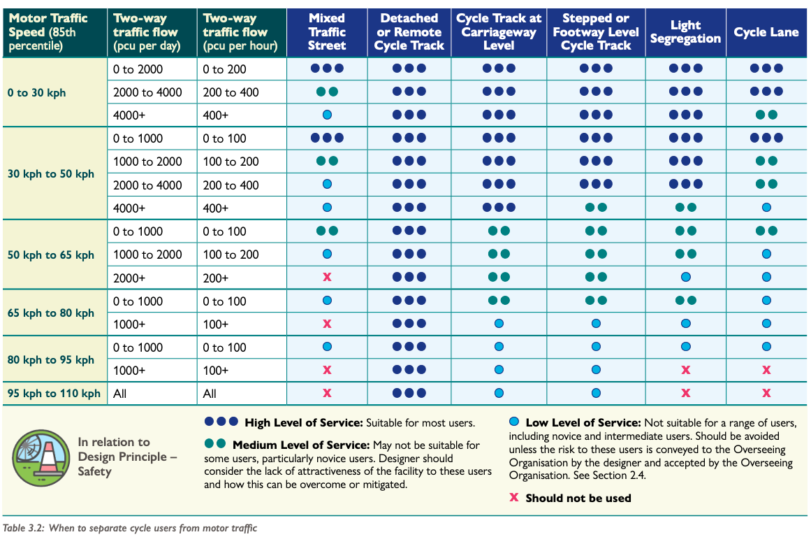
35 |
36 |
37 |
38 | ```{r}
39 | #| eval: false
40 | #| echo: false
41 | #| label: update-los-table
42 | # NOTE: run this locally
43 | devtools::load_all()
44 | # table(cycle_net$cycle_segregation)
45 | # Segregated Track (wide) Off Road Path Segregated Track (narrow)
46 | # 214 973 859
47 | # Shared Footway Painted Cycle Lane
48 | # 3325 522
49 | los_table = read_csv("https://github.com/nptscot/osmactive/raw/refs/heads/main/inst/extdata/level-of-service-table.csv")
50 |
51 | # names(los_table)
52 | # [1] "Motor Traffic Speed (85th percentile)"
53 | # [2] "Speed Limit (mph)"
54 | # [3] "Speed Limit (kph)"
55 | # [4] "Two-way traffic flow (pcu per day)"
56 | # [5] "Two-way traffic flow (pcu per hour)"
57 | # [6] "Mixed Traffic Street"
58 | # [7] "Detached or Remote Cycle Track"
59 | # [8] "Cycle Track at Carriageway Level"
60 | # [9] "Stepped or Footway Level Cycle Track"
61 | # [10] "Light Segregation"
62 | # [11] "Cycle Lane"
63 |
64 |
65 | los_table_npt = los_table |>
66 | transmute(
67 | `Speed (85th kph)` = `Motor Traffic Speed (85th percentile)`,
68 | `Speed Limit (mph)` = `Speed Limit (mph)`,
69 | `Speed Limit (kph)` = `Speed Limit (kph)`,
70 | `AADT` = `Two-way traffic flow (pcu per day)`,
71 | `Mixed Traffic Street`,
72 | `Off Road Path` = `Detached or Remote Cycle Track`,
73 | `Segregated Track (wide)` = `Cycle Track at Carriageway Level`,
74 | `Segregated Track (narrow)` = `Light Segregation`,
75 | `Painted Cycle Lane` = `Cycle Lane`
76 | ) |>
77 | # Convert the categories to "0 to 1999", "2000 to 3999", "4000+"
78 | mutate(
79 | AADT = npt_to_cbd_aadt(AADT)
80 | )
81 |
82 | los_table_complete = los_table_npt |>
83 | pivot_longer(
84 | cols = c("Mixed Traffic Street",
85 | "Off Road Path",
86 | "Segregated Track (wide)",
87 | "Segregated Track (narrow)",
88 | "Painted Cycle Lane"),
89 | names_to = "infrastructure",
90 | values_to = "level_of_service"
91 | )
92 |
93 | write_csv(los_table_complete, "inst/extdata/los_table_complete.csv")
94 | usethis::use_data(los_table_complete, overwrite = TRUE)
95 | ```
96 |
97 | # Testing the classification
98 |
99 | ```{r}
100 | osm_net = osmactive::get_travel_network("Edinburgh") |> st_transform(crs = 27700)
101 | zone = zonebuilder::zb_zone("edinburgh", n_circles = 3) |> st_transform(crs = 27700)
102 | osm_net = osm_net[zone, ]
103 | osm = osmactive::get_cycling_network(osm_net)
104 | cycle_net = get_cycling_network(osm)
105 | drive_net = get_driving_network(osm)
106 | drive_net_major = get_driving_network(osm)
107 | cycle_net = distance_to_road(cycle_net, drive_net)
108 | cycle_net = classify_cycle_infrastructure(cycle_net)
109 | table(cycle_net$detailed_segregation)
110 | table(cycle_net$cycle_segregation)
111 | ```
112 |
113 |
114 | We can then create the `Speed Limit (mph)` and `AADT` columns in the `cycle_net` object:
115 |
116 | ```{r}
117 | print("Original maxspeed for residential:")
118 | unique((cycle_net |> filter(highway == "residential"))$maxspeed)
119 | print("Original maxspeed for service:")
120 | unique((cycle_net |> filter(highway == "service"))$maxspeed)
121 |
122 | cycle_net_speeds = clean_speeds(cycle_net)
123 | unique((cycle_net_speeds |> filter(highway == "residential"))$maxspeed_clean)
124 | unique((cycle_net_speeds |> filter(highway == "service"))$maxspeed_clean)
125 |
126 | cycle_net_volumes = estimate_traffic(cycle_net_speeds)
127 | cycle_net$`Speed Limit (mph)` = classify_speeds(cycle_net_speeds$maxspeed_clean)
128 | cycle_net$AADT = npt_to_cbd_aadt_numeric(cycle_net_volumes$assumed_volume)
129 | table(cycle_net$`Speed Limit (mph)`)
130 | table(cycle_net$AADT)
131 | ```
132 |
133 |
134 | ```{r}
135 | #| eval: false
136 | #| echo: false
137 | # table(los_table_long$`Speed Limit (mph)`)
138 | # <20 mph 20 mph 30 mph 40 mph 50 mph 60+ mph
139 | # 12 16 12 8 8 4
140 | cycle_net_speeds = clean_speeds(cycle_net)
141 | # table(cycle_net_speeds$maxspeed_clean)
142 | # 15 20 30 40 50 60
143 | # 1 314 239 92 2 22
144 | classify_speeds = function(speed_mph) {
145 | dplyr::case_when(
146 | speed_mph < 20 ~ "<20 mph",
147 | speed_mph < 30 ~ "20 mph",
148 | speed_mph < 40 ~ "30 mph",
149 | speed_mph < 50 ~ "40 mph",
150 | speed_mph < 60 ~ "50 mph",
151 | speed_mph >= 60 ~ "60+ mph"
152 | )
153 | }
154 | classify_speeds(30)
155 | classify_speeds(10)
156 | classify_speeds(NA)
157 | ```
158 |
159 | ```{r minimal_plot_osm}
160 | m = plot_osm_tmap(cycle_net)
161 | m
162 | ```
163 |
164 | Let's try running the code on a larger example, covering Edinburgh:
165 |
166 | but let's solve speed NA problem in cycle_net first:
167 |
168 | ```{r}
169 | devtools::load_all() # load minimal exmaple cycle_net_f and drive_net_f
170 | cycle_net = cycle_net_f
171 | drive_net = drive_net_f
172 | mapview::mapview(cycle_net, color = "blue") +
173 | mapview::mapview(drive_net, color = "red")
174 |
175 | cycle_net$maxspeed
176 | # Stplanr function:
177 | stplanr::line_bearing(cycle_net)
178 | # All values between -90 and 90 degrees
179 | stplanr::line_bearing(cycle_net, bidirectional = TRUE)
180 |
181 | # TODO: check implementations
182 | find_nearby_speeds = function(cycle_net, drive_net, buffer_dist = 10, angle_threshold = 20) {
183 | infra_no_maxspeed = cycle_net |>
184 | filter(is.na(maxspeed))
185 |
186 | infra_no_maxspeed$azimuth_cycle =
187 | stplanr::line_bearing(infra_no_maxspeed, bidirectional = TRUE)
188 |
189 | # This should be a small datasets so OK to buffer:
190 | infra_no_maxspeed_buffer = sf::st_buffer(infra_no_maxspeed, dist = buffer_dist)
191 |
192 | roads_with_maxspeed = drive_net |>
193 | filter(!is.na(maxspeed))
194 |
195 | roads_with_maxspeed$azimuth_road =
196 | stplanr::line_bearing(roads_with_maxspeed, bidirectional = TRUE)
197 |
198 | roads_with_maxspeed_points = sf::st_point_on_surface(roads_with_maxspeed)
199 | infra_no_maxspeed_nearby = infra_no_maxspeed_buffer[roads_with_maxspeed_points, ]
200 |
201 | joined_data = sf::st_join(
202 | infra_no_maxspeed_nearby |>
203 | dplyr::select(osm_id, azimuth_cycle),
204 | roads_with_maxspeed_points |>
205 | dplyr::select(maxspeed, azimuth_road),
206 | join = sf::st_intersects
207 | )
208 |
209 | joined_data_clean = joined_data |>
210 | sf::st_drop_geometry() |>
211 | mutate(
212 | angle_diff = abs(azimuth_cycle - azimuth_road),
213 | maxspeed_numeric = gsub(maxspeed, pattern = " mph", replacement = "") |>
214 | as.numeric()
215 | ) |>
216 | filter(angle_diff < angle_threshold) |>
217 | group_by(osm_id) |>
218 | dplyr::summarise(
219 | maxspeed_new = median(maxspeed_numeric, na.rm = TRUE) |>
220 | paste0(" mph")
221 | ) |>
222 | ungroup()
223 |
224 | cycle_net_joined = left_join(
225 | cycle_net,
226 | joined_data_clean |>
227 | dplyr::select(osm_id, maxspeed_new),
228 | ) |>
229 | mutate(
230 | maxspeed = case_when(
231 | is.na(maxspeed) ~ maxspeed_new,
232 | TRUE ~ maxspeed
233 | )
234 | ) |>
235 | select(-maxspeed_new)
236 |
237 |
238 | return(cycle_net_joined)
239 | }
240 |
241 | cycle_net_f_updated = find_nearby_speeds(cycle_net_f, drive_net_f)
242 |
243 | mapview(cycle_net_f_updated, zcol = "maxspeed")
244 |
245 |
246 | # Number of rows with NA maxspeed, before:
247 | sum(is.na(cycle_net_f$maxspeed))
248 | sum(is.na(cycle_net_f_updated$maxspeed))
249 | # We've reduced the number of NAs from 28 to 20 in the test dataset
250 | ```
251 |
252 | ```{r}
253 | # testing new get_parallel_values() function
254 | devtools::load_all()
255 | target_net = cycle_net_f
256 | source_net = drive_net_f
257 | cycle_net_f_updated2 = get_parallel_values(
258 | cycle_net,
259 | drive_net,
260 | buffer_dist = 10,
261 | angle_threshold = 20
262 | )
263 |
264 | # Check the number of NAs after imputation
265 | sum(is.na(cycle_net_f_updated2$maxspeed))
266 | # Check the number of NAs before imputation
267 | sum(is.na(cycle_net_f$maxspeed))
268 | ```
269 |
270 |
271 | ```{r edinburgh}
272 | osm = get_travel_network("Edinburgh")
273 | cycle_net = get_cycling_network(osm)
274 | drive_net = get_driving_network(osm)
275 |
276 | joined_data = find_nearby_speeds(cycle_net, drive_net)
277 | cycle_net = update_missing_speeds(cycle_net, joined_data)
278 |
279 | mapview(cycle_net[central_edinburgh, ], zcol = "maxspeed")
280 |
281 | cycle_net = distance_to_road(cycle_net, drive_net)
282 | cycle_net = classify_cycle_infrastructure(cycle_net)
283 | mapview::mapview(cycle_net |>select(geometry, cycle_segregation), zcol = "cycle_segregation")
284 | central_edinburgh = osm_edinburgh |>
285 | sf::st_union() |>
286 | sf::st_centroid() |>
287 | sf::st_buffer(3000)
288 | m = plot_osm_tmap(cycle_net[central_edinburgh, ])
289 | m
290 | ```
291 |
292 | We can pick out specific bits of infrastructure, e.g. those mentioned in issue [#67](https://github.com/nptscot/osmactive/issues/67):
293 |
294 | > https://www.openstreetmap.org/way/1137759929 shows up as this right now, but this looks like a narrow segregated / stepped track to me. https://www.openstreetmap.org/way/1209807768 is another case that doesn't seem like off-road.
295 |
296 | > My idea of off-road cycleway were things like https://www.openstreetmap.org/way/7973833 and https://www.openstreetmap.org/way/265320503 -- things with no parallel road nearby.
297 |
298 | Let's pull out those bits of infrastructure:
299 |
300 | ```{r}
301 | cycle_net_included = cycle_net |>
302 | subset(osm_id %in% c(1137759929, 1209807768, 7973833, 265320503))
303 | names(cycle_net_included)
304 | cycle_net_included[c("osm_id", "distance_to_road", "cycle_segregation")] |>
305 | sf::st_drop_geometry() |>
306 | knitr::kable()
307 | ```
308 |
309 | We can also plot these as follows:
310 |
311 | ```{r}
312 | m = plot_osm_tmap(cycle_net_included)
313 | m
314 | ```
315 |
316 | ## Tests for Leith Walk
317 |
318 | ```{r}
319 | drive_net_speeds = clean_speeds(drive_net)
320 | # Check for Leith Walk
321 | drive_net_speeds |>
322 | filter(name == "Leith Walk") |>
323 | select(matches("speed"))
324 | ```
325 |
326 | ```{r}
327 | # devtools::load_all()
328 | cycle_net_los = level_of_service(cycle_net)
329 | # |>
330 | # select(osm_id, `Level of Service`, `Speed Limit (mph)`, AADT, cycle_segregation)
331 | table(cycle_net_los$`Level of Service`)
332 | # Count NA values:
333 | cycle_net_los |>
334 | sf::st_drop_geometry() |>
335 | group_by(`Speed Limit (mph)`, AADT, cycle_segregation) |>
336 | summarise(na = sum(is.na(`Level of Service`))) |>
337 | filter(na > 0) |>
338 | arrange(desc(na))
339 | cycle_net_los_plot = cycle_net_los |>
340 | select(osm_id, `Speed Limit (mph)`, AADT, cycle_segregation, `Level of Service`)
341 | mapview::mapview(cycle_net_los, zcol = "Level of Service")
342 | ```
343 |
344 | ```{r}
345 | #| eval: false
346 | #| echo: false
347 | # Try for Leeds
348 | devtools::load_all()
349 | osm = get_travel_network("Leeds")
350 | cycle_net = get_cycling_network(osm)
351 | drive_net = get_driving_network(osm)
352 | cycle_net = distance_to_road(cycle_net, drive_net)
353 | cycle_net = classify_cycle_infrastructure(cycle_net, include_mixed_traffic = TRUE)
354 | # Add aadt and speed limit
355 | cycle_net_speeds = clean_speeds(cycle_net)
356 | cycle_net = estimate_traffic(cycle_net_speeds)
357 | # Classify volumes:
358 | cycle_net$AADT = npt_to_cbd_aadt_numeric(cycle_net$assumed_volume)
359 | cycle_net$`Speed Limit (mph)` = classify_speeds(cycle_net_speeds$maxspeed_clean)
360 | names(cycle_net_speeds)
361 | cycle_net_los = level_of_service(cycle_net)
362 | # mapview::mapview(cycle_net_los, zcol = "Level of Service")
363 | table(cycle_net_los$`Level of Service`)
364 |
365 | chapeltown_area = zonebuilder::zb_zone("Chapeltown, Leeds", n_circles = 3)
366 | cycle_net_los_ctown = cycle_net_los |>
367 | sf::st_filter(chapeltown_area) |>
368 | select(osm_id, highway, `Speed Limit (mph)`, AADT, cycle_segregation, `Level of Service`)
369 | nrow(cycle_net_los_ctown)
370 | mapview::mapview(cycle_net_los_ctown, zcol = "Level of Service")
371 | # Check non-compliant ones
372 | cycle_net_los_ctown |>
373 | filter(`Level of Service` == "Should not be used (non-compliant intervention)") |>
374 | mapview::mapview(zcol = "Level of Service")
375 | ```
376 |
377 | ```{r}
378 | #| eval: false
379 | #| echo: false
380 | # check the clean_speeds function
381 | library(dplyr)
382 | library(sf)
383 |
384 | cycle_net_df = st_drop_geometry(cycle_net)
385 |
386 | # Summarize the original data (rows with missing maxspeed)
387 | original_na_summary = cycle_net_df |>
388 | filter(is.na(maxspeed)) |>
389 | group_by(highway) |>
390 | summarise(count_before = n())
391 |
392 | # Filter rows with missing maxspeed and apply the cleaning function
393 | cycle_net_na = cycle_net_df |> filter(is.na(maxspeed))
394 | unique(cycle_net_speeds$highway)
395 | # [1] "residential" "tertiary" "service" "secondary"
396 | # [5] "unclassified" "footway" "primary" "trunk"
397 | # [9] "cycleway" "pedestrian" "path" "living_street"
398 | # [13] "trunk_link" "secondary_link" "primary_link" "tertiary_link"
399 | # [17] "busway" "razed"
400 | cycle_net_speeds = clean_speeds(cycle_net_na)
401 |
402 | # Drop geometry from the cleaned data as well
403 | cycle_net_speeds_df = st_drop_geometry(cycle_net_speeds)
404 |
405 | # Summarize the cleaned data, using maxspeed_clean (the updated speed)
406 | cleaned_summary = cycle_net_speeds_df |>
407 | group_by(highway) |>
408 | summarise(
409 | updated_speed = first(maxspeed_clean),
410 | count_after = n()
411 | )
412 |
413 | # Join the before and after summaries to compare
414 | comparison = left_join(original_na_summary, cleaned_summary, by = "highway")
415 |
416 | print(comparison)
417 | ```
418 |
419 |
--------------------------------------------------------------------------------
/vignettes/gisruk2025.Rmd:
--------------------------------------------------------------------------------
1 | ---
2 | # conference: GISRUK 2025
3 | title: "Mapping, classifying, and integrating diverse street network datasets: new methods and open source tools for active travel planning"
4 | author:
5 | - name: Robin Lovelace
6 | affiliation: Leeds Institute for Transport Studies, University of Leeds, UK
7 | orcid: 0000-0001-5679-6536
8 | - name: Zhao Wang
9 | affiliation: Leeds Institute for Transport Studies, University of Leeds, UK
10 | orcid: 0000-0002-4054-0533
11 | - name: Hussein Mahfouz
12 | affiliation: Leeds Institute for Transport Studies, University of Leeds, UK
13 | orcid: 0000-0002-6043-8616
14 | - name: Juan Pablo Fonseca Zamora
15 | affiliation: Leeds Institute for Transport Studies, University of Leeds, UK
16 | orcid: 0009-0006-7042-3828
17 | - name: Angus Calder
18 | affiliation: Sustrans Scotland
19 | - name: Martin Lucas-Smith
20 | affiliation: CycleStreets Ltd, Cambridge, UK
21 | - name: Dustin Carlino
22 | affiliation: Alan Turing Institute, London, UK
23 | orcid: 0000-0002-5565-0989
24 | - name: Josiah Parry
25 | affiliation: Environmental Systems Research Institute (Esri), Redlands, CA, USA
26 | orcid: 0000-0001-9910-865X
27 | - name: Rosa Félix
28 | affiliation: University of Lisbon
29 | orcid: 0000-0002-5642-6006
30 | # abstract: |
31 | # Evidence on street networks and their potential changes under future scenarios is crucial for active travel planning. However, most active travel models rely on oversimplified street representations, using single variables like 'quietness', neglecting key factors such as footway widths. This paper introduces new methods for classifying street networks for active travel, integrating diverse datasets from OpenStreetMap and official sources. Implemented in open source software packages `osmactive` and `anime`, these methods are scalable and reproducible. The results are showcased in a web application hosted at www.npt.scot, demonstrating how geographic data science can drive high-impact research.
32 | # # implemented in open source software packages including `osmactive` R package and the `anime` Rust crate
33 | # keywords: [network analysis, transport planning, OpenStreetMap, active travel, reproducible research]
34 | # execute:
35 | # echo: false
36 | # message: false
37 | # warning: false
38 | # eval: false
39 | # # format: gfm
40 | # # quarto add sdesabbata/quarto-gisruk
41 | # format:
42 | # gisruk-pdf:
43 | # keep-tex: true
44 | # bibliography: references.bib
45 | output: rmarkdown::html_vignette
46 | vignette: >
47 | %\VignetteIndexEntry{Mapping, classifying, and integrating diverse street network datasets: new methods and open source tools for active travel planning}
48 | %\VignetteEngine{knitr::rmarkdown}
49 | %\VignetteEncoding{UTF-8}
50 | ---
51 |
52 |
53 |
54 |
55 |
56 | ```{r}
57 | #| echo: false
58 | knitr::opts_chunk$set(eval = FALSE)
59 | ```
60 |
61 | ```{r}
62 | #| include: false
63 | # install pak if not installed:
64 | if (!requireNamespace("pak", quietly = TRUE)) {
65 | install.packages("pak")
66 | }
67 | pak::pkg_install("tidyverse", ask = FALSE)
68 |
69 | github_pkgs = c(
70 | "nptscot/osmactive",
71 | "josiahparry/anime/r"
72 | )
73 | pak::pkg_install(github_pkgs, ask = FALSE)
74 | library(tidyverse)
75 | library(osmactive)
76 | library(tmap)
77 | ```
78 |
79 |
80 |
81 |
82 |
83 | ```{r}
84 | #| eval: false
85 | #| echo: false
86 | quarto::quarto_render("os_blog_post.qmd", output_format = "docx")
87 | d = list.dirs("~/..")
88 | d_onedrive = d[grep("OneDrive", d)]
89 | list.files("~/OneDrive/projects-all/atumscotland/phase3")
90 | # file.copy("os_blog_post.docx", "~/OneDrive/projects-all/atumscotland/phase3", overwrite = TRUE)
91 | list.files( "C:\\Users\\georl_admin\\OneDrive - University of Leeds\\projects-all\\atumscotland\\phase3")
92 | file.copy("os_blog_post.docx", "C:\\Users\\georl_admin\\OneDrive - University of Leeds\\projects-all\\atumscotland\\phase3", overwrite = TRUE)
93 | # Upload to gh
94 | quarto::quarto_render("gisruk2025.qmd")
95 | system("gh release upload v0.1 gisruk2025.pdf --clobber")
96 | ```
97 |
98 | # Published versions
99 |
100 | See the [pdf version](https://github.com/nptscot/osmactive/releases/download/v0.1/gisruk2025.pdf) and [html version](https://nptscot.github.io/osmactive/articles/gisruk2025.html) at [nptscot.github.io/osmactive](https://nptscot.github.io/osmactive/articles/gisruk2025.html).
101 |
102 |
103 | # Introduction
104 |
105 | Active travel is an accessible and cost-effective way to replace short car trips and make transport systems more sustainable.
106 | The Network Planning Tool (NPT) for Scotland is a new web-based strategic network planning tool that estimates cycling potential down to the street level.
107 | The NPT builds on the functionality of the Propensity to Cycle Tool (PCT) and related tools [@lovelace2017; @goodman2019; @lovelace2024; @félix2025], offering a detailed nationwide cycling potential analysis for Scotland.
108 | The NPT is funded by Transport Scotland and developed by the University of Leeds in collaboration with Sustrans Scotland.
109 | The tool is open-source and hosted at [github.come/nptscot](https://github.com/nptscot), enabling others to learn from and contribute to the underlying methods to help make transport planning more open and participatory [@lovelace2020a].
110 |
111 | A unique feature of the NPT is its integration of multiple layers into a single tool, overcoming limitations of previous strategic network planning tools, which generally focus either on behaviour data (such as the PCT) or physical infrastructure [@vybornova2024; @vierø2024].
112 | The NPT brings together more than a dozen datasets, including Ordnance Survey Mastermap and OpenStreetmap data products to provide comprehensive data on the potential for mode shift, infrastructure, modelled motor traffic levels, and street space at the network level.
113 | This paper presents new geographic methods we developed to support this work, with reference to reproducible code that use the new `osmactive` R package for classifying national-scale OpenStreetMap (OSM) datasets based on attributes and geographic relationships, and the `anime` Rust crate for astonishingly fast and accurate route network data integration.
114 |
115 | # Datasets and methods
116 |
117 | The NPT uses datasets from diverse sources including from the DfT's network of traffic sensors, motor traffic counts based a survey evaluating Edinburgh's roll-out of 20 mph speed limits, the National Travel Survey, and the Scottish Household Travel Survey.
118 | We used four key datasets representing the road network for this project:
119 |
120 | - Ordnance Survey OpenRoads, an open access and simplified representation of the road network that is ideal for visualisation
121 | - OS MasterMap Highways, a more detailed dataset that includes information on road widths and other features
122 | - OS Mastermap Topography, the most detailed vector dataset that includes detailed information on the geometry of many features of the man-made environment, including curb lines. In the OS Topo layer roads and other pieces of transport infrastructure such as footways (pavements) are represented not as corridor or lane centerlines, but as polygons.
123 | - OpenStreetMap, a crowdsourced dataset that is continuously updated by community volunteers. The dataset is rich, with tags for width and smoothness of infrastructure, but is not as consistent as the OS datasets.
124 |
125 | Ordnance Survey's MasterMap Highways and Topography datasets provide unparalleled accuracy and detail, but are a struggle to import using consumer-grade hardware and standard tools such as QGIS.
126 | To overcome this issue we developed [the `mastermapr` package](https://github.com/acteng/mastermapr) in collaboration with the government agency Active Travel England (ATE), to efficiently and flexibly imports MasterMap datasets (50 GB compressed).
127 | After importing the four route network datasets outlined above, we integrated them using the following steps:
128 |
129 | - Pavement widths were calculated from the OS MasterMap Topography dataset using the function `get_pavement_widths()` from the `osmactive` package. This function calculates the width of manmade roadside features associated with each road segment by dividing the area of matching polygons associated with each road segment by the length of the road segment.
130 | - The `get_bus_routes()` function from the `osmactive` package was used to determine the number of bus lanes on each road segment.
131 | - We used the `anime` Rust crate to efficiently join the networks, based on alignment and proximity. The use of spatial indexes makes the implementation highly efficient compared with the [`rnet_join()`](https://docs.ropensci.org/stplanr/reference/rnet_join.html) function in the R package `stplanr` that we were using previously. See the [josiahparry/ANIME codebase on GitHub](https://github.com/JosiahParry/anime) for details of the new algorithm and its implementation as an R (and planned Python) interface to the new [`anime` Rust crate](https://crates.io/crates/anime).
132 |
133 | ## Classifying OpenStreetNetwork ways
134 |
135 | Functions including `get_travel_network()` and `classify_cycle_infrastructure()` from the `osmactive` package were used to classify cycle infrastructure types based on the presence of cycle lanes, tracks, and other features (see the code snippet which generates @fig-bristol below).
136 |
137 | ```{r}
138 | #| label: bristol
139 | #| eval: false
140 | #| echo: true
141 | osm = get_travel_network("bristol")
142 | cycle_net = get_cycling_network(osm)
143 | drive_net = get_driving_network(osm)
144 | cycle_net = distance_to_road(cycle_net, drive_net)
145 | cycle_net = classify_cycle_infrastructure(cycle_net)
146 | plot_osm_tmap(cycle_net)
147 | ```
148 |
149 |
150 |
151 | ```{r}
152 | #| include: false
153 | #| eval: false
154 | m = plot_osm_tmap(cycle_net)
155 | m +
156 | tm_layout(legend.position = c("right", "top"))
157 | m
158 | tmap_save(m, "cycle_net_bristol.html")
159 | browseURL("cycle_net_bristol.html")
160 | system("gh release upload v0.1 cycle_net_bristol.html --clobber")
161 | # Available:
162 | # https://github.com/nptscot/osmactive/releases/download/v0.1/cycle_net_bristol.html
163 | ```
164 |
165 | .](images/paste-1.png){#fig-bristol}
166 |
167 | ## Road width measurements
168 |
169 | Two key measurements are needed to assess whether existing roads can accommodate cycle infrastructure: carriageway width and corridor width, as defined below.
170 |
171 | Accurate and available carriageway width measurements are important because they determine if proposed infrastructure can fit solely within the carriageway, without the need for moving curbs or other roadside features.
172 | The Scottish Cycling by Design (CbD) guidance document outlines three types of cycle infrastructure that run along the carriageway, building on Department for Transport guidance [@departmentfortransport2020]:
173 |
174 | - Cycle track at carriageway level
175 | - Stepped cycle track
176 | - Cycle track at footway level
177 |
178 | The first option, cycle track that is at carriage level, has additional advantages over stepped cycleway, being often cheaper to construct [with no new tarmac required in many cases](https://www.transport.gov.scot/media/50323/cycling-by-design-update-2019-final-document-15-september-2021-1.pdf#page=76) but requires sufficient width on the existing carriageway to accommodate the cycle infrastructure.
179 |
180 | Corridor width captures the carriageway plus any built roadside features, such as footways.
181 | The following [`dplyr` query](https://dplyr.tidyverse.org/) was used to extract the width of manmade roadside features: `filter(descriptive_group == "Roadside", make == "Manmade")`.
182 | From that point, we calculated the width of pavements associated with each road segment by dividing the area of matching polygons associated with each road segment by the length of the road segment, as implemented in the `get_pavement_widths()` function in the `osmactive` package.
183 |
184 | ## Minimum cycle track and buffer widths
185 |
186 | The corridor width is important because it determines whether, in cases where there is insufficient space on the carriageway, part of the footway or other manmade roadside features may be reallocated for cycle infrastructure, while still maintaining recommended minimum widths for pedestrians.
187 | CbD guidance on widths is summarised in table @tbl-cbd.
188 |
189 | | Cycle infrastructure type | Absolute minimum width | Desirable minimum width |
190 | |--------------------------|-----------------------|------------------------|
191 | | Unidirectional cycle track | 1.5 m | 2.0 m |
192 | | Bidirectional cycle track | 2.0 m | 3.0 m |
193 |
194 | : Table illustrating the minimum width requirements for cycle infrastructure according to the Cycling by Design (CbD) guidance. {#tbl-cbd}
195 |
196 | CbD also specifies buffers that must be accounted for when calculating the effective available width for cycle infrastructure (@tbl-buffers).
197 |
198 | | Road type / Speed limit | Buffer width |
199 | |-------------------------|--------------|
200 | | 30 mph | 0.5 m |
201 | | 40 mph | 1.0 m |
202 | | 50 mph | 2.0 m |
203 | | 60 mph | 2.5 m |
204 | | 70 mph | 3.5 m |
205 |
206 | : Table illustrating the buffer widths for cycle infrastructure based on road type and speed limit according to the Cycling by Design (CbD) guidance. {#tbl-buffers}
207 |
208 | Speed limit data taken from OSM was used to determine the buffer width for each road segment.
209 |
210 | ## Bus routes and road traffic assumptions
211 |
212 | The minimum space requirements for motor traffic depend on the uses of the road, including whether it is a bus route and whether there are dedicated bus lanes.
213 | Based on the Active Travel England cross section check tool, part of [Active Travel England's open access Excel-based design tools](https://www.gov.uk/government/publications/active-travel-england-design-assistance-tools) (see [acteng.github.io/inspectorate_tools/](https://acteng.github.io/inspectorate_tools/) for web-based versions), we assumed the following widths for motor traffic:
214 |
215 | - Non-bus routes: 2 × 2.75 m
216 | - Bus routes without dedicated bus lanes: 2 × 3.2 m
217 | - Bus routes with dedicated bus lanes: 2 × 3.2 m plus an additional space of `n_bus_lanes` × 3.2 m for the dedicated bus lanes.
218 |
219 |
220 |
221 | The number of bus lanes was determined from the OSM data with the function [`get_bus_routes()`](https://nptscot.github.io/osmactive/reference/get_bus_routes.html) in the R package `osmactive` that we developed for this project.
222 | The results are illustrated in @fig-edinburgh-bus-lanes, which can also be reproduced with the following [Overpass Turbo query](https://overpass-turbo.eu/s/1Xaf):
223 |
224 | ```
225 | relation["route"="bus"]({{bbox}});
226 | ```
227 |
228 |
229 |
230 |
231 |
232 |
233 |
234 |
235 |
236 | # Results
237 |
238 | The result of the data engineering, data integration, modelling and visualisation steps described above is datasets that are visualised interactively in the NPT web application, using `pmtiles` for efficient rendering of large datasets [@gonçalves2023].
239 | The key components of the NPT are:
240 |
241 | - The "Route network" layer, presenting data on cycling potential on OSM-based and simplified [@lovelace_reproducible_2024] network layers.
242 | - The "Infrastructure and traffic" layer, which includes data on motor traffic levels and cycle infrastructure.
243 | - The "Street space" layer, which categorises roads in accordance with the Cycling by Design guidance, specifying the methodology for classifying road spaces and cycle infrastructure, presented in @fig-street-space.
244 | - The "Core network" layer, representing a cohesive network that could be a priority when planning new infrastructure, building on previous work [@szell2021].
245 | - The [Network Planning Workspace (NPW)](https://nptscot.github.io/npw/) web application, which allows users to explore the data and create custom scenarios of infrastructure change.
246 |
247 |
248 |
249 |
250 |
251 | # Conclusion
252 |
253 | The Network Planning Tool for Scotland is a cutting-edge web application designed for strategic cycle network planning.
254 | A unique feature of the NPT is its integration of multiple layers into a single tool, overcoming limitations of previous strategic network planning tools, which generally focus either on behaviour data or physical infrastructure.
255 | The new street space layer represents a step change in access to combined carriageway and corridor widths, the first time this data has been made available at a national level, to the best of our knowledge.
256 |
257 | In future work we plan to improve the NPT by incorporating new datasets from a variety of sources, including [Scotland's Spatial Hub](https://data.spatialhub.scot).
258 | We would like to develop context-specific classifications in the `osmactive` package to better address the diverse needs of different urban environments and support the roll-out the methods in new places.
259 |
260 | # References
261 |
262 | ::: {#refs}
263 | :::
264 |
265 | # Acknowledgements {.appendix .unnumbered}
266 |
267 |
268 |
269 | Thanks to Transport Scotland for funding the development of the Network Planning Tool for Scotland, and to the many users who have provided feedback on the tool.
270 | Thanks to Sustrans Scotland, and Matt Davis and Angus Calder in particular, for collaborating on the project.
271 |
272 | Thanks to the OpenStreetMap community for creating and maintaining the data that underpins the NPT.
273 | Thanks to Ordnance Survey for providing the MasterMap data that underpins the NPT (contains OS data © Crown copyright and database rights 2025 OS licence number 100046668).
274 |
275 | # Biographies {.appendix .unnumbered}
276 |
277 |
278 |
279 | Robin Lovelace is Professor of Transport Data Science at the Leeds Institute for Transport Studies (ITS) and specialises in data science and geocomputation, with a focus on modeling transport systems, active travel, and decarbonisation.
280 |
281 | Zhao Wang is a researcher at the Leeds Institute for Transport Studies (ITS).
282 | Zhao specializes in machine learning, data science and geocomputation for transport planning and engineering.
283 |
284 | Hussein Mahfouz is a PhD student at the Leeds Institute for Transport Studies (ITS) and specialises in data science and geocomputation for transport planning and engineering, with a focus on Demand Responsive Transport (DRT).
285 |
286 | Juan Pablo Fonseca Zamora is a PhD student at the Leeds Institute for Transport Studies (ITS) and specialises in new methods for traffic modelling.
287 |
288 | Angus Calder is a Senior Mobility Planner at Sustrans Scotland and specialises in active travel planning and infrastructure design.
289 |
290 | Martin Lucas-Smith is a Director at CycleStreets Ltd and specialises in open data and open source software for cycling.
291 |
292 | Dustin Carlino is an independent researcher and software developer, specialising in open source software development and geographic data science.
293 |
294 | Josiah Parry is a Senior Product Engineer at Environmental Systems Research Institute, Inc (Esri) and an open source software developer.
295 |
296 | Rosa Félix is a researcher at the University of Lisbon and specialises geographic methods for transport planning, with a focus on active travel and decarbonisation.
297 |
298 | ```{=html}
299 |
308 | ```
309 |
--------------------------------------------------------------------------------
/data-raw/gisruk2025.qmd:
--------------------------------------------------------------------------------
1 | ---
2 | conference: GISRUK 2025
3 | title: "Mapping, classifying, and integrating diverse street network datasets: new methods and open source tools for active travel planning"
4 | author:
5 | - name: Robin Lovelace
6 | affiliation: Leeds Institute for Transport Studies, University of Leeds, UK
7 | orcid: 0000-0001-5679-6536
8 | - name: Zhao Wang
9 | affiliation: Leeds Institute for Transport Studies, University of Leeds, UK
10 | orcid: 0000-0002-4054-0533
11 | - name: Hussein Mahfouz
12 | affiliation: Leeds Institute for Transport Studies, University of Leeds, UK
13 | orcid: 0000-0002-6043-8616
14 | - name: Juan Pablo Fonseca Zamora
15 | affiliation: Leeds Institute for Transport Studies, University of Leeds, UK
16 | orcid: 0009-0006-7042-3828
17 | - name: Angus Calder
18 | affiliation: Sustrans Scotland
19 | - name: Martin Lucas-Smith
20 | affiliation: CycleStreets Ltd, Cambridge, UK
21 | - name: Dustin Carlino
22 | affiliation: Alan Turing Institute, London, UK
23 | orcid: 0000-0002-5565-0989
24 | - name: Josiah Parry
25 | affiliation: Environmental Systems Research Institute (Esri), Redlands, CA, USA
26 | orcid: 0000-0001-9910-865X
27 | - name: Rosa Félix
28 | affiliation: University of Lisbon
29 | orcid: 0000-0002-5642-6006
30 | abstract: |
31 | Evidence on street networks and their potential changes under future scenarios is crucial for active travel planning. However, most active travel models rely on oversimplified street representations, using single variables like 'quietness', neglecting key factors such as footway widths. This paper introduces new methods for classifying street networks for active travel, integrating diverse datasets from OpenStreetMap and official sources. Implemented in open source software packages `osmactive` and `anime`, these methods are scalable and reproducible. The results are showcased in a web application hosted at www.npt.scot, demonstrating how geographic data science can drive high-impact research.
32 | # implemented in open source software packages including `osmactive` R package and the `anime` Rust crate
33 | keywords: [network analysis, transport planning, OpenStreetMap, active travel, reproducible research]
34 | execute:
35 | echo: false
36 | message: false
37 | warning: false
38 | # eval: false
39 | # format: gfm
40 | # quarto add sdesabbata/quarto-gisruk
41 | format:
42 | gisruk-pdf:
43 | keep-tex: true
44 | bibliography: references.bib
45 | ---
46 |
47 | ```{=html}
48 |
51 | ```
52 |
53 |
54 |
55 |
56 |
57 | ```{r}
58 | #| include: false
59 | # install pak if not installed:
60 | if (!requireNamespace("pak", quietly = TRUE)) {
61 | install.packages("pak")
62 | }
63 | pak::pkg_install("tidyverse", ask = FALSE)
64 |
65 | github_pkgs = c(
66 | "nptscot/osmactive",
67 | "josiahparry/anime/r"
68 | )
69 | pak::pkg_install(github_pkgs, ask = FALSE)
70 | library(tidyverse)
71 | library(osmactive)
72 | library(tmap)
73 | ```
74 |
75 |
76 |
77 |
78 |
79 | ```{r}
80 | #| eval: false
81 | #| echo: false
82 | quarto::quarto_render("os_blog_post.qmd", output_format = "docx")
83 | d = list.dirs("~/..")
84 | d_onedrive = d[grep("OneDrive", d)]
85 | list.files("~/OneDrive/projects-all/atumscotland/phase3")
86 | # file.copy("os_blog_post.docx", "~/OneDrive/projects-all/atumscotland/phase3", overwrite = TRUE)
87 | list.files( "C:\\Users\\georl_admin\\OneDrive - University of Leeds\\projects-all\\atumscotland\\phase3")
88 | file.copy("os_blog_post.docx", "C:\\Users\\georl_admin\\OneDrive - University of Leeds\\projects-all\\atumscotland\\phase3", overwrite = TRUE)
89 | # Upload to gh
90 | quarto::quarto_render("gisruk2025.qmd")
91 | system("gh release upload v0.1 gisruk2025.pdf --clobber")
92 | ```
93 |
94 |
95 |
96 | ```{=html}
97 |
129 | ```
130 |
131 | ```{=html}
132 |
147 | ```
148 |
149 | ```{=html}
150 |
218 | ```
219 |
220 | {{< pagebreak >}}
221 |
222 | # Introduction
223 |
224 | Active travel is an accessible and cost-effective way to replace short car trips and make transport systems more sustainable.
225 | The Network Planning Tool (NPT) for Scotland is a new web-based strategic network planning tool that estimates cycling potential down to the street level.
226 | The NPT builds on the functionality of the Propensity to Cycle Tool (PCT) and related tools [@lovelace2017; @goodman2019; @lovelace2024; @félix2025], offering a detailed nationwide cycling potential analysis for Scotland.
227 | The NPT is funded by Transport Scotland and developed by the University of Leeds in collaboration with Sustrans Scotland.
228 | The tool is open-source and hosted at [github.come/nptscot](https://github.com/nptscot), enabling others to learn from and contribute to the underlying methods to help make transport planning more open and participatory [@lovelace2020a].
229 |
230 | A unique feature of the NPT is its integration of multiple layers into a single tool, overcoming limitations of previous strategic network planning tools, which generally focus either on behaviour data (such as the PCT) or physical infrastructure [@vybornova2024; @vierø2024].
231 | The NPT brings together more than a dozen datasets, including Ordnance Survey Mastermap and OpenStreetmap data products to provide comprehensive data on the potential for mode shift, infrastructure, modelled motor traffic levels, and street space at the network level.
232 | This paper presents new geographic methods we developed to support this work, with reference to reproducible code that use the new `osmactive` R package for classifying national-scale OpenStreetMap (OSM) datasets based on attributes and geographic relationships, and the `anime` Rust crate for astonishingly fast and accurate route network data integration.
233 |
234 | # Datasets and methods
235 |
236 | The NPT uses datasets from diverse sources including from the DfT's network of traffic sensors, motor traffic counts based a survey evaluating Edinburgh's roll-out of 20 mph speed limits, the National Travel Survey, and the Scottish Household Travel Survey.
237 | We used four key datasets representing the road network for this project:
238 |
239 | - Ordnance Survey OpenRoads, an open access and simplified representation of the road network that is ideal for visualisation
240 | - OS MasterMap Highways, a more detailed dataset that includes information on road widths and other features
241 | - OS Mastermap Topography, the most detailed vector dataset that includes detailed information on the geometry of many features of the man-made environment, including curb lines. In the OS Topo layer roads and other pieces of transport infrastructure such as footways (pavements) are represented not as corridor or lane centerlines, but as polygons.
242 | - OpenStreetMap, a crowdsourced dataset that is continuously updated by community volunteers. The dataset is rich, with tags for width and smoothness of infrastructure, but is not as consistent as the OS datasets.
243 |
244 | Ordnance Survey’s MasterMap Highways and Topography datasets provide unparalleled accuracy and detail, but are a struggle to import using consumer-grade hardware and standard tools such as QGIS.
245 | To overcome this issue we developed [the `mastermapr` package](https://github.com/acteng/mastermapr) in collaboration with the government agency Active Travel England (ATE), to efficiently and flexibly imports MasterMap datasets (50 GB compressed).
246 | After importing the four route network datasets outlined above, we integrated them using the following steps:
247 |
248 | - Pavement widths were calculated from the OS MasterMap Topography dataset using the function `get_pavement_widths()` from the `osmactive` package. This function calculates the width of manmade roadside features associated with each road segment by dividing the area of matching polygons associated with each road segment by the length of the road segment.
249 | - The `get_bus_routes()` function from the `osmactive` package was used to determine the number of bus lanes on each road segment.
250 | - We used the `anime` Rust crate to efficiently join the networks, based on alignment and proximity. The use of spatial indexes makes the implementation highly efficient compared with the [`rnet_join()`](https://docs.ropensci.org/stplanr/reference/rnet_join.html) function in the R package `stplanr` that we were using previously. See the [josiahparry/ANIME codebase on GitHub](https://github.com/JosiahParry/anime) for details of the new algorithm and its implementation as an R (and planned Python) interface to the new [`anime` Rust crate](https://crates.io/crates/anime).
251 |
252 | ## Classifying OpenStreetNetwork ways
253 |
254 | Functions including `get_travel_network()` and `classify_cycle_infrastructure()` from the `osmactive` package were used to classify cycle infrastructure types based on the presence of cycle lanes, tracks, and other features (see the code snippet which generates @fig-bristol below).
255 |
256 | ```{r}
257 | #| label: bristol
258 | #| eval: false
259 | #| echo: true
260 | osm = get_travel_network("bristol")
261 | cycle_net = get_cycling_network(osm)
262 | drive_net = get_driving_network(osm)
263 | cycle_net = distance_to_road(cycle_net, drive_net)
264 | cycle_net = classify_cycle_infrastructure(cycle_net)
265 | plot_osm_tmap(cycle_net)
266 | ```
267 |
268 |
269 |
270 | ```{r}
271 | #| include: false
272 | #| eval: false
273 | m = plot_osm_tmap(cycle_net)
274 | m +
275 | tm_layout(legend.position = c("right", "top"))
276 | m
277 | tmap_save(m, "cycle_net_bristol.html")
278 | browseURL("cycle_net_bristol.html")
279 | system("gh release upload v0.1 cycle_net_bristol.html --clobber")
280 | # Available:
281 | # https://github.com/nptscot/osmactive/releases/download/v0.1/cycle_net_bristol.html
282 | ```
283 |
284 | .](images/paste-1.png){#fig-bristol}
285 |
286 | ## Road width measurements
287 |
288 | Two key measurements are needed to assess whether existing roads can accommodate cycle infrastructure: carriageway width and corridor width, as defined below.
289 |
290 | Accurate and available carriageway width measurements are important because they determine if proposed infrastructure can fit solely within the carriageway, without the need for moving curbs or other roadside features.
291 | The Scottish Cycling by Design (CbD) guidance document outlines three types of cycle infrastructure that run along the carriageway, building on Department for Transport guidance [@departmentfortransport2020]:
292 |
293 | - Cycle track at carriageway level
294 | - Stepped cycle track
295 | - Cycle track at footway level
296 |
297 | The first option, cycle track that is at carriage level, has additional advantages over stepped cycleway, being often cheaper to construct [with no new tarmac required in many cases](https://www.transport.gov.scot/media/50323/cycling-by-design-update-2019-final-document-15-september-2021-1.pdf#page=76) but requires sufficient width on the existing carriageway to accommodate the cycle infrastructure.
298 |
299 | Corridor width captures the carriageway plus any built roadside features, such as footways.
300 | The following [`dplyr` query](https://dplyr.tidyverse.org/) was used to extract the width of manmade roadside features: `filter(descriptive_group == "Roadside", make == "Manmade")`.
301 | From that point, we calculated the width of pavements associated with each road segment by dividing the area of matching polygons associated with each road segment by the length of the road segment, as implemented in the `get_pavement_widths()` function in the `osmactive` package.
302 |
303 | ## Minimum cycle track and buffer widths
304 |
305 | The corridor width is important because it determines whether, in cases where there is insufficient space on the carriageway, part of the footway or other manmade roadside features may be reallocated for cycle infrastructure, while still maintaining recommended minimum widths for pedestrians.
306 | CbD guidance on widths is summarised in table @tbl-cbd.
307 |
308 | | Cycle infrastructure type | Absolute minimum width | Desirable minimum width |
309 | |--------------------------|-----------------------|------------------------|
310 | | Unidirectional cycle track | 1.5 m | 2.0 m |
311 | | Bidirectional cycle track | 2.0 m | 3.0 m |
312 |
313 | : Table illustrating the minimum width requirements for cycle infrastructure according to the Cycling by Design (CbD) guidance. {#tbl-cbd}
314 |
315 | CbD also specifies buffers that must be accounted for when calculating the effective available width for cycle infrastructure (@tbl-buffers).
316 |
317 | | Road type / Speed limit | Buffer width |
318 | |-------------------------|--------------|
319 | | 30 mph | 0.5 m |
320 | | 40 mph | 1.0 m |
321 | | 50 mph | 2.0 m |
322 | | 60 mph | 2.5 m |
323 | | 70 mph | 3.5 m |
324 |
325 | : Table illustrating the buffer widths for cycle infrastructure based on road type and speed limit according to the Cycling by Design (CbD) guidance. {#tbl-buffers}
326 |
327 | Speed limit data taken from OSM was used to determine the buffer width for each road segment.
328 |
329 | ## Bus routes and road traffic assumptions
330 |
331 | The minimum space requirements for motor traffic depend on the uses of the road, including whether it is a bus route and whether there are dedicated bus lanes.
332 | Based on the Active Travel England cross section check tool, part of [Active Travel England's open access Excel-based design tools](https://www.gov.uk/government/publications/active-travel-england-design-assistance-tools) (see [acteng.github.io/inspectorate_tools/](https://acteng.github.io/inspectorate_tools/) for web-based versions), we assumed the following widths for motor traffic:
333 |
334 | - Non-bus routes: 2 × 2.75 m
335 | - Bus routes without dedicated bus lanes: 2 × 3.2 m
336 | - Bus routes with dedicated bus lanes: 2 × 3.2 m plus an additional space of `n_bus_lanes` × 3.2 m for the dedicated bus lanes.
337 |
338 |
339 |
340 | The number of bus lanes was determined from the OSM data with the function [`get_bus_routes()`](https://nptscot.github.io/osmactive/reference/get_bus_routes.html) in the R package `osmactive` that we developed for this project.
341 | The results are illustrated in @fig-edinburgh-bus-lanes, which can also be reproduced with the following [Overpass Turbo query](https://overpass-turbo.eu/s/1Xaf):
342 |
343 | ```
344 | relation["route"="bus"]({{bbox}});
345 | ```
346 |
347 |
348 |
349 |
350 |
351 | {#fig-edinburgh-bus-lanes}
352 |
353 |
354 |
355 | # Results
356 |
357 | The result of the data engineering, data integration, modelling and visualisation steps described above is datasets that are visualised interactively in the NPT web application, using `pmtiles` for efficient rendering of large datasets [@gonçalves2023].
358 | The key components of the NPT are:
359 |
360 | - The "Route network" layer, presenting data on cycling potential on OSM-based and simplified [@lovelace_reproducible_2024] network layers.
361 | - The "Infrastructure and traffic" layer, which includes data on motor traffic levels and cycle infrastructure.
362 | - The "Street space" layer, which categorises roads in accordance with the Cycling by Design guidance, specifying the methodology for classifying road spaces and cycle infrastructure, presented in @fig-street-space.
363 | - The "Core network" layer, representing a cohesive network that could be a priority when planning new infrastructure, building on previous work [@szell2021].
364 | - The [Network Planning Workspace (NPW)](https://nptscot.github.io/npw/) web application, which allows users to explore the data and create custom scenarios of infrastructure change.
365 |
366 | {#fig-street-space}
367 |
368 |
369 |
370 | # Conclusion
371 |
372 | The Network Planning Tool for Scotland is a cutting-edge web application designed for strategic cycle network planning.
373 | A unique feature of the NPT is its integration of multiple layers into a single tool, overcoming limitations of previous strategic network planning tools, which generally focus either on behaviour data or physical infrastructure.
374 | The new street space layer represents a step change in access to combined carriageway and corridor widths, the first time this data has been made available at a national level, to the best of our knowledge.
375 |
376 | In future work we plan to improve the NPT by incorporating new datasets from a variety of sources, including [Scotland's Spatial Hub](https://data.spatialhub.scot).
377 | We would like to develop context-specific classifications in the `osmactive` package to better address the diverse needs of different urban environments and support the roll-out the methods in new places.
378 |
379 | # References
380 |
381 | ::: {#refs}
382 | :::
383 |
384 | # Acknowledgements {.appendix .unnumbered}
385 |
386 |
387 |
388 | Thanks to Transport Scotland for funding the development of the Network Planning Tool for Scotland, and to the many users who have provided feedback on the tool.
389 | Thanks to Sustrans Scotland, and Matt Davis and Angus Calder in particular, for collaborating on the project.
390 |
391 | Thanks to the OpenStreetMap community for creating and maintaining the data that underpins the NPT.
392 | Thanks to Ordnance Survey for providing the MasterMap data that underpins the NPT (contains OS data © Crown copyright and database rights 2025 OS licence number 100046668).
393 |
394 | # Biographies {.appendix .unnumbered}
395 |
396 |
397 |
398 | Robin Lovelace is Professor of Transport Data Science at the Leeds Institute for Transport Studies (ITS) and specialises in data science and geocomputation, with a focus on modeling transport systems, active travel, and decarbonisation.
399 |
400 | Zhao Wang is a researcher at the Leeds Institute for Transport Studies (ITS).
401 | Zhao specializes in machine learning, data science and geocomputation for transport planning and engineering.
402 |
403 | Hussein Mahfouz is a PhD student at the Leeds Institute for Transport Studies (ITS) and specialises in data science and geocomputation for transport planning and engineering, with a focus on Demand Responsive Transport (DRT).
404 |
405 | Juan Pablo Fonseca Zamora is a PhD student at the Leeds Institute for Transport Studies (ITS) and specialises in new methods for traffic modelling.
406 |
407 | Angus Calder is a Senior Mobility Planner at Sustrans Scotland and specialises in active travel planning and infrastructure design.
408 |
409 | Martin Lucas-Smith is a Director at CycleStreets Ltd and specialises in open data and open source software for cycling.
410 |
411 | Dustin Carlino is an independent researcher and software developer, specialising in open source software development and geographic data science.
412 |
413 | Josiah Parry is a Senior Product Engineer at Environmental Systems Research Institute, Inc (Esri) and an open source software developer.
414 |
415 | Rosa Félix is a researcher at the University of Lisbon and specialises geographic methods for transport planning, with a focus on active travel and decarbonisation.
416 |
417 | ```{=html}
418 |
427 | ```
--------------------------------------------------------------------------------