├── .gitignore
├── README.md
├── bike_season.png
├── bike_warhersit.png
├── bike_weekday.png
├── iml_shap_R_package.png
├── shap-post.Rmd
├── shap-values.Rproj
├── shap.R
├── shap_analysis.R
└── shap_heart_disease.R
/.gitignore:
--------------------------------------------------------------------------------
1 | .Rproj.user
2 | .Rhistory
3 | .RData
4 | .Ruserdata
5 |
--------------------------------------------------------------------------------
/README.md:
--------------------------------------------------------------------------------
1 | This repository contains the backround code of:
2 | [How to intepret SHAP values in R](https://blog.datascienceheroes.com/how-to-interpret-shap-values-in-r/)
3 |
4 |
5 | To execute this project, open and run `shap_analysis.R` (wich loads `shap.R`).
6 |
7 | It will load the `bike` dataset, do some data preparation, create a predictive model (xgboost), obtaining the SHAP values and then it will plot them:
8 |
9 |
10 |
11 | 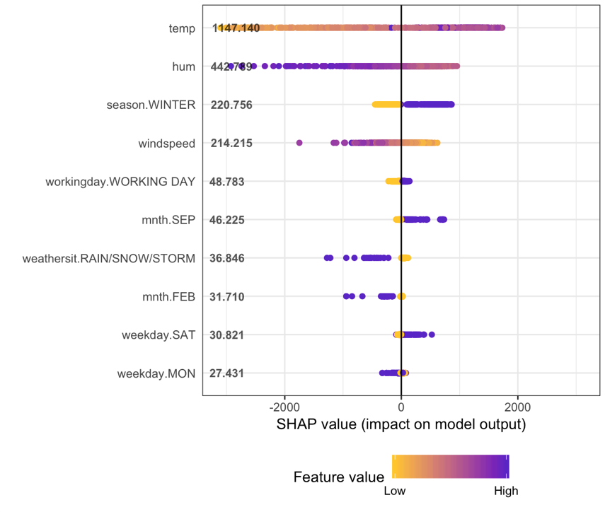 12 |
13 |
14 |
12 |
13 |
14 | 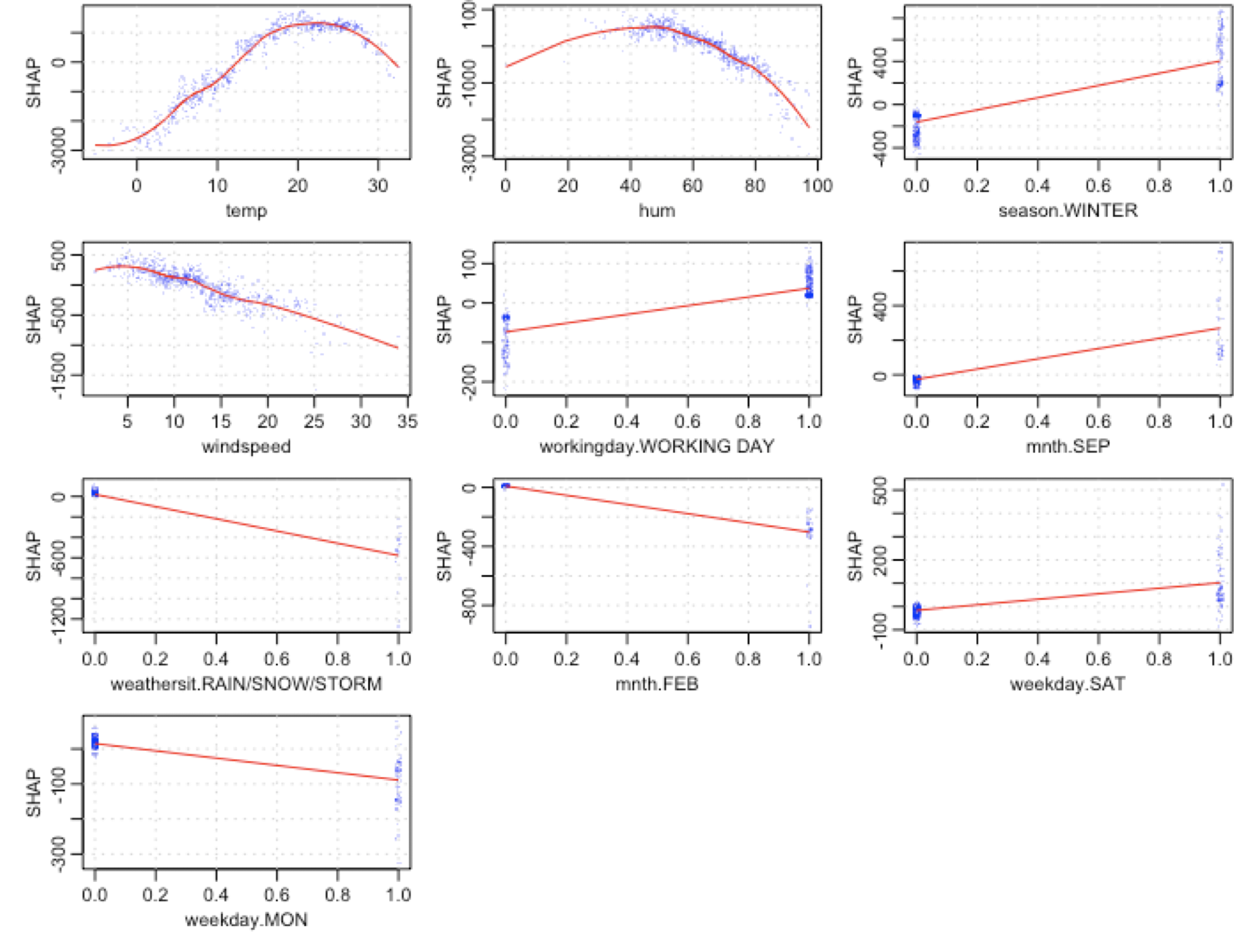 15 |
16 | It is easy to reproduce with other data. Have fun!
17 |
18 |
--------------------------------------------------------------------------------
/bike_season.png:
--------------------------------------------------------------------------------
https://raw.githubusercontent.com/pablo14/shap-values/73109cf74dd43a2e7382e703868ff6cef285ccb4/bike_season.png
--------------------------------------------------------------------------------
/bike_warhersit.png:
--------------------------------------------------------------------------------
https://raw.githubusercontent.com/pablo14/shap-values/73109cf74dd43a2e7382e703868ff6cef285ccb4/bike_warhersit.png
--------------------------------------------------------------------------------
/bike_weekday.png:
--------------------------------------------------------------------------------
https://raw.githubusercontent.com/pablo14/shap-values/73109cf74dd43a2e7382e703868ff6cef285ccb4/bike_weekday.png
--------------------------------------------------------------------------------
/iml_shap_R_package.png:
--------------------------------------------------------------------------------
https://raw.githubusercontent.com/pablo14/shap-values/73109cf74dd43a2e7382e703868ff6cef285ccb4/iml_shap_R_package.png
--------------------------------------------------------------------------------
/shap-post.Rmd:
--------------------------------------------------------------------------------
1 | ---
2 | title: "SHAP values in R"
3 | output: html_document
4 | ---
5 |
6 | ```{r setup, include=FALSE}
7 | knitr::opts_chunk$set(echo = TRUE)
8 | ```
9 |
10 |
11 | Hi there! During the first meetup of [argentinaR.org](https://argentinar.org/) -an R user group- [Daniel Quelali](https://www.linkedin.com/in/danielquelali/) introduced us to a new model validation technique called **SHAP values**.
12 |
13 | This novel approach allows us to dig a little bit more in the complexity of the predictive model results, while it allows us to explore the relationships between variables for predicted case.
14 |
15 |
15 |
16 | It is easy to reproduce with other data. Have fun!
17 |
18 |
--------------------------------------------------------------------------------
/bike_season.png:
--------------------------------------------------------------------------------
https://raw.githubusercontent.com/pablo14/shap-values/73109cf74dd43a2e7382e703868ff6cef285ccb4/bike_season.png
--------------------------------------------------------------------------------
/bike_warhersit.png:
--------------------------------------------------------------------------------
https://raw.githubusercontent.com/pablo14/shap-values/73109cf74dd43a2e7382e703868ff6cef285ccb4/bike_warhersit.png
--------------------------------------------------------------------------------
/bike_weekday.png:
--------------------------------------------------------------------------------
https://raw.githubusercontent.com/pablo14/shap-values/73109cf74dd43a2e7382e703868ff6cef285ccb4/bike_weekday.png
--------------------------------------------------------------------------------
/iml_shap_R_package.png:
--------------------------------------------------------------------------------
https://raw.githubusercontent.com/pablo14/shap-values/73109cf74dd43a2e7382e703868ff6cef285ccb4/iml_shap_R_package.png
--------------------------------------------------------------------------------
/shap-post.Rmd:
--------------------------------------------------------------------------------
1 | ---
2 | title: "SHAP values in R"
3 | output: html_document
4 | ---
5 |
6 | ```{r setup, include=FALSE}
7 | knitr::opts_chunk$set(echo = TRUE)
8 | ```
9 |
10 |
11 | Hi there! During the first meetup of [argentinaR.org](https://argentinar.org/) -an R user group- [Daniel Quelali](https://www.linkedin.com/in/danielquelali/) introduced us to a new model validation technique called **SHAP values**.
12 |
13 | This novel approach allows us to dig a little bit more in the complexity of the predictive model results, while it allows us to explore the relationships between variables for predicted case.
14 |
15 |  16 |
17 | I've been using this it with "real" data, cross-validating the results, and let me tell you it works.
18 | This post is a gentle introduction to it, hope you enjoy it!
19 |
20 | _Find me on [Twitter](https://twitter.com/pabloc_ds) and [Linkedin](https://www.linkedin.com/in/pcasas/)._
21 |
22 | **Clone [this github repository](https://github.com/pablo14/shap-values)** to reproduce the plots.
23 |
24 | ## Introduction
25 |
26 | Complex predictive models are not easy to interpret. By complex I mean: random forest, xgboost, deep learning, etc.
27 |
28 | In other words, given a certain prediction, like having a _likelihood of buying= 90%_, what was the influence of each input variable in order to get that score?
29 |
30 | A recent technique to interpret black-box models has stood out among others: [SHAP](https://github.com/slundberg/shap) (**SH**apley **A**dditive ex**P**lanations) developed by Scott M. Lundberg.
31 |
32 | Imagine a sales score model. A customer living in zip code "A1" with "10 purchases" arrives and its score is 95%, while other from zip code "A2" and "7 purchases" has a score of 60%.
33 |
34 | Each variable had its contribution to the final score. Maybe a slight change in the number of purchases changes the score _a lot_, while changing the zip code only contributes a tiny amount on that specific customer.
35 |
36 | SHAP measures the impact of variables taking into account the interaction with other variables.
37 |
38 | > Shapley values calculate the importance of a feature by comparing what a model predicts with and without the feature. However, since the order in which a model sees features can affect its predictions, this is done in every possible order, so that the features are fairly compared.
39 |
40 | [Source](https://medium.com/@gabrieltseng/interpreting-complex-models-with-shap-values-1c187db6ec83)
41 |
42 | ## SHAP values in data
43 |
44 | If the original data has 200 rows and 10 variables, the shap value table will **have the same dimension** (200 x 10).
45 |
46 | The original values from the input data are replaced by its SHAP values. However it is not the same replacement for all the columns. Maybe a value of `10 purchases` is replaced by the value `0.3` in customer 1, but in customer 2 it is replaced by `0.6`. This change is due to how the variable for that customer interacts with other variables. Variables work in groups and describe a whole.
47 |
48 | Shap values can be obtained by doing:
49 |
50 | `shap_values=predict(xgboost_model, input_data, predcontrib = TRUE, approxcontrib = F)`
51 |
52 |
53 | ## Example in R
54 |
55 | After creating an xgboost model, we can plot the shap summary for a rental bike dataset. The target variable is the count of rents for that particular day.
56 |
57 | Function `plot.shap.summary` (from the [github repo](https://github.com/pablo14/shap-values)) gives us:
58 |
59 |
60 |
61 | ### How to interpret the shap summary plot?
62 |
63 | * The y-axis indicates the variable name, in order of importance from top to bottom. The value next to them is the mean SHAP value.
64 | * On the x-axis is the SHAP value. Indicates how much is the change in log-odds. From this number we can extract the probability of success.
65 | * Gradient color indicates the original value for that variable. In booleans, it will take two colors, but in number it can contain the whole spectrum.
66 | * Each point represents a row from the original dataset.
67 |
68 | Going back to the bike dataset, most of the variables are boolean.
69 |
70 | We can see that having a high humidity is associated with **high and negative** values on the target. Where _high_ comes from the color and _negative_ from the x value.
71 |
72 | In other words, people rent fewer bikes if humidity is high.
73 |
74 | When `season.WINTER` is high (or true) then shap value is high. People rent more bikes in winter, this is nice since it sounds counter-intuitive. Note the point dispersion in `season.WINTER` is less than in `hum`.
75 |
76 | Doing a simple violin plot for variable `season` confirms the pattern:
77 |
78 |
16 |
17 | I've been using this it with "real" data, cross-validating the results, and let me tell you it works.
18 | This post is a gentle introduction to it, hope you enjoy it!
19 |
20 | _Find me on [Twitter](https://twitter.com/pabloc_ds) and [Linkedin](https://www.linkedin.com/in/pcasas/)._
21 |
22 | **Clone [this github repository](https://github.com/pablo14/shap-values)** to reproduce the plots.
23 |
24 | ## Introduction
25 |
26 | Complex predictive models are not easy to interpret. By complex I mean: random forest, xgboost, deep learning, etc.
27 |
28 | In other words, given a certain prediction, like having a _likelihood of buying= 90%_, what was the influence of each input variable in order to get that score?
29 |
30 | A recent technique to interpret black-box models has stood out among others: [SHAP](https://github.com/slundberg/shap) (**SH**apley **A**dditive ex**P**lanations) developed by Scott M. Lundberg.
31 |
32 | Imagine a sales score model. A customer living in zip code "A1" with "10 purchases" arrives and its score is 95%, while other from zip code "A2" and "7 purchases" has a score of 60%.
33 |
34 | Each variable had its contribution to the final score. Maybe a slight change in the number of purchases changes the score _a lot_, while changing the zip code only contributes a tiny amount on that specific customer.
35 |
36 | SHAP measures the impact of variables taking into account the interaction with other variables.
37 |
38 | > Shapley values calculate the importance of a feature by comparing what a model predicts with and without the feature. However, since the order in which a model sees features can affect its predictions, this is done in every possible order, so that the features are fairly compared.
39 |
40 | [Source](https://medium.com/@gabrieltseng/interpreting-complex-models-with-shap-values-1c187db6ec83)
41 |
42 | ## SHAP values in data
43 |
44 | If the original data has 200 rows and 10 variables, the shap value table will **have the same dimension** (200 x 10).
45 |
46 | The original values from the input data are replaced by its SHAP values. However it is not the same replacement for all the columns. Maybe a value of `10 purchases` is replaced by the value `0.3` in customer 1, but in customer 2 it is replaced by `0.6`. This change is due to how the variable for that customer interacts with other variables. Variables work in groups and describe a whole.
47 |
48 | Shap values can be obtained by doing:
49 |
50 | `shap_values=predict(xgboost_model, input_data, predcontrib = TRUE, approxcontrib = F)`
51 |
52 |
53 | ## Example in R
54 |
55 | After creating an xgboost model, we can plot the shap summary for a rental bike dataset. The target variable is the count of rents for that particular day.
56 |
57 | Function `plot.shap.summary` (from the [github repo](https://github.com/pablo14/shap-values)) gives us:
58 |
59 |
60 |
61 | ### How to interpret the shap summary plot?
62 |
63 | * The y-axis indicates the variable name, in order of importance from top to bottom. The value next to them is the mean SHAP value.
64 | * On the x-axis is the SHAP value. Indicates how much is the change in log-odds. From this number we can extract the probability of success.
65 | * Gradient color indicates the original value for that variable. In booleans, it will take two colors, but in number it can contain the whole spectrum.
66 | * Each point represents a row from the original dataset.
67 |
68 | Going back to the bike dataset, most of the variables are boolean.
69 |
70 | We can see that having a high humidity is associated with **high and negative** values on the target. Where _high_ comes from the color and _negative_ from the x value.
71 |
72 | In other words, people rent fewer bikes if humidity is high.
73 |
74 | When `season.WINTER` is high (or true) then shap value is high. People rent more bikes in winter, this is nice since it sounds counter-intuitive. Note the point dispersion in `season.WINTER` is less than in `hum`.
75 |
76 | Doing a simple violin plot for variable `season` confirms the pattern:
77 |
78 | 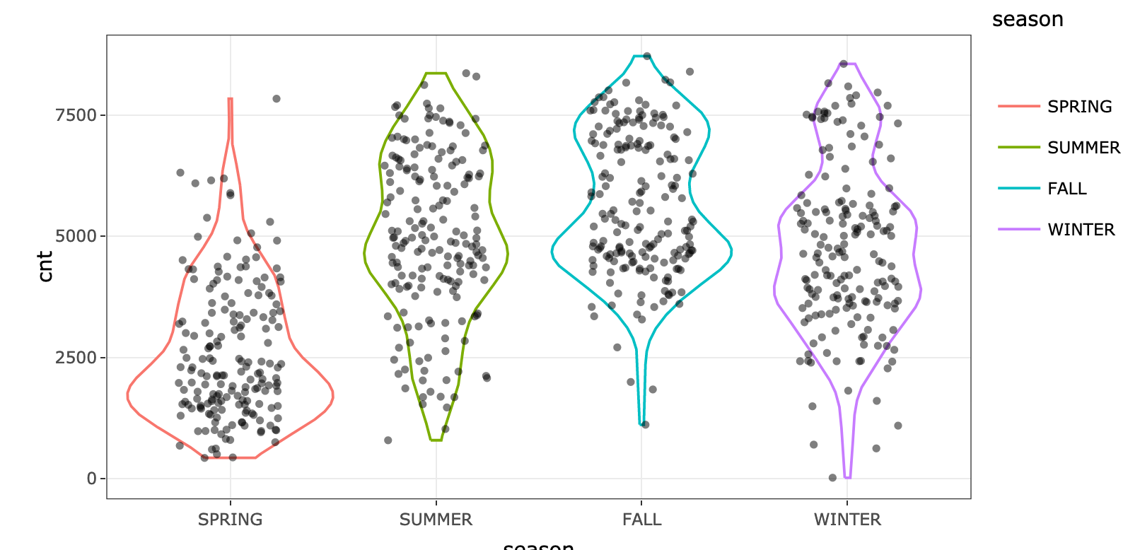 79 |
80 | As expected, rainy, snowy or stormy days are associated with less renting. However, if the value is `0`, it doesn't affect much the bike renting. Look at the yellow points around the 0 value. We can check the original variable and see the difference:
81 |
82 |
79 |
80 | As expected, rainy, snowy or stormy days are associated with less renting. However, if the value is `0`, it doesn't affect much the bike renting. Look at the yellow points around the 0 value. We can check the original variable and see the difference:
81 |
82 | 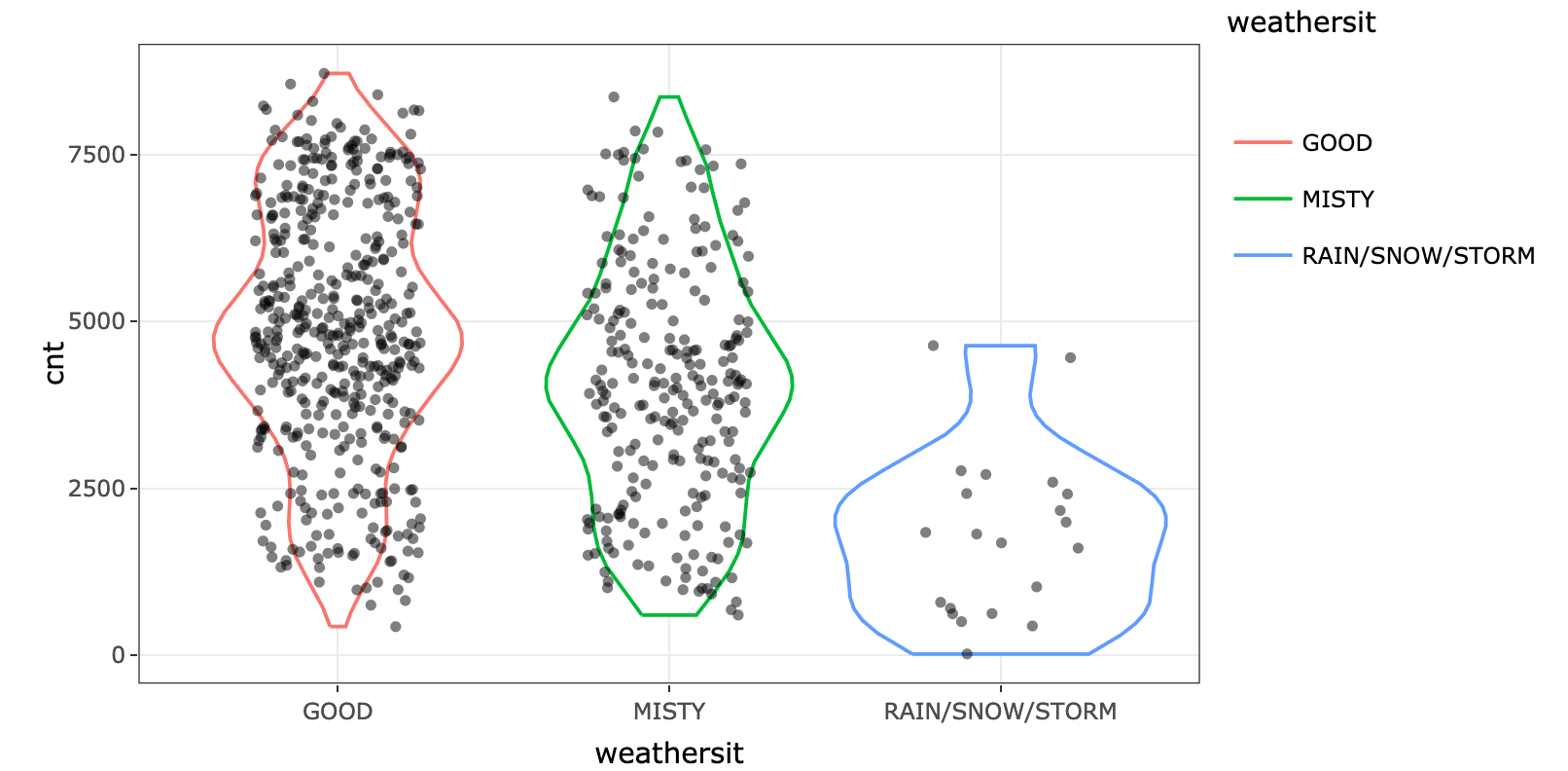 83 |
84 | What conclusion can you draw by looking at variables `weekday.SAT` and `weekday.MON`?
85 |
86 | ### Shap summary from xgboost package
87 |
88 | Function `xgb.plot.shap` from xgboost package provides these plots:
89 |
90 |
91 |
92 | * y-axis: shap value.
93 | * x-axis: original variable value.
94 |
95 | Each blue dot is a row (a _day_ in this case).
96 |
97 | Looking at `temp` variable, we can see how lower temperatures are associated with a big decrease in shap values. Interesting to note that around the value 22-23 the curve starts to decrease again. A perfect non-linear relationship.
98 |
99 | Taking `mnth.SEP` we can observe that dispersion around 0 is almost 0, while on the other hand, the value 1 is associated mainly with a shap increase around 200, but it also has certain days where it can push the shap value to more than 400.
100 |
101 | `mnth.SEP` is a good case of **interaction** with other variables, since in presence of the same value (`1`), the shap value can differ a lot. What are the effects with other variables that explain this variance in the output? A topic for another post.
102 |
103 |
104 | ## R packages with SHAP
105 |
106 | **[Interpretable Machine Learning](https://cran.r-project.org/web/packages/iml/vignettes/intro.html)** by Christoph Molnar.
107 |
108 |
83 |
84 | What conclusion can you draw by looking at variables `weekday.SAT` and `weekday.MON`?
85 |
86 | ### Shap summary from xgboost package
87 |
88 | Function `xgb.plot.shap` from xgboost package provides these plots:
89 |
90 |
91 |
92 | * y-axis: shap value.
93 | * x-axis: original variable value.
94 |
95 | Each blue dot is a row (a _day_ in this case).
96 |
97 | Looking at `temp` variable, we can see how lower temperatures are associated with a big decrease in shap values. Interesting to note that around the value 22-23 the curve starts to decrease again. A perfect non-linear relationship.
98 |
99 | Taking `mnth.SEP` we can observe that dispersion around 0 is almost 0, while on the other hand, the value 1 is associated mainly with a shap increase around 200, but it also has certain days where it can push the shap value to more than 400.
100 |
101 | `mnth.SEP` is a good case of **interaction** with other variables, since in presence of the same value (`1`), the shap value can differ a lot. What are the effects with other variables that explain this variance in the output? A topic for another post.
102 |
103 |
104 | ## R packages with SHAP
105 |
106 | **[Interpretable Machine Learning](https://cran.r-project.org/web/packages/iml/vignettes/intro.html)** by Christoph Molnar.
107 |
108 | 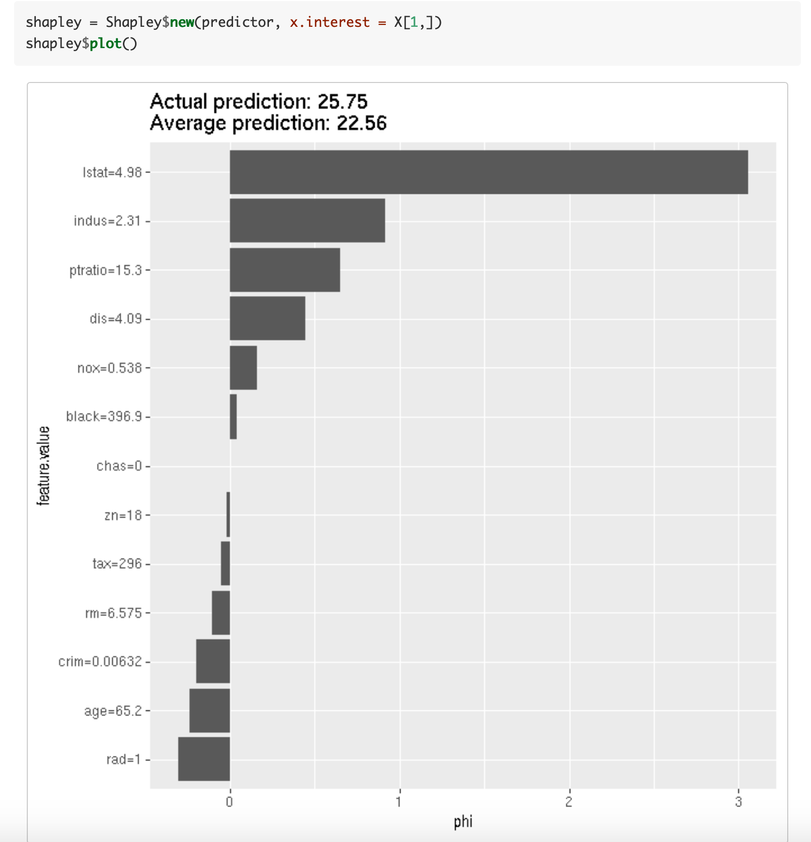 109 |
110 | **[xgboostExplainer](https://medium.com/applied-data-science/new-r-package-the-xgboost-explainer-51dd7d1aa211)**
111 |
112 | Altough it's not SHAP, the idea is really similar. It calculates the contribution for each value in every case, by accessing at the trees structure used in model.
113 |
114 |
109 |
110 | **[xgboostExplainer](https://medium.com/applied-data-science/new-r-package-the-xgboost-explainer-51dd7d1aa211)**
111 |
112 | Altough it's not SHAP, the idea is really similar. It calculates the contribution for each value in every case, by accessing at the trees structure used in model.
113 |
114 | 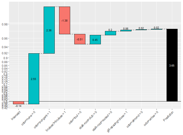 115 |
116 |
117 | ## Recommended literature about SHAP values `r emo::ji("books")`
118 |
119 | There is a vast literature around this technique, check the online book _Interpretable Machine Learning_ by Christoph Molnar. It addresses in a nicely way [Model-Agnostic Methods](https://christophm.github.io/interpretable-ml-book/agnostic.html) and one of its particular cases [Shapley values](https://christophm.github.io/interpretable-ml-book/shapley.html). An outstanding work.
120 |
121 | From classical variable, ranking approaches like _weight_ and _gain_, to shap values: [Interpretable Machine Learning with XGBoost](https://towardsdatascience.com/interpretable-machine-learning-with-xgboost-9ec80d148d27) by Scott Lundberg.
122 |
123 | A permutation perspective with examples: [One Feature Attribution Method to (Supposedly) Rule Them All: Shapley Values](https://towardsdatascience.com/one-feature-attribution-method-to-supposedly-rule-them-all-shapley-values-f3e04534983d).
124 |
125 |
126 | --
127 |
128 | Thanks for reading! `r emo::ji('rocket')`
129 |
130 |
131 | Other readings you might like:
132 |
133 | - [New discretization method: Recursive information gain ratio maximization](https://blog.datascienceheroes.com/discretization-recursive-gain-ratio-maximization/)
134 | - [Feature Selection using Genetic Algorithms in R](https://blog.datascienceheroes.com/feature-selection-using-genetic-algorithms-in-r/)
135 | - `r emo::ji('green_book')`[Data Science Live Book](http://livebook.datascienceheroes.com/)
136 |
137 | [Twitter](https://twitter.com/pabloc_ds) and [Linkedin](https://www.linkedin.com/in/pcasas/).
138 |
139 |
140 |
--------------------------------------------------------------------------------
/shap-values.Rproj:
--------------------------------------------------------------------------------
1 | Version: 1.0
2 |
3 | RestoreWorkspace: Default
4 | SaveWorkspace: Default
5 | AlwaysSaveHistory: Default
6 |
7 | EnableCodeIndexing: Yes
8 | UseSpacesForTab: Yes
9 | NumSpacesForTab: 2
10 | Encoding: UTF-8
11 |
12 | RnwWeave: Sweave
13 | LaTeX: pdfLaTeX
14 |
--------------------------------------------------------------------------------
/shap.R:
--------------------------------------------------------------------------------
1 | # Note: The functions shap.score.rank, shap_long_hd and plot.shap.summary were
2 | # originally published at https://liuyanguu.github.io/post/2018/10/14/shap-visualization-for-xgboost/
3 | # All the credits to the author.
4 |
5 |
6 | ## functions for plot
7 | # return matrix of shap score and mean ranked score list
8 | shap.score.rank <- function(xgb_model = xgb_mod, shap_approx = TRUE,
9 | X_train = mydata$train_mm){
10 | require(xgboost)
11 | require(data.table)
12 | shap_contrib <- predict(xgb_model, X_train,
13 | predcontrib = TRUE, approxcontrib = shap_approx)
14 | shap_contrib <- as.data.table(shap_contrib)
15 | shap_contrib[,BIAS:=NULL]
16 | cat('make SHAP score by decreasing order\n\n')
17 | mean_shap_score <- colMeans(abs(shap_contrib))[order(colMeans(abs(shap_contrib)), decreasing = T)]
18 | return(list(shap_score = shap_contrib,
19 | mean_shap_score = (mean_shap_score)))
20 | }
21 |
22 | # a function to standardize feature values into same range
23 | std1 <- function(x){
24 | return ((x - min(x, na.rm = T))/(max(x, na.rm = T) - min(x, na.rm = T)))
25 | }
26 |
27 |
28 | # prep shap data
29 | shap.prep <- function(shap = shap_result, X_train = mydata$train_mm, top_n){
30 | require(ggforce)
31 | # descending order
32 | if (missing(top_n)) top_n <- dim(X_train)[2] # by default, use all features
33 | if (!top_n%in%c(1:dim(X_train)[2])) stop('supply correct top_n')
34 | require(data.table)
35 | shap_score_sub <- as.data.table(shap$shap_score)
36 | shap_score_sub <- shap_score_sub[, names(shap$mean_shap_score)[1:top_n], with = F]
37 | shap_score_long <- melt.data.table(shap_score_sub, measure.vars = colnames(shap_score_sub))
38 |
39 | # feature values: the values in the original dataset
40 | fv_sub <- as.data.table(X_train)[, names(shap$mean_shap_score)[1:top_n], with = F]
41 | # standardize feature values
42 | fv_sub_long <- melt.data.table(fv_sub, measure.vars = colnames(fv_sub))
43 | fv_sub_long[, stdfvalue := std1(value), by = "variable"]
44 | # SHAP value: value
45 | # raw feature value: rfvalue;
46 | # standarized: stdfvalue
47 | names(fv_sub_long) <- c("variable", "rfvalue", "stdfvalue" )
48 | shap_long2 <- cbind(shap_score_long, fv_sub_long[,c('rfvalue','stdfvalue')])
49 | shap_long2[, mean_value := mean(abs(value)), by = variable]
50 | setkey(shap_long2, variable)
51 | return(shap_long2)
52 | }
53 |
54 | plot.shap.summary <- function(data_long){
55 | x_bound <- max(abs(data_long$value))
56 | require('ggforce') # for `geom_sina`
57 | plot1 <- ggplot(data = data_long)+
58 | coord_flip() +
59 | # sina plot:
60 | geom_sina(aes(x = variable, y = value, color = stdfvalue)) +
61 | # print the mean absolute value:
62 | geom_text(data = unique(data_long[, c("variable", "mean_value"), with = F]),
63 | aes(x = variable, y=-Inf, label = sprintf("%.3f", mean_value)),
64 | size = 3, alpha = 0.7,
65 | hjust = -0.2,
66 | fontface = "bold") + # bold
67 | # # add a "SHAP" bar notation
68 | # annotate("text", x = -Inf, y = -Inf, vjust = -0.2, hjust = 0, size = 3,
69 | # label = expression(group("|", bar(SHAP), "|"))) +
70 | scale_color_gradient(low="#FFCC33", high="#6600CC",
71 | breaks=c(0,1), labels=c("Low","High")) +
72 | theme_bw() +
73 | theme(axis.line.y = element_blank(), axis.ticks.y = element_blank(), # remove axis line
74 | legend.position="bottom") +
75 | geom_hline(yintercept = 0) + # the vertical line
76 | scale_y_continuous(limits = c(-x_bound, x_bound)) +
77 | # reverse the order of features
78 | scale_x_discrete(limits = rev(levels(data_long$variable))
79 | ) +
80 | labs(y = "SHAP value (impact on model output)", x = "", color = "Feature value")
81 | return(plot1)
82 | }
83 |
84 |
85 |
86 |
87 |
88 |
89 | var_importance <- function(shap_result, top_n=10)
90 | {
91 | var_importance=tibble(var=names(shap_result$mean_shap_score), importance=shap_result$mean_shap_score)
92 |
93 | var_importance=var_importance[1:top_n,]
94 |
95 | ggplot(var_importance, aes(x=reorder(var,importance), y=importance)) +
96 | geom_bar(stat = "identity") +
97 | coord_flip() +
98 | theme_light() +
99 | theme(axis.title.y=element_blank())
100 | }
101 |
--------------------------------------------------------------------------------
/shap_analysis.R:
--------------------------------------------------------------------------------
1 | library(tidyverse)
2 | library(xgboost)
3 | library(caret)
4 | source("shap.R")
5 |
6 | ##############################################
7 | # How to calculate and interpret shap values
8 | ##############################################
9 |
10 | load(url("https://github.com/christophM/interpretable-ml-book/blob/master/data/bike.RData?raw=true"))
11 | #readRDS("bike.RData")
12 |
13 | bike_2=select(bike, -days_since_2011, -cnt, -yr)
14 |
15 | bike_dmy = dummyVars(" ~ .", data = bike_2, fullRank=T)
16 | bike_x = predict(bike_dmy, newdata = bike_2)
17 |
18 | ## Create the xgboost model
19 | model_bike = xgboost(data = bike_x,
20 | nround = 10,
21 | objective="reg:linear",
22 | label= bike$cnt)
23 |
24 |
25 | cat("Note: The functions `shap.score.rank, `shap_long_hd` and `plot.shap.summary` were
26 | originally published at https://github.com/liuyanguu/Blogdown/blob/master/hugo-xmag/content/post/2018-10-05-shap-visualization-for-xgboost.Rmd
27 | All the credits to the author.")
28 |
29 | ## Calculate shap values
30 | shap_result_bike = shap.score.rank(xgb_model = model_bike,
31 | X_train =bike_x,
32 | shap_approx = F
33 | )
34 |
35 | # `shap_approx` comes from `approxcontrib` from xgboost documentation.
36 | # Faster but less accurate if true. Read more: help(xgboost)
37 |
38 | ## Plot var importance based on SHAP
39 | var_importance(shap_result_bike, top_n=10)
40 |
41 | ## Prepare data for top N variables
42 | shap_long_bike = shap.prep(shap = shap_result_bike,
43 | X_train = bike_x ,
44 | top_n = 10
45 | )
46 |
47 | ## Plot shap overall metrics
48 | plot.shap.summary(data_long = shap_long_bike)
49 |
50 |
51 | ##
52 | xgb.plot.shap(data = bike_x, # input data
53 | model = model_bike, # xgboost model
54 | features = names(shap_result_bike$mean_shap_score[1:10]), # only top 10 var
55 | n_col = 3, # layout option
56 | plot_loess = T # add red line to plot
57 | )
58 |
59 |
60 | # Do some classical plots
61 | # ggplotgui::ggplot_shiny(bike)
62 |
--------------------------------------------------------------------------------
/shap_heart_disease.R:
--------------------------------------------------------------------------------
1 | library(tidyverse)
2 | library(funModeling)
3 | library(xgboost)
4 | library(caret)
5 | source("shap.R")
6 |
7 | ## Some data preparation
8 | heart_disease_2=select(heart_disease, -has_heart_disease, -heart_disease_severity)
9 |
10 | dmytr = dummyVars(" ~ .", data = heart_disease_2, fullRank=T)
11 | heart_disease_3 = predict(dmytr, newdata = heart_disease_2)
12 | target_var=ifelse(as.character(heart_disease$has_heart_disease)=="yes", 1,0)
13 |
14 | ## Create the xgboost model
15 | model_hd = xgboost(data = heart_disease_3,
16 | nround = 10,
17 | objective = "binary:logistic",
18 | label= target_var)
19 |
20 | ## Calculate shap values
21 | shap_result = shap.score.rank(xgb_model = model_hd,
22 | X_train = heart_disease_3,
23 | shap_approx = F)
24 |
25 | ## Plot var importance
26 | var_importance(shap_result, top_n=10)
27 |
28 | ## Prepare shap data
29 | shap_long_hd = shap.prep(X_train = heart_disease_3 , top_n = 10)
30 |
31 | ## Plot shap overall metrics
32 | plot.shap.summary(data_long = shap_long_hd)
33 |
34 | # Note: The functions shap.score.rank, shap_long_hd and plot.shap.summary were
35 | # originally published at https://liuyanguu.github.io/post/2018/10/14/shap-visualization-for-xgboost/
36 | # All the credits to the author.
37 |
38 |
39 | ## Shap
40 | xgb.plot.shap(data = heart_disease_3,
41 | model = model_hd,
42 | features = names(shap_result$mean_shap_score)[1:10],
43 | n_col = 3,
44 | plot_loess = T)
45 |
46 |
47 | ################################
48 | # Dowload the file from here:
49 | # https://github.com/christophM/interpretable-ml-book/blob/master/data/bike.RData
50 | load("bike.RData")
51 | bike_2=select(bike, -days_since_2011, -cnt, -yr)
52 |
53 | bike_dmy = dummyVars(" ~ .", data = bike_2, fullRank=T)
54 | bike_x = predict(bike_dmy, newdata = bike_2)
55 |
56 |
57 | ## Create the xgboost model
58 | model_bike = xgboost(data = bike_x,
59 | nround = 10,
60 | objective="reg:linear",
61 | label= bike$cnt)
62 |
63 |
64 |
65 | ## Calculate shap values
66 | shap_result_bike = shap.score.rank(xgb_model = model_bike,
67 | X_train =bike_x,
68 | shap_approx = F
69 | )
70 |
71 |
72 | # `shap_approx` comes from `approxcontrib ` from xgboost documentation.
73 | # Faster but less accurate if true. Read more: help(xgboost)
74 |
75 |
76 | ## Plot var importance
77 | var_importance(shap_result_bike, top_n=10)
78 |
79 | ## Prepare shap data
80 | shap_long_bike = shap.prep(X_train = bike_x , top_n = 10)
81 |
82 | ## Plot shap overall metrics
83 | plot.shap.summary(data_long = shap_long_bike)
84 |
85 |
86 | ##
87 | xgb.plot.shap(data = bike_x,
88 | model = model_bike,
89 | features = names(shap_result_bike$mean_shap_score[1:10]),
90 | n_col = 3, plot_loess = T)
91 |
92 |
93 |
94 | ggplotgui::ggplot_shiny(bike)
95 |
--------------------------------------------------------------------------------
115 |
116 |
117 | ## Recommended literature about SHAP values `r emo::ji("books")`
118 |
119 | There is a vast literature around this technique, check the online book _Interpretable Machine Learning_ by Christoph Molnar. It addresses in a nicely way [Model-Agnostic Methods](https://christophm.github.io/interpretable-ml-book/agnostic.html) and one of its particular cases [Shapley values](https://christophm.github.io/interpretable-ml-book/shapley.html). An outstanding work.
120 |
121 | From classical variable, ranking approaches like _weight_ and _gain_, to shap values: [Interpretable Machine Learning with XGBoost](https://towardsdatascience.com/interpretable-machine-learning-with-xgboost-9ec80d148d27) by Scott Lundberg.
122 |
123 | A permutation perspective with examples: [One Feature Attribution Method to (Supposedly) Rule Them All: Shapley Values](https://towardsdatascience.com/one-feature-attribution-method-to-supposedly-rule-them-all-shapley-values-f3e04534983d).
124 |
125 |
126 | --
127 |
128 | Thanks for reading! `r emo::ji('rocket')`
129 |
130 |
131 | Other readings you might like:
132 |
133 | - [New discretization method: Recursive information gain ratio maximization](https://blog.datascienceheroes.com/discretization-recursive-gain-ratio-maximization/)
134 | - [Feature Selection using Genetic Algorithms in R](https://blog.datascienceheroes.com/feature-selection-using-genetic-algorithms-in-r/)
135 | - `r emo::ji('green_book')`[Data Science Live Book](http://livebook.datascienceheroes.com/)
136 |
137 | [Twitter](https://twitter.com/pabloc_ds) and [Linkedin](https://www.linkedin.com/in/pcasas/).
138 |
139 |
140 |
--------------------------------------------------------------------------------
/shap-values.Rproj:
--------------------------------------------------------------------------------
1 | Version: 1.0
2 |
3 | RestoreWorkspace: Default
4 | SaveWorkspace: Default
5 | AlwaysSaveHistory: Default
6 |
7 | EnableCodeIndexing: Yes
8 | UseSpacesForTab: Yes
9 | NumSpacesForTab: 2
10 | Encoding: UTF-8
11 |
12 | RnwWeave: Sweave
13 | LaTeX: pdfLaTeX
14 |
--------------------------------------------------------------------------------
/shap.R:
--------------------------------------------------------------------------------
1 | # Note: The functions shap.score.rank, shap_long_hd and plot.shap.summary were
2 | # originally published at https://liuyanguu.github.io/post/2018/10/14/shap-visualization-for-xgboost/
3 | # All the credits to the author.
4 |
5 |
6 | ## functions for plot
7 | # return matrix of shap score and mean ranked score list
8 | shap.score.rank <- function(xgb_model = xgb_mod, shap_approx = TRUE,
9 | X_train = mydata$train_mm){
10 | require(xgboost)
11 | require(data.table)
12 | shap_contrib <- predict(xgb_model, X_train,
13 | predcontrib = TRUE, approxcontrib = shap_approx)
14 | shap_contrib <- as.data.table(shap_contrib)
15 | shap_contrib[,BIAS:=NULL]
16 | cat('make SHAP score by decreasing order\n\n')
17 | mean_shap_score <- colMeans(abs(shap_contrib))[order(colMeans(abs(shap_contrib)), decreasing = T)]
18 | return(list(shap_score = shap_contrib,
19 | mean_shap_score = (mean_shap_score)))
20 | }
21 |
22 | # a function to standardize feature values into same range
23 | std1 <- function(x){
24 | return ((x - min(x, na.rm = T))/(max(x, na.rm = T) - min(x, na.rm = T)))
25 | }
26 |
27 |
28 | # prep shap data
29 | shap.prep <- function(shap = shap_result, X_train = mydata$train_mm, top_n){
30 | require(ggforce)
31 | # descending order
32 | if (missing(top_n)) top_n <- dim(X_train)[2] # by default, use all features
33 | if (!top_n%in%c(1:dim(X_train)[2])) stop('supply correct top_n')
34 | require(data.table)
35 | shap_score_sub <- as.data.table(shap$shap_score)
36 | shap_score_sub <- shap_score_sub[, names(shap$mean_shap_score)[1:top_n], with = F]
37 | shap_score_long <- melt.data.table(shap_score_sub, measure.vars = colnames(shap_score_sub))
38 |
39 | # feature values: the values in the original dataset
40 | fv_sub <- as.data.table(X_train)[, names(shap$mean_shap_score)[1:top_n], with = F]
41 | # standardize feature values
42 | fv_sub_long <- melt.data.table(fv_sub, measure.vars = colnames(fv_sub))
43 | fv_sub_long[, stdfvalue := std1(value), by = "variable"]
44 | # SHAP value: value
45 | # raw feature value: rfvalue;
46 | # standarized: stdfvalue
47 | names(fv_sub_long) <- c("variable", "rfvalue", "stdfvalue" )
48 | shap_long2 <- cbind(shap_score_long, fv_sub_long[,c('rfvalue','stdfvalue')])
49 | shap_long2[, mean_value := mean(abs(value)), by = variable]
50 | setkey(shap_long2, variable)
51 | return(shap_long2)
52 | }
53 |
54 | plot.shap.summary <- function(data_long){
55 | x_bound <- max(abs(data_long$value))
56 | require('ggforce') # for `geom_sina`
57 | plot1 <- ggplot(data = data_long)+
58 | coord_flip() +
59 | # sina plot:
60 | geom_sina(aes(x = variable, y = value, color = stdfvalue)) +
61 | # print the mean absolute value:
62 | geom_text(data = unique(data_long[, c("variable", "mean_value"), with = F]),
63 | aes(x = variable, y=-Inf, label = sprintf("%.3f", mean_value)),
64 | size = 3, alpha = 0.7,
65 | hjust = -0.2,
66 | fontface = "bold") + # bold
67 | # # add a "SHAP" bar notation
68 | # annotate("text", x = -Inf, y = -Inf, vjust = -0.2, hjust = 0, size = 3,
69 | # label = expression(group("|", bar(SHAP), "|"))) +
70 | scale_color_gradient(low="#FFCC33", high="#6600CC",
71 | breaks=c(0,1), labels=c("Low","High")) +
72 | theme_bw() +
73 | theme(axis.line.y = element_blank(), axis.ticks.y = element_blank(), # remove axis line
74 | legend.position="bottom") +
75 | geom_hline(yintercept = 0) + # the vertical line
76 | scale_y_continuous(limits = c(-x_bound, x_bound)) +
77 | # reverse the order of features
78 | scale_x_discrete(limits = rev(levels(data_long$variable))
79 | ) +
80 | labs(y = "SHAP value (impact on model output)", x = "", color = "Feature value")
81 | return(plot1)
82 | }
83 |
84 |
85 |
86 |
87 |
88 |
89 | var_importance <- function(shap_result, top_n=10)
90 | {
91 | var_importance=tibble(var=names(shap_result$mean_shap_score), importance=shap_result$mean_shap_score)
92 |
93 | var_importance=var_importance[1:top_n,]
94 |
95 | ggplot(var_importance, aes(x=reorder(var,importance), y=importance)) +
96 | geom_bar(stat = "identity") +
97 | coord_flip() +
98 | theme_light() +
99 | theme(axis.title.y=element_blank())
100 | }
101 |
--------------------------------------------------------------------------------
/shap_analysis.R:
--------------------------------------------------------------------------------
1 | library(tidyverse)
2 | library(xgboost)
3 | library(caret)
4 | source("shap.R")
5 |
6 | ##############################################
7 | # How to calculate and interpret shap values
8 | ##############################################
9 |
10 | load(url("https://github.com/christophM/interpretable-ml-book/blob/master/data/bike.RData?raw=true"))
11 | #readRDS("bike.RData")
12 |
13 | bike_2=select(bike, -days_since_2011, -cnt, -yr)
14 |
15 | bike_dmy = dummyVars(" ~ .", data = bike_2, fullRank=T)
16 | bike_x = predict(bike_dmy, newdata = bike_2)
17 |
18 | ## Create the xgboost model
19 | model_bike = xgboost(data = bike_x,
20 | nround = 10,
21 | objective="reg:linear",
22 | label= bike$cnt)
23 |
24 |
25 | cat("Note: The functions `shap.score.rank, `shap_long_hd` and `plot.shap.summary` were
26 | originally published at https://github.com/liuyanguu/Blogdown/blob/master/hugo-xmag/content/post/2018-10-05-shap-visualization-for-xgboost.Rmd
27 | All the credits to the author.")
28 |
29 | ## Calculate shap values
30 | shap_result_bike = shap.score.rank(xgb_model = model_bike,
31 | X_train =bike_x,
32 | shap_approx = F
33 | )
34 |
35 | # `shap_approx` comes from `approxcontrib` from xgboost documentation.
36 | # Faster but less accurate if true. Read more: help(xgboost)
37 |
38 | ## Plot var importance based on SHAP
39 | var_importance(shap_result_bike, top_n=10)
40 |
41 | ## Prepare data for top N variables
42 | shap_long_bike = shap.prep(shap = shap_result_bike,
43 | X_train = bike_x ,
44 | top_n = 10
45 | )
46 |
47 | ## Plot shap overall metrics
48 | plot.shap.summary(data_long = shap_long_bike)
49 |
50 |
51 | ##
52 | xgb.plot.shap(data = bike_x, # input data
53 | model = model_bike, # xgboost model
54 | features = names(shap_result_bike$mean_shap_score[1:10]), # only top 10 var
55 | n_col = 3, # layout option
56 | plot_loess = T # add red line to plot
57 | )
58 |
59 |
60 | # Do some classical plots
61 | # ggplotgui::ggplot_shiny(bike)
62 |
--------------------------------------------------------------------------------
/shap_heart_disease.R:
--------------------------------------------------------------------------------
1 | library(tidyverse)
2 | library(funModeling)
3 | library(xgboost)
4 | library(caret)
5 | source("shap.R")
6 |
7 | ## Some data preparation
8 | heart_disease_2=select(heart_disease, -has_heart_disease, -heart_disease_severity)
9 |
10 | dmytr = dummyVars(" ~ .", data = heart_disease_2, fullRank=T)
11 | heart_disease_3 = predict(dmytr, newdata = heart_disease_2)
12 | target_var=ifelse(as.character(heart_disease$has_heart_disease)=="yes", 1,0)
13 |
14 | ## Create the xgboost model
15 | model_hd = xgboost(data = heart_disease_3,
16 | nround = 10,
17 | objective = "binary:logistic",
18 | label= target_var)
19 |
20 | ## Calculate shap values
21 | shap_result = shap.score.rank(xgb_model = model_hd,
22 | X_train = heart_disease_3,
23 | shap_approx = F)
24 |
25 | ## Plot var importance
26 | var_importance(shap_result, top_n=10)
27 |
28 | ## Prepare shap data
29 | shap_long_hd = shap.prep(X_train = heart_disease_3 , top_n = 10)
30 |
31 | ## Plot shap overall metrics
32 | plot.shap.summary(data_long = shap_long_hd)
33 |
34 | # Note: The functions shap.score.rank, shap_long_hd and plot.shap.summary were
35 | # originally published at https://liuyanguu.github.io/post/2018/10/14/shap-visualization-for-xgboost/
36 | # All the credits to the author.
37 |
38 |
39 | ## Shap
40 | xgb.plot.shap(data = heart_disease_3,
41 | model = model_hd,
42 | features = names(shap_result$mean_shap_score)[1:10],
43 | n_col = 3,
44 | plot_loess = T)
45 |
46 |
47 | ################################
48 | # Dowload the file from here:
49 | # https://github.com/christophM/interpretable-ml-book/blob/master/data/bike.RData
50 | load("bike.RData")
51 | bike_2=select(bike, -days_since_2011, -cnt, -yr)
52 |
53 | bike_dmy = dummyVars(" ~ .", data = bike_2, fullRank=T)
54 | bike_x = predict(bike_dmy, newdata = bike_2)
55 |
56 |
57 | ## Create the xgboost model
58 | model_bike = xgboost(data = bike_x,
59 | nround = 10,
60 | objective="reg:linear",
61 | label= bike$cnt)
62 |
63 |
64 |
65 | ## Calculate shap values
66 | shap_result_bike = shap.score.rank(xgb_model = model_bike,
67 | X_train =bike_x,
68 | shap_approx = F
69 | )
70 |
71 |
72 | # `shap_approx` comes from `approxcontrib ` from xgboost documentation.
73 | # Faster but less accurate if true. Read more: help(xgboost)
74 |
75 |
76 | ## Plot var importance
77 | var_importance(shap_result_bike, top_n=10)
78 |
79 | ## Prepare shap data
80 | shap_long_bike = shap.prep(X_train = bike_x , top_n = 10)
81 |
82 | ## Plot shap overall metrics
83 | plot.shap.summary(data_long = shap_long_bike)
84 |
85 |
86 | ##
87 | xgb.plot.shap(data = bike_x,
88 | model = model_bike,
89 | features = names(shap_result_bike$mean_shap_score[1:10]),
90 | n_col = 3, plot_loess = T)
91 |
92 |
93 |
94 | ggplotgui::ggplot_shiny(bike)
95 |
--------------------------------------------------------------------------------