 19 |
19 |
18 |
19 |
39 |  40 |
40 |
46 |  47 |
47 |  48 |
48 |
 56 |
57 | ## Configuration
58 |
59 | The argument `#averageLinkage` in the code above is used to compute the distance of new clusters to the other ones.
60 | There are 3 values possible:
61 | - `#singleLinkage`: Distance between two clusters is the distance between their two closest (more similar) objects.
62 | - `#averageLinkage`: Distance between two clusters is the arithmetic mean of all the distances between the objects of one and the objects of the other.
63 | - `#completeLinkage`: Distance between two clusters is the distance between their two most dissimilar objects.
64 |
65 | Single Linkage can result in clusters formed of a "chain of elements" but the first and last elements quite far from one another.
66 |
67 |
56 |
57 | ## Configuration
58 |
59 | The argument `#averageLinkage` in the code above is used to compute the distance of new clusters to the other ones.
60 | There are 3 values possible:
61 | - `#singleLinkage`: Distance between two clusters is the distance between their two closest (more similar) objects.
62 | - `#averageLinkage`: Distance between two clusters is the arithmetic mean of all the distances between the objects of one and the objects of the other.
63 | - `#completeLinkage`: Distance between two clusters is the distance between their two most dissimilar objects.
64 |
65 | Single Linkage can result in clusters formed of a "chain of elements" but the first and last elements quite far from one another.
66 |
67 |  68 |
69 | Complete linkage results in clusters with "compact contours", but elements not necessarily compact inside.
70 | Notice that the left branch of the big cluster (ie. top branch on the plot) is better balanced with Complete linkage than with Average linkage (first figure above)
71 |
72 |
68 |
69 | Complete linkage results in clusters with "compact contours", but elements not necessarily compact inside.
70 | Notice that the left branch of the big cluster (ie. top branch on the plot) is better balanced with Complete linkage than with Average linkage (first figure above)
71 |
72 |  73 |
74 | ## Distance matrix
75 |
76 | In the code above, the distance matrix is a default one computed from the elements.
77 | In this case the distance is the sum of the square differences between two vectors.
78 |
79 | One can provide a different matrix using any other possible metrics.
80 | This must be a **distance** matrix (higher value means more different), not a similarity matrix (higher value mean more similar).
81 |
82 | ## Threshold
83 |
84 | In the plots, the horizontal bar are not always at the same position.
85 | This depends on the `threshold` of each cluster.
86 | The threshold of a cluster can be seen as the distance between its two elements.
87 |
88 | With less elements, the threshold is typically small (elements close one to the other).
89 | With more elements, the difference start to be bigger and the threshold augment.
90 |
91 | If you compare the first plot (average linkage) and the last one (complete linkage), you might see that the threshold of the first left node is smaller with average linkage.
92 | The two clusters contain the same elements (10 elements with a 0 as second part).
93 | But because complete linkage computes the distance between two clusters as the distance between their two most dissimilar objects, the threshold ends up being higher.
--------------------------------------------------------------------------------
/wiki/Tutorials/market-basket-analysis-using-a-priori.md:
--------------------------------------------------------------------------------
1 | # Market Basket Analysis using A-Priori Algorithm
2 |
3 | In this tutorial we will show an application of the A-Priori algorithm.
4 | You can find it at [pharo-ai/a-priori](https://github.com/pharo-ai/APriori).
5 | We will analyze a dataset that contains a list of transactions of supermarket items that were bought.
6 |
7 | You need to install the A-Priori algorithm.
8 | To do that, execute the following script in your Pharo image:
9 |
10 | ```st
11 | Metacello new
12 | repository: 'github://pharo-ai/a-priori:v1.0.0';
13 | baseline: 'AIAPriori';
14 | load.
15 | ```
16 |
17 | The A-Priori algorithm is going to give us some associations rule of the most frequently items that are bought together.
18 | For example, if someone goes to the supermarket and buys eggs, butter vegetables and yogurt is likely that they will buy milk too.
19 |
20 | ## Importing the data
21 |
22 | First, let's download the [dataset CSV file from Kaggle](https://www.kaggle.com/datasets/irfanasrullah/groceries).
23 |
24 | Then, we need to import the csv file into memory with this line. You need to change the path to location of where you downloaded the file.
25 |
26 | ```st
27 | file := 'your-path-to-the-file/groceries.csv' asFileReference.
28 | ```
29 |
30 | If we inspect the contents of the file, we will see that we have some empty spaces. Also it has a header.
31 |
32 | 
33 |
34 | So, we will do a little pre-processing to clean this dataset. We will divide each line by commas and then we will reject the empty fields.
35 |
36 | ```st
37 | transactions := file contents lines allButFirst collect: [ :line |
38 | (',' split: line) allButFirst reject: [ :item | item isEmpty ] ].
39 | ```
40 |
41 | ## Instantiating A-Priori Algorithm
42 |
43 | We need to create an instance of `APrioriTransactionsArray`.
44 | It is only an object in which we need to pass the array of `transactions`.
45 |
46 | ```st
47 | transactionsSource := APrioriTransactionsArray from: transactions.
48 | ```
49 |
50 | Then, we instantiate the A-Priori algorithm with the transactions object that we just created.
51 |
52 | ```st
53 | apriori := APriori forTransactions: transactionsSource.
54 | ```
55 |
56 | A-Priori will find the combinations of items (we call them itemsets) that frequently appear together.
57 | To do that, first we need to define, what it means to be "frequent".
58 | This can be expressed with a metric called _support_ -- a percentage of transactions in which the given itemset appears.
59 | By setting a minimum support threshold of 1\%, we tell the A-Priori algorithm that it should only select the combinations of items that appear in at least 1% of transactions.
60 |
61 | ```st
62 | apriori minSupport: 0.01.
63 | ```
64 |
65 | For running the algorithm we need to send the message `findFrequentItemsets` to the a-priori object.
66 |
67 | ```st
68 | apriori findFrequentItemsets.
69 | ```
70 |
71 | The `apriori` object will mine frequent itemsets from the dataset of transactions and store them in `apriori frequentItemsets` attribute.
72 | Those will include itemsets that only contain one item (for example, 50% of customers buy water, which means that water is a frequently purchased item).
73 | But in our case, we are only interested in co-occurences of items (pairs, triplets, etc.) so we remove all frequent itemsets of size 1:
74 |
75 | ```st
76 | frequentItemsets := apriori frequentItemsets select: [ :each | each size > 1 ].
77 | ```
78 |
79 | Now we can ask A-Priori to build the association rules with `buildAssociationRules`.
80 | Those are the rules in form `{left itemset} -> {right itemset}` that represent the situation when client has already purchased the items on the left and now we want to recommend him or her the items on the right.
81 |
82 | ```st
83 | apriori buildAssociationRules.
84 | ```
85 |
86 | We built *all* the associations of the transactions. That means that we built all the combinations of the items that were bought together. Now we need to filter them.
87 | Because we only want to get the rules which have high _confidence_.
88 | Confidence is another metric which tells us the conditional probability of a cient purchasing the items on the right given that this same client has already purchased items on the left.
89 | We ask A-Priori to calculate confidence:
90 |
91 | ```st
92 | apriori calculateAssociationRuleMetrics: {
93 | APrioriConfidenceMetric }.
94 | ```
95 |
96 | Now we can filter the association rules that have at least 50\% confidence:
97 |
98 | ```st
99 | rules := apriori associationRules select: [ :each | each confidence >= 0.5 ].
100 | ```
101 |
102 | ## Summary of the code
103 |
104 | ```st
105 | file := 'your-path-to-the-file/groceries.csv' asFileReference.
106 |
107 | transactions := file contents lines allButFirst collect: [ :line |
108 | (',' split: line) allButFirst reject: [ :item | item isEmpty ] ].
109 |
110 | transactionsSource := APrioriTransactionsArray from: transactions.
111 |
112 | apriori := APriori forTransactions: transactionsSource.
113 |
114 | apriori minSupport: 0.01.
115 |
116 | apriori findFrequentItemsets.
117 |
118 | frequentItemsets := apriori frequentItemsets select: [ :each | each size > 1 ].
119 |
120 | apriori buildAssociationRules.
121 |
122 | apriori calculateAssociationRuleMetrics: {
123 | APrioriConfidenceMetric .
124 | APrioriLiftMetric }.
125 |
126 | rules := apriori associationRules select: [ :each | each confidence >= 0.5 ].
127 | ```
128 |
--------------------------------------------------------------------------------
/wiki/MachineLearning/Linear-Regression.md:
--------------------------------------------------------------------------------
1 | # Linear regression
2 |
3 | Repository: https://github.com/pharo-ai/linear-models
4 |
5 | ## Table of contents
6 |
7 | - [Linear Regression with Gradient Descent](#linear-regression-with-gradient-descent)
8 | - [Measuring the accuracy of a model](#measuring-the-accuracy-of-a-model)
9 | - [Linear Regression with Least Squares using Pharo-Lapack](#linear-regression-with-least-squares-using-pharo-lapack)
10 | - [Linear Regression with Least Squares using PolyMath](#linear-regression-with-least-squares-using-polymath)
11 |
12 | ## Linear Regression with Gradient Descent
13 | Linear regression is a well-known machine learning algorithms.
14 | It allows us to learn the linear dependency between the input variables $x_1, \dots, x_n$ and the output variable $y$.
15 | Attempts to find the the linear relationship between one or more input variables _x1, x2, ..., xn_ and an output variable _y_. It finds a set of parameters _b, w1, w2, ..., wn_ such that the predicted output _h(x) = b + w1 * x1 + ... + wn * xn_ is as close as possible to the real output _y_. Then we can use the trained model to predict the previously unseen values of y.
16 |
17 | For example:
18 |
19 | Given 20 input vectors _x = (x1, x2, x3)_ and 20 output values _y_.
20 |
21 | ```Smalltalk
22 | input := #( (-6 0.44 3) (4 -0.45 -7) (-4 -0.16 4) (9 0.17 -8) (-6 -0.41 8)
23 | (9 0.03 6) (-2 -0.26 -4) (-3 -0.02 -6) (6 -0.18 -2) (-6 -0.11 9)
24 | (-10 0.15 -8) (-8 -0.13 7) (3 -0.29 1) (8 -0.21 -1) (-3 0.12 7)
25 | (4 0.03 5) (3 -0.27 2) (-8 -0.21 -10) (-10 -0.41 -8) (-5 0.11 0)).
26 |
27 | output := #(-10.6 10.5 -13.6 27.7 -24.1 12.3 -2.6 -0.2 12.2 -22.1 -10.5 -24.3 2.1 14.9 -11.8 3.3 1.3 -8.1 -16.1 -8.9).
28 | ```
29 |
30 | We want to find the linear relationships between the input and the output. In other words, we need to find such parameters _b, w1, w2, w3_ that the line _h(x) = b + w1 * x1 + w2 * x2 + w3 * x3_ fits the data as closely as possible. To do that, we initialize a linear regression model and fit it to the data.
31 |
32 | ```Smalltalk
33 | linearRegressionModel := AILinearRegression new
34 | learningRate: 0.001;
35 | maxIterations: 2000;
36 | yourself.
37 |
38 | linearRegressionModel fitX: input y: output.
39 | ```
40 |
41 | Now we can look at the trained parameters. The real relationship between x and y is _y = 2*x1 + 10*x2 - x3_, so the parameters should be close to _b=0_, _w1=2_, _w2=10_, _w3=-1_.
42 |
43 | ```Smalltalk
44 | b := linearRegressionModel bias.
45 | "-0.0029744215186773065"
46 | w := linearRegressionModel weights.
47 | "#(1.9999658061022905 9.972821149946537 -0.9998757756318858)"
48 | ```
49 |
50 | Finally, we can use the model to predict the output of previously unseen input.
51 |
52 | ```Smalltalk
53 | testInput := #( (-3 0.43 1) (-3 -0.11 -7)
54 | (-6 0.06 -9) (-7 -0.41 7) (3 0.43 10)).
55 |
56 | expectedOutput := #(-2.7 -0.01 -2.4 -25.1 0.3).
57 | ```
58 |
59 | ```Smalltalk
60 | linearRegressionModel predict: testInput.
61 | "#(-2.7144345209804244 -0.10075173689646852 -2.405518008448657 -25.090722165135997 0.28647833494634645)"
62 | ```
63 |
64 | ## Measuring the accuracy of a model
65 |
66 | Please refer to the wiki for [Measuring the accuracy of a model](./Measuring-the-accuracy-of-a-model.md)
67 |
68 | ## Linear Regression with Least Squares using Pharo-Lapack
69 |
70 | We have implemented the class `AILinearRegressionLeastSquares` that also trains a linear regression model but using other approach. The class `AILinearRegression` uses the gradient descent algorithm for finding the weights of the model. With the class `AILinearRegressionLeastSquares` we model the problems in terms of the least squares problem and we solve it using [Linear Algebra](../LinearAlgebra/Lapack.md). It's a package for solving linear algebra problem, like least squares.That library uses [Pharo-Lapack](../LinearAlgebra/Lapack.md), that is a binding for Lapack in Pharo. We use Lapack for speed up the computation, as Lapack it's a highly optimized library written in Fortran.
71 |
72 | The prerequisite is that you need to have Lapack installed on your computer. If you use a Mac, you have it already installed by default. You can check [this link](https://netlib.org/lapack/lug/node14.html) for installing it.
73 |
74 | ### How to use it
75 |
76 | This class has the same API for training and predicting as the other ones.
77 |
78 | ```st
79 | linearRegressionModel := AILinearRegressionLeastSquares new.
80 |
81 | linearRegressionModel fitX: input y: output.
82 | linearRegressionModel predict: testInput.
83 | ```
84 |
85 | The difference is that you need to use the class `AIColumnMajorMatrix` or even `AINativeFloatMatrix`. Those are matrices data structures that we implemented meant to be used with Lapack. They are optimized to avoid transposing the matrix and copying the data.
86 |
87 | You can create the matrices using the class side message `rows`
88 |
89 |
90 | ```st
91 | AIColumnMajorMatrix rows: (
92 | (12 3 5)
93 | (1 4 17)
94 | (3 7 33)
95 | ).
96 |
97 | AINativeFloatMatrix rows: (
98 | (12 3 5)
99 | (1 4 17)
100 | (3 7 33)
101 | ).
102 | ```
103 |
104 | For more information, please refer to the wiki pages [Linear Algebra](../LinearAlgebra/LinearAlgebra.md) and [Lapack](../LinearAlgebra/Lapack.md)
105 |
106 |
107 | ### Linear Regression with Least Squares using PolyMath
108 |
109 | We also have the class `AILinearRegressionLeastSquaresVanilla` that is a subclass of `AILinearRegressionLeastSquares`. But it uses PolyMath that is written in pure Pharo. You can call the fit method with an array of array, as it doesn't use Lapack, you don't need the special data structures.
110 |
--------------------------------------------------------------------------------
/wiki/DataExploration/Metrics.md:
--------------------------------------------------------------------------------
1 | # Metrics for Machine Learning
2 |
3 | Repository: https://github.com/pharo-ai/metrics
4 |
5 | In this packages we have implemented several metris for different machine learning algorithm types.
6 |
7 | _Note: This is currently work in progress. More metrics will be added in the future and maybe also changes in the architecture._
8 |
9 | ## Table of Contents
10 |
11 | - [Clustering metrics](#clustering-metrics)
12 | - [Regression metrics](#regression-metrics)
13 | - [Classification metrics](#classification-metrics)
14 |
15 | ## Clustering metrics
16 |
17 | - Jaccard Index (`AIJaccardIndex`)
18 | - Rand Index (`AIRandIndex`)
19 | - Silhouette Index (`AISilhouetteIndex`)
20 | - Adjusted Rand Index (`AIAdjustedRandIndex`)
21 | - Fowlkes Mallows Index (`AIFowlkesMallowsIndex`)
22 | - Mirkin Index (`AIMirkinIndex`)
23 | - Weighted Jaccard Index (`AIWeightedJaccardIndex`)
24 |
25 | ## Regression metrics
26 |
27 | - [Mean Squared Error](#mean-squared-error)
28 | - [Mean Absolute Error](#mean-absolute-error)
29 | - [Mean Squared Logarithmic Error](#mean-squared-logarithmic-error)
30 | - [R2 Score](#r2-score)
31 | - [Root Mean Squared Error](#root-mean-squared-error)
32 | - [Max Error](#max-error)
33 | - [Explained Variance Score](#explained-variance-score)
34 |
35 | This package also contains regression metrics for testing the performance of different machine learning models. For example: Logistic and Linear regression.
36 | Part of this text for the explanation were extracted from [scikit-learn documentation](https://scikit-learn.org/stable/modules/model_evaluation.html)
37 |
38 | ### Mean Squared Error
39 |
40 | The mean_squared_error function computes mean square error, a risk metric corresponding to the expected value of the squared (quadratic) error or loss.
41 |
42 | ```st
43 | | yActual yPredicted metric |
44 | metric := AIMeanSquaredError new.
45 | yActual := #( 3 -0.5 2 7 ).
46 | yPredicted := #( 2.5 0.0 2 8 ).
47 | metric computeForActual: yActual predicted: yPredicted "0.375"
48 | ```
49 |
50 | ### Mean Absolute Error
51 |
52 | The mean absolute error function computes mean absolute error, a risk metric corresponding to the expected value of the absolute error loss or -norm loss.
53 |
54 | ```st
55 | | yActual yPredicted metric |
56 | metric := AIMeanAbsoluteError new.
57 | yActual := #( 3 -0.5 2 7 ).
58 | yPredicted := #( 2.5 0.0 2 8 ).
59 | metric computeForActual: yActual predicted: yPredicted "0.5"
60 | ```
61 |
62 | ### Mean Squared Logarithmic Error
63 |
64 | The mean squared log error function computes a risk metric corresponding to the expected value of the squared logarithmic (quadratic) error or loss.
65 |
66 | ```st
67 | | yActual yPredicted metric |
68 | metric := AIMeanSquaredLogarithmicError new.
69 | yActual := #( 3 5 2.5 7 ).
70 | yPredicted := #( 2.5 5 4 8 ).
71 | metric computeForActual: yActual predicted: yPredicted "0.03973012298459379"
72 | ```
73 |
74 | ### R2 Score
75 |
76 | The r2 score is the coefficient of determination, usually denoted as R².
77 |
78 | It represents the proportion of variance (of y) that has been explained by the independent variables in the model.
79 | It provides an indication of goodness of fit and therefore a measure of how well unseen samples are likely to be predicted by the model, through the proportion of explained variance.
80 |
81 | As such variance is dataset dependent, R² may not be meaningfully comparable across different datasets.
82 | Best possible score is 1.0 and it can be negative (because the model can be arbitrarily worse).
83 | A constant model that always predicts the expected value of y, disregarding the input features, would get a R² score of 0.0.
84 |
85 | ```st
86 | | yActual yPredicted metric |
87 | metric := AIR2Score new.
88 | yActual := #( 3 -0.5 2 7 ).
89 | yPredicted := #( 2.5 0.0 2 8 ).
90 | metric computeForActual: yActual predicted: yPredicted "0.9486081370449679"
91 | ```
92 |
93 | ### Root Mean Squared Error
94 |
95 | This metric is only the square root of the Mean Absolute Error.
96 |
97 | ```st
98 | | yActual yPredicted metric |
99 | metric := AIRootMeanSquaredError.
100 | yActual := #( 6 7 2.43 8 ).
101 | yPredicted := #( 5 7 3.09 7 ).
102 | metric computeForActual: yActual predicted: yPredicted "0.780320446995976"
103 | ```
104 |
105 | ### Max Error
106 |
107 | The max error function computes the maximum residual error , a metric that captures the worst case error between the predicted value and the true value.
108 | In a perfectly fitted single output regression model, max_error would be 0 on the training set and though this would be highly unlikely in the real world,
109 | this metric shows the extent of error that the model had when it was fitted.
110 |
111 | ```st
112 | | yActual yPredicted metric |
113 | metric := AIRootMeanSquaredError.
114 | yActual := #( 3 2 7 1 ).
115 | yPredicted := #( 9 2 7 1 ).
116 | metric computeForActual: yActual predicted: yPredicted "6"
117 | ```
118 |
119 | ### Explained Variance Score
120 |
121 | In statistics, explained variation measures the proportion to which a mathematical model accounts for the variation (dispersion) of a given data set. Often, variation is quantified as variance; then, the more specific term explained variance can be used.
122 |
123 | The complementary part of the total variation is called unexplained or residual variation.
124 |
125 | ```st
126 | | yActual yPredicted metric |
127 | metric := AIRootMeanSquaredError.
128 | yActual := #( 3 -0.5 2 7 ).
129 | yPredicted := #( 2.5 0.0 2 8 ).
130 | metric computeForActual: yActual predicted: yPredicted "0.9571734475374732"
131 | ```
132 |
133 | ## Classification metrics
134 |
135 | - [Accuracy Score](#accuracy-score)
136 | - [F1 Score](#f1-score)
137 | - [Precision Score](#precision-score)
138 | - [Recall Score](#recall-score)
139 |
140 | ### Accuracy Score
141 |
142 | The accuracy score function computes the accuracy, returning a fraction. The accuracy is defined as the sum of the correct predictions divided by the total number of predictions.
143 |
144 | ```st
145 | | yActual yPredicted metric |
146 | metric := AIAccuracyScore new.
147 | yActual := #( 0 1 2 3 ).
148 | yPredicted := #( 0 2 1 3 ).
149 | metric computeForActual: yActual predicted: yPredicted "0.5"
150 | ```
151 |
152 | ### F1 Score
153 |
154 | The F1 score can be interpreted as a harmonic mean of the precision and recall, where an F1 score reaches its best value at 1 and worst score at 0. The relative contribution of precision and recall to the F1 score are equal. The formula for the F1 score is:
155 |
156 | `F1 = 2 * (precision * recall) / (precision + recall)`
157 |
158 | ```st
159 | metric := AIF1Score new.
160 | yActual := #( 0 1 0 0 1 0 ).
161 | yPredicted := #( 0 0 1 0 1 1 ).
162 | metric computeForActual: yActual predicted: yPredicted "0.4"
163 | ```
164 |
165 | ### Precision Score
166 |
167 | The precision is the ratio `tp / (tp + fp)` where tp is the number of true positives and fp the number of false positives. The precision is intuitively the ability of the classifier not to label as positive a sample that is negative.
168 |
169 | The best value is 1 and the worst value is 0.
170 |
171 | ```st
172 | metric := AIPrecisionScore new.
173 | yActual := #( 0 1 0 0 1 0 ).
174 | yPredicted := #( 0 0 1 0 1 1 ).
175 | metric computeForActual: yActual predicted: yPredicted "(1/3)"
176 | ```
177 |
178 | ### Recall Score
179 |
180 | The recall is the ratio `tp / (tp + fn)` where tp is the number of true positives and fn the number of false negatives. The recall is intuitively the ability of the classifier to find all the positive samples.
181 |
182 | The best value is 1 and the worst value is 0.
183 |
184 | ```st
185 | metric := AIRecallScore new.
186 | yActual := #( 0 1 0 0 1 0 ).
187 | yPredicted := #( 0 0 1 0 1 1 ).
188 | metric computeForActual: yActual predicted: yPredicted "(1/2)"
189 | ```
--------------------------------------------------------------------------------
/wiki/Tutorials/clustering-credit-card-kmeans.md:
--------------------------------------------------------------------------------
1 | # Clustering Users of a Credit Card Company using the K-Means Algorithm
2 |
3 | In this tutorial we will use the k-means clustering algorithm for clustering the clients based on their credit card consumption.
4 |
5 | ### Data Analysis and Manipulation
6 |
7 | First, we will load the dataset.
8 |
9 | ```st
10 | creditCardData := AIDatasets loadCreditCard.
11 | ```
12 |
13 | If we inspect (open Pharo Inspector) the DataFrame, we can see that there is 18 features for each client of the credit card company.
14 |
15 |
73 |
74 | ## Distance matrix
75 |
76 | In the code above, the distance matrix is a default one computed from the elements.
77 | In this case the distance is the sum of the square differences between two vectors.
78 |
79 | One can provide a different matrix using any other possible metrics.
80 | This must be a **distance** matrix (higher value means more different), not a similarity matrix (higher value mean more similar).
81 |
82 | ## Threshold
83 |
84 | In the plots, the horizontal bar are not always at the same position.
85 | This depends on the `threshold` of each cluster.
86 | The threshold of a cluster can be seen as the distance between its two elements.
87 |
88 | With less elements, the threshold is typically small (elements close one to the other).
89 | With more elements, the difference start to be bigger and the threshold augment.
90 |
91 | If you compare the first plot (average linkage) and the last one (complete linkage), you might see that the threshold of the first left node is smaller with average linkage.
92 | The two clusters contain the same elements (10 elements with a 0 as second part).
93 | But because complete linkage computes the distance between two clusters as the distance between their two most dissimilar objects, the threshold ends up being higher.
--------------------------------------------------------------------------------
/wiki/Tutorials/market-basket-analysis-using-a-priori.md:
--------------------------------------------------------------------------------
1 | # Market Basket Analysis using A-Priori Algorithm
2 |
3 | In this tutorial we will show an application of the A-Priori algorithm.
4 | You can find it at [pharo-ai/a-priori](https://github.com/pharo-ai/APriori).
5 | We will analyze a dataset that contains a list of transactions of supermarket items that were bought.
6 |
7 | You need to install the A-Priori algorithm.
8 | To do that, execute the following script in your Pharo image:
9 |
10 | ```st
11 | Metacello new
12 | repository: 'github://pharo-ai/a-priori:v1.0.0';
13 | baseline: 'AIAPriori';
14 | load.
15 | ```
16 |
17 | The A-Priori algorithm is going to give us some associations rule of the most frequently items that are bought together.
18 | For example, if someone goes to the supermarket and buys eggs, butter vegetables and yogurt is likely that they will buy milk too.
19 |
20 | ## Importing the data
21 |
22 | First, let's download the [dataset CSV file from Kaggle](https://www.kaggle.com/datasets/irfanasrullah/groceries).
23 |
24 | Then, we need to import the csv file into memory with this line. You need to change the path to location of where you downloaded the file.
25 |
26 | ```st
27 | file := 'your-path-to-the-file/groceries.csv' asFileReference.
28 | ```
29 |
30 | If we inspect the contents of the file, we will see that we have some empty spaces. Also it has a header.
31 |
32 | 
33 |
34 | So, we will do a little pre-processing to clean this dataset. We will divide each line by commas and then we will reject the empty fields.
35 |
36 | ```st
37 | transactions := file contents lines allButFirst collect: [ :line |
38 | (',' split: line) allButFirst reject: [ :item | item isEmpty ] ].
39 | ```
40 |
41 | ## Instantiating A-Priori Algorithm
42 |
43 | We need to create an instance of `APrioriTransactionsArray`.
44 | It is only an object in which we need to pass the array of `transactions`.
45 |
46 | ```st
47 | transactionsSource := APrioriTransactionsArray from: transactions.
48 | ```
49 |
50 | Then, we instantiate the A-Priori algorithm with the transactions object that we just created.
51 |
52 | ```st
53 | apriori := APriori forTransactions: transactionsSource.
54 | ```
55 |
56 | A-Priori will find the combinations of items (we call them itemsets) that frequently appear together.
57 | To do that, first we need to define, what it means to be "frequent".
58 | This can be expressed with a metric called _support_ -- a percentage of transactions in which the given itemset appears.
59 | By setting a minimum support threshold of 1\%, we tell the A-Priori algorithm that it should only select the combinations of items that appear in at least 1% of transactions.
60 |
61 | ```st
62 | apriori minSupport: 0.01.
63 | ```
64 |
65 | For running the algorithm we need to send the message `findFrequentItemsets` to the a-priori object.
66 |
67 | ```st
68 | apriori findFrequentItemsets.
69 | ```
70 |
71 | The `apriori` object will mine frequent itemsets from the dataset of transactions and store them in `apriori frequentItemsets` attribute.
72 | Those will include itemsets that only contain one item (for example, 50% of customers buy water, which means that water is a frequently purchased item).
73 | But in our case, we are only interested in co-occurences of items (pairs, triplets, etc.) so we remove all frequent itemsets of size 1:
74 |
75 | ```st
76 | frequentItemsets := apriori frequentItemsets select: [ :each | each size > 1 ].
77 | ```
78 |
79 | Now we can ask A-Priori to build the association rules with `buildAssociationRules`.
80 | Those are the rules in form `{left itemset} -> {right itemset}` that represent the situation when client has already purchased the items on the left and now we want to recommend him or her the items on the right.
81 |
82 | ```st
83 | apriori buildAssociationRules.
84 | ```
85 |
86 | We built *all* the associations of the transactions. That means that we built all the combinations of the items that were bought together. Now we need to filter them.
87 | Because we only want to get the rules which have high _confidence_.
88 | Confidence is another metric which tells us the conditional probability of a cient purchasing the items on the right given that this same client has already purchased items on the left.
89 | We ask A-Priori to calculate confidence:
90 |
91 | ```st
92 | apriori calculateAssociationRuleMetrics: {
93 | APrioriConfidenceMetric }.
94 | ```
95 |
96 | Now we can filter the association rules that have at least 50\% confidence:
97 |
98 | ```st
99 | rules := apriori associationRules select: [ :each | each confidence >= 0.5 ].
100 | ```
101 |
102 | ## Summary of the code
103 |
104 | ```st
105 | file := 'your-path-to-the-file/groceries.csv' asFileReference.
106 |
107 | transactions := file contents lines allButFirst collect: [ :line |
108 | (',' split: line) allButFirst reject: [ :item | item isEmpty ] ].
109 |
110 | transactionsSource := APrioriTransactionsArray from: transactions.
111 |
112 | apriori := APriori forTransactions: transactionsSource.
113 |
114 | apriori minSupport: 0.01.
115 |
116 | apriori findFrequentItemsets.
117 |
118 | frequentItemsets := apriori frequentItemsets select: [ :each | each size > 1 ].
119 |
120 | apriori buildAssociationRules.
121 |
122 | apriori calculateAssociationRuleMetrics: {
123 | APrioriConfidenceMetric .
124 | APrioriLiftMetric }.
125 |
126 | rules := apriori associationRules select: [ :each | each confidence >= 0.5 ].
127 | ```
128 |
--------------------------------------------------------------------------------
/wiki/MachineLearning/Linear-Regression.md:
--------------------------------------------------------------------------------
1 | # Linear regression
2 |
3 | Repository: https://github.com/pharo-ai/linear-models
4 |
5 | ## Table of contents
6 |
7 | - [Linear Regression with Gradient Descent](#linear-regression-with-gradient-descent)
8 | - [Measuring the accuracy of a model](#measuring-the-accuracy-of-a-model)
9 | - [Linear Regression with Least Squares using Pharo-Lapack](#linear-regression-with-least-squares-using-pharo-lapack)
10 | - [Linear Regression with Least Squares using PolyMath](#linear-regression-with-least-squares-using-polymath)
11 |
12 | ## Linear Regression with Gradient Descent
13 | Linear regression is a well-known machine learning algorithms.
14 | It allows us to learn the linear dependency between the input variables $x_1, \dots, x_n$ and the output variable $y$.
15 | Attempts to find the the linear relationship between one or more input variables _x1, x2, ..., xn_ and an output variable _y_. It finds a set of parameters _b, w1, w2, ..., wn_ such that the predicted output _h(x) = b + w1 * x1 + ... + wn * xn_ is as close as possible to the real output _y_. Then we can use the trained model to predict the previously unseen values of y.
16 |
17 | For example:
18 |
19 | Given 20 input vectors _x = (x1, x2, x3)_ and 20 output values _y_.
20 |
21 | ```Smalltalk
22 | input := #( (-6 0.44 3) (4 -0.45 -7) (-4 -0.16 4) (9 0.17 -8) (-6 -0.41 8)
23 | (9 0.03 6) (-2 -0.26 -4) (-3 -0.02 -6) (6 -0.18 -2) (-6 -0.11 9)
24 | (-10 0.15 -8) (-8 -0.13 7) (3 -0.29 1) (8 -0.21 -1) (-3 0.12 7)
25 | (4 0.03 5) (3 -0.27 2) (-8 -0.21 -10) (-10 -0.41 -8) (-5 0.11 0)).
26 |
27 | output := #(-10.6 10.5 -13.6 27.7 -24.1 12.3 -2.6 -0.2 12.2 -22.1 -10.5 -24.3 2.1 14.9 -11.8 3.3 1.3 -8.1 -16.1 -8.9).
28 | ```
29 |
30 | We want to find the linear relationships between the input and the output. In other words, we need to find such parameters _b, w1, w2, w3_ that the line _h(x) = b + w1 * x1 + w2 * x2 + w3 * x3_ fits the data as closely as possible. To do that, we initialize a linear regression model and fit it to the data.
31 |
32 | ```Smalltalk
33 | linearRegressionModel := AILinearRegression new
34 | learningRate: 0.001;
35 | maxIterations: 2000;
36 | yourself.
37 |
38 | linearRegressionModel fitX: input y: output.
39 | ```
40 |
41 | Now we can look at the trained parameters. The real relationship between x and y is _y = 2*x1 + 10*x2 - x3_, so the parameters should be close to _b=0_, _w1=2_, _w2=10_, _w3=-1_.
42 |
43 | ```Smalltalk
44 | b := linearRegressionModel bias.
45 | "-0.0029744215186773065"
46 | w := linearRegressionModel weights.
47 | "#(1.9999658061022905 9.972821149946537 -0.9998757756318858)"
48 | ```
49 |
50 | Finally, we can use the model to predict the output of previously unseen input.
51 |
52 | ```Smalltalk
53 | testInput := #( (-3 0.43 1) (-3 -0.11 -7)
54 | (-6 0.06 -9) (-7 -0.41 7) (3 0.43 10)).
55 |
56 | expectedOutput := #(-2.7 -0.01 -2.4 -25.1 0.3).
57 | ```
58 |
59 | ```Smalltalk
60 | linearRegressionModel predict: testInput.
61 | "#(-2.7144345209804244 -0.10075173689646852 -2.405518008448657 -25.090722165135997 0.28647833494634645)"
62 | ```
63 |
64 | ## Measuring the accuracy of a model
65 |
66 | Please refer to the wiki for [Measuring the accuracy of a model](./Measuring-the-accuracy-of-a-model.md)
67 |
68 | ## Linear Regression with Least Squares using Pharo-Lapack
69 |
70 | We have implemented the class `AILinearRegressionLeastSquares` that also trains a linear regression model but using other approach. The class `AILinearRegression` uses the gradient descent algorithm for finding the weights of the model. With the class `AILinearRegressionLeastSquares` we model the problems in terms of the least squares problem and we solve it using [Linear Algebra](../LinearAlgebra/Lapack.md). It's a package for solving linear algebra problem, like least squares.That library uses [Pharo-Lapack](../LinearAlgebra/Lapack.md), that is a binding for Lapack in Pharo. We use Lapack for speed up the computation, as Lapack it's a highly optimized library written in Fortran.
71 |
72 | The prerequisite is that you need to have Lapack installed on your computer. If you use a Mac, you have it already installed by default. You can check [this link](https://netlib.org/lapack/lug/node14.html) for installing it.
73 |
74 | ### How to use it
75 |
76 | This class has the same API for training and predicting as the other ones.
77 |
78 | ```st
79 | linearRegressionModel := AILinearRegressionLeastSquares new.
80 |
81 | linearRegressionModel fitX: input y: output.
82 | linearRegressionModel predict: testInput.
83 | ```
84 |
85 | The difference is that you need to use the class `AIColumnMajorMatrix` or even `AINativeFloatMatrix`. Those are matrices data structures that we implemented meant to be used with Lapack. They are optimized to avoid transposing the matrix and copying the data.
86 |
87 | You can create the matrices using the class side message `rows`
88 |
89 |
90 | ```st
91 | AIColumnMajorMatrix rows: (
92 | (12 3 5)
93 | (1 4 17)
94 | (3 7 33)
95 | ).
96 |
97 | AINativeFloatMatrix rows: (
98 | (12 3 5)
99 | (1 4 17)
100 | (3 7 33)
101 | ).
102 | ```
103 |
104 | For more information, please refer to the wiki pages [Linear Algebra](../LinearAlgebra/LinearAlgebra.md) and [Lapack](../LinearAlgebra/Lapack.md)
105 |
106 |
107 | ### Linear Regression with Least Squares using PolyMath
108 |
109 | We also have the class `AILinearRegressionLeastSquaresVanilla` that is a subclass of `AILinearRegressionLeastSquares`. But it uses PolyMath that is written in pure Pharo. You can call the fit method with an array of array, as it doesn't use Lapack, you don't need the special data structures.
110 |
--------------------------------------------------------------------------------
/wiki/DataExploration/Metrics.md:
--------------------------------------------------------------------------------
1 | # Metrics for Machine Learning
2 |
3 | Repository: https://github.com/pharo-ai/metrics
4 |
5 | In this packages we have implemented several metris for different machine learning algorithm types.
6 |
7 | _Note: This is currently work in progress. More metrics will be added in the future and maybe also changes in the architecture._
8 |
9 | ## Table of Contents
10 |
11 | - [Clustering metrics](#clustering-metrics)
12 | - [Regression metrics](#regression-metrics)
13 | - [Classification metrics](#classification-metrics)
14 |
15 | ## Clustering metrics
16 |
17 | - Jaccard Index (`AIJaccardIndex`)
18 | - Rand Index (`AIRandIndex`)
19 | - Silhouette Index (`AISilhouetteIndex`)
20 | - Adjusted Rand Index (`AIAdjustedRandIndex`)
21 | - Fowlkes Mallows Index (`AIFowlkesMallowsIndex`)
22 | - Mirkin Index (`AIMirkinIndex`)
23 | - Weighted Jaccard Index (`AIWeightedJaccardIndex`)
24 |
25 | ## Regression metrics
26 |
27 | - [Mean Squared Error](#mean-squared-error)
28 | - [Mean Absolute Error](#mean-absolute-error)
29 | - [Mean Squared Logarithmic Error](#mean-squared-logarithmic-error)
30 | - [R2 Score](#r2-score)
31 | - [Root Mean Squared Error](#root-mean-squared-error)
32 | - [Max Error](#max-error)
33 | - [Explained Variance Score](#explained-variance-score)
34 |
35 | This package also contains regression metrics for testing the performance of different machine learning models. For example: Logistic and Linear regression.
36 | Part of this text for the explanation were extracted from [scikit-learn documentation](https://scikit-learn.org/stable/modules/model_evaluation.html)
37 |
38 | ### Mean Squared Error
39 |
40 | The mean_squared_error function computes mean square error, a risk metric corresponding to the expected value of the squared (quadratic) error or loss.
41 |
42 | ```st
43 | | yActual yPredicted metric |
44 | metric := AIMeanSquaredError new.
45 | yActual := #( 3 -0.5 2 7 ).
46 | yPredicted := #( 2.5 0.0 2 8 ).
47 | metric computeForActual: yActual predicted: yPredicted "0.375"
48 | ```
49 |
50 | ### Mean Absolute Error
51 |
52 | The mean absolute error function computes mean absolute error, a risk metric corresponding to the expected value of the absolute error loss or -norm loss.
53 |
54 | ```st
55 | | yActual yPredicted metric |
56 | metric := AIMeanAbsoluteError new.
57 | yActual := #( 3 -0.5 2 7 ).
58 | yPredicted := #( 2.5 0.0 2 8 ).
59 | metric computeForActual: yActual predicted: yPredicted "0.5"
60 | ```
61 |
62 | ### Mean Squared Logarithmic Error
63 |
64 | The mean squared log error function computes a risk metric corresponding to the expected value of the squared logarithmic (quadratic) error or loss.
65 |
66 | ```st
67 | | yActual yPredicted metric |
68 | metric := AIMeanSquaredLogarithmicError new.
69 | yActual := #( 3 5 2.5 7 ).
70 | yPredicted := #( 2.5 5 4 8 ).
71 | metric computeForActual: yActual predicted: yPredicted "0.03973012298459379"
72 | ```
73 |
74 | ### R2 Score
75 |
76 | The r2 score is the coefficient of determination, usually denoted as R².
77 |
78 | It represents the proportion of variance (of y) that has been explained by the independent variables in the model.
79 | It provides an indication of goodness of fit and therefore a measure of how well unseen samples are likely to be predicted by the model, through the proportion of explained variance.
80 |
81 | As such variance is dataset dependent, R² may not be meaningfully comparable across different datasets.
82 | Best possible score is 1.0 and it can be negative (because the model can be arbitrarily worse).
83 | A constant model that always predicts the expected value of y, disregarding the input features, would get a R² score of 0.0.
84 |
85 | ```st
86 | | yActual yPredicted metric |
87 | metric := AIR2Score new.
88 | yActual := #( 3 -0.5 2 7 ).
89 | yPredicted := #( 2.5 0.0 2 8 ).
90 | metric computeForActual: yActual predicted: yPredicted "0.9486081370449679"
91 | ```
92 |
93 | ### Root Mean Squared Error
94 |
95 | This metric is only the square root of the Mean Absolute Error.
96 |
97 | ```st
98 | | yActual yPredicted metric |
99 | metric := AIRootMeanSquaredError.
100 | yActual := #( 6 7 2.43 8 ).
101 | yPredicted := #( 5 7 3.09 7 ).
102 | metric computeForActual: yActual predicted: yPredicted "0.780320446995976"
103 | ```
104 |
105 | ### Max Error
106 |
107 | The max error function computes the maximum residual error , a metric that captures the worst case error between the predicted value and the true value.
108 | In a perfectly fitted single output regression model, max_error would be 0 on the training set and though this would be highly unlikely in the real world,
109 | this metric shows the extent of error that the model had when it was fitted.
110 |
111 | ```st
112 | | yActual yPredicted metric |
113 | metric := AIRootMeanSquaredError.
114 | yActual := #( 3 2 7 1 ).
115 | yPredicted := #( 9 2 7 1 ).
116 | metric computeForActual: yActual predicted: yPredicted "6"
117 | ```
118 |
119 | ### Explained Variance Score
120 |
121 | In statistics, explained variation measures the proportion to which a mathematical model accounts for the variation (dispersion) of a given data set. Often, variation is quantified as variance; then, the more specific term explained variance can be used.
122 |
123 | The complementary part of the total variation is called unexplained or residual variation.
124 |
125 | ```st
126 | | yActual yPredicted metric |
127 | metric := AIRootMeanSquaredError.
128 | yActual := #( 3 -0.5 2 7 ).
129 | yPredicted := #( 2.5 0.0 2 8 ).
130 | metric computeForActual: yActual predicted: yPredicted "0.9571734475374732"
131 | ```
132 |
133 | ## Classification metrics
134 |
135 | - [Accuracy Score](#accuracy-score)
136 | - [F1 Score](#f1-score)
137 | - [Precision Score](#precision-score)
138 | - [Recall Score](#recall-score)
139 |
140 | ### Accuracy Score
141 |
142 | The accuracy score function computes the accuracy, returning a fraction. The accuracy is defined as the sum of the correct predictions divided by the total number of predictions.
143 |
144 | ```st
145 | | yActual yPredicted metric |
146 | metric := AIAccuracyScore new.
147 | yActual := #( 0 1 2 3 ).
148 | yPredicted := #( 0 2 1 3 ).
149 | metric computeForActual: yActual predicted: yPredicted "0.5"
150 | ```
151 |
152 | ### F1 Score
153 |
154 | The F1 score can be interpreted as a harmonic mean of the precision and recall, where an F1 score reaches its best value at 1 and worst score at 0. The relative contribution of precision and recall to the F1 score are equal. The formula for the F1 score is:
155 |
156 | `F1 = 2 * (precision * recall) / (precision + recall)`
157 |
158 | ```st
159 | metric := AIF1Score new.
160 | yActual := #( 0 1 0 0 1 0 ).
161 | yPredicted := #( 0 0 1 0 1 1 ).
162 | metric computeForActual: yActual predicted: yPredicted "0.4"
163 | ```
164 |
165 | ### Precision Score
166 |
167 | The precision is the ratio `tp / (tp + fp)` where tp is the number of true positives and fp the number of false positives. The precision is intuitively the ability of the classifier not to label as positive a sample that is negative.
168 |
169 | The best value is 1 and the worst value is 0.
170 |
171 | ```st
172 | metric := AIPrecisionScore new.
173 | yActual := #( 0 1 0 0 1 0 ).
174 | yPredicted := #( 0 0 1 0 1 1 ).
175 | metric computeForActual: yActual predicted: yPredicted "(1/3)"
176 | ```
177 |
178 | ### Recall Score
179 |
180 | The recall is the ratio `tp / (tp + fn)` where tp is the number of true positives and fn the number of false negatives. The recall is intuitively the ability of the classifier to find all the positive samples.
181 |
182 | The best value is 1 and the worst value is 0.
183 |
184 | ```st
185 | metric := AIRecallScore new.
186 | yActual := #( 0 1 0 0 1 0 ).
187 | yPredicted := #( 0 0 1 0 1 1 ).
188 | metric computeForActual: yActual predicted: yPredicted "(1/2)"
189 | ```
--------------------------------------------------------------------------------
/wiki/Tutorials/clustering-credit-card-kmeans.md:
--------------------------------------------------------------------------------
1 | # Clustering Users of a Credit Card Company using the K-Means Algorithm
2 |
3 | In this tutorial we will use the k-means clustering algorithm for clustering the clients based on their credit card consumption.
4 |
5 | ### Data Analysis and Manipulation
6 |
7 | First, we will load the dataset.
8 |
9 | ```st
10 | creditCardData := AIDatasets loadCreditCard.
11 | ```
12 |
13 | If we inspect (open Pharo Inspector) the DataFrame, we can see that there is 18 features for each client of the credit card company.
14 |
15 |  16 |
17 | Also, after inspecting the data, we can see that it contains nil fields, so we will replace them with zeros
18 |
19 | ```st
20 | creditCardData replaceAllNilsWithZeros.
21 | ```
22 |
23 | Currently, the ID parameter is a string. It is the letter C along with a number. For example: `C10001`
24 | So, we convert the ID field to be a numeric field
25 |
26 | ```st
27 | creditCardData
28 | toColumn: 'CUST_ID'
29 | applyElementwise: [ :element | element asInteger ].
30 | ```
31 |
32 | ### K-Means Algorithm
33 |
34 | For now, the K-Means algorithm expects an `Array` or a `Collection`. The data is an object of `DataFrame`. We need to convert the data from DataFrame to Array.
35 |
36 | [Optional]
37 | To speed up the computation, we will take 1000 random elements of the data. You can run it with the whole dataset but it will take some minutes to execute.
38 |
39 | ```st
40 | dataAsArray := creditCardData asArrayOfRows shuffled first: 1000.
41 | ```
42 |
43 | The data is too big and it has too many dimensions to be visualised. So, to find the best number of clusters, we will train the model with 12 different cluster numbers.
44 | Then, we will plot the error of the model with each number of clusters.
45 |
46 | ```st
47 | numberOfClustersCollection := 2 to: 12.
48 |
49 | "Create a collection for storing the errors."
50 | inertias := OrderedCollection new.
51 |
52 | "We train 11 times k-means models, and store the error of each of them"
53 | numberOfClustersCollection do: [ :numberOfClusters |
54 | kMeans := AIKMeans numberOfClusters: numberOfClusters.
55 | kMeans fit: dataAsArray.
56 | inertias add: (kMeans score: dataAsArray) ].
57 | ```
58 |
59 | By definition, if the number of clusters increase the error will always reduce. There is different technoques to find the best number of clusters. We will use the elbow method.
60 |
61 | If we plot the errors, the curve will look like an arm. We need to manually the point in which the plot starts decreasing the looses.
62 |
63 | We will use [Roassal 3](https://github.com/ObjectProfile/Roassal3) for doing the plot. We will not explain the code in this tutorial.
64 |
65 | According to the elbow plot, we can see that the best number of cluster is nine clusters.
66 |
67 |
16 |
17 | Also, after inspecting the data, we can see that it contains nil fields, so we will replace them with zeros
18 |
19 | ```st
20 | creditCardData replaceAllNilsWithZeros.
21 | ```
22 |
23 | Currently, the ID parameter is a string. It is the letter C along with a number. For example: `C10001`
24 | So, we convert the ID field to be a numeric field
25 |
26 | ```st
27 | creditCardData
28 | toColumn: 'CUST_ID'
29 | applyElementwise: [ :element | element asInteger ].
30 | ```
31 |
32 | ### K-Means Algorithm
33 |
34 | For now, the K-Means algorithm expects an `Array` or a `Collection`. The data is an object of `DataFrame`. We need to convert the data from DataFrame to Array.
35 |
36 | [Optional]
37 | To speed up the computation, we will take 1000 random elements of the data. You can run it with the whole dataset but it will take some minutes to execute.
38 |
39 | ```st
40 | dataAsArray := creditCardData asArrayOfRows shuffled first: 1000.
41 | ```
42 |
43 | The data is too big and it has too many dimensions to be visualised. So, to find the best number of clusters, we will train the model with 12 different cluster numbers.
44 | Then, we will plot the error of the model with each number of clusters.
45 |
46 | ```st
47 | numberOfClustersCollection := 2 to: 12.
48 |
49 | "Create a collection for storing the errors."
50 | inertias := OrderedCollection new.
51 |
52 | "We train 11 times k-means models, and store the error of each of them"
53 | numberOfClustersCollection do: [ :numberOfClusters |
54 | kMeans := AIKMeans numberOfClusters: numberOfClusters.
55 | kMeans fit: dataAsArray.
56 | inertias add: (kMeans score: dataAsArray) ].
57 | ```
58 |
59 | By definition, if the number of clusters increase the error will always reduce. There is different technoques to find the best number of clusters. We will use the elbow method.
60 |
61 | If we plot the errors, the curve will look like an arm. We need to manually the point in which the plot starts decreasing the looses.
62 |
63 | We will use [Roassal 3](https://github.com/ObjectProfile/Roassal3) for doing the plot. We will not explain the code in this tutorial.
64 |
65 | According to the elbow plot, we can see that the best number of cluster is nine clusters.
66 |
67 |  68 |
69 | Code for plotting the elbow plot.
70 |
71 | ```st
72 | "Elbow draw with Roassal"
73 | elbowChart := RSChart new.
74 | elbowChart extent: (numberOfClustersCollection size * 20) @ (7 * 20).
75 | elbowChart addPlot:
76 | (RSLinePlot new
77 | x: numberOfClustersCollection y: inertias;
78 | color: Color red;
79 | fmt: 'o';
80 | yourself).
81 | elbowChart addDecoration:
82 | (RSHorizontalTick new
83 | numberOfTicks: numberOfClustersCollection size;
84 | integer;
85 | yourself).
86 | elbowChart addDecoration:
87 | (RSVerticalTick new
88 | asFloat;
89 | yourself).
90 |
91 | elbowChart xlabel: 'Number of Clusters'.
92 | elbowChart ylabel: 'Inertia'.
93 | elbowChart title: 'Elbow '.
94 | elbowChart build.
95 | elbowChart canvas open.
96 | ```
97 |
98 | If we look at the elbow plot, we it seems that the best number of clusters is 8. Note that you may have not the exact same results.
99 |
100 | We train the algorithm again with that number of clusters.
101 |
102 | ```st
103 | kMeans := AIKMeans numberOfClusters: 8.
104 | kMeans fit: dataAsArray.
105 |
106 | clusters := kMeans clusters.
107 | ```
108 |
109 | ## All the code
110 |
111 | ```st
112 | ""
113 | "DATA ANALYSIS AND MANIPULATION"
114 | ""
115 |
116 | "Load credit card dataset"
117 | creditCardData := AIDatasets loadCreditCard.
118 |
119 | "If we inspect the DataFrame, we can see that there is 18 features for each client of the credit card company"
120 |
121 | creditCardData columnNames. "('CUST_ID' 'BALANCE' 'BALANCE_FREQUENCY' 'PURCHASES' 'ONEOFF_PURCHASES' ...)"
122 |
123 | "Also, after inspecting the data, we can see that it contains nil fields,
124 | so we will replace them with zeros"
125 | creditCardData replaceAllNilsWithZeros.
126 |
127 | "Currently, the ID parameter is a string.
128 | It is the letter C along with a number. For example: C10001
129 | So, we convert the ID field to be a numeric field"
130 | creditCardData
131 | toColumn: 'CUST_ID'
132 | applyElementwise: [ :element | element asInteger ].
133 |
134 | ""
135 | "K-MEANS ALGORITHM CLUSTERING"
136 | ""
137 |
138 | "Convert the data from DataFrame to Array and take 1000 random elements to speed up."
139 | dataAsArray := creditCardData asArrayOfRows shuffled first: 1000.
140 |
141 | "We train the model with 12 clusters"
142 | numberOfClustersCollection := 2 to: 12.
143 |
144 | "Create a collection for storing the errors."
145 | inertias := OrderedCollection new.
146 |
147 | "We train 11 k-means models, and store the error of each of them"
148 | numberOfClustersCollection do: [ :numberOfClusters |
149 | kMeans := AIKMeans numberOfClusters: numberOfClusters.
150 | kMeans fit: dataAsArray.
151 | inertias add: (kMeans score: dataAsArray) ].
152 |
153 | "If we look at the elbow plot, we see that 8 clusters seems to be the best solution."
154 | kMeans := AIKMeans numberOfClusters: 8.
155 | kMeans fit: dataAsArray.
156 |
157 | clusters := kMeans clusters.
158 | ```
159 |
160 | ## Principal Component Analysis
161 |
162 | Principal component analysis (PCA), is a statistical method that allows to summarize the information of a dataset. It gives the k-most representative features of data. It can be used to more easily visualise the data.
163 |
164 | For doing this, we will use [PolyMath](https://github.com/PolyMathOrg/PolyMath) library that is loaded in the pahro-ai library.
165 |
166 | [Optional]
167 | For speeding purposes, we will take 1000 random elements of the data. You can run it with the whole dataset but it will take some minutes to execute.
168 |
169 | ```st
170 | "For doing the principal component analysis (PCA), we will take randomly 1000 elements for speed up the computation"
171 | shuffledData := creditCardData asArrayOfRows shuffled first: 1000.
172 | ```
173 |
174 | Now, we create our PolyMath matrix
175 |
176 | ```st
177 | polyMathMatrix := PMMatrix rows: shuffledData.
178 | ```
179 |
180 | Wa want to plot the data. So, we want 2 parameters, one for the x axis and the other one for the y axis.
181 |
182 | We train the principal component analyser for 2 components.
183 |
184 | ```st
185 | pca := PMPrincipalComponentAnalyserSVD new.
186 | pca componentsNumber: 2.
187 | pca fit: polyMathMatrix.
188 | principalComponents := pca transform: polyMathMatrix.
189 |
190 | firstPrincipalComponent := principalComponents rows collect: [ :each | each first].
191 | secondPrincipalComponent := principalComponents rows collect: [ :each | each second].
192 | ```
193 |
194 | As we discussed in the last part, we see that 8 is the number of clusters that work the best. We train again our model.
195 |
196 | ```st
197 | kMeans := AIKMeans numberOfClusters: 8.
198 | kMeans fit: shuffledData.
199 |
200 | clusters := kMeans clusters.
201 | ```
202 |
203 | We use those `x` and `y` to plot the data with its different groups.
204 |
205 | ```st
206 | colors := RSColorPalette qualitative dark28 range.
207 |
208 | clusteredDataChart :=RSChart new.
209 | clusteredDataChart addPlot: (plot := RSScatterPlot new x: firstPrincipalComponent y: secondPrincipalComponent ).
210 | clusteredDataChart
211 | xlabel: 'most representative feature';
212 | ylabel: 'second most representative feature';
213 | title: 'Clustered data reduced to 2 dimensions'.
214 |
215 | clusteredDataChart build.
216 |
217 | plot ellipses doWithIndex: [ :e :i|
218 | e color: (colors at: (clusters at: i)) ].
219 |
220 | clusteredDataChart canvas open.
221 | ```
222 |
223 | We have to keep in mind that the data has 18 dimensions, but we plot it only using 2. So, we lost information in terms of visualisation. Also, we choose the principal components using information of around only 1/9 of the whole dataset. Finallly, it can be that the k-means algorithm may not be the best approach for this problem.
224 |
225 |
68 |
69 | Code for plotting the elbow plot.
70 |
71 | ```st
72 | "Elbow draw with Roassal"
73 | elbowChart := RSChart new.
74 | elbowChart extent: (numberOfClustersCollection size * 20) @ (7 * 20).
75 | elbowChart addPlot:
76 | (RSLinePlot new
77 | x: numberOfClustersCollection y: inertias;
78 | color: Color red;
79 | fmt: 'o';
80 | yourself).
81 | elbowChart addDecoration:
82 | (RSHorizontalTick new
83 | numberOfTicks: numberOfClustersCollection size;
84 | integer;
85 | yourself).
86 | elbowChart addDecoration:
87 | (RSVerticalTick new
88 | asFloat;
89 | yourself).
90 |
91 | elbowChart xlabel: 'Number of Clusters'.
92 | elbowChart ylabel: 'Inertia'.
93 | elbowChart title: 'Elbow '.
94 | elbowChart build.
95 | elbowChart canvas open.
96 | ```
97 |
98 | If we look at the elbow plot, we it seems that the best number of clusters is 8. Note that you may have not the exact same results.
99 |
100 | We train the algorithm again with that number of clusters.
101 |
102 | ```st
103 | kMeans := AIKMeans numberOfClusters: 8.
104 | kMeans fit: dataAsArray.
105 |
106 | clusters := kMeans clusters.
107 | ```
108 |
109 | ## All the code
110 |
111 | ```st
112 | ""
113 | "DATA ANALYSIS AND MANIPULATION"
114 | ""
115 |
116 | "Load credit card dataset"
117 | creditCardData := AIDatasets loadCreditCard.
118 |
119 | "If we inspect the DataFrame, we can see that there is 18 features for each client of the credit card company"
120 |
121 | creditCardData columnNames. "('CUST_ID' 'BALANCE' 'BALANCE_FREQUENCY' 'PURCHASES' 'ONEOFF_PURCHASES' ...)"
122 |
123 | "Also, after inspecting the data, we can see that it contains nil fields,
124 | so we will replace them with zeros"
125 | creditCardData replaceAllNilsWithZeros.
126 |
127 | "Currently, the ID parameter is a string.
128 | It is the letter C along with a number. For example: C10001
129 | So, we convert the ID field to be a numeric field"
130 | creditCardData
131 | toColumn: 'CUST_ID'
132 | applyElementwise: [ :element | element asInteger ].
133 |
134 | ""
135 | "K-MEANS ALGORITHM CLUSTERING"
136 | ""
137 |
138 | "Convert the data from DataFrame to Array and take 1000 random elements to speed up."
139 | dataAsArray := creditCardData asArrayOfRows shuffled first: 1000.
140 |
141 | "We train the model with 12 clusters"
142 | numberOfClustersCollection := 2 to: 12.
143 |
144 | "Create a collection for storing the errors."
145 | inertias := OrderedCollection new.
146 |
147 | "We train 11 k-means models, and store the error of each of them"
148 | numberOfClustersCollection do: [ :numberOfClusters |
149 | kMeans := AIKMeans numberOfClusters: numberOfClusters.
150 | kMeans fit: dataAsArray.
151 | inertias add: (kMeans score: dataAsArray) ].
152 |
153 | "If we look at the elbow plot, we see that 8 clusters seems to be the best solution."
154 | kMeans := AIKMeans numberOfClusters: 8.
155 | kMeans fit: dataAsArray.
156 |
157 | clusters := kMeans clusters.
158 | ```
159 |
160 | ## Principal Component Analysis
161 |
162 | Principal component analysis (PCA), is a statistical method that allows to summarize the information of a dataset. It gives the k-most representative features of data. It can be used to more easily visualise the data.
163 |
164 | For doing this, we will use [PolyMath](https://github.com/PolyMathOrg/PolyMath) library that is loaded in the pahro-ai library.
165 |
166 | [Optional]
167 | For speeding purposes, we will take 1000 random elements of the data. You can run it with the whole dataset but it will take some minutes to execute.
168 |
169 | ```st
170 | "For doing the principal component analysis (PCA), we will take randomly 1000 elements for speed up the computation"
171 | shuffledData := creditCardData asArrayOfRows shuffled first: 1000.
172 | ```
173 |
174 | Now, we create our PolyMath matrix
175 |
176 | ```st
177 | polyMathMatrix := PMMatrix rows: shuffledData.
178 | ```
179 |
180 | Wa want to plot the data. So, we want 2 parameters, one for the x axis and the other one for the y axis.
181 |
182 | We train the principal component analyser for 2 components.
183 |
184 | ```st
185 | pca := PMPrincipalComponentAnalyserSVD new.
186 | pca componentsNumber: 2.
187 | pca fit: polyMathMatrix.
188 | principalComponents := pca transform: polyMathMatrix.
189 |
190 | firstPrincipalComponent := principalComponents rows collect: [ :each | each first].
191 | secondPrincipalComponent := principalComponents rows collect: [ :each | each second].
192 | ```
193 |
194 | As we discussed in the last part, we see that 8 is the number of clusters that work the best. We train again our model.
195 |
196 | ```st
197 | kMeans := AIKMeans numberOfClusters: 8.
198 | kMeans fit: shuffledData.
199 |
200 | clusters := kMeans clusters.
201 | ```
202 |
203 | We use those `x` and `y` to plot the data with its different groups.
204 |
205 | ```st
206 | colors := RSColorPalette qualitative dark28 range.
207 |
208 | clusteredDataChart :=RSChart new.
209 | clusteredDataChart addPlot: (plot := RSScatterPlot new x: firstPrincipalComponent y: secondPrincipalComponent ).
210 | clusteredDataChart
211 | xlabel: 'most representative feature';
212 | ylabel: 'second most representative feature';
213 | title: 'Clustered data reduced to 2 dimensions'.
214 |
215 | clusteredDataChart build.
216 |
217 | plot ellipses doWithIndex: [ :e :i|
218 | e color: (colors at: (clusters at: i)) ].
219 |
220 | clusteredDataChart canvas open.
221 | ```
222 |
223 | We have to keep in mind that the data has 18 dimensions, but we plot it only using 2. So, we lost information in terms of visualisation. Also, we choose the principal components using information of around only 1/9 of the whole dataset. Finallly, it can be that the k-means algorithm may not be the best approach for this problem.
224 |
225 |  226 |
227 | ## All the dimensionality reduction code
228 |
229 | ```st
230 | "take randomly 1000 elements for speed up the computation"
231 | shuffledData := creditCardData asArrayOfRows shuffled first: 1000.
232 |
233 | polyMathMatrix := PMMatrix rows: shuffledData.
234 |
235 | pca := PMPrincipalComponentAnalyserSVD new.
236 | pca componentsNumber: 2.
237 | pca fit: polyMathMatrix.
238 | principalComponents := pca transform: polyMathMatrix.
239 |
240 |
241 | "If we look at the elbow plot, we see that 8 clusters seems to be the best solution."
242 | kMeans := AIKMeans numberOfClusters: 8.
243 | kMeans fit: shuffledData.
244 |
245 | clusters := kMeans clusters.
246 |
247 | "Get the principal components"
248 | firstPrincipalComponent := principalComponents rows collect: [ :each | each first].
249 | secondPrincipalComponent := principalComponents rows collect: [ :each | each second].
250 |
251 | "Visualisation to show the different groups that were found using the clustering algorithm"
252 |
253 | colors := RSColorPalette qualitative dark28 range.
254 |
255 | clusteredDataChart :=RSChart new.
256 | clusteredDataChart addPlot: (plot := RSScatterPlot new x: firstPrincipalComponent y: secondPrincipalComponent ).
257 | clusteredDataChart
258 | xlabel: 'most representative feature';
259 | ylabel: 'second most representative feature';
260 | title: 'Clustered data reduced to 2 dimensions'.
261 |
262 | clusteredDataChart build.
263 |
264 | plot ellipses doWithIndex: [ :e :i|
265 | e color: (colors at: (clusters at: i)) ].
266 |
267 | clusteredDataChart canvas open.
268 | ```
269 |
--------------------------------------------------------------------------------
/wiki/Tutorials/linear-regression-tutorial.md:
--------------------------------------------------------------------------------
1 | # Hands-On Linear Regression
2 |
3 |
4 | _If you don't have the library installed, you can refer to: [Getting Started page](../GettingStarted/GettingStarted.md)_
5 |
6 | Linear regression is a machine learning model that learns the linear dependencies between the independent variables and the dependent variable. It is capable of making predictions for previously unseen values once it has learned.
7 |
8 | Here we will use the renowned [Boston Housing dataset](https://www.cs.toronto.edu/~delve/data/boston/bostonDetail.html) to train the linear regression model. The Boston dataset that contains 13 parameters of a house, like its surface,per capita crime rate by town, etc and as an output the median value of owner-occupied homes in $1000's.
9 |
10 | First, we will load the dataset. Then, normalizing the data, to split between test and training datasets. After, training the logistic regression model and finally measuring its performance.
11 |
12 |
226 |
227 | ## All the dimensionality reduction code
228 |
229 | ```st
230 | "take randomly 1000 elements for speed up the computation"
231 | shuffledData := creditCardData asArrayOfRows shuffled first: 1000.
232 |
233 | polyMathMatrix := PMMatrix rows: shuffledData.
234 |
235 | pca := PMPrincipalComponentAnalyserSVD new.
236 | pca componentsNumber: 2.
237 | pca fit: polyMathMatrix.
238 | principalComponents := pca transform: polyMathMatrix.
239 |
240 |
241 | "If we look at the elbow plot, we see that 8 clusters seems to be the best solution."
242 | kMeans := AIKMeans numberOfClusters: 8.
243 | kMeans fit: shuffledData.
244 |
245 | clusters := kMeans clusters.
246 |
247 | "Get the principal components"
248 | firstPrincipalComponent := principalComponents rows collect: [ :each | each first].
249 | secondPrincipalComponent := principalComponents rows collect: [ :each | each second].
250 |
251 | "Visualisation to show the different groups that were found using the clustering algorithm"
252 |
253 | colors := RSColorPalette qualitative dark28 range.
254 |
255 | clusteredDataChart :=RSChart new.
256 | clusteredDataChart addPlot: (plot := RSScatterPlot new x: firstPrincipalComponent y: secondPrincipalComponent ).
257 | clusteredDataChart
258 | xlabel: 'most representative feature';
259 | ylabel: 'second most representative feature';
260 | title: 'Clustered data reduced to 2 dimensions'.
261 |
262 | clusteredDataChart build.
263 |
264 | plot ellipses doWithIndex: [ :e :i|
265 | e color: (colors at: (clusters at: i)) ].
266 |
267 | clusteredDataChart canvas open.
268 | ```
269 |
--------------------------------------------------------------------------------
/wiki/Tutorials/linear-regression-tutorial.md:
--------------------------------------------------------------------------------
1 | # Hands-On Linear Regression
2 |
3 |
4 | _If you don't have the library installed, you can refer to: [Getting Started page](../GettingStarted/GettingStarted.md)_
5 |
6 | Linear regression is a machine learning model that learns the linear dependencies between the independent variables and the dependent variable. It is capable of making predictions for previously unseen values once it has learned.
7 |
8 | Here we will use the renowned [Boston Housing dataset](https://www.cs.toronto.edu/~delve/data/boston/bostonDetail.html) to train the linear regression model. The Boston dataset that contains 13 parameters of a house, like its surface,per capita crime rate by town, etc and as an output the median value of owner-occupied homes in $1000's.
9 |
10 | First, we will load the dataset. Then, normalizing the data, to split between test and training datasets. After, training the logistic regression model and finally measuring its performance.
11 |
12 |  13 |
14 | ## Table of Contents
15 |
16 | - [Hands-On Linear Regression](#hands-on-linear-regression)
17 | - [Table of Contents](#table-of-contents)
18 | - [Preprocessing the data](#preprocessing-the-data)
19 | - [Training the machine learning model](#training-the-machine-learning-model)
20 | - [About normalization](#about-normalization)
21 | - [What is normalization?](#what-is-normalization)
22 | - [Measuring the performance of the model](#measuring-the-performance-of-the-model)
23 | - [All the code](#all-the-code)
24 |
25 | ## Preprocessing the data
26 |
27 | We will use [Pharo Datasets](https://github.com/pharo-ai/datasets) to load the dataset into the Pharo image. The library contains several datasets ready to be loaded. Pharo Datasets will return a [Pharo DataFrame](https://github.com/PolyMathOrg/DataFrame) object. To install Pharo Datasets you only need to run the code sniped of the Metacello script available on the [README](https://github.com/pharo-ai/Datasets)
28 |
29 | First, we load the boston housing dataset into the Pharo image.
30 |
31 | ```st
32 | "Loading the dataset"
33 | data := AIDatasets loadBostonHousing.
34 | ```
35 |
36 | Now, to train the machine model we need to separate the dataset into at least two parts: one for training and the other for testing it. We have already a library in Pharo that does that: [Random partitioner](https://github.com/pharo-ai/random-partitioner). It is already included be default if you load the Pharo Datasets library.
37 |
38 | We will separate it into two sets: test and train. We need this to train the model and after to see how precisely the model is predicting.
39 |
40 | ```st
41 | "Dividing into test and training"
42 | partitioner := AIRandomPartitioner new.
43 | subsets := partitioner split: data withProportions: #(0.75 0.25).
44 | trainData := subsets first.
45 | testData := subsets second.
46 | ```
47 |
48 | Then, we need to obtain the X (independent, input variables) and Y (dependent, output variable) for each one of the test and training sets.
49 |
50 | ```st
51 | "Separating between X and Y"
52 | trainData columnNames. "an OrderedCollection('CRIM' 'ZN' 'INDUS' 'CHAS' 'NOX' 'RM' 'AGE' 'DIS' 'RAD' 'TAX' 'PTRATIO' 'B' 'LSTAT' 'MEDV')"
53 |
54 | xTrain := trainData columns: #('CRIM' 'ZN' 'INDUS' 'CHAS' 'NOX' 'RM' 'AGE' 'DIS' 'RAD' 'TAX' 'PTRATIO' 'B' 'LSTAT').
55 | yTrain := trainData column: 'MEDV'.
56 |
57 | xTest := testData columns: #('CRIM' 'ZN' 'INDUS' 'CHAS' 'NOX' 'RM' 'AGE' 'DIS' 'RAD' 'TAX' 'PTRATIO' 'B' LSTAT ).
58 | yTest := testData column: 'MEDV'.
59 | ```
60 |
61 | Finally, as our linear regression model only accepts `SequenceableCollection` and not `DataFrame` objects (for now!), we need to convert the DataFrame into an array. We can do that only sending the message `asArray` or `asArrayOfRows`.
62 |
63 | ```st
64 | "Converting the DataFrame into an array of arrays For using it in the linear model.
65 | For now, the linear model does not work on a DataFrame."
66 | xTrain := xTrain asArrayOfRows.
67 | yTrain := yTrain asArray.
68 |
69 | xTest := xTest asArrayOfRows.
70 | yTest := yTest asArray.
71 | ```
72 |
73 | ## Training the machine learning model
74 |
75 | We have everything that is needed to start training the linear regression model. We need to load the [Linear models library](https://github.com/pharo-ai/linear-models) from pharo-ai. That library contains both the logistic regression and linear regression algorithms. Both algorithms have the same API.
76 |
77 | We instantiate the model, set the learning rate and the max iterations (if not set, the model will use the default values). After that, we train the model with the `trainX` and `trainY` collections that we have obtained.
78 |
79 | ```st
80 | "Training the linear regression model"
81 | linearRegression := AILinearRegression
82 | learningRate: 0.1
83 | maxIterations: 5000.
84 |
85 | linearRegression fitX: xTrain y: yTrain.
86 | ```
87 |
88 | If you try to run all the code that we wrote until now, you most likely saw an exception with the message: `The model is starting to diverge. Try setting up a smaller learning rate or normalizing your data.` It is normal! Usually, a model starts to diverge when the data is not normalized or the learning rate is too high. In this case it is because the data is not normalized.
89 |
90 | ## About normalization
91 |
92 | ### What is normalization?
93 |
94 | In statistics and machine learning, normalization is the process which transforms multiple columns of a dataset to make them numerically consistent with each other (e.g. be on the same scale) but at the same time preserve the valuable information stored in these columns.
95 |
96 | For example, we have a table containing the Salaries that a person earns according to some criteria. The values of variable Years since PhD are in the range of `[1 .. 56]` and the salaries `[57,800 .. 231,545]`. If we plot the two variables we see:
97 |
98 |
13 |
14 | ## Table of Contents
15 |
16 | - [Hands-On Linear Regression](#hands-on-linear-regression)
17 | - [Table of Contents](#table-of-contents)
18 | - [Preprocessing the data](#preprocessing-the-data)
19 | - [Training the machine learning model](#training-the-machine-learning-model)
20 | - [About normalization](#about-normalization)
21 | - [What is normalization?](#what-is-normalization)
22 | - [Measuring the performance of the model](#measuring-the-performance-of-the-model)
23 | - [All the code](#all-the-code)
24 |
25 | ## Preprocessing the data
26 |
27 | We will use [Pharo Datasets](https://github.com/pharo-ai/datasets) to load the dataset into the Pharo image. The library contains several datasets ready to be loaded. Pharo Datasets will return a [Pharo DataFrame](https://github.com/PolyMathOrg/DataFrame) object. To install Pharo Datasets you only need to run the code sniped of the Metacello script available on the [README](https://github.com/pharo-ai/Datasets)
28 |
29 | First, we load the boston housing dataset into the Pharo image.
30 |
31 | ```st
32 | "Loading the dataset"
33 | data := AIDatasets loadBostonHousing.
34 | ```
35 |
36 | Now, to train the machine model we need to separate the dataset into at least two parts: one for training and the other for testing it. We have already a library in Pharo that does that: [Random partitioner](https://github.com/pharo-ai/random-partitioner). It is already included be default if you load the Pharo Datasets library.
37 |
38 | We will separate it into two sets: test and train. We need this to train the model and after to see how precisely the model is predicting.
39 |
40 | ```st
41 | "Dividing into test and training"
42 | partitioner := AIRandomPartitioner new.
43 | subsets := partitioner split: data withProportions: #(0.75 0.25).
44 | trainData := subsets first.
45 | testData := subsets second.
46 | ```
47 |
48 | Then, we need to obtain the X (independent, input variables) and Y (dependent, output variable) for each one of the test and training sets.
49 |
50 | ```st
51 | "Separating between X and Y"
52 | trainData columnNames. "an OrderedCollection('CRIM' 'ZN' 'INDUS' 'CHAS' 'NOX' 'RM' 'AGE' 'DIS' 'RAD' 'TAX' 'PTRATIO' 'B' 'LSTAT' 'MEDV')"
53 |
54 | xTrain := trainData columns: #('CRIM' 'ZN' 'INDUS' 'CHAS' 'NOX' 'RM' 'AGE' 'DIS' 'RAD' 'TAX' 'PTRATIO' 'B' 'LSTAT').
55 | yTrain := trainData column: 'MEDV'.
56 |
57 | xTest := testData columns: #('CRIM' 'ZN' 'INDUS' 'CHAS' 'NOX' 'RM' 'AGE' 'DIS' 'RAD' 'TAX' 'PTRATIO' 'B' LSTAT ).
58 | yTest := testData column: 'MEDV'.
59 | ```
60 |
61 | Finally, as our linear regression model only accepts `SequenceableCollection` and not `DataFrame` objects (for now!), we need to convert the DataFrame into an array. We can do that only sending the message `asArray` or `asArrayOfRows`.
62 |
63 | ```st
64 | "Converting the DataFrame into an array of arrays For using it in the linear model.
65 | For now, the linear model does not work on a DataFrame."
66 | xTrain := xTrain asArrayOfRows.
67 | yTrain := yTrain asArray.
68 |
69 | xTest := xTest asArrayOfRows.
70 | yTest := yTest asArray.
71 | ```
72 |
73 | ## Training the machine learning model
74 |
75 | We have everything that is needed to start training the linear regression model. We need to load the [Linear models library](https://github.com/pharo-ai/linear-models) from pharo-ai. That library contains both the logistic regression and linear regression algorithms. Both algorithms have the same API.
76 |
77 | We instantiate the model, set the learning rate and the max iterations (if not set, the model will use the default values). After that, we train the model with the `trainX` and `trainY` collections that we have obtained.
78 |
79 | ```st
80 | "Training the linear regression model"
81 | linearRegression := AILinearRegression
82 | learningRate: 0.1
83 | maxIterations: 5000.
84 |
85 | linearRegression fitX: xTrain y: yTrain.
86 | ```
87 |
88 | If you try to run all the code that we wrote until now, you most likely saw an exception with the message: `The model is starting to diverge. Try setting up a smaller learning rate or normalizing your data.` It is normal! Usually, a model starts to diverge when the data is not normalized or the learning rate is too high. In this case it is because the data is not normalized.
89 |
90 | ## About normalization
91 |
92 | ### What is normalization?
93 |
94 | In statistics and machine learning, normalization is the process which transforms multiple columns of a dataset to make them numerically consistent with each other (e.g. be on the same scale) but at the same time preserve the valuable information stored in these columns.
95 |
96 | For example, we have a table containing the Salaries that a person earns according to some criteria. The values of variable Years since PhD are in the range of `[1 .. 56]` and the salaries `[57,800 .. 231,545]`. If we plot the two variables we see:
97 |
98 |  99 |
100 | So, the big difference between the range of the values can affect our model.
101 |
102 | If you want to read more about normalization Oleks has a [nice blog post](https://blog.oleks.fr/normalization) about it.
103 | >Part of the text for explaining normalization were extracted from that post.
104 |
105 | For normalizing our data, DataFrame has a simple API: we just call the `DataFrame >> normalized` method that returns a new DataFrame that has been normalized. This method uses the default normalizer that is the min max normalizer. If you want to use another one you can use the method `DataFrame >> normalized: aNormalizerClass` instead.
106 |
107 | So, we just execute this part **before** partitioning the data.
108 |
109 | ```st
110 | "Normalizing the data frames"
111 | normalizedData := data normalized.
112 | ```
113 |
114 | Pay attention, now, as we want to use the normalized data, in the partitioning part we need to use the `normalizedData` variable instead of `data`.
115 |
116 | ```st
117 | subsets := partitioner split: normalizedData withProportions: #(0.75 0.25).
118 | ```
119 |
120 | ## Measuring the performance of the model
121 |
122 | Now we can make predictions for previously unseen values: estimate the price of a new house based on its parameters. To make a prediction we need to send the message `predict:` to the linear regression model with the data that we want to predict as an argument.
123 |
124 | ```st
125 | yPredicted := linearRegression predict: xTest.
126 | ```
127 |
128 | We want to see how well our model is performing. In Pharo we also have a library for measuring the metrics of machine learning models: [Machine learning metrics!](https://github.com/pharo-ai/metrics). As usual, you will find the Metacello script for installing it on the README file.
129 |
130 | For a linear regression model we have several metrics implemented:
131 | - Mean Squared Error (AIMeanSquaredError)
132 | - Mean Absolute Error (AIMeanAbsoluteError)
133 | - Mean Squared Logarithmic Error (AIMeanSquaredLogarithmicError)
134 | - R2 Score (AIR2Score)
135 | - Root Mean Squared Error (AIRootMeanSquaredError)
136 | - Max Error (AIMaxError)
137 | - and Explained Variance Score (AIExplainedVarianceScore)
138 |
139 | For this exercise will we use the R2 score metric (coefficient of determination). It is a coefficient that determinates the proportion of the variation in the dependent variable that is predictable from the independent variables. That means: How close are the predictions to the real values.
140 |
141 | If the value of r2 is 1 means that the model predicts perfectly.
142 |
143 | ```st
144 | "Computing the accuracy of the logistic regression model"
145 | metric := AIR2Score new.
146 |
147 | r2Score "0.7382841848355153" := (metric computeForActual: yTest predicted: yPredicted) asFloat.
148 | ```
149 |
150 | ## All the code
151 |
152 | Here is the complete workflow of the exercise in which we have worked today. You can run everything in a Pharo Playground to play with the model.
153 |
154 | Do not forget that you need to install the libraries to this to work.
155 |
156 | ```st
157 | "Loading the dataset"
158 | data := AIDatasets loadBostonHousing.
159 |
160 |
161 | "Normalizing the data frames"
162 | normalizedData := data normalized.
163 |
164 |
165 | "SEPARATING THE DATA"
166 | "Dividing into test and training"
167 | partitioner := AIRandomPartitioner new.
168 | subsets := partitioner split: normalizedData withProportions: #(0.75 0.25).
169 | trainData := subsets first.
170 | testData := subsets second.
171 |
172 |
173 | "Separating between X and Y"
174 | trainData columnNames. "an OrderedCollection('CRIM' 'ZN' 'INDUS' 'CHAS' 'NOX' 'RM' 'AGE' 'DIS' 'RAD' 'TAX' 'PTRATIO' 'B' 'LSTAT' 'MEDV')"
175 |
176 | xTrain := trainData columns: #('CRIM' 'ZN' 'INDUS' 'CHAS' 'NOX' 'RM' 'AGE' 'DIS' 'RAD' 'TAX' 'PTRATIO' 'B' 'LSTAT').
177 | yTrain := trainData column: 'MEDV'.
178 |
179 | xTest := testData columns: #('CRIM' 'ZN' 'INDUS' 'CHAS' 'NOX' 'RM' 'AGE' 'DIS' 'RAD' 'TAX' 'PTRATIO' 'B' LSTAT ).
180 | yTest := testData column: 'MEDV'.
181 |
182 |
183 | "Converting the DataFrame into an array of arrays For using it in the linear model.
184 | For now, the linear model does not work on a DataFrame."
185 | xTrain := xTrain asArrayOfRows.
186 | yTrain := yTrain asArray.
187 |
188 | xTest := xTest asArrayOfRows.
189 | yTest := yTest asArray.
190 |
191 |
192 | "TRAINING THE MACHINE LEARNING MODEL"
193 | "Training the linear regression model"
194 | linearRegression := AILinearRegression
195 | learningRate: 0.1
196 | maxIterations: 5000.
197 |
198 | linearRegression fitX: xTrain y: yTrain.
199 |
200 | yPredicted := linearRegression predict: xTest.
201 |
202 |
203 | "COMPUTING METRICS"
204 | "Computing the accuracy of the logistic regression model"
205 | metric := AIR2Score new.
206 |
207 | r2Score "0.7382841848355153" := (metric computeForActual: yTest predicted: yPredicted) asFloat.
208 | ```
209 |
--------------------------------------------------------------------------------
/wiki/Tutorials/logistic-regression-tutorial.md:
--------------------------------------------------------------------------------
1 | # Hands-On Logistic Regression
2 |
3 | Logistic regression is a classification machine algorithm for variables that follow a linear distribution. Here, we will to use the Logistic Regression Pharo implementation to determine if someone has or has not diabetes based on their physical condition.
4 |
5 | We will use data from the [National Institute of Diabetes and Digestive and Kidney Diseases](https://www.kaggle.com/uciml/pima-indians-diabetes-database) to train the machine learning to be able to predict if someone has or not diabetes based in several parameters.
6 |
7 | To make this exercise, we will follow a workflow. First, we need to do all the steps for preprocessing the data. After we have the data all set, we train the machine learning model to finally measure its accuracy.
8 |
9 |
99 |
100 | So, the big difference between the range of the values can affect our model.
101 |
102 | If you want to read more about normalization Oleks has a [nice blog post](https://blog.oleks.fr/normalization) about it.
103 | >Part of the text for explaining normalization were extracted from that post.
104 |
105 | For normalizing our data, DataFrame has a simple API: we just call the `DataFrame >> normalized` method that returns a new DataFrame that has been normalized. This method uses the default normalizer that is the min max normalizer. If you want to use another one you can use the method `DataFrame >> normalized: aNormalizerClass` instead.
106 |
107 | So, we just execute this part **before** partitioning the data.
108 |
109 | ```st
110 | "Normalizing the data frames"
111 | normalizedData := data normalized.
112 | ```
113 |
114 | Pay attention, now, as we want to use the normalized data, in the partitioning part we need to use the `normalizedData` variable instead of `data`.
115 |
116 | ```st
117 | subsets := partitioner split: normalizedData withProportions: #(0.75 0.25).
118 | ```
119 |
120 | ## Measuring the performance of the model
121 |
122 | Now we can make predictions for previously unseen values: estimate the price of a new house based on its parameters. To make a prediction we need to send the message `predict:` to the linear regression model with the data that we want to predict as an argument.
123 |
124 | ```st
125 | yPredicted := linearRegression predict: xTest.
126 | ```
127 |
128 | We want to see how well our model is performing. In Pharo we also have a library for measuring the metrics of machine learning models: [Machine learning metrics!](https://github.com/pharo-ai/metrics). As usual, you will find the Metacello script for installing it on the README file.
129 |
130 | For a linear regression model we have several metrics implemented:
131 | - Mean Squared Error (AIMeanSquaredError)
132 | - Mean Absolute Error (AIMeanAbsoluteError)
133 | - Mean Squared Logarithmic Error (AIMeanSquaredLogarithmicError)
134 | - R2 Score (AIR2Score)
135 | - Root Mean Squared Error (AIRootMeanSquaredError)
136 | - Max Error (AIMaxError)
137 | - and Explained Variance Score (AIExplainedVarianceScore)
138 |
139 | For this exercise will we use the R2 score metric (coefficient of determination). It is a coefficient that determinates the proportion of the variation in the dependent variable that is predictable from the independent variables. That means: How close are the predictions to the real values.
140 |
141 | If the value of r2 is 1 means that the model predicts perfectly.
142 |
143 | ```st
144 | "Computing the accuracy of the logistic regression model"
145 | metric := AIR2Score new.
146 |
147 | r2Score "0.7382841848355153" := (metric computeForActual: yTest predicted: yPredicted) asFloat.
148 | ```
149 |
150 | ## All the code
151 |
152 | Here is the complete workflow of the exercise in which we have worked today. You can run everything in a Pharo Playground to play with the model.
153 |
154 | Do not forget that you need to install the libraries to this to work.
155 |
156 | ```st
157 | "Loading the dataset"
158 | data := AIDatasets loadBostonHousing.
159 |
160 |
161 | "Normalizing the data frames"
162 | normalizedData := data normalized.
163 |
164 |
165 | "SEPARATING THE DATA"
166 | "Dividing into test and training"
167 | partitioner := AIRandomPartitioner new.
168 | subsets := partitioner split: normalizedData withProportions: #(0.75 0.25).
169 | trainData := subsets first.
170 | testData := subsets second.
171 |
172 |
173 | "Separating between X and Y"
174 | trainData columnNames. "an OrderedCollection('CRIM' 'ZN' 'INDUS' 'CHAS' 'NOX' 'RM' 'AGE' 'DIS' 'RAD' 'TAX' 'PTRATIO' 'B' 'LSTAT' 'MEDV')"
175 |
176 | xTrain := trainData columns: #('CRIM' 'ZN' 'INDUS' 'CHAS' 'NOX' 'RM' 'AGE' 'DIS' 'RAD' 'TAX' 'PTRATIO' 'B' 'LSTAT').
177 | yTrain := trainData column: 'MEDV'.
178 |
179 | xTest := testData columns: #('CRIM' 'ZN' 'INDUS' 'CHAS' 'NOX' 'RM' 'AGE' 'DIS' 'RAD' 'TAX' 'PTRATIO' 'B' LSTAT ).
180 | yTest := testData column: 'MEDV'.
181 |
182 |
183 | "Converting the DataFrame into an array of arrays For using it in the linear model.
184 | For now, the linear model does not work on a DataFrame."
185 | xTrain := xTrain asArrayOfRows.
186 | yTrain := yTrain asArray.
187 |
188 | xTest := xTest asArrayOfRows.
189 | yTest := yTest asArray.
190 |
191 |
192 | "TRAINING THE MACHINE LEARNING MODEL"
193 | "Training the linear regression model"
194 | linearRegression := AILinearRegression
195 | learningRate: 0.1
196 | maxIterations: 5000.
197 |
198 | linearRegression fitX: xTrain y: yTrain.
199 |
200 | yPredicted := linearRegression predict: xTest.
201 |
202 |
203 | "COMPUTING METRICS"
204 | "Computing the accuracy of the logistic regression model"
205 | metric := AIR2Score new.
206 |
207 | r2Score "0.7382841848355153" := (metric computeForActual: yTest predicted: yPredicted) asFloat.
208 | ```
209 |
--------------------------------------------------------------------------------
/wiki/Tutorials/logistic-regression-tutorial.md:
--------------------------------------------------------------------------------
1 | # Hands-On Logistic Regression
2 |
3 | Logistic regression is a classification machine algorithm for variables that follow a linear distribution. Here, we will to use the Logistic Regression Pharo implementation to determine if someone has or has not diabetes based on their physical condition.
4 |
5 | We will use data from the [National Institute of Diabetes and Digestive and Kidney Diseases](https://www.kaggle.com/uciml/pima-indians-diabetes-database) to train the machine learning to be able to predict if someone has or not diabetes based in several parameters.
6 |
7 | To make this exercise, we will follow a workflow. First, we need to do all the steps for preprocessing the data. After we have the data all set, we train the machine learning model to finally measure its accuracy.
8 |
9 |  10 |
11 | This is the link of the linear regression exercise if you want to see it.
12 |
13 | ## Table of Contents
14 | - [Preprocessing the data](#preprocessing-the-data)
15 | - [Training the machine learning model](#training-the-machine-learning-model)
16 | - [About normalization](#about-normalization)
17 | - [Measuring the accuracy and other metrics of the model](#measuring-the-accuracy-and-other-metrics-of-the-model)
18 | - [Workflow summary](#workflow-summary)
19 |
20 | ## Preprocessing the data
21 |
22 | In Pharo, we have a library for loading several dataset directly into Pharo as DataFrame objects: [Pharo Datasets](https://github.com/pharo-ai/Datasets). It contains the well-know examples like the [iris dataset](https://scikit-learn.org/stable/auto_examples/datasets/plot_iris_dataset.html) and several other ones. Feel free to inspect the available datasets. Here we will use a dataset from the [National Institute of Diabetes and Digestive and Kidney Diseases](https://www.kaggle.com/uciml/pima-indians-diabetes-database) for predicting if a patient has or not diabetes.
23 |
24 | First we need to install the library using the [Metacello script](https://github.com/pharo-ai/Datasets) available in the README. The method `loadXXX` will return a [DataFrame object](https://github.com/PolyMathOrg/DataFrame).
25 |
26 | [Pharo DataFrame](https://github.com/PolyMathOrg/DataFrame) can be seen as the Pharo equivalent of [Python Pandas](https://pandas.pydata.org/).
27 |
28 | ```st
29 | "Loading the dataset"
30 | diabetesPima := AIDatasets loadDiabetesPima.
31 | ```
32 |
33 | Now, for training our model, we need at least two partitions of the dataset: one for training and the other for measuring the accuracy of the model. Also in Pharo, we have a small library to help you with that task! [Random Partitioner](https://github.com/pharo-ai/random-partitioner). The library first random shuffle the data and then partition it with the given proportions. This library is already included by default when you load the [Pharo Datasets](https://github.com/pharo-ai/Datasets) or [Pharo DataFrame](https://github.com/PolyMathOrg/DataFrame). So, you do not need to install it again. We will partition our data into two sets: training and test with a proportion of 75%-25%.
34 |
35 | ```st
36 | "Dividing into test and training"
37 | partitioner := AIRandomPartitioner new.
38 | subsets := partitioner split: diabetesPima withProportions: #(0.75 0.25).
39 | diabetesPimaTrainDF := subsets first.
40 | diabetesPimaTestDF := subsets second.
41 | ```
42 |
43 | As a next step, we can separate the features between X and Y. That means: into the independent variables `X` and the dependent variable `Y`. As we have the data loaded in a DataFrame object, we can select the desire columns.
44 |
45 | If we inspect `diabetesPima columnNames` we will see all the columns that the data has: `('Pregnancies' 'Glucose' 'BloodPressure' 'SkinThickness' 'Insulin' 'BMI' 'DiabetesPedigreeFunction' 'Age' 'Outcome')`. Where `Outcome` is the dependent variable and all the rest are the independent ones.
46 |
47 | The method `DataFrame>>columns:` will return a new DataFrame with the specify columns.
48 |
49 | ```st
50 | "Separating between X and Y"
51 | diabetesPimaTrainDF columnNames. "an OrderedCollection('Pregnancies' 'Glucose' 'BloodPressure' 'SkinThickness' 'Insulin' 'BMI' 'DiabetesPedigreeFunction' 'Age' 'Outcome')"
52 |
53 | xTrain := diabetesPimaTrainDF columns: #('Pregnancies' 'Glucose' 'BloodPressure' 'SkinThickness' 'Insulin' 'BMI' 'DiabetesPedigreeFunction' 'Age').
54 | yTrain := diabetesPimaTrainDF column: 'Outcome'.
55 |
56 | xTest := diabetesPimaTestDF columns: #('Pregnancies' 'Glucose' 'BloodPressure' 'SkinThickness' 'Insulin' 'BMI' 'DiabetesPedigreeFunction' 'Age').
57 | yTest := diabetesPimaTestDF column: 'Outcome'.
58 | ```
59 |
60 | Now we have everything that we need to start training our machine learning model!
61 |
62 | ## Training the machine learning model
63 |
64 | The API for both the logistic and linear regression is the same. You can load the logistic regression from the [pharo-ai linear-models](https://github.com/pharo-ai/linear-models) repository.
65 |
66 | The linear models (logistic and linear regression) accept only a `SequenceableCollection` (For now, we are working on making it compatible with DataFrame). We need to convert the DataFrame to an array. Which is quite easy, we only send the message `asArray` or `asArrayOfRows`.
67 |
68 | ```st
69 | "Converting the DataFrame into an array of arrays For using it in the linar model.
70 | For now, the linear model does not work on a DataFrame."
71 | xTrain := xTrain asArrayOfRows.
72 | yTrain := yTrain asArray.
73 |
74 | xTest := xTest asArrayOfRows.
75 | yTest := yTest asArray.
76 | ```
77 |
78 | We are set. Now we proceed to train the model.
79 |
80 | ```st
81 | "Training the logistic regression model"
82 | logisticRegression := AILogisticRegression
83 | learningRate: 0.1
84 | maxIterations: 5000.
85 |
86 | logisticRegression fitX: xTrain y: yTrain.
87 | ```
88 |
89 | If you try to run all the code that we wrote until now, you most likely saw an exception with the message: `The model is starting to diverge. Try setting up a smaller learning rate or normalizing your data.` It is normal! Usually, a model starts to diverge when the data is not normalized or the learning rate is too high. In this case is because the data is not normalized.
90 |
91 | ## About normalization
92 |
93 | ### What is normalization?
94 |
95 | In statistics and machine learning, normalization is the process which transforms multiple columns of a dataset to make them numerically consistent with each other (e.g. be on the same scale) but in the same time preserve the valuable information stored in these columns.
96 |
97 | For example, we have a table that the Salaries that a person earns according to some criteria. The values of variable Years since PhD are in the range of `[1 .. 56]` and the salaries `[57,800 .. 231,545]`. If we plot the two variables we see:
98 |
99 |
100 |
101 | So, the big difference between the range of the values can affect out model.
102 |
103 | If you want to read more about normalization Oleks has a [nice blog post](https://blog.oleks.fr/normalization) about it.
104 | >Part of the text for explaining normalization were extracted from that post.
105 |
106 | For normalizing our data, DataFrame has a simple API: we just call the `DataFrame >> normalized` method that returns a new DataFrame that has been normalized. This method uses the default normalizer that is the min max normalizer. If you want to use another one you can use the method `DataFrame >> normalized: aNormalizerClass` instead.
107 |
108 | So, we just execute this part **before** partitioning the data.
109 |
110 | ```st
111 | "Normalizing the data frames"
112 | normalizedDF := diabetesPima normalized.
113 | ```
114 |
115 | Pay attention, now, as we want to use the normalized data, in the partitioning part we need to use the `normalizedDF` variable instead of the `diabetesPima`.
116 |
117 | ```st
118 | subsets := partitioner split: normalizedDF withProportions: #(0.75 0.25).
119 | ```
120 |
121 | Now, if we train the model with the normalized data we will see that everything runs smoothly! Also, as all the data is in the range of [0, 1] we can use a bigger learning rate. We experimented and we saw that with a learning rate of `1` the model converges faster and has the same accuracy.
122 |
123 | ```st
124 | "Training the logistic regression model"
125 | logisticRegression := AILogisticRegression
126 | learningRate: 1
127 | maxIterations: 5000.
128 |
129 | logisticRegression fitX: xTrain y: yTrain.
130 | ```
131 |
132 | ## Measuring the accuracy and other metrics of the model
133 |
134 | We have our model trained. But now we want to see how our model it is performing.
135 | We will use statistical metrics to measure our model!
136 |
137 | Yes, in Pharo we also have a library for that also: [Machine learning metrics](https://github.com/pharo-ai/metrics).
138 | As usual, just install the library running the Metacello script from the README.
139 |
140 | Now, we want to make predictions with our model. We want to predict if someone has diabetes or not. We will use the `training dataset` which contains new data that the model has not seen before.
141 |
142 | For making a prediction we send the message `predict:` with the training dataset as an argument.
143 |
144 | ```st
145 | yPredicted := logisticRegression predict: xTest.
146 | ```
147 |
148 | Now, as we have also the real values for the data. We will measure what is the accuracy of the predictions.
149 |
150 | ```st
151 | "Computing the accuracy of the logistic regression model"
152 | metric := AIAccuracyScore new.
153 | accuracy "0.7916666666666666" := (metric computeForActual: yTest predicted: yPredicted) asFloat.
154 | ```
155 |
156 | As we can see, our model has a accuracy of **79%**.
157 |
158 | That means, the model predicted correctly if 8 out of 10 people have or do not have diabetes.
159 |
160 | ## All the code
161 |
162 | You can run the following script in a Pharo image to get all the result that we discussed above.
163 | Do not forget to install the libraries!
164 |
165 | The summary of all the workflow that we have done is:
166 |
167 | ```st
168 | "Loading the dataset"
169 | diabetesPima := AIDatasets loadDiabetesPima.
170 |
171 |
172 | "PREPROCESSING THE DATA"
173 | "Normalizing the data frames"
174 | normalizedDF := diabetesPima normalized.
175 |
176 |
177 | "SEPARATING THE DATA"
178 | "Dividing into test and training"
179 | partitioner := AIRandomPartitioner new.
180 | subsets := partitioner split: normalizedDF withProportions: #(0.75 0.25).
181 | diabetesPimaTrainDF := subsets first.
182 | diabetesPimaTestDF := subsets second.
183 |
184 |
185 | "Separating between X and Y"
186 | diabetesPimaTrainDF columnNames. "an OrderedCollection('Pregnancies' 'Glucose' 'BloodPressure' 'SkinThickness' 'Insulin' 'BMI' 'DiabetesPedigreeFunction' 'Age' 'Outcome')"
187 |
188 | xTrain := diabetesPimaTrainDF columns: #('Pregnancies' 'Glucose' 'BloodPressure' 'SkinThickness' 'Insulin' 'BMI' 'DiabetesPedigreeFunction' 'Age').
189 | yTrain := diabetesPimaTrainDF column: 'Outcome'.
190 |
191 | xTest := diabetesPimaTestDF columns: #('Pregnancies' 'Glucose' 'BloodPressure' 'SkinThickness' 'Insulin' 'BMI' 'DiabetesPedigreeFunction' 'Age').
192 | yTest := diabetesPimaTestDF column: 'Outcome'.
193 |
194 |
195 | "Converting the DataFrame into an array of arrays For using it in the linear model.
196 | For now, the linear model does not work on a DataFrame."
197 | xTrain := xTrain asArrayOfRows.
198 | yTrain := yTrain asArray.
199 |
200 | xTest := xTest asArrayOfRows.
201 | yTest := yTest asArray.
202 |
203 |
204 | "TRAINING THE MACHINE LEARNING MODEL"
205 | "Training the logistic regression model"
206 | logisticRegression := AILogisticRegression
207 | learningRate: 3
208 | maxIterations: 5000.
209 |
210 | logisticRegression fitX: xTrain y: yTrain.
211 |
212 | yPredicted := logisticRegression predict: xTest.
213 |
214 |
215 | "COMPUTING METRICS"
216 | "Computing the accuracy of the logistic regression model"
217 | metric := AIAccuracyScore new.
218 | accuracy "0.7916666666666666" := (metric computeForActual: yTest predicted: yPredicted) asFloat.
219 | ```
220 |
--------------------------------------------------------------------------------
/wiki/Tutorials/edit-distances-tutorial.md:
--------------------------------------------------------------------------------
1 | # Understanding Edit Distances
2 |
3 | Repository: https://github.com/pharo-ai/edit-distances
4 |
5 | In this tutorial we are going to see what edit distance is about and some cool applications in everyday life that are implemented with this distance metrics. First of all, let's explain what is an edit distance : Given two strings (finite sequence of symbols) $s_1$ and $s_2$, the edit distance between them is the minimum number of edit operations required to transform $s_1$ into $s_2$. So we can say that with this distance we are able to measure the similarity of corresponding symbols. The basic edit operations here are:
6 |
7 | • Substitutions
8 | • Deletions
9 | • Insertions
10 |
11 | We say 'basic operations' because when changing one string into another we usually have to subsitute, delete or insert a character or a symbole (depends on what we are working with). Say you want to write `fork` but instead you wrote `zork`, to correct this sadly mistake you subtitute the `z` for `f`. If we give to this operation the value of 1 (common given value), then `zork` is _1 edit distance away from `fork`_. There are evidently other operations that one can do, so the variants of edit distance that exist are obtained by restricting the set of operations or adding more.
12 |
13 | Important to say, Edit Distance has properties of dynamic programming. Because the basic principle of dynamic programming is to decompose a problem into stages, find optimal solutions for each stage, save each solution. And that is exactly how the different edit distance algorithms work.
14 |
15 | # How does edit distance algorithm works ?
16 |
17 | The idea is to build a distance matrix. Here we are going to show the progress of the `retricted Damerau-Levenshtein` and the `full Damerau-Levenshtein` algorithm. By explaining these two algorithms you will understand the Levenshtein algorithm as well since they are based on this last one.
18 |
19 | ## Restricted Damerau-Levenshtein distance :
20 |
21 | For 2 words, such as `'a cat'` and `'an act'`, a matrix of size 5x6 is created as shown in the matrix below. Note that the row and column surrounded in light purple are not part of the matrix. They are just added to start to count correctly.
22 |
23 | For calculating the cost of each cell we procede by using this function :
24 |
25 |
10 |
11 | This is the link of the linear regression exercise if you want to see it.
12 |
13 | ## Table of Contents
14 | - [Preprocessing the data](#preprocessing-the-data)
15 | - [Training the machine learning model](#training-the-machine-learning-model)
16 | - [About normalization](#about-normalization)
17 | - [Measuring the accuracy and other metrics of the model](#measuring-the-accuracy-and-other-metrics-of-the-model)
18 | - [Workflow summary](#workflow-summary)
19 |
20 | ## Preprocessing the data
21 |
22 | In Pharo, we have a library for loading several dataset directly into Pharo as DataFrame objects: [Pharo Datasets](https://github.com/pharo-ai/Datasets). It contains the well-know examples like the [iris dataset](https://scikit-learn.org/stable/auto_examples/datasets/plot_iris_dataset.html) and several other ones. Feel free to inspect the available datasets. Here we will use a dataset from the [National Institute of Diabetes and Digestive and Kidney Diseases](https://www.kaggle.com/uciml/pima-indians-diabetes-database) for predicting if a patient has or not diabetes.
23 |
24 | First we need to install the library using the [Metacello script](https://github.com/pharo-ai/Datasets) available in the README. The method `loadXXX` will return a [DataFrame object](https://github.com/PolyMathOrg/DataFrame).
25 |
26 | [Pharo DataFrame](https://github.com/PolyMathOrg/DataFrame) can be seen as the Pharo equivalent of [Python Pandas](https://pandas.pydata.org/).
27 |
28 | ```st
29 | "Loading the dataset"
30 | diabetesPima := AIDatasets loadDiabetesPima.
31 | ```
32 |
33 | Now, for training our model, we need at least two partitions of the dataset: one for training and the other for measuring the accuracy of the model. Also in Pharo, we have a small library to help you with that task! [Random Partitioner](https://github.com/pharo-ai/random-partitioner). The library first random shuffle the data and then partition it with the given proportions. This library is already included by default when you load the [Pharo Datasets](https://github.com/pharo-ai/Datasets) or [Pharo DataFrame](https://github.com/PolyMathOrg/DataFrame). So, you do not need to install it again. We will partition our data into two sets: training and test with a proportion of 75%-25%.
34 |
35 | ```st
36 | "Dividing into test and training"
37 | partitioner := AIRandomPartitioner new.
38 | subsets := partitioner split: diabetesPima withProportions: #(0.75 0.25).
39 | diabetesPimaTrainDF := subsets first.
40 | diabetesPimaTestDF := subsets second.
41 | ```
42 |
43 | As a next step, we can separate the features between X and Y. That means: into the independent variables `X` and the dependent variable `Y`. As we have the data loaded in a DataFrame object, we can select the desire columns.
44 |
45 | If we inspect `diabetesPima columnNames` we will see all the columns that the data has: `('Pregnancies' 'Glucose' 'BloodPressure' 'SkinThickness' 'Insulin' 'BMI' 'DiabetesPedigreeFunction' 'Age' 'Outcome')`. Where `Outcome` is the dependent variable and all the rest are the independent ones.
46 |
47 | The method `DataFrame>>columns:` will return a new DataFrame with the specify columns.
48 |
49 | ```st
50 | "Separating between X and Y"
51 | diabetesPimaTrainDF columnNames. "an OrderedCollection('Pregnancies' 'Glucose' 'BloodPressure' 'SkinThickness' 'Insulin' 'BMI' 'DiabetesPedigreeFunction' 'Age' 'Outcome')"
52 |
53 | xTrain := diabetesPimaTrainDF columns: #('Pregnancies' 'Glucose' 'BloodPressure' 'SkinThickness' 'Insulin' 'BMI' 'DiabetesPedigreeFunction' 'Age').
54 | yTrain := diabetesPimaTrainDF column: 'Outcome'.
55 |
56 | xTest := diabetesPimaTestDF columns: #('Pregnancies' 'Glucose' 'BloodPressure' 'SkinThickness' 'Insulin' 'BMI' 'DiabetesPedigreeFunction' 'Age').
57 | yTest := diabetesPimaTestDF column: 'Outcome'.
58 | ```
59 |
60 | Now we have everything that we need to start training our machine learning model!
61 |
62 | ## Training the machine learning model
63 |
64 | The API for both the logistic and linear regression is the same. You can load the logistic regression from the [pharo-ai linear-models](https://github.com/pharo-ai/linear-models) repository.
65 |
66 | The linear models (logistic and linear regression) accept only a `SequenceableCollection` (For now, we are working on making it compatible with DataFrame). We need to convert the DataFrame to an array. Which is quite easy, we only send the message `asArray` or `asArrayOfRows`.
67 |
68 | ```st
69 | "Converting the DataFrame into an array of arrays For using it in the linar model.
70 | For now, the linear model does not work on a DataFrame."
71 | xTrain := xTrain asArrayOfRows.
72 | yTrain := yTrain asArray.
73 |
74 | xTest := xTest asArrayOfRows.
75 | yTest := yTest asArray.
76 | ```
77 |
78 | We are set. Now we proceed to train the model.
79 |
80 | ```st
81 | "Training the logistic regression model"
82 | logisticRegression := AILogisticRegression
83 | learningRate: 0.1
84 | maxIterations: 5000.
85 |
86 | logisticRegression fitX: xTrain y: yTrain.
87 | ```
88 |
89 | If you try to run all the code that we wrote until now, you most likely saw an exception with the message: `The model is starting to diverge. Try setting up a smaller learning rate or normalizing your data.` It is normal! Usually, a model starts to diverge when the data is not normalized or the learning rate is too high. In this case is because the data is not normalized.
90 |
91 | ## About normalization
92 |
93 | ### What is normalization?
94 |
95 | In statistics and machine learning, normalization is the process which transforms multiple columns of a dataset to make them numerically consistent with each other (e.g. be on the same scale) but in the same time preserve the valuable information stored in these columns.
96 |
97 | For example, we have a table that the Salaries that a person earns according to some criteria. The values of variable Years since PhD are in the range of `[1 .. 56]` and the salaries `[57,800 .. 231,545]`. If we plot the two variables we see:
98 |
99 |
100 |
101 | So, the big difference between the range of the values can affect out model.
102 |
103 | If you want to read more about normalization Oleks has a [nice blog post](https://blog.oleks.fr/normalization) about it.
104 | >Part of the text for explaining normalization were extracted from that post.
105 |
106 | For normalizing our data, DataFrame has a simple API: we just call the `DataFrame >> normalized` method that returns a new DataFrame that has been normalized. This method uses the default normalizer that is the min max normalizer. If you want to use another one you can use the method `DataFrame >> normalized: aNormalizerClass` instead.
107 |
108 | So, we just execute this part **before** partitioning the data.
109 |
110 | ```st
111 | "Normalizing the data frames"
112 | normalizedDF := diabetesPima normalized.
113 | ```
114 |
115 | Pay attention, now, as we want to use the normalized data, in the partitioning part we need to use the `normalizedDF` variable instead of the `diabetesPima`.
116 |
117 | ```st
118 | subsets := partitioner split: normalizedDF withProportions: #(0.75 0.25).
119 | ```
120 |
121 | Now, if we train the model with the normalized data we will see that everything runs smoothly! Also, as all the data is in the range of [0, 1] we can use a bigger learning rate. We experimented and we saw that with a learning rate of `1` the model converges faster and has the same accuracy.
122 |
123 | ```st
124 | "Training the logistic regression model"
125 | logisticRegression := AILogisticRegression
126 | learningRate: 1
127 | maxIterations: 5000.
128 |
129 | logisticRegression fitX: xTrain y: yTrain.
130 | ```
131 |
132 | ## Measuring the accuracy and other metrics of the model
133 |
134 | We have our model trained. But now we want to see how our model it is performing.
135 | We will use statistical metrics to measure our model!
136 |
137 | Yes, in Pharo we also have a library for that also: [Machine learning metrics](https://github.com/pharo-ai/metrics).
138 | As usual, just install the library running the Metacello script from the README.
139 |
140 | Now, we want to make predictions with our model. We want to predict if someone has diabetes or not. We will use the `training dataset` which contains new data that the model has not seen before.
141 |
142 | For making a prediction we send the message `predict:` with the training dataset as an argument.
143 |
144 | ```st
145 | yPredicted := logisticRegression predict: xTest.
146 | ```
147 |
148 | Now, as we have also the real values for the data. We will measure what is the accuracy of the predictions.
149 |
150 | ```st
151 | "Computing the accuracy of the logistic regression model"
152 | metric := AIAccuracyScore new.
153 | accuracy "0.7916666666666666" := (metric computeForActual: yTest predicted: yPredicted) asFloat.
154 | ```
155 |
156 | As we can see, our model has a accuracy of **79%**.
157 |
158 | That means, the model predicted correctly if 8 out of 10 people have or do not have diabetes.
159 |
160 | ## All the code
161 |
162 | You can run the following script in a Pharo image to get all the result that we discussed above.
163 | Do not forget to install the libraries!
164 |
165 | The summary of all the workflow that we have done is:
166 |
167 | ```st
168 | "Loading the dataset"
169 | diabetesPima := AIDatasets loadDiabetesPima.
170 |
171 |
172 | "PREPROCESSING THE DATA"
173 | "Normalizing the data frames"
174 | normalizedDF := diabetesPima normalized.
175 |
176 |
177 | "SEPARATING THE DATA"
178 | "Dividing into test and training"
179 | partitioner := AIRandomPartitioner new.
180 | subsets := partitioner split: normalizedDF withProportions: #(0.75 0.25).
181 | diabetesPimaTrainDF := subsets first.
182 | diabetesPimaTestDF := subsets second.
183 |
184 |
185 | "Separating between X and Y"
186 | diabetesPimaTrainDF columnNames. "an OrderedCollection('Pregnancies' 'Glucose' 'BloodPressure' 'SkinThickness' 'Insulin' 'BMI' 'DiabetesPedigreeFunction' 'Age' 'Outcome')"
187 |
188 | xTrain := diabetesPimaTrainDF columns: #('Pregnancies' 'Glucose' 'BloodPressure' 'SkinThickness' 'Insulin' 'BMI' 'DiabetesPedigreeFunction' 'Age').
189 | yTrain := diabetesPimaTrainDF column: 'Outcome'.
190 |
191 | xTest := diabetesPimaTestDF columns: #('Pregnancies' 'Glucose' 'BloodPressure' 'SkinThickness' 'Insulin' 'BMI' 'DiabetesPedigreeFunction' 'Age').
192 | yTest := diabetesPimaTestDF column: 'Outcome'.
193 |
194 |
195 | "Converting the DataFrame into an array of arrays For using it in the linear model.
196 | For now, the linear model does not work on a DataFrame."
197 | xTrain := xTrain asArrayOfRows.
198 | yTrain := yTrain asArray.
199 |
200 | xTest := xTest asArrayOfRows.
201 | yTest := yTest asArray.
202 |
203 |
204 | "TRAINING THE MACHINE LEARNING MODEL"
205 | "Training the logistic regression model"
206 | logisticRegression := AILogisticRegression
207 | learningRate: 3
208 | maxIterations: 5000.
209 |
210 | logisticRegression fitX: xTrain y: yTrain.
211 |
212 | yPredicted := logisticRegression predict: xTest.
213 |
214 |
215 | "COMPUTING METRICS"
216 | "Computing the accuracy of the logistic regression model"
217 | metric := AIAccuracyScore new.
218 | accuracy "0.7916666666666666" := (metric computeForActual: yTest predicted: yPredicted) asFloat.
219 | ```
220 |
--------------------------------------------------------------------------------
/wiki/Tutorials/edit-distances-tutorial.md:
--------------------------------------------------------------------------------
1 | # Understanding Edit Distances
2 |
3 | Repository: https://github.com/pharo-ai/edit-distances
4 |
5 | In this tutorial we are going to see what edit distance is about and some cool applications in everyday life that are implemented with this distance metrics. First of all, let's explain what is an edit distance : Given two strings (finite sequence of symbols) $s_1$ and $s_2$, the edit distance between them is the minimum number of edit operations required to transform $s_1$ into $s_2$. So we can say that with this distance we are able to measure the similarity of corresponding symbols. The basic edit operations here are:
6 |
7 | • Substitutions
8 | • Deletions
9 | • Insertions
10 |
11 | We say 'basic operations' because when changing one string into another we usually have to subsitute, delete or insert a character or a symbole (depends on what we are working with). Say you want to write `fork` but instead you wrote `zork`, to correct this sadly mistake you subtitute the `z` for `f`. If we give to this operation the value of 1 (common given value), then `zork` is _1 edit distance away from `fork`_. There are evidently other operations that one can do, so the variants of edit distance that exist are obtained by restricting the set of operations or adding more.
12 |
13 | Important to say, Edit Distance has properties of dynamic programming. Because the basic principle of dynamic programming is to decompose a problem into stages, find optimal solutions for each stage, save each solution. And that is exactly how the different edit distance algorithms work.
14 |
15 | # How does edit distance algorithm works ?
16 |
17 | The idea is to build a distance matrix. Here we are going to show the progress of the `retricted Damerau-Levenshtein` and the `full Damerau-Levenshtein` algorithm. By explaining these two algorithms you will understand the Levenshtein algorithm as well since they are based on this last one.
18 |
19 | ## Restricted Damerau-Levenshtein distance :
20 |
21 | For 2 words, such as `'a cat'` and `'an act'`, a matrix of size 5x6 is created as shown in the matrix below. Note that the row and column surrounded in light purple are not part of the matrix. They are just added to start to count correctly.
22 |
23 | For calculating the cost of each cell we procede by using this function :
24 |
25 | 


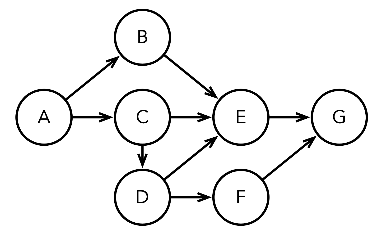 65 |
66 | ```st
67 | "First define the nodes and the edges"
68 | nodes := #( $A $B $C $D $E $F $G ).
69 | edges := #( #( $A $B ) #( $A $C ) #( $B $E ) #( $C $E ) #( $C $D )
70 | #( $D $E ) #( $D $F ) #( $E $G ) #( $F $G ) ).
71 |
72 | "Instantiate the graph algorithm"
73 | topSortingAlgo := AITopologicalSorting new.
74 |
75 | "Set the nodes and edges"
76 | topSortingAlgo nodes: nodes.
77 | topSortingAlgo
78 | edges: edges
79 | from: [ :each | each first ]
80 | to: [ :each | each second ].
81 |
82 | "Run to obtain the result"
83 | topologicalSortedElements := topSortingAlgo run.
84 | ```
85 |
86 | Or if we want to find the shortest path in a weighted graph:
87 |
88 |
65 |
66 | ```st
67 | "First define the nodes and the edges"
68 | nodes := #( $A $B $C $D $E $F $G ).
69 | edges := #( #( $A $B ) #( $A $C ) #( $B $E ) #( $C $E ) #( $C $D )
70 | #( $D $E ) #( $D $F ) #( $E $G ) #( $F $G ) ).
71 |
72 | "Instantiate the graph algorithm"
73 | topSortingAlgo := AITopologicalSorting new.
74 |
75 | "Set the nodes and edges"
76 | topSortingAlgo nodes: nodes.
77 | topSortingAlgo
78 | edges: edges
79 | from: [ :each | each first ]
80 | to: [ :each | each second ].
81 |
82 | "Run to obtain the result"
83 | topologicalSortedElements := topSortingAlgo run.
84 | ```
85 |
86 | Or if we want to find the shortest path in a weighted graph:
87 |
88 | 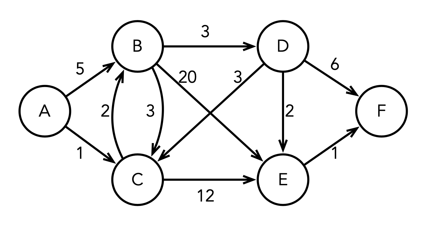 89 |
90 | ```st
91 | nodes := $A to: $F.
92 | edges := #( #( $A $B 5 ) #( $A $C 1 ) #( $B $C 2 ) #( $B $E 20 )
93 | #( $B $D 3 ) #( $C $B 3 ) #( $C $E 12 ) #( $D $C 3 )
94 | #( $D $E 2 ) #( $D $F 6 ) #( $E $F 1 ) ).
95 |
96 | dijkstra := AIDijkstra new.
97 | dijkstra nodes: nodes.
98 | dijkstra
99 | edges: edges
100 | from: [ :each | each first ]
101 | to: [ :each | each second ]
102 | weight: [ :each | each third ].
103 |
104 | shortestPathAToB := dijkstra runFrom: $A to: $B.
105 | pathDistanceAToB := (dijkstra findNode: $B) pathDistance.
106 |
107 | dijkstra end: $F.
108 | shortestPathAToF := dijkstra reconstructPath.
109 | pathDistanceAToF := (dijkstra findNode: $F) pathDistance.
110 |
111 | dijkstra reset.
112 | shortestPathBToE := dijkstra runFrom: $B to: $E.
113 | ```
114 |
115 | ## Graph generation algorithms
116 |
117 | This library also contains algorithms for generating regular and random graphs. This algorithms are not loaded by default. To load them, you can either load them manually using [Iceberg directly from the Pharo image](https://github.com/pharo-vcs/iceberg/wiki/Tutorial) or load the `GraphGenerators` baseline group.
118 |
119 | The algorithms implemented are:
120 |
121 | - Albert Barabasi Graph Generator
122 | - Atlas Graph Graph Generator
123 | - Erdos Renyi GNM Graph Generator
124 | - Erdos Renyi GNP Graph Generator
125 | - Grid 2D Graph Generator
126 | - Grid 3D Graph Generator
127 | - Hexagonal Lattice Graph Generator
128 | - Kleinberg Graph Generator
129 | - Triangular Lattice Graph Generator
130 | - Waltz Strogatz Graph Generator
131 |
132 | ## Comparison of the implemented algorithms
133 |
134 | This section summarizes for each provided graph algorithm in the library its input, its output, some remark and the implemented time complexity.
135 |
136 | **Abbreviations**: DAG means Directed Acyclic Graph, DCG means Directed Cyclic Graph, DG means DG Directed Graph (cyclic or not). V represents the number of vertices and E the number of edges.
137 |
138 | ### Topological sorting
139 |
140 | | Algorithm | Input | Output | Remark | Complexity |
141 | | --------- | ----- | ------------ | ---------------------- | ---------- |
142 | | Kahn's | DAG | sorted nodes | working list iteration | O(V + E) |
143 |
144 | ### Shortest path
145 |
146 | | Algorithm | Input | Output | Remark | Complexity |
147 | | -------------- | --------------------------------------------------- | --------------------------- | --------------------------------------------------------------------------------------------------------------------------- | -------------- |
148 | | BFS | unweighted graph and starting node | path nodes | BFS in queue | O(V + E) |
149 | | DFS | unweighted graph and starting node | path nodes | DFS in queue | O(V + E) |
150 | | Dijkstra's | graph with non-negative weights and starting node | path nodes | [dynamic programming](https://en.wikipedia.org/wiki/Dynamic_programming#Dijkstra's_algorithm_for_the_shortest_path_problem) | O(V²) |
151 | | in DAG | weighted DAG and starting node | path nodes | based on topological sorting | O(V + E) |
152 | | Bellman-Ford | weighted graph and starting node | path nodes | edge [relaxation](https://en.wikipedia.org/wiki/Relaxation_(iterative_method)); detects negative cycles | O(V \* E) |
153 | | Floyd-Warshall | weighted graph | path for every node pair | data structure: two matrices; detects negative cycles | O(V³) |
154 | | A* | graph with non-negative weights, start and end node | path from start to end node | Extension of Dijkstra's algorithm | O(E \* log(V)) |
155 |
156 | ### Strongly connected components
157 |
158 | | Algorithm | Input | Output | Remark | Complexity |
159 | | ------------- | ------------------------- | ------------------------------ | ------------------------------- | ---------- |
160 | | Tarjan's | unweighted graph | list of node lists | based on DFS | O(V + E) |
161 | | Graph Reducer | Tarjan's algorithm output | nodes of the new reduced graph | no default reduction of weights | ? |
162 |
163 | ### Maximum flow
164 |
165 | | Algorithm | Input | Output | Remark | Complexity |
166 | | ------------ | -------------------------------------- | ------------------ | ---------------- | ---------- |
167 | | Edmonds-Karp | weighted DG, source node and sink node | maximal flow value | uses BFS | O(V * E²) |
168 | | Dinic's | weighted DG, source node and sink node | maximal flow value | layering concept | O(V² \* E) |
169 |
170 | ### Link analysis
171 |
172 | | Algorithm | Input | Output | Remark | Complexity |
173 | | --------- | ----- | -------------------------------------------- | --------------------------------------- | ---------- |
174 | | HITS | DG | hub score and authority score for every node | optional weights to improve performance | O(V + E) |
175 |
176 | ### Minimum spanning tree
177 |
178 | | Algorithm | Input | Output | Remark | Complexity |
179 | | --------- | ------------------------------------------------ | -------------------------------- | ---------------------------------------------------------------------------------------- | ---------------- |
180 | | Kruskal’s | undirected weighted graph (non-negative weights) | subset of edges (tree or forest) | [disjoint-set data structure](https://en.wikipedia.org/wiki/Disjoint-set_data_structure) | O(V \* log(E)) |
181 | | Prim’s | connected undirected weighted graph | subset of edges (tree) | very similar to Dijkstra's algorithm | O( V \* (V + E)) |
182 |
183 | Both algorithms are [greedy](https://en.wikipedia.org/wiki/Greedy_algorithm).
184 |
185 | ### Matching
186 |
187 | | Problem | Algorithm | Input | Output | Remark | Complexity |
188 | | ---------------- | -------------- | ----------------------------------------------------------- | ------------------------------------------------ | ---------------------------------- | -------------- |
189 | | Maximum Matching | Graph Matching | undirected weighted graph | independent edges set | greedy approximation | O(E \* log(V)) |
190 | | Stable Matching | Gale-Shapely's | nodes in group A or B with preferences over the other group | set of edges, each one relating a different pair | groups A and B are of equal size n | O(n²) |
191 |
192 | ## External links
193 |
194 | Almost all items are well described in Wikipedia. For a couple of items, the posts in [w3schools](https://www.w3schools.com), [Research Scientist Pod](https://researchdatapod.com) and [Jiho's Blog](https://berryjune07.github.io/computer-science) are outstanding.
195 |
196 | ### Graph problems
197 |
198 | - Topological sorting: [Wikipedia](https://en.wikipedia.org/wiki/Topological_sorting)
199 |
200 | - Shortest path: [Wikipedia](https://en.wikipedia.org/wiki/Shortest_path_problem), [comparison between algorithms](https://www.geeksforgeeks.org/dsa/comparison-between-shortest-path-algorithms/)
201 |
202 | - Minimum spanning tree: [Wikipedia](https://en.wikipedia.org/wiki/Minimum_spanning_tree), [Jiho's Blog](https://berryjune07.github.io/computer-science/minimum-spanning-tree.html), [Prim's vs Kruskal's (Geeks for geeks)](https://www.geeksforgeeks.org/dsa/difference-between-prims-and-kruskals-algorithm-for-mst), [Prim's vs Kruskal's (Baeldung)](https://www.baeldung.com/cs/kruskals-vs-prims-algorithm)
203 |
204 | - Strongly connected components: [Wikipedia](https://en.wikipedia.org/wiki/Strongly_connected_component)
205 |
206 | - Maximum flow: [Wikipedia](https://en.wikipedia.org/wiki/Maximum_flow_problem)
207 |
208 | - Link analysis: [Wikipedia](https://en.wikipedia.org/wiki/Link_analysis)
209 |
210 | - Matching: [Wikipedia](https://en.wikipedia.org/wiki/Matching_(graph_theory)), [Brilliant course](https://brilliant.org/wiki/matching-algorithms)
211 |
212 | ### Graph algorithms
213 |
214 | - A*: [Wikipedia](https://en.wikipedia.org/wiki/A*_search_algorithm), [Reserch Scientist Pod](https://researchdatapod.com/a-star-algorithm/)
215 |
216 | - Bellman-Ford: [Wikipedia](https://en.wikipedia.org/wiki/Bellman–Ford_algorithm), [w3schools](https://www.w3schools.com/dsa/dsa_algo_graphs_bellmanford.php), [Research Scientist Pod](https://researchdatapod.com/bellman-ford-algorithm/), [Jiho's Blog](https://berryjune07.github.io/computer-science/bellman-ford-algorithm.html)
217 |
218 | - BFS vs. DFS: [Wikipedia (BFS)](https://en.wikipedia.org/wiki/Breadth-first_search), [Wikipedia (DFS)](https://en.wikipedia.org/wiki/Depth-first_search), [wscubetech](https://www.wscubetech.com/resources/dsa/dfs-vs-bfs), [Baeldung](https://www.baeldung.com/cs/dfs-vs-bfs), [Jiho's Blog](https://berryjune07.github.io/computer-science/dfs-and-bfs.html), [IntelliPaat](https://intellipaat.com/blog/difference-between-bfs-and-dfs/), [codecademy](https://www.codecademy.com/article/bfs-vs-dfs)
219 |
220 | - Dijkstra's: [Wikipedia](https://en.wikipedia.org/wiki/Dijkstra%27s_algorithm), [w3schools](https://www.w3schools.com/dsa/dsa_algo_graphs_dijkstra.php), [Research Scientist Pod](https://researchdatapod.com/dijkstras-algorithm/)
221 |
222 | - Dinic's: [Wikipedia](https://en.wikipedia.org/wiki/Dinic%27s_algorithm), [Geeks for geeks](https://www.geeksforgeeks.org/dsa/dinics-algorithm-maximum-flow)
223 |
224 | - Edmonds-Karp: [Wikipedia](https://en.wikipedia.org/wiki/Edmonds–Karp_algorithm)
225 |
226 | - Floyd-Warshall: [Wikipedia](https://en.wikipedia.org/wiki/Floyd–Warshall_algorithm), [Research Scientist Pod](https://researchdatapod.com/floyd-warshall-algorithm/), [Jiho's Blog](https://berryjune07.github.io/computer-science/floyd-warshall-algorithm.html)
227 |
228 | - Gale-Shapely: [Wikipedia](https://de.wikipedia.org/wiki/Stable_Marriage_Problem#Gale-Shapley-Algorithmus)
229 |
230 | - HITS: [Wikipedia](https://en.wikipedia.org/wiki/HITS_algorithm)
231 |
232 | - Kahn's: [Wikipedia](https://en.wikipedia.org/wiki/Topological_sorting#Kahn's_algorithm)
233 |
234 | - Kruskal’s: [Wikipedia](https://en.wikipedia.org/wiki/Kruskal%27s_algorithm)
235 |
236 | - Disjoint-Set data structure: [Wikipedia](https://en.wikipedia.org/wiki/Disjoint-set_data_structure)
237 |
238 | - Disjoint-Set Forest: [Jiho's Blog](https://berryjune07.github.io/computer-science/disjoint-set-forest.html)
239 |
240 | - Matching Approximation: [Cornell lecture](https://www.cs.cornell.edu/courses/cs6820/2014fa/matchingNotes.pdf)
241 |
242 | - Prim's: [Wikipedia](https://en.wikipedia.org/wiki/Prim%27s_algorithm)
243 |
244 | - Tarjan's: [Wikipedia](https://en.wikipedia.org/wiki/Tarjan%27s_strongly_connected_components_algorithm), [dev.to](https://dev.to/muhammad_taaha_90438c47f1/understanding-tarjans-algorithm-with-visual-examples-5hb8)
245 |
--------------------------------------------------------------------------------
89 |
90 | ```st
91 | nodes := $A to: $F.
92 | edges := #( #( $A $B 5 ) #( $A $C 1 ) #( $B $C 2 ) #( $B $E 20 )
93 | #( $B $D 3 ) #( $C $B 3 ) #( $C $E 12 ) #( $D $C 3 )
94 | #( $D $E 2 ) #( $D $F 6 ) #( $E $F 1 ) ).
95 |
96 | dijkstra := AIDijkstra new.
97 | dijkstra nodes: nodes.
98 | dijkstra
99 | edges: edges
100 | from: [ :each | each first ]
101 | to: [ :each | each second ]
102 | weight: [ :each | each third ].
103 |
104 | shortestPathAToB := dijkstra runFrom: $A to: $B.
105 | pathDistanceAToB := (dijkstra findNode: $B) pathDistance.
106 |
107 | dijkstra end: $F.
108 | shortestPathAToF := dijkstra reconstructPath.
109 | pathDistanceAToF := (dijkstra findNode: $F) pathDistance.
110 |
111 | dijkstra reset.
112 | shortestPathBToE := dijkstra runFrom: $B to: $E.
113 | ```
114 |
115 | ## Graph generation algorithms
116 |
117 | This library also contains algorithms for generating regular and random graphs. This algorithms are not loaded by default. To load them, you can either load them manually using [Iceberg directly from the Pharo image](https://github.com/pharo-vcs/iceberg/wiki/Tutorial) or load the `GraphGenerators` baseline group.
118 |
119 | The algorithms implemented are:
120 |
121 | - Albert Barabasi Graph Generator
122 | - Atlas Graph Graph Generator
123 | - Erdos Renyi GNM Graph Generator
124 | - Erdos Renyi GNP Graph Generator
125 | - Grid 2D Graph Generator
126 | - Grid 3D Graph Generator
127 | - Hexagonal Lattice Graph Generator
128 | - Kleinberg Graph Generator
129 | - Triangular Lattice Graph Generator
130 | - Waltz Strogatz Graph Generator
131 |
132 | ## Comparison of the implemented algorithms
133 |
134 | This section summarizes for each provided graph algorithm in the library its input, its output, some remark and the implemented time complexity.
135 |
136 | **Abbreviations**: DAG means Directed Acyclic Graph, DCG means Directed Cyclic Graph, DG means DG Directed Graph (cyclic or not). V represents the number of vertices and E the number of edges.
137 |
138 | ### Topological sorting
139 |
140 | | Algorithm | Input | Output | Remark | Complexity |
141 | | --------- | ----- | ------------ | ---------------------- | ---------- |
142 | | Kahn's | DAG | sorted nodes | working list iteration | O(V + E) |
143 |
144 | ### Shortest path
145 |
146 | | Algorithm | Input | Output | Remark | Complexity |
147 | | -------------- | --------------------------------------------------- | --------------------------- | --------------------------------------------------------------------------------------------------------------------------- | -------------- |
148 | | BFS | unweighted graph and starting node | path nodes | BFS in queue | O(V + E) |
149 | | DFS | unweighted graph and starting node | path nodes | DFS in queue | O(V + E) |
150 | | Dijkstra's | graph with non-negative weights and starting node | path nodes | [dynamic programming](https://en.wikipedia.org/wiki/Dynamic_programming#Dijkstra's_algorithm_for_the_shortest_path_problem) | O(V²) |
151 | | in DAG | weighted DAG and starting node | path nodes | based on topological sorting | O(V + E) |
152 | | Bellman-Ford | weighted graph and starting node | path nodes | edge [relaxation](https://en.wikipedia.org/wiki/Relaxation_(iterative_method)); detects negative cycles | O(V \* E) |
153 | | Floyd-Warshall | weighted graph | path for every node pair | data structure: two matrices; detects negative cycles | O(V³) |
154 | | A* | graph with non-negative weights, start and end node | path from start to end node | Extension of Dijkstra's algorithm | O(E \* log(V)) |
155 |
156 | ### Strongly connected components
157 |
158 | | Algorithm | Input | Output | Remark | Complexity |
159 | | ------------- | ------------------------- | ------------------------------ | ------------------------------- | ---------- |
160 | | Tarjan's | unweighted graph | list of node lists | based on DFS | O(V + E) |
161 | | Graph Reducer | Tarjan's algorithm output | nodes of the new reduced graph | no default reduction of weights | ? |
162 |
163 | ### Maximum flow
164 |
165 | | Algorithm | Input | Output | Remark | Complexity |
166 | | ------------ | -------------------------------------- | ------------------ | ---------------- | ---------- |
167 | | Edmonds-Karp | weighted DG, source node and sink node | maximal flow value | uses BFS | O(V * E²) |
168 | | Dinic's | weighted DG, source node and sink node | maximal flow value | layering concept | O(V² \* E) |
169 |
170 | ### Link analysis
171 |
172 | | Algorithm | Input | Output | Remark | Complexity |
173 | | --------- | ----- | -------------------------------------------- | --------------------------------------- | ---------- |
174 | | HITS | DG | hub score and authority score for every node | optional weights to improve performance | O(V + E) |
175 |
176 | ### Minimum spanning tree
177 |
178 | | Algorithm | Input | Output | Remark | Complexity |
179 | | --------- | ------------------------------------------------ | -------------------------------- | ---------------------------------------------------------------------------------------- | ---------------- |
180 | | Kruskal’s | undirected weighted graph (non-negative weights) | subset of edges (tree or forest) | [disjoint-set data structure](https://en.wikipedia.org/wiki/Disjoint-set_data_structure) | O(V \* log(E)) |
181 | | Prim’s | connected undirected weighted graph | subset of edges (tree) | very similar to Dijkstra's algorithm | O( V \* (V + E)) |
182 |
183 | Both algorithms are [greedy](https://en.wikipedia.org/wiki/Greedy_algorithm).
184 |
185 | ### Matching
186 |
187 | | Problem | Algorithm | Input | Output | Remark | Complexity |
188 | | ---------------- | -------------- | ----------------------------------------------------------- | ------------------------------------------------ | ---------------------------------- | -------------- |
189 | | Maximum Matching | Graph Matching | undirected weighted graph | independent edges set | greedy approximation | O(E \* log(V)) |
190 | | Stable Matching | Gale-Shapely's | nodes in group A or B with preferences over the other group | set of edges, each one relating a different pair | groups A and B are of equal size n | O(n²) |
191 |
192 | ## External links
193 |
194 | Almost all items are well described in Wikipedia. For a couple of items, the posts in [w3schools](https://www.w3schools.com), [Research Scientist Pod](https://researchdatapod.com) and [Jiho's Blog](https://berryjune07.github.io/computer-science) are outstanding.
195 |
196 | ### Graph problems
197 |
198 | - Topological sorting: [Wikipedia](https://en.wikipedia.org/wiki/Topological_sorting)
199 |
200 | - Shortest path: [Wikipedia](https://en.wikipedia.org/wiki/Shortest_path_problem), [comparison between algorithms](https://www.geeksforgeeks.org/dsa/comparison-between-shortest-path-algorithms/)
201 |
202 | - Minimum spanning tree: [Wikipedia](https://en.wikipedia.org/wiki/Minimum_spanning_tree), [Jiho's Blog](https://berryjune07.github.io/computer-science/minimum-spanning-tree.html), [Prim's vs Kruskal's (Geeks for geeks)](https://www.geeksforgeeks.org/dsa/difference-between-prims-and-kruskals-algorithm-for-mst), [Prim's vs Kruskal's (Baeldung)](https://www.baeldung.com/cs/kruskals-vs-prims-algorithm)
203 |
204 | - Strongly connected components: [Wikipedia](https://en.wikipedia.org/wiki/Strongly_connected_component)
205 |
206 | - Maximum flow: [Wikipedia](https://en.wikipedia.org/wiki/Maximum_flow_problem)
207 |
208 | - Link analysis: [Wikipedia](https://en.wikipedia.org/wiki/Link_analysis)
209 |
210 | - Matching: [Wikipedia](https://en.wikipedia.org/wiki/Matching_(graph_theory)), [Brilliant course](https://brilliant.org/wiki/matching-algorithms)
211 |
212 | ### Graph algorithms
213 |
214 | - A*: [Wikipedia](https://en.wikipedia.org/wiki/A*_search_algorithm), [Reserch Scientist Pod](https://researchdatapod.com/a-star-algorithm/)
215 |
216 | - Bellman-Ford: [Wikipedia](https://en.wikipedia.org/wiki/Bellman–Ford_algorithm), [w3schools](https://www.w3schools.com/dsa/dsa_algo_graphs_bellmanford.php), [Research Scientist Pod](https://researchdatapod.com/bellman-ford-algorithm/), [Jiho's Blog](https://berryjune07.github.io/computer-science/bellman-ford-algorithm.html)
217 |
218 | - BFS vs. DFS: [Wikipedia (BFS)](https://en.wikipedia.org/wiki/Breadth-first_search), [Wikipedia (DFS)](https://en.wikipedia.org/wiki/Depth-first_search), [wscubetech](https://www.wscubetech.com/resources/dsa/dfs-vs-bfs), [Baeldung](https://www.baeldung.com/cs/dfs-vs-bfs), [Jiho's Blog](https://berryjune07.github.io/computer-science/dfs-and-bfs.html), [IntelliPaat](https://intellipaat.com/blog/difference-between-bfs-and-dfs/), [codecademy](https://www.codecademy.com/article/bfs-vs-dfs)
219 |
220 | - Dijkstra's: [Wikipedia](https://en.wikipedia.org/wiki/Dijkstra%27s_algorithm), [w3schools](https://www.w3schools.com/dsa/dsa_algo_graphs_dijkstra.php), [Research Scientist Pod](https://researchdatapod.com/dijkstras-algorithm/)
221 |
222 | - Dinic's: [Wikipedia](https://en.wikipedia.org/wiki/Dinic%27s_algorithm), [Geeks for geeks](https://www.geeksforgeeks.org/dsa/dinics-algorithm-maximum-flow)
223 |
224 | - Edmonds-Karp: [Wikipedia](https://en.wikipedia.org/wiki/Edmonds–Karp_algorithm)
225 |
226 | - Floyd-Warshall: [Wikipedia](https://en.wikipedia.org/wiki/Floyd–Warshall_algorithm), [Research Scientist Pod](https://researchdatapod.com/floyd-warshall-algorithm/), [Jiho's Blog](https://berryjune07.github.io/computer-science/floyd-warshall-algorithm.html)
227 |
228 | - Gale-Shapely: [Wikipedia](https://de.wikipedia.org/wiki/Stable_Marriage_Problem#Gale-Shapley-Algorithmus)
229 |
230 | - HITS: [Wikipedia](https://en.wikipedia.org/wiki/HITS_algorithm)
231 |
232 | - Kahn's: [Wikipedia](https://en.wikipedia.org/wiki/Topological_sorting#Kahn's_algorithm)
233 |
234 | - Kruskal’s: [Wikipedia](https://en.wikipedia.org/wiki/Kruskal%27s_algorithm)
235 |
236 | - Disjoint-Set data structure: [Wikipedia](https://en.wikipedia.org/wiki/Disjoint-set_data_structure)
237 |
238 | - Disjoint-Set Forest: [Jiho's Blog](https://berryjune07.github.io/computer-science/disjoint-set-forest.html)
239 |
240 | - Matching Approximation: [Cornell lecture](https://www.cs.cornell.edu/courses/cs6820/2014fa/matchingNotes.pdf)
241 |
242 | - Prim's: [Wikipedia](https://en.wikipedia.org/wiki/Prim%27s_algorithm)
243 |
244 | - Tarjan's: [Wikipedia](https://en.wikipedia.org/wiki/Tarjan%27s_strongly_connected_components_algorithm), [dev.to](https://dev.to/muhammad_taaha_90438c47f1/understanding-tarjans-algorithm-with-visual-examples-5hb8)
245 |
--------------------------------------------------------------------------------