├── .gitignore
├── .github
├── .gitignore
├── ISSUE_TEMPLATE
│ └── bug_report.md
└── workflows
│ ├── check.yaml
│ └── pkgdown.yaml
├── tests
├── testthat.R
└── testthat
│ ├── test-scDblFinder.R
│ ├── test-recoverDoublets.R
│ ├── test-findDoubletClusters.R
│ └── test-computeDoubletDensity.R
├── .Rbuildignore
├── inst
├── docs
│ └── scDblFinder_comparison.png
├── extdata
│ └── example_fragments.tsv.gz
├── CITATION
└── NEWS
├── _pkgdown.yml
├── Dockerfile
├── man
├── propHomotypic.Rd
├── TFIDF.Rd
├── getExpectedDoublets.Rd
├── plotThresholds.Rd
├── mockDoubletSCE.Rd
├── getCellPairs.Rd
├── addDoublets.Rd
├── selFeatures.Rd
├── clusterStickiness.Rd
├── cxds2.Rd
├── plotDoubletMap.Rd
├── doubletPairwiseEnrichment.Rd
├── amulet.Rd
├── createDoublets.Rd
├── fastcluster.Rd
├── aggregateFeatures.Rd
├── clamulet.Rd
├── directDblClassification.Rd
├── amuletFromCounts.Rd
├── doubletThresholding.Rd
├── getArtificialDoublets.Rd
├── getFragmentOverlaps.Rd
├── recoverDoublets.Rd
├── computeDoubletDensity.Rd
├── findDoubletClusters.Rd
└── scDblFinder.Rd
├── DESCRIPTION
├── R
├── clustering.R
├── atac_processing.R
├── plotting.R
├── enrichment.R
├── recoverDoublets.R
├── getFragmentOverlaps.R
├── computeDoubletDensity.R
├── findDoubletClusters.R
└── doubletThresholding.R
├── vignettes
├── recoverDoublets.Rmd
├── introduction.Rmd
├── computeDoubletDensity.Rmd
├── findDoubletClusters.Rmd
└── scATAC.Rmd
├── NAMESPACE
└── README.md
/.gitignore:
--------------------------------------------------------------------------------
1 | docs
2 |
--------------------------------------------------------------------------------
/.github/.gitignore:
--------------------------------------------------------------------------------
1 | *.html
2 |
--------------------------------------------------------------------------------
/tests/testthat.R:
--------------------------------------------------------------------------------
1 | library(testthat)
2 | library(scDblFinder)
3 | test_check("scDblFinder")
4 |
--------------------------------------------------------------------------------
/.Rbuildignore:
--------------------------------------------------------------------------------
1 | ^\.github$
2 | ^.*\.Rproj$
3 | ^\.Rproj\.user$
4 | ^_pkgdown\.yml$
5 | ^docs$
6 | ^pkgdown$
7 |
--------------------------------------------------------------------------------
/inst/docs/scDblFinder_comparison.png:
--------------------------------------------------------------------------------
https://raw.githubusercontent.com/plger/scDblFinder/HEAD/inst/docs/scDblFinder_comparison.png
--------------------------------------------------------------------------------
/inst/extdata/example_fragments.tsv.gz:
--------------------------------------------------------------------------------
https://raw.githubusercontent.com/plger/scDblFinder/HEAD/inst/extdata/example_fragments.tsv.gz
--------------------------------------------------------------------------------
/_pkgdown.yml:
--------------------------------------------------------------------------------
1 | url: https://plger.github.io/scDblFinder/
2 | template:
3 | bootstrap: 5
4 | bootswatch: cyborg
5 | theme: arrow-dark
6 |
7 |
--------------------------------------------------------------------------------
/Dockerfile:
--------------------------------------------------------------------------------
1 | FROM bioconductor/bioconductor_docker:devel
2 |
3 | MAINTAINER pl.germain@gmail.com
4 |
5 | WORKDIR /home/build/package
6 |
7 | COPY . /home/build/package
8 |
9 | ENV R_REMOTES_NO_ERRORS_FROM_WARNINGS=true
10 |
11 | RUN Rscript -e "BiocManager::install('ensembldb'); BiocManager::install('Rtsne')"
12 | RUN Rscript -e "devtools::install('.', dependencies=TRUE, repos = BiocManager::repositories(), build_vignettes = TRUE)"
13 |
--------------------------------------------------------------------------------
/inst/CITATION:
--------------------------------------------------------------------------------
1 | bibentry(bibtype = "Article",
2 | title = "Doublet identification in single-cell sequencing data using scDblFinder",
3 | author = c(person("Pierre-Luc", "Germain"),
4 | person("Aaron", "Lun"),
5 | person("Carlos", "Garcia Meixide"),
6 | person("Will", "Macnair"),
7 | person("Mark D.", "Robinson")),
8 | year = 2022,
9 | journal = "f1000research",
10 | doi = "10.12688/f1000research.73600.2"
11 | )
12 |
--------------------------------------------------------------------------------
/man/propHomotypic.Rd:
--------------------------------------------------------------------------------
1 | % Generated by roxygen2: do not edit by hand
2 | % Please edit documentation in R/misc.R
3 | \name{propHomotypic}
4 | \alias{propHomotypic}
5 | \title{propHomotypic}
6 | \usage{
7 | propHomotypic(clusters)
8 | }
9 | \arguments{
10 | \item{clusters}{A vector of cluster labels}
11 | }
12 | \value{
13 | A numeric value between 0 and 1.
14 | }
15 | \description{
16 | Computes the proportion of pairs expected to be made of elements from the
17 | same cluster.
18 | }
19 | \examples{
20 | clusters <- sample(LETTERS[1:5], 100, replace=TRUE)
21 | propHomotypic(clusters)
22 | }
23 |
--------------------------------------------------------------------------------
/man/TFIDF.Rd:
--------------------------------------------------------------------------------
1 | % Generated by roxygen2: do not edit by hand
2 | % Please edit documentation in R/atac_processing.R
3 | \name{TFIDF}
4 | \alias{TFIDF}
5 | \title{TFIDF}
6 | \usage{
7 | TFIDF(x, sf = 10000)
8 | }
9 | \arguments{
10 | \item{x}{The matrix of occurrences}
11 |
12 | \item{sf}{Scaling factor}
13 | }
14 | \value{
15 | An array of same dimensions as `x`
16 | }
17 | \description{
18 | The Term Frequency - Inverse Document Frequency (TF-IDF) normalization, as
19 | implemented in Stuart & Butler et al. 2019.
20 | }
21 | \examples{
22 | m <- matrix(rpois(500,1),nrow=50)
23 | m <- TFIDF(m)
24 | }
25 |
--------------------------------------------------------------------------------
/.github/ISSUE_TEMPLATE/bug_report.md:
--------------------------------------------------------------------------------
1 | ---
2 | name: Bug report
3 | about: Create a report to help us improve
4 | title: ''
5 | labels: ''
6 | assignees: ''
7 |
8 | ---
9 |
10 | **Describe the bug**
11 | A clear and concise description of what the bug is.
12 |
13 | **MRE -- Minimal example to reproduce the bug**
14 | Steps to reproduce the behavior, eventually with a dataset if it's dataset-specific. If possible, try to reproduce the error with a single sample and/or without multithreading.
15 |
16 | **Traceback**
17 | If the issue triggers an R error (rather than, say, unexpected results), please provide the output of `traceback()` right after the error occurs.
18 |
19 | **Session info**
20 | Provide the output of `sessionInfo()`.
21 |
22 | Before posting your issue, please ensure that it is reproducible with a recent Bioconductor and `scDblFinder` version.
23 |
--------------------------------------------------------------------------------
/man/getExpectedDoublets.Rd:
--------------------------------------------------------------------------------
1 | % Generated by roxygen2: do not edit by hand
2 | % Please edit documentation in R/misc.R
3 | \name{getExpectedDoublets}
4 | \alias{getExpectedDoublets}
5 | \title{getExpectedDoublets}
6 | \usage{
7 | getExpectedDoublets(x, dbr = NULL, only.heterotypic = TRUE, dbr.per1k = 0.008)
8 | }
9 | \arguments{
10 | \item{x}{A vector of cluster labels for each cell}
11 |
12 | \item{dbr}{The expected doublet rate.}
13 |
14 | \item{only.heterotypic}{Logical; whether to return expectations only for
15 | heterotypic doublets}
16 |
17 | \item{dbr.per1k}{The expected proportion of doublets per 1000 cells.}
18 | }
19 | \value{
20 | The expected number of doublets of each combination of clusters
21 | }
22 | \description{
23 | getExpectedDoublets
24 | }
25 | \examples{
26 | # random cluster labels
27 | cl <- sample(head(LETTERS,4), size=2000, prob=c(.4,.2,.2,.2), replace=TRUE)
28 | getExpectedDoublets(cl)
29 | }
30 |
--------------------------------------------------------------------------------
/man/plotThresholds.Rd:
--------------------------------------------------------------------------------
1 | % Generated by roxygen2: do not edit by hand
2 | % Please edit documentation in R/plotting.R
3 | \name{plotThresholds}
4 | \alias{plotThresholds}
5 | \title{plotThresholds}
6 | \usage{
7 | plotThresholds(d, ths = (0:100)/100, dbr = NULL, dbr.sd = NULL, do.plot = TRUE)
8 | }
9 | \arguments{
10 | \item{d}{A data.frame of cell properties, with each row representing a cell,
11 | as produced by `scDblFinder(..., returnType="table")`.}
12 |
13 | \item{ths}{A vector of thresholds between 0 and 1 at which to plot values.}
14 |
15 | \item{dbr}{The expected (mean) doublet rate.}
16 |
17 | \item{dbr.sd}{The standard deviation of the doublet rate, representing the
18 | uncertainty in the estimate.}
19 |
20 | \item{do.plot}{Logical; whether to plot the data (otherwise will return the
21 | underlying data.frame).}
22 | }
23 | \value{
24 | A ggplot, or a data.frame if `do.plot==FALSE`.
25 | }
26 | \description{
27 | Plots scores used for thresholding.
28 | }
29 |
--------------------------------------------------------------------------------
/man/mockDoubletSCE.Rd:
--------------------------------------------------------------------------------
1 | % Generated by roxygen2: do not edit by hand
2 | % Please edit documentation in R/misc.R
3 | \name{mockDoubletSCE}
4 | \alias{mockDoubletSCE}
5 | \title{mockDoubletSCE}
6 | \usage{
7 | mockDoubletSCE(
8 | ncells = c(200, 300),
9 | ngenes = 200,
10 | mus = NULL,
11 | dbl.rate = 0.1,
12 | only.heterotypic = TRUE
13 | )
14 | }
15 | \arguments{
16 | \item{ncells}{A positive integer vector indicating the number of cells per
17 | cluster (min 2 clusters)}
18 |
19 | \item{ngenes}{The number of genes to simulate. Ignored if `mus` is given.}
20 |
21 | \item{mus}{A list of cluster averages.}
22 |
23 | \item{dbl.rate}{The doublet rate}
24 |
25 | \item{only.heterotypic}{Whether to create only heterotypic doublets}
26 | }
27 | \value{
28 | A SingleCellExperiment object, with the colData columns `type`
29 | indicating whether the cell is a singlet or doublet, and `cluster`
30 | indicating from which cluster (or cluster combination) it was simulated.
31 | }
32 | \description{
33 | Creates a mock random single-cell experiment object with doublets
34 | }
35 | \examples{
36 | sce <- mockDoubletSCE()
37 | }
38 |
--------------------------------------------------------------------------------
/man/getCellPairs.Rd:
--------------------------------------------------------------------------------
1 | % Generated by roxygen2: do not edit by hand
2 | % Please edit documentation in R/getArtificialDoublets.R
3 | \name{getCellPairs}
4 | \alias{getCellPairs}
5 | \title{getCellPairs}
6 | \usage{
7 | getCellPairs(
8 | clusters,
9 | n = 1000,
10 | ls = NULL,
11 | q = c(0.1, 0.9),
12 | selMode = "proportional",
13 | soft.min = 5
14 | )
15 | }
16 | \arguments{
17 | \item{clusters}{A vector of cluster labels for each cell, or a list containing
18 | metacells and graph}
19 |
20 | \item{n}{The number of cell pairs to obtain}
21 |
22 | \item{ls}{Optional library sizes}
23 |
24 | \item{q}{Library size quantiles between which to include cells (ignored if
25 | `ls` is NULL)}
26 |
27 | \item{selMode}{How to decide the number of pairs of each kind to produce.
28 | Either 'proportional' (default, proportional to the abundance of the
29 | underlying clusters), 'uniform' or 'sqrt'.}
30 |
31 | \item{soft.min}{Minimum number of pairs of a given type.}
32 | }
33 | \value{
34 | A data.frame with the columns
35 | }
36 | \description{
37 | Given a vector of cluster labels, returns pairs of cross-cluster cells
38 | }
39 | \examples{
40 | # create random labels
41 | x <- sample(head(LETTERS), 100, replace=TRUE)
42 | getCellPairs(x, n=6)
43 | }
44 |
--------------------------------------------------------------------------------
/.github/workflows/check.yaml:
--------------------------------------------------------------------------------
1 | on:
2 | push:
3 | pull_request:
4 | branches:
5 | - devel
6 | paths-ignore:
7 | - 'README.md'
8 |
9 | name: R-CMD-check
10 |
11 | jobs:
12 | R-CMD-check:
13 | runs-on: ubuntu-latest
14 | container: plger/scdblfinder:latest
15 |
16 | steps:
17 | - name: Check out repo
18 | uses: actions/checkout@v2
19 |
20 | - name: Install latest BiocCheck
21 | run: BiocManager::install(c("BiocCheck"))
22 | shell: Rscript {0}
23 |
24 | - name: Check
25 | env:
26 | _R_CHECK_CRAN_INCOMING_REMOTE_: false
27 | run: rcmdcheck::rcmdcheck(args = "--no-manual", error_on = "error", check_dir = "check")
28 | shell: Rscript {0}
29 |
30 | - name: BiocCheck
31 | run: BiocCheck::BiocCheck(".")
32 | shell: Rscript {0}
33 |
34 | - name: Upload check results
35 | if: failure()
36 | uses: actions/upload-artifact@master
37 | with:
38 | name: ${{ runner.os }}-r${{ matrix.config.r }}-results
39 | path: check
40 |
41 | - name: Show testthat output
42 | if: always()
43 | run: find check -name 'testthat.Rout*' -exec cat '{}' \; || true
44 | shell: bash
45 |
--------------------------------------------------------------------------------
/man/addDoublets.Rd:
--------------------------------------------------------------------------------
1 | % Generated by roxygen2: do not edit by hand
2 | % Please edit documentation in R/getArtificialDoublets.R
3 | \name{addDoublets}
4 | \alias{addDoublets}
5 | \title{addDoublets}
6 | \usage{
7 | addDoublets(
8 | x,
9 | clusters,
10 | dbr = (0.01 * ncol(x)/1000),
11 | only.heterotypic = TRUE,
12 | adjustSize = FALSE,
13 | prefix = "doublet.",
14 | ...
15 | )
16 | }
17 | \arguments{
18 | \item{x}{A count matrix of singlets, or a
19 | \code{\link[SummarizedExperiment]{SummarizedExperiment-class}}}
20 |
21 | \item{clusters}{A vector of cluster labels for each column of `x`}
22 |
23 | \item{dbr}{The doublet rate}
24 |
25 | \item{only.heterotypic}{Whether to add only heterotypic doublets.}
26 |
27 | \item{adjustSize}{Whether to adjust the library sizes of the doublets.}
28 |
29 | \item{prefix}{Prefix for the colnames generated.}
30 |
31 | \item{...}{Any further arguments to \code{\link{createDoublets}}.}
32 | }
33 | \value{
34 | A `SingleCellExperiment` with the colData columns `cluster` and
35 | `type` (indicating whether the cell is a singlet or doublet).
36 | }
37 | \description{
38 | Adds artificial doublets to an existing dataset
39 | }
40 | \examples{
41 | sce <- mockDoubletSCE(dbl.rate=0)
42 | sce <- addDoublets(sce, clusters=sce$cluster)
43 | }
44 |
--------------------------------------------------------------------------------
/man/selFeatures.Rd:
--------------------------------------------------------------------------------
1 | % Generated by roxygen2: do not edit by hand
2 | % Please edit documentation in R/misc.R
3 | \name{selFeatures}
4 | \alias{selFeatures}
5 | \title{selFeatures}
6 | \usage{
7 | selFeatures(
8 | sce,
9 | clusters = NULL,
10 | nfeatures = 1000,
11 | propMarkers = 0,
12 | FDR.max = 0.05
13 | )
14 | }
15 | \arguments{
16 | \item{sce}{A \code{\link[SummarizedExperiment]{SummarizedExperiment-class}},
17 | \code{\link[SingleCellExperiment]{SingleCellExperiment-class}} with a
18 | 'counts' assay.}
19 |
20 | \item{clusters}{Optional cluster assignments. Should either be a vector of
21 | labels for each cell.}
22 |
23 | \item{nfeatures}{The number of features to select.}
24 |
25 | \item{propMarkers}{The proportion of features to select from markers (rather
26 | than on the basis of high expression). Ignored if `clusters` isn't given.}
27 |
28 | \item{FDR.max}{The maximum marker binom FDR to be included in the selection.
29 | (see \code{\link[scran]{findMarkers}}).}
30 | }
31 | \value{
32 | A vector of feature (i.e. row) names.
33 | }
34 | \description{
35 | Selects features based on cluster-wise expression or marker detection, or a
36 | combination.
37 | }
38 | \examples{
39 | sce <- mockDoubletSCE()
40 | selFeatures(sce, clusters=sce$cluster, nfeatures=5)
41 | }
42 |
--------------------------------------------------------------------------------
/man/clusterStickiness.Rd:
--------------------------------------------------------------------------------
1 | % Generated by roxygen2: do not edit by hand
2 | % Please edit documentation in R/enrichment.R
3 | \name{clusterStickiness}
4 | \alias{clusterStickiness}
5 | \title{clusterStickiness}
6 | \usage{
7 | clusterStickiness(
8 | x,
9 | type = c("quasibinomial", "nbinom", "binomial", "poisson"),
10 | inclDiff = NULL,
11 | verbose = TRUE
12 | )
13 | }
14 | \arguments{
15 | \item{x}{A table of double statistics, or a SingleCellExperiment on which
16 | \link{scDblFinder} was run using the cluster-based approach.}
17 |
18 | \item{type}{The type of test to use (quasibinomial recommended).}
19 |
20 | \item{inclDiff}{Logical; whether to include the difficulty in the model. If
21 | NULL, will be used only if there is a significant trend with the enrichment.}
22 |
23 | \item{verbose}{Logical; whether to print additional running information.}
24 | }
25 | \value{
26 | A table of test results for each cluster.
27 | }
28 | \description{
29 | Tests for enrichment of doublets created from each cluster (i.e. cluster's
30 | stickiness). Only applicable with >=4 clusters.
31 | Note that when applied to an multisample object, this functions assumes that
32 | the cluster labels match across samples.
33 | }
34 | \examples{
35 | sce <- mockDoubletSCE(rep(200,5), dbl.rate=0.2)
36 | sce <- scDblFinder(sce, clusters=TRUE, artificialDoublets=500)
37 | clusterStickiness(sce)
38 | }
39 |
--------------------------------------------------------------------------------
/man/cxds2.Rd:
--------------------------------------------------------------------------------
1 | % Generated by roxygen2: do not edit by hand
2 | % Please edit documentation in R/misc.R
3 | \name{cxds2}
4 | \alias{cxds2}
5 | \title{cxds2}
6 | \usage{
7 | cxds2(x, whichDbls = c(), ntop = 500, binThresh = NULL)
8 | }
9 | \arguments{
10 | \item{x}{A matrix of counts, or a `SingleCellExperiment` containing a
11 | 'counts'}
12 |
13 | \item{whichDbls}{The columns of `x` which are known doublets.}
14 |
15 | \item{ntop}{The number of top features to keep.}
16 |
17 | \item{binThresh}{The count threshold to be considered expressed.}
18 | }
19 | \value{
20 | A cxds score or, if `x` is a `SingleCellExperiment`, `x` with an
21 | added `cxds_score` colData column.
22 | }
23 | \description{
24 | Calculates a coexpression-based doublet score using the method developed by
25 | \href{https://doi.org/10.1093/bioinformatics/btz698}{Bais and Kostka 2020}.
26 | This is the original implementation from the
27 | \href{https://www.bioconductor.org/packages/release/bioc/html/scds.html}{scds}
28 | package, but enabling scores to be calculated for all cells while the gene
29 | coexpression is based only on a subset (i.e. excluding known/artificial
30 | doublets) and making it robust to low sparsity.
31 | }
32 | \examples{
33 | sce <- mockDoubletSCE()
34 | sce <- cxds2(sce)
35 | # which is equivalent to
36 | # sce$cxds_score <- cxds2(counts(sce))
37 | }
38 | \references{
39 | \url{https://doi.org/10.1093/bioinformatics/btz698}
40 | }
41 |
--------------------------------------------------------------------------------
/man/plotDoubletMap.Rd:
--------------------------------------------------------------------------------
1 | % Generated by roxygen2: do not edit by hand
2 | % Please edit documentation in R/plotting.R
3 | \name{plotDoubletMap}
4 | \alias{plotDoubletMap}
5 | \title{plotDoubletMap}
6 | \usage{
7 | plotDoubletMap(
8 | sce,
9 | colorBy = "enrichment",
10 | labelBy = "observed",
11 | addSizes = TRUE,
12 | col = NULL,
13 | column_title = "Clusters",
14 | row_title = "Clusters",
15 | column_title_side = "bottom",
16 | na_col = "white",
17 | ...
18 | )
19 | }
20 | \arguments{
21 | \item{sce}{A SingleCellExperiment object on which `scDblFinder` has been run
22 | with the cluster-based approach.}
23 |
24 | \item{colorBy}{Determines the color mapping. Either "enrichment" (for
25 | log2-enrichment over expectation) or any column of
26 | `metadata(sce)$scDblFinder.stats`}
27 |
28 | \item{labelBy}{Determines the cell labels. Either "enrichment" (for
29 | log2-enrichment over expectation) or any column of
30 | `metadata(sce)$scDblFinder.stats`}
31 |
32 | \item{addSizes}{Logical; whether to add the sizes of clusters to labels}
33 |
34 | \item{col}{The colors scale to use (passed to `ComplexHeatmap::Heatmap`)}
35 |
36 | \item{column_title}{passed to `ComplexHeatmap::Heatmap`}
37 |
38 | \item{row_title}{passed to `ComplexHeatmap::Heatmap`}
39 |
40 | \item{column_title_side}{passed to `ComplexHeatmap::Heatmap`}
41 |
42 | \item{na_col}{color for NA cells}
43 |
44 | \item{...}{passed to `ComplexHeatmap::Heatmap`}
45 | }
46 | \value{
47 | a Heatmap object
48 | }
49 | \description{
50 | Plots a heatmap of observed versus expected doublets.
51 | Requires the `ComplexHeatmap` package.
52 | }
53 |
--------------------------------------------------------------------------------
/man/doubletPairwiseEnrichment.Rd:
--------------------------------------------------------------------------------
1 | % Generated by roxygen2: do not edit by hand
2 | % Please edit documentation in R/enrichment.R
3 | \name{doubletPairwiseEnrichment}
4 | \alias{doubletPairwiseEnrichment}
5 | \title{doubletPairwiseEnrichment}
6 | \usage{
7 | doubletPairwiseEnrichment(
8 | x,
9 | lower.tail = FALSE,
10 | sampleWise = FALSE,
11 | type = c("poisson", "binomial", "nbinom", "chisq"),
12 | inclDiff = TRUE,
13 | verbose = TRUE
14 | )
15 | }
16 | \arguments{
17 | \item{x}{A table of double statistics, or a SingleCellExperiment on which
18 | scDblFinder was run using the cluster-based approach.}
19 |
20 | \item{lower.tail}{Logical; defaults to FALSE to test enrichment (instead of
21 | depletion).}
22 |
23 | \item{sampleWise}{Logical; whether to perform tests sample-wise in multi-sample
24 | datasets. If FALSE (default), will aggregate counts before testing.}
25 |
26 | \item{type}{Type of test to use.}
27 |
28 | \item{inclDiff}{Logical; whether to regress out any effect of the
29 | identification difficulty in calculating expected counts}
30 |
31 | \item{verbose}{Logical; whether to output eventual warnings/notes}
32 | }
33 | \value{
34 | A table of significances for each combination.
35 | }
36 | \description{
37 | Calculates enrichment in any type of doublet (i.e. specific combination of
38 | clusters) over random expectation.
39 | Note that when applied to an multisample object, this functions assumes that
40 | the cluster labels match across samples.
41 | }
42 | \examples{
43 | sce <- mockDoubletSCE()
44 | sce <- scDblFinder(sce, clusters=TRUE, artificialDoublets=500)
45 | doubletPairwiseEnrichment(sce)
46 | }
47 |
--------------------------------------------------------------------------------
/man/amulet.Rd:
--------------------------------------------------------------------------------
1 | % Generated by roxygen2: do not edit by hand
2 | % Please edit documentation in R/atac.R
3 | \name{amulet}
4 | \alias{amulet}
5 | \title{amulet}
6 | \usage{
7 | amulet(x, ...)
8 | }
9 | \arguments{
10 | \item{x}{The path to a fragments file, or a GRanges object containing the
11 | fragments (with the `name` column containing the barcode, and the `score`
12 | column containing the count).}
13 |
14 | \item{...}{Any argument to \code{\link{getFragmentOverlaps}}.}
15 | }
16 | \value{
17 | A data.frame including, for each barcode, the number sites covered by
18 | more than two reads, the number of reads, and p- and q-values (low values
19 | indicative of doublets).
20 | }
21 | \description{
22 | ATACseq (Thibodeau, Eroglu, et al., Genome Biology 2021). The rationale is
23 | that cells with unexpectedly many loci covered by more than two reads are
24 | more likely to be doublets.
25 | }
26 | \details{
27 | When used on normal (or compressed) fragment files, this
28 | implementation is relatively fast (except for reading in the data) but it
29 | has a large memory footprint since the overlaps are performed in memory. It
30 | is therefore recommended to compress the fragment files using bgzip and index
31 | them with Tabix; in this case each chromosome will be read and processed
32 | separately, leading to a considerably lower memory footprint. See the
33 | underlying \code{\link{getFragmentOverlaps}} for details.
34 | }
35 | \examples{
36 | # here we use a dummy fragment file for example:
37 | fragfile <- system.file( "extdata", "example_fragments.tsv.gz",
38 | package="scDblFinder" )
39 | res <- amulet(fragfile)
40 |
41 | }
42 |
--------------------------------------------------------------------------------
/.github/workflows/pkgdown.yaml:
--------------------------------------------------------------------------------
1 | # Workflow derived from https://github.com/r-lib/actions/tree/v2/examples
2 | # Need help debugging build failures? Start at https://github.com/r-lib/actions#where-to-find-help
3 | on:
4 | push:
5 | branches: [main, master, devel]
6 | paths-ignore:
7 | - 'README.md'
8 | - '.github/**'
9 | - 'R/**'
10 | - 'tests/**'
11 | pull_request:
12 | branches: [main, master, devel]
13 | release:
14 | types: [published]
15 | workflow_dispatch:
16 |
17 | name: pkgdown
18 |
19 | jobs:
20 | pkgdown:
21 | runs-on: ubuntu-latest
22 | container: plger/scdblfinder:latest
23 | # Only restrict concurrency for non-PR jobs
24 | concurrency:
25 | group: pkgdown-${{ github.event_name != 'pull_request' || github.run_id }}
26 | env:
27 | GITHUB_PAT: ${{ secrets.GITHUB_TOKEN }}
28 | permissions:
29 | contents: write
30 | steps:
31 | - uses: actions/checkout@v4
32 |
33 | - name: Install rsync 📚
34 | run: apt-get update && apt-get install -y rsync
35 |
36 | - uses: r-lib/actions/setup-pandoc@v2
37 |
38 | #- uses: r-lib/actions/setup-r@v2
39 | # with:
40 | # use-public-rspm: true
41 |
42 | - uses: r-lib/actions/setup-r-dependencies@v2
43 | with:
44 | extra-packages: any::pkgdown, local::.
45 | needs: website
46 |
47 | - name: Build site
48 | run: pkgdown::build_site_github_pages(new_process = FALSE, install = FALSE)
49 | shell: Rscript {0}
50 |
51 | - name: Deploy to GitHub pages 🚀
52 | if: github.event_name != 'pull_request'
53 | uses: JamesIves/github-pages-deploy-action@v4.4.1
54 | with:
55 | clean: false
56 | branch: gh-pages
57 | folder: docs
58 |
--------------------------------------------------------------------------------
/man/createDoublets.Rd:
--------------------------------------------------------------------------------
1 | % Generated by roxygen2: do not edit by hand
2 | % Please edit documentation in R/getArtificialDoublets.R
3 | \name{createDoublets}
4 | \alias{createDoublets}
5 | \title{createDoublets}
6 | \usage{
7 | createDoublets(
8 | x,
9 | dbl.idx,
10 | clusters = NULL,
11 | resamp = 0.5,
12 | halfSize = 0.5,
13 | adjustSize = FALSE,
14 | prefix = "dbl."
15 | )
16 | }
17 | \arguments{
18 | \item{x}{A count matrix of real cells}
19 |
20 | \item{dbl.idx}{A matrix or data.frame with pairs of cell indexes stored in
21 | the first two columns.}
22 |
23 | \item{clusters}{An optional vector of cluster labels (for each column of `x`)}
24 |
25 | \item{resamp}{Logical; whether to resample the doublets using the poisson
26 | distribution. Alternatively, if a proportion between 0 and 1, the proportion
27 | of doublets to resample.}
28 |
29 | \item{halfSize}{Logical; whether to half the library size of doublets
30 | (instead of just summing up the cells). Alternatively, a number between 0
31 | and 1 can be given, determining the proportion of the doublets for which
32 | to perform the size adjustment. Ignored if not resampling.}
33 |
34 | \item{adjustSize}{Logical; whether to adjust the size of the doublets using
35 | the median sizes per cluster of the originating cells. Requires `clusters` to
36 | be given. Alternatively to a logical value, a number between 0 and 1 can be
37 | given, determining the proportion of the doublets for which to perform the
38 | size adjustment.}
39 |
40 | \item{prefix}{Prefix for the colnames generated.}
41 | }
42 | \value{
43 | A matrix of artificial doublets.
44 | }
45 | \description{
46 | Creates artificial doublet cells by combining given pairs of cells
47 | }
48 | \examples{
49 | sce <- mockDoubletSCE()
50 | idx <- getCellPairs(sce$cluster, n=200)
51 | art.dbls <- createDoublets(sce, idx)
52 | }
53 |
--------------------------------------------------------------------------------
/DESCRIPTION:
--------------------------------------------------------------------------------
1 | Package: scDblFinder
2 | Type: Package
3 | Title: scDblFinder
4 | Version: 1.25.0
5 | Authors@R: c(
6 | person("Pierre-Luc", "Germain", email="pierre-luc.germain@hest.ethz.ch", role=c("cre","aut"), comment=c(ORCID="0000-0003-3418-4218")),
7 | person("Aaron", "Lun", email="infinite.monkeys.with.keyboards@gmail.com", role="ctb"))
8 | URL: https://github.com/plger/scDblFinder,
9 | https://plger.github.io/scDblFinder/
10 | BugReports: https://github.com/plger/scDblFinder/issues
11 | Description:
12 | The scDblFinder package gathers various methods for the detection and
13 | handling of doublets/multiplets in single-cell sequencing data (i.e.
14 | multiple cells captured within the same droplet or reaction volume). It
15 | includes methods formerly found in the scran package, the new fast
16 | and comprehensive scDblFinder method, and a reimplementation of the
17 | Amulet detection method for single-cell ATAC-seq.
18 | License: GPL-3 + file LICENSE
19 | Depends:
20 | R (>= 4.0),
21 | SingleCellExperiment
22 | Imports:
23 | igraph,
24 | Matrix,
25 | BiocGenerics,
26 | BiocParallel,
27 | BiocNeighbors,
28 | BiocSingular,
29 | S4Vectors,
30 | SummarizedExperiment,
31 | scran,
32 | scater,
33 | scuttle,
34 | bluster,
35 | methods,
36 | DelayedArray,
37 | xgboost,
38 | stats,
39 | utils,
40 | MASS,
41 | IRanges,
42 | GenomicRanges,
43 | GenomeInfoDb,
44 | Rsamtools,
45 | rtracklayer
46 | Suggests:
47 | BiocStyle,
48 | knitr,
49 | rmarkdown,
50 | testthat,
51 | scRNAseq,
52 | circlize,
53 | ComplexHeatmap,
54 | ggplot2,
55 | dplyr,
56 | viridisLite,
57 | mbkmeans
58 | VignetteBuilder: knitr
59 | Encoding: UTF-8
60 | RoxygenNote: 7.3.2
61 | biocViews: Preprocessing, SingleCell, RNASeq, ATACSeq
62 |
--------------------------------------------------------------------------------
/man/fastcluster.Rd:
--------------------------------------------------------------------------------
1 | % Generated by roxygen2: do not edit by hand
2 | % Please edit documentation in R/clustering.R
3 | \name{fastcluster}
4 | \alias{fastcluster}
5 | \title{fastcluster}
6 | \usage{
7 | fastcluster(
8 | x,
9 | k = NULL,
10 | rdname = "PCA",
11 | nstart = 3,
12 | iter.max = 50,
13 | ndims = NULL,
14 | nfeatures = 1000,
15 | verbose = TRUE,
16 | returnType = c("clusters", "preclusters", "metacells", "graph"),
17 | ...
18 | )
19 | }
20 | \arguments{
21 | \item{x}{An object of class SCE}
22 |
23 | \item{k}{The number of k-means clusters to use in the primary step (should
24 | be much higher than the number of expected clusters). Defaults to 1/10th of
25 | the number of cells with a maximum of 3000.}
26 |
27 | \item{rdname}{The name of the dimensionality reduction to use.}
28 |
29 | \item{nstart}{Number of starts for k-means clustering}
30 |
31 | \item{iter.max}{Number of iterations for k-means clustering}
32 |
33 | \item{ndims}{Number of dimensions to use}
34 |
35 | \item{nfeatures}{Number of features to use (ignored if `rdname` is given and
36 | the corresponding dimensional reduction exists in `sce`)}
37 |
38 | \item{verbose}{Logical; whether to output progress messages}
39 |
40 | \item{returnType}{See return.}
41 |
42 | \item{...}{Arguments passed to `scater::runPCA` (e.g. BPPARAM or BSPARAM) if
43 | `x` does not have `rdname`.}
44 | }
45 | \value{
46 | By default, a vector of cluster labels. If
47 | `returnType='preclusters'`, returns the k-means pre-clusters. If
48 | `returnType='metacells'`, returns the metacells aggretated by pre-clusters
49 | and the corresponding cell indexes. If `returnType='graph'`, returns the
50 | graph of (meta-)cells and the corresponding cell indexes.
51 | }
52 | \description{
53 | Performs a fast two-step clustering: first clusters using k-means with a very
54 | large k, then uses louvain clustering of the k cluster averages and reports
55 | back the cluster labels.
56 | }
57 | \examples{
58 | sce <- mockDoubletSCE()
59 | sce$cluster <- fastcluster(sce)
60 |
61 | }
62 |
--------------------------------------------------------------------------------
/man/aggregateFeatures.Rd:
--------------------------------------------------------------------------------
1 | % Generated by roxygen2: do not edit by hand
2 | % Please edit documentation in R/atac_processing.R
3 | \name{aggregateFeatures}
4 | \alias{aggregateFeatures}
5 | \title{aggregateFeatures}
6 | \usage{
7 | aggregateFeatures(
8 | x,
9 | dims.use = seq(2L, 12L),
10 | k = 1000,
11 | num_init = 3,
12 | use.mbk = NULL,
13 | use.subset = 20000,
14 | minCount = 1L,
15 | norm.fn = TFIDF,
16 | twoPass = FALSE,
17 | ...
18 | )
19 | }
20 | \arguments{
21 | \item{x}{A integer/numeric (sparse) matrix, or a `SingleCellExperiment`
22 | including a `counts` assay.}
23 |
24 | \item{dims.use}{The PCA dimensions to use for clustering rows.}
25 |
26 | \item{k}{The approximate number of meta-features desired}
27 |
28 | \item{num_init}{The number of initializations used for k-means clustering.}
29 |
30 | \item{use.mbk}{Logical; whether to use minibatch k-means (see
31 | \code{\link[mbkmeans]{mbkmeans}}). If NULL, the minibatch approach will be
32 | used if there are more than 30000 features.}
33 |
34 | \item{use.subset}{How many cells (columns) to use to cluster the features.}
35 |
36 | \item{minCount}{The minimum number of counts for a region to be included.}
37 |
38 | \item{norm.fn}{The normalization function to use on the un-clustered data (a
39 | function taking a count matrix as a single argument and returning a matrix
40 | of the same dimensions). \link{TFIDF} by default.}
41 |
42 | \item{twoPass}{Logical; whether to perform the procedure twice, so in the
43 | second round cells are aggregated based on the meta-features of the first
44 | round, before re-clustering the features. Ignored if the dataset has fewer
45 | than `use.subset` cells.}
46 |
47 | \item{...}{Passed to \code{\link[mbkmeans]{mbkmeans}}. Can for instance be
48 | used to pass the `BPPARAM` argument for multithreading.}
49 | }
50 | \value{
51 | An aggregated version of `x` (either an array or a
52 | `SingleCellExperiment`, depending on the input). If `x` is a
53 | `SingleCellExperiment`, the feature clusters will also be stored in
54 | `metadata(x)$featureGroups`
55 | }
56 | \description{
57 | Aggregates similar features (rows).
58 | }
59 |
--------------------------------------------------------------------------------
/man/clamulet.Rd:
--------------------------------------------------------------------------------
1 | % Generated by roxygen2: do not edit by hand
2 | % Please edit documentation in R/atac.R
3 | \name{clamulet}
4 | \alias{clamulet}
5 | \title{clamulet}
6 | \usage{
7 | clamulet(
8 | x,
9 | artificialDoublets = NULL,
10 | iter = 2,
11 | k = NULL,
12 | minCount = 0.001,
13 | maxN = 500,
14 | nfeatures = 25,
15 | max_depth = 5,
16 | threshold = 0.75,
17 | returnAll = FALSE,
18 | verbose = TRUE,
19 | ...
20 | )
21 | }
22 | \arguments{
23 | \item{x}{The path to a fragment file (see \code{\link{getFragmentOverlaps}}
24 | for performance/memory-related guidelines)}
25 |
26 | \item{artificialDoublets}{The number of artificial doublets to generate}
27 |
28 | \item{iter}{The number of learning iterations (should be 1 to)}
29 |
30 | \item{k}{The number(s) of nearest neighbors at which to gather statistics}
31 |
32 | \item{minCount}{The minimum number of cells in which a locus is detected to
33 | be considered. If lower than 1, it is interpreted as a fraction of the
34 | number of cells.}
35 |
36 | \item{maxN}{The maximum number of regions per cell to consider to establish
37 | windows for meta-features}
38 |
39 | \item{nfeatures}{The number of meta-features to consider}
40 |
41 | \item{max_depth}{The maximum tree depth}
42 |
43 | \item{threshold}{The score threshold used during iterations}
44 |
45 | \item{returnAll}{Logical; whether to return data also for artificial doublets}
46 |
47 | \item{verbose}{Logical; whether to print progress information}
48 |
49 | \item{...}{Arguments passed to \code{\link{getFragmentOverlaps}}}
50 | }
51 | \value{
52 | A data.frame
53 | }
54 | \description{
55 | Classification-powered Amulet-like method
56 | }
57 | \details{
58 | `clamulet` operates similarly to the `scDblFinder` method, but generates
59 | doublets by operating on the fragment coverages. This has the advantage that
60 | the number of loci covered by more than two reads can be computed for
61 | artificial doublets, enabling the use of this feature (along with the
62 | kNN-based ones) in a classification scheme. It however has the disadvantage
63 | of being rather slow and memory hungry, and appears to be outperformed by a
64 | simple p-value combination of the two methods (see vignette).
65 | }
66 |
--------------------------------------------------------------------------------
/man/directDblClassification.Rd:
--------------------------------------------------------------------------------
1 | % Generated by roxygen2: do not edit by hand
2 | % Please edit documentation in R/misc.R
3 | \name{directDblClassification}
4 | \alias{directDblClassification}
5 | \title{directClassification}
6 | \usage{
7 | directDblClassification(
8 | sce,
9 | dbr = NULL,
10 | processing = "default",
11 | iter = 2,
12 | dims = 20,
13 | nrounds = 0.25,
14 | max_depth = 6,
15 | ...
16 | )
17 | }
18 | \arguments{
19 | \item{sce}{A \code{\link[SummarizedExperiment]{SummarizedExperiment-class}},
20 | \code{\link[SingleCellExperiment]{SingleCellExperiment-class}}, or array of
21 | counts.}
22 |
23 | \item{dbr}{The expected doublet rate. By default this is assumed to be 1\%
24 | per thousand cells captured (so 4\% among 4000 thousand cells), which is
25 | appropriate for 10x datasets. Corrections for homeotypic doublets will be
26 | performed on the given rate.}
27 |
28 | \item{processing}{Counts (real and artificial) processing. Either
29 | 'default' (normal \code{scater}-based normalization and PCA), "rawPCA" (PCA
30 | without normalization), "rawFeatures" (no normalization/dimensional
31 | reduction), "normFeatures" (uses normalized features, without PCA) or a
32 | custom function with (at least) arguments `e` (the matrix of counts) and
33 | `dims` (the desired number of dimensions), returning a named matrix with
34 | cells as rows and components as columns.}
35 |
36 | \item{iter}{A positive integer indicating the number of scoring iterations.
37 | At each iteration, real cells that would be called as doublets are excluding
38 | from the training, and new scores are calculated.}
39 |
40 | \item{dims}{The number of dimensions used.}
41 |
42 | \item{nrounds}{Maximum rounds of boosting. If NULL, will be determined
43 | through cross-validation.}
44 |
45 | \item{max_depth}{Maximum depths of each tree.}
46 |
47 | \item{...}{Any doublet generation or pre-processing argument passed to
48 | `scDblFinder`.}
49 | }
50 | \value{
51 | A \code{\link[SummarizedExperiment]{SummarizedExperiment-class}}
52 | with the additional `colData` column `directDoubletScore`.
53 | }
54 | \description{
55 | Trains a classifier directly on the expression matrix to distinguish
56 | artificial doublets from real cells.
57 | }
58 | \examples{
59 | sce <- directDblClassification(mockDoubletSCE(), artificialDoublets=1)
60 | boxplot(sce$directDoubletScore~sce$type)
61 | }
62 |
--------------------------------------------------------------------------------
/man/amuletFromCounts.Rd:
--------------------------------------------------------------------------------
1 | % Generated by roxygen2: do not edit by hand
2 | % Please edit documentation in R/atac.R
3 | \name{amuletFromCounts}
4 | \alias{amuletFromCounts}
5 | \title{amuletFromCounts}
6 | \usage{
7 | amuletFromCounts(x, maxWidth = 500L, exclude = c("chrM", "M", "Mt"))
8 | }
9 | \arguments{
10 | \item{x}{A `SingleCellExperiment` object, or a matrix of counts with cells
11 | as columns. If the rows represent peaks, it is recommended to limite their
12 | width (see details).}
13 |
14 | \item{maxWidth}{the maximum width for a feature to be included. This is
15 | ignored unless `x` is a `SingleCellExperiment` with `rowRanges`.}
16 |
17 | \item{exclude}{an optional `GRanges` of regions to be excluded. This is
18 | ignored unless `x` is a `SingleCellExperiment` with `rowRanges`.}
19 | }
20 | \value{
21 | If `x` is a `SingleCellExperiment`, returns the object with an
22 | additional `amuletFromCounts.q` colData column. Otherwise returns a vector of
23 | the amulet doublet q-values for each cell.
24 | }
25 | \description{
26 | A reimplementation of the Amulet doublet detection method for single-cell
27 | ATACseq (Thibodeau, Eroglu, et al., Genome Biology 2021), based on tile/peak
28 | counts. Note that this is only a fast approximation to the original Amulet
29 | method, and *performs considerably worse*; for an equivalent implementation,
30 | see \code{\link{amulet}}.
31 | }
32 | \details{
33 | The rationale for the amulet method is that a single diploid cell should not
34 | have more than two reads covering a single genomic location, and the method
35 | looks for cells enriched with sites covered by more than two reads.
36 | If the method is applied on a peak-level count matrix, however, larger peaks
37 | can however contain multiple reads even though no single nucleotide is
38 | covered more than once. Therefore, in such case we recommend to limit the
39 | width of the peaks used for this analysis, ideally to maximum twice the upper
40 | bound of the fragment size. For example, with a mean fragment size of 250bp
41 | and standard deviation of 125bp, peaks larger than 500bp are very likely to
42 | contain non-overlapping fragments, and should therefore be excluded using the
43 | `maxWidth` argument.
44 | }
45 | \examples{
46 | x <- mockDoubletSCE()
47 | x <- amuletFromCounts(x)
48 | table(call=x$amuletFromCounts.q<0.05, truth=x$type)
49 | }
50 | \seealso{
51 | \code{\link{amulet}}
52 | }
53 |
--------------------------------------------------------------------------------
/inst/NEWS:
--------------------------------------------------------------------------------
1 | Changes in version 1.23.1 (2025-07-17)
2 | + fixed compatibility issues with xgboost version>=3
3 |
4 | Changes in version 1.19.9 (2025-01-07)
5 | + fixed the default dbr.per1k value in the top-level function
6 | + slight memory improvements (gc and not coercing DelayedArray before sample split)
7 |
8 | Changes in version 1.19.6 (2024-09-19)
9 | + added a dbr.per1k parameter to set doublet rates per thousands of cells, updated the default from 1 to 0.8\%
10 | + fixed some issues stemming from the cxds score in some corner cases (absence of inverse correlation between genes)
11 | + updated documentation
12 |
13 | Changes in version 1.13.14 (2023-06-19)
14 | + reduced the default minimum number of artificial doublets to improve call robustness in very small datasets.
15 |
16 | Changes in version 1.13.10 (2023-03-23)
17 | + fixed serializing error in multithreading large single samples
18 | + computed thresholds now reported in metadata
19 |
20 | Changes in version 1.13.7 (2023-01-09)
21 | + added possibility to provide the genes/features to use, updated docs
22 |
23 | Changes in version 1.13.4 (2022-11-21)
24 | + fixed bug in samples reporting in split mode (doesn't affect doublets scores)
25 |
26 | Changes in version 1.13.3 (2022-11-20)
27 | + updated default parameters according to https://arxiv.org/abs/2211.00772
28 |
29 | Changes in version 1.13.2 (2022-11-11)
30 | + added two-pass mode for feature aggregation
31 |
32 | Changes in version 1.9.11 (2022-04-16)
33 | + fixed larger kNN size
34 |
35 | Changes in version 1.9.9 (2022-04-9)
36 | + improved amulet reimplementation
37 | + added clamulet and scATAC vignette
38 |
39 | Changes in version 1.9.1 (2021-11-02)
40 | + added reimplementation of the amulet method for scATAC-seq
41 |
42 | Changes in version 1.7.3 (2021-07-26)
43 | + scDblFinder now includes both cluster-based and random modes for artificial doublet generation
44 | + thresholding has been streamlined
45 | + default parameters have been optimized using benchmark datasets
46 | + added the `directDblClassification` method
47 |
48 | Changes in version 1.5.11 (2021-01-19)
49 | + scDblFinder now provides doublet enrichment tests
50 | + doublet generation and default parameters have been further optimized
51 |
52 | Changes in version 1.3.25 (2020-10-26)
53 | + scDblFinder has important improvements on speed, robustness and accuracy
54 | + in additional to doublet calls, scDblFinder reports the putative origin (combination of clusters) of doublets
55 |
56 | Changes in version 1.3.19 (2020-08-06)
57 | + scDblFinder now hosts the doublet detection methods formerly part of `scran`
58 |
--------------------------------------------------------------------------------
/man/doubletThresholding.Rd:
--------------------------------------------------------------------------------
1 | % Generated by roxygen2: do not edit by hand
2 | % Please edit documentation in R/doubletThresholding.R
3 | \name{doubletThresholding}
4 | \alias{doubletThresholding}
5 | \title{doubletThresholding}
6 | \usage{
7 | doubletThresholding(
8 | d,
9 | dbr = NULL,
10 | dbr.sd = NULL,
11 | dbr.per1k = 0.008,
12 | stringency = 0.5,
13 | p = 0.1,
14 | method = c("auto", "optim", "dbr", "griffiths"),
15 | perSample = TRUE,
16 | returnType = c("threshold", "call")
17 | )
18 | }
19 | \arguments{
20 | \item{d}{A data.frame of cell properties, with each row representing a cell, as
21 | produced by `scDblFinder(..., returnType="table")`, or minimally containing a `score`
22 | column.}
23 |
24 | \item{dbr}{The expected (mean) doublet rate. If `d` contains a `cluster` column, the
25 | doublet rate will be adjusted for homotypic doublets.}
26 |
27 | \item{dbr.sd}{The standard deviation of the doublet rate, representing the
28 | uncertainty in the estimate. Ignored if `method!="optim"`.}
29 |
30 | \item{dbr.per1k}{The expected proportion of doublets per 1000 cells.}
31 |
32 | \item{stringency}{A numeric value >0 and <1 which controls the relative weight of false
33 | positives (i.e. real cells) and false negatives (artificial doublets) in setting the
34 | threshold. A value of 0.5 gives equal weight to both; a higher value (e.g. 0.7) gives
35 | higher weight to the false positives, and a lower to artificial doublets. Ignored if
36 | `method!="optim"`.}
37 |
38 | \item{p}{The p-value threshold determining the deviation in doublet score.}
39 |
40 | \item{method}{The thresholding method to use, either 'auto' (default, automatic
41 | selection depending on the available fields), 'optim' (optimization of
42 | misclassification rate and deviation from expected doublet rate), 'dbr' (strictly
43 | based on the expected doublet rate), or 'griffiths' (cluster-wise number of
44 | median absolute deviation in doublet score).}
45 |
46 | \item{perSample}{Logical; whether to perform thresholding individually for each sample.}
47 |
48 | \item{returnType}{The type of value to return, either doublet calls (`call`) or
49 | thresholds (`threshold`).}
50 | }
51 | \value{
52 | A vector of doublet calls if `returnType=="call"`, or a threshold (or vector
53 | of thresholds) if `returnType=="threshold"`.
54 | }
55 | \description{
56 | Sets the doublet scores threshold; typically called by
57 | \code{\link[scDblFinder]{scDblFinder}}.
58 | }
59 | \examples{
60 | sce <- mockDoubletSCE()
61 | d <- scDblFinder(sce, verbose=FALSE, returnType="table")
62 | th <- doubletThresholding(d, dbr=0.05)
63 | th
64 |
65 | }
66 |
--------------------------------------------------------------------------------
/tests/testthat/test-scDblFinder.R:
--------------------------------------------------------------------------------
1 | sce <- mockDoubletSCE(ncells=c(100,200,150,100), ngenes=250)
2 | sce$fastcluster <- fastcluster(sce, nfeatures=100, verbose=FALSE)
3 | sce$sample <- sample(LETTERS[1:2], ncol(sce), replace=TRUE)
4 |
5 | test_that("fastcluster works as expected",{
6 | expect_equal(sum(is.na(sce$fastcluster)),0)
7 | expect_gt(sum(apply(table(sce$cluster, sce$fastcluster),1,max)[1:4])/
8 | sum(sce$type=="singlet"), 0.8)
9 | x <- fastcluster(sce, nfeatures=100, k=3, verbose=FALSE, return="preclusters")
10 | expect_equal(sum(is.na(x)),0)
11 | expect_gt(sum(apply(table(sce$cluster, x),1,max)[1:3])/
12 | sum(sce$type=="singlet"), 0.8)
13 |
14 | })
15 |
16 | sce <- scDblFinder(sce, clusters="fastcluster", samples="sample",
17 | artificialDoublets=250, dbr=0.1, verbose=FALSE)
18 |
19 | test_that("scDblFinder works as expected", {
20 | expect_equal(sum(is.na(sce$scDblFinder.score)),0)
21 | expect(min(sce$scDblFinder.score)>=0 & max(sce$scDblFinder.score)<=1,
22 | failure_message="scDblFinder.score not within 0-1")
23 | expect_gt(sum(sce$type==sce$scDblFinder.class)/ncol(sce), 0.8)
24 | sce <- scDblFinder(sce, samples="sample", artificialDoublets=250,
25 | dbr=0.1, verbose=FALSE)
26 | expect_equal(sum(is.na(sce$scDblFinder.score)),0)
27 | expect(min(sce$scDblFinder.score)>=0 & max(sce$scDblFinder.score)<=1,
28 | failure_message="scDblFinder.score not within 0-1")
29 | expect_gt(sum(sce$type==sce$scDblFinder.class)/ncol(sce), 0.8)
30 | })
31 |
32 | test_that("feature aggregation works as expected", {
33 | sce2 <- aggregateFeatures(sce, k=20)
34 | expect_equal(nrow(sce2),20)
35 | expect_equal(sum(is.na(counts(sce2)) | is.infinite(counts(sce2))), 0)
36 | sce2 <- scDblFinder( sce2, clusters="fastcluster", processing="normFeatures",
37 | artificialDoublets=250, dbr=0.1, verbose=FALSE)
38 | expect_equal(sum(is.na(sce2$scDblFinder.score)),0)
39 | expect_gt(sum(sce2$type==sce2$scDblFinder.class)/ncol(sce2), 0.8)
40 | })
41 |
42 | test_that("doublet enrichment works as expected", {
43 | cs <- clusterStickiness(sce)$FDR
44 | expect_equal(sum(is.na(cs)),0)
45 | })
46 |
47 |
48 | test_that("amulet works as expected", {
49 | fragfile <- system.file("extdata","example_fragments.tsv.gz",
50 | package="scDblFinder")
51 | res <- amulet(fragfile)
52 | expect_equal(res$nFrags, c(878,2401,2325,1882,1355))
53 | expect_equal(sum(res$nAbove2<=1), 4)
54 | expect_equal(res["barcode5","nAbove2"], 6)
55 | expect_lt(res["barcode5","p.value"], 0.01)
56 | })
--------------------------------------------------------------------------------
/man/getArtificialDoublets.Rd:
--------------------------------------------------------------------------------
1 | % Generated by roxygen2: do not edit by hand
2 | % Please edit documentation in R/getArtificialDoublets.R
3 | \name{getArtificialDoublets}
4 | \alias{getArtificialDoublets}
5 | \title{getArtificialDoublets}
6 | \usage{
7 | getArtificialDoublets(
8 | x,
9 | n = 3000,
10 | clusters = NULL,
11 | resamp = 0.25,
12 | halfSize = 0.25,
13 | adjustSize = 0.25,
14 | propRandom = 0.1,
15 | selMode = c("proportional", "uniform", "sqrt"),
16 | n.meta.cells = 2,
17 | meta.triplets = TRUE,
18 | trim.q = c(0.05, 0.95)
19 | )
20 | }
21 | \arguments{
22 | \item{x}{A count matrix, with features as rows and cells as columns.}
23 |
24 | \item{n}{The approximate number of doublet to generate (default 3000).}
25 |
26 | \item{clusters}{The optional clusters labels to use to build cross-cluster
27 | doublets.}
28 |
29 | \item{resamp}{Logical; whether to resample the doublets using the poisson
30 | distribution. Alternatively, if a proportion between 0 and 1, the proportion
31 | of doublets to resample.}
32 |
33 | \item{halfSize}{Logical; whether to half the library size of doublets
34 | (instead of just summing up the cells). Alternatively, a number between 0
35 | and 1 can be given, determining the proportion of the doublets for which
36 | to perform the size adjustment.}
37 |
38 | \item{adjustSize}{Logical; whether to adjust the size of the doublets using
39 | the ratio between each cluster's median library size. Alternatively, a number
40 | between 0 and 1 can be given, determining the proportion of the doublets for
41 | which to perform the size adjustment.}
42 |
43 | \item{propRandom}{The proportion of the created doublets that are fully
44 | random (default 0.1); the rest will be doublets created across clusters.
45 | Ignored if `clusters` is NULL.}
46 |
47 | \item{selMode}{The cell pair selection mode for inter-cluster doublet
48 | generation, either 'uniform' (same number of doublets for each combination),
49 | 'proportional' (proportion expected from the clusters' prevalences), or
50 | 'sqrt' (roughly the square root of the expected proportion).}
51 |
52 | \item{n.meta.cells}{The number of meta-cell per cluster to create. If given,
53 | additional doublets will be created from cluster meta-cells. Ignored if
54 | `clusters` is missing.}
55 |
56 | \item{meta.triplets}{Logical; whether to create triplets from meta cells.
57 | Ignored if `clusters` is missing.}
58 |
59 | \item{trim.q}{A vector of two values between 0 and 1}
60 | }
61 | \value{
62 | A list with two elements: `counts` (the count matrix of
63 | the artificial doublets) and `origins` the clusters from which each
64 | artificial doublets originated (NULL if `clusters` is not given).
65 | }
66 | \description{
67 | Create expression profiles of random artificial doublets.
68 | }
69 | \examples{
70 | m <- t(sapply( seq(from=0, to=5, length.out=50),
71 | FUN=function(x) rpois(30,x) ) )
72 | doublets <- getArtificialDoublets(m, 30)
73 |
74 | }
75 |
--------------------------------------------------------------------------------
/tests/testthat/test-recoverDoublets.R:
--------------------------------------------------------------------------------
1 | # This tests the recoverDoublets function.
2 | # library(scDblFinder); library(testthat); source("test-recoverDoublets.R")
3 |
4 | set.seed(99000077)
5 | ngenes <- 100
6 | mu1 <- 2^rexp(ngenes) * 5
7 | mu2 <- 2^rnorm(ngenes) * 5
8 |
9 | counts.1 <- matrix(rpois(ngenes*100, mu1), nrow=ngenes)
10 | counts.2 <- matrix(rpois(ngenes*100, mu2), nrow=ngenes)
11 | counts.m <- matrix(rpois(ngenes*20, mu1+mu2), nrow=ngenes)
12 |
13 | counts <- cbind(counts.1, counts.2, counts.m)
14 | clusters <- rep(1:3, c(ncol(counts.1), ncol(counts.2), ncol(counts.m)))
15 |
16 | library(SingleCellExperiment)
17 | sce <- SingleCellExperiment(list(counts=counts))
18 | sce <- scuttle::logNormCounts(sce)
19 |
20 | set.seed(99000007)
21 | test_that("recoverDoublets works as expected", {
22 | known.doublets <- clusters==3 & rbinom(length(clusters), 1, 0.5)==0
23 | ref <- recoverDoublets(sce, known.doublets, samples=c(1, 1, 1))
24 |
25 | expect_true(min(ref$proportion[ref$predicted]) >= max(ref$proportion[!ref$predicted & !ref$known]))
26 | expect_false(any(ref$predicted & ref$known))
27 | expect_true(sum(ref$predicted) <= metadata(ref)$intra)
28 |
29 | # Responds to 'k'.
30 | alt <- recoverDoublets(sce, known.doublets, samples=c(1, 1, 1), k=20)
31 | expect_false(identical(ref, alt))
32 |
33 | # Responds to 'samples'
34 | alt <- recoverDoublets(sce, known.doublets, samples=c(1, 2, 3))
35 | expect_false(identical(ref, alt))
36 |
37 | # subset.row has the intended effect
38 | sub <- recoverDoublets(assay(sce), known.doublets, samples=c(1, 1, 1), subset.row=1:50)
39 | alt <- recoverDoublets(assay(sce)[1:50,], known.doublets, samples=c(1, 1, 1))
40 | expect_identical(sub, alt)
41 | })
42 |
43 | set.seed(99000008)
44 | test_that("recoverDoublets gives the correct results on the toy example", {
45 | known.doublets <- clusters==3 & 1:2==1 # alternating doublets.
46 | ref <- recoverDoublets(sce, known.doublets, samples=c(1, 1), k=10)
47 | expect_identical(clusters==3, ref$known | ref$predicted)
48 |
49 | expect_true(min(ref$proportion[ref$predicted]) >= max(ref$proportion[!ref$predicted & !ref$known]))
50 | })
51 |
52 | set.seed(99000008)
53 | test_that("recoverDoublets works for other inputs", {
54 | known.doublets <- clusters==3 & rbinom(length(clusters), 1, 0.5)==0
55 | ref <- recoverDoublets(logcounts(sce), known.doublets, samples=c(1, 1, 1))
56 | alt <- recoverDoublets(sce, known.doublets, samples=c(1, 1, 1))
57 | expect_identical(ref, alt)
58 |
59 | # Works for transposition
60 | alt <- recoverDoublets(t(logcounts(sce)), known.doublets, samples=c(1, 1, 1), transposed=TRUE)
61 | expect_identical(ref, alt)
62 |
63 | # Works by stuffing values in reduced dims.
64 | reducedDim(sce, "pretend") <- t(logcounts(sce))
65 | alt <- recoverDoublets(sce, known.doublets, samples=c(1, 1, 1), use.dimred="pretend")
66 | expect_identical(ref, alt)
67 | })
68 |
--------------------------------------------------------------------------------
/man/getFragmentOverlaps.Rd:
--------------------------------------------------------------------------------
1 | % Generated by roxygen2: do not edit by hand
2 | % Please edit documentation in R/getFragmentOverlaps.R
3 | \name{getFragmentOverlaps}
4 | \alias{getFragmentOverlaps}
5 | \title{getFragmentOverlaps}
6 | \usage{
7 | getFragmentOverlaps(
8 | x,
9 | barcodes = NULL,
10 | regionsToExclude = GRanges(c("M", "chrM", "MT", "X", "Y", "chrX", "chrY"), IRanges(1L,
11 | width = 10^8)),
12 | minFrags = 500L,
13 | uniqueFrags = TRUE,
14 | maxFragSize = 1000L,
15 | removeHighOverlapSites = TRUE,
16 | fullInMemory = FALSE,
17 | BPPARAM = NULL,
18 | verbose = TRUE,
19 | ret = c("stats", "loci", "coverages")
20 | )
21 | }
22 | \arguments{
23 | \item{x}{The path to a fragments file, or a GRanges object containing the
24 | fragments (with the `name` column containing the barcode, and optionally
25 | the `score` column containing the count).}
26 |
27 | \item{barcodes}{Optional character vector of cell barcodes to consider}
28 |
29 | \item{regionsToExclude}{A GRanges of regions to exclude. As per the original
30 | Amulet method, we recommend excluding repeats, as well as sex and
31 | mitochondrial chromosomes. (Note that the end coordinate does not need to
32 | be exact when excluding entire chromosomes, but greater or equal to the
33 | chromosome length.)}
34 |
35 | \item{minFrags}{Minimum number of fragments for a barcode to be
36 | considered. If `uniqueFrags=TRUE`, this is the minimum number of unique
37 | fragments. Ignored if `barcodes` is given.}
38 |
39 | \item{uniqueFrags}{Logical; whether to use only unique fragments.}
40 |
41 | \item{maxFragSize}{Integer indicating the maximum fragment size to consider}
42 |
43 | \item{removeHighOverlapSites}{Logical; whether to remove sites that have
44 | more than two reads in unexpectedly many cells.}
45 |
46 | \item{fullInMemory}{Logical; whether to process all chromosomes together.
47 | This will speed up the process but at the cost of a very high memory
48 | consumption (as all fragments will be loaded in memory). This is anyway the
49 | default mode when `x` is not Tabix-indexed.}
50 |
51 | \item{BPPARAM}{A `BiocParallel` parameter object for multithreading. Note
52 | that multithreading will increase the memory usage.}
53 |
54 | \item{verbose}{Logical; whether to print progress messages.}
55 |
56 | \item{ret}{What to return, either barcode 'stats' (default), 'loci', or
57 | 'coverages'.}
58 | }
59 | \value{
60 | A data.frame with counts and overlap statistics for each barcode.
61 | }
62 | \description{
63 | Count the number of overlapping fragments.
64 | }
65 | \details{
66 | When used on normal (or compressed) fragment files, this
67 | implementation is relatively fast (except for reading in the data) but it
68 | has a large memory footprint since the overlaps are performed in memory. It
69 | is therefore recommended to compress the fragment files using bgzip and index
70 | them with Tabix; in this case each chromosome will be read and processed
71 | separately, leading to a considerably lower memory footprint.
72 | }
73 |
--------------------------------------------------------------------------------
/R/clustering.R:
--------------------------------------------------------------------------------
1 | #' fastcluster
2 | #'
3 | #' Performs a fast two-step clustering: first clusters using k-means with a very
4 | #' large k, then uses louvain clustering of the k cluster averages and reports
5 | #' back the cluster labels.
6 | #'
7 | #' @param x An object of class SCE
8 | #' @param k The number of k-means clusters to use in the primary step (should
9 | #' be much higher than the number of expected clusters). Defaults to 1/10th of
10 | #' the number of cells with a maximum of 3000.
11 | #' @param rdname The name of the dimensionality reduction to use.
12 | #' @param nstart Number of starts for k-means clustering
13 | #' @param iter.max Number of iterations for k-means clustering
14 | #' @param ndims Number of dimensions to use
15 | #' @param nfeatures Number of features to use (ignored if `rdname` is given and
16 | #' the corresponding dimensional reduction exists in `sce`)
17 | #' @param verbose Logical; whether to output progress messages
18 | #' @param returnType See return.
19 | #' @param ... Arguments passed to `scater::runPCA` (e.g. BPPARAM or BSPARAM) if
20 | #' `x` does not have `rdname`.
21 | #'
22 | #' @return By default, a vector of cluster labels. If
23 | #' `returnType='preclusters'`, returns the k-means pre-clusters. If
24 | #' `returnType='metacells'`, returns the metacells aggretated by pre-clusters
25 | #' and the corresponding cell indexes. If `returnType='graph'`, returns the
26 | #' graph of (meta-)cells and the corresponding cell indexes.
27 | #'
28 | #' @importFrom igraph cluster_louvain membership
29 | #' @importFrom scran buildKNNGraph
30 | #' @importFrom stats kmeans
31 | #'
32 | #' @examples
33 | #' sce <- mockDoubletSCE()
34 | #' sce$cluster <- fastcluster(sce)
35 | #'
36 | #' @export
37 | #' @importFrom bluster makeKNNGraph
38 | #' @importFrom igraph membership cluster_louvain
39 | #' @importFrom DelayedArray rowsum
40 | fastcluster <- function( x, k=NULL, rdname="PCA", nstart=3, iter.max=50,
41 | ndims=NULL, nfeatures=1000, verbose=TRUE,
42 | returnType=c("clusters","preclusters","metacells",
43 | "graph"), ...){
44 | returnType <- match.arg(returnType)
45 | x <- .getDR(x, ndims=ndims, nfeatures=nfeatures, rdname=rdname,
46 | verbose=verbose, ...)
47 | if(is.null(k)) k <- min(2500, floor(nrow(x)/10))
48 | if((returnType != "clusters" || nrow(x)>1000) && nrow(x)>k){
49 | if(verbose) message("Building meta-cells")
50 | k <- kmeans(x, k, iter.max=iter.max, nstart=nstart)$cluster
51 | if(returnType=="preclusters") return(k)
52 | x <- rowsum(x, k)
53 | x <- x/as.integer(table(k)[rownames(x)])
54 | if(returnType=="metacells") return(list(meta=x,idx=k))
55 | }else{
56 | k <- seq_len(nrow(x))
57 | }
58 | if(verbose) message("Building KNN graph and clustering")
59 | x <- makeKNNGraph(as.matrix(x), k=min(max(2,floor(sqrt(length(unique(k))))-1),10))
60 | if(returnType=="graph") return(list(k=k, graph=x))
61 | cl <- membership(cluster_louvain(x))
62 | cl[k]
63 | }
64 |
65 | #' @importFrom scater runPCA
66 | #' @importFrom scuttle logNormCounts librarySizeFactors computeLibraryFactors
67 | #' @importFrom BiocSingular IrlbaParam
68 | #' @import SingleCellExperiment
69 | .prepSCE <- function(sce, ndims=30, nfeatures=1000, ...){
70 | if(!("logcounts" %in% assayNames(sce))){
71 | if(is.null(librarySizeFactors(sce)))
72 | sce <- computeLibraryFactors(sce)
73 | ls <- librarySizeFactors(sce)
74 | if(any(is.na(ls) | ls==0))
75 | stop("Some of the size factors are invalid. Consider removing",
76 | "cells with sizeFactors of zero, or filling in the",
77 | "`logcounts' assay yourself.")
78 | sce <- logNormCounts(sce)
79 | }
80 | if(!("PCA" %in% reducedDimNames(sce))){
81 | sce <- runPCA(sce, ncomponents=ifelse(is.null(ndims),30,ndims),
82 | ntop=min(nfeatures,nrow(sce)),
83 | BSPARAM=IrlbaParam(), ...)
84 | }
85 | sce
86 | }
87 |
88 | .getDR <- function(x, ndims=30, nfeatures=1000, rdname="PCA", verbose=TRUE, ...){
89 | if(!(rdname %in% reducedDimNames(x))){
90 | if(verbose) message("Reduced dimension not found - running PCA...")
91 | x <- .prepSCE(x, ndims=ndims, nfeatures=nfeatures, ...)
92 | }
93 | x <- reducedDim(x, rdname)
94 | if(is.null(ndims)) dims <- 20
95 | x[,seq_len(min(ncol(x),as.integer(ndims)))]
96 | }
97 |
98 | .getMetaGraph <- function(x, clusters, BPPARAM=SerialParam()){
99 | x <- rowsum(x, clusters)
100 | x <- x/as.integer(table(clusters)[rownames(x)])
101 | makeKNNGraph(x, k=min(max(2,floor(sqrt(length(unique(clusters))))-1),10),
102 | BPPARAM=BPPARAM)
103 | }
104 |
--------------------------------------------------------------------------------
/vignettes/recoverDoublets.Rmd:
--------------------------------------------------------------------------------
1 | ---
2 | title: Recovering intra-sample doublets
3 | package: scDblFinder
4 | author:
5 | - name: Aaron Lun
6 | email: infinite.monkeys.with.keyboards@gmail.com
7 | date: "`r Sys.Date()`"
8 | output:
9 | BiocStyle::html_document
10 | vignette: |
11 | %\VignetteIndexEntry{5_recoverDoublets}
12 | %\VignetteEngine{knitr::rmarkdown}
13 | %\VignetteEncoding{UTF-8}
14 | ---
15 |
16 | # tl;dr
17 |
18 | See the relevant section of the [OSCA book](https://osca.bioconductor.org/doublet-detection.html#doublet-detection-in-multiplexed-experiments) for an example of the `recoverDoublets()` function in action on real data.
19 | A toy example is also provided in `?recoverDoublets`.
20 |
21 | # Mathematical background
22 |
23 | Consider any two cell states $C_1$ and $C_2$ forming a doublet population $D_{12}$.
24 | We will focus on the relative frequency of inter-sample to intra-sample doublets in $D_{12}$.
25 | Given a vector $\vec p_X$ containing the proportion of cells from each sample in state $X$, and assuming that doublets form randomly between pairs of samples, the expected proportion of intra-sample doublets in $D_{12}$ is $\vec p_{C_1} \cdot \vec p_{C_2}$.
26 | Subtracting this from 1 gives us the expected proportion of inter-sample doublets $q_{D_{12}}$.
27 | Similarly, the expected proportion of inter-sample doublets in $C_1$ is just $q_{C_1} =1 - \| \vec p_{C_1} \|_2^2$.
28 |
29 | Now, let's consider the observed proportion of events $r_X$ in each state $X$ that are known doublets.
30 | We have $r_{D_{12}} = q_{D_{12}}$ as there are no other events in $D_{12}$ beyond actual doublets.
31 | On the other hand, we expect that $r_{C_1} \ll q_{C_1}$ due to presence of a large majority of non-doublet cells in $C_1$ (same for $C_2$).
32 | If we assume that $q_{D_{12}} \ge q_{C_1}$ and $q_{C_2}$, the observed proportion $r_{D_{12}}$ should be larger than $r_{C_1}$ and $r_{C_2}$.
33 | (The last assumption is not always true but the $\ll$ should give us enough wiggle room to be robust to violations.)
34 |
35 |
44 |
45 | The above reasoning motivates the use of the proportion of known doublet neighbors as a "doublet score" to identify events that are most likely to be themselves doublets.
46 | `recoverDoublets()` computes the proportion of known doublet neighbors for each cell by performing a $k$-nearest neighbor search against all other cells in the dataset.
47 | It is then straightforward to calculate the proportion of neighboring cells that are marked as known doublets, representing our estimate of $r_X$ for each cell.
48 |
49 | # Obtaining explicit calls
50 |
51 | While the proportions are informative, there comes a time when we need to convert these into explicit doublet calls.
52 | This is achieved with $\vec S$, the vector of the proportion of cells from each sample across the entire dataset (i.e., `samples`).
53 | We assume that all cell states contributing to doublet states have proportion vectors equal to $\vec S$, such that the expected proportion of doublets that occur between cells from the same sample is $\| \vec S\|_2^2$.
54 | We then solve
55 |
56 | $$
57 | \frac{N_{intra}}{(N_{intra} + N_{inter}} = \| \vec S\|_2^2
58 | $$
59 |
60 | for $N_{intra}$, where $N_{inter}$ is the number of observed inter-sample doublets.
61 | The top $N_{intra}$ events with the highest scores (and, obviously, are not already inter-sample doublets) are marked as putative intra-sample doublets.
62 |
63 | # Discussion
64 |
65 | The rate and manner of doublet formation is (mostly) irrelevant as we condition on the number of events in $D_{12}$.
66 | This means that we do not have to make any assumptions about the relative likelihood of doublets forming between pairs of cell types, especially when cell types have different levels of "stickiness" (or worse, stick specifically to certain other cell types).
67 | Such convenience is only possible because of the known doublet calls that allow us to focus on the inter- to intra-sample ratio.
68 |
69 | The most problematic assumption is that required to obtain $N_{intra}$ from $\vec S$.
70 | Obtaining a better estimate would require, at least, the knowledge of the two parent states for each doublet population.
71 | This can be determined with some simulation-based heuristics but it is likely to be more trouble than it is worth.
72 |
73 | In this theoretical framework, we can easily spot a case where our method fails.
74 | If both $C_1$ and $C_2$ are unique to a given sample, all events in $D_{12}$ will be intra-sample doublets.
75 | This means that no events in $D_{12}$ will ever be detected as inter-sample doublets, which precludes their detection as intra-sample doublets by `recoverDoublets`.
76 | The computational remedy is to augment the predictions with simulation-based methods (e.g., `scDblFinder()`) while the experimental remedy is to ensure that multiplexed samples include technical or biological replicates.
77 |
78 | # Session information {-}
79 |
80 | ```{r}
81 | sessionInfo()
82 | ```
83 |
--------------------------------------------------------------------------------
/vignettes/introduction.Rmd:
--------------------------------------------------------------------------------
1 | ---
2 | title: "Introduction to the scDblFinder package"
3 | author:
4 | - name: Pierre-Luc Germain
5 | email: pierre-luc.germain@hest.ethz.ch
6 | affiliation: University and ETH Zürich
7 | - name: Aaron Lun
8 | email: infinite.monkeys.with.keyboards@gmail.com
9 | package: scDblFinder
10 | output:
11 | BiocStyle::html_document
12 | abstract: |
13 | An introduction to the various methods included in the scDblFinder package.
14 | vignette: |
15 | %\VignetteIndexEntry{1_introduction}
16 | %\VignetteEngine{knitr::rmarkdown}
17 | %\VignetteEncoding{UTF-8}
18 | ---
19 |
20 | ```{r, include=FALSE}
21 | library(BiocStyle)
22 | ```
23 |
24 | # Introduction
25 |
26 | The `scDblFinder` package gathers various methods for the detection and handling of doublets/multiplets in single-cell sequencing data (i.e. multiple cells captured within the same droplet or reaction volume).
27 | This vignette provides a brief overview of the different approaches (which are each covered in their own vignettes) for single-cell RNA sequencing.
28 | *For doublet detection in genomic data, see the [scATACseq vignette](scATAC.html)*.
29 | For a more general introduction to the topic of doublets, refer to the [OCSA book](https://osca.bioconductor.org/doublet-detection.html).
30 |
31 | All methods require as an input either a matrix of counts or a `r Biocpkg("SingleCellExperiment")` containing count data. With the exception of [findDoubletClusters](findDoubletClusters.html), which operates at the level of clusters (and consequently requires clustering information), all methods try to assign each cell a score indicating its likelihood (broadly understood) of being a doublet.
32 |
33 | The approaches described here are _complementary_ to doublets identified via cell hashes and SNPs in multiplexed samples: while hashing/genotypes can identify doublets formed by cells of the same type (homotypic doublets) from two samples, which are often nearly undistinguishable from real cells transcriptionally (and hence generally unidentifiable through the present package), it cannot identify doublets made by cells of the same sample, even if they are heterotypic (formed by different cell types). Indeed, recent evidence suggests that doublets are for instance a serious and strongly underestimated issue in 10x Flex datasets (see [Howitt et al., 2024](https://www.biorxiv.org/content/10.1101/2024.10.03.616596v2)). Instead, the methods presented here are primarily geared towards the identification of heterotypic doublets, which for most purposes are also the most critical ones.
34 |
35 |
36 |
37 | ## computeDoubletDensity
38 |
39 | The `computeDoubletDensity` method (formerly `scran::doubletCells`) generates random artificial doublets from the real cells, and tries to identify cells whose neighborhood has a high local density of articial doublets. See [computeDoubletDensity](computeDoubletDensity.html) for more information.
40 |
41 | ## recoverDoublets
42 |
43 | The `recoverDoublets` method is meant to be used when some doublets are already known, for instance through genotype-based calls or cell hashing in multiplexed experiments. The function then tries to identify intra-sample doublets that are neighbors to the known inter-sample doublets. See [recoverDoublets](recoverDoublets.html) for more information.
44 |
45 | ## scDblFinder
46 |
47 | The `scDblFinder` method combines both known doublets (if available) and cluster-based artificial doublets to identify doublets. The approach builds and improves on a variety of earlier efforts, and is at present the most accurate approach included in this package. See [scDblFinder](scDblFinder.html) for more information.
48 |
49 | ## directDblClassification
50 |
51 | The `directDblClassification` method identifies doublets by training a classifier directly on gene expression.
52 | This follows the same procedure as `scDblFinder` for doublet generation and iterative training, but skips the _k_-nearest neighbor step and directly uses the matrix of real cells and artificial doublets.
53 | This is computationally more intensive and generally leads to worse predictions than `scDblFinder`, and it is included chiefly for comparative purposes.
54 | See `?directDblClassification` for more information.
55 |
56 | ## findDoubletClusters
57 |
58 | The `findDoubletClusters` method identifies clusters that are likely to be composed of doublets by estimating whether their expression profile lies between two other clusters. See [findDoubletClusters](findDoubletClusters.html) for more information.
59 |
60 |
61 |
62 | # Installation
63 |
64 | ```{r, eval=FALSE}
65 | if (!requireNamespace("BiocManager", quietly = TRUE))
66 | install.packages("BiocManager")
67 | BiocManager::install("scDblFinder")
68 |
69 | # or, to get that latest developments:
70 | BiocManager::install("plger/scDblFinder")
71 | ```
72 |
73 | # Which method to choose?
74 |
75 | A benchmark of the main methods available in the package is presented in the [scDblFinder paper](https://f1000research.com/articles/10-979/).
76 | While the different methods included here have their values, overall the `scDblFinder` method had the best performance (also superior to other methods not included in this package), and should be used by default.
77 |
78 | # Session information {-}
79 |
80 | ```{r}
81 | sessionInfo()
82 | ```
83 |
--------------------------------------------------------------------------------
/R/atac_processing.R:
--------------------------------------------------------------------------------
1 | #' TFIDF
2 | #'
3 | #' The Term Frequency - Inverse Document Frequency (TF-IDF) normalization, as
4 | #' implemented in Stuart & Butler et al. 2019.
5 | #'
6 | #' @param x The matrix of occurrences
7 | #' @param sf Scaling factor
8 | #'
9 | #' @return An array of same dimensions as `x`
10 | #' @export
11 | #' @importFrom Matrix tcrossprod Diagonal rowSums colSums
12 | #'
13 | #' @examples
14 | #' m <- matrix(rpois(500,1),nrow=50)
15 | #' m <- TFIDF(m)
16 | TFIDF <- function(x, sf=10000){
17 | if(!is(x,"sparseMatrix")) x <- as(x, "sparseMatrix")
18 | tf <- Matrix::tcrossprod(x, Diagonal(x=1L/Matrix::colSums(x)))
19 | idf <- ncol(x)/Matrix::rowSums(x)
20 | x <- log1p(sf*(Diagonal(length(idf), x=idf) %*% tf))
21 | x[is.na(x)] <- 0
22 | x
23 | }
24 |
25 |
26 |
27 | #' aggregateFeatures
28 | #'
29 | #' Aggregates similar features (rows).
30 | #'
31 | #' @param x A integer/numeric (sparse) matrix, or a `SingleCellExperiment`
32 | #' including a `counts` assay.
33 | #' @param dims.use The PCA dimensions to use for clustering rows.
34 | #' @param k The approximate number of meta-features desired
35 | #' @param num_init The number of initializations used for k-means clustering.
36 | #' @param minCount The minimum number of counts for a region to be included.
37 | #' @param use.mbk Logical; whether to use minibatch k-means (see
38 | #' \code{\link[mbkmeans]{mbkmeans}}). If NULL, the minibatch approach will be
39 | #' used if there are more than 30000 features.
40 | #' @param use.subset How many cells (columns) to use to cluster the features.
41 | #' @param norm.fn The normalization function to use on the un-clustered data (a
42 | #' function taking a count matrix as a single argument and returning a matrix
43 | #' of the same dimensions). \link{TFIDF} by default.
44 | #' @param twoPass Logical; whether to perform the procedure twice, so in the
45 | #' second round cells are aggregated based on the meta-features of the first
46 | #' round, before re-clustering the features. Ignored if the dataset has fewer
47 | #' than `use.subset` cells.
48 | #'
49 | #' @param ... Passed to \code{\link[mbkmeans]{mbkmeans}}. Can for instance be
50 | #' used to pass the `BPPARAM` argument for multithreading.
51 | #'
52 | #' @return An aggregated version of `x` (either an array or a
53 | #' `SingleCellExperiment`, depending on the input). If `x` is a
54 | #' `SingleCellExperiment`, the feature clusters will also be stored in
55 | #' `metadata(x)$featureGroups`
56 | #'
57 | #' @importFrom scuttle logNormCounts
58 | #' @importFrom BiocSingular runPCA IrlbaParam
59 | #' @export
60 | aggregateFeatures <- function(x, dims.use=seq(2L,12L), k=1000, num_init=3,
61 | use.mbk=NULL, use.subset=20000, minCount=1L,
62 | norm.fn=TFIDF, twoPass=FALSE, ...){
63 | xo <- x
64 |
65 | if(ncol(x)>use.subset){
66 | if(is(x,"SingleCellExperiment")){
67 | cs <- Matrix::colSums(counts(x))
68 | }else{
69 | cs <- Matrix::colSums(x)
70 | }
71 | # get rid of the cells with low libsize
72 | x <- x[,head(order(cs,decreasing=TRUE),
73 | min(mean(use.subset,ncol(x)),2L*use.subset))]
74 | # if needed, sample randomly the remaining
75 | if(ncol(x)>use.subset)
76 | x <- x[,sample.int(ncol(x), use.subset, replace=FALSE)]
77 | }
78 | if(is(x,"SingleCellExperiment")) x <- counts(x)
79 |
80 | rs <- Matrix::rowSums(x)
81 | xo <- xo[which(rs>=minCount),]
82 | x <- x[which(rs>=minCount),]
83 |
84 | x <- norm.fn(x)
85 |
86 | fc <- .clusterFeaturesStep(x, k=k, dims.use=dims.use, use.mbk=use.mbk,
87 | num_init=num_init, ...)
88 |
89 | if(twoPass & use.subset 30000
117 | if(use.mbk && requireNamespace("mbkmeans", quietly=TRUE)){
118 | fc <- mbkmeans::mbkmeans(t(pca), k, num_init=num_init, ...)$Clusters
119 | }else{
120 | fc <- kmeans(pca, k, nstart=num_init, iter.max=100)$cluster
121 | }
122 | fc
123 | }
124 |
--------------------------------------------------------------------------------
/NAMESPACE:
--------------------------------------------------------------------------------
1 | # Generated by roxygen2: do not edit by hand
2 |
3 | export(TFIDF)
4 | export(addDoublets)
5 | export(aggregateFeatures)
6 | export(amulet)
7 | export(amuletFromCounts)
8 | export(clamulet)
9 | export(clusterStickiness)
10 | export(computeDoubletDensity)
11 | export(createDoublets)
12 | export(cxds2)
13 | export(directDblClassification)
14 | export(doubletPairwiseEnrichment)
15 | export(doubletThresholding)
16 | export(fastcluster)
17 | export(findDoubletClusters)
18 | export(getArtificialDoublets)
19 | export(getCellPairs)
20 | export(getExpectedDoublets)
21 | export(getFragmentOverlaps)
22 | export(mockDoubletSCE)
23 | export(plotDoubletMap)
24 | export(plotThresholds)
25 | export(propHomotypic)
26 | export(recoverDoublets)
27 | export(scDblFinder)
28 | export(selFeatures)
29 | exportMethods(computeDoubletDensity)
30 | exportMethods(findDoubletClusters)
31 | exportMethods(recoverDoublets)
32 | import(BiocParallel)
33 | import(SingleCellExperiment)
34 | import(methods)
35 | importClassesFrom(S4Vectors,SimpleList)
36 | importFrom(BiocGenerics,"sizeFactors<-")
37 | importFrom(BiocGenerics,score)
38 | importFrom(BiocGenerics,sizeFactors)
39 | importFrom(BiocNeighbors,AnnoyParam)
40 | importFrom(BiocNeighbors,KmknnParam)
41 | importFrom(BiocNeighbors,findDistance)
42 | importFrom(BiocNeighbors,findKNN)
43 | importFrom(BiocNeighbors,queryNeighbors)
44 | importFrom(BiocParallel,SerialParam)
45 | importFrom(BiocParallel,bpmapply)
46 | importFrom(BiocParallel,bpnworkers)
47 | importFrom(BiocParallel,bpstart)
48 | importFrom(BiocParallel,bpstop)
49 | importFrom(BiocSingular,IrlbaParam)
50 | importFrom(BiocSingular,bsparam)
51 | importFrom(BiocSingular,runPCA)
52 | importFrom(DelayedArray,as.matrix)
53 | importFrom(DelayedArray,getAutoBPPARAM)
54 | importFrom(DelayedArray,rowsum)
55 | importFrom(DelayedArray,setAutoBPPARAM)
56 | importFrom(DelayedArray,sweep)
57 | importFrom(GenomeInfoDb,"seqlengths<-")
58 | importFrom(GenomeInfoDb,keepSeqlevels)
59 | importFrom(GenomeInfoDb,seqlengths)
60 | importFrom(GenomeInfoDb,seqlevels)
61 | importFrom(GenomeInfoDb,seqlevelsInUse)
62 | importFrom(GenomicRanges,GRanges)
63 | importFrom(GenomicRanges,GRangesList)
64 | importFrom(GenomicRanges,end)
65 | importFrom(GenomicRanges,granges)
66 | importFrom(GenomicRanges,makeGRangesFromDataFrame)
67 | importFrom(GenomicRanges,reduce)
68 | importFrom(GenomicRanges,seqnames)
69 | importFrom(GenomicRanges,start)
70 | importFrom(IRanges,IRanges)
71 | importFrom(IRanges,Views)
72 | importFrom(IRanges,coverage)
73 | importFrom(IRanges,overlapsAny)
74 | importFrom(IRanges,slice)
75 | importFrom(IRanges,viewMaxs)
76 | importFrom(IRanges,width)
77 | importFrom(MASS,negative.binomial)
78 | importFrom(MASS,theta.ml)
79 | importFrom(Matrix,Diagonal)
80 | importFrom(Matrix,colSums)
81 | importFrom(Matrix,crossprod)
82 | importFrom(Matrix,rowMeans)
83 | importFrom(Matrix,rowSums)
84 | importFrom(Matrix,t)
85 | importFrom(Matrix,tcrossprod)
86 | importFrom(Rsamtools,TabixFile)
87 | importFrom(Rsamtools,seqnamesTabix)
88 | importFrom(S4Vectors,"metadata<-")
89 | importFrom(S4Vectors,DataFrame)
90 | importFrom(S4Vectors,Rle)
91 | importFrom(S4Vectors,mcols)
92 | importFrom(S4Vectors,metadata)
93 | importFrom(S4Vectors,runValue)
94 | importFrom(S4Vectors,splitAsList)
95 | importFrom(SingleCellExperiment,SingleCellExperiment)
96 | importFrom(SingleCellExperiment,colLabels)
97 | importFrom(SingleCellExperiment,logcounts)
98 | importFrom(SingleCellExperiment,reducedDim)
99 | importFrom(SummarizedExperiment,"colData<-")
100 | importFrom(SummarizedExperiment,"rowData<-")
101 | importFrom(SummarizedExperiment,assay)
102 | importFrom(SummarizedExperiment,assayNames)
103 | importFrom(SummarizedExperiment,ranges)
104 | importFrom(bluster,makeKNNGraph)
105 | importFrom(igraph,cluster_louvain)
106 | importFrom(igraph,membership)
107 | importFrom(methods,as)
108 | importFrom(methods,is)
109 | importFrom(rtracklayer,import)
110 | importFrom(scater,runPCA)
111 | importFrom(scran,.logBH)
112 | importFrom(scran,buildKNNGraph)
113 | importFrom(scran,findMarkers)
114 | importFrom(scuttle,.bpNotSharedOrUp)
115 | importFrom(scuttle,.subset2index)
116 | importFrom(scuttle,computeLibraryFactors)
117 | importFrom(scuttle,librarySizeFactors)
118 | importFrom(scuttle,logNormCounts)
119 | importFrom(scuttle,normalizeCounts)
120 | importFrom(scuttle,sumCountsAcrossCells)
121 | importFrom(stats,aggregate)
122 | importFrom(stats,as.formula)
123 | importFrom(stats,chisq.test)
124 | importFrom(stats,coef)
125 | importFrom(stats,cor)
126 | importFrom(stats,dnbinom)
127 | importFrom(stats,ecdf)
128 | importFrom(stats,fitted)
129 | importFrom(stats,glm)
130 | importFrom(stats,kmeans)
131 | importFrom(stats,lm)
132 | importFrom(stats,mad)
133 | importFrom(stats,median)
134 | importFrom(stats,optimize)
135 | importFrom(stats,p.adjust)
136 | importFrom(stats,pbinom)
137 | importFrom(stats,pcauchy)
138 | importFrom(stats,pnbinom)
139 | importFrom(stats,pnorm)
140 | importFrom(stats,poisson)
141 | importFrom(stats,ppois)
142 | importFrom(stats,predict)
143 | importFrom(stats,qnorm)
144 | importFrom(stats,quantile)
145 | importFrom(stats,relevel)
146 | importFrom(stats,rnorm)
147 | importFrom(stats,rpois)
148 | importFrom(stats,setNames)
149 | importFrom(stats,weighted.mean)
150 | importFrom(utils,head)
151 | importFrom(utils,read.delim)
152 | importFrom(utils, packageVersion)
153 | importFrom(xgboost,xgb.cv)
154 | importFrom(xgboost,xgboost)
155 | importFrom(xgboost,xgb.DMatrix)
156 | if (packageVersion("xgboost") >= "3.0.0") {
157 | importFrom("xgboost", "xgb.params")
158 | }
159 |
--------------------------------------------------------------------------------
/R/plotting.R:
--------------------------------------------------------------------------------
1 | #' plotDoubletMap
2 | #'
3 | #' Plots a heatmap of observed versus expected doublets.
4 | #' Requires the `ComplexHeatmap` package.
5 | #'
6 | #' @param sce A SingleCellExperiment object on which `scDblFinder` has been run
7 | #' with the cluster-based approach.
8 | #' @param colorBy Determines the color mapping. Either "enrichment" (for
9 | #' log2-enrichment over expectation) or any column of
10 | #' `metadata(sce)$scDblFinder.stats`
11 | #' @param labelBy Determines the cell labels. Either "enrichment" (for
12 | #' log2-enrichment over expectation) or any column of
13 | #' `metadata(sce)$scDblFinder.stats`
14 | #' @param addSizes Logical; whether to add the sizes of clusters to labels
15 | #' @param col The colors scale to use (passed to `ComplexHeatmap::Heatmap`)
16 | #' @param column_title passed to `ComplexHeatmap::Heatmap`
17 | #' @param row_title passed to `ComplexHeatmap::Heatmap`
18 | #' @param column_title_side passed to `ComplexHeatmap::Heatmap`
19 | #' @param na_col color for NA cells
20 | #' @param ... passed to `ComplexHeatmap::Heatmap`
21 | #'
22 | #' @return a Heatmap object
23 | #'
24 | #' @export
25 | #' @importFrom stats aggregate
26 | plotDoubletMap <- function(sce, colorBy="enrichment", labelBy="observed",
27 | addSizes=TRUE, col=NULL, column_title="Clusters",
28 | row_title="Clusters", column_title_side="bottom",
29 | na_col="white", ...){
30 | if(is.data.frame(sce)){
31 | s <- sce
32 | }else{
33 | s <- metadata(sce)$scDblFinder.stats
34 | }
35 | if(is.null(s)) stop("Could not find doublet metadata. Was scDblFinder run?")
36 | if(isMultiSample <- is(s,"list")) s <- dplyr::bind_rows(s, .id="sample")
37 | s$enrichment <- log2((s$observed+1)/(s$expected+1))
38 | colorBy <- match.arg(colorBy, colnames(s))
39 | labelBy <- match.arg(labelBy, colnames(s))
40 | comb <- do.call(rbind,strsplit(s$combination,"+",fixed=TRUE))
41 | colnames(comb) <- paste0("cluster",1:2)
42 | s <- cbind(comb, s)
43 | if(isMultiSample)
44 | ag <- aggregate(s[,c(labelBy,colorBy)], by=s[,1:2], na.rm=TRUE, FUN=mean)
45 | doag <- function(x) isMultiSample && !(x %in% c("observed","expected"))
46 | ob <- .castorigins(switch(as.character(doag(labelBy)),
47 | "TRUE"=ag, "FALSE"=s), val=labelBy)
48 | en <- .castorigins(switch(as.character(doag(colorBy)),
49 | "TRUE"=ag, "FALSE"=s), val=colorBy)
50 | if(colorBy=="enrichment"){
51 | colorBy <- "log2\nenrichment"
52 | if(is.null(col))
53 | col <- circlize::colorRamp2(c(min(en,na.rm=TRUE),0,max(en,na.rm=TRUE)),
54 | colors=c("blue","white","red"))
55 | }else if(is.null(col)){
56 | col <- viridisLite::viridis(100)
57 | }
58 | if(doag(colorBy)) colorBy <- paste0("mean\n", colorBy)
59 | if(addSizes && !is.null(sce$scDblFinder.cluster)){
60 | sizes <- table(sce$scDblFinder.cluster)
61 | n <- paste0(colnames(ob), " (", as.numeric(sizes[colnames(ob)]),")")
62 | colnames(ob) <- row.names(ob) <- colnames(en) <- row.names(en) <- n
63 | }
64 | ComplexHeatmap::Heatmap(en, name=colorBy, column_title=column_title,
65 | row_title=row_title, column_title_side=column_title_side,
66 | col=col, na_col=na_col,
67 | cell_fun = function(j, i, x, y, width, height, fill){
68 | if(is.na(ob[i, j])) return(NULL)
69 | grid::grid.text(as.character(ob[i, j]), x, y,
70 | gp=grid::gpar(fontsize=10))
71 | }, ...)
72 | }
73 |
74 | #' plotThresholds
75 | #'
76 | #' Plots scores used for thresholding.
77 | #'
78 | #' @param d A data.frame of cell properties, with each row representing a cell,
79 | #' as produced by `scDblFinder(..., returnType="table")`.
80 | #' @param ths A vector of thresholds between 0 and 1 at which to plot values.
81 | #' @param dbr The expected (mean) doublet rate.
82 | #' @param dbr.sd The standard deviation of the doublet rate, representing the
83 | #' uncertainty in the estimate.
84 | #' @param do.plot Logical; whether to plot the data (otherwise will return the
85 | #' underlying data.frame).
86 | #'
87 | #' @return A ggplot, or a data.frame if `do.plot==FALSE`.
88 | #' @export
89 | plotThresholds <- function(d, ths=(0:100)/100, dbr=NULL, dbr.sd=NULL,
90 | do.plot=TRUE){
91 | ths <- vapply(ths, FUN.VALUE=numeric(1), acceptNull=FALSE, FUN=.checkPropArg)
92 | dbr <- .checkPropArg(dbr)
93 | dbr <- .gdbr(d, .estimateHeterotypicDbRate(d, dbr=dbr))
94 | stopifnot(all(c("score","type","src") %in% colnames(d)))
95 | if(is.null(dbr.sd)) dbr.sd <- mean(0.4*dbr)
96 | o <- .optimThreshold(d, dbr, dbr.sd, ths=ths)
97 | o$dev[o$dev>1] <- 1
98 | o$cost <- o$cost/3
99 | o$cost[o$cost>1] <- 1
100 | if(isFALSE(do.plot)) return(o)
101 | o$FDR <- NULL
102 | o2 <- data.frame(threshold=rep(o$threshold,ncol(o)-1),
103 | variable=factor(rep(colnames(o)[-1],each=nrow(o)),
104 | colnames(o)[-1]),
105 | value=as.numeric(as.matrix(o[,-1])))
106 | th <- .optimThreshold(d, dbr, dbr.sd)
107 | cols <- c("FPR"="blue", "dev"="gray", "cost"="black", FNR="red", FDR="orange")
108 | ggplot2::ggplot(o2, ggplot2::aes(threshold, value, colour=variable)) +
109 | ggplot2::geom_line(size=1.3) +
110 | ggplot2::scale_color_manual(values=cols) +
111 | ggplot2::geom_vline(xintercept=th, linetype="dashed") +
112 | ggplot2::annotate("text", x=th, y=Inf, vjust=1, hjust = -0.1, label=round(th,3))
113 | }
114 |
--------------------------------------------------------------------------------
/man/recoverDoublets.Rd:
--------------------------------------------------------------------------------
1 | % Generated by roxygen2: do not edit by hand
2 | % Please edit documentation in R/recoverDoublets.R
3 | \name{recoverDoublets}
4 | \alias{recoverDoublets}
5 | \alias{recoverDoublets,ANY-method}
6 | \alias{recoverDoublets,SummarizedExperiment-method}
7 | \alias{recoverDoublets,SingleCellExperiment-method}
8 | \title{Recover intra-sample doublets}
9 | \usage{
10 | recoverDoublets(x, ...)
11 |
12 | \S4method{recoverDoublets}{ANY}(
13 | x,
14 | doublets,
15 | samples,
16 | k = 50,
17 | transposed = FALSE,
18 | subset.row = NULL,
19 | BNPARAM = KmknnParam(),
20 | BPPARAM = SerialParam()
21 | )
22 |
23 | \S4method{recoverDoublets}{SummarizedExperiment}(x, ..., assay.type = "logcounts")
24 |
25 | \S4method{recoverDoublets}{SingleCellExperiment}(x, ..., use.dimred = NULL)
26 | }
27 | \arguments{
28 | \item{x}{A log-expression matrix for all cells (including doublets) in columns and genes in rows.
29 | If \code{transposed=TRUE}, this should be a matrix of low-dimensional coordinates where each row corresponds to a cell.
30 |
31 | Alternatively, a \linkS4class{SummarizedExperiment} or \linkS4class{SingleCellExperiment} containing
32 | (i) a log-expression matrix in the \code{\link{assays}} as specified by \code{assay.type},
33 | or (ii) a matrix of reduced dimensions in the \code{\link{reducedDims}} as specified by \code{use.dimred}.}
34 |
35 | \item{...}{For the generic, additional arguments to pass to specific methods.
36 |
37 | For the SummarizedExperiment method, additional arguments to pass to the ANY method.
38 |
39 | For the SingleCellExperiment method, additional arguments to pass to the SummarizedExperiment method.}
40 |
41 | \item{doublets}{A logical, integer or character vector specifying which cells in \code{x} are known (inter-sample) doublets.}
42 |
43 | \item{samples}{A numeric vector containing the relative proportions of cells from each sample,
44 | used to determine how many cells are to be considered as intra-sample doublets.}
45 |
46 | \item{k}{Integer scalar specifying the number of nearest neighbors to use for computing the local doublet proportions.}
47 |
48 | \item{transposed}{Logical scalar indicating whether \code{x} is transposed, i.e., cells in the rows.}
49 |
50 | \item{subset.row}{A logical, integer or character vector specifying the genes to use for the neighbor search.
51 | Only used when \code{transposed=FALSE}.}
52 |
53 | \item{BNPARAM}{A \linkS4class{BiocNeighborParam} object specifying the algorithm to use for the nearest neighbor search.}
54 |
55 | \item{BPPARAM}{A \linkS4class{BiocParallelParam} object specifying the parallelization to use for the nearest neighbor search.}
56 |
57 | \item{assay.type}{A string specifying which assay values contain the log-expression matrix.}
58 |
59 | \item{use.dimred}{A string specifying whether existing values in \code{\link{reducedDims}(x)} should be used.}
60 | }
61 | \value{
62 | A \linkS4class{DataFrame} containing one row per cell and the following fields:
63 | \itemize{
64 | \item \code{proportion}, a numeric field containing the proportion of neighbors that are doublets.
65 | \item \code{known}, a logical field indicating whether this cell is a known inter-sample doublet.
66 | \item \code{predicted}, a logical field indicating whether this cell is a predicted intra-sample doublet.
67 | }
68 | The \code{\link{metadata}} contains \code{intra}, a numeric scalar containing the expected number of intra-sample doublets.
69 | }
70 | \description{
71 | Recover intra-sample doublets that are neighbors to known inter-sample doublets in a multiplexed experiment.
72 | }
73 | \details{
74 | In multiplexed single-cell experiments, we can detect doublets as libraries with labels for multiple samples.
75 | However, this approach fails to identify doublets consisting of two cells with the same label.
76 | Such cells may be problematic if they are still sufficiently abundant to drive formation of spurious clusters.
77 |
78 | This function identifies intra-sample doublets based on the similarity in expression profiles to known inter-sample doublets.
79 | For each cell, we compute the proportion of the \code{k} neighbors that are known doublets.
80 | Of the \dQuote{unmarked} cells that are not known doublets, those with top \eqn{X} largest proportions are considered to be intra-sample doublets.
81 | We use \code{samples} to obtain a reasonable estimate for \eqn{X}, see the vignette for details.
82 |
83 | A larger value of \code{k} provides more stable estimates of the doublet proportion in each cell.
84 | However, this comes at the cost of assuming that each cell actually has \code{k} neighboring cells of the same state.
85 | For example, if a doublet cluster has fewer than \code{k} members,
86 | its doublet proportions will be \dQuote{diluted} by inclusion of unmarked cells in the next-closest cluster.
87 | }
88 | \examples{
89 | # Mocking up an example.
90 | set.seed(100)
91 | ngenes <- 1000
92 | mu1 <- 2^rnorm(ngenes, sd=2)
93 | mu2 <- 2^rnorm(ngenes, sd=2)
94 |
95 | counts.1 <- matrix(rpois(ngenes*100, mu1), nrow=ngenes) # Pure type 1
96 | counts.2 <- matrix(rpois(ngenes*100, mu2), nrow=ngenes) # Pure type 2
97 | counts.m <- matrix(rpois(ngenes*20, mu1+mu2), nrow=ngenes) # Doublets (1 & 2)
98 | all.counts <- cbind(counts.1, counts.2, counts.m)
99 | lcounts <- scuttle::normalizeCounts(all.counts)
100 |
101 | # Pretending that half of the doublets are known. Also pretending that
102 | # the experiment involved two samples of equal size.
103 | known <- 200 + seq_len(10)
104 | out <- recoverDoublets(lcounts, doublets=known, k=10, samples=c(1, 1))
105 | out
106 |
107 | }
108 | \seealso{
109 | \code{\link{doubletCells}} and \code{\link{doubletCluster}},
110 | for alternative methods of doublet detection when no prior doublet information is available.
111 |
112 | \code{hashedDrops} from the \pkg{DropletUtils} package,
113 | to identify doublets from cell hashing experiments.
114 |
115 | More detail on the mathematical background of this function is provided in the corresponding vignette at
116 | \code{vignette("recoverDoublets", package="scDblFinder")}.
117 | }
118 | \author{
119 | Aaron Lun
120 | }
121 |
--------------------------------------------------------------------------------
/tests/testthat/test-findDoubletClusters.R:
--------------------------------------------------------------------------------
1 | # This tests the cluster-based doublet discovery machinery.
2 | # library(scDblFinder); library(testthat); source("test-findDoubletClusters.R")
3 |
4 | set.seed(9900001)
5 | ngenes <- 100
6 | mu1 <- 2^rexp(ngenes)
7 | mu2 <- 2^rnorm(ngenes)
8 |
9 | counts.1 <- matrix(rpois(ngenes*100, mu1), nrow=ngenes)
10 | counts.2 <- matrix(rpois(ngenes*100, mu2), nrow=ngenes)
11 | counts.m <- matrix(rpois(ngenes*20, mu1+mu2), nrow=ngenes)
12 |
13 | counts <- cbind(counts.1, counts.2, counts.m)
14 | clusters <- rep(1:3, c(ncol(counts.1), ncol(counts.2), ncol(counts.m)))
15 |
16 | RENAMER <- function(val, fields, mapping)
17 | # A convenience function for remapping internal fields upon subsetting or renaming.
18 | # This is necessary for some equality checks below.
19 | {
20 | new.pairs <- val$all.pairs
21 | for (f in fields) {
22 | val[[f]] <- mapping[as.integer(val[[f]])]
23 | for (i in seq_along(new.pairs)) {
24 | new.pairs[[i]][[f]] <- mapping[as.integer(new.pairs[[i]][[f]])]
25 | }
26 | }
27 | val$all.pairs <- new.pairs
28 | val
29 | }
30 |
31 | test_that("findDoubletClusters works correctly with vanilla tests", {
32 | dbl <- findDoubletClusters(counts, clusters)
33 | expect_identical(rownames(dbl)[1], "3")
34 | expect_identical(dbl$source1[1], "2")
35 | expect_identical(dbl$source2[1], "1")
36 |
37 | # Checking the relative library sizes.
38 | ls1 <- median(colSums(counts.1))
39 | ls2 <- median(colSums(counts.2))
40 | ls3 <- median(colSums(counts.m))
41 |
42 | expect_equal(dbl$lib.size1[1], ls2/ls3)
43 | expect_equal(dbl$lib.size2[1], ls1/ls3)
44 |
45 | # Checking the proportions.
46 | expect_equal(dbl$prop, as.integer(table(clusters)[rownames(dbl)])/length(clusters))
47 |
48 | # Checking that p-values are reverse-sorted.
49 | expect_false(is.unsorted(-dbl$p.value))
50 |
51 | # Checking that we get equivalent results with character cluster input.
52 | re.clusters <- LETTERS[clusters]
53 | re.dbl <- findDoubletClusters(counts, re.clusters)
54 |
55 | dbl2 <- RENAMER(dbl, c("source1", "source2"), LETTERS)
56 | rownames(dbl2) <- LETTERS[as.integer(rownames(dbl2))]
57 | expect_identical(dbl2, re.dbl)
58 | })
59 |
60 | test_that("findDoubletClusters agrees with a reference implementation", {
61 | mu3 <- 2^rnorm(ngenes)
62 | counts.3 <- matrix(rpois(ngenes*100, mu3), nrow=ngenes)
63 | counts <- cbind(counts.1, counts.2, counts.3, counts.m)
64 | clusters <- rep(1:4, c(ncol(counts.1), ncol(counts.2), ncol(counts.3), ncol(counts.m)))
65 |
66 | dbl <- findDoubletClusters(counts, clusters, get.all.pairs=TRUE)
67 | ref <- scran::findMarkers(scuttle::normalizeCounts(counts), clusters, full.stats=TRUE)
68 |
69 | for (x in rownames(dbl)) {
70 | stats <- ref[[x]]
71 | all.pops <- setdiff(rownames(dbl), x)
72 | combos <- combn(all.pops, 2)
73 |
74 | # Effectively a re-implentation of the two inner loops.
75 | collected <- apply(combos, 2, function(chosen) {
76 | fields <- paste0("stats.", chosen)
77 | stats1 <- stats[[fields[1]]]
78 | stats2 <- stats[[fields[2]]]
79 | p <- pmax(exp(stats1$log.p.value), exp(stats2$log.p.value))
80 | p[sign(stats1$logFC)!=sign(stats2$logFC)] <- 1
81 | adj.p <- p.adjust(p, method="BH")
82 | data.frame(best=rownames(stats)[which.min(p)], p.val=min(adj.p),
83 | num.de=sum(adj.p <= 0.05), stringsAsFactors=FALSE)
84 | })
85 |
86 | collected <- do.call(rbind, collected)
87 | o <- order(collected$num.de, -collected$p.val)
88 |
89 | obs <- dbl[x,"all.pairs"][[1]]
90 | expect_identical(obs$source1, pmax(combos[2,], combos[1,])[o])
91 | expect_identical(obs$source2, pmin(combos[1,], combos[2,])[o])
92 | expect_identical(obs$num.de, collected$num.de[o])
93 | expect_identical(obs$best, collected$best[o])
94 | expect_equal(obs$p.value, collected$p.val[o])
95 |
96 | to.use <- o[1]
97 | expect_identical(dbl[x,"num.de"], collected[to.use, "num.de"])
98 | expect_equal(dbl[x,"p.value"], collected[to.use, "p.val"])
99 | expect_identical(dbl[x,"best"], collected[to.use, "best"])
100 | expect_identical(sort(c(dbl[x,"source1"],dbl[x,"source2"])), sort(combos[,to.use]))
101 | }
102 | })
103 |
104 | test_that("findDoubletClusters works correctly with row subsets", {
105 | chosen <- sample(ngenes, 20)
106 | dbl0 <- findDoubletClusters(counts, clusters, subset.row=chosen)
107 | ref <- findDoubletClusters(counts[chosen,], clusters)
108 | ref <- RENAMER(ref, "best", as.character(chosen))
109 | expect_identical(dbl0, ref)
110 |
111 | # Trying out empty rows.
112 | out <- findDoubletClusters(counts[0,], clusters)
113 | expect_identical(nrow(out), nrow(ref))
114 | expect_true(all(is.na(out$best)))
115 | expect_true(all(is.na(out$p.value)))
116 | expect_true(all(out$num.de==0L))
117 |
118 | # While we're here, trying out empty columns.
119 | expect_error(findDoubletClusters(counts[,0], clusters[0]), "need at least three")
120 | })
121 |
122 | test_that("findDoubletClusters works correctly with SE/SCEs", {
123 | library(SingleCellExperiment)
124 | sce <- SingleCellExperiment(list(counts=counts))
125 | ref <- findDoubletClusters(counts, clusters)
126 |
127 | dbl <- findDoubletClusters(sce, clusters)
128 | expect_identical(ref, dbl)
129 |
130 | # Works with the base class.
131 | dbl2 <- findDoubletClusters(as(sce, "SummarizedExperiment"), clusters)
132 | expect_identical(ref, dbl2)
133 |
134 | # Works with column labels.
135 | colLabels(sce) <- clusters
136 | dbl3 <- findDoubletClusters(sce)
137 | expect_identical(ref, dbl3)
138 |
139 | # With a different assay.
140 | assay(sce, "whee") <- counts + rpois(length(counts), lambda=2)
141 | ref2 <- findDoubletClusters(assay(sce, "whee"), clusters)
142 | dbl2 <- findDoubletClusters(sce, clusters, assay.type="whee")
143 | expect_identical(ref2, dbl2)
144 | })
145 |
--------------------------------------------------------------------------------
/man/computeDoubletDensity.Rd:
--------------------------------------------------------------------------------
1 | % Generated by roxygen2: do not edit by hand
2 | % Please edit documentation in R/computeDoubletDensity.R
3 | \name{computeDoubletDensity}
4 | \alias{computeDoubletDensity}
5 | \alias{computeDoubletDensity,ANY-method}
6 | \alias{computeDoubletDensity,SummarizedExperiment-method}
7 | \alias{computeDoubletDensity,SingleCellExperiment-method}
8 | \title{Compute the density of simulated doublets}
9 | \usage{
10 | computeDoubletDensity(x, ...)
11 |
12 | \S4method{computeDoubletDensity}{ANY}(
13 | x,
14 | size.factors.norm = NULL,
15 | size.factors.content = NULL,
16 | k = 50,
17 | subset.row = NULL,
18 | niters = max(10000, ncol(x)),
19 | block = 10000,
20 | dims = 25,
21 | BNPARAM = KmknnParam(),
22 | BSPARAM = bsparam(),
23 | BPPARAM = SerialParam()
24 | )
25 |
26 | \S4method{computeDoubletDensity}{SummarizedExperiment}(x, ..., assay.type = "counts")
27 |
28 | \S4method{computeDoubletDensity}{SingleCellExperiment}(x, size.factors.norm = sizeFactors(x), ...)
29 | }
30 | \arguments{
31 | \item{x}{A numeric matrix-like object of count values,
32 | where each column corresponds to a cell and each row corresponds to an endogenous gene.
33 |
34 | Alternatively, a \linkS4class{SummarizedExperiment} or \linkS4class{SingleCellExperiment} object containing such a matrix.}
35 |
36 | \item{...}{For the generic, additional arguments to pass to specific methods.
37 |
38 | For the SummarizedExperiment and SingleCellExperiment methods, additional arguments to pass to the ANY method.}
39 |
40 | \item{size.factors.norm}{A numeric vector of size factors for normalization of \code{x} prior to PCA and distance calculations.
41 | If \code{NULL}, defaults to size factors derived from the library sizes of \code{x}.
42 |
43 | For the SingleCellExperiment method, the default values are taken from \code{\link{sizeFactors}(x)}, if they are available.}
44 |
45 | \item{size.factors.content}{A numeric vector of size factors for RNA content normalization of \code{x} prior to simulating doublets.
46 | This is orthogonal to the values in \code{size.factors.norm}, see Details.}
47 |
48 | \item{k}{An integer scalar specifying the number of nearest neighbours to use to determine the bandwidth for density calculations.}
49 |
50 | \item{subset.row}{See \code{?"\link{scran-gene-selection}"}.}
51 |
52 | \item{niters}{An integer scalar specifying how many simulated doublets should be generated.}
53 |
54 | \item{block}{An integer scalar controlling the rate of doublet generation, to keep memory usage low.}
55 |
56 | \item{dims}{An integer scalar specifying the number of components to retain after the PCA.}
57 |
58 | \item{BNPARAM}{A \linkS4class{BiocNeighborParam} object specifying the nearest neighbor algorithm.
59 | This should be an algorithm supported by \code{\link{queryNeighbors}}.}
60 |
61 | \item{BSPARAM}{A \linkS4class{BiocSingularParam} object specifying the algorithm to use for PCA, if \code{d} is not \code{NA}.}
62 |
63 | \item{BPPARAM}{A \linkS4class{BiocParallelParam} object specifying whether the neighbour searches should be parallelized.}
64 |
65 | \item{assay.type}{A string specifying which assay values contain the count matrix.}
66 | }
67 | \value{
68 | A numeric vector of doublet scores for each cell in \code{x}.
69 | }
70 | \description{
71 | Identify potential doublet cells based on the local density of simulated doublet expression profiles.
72 | This replaces the older \code{doubletCells} function from the \pkg{scran} package.
73 | }
74 | \details{
75 | This function simulates doublets by adding the count vectors for two randomly chosen cells in \code{x}.
76 | For each original cell, we compute the density of neighboring simulated doublets and compare it to the density of neighboring original cells.
77 | Genuine doublets should have a high density of simulated doublets relative to the density of its neighbourhood.
78 | Thus, the doublet score for each cell is defined as the ratio of densities of simulated doublets to the density of the original cells.
79 |
80 | Densities are calculated in low-dimensional space after a PCA on the log-normalized expression matrix of \code{x}.
81 | Simulated doublets are projected into the low-dimensional space using the rotation vectors computed from the original cells.
82 | For each cell, the density of simulated doublets is computed for a hypersphere with radius set to the median distance to the \code{k} nearest neighbour.
83 | This is normalized by \code{niters}, \code{k} and the total number of cells in \code{x} to yield the final score.
84 |
85 | The two size factor arguments have different roles:
86 | \itemize{
87 | \item \code{size.factors.norm} contains the size factors to be used for normalization prior to PCA and distance calculations.
88 | This defaults to the values returned by \code{\link{librarySizeFactors}} but can be explicitly set to ensure that the low-dimensional space is consistent with that in the rest of the analysis.
89 | \item \code{size.factors.content} is much more important, and represents the size factors that preserve RNA content differences.
90 | This is usually computed from spike-in RNA and ensures that the simulated doublets have the correct ratio of contributions from the original cells.
91 | }
92 | It is possible to set both of these arguments as they are orthogonal to each other.
93 | Setting \code{size.factors.content} will not affect the calculation of log-normalized expression values from \code{x}.
94 | Conversely, setting \code{size.factors.norm} will not affect the ratio in which cells are added together when simulating doublets.
95 | }
96 | \examples{
97 | # Mocking up an example.
98 | set.seed(100)
99 | ngenes <- 1000
100 | mu1 <- 2^rnorm(ngenes)
101 | mu2 <- 2^rnorm(ngenes)
102 | mu3 <- 2^rnorm(ngenes)
103 | mu4 <- 2^rnorm(ngenes)
104 |
105 | counts.1 <- matrix(rpois(ngenes*100, mu1), nrow=ngenes) # Pure type 1
106 | counts.2 <- matrix(rpois(ngenes*100, mu2), nrow=ngenes) # Pure type 2
107 | counts.3 <- matrix(rpois(ngenes*100, mu3), nrow=ngenes) # Pure type 3
108 | counts.4 <- matrix(rpois(ngenes*100, mu4), nrow=ngenes) # Pure type 4
109 | counts.m <- matrix(rpois(ngenes*20, mu1+mu2), nrow=ngenes) # Doublets (1 & 2)
110 |
111 | counts <- cbind(counts.1, counts.2, counts.3, counts.4, counts.m)
112 | clusters <- rep(1:5, c(rep(100, 4), ncol(counts.m)))
113 |
114 | # Find potential doublets.
115 | scores <- computeDoubletDensity(counts)
116 | boxplot(split(log10(scores), clusters))
117 |
118 | }
119 | \references{
120 | Lun ATL (2018).
121 | Detecting doublet cells with \emph{scran}.
122 | \url{https://ltla.github.io/SingleCellThoughts/software/doublet_detection/bycell.html}
123 | }
124 | \seealso{
125 | \code{\link{findDoubletClusters}}, to detect doublet clusters.
126 |
127 | \code{\link{scDblFinder}}, which uses a hybrid approach involving simulation and overclustering.
128 |
129 | More detail on the mathematical background of this function is provided in the corresponding vignette at
130 | \code{vignette("computeDoubletDensity", package="scDblFinder")}.
131 | }
132 | \author{
133 | Aaron Lun
134 | }
135 |
--------------------------------------------------------------------------------
/tests/testthat/test-computeDoubletDensity.R:
--------------------------------------------------------------------------------
1 | # This tests the doublet density machinery.
2 | # library(scDblFinder); library(testthat); source("test-computeDoubletDensity.R")
3 |
4 | set.seed(9900001)
5 | ngenes <- 100
6 | mu1 <- 2^rexp(ngenes)
7 | mu2 <- 2^rnorm(ngenes)
8 |
9 | counts.1 <- matrix(rpois(ngenes*100, mu1), nrow=ngenes)
10 | counts.2 <- matrix(rpois(ngenes*100, mu2), nrow=ngenes)
11 | counts.m <- matrix(rpois(ngenes*20, mu1+mu2), nrow=ngenes)
12 |
13 | counts <- cbind(counts.1, counts.2, counts.m)
14 | clusters <- rep(1:3, c(ncol(counts.1), ncol(counts.2), ncol(counts.m)))
15 |
16 | set.seed(9900002)
17 | test_that("computeDoubletDensity PC spawning works correctly", {
18 | sf <- runif(ncol(counts))
19 | y <- log2(t(t(counts)/sf)+1)
20 | centers <- rowMeans(y)
21 | SVD <- svd(t(y - centers), nv=20)
22 |
23 | set.seed(12345)
24 | sim.pcs <- scDblFinder:::.spawn_doublet_pcs(counts, sf, SVD$v, centers, niters=10000L, block=10000L)
25 |
26 | set.seed(12345)
27 | L <- sample(ncol(counts), 10000L, replace=TRUE)
28 | R <- sample(ncol(counts), 10000L, replace=TRUE)
29 | ref.x <- counts[,L] + counts[,R]
30 | ref.y <- log2(t(t(ref.x)/(sf[L] + sf[R]))+1)
31 | ref.pcs <- crossprod(ref.y - centers, SVD$v)
32 |
33 | expect_equal(sim.pcs, ref.pcs)
34 |
35 | # Works with multiple iterations.
36 | set.seed(23456)
37 | sim.pcs <- scDblFinder:::.spawn_doublet_pcs(counts, sf, SVD$v, centers, niters=25000L, block=10000L)
38 |
39 | set.seed(23456)
40 | ref1 <- scDblFinder:::.spawn_doublet_pcs(counts, sf, SVD$v, centers, niters=10000L, block=10000L)
41 | ref2 <- scDblFinder:::.spawn_doublet_pcs(counts, sf, SVD$v, centers, niters=10000L, block=10000L)
42 | ref3 <- scDblFinder:::.spawn_doublet_pcs(counts, sf, SVD$v, centers, niters=5000L, block=10000L)
43 |
44 | expect_equal(sim.pcs, rbind(ref1, ref2, ref3))
45 | expect_identical(dim(sim.pcs), c(25000L, ncol(SVD$v)))
46 | })
47 |
48 | set.seed(9900003)
49 | test_that("size factor variations in computeDoubletDensity work correctly", {
50 | # Library sizes get used.
51 | set.seed(12345)
52 | out <- computeDoubletDensity(counts)
53 | set.seed(12345)
54 | ref <- computeDoubletDensity(counts, size.factors.norm=scuttle::librarySizeFactors(counts))
55 | expect_equal(out, ref)
56 |
57 | # Normalization size factors get centered.
58 | sf1 <- runif(ncol(counts))
59 | set.seed(23456)
60 | out <- computeDoubletDensity(counts, size.factors.norm=sf1)
61 | set.seed(23456)
62 | ref <- computeDoubletDensity(counts, size.factors.norm=sf1/mean(sf1))
63 | expect_equal(out, ref)
64 |
65 | # Reacts correctly to size.factors.content.
66 | sf1 <- sf1/mean(sf1)
67 | sf2 <- runif(ncol(counts))
68 |
69 | set.seed(23456)
70 | ref <- computeDoubletDensity(counts, size.factors.norm=sf1)
71 |
72 | set.seed(23456)
73 | out <- computeDoubletDensity(t(t(counts)/sf1), size.factors.norm=rep(1, ncol(counts)), size.factors.content=1/sf1)
74 | expect_equal(out, ref)
75 |
76 | # take the product, which gets divided out by 's2' to give back 's1' during the actual normalization.
77 | set.seed(23456)
78 | prod <- sf1*sf2
79 | scaled <- t(t(counts)*sf2)/mean(prod)
80 | out <- computeDoubletDensity(scaled, size.factors.norm=prod, size.factors.content=sf2)
81 | expect_equal(out, ref)
82 |
83 | # scaling of content size factors don't matter.
84 | set.seed(23456)
85 | out <- computeDoubletDensity(scaled, size.factors.norm=prod, size.factors.content=sf2*5)
86 | expect_equal(out, ref)
87 | })
88 |
89 | set.seed(9900004)
90 | test_that("high-level tests for computeDoubletDensity work correctly", {
91 | mu1 <- 2^rnorm(ngenes) * 100 # using a really high count to reduce variance.
92 | mu2 <- 2^rnorm(ngenes) * 100
93 | ncA <- 100
94 | ncB <- 100
95 | ncC <- 51
96 |
97 | counts.A <- matrix(rpois(ngenes*ncA, mu1), ncol=ncA, nrow=ngenes)
98 | counts.B <- matrix(rpois(ngenes*ncB, mu2), ncol=ncB, nrow=ngenes)
99 | counts.C <- matrix(rpois(ngenes*ncC, mu1+mu2), ncol=ncC, nrow=ngenes)
100 | clusters <- rep(1:3, c(ncA, ncB, ncC))
101 |
102 | out <- computeDoubletDensity(cbind(counts.A, counts.B, counts.C))
103 | expect_true(min(out[clusters==3]) > max(out[clusters!=3]))
104 |
105 | # Now with differences in RNA content.
106 | counts.A <- matrix(rpois(ngenes*ncA, mu1), ncol=ncA, nrow=ngenes)
107 | counts.B <- matrix(rpois(ngenes*ncB, mu2), ncol=ncB, nrow=ngenes)
108 | counts.C <- matrix(rpois(ngenes*ncC, (mu1+2*mu2)/3), ncol=ncC, nrow=ngenes)
109 | sf.spike <- 1/rep(1:3, c(ncA, ncB, ncC))
110 |
111 | X <- cbind(counts.A, counts.B, counts.C)
112 | out <- computeDoubletDensity(X, size.factors.content=sf.spike)
113 | expect_true(min(out[clusters==3]) > max(out[clusters!=3]))
114 |
115 | out <- computeDoubletDensity(X) # fails without size factor info; differences are basically negligible.
116 | expect_true(max(out[clusters==3]) < min(out[clusters!=3]))
117 | })
118 |
119 | set.seed(9900005)
120 | test_that("other settings for computeDoubletDensity work correctly", {
121 | # Subsetting behaves correctly.
122 | set.seed(1000)
123 | sim <- computeDoubletDensity(counts, subset.row=1:50)
124 | set.seed(1000)
125 | ref <- computeDoubletDensity(counts[1:50,])
126 | expect_identical(sim, ref)
127 |
128 | # Warnings raised if too many neighbors are requested.
129 | expect_warning(computeDoubletDensity(counts, k=1000), "'k' capped")
130 |
131 | # IRLBA works correctly.
132 | set.seed(2000)
133 | sim <- computeDoubletDensity(counts, d=5)
134 | set.seed(2000)
135 | ref <- computeDoubletDensity(counts, BSPARAM=BiocSingular::IrlbaParam(tol=1e-12, extra.work=50, maxit=20000), d=5)
136 | expect_true(median( abs(sim-ref)/(sim+ref+1e-6) ) < 0.01)
137 |
138 | # Alternative neighbor search method works correctly.
139 | expect_error(sim <- computeDoubletDensity(counts, BNPARAM=BiocNeighbors::VptreeParam()), NA)
140 |
141 | # Responds correctly to blocking.
142 | set.seed(3000)
143 | ref <- computeDoubletDensity(counts)
144 | sim1 <- computeDoubletDensity(counts, block=1000)
145 | expect_equal(log1p(sim1), log1p(ref), tol=0.1)
146 | sim2 <- computeDoubletDensity(counts, niters=20000)
147 | expect_equal(log1p(sim2), log1p(ref), tol=0.1)
148 | })
149 |
150 | set.seed(9900006)
151 | test_that("computeDoubletDensity works correctly for SCE objects", {
152 | library(SingleCellExperiment)
153 | sce <- SingleCellExperiment(list(counts=counts))
154 |
155 | set.seed(1000)
156 | ref <- computeDoubletDensity(counts)
157 | set.seed(1000)
158 | dbl <- computeDoubletDensity(sce)
159 | expect_identical(ref, dbl)
160 |
161 | # With a different assay.
162 | assay(sce, "whee") <- counts + rpois(length(counts), lambda=2)
163 | set.seed(1001)
164 | ref2 <- computeDoubletDensity(assay(sce, "whee"))
165 | set.seed(1001)
166 | dbl2 <- computeDoubletDensity(sce, assay.type="whee")
167 | expect_identical(ref2, dbl2)
168 |
169 | # With subsetting.
170 | keep <- sample(nrow(sce), 10)
171 |
172 | set.seed(1003)
173 | dbl5 <- computeDoubletDensity(sce, subset.row=keep)
174 | set.seed(1003)
175 | ref4 <- computeDoubletDensity(sce[keep,])
176 | expect_identical(ref4, dbl5)
177 | })
178 |
--------------------------------------------------------------------------------
/man/findDoubletClusters.Rd:
--------------------------------------------------------------------------------
1 | % Generated by roxygen2: do not edit by hand
2 | % Please edit documentation in R/findDoubletClusters.R
3 | \name{findDoubletClusters}
4 | \alias{findDoubletClusters}
5 | \alias{findDoubletClusters,ANY-method}
6 | \alias{findDoubletClusters,SummarizedExperiment-method}
7 | \alias{findDoubletClusters,SingleCellExperiment-method}
8 | \title{Detect doublet clusters}
9 | \usage{
10 | findDoubletClusters(x, ...)
11 |
12 | \S4method{findDoubletClusters}{ANY}(
13 | x,
14 | clusters,
15 | subset.row = NULL,
16 | threshold = 0.05,
17 | get.all.pairs = FALSE,
18 | ...
19 | )
20 |
21 | \S4method{findDoubletClusters}{SummarizedExperiment}(x, ..., assay.type = "counts")
22 |
23 | \S4method{findDoubletClusters}{SingleCellExperiment}(x, clusters = colLabels(x, onAbsence = "error"), ...)
24 | }
25 | \arguments{
26 | \item{x}{A numeric matrix-like object of count values,
27 | where each column corresponds to a cell and each row corresponds to an endogenous gene.
28 |
29 | Alternatively, a \linkS4class{SummarizedExperiment} or \linkS4class{SingleCellExperiment} object containing such a matrix.}
30 |
31 | \item{...}{For the generic, additional arguments to pass to specific methods.
32 |
33 | For the ANY method, additional arguments to pass to \code{\link{findMarkers}}.
34 |
35 | For the SummarizedExperiment method, additional arguments to pass to the ANY method.
36 |
37 | For the SingleCellExperiment method, additional arguments to pass to the SummarizedExperiment method.}
38 |
39 | \item{clusters}{A vector of length equal to \code{ncol(x)}, containing cluster identities for all cells.
40 | If \code{x} is a SingleCellExperiment, this is taken from \code{\link{colLabels}(x)} by default.}
41 |
42 | \item{subset.row}{See \code{?"\link{scran-gene-selection}"}.}
43 |
44 | \item{threshold}{A numeric scalar specifying the FDR threshold with which to identify significant genes.}
45 |
46 | \item{get.all.pairs}{Logical scalar indicating whether statistics for all possible source pairings should be returned.}
47 |
48 | \item{assay.type}{A string specifying which assay values to use, e.g., \code{"counts"} or \code{"logcounts"}.}
49 | }
50 | \value{
51 | A \linkS4class{DataFrame} containing one row per query cluster with the following fields:
52 | \describe{
53 | \item{\code{source1}:}{String specifying the identity of the first source cluster.}
54 | \item{\code{source2}:}{String specifying the identity of the second source cluster.}
55 | \item{\code{num.de}:}{Integer, number of genes that are significantly non-intermediate
56 | in the query cluster compared to the two putative source clusters.}
57 | \item{\code{median.de}:}{Integer, median number of genes that are significantly non-intermediate
58 | in the query cluster across all possible source cluster pairings.}
59 | \item{\code{best}:}{String specifying the identify of the top gene with the lowest p-value
60 | against the doublet hypothesis for this combination of query and source clusters.}
61 | \item{\code{p.value}:}{Numeric, containing the adjusted p-value for the \code{best} gene.}
62 | \item{\code{lib.size1}:}{Numeric, ratio of the median library sizes for the first source cluster to the query cluster.}
63 | \item{\code{lib.size2}:}{Numeric, ratio of the median library sizes for the second source cluster to the query cluster.}
64 | \item{\code{prop}:}{Numeric, proportion of cells in the query cluster.}
65 | \item{\code{all.pairs}:}{A \linkS4class{SimpleList} object containing the above statistics
66 | for every pair of potential source clusters, if \code{get.all.pairs=TRUE}.}
67 | }
68 | Each row is named according to its query cluster.
69 | }
70 | \description{
71 | Identify potential clusters of doublet cells based on whether they have intermediate expression profiles,
72 | i.e., their profiles lie between two other \dQuote{source} clusters.
73 | }
74 | \details{
75 | This function detects clusters of doublet cells in a manner similar to the method used by Bach et al. (2017).
76 | For each \dQuote{query} cluster, we examine all possible pairs of \dQuote{source} clusters,
77 | hypothesizing that the query consists of doublets formed from the two sources.
78 | If so, gene expression in the query cluster should be strictly intermediate
79 | between the two sources after library size normalization.
80 |
81 | We apply pairwise t-tests to the normalized log-expression profiles to reject this null hypothesis.
82 | This is done by identifying genes that are consistently up- or down-regulated in the query compared to \emph{both} sources.
83 | We count the number of genes that reject the null hypothesis at the specified FDR \code{threshold}.
84 | For each query cluster, the most likely pair of source clusters is that which minimizes the number of significant genes.
85 |
86 | Potential doublet clusters are identified using the following characteristics, in order of importance:
87 | \itemize{
88 | \item Low number of significant genes (i.e., \code{num.de}).
89 | Ideally, \code{median.de} is also high to indicate that the absence of strong DE is not due to a lack of power.
90 | \item A reasonable proportion of cells in the cluster, i.e., \code{prop}.
91 | This requires some expectation of the doublet rate in the experimental protocol.
92 | \item Library sizes of the source clusters that are below that of the query cluster, i.e., \code{lib.size*} values below unity.
93 | This assumes that the doublet cluster will contain more RNA and have more counts than either of the two source clusters.
94 | }
95 |
96 | For each query cluster, the function will only report the pair of source clusters with the lowest \code{num.de}.
97 | Setting \code{get.all.pairs=TRUE} will retrieve statistics for all pairs of potential source clusters.
98 | This can be helpful for diagnostics to identify relationships between specific clusters.
99 |
100 | The reported \code{p.value} is of little use in a statistical sense, and is only provided for inspection.
101 | Technically, it could be treated as the Simes combined p-value against the doublet hypothesis for the query cluster.
102 | However, this does not account for the multiple testing across all pairs of clusters for each chosen cluster,
103 | especially as we are chosing the pair that is most concordant with the doublet null hypothesis.
104 |
105 | We use library size normalization (via \code{\link{librarySizeFactors}}) even if existing size factors are present.
106 | This is because intermediate expression of the doublet cluster is not guaranteed for arbitrary size factors.
107 | For example, expression in the doublet cluster will be higher than that in the source clusters if normalization was performed with spike-in size factors.
108 | }
109 | \examples{
110 | # Mocking up an example.
111 | library(SingleCellExperiment)
112 | sce <- mockDoubletSCE(c(200,300,200))
113 |
114 | # Compute doublet-ness of each cluster:
115 | dbl <- findDoubletClusters(counts(sce), sce$cluster)
116 | dbl
117 |
118 | # Narrow this down to clusters with very low 'N':
119 | library(scuttle)
120 | isOutlier(dbl$num.de, log=TRUE, type="lower")
121 |
122 | # Get help from "lib.size" below 1.
123 | dbl$lib.size1 < 1 & dbl$lib.size2 < 1
124 |
125 | }
126 | \references{
127 | Bach K, Pensa S, Grzelak M, Hadfield J, Adams DJ, Marioni JC and Khaled WT (2017).
128 | Differentiation dynamics of mammary epithelial cells revealed by single-cell RNA sequencing.
129 | \emph{Nat Commun.} 8, 1:2128.
130 | }
131 | \seealso{
132 | \code{\link{findMarkers}}, to detect DE genes between clusters.
133 | }
134 | \author{
135 | Aaron Lun
136 | }
137 |
--------------------------------------------------------------------------------
/R/enrichment.R:
--------------------------------------------------------------------------------
1 | #' clusterStickiness
2 | #'
3 | #' Tests for enrichment of doublets created from each cluster (i.e. cluster's
4 | #' stickiness). Only applicable with >=4 clusters.
5 | #' Note that when applied to an multisample object, this functions assumes that
6 | #' the cluster labels match across samples.
7 | #'
8 | #'
9 | #' @param x A table of double statistics, or a SingleCellExperiment on which
10 | #' \link{scDblFinder} was run using the cluster-based approach.
11 | #' @param type The type of test to use (quasibinomial recommended).
12 | #' @param inclDiff Logical; whether to include the difficulty in the model. If
13 | #' NULL, will be used only if there is a significant trend with the enrichment.
14 | #' @param verbose Logical; whether to print additional running information.
15 | #'
16 | #'
17 | #' @return A table of test results for each cluster.
18 | #' @importFrom stats as.formula coef glm
19 | #' @export
20 | #'
21 | #' @examples
22 | #' sce <- mockDoubletSCE(rep(200,5), dbl.rate=0.2)
23 | #' sce <- scDblFinder(sce, clusters=TRUE, artificialDoublets=500)
24 | #' clusterStickiness(sce)
25 | clusterStickiness <- function(x, type=c("quasibinomial","nbinom","binomial","poisson"),
26 | inclDiff=NULL, verbose=TRUE){
27 | type <- match.arg(type)
28 | if(is(x,"SingleCellExperiment")){
29 | x <- metadata(x)$scDblFinder.stats
30 | if(is.null(x)) stop("No doublet origin statistics; was scDblFinder run ",
31 | "with the cluster-based approach?")
32 | }
33 | stopifnot(all(c("combination","observed","expected") %in% colnames(x)))
34 | if(sum(x$observed)<5) stop("Insufficient number of doublets")
35 |
36 | if(is.null(inclDiff)) inclDiff <- length(unique(x$combination))>15
37 |
38 | ## build the model matrix of stickiness coefficients
39 | cls <- t(simplify2array(strsplit(x$combination,"+",fixed=TRUE)))
40 | if(length(unique(as.character(cls)))<4)
41 | stop("`clusterStickiness` can only be used with at least 4 clusters.")
42 | d <- as.data.frame(sapply(unique(as.character(cls)), FUN=function(cl){
43 | as.integer(apply(cls,1,FUN=function(j) any(j==cl)))
44 | }))
45 | celltypes <- colnames(d)
46 | colnames(d) <- paste0("stickiness.",colnames(d))
47 | x <- cbind(d,x)
48 | if(type %in% c("binomial","quasibinomial")){
49 | x$obs.p <- x$observed/sum(x$observed)
50 | logit <- function(x) log(x/(1 - x))
51 | x$exp.p <- logit(x$expected/sum(x$expected))
52 | x$difficulty <- scale(x$difficulty)
53 | f <- paste( "obs.p~0+offset(exp.p)+", paste(colnames(d),collapse="+"))
54 | if(inclDiff) f <- paste0(f,"+difficulty")
55 | mod <- glm(as.formula(f), data=x, family=type, weights=(x$observed+x$expected)/2)
56 | }else{
57 | if(type!="nbinom") x$expected <- log(x$expected)
58 | x$difficulty <- log(x$difficulty)
59 | f <- paste( "observed~0+offset(expected)+", paste(colnames(d),collapse="+") )
60 | if(inclDiff) f <- paste0(f,"+difficulty")
61 | if(type=="nbinom"){
62 | type <- .getThetaDist(x$observed, x$expected, verbose=verbose)
63 | x$expected <- log(x$expected)
64 | }
65 | mod <- glm(as.formula(f), data=x, family=type)
66 | }
67 | co <- coef(summary(mod))
68 | co <- as.data.frame(co[grep("stickiness",row.names(co)),])
69 | row.names(co) <- gsub("^stickiness\\.","",row.names(co))
70 | colnames(co)[4] <- c("p.value")
71 | co$FDR <- p.adjust(co$p.value)
72 | co[order(co$p.value, abs(co$Estimate)-co[,2]),]
73 | }
74 |
75 | #' doubletPairwiseEnrichment
76 | #'
77 | #' Calculates enrichment in any type of doublet (i.e. specific combination of
78 | #' clusters) over random expectation.
79 | #' Note that when applied to an multisample object, this functions assumes that
80 | #' the cluster labels match across samples.
81 | #'
82 | #' @param x A table of double statistics, or a SingleCellExperiment on which
83 | #' scDblFinder was run using the cluster-based approach.
84 | #' @param lower.tail Logical; defaults to FALSE to test enrichment (instead of
85 | #' depletion).
86 | #' @param sampleWise Logical; whether to perform tests sample-wise in multi-sample
87 | #' datasets. If FALSE (default), will aggregate counts before testing.
88 | #' @param type Type of test to use.
89 | #' @param inclDiff Logical; whether to regress out any effect of the
90 | #' identification difficulty in calculating expected counts
91 | #' @param verbose Logical; whether to output eventual warnings/notes
92 | #'
93 | #' @return A table of significances for each combination.
94 | #'
95 | #' @export
96 | #' @importFrom stats chisq.test pnbinom pnorm ppois fitted
97 | #' @examples
98 | #' sce <- mockDoubletSCE()
99 | #' sce <- scDblFinder(sce, clusters=TRUE, artificialDoublets=500)
100 | #' doubletPairwiseEnrichment(sce)
101 | doubletPairwiseEnrichment <- function(
102 | x, lower.tail=FALSE, sampleWise=FALSE,
103 | type=c("poisson","binomial","nbinom","chisq"),
104 | inclDiff=TRUE, verbose=TRUE){
105 |
106 | type <- match.arg(type)
107 | if(is(x,"SingleCellExperiment")){
108 | x <- metadata(x)$scDblFinder.stats
109 | if(is.null(x)) stop("No doublet origin statistics; was scDblFinder run ",
110 | "with the cluster-based approach?")
111 | }
112 | stopifnot(all(c("combination","observed","expected") %in% colnames(x)))
113 |
114 | if("difficulty" %in% colnames(x) && inclDiff){
115 | theta <- .getThetaDist(x$observed, x$expected, verbose=verbose)
116 | mod <- glm(x$observed~0+offset(log(x$expected))+log(x$difficulty),
117 | family=theta)
118 | x$expected <- fitted(mod)
119 | }
120 | if(!sampleWise && "sample" %in% colnames(x))
121 | x <- aggregate(x[,setdiff(colnames(x),c("sample","combination"))],
122 | by=x[,"combination",drop=FALSE], FUN=sum)
123 | if(type=="binomial"){
124 | p <- pbinom(x$observed,prob=x$expected/sum(x$expected),size=sum(x$observed),
125 | lower.tail=FALSE)
126 | }else{
127 | if(type=="nbinom"){
128 | theta <- .getThetaDist(x$observed, x$expected, retValue=TRUE,
129 | verbose=verbose)
130 | if(is.infinite(theta)){
131 | type <- "poisson"
132 | }else{
133 | p <- pnbinom(x$observed, size=theta, mu=x$expected,
134 | lower.tail=lower.tail)
135 | }
136 | }
137 | if(type=="poisson"){
138 | p <- ppois(x$observed, x$expected, lower.tail=lower.tail)
139 | }else if(type=="chisq"){
140 | x$other <- sum(x$observed)-x$observed
141 | x$p <- x$expected/sum(x$expected)
142 | p <- apply( x[,c("observed","other","p")],1,FUN=function(x){
143 | chisq.test(x[1:2], p=c(x[3],1-x[3]))$p.value
144 | })
145 | }
146 | }
147 | ler <- log2((1+x$observed)/(1+x$expected))
148 | if(lower.tail){
149 | p[which(ler>0)] <- 1
150 | }else{
151 | p[which(ler<0)] <- 1
152 | }
153 | d <- data.frame(combination=x$combination, log2enrich=ler, p.value=p,
154 | FDR=p.adjust(p))
155 | if(!is.null(x$sample) && sampleWise) d <- cbind(sample=x$sample, d)
156 | d[order(d$p.value, 1/abs(d$log2enrich)),]
157 | }
158 |
159 | #' @importFrom MASS theta.ml
160 | #' @importFrom stats poisson
161 | #' @importFrom MASS negative.binomial
162 | .getThetaDist <- function(y, mu, maxIter=100, verbose=TRUE, retValue=FALSE){
163 | theta <- try(MASS::theta.ml(y, mu, limit=maxIter), silent=TRUE)
164 | if(is(theta,"try-error")){
165 | if(verbose) warning("Not enough dispersion (theta diverges to infinity) ",
166 | "- switching to poisson.")
167 | if(retValue) return(Inf)
168 | return(poisson())
169 | }
170 | if(verbose) message("theta=", theta)
171 | if(retValue) return(theta)
172 | return(negative.binomial(theta=theta))
173 | }
174 |
175 |
--------------------------------------------------------------------------------
/R/recoverDoublets.R:
--------------------------------------------------------------------------------
1 | #' Recover intra-sample doublets
2 | #'
3 | #' Recover intra-sample doublets that are neighbors to known inter-sample doublets in a multiplexed experiment.
4 | #'
5 | #' @param x A log-expression matrix for all cells (including doublets) in columns and genes in rows.
6 | #' If \code{transposed=TRUE}, this should be a matrix of low-dimensional coordinates where each row corresponds to a cell.
7 | #'
8 | #' Alternatively, a \linkS4class{SummarizedExperiment} or \linkS4class{SingleCellExperiment} containing
9 | #' (i) a log-expression matrix in the \code{\link{assays}} as specified by \code{assay.type},
10 | #' or (ii) a matrix of reduced dimensions in the \code{\link{reducedDims}} as specified by \code{use.dimred}.
11 | #' @param doublets A logical, integer or character vector specifying which cells in \code{x} are known (inter-sample) doublets.
12 | #' @param samples A numeric vector containing the relative proportions of cells from each sample,
13 | #' used to determine how many cells are to be considered as intra-sample doublets.
14 | #' @param k Integer scalar specifying the number of nearest neighbors to use for computing the local doublet proportions.
15 | #' @param transposed Logical scalar indicating whether \code{x} is transposed, i.e., cells in the rows.
16 | #' @param subset.row A logical, integer or character vector specifying the genes to use for the neighbor search.
17 | #' Only used when \code{transposed=FALSE}.
18 | #' @param BNPARAM A \linkS4class{BiocNeighborParam} object specifying the algorithm to use for the nearest neighbor search.
19 | #' @param BPPARAM A \linkS4class{BiocParallelParam} object specifying the parallelization to use for the nearest neighbor search.
20 | #' @param ... For the generic, additional arguments to pass to specific methods.
21 | #'
22 | #' For the SummarizedExperiment method, additional arguments to pass to the ANY method.
23 | #'
24 | #' For the SingleCellExperiment method, additional arguments to pass to the SummarizedExperiment method.
25 | #' @param assay.type A string specifying which assay values contain the log-expression matrix.
26 | #' @param use.dimred A string specifying whether existing values in \code{\link{reducedDims}(x)} should be used.
27 | #'
28 | #' @return
29 | #' A \linkS4class{DataFrame} containing one row per cell and the following fields:
30 | #' \itemize{
31 | #' \item \code{proportion}, a numeric field containing the proportion of neighbors that are doublets.
32 | #' \item \code{known}, a logical field indicating whether this cell is a known inter-sample doublet.
33 | #' \item \code{predicted}, a logical field indicating whether this cell is a predicted intra-sample doublet.
34 | #' }
35 | #' The \code{\link{metadata}} contains \code{intra}, a numeric scalar containing the expected number of intra-sample doublets.
36 | #'
37 | #' @details
38 | #' In multiplexed single-cell experiments, we can detect doublets as libraries with labels for multiple samples.
39 | #' However, this approach fails to identify doublets consisting of two cells with the same label.
40 | #' Such cells may be problematic if they are still sufficiently abundant to drive formation of spurious clusters.
41 | #'
42 | #' This function identifies intra-sample doublets based on the similarity in expression profiles to known inter-sample doublets.
43 | #' For each cell, we compute the proportion of the \code{k} neighbors that are known doublets.
44 | #' Of the \dQuote{unmarked} cells that are not known doublets, those with top \eqn{X} largest proportions are considered to be intra-sample doublets.
45 | #' We use \code{samples} to obtain a reasonable estimate for \eqn{X}, see the vignette for details.
46 | #'
47 | #' A larger value of \code{k} provides more stable estimates of the doublet proportion in each cell.
48 | #' However, this comes at the cost of assuming that each cell actually has \code{k} neighboring cells of the same state.
49 | #' For example, if a doublet cluster has fewer than \code{k} members,
50 | #' its doublet proportions will be \dQuote{diluted} by inclusion of unmarked cells in the next-closest cluster.
51 | #'
52 | #' @author Aaron Lun
53 | #'
54 | #' @seealso
55 | #' \code{\link{doubletCells}} and \code{\link{doubletCluster}},
56 | #' for alternative methods of doublet detection when no prior doublet information is available.
57 | #'
58 | #' \code{hashedDrops} from the \pkg{DropletUtils} package,
59 | #' to identify doublets from cell hashing experiments.
60 | #'
61 | #' More detail on the mathematical background of this function is provided in the corresponding vignette at
62 | #' \code{vignette("recoverDoublets", package="scDblFinder")}.
63 | #'
64 | #' @examples
65 | #' # Mocking up an example.
66 | #' set.seed(100)
67 | #' ngenes <- 1000
68 | #' mu1 <- 2^rnorm(ngenes, sd=2)
69 | #' mu2 <- 2^rnorm(ngenes, sd=2)
70 | #'
71 | #' counts.1 <- matrix(rpois(ngenes*100, mu1), nrow=ngenes) # Pure type 1
72 | #' counts.2 <- matrix(rpois(ngenes*100, mu2), nrow=ngenes) # Pure type 2
73 | #' counts.m <- matrix(rpois(ngenes*20, mu1+mu2), nrow=ngenes) # Doublets (1 & 2)
74 | #' all.counts <- cbind(counts.1, counts.2, counts.m)
75 | #' lcounts <- scuttle::normalizeCounts(all.counts)
76 | #'
77 | #' # Pretending that half of the doublets are known. Also pretending that
78 | #' # the experiment involved two samples of equal size.
79 | #' known <- 200 + seq_len(10)
80 | #' out <- recoverDoublets(lcounts, doublets=known, k=10, samples=c(1, 1))
81 | #' out
82 | #'
83 | #' @name recoverDoublets
84 | NULL
85 |
86 | #' @importFrom Matrix t
87 | #' @importFrom BiocNeighbors findKNN KmknnParam
88 | #' @importFrom utils head
89 | #' @importFrom S4Vectors DataFrame metadata metadata<-
90 | #' @importFrom scuttle .subset2index
91 | #' @importFrom BiocParallel SerialParam
92 | .doublet_recovery <- function(x, doublets, samples,
93 | k=50, transposed=FALSE, subset.row=NULL, BNPARAM=KmknnParam(), BPPARAM=SerialParam())
94 | {
95 | if (!transposed) {
96 | if (!is.null(subset.row)) {
97 | x <- x[subset.row,,drop=FALSE]
98 | }
99 | x <- t(x)
100 | }
101 |
102 | is.doublet <- logical(nrow(x))
103 | is.doublet[.subset2index(doublets, x, byrow=TRUE)] <- TRUE
104 |
105 | fout <- findKNN(as.matrix(x), k=k, BNPARAM=BNPARAM, BPPARAM=BPPARAM)
106 | neighbors <- fout$index
107 | neighbors[] <- is.doublet[neighbors]
108 | P <- rowMeans(neighbors)
109 |
110 | expected.intra <- sum(samples^2)/sum(samples)^2
111 | intra.doublets <- sum(is.doublet) * expected.intra/(1 - expected.intra)
112 |
113 | predicted <- logical(nrow(x))
114 | o <- order(P[!is.doublet], decreasing=TRUE)
115 | predicted[!is.doublet][head(o, intra.doublets)] <- TRUE
116 |
117 | output <- DataFrame(proportion=P, known=is.doublet, predicted=predicted)
118 | metadata(output)$intra <- intra.doublets
119 | output
120 | }
121 |
122 | #' @export
123 | #' @rdname recoverDoublets
124 | #' @import methods
125 | setGeneric("recoverDoublets", function(x, ...) standardGeneric("recoverDoublets"))
126 |
127 | #' @export
128 | #' @rdname recoverDoublets
129 | setMethod("recoverDoublets", "ANY", .doublet_recovery)
130 |
131 | #' @export
132 | #' @importFrom SummarizedExperiment assay
133 | #' @rdname recoverDoublets
134 | setMethod("recoverDoublets", "SummarizedExperiment", function(x, ..., assay.type="logcounts") {
135 | .doublet_recovery(assay(x, assay.type), ...)
136 | })
137 |
138 | #' @export
139 | #' @importFrom SingleCellExperiment reducedDim
140 | #' @rdname recoverDoublets
141 | setMethod("recoverDoublets", "SingleCellExperiment", function(x, ..., use.dimred=NULL) {
142 | if (!is.null(use.dimred)) {
143 | .doublet_recovery(reducedDim(x, use.dimred), transposed=TRUE, ...)
144 | } else {
145 | callNextMethod(x=x, ...)
146 | }
147 | })
148 |
149 |
--------------------------------------------------------------------------------
/vignettes/computeDoubletDensity.Rmd:
--------------------------------------------------------------------------------
1 | ---
2 | title: Scoring potential doublets from simulated densities
3 | package: scDblFinder
4 | author:
5 | - name: Aaron Lun
6 | email: infinite.monkeys.with.keyboards@gmail.com
7 | date: "`r Sys.Date()`"
8 | output:
9 | BiocStyle::html_document
10 | vignette: |
11 | %\VignetteIndexEntry{4_computeDoubletDensity}
12 | %\VignetteEngine{knitr::rmarkdown}
13 | %\VignetteEncoding{UTF-8}
14 | ---
15 |
16 | ```{r, echo=FALSE, message=FALSE}
17 | knitr::opts_chunk$set(error=FALSE, message=FALSE, warning=FALSE)
18 | library(BiocStyle)
19 | ```
20 |
21 | # tl;dr
22 |
23 | To demonstrate, we'll use one of the mammary gland datasets from the `r Biocpkg("scRNAseq")` package.
24 | We will subset it down to a random set of 1000 cells for speed.
25 |
26 | ```{r}
27 | library(scRNAseq)
28 | sce <- BachMammaryData(samples="G_1")
29 |
30 | set.seed(1001)
31 | sce <- sce[,sample(ncol(sce), 1000)]
32 | ```
33 |
34 | For the purposes of this demonstration, we'll perform an extremely expedited analysis.
35 | One would usually take more care here and do some quality control,
36 | create some diagnostic plots, etc., but we don't have the space for that.
37 |
38 | ```{r}
39 | library(scuttle)
40 | sce <- logNormCounts(sce)
41 |
42 | library(scran)
43 | dec <- modelGeneVar(sce)
44 | hvgs <- getTopHVGs(dec, n=1000)
45 |
46 | library(scater)
47 | set.seed(1002)
48 | sce <- runPCA(sce, ncomponents=10, subset_row=hvgs)
49 | sce <- runTSNE(sce, dimred="PCA")
50 | ```
51 |
52 | We run `computeDoubletDensity()` to obtain a doublet score for each cell based on the density of simulated doublets around it.
53 | We log this to get some better dynamic range.
54 |
55 | ```{r}
56 | set.seed(1003)
57 | library(scDblFinder)
58 | scores <- computeDoubletDensity(sce, subset.row=hvgs)
59 | plotTSNE(sce, colour_by=I(log1p(scores)))
60 | ```
61 |
62 | ```{r, echo=FALSE}
63 | # Sanity check that the plot has one cluster with much higher scores.
64 | # If this fails, we probably need to pick a more demonstrative example.
65 | library(bluster)
66 | clusters <- clusterRows(reducedDim(sce, "PCA"), NNGraphParam())
67 | by.clust <- split(scores, clusters)
68 | med.scores <- sort(vapply(by.clust, median, 0), decreasing=TRUE)
69 | stopifnot(med.scores[1] > med.scores[2] * 4)
70 | ```
71 |
72 | # Algorithm overview {#overview}
73 |
74 | We use a fairly simple approach in `doubletCells` that involves creating simulated doublets from the original data set:
75 |
76 | 1. Perform a PCA on the log-normalized expression for all cells in the dataset.
77 | 2. Randomly select two cells and add their count profiles together.
78 | Compute the log-normalized profile and project it into the PC space.
79 | 3. Repeat **2** to obtain $N_s$ simulated doublet cells.
80 | 4. For each cell, compute the local density of simulated doublets, scaled by the density of the original cells.
81 | This is used as the doublet score.
82 |
83 | # Size factor handling
84 |
85 | ## Normalization size factors
86 |
87 | We allow specification of two sets of size factors for different purposes.
88 | The first set is the normalization set: division of counts by these size factors yields expression values to be compared across cells.
89 | This is necessary to compute log-normalized expression values for the PCA.
90 |
91 | These size factors are usually computed from some method that assumes most genes are not DE.
92 | We default to library size normalization though any arbitrary set of size factors can be used.
93 | The size factor for each doublet is computed as the sum of size factors for the individual cells, based on the additivity of scaling biases.
94 |
95 | ## RNA content size factors
96 |
97 | The second set is the RNA content set: division of counts by these size factors yields expression values that are proportional to absolute abundance across cells.
98 | This affects the creation of simulated doublets by controlling the scaling of the count profiles for the individual cells.
99 | These size factors would normally be estimated with spike-ins, but in their absence we default to using unity for all cells.
100 |
101 | The use of unity values implies that the library size for each cell is a good proxy for total RNA content.
102 | This is unlikely to be true: technical biases mean that the library size is an imprecise relative estimate of the content.
103 | Saturation effects and composition biases also mean that the expected library size for each population is not an accurate estimate of content.
104 | The imprecision will spread out the simulated doublets while the inaccuracy will result in a systematic shift from the location of true doublets.
105 |
106 | Arguably, such problems exist for any doublet estimation method without spike-in information.
107 | We can only hope that the inaccuracies have only minor effects on the creation of simulated cells.
108 | Indeed, the first effect does mitigate the second to some extent by ensuring that some simulated doublets will occupy the neighbourhood of the true doublets.
109 |
110 | ## Interactions between them
111 |
112 | These two sets of size factors play different roles so it is possible to specify both of them.
113 | We use the following algorithm to accommodate non-unity values for the RNA content size factors:
114 |
115 | 1. The RNA content size factors are used to scale the counts first.
116 | This ensures that RNA content has the desired effect in step **2** of Section \@ref(overview).
117 | 2. The normalization size factors are also divided by the content size factors.
118 | This ensures that normalization has the correct effect, see below.
119 | 3. The rest of the algorithm proceeds as if the RNA content size factors were unity.
120 | Addition of count profiles is done without further scaling, and normalized expression values are computed with the rescaled normalization size factors.
121 |
122 | To understand the correctness of the rescaled normalization size factors, consider a non-DE gene with abundance $\lambda_g$.
123 | The expected count in each cell is $\lambda_g s_i$ for scaling bias $s_i$ (i.e., normalization size factor).
124 | The rescaled count is $\lambda_g s_i c_i^{-1}$ for some RNA content size factor $c_i$.
125 | The rescaled normalization size factor is $s_i c_i^{-1}$, such that normalization yields $\lambda_g$ as desired.
126 | This also holds for doublets where the scaling biases and size factors are additive.
127 |
128 | # Doublet score calculations
129 |
130 | We assume that the simulation accurately mimics doublet creation - amongst other things, we assume that doublets are equally likely to form between any cell populations and any differences in total RNA between subpopulations are captured or negligible.
131 | If these assumptions hold, then at any given region in the expression space, the number of doublets among the real cells is proportional to the number of simulated doublets lying in the same region.
132 | Thus, the probability that a cell is a doublet is proportional to the ratio of the number of neighboring simulated doublets to the number of neighboring real cells.
133 |
134 | A mild additional challenge here is that the number of simulated cells $N_s$ can vary.
135 | Ideally, we would like the expected output of the function to be the same regardless of the user's choice of $N_s$, i.e., the chosen value should only affect the precision/speed trade-off.
136 | Many other doublet-based methods take a $k$-nearest neighbours approach to compute densities; but if $N_s$ is too large relative to the number of real cells, all of the $k$ nearest neighbours will be simulated, while if $N_s$ is too small, all of the nearest neighbors will be original cells.
137 |
138 | Thus, we use a modified version of the $k$NN approach whereby we identify the distance from each cell to its $k$-th nearest neighbor.
139 | This defines a hypersphere around that cell in which we count the number of simulated cells.
140 | We then compute the odds ratio of the number of simulated cells in the hypersphere to $N_s$, divided by the ratio of $k$ to the total number of cells in the dataset.
141 | This score captures the relative frequency of simulated cells to real cells while being robust to changes to $N_s$.
142 |
143 | # Session information {-}
144 |
145 | ```{r}
146 | sessionInfo()
147 | ```
148 |
--------------------------------------------------------------------------------
/README.md:
--------------------------------------------------------------------------------
1 | # scDblFinder  2 |
3 | [](https://github.com/plger/scDblFinder/actions)
4 |
5 | The `scDblFinder` package gathers various methods for the detection and handling of doublets/multiplets in single-cell sequencing data (i.e. multiple cells captured within the same droplet or reaction volume), including the novel `scDblFinder` method.
6 | The methods included here are _complementary_ to doublets detection via cell hashes and SNPs in multiplexed samples: while hashing/genotypes can identify doublets formed by cells of the same type (homotypic doublets) from two samples, which are often nearly undistinguishable from real cells transcriptionally (and hence generally unidentifiable through the present package), it cannot identify doublets made by cells of the same sample, even if they are heterotypic (formed by different cell types). Instead, the methods presented here are primarily geared towards the identification of heterotypic doublets, which for most purposes are also the most critical ones.
7 |
8 | For a brief overview of the methods, see the [introductory vignette](https://plger.github.io/scDblFinder/articles/introduction.html) (`vignette("introduction", package="scDblFinder")`). For the detailed study including comparison with alternative methods, see the [paper](https://doi.org/10.12688/f1000research.73600.2). Here, we will showcase doublet detection using the fast and comprehensive `scDblFinder` method.
9 |
10 | ### Important notes/updates
11 |
12 | - **if you are using xgboost version 3 or higher, make sure that you are using scDblFinder version 1.23.2 or later (available either from github or bioconductor devel)**
13 | - **the scDblFinder version (1.20) initially shipped with Bioconductor 3.20 (current) had a wrong default doublet rate argument. This has been fixed in Bioconductor, but you should update your package.**
14 |
15 |
2 |
3 | [](https://github.com/plger/scDblFinder/actions)
4 |
5 | The `scDblFinder` package gathers various methods for the detection and handling of doublets/multiplets in single-cell sequencing data (i.e. multiple cells captured within the same droplet or reaction volume), including the novel `scDblFinder` method.
6 | The methods included here are _complementary_ to doublets detection via cell hashes and SNPs in multiplexed samples: while hashing/genotypes can identify doublets formed by cells of the same type (homotypic doublets) from two samples, which are often nearly undistinguishable from real cells transcriptionally (and hence generally unidentifiable through the present package), it cannot identify doublets made by cells of the same sample, even if they are heterotypic (formed by different cell types). Instead, the methods presented here are primarily geared towards the identification of heterotypic doublets, which for most purposes are also the most critical ones.
7 |
8 | For a brief overview of the methods, see the [introductory vignette](https://plger.github.io/scDblFinder/articles/introduction.html) (`vignette("introduction", package="scDblFinder")`). For the detailed study including comparison with alternative methods, see the [paper](https://doi.org/10.12688/f1000research.73600.2). Here, we will showcase doublet detection using the fast and comprehensive `scDblFinder` method.
9 |
10 | ### Important notes/updates
11 |
12 | - **if you are using xgboost version 3 or higher, make sure that you are using scDblFinder version 1.23.2 or later (available either from github or bioconductor devel)**
13 | - **the scDblFinder version (1.20) initially shipped with Bioconductor 3.20 (current) had a wrong default doublet rate argument. This has been fixed in Bioconductor, but you should update your package.**
14 |
15 |
16 |
17 | ## Getting started
18 |
19 | ### Installation
20 |
21 | You may install the pakage using:
22 | ```r
23 | BiocManager::install("scDblFinder")
24 | ```
25 | Or, to get the very latest version,
26 | ```r
27 | BiocManager::install("plger/scDblFinder")
28 | ```
29 |
30 | The latest version will not be compatible with older Bioconductor versions.
31 |
32 | Note that, when not installing from git, Bioconductor does not install the latest version of packages, but (to ensure compatibility between packages) installs the version tied to your Bioconductor version. To ensure the best results, install the latest Bioconductor release. We recommend to avoid using scDblFinder from versions prior to Bioconductor 3.14, which give suboptimal results, and scATAC users will need scDblFinder version 1.13.2 or above.
33 |
34 | Finally, the documentation here refers to the latest version. If you are using an earlier Bioconductor release, the more accurate documentation will be that of your version, available either from bioconductor or from `vignette("introduction", package="scDblFinder")`.
35 |
36 | ### Basic usage
37 |
38 | Given an object `sce` of class `SingleCellExperiment` (which does not contain any empty drops, but hasn't been further filtered), you can launch the doublet detection with:
39 |
40 | ```r
41 | library(scDblFinder)
42 | sce <- scDblFinder(sce)
43 | ```
44 |
45 | This will add a number of columns to the `colData` of `sce`, the most important of which are:
46 |
47 | * `sce$scDblFinder.score` : the final doublet score (the higher the more likely that the cell is a doublet)
48 | * `sce$scDblFinder.class` : the classification (doublet or singlet)
49 |
50 | There are several additional columns containing further information (e.g. the most likely origin of the putative doublet), an overview of which is available in the [vignette](https://plger.github.io/scDblFinder/articles/scDblFinder.html) (`vignette("scDblFinder")`).
51 |
52 | ### Multiple samples
53 |
54 | If you have multiple samples (understood as different cell captures, i.e. for multiplexed samples with cell hashes, rather use the batch), then it is preferable to provide `scDblFinder` with this information in order to take into consideration batch/sample-specific doublet rates. You can do this by simply providing a vector of the sample ids to the `samples` parameter of scDblFinder or, if these are stored in a column of `colData`, the name of the column. With default settings, the this will result in samples being processed separately, which appears to be faster, more robust to batch effects, and as accurate as training a single model (see the `multiSampleMode` argument for other options).
55 | In such cases, you might also consider multithreading it using the `BPPARAM` parameter. For example:
56 |
57 | ```r
58 | library(BiocParallel)
59 | sce <- scDblFinder(sce, samples="sample_id", BPPARAM=MulticoreParam(3))
60 | table(sce$scDblFinder.class)
61 | ```
62 |
63 | ### Cluster-based detection
64 |
65 | `scDblFinder` has two main modes for generating artificial doublets: a random one (`clusters=FALSE`, now default) and a cluster-based one (`clusters=TRUE` or providing your own clusters - the approach from previous versions).
66 | In practice, we observed that both approaches perform well (and better than alternatives).
67 | We suggest using the cluster-based approach when the datasets are segregated into clear clusters, and the random one for the rest (e.g. developmental trajectories).
68 |
69 | ### Expected proportion of doublets
70 |
71 | The expected proportion of doublets has little impact on the score, but a very strong impact on where the threshold will be placed (the thresholding procedure simultaneously minimizes classification error and departure from the expected doublet rate). It is specified through the `dbr` parameter and the `dbr.sd` parameter (the latter specifies the standard deviation of `dbr`, i.e. the uncertainty in the expected doublet rate). For 10x data, the more cells you capture the higher the chance of creating a doublet, and Chromium documentation indicates a doublet rate of roughly 1\% per 1000 cells captures (so with 5000 cells, (0.01\*5)\*5000 = 250 doublets), and the default expected doublet rate will be set to this value (with a default standard deviation of 0.015). Note however that different protocols may create considerably more doublets, and that this should be updated accordingly. If you are unsure about the doublet rate, set `dbr.sd=1` and the thresholding will be entirely based on the misclassification rates.
72 |
73 | ## Single-cell ATACseq
74 |
75 | The `scDblFinder` method can be to single-cell ATACseq (on peak-level counts), however when doing so we recommend using the `aggregateFeatures=TRUE` parameter (see vignette).
76 |
77 | In addition, the package includes a reimplementation of the Amulet method from Thibodeau et al. (2021). For more information, see the [ATAC-related vignette](https://plger.github.io/scDblFinder/articles/scATAC.html).
78 |
79 |
80 |
81 | ## Comparison with other tools
82 |
83 | `scDblFinder` was independently evaluated by Nan Miles Xi and Jingyi Jessica Li in the [addendum](https://arxiv.org/abs/2101.08860) to their excellent [benchmark](https://doi.org/10.1016/j.cels.2020.11.008), where they write that _"scDblFinder achieves the highest mean AUPRC and AUROC values, and it is also the top method in terms of the precision, recall, and TNR under the 10% identification rate."_
84 |
85 | The figure below compares some of the methods implemented in this package (in bold) with alternative methods (including the top alternative, `DoubletFinder`):
86 | 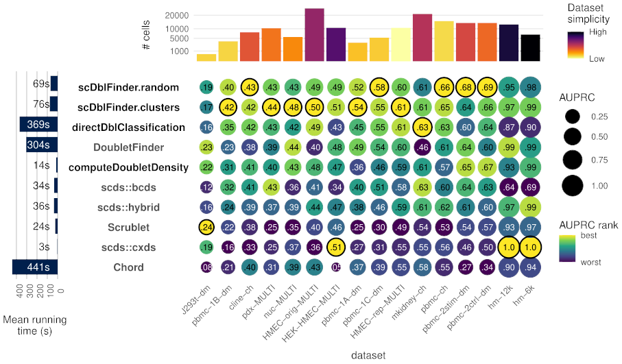 87 | **Figure1:** Accuracy (area under the precision and recall curve) of doublet identification using alternative methods across 16 benchmark datasets from Xi and Li (2020). The colour of the dots indicates the relative ranking for the dataset, while the size and numbers indicate the actual area under the (PR) curve. For each dataset, the top method is circled in black. Methods with names in black are provided in the `scDblFinder` package. Running times are indicated on the left. On top the number of cells in each dataset is shown, and colored by the proportion of variance explained by the first two components (relative to that explained by the first 100), as a rough guide to dataset simplicity.
88 |
89 |
90 |
87 | **Figure1:** Accuracy (area under the precision and recall curve) of doublet identification using alternative methods across 16 benchmark datasets from Xi and Li (2020). The colour of the dots indicates the relative ranking for the dataset, while the size and numbers indicate the actual area under the (PR) curve. For each dataset, the top method is circled in black. Methods with names in black are provided in the `scDblFinder` package. Running times are indicated on the left. On top the number of cells in each dataset is shown, and colored by the proportion of variance explained by the first two components (relative to that explained by the first 100), as a rough guide to dataset simplicity.
88 |
89 |
90 |
91 |
92 | Rather a python person? You can have a look at [vaeda](https://github.com/kostkalab/vaeda), another doublet finding method which appears to have performances close to those of scDblFinder. Alternatively, run scDblFinder [from the command line](https://plger.github.io/scDblFinder/articles/scDblFinder.html#how-can-i-call-scdblfinder-from-the-command-line).
93 |
--------------------------------------------------------------------------------
/vignettes/findDoubletClusters.Rmd:
--------------------------------------------------------------------------------
1 | ---
2 | title: Detecting clusters of doublet cells with DE analyses
3 | package: scDblFinder
4 | author:
5 | - name: Aaron Lun
6 | email: infinite.monkeys.with.keyboards@gmail.com
7 | date: "`r Sys.Date()`"
8 | output:
9 | BiocStyle::html_document
10 | vignette: |
11 | %\VignetteIndexEntry{3_findDoubletClusters}
12 | %\VignetteEngine{knitr::rmarkdown}
13 | %\VignetteEncoding{UTF-8}
14 | ---
15 |
16 | ```{r, echo=FALSE, message=FALSE}
17 | knitr::opts_chunk$set(error=FALSE, message=FALSE, warning=FALSE)
18 | library(BiocStyle)
19 | ```
20 |
21 | # tl;dr
22 |
23 | To demonstrate, we'll use one of the mammary gland datasets from the `r Biocpkg("scRNAseq")` package.
24 | We will subset it down to a random set of 500 cells for speed.
25 |
26 | ```{r}
27 | library(scRNAseq)
28 | sce <- BachMammaryData(samples="G_2")
29 |
30 | set.seed(1000)
31 | sce <- sce[,sample(ncol(sce), 500)]
32 | ```
33 |
34 | For the purposes of this demonstration, we'll perform an extremely expedited analysis.
35 | One would usually take more care here and do some quality control,
36 | create some diagnostic plots, etc., but we don't have the space for that.
37 |
38 | ```{r}
39 | library(scuttle)
40 | sce <- logNormCounts(sce)
41 |
42 | library(scran)
43 | dec <- modelGeneVar(sce)
44 |
45 | library(scater)
46 | set.seed(1000)
47 | sce <- runPCA(sce, ncomponents=10, subset_row=getTopHVGs(dec, n=1000))
48 |
49 | library(bluster)
50 | clusters <- clusterRows(reducedDim(sce, "PCA"), NNGraphParam())
51 |
52 | sce <- runTSNE(sce, dimred="PCA")
53 | plotTSNE(sce, colour_by=I(clusters), text_by=I(clusters))
54 | ```
55 |
56 | We then run `findDoubletClusters()` to test each cluster against the null hypothesis that it _does_ consist of doublets.
57 | The null is rejected if a cluster has many DE genes that lie outside the expression limits defined by the "source" clusters.
58 | On the other hand, if `num.de` is low, the cluster's expression profile is consistent with the doublet hypothesis.
59 |
60 | ```{r}
61 | library(scDblFinder)
62 | tab <- findDoubletClusters(sce, clusters)
63 | tab
64 | ```
65 |
66 | ```{r, echo=FALSE}
67 | # Sanity check that one of the clusters is a good doublet candidate.
68 | # If this fails, we probably need to pick a more demonstrative example.
69 | stopifnot(rownames(tab)[1]=="6")
70 | stopifnot(tab[1,"num.de"]==0)
71 | ```
72 |
73 | # Mathematical background
74 |
75 | Consider a cell population $i$ that has mean transcript count $\lambda_{gi}$ for gene $g$.
76 | Assume that each population exhibits a unique scaling bias $s_i$, representing the efficiency of library preparation for that population.
77 | The observed read/UMI count for each gene is then $\mu_{gi}=s_i\lambda_{gi}$.
78 | (For simplicity, we will ignore gene-specific scaling biases, as this is easily accommodated by considering $\lambda_{gi} \equiv \phi_g \lambda_{gi}$ for some bias $\phi_g$.)
79 | The expected total count for each population is $N_i = \sum_g \mu_{gi}$.
80 |
81 | Now, let us consider a doublet population $j$ that forms from two parent populations $i_1$ and $i_2$.
82 | The observed read count for $g$ in $j$ is $\mu_{gj} = s_j (\lambda_{gi_1} + \lambda_{gi_2})$.
83 | Note that $s_j$ need not be any particular function of $s_{i_1}$ and $s_{i_2}$.
84 | Rather, this relationship depends on how quickly the reverse transcription and amplification reagents are saturated during library preparation, which is difficult to make assumptions around.
85 |
86 | # Normalization by library size
87 |
88 | We obtain log-normalized expression values for each cell based on the library size.
89 | Assume that the library size-normalized expression values are such that $\mu_{gi_1}N_{i_1}^{-1} < \mu_{gi_2}N_{i_2}^{-1}$,
90 | i.e., the proportion of $g$ increases in $i_2$ compared to $i_1$.
91 | The contribution of each $s_i$ cancels out, yielding
92 | $$
93 | \frac{\lambda_{gi_1}}{\sum_g \lambda_{gi_1}} < \frac{\lambda_{gi_2}}{\sum_g \lambda_{gi_2}} \;.
94 | $$
95 | The normalized expression value of the doublet cluster $j$ is subsequently
96 | $$
97 | \frac{\lambda_{gi_1} + \lambda_{gi_2}}{\sum_g (\lambda_{gi_1} + \lambda_{gi_2})} \;,
98 | $$
99 | and it is fairly easy to show that
100 | $$
101 | \frac{\lambda_{gi_1}}{\sum_g \lambda_{gi_1}} <
102 | \frac{\lambda_{gi_1} + \lambda_{gi_2}}{\sum_g (\lambda_{gi_1} + \lambda_{gi_2})} <
103 | \frac{\lambda_{gi_2}}{\sum_g \lambda_{gi_2}} \;.
104 | $$
105 | In other words, the expected library size-normalized expression of our gene in the doublet cluster lies between that of the two parents.
106 |
107 | It is harder to provide theoretical guarantees with arbitrary size factors, which is why we only use the library sizes for normalization instead.
108 | The exception is that of spike-in size factors that would estimate $s_i$ directly.
109 | This would allow us to obtain estimates of $\lambda_{gi}$ for the parent clusters and of $\lambda_{gi_1} + \lambda_{gi_2}$ for the doublets.
110 | In this manner, we could more precisely identify doublet clusters as those where the normalized expression value is equal to the sum of the parents.
111 | Unfortunately, spike-ins are generally not available for droplet-based data sets where doublets are most problematic.
112 |
113 | # Testing for (lack of) intermediacy
114 |
115 | We want to identify the clusters that may be comprised of doublets of other clusters.
116 | For each cluster $j'$, we test for differential expression in the library size-normalized expression profiles against every other cluster $i'$.
117 | For each pair of other clusters $i'_1$ and $i'_2$, we identify genes that change in $j'$ against both $i'_1$ and $i'_2$ **in the same direction**.
118 | The presence of such genes violates the intermediacy expected of a doublet cluster and provides evidence that $j'$ is not a doublet of $i'_1$ and $i'_2$.
119 |
120 | Significant genes are identified by an intersection-union test on the $p$-values from the pairwise comparisons between $j'$ and $i'_1$ or $i'_2$.
121 | (Specifically, $t$-tests are used via the `findMarkers()` function from `r Biocpkg("scran")`.)
122 | The $p$-value for a gene is set to unity when the signs of the log-fold changes are not the same between comparisons.
123 | Multiple correction testing is applied using the Benjamini-Hochberg method, and the number of genes detected at a specified false discovery rate (usually 5\%) is counted.
124 | The pair $(i'_1, i'_2)$ with the fewest detected genes are considered as the putative parents of $j'$.
125 |
126 | In theory, it is possible to compute the Simes' combined $p$-value across all genes to reject the doublet hypothesis for $j'$.
127 | This would provide a more rigorous approach to ruling out potential doublet/parent combinations.
128 | However, this is very sensitive to misspecification of clusters -- see below.
129 |
130 | # Calling doublet clusters
131 |
132 | Assuming that most clusters are not comprised of doublets, we identify clusters that have an unusually low number of detected genes that violate the intermediacy condition.
133 | This is achieved by identifying small outliers on the log-transformed number of detected genes, using the median absolute deviation-based method in the \texttt{isOutlier} function.
134 | (We use a log-transformation simply to improve resolution at low values.)
135 | Clusters are likely to be doublets if they are outliers on this metric.
136 |
137 | Doublet clusters should also have larger library sizes than the proposed parent clusters.
138 | This is consistent with the presence of more RNA in each doublet, though the library size of the doublet cluster need not be a sum of that of the parent clusters
139 | (due to factors such as saturation and composition effects).
140 | The proportion of cells assigned to the doublet cluster should also be "reasonable";
141 | exactly what this means depends on the experimental setup and the doublet rate of the protocol in use.
142 |
143 | # Discussion
144 |
145 | The biggest advantage of this approach lies in its interpretability.
146 | Given a set of existing clusters, we can explicitly identify those that are likely to be doublets.
147 | We also gain some insight onto the parental origins of each putative doublet cluster, which may be of some interest.
148 | We avoid any assumptions about doublet formation that are otherwise necessary for the simulation-based methods.
149 | In particular, we do not require any knowledge about exact the relationship between $s_j$ and $s_i$, allowing us to identify doublets even when the exact location of the doublet is unknown (e.g., due to differences in RNA content between the parent clusters).
150 |
151 | The downside is that, of course, we are dependent on being supplied with sensible clusters where the parental and doublet cells are separated.
152 | The intermediacy requirement is loose enough to provide some robustness against misspecification, but this only goes so far.
153 | In addition, this strategy has a bias towards calling clusters with few cells as doublets (or parents of doublets) because the DE detection power is low.
154 | This can be somewhat offset by comparing `num.de` against `median.de` as latter will be low for clusters involved in systematically low-powered comparisons, though it is difficult to adjust for the exact effect of the differences of power on the IUT.
155 |
156 | # Session information {-}
157 |
158 | ```{r}
159 | sessionInfo()
160 | ```
161 |
--------------------------------------------------------------------------------
/vignettes/scATAC.Rmd:
--------------------------------------------------------------------------------
1 | ---
2 | title: "Doublet identifiation in single-cell ATAC-seq"
3 | author:
4 | - name: Pierre-Luc Germain
5 | affiliation: University and ETH Zürich
6 | package: scDblFinder
7 | output:
8 | BiocStyle::html_document
9 | abstract: |
10 | An introduction to the methods implemented for doublet detection in single-cell
11 | ATAC-seq.
12 | vignette: |
13 | %\VignetteIndexEntry{6_scATAC}
14 | %\VignetteEngine{knitr::rmarkdown}
15 | %\VignetteEncoding{UTF-8}
16 | ---
17 |
18 | ```{r, include=FALSE}
19 | library(BiocStyle)
20 | ```
21 |
22 | # Introduction
23 |
24 | Analyses in single-cell RNAseq are typically limited to a relatively small (e.g. one or two thousands) set of features that are most informative; these are often the genes with a higher expression (and hence more chances of being quantified).
25 | In contrast, single-cell ATACseq (scATACseq) data is considerably more sparse, with most reads being spread across hundreds of thousands of regions.
26 | In this context, selecting a subset of genes is highly ineffective, and therefore many of the methods developed for single-cell RNAseq are not easily applicable, and need to be adapted.
27 | Methods have therefore been developed specifically for scATACseq data (Granja et al. 2021; Thibodeau et al. 2021).
28 |
29 | This vignette presents different approaches to doublet detection in single-cell ATAC-seq implemented in the package: the first is an adaptation of `scDblFinder`, the second a reimplementation of the AMULET method from Thibodeau et al. (2021). The latter has the advantage of capturing homotypic doublets, but does not perform well in all datasets, and especially requires the cells to have a high library size. We therefore next present two ways of combining the two.
30 |
31 | # Applying the scDblFinder method
32 |
33 | With default parameters, the `scDblFinder` method performs very poorly on scATACseq data due to the increase spread of the reads across many features. Since working with all features (i.e. tiles or peaks) is computationally very expensive, an alternative approach is to begin by reducing the size of the dataset, not through _selection_ (as in scRNAseq), but by _aggregating_ correlated features into a relatively small set.
34 | This has the advantage of using all information, as well as making the count data more continuous.
35 | This method yields comparable performance to specialized single-cell ATACseq software (Germain et al., 2021).
36 |
37 | The feature aggregation can be triggered using the `aggregateFeatures=TRUE` argument, which will aggregate peak or tile counts into the number of meta-features defined by the `nfeatures`.
38 | If the number of meta-features is low (which we recommend), the meta-features can be directly used to calculated distances rather than going through the SVD step (which can be triggered with the `processing` argument). Such an example would be:
39 |
40 | ```{r}
41 | suppressPackageStartupMessages(library(scDblFinder))
42 | # we use a dummy SingleCellExperiment as example:
43 | sce <- mockDoubletSCE(ngenes=300)
44 | # setting low number of artificial doublets (same as ncells) just for speedup:
45 | sce <- scDblFinder(sce, artificialDoublets=1, aggregateFeatures=TRUE, nfeatures=25, processing="normFeatures")
46 | ```
47 |
48 | If you encounter problems running the aggregation-based approach on large datasets, first make sure you have the `mbkmeans` package installed.
49 |
50 | # Using the Amulet method
51 |
52 | The AMULET method from Thibodeau et al. (2021) is based on the assumption that, in a diploid cell, any given genomic region should be captured at most twice. Therefore, cells with loci covered by more than two fragments are indicative of the droplet being a doublet. Of note, this approach has the advantage of capturing homotypic doublets, which instead tend to be missed by other methods. Since it was only available in the form of a mixture of java and python scripts, we re-implemented the method in `scDblFinder` (see `?amulet`), leading to equal or superior results to the original implementation (Germain et al. 2021).
53 |
54 | As in the original implementation, we recommend excluding the mitochondrial and sex chromosomes, as well as repetitive regions. This can be specified with the `regionsToExclude` argument (see the underlying `?getFragmentOverlaps`). It can be used as follows:
55 |
56 | ```{r}
57 | # here we use a dummy fragment file for example:
58 | fragfile <- system.file("extdata", "example_fragments.tsv.gz", package="scDblFinder")
59 |
60 | # we might also give a GRanges of repeat elements, so that these regions are excluded:
61 | suppressPackageStartupMessages(library(GenomicRanges))
62 | repeats <- GRanges("chr6", IRanges(1000,2000))
63 | # it's better to combine these with mitochondrial and sex chromosomes
64 | otherChroms <- GRanges(c("M","chrM","MT","X","Y","chrX","chrY"),IRanges(1L,width=10^8))
65 | # here since I don't know what chromosome notation you'll be using I've just put them all,
66 | # although this will trigger a warning when combining them:
67 | toExclude <- suppressWarnings(c(repeats, otherChroms))
68 | # we then launch the method
69 | res <- amulet(fragfile, regionsToExclude=toExclude)
70 | res
71 | ```
72 |
73 | The results is a data.frame with statistics for each barcode, including a p-value. In contrast to the `scDblFinder` score, a lower p-value here is indicative of the droplet being more likely to be a doublet (as in the original method).
74 | By default, only the barcodes with a minimum number of reads are considered, but it is possible to specify the droplets for which to gather statistics using the `barcodes` argument.
75 |
76 | While the package includes an implementation that works based on peak/tile count matrices (see `?amuletFromCounts`), it has a much lower performance with respect to the one based directly on the fragment files (see `?amulet`), and we therefore discourage its use.
77 |
78 | The workhorse behind the `amulet` function is the `getFragmentOverlaps`, which also includes all of the relevant arguments.
79 | If the fragment files are not Tabix-indexed, the whole fragment file will have to be loaded in memory for processing; while this ensures relatively rapid computation, it has high memory requirements. Therefore, if the fragment file is Tabix-indexed (as is for instance done as part of the ArchR pipeline), it will be read and processed per chromosome, which is a little slower due to overhead, but keeps memory requirements rather low. This behavior can be disabled by specifying `fullInMemory=TRUE`.
80 |
81 | # Combining mehtods
82 |
83 | While the `scDblFinder`-based approach generally performs well, none of the two approach is optimal across all datasets tested. We therefore investigated two strategies for combining the rationales of each approach.
84 |
85 | The Amulet method tends to perform best with datasets that have homotypic doublets and where cells have a high library size (i.e. median library size per cell of 10-15k reads), while the `scDblFinder`-based approach works better for heterotypic doublets. Until an optimal solution is found, we recommend using multiple approaches to inform decisions, in particular using the p-value combination method below.
86 |
87 | ## The Clamulet method
88 |
89 | The `clamulet` method (Classification-powered Amulet-like method) operates similarly to the `scDblFinder` method, but generates artificial doublets by operating on the fragment coverages. This has the advantage that the number of loci covered by more than two reads can be computed for artificial doublets, enabling the use of this feature (along with the kNN-based ones) in a classification scheme. It however has the disadvantage of being rather slow and memory hungry, and appears to be outperformed by a simple p-value combination of the two methods (see below). We therefore _do not_ recommend its usage.
90 |
91 | The `clamulet` method uses the aforementioned aggregation approach, and its usage includes a number of arguments from both the `scDblFinder` and `amulet` method (see in particular `?getFragmentOverlaps`):
92 |
93 | ```{r, eval=FALSE}
94 | # not run
95 | d <- clamulet("path/to/fragments.tsv.gz")
96 | ```
97 |
98 | Since our dummy fragment file is so small (5 barcodes), here we'll have to adjust the arguments for an example to run:
99 |
100 | ```{r}
101 | d <- clamulet(fragfile, k=2, nfeatures=3)
102 | d
103 | ```
104 |
105 | The score can then be interpreted as for `scDblFinder`. We however note that this method proved *inferior to alternatives*.
106 |
107 | ## Simple p-value combination
108 |
109 | The amulet and scDblFinder scores above can be simply combined by treating them as p-values and aggregating them (here using Fisher's method from the `r CRANpkg("aggregation")` package, but see also the `r CRANpkg("metap")` package):
110 |
111 | ```{r, eval=FALSE}
112 | res$scDblFinder.p <- 1-colData(sce)[row.names(res), "scDblFinder.score"]
113 | res$combined <- apply(res[,c("scDblFinder.p", "p.value")], 1, FUN=function(x){
114 | x[x<0.001] <- 0.001 # prevent too much skew from very small or 0 p-values
115 | suppressWarnings(aggregation::fisher(x))
116 | })
117 | ```
118 |
119 | We found this to perform better than averaging the scores or their ranks, and while it is not the very best method in any of the datasets tested, it has a more robust performance overall (see Germain et al., 2021).
120 |
121 |
122 | # References
123 |
124 | Jeffrey M. Granja et al., “ArchR Is a Scalable Software Package for Integrative Single-Cell Chromatin Accessibility Analysis,” Nature Genetics, February 25, 2021, 1–9, https://doi.org/10.1038/s41588-021-00790-6
125 |
126 | Asa Thibodeau et al., “AMULET: A Novel Read Count-Based Method for Effective Multiplet Detection from Single Nucleus ATAC-Seq Data,” Genome Biology 22, no. 1 (December 2021): 252, https://doi.org/10.1186/s13059-021-02469-x
127 |
128 | Pierre-Luc Germain et al., “Doublet Identification in Single-Cell Sequencing Data Using ScDblFinder” (F1000Research, September 28, 2021), https://doi.org/10.12688/f1000research.73600.1
129 |
130 | # Session information {-}
131 |
132 | ```{r}
133 | sessionInfo()
134 | ```
135 |
--------------------------------------------------------------------------------
/R/getFragmentOverlaps.R:
--------------------------------------------------------------------------------
1 | #' getFragmentOverlaps
2 | #'
3 | #' Count the number of overlapping fragments.
4 | #'
5 | #' @param x The path to a fragments file, or a GRanges object containing the
6 | #' fragments (with the `name` column containing the barcode, and optionally
7 | #' the `score` column containing the count).
8 | #' @param barcodes Optional character vector of cell barcodes to consider
9 | #' @param minFrags Minimum number of fragments for a barcode to be
10 | #' considered. If `uniqueFrags=TRUE`, this is the minimum number of unique
11 | #' fragments. Ignored if `barcodes` is given.
12 | #' @param regionsToExclude A GRanges of regions to exclude. As per the original
13 | #' Amulet method, we recommend excluding repeats, as well as sex and
14 | #' mitochondrial chromosomes. (Note that the end coordinate does not need to
15 | #' be exact when excluding entire chromosomes, but greater or equal to the
16 | #' chromosome length.)
17 | #' @param uniqueFrags Logical; whether to use only unique fragments.
18 | #' @param maxFragSize Integer indicating the maximum fragment size to consider
19 | #' @param removeHighOverlapSites Logical; whether to remove sites that have
20 | #' more than two reads in unexpectedly many cells.
21 | #' @param fullInMemory Logical; whether to process all chromosomes together.
22 | #' This will speed up the process but at the cost of a very high memory
23 | #' consumption (as all fragments will be loaded in memory). This is anyway the
24 | #' default mode when `x` is not Tabix-indexed.
25 | #' @param verbose Logical; whether to print progress messages.
26 | #' @param BPPARAM A `BiocParallel` parameter object for multithreading. Note
27 | #' that multithreading will increase the memory usage.
28 | #' @param ret What to return, either barcode 'stats' (default), 'loci', or
29 | #' 'coverages'.
30 | #'
31 | #' @details When used on normal (or compressed) fragment files, this
32 | #' implementation is relatively fast (except for reading in the data) but it
33 | #' has a large memory footprint since the overlaps are performed in memory. It
34 | #' is therefore recommended to compress the fragment files using bgzip and index
35 | #' them with Tabix; in this case each chromosome will be read and processed
36 | #' separately, leading to a considerably lower memory footprint.
37 | #'
38 | #' @return A data.frame with counts and overlap statistics for each barcode.
39 | #'
40 | #' @importFrom GenomicRanges reduce GRanges granges GRangesList
41 | #' @importFrom BiocGenerics score
42 | #' @importFrom S4Vectors mcols
43 | #' @importFrom IRanges overlapsAny IRanges coverage slice
44 | #' @importFrom Rsamtools TabixFile seqnamesTabix
45 | #' @importFrom rtracklayer import
46 | #' @importFrom stats ppois
47 | #' @importFrom GenomeInfoDb keepSeqlevels seqlevels seqlevelsInUse
48 | #' @importFrom GenomeInfoDb seqlengths seqlengths<-
49 | #' @export
50 | getFragmentOverlaps <- function(x, barcodes=NULL, regionsToExclude=GRanges(
51 | c("M","chrM","MT","X","Y","chrX","chrY"),
52 | IRanges(1L,width=10^8)),
53 | minFrags=500L, uniqueFrags=TRUE,
54 | maxFragSize=1000L, removeHighOverlapSites=TRUE,
55 | fullInMemory=FALSE, BPPARAM=NULL, verbose=TRUE,
56 | ret=c("stats", "loci", "coverages")){
57 | # prepare inputs
58 | ret <- match.arg(ret)
59 | if(ret=="coverages" && !fullInMemory)
60 | stop("Returning coverages is currently only supported with fullInMemory=TRUE")
61 | if(is.null(BPPARAM)) BPPARAM <- BiocParallel::SerialParam()
62 | stopifnot(is.null(barcodes) || is.character(barcodes))
63 | if(!is.null(barcodes) && length(barcodes)==1 && file.exists(barcodes))
64 | barcodes <- readLines(barcodes) # assume barcodes to be a text file
65 | if(!is.null(regionsToExclude)){
66 | if(is.character(regionsToExclude) && length(regionsToExclude)==1 &&
67 | file.exists(regionsToExclude)){
68 | if(verbose) message(format(Sys.time(), "%X"),
69 | " - Reading regions to exclude")
70 | regionsToExclude <- rtracklayer::import(regionsToExclude)
71 | }else{
72 | stopifnot(is.null(regionsToExclude) || is(regionsToExclude, "GRanges"))
73 | }
74 | regionsToExclude <- sort(regionsToExclude)
75 | }
76 | # prepare empty output for returns
77 | emptyOutput <- data.frame(row.names=character(0), nFrags=integer(0),
78 | uniqFrags=integer(0), nAbove2=integer(0))
79 |
80 | if(is.character(x) && length(x)==1){
81 | if(!file.exists(x)) stop("x should be a fragment file!")
82 | if(!fullInMemory &&
83 | is(tf <- tryCatch(TabixFile(x), error=function(e) NULL), "TabixFile")){
84 | if(verbose) message(format(Sys.time(), "%X"),
85 | " - Reading Tabix-indexed fragment file and ",
86 | "computing overlaps")
87 | x <- bplapply(seqnamesTabix(tf), BPPARAM=BPPARAM, FUN=function(x){
88 | if(verbose) cat(paste0(x,", "))
89 | getFragmentOverlaps(
90 | rtracklayer::import(tf, format="bed",
91 | which=GRanges(x, IRanges(1,10^8))),
92 | barcodes, regionsToExclude=regionsToExclude, verbose=FALSE,
93 | minFrags=0.00001, uniqueFrags=uniqueFrags, maxFragSize=maxFragSize,
94 | removeHighOverlapSites=removeHighOverlapSites, BPPARAM=NULL, ret=ret
95 | )
96 | })
97 | if(verbose){
98 | cat("\n")
99 | message(format(Sys.time(), "%X"), " - Merging")
100 | }
101 | if(ret=="loci") return(unlist(GRangesList(x)))
102 | if(ret=="coverages"){
103 | return(x[[1]])
104 | # x <- lapply(x, as.list)
105 | # names(x) <- NULL
106 | # x <- lapply(x, FUN=function(x){
107 | # x[!sapply(x, FUN=function(x) length(x@values)==1L && all(x@values==0L))]
108 | # })
109 | # x <- x[lengths(x)>0L]
110 | # return(do.call(RleList, unlist(x, recursive=FALSE)))
111 | }
112 | x <- x[unlist(lapply(x,nrow))>0]
113 | if(length(x)==0) return(emptyOutput)
114 |
115 | if(is.null(barcodes)){
116 | barcodes <- rowsum(
117 | unlist(lapply(x, FUN=function(x) x$nFrags)),
118 | unlist(lapply(x, row.names)))[,1]
119 | barcodes <- names(barcodes[barcodes>=minFrags])
120 | }
121 | return(as.data.frame(Reduce("+", lapply(x, FUN=function(x){
122 | x <- as.matrix(x[barcodes,])
123 | x[is.na(x)] <- 0
124 | x
125 | })), row.names=barcodes))
126 | }else{
127 | if(!fullInMemory){
128 | message("Fragment file is not tabix-indexed, requiring the",
129 | "whole file to be imported in memory.")
130 | }else if(verbose){
131 | message(format(Sys.time(), "%X"), " - Reading full fragments...")
132 | }
133 | gr <- rtracklayer::import(x, format="bed")
134 | }
135 | }else{
136 | if(!is(x, "GRanges") || !("name" %in% colnames(mcols(x))))
137 | stop("`x` should either be a path to a fragments file, or a GRanges ",
138 | "with the 'name' column containing the cell barcode (and optionally
139 | the 'score' column containing the counts).")
140 | gr <- x
141 | }
142 | if(!all(!is.na(seqlengths(gr))))
143 | seqlengths(gr) <- setNames(sapply(split(end(gr), seqnames(gr)), max)
144 | [seqlevels(gr)], seqlevels(gr))
145 | gr <- gr[(width(gr)<=maxFragSize),]
146 | gr$name <- as.factor(gr$name)
147 | if(!is.null(regionsToExclude)){
148 | regionsToExclude <- regionsToExclude[which(
149 | as.factor(seqnames(regionsToExclude)) %in% seqlevels(gr))]
150 | if(length(regionsToExclude)>0){
151 | regionsToExclude <- keepSeqlevels(regionsToExclude,
152 | value=seqlevelsInUse(regionsToExclude),
153 | pruning.mode="coarse")
154 | seqlengths(regionsToExclude) <- NA
155 | gr <- gr[!overlapsAny(gr, regionsToExclude)]
156 | }
157 | }
158 |
159 | if(verbose) message(format(Sys.time(), "%X"),
160 | " - Splitting and subsetting barcodes...")
161 | uniqFrags <- table(gr$name)
162 | if(minFrags<1L & minFrags>0L) minFrags <- round(minFrags*length(gr))
163 | if(is.null(barcodes)){
164 | uniqFrags <- uniqFrags[uniqFrags>=minFrags]
165 | }else{
166 | if((mis <- length(setdiff(barcodes, names(uniqFrags))))>0)
167 | if(verbose)
168 | warning("Some barcodes (", mis, " or ",round(100*mis/length(gr),1),"%)",
169 | " are missing from the fragments file!")
170 | uniqFrags <- uniqFrags[intersect(names(uniqFrags), barcodes)]
171 | }
172 | gr <- gr[gr$name %in% names(uniqFrags)]
173 | gr$name <- droplevels(gr$name)
174 | if(length(gr)==0) return(emptyOutput)
175 | if(isFALSE(uniqueFrags) && !is.null(score(gr))){
176 | i <- rep(seq_along(gr), as.integer(score(gr)))
177 | gr <- GenomicRanges::split(granges(gr)[i], gr$name[i])
178 | rm(i)
179 | }else{
180 | gr <- GenomicRanges::split(granges(gr), gr$name)
181 | }
182 | if(ret=="coverages"){
183 | if(verbose) message(format(Sys.time(), "%X"), " - Computing coverages")
184 | return(lapply(gr, FUN=coverage))
185 | }
186 | if(verbose) message(format(Sys.time(), "%X"), " - Obtaining overlaps...")
187 | d <- data.frame(row.names=names(gr), nFrags=as.integer(lengths(gr)),
188 | uniqFrags=as.integer(uniqFrags[names(gr)]))
189 | d$nAbove2 <- 0L
190 | # obtain loci covered with >2 reads:
191 | grl <- GRangesList(lapply(gr, FUN=function(x){
192 | x <- slice(coverage(x), lower=3L, rangesOnly=TRUE)
193 | GRanges(rep(factor(names(x), seqlevels(gr)), lengths(x)),
194 | unlist(x, use.names=FALSE))
195 | }))
196 | gr2 <- unlist(grl, use.names=FALSE)
197 | gr2$name <- rep(factor(names(grl), row.names(d)),lengths(grl))
198 | if(ret=="loci") return(gr2)
199 | rm(grl,gr)
200 | gc(FALSE)
201 | tt <- table(gr2$name)
202 | d[names(tt),"total.nAbove2"] <- as.integer(tt)
203 | if(removeHighOverlapSites) gr2 <- .removeHighOverlapSites(gr2)
204 | tt <- table(gr2$name)
205 | d[names(tt),"nAbove2"] <- as.integer(tt)
206 | d
207 | }
208 |
209 | .removeHighOverlapSites <- function(gr, pthres=0.01, retExclusionRanges=FALSE){
210 | # remove loci that have >2 reads in too many cells
211 | ho <- reduce(gr, min.gapwidth=0L, with.revmap=TRUE)
212 | hol <- lengths(ho$revmap)
213 | ho$p <- ppois(hol, mean(hol), lower.tail=FALSE)
214 | if(length(indices2remove <- unlist(ho$revmap[which(ho$p<0.01)]))>0)
215 | gr <- gr[-indices2remove]
216 | if(retExclusionRanges) return(list(gr=gr, exclusion=granges(ho)))
217 | gr
218 | }
219 |
--------------------------------------------------------------------------------
/R/computeDoubletDensity.R:
--------------------------------------------------------------------------------
1 | #' Compute the density of simulated doublets
2 | #'
3 | #' Identify potential doublet cells based on the local density of simulated doublet expression profiles.
4 | #' This replaces the older \code{doubletCells} function from the \pkg{scran} package.
5 | #'
6 | #' @param x A numeric matrix-like object of count values,
7 | #' where each column corresponds to a cell and each row corresponds to an endogenous gene.
8 | #'
9 | #' Alternatively, a \linkS4class{SummarizedExperiment} or \linkS4class{SingleCellExperiment} object containing such a matrix.
10 | #' @param size.factors.norm A numeric vector of size factors for normalization of \code{x} prior to PCA and distance calculations.
11 | #' If \code{NULL}, defaults to size factors derived from the library sizes of \code{x}.
12 | #'
13 | #' For the SingleCellExperiment method, the default values are taken from \code{\link{sizeFactors}(x)}, if they are available.
14 | #' @param size.factors.content A numeric vector of size factors for RNA content normalization of \code{x} prior to simulating doublets.
15 | #' This is orthogonal to the values in \code{size.factors.norm}, see Details.
16 | #' @param k An integer scalar specifying the number of nearest neighbours to use to determine the bandwidth for density calculations.
17 | #' @param subset.row See \code{?"\link{scran-gene-selection}"}.
18 | #' @param niters An integer scalar specifying how many simulated doublets should be generated.
19 | #' @param block An integer scalar controlling the rate of doublet generation, to keep memory usage low.
20 | #' @param dims An integer scalar specifying the number of components to retain after the PCA.
21 | #' @param BNPARAM A \linkS4class{BiocNeighborParam} object specifying the nearest neighbor algorithm.
22 | #' This should be an algorithm supported by \code{\link{queryNeighbors}}.
23 | #' @param BSPARAM A \linkS4class{BiocSingularParam} object specifying the algorithm to use for PCA, if \code{d} is not \code{NA}.
24 | #' @param BPPARAM A \linkS4class{BiocParallelParam} object specifying whether the neighbour searches should be parallelized.
25 | #' @param ... For the generic, additional arguments to pass to specific methods.
26 | #'
27 | #' For the SummarizedExperiment and SingleCellExperiment methods, additional arguments to pass to the ANY method.
28 | #' @param assay.type A string specifying which assay values contain the count matrix.
29 | #'
30 | #' @return
31 | #' A numeric vector of doublet scores for each cell in \code{x}.
32 | #'
33 | #' @details
34 | #' This function simulates doublets by adding the count vectors for two randomly chosen cells in \code{x}.
35 | #' For each original cell, we compute the density of neighboring simulated doublets and compare it to the density of neighboring original cells.
36 | #' Genuine doublets should have a high density of simulated doublets relative to the density of its neighbourhood.
37 | #' Thus, the doublet score for each cell is defined as the ratio of densities of simulated doublets to the density of the original cells.
38 | #'
39 | #' Densities are calculated in low-dimensional space after a PCA on the log-normalized expression matrix of \code{x}.
40 | #' Simulated doublets are projected into the low-dimensional space using the rotation vectors computed from the original cells.
41 | #' For each cell, the density of simulated doublets is computed for a hypersphere with radius set to the median distance to the \code{k} nearest neighbour.
42 | #' This is normalized by \code{niters}, \code{k} and the total number of cells in \code{x} to yield the final score.
43 | #'
44 | #' The two size factor arguments have different roles:
45 | #' \itemize{
46 | #' \item \code{size.factors.norm} contains the size factors to be used for normalization prior to PCA and distance calculations.
47 | #' This defaults to the values returned by \code{\link{librarySizeFactors}} but can be explicitly set to ensure that the low-dimensional space is consistent with that in the rest of the analysis.
48 | #' \item \code{size.factors.content} is much more important, and represents the size factors that preserve RNA content differences.
49 | #' This is usually computed from spike-in RNA and ensures that the simulated doublets have the correct ratio of contributions from the original cells.
50 | #' }
51 | #' It is possible to set both of these arguments as they are orthogonal to each other.
52 | #' Setting \code{size.factors.content} will not affect the calculation of log-normalized expression values from \code{x}.
53 | #' Conversely, setting \code{size.factors.norm} will not affect the ratio in which cells are added together when simulating doublets.
54 | #'
55 | #' @author
56 | #' Aaron Lun
57 | #'
58 | #' @examples
59 | #' # Mocking up an example.
60 | #' set.seed(100)
61 | #' ngenes <- 1000
62 | #' mu1 <- 2^rnorm(ngenes)
63 | #' mu2 <- 2^rnorm(ngenes)
64 | #' mu3 <- 2^rnorm(ngenes)
65 | #' mu4 <- 2^rnorm(ngenes)
66 | #'
67 | #' counts.1 <- matrix(rpois(ngenes*100, mu1), nrow=ngenes) # Pure type 1
68 | #' counts.2 <- matrix(rpois(ngenes*100, mu2), nrow=ngenes) # Pure type 2
69 | #' counts.3 <- matrix(rpois(ngenes*100, mu3), nrow=ngenes) # Pure type 3
70 | #' counts.4 <- matrix(rpois(ngenes*100, mu4), nrow=ngenes) # Pure type 4
71 | #' counts.m <- matrix(rpois(ngenes*20, mu1+mu2), nrow=ngenes) # Doublets (1 & 2)
72 | #'
73 | #' counts <- cbind(counts.1, counts.2, counts.3, counts.4, counts.m)
74 | #' clusters <- rep(1:5, c(rep(100, 4), ncol(counts.m)))
75 | #'
76 | #' # Find potential doublets.
77 | #' scores <- computeDoubletDensity(counts)
78 | #' boxplot(split(log10(scores), clusters))
79 | #'
80 | #' @references
81 | #' Lun ATL (2018).
82 | #' Detecting doublet cells with \emph{scran}.
83 | #' \url{https://ltla.github.io/SingleCellThoughts/software/doublet_detection/bycell.html}
84 | #'
85 | #' @seealso
86 | #' \code{\link{findDoubletClusters}}, to detect doublet clusters.
87 | #'
88 | #' \code{\link{scDblFinder}}, which uses a hybrid approach involving simulation and overclustering.
89 | #'
90 | #' More detail on the mathematical background of this function is provided in the corresponding vignette at
91 | #' \code{vignette("computeDoubletDensity", package="scDblFinder")}.
92 | #'
93 | #' @name computeDoubletDensity
94 | NULL
95 |
96 | #' @importFrom scuttle librarySizeFactors normalizeCounts .bpNotSharedOrUp
97 | #' @importFrom SingleCellExperiment SingleCellExperiment logcounts
98 | #' @importFrom BiocParallel SerialParam bpmapply bpstart bpstop
99 | #' @importFrom Matrix rowMeans
100 | #' @importFrom stats median
101 | #' @importFrom BiocNeighbors findKNN findDistance queryNeighbors
102 | #' @importFrom BiocSingular runPCA bsparam
103 | #' @importFrom methods is
104 | #' @importFrom DelayedArray getAutoBPPARAM setAutoBPPARAM
105 | .doublet_cells <- function(x, size.factors.norm=NULL, size.factors.content=NULL,
106 | k=50, subset.row=NULL, niters=max(10000, ncol(x)), block=10000, dims=25,
107 | BNPARAM=KmknnParam(), BSPARAM=bsparam(), BPPARAM=SerialParam())
108 | {
109 | # Setting up the parallelization.
110 | old <- getAutoBPPARAM()
111 | setAutoBPPARAM(BPPARAM)
112 | on.exit(setAutoBPPARAM(old))
113 |
114 | if (.bpNotSharedOrUp(BPPARAM)){
115 | bpstart(BPPARAM)
116 | on.exit(bpstop(BPPARAM))
117 | }
118 |
119 | if (!is.null(subset.row)) {
120 | x <- x[subset.row,,drop=FALSE]
121 | }
122 | if (is.null(size.factors.norm)) {
123 | size.factors.norm <- librarySizeFactors(x, BPPARAM=BPPARAM)
124 | }
125 | if(!all(size.factors.norm>0))
126 | stop("Some size.factors are not positive. This typically happens ",
127 | "because some cells have no reads in the features specified by ",
128 | "`subset.row` -- these should be filtered out.")
129 |
130 | # Manually controlling the size factor centering here to ensure the final counts are on the same scale.
131 | size.factors.norm <- size.factors.norm/mean(size.factors.norm)
132 | if (!is.null(size.factors.content)) {
133 | x <- normalizeCounts(x, size.factors.content, log=FALSE, center_size_factors=FALSE)
134 | size.factors.norm <- size.factors.norm/size.factors.content
135 | }
136 | y <- normalizeCounts(x, size.factors.norm, center_size_factors=FALSE)
137 |
138 | # Running the PCA.
139 | pc.out <- runPCA(t(y), center=TRUE, BSPARAM=BSPARAM, rank=dims, BPPARAM=BPPARAM)
140 | pcs <- as.matrix(pc.out$x)
141 | sim.pcs <- .spawn_doublet_pcs(x, size.factors.norm, V=pc.out$rotation, centers=rowMeans(y), niters=niters, block=block)
142 |
143 | # Computing densities, using a distance computed from the kth nearest neighbor.
144 | self.dist <- findDistance(pcs, k=k, BNPARAM=BNPARAM, BPPARAM=BPPARAM)
145 | if(any(self.dist == 0))
146 | stop("Duplicate cells detected. These are probably low-quality cells ",
147 | "that have very few reads, and should be filtered out.")
148 |
149 | sim.n <- queryNeighbors(as.matrix(sim.pcs), query=pcs,
150 | threshold=self.dist * 1.00000001, # bump it up to avoid issues with numerical precision during tests.
151 | BNPARAM=BNPARAM, BPPARAM=BPPARAM,
152 | get.distance=FALSE, get.index=FALSE)
153 |
154 | sim.prop <- sim.n/niters
155 | sim.prop/(k/ncol(x))
156 | }
157 |
158 | #' @importFrom Matrix crossprod
159 | #' @importFrom scuttle normalizeCounts
160 | #' @importFrom DelayedArray sweep
161 | .spawn_doublet_pcs <- function(x, size.factors, V, centers, niters=10000L, block=10000L) {
162 | collected <- list()
163 | counter <- 1L
164 | current <- 0L
165 | mean.correction <- colSums(centers * V)
166 |
167 | while (current < niters) {
168 | to.make <- min(block, niters - current)
169 | left <- sample(ncol(x), to.make, replace=TRUE)
170 | right <- sample(ncol(x), to.make, replace=TRUE)
171 | sim.x <- x[,left,drop=FALSE] + x[,right,drop=FALSE]
172 |
173 | # Do not center, otherwise the simulated doublets will always have higher normalized counts
174 | # than actual doublets (as the latter will have been normalized to the level of singlets).
175 | sim.sf <- size.factors[left] + size.factors[right]
176 | sim.y <- normalizeCounts(sim.x, sim.sf, center_size_factors=FALSE)
177 |
178 | # Projecting onto the PC space of the original data.
179 | sim.pcs <- crossprod(sim.y, V)
180 | sim.pcs <- sweep(sim.pcs, 2L, mean.correction, FUN="-", check.margin=FALSE)
181 | collected[[counter]] <- sim.pcs
182 | counter <- counter + 1L
183 | current <- current + block
184 | }
185 |
186 | do.call(rbind, collected)
187 | }
188 |
189 | ##############################
190 | # S4 method definitions here #
191 | ##############################
192 |
193 | #' @export
194 | #' @rdname computeDoubletDensity
195 | setGeneric("computeDoubletDensity", function(x, ...) standardGeneric("computeDoubletDensity"))
196 |
197 | #' @export
198 | #' @rdname computeDoubletDensity
199 | setMethod("computeDoubletDensity", "ANY", .doublet_cells)
200 |
201 | #' @export
202 | #' @rdname computeDoubletDensity
203 | #' @importFrom SummarizedExperiment assay
204 | setMethod("computeDoubletDensity", "SummarizedExperiment", function(x, ..., assay.type="counts")
205 | {
206 | .doublet_cells(assay(x, i=assay.type), ...)
207 | })
208 |
209 | #' @export
210 | #' @rdname computeDoubletDensity
211 | #' @importFrom SummarizedExperiment assay
212 | #' @importFrom BiocGenerics sizeFactors
213 | setMethod("computeDoubletDensity", "SingleCellExperiment", function(x, size.factors.norm=sizeFactors(x), ...) {
214 | callNextMethod(x=x, size.factors.norm=size.factors.norm, ...)
215 | })
216 |
--------------------------------------------------------------------------------
/R/findDoubletClusters.R:
--------------------------------------------------------------------------------
1 | #' Detect doublet clusters
2 | #'
3 | #' Identify potential clusters of doublet cells based on whether they have intermediate expression profiles,
4 | #' i.e., their profiles lie between two other \dQuote{source} clusters.
5 | #'
6 | #' @param x A numeric matrix-like object of count values,
7 | #' where each column corresponds to a cell and each row corresponds to an endogenous gene.
8 | #'
9 | #' Alternatively, a \linkS4class{SummarizedExperiment} or \linkS4class{SingleCellExperiment} object containing such a matrix.
10 | #' @param clusters A vector of length equal to \code{ncol(x)}, containing cluster identities for all cells.
11 | #' If \code{x} is a SingleCellExperiment, this is taken from \code{\link{colLabels}(x)} by default.
12 | #' @param subset.row See \code{?"\link{scran-gene-selection}"}.
13 | #' @param threshold A numeric scalar specifying the FDR threshold with which to identify significant genes.
14 | #' @param ... For the generic, additional arguments to pass to specific methods.
15 | #'
16 | #' For the ANY method, additional arguments to pass to \code{\link{findMarkers}}.
17 | #'
18 | #' For the SummarizedExperiment method, additional arguments to pass to the ANY method.
19 | #'
20 | #' For the SingleCellExperiment method, additional arguments to pass to the SummarizedExperiment method.
21 | #' @param assay.type A string specifying which assay values to use, e.g., \code{"counts"} or \code{"logcounts"}.
22 | #' @param get.all.pairs Logical scalar indicating whether statistics for all possible source pairings should be returned.
23 | #'
24 | #' @return
25 | #' A \linkS4class{DataFrame} containing one row per query cluster with the following fields:
26 | #' \describe{
27 | #' \item{\code{source1}:}{String specifying the identity of the first source cluster.}
28 | #' \item{\code{source2}:}{String specifying the identity of the second source cluster.}
29 | #' \item{\code{num.de}:}{Integer, number of genes that are significantly non-intermediate
30 | #' in the query cluster compared to the two putative source clusters.}
31 | #' \item{\code{median.de}:}{Integer, median number of genes that are significantly non-intermediate
32 | #' in the query cluster across all possible source cluster pairings.}
33 | #' \item{\code{best}:}{String specifying the identify of the top gene with the lowest p-value
34 | #' against the doublet hypothesis for this combination of query and source clusters.}
35 | #' \item{\code{p.value}:}{Numeric, containing the adjusted p-value for the \code{best} gene.}
36 | #' \item{\code{lib.size1}:}{Numeric, ratio of the median library sizes for the first source cluster to the query cluster.}
37 | #' \item{\code{lib.size2}:}{Numeric, ratio of the median library sizes for the second source cluster to the query cluster.}
38 | #' \item{\code{prop}:}{Numeric, proportion of cells in the query cluster.}
39 | #' \item{\code{all.pairs}:}{A \linkS4class{SimpleList} object containing the above statistics
40 | #' for every pair of potential source clusters, if \code{get.all.pairs=TRUE}.}
41 | #' }
42 | #' Each row is named according to its query cluster.
43 | #'
44 | #' @details
45 | #' This function detects clusters of doublet cells in a manner similar to the method used by Bach et al. (2017).
46 | #' For each \dQuote{query} cluster, we examine all possible pairs of \dQuote{source} clusters,
47 | #' hypothesizing that the query consists of doublets formed from the two sources.
48 | #' If so, gene expression in the query cluster should be strictly intermediate
49 | #' between the two sources after library size normalization.
50 | #'
51 | #' We apply pairwise t-tests to the normalized log-expression profiles to reject this null hypothesis.
52 | #' This is done by identifying genes that are consistently up- or down-regulated in the query compared to \emph{both} sources.
53 | #' We count the number of genes that reject the null hypothesis at the specified FDR \code{threshold}.
54 | #' For each query cluster, the most likely pair of source clusters is that which minimizes the number of significant genes.
55 | #'
56 | #' Potential doublet clusters are identified using the following characteristics, in order of importance:
57 | #' \itemize{
58 | #' \item Low number of significant genes (i.e., \code{num.de}).
59 | #' Ideally, \code{median.de} is also high to indicate that the absence of strong DE is not due to a lack of power.
60 | #' \item A reasonable proportion of cells in the cluster, i.e., \code{prop}.
61 | #' This requires some expectation of the doublet rate in the experimental protocol.
62 | #' \item Library sizes of the source clusters that are below that of the query cluster, i.e., \code{lib.size*} values below unity.
63 | #' This assumes that the doublet cluster will contain more RNA and have more counts than either of the two source clusters.
64 | #' }
65 | #'
66 | #' For each query cluster, the function will only report the pair of source clusters with the lowest \code{num.de}.
67 | #' Setting \code{get.all.pairs=TRUE} will retrieve statistics for all pairs of potential source clusters.
68 | #' This can be helpful for diagnostics to identify relationships between specific clusters.
69 | #'
70 | #' The reported \code{p.value} is of little use in a statistical sense, and is only provided for inspection.
71 | #' Technically, it could be treated as the Simes combined p-value against the doublet hypothesis for the query cluster.
72 | #' However, this does not account for the multiple testing across all pairs of clusters for each chosen cluster,
73 | #' especially as we are chosing the pair that is most concordant with the doublet null hypothesis.
74 | #'
75 | #' We use library size normalization (via \code{\link{librarySizeFactors}}) even if existing size factors are present.
76 | #' This is because intermediate expression of the doublet cluster is not guaranteed for arbitrary size factors.
77 | #' For example, expression in the doublet cluster will be higher than that in the source clusters if normalization was performed with spike-in size factors.
78 | #'
79 | #' @author
80 | #' Aaron Lun
81 | #'
82 | #' @references
83 | #' Bach K, Pensa S, Grzelak M, Hadfield J, Adams DJ, Marioni JC and Khaled WT (2017).
84 | #' Differentiation dynamics of mammary epithelial cells revealed by single-cell RNA sequencing.
85 | #' \emph{Nat Commun.} 8, 1:2128.
86 | #'
87 | #' @seealso
88 | #' \code{\link{findMarkers}}, to detect DE genes between clusters.
89 | #'
90 | #' @examples
91 | #' # Mocking up an example.
92 | #' library(SingleCellExperiment)
93 | #' sce <- mockDoubletSCE(c(200,300,200))
94 | #'
95 | #' # Compute doublet-ness of each cluster:
96 | #' dbl <- findDoubletClusters(counts(sce), sce$cluster)
97 | #' dbl
98 | #'
99 | #' # Narrow this down to clusters with very low 'N':
100 | #' library(scuttle)
101 | #' isOutlier(dbl$num.de, log=TRUE, type="lower")
102 | #'
103 | #' # Get help from "lib.size" below 1.
104 | #' dbl$lib.size1 < 1 & dbl$lib.size2 < 1
105 | #'
106 | #' @name findDoubletClusters
107 | NULL
108 |
109 | #' @importFrom scuttle librarySizeFactors logNormCounts
110 | #' @importFrom scran findMarkers .logBH
111 | #' @importFrom BiocGenerics "sizeFactors<-" sizeFactors
112 | #' @importFrom stats p.adjust median
113 | #' @importFrom methods as
114 | #' @importClassesFrom S4Vectors SimpleList
115 | .doublet_cluster <- function(x, clusters, subset.row=NULL, threshold=0.05, get.all.pairs=FALSE, ...) {
116 | if (length(unique(clusters)) < 3L) {
117 | stop("need at least three clusters to detect doublet clusters")
118 | }
119 |
120 | # Computing normalized counts using the library size (looking for compositional differences!)
121 | sce <- SingleCellExperiment(list(counts=x))
122 | sizeFactors(sce) <- librarySizeFactors(x, subset_row=subset.row)
123 | sce <- logNormCounts(sce)
124 |
125 | degs <- findMarkers(sce, clusters, subset.row=subset.row, full.stats=TRUE, ...)
126 | med.lib.size <- vapply(split(sizeFactors(sce), clusters), FUN=median, FUN.VALUE=0)
127 | n.cluster <- table(clusters)/length(clusters)
128 |
129 | # Setting up the output.
130 | all.clusters <- names(degs)
131 | collected.top <- collected.all <- vector("list", length(all.clusters))
132 | names(collected.top) <- names(collected.all) <- all.clusters
133 |
134 | # Running through all pairs of clusters and testing against the third cluster.
135 | for (ref in all.clusters) {
136 | ref.stats <- degs[[ref]]
137 | remnants <- setdiff(all.clusters, ref)
138 |
139 | num <- length(remnants) * (length(remnants) - 1L)/2L
140 | all.N <- med.N <- all.gene <- all.parent1 <- all.parent2 <- integer(num)
141 | all.p <- numeric(num)
142 | idx <- 1L
143 |
144 | for (i1 in seq_along(remnants)) {
145 | stats1 <- ref.stats[[paste0("stats.", remnants[i1])]]
146 | for (i2 in seq_len(i1-1L)) {
147 | stats2 <- ref.stats[[paste0("stats.", remnants[i2])]]
148 |
149 | # Obtaining the IUT and setting opposing log-fold changes to 1.
150 | max.log.p <- pmax(stats1$log.p.value, stats2$log.p.value)
151 | max.log.p[sign(stats1$logFC) != sign(stats2$logFC)] <- 0
152 |
153 | # Correcting across genes. We use [1] to get NA when there are
154 | # no genes, which avoids an nrow() mismatch in DataFrame().
155 | log.adj.p <- .logBH(max.log.p)
156 | best.gene <- which.min(max.log.p)[1]
157 |
158 | all.N[idx] <- sum(log.adj.p <= log(threshold), na.rm=TRUE)
159 | all.gene[idx] <- best.gene
160 | all.p[idx] <- exp(log.adj.p[best.gene])
161 | all.parent1[idx] <- i1
162 | all.parent2[idx] <- i2
163 | idx <- idx + 1L
164 | }
165 | }
166 |
167 | # Formatting the output.
168 | parent1 <- remnants[all.parent1]
169 | parent2 <- remnants[all.parent2]
170 |
171 | stats <- DataFrame(source1=parent1, source2=parent2,
172 | num.de=all.N,
173 | median.de=rep(0, length(all.N)), # placeholder, see below.
174 | best=rownames(ref.stats)[all.gene],
175 | p.value=all.p,
176 | lib.size1=unname(med.lib.size[parent1]/med.lib.size[ref]),
177 | lib.size2=unname(med.lib.size[parent2]/med.lib.size[ref]))
178 |
179 | o <- order(all.N, -all.p)
180 | top <- cbind(stats[o[1],], prop=n.cluster[[ref]])
181 | med.de <- median(all.N)
182 | top$median.de <- med.de
183 | rownames(top) <- ref
184 | collected.top[[ref]] <- top
185 |
186 | if (get.all.pairs) {
187 | stats$median.de <- NULL
188 | collected.all[[ref]] <- stats[o,]
189 | }
190 | }
191 |
192 | # Returning the DataFrame of compiled results.
193 | out <- do.call(rbind, collected.top)
194 | if (get.all.pairs) {
195 | out$all.pairs <- as(collected.all, "SimpleList")
196 | }
197 | out[order(out$num.de),]
198 | }
199 |
200 | ##############################
201 | # S4 method definitions here #
202 | ##############################
203 |
204 | #' @export
205 | #' @rdname findDoubletClusters
206 | setGeneric("findDoubletClusters", function(x, ...) standardGeneric("findDoubletClusters"))
207 |
208 | #' @export
209 | #' @rdname findDoubletClusters
210 | setMethod("findDoubletClusters", "ANY", .doublet_cluster)
211 |
212 | #' @export
213 | #' @rdname findDoubletClusters
214 | #' @importFrom SummarizedExperiment assay
215 | setMethod("findDoubletClusters", "SummarizedExperiment", function(x, ..., assay.type="counts") {
216 | .doublet_cluster(assay(x, i=assay.type), ...)
217 | })
218 |
219 | #' @export
220 | #' @rdname findDoubletClusters
221 | #' @importFrom SingleCellExperiment colLabels
222 | setMethod("findDoubletClusters", "SingleCellExperiment", function(x, clusters=colLabels(x, onAbsence="error"), ...) {
223 | callNextMethod(x=x, clusters=clusters, ...)
224 | })
225 |
--------------------------------------------------------------------------------
/R/doubletThresholding.R:
--------------------------------------------------------------------------------
1 | #' doubletThresholding
2 | #'
3 | #' Sets the doublet scores threshold; typically called by
4 | #' \code{\link[scDblFinder]{scDblFinder}}.
5 | #'
6 | #' @param d A data.frame of cell properties, with each row representing a cell, as
7 | #' produced by `scDblFinder(..., returnType="table")`, or minimally containing a `score`
8 | #' column.
9 | #' @param dbr The expected (mean) doublet rate. If `d` contains a `cluster` column, the
10 | #' doublet rate will be adjusted for homotypic doublets.
11 | #' @param dbr.sd The standard deviation of the doublet rate, representing the
12 | #' uncertainty in the estimate. Ignored if `method!="optim"`.
13 | #' @param dbr.per1k The expected proportion of doublets per 1000 cells.
14 | #' @param stringency A numeric value >0 and <1 which controls the relative weight of false
15 | #' positives (i.e. real cells) and false negatives (artificial doublets) in setting the
16 | #' threshold. A value of 0.5 gives equal weight to both; a higher value (e.g. 0.7) gives
17 | #' higher weight to the false positives, and a lower to artificial doublets. Ignored if
18 | #' `method!="optim"`.
19 | #' @param method The thresholding method to use, either 'auto' (default, automatic
20 | #' selection depending on the available fields), 'optim' (optimization of
21 | #' misclassification rate and deviation from expected doublet rate), 'dbr' (strictly
22 | #' based on the expected doublet rate), or 'griffiths' (cluster-wise number of
23 | #' median absolute deviation in doublet score).
24 | #' @param perSample Logical; whether to perform thresholding individually for each sample.
25 | #' @param p The p-value threshold determining the deviation in doublet score.
26 | #' @param returnType The type of value to return, either doublet calls (`call`) or
27 | #' thresholds (`threshold`).
28 | #'
29 | #' @return A vector of doublet calls if `returnType=="call"`, or a threshold (or vector
30 | #' of thresholds) if `returnType=="threshold"`.
31 | #'
32 | #' @importFrom stats pcauchy optimize ecdf lm predict dnbinom quantile
33 | #'
34 | #' @examples
35 | #' sce <- mockDoubletSCE()
36 | #' d <- scDblFinder(sce, verbose=FALSE, returnType="table")
37 | #' th <- doubletThresholding(d, dbr=0.05)
38 | #' th
39 | #'
40 | #' @importFrom stats mad qnorm setNames
41 | #' @export
42 | doubletThresholding <- function( d, dbr=NULL, dbr.sd=NULL, dbr.per1k=0.008,
43 | stringency=0.5, p=0.1,
44 | method=c("auto","optim","dbr","griffiths"),
45 | perSample=TRUE, returnType=c("threshold","call")){
46 | method <- match.arg(method)
47 | returnType <- match.arg(returnType)
48 | if(is.null(d$src)) d$src <- d$type
49 | if(is.null(dbr.sd)) dbr.sd <- mean(0.4*.gdbr(d,dbr))
50 | dbr <- .estimateHeterotypicDbRate(d, .checkPropArg(dbr))
51 | if(!is.data.frame(d) && !is(d,"DFrame"))
52 | stop("`d` should be a data.frame with minimally the 'score' column.")
53 | conds <- list("optim"=c("type","score"),
54 | "dbr"=c("score"),
55 | "griffiths"=c("score"))
56 | w <- vapply(conds, FUN.VALUE=logical(1), FUN=function(x) all(x %in% colnames(d)))
57 | if(method=="auto"){
58 | if(length(w)==0) stop("`d` misses the necessary columns.")
59 | method <- names(conds)[which(w)[1]]
60 | }else{
61 | if(!w[[method]]) stop("`d` misses the necessary columns.")
62 | }
63 | if(method=="optim"){
64 | if(is.null(d$cluster)) d$cluster <- 1L
65 | if(!all(sort(as.character(unique(d$type)))==c("doublet","real")))
66 | stop("`type` should be either 'real' or 'doublet'.")
67 | if(is.null(d$include.in.training)) d$include.in.training <- TRUE
68 | if(!is.null(d$sample) && perSample){
69 | si <- split(seq_len(nrow(d)), d$sample)
70 | if(!is.null(dbr)){
71 | if(length(dbr)==1) dbr <- setNames(rep(dbr, length(si)), names(si))
72 | if(!all(names(si) %in% names(dbr)))
73 | stop("The names of `dbr` do not correspond to samples of `d`")
74 | }
75 | th <- sapply(setNames(names(si),names(si)), FUN=function(s){
76 | .optimThreshold(d[si[[s]],c("type","src","score","cluster","include.in.training")],
77 | dbr=dbr[[s]], dbr.sd=dbr.sd, stringency=stringency)
78 | })
79 | ret <- as.factor(d$score > th[d$sample])
80 | }else{
81 | th <- .optimThreshold(d, dbr=.gdbr(d,dbr), dbr.sd=dbr.sd, stringency=stringency)
82 | ret <- as.factor(d$score>th)
83 | }
84 | if(returnType=="threshold") return(th)
85 | }else{
86 | if(!is.null(d$src)) d <- d[d$src=="real",]
87 | if(method=="dbr"){
88 | th <- quantile(d$score, 1-dbr)
89 | if(returnType=="threshold") return(th)
90 | ret <- as.factor(d$score>th)
91 | }else if(method=="griffiths"){
92 | if(!("sample" %in% colnames(d))) d$sample <- "all"
93 | i <- split(seq_len(nrow(d)), d$sample)
94 | meds <- vapply(i, FUN.VALUE=numeric(1), FUN=function(x){
95 | median(d$score[x],na.rm=TRUE)
96 | })
97 | d$dev <- d$score-meds[d$sample]
98 | mad <- vapply(i, FUN.VALUE=numeric(1), FUN=function(x){
99 | x <- d$dev[x]
100 | median(x[x>0],na.rm=TRUE)
101 | }) * formals(mad)$constant
102 | if(returnType=="threshold"){
103 | return(qnorm(p, mean=meds, sd=mad, lower.tail=FALSE))
104 | }else{
105 | d$p <- pnorm(d$score, mean=meds[d$sample], sd=mad[d$sample],
106 | lower.tail=FALSE)
107 | ret <- as.factor(d$p < p)
108 | }
109 | }else{
110 | stop("Unknown method '",method,"'")
111 | }
112 | }
113 | levels(ret) <- c("singlet","doublet")
114 | return(ret)
115 | }
116 |
117 | # dbr should be already corrected for homotypy
118 | .optimThreshold <- function(d, dbr=NULL, dbr.sd=NULL, ths=NULL, stringency=0.5){
119 | if(!(stringency > 0) || !(stringency<1))
120 | stop("`stringency` should be >0 and <1.")
121 | if(is.null(dbr)) dbr <- .gdbr(d, dbr=.estimateHeterotypicDbRate(d))
122 | if(!is.null(dbr.sd)) dbr <- c(max(0,dbr-dbr.sd), min(1,dbr+dbr.sd))
123 | if(is.null(d$cluster)) d$cluster <- 1L
124 | wR <- which(d$src=="real")
125 | expected <- dbr*length(wR)
126 | if(!is.logical(d$type)) d$type <- d$type=="real"
127 | fdr.include <- which(d$include.in.training)
128 | eFN <- sum(grepl("^rDbl\\.",row.names(d))) *
129 | propHomotypic(d$cluster[d$src=="real"])
130 | if(length(unique(d$cluster))==1) eFN <- 0
131 | totfn <- function(x){
132 | edev <- .prop.dev(d$type,d$score,expected,x)^2
133 | y <- edev + 2*(1-stringency)*.FNR(d$type, d$score, x, expectedFN=eFN)
134 | if(!is.null(fdr.include))
135 | y <- y + .FPR(d$type[fdr.include], d$score[fdr.include], x)*2*stringency
136 | y
137 | }
138 | if(is.null(ths)) return(optimize(totfn, c(0,1), maximum=FALSE)$minimum)
139 | data.frame( threshold=ths,
140 | FNR=vapply(ths, FUN.VALUE=numeric(1), FUN=function(x){
141 | .FNR(d$type, d$score, x, expectedFN=eFN)
142 | }),
143 | FDR=vapply(ths, FUN.VALUE=numeric(1), FUN=function(x){
144 | .FDR(d$type[fdr.include], d$score[fdr.include], x)
145 | }),
146 | FPR=vapply(ths, FUN.VALUE=numeric(1), FUN=function(x){
147 | .FPR(d$type[fdr.include], d$score[fdr.include], x)
148 | }),
149 | dev=vapply(ths, FUN.VALUE=numeric(1), FUN=function(x){
150 | .prop.dev(d$type,d$score,expected,x)^2
151 | }),
152 | cost=vapply(ths, FUN.VALUE=numeric(1), FUN=totfn)
153 | )
154 | }
155 |
156 | .FNR <- function(type, score, threshold, expectedFN=0){
157 | if(!is.logical(type)) type <- type=="real"
158 | max(c(0, (sum(!type & score=threshold, na.rm=TRUE)==0) return(0)
162 | if(!is.logical(type)) type <- type=="real"
163 | sum(type & score>=threshold, na.rm=TRUE)/sum(score>=threshold, na.rm=TRUE)
164 | }
165 | .FPR <- function(type, score, threshold){
166 | if(length(type)==0) return(0)
167 | if(!is.logical(type)) type <- type=="real"
168 | sum(type & score>=threshold, na.rm=TRUE)/sum(type)
169 | }
170 |
171 | .prop.dev <- function(type, score, expected, threshold){
172 | if(!is.logical(type)) type <- type=="real"
173 | x <- 1+sum(score>=threshold & type)
174 | expected <- expected + 1
175 | if(length(expected)>1 && x>min(expected) && x=th]
207 | expected <- getExpectedDoublets(d$cluster[d$src=="real"], dbr=dbr)
208 | stats <- .compareToExpectedDoublets(o, dbr=dbr, expected=expected)
209 | stats$combination <- as.character(stats$combination)
210 | stats$FNR <- vapply(split(as.data.frame(d), d$mostLikelyOrigin),
211 | FUN.VALUE=numeric(1L),
212 | FUN=function(x) .FNR(x$type, x$score, th) )[stats$combination]
213 | stats$difficulty <- vapply(split(d$difficulty, d$mostLikelyOrigin),
214 | FUN.VALUE=numeric(1L), na.rm=TRUE,
215 | FUN=median)[stats$combination]
216 | stats
217 | }
218 |
219 | #' @importFrom stats quantile
220 | .filterUnrecognizableDoublets <- function( d, minSize=5, minMedDiff=0.1 ){
221 | if(is.null(d$src)) d$src <- d$type
222 | da <- d[d$src=="artificial" & grepl("+", d$mostLikelyOrigin, fixed=TRUE),]
223 | dr <- d[d$src=="real",]
224 | dr.med <- median(dr$score)
225 | dr <- split(dr$score, dr$cluster)
226 | rq <- t(vapply(dr, FUN.VALUE=numeric(2), na.rm=TRUE, probs=c(0.5, 0.9), FUN=quantile))
227 | da <- split(da$score, droplevels(da$mostLikelyOrigin))
228 | origs <- strsplit(names(da), "+", fixed=TRUE)
229 | out <- vapply(names(da), FUN.VALUE=logical(1), FUN=function(x){
230 | z <- da[[x]]
231 | if(length(z)