├── .gitattributes
├── CHANGELOG.md
├── LICENSE
├── README.md
├── THIRDPARTY
├── cfdtool.m
├── download.png
├── screenshot.jpg
└── tutorials
├── 01_Quickstart
├── 02_heat_exchanger1.fes
├── 03_axisymmetric_flow1.fes
├── 04_natural_convection1.fes
├── axisymmetric_flow1.jpg
├── heat_exchanger1.jpg
└── natural_convection1.jpg
├── 02_Heat_Transfer
├── 01_heat_transfer1.fes
├── 02_heat_transfer2.fes
├── 03_heat_transfer3.fes
├── 05_thermal_bridge1.fes
├── 07_heat_transfer5.fes
├── heat_transfer1.jpg
├── heat_transfer2.jpg
├── heat_transfer3.jpg
├── heat_transfer5.jpg
└── thermal_bridge1.jpg
├── 03_Fluid_Dynamics
├── 01_channel_flow1.fes
├── 02_driven_cavity1.fes
├── 03_flow_around_cylinder1.fes
├── 04_backwards_facing_step1.fes
├── 05_vortex_flow1.fes
├── 07_compressible_euler1.fes
├── 08_compressible_euler2.fes
├── 09_turbulent_channel1.fes
├── 10_turbulent_flow1.fes
├── 11_taylor_couette1.fes
├── 12_non_newtonian1.fes
├── 13_compressible_flow1.fes
├── backwards_facing_step1.jpg
├── channel_flow1.jpg
├── compressible_euler1.jpg
├── compressible_euler2.jpg
├── compressible_flow1.jpg
├── driven_cavity1.jpg
├── flow_around_cylinder1.jpg
├── non_newtonian1.jpg
├── taylor_couette1.jpg
├── turbulent_channel1.jpg
├── turbulent_flow1.jpg
└── vortex_flow1.jpg
└── webtutlist
/.gitattributes:
--------------------------------------------------------------------------------
1 | *.html linguist-detectable=false
2 | *.js linguist-detectable=false
3 | *.md linguist-detectable=false
4 | *.xml linguist-detectable=false
--------------------------------------------------------------------------------
/CHANGELOG.md:
--------------------------------------------------------------------------------
1 | CFDTool Changelog
2 | ===================
3 |
4 |
5 | 2025-02-14 version 1.10.3
6 | -------------------------
7 |
8 | - Warning for MATLAB 2025a GUI incompatibility and performance
9 | - Add checkbox toggle for flow mode automatic pressure contstraint
10 | - Warning for incompatible (openfoam.org foundation) OpenFOAM installation
11 | - Minor bug fixes
12 |
13 | 2024-11-27 version 1.10.2
14 | -------------------------
15 |
16 | - OpenFOAM/SU2 add option to save casefiles on error
17 | - GUI consistency improvements
18 | - SU2 default to V2003m SST turbulence model
19 | - Minor bug fixes
20 |
21 |
22 | 2024-10-20 version 1.10.1
23 | -------------------------
24 |
25 | - Added categories to physics mode selection list
26 | - Recommendation to use ESI openfoam.com (not openfoam.org)
27 | - Minor bug fixes
28 |
29 |
30 | 2024-09-30 version 1.10
31 | -----------------------
32 |
33 | - Unified UI with FEATool
34 | - Physics mode for compressible high Ma number turbulent flows
35 | + Add tutorial model for supersonic compressible flow past a prism
36 | - Updated OpenFOAM solver interface
37 | + Support coupled flow + heat transfer
38 | + Support for multiple subdomains
39 | + Support for chtMultiRegionFoam, buoyantBoussinesqFoam, and sonicFoam solvers
40 | + CFD script model support for the OpenFOAM solver
41 | - SU2 support for turbulent compressible and high Ma flows
42 | - Improved UI performance and responsiveness
43 |
44 |
45 | 2024-06-25 version 1.9.6
46 | ------------------------
47 |
48 | - MacOS App OpenFOAM support (https://github.com/gerlero/openfoam-app)
49 | - Removed averaging of initial conditions for boundaries shared between subdomains
50 | - Improved performance of Robin boundary condition assembly
51 | - Fix for 3D geometry plotting (identification and deduplication of shared boundaries)
52 |
53 |
54 | 2024-03-15 version 1.9.5
55 | ------------------------
56 |
57 | - Support CSG formulas for robust (STL/OBJ) meshes
58 | - New supersonic flow passed a wedge tutorial
59 | - Change supersonic flow over bump tutorial to 3D
60 | - Support HOME/Documents/MATLAB/.cfdtool/cfdtool.ini configuration
61 | + performance mex and mumps solver disabled by default
62 | - Fix bug in geometry object rotation
63 | - Minor fixes
64 |
65 |
66 | 2023-11-30 version 1.9.4
67 | ------------------------
68 |
69 | - Fix Excel (xlsx) data export
70 | - Add Data Export dialog box
71 | + Support custom data export expressions
72 | + Support custom data export coordinates
73 | - Improved app startup and shutdown time
74 |
75 |
76 | 2023-09-10 version 1.9.3
77 | ------------------------
78 |
79 | - Add equation mode menu option to remove physics modes
80 | - Updated OpenCASCADE geometry kernel to v7.7.2
81 | - Fix 2D STEP/IGES geometry import
82 | - Fix plot 3D block/hexahedal grid
83 | - Fix for Matlab 2023b
84 |
85 |
86 | 2023-03-12 version 1.9.2
87 | ------------------------
88 |
89 | - Show axes coordinate system orientation for 3D views
90 | - Update MUMPS linear solver
91 | + Support all MATLAB versions (Windows and Linux)
92 | + Support for Intel MKL BLAS, OpenMP, and >2GB large arrays
93 | - Updated SU2 Code CFD solver to v7.5.0
94 | - Add functionality to show geometry object information
95 |
96 |
97 | 2022-10-20 version 1.9.1
98 | ------------------------
99 |
100 | - Updated m-file export output to support the MATLAB "publish" command
101 | - New "Create Model Report" menu option to Generate model reports in
102 | Html, PDF, Microsoft Word/PDF, Latex, and XML formats
103 | - Updated OpenCASCADE geometry kernel to v7.6.3
104 | - Updated SU2 Code CFD solver to v7.4.0
105 |
106 |
107 | 2022-08-29 version 1.9
108 | -----------------------
109 |
110 | - Performance improvements for built-in multiphysics solver
111 | - Improved 3D geometry rendering performance
112 | - New 3D geometry defeaturing functionality
113 | - Support for edge/vertex selection for chamfer/fillet operations
114 | - Support for PDF image and Excel data export
115 | - Improved save/load model file performance
116 |
117 |
118 | 2022-06-06 version 1.8.5
119 | ------------------------
120 |
121 | - Fix for STEP geometry import with >= 2 objects
122 | - Improved and faster expression evaluation in assembly
123 |
124 |
125 | 2022-05-09 version 1.8.4
126 | -------------------------
127 |
128 | - Added 2D geometry tool for Bezier and spline curves
129 | - Updated OpenCASCADE geometry kernel to v7.6.2
130 | - Support for binary brep (.bin) geometry format
131 | - Updated SU2 Code CFD solver to v7.3.1
132 | - Added k-Omega wall function support for SU2 solver
133 |
134 |
135 | 2021-12-01 version 1.8.1
136 | -------------------------
137 | - Geometry import option from bitmap image (bmp, jpeg, png)
138 | - Support for structured meshing of geometry primitives
139 | - Updated plotly library to version 2.6.2
140 | - Updated ParaView Glance library to version 4.17.1,
141 | and added support for slice and isosurface plot options
142 | - Linux support for HiDPI screens
143 | - Mouse controls for 3D zoom, pan, and rotate
144 |
145 |
146 | 2021-11-01 version 1.8
147 | ----------------------
148 |
149 | - Improved graphics performance for 3D plots
150 | - Changed 3D plots to fill the whole viewport with
151 | CAD style orbit, pan, and zoom controls
152 | - Added flip/reverse view option by double clicking
153 | on the 3D xy, xz, and yz quickview buttons
154 |
155 |
156 | 2021-08-30 version 1.7.3
157 | ------------------------
158 |
159 | - Added view boundaries/subdomains menu option
160 | (for specifying mesh sizes on individual geometric entities)
161 | - Various performance improvements
162 |
163 |
164 | 2021-05-24 version 1.7.1
165 | ------------------------
166 |
167 | - Preliminary support for built-in and robust 3D mesh generators
168 | - GUI menu option to manually renumber/reassign 3D boundaries
169 | - Heated pipe with cooling fins validation tutorial
170 |
171 |
172 | 2020-04-19 version 1.7
173 | ----------------------
174 |
175 | - Minor update to sync with FEATool v1.14
176 |
177 |
178 | 2020-03-26 version 1.6
179 | ----------------------
180 |
181 | - Updated OpenFOAM and SU2 interfaces to support parallel computations
182 | - Added OpenFOAM binary GUI option to support user defined FOAM solvers
183 | - Added support for ESI-OpenCFD native Windows OpenFOAM distribution
184 |
185 |
186 | 2020-11-01 version 1.5
187 | ----------------------
188 |
189 | - Support 3D geometry and CAD modeling
190 | - SU2 external CFD solver integration
191 |
192 |
193 | 2019-09-01 version 1.4
194 | ----------------------
195 |
196 | - Support for .fes script file format
197 | - Added built in CFD tutorials
198 |
199 |
200 | 2018-11-20 version 1.3
201 | ----------------------
202 |
203 | - Support for supersonic and inviscid compressible flows
204 | (compressible Euler equations)
205 | - OpenFOAM support for inviscid compressible flows
206 | - Monitoring of OpenFOAM convergence curves
207 | - NACA 4-series pre-defined wing geometry object
208 |
209 |
210 | 2018-10-22 version 1.2
211 | ----------------------
212 |
213 | - OpenFOAM external CFD solver integration
214 | - Support for k-epsilon/omega turbulence models (with OpenFOAM)
215 | - Potential flow velocity field initialization
216 | - Improved resolution of curved geometry boundaries
217 |
218 |
219 | 2018-09-24 version 1.1
220 | ----------------------
221 |
222 | - Support for 2D Axisymmetry/Cylindrical coordinates
223 | and flows with swirl (non-zero azimuthal velocity)
224 | - Support for heat transfer modeling in 1D
225 | - Support for importing 2D planar STL CAD geometry files
226 | - Built-in interface to the external mesh generator
227 | Gridgen2D with support for meshing boundary layers
228 | - Support for importing Gmsh, GiD, Triangle, and FEniCS
229 | grid and mesh formats
230 | - Improved parametrization and meshing of curved boundaries
231 | - Added automatic shock capturing and stabilization for
232 | convection dominated flow regimes
233 | - Improved and more efficient flow discretization
234 | - Added advanced postprocessing functionality such as boundary
235 | integration for computation of drag and lift coefficients
236 | - Extended backwards compatibility to MATLAB 2009b
237 |
238 |
239 | 2018-08-05 version 1.0
240 | ----------------------
241 |
242 | - Initial release
243 |
--------------------------------------------------------------------------------
/LICENSE:
--------------------------------------------------------------------------------
1 | Precise Simulation Limited Software License Agreement
2 |
3 | CAREFULLY READ THE FOLLOWING TERMS AND CONDITIONS ("TERMS") BEFORE
4 | INSTALLING OR USING THE PROGRAMS OR DOCUMENTATION. INSTALLING OR USING
5 | THE PROGRAMS MEANS YOU HAVE ACCEPTED AND AGREE TO BE BOUND BY THE
6 | TERMS AND CONDITIONS OF THIS AGREEMENT. IF YOU DO NOT ACCEPT THEM,
7 | UNINSTALL, REMOVE AND COMPLETELY DELETE THE PROGRAMS AND
8 | DOCUMENTATION.
9 |
10 | 1. Preamble: This Agreement governs the relationship between the
11 | Licensee ("you", "your") and Licensor Precise Simulation Limited
12 | ("we", "us", "ours"). This Agreement sets the terms, rights,
13 | restrictions and obligations on using the FEATool and/or CFDTool
14 | ("Software", "Program(s)") and documentation ("Documentation")
15 | created and owned by Licensor, as detailed herein.
16 |
17 | 2. License Grant: Licensor hereby grants Licensee a Non-assignable &
18 | Non-transferable, Non-exclusive license to run and use the Program,
19 | without the rights to create derivative works, all with accordance
20 | with the terms set forth and other legal restrictions set forth in 3rd
21 | party software used while running Software.
22 |
23 | 2.1 Programs: You may license a specified single installation license
24 | ("SUL"), multi-user/floating network license ("MUL"), or ("CKL") class
25 | kit license under this Agreement, and your license rights are for the
26 | number of installations and users set forth on the purchase order,
27 | agreement, or issued invoice. A free limited and restricted license
28 | ("FREE/TRIAL") is granted for personal, non-commercial use for
29 | evaluation purposes.
30 |
31 | a. the FREE/TRIAL license option is restricted to personal, trial, and
32 | non-commercial use allowing for a single installation and concurrent
33 | use of the Program. You may NOT use the Program with a FREE/TRIAL
34 | license for any commercial, or production use, i.e., you may only use
35 | the Program for experimental, personal, and trial use (to test the
36 | Program). Specifically, the restrictions of the FREE/TRIAL license
37 | Program and Software may not be circumvented in any way without
38 | Payment for an upgraded license.
39 |
40 | b. the specified single installation license SUL must be installed on
41 | a specified computer system and its use is limited to a single
42 | concurrent instance. To change system a system transfer fee may be
43 | required.
44 |
45 | c. the multi-use license option MUL may be installed on a single
46 | networked system or server, or several systems and run concurrently
47 | the number of instances specified in the purchase order, agreement, or
48 | issued invoice.
49 |
50 | d. academic granting institutions with the class kit license CKL
51 | option may install and use the Software in a computer lab/systems
52 | belonging to the institute/institution and run concurrently the number
53 | of instances specified in the purchase order, agreement, or issued
54 | invoice.
55 |
56 | e. regardless of which license you have, you shall use the Programs
57 | only for your internal operations. For the purposes of this Agreement,
58 | "internal operations" means use of the Programs by your employees or
59 | those of your subsidiaries or parent company and for the performance
60 | of consulting or research for third parties who engage you as an
61 | employee or independent contractor. You also shall not disclose any
62 | characteristics or technical capabilities of the Programs to any third
63 | party without our prior written authorization.
64 |
65 | 2.2 Delivery: We may deliver the Programs and Documentation to you in
66 | archival form over the Internet with a passcode or license key which
67 | specifies the licensed Programs. You shall be responsible for all use
68 | of your passcode, authorized or not, and you shall not disclose the
69 | archive passcode or allow it to be used except for installation of the
70 | Programs.
71 |
72 | 2.3 Ownership: All right, title and interest in and to the licensed
73 | Program(s), including without limitation, trade secrets and
74 | copyrights, are, and shall at all times remain, the exclusive property
75 | of us and you shall have no right, therein, except the expressly
76 | limited license rights granted herein.
77 |
78 | 2.4. Non Assignable & Non-Transferable: Licensee may not assign or
79 | transfer his rights and duties under this license.
80 |
81 | 2.5. The Software and Documentation are for your personal use and/or
82 | internal business operations and are not for resale or other transfer
83 | or disposition to any other person or entity. In addition, you
84 | specifically agree not to:
85 |
86 | a. reverse engineer, decompile, disassemble, translate, modify, alter
87 | or otherwise change the Licensor's Software or any part thereof;
88 |
89 | b. attempt to derive the source code, design or structure of the
90 | Licensor's Software;
91 |
92 | c. sell, rent, lease, distribute, assign, sub-license, convey,
93 | transfer, pledge as security or otherwise encumber or transfer
94 | (including by loan or gift) the rights and licenses granted hereunder;
95 |
96 | d. copy, distribute (fork), or reproduce any part of the Software or
97 | Documentation other than as allowed under this Agreement;
98 |
99 | e. use the Software or Documentation in any manner that violates any
100 | statute, law, rule, regulation, directive, guideline, bylaw whether
101 | presently in force or may be implemented by state or local
102 | authorities.
103 |
104 | 3. Term & Termination: The Term of this license shall be until
105 | terminated, or until specified by issued purchase order, agreement, or
106 | issued invoice. Licensor may terminate this Agreement, including
107 | Licensee's license in the case where Licensee:
108 |
109 | a. became insolvent or otherwise entered into any liquidation process; or
110 |
111 | b. Licensee was in breach of any of this license's terms and
112 | conditions and such breach was not cured, immediately upon
113 | notification; or
114 |
115 | c. Licensee otherwise entered into any arrangement which caused
116 | Licensor to be unable to enforce his rights under this License.
117 |
118 | 4. Payment: In consideration of the License granted under clause 2,
119 | Licensee shall pay Licensor a fee which Licensor may deem
120 | adequate. Failure to perform payment shall construe as material breach
121 | of this Agreement. You shall be liable for any taxes (except those on
122 | our net income) due in connection with this Agreement.
123 |
124 | 4.1 No purchase order or any other standardized business form issued
125 | by you, and even if such purchase order or other standardized business
126 | form provides that it takes precedence over any other agreement
127 | between the parties, shall be effective to contradict, modify, add to
128 | or delete from the terms of this Agreement in any manner
129 | whatsoever. Any acknowledgment, in any form, of any such purchase
130 | order or standardized business form is not recognized as a subsequent
131 | writing and will not act as acceptance of such terms.
132 |
133 | 5. Upgrades, Updates and Fixes: Licensor may provide Licensee, from
134 | time to time, with Upgrades, Updates or Fixes, as detailed herein and
135 | according to his sole discretion. Licensee hereby warrants to keep The
136 | Software up-to-date and install all relevant updates and fixes, and
137 | may, at his sole discretion, purchase upgrades, according to the rates
138 | set by Licensor. Licensor shall provide any update or Fix free of
139 | charge; however, nothing in this Agreement shall require Licensor to
140 | provide Updates or Fixes.
141 |
142 | 6. Support: The Software is provided under an AS-IS basis and without
143 | any support, updates or maintenance. Nothing in this Agreement shall
144 | require Licensor to provide Licensee with support or fixes to any bug,
145 | failure, mis-performance or other defect in The Software.
146 |
147 | 7. Feedback: If you choose to provide input and suggestions regarding
148 | problems with or proposed modifications or improvements to the
149 | Programs and Services (“Feedback”) then you hereby grant to us an
150 | unrestricted, perpetual, irrevocable, non-exclusive, fully-paid,
151 | royalty-free right to use the Feedback in any manner and for any
152 | purpose, including to improve the Programs and Services and create
153 | other products and services.
154 |
155 | 8. Trademarks: You grant us permission to include your name, logos,
156 | and trademarks in our promotional and marketing materials and
157 | communications.
158 |
159 | 9. Liability: To the extent permitted under Law, The Software is
160 | provided under an AS-IS basis. Licensor shall never, and without any
161 | limit, be liable for any damage, cost, expense or any other payment
162 | incurred by Licensee as a result of Software's actions, failure, bugs
163 | and/or any other interaction between The Software and Licensee's
164 | end-equipment, computers, other software or any 3rd party,
165 | end-equipment, computer or services. Moreover, Licensor shall never
166 | be liable for any defect in source code written by Licensee when
167 | relying on The Software or using The Software's source code.
168 |
169 | 10. Warranty: The Software is provided without any warranty; Licensor
170 | hereby disclaims any warranty that The Software shall be error free,
171 | without defects or code which may cause damage to Licensee's computers
172 | or to Licensee, and that Software shall be functional. Licensee shall
173 | be solely liable to any damage, defect or loss incurred as a result of
174 | operating software and undertake the risks contained in running The
175 | Software on License's Computer System(s) and Server(s).
176 |
177 | 10.1 Prior Inspection: Licensee hereby states that he inspected The
178 | Software thoroughly and found it satisfactory and adequate to his
179 | needs, that it does not interfere with his regular operation and that
180 | it does meet the standards and scope of his computer systems and
181 | architecture. Licensee found that The Software interacts with his
182 | development, website and server environment and that it does not
183 | infringe any of End User License Agreement of any software Licensee
184 | may use in performing his services. Licensee hereby waives any claims
185 | regarding The Software's incompatibility, performance, results and
186 | features, and warrants that he inspected the The Software.
187 |
188 | 11. No Refunds: Licensee warrants that he inspected The Software
189 | according to clause 8.1 and that it is adequate to his
190 | needs. Accordingly in the case of NON-FREE licenses, as The Software
191 | is intangible goods, Licensee shall not be, ever, entitled to any
192 | refund, rebate, compensation or restitution for any reason whatsoever,
193 | even if The Software contains material flaws.
194 |
195 | 12. Technical Information. You agree that We may collect or process
196 | technical and related information arising from Your use of the
197 | Software which may include but may not be limited to internet protocol
198 | address, hardware identification, operating system, application
199 | software, peripheral hardware, debugging information, and
200 | non-personally identifiable software usage statistics to facilitate
201 | the provisioning of Updates, Support, invoicing or online services,
202 | identify trends and bugs, collect activation information, usage
203 | statistics and track other data related to Your use of the Software.
204 |
205 | 13. Indemnification: Licensee hereby warrants to hold Licensor
206 | harmless and indemnify Licensor for any lawsuit brought against it in
207 | regards to Licensee's use of The Software in means that violate,
208 | breach or otherwise circumvent this license, Licensor's intellectual
209 | property rights or Licensor's title in The Software. Licensor shall
210 | promptly notify Licensee in case of such legal action and request
211 | Licensee's consent prior to any settlement in relation to such lawsuit
212 | or claim.
213 |
214 | 14. Governing Law, Jurisdiction: Licensee hereby agrees not to
215 | initiate class-action lawsuits against Licensor in relation to this
216 | license and to compensate Licensor for any legal fees, cost or
217 | attorney fees should any claim brought by Licensee against Licensor be
218 | denied, in part or in full.
219 |
220 | 15. Revised Terms of Use: We may revise the terms of use of the
221 | Programs from time to time. Revisions are effective upon receipt of
222 | notice from us.
223 |
--------------------------------------------------------------------------------
/README.md:
--------------------------------------------------------------------------------
1 | CFDTool - _CFD Simulation Made Easy_
2 | ====================================
3 |
4 | 
5 |
6 | About
7 | -----
8 |
9 | [**CFDTool**](https://www.cfdtool.com) is a
10 | [Computational Fluid Dynamics (CFD)](https://en.wikipedia.org/wiki/Computational_fluid_dynamics)
11 | Toolbox for modeling and simulation of fluid flows with coupled
12 | heat transfer.
13 |
14 | Based on the [FEATool Multiphysics](https://www.featool.com)
15 | simulation platform, _CFDTool_ is specifically designed to make fluid
16 | dynamics and heat transfer simulations easy and fun.
17 |
18 |
19 | Features
20 | --------
21 |
22 | The _CFDTool_ toolbox includes the following features:
23 |
24 | - Completely stand-alone and self-contained toolbox
25 | - Fully integrated and easy to use Graphical User Interface (GUI)
26 | - Modeling and simulation in 1D, 2D, 3D, and axisymmetric coordinate systems
27 | - Seamless [OpenFOAM GUI](https://www.featool.com/Easy-to-Use-OpenFOAM-GUI/) and
28 | [SU2](https://www.featool.com/doc/su2.html) CFD solver integrations
29 | - Built-in geometry and CAD tools
30 | - Automatic mesh and grid generation
31 | - Pre-defined equations and boundary conditions:
32 | + Incompressible viscous fluid flows (Navier-Stokes equations)
33 | + Compressible inviscid flows (Euler equations)
34 | + Heat transfer (Convection and Conduction)
35 | - Multiphysics support for fluid flow and thermal analysis
36 | - Simulation of laminar and turbulent flows (Spalart-Allmaras,
37 | k-epsilon, and k-omega turbulence models available with OpenFOAM/SU2)
38 | - Stationary and time-dependent analysis types
39 | - Postprocessing and visualization
40 |
41 |
42 | [System Requirements](https://www.featool.com/doc/quickstart.html#prereq)
43 | -------------------
44 |
45 | _CFDTool_ is a fully integrated simulation environment, which has been
46 | tested and verified to work with 64-bit Windows, Linux, and MacOS
47 | operating systems with a minimum of 4 GB RAM memory.
48 |
49 |
50 | [Installation](https://www.featool.com/doc/quickstart.html#install)
51 | ------------
52 |
53 | In order to use _CFDTool_, the software must first be installed on the
54 | intended computer system. It is recommended to first uninstall
55 | previous versions before installing/upgrading to a newer version.
56 |
57 | Please follow the steps below to install _CFDTool_ as a stand-alone
58 | app, or as a MATLAB® toolbox. The installers can be downloaded
59 | directly from the
60 | [CFDTool releases](https://github.com/precise-simulation/cfdtool/releases/latest)
61 | and installed manually, or installed from the MATLAB® APPS and Add-On
62 | Toolbar as a toolbox.
63 |
64 |
65 |
66 |  67 |
68 |
67 |
68 |
69 |
70 |
71 | ### Stand-Alone App Installation
72 |
73 | Use the steps below to install the app in stand-alone mode
74 |
75 | 1) First download the installer for your operating system
76 |
77 | + [**CFDTool Windows Installer**](https://github.com/precise-simulation/cfdtool/releases/latest/download/CFDTool_install.exe)
78 |
79 | + [**CFDTool Linux Installer**](https://github.com/precise-simulation/cfdtool/releases/latest/download/CFDTool.install)
80 |
81 | 2) Save it to a directory and run the installer. This will first
82 | download and/or install the application runtime if required (which may
83 | require up to 10 GB space to install), and then the program file will
84 | be extracted.
85 |
86 | 3) When everything has been installed, run the program file to start
87 | _CFDTool_. Please be patient as the application runtime can take some
88 | time to start.
89 |
90 |
91 | ### MATLAB® Toolbox Installation
92 |
93 | Follow the steps below to install _FEATool_ as a MATLAB® toolbox, and
94 | to enable running MATLAB® simulation m-scripts
95 |
96 | 1) Download the
97 | [CFDTool.mlappinstall](https://github.com/precise-simulation/cfdtool/releases/latest/download/CFDTool.mlappinstall)
98 | toolbox installation file.
99 |
100 | 2) Then start MATLAB®, press the **APPS** toolbar button,
101 | and select the **Install App** button.
102 |
103 | 3) When prompted to choose a toolbox file to install, select the
104 | **CFDTool.mlappinstall** file and press **OK**.
105 |
106 | 4) Press the **Install** button if prompted to _"Install to My Apps"_.
107 |
108 | 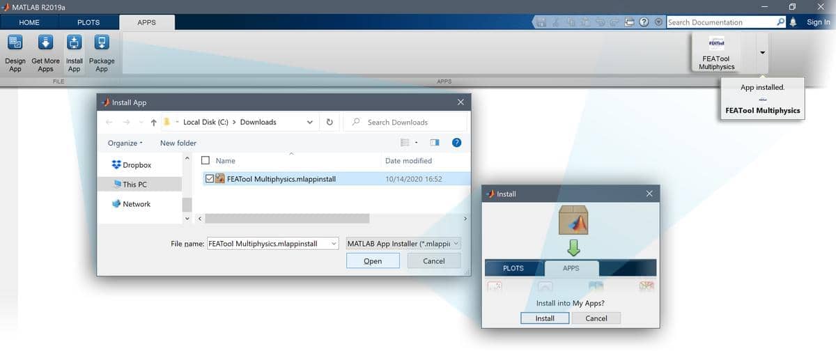
109 |
110 | Once the toolbox has been installed, an app icon will be available in
111 | the _APPS_ toolbar to start the _CFDTool_ GUI. (Note that MATLAB® may
112 | not show or give any indication of the toolbox installation progress
113 | or completion.)
114 |
115 |
116 | [OpenFOAM® CFD Solver](https://featool.com/doc/openfoam.html)
117 | --------------------
118 |
119 | The optional OpenFOAM CFD solver integration makes it easy to perform
120 | both laminar and turbulent high performance CFD simulations. OpenFOAM
121 | CFD simulations often results in a magnitude or more speedup for
122 | instationary simulations compared to the built-in flow
123 | solvers. Additionally, with the multi-simulation solver integration in
124 | _CFDTool_ it is possible to compare and better validate simulation
125 | results obtained using both the built-in and OpenFOAM CFD solvers.
126 |
127 | The OpenFOAM solver binaries are currently not included with _CFDTool_
128 | and must be installed separately. The OpenFOAM solver integration has
129 | been verified with OpenFOAM versions 2021 and 9. For Microsoft Windows
130 | systems it is recommended to install and use the pre-compiled
131 | Native-windows/mingw binaries available from
132 | [OpenCFD ESI](https://develop.openfoam.com/Development/openfoam/-/wikis/precompiled/windows),
133 | or the distribution from the
134 | [OpenFOAM Foundation](https://openfoam.org/download)
135 | for Linux and MacOS systems.
136 |
137 |
138 | Basic Use
139 | ---------
140 |
141 | _CFDTool_ and its GUI has been specifically designed to be as easy to
142 | use as possible, and making learning CFD simulation by experimentation
143 | easy.
144 |
145 | The modeling process is divided into six different steps or modes
146 |
147 | - **Geometry** - Definition of the geometry to be modeled
148 | - **Grid** - Subdivision of the geometry into smaller cells suitable
149 | for computation
150 | - **Equation** - Specification of material parameters and coefficients
151 | - **Boundary** - Boundary conditions specify how the model interacts
152 | with the surrounding environment (outside the geometry)
153 | - **Solve** - Solution and simulation of the defined model problem
154 | - **Post** - Visualization and postprocessing
155 |
156 | These modes can be accessed by clicking on the corresponding buttons
157 | in left hand side _Mode_ toolbar. The different modes may have
158 | specialized and different _Tools_ available in the corresponding
159 | toolbar. Advanced mode options may also be available in the
160 | corresponding menus.
161 |
162 | A number of pre-defined fluid flow and heat transfer tutorial examples
163 | are available under the **File** > **Model Examples and Tutorials...**
164 | menu option.
165 |
166 | Basic use and how to set up and model turbulent flow past a
167 | backwards facing step with OpenFOAM is explained in the
168 | [linked video tutorial](https://youtu.be/gHGttc31xj0)
169 | (click on the image below to start the tutorial).
170 |
171 |
172 |
173 | 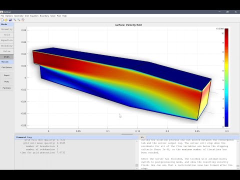 175 |
176 |
175 |
176 |
177 |
178 |
179 | Documentation
180 | -------------
181 |
182 | The _FEATool_
183 | [documentation](https://www.featool.com/doc),
184 | which shares most functionality with _CFDTool_, is available online,
185 | and also by selecting the corresponding option in the _Help_ menu of
186 | the _CFDTool_ GUI.
187 |
188 |
189 | License
190 | -------
191 |
192 | (C) Copyright 2013-2025 by Precise Simulation Limited.
193 | All Rights Reserved.
194 |
195 | CFDTool™ and FEATool Multiphysics™ are trademarks of Precise
196 | Simulation Limited. MATLAB® is a registered trademark of The
197 | MathWorks, Inc. OPENFOAM® is a registered trade mark of OpenCFD
198 | Limited. All other trademarks are the property of their respective
199 | owners. Precise Simulation Ltd and its products are not affiliated
200 | with, endorsed by, sponsored by these trademark owners.
201 |
202 | The license agreement for using CFDTool™ is included with the
203 | distribution and can also be accessed from the _Help_ menu in the
204 | application.
205 |
206 | Carefully read the license terms and conditions before installing or
207 | using the programs or documentation. Installing or using the programs
208 | means you have accepted and agree to be bound by the terms and
209 | conditions of this agreement. if you do not accept them, uninstall,
210 | remove and completely delete the programs and documentation.
211 |
--------------------------------------------------------------------------------
/THIRDPARTY:
--------------------------------------------------------------------------------
https://raw.githubusercontent.com/precise-simulation/cfdtool/fcb49b56030975c3609fedf0c7455b5f461104c0/THIRDPARTY
--------------------------------------------------------------------------------
/cfdtool.m:
--------------------------------------------------------------------------------
1 | %Start CFDTool.
2 | %
3 | % This command starts the main application GUI. The toolbox can
4 | %
5 | %
6 | % cfdtool test % Run all test suites
7 | % cfdtool testt % Run tests for GUI tutorials
8 | %
9 | %
10 | % and optionally with a vector specifying which tests to run
11 | %
12 | % cfdtool test/testt [#] % Run selected tests for test suite
13 | %
14 | % To automatically load a model file or (.fes) script on startup use
15 | %
16 | % cfdtool filename % Start GUI and load model
17 | %
18 | % Furthermore, the following maintenance tasks can also be performed
19 | %
20 | % cfdtool activate % Activate product license
21 | % cfdtool deactivate % Release/free activated license
22 | % cfdtool sysinfo % Print system information
23 |
24 | % Copyright 2013-2025 Precise Simulation, Ltd.
--------------------------------------------------------------------------------
/download.png:
--------------------------------------------------------------------------------
https://raw.githubusercontent.com/precise-simulation/cfdtool/fcb49b56030975c3609fedf0c7455b5f461104c0/download.png
--------------------------------------------------------------------------------
/screenshot.jpg:
--------------------------------------------------------------------------------
https://raw.githubusercontent.com/precise-simulation/cfdtool/fcb49b56030975c3609fedf0c7455b5f461104c0/screenshot.jpg
--------------------------------------------------------------------------------
/tutorials/01_Quickstart/02_heat_exchanger1.fes:
--------------------------------------------------------------------------------
1 | {"meta":{"app":"CFDTool","author":"Precise Simulation","build":"1.9.1","date":"17-Jan-2019","descr":["This heat exchanger example illustrates multiphysics modeling capabilities of CFDTool. The model consists of a series of heated pipes surrounded by a fluid at a lower temperature, and features effects of both free and forced convection. Two types of physical phenomena are considered, fluid flow which is modeled by the Navier-Stokes equations, and heat transfer modeled by a convection and conduction transport equation for the temperature. This system features a two-way multiphysics coupling, the fluid is coupled to and transports the temperature field, and the temperature is also coupled back to the fluid via the Boussinesq approximation accounting for buoyancy effects.","","Due to symmetry one can simplify the full geometry and only study a two dimensional slice between the heated pipes. The geometry will therefore consist of a _0.0075_ by _0.05 m_ rectangle from which a half circle with radius _0.003 m_ centered at _(0, 0.02)_ is removed. The mechanism for heating the pipes is not taken in consideration and are thus assumed to be at a fixed temperature of _Th = 330 K_. A cooling fluid flows from the bottom to the top and has an inlet temperature of _Tc = 300 K_. The other fluid and material parameters can be found in the model tutorial."],"dim":2,"image":"heat_exchanger1.jpg","keyw":["quickstart","heat_exchanger"],"mlver":"R2019a","name":"heat_exchanger1","phys":["Heat Transfer","Navier-Stokes Equations"],"system":"","time":737442,"title":"Heat Exchanger","type":"Multiphysics","user":"precsim","ver":[1,9,1]},
2 | "fields":["type","id","ui_arg","fcn_type","fcn_oarg"],
3 | "data":[
4 | ["introdlg","02_heat_exchanger1.fes",""],
5 | ["overlay",["Quickstart Tutorial","Natural and Forced Convection in a Heat Exchanger"],""],
6 | ["overlay",["","This heat exchanger model consists of a low temperature coolant flowing around a series of heated pipes. The multiphysics simulation involves both natural convection, through buoyancy effects, as well as forced convection, by coupling transport of the temperature field with the fluid flow."],""],
7 | ["msgbox","This tutorial can be run by selecting , **Model Examples and Tutorials...** >, **Quickstart** >, **Heat Exchanger** , from the **File** menu, and followed with the step-by-step instructions in the _User'susers Guide_.",""],
8 | ["pause","","2"],
9 | ["introdlg","close",""],
10 | ["uipushtool","Standard.NewFigure",[],"ClickedCallback",[]],
11 | ["uicontrol","radio_2d",0,"Callback",[]],
12 | ["uitext",[],"Select the **Navier-Stokes Equations** physics mode from the _Select Physics_ drop-down menu. An additional physics mode will be added later to couple and model heat transfer effects."],
13 | ["uicontrol*","popup_physsel",["Navier-Stokes Equations"],"Callback",[]],
14 | ["imgcap"],
15 | ["uicontrol","button_dlgnew_ok",[],"Callback",[]],
16 | ["overlay",["Geometry Mode",""],1],
17 | ["uitext*",[],"Only the fluid surrounding the heat exchanger will be modeled. And by using all symmetry planes, the geometry can be simplified to a two-dimensional planar cross section, which can be constructed by making a rectangle from which a circle is subtracted."],
18 | ["uicontrol","button_rectangle",[],"Callback",[0,1,0,1,"R1"]],
19 | ["uitext",[],"The geometry object properties must now be edited to set the correct size and position of the rectangle. To do this, click on the rectangle **R1** to select it, which also highlights it in red. Then click on the **Inspect/edit selected geometry object** _Toolbar_ button, and change the _min_ and _max_ coordinates of the rectangle, so they span between `0` and `0.0075` in the x-direction, and `0` and `0.05` in the y-direction."],
20 | ["uicontrol*","list_select_gobj",["R1"],"Callback",[]],
21 | ["imgcap"],
22 | ["uicontrol*","button_edit_gobj",[],"Callback",[]],
23 | ["uicontrol*","edit_x_min","0","Callback",[]],
24 | ["uicontrol*","edit_x_max","0.0075","Callback",[]],
25 | ["uicontrol*","edit_y_min","0","Callback",[]],
26 | ["uicontrol*","edit_y_max","0.05","Callback",[]],
27 | ["imgcap"],
28 | ["uicontrol*","button_dlggobj_ok",[],"Callback",[]],
29 | ["uitext",[],"Create a circle with center at _(0, 0.02)_, and radius equal to _0.003_."],
30 | ["uimenu",["Geometry","Create Object...","Circle"],[],"Callback",[]],
31 | ["uicontrol","edit_center","0 0.02","Callback",[]],
32 | ["uicontrol","edit_radius","0.003","Callback",[]],
33 | ["imgcap"],
34 | ["uicontrol","button_dlggobj_ok",{},"Callback",{}],
35 | ["uitext",[],"To subtract the circle from the rectangle, first select both geometry objects by clicking on them, so that both are highlighted in red, and then click on the **- / Subtract geometry objects** button. (Alternatively, if the circle is obscured by the rectangle, they can be selected by holding the _Ctrl_ key, while clicking on the labels **R1** and **C1** in the Selection list box, or in this case simply pressing _Ctrl + A_ to select all objects)."],
36 | ["uicontrol*","list_select_gobj",["R1","C1"],"Callback",[]],
37 | ["uicontrol*","button_subtract_gobj",[],"Callback",[]],
38 | ["imgcap"],
39 | ["uicontrol","button_grid_mode",1,"Callback",[]],
40 | ["uitext*",[],"The default grid may be too coarse to ensure an accurate solution. Decreasing the grid size and generating a finer grid can resolve curved boundaries better."],
41 | ["uicontrol","grid_hmax","0.0005"],
42 | ["uitext",[],"Press the **Generate** button to call the automatic grid generation algorithm."],
43 | ["uicontrol*","grid_generate",[],"Callback",[]],
44 | ["imgcap"],
45 | ["uicontrol","button_equation_mode",1,"Callback",[]],
46 | ["uitext",[],"Equation and material coefficients are specified in _Equation/Subdomain_ mode. In the Equation Settings dialog box, enter the following coefficients, `rho` for the density, `mu` for the viscosity, and `alpha*g*rho*(T-Tc)`alpha g rho T minus Tc for the volume and buoyancy force in the y-direction."],
47 | ["uicontrol*","rho_ns","rho","Callback",[]],
48 | ["uicontrol*","miu_ns","mu","Callback",[]],
49 | ["uicontrol*","Fy_ns","alpha*g*rho*(T-Tc)","Callback",[]],
50 | ["imgcap"],
51 | ["uitext",[],"An equation and physics mode for simulation of heat transfer effects must also be added. To access the multiphysics selection and add another physics mode, press the plus **+** tab and select **Heat Transfer** from the _Select Physics_ drop-down menu. Add the selection by pressing the **Add Physics >>>** button."],
52 | ["uicontrol*","tab_+",0,"Callback",[]],
53 | ["uicontrol*","popup_physsel",["Heat Transfer"],"Callback",[]],
54 | ["imgcap"],
55 | ["uicontrol*","button_addphys",[],"Callback",[]],
56 | ["uitext*",[],"Note that each physics mode will have its own tab for _Subdomain and Equation_ settings, as well as _Boundary_ conditions. Moreover, CFDTool works with any unit system, and it is up to the user to use consistent units for geometry dimensions, material, equation, and boundary coefficients."],
57 | ["uitext",[],"In the _Equation Settings_ tab for the heat transfer physics mode (labeled **ht**), set the _density_ to `rho`, _heat capacity_ to `cp`, and _thermal conductivity_ to `k`, respectively. The convective velocities should be coupled from the Navier-Stokes equations physics mode, to do this enter `u` and `v` in the corresponding edit fields (,as these are the default names of the dependent variables for the velocities). Press **OK** to finish with the equation coefficient specifications."],
58 | ["uicontrol*","rho_ht","rho","Callback",[]],
59 | ["uicontrol*","cp_ht","cp","Callback",[]],
60 | ["uicontrol*","k_ht","k","Callback",[]],
61 | ["uicontrol*","u_ht","u","Callback",[]],
62 | ["uicontrol*","v_ht","v","Callback",[]],
63 | ["imgcap"],
64 | ["uicontrol*","button_dlgeqn_ok",[],"Callback",[]],
65 | ["uitext*",[],"The _Model Constants and Expressions_ functionality can be used to define and store convenient expressions which then are available in the point, equation, boundary coefficients, and as postprocessing expressions. Here it is used to define the material and fluid parameters."],
66 | ["uitext",[],["Press the **Constants** _Toolbar_ button, or select the corresponding entry from the _Equation_ menu, and enter the following variables in the _Model Constants and Expressions_ dialog box. Press _Enter_ after the last expression or use the **Add Row** button to expand the expression list.","| Name | Expression |","|---------|------------|","| rho | 22 |","| mu | 2.8e-3 |","| alpha | 0.26e-3 |","| g | 9.81 |","| Tc | 300 |","| vin | 40e-2 |","| k | 0.55 |","| cp | 3.1e3 |","| Th | 330 |"]],
67 | ["uicontrol*","button_const_expr",[],"Callback",[]],
68 | ["uicontrol*","edit_dlgexpr_11","rho","Callback",[]],
69 | ["uicontrol*","edit_dlgexpr_12","22","Callback",[]],
70 | ["uicontrol*","edit_dlgexpr_21","mu","Callback",[]],
71 | ["uicontrol*","edit_dlgexpr_22","2.8e-3","Callback",[]],
72 | ["uicontrol*","edit_dlgexpr_31","alpha","Callback",[]],
73 | ["uicontrol*","edit_dlgexpr_32","0.26e-3","Callback",[]],
74 | ["uicontrol*","edit_dlgexpr_41","g","Callback",[]],
75 | ["uicontrol*","edit_dlgexpr_42","9.81","Callback",[]],
76 | ["uicontrol*","edit_dlgexpr_51","Tc","Callback",[]],
77 | ["uicontrol*","edit_dlgexpr_52","300","Callback",[]],
78 | ["uicontrol*","edit_dlgexpr_61","vin","Callback",[]],
79 | ["uicontrol*","edit_dlgexpr_62","40e-2","Callback",[]],
80 | ["uicontrol*","edit_dlgexpr_71","k","Callback",[]],
81 | ["uicontrol*","edit_dlgexpr_72","0.55","Callback",[]],
82 | ["uicontrol*","edit_dlgexpr_81","cp","Callback",[]],
83 | ["uicontrol*","edit_dlgexpr_82","3.1e3","Callback",[]],
84 | ["uicontrol*","edit_dlgexpr_91","Th","Callback",[]],
85 | ["uicontrol*","edit_dlgexpr_92","330","Callback",[]],
86 | ["imgcap"],
87 | ["uicontrol*","button_dlgexpr_ok",[],"Callback",[]],
88 | ["uicontrol","button_boundary_mode",1,"Callback",[]],
89 | ["uitext*",[],"Boundary conditions are defined in _Boundary Mode_ and describes how the model interacts with the external environment."],
90 | ["uitext",[],"First select the tab labeled **ns**, which allows for specifying boundary conditions for the Navier-Stokes equations physics mode. Then select all vertical boundaries (here **2**, **4**, and **7**, highlighting them in red), and choose **Symmetry/slip** from the drop down box. Switch to the heat transfer physics mode by selecting the **ht** tab, and choose the **Thermal insulation/symmetry** boundary condition."],
91 | ["uicontrol*","list_seldom",["2","4","7"],"Callback",[]],
92 | ["uicontrol*","popup_selbc_ns",["Symmetry/slip"],"Callback",[]],
93 | ["imgcap"],
94 | ["uicontrol*","tab_ht",0,"Callback",[]],
95 | ["uicontrol*","popup_selbc_ht",["Thermal insulation/symmetry"],"Callback",[]],
96 | ["uitext",[],"Continue with the top boundary (number **3**) which is the outflow. Select **Outflow/pressure** for the Navier-Stokes physics mode, and **Convective flux/outflow** for the heat transfer mode."],
97 | ["uicontrol*","list_seldom",["3"],"Callback",[]],
98 | ["uicontrol*","tab_ns",0,"Callback",[]],
99 | ["uicontrol*","popup_selbc_ns",["Outflow/pressure"],"Callback",[]],
100 | ["uitext",[],"The bottom boundary (number **1**) is the inflow and should be prescribed with the constant velocity `vin`v in in the y-direction, by using the **Inlet/velocity** condition. The **Temperature** should here be fixed to the cold/low temperature, `Tc`."],
101 | ["uicontrol*","list_seldom",["1"],"Callback",[]],
102 | ["uicontrol*","popup_selbc_ns",["Inlet/velocity"],"Callback",[]],
103 | ["uicontrol*","edit_bccoef2_ns","vin","Callback",[]],
104 | ["uicontrol*","tab_ht",0,"Callback",[]],
105 | ["uicontrol*","popup_selbc_ht",["Temperature"],"Callback",[]],
106 | ["uicontrol*","edit_bccoef1_ht","Tc","Callback",[]],
107 | ["uitext",[],"Lastly, the boundaries on the cylinder (**5** and **6**) are walls, and should be prescribed with **Wall/no-slip** boundary conditions for the velocity. For the **Temperature** the constant high temperature, `Th`, should be prescribed."],
108 | ["uicontrol*","list_seldom",["5","6"],"Callback",[]],
109 | ["uicontrol*","popup_selbc_ht",["Temperature"],"Callback",[]],
110 | ["uicontrol*","edit_bccoef1_ht","Th","Callback",[]],
111 | ["uicontrol*","tab_ns",0,"Callback",[]],
112 | ["uicontrol*","popup_selbc_ns",["Wall/no-slip"],"Callback",[]],
113 | ["imgcap"],
114 | ["uicontrol*","button_dlgbdr_ok",[],"Callback",[]],
115 | ["overlay",["Solve Mode",""],1],
116 | ["uitext",[],"Now that the problem is fully specified, press the **Solve** _Mode Toolbar_ button to switch to solve mode. Then press the **=** _Tool_ button , with an equals too sign, to call the solver with the default solver settings."],
117 | ["uicontrol*","button_solve_mode",1,"Callback",[]],
118 | ["uicontrol*","button_solve",[],"Callback",[]],
119 | ["overlay",["Postprocessing Mode",""],1],
120 | ["uitext*",[],"From the visualization of the resulting flow field one can see that the flow is accelerated when it passes between the cylinders. To show the temperature field, open the **Plot Options** and postprocessing settings dialog box, and select to plot and visualize the **Temperature, T** as both _surface_ and _contour_ plots."],
121 | ["imgcap"],
122 | ["uicontrol*","button_post_settings",[],"Callback",[]],
123 | ["uicontrol*","post_surf",["Temperature, T"],"Callback",[]],
124 | ["uicontrol*","ffiso",1,"Callback",[]],
125 | ["uicontrol*","post_iso",["Temperature, T"],"Callback",[]],
126 | ["imgcap"],
127 | ["uicontrol*","button_dlgpost_ok",[],"Callback",[]],
128 | ["uitext*",[],"The temperature plot show that the fluid is heated around the hot cylinder and follows the flow upwards."],
129 | ["uitext*",[],"CFDTool also allows for advanced postprocessing such as boundary integration. Integrate the expression _(T-Tc)/w_, T minus T c divided by the width, over the outflow boundary (where _w = 0.0075_ is the width of the domain) to find the change in the mean temperature."],
130 | ["uimenu","Boundary Integration...",[],"Callback",[]],
131 | ["uicontrol","list_seldom",["3"],"Callback",[]],
132 | ["uicontrol","edit_intexpr","(T-Tc)/0.0075","Callback",[]],
133 | ["imgcap"],
134 | ["uitext",[],"Press **OK** or _Apply_ to calculate and show the result of the boundary integration."],
135 | ["uicontrol*","button_dlginteval_ok",[],"Callback",[]],
136 | ["uitext*",[],"From the result one can see that the mean temperature along the outflow boundary has risen by about _1.7_ degrees."],
137 | ["imgcap"],
138 | ["overlay",["","The tutorial is now complete, and the model can be saved as a binary file (_.fea_), exported as a MATLAB _m_-script file, or a GUI playback file (_.fes_)."],""],
139 | ["uivalidate*",[],"pass=0;try,pass=abs(intbdr('T-Tc',fea,3)/0.0075-1.7)/1.7<0.1;catch,end"]
140 | ]}
141 |
--------------------------------------------------------------------------------
/tutorials/01_Quickstart/03_axisymmetric_flow1.fes:
--------------------------------------------------------------------------------
1 | {"meta":{"app":"CFDTool","author":"Precise Simulation","build":"1.4","date":"02-Sep-2019","descr":["This example models fluid flow in a narrowing pipe section. The constriction of the pipe will accelerate the flow according to the venturi effect. As the fluid is assumed to be both incompressible and isothermal the problem is governed by the Navier-Stokes equations.","","An appropriate boundary condition for the symmetry boundary must be chosen. A homogeneous Neumann insulation/symmetry condition is typically employed for scalar equations, but in the case of fluid flow a slip condition preventing any radial velocity while allowing flow in the axial direction is appropriate.","","The geometry of the problem considers a 2:1 constriction with an initial pipe diameter of _d = 2 m_. The inlet velocity is assumed to be uniform _vin = v(z=0) = 1 m/s_ and the fluid has a density of _rho = 1 kg/m^3_ and viscosity _mu = 0.05 kg/ms_. This gives a Reynolds number of _Re = rho*v*d/mu = 40_, which should result in laminar flow with a parabolic outflow profile."],"dim":2.5,"image":"axisymmetric_flow1.jpg","keyw":["quickstart","axisymmetry","fluid_flow","customization","equation_editing","validation"],"mlver":"R2019a","name":"axisymmetric_flow1","phys":["Navier-Stokes Equations"],"system":"","time":737443,"title":"Axisymmetric Fluid Flow","type":"Fluid Dynamics","user":"precsim","ver":[1,4,0]},
2 | "fields":["type","id","ui_arg","fcn_type","fcn_oarg"],
3 | "data":[
4 | ["introdlg","03_axisymmetric_flow1.fes",""],
5 | ["overlay",["Quickstart Tutorial","Axisymmetric Fluid Flow"],""],
6 | ["overlay",["","This example models fluid flow in a narrowing circular pipe section. The constriction of the pipe will accelerate the flow due to the venturi effect. The model also shows how the PDE equations can easily be customized and modified, in this case to accommodate for the transformation to an axisymmetric coordinate system."],""],
7 | ["msgbox","This tutorial can be run by selecting , **Model Examples and Tutorials...** >, **Quickstart** >, **Axisymmetric Fluid Flow** , from the **File** menu, and followed with the step-by-step instructions in the _User'susers Guide_.",""],
8 | ["pause","","2"],
9 | ["introdlg","close",""],
10 | ["uipushtool","Standard.NewFigure",[],"ClickedCallback",[]],
11 | ["uitext",[],"Click on the **Axisymmetry** _Space Dimension_ selection button in the _New Model_ dialog box, and select **Navier-Stokes Equations** from the _Select Physics_ drop-down list. Leave the space dimension and dependent variable names to their default values. Finish the physics selection and close the dialog box by clicking on the **OK** button."],
12 | ["uicontrol","radio_axi",1,"Callback",[]],
13 | ["uicontrol*","popup_physsel",["Navier-Stokes Equations"],"Callback",[]],
14 | ["imgcap"],
15 | ["uicontrol*","button_dlgnew_ok",[],"Callback",[]],
16 | ["overlay",["Geometry Mode",""],1],
17 | ["uitext*",[],"The geometry of the pipe cross section can be created by making _1 x 2_ and _0.5 x 1_two rectangles aligned with the (_r = 0_) symmetry axis, and also a circle with radius _0.5_ centered at (_1, 2_), and finally subtracting the circle from the joined rectangles."],
18 | ["uicontrol","button_rectangle",[],"Callback",[0,1,0,1,"R1"]],
19 | ["uitext",[],"The geometry object properties must now be edited to set the correct size and position of the rectangle. To do this, click on the rectangle **R1** to select it, which also highlights it in red. Then click on the **Inspect/edit selected geometry object** _Toolbar_ button, and change the _min_ and _max_ coordinates of the rectangle so they span between `0` and `1` in the x-direction, and `0` and `2` in the y-direction."],
20 | ["uicontrol*","list_select_gobj",["R1"],"Callback",[]],
21 | ["uicontrol*","button_edit_gobj",[],"Callback",[]],
22 | ["uicontrol*","edit_x_min","0","Callback",[]],
23 | ["uicontrol*","edit_x_max","1","Callback",[]],
24 | ["uicontrol*","edit_y_min","0","Callback",[]],
25 | ["uicontrol*","edit_y_max","2","Callback",[]],
26 | ["imgcap"],
27 | ["uicontrol*","button_dlggobj_ok",[],"Callback",[]],
28 | ["uicontrol*","button_rectangle",[],"Callback",[-0.5,0.5,0.5,1.5,"R2"]],
29 | ["uitext",[],"Similarly, change the _x_min_ and _x_max_ properties of the second rectangle **R2** to `0` and `0.5`, and _y_min_ and _y_max_ to `2` and `3`."],
30 | ["uicontrol*","list_select_gobj",["R2"],"Callback",[]],
31 | ["uicontrol*","button_edit_gobj",[],"Callback",[]],
32 | ["uicontrol*","edit_x_min","0","Callback",[]],
33 | ["uicontrol*","edit_x_max","0.5","Callback",[]],
34 | ["uicontrol*","edit_y_min","2","Callback",[]],
35 | ["uicontrol*","edit_y_max","3","Callback",[]],
36 | ["imgcap"],
37 | ["uicontrol*","button_dlggobj_ok",[],"Callback",[]],
38 | ["uimenu*",["Geometry","Create Object...","Circle"],{},"Callback",{}],
39 | ["uicontrol*","edit_center","1 2","Callback",[]],
40 | ["uicontrol*","edit_radius","0.5","Callback",{}],
41 | ["imgcap"],
42 | ["uicontrol*","button_dlggobj_ok",[],"Callback",[]],
43 | ["imgcap"],
44 | ["uitext",[],"To create the combined geometry, select **Combine Objects...** from the _Geometry_ menu. Enter the formula `R1 + R2 - C1`R1 plus R2 minus C1 in the edit field of the _Combine Geometry Objects_ dialog box and press **OK**."],
45 | ["uimenu*","Combine Objects...",[],"Callback",[]],
46 | ["uicontrol*","edit_dlgedit","R1 + R2 - C1","Callback",[]],
47 | ["imgcap"],
48 | ["uicontrol*","button_dlgedit_ok",[],"Callback",[]],
49 | ["imgcap"],
50 | ["uicontrol","button_grid_mode",1,"Callback",[]],
51 | ["uitext*",[],"The default grid may be too coarse to ensure an accurate solution. Decreasing the grid size and generating a finer grid can resolve curved boundaries better."],
52 | ["uicontrol","grid_hmax","0.1"],
53 | ["uitext",[],"Press the **Generate** button to call the automatic grid generation algorithm."],
54 | ["uicontrol*","grid_generate",[],"Callback",[]],
55 | ["imgcap"],
56 | ["uicontrol","button_equation_mode",1,"Callback",[]],
57 | ["uitext",[],"Equation and material coefficients are specified in _Equation/Subdomain_ mode. In the Equation Settings dialog box enter `1` for the density and `5e-2` for the viscosity."],
58 | ["uitext*",[],"Note that CFDTool can work with any unit system, 4 it 02 Sep to the user to use consistent units for geometry dimensions, material, equation, and boundary coefficients."],
59 | ["uicontrol*","rho_ns","1","Callback",[]],
60 | ["uicontrol*","miu_ns","5e-2","Callback",[]],
61 | ["uitext",[],"Also select the **(P2P1/Q2Q1) second order conforming Stokes element** finite element discretization for higher accuracy, and to avoid having to reformulate the stabilization terms."],
62 | ["uicontrol*","popup_sfun_ns",["(P2P1/Q2Q1) second order conforming Stokes element"],"Callback",[]],
63 | ["imgcap"],
64 | ["uitext",[],"Press **OK** to finish with the equation editing and coefficient specifications."],
65 | ["uicontrol*","button_dlgeqn_ok",[],"Callback",[]],
66 | ["uitext",[],"Switch to boundary condition specification mode by clicking on **Boundary** the _Mode Toolbar_ button. In the _Boundary Settings_ dialog box, first choose all boundaries in the left hand side _Boundaries_ list box and select the **Wall/no-slip** boundary condition from the drop-down menu. Now select the lower inflow boundary (number **1**) in the left hand side Boundaries list box and select the **Inlet/velocity** boundary condition. Enter `1` in the edit field for the velocity _v0_ in the z-direction."],
67 | ["overlay",["Boundary Mode",""],1],
68 | ["uitext*",[],"Boundary conditions are defined in _Boundary Mode_ and describes how the model interacts with the external environment."],
69 | ["uitext",[],"Switch to boundary condition specification mode by clicking on **Boundary** the _Mode Toolbar_ button. In the _Boundary Settings_ dialog box, first choose all boundaries in the left hand side _Boundaries_ list box, and select the **Wall/no-slip** boundary condition from the drop-down menu. Then select the **Inlet/velocity** boundary condition for the lower inflow boundary (number **1**), and enter `1` in the edit field for the velocity _v0_v 0 in the z-direction."],
70 | ["uicontrol*","button_boundary_mode",1,"Callback",[]],
71 | ["uitext*",[],"Boundary conditions are defined in _Boundary Mode_ and describes how the model interacts with the external environment."],
72 | ["uicontrol*","list_seldom",["1"],"Callback",[]],
73 | ["uicontrol*","popup_selbc_ns",["Inlet/velocity"],"Callback",[]],
74 | ["uicontrol*","edit_bccoef2_ns","1","Callback",[]],
75 | ["imgcap"],
76 | ["uitext",[],"Select the top outflow boundary (number **5**) and the **Neutral outflow/stress boundary** condition from the drop-down menu (alternatively, it is also possible prescribe a pressure at the outflow with the _Outflow/pressure_ condition)."],
77 | ["uicontrol*","list_seldom",["5"],"Callback",[]],
78 | ["uicontrol*","popup_selbc_ns",["Neutral outflow/stress boundary"],"Callback",[]],
79 | ["uitext",[],"Lastly, select the left side boundaries on the symmetry axis (number **3** and **6**) and select the **Symmetry/slip** boundary condition from the drop-down menu. This will prevent flow in the radial direction while allowing it in the axial direction. Finish the boundary condition specification by clicking the **OK** button."],
80 | ["uicontrol*","list_seldom",["6","7"],"Callback",[]],
81 | ["uicontrol*","popup_selbc_ns",["Symmetry/slip"],"Callback",[]],
82 | ["imgcap"],
83 | ["uicontrol*","button_dlgbdr_ok",[],"Callback",[]],
84 | ["overlay",["Solve Mode",""],1],
85 | ["uitext",[],"Now that the problem has been defined, press the **Solve** _Mode Toolbar_ button to switch to solve mode, and press the **Settings** button to open the _Solver Settings_ dialog box."],
86 | ["uicontrol*","button_solve_mode",1,"Callback",[]],
87 | ["uicontrol*","button_solver_settings",[],"Callback",[]],
88 | ["uitext",[],"In the _Non-Linear Solver Settings_ section of the Solver Settings dialog box, increase the _Maximum non-linear iterations_ to `100`, and set the _Non-linear relaxation parameter_ to `0.8` to relax the convergence of the solver."],
89 | ["uicontrol*","maxnit","100","Callback",[]],
90 | ["uicontrol*","nlrlx","0.8","Callback",[]],
91 | ["imgcap"],
92 | ["uitext",[],"To start the solver with the chosen settings press the **Solve** button, or press **OK** and then the **=** _Toolbar_ button with an equals too sign."],
93 | ["uicontrol*","button_dlgsolversettings_solve",[],"Callback",[]],
94 | ["imgcap"],
95 | ["overlay",["Postprocessing Mode",""],1],
96 | ["uitext*",[],"After the problem has been solved CFDTool will automatically switch to postprocessing mode and display the computed velocity field, which clearly shows how the flow is significantly accelerated by the pipe constriction."],
97 | ["uitext*",[],"Cross sections of expressions such as the velocity profile can be plotted by using the **Point/Line Evaluation...** feature from the _Post_ menu."],
98 | ["uimenu","Point/Line Evaluation...",[],"Callback",[]],
99 | ["uitext",[],"Enter the evaluation coordinates `0:0.05:0.5`0 to 0.5 in steps of 0.05 and `2.8` in the _r_ and _z-directions_, respectively. These expressions give vectors of coordinates points to evaluate."],
100 | ["uicontrol*","edit_rcoord","0:0.05:0.5","Callback",[]],
101 | ["uicontrol*","edit_zcoord","2.8","Callback",[]],
102 | ["imgcap"],
103 | ["uitext",[],"Press _Apply_ or **OK** to create a new figure with the cross section plot."],
104 | ["uicontrol*","buttons_dlgpntline_ok",[],"Callback",[]],
105 | ["uitext*",[],"From the cross section plot, one can see that the velocity profile close to the outlet, at _z = 2.8_, is starting to shift from parabolic to a more square profile indicating a higher flow rate. This also suggests that one might need to study a longer outflow section to allow for a fully developed parabolic laminar flow profile."],
106 | ["imgcap"],
107 | ["figure*","Line Evaluation",{},"closeRequestFcn",{}],
108 | ["overlay",["","The tutorial is now complete, and the model can be saved as a binary file (_.fea_), exported as a MATLAB _m_-script file, or a GUI playback file (_.fes_)."],""],
109 | ["uivalidate*",[],"pass=0;try,r=linspace(0,1/2,20);z=0.9*3*ones(1,20);U=evalexpr('sqrt(u^2+w^2)',[r;z],fea).';U_ref=8*(1-4*r.^2);pass=sqrt(sum((U-U_ref).^2)/sum(U_ref.^2))<0.15;catch,end"]
110 | ]}
111 |
--------------------------------------------------------------------------------
/tutorials/01_Quickstart/04_natural_convection1.fes:
--------------------------------------------------------------------------------
1 | {"meta":{"app":"CFDTool","author":"Precise Simulation","build":"1.9.1","date":"16-Mar-2019","descr":["This multiphysics model illustrates natural convection effects in a unit square domain using the Boussinesq approximation. The model involves a Navier-Stokes equations physics mode, representing the fluid flow with solid wall or no-slip boundary conditions everywhere. In addition a heat transfer physics mode is added to model the temperature field . The top and bottom boundaries are perfectly insulated while the left boundary is prescribed a unit temperature and the right zero.","","The physics modes are two way coupled through the vertical source term in the Navier-Stokes equations, _Pr*Ra*T_, and the velocities transporting the temperature coming directly from the fluid flow. First, the Prandtl and Rayleigh numbers are set to _Pr = 0.71_ and _Ra = 1e3_, respectively, after which the _Ra_ number will be increased to _1e4_. The references contain benchmark reference and comparison results for a number of quantities such as maximum velocities and the Nusselt number [9,10].","","References:","","[9] D. de Vahl Davis, Natural Convection of Air in a Square Cavity - A Benchmark Solution, Int. J. Numer. Meth. Fluids, vol. 3, pp. 249-264, 1983.","","[10] D. de Vahl Davis and I. P. Jones, Natural Convection of Air in a Square Cavity - A Comparison Exercise, Int. J. Numer. Meth. Fluids, vol. 3, pp. 227-248, 1983."],"dim":2,"image":"natural_convection1.jpg","keyw":["natural_convection","validation"],"mlver":"R2018b","name":"natural_convection1","phys":["Heat Transfer","Navier-Stokes Equations"],"system":"","time":737501,"title":"Natural Convection in a Square Cavity","type":"Multiphysics","user":"precsim","ver":[1,9,1]},
2 | "fields":["type","id","ui_arg","fcn_type","fcn_oarg"],
3 | "data":[
4 | ["uipushtool","Standard.NewFigure",{},"ClickedCallback",{}],
5 | ["uicontrol","popup_physsel",["Navier-Stokes Equations"],"Callback",{}],
6 | ["imgcap"],
7 | ["uicontrol","button_dlgnew_ok",{},"Callback",{}],
8 | ["uimenu",["Geometry","Create Object...","Rectangle"],{},"Callback",{}],
9 | ["uicontrol","button_dlggobj_ok",{},"Callback",{}],
10 | ["uicontrol","button_grid_mode",1,"Callback",{}],
11 | ["uicontrol","grid_hmax","0.03"],
12 | ["uicontrol","grid_generate",{},"Callback",{}],
13 | ["imgcap"],
14 | ["uicontrol","button_equation_mode",1,"Callback",{}],
15 | ["uitext*",[],"The non-dimensionalized form of the Boussinesq source term _Pr*Ra*T_ couples the temperature to the y-direction source term of the Navier-Stokes equations."],
16 | ["uicontrol","Fy_ns","Pr*Ra*T","Callback",{}],
17 | ["imgcap"],
18 | ["uicontrol","tab_+",0,"Callback",{}],
19 | ["uitext*",[],"Add the heat transfer physics mode and coupled the velocities _u_ and _v_ to the convective transport terms."],
20 | ["uicontrol","popup_physsel",["Heat Transfer"],"Callback",{}],
21 | ["imgcap"],
22 | ["uicontrol","button_addphys",{},"Callback",{}],
23 | ["uicontrol","u_ht","u","Callback",{}],
24 | ["uicontrol","v_ht","v","Callback",{}],
25 | ["imgcap"],
26 | ["uicontrol","button_dlgeqn_ok",{},"Callback",{}],
27 | ["uitext",[],["Press the **Constants** _Toolbar_ button, or select the corresponding entry from the _Equation_ menu, and enter the following values for the Prandtl and Rayleigh numbers in the _Model Constants and Expressions_ dialog box.","| Name | Expression |","|------|------------|","| Pr | 0.71 |","| Ra | 1e3 |"]],
28 | ["uicontrol*","button_const_expr",{},"Callback",{}],
29 | ["uicontrol*","edit_dlgexpr_11","Pr","Callback",{}],
30 | ["uicontrol*","edit_dlgexpr_12","0.71","Callback",{}],
31 | ["uicontrol*","edit_dlgexpr_21","Ra","Callback",{}],
32 | ["uicontrol*","edit_dlgexpr_22","1e3","Callback",{}],
33 | ["imgcap"],
34 | ["uicontrol*","button_dlgexpr_ok",{},"Callback",{}],
35 | ["uicontrol","button_boundary_mode",1,"Callback",{}],
36 | ["uitext*",[],"Switch to the **ns** tab, which corresponds to the boundary conditions for the Navier-Stokes equations physics mode. Then select the **Wall/no-slip** for all four boundaries."],
37 | ["uitext*",[],"Click on the **ht** tab to change to specifying boundary conditions for the heat transfer physics mode. Select **Thermal insulation/symmetry** conditions for the top and bottom boundaries."],
38 | ["uicontrol","tab_ht",0,"Callback",{}],
39 | ["uicontrol","list_seldom",["1","3"],"Callback",{}],
40 | ["uitext*",[],"Select a **Temperature** boundary conditions for the left and right boundaries, and set a fixed temperature equal to _1_ at the left side."],
41 | ["uicontrol","popup_selbc_ht",["Thermal insulation/symmetry"],"Callback",{}],
42 | ["imgcap"],
43 | ["uicontrol","list_seldom",["4"],"Callback",{}],
44 | ["uicontrol","popup_selbc_ht",["Temperature"],"Callback",{}],
45 | ["uicontrol","edit_bccoef1_ht","1","Callback",{}],
46 | ["imgcap"],
47 | ["uicontrol","list_seldom",["2"],"Callback",{}],
48 | ["uicontrol","popup_selbc_ht",["Temperature"],"Callback",{}],
49 | ["imgcap"],
50 | ["uicontrol","button_dlgbdr_ok",{},"Callback",{}],
51 | ["uicontrol","button_solve_mode",1,"Callback",{}],
52 | ["uicontrol","button_solve",{},"Callback",{}],
53 | ["uitext*",[],"One can see how the temperature difference is causing a vortex in the flow field, which in turn causes an offset in the temperature field."],
54 | ["imgcap"],
55 | ["uitext*",[],"Change the plot to visualize the temperature field as surface and contour plots, and the velocity field as an arrow plot."],
56 | ["uicontrol","button_post_settings",{},"Callback",{}],
57 | ["uicontrol","ffarrow",1,"Callback",{}],
58 | ["uicontrol","post_surf",["Temperature, T"],"Callback",{}],
59 | ["uicontrol","ffiso",1,"Callback",{}],
60 | ["uicontrol","post_iso",["Temperature, T"],"Callback",{}],
61 | ["imgcap"],
62 | ["uicontrol","button_dlgpost_ok",{},"Callback",{}],
63 | ["imgcap"],
64 | ["uitext*",[],"Use the boundary integration postprocessing tool to calculate the average Nusselt number for the vertical boundaries, and compare it to the reference value of _1.118_."],
65 | ["uimenu",["Post","Boundary Integration..."],{},"Callback",{}],
66 | ["uicontrol","list_seldom",["2","4"],"Callback",{}],
67 | ["uicontrol","edit_intexpr","abs(Tx)/2","Callback",{}],
68 | ["uicontrol","button_dlginteval_apply",{},"Callback",{}],
69 | ["imgcap"],
70 | ["uicontrol","button_dlginteval_ok",{},"Callback",{}],
71 | ["uivalidate",[],"pass=0;try,Nu_mean=abs(intbdr('Tx/2',fea,[2,4],2));pass=abs(Nu_mean-1.118)/1.118<0.06;catch,end"],
72 | ["uitext*",[],"The simulation will now be repeated but with an increased Rayleigh number _Ra = 1e4_. Instead of starting over from the beginning the existing solution will be used as a starting guess which helps with non-linear convergence."],
73 | ["uimenu",["Equation","Model Constants and Expressions..."],{},"Callback",{}],
74 | ["uicontrol","edit_dlgexpr_22","1e4","Callback",{}],
75 | ["imgcap"],
76 | ["uicontrol","button_dlgexpr_ok",{},"Callback",{}],
77 | ["uicontrol","button_solve_mode",1,"Callback",{}],
78 | ["uitext*",[],"To assist with convergence, as well as selecting the old solution as initial value, also increase the non-linear relaxation and the maximum number of non-linear iterations."],
79 | ["uicontrol","button_solver_settings",{},"Callback",{}],
80 | ["uicontrol","init1",1,"Callback",{}],
81 | ["uicontrol","maxnit","100","Callback",{}],
82 | ["uicontrol","nlrlx","0.8","Callback",{}],
83 | ["imgcap"],
84 | ["uicontrol","button_dlgsolversettings_solve",{},"Callback",{}],
85 | ["uitext*",[],"It is evident that the increase in Rayleigh number causes a significantly stronger rotation and stretching of the temperature field."],
86 | ["imgcap"],
87 | ["uitext*",[],"Use boundary integration tool again to calculate the mean Nusselt number for the vertical boundaries, and compare it to the corresponding reference value of _2.243_ for _Ra = 1e4_."],
88 | ["uimenu",["Post","Boundary Integration..."],{},"Callback",{}],
89 | ["uicontrol","list_seldom",["2","4"],"Callback",{}],
90 | ["uicontrol","edit_intexpr","abs(Tx)/2","Callback",{}],
91 | ["uicontrol","button_dlginteval_apply",{},"Callback",{}],
92 | ["imgcap"],
93 | ["uicontrol","button_dlginteval_ok",{},"Callback",{}],
94 | ["uivalidate",[],"pass=0;try,Nu_mean=abs(intbdr('Tx/2',fea,[2,4],2));pass=abs(Nu_mean-2.243)/2.243<0.13;catch,end"]
95 | ]}
96 |
--------------------------------------------------------------------------------
/tutorials/01_Quickstart/axisymmetric_flow1.jpg:
--------------------------------------------------------------------------------
https://raw.githubusercontent.com/precise-simulation/cfdtool/fcb49b56030975c3609fedf0c7455b5f461104c0/tutorials/01_Quickstart/axisymmetric_flow1.jpg
--------------------------------------------------------------------------------
/tutorials/01_Quickstart/heat_exchanger1.jpg:
--------------------------------------------------------------------------------
https://raw.githubusercontent.com/precise-simulation/cfdtool/fcb49b56030975c3609fedf0c7455b5f461104c0/tutorials/01_Quickstart/heat_exchanger1.jpg
--------------------------------------------------------------------------------
/tutorials/01_Quickstart/natural_convection1.jpg:
--------------------------------------------------------------------------------
https://raw.githubusercontent.com/precise-simulation/cfdtool/fcb49b56030975c3609fedf0c7455b5f461104c0/tutorials/01_Quickstart/natural_convection1.jpg
--------------------------------------------------------------------------------
/tutorials/02_Heat_Transfer/01_heat_transfer1.fes:
--------------------------------------------------------------------------------
1 | {"meta":{"app":"CFDTool","author":"Precise Simulation","build":"1.9.1","date":"12-Feb-2019","descr":["Transient heat diffusion problem where a unit length rod is kept at fixed temperature _T = 25_ at the right end and losing heat from a constant outward heat flux _q_n=1_ at the other end. The computed results are compared with the analytic solution",""," Tref = (24+x) + sum(n=1,inf) 8/(1-2*n)^2/pi^2*cos((n-1/2)*pi*x)*exp(-((n-1/2)^2*pi^2)*t)"],"dim":1,"image":"heat_transfer1.jpg","keyw":["heat_diffusion","validation"],"mlver":"R2019a","name":"heat_transfer1","phys":["Heat Transfer"],"system":"","time":737468,"title":"Transient Heat Diffusion in a Rod","type":"Heat Transfer","user":"precsim","ver":[1,9,1]},
2 | "fields":["type","id","ui_arg","fcn_type","fcn_oarg"],
3 | "data":[
4 | ["uipushtool","Standard.NewFigure",[],"ClickedCallback",[]],
5 | ["uicontrol","radio_1d",1,"Callback",[]],
6 | ["uicontrol","popup_physsel",["Heat Transfer"],"Callback",[]],
7 | ["imgcap"],
8 | ["uicontrol","button_dlgnew_ok",[],"Callback",[]],
9 | ["uicontrol","button_line",[],"Callback",[]],
10 | ["uicontrol","button_linegeom_ok",[],"Callback",[]],
11 | ["imgcap"],
12 | ["uicontrol","button_grid_mode",1,"Callback",[]],
13 | ["uicontrol","grid_generate",[],"Callback",[]],
14 | ["imgcap"],
15 | ["uicontrol","button_equation_mode",1,"Callback",[]],
16 | ["uicontrol","eqn_init1_ht","25","Callback",[]],
17 | ["imgcap"],
18 | ["uicontrol","button_dlgeqn_ok",[],"Callback",[]],
19 | ["uitext*",[],"A convenient way to define and store coefficients, variables, and expressions is using the _Model Constants and Expressions_ functionality. The defined expressions can then be used in point, equation, boundary coefficients, as well as postprocessing expressions, and can easily be changed and updated in a single place. Enter an the expression for the reference temperature _Tref_ with two terms _n = 2_."],
20 | ["uicontrol","button_const_expr",[],"Callback",[]],
21 | ["uicontrol","edit_dlgexpr_11","Tref","Callback",[]],
22 | ["uicontrol","edit_dlgexpr_12","(24+x) + 8/pi^2*cos(pi/2*x)*exp(-pi^2/4*t) + 8/9/pi^2*cos(3*pi/2*x)*exp(-(9/4*pi^2)*t) ","Callback",[]],
23 | ["imgcap"],
24 | ["uicontrol","button_dlgexpr_ok",[],"Callback",[]],
25 | ["uicontrol","button_boundary_mode",1,"Callback",[]],
26 | ["uicontrol","list_seldom",["1"],"Callback",[]],
27 | ["uicontrol","popup_selbc_ht",["Heat flux"],"Callback",[]],
28 | ["uicontrol","edit_bccoef1_ht","-1","Callback",[]],
29 | ["imgcap"],
30 | ["uicontrol","list_seldom",["2"],"Callback",[]],
31 | ["uicontrol","popup_selbc_ht",["Temperature"],"Callback",[]],
32 | ["uicontrol","edit_bccoef1_ht","25","Callback",[]],
33 | ["imgcap"],
34 | ["uicontrol","button_dlgbdr_ok",[],"Callback",[]],
35 | ["uicontrol","button_solve_mode",1,"Callback",[]],
36 | ["uicontrol","button_solver_settings",[],"Callback",[]],
37 | ["uicontrol","solver",[" Time-Dependent"],"Callback",[]],
38 | ["uicontrol","tstep","0.01","Callback",[]],
39 | ["uicontrol","tmax","0.2","Callback",[]],
40 | ["imgcap"],
41 | ["uicontrol","button_dlgsolversettings_solve",[],"Callback",[]],
42 | ["imgcap"],
43 | ["uicontrol","button_post_settings",[],"Callback",[]],
44 | ["uitext*",[],"The temperature at the final time is shown where one can see that the temperature is a constant 25 degrees at the right end and is losing heat towards the left."],
45 | ["uitext*",[],"Plot and visualize the difference between the computed and reference temperature fields."],
46 | ["uicontrol","ssurfexpr","T-Tref","Callback",[]],
47 | ["imgcap"],
48 | ["uicontrol","button_dlgpost_ok",[],"Callback",[]],
49 | ["uimenu",["Options","Axis/Grid Settings..."],[],"Callback",[]],
50 | ["uicontrol*","opt_dlgax_faxeq",1,"Callback",[]],
51 | ["uicontrol*","opt_dlgax_fbbox",0,"Callback",[]],
52 | ["uicontrol","opt_dlgax_faxis",1,"Callback",[]],
53 | ["uitext",[],"Enter `0 1 -1e-3 1e-3`zero, 1, minus 1 e minus 3, 1 e minus 3 into the edit field for the _Axis limits_ (for the _xmin_, _xmax_, _ymin_, and _ymax_ limits)."],
54 | ["uicontrol*","opt_dlgax_axis","0 1 -1e-3 1e-3","Callback",[]],
55 | ["imgcap"],
56 | ["uicontrol","button_dlgax_ok",[],"Callback",[]],
57 | ["uitext*",[],"The error already has a small magnitude of _1e-3_ but could be improved with a smaller grid size, higher element order, and smaller time step size."],
58 | ["imgcap"],
59 | ["uivalidate",[],"pass=0;try,pass=norm(evalexprp('abs(T-Tref)/abs(Tref)',fea))<1e-3;catch,end"]
60 | ]}
61 |
--------------------------------------------------------------------------------
/tutorials/02_Heat_Transfer/02_heat_transfer2.fes:
--------------------------------------------------------------------------------
1 | {"meta":{"app":"CFDTool","author":"Precise Simulation","build":"1.9.1","date":"12-Feb-2019","descr":["Two dimensional heat transfer of a ceramic strip with both radiation and convection on the top boundary. The ceramic has a thermal conductivity of _3 W/mK_ and the sides are fixed at a temperature of _900 C_ while the bottom boundary is insulated. The surrounding temperature is _50 C_. The top boundary is exposed to both natural convection (with a film coefficient _h = 50 W/m^2K_) and radiation (with emissivity epsilon = 0.7 and the Stefan-Boltzmann _5.669e-8 W/m^2K^4_). The solution is sought at three points along the vertical symmetry line.","","Reference:","","[1] Holman, J. P., Heat Transfer, Fifth Edition, New York: McGraw-Hill, 1981, page 96, Example 3-8."],"dim":2,"image":"heat_transfer2.jpg","keyw":["heat_diffusion","radiation","convection"],"mlver":"R2019a","name":"heat_transfer2","phys":["Heat Transfer"],"system":"","time":737468,"title":"Heat Transfer in a Ceramic Strip","type":"Heat Transfer","user":"precsim","ver":[1,9,1]},
2 | "fields":["type","id","ui_arg","fcn_type","fcn_oarg"],
3 | "data":[
4 | ["uipushtool","Standard.NewFigure",[],"ClickedCallback",[]],
5 | ["uicontrol","popup_physsel",["Heat Transfer"],"Callback",[]],
6 | ["uicontrol","button_dlgnew_ok",[],"Callback",[]],
7 | ["uicontrol","button_rectangle",[],"Callback",[0,1,0,1,"R1"]],
8 | ["uicontrol","list_select_gobj",["R1"],"Callback",[]],
9 | ["uicontrol","button_edit_gobj",[],"Callback",[]],
10 | ["uicontrol","edit_x_min","0","Callback",[]],
11 | ["uicontrol","edit_x_max","0.02","Callback",[]],
12 | ["uicontrol","edit_y_min","0","Callback",[]],
13 | ["uicontrol","edit_y_max","0.01","Callback",[]],
14 | ["uicontrol","button_dlggobj_ok",[],"Callback",[]],
15 | ["uicontrol","button_grid_mode",1,"Callback",[]],
16 | ["uicontrol","grid_hmax","0.001"],
17 | ["uicontrol","grid_generate",[],"Callback",[]],
18 | ["uicontrol","button_equation_mode",1,"Callback",[]],
19 | ["uicontrol","k_ht","3","Callback",[]],
20 | ["uicontrol","button_dlgeqn_ok",[],"Callback",[]],
21 | ["uicontrol","button_boundary_mode",1,"Callback",[]],
22 | ["uicontrol","list_seldom",["1"],"Callback",[]],
23 | ["uicontrol","popup_selbc_ht",["Thermal insulation/symmetry"],"Callback",[]],
24 | ["uicontrol","list_seldom",["2","4"],"Callback",[]],
25 | ["uicontrol","popup_selbc_ht",["Temperature"],"Callback",[]],
26 | ["uicontrol","edit_bccoef1_ht","900+273","Callback",[]],
27 | ["uicontrol","list_seldom",["3"],"Callback",[]],
28 | ["uicontrol","popup_selbc_ht",["Heat flux"],"Callback",[]],
29 | ["uicontrol","edit_bccoef2_ht","50","Callback",[]],
30 | ["uicontrol","edit_bccoef3_ht","50+273","Callback",[]],
31 | ["uicontrol","edit_bccoef4_ht","0.7*5.669e-8","Callback",[]],
32 | ["uicontrol","edit_bccoef5_ht","50+273","Callback",[]],
33 | ["uicontrol","button_dlgbdr_ok",[],"Callback",[]],
34 | ["uicontrol","button_solve_mode",1,"Callback",[]],
35 | ["uicontrol","button_solve",[],"Callback",[]],
36 | ["imgcap"],
37 | ["uitext*",[],"Evaluate the temperature in the points _(0.01, 0.01)_, _(0.01, 0.005)_, and _(0.01, 0)_ and compare with the reference values _Tref = 984_, _1064_, and _1088_."],
38 | ["uimenu",["Post","Point/Line Evaluation..."],[],"Callback",[]],
39 | ["uicontrol","edit_xcoord","0.01","Callback",[]],
40 | ["uicontrol","edit_ycoord","0.01","Callback",[]],
41 | ["uicontrol","buttons_dlgpntline_apply",[],"Callback",[]],
42 | ["uicontrol","edit_ycoord","0.005","Callback",[]],
43 | ["uicontrol","buttons_dlgpntline_apply",[],"Callback",[]],
44 | ["uicontrol","edit_ycoord","0","Callback",[]],
45 | ["uicontrol","buttons_dlgpntline_apply",[],"Callback",[]],
46 | ["uicontrol","buttons_dlgpntline_ok",[],"Callback",[]],
47 | ["uivalidate",[],"pass=0;try,T=evalexpr('T',[0.01,0.01,0.01;0.01,0.005,0],fea);Tref=[984,1064,1088]';err=norm(abs(T-Tref)./Tref);pass=err<0.01;catch,end"]
48 | ]}
49 |
--------------------------------------------------------------------------------
/tutorials/02_Heat_Transfer/03_heat_transfer3.fes:
--------------------------------------------------------------------------------
1 | {"meta":{"app":"CFDTool","author":"Precise Simulation","build":"1.9.1","date":"12-Feb-2019","descr":["This example models shrink fitting of a two part assembly. A chilled tungsten rod is inserted into a slot in a heated steel frame. The rod can be fitted due to thermal expansion of the frame, and when the assembly reaches equilibrium temperature the two parts will be joined due to the ensuing pressure fit.","","This model illustrates how to simulate the transient heat transfer process with two domains of different materials. The assembly is cooled due to convection through a surrounding medium, and the time when the maximum temperature has reached _70 C_ should be determined."],"dim":2,"image":"heat_transfer3.jpg","keyw":["shrink_fitting","assembly","cooling"],"mlver":"R2019a","name":"heat_transfer3","phys":["Heat Transfer"],"system":"","time":737468,"title":"Shrink Fitting of an Assembly","type":"Heat Transfer","user":"precsim","ver":[1,9,1]},
2 | "fields":["type","id","ui_arg","fcn_type","fcn_oarg"],
3 | "data":[
4 | ["introdlg","03_heat_transfer3.fes",""],
5 | ["overlay",["Heat Transfer Tutorial","Shrink Fitting of an Assembly"],""],
6 | ["overlay",["","This example models shrink fitting of a two part assembly. A chilled tungsten rod is inserted into a slot in a heated steel frame. The rod can be fitted due to thermal expansion of the frame, and when the assembly reaches equilibrium temperature, the two parts will be joined due to the ensuing pressure fit."],""],
7 | ["overlay",["","This model illustrates how to simulate the transient heat transfer process with two domains of different materials. The assembly is cooled due to convection through a surrounding medium, and the time when the maximum temperature has reached _ 70Cdegrees_ should be determined."],""],
8 | ["msgbox","This tutorial can be run by selecting , **Model Examples and Tutorials...** >, **Heat Transfer** >, **Shrink Fitting of an Assembly** , from the **File** menu, and followed along with the step-by-step instructions in the _User'susers Guide_.",""],
9 | ["pause","","2"],
10 | ["introdlg","close",""],
11 | ["uipushtool","Standard.NewFigure",[],"ClickedCallback",[]],
12 | ["uicontrol","popup_physsel",["Heat Transfer"],"Callback",[]],
13 | ["imgcap"],
14 | ["uicontrol","button_dlgnew_ok",[],"Callback",[]],
15 | ["overlay",["Geometry Mode",""],1],
16 | ["uitext*",[],"The model geometry consists of a cross section of the frame and rod. The frame can be generated by first creating a rectangle, and then removing three circles and the space for the slot."],
17 | ["uicontrol","button_rectangle",[],"Callback",[0,1,0,1,"R1"]],
18 | ["uicontrol","list_select_gobj",["R1"],"Callback",[]],
19 | ["uicontrol","button_edit_gobj",[],"Callback",[]],
20 | ["uicontrol","edit_x_min","0","Callback",[]],
21 | ["uicontrol","edit_x_max","0.11","Callback",[]],
22 | ["uicontrol","edit_y_min","0","Callback",[]],
23 | ["uicontrol","edit_y_max","0.12","Callback",[]],
24 | ["imgcap"],
25 | ["uitext*",[],"Now create the three circles which are to be removed from _R1_."],
26 | ["uicontrol","button_dlggobj_ok",[],"Callback",[]],
27 | ["uicontrol","button_circle_ellipse",[],"Callback",[[0.055,0],0.02,0.03,"E1"]],
28 | ["uicontrol","list_select_gobj",["E1"],"Callback",[]],
29 | ["uicontrol","button_edit_gobj",[],"Callback",[]],
30 | ["uicontrol","edit_center","0.065 0","Callback",[]],
31 | ["uicontrol","edit_x_radius","0.015","Callback",[]],
32 | ["uicontrol","edit_y_radius","0.015","Callback",[]],
33 | ["imgcap"],
34 | ["uicontrol","button_dlggobj_ok",[],"Callback",[]],
35 | ["uicontrol","button_circle_ellipse",[],"Callback",[[0.1,0.08],0.03,0.02,"E2"]],
36 | ["uicontrol","list_select_gobj",["E2"],"Callback",[]],
37 | ["uicontrol","button_edit_gobj",[],"Callback",[]],
38 | ["uicontrol","edit_center","0.11 0.12","Callback",[]],
39 | ["uicontrol","edit_x_radius","0.035","Callback",[]],
40 | ["uicontrol","edit_y_radius","0.035","Callback",[]],
41 | ["imgcap"],
42 | ["uicontrol","button_dlggobj_ok",[],"Callback",[]],
43 | ["uicontrol","button_circle_ellipse",[],"Callback",[[0.01,0.08],0.025,0.02,"E3"]],
44 | ["uicontrol","list_select_gobj",["E3"],"Callback",[]],
45 | ["uicontrol","button_edit_gobj",[],"Callback",[]],
46 | ["uicontrol","edit_center","0 0.06","Callback",[]],
47 | ["uicontrol","edit_x_radius","0.025","Callback",[]],
48 | ["uicontrol","edit_y_radius","0.025","Callback",[]],
49 | ["imgcap"],
50 | ["uicontrol","button_dlggobj_ok",[],"Callback",[]],
51 | ["imgcap"],
52 | ["uimenu",["Geometry","Combine Objects..."],[],"Callback",[]],
53 | ["uicontrol","edit_dlgedit","R1 - E1 - E2 - E3","Callback",[]],
54 | ["imgcap"],
55 | ["uicontrol","button_dlgedit_ok",[],"Callback",[]],
56 | ["imgcap"],
57 | ["uitext*",[],"Now we need to create the geometry for the rod by joining a smaller rectangle and a circle."],
58 | ["uicontrol","button_rectangle",[],"Callback",[0.1,0.15,0.04,0.06,"R1"]],
59 | ["uicontrol","list_select_gobj",["R2"],"Callback",[]],
60 | ["uicontrol","button_edit_gobj",[],"Callback",[]],
61 | ["uicontrol","edit_x_min","0.065","Callback",[]],
62 | ["uicontrol","edit_x_max","0.16","Callback",[]],
63 | ["uicontrol","edit_y_min","0.05","Callback",[]],
64 | ["uicontrol","edit_y_max","0.07","Callback",[]],
65 | ["imgcap"],
66 | ["uicontrol","button_dlggobj_ok",[],"Callback",[]],
67 | ["uicontrol","button_circle_ellipse",[],"Callback",[[0.06,0.06],0.02,0.015,"E4"]],
68 | ["uicontrol","list_select_gobj",["E4"],"Callback",[]],
69 | ["uicontrol","button_edit_gobj",[],"Callback",[]],
70 | ["uicontrol","edit_center","0.065 0.06","Callback",[]],
71 | ["uicontrol","edit_x_radius","0.01","Callback",[]],
72 | ["uicontrol","edit_y_radius","0.01","Callback",[]],
73 | ["imgcap"],
74 | ["uicontrol","button_dlggobj_ok",[],"Callback",[]],
75 | ["uicontrol","list_select_gobj",["R2","E4"],"Callback",[]],
76 | ["imgcap"],
77 | ["uicontrol","button_join_gobj",[],"Callback",[]],
78 | ["uitext*",[],"To make a slot in the frame for the rod, first copy it and subtract the copy from the frame."],
79 | ["uicontrol","list_select_gobj",["CJ1"],"Callback",[]],
80 | ["uicontrol","button_copy_transform_gobj",[],"Callback",[]],
81 | ["uicontrol","edit_copyobj","1","Callback",[]],
82 | ["imgcap"],
83 | ["uicontrol","button_dlgcopytransf_ok",[],"Callback",[]],
84 | ["uicontrol","list_select_gobj",["CS1","CJ1"],"Callback",[]],
85 | ["imgcap"],
86 | ["uicontrol","button_subtract_gobj",[],"Callback",[]],
87 | ["uitext*",[],"The final geometry consists of two geometry objects, one domain for the frame, and one for the rod."],
88 | ["imgcap"],
89 | ["uicontrol","button_grid_mode",1,"Callback",[]],
90 | ["uitext*",[],"The default grid may be too coarse to ensure an accurate solution. Decreasing the grid size and generating a finer grid can resolve curved boundaries better."],
91 | ["uicontrol","grid_hmax","0.0025"],
92 | ["uicontrol","grid_generate",[],"Callback",[]],
93 | ["imgcap"],
94 | ["uicontrol","button_equation_mode",1,"Callback",[]],
95 | ["uitext*",[],"Equation and material coefficients are specified in _Equation/Subdomain_ mode. In the Equation Settings dialog box enter the coefficients for density, heat capacity, thermal conductivity, and initial temperature for each material."],
96 | ["uicontrol","list_seldom",["1"],"Callback",[]],
97 | ["uicontrol","rho_ht","rho_tungsten","Callback",[]],
98 | ["uicontrol","cp_ht","cp_tungsten","Callback",[]],
99 | ["uicontrol","k_ht","k_tungsten","Callback",[]],
100 | ["uicontrol","eqn_init1_ht","-10","Callback",[]],
101 | ["imgcap"],
102 | ["uicontrol","list_seldom",["2"],"Callback",[]],
103 | ["uicontrol","rho_ht","rho_steel","Callback",[]],
104 | ["uicontrol","cp_ht","cp_steel","Callback",[]],
105 | ["uicontrol","k_ht","k_steel","Callback",[]],
106 | ["uicontrol","eqn_init1_ht","84","Callback",[]],
107 | ["imgcap"],
108 | ["uicontrol","button_dlgeqn_ok",[],"Callback",[]],
109 | ["uitext*",[],"The _Model Constants and Expressions_ functionality can be used to define and store convenient expressions, which then are available in the point, equation, boundary coefficients, and as postprocessing expressions. Here it is used to define the material parameters."],
110 | ["uitext",[],["Press the **Constants** _Toolbar_ button, or select the corresponding entry from the _Equation_ menu, and enter the following variables in the _Model Constants and Expressions_ dialog box. Press _Enter_ after the last expression or use the **Add Row** button to expand the expression list.","| Name | Expression |","|----------------|------------|","| rho_tungsten | 19000 |","| cp_tungsten | 134 |","| k_tungsten | 163 |","| rho_steel | 7500 |","| cp_steel | 470 |","| k_steel | 44 |","| h_coef | 50 |"]],
111 | ["uicontrol*","button_const_expr",[],"Callback",[]],
112 | ["uicontrol*","edit_dlgexpr_11","rho_tungsten","Callback",[]],
113 | ["uicontrol*","edit_dlgexpr_12","19000","Callback",[]],
114 | ["uicontrol*","edit_dlgexpr_21","cp_tungsten","Callback",[]],
115 | ["uicontrol*","edit_dlgexpr_22","134","Callback",[]],
116 | ["uicontrol*","edit_dlgexpr_31","k_tungsten","Callback",[]],
117 | ["uicontrol*","edit_dlgexpr_32","163","Callback",[]],
118 | ["uicontrol*","edit_dlgexpr_41","rho_steel","Callback",[]],
119 | ["uicontrol*","edit_dlgexpr_42","7500","Callback",[]],
120 | ["uicontrol*","edit_dlgexpr_51","cp_steel","Callback",[]],
121 | ["uicontrol*","edit_dlgexpr_52","470","Callback",[]],
122 | ["uicontrol*","edit_dlgexpr_61","k_steel","Callback",[]],
123 | ["uicontrol*","edit_dlgexpr_62","44","Callback",[]],
124 | ["uicontrol*","edit_dlgexpr_71","h_coef","Callback",[]],
125 | ["uicontrol*","edit_dlgexpr_72","50","Callback",[]],
126 | ["imgcap"],
127 | ["uicontrol*","button_dlgexpr_ok",[],"Callback",[]],
128 | ["uicontrol","button_boundary_mode",1,"Callback",[]],
129 | ["uitext",[],"In the _Boundary Settings_ dialog box, select the **Heat flux** boundary condition for all the boundaries. Enter `h_coef` in the edit field for the convective transfer coefficient _h_, and also enter `17` for the surrounding reference temperature _Tinf_."],
130 | ["uicontrol*","list_seldom",["1","2","3","4","5","6","7","8","9","10","11","12","13","14","15"],"Callback",[]],
131 | ["uicontrol*","popup_selbc_ht",["Heat flux"],"Callback",[]],
132 | ["uicontrol*","edit_bccoef2_ht","h_coef","Callback",[]],
133 | ["uicontrol*","edit_bccoef3_ht","17","Callback",[]],
134 | ["imgcap"],
135 | ["uicontrol*","button_dlgbdr_ok",[],"Callback",[]],
136 | ["overlay",["Solve Mode",""],1],
137 | ["uitext",[],"Now that the problem is fully specified, press the **Solve** mode button to switch to solve mode. Since this is a time dependent study, open the solver settings and select the **Time-Dependent** solver. Set the _Time step_ to `1`, _Simulation time_ to `150`, and then press **Solve** to start the solution process."],
138 | ["uicontrol*","button_solve_mode",1,"Callback",[]],
139 | ["uicontrol*","button_solver_settings",[],"Callback",[]],
140 | ["uicontrol*","solver",[" Time-Dependent"],"Callback",[]],
141 | ["uicontrol*","tstep","1","Callback",[]],
142 | ["uicontrol*","tmax","150","Callback",[]],
143 | ["%uicontrol*","tstop","0","Callback",[]],
144 | ["imgcap"],
145 | ["uicontrol*","button_dlgsolversettings_solve",[],"Callback",[]],
146 | ["overlay",["Postprocessing Mode",""],1],
147 | ["uitext*",[],"After the solver has finished, the toolbox will automatically switch to postprocessing mode, and show the resulting temperature field. Add some contour levels to more clearly see the different temperature levels."],
148 | ["uicontrol","button_post_settings",[],"Callback",[]],
149 | ["uicontrol","ffiso",1,"Callback",[]],
150 | ["uicontrol","sisolev","20","Callback",[]],
151 | ["imgcap"],
152 | ["uicontrol","button_dlgpost_apply",[],"Callback",[]],
153 | ["uitext*",[],"Plot solutions at different times and verify that the assembly has cooled to a temperature of _70_ degrees around the time _t = 138 sseconds_. Note that both the colorbar and _limits field_ (in the _Postprocessing_ dialog box) will show the minimum and maximum surface plot values."],
154 | ["uicontrol","fsolnum",["138"],"Callback",[]],
155 | ["uicontrol","button_dlgpost_ok",[],"Callback",[]],
156 | ["imgcap"],
157 | ["uitext*",[],"More advanced processing can also be done by exporting the simulation data to the command line interface, where it can be accessed, modified, and used in scripts. (See for example the CLI processing sections of the User's Guide.)"],
158 | ["overlay",["","The tutorial is now complete, and the model can be saved as a binary file (_.fea_), exported as a MATLAB _m_-script file, or a GUI playback file (_.fes_)."],""],
159 | ["uivalidate*",[],"pass=0;try,for i=1:length(fea.sol.t),T_min(i)=min(fea.sol.u(:,i));T_max(i)=max(fea.sol.u(:,i));end,ix=find(T_max<70);i1= ix(1);i2=i1-1;s=(T_max(i2)-70)/(T_max(i2)-T_max(i1));t_70=fea.sol.t(i2)+s*(fea.sol.t(i1)-fea.sol.t(i2));pass=abs(t_70-138)/138<0.01;catch,end"]
160 | ]}
161 |
--------------------------------------------------------------------------------
/tutorials/02_Heat_Transfer/05_thermal_bridge1.fes:
--------------------------------------------------------------------------------
1 | {"meta":{"app":"CFDTool","author":"Precise Simulation","build":"1.9.0","date":"20-Feb-2020","descr":["This is a benchmark test case for modeling the steady-state temperature distribution in a thermal bridge in building construction [1]. The model consists of a 6 mm concrete slab subjected to an outside temperature of 0 degrees and heat loss due to convection. The inside features a 4 cm layer of air enclosed within a 1.5 mm metal frame, which is attached to the slab with an insulating layer. The inside temperature is assumed a constant 20 degrees. The model can both be considered to be planar, and also symmetric at the ends so that only a 2D 0.5 m section needs to be modeled. The heat flux and temperature at various points is compared to given reference values [1].","","Reference:","","[1] ISO 10211:2007(en), Thermal bridges in building construction - Heat flows and surface temperatures, Test Case A.2."],"dim":2,"image":"thermal_bridge1.jpg","keyw":["heat_conduction","thermal_bridge","validation"],"mlver":"R2019a","name":"thermal_bridge1","phys":["Heat Transfer"],"system":"","time":737841,"title":"Thermal Bridge","type":"Heat Transfer","user":"precsim","ver":[1,9,0]},
2 | "fields":["type","id","ui_arg","fcn_type","fcn_oarg"],
3 | "data":[
4 | ["uipushtool","Standard.NewFigure",[],"ClickedCallback",[]],
5 | ["uicontrol","popup_physsel",["Heat Transfer"],"Callback",[]],
6 | ["imgcap"],
7 | ["uicontrol","button_dlgnew_ok",[],"Callback",[]],
8 | ["uitext*",[],"First create a _0.5_ by _0.0475 m_ background rectangle for the domain."],
9 | ["uimenu",["Geometry","Create Object...","Rectangle"],[],"Callback",[]],
10 | ["uicontrol","edit_x_min","0","Callback",[]],
11 | ["uicontrol","edit_x_max","0.5","Callback",[]],
12 | ["uicontrol","edit_y_min","0","Callback",[]],
13 | ["uicontrol","edit_y_max","0.0475","Callback",[]],
14 | ["uicontrol","button_dlggobj_ok",[],"Callback",[]],
15 | ["uitext*",[],"Then create rectangles for the top concrete slab and a smaller one for the insulating layer."],
16 | ["uimenu",["Geometry","Create Object...","Rectangle"],[],"Callback",[]],
17 | ["uicontrol","edit_x_min","0","Callback",[]],
18 | ["uicontrol","edit_x_max","0.5","Callback",[]],
19 | ["uicontrol","edit_y_min","0.0415","Callback",[]],
20 | ["uicontrol","edit_y_max","0.0475","Callback",[]],
21 | ["uicontrol","button_dlggobj_ok",[],"Callback",[]],
22 | ["uimenu",["Geometry","Create Object...","Rectangle"],[],"Callback",[]],
23 | ["uicontrol","edit_x_min","0","Callback",[]],
24 | ["uicontrol","edit_x_max","0.0135","Callback",[]],
25 | ["uicontrol","edit_y_min","0.0365","Callback",[]],
26 | ["uicontrol","edit_y_max","0.0415","Callback",[]],
27 | ["uicontrol","button_dlggobj_ok",[],"Callback",[]],
28 | ["uitext*",[],"Finally the polygon tool is used to define the shape of the metal frame."],
29 | ["uimenu",["Geometry","Create Object...","Polygon"],[],"Callback",[]],
30 | ["uitable","table_pntpoly",[[0,0],[0.5,0],[0.5,0.0015],[0.0015,0.0015],[0.0015,0.035],[0.0135,0.035],[0.0135,0.0365],[0,0.0365]],[],[]],
31 | ["imgcap"],
32 | ["uicontrol","button_dlggobj_ok",[],"Callback",[]],
33 | ["imgcap"],
34 | ["uitext*",[],"Although some geometry objects overlap, decomposed minimal regions will automatically be generated in the grid generation step."],
35 | ["uitext",[],"Switch to **Grid** mode by clicking on the corresponding _Mode Toolbar_ button which automatically generates a default grid for 2D problems."],
36 | ["uicontrol*","button_grid_mode",1,"Callback",[]],
37 | ["uicontrol","grid_hmax","0.001","Callback",[]],
38 | ["uicontrol","button_equation_mode",1,"Callback",[]],
39 | ["uitext*",[],"Equation and material coefficients can be specified in _Equation/Subdomain_ mode. In the _Equation Settings_ dialog box that automatically opens select the four subdomains and change the heat coefficient for the thermal conductivity _k_ correspondingly. As the simulation is stationary the density, heat capacity, and other coefficients don't come in to play and can be left to their default values."],
40 | ["uitext",[],"First select the subdomain for the slab, **4** in the _Subdomains_ list box."],
41 | ["uicontrol*","list_seldom",["4"],"Callback",[]],
42 | ["uicontrol","k_ht","1.15","Callback",[]],
43 | ["uitext",[],"Select subdomain **2**, the insulation layer, in the _Subdomains_ list box."],
44 | ["uicontrol*","list_seldom",["2"],"Callback",[]],
45 | ["uicontrol","k_ht","0.12","Callback",[]],
46 | ["uitext",[],"Then select subdomain **1** the metal frame."],
47 | ["uicontrol*","list_seldom",["1"],"Callback",[]],
48 | ["uicontrol","k_ht","230","Callback",[]],
49 | ["uitext",[],"Finally select subdomain **3**, the domain with air."],
50 | ["uicontrol*","list_seldom",["3"],"Callback",[]],
51 | ["uicontrol","k_ht","0.029","Callback",[]],
52 | ["imgcap"],
53 | ["uitext*",[],"Note that CFDTool works with any unit system, and it is up to the user to use consistent units for geometry dimensions, material, equation, and boundary coefficients."],
54 | ["uicontrol","button_dlgeqn_ok",[],"Callback",[]],
55 | ["uicontrol","button_boundary_mode",1,"Callback",[]],
56 | ["uitext*",[],"In boundary mode, first select the **Thermal insulation/symmetry** condition for all left and right boundaries."],
57 | ["uicontrol","list_seldom",["2","3","4","5","6","8"],"Callback",[]],
58 | ["uicontrol","popup_selbc_ht",["Thermal insulation/symmetry"],"Callback",[]],
59 | ["uitext*",[],"Then select the convective heat flux condition for the top and bottom boundaries."],
60 | ["uicontrol","list_seldom",["7"],"Callback",[]],
61 | ["uicontrol","popup_selbc_ht",["Heat flux"],"Callback",[]],
62 | ["uicontrol","edit_bccoef2_ht","1/0.06","Callback",[]],
63 | ["uicontrol","edit_bccoef3_ht","0","Callback",[]],
64 | ["imgcap"],
65 | ["uicontrol","list_seldom",["1"],"Callback",[]],
66 | ["uicontrol","popup_selbc_ht",["Heat flux"],"Callback",[]],
67 | ["uicontrol","edit_bccoef2_ht","1/0.11","Callback",[]],
68 | ["uicontrol","edit_bccoef3_ht","20","Callback",[]],
69 | ["uicontrol","button_dlgbdr_ok",[],"Callback",[]],
70 | ["uitext",[],"Now that the problem is fully specified, press the **Solve** _Mode Toolbar_ button to switch to solve mode. Then press the **=** _Tool_ button , with an equals too sign, to call the solver with the default solver settings."],
71 | ["uicontrol*","button_solve_mode",1,"Callback",[]],
72 | ["uicontrol*","button_solve",[],"Callback",[]],
73 | ["uitext*",[],"After the problem has been solved CFDTool will automatically switch to postprocessing mode and display the Temperature. Open the postprocessing settings dialog box by clicking on the **Plot Options** _Toolbar_ button and enable contour plot, as well as zoom in left side to see temperature in the joint section more clearly."],
74 | ["uicontrol","button_post_settings",[],"Callback",[]],
75 | ["uicontrol","ffiso",1,"Callback",[]],
76 | ["uicontrol","sisolev","20","Callback",[]],
77 | ["uicontrol","button_dlgpost_ok",[],"Callback",[]],
78 | ["imgcap"],
79 | ["uitext*",[],"Use the _boundary integration_ menu option to calculate the inward and outward normal heat flux."],
80 | ["uimenu",["Post","Boundary Integration..."],[],"Callback",[]],
81 | ["uicontrol","popup_intexpr",["Normal total heat flux, T"],"Callback",[]],
82 | ["uicontrol","list_seldom",["1"],"Callback",[]],
83 | ["uicontrol","button_dlginteval_apply",[],"Callback",[]],
84 | ["uicontrol","list_seldom",["7"],"Callback",[]],
85 | ["uicontrol","button_dlginteval_apply",[],"Callback",[]],
86 | ["uitext*",[],"We can see that a negative inward flux from the bottom boundary and corresponding outward from the top (with the convention that normal vectors point outwards). The computed heat flux magnitude of _9.3_ compares well with the reference flux value of _9.5 W_ [1]."],
87 | ["imgcap"],
88 | ["uitext*",[],["Lastly, we can use the _point evalution_ menu option to compute the temperature and compare with the reference values","| x | y | T |","|--------|--------|------|","| 0 | 0.0475 | 7.1 |","| 0.5 | 0.0475 | 0.8 |","| 0 | 0.0415 | 7.9 |","| 0.0135 | 0.0415 | 6.3 |","| 0.5 | 0.0415 | 0.8 |","| 0 | 0.0365 | 16.4 |","| 0.0015 | 0.0365 | 16.3 |","| 0 | 0 | 16.8 |","| 0.5 | 0 | 18.3 |"]],
89 | ["uicontrol","button_dlginteval_ok",[],"Callback",[]],
90 | ["uimenu",["Post","Point/Line Evaluation..."],[],"Callback",[]],
91 | ["uicontrol","popup_evalexpr",["Temperature, T"],"Callback",[]],
92 | ["uicontrol","edit_xcoord","0 0.5 0 0.0135 0.5 0 0.0015 0 0.5","Callback",[]],
93 | ["uicontrol","edit_ycoord","0.0475 0.0475 0.0415 0.0415 0.0415 0.0365 0.0365 0 0","Callback",[]],
94 | ["uicontrol","buttons_dlgpntline_apply",[],"Callback",[]],
95 | ["figure*","Line Evaluation",[],"closeRequestFcn",[]],
96 | ["imgcap"],
97 | ["uicontrol","buttons_dlgpntline_cancel",[],"Callback",[]],
98 | ["uivalidate",[],"pass=0;try,pass=all(abs([7.1 0.8 7.9 6.3 0.8 16.4 16.3 16.8 18.3]'-evalexpr('T',[0 0.5 0 0.0135 0.5 0 0.0015 0 0.5;0.0475 0.0475 0.0415 0.0415 0.0415 0.0365 0.0365 0 0],fea))<0.25)&all(abs([9.5,9.5]-[intbdr(fea.phys.ht.bdr.vars{3,end},fea,7),-intbdr(fea.phys.ht.bdr.vars{3,end},fea,1)])<1);catch,end"]
99 | ]}
100 |
--------------------------------------------------------------------------------
/tutorials/02_Heat_Transfer/07_heat_transfer5.fes:
--------------------------------------------------------------------------------
1 | {"meta":{"app":"CFDTool","author":"Precise Simulation","build":"1.9.1","date":"20-May-2021","descr":["This example models heated steam at a constant temperature of _120 C_ flowing through a aluminium pipe with 3 cm diameter. Heat loss to the surrounding cool air (at _25 C_ and heat transfer coefficient of _h = 60 W/m2 C_) is computed for a plain pipe, and also a pipe where 200 cooling fins per meter has been added. The simulation results are also compared with theoretical solutions.","","Reference:","","[1] Cengel, Yunus A., Heat Transfer: A Practical Approach, WCB/McGraw-Hill, 1998."],"dim":3,"image":"heat_transfer5.jpg","keyw":["heat_conduction","heat_exchanger","validation"],"mlver":"R2019a","name":"heat_transfer5","phys":["Heat Transfer"],"system":"","time":737910,"title":"Cooling Effect of Adding Fins","type":"Heat Transfer","user":"precsim","ver":[1,9,1]},
2 | "fields":["type","id","ui_arg","fcn_type","fcn_oarg"],
3 | "data":[
4 | ["uipushtool","Standard.NewFigure",[],"ClickedCallback",[]],
5 | ["uicontrol","radio_3d",1,"Callback",[]],
6 | ["uicontrol","popup_physsel",["Heat Transfer"],"Callback",[]],
7 | ["imgcap"],
8 | ["uicontrol","button_dlgnew_ok",[],"Callback",[]],
9 | ["uitext*",[],"Due to symmetry it is sufficient to model a small section, here taken as quarter section of length _5 mm_ (this model would also be possible to reduce to 2D axisymmetry)."],
10 | ["uicontrol","button_cone_cylinder",[],"Callback",[]],
11 | ["uicontrol","edit_radius_1","0.015","Callback",[]],
12 | ["uicontrol","edit_radius_2","0.015","Callback",[]],
13 | ["uicontrol","edit_length","1/200","Callback",[]],
14 | ["uicontrol","edit_axis","0 0 1","Callback",[]],
15 | ["uicontrol","button_dlggobj_ok",[],"Callback",[]],
16 | ["uicontrol","button_cone_cylinder",[],"Callback",[]],
17 | ["uicontrol","edit_radius_1","0.0145","Callback",[]],
18 | ["uicontrol","edit_radius_2","0.0145","Callback",[]],
19 | ["uicontrol","edit_length","1/200","Callback",[]],
20 | ["uicontrol","edit_axis","0 0 1","Callback",[]],
21 | ["uicontrol","button_dlggobj_ok",[],"Callback",[]],
22 | ["uicontrol","list_select_gobj",["+ C1","+ C2"],"Callback",[]],
23 | ["uicontrol","button_subtract_gobj",[],"Callback",[]],
24 | ["uitext*",[],"Then create a block overlapping a quarter and intersect it with the resulting cylindrical pipe shell."],
25 | ["uicontrol","button_block",[],"Callback",[]],
26 | ["uicontrol","edit_x_max","0.015","Callback",[]],
27 | ["uicontrol","edit_y_max","-0.015","Callback",[]],
28 | ["uicontrol","edit_z_max","1/200","Callback",[]],
29 | ["uicontrol","button_dlggobj_ok",[],"Callback",[]],
30 | ["uicontrol","list_select_gobj",["+ CS1","+ B1"],"Callback",[]],
31 | ["uicontrol","button_intersect_gobj",[],"Callback",[]],
32 | ["imgcap"],
33 | ["uicontrol","button_grid_mode",1,"Callback",[]],
34 | ["uicontrol","grid_hmax","0.0005"],
35 | ["uicontrol","grid_generate",[],"Callback",[]],
36 | ["imgcap"],
37 | ["uicontrol","button_equation_mode",1,"Callback",[]],
38 | ["uitext",[],"In the _Equation Settings_ dialog box, set the thermal conductivity to _180 W/m C_, the other coefficients will not be used, they can be left to their default values. Note that it is up to the user to define and use a consistent system of units for coefficients and parameters, here SI units is chosen."],
39 | ["uicontrol*","k_ht","180","Callback",[]],
40 | ["imgcap"],
41 | ["uicontrol","button_dlgeqn_ok",[],"Callback",[]],
42 | ["uicontrol","button_boundary_mode",1,"Callback",[]],
43 | ["uitext",[],"Set the temperature to _120 C_ for the inner boundary."],
44 | ["uicontrol*","list_seldom",["6"],"Callback",[]],
45 | ["uicontrol*","popup_selbc_ht",["Temperature"],"Callback",[]],
46 | ["uicontrol*","edit_bccoef1_ht","120","Callback",[]],
47 | ["uitext",[],"The _Heat flux_ condition should be selected for the outer boundary, with a heat transfer coefficient _60 W/m C_ and surrounding bulk temperature of _25 C_. This condition prescribes the rate at which heat is lost to the surrounding air (which is not modeled here)."],
48 | ["uicontrol*","list_seldom",["1"],"Callback",[]],
49 | ["uicontrol*","popup_selbc_ht",["Heat flux"],"Callback",[]],
50 | ["uicontrol*","edit_bccoef2_ht","60","Callback",[]],
51 | ["uicontrol*","edit_bccoef3_ht","25","Callback",[]],
52 | ["imgcap"],
53 | ["uitext",[],"Select _Thermal insulation/symmetry_ for the rest of the boundaries. This condition is appropriate for boundaries that in reality are extended symmetrically as here."],
54 | ["uicontrol*","list_seldom",["2","3","4","5"],"Callback",[]],
55 | ["uicontrol*","popup_selbc_ht",["Thermal insulation/symmetry"],"Callback",[]],
56 | ["uicontrol","button_dlgbdr_ok",[],"Callback",[]],
57 | ["uicontrol","button_solve_mode",1,"Callback",[]],
58 | ["uicontrol","button_solve",[],"Callback",[]],
59 | ["uitext*",[],"After the problem has been solved CFDTool will automatically switch to postprocessing mode and show the computed Temperature where we can see that the outside of the pipe has been somewhat cooled due to heat loss."],
60 | ["uitext*",[],"We also can calculate the computed heat loss by integrating the heat flux on the outer boundary and compare it with the theoretical solution."],
61 | ["uimenu",["Post","Boundary Integration..."],[],"Callback",[]],
62 | ["uicontrol","list_seldom",["1"],"Callback",[]],
63 | ["uicontrol","popup_intexpr",["Normal conductive heat flux, T"],"Callback",""],
64 | ["uitext*",[],"Multiply the expression for the outward heat flux with _4*200_ (accounting for simulation of a _5 mm_ quarter section) to get the total heat loss in _W/m_."],
65 | ["uicontrol","edit_intexpr","4*200*(-k_ht*(nx*Tx+ny*Ty+nz*Tz))","Callback",[]],
66 | ["uitext*",[],"The computed value should be close to the theoretical reference value of _537 W/m_. The small discrepancies are mainly due to a linear representation of the curved pipe boundary and can be improved by refining the mesh."],
67 | ["imgcap"],
68 | ["uicontrol","button_dlginteval_ok",[],"Callback",[]],
69 | ["uivalidate",[],"pass=0;try,i=intbdr('-4*200*k_ht*(nx*Tx+ny*Ty+nz*Tz)',fea,1);pass=abs(i-537)/537<0.025;catch,end"],
70 | ["imgcap"],
71 | ["uitext*",[],"To compare the heat loss with the modified geometry, first go back to _Geometry mode_ to add the fins."],
72 | ["uicontrol","button_geometry_mode",1,"Callback",""],
73 | ["uitext*",[],"Use the _undo geometry objects_ button to recover the original input shapes."],
74 | ["uicontrol","list_select_gobj",["+ CI1"],"Callback",""],
75 | ["uicontrol","button_undo_gobj","","Callback",""],
76 | ["uicontrol","list_select_gobj",["+ CS1"],"Callback",""],
77 | ["uicontrol","button_undo_gobj","","Callback",""],
78 | ["uitext*",[],"Add two cylinders for the fins."],
79 | ["uicontrol","button_cone_cylinder","","Callback",""],
80 | ["uicontrol","edit_radius_1","0.03","Callback",""],
81 | ["uicontrol","edit_radius_2","0.03","Callback",""],
82 | ["uicontrol","edit_length","1e-3","Callback",""],
83 | ["uicontrol","edit_axis","0 0 1","Callback",""],
84 | ["uicontrol","button_dlggobj_ok","","Callback",""],
85 | ["uicontrol","button_cone_cylinder","","Callback",""],
86 | ["uicontrol","edit_center","0 0 ","Callback",""],
87 | ["uicontrol","edit_center","0 0 1/200-1e-3","Callback",""],
88 | ["uicontrol","edit_radius_1","0.03","Callback",""],
89 | ["uicontrol","edit_radius_2","0.03","Callback",""],
90 | ["uicontrol","edit_length","1e-3","Callback",""],
91 | ["uicontrol","edit_axis","0 0 1","Callback",""],
92 | ["uicontrol","button_dlggobj_ok","","Callback",""],
93 | ["uitext*",[],"Extend the block to also cover the fins."],
94 | ["uicontrol","list_select_gobj",["+ B1"],"Callback",""],
95 | ["uicontrol","button_edit_gobj","","Callback",""],
96 | ["uicontrol","edit_x_max","0.03","Callback",""],
97 | ["uicontrol","edit_y_min","-0.03","Callback",""],
98 | ["uicontrol","button_dlggobj_ok","","Callback",""],
99 | ["imgcap"],
100 | ["uitext*",[],"Finally join the outer cylinder and fins, subtract the inner cylinder, and intersect with the block to generate the final shape."],
101 | ["uimenu",["Geometry","Combine Objects..."],"","Callback",""],
102 | ["uicontrol","edit_dlgedit","C1 + C3 + C4 - C2 & B1","Callback",""],
103 | ["imgcap"],
104 | ["uicontrol","button_dlgedit_ok","","Callback",""],
105 | ["uicontrol","button_grid_mode",1,"Callback",""],
106 | ["uicontrol","grid_hmax","0.0005"],
107 | ["uicontrol","grid_generate",[],"Callback",[]],
108 | ["imgcap"],
109 | ["uitext*",[],"Set the boundary conditions similar to the first simulation with the original shape (with the difference that there now are more boundary segments due to the added fins)."],
110 | ["uicontrol","button_boundary_mode",1,"Callback",[]],
111 | ["uicontrol","list_seldom",["3"],"Callback",[]],
112 | ["uicontrol","popup_selbc_ht",["Temperature"],"Callback",[]],
113 | ["uicontrol","edit_bccoef1_ht","120","Callback",[]],
114 | ["uicontrol","list_seldom",["1","2","4","5","6","7"],"Callback",[]],
115 | ["uicontrol","popup_selbc_ht",["Thermal insulation/symmetry"],"Callback",[]],
116 | ["uicontrol","list_seldom",["8","9","10","11","12"],"Callback",[]],
117 | ["uicontrol","popup_selbc_ht",["Heat flux"],"Callback",[]],
118 | ["uicontrol","edit_bccoef2_ht","60","Callback",[]],
119 | ["uicontrol","edit_bccoef3_ht","25","Callback",[]],
120 | ["uicontrol","button_dlgbdr_ok",[],"Callback",[]],
121 | ["uicontrol","button_solve_mode",1,"Callback",[]],
122 | ["uicontrol","button_solve",[],"Callback",[]],
123 | ["uitext*",[],"After solving we can clearly see how the fins help to cool the outer temperature."],
124 | ["uitext*",[],"Perform boundary integration of the heat flux as before and compare with the theoretical result _5320 W/m_, and note that with the added fins we now get almost 10 times more effective cooling due to the increased added surface area."],
125 | ["uimenu",["Post","Boundary Integration..."],"","Callback",""],
126 | ["uicontrol","list_seldom",["8","9","10","11","12"],"Callback",""],
127 | ["uicontrol","popup_intexpr",["Normal conductive heat flux, T"],"Callback",""],
128 | ["uicontrol","edit_intexpr","4*200*(-k_ht*(nx*Tx+ny*Ty+nz*Tz))","Callback",""],
129 | ["uicontrol","button_dlginteval_ok","","Callback",""],
130 | ["imgcap"],
131 | ["uivalidate",[],"pass=0;try,i=intbdr('-4*200*k_ht*(nx*Tx+ny*Ty+nz*Tz)',fea,8:12);pass=abs(i-5320)/5320<0.1;catch,end"]
132 | ]}
133 |
--------------------------------------------------------------------------------
/tutorials/02_Heat_Transfer/heat_transfer1.jpg:
--------------------------------------------------------------------------------
https://raw.githubusercontent.com/precise-simulation/cfdtool/fcb49b56030975c3609fedf0c7455b5f461104c0/tutorials/02_Heat_Transfer/heat_transfer1.jpg
--------------------------------------------------------------------------------
/tutorials/02_Heat_Transfer/heat_transfer2.jpg:
--------------------------------------------------------------------------------
https://raw.githubusercontent.com/precise-simulation/cfdtool/fcb49b56030975c3609fedf0c7455b5f461104c0/tutorials/02_Heat_Transfer/heat_transfer2.jpg
--------------------------------------------------------------------------------
/tutorials/02_Heat_Transfer/heat_transfer3.jpg:
--------------------------------------------------------------------------------
https://raw.githubusercontent.com/precise-simulation/cfdtool/fcb49b56030975c3609fedf0c7455b5f461104c0/tutorials/02_Heat_Transfer/heat_transfer3.jpg
--------------------------------------------------------------------------------
/tutorials/02_Heat_Transfer/heat_transfer5.jpg:
--------------------------------------------------------------------------------
https://raw.githubusercontent.com/precise-simulation/cfdtool/fcb49b56030975c3609fedf0c7455b5f461104c0/tutorials/02_Heat_Transfer/heat_transfer5.jpg
--------------------------------------------------------------------------------
/tutorials/02_Heat_Transfer/thermal_bridge1.jpg:
--------------------------------------------------------------------------------
https://raw.githubusercontent.com/precise-simulation/cfdtool/fcb49b56030975c3609fedf0c7455b5f461104c0/tutorials/02_Heat_Transfer/thermal_bridge1.jpg
--------------------------------------------------------------------------------
/tutorials/03_Fluid_Dynamics/01_channel_flow1.fes:
--------------------------------------------------------------------------------
1 | {"meta":{"app":"CFDTool","author":"Precise Simulation","build":"1.9.1","date":"25-Jan-2019","descr":"Stationary and incompressible laminar Poiseuille flow in a two- dimensional rectangular channel. With a constant inflow profile _u(y) = U_max_ and fixed no-slip walls, a fully developed laminar parabolic profile, _u(y) = U_max*4/h^2*y*(h-y)_ is expected to develop at the outflow.","dim":2,"image":"channel_flow1.jpg","keyw":["channel_flow","validation"],"mlver":"R2019a","name":"channel_flow1","phys":["Navier-Stokes Equations"],"system":"","time":737451,"title":"Laminar Channel Flow","type":"Fluid Dynamics","user":"precsim","ver":[1,9,1]},
2 | "fields":["type","id","ui_arg","fcn_type","fcn_oarg"],
3 | "data":[
4 | ["uipushtool","Standard.NewFigure",{},"ClickedCallback",{}],
5 | ["uicontrol","radio_2d",0,"Callback",{}],
6 | ["uicontrol","popup_physsel",["Navier-Stokes Equations"],"Callback",{}],
7 | ["uicontrol","button_dlgnew_ok",{},"Callback",{}],
8 | ["uicontrol","button_rectangle",{},"Callback",[0,1,0,1,"R1"]],
9 | ["uicontrol","list_select_gobj",["R1"],"Callback",{}],
10 | ["uicontrol","button_edit_gobj",{},"Callback",{}],
11 | ["uicontrol","edit_x_min","0","Callback",{}],
12 | ["uicontrol","edit_x_max","2.5","Callback",{}],
13 | ["uicontrol","edit_y_min","0","Callback",{}],
14 | ["uicontrol","edit_y_max","0.5","Callback",{}],
15 | ["uicontrol","button_dlggobj_ok",{},"Callback",{}],
16 | ["imgcap"],
17 | ["uicontrol","button_grid_mode",1,"Callback",{}],
18 | ["uitext*",[],"The default grid may be too coarse to ensure an accurate solution. Decrease the grid size to generate a finer grid that better can resolve the curved boundary."],
19 | ["uicontrol","grid_hmax","0.04"],
20 | ["uitext",[],"Press the **Generate** button to call the automatic grid generation algorithm."],
21 | ["uicontrol*","grid_generate",[],"Callback",[]],
22 | ["imgcap"],
23 | ["uicontrol","button_equation_mode",1,"Callback",{}],
24 | ["uitext",[], "Equation and material coefficients can be specified in _Equation/Subdomain_ mode. In the _Equation Settings_ dialog box that automatically opens, enter `1` for the fluid _Density_ and `0.001` for the _Viscosity_. The other coefficients can be left to their default values. Press **OK** to finish the equation and subdomain settings specification."],
25 | ["uitext*",[],"Note that CFDTool works with any unit system, and it is up to the user to use consistent units for geometry dimensions, material, equation, and boundary coefficients."],
26 | ["uicontrol*","rho_ns","1","Callback",{}],
27 | ["uicontrol*","miu_ns","0.001","Callback",{}],
28 | ["imgcap"],
29 | ["uicontrol*","button_dlgeqn_ok",{},"Callback",{}],
30 | ["uitext*",[],"A convenient way to define and store coefficients, variables, and expressions is using the _Model Constants and Expressions_ functionality. The defined expressions can then be used in point, equation, boundary coefficients, as well as postprocessing expressions, and can easily be changed and updated in a single place."],
31 | ["uitext",[],["In order to define an expression for the reference velocity profile at the outflow, press the **Constants** _Toolbar_ button, or select the corresponding entry from the _Equation_ menu, and enter the following variables in the _Model Constants and Expressions_ dialog box.","| Name | Expression |","|--------|------------------------|","| h | 0.5 |","| l | 2.5 |","| umax | 0.3 |","| uref | 4*umax*(y*(h-y))/h^2 |"]],
32 | ["uicontrol*","button_const_expr",{},"Callback",{}],
33 | ["uicontrol*","edit_dlgexpr_11","h","Callback",{}],
34 | ["uicontrol*","edit_dlgexpr_12","0.5","Callback",{}],
35 | ["uicontrol*","edit_dlgexpr_21","l","Callback",{}],
36 | ["uicontrol*","edit_dlgexpr_22","2.5","Callback",{}],
37 | ["uicontrol*","edit_dlgexpr_31","umax","Callback",{}],
38 | ["uicontrol*","edit_dlgexpr_32","0.3","Callback",{}],
39 | ["uicontrol*","edit_dlgexpr_41","uref","Callback",{}],
40 | ["uicontrol*","edit_dlgexpr_42","4*umax*(y*(h-y))/h^2","Callback",{}],
41 | ["imgcap"],
42 | ["uicontrol*","button_dlgexpr_ok",[],"Callback",[]],
43 | ["uicontrol","button_boundary_mode",1,"Callback",{}],
44 | ["uitext*",[],"Boundary conditions are defined in _Boundary Mode_ and describes how the model interacts with the external environment."],
45 | ["uicontrol","list_seldom",["1","3"],"Callback",{}],
46 | ["uicontrol","popup_selbc_ns",["Wall/no-slip"],"Callback",{}],
47 | ["uicontrol","list_seldom",["4"],"Callback",{}],
48 | ["uicontrol","popup_selbc_ns",["Inlet/velocity"],"Callback",{}],
49 | ["uicontrol","edit_bccoef1_ns","2/3*umax","Callback",{}],
50 | ["imgcap"],
51 | ["uicontrol","list_seldom",["2"],"Callback",{}],
52 | ["uicontrol","popup_selbc_ns",["Outflow/pressure"],"Callback",{}],
53 | ["uicontrol","button_dlgbdr_ok",{},"Callback",{}],
54 | ["uitext",[],"Now that the problem is fully specified, press the **Solve** _Mode Toolbar_ button to switch to solve mode. Then press the **=** _Tool_ button , with an equals too sign, to call the solver with the default solver settings."],
55 | ["uicontrol*","button_solve_mode",1,"Callback",[]],
56 | ["uicontrol*","button_solve",[],"Callback",[]],
57 | ["uitext*",[],"After the problem has been solved CFDTool will automatically switch to postprocessing mode and here display the magnitude of the computed velocity field. One can clearly see that the maximum velocity is about _0.3_ along the center line as is expected. Clicking anywhere in a surface plot also directly evaluates the surface expression at the location."],
58 | ["imgcap"],
59 | ["uitext",[],"One can also visualize the error between the analytical solution and the computed one. To do this, open the postprocessing settings dialog box by clicking on the **Plot Options** _Toolbar_ button, and enter the expression `abs(sqrt((uref)^2)-sqrt(u^2+v^2))*(x>3/4*l)` in the _Surface Plot_ expression edit field. Press **OK** or _Apply_."],
60 | ["uicontrol*","button_post_settings",{},"Callback",{}],
61 | ["uicontrol*","ssurfexpr","abs(sqrt((uref)^2)-sqrt(u^2+v^2))*(x>3/4*l)","Callback",{}],
62 | ["uicontrol*","button_dlgpost_ok",[],"Callback",[]],
63 | ["imgcap"],
64 | ["uitext*",[],"The visualization shows the error towards the outlet, and has an acceptable magnitude around _5e-3_."],
65 | ["uivalidate",[],"pass=0;try,c_ind=find(evalexpr0('x>2/4*l',[1;1;1]/3,1,1:size(fea.grid.c,2),[],fea)).';err=evalexpr0('abs(sqrt(uref^2)-sqrt(u^2+v^2))',[1;1;1]/3,1,c_ind,[],fea);ref=evalexpr0(['sqrt((uref)^2)'],[1;1;1]/3,1,c_ind,[],fea);err=sqrt(sum(err.^2)/sum(ref.^2));pass=err<0.05;catch,end"]
66 | ]}
67 |
--------------------------------------------------------------------------------
/tutorials/03_Fluid_Dynamics/02_driven_cavity1.fes:
--------------------------------------------------------------------------------
1 | {"meta":{"app":"CFDTool","author":"Precise Simulation","build":"1.9.1","date":"25-Jan-2019","descr":["Stationary and laminar incompressible flow in a square cavity (Reynolds number, _Re = 1000_). The top of the cavity is prescribed a tangential velocity while the sides and bottom are defined as no-slip zero velocity walls.","","References:","","[1] Botella O, Peyret R. Benchmark spectral results on the lid-driven cavity flow. Computers and Fluids 27(4):421-433, 1998.","","[2] Erturk E, Corke TC, Gokcol C. Numerical solutions of 2-D steady incompressible driven cavity flow at high Reynolds numbers. Int- ernational Journal for Numerical Methods in Fluids 37(6):633-655, 2005.","","[3] Nishida H, Satofuka N. Higher-order solutions of square driven cavity flow using a variable-order multi-grid method. International Journal for Numerical Methods in Engineering 34(2):637-653, 1992.","","[4] Schreiber R, Keller HB. Driven cavity flows by efficient numerical techniques. Journal of Computational Physics 49(2):310-333, 1983."],"dim":2,"image":"driven_cavity1.jpg","keyw":["driven_cavity","validation"],"mlver":"R2019a","name":"driven_cavity1","phys":["Navier-Stokes Equations"],"system":"","time":737451,"title":"Flow in Driven Cavity","type":"Fluid Dynamics","user":"precsim","ver":[1,9,1]},
2 | "fields":["type","id","ui_arg","fcn_type","fcn_oarg"],
3 | "data":[
4 | ["uipushtool","Standard.NewFigure",{},"ClickedCallback",{}],
5 | ["uicontrol","radio_2d",0,"Callback",{}],
6 | ["uicontrol","popup_physsel",["Navier-Stokes Equations"],"Callback",{}],
7 | ["uicontrol","button_dlgnew_ok",{},"Callback",{}],
8 | ["uitext*",[],"First create a unit square for the geometry."],
9 | ["uicontrol","button_rectangle",{},"Callback",[0.3,0.5,0.3,0.8,"R1"]],
10 | ["uicontrol","list_select_gobj",["R1"],"Callback",{}],
11 | ["uicontrol","button_edit_gobj",{},"Callback",{}],
12 | ["uicontrol","edit_x_min","0","Callback",{}],
13 | ["uicontrol","edit_x_max","1","Callback",{}],
14 | ["uicontrol","edit_y_min","0","Callback",{}],
15 | ["uicontrol","edit_y_max","1","Callback",{}],
16 | ["uicontrol","button_dlggobj_ok",{},"Callback",{}],
17 | ["uicontrol","button_grid_mode",1,"Callback",{}],
18 | ["uicontrol","grid_hmax","0.02"],
19 | ["uicontrol","grid_generate",{},"Callback",{}],
20 | ["imgcap"],
21 | ["uicontrol","button_equation_mode",1,"Callback",{}],
22 | ["uitext",[], "Equation and material coefficients can be specified in _Equation/Subdomain_ mode. In the _Equation Settings_ dialog box that automatically opens, enter `1` for the fluid _Density_ and `umax/l/R` for the _Viscosity_. The other coefficients can be left to their default values. Press **OK** to finish the equation and subdomain settings specification."],
23 | ["uitext*",[],"Note that CFDTool works with any unit system, and that the units here are non-dimensionalized."],
24 | ["uicontrol*","rho_ns","1","Callback",{}],
25 | ["uicontrol*","miu_ns","umax/l/Re","Callback",{}],
26 | ["imgcap"],
27 | ["uicontrol*","button_dlgeqn_ok",{},"Callback",{}],
28 | ["uitext",[],["Press the **Constants** _Toolbar_ button, or select the corresponding entry from the _Equation_ menu, and enter the variables for the velocity _umax_, length _l_, and Reynolds number _Re_ in the _Model Constants and Expressions_ dialog box.","| Name | Expression |","|--------|-------------|","| umax | 1 |","| l | 1 |","| Re | 1000 |"]],
29 | ["uicontrol*","button_const_expr",{},"Callback",{}],
30 | ["uicontrol*","edit_dlgexpr_11","umax","Callback",{}],
31 | ["uicontrol*","edit_dlgexpr_12","1","Callback",{}],
32 | ["uicontrol*","edit_dlgexpr_21","l","Callback",{}],
33 | ["uicontrol*","edit_dlgexpr_22","1","Callback",{}],
34 | ["uicontrol*","edit_dlgexpr_31","Re","Callback",{}],
35 | ["uicontrol*","edit_dlgexpr_32","1000","Callback",{}],
36 | ["imgcap"],
37 | ["uicontrol*","button_dlgexpr_ok",{},"Callback",{}],
38 | ["uitext*",[],"Boundary conditions consist of no-slip zero velocity conditions on all walls except for the top on which a constant x-velocity _umax_ is prescribed."],
39 | ["uicontrol","button_boundary_mode",1,"Callback",{}],
40 | ["uicontrol","list_seldom",["4"],"Callback",{}],
41 | ["uicontrol","list_seldom",["1","2","3","4"],"Callback",{}],
42 | ["uicontrol","popup_selbc_ns",["Wall/no-slip"],"Callback",{}],
43 | ["uicontrol","list_seldom",["3"],"Callback",{}],
44 | ["uicontrol","popup_selbc_ns",["Inlet/velocity"],"Callback",{}],
45 | ["uicontrol","edit_bccoef1_ns","umax","Callback",{}],
46 | ["imgcap"],
47 | ["uicontrol","button_dlgbdr_ok",{},"Callback",{}],
48 | ["uitext",[],"Now that the problem is fully specified, press the **Solve** _Mode Toolbar_ button to switch to solve mode. Then press the **=** _Tool_ button , with an equals too sign, to call the solver with the default solver settings."],
49 | ["uicontrol*","button_solve_mode",1,"Callback",{}],
50 | ["uicontrol*","button_solve",{},"Callback",{}],
51 | ["uitext*",[],"After the problem has been solved CFDTool will automatically switch to postprocessing mode and here display the magnitude of the computed velocity field."],
52 | ["imgcap"],
53 | ["uicontrol","button_post_settings",{},"Callback",{}],
54 | ["uicontrol","post_surf",["Vorticity"],"Callback",{}],
55 | ["uicontrol","ffiso",1,"Callback",{}],
56 | ["uicontrol","sisolev","30","Callback",{}],
57 | ["uicontrol","ffarrow",1,"Callback",{}],
58 | ["uicontrol","button_dlgpost_ok",{},"Callback",{}],
59 | ["imgcap"],
60 | ["uitext*",[],"To evaluate the accuracy of the solution the vorticity at _(0.53, 0.56)_ is evaluated. Either click directly at this point or use the _Point/Line Evaluation_ functionality."],
61 | ["uimenu","Point/Line Evaluation...",{},"Callback",{}],
62 | ["uicontrol","popup_evalexpr",["Vorticity"],"Callback",{}],
63 | ["uicontrol","edit_xcoord","0.53","Callback",{}],
64 | ["uicontrol","edit_ycoord","0.564","Callback",{}],
65 | ["imgcap"],
66 | ["uicontrol","buttons_dlgpntline_ok",{},"Callback",{}],
67 | ["uitext*",[],"The computed vorticity at the evaluated point is _-1.73_ which is quite close to the reference value of _-2.068_, to achieve a better approximation a finer grid and higher order discretization would be necessary."],
68 | ["imgcap"],
69 | ["uivalidate",[],"pass=0;try,vort=evalexpr('vx-uy',[0.53;0.564],fea);err=abs(-2.068-vort)/2.068;pass=err<0.35;catch,end"]
70 | ]}
71 |
--------------------------------------------------------------------------------
/tutorials/03_Fluid_Dynamics/03_flow_around_cylinder1.fes:
--------------------------------------------------------------------------------
1 | {"meta":{"app":"CFDTool","author":"Precise Simulation","build":"1.9.1","date":"26-Jan-2019","descr":["Benchmark problem for stationary, laminar, and incompressible flow around a cylinder. Although it is not possible to derive an analytical solution to this test case, very accurate numerical solutions to benchmark reference quantities have been established for the pressure difference, drag, and lift coefficient [1],[2].","","The test configuration considers a solid cylinder centered at _(0.2, 0.2)_ with diameter _d = 0.1_ in a _l = 2.2_ by _h = 0.41_ rectangular channel. The fluid is assumed to have a constant density equal to _1_ and viscosity _0.001_. A fully developed parabolic velocity profile is prescribed at the inlet, _u(0,y) = (4*umax*y(h-y)/h^2, 0)_, with a maximum velocity of _umax = 0.3_. This results in the mean velocity _umean = 2/3*umax = 0.2_ and laminar flow with Reynolds number _Re = rho*umean*d/miu = 20_.","","References:","","[1] John V, Matthies G. Higher-order finite element discretizations in a benchmark problem for incompressible flows. International Journal for Numerical Methods in Fluids 2001.","","[2] Nabh G. On higher order methods for the stationary incompressible Navier-Stokes equations. PhD Thesis, Universitaet Heidelberg, 1998."],"dim":2,"image":"flow_around_cylinder1.jpg","keyw":["cylinder_flow","validation"],"mlver":"R2018b","name":"flow_around_cylinder1","phys":["Navier-Stokes Equations"],"system":"","time":737451,"title":"Flow Around a Cylinder","type":"Fluid Dynamics","user":"precsim","ver":[1,9,1]},
2 | "fields":["type","id","ui_arg","fcn_type","fcn_oarg"],
3 | "data":[
4 | ["uipushtool","Standard.NewFigure",[],"ClickedCallback",[]],
5 | ["uicontrol","radio_2d",0,"Callback",[]],
6 | ["uicontrol","popup_physsel",["Navier-Stokes Equations"],"Callback",[]],
7 | ["imgcap"],
8 | ["uicontrol","button_dlgnew_ok",[],"Callback",[]],
9 | ["uicontrol","button_rectangle",[],"Callback",[0,1,0,1,"R1"]],
10 | ["uicontrol","list_select_gobj",["R1"],"Callback",[]],
11 | ["uicontrol","button_edit_gobj",[],"Callback",[]],
12 | ["uitext",[],"In the _Edit Geometry Object_ dialog box, edit the minimum and maximum coordinates to define a rectangle with length `2.2` and height `0.41`. Finish editing the geometry object and close the dialog box by clicking **OK**."],
13 | ["uicontrol*","edit_x_min","0","Callback",[]],
14 | ["uicontrol*","edit_x_max","2.2","Callback",[]],
15 | ["uicontrol*","edit_y_min","0","Callback",[]],
16 | ["uicontrol*","edit_y_max","0.41","Callback",[]],
17 | ["imgcap"],
18 | ["uicontrol*","button_dlggobj_ok",[],"Callback",[]],
19 | ["imgcap"],
20 | ["uicontrol","button_circle_ellipse",[],"Callback",[[0.4,0.2],0.2,0.1,"E1"]],
21 | ["uicontrol","list_select_gobj",["E1"],"Callback",[]],
22 | ["uicontrol","button_edit_gobj",[],"Callback",[]],
23 | ["uitext",[],"In the _Edit Geometry Object_ dialog box change the center coordinates to `0.2 0.2`, and the _x_ and _y_ radius `0.05` in the corresponding edit fields. Finish editing _E1_ and close the dialog box by clicking **OK**."],
24 | ["uicontrol*","edit_center","0.2 0.2","Callback",[]],
25 | ["uicontrol*","edit_x_radius","0.05","Callback",[]],
26 | ["uicontrol*","edit_y_radius","0.05","Callback",[]],
27 | ["imgcap"],
28 | ["uicontrol*","button_dlggobj_ok",[],"Callback",[]],
29 | ["uitext*",[],"To subtract the circle from the rectangle first select both geometry objects by clicking on them, so that both are highlighted in red, and then click on the **- / Subtract geometry objects** button. (Alternatively, if the circle is obscured by the rectangle they can be selected by holding the _Ctrl_ key, while clicking on the labels **R1** and **E1** in the Selection list box, or in this case simply pressing _Ctrl + A_ to select all objects)."],
30 | ["uicontrol*","list_select_gobj",["R1","E1"],"Callback",[]],
31 | ["imgcap"],
32 | ["uicontrol*","button_subtract_gobj",[],"Callback",[]],
33 | ["uicontrol","button_grid_mode",1,"Callback",[]],
34 | ["uitext*",[],"The default grid may be too coarse to ensure an accurate solution. Decrease the grid size to generate a finer grid that better can resolve the curved boundary."],
35 | ["uicontrol","grid_hmax","0.02"],
36 | ["uicontrol","grid_generate",[],"Callback",[]],
37 | ["imgcap"],
38 | ["uicontrol","button_equation_mode",1,"Callback",[]],
39 | ["uitext",[],"In the _Equation Settings_ dialog box that automatically opens, set the density to `1` and viscosity to `0.001` in the corresponding edit fields. The other coefficients can be left to their zero default values. Press **OK** to finish and close the dialog box."],
40 | ["uicontrol*","rho_ns","rho","Callback",[]],
41 | ["uicontrol*","miu_ns","miu","Callback",[]],
42 | ["imgcap"],
43 | ["uitext",[],["Press the **Constants** _Toolbar_ button, or select the corresponding entry from the _Equation_ menu, to open the _Model Constants and Expressions_ dialog box. Enter the following expressions for the fluid parameters, inlet velocity, force, and drag coefficient. Press _Enter_ after the last expression or use the **Add Row** button to expand the expression list.","| Name | Expression |","|---------|----------------------------------|","| h | 0.41 |","| diam | 0.1 |","| rho | 1 |","| miu | 0.001 |","| umax | 0.3 |","| umean | 2/3*umax |","| fx | nx*p+miu*(-2*nx*ux-ny*(uy+vx)) |","| cd | 2*fx/(rho*umean^2*diam) |"]],
44 | ["uicontrol*","button_dlgeqn_ok",[],"Callback",[]],
45 | ["uicontrol*","button_const_expr",[],"Callback",[]],
46 | ["uicontrol*","edit_dlgexpr_11","h","Callback",[]],
47 | ["uicontrol*","edit_dlgexpr_12","0.41","Callback",[]],
48 | ["uicontrol*","edit_dlgexpr_21","diam","Callback",[]],
49 | ["uicontrol*","edit_dlgexpr_22","0.1","Callback",[]],
50 | ["uicontrol*","edit_dlgexpr_31","rho","Callback",[]],
51 | ["uicontrol*","edit_dlgexpr_32","1","Callback",[]],
52 | ["uicontrol*","edit_dlgexpr_41","miu","Callback",[]],
53 | ["uicontrol*","edit_dlgexpr_42","0.001","Callback",[]],
54 | ["uicontrol*","edit_dlgexpr_51","umax","Callback",[]],
55 | ["uicontrol*","edit_dlgexpr_52","0.3","Callback",[]],
56 | ["uicontrol*","edit_dlgexpr_61","umean","Callback",[]],
57 | ["uicontrol*","edit_dlgexpr_62","2/3*umax","Callback",[]],
58 | ["uicontrol*","edit_dlgexpr_71","fx","Callback",[]],
59 | ["uicontrol*","edit_dlgexpr_72","nx*p+miu*(-2*nx*ux-ny*(uy+vx))","Callback",[]],
60 | ["uicontrol*","edit_dlgexpr_81","cd","Callback",[]],
61 | ["uicontrol*","edit_dlgexpr_82","2*fx/(rho*umean^2*diam)","Callback",[]],
62 | ["imgcap"],
63 | ["uicontrol*","button_dlgexpr_ok",[],"Callback",[]],
64 | ["uicontrol","button_boundary_mode",1,"Callback",[]],
65 | ["uitext",[],"In the _Boundary Settings_ dialog box, first select all boundaries except for the right outflow and left inflow (numbers **1**, **3**, and **5-8**) in the left hand side _Boundaries_ selection list box, and select the **Wall/no-slip** boundary condition from the drop-down menu."],
66 | ["uicontrol*","list_seldom",["1","3","5","6","7","8"],"Callback",[]],
67 | ["uicontrol*","popup_selbc_ns",["Wall/no-slip"],"Callback",[]],
68 | ["imgcap"],
69 | ["uitext",[],"Select the right outflow boundary (number **2**) and select the **Outflow/pressure** boundary condition from the drop-down menu (alternatively one can prescribe the **Neutral outflow/stress boundary** condition)."],
70 | ["uicontrol*","list_seldom",["2"],"Callback",[]],
71 | ["uicontrol*","popup_selbc_ns",["Outflow/pressure"],"Callback",[]],
72 | ["imgcap"],
73 | ["uitext",[],"Lastly select the left inflow boundary (number **4**) and select the **Inlet/velocity** boundary condition from the drop-down menu. To specify a parabolic velocity profile enter the expression `4*umax*y*(h-y)/h^2` in the edit field for the velocity coefficient in the x-direction, _u0_. Finish by clicking the **OK** button."],
74 | ["uicontrol*","list_seldom",["4"],"Callback",[]],
75 | ["uicontrol*","popup_selbc_ns",["Inlet/velocity"],"Callback",[]],
76 | ["uicontrol*","edit_bccoef1_ns","4*umax*y*(h-y)/h^2","Callback",[]],
77 | ["imgcap"],
78 | ["uicontrol","button_dlgbdr_ok",[],"Callback",[]],
79 | ["uitext",[],"Now that the problem is fully specified, press the **Solve** _Mode Toolbar_ button to switch to solve mode. Then press the **=** _Tool_ button , with an equals too sign, to call the solver with the default solver settings."],
80 | ["uicontrol*","button_solve_mode",1,"Callback",[]],
81 | ["uicontrol*","button_solve",[],"Callback",[]],
82 | ["uitext*",[],"After the problem has been solved CFDTool will automatically switch to postprocessing mode and display the computed velocity field."],
83 | ["uicontrol","button_post_settings",[],"Callback",[]],
84 | ["uicontrol","ffiso",1,"Callback",[]],
85 | ["uicontrol","post_iso",["Pressure"],"Callback",[]],
86 | ["uicontrol","ffarrow",1,"Callback",[]],
87 | ["imgcap"],
88 | ["uicontrol","button_dlgpost_ok",[],"Callback",[]],
89 | ["imgcap"],
90 | ["uitext",[],"To calculate the drag coefficient. Select **Boundary Integration...** from the _Post_ menu. In the _Boundary Integration_ dialog box, select the boundaries which make up the circle (numbers **5-8**) in the left hand side _Boundaries_ selection list box. Then enter the name for the previously defined expression for the drag coefficient, `cd`, in to the _Integration Expression_ edit field. Press the **OK** or _Apply_ button to show the result in the lower _Integration Result_ frame as well as in the _Command Log_ message window."],
91 | ["uimenu*","Boundary Integration...",[],"Callback",[]],
92 | ["uicontrol*","list_seldom",["5","6","7","8"],"Callback",[]],
93 | ["uicontrol*","edit_intexpr","cd","Callback",[]],
94 | ["uicontrol*","button_dlginteval_apply",[],"Callback",[]],
95 | ["imgcap"],
96 | ["uitext*",[],"The computed drag coefficient is _5.3_ which is close to the reference value of _5.5795_. To get a closer result one could use a finer grid along the cylinder boundary, as well as higher order elements which yield higher accuracy for quantities involving derivatives (as the force terms here do)."],
97 | ["uicontrol*","button_dlginteval_cancel",[],"Callback",[]],
98 | ["uitext*",[],"Similar to the drag one can compute the lift coefficient defining _fy_ as `ny*p+miu*(-nx*(uy+vx)-2*ny*vy)`, and _cl_ = `2*fy/(rho*umean^2*diam)`. And the pressure difference can be computed by directly evaluating the pressure at the front and back of the cylinder with the _Point/Line Evaluation_ functionality, and computing the difference."],
99 | ["uivalidate",[],"pass=0;try,c_d=intbdr('cd',fea,5:8,2);err=abs(c_d-5.579535)/5.579535;pass=err<0.06;catch,end"]
100 | ]}
101 |
--------------------------------------------------------------------------------
/tutorials/03_Fluid_Dynamics/04_backwards_facing_step1.fes:
--------------------------------------------------------------------------------
1 | {"meta":{"app":"CFDTool","author":"Precise_Simulation","build":"1.9.1","date":"27-Jan-2019","descr":["Flow over a backwards facing step is a classic computational fluid dynamics test problem which is used extensively for validation of simulation codes. The test problem essentially consists of studying how a fully developed flow profile reacts to a sudden expansion in a channel. The expansion will cause a break in the flow and a recirculation or separation zone will form. To measure and compare results the resulting length of the recirculation or separation zone is used.","","The stationary incompressible Navier-Stokes equations are applied with simulation parameters corresponding to a Reynolds number, _Re = 389_. The inlet velocity is given as _uinlet = 4 * umax*(y-hstep)*(1-y)/hinlet^2_ where _hinlet_ is the channel height, _hstep_ the expansion step height, and _u_max = 1_ the maximum velocity. No-slip zero velocity conditions are applied to all solid walls, and a suitable outflow condition must also be applied. The reference recirculation zone length found in the references [1], [2] is estimated to be _7.93_ length units (fraction of the step height).","","References:","","[1] P.M. Gresho and R.L. Sani, Incompressible Flow and the Finite Element Method, Volume 1 & 2, John Wiley & Sons, New York, 2000.","","[2] A. Rose and B. Simpson: Laminar, Constant-Temperature Flow Over a Backward Facing Step, 1st NAFEMS Workbook of CFD Examples, Glasgow, UK, 2000."],"dim":2,"image":"backwards_facing_step1.jpg","keyw":["validation"],"mlver":"R2019a","name":"backwards_facing_step1","phys":["Navier-Stokes Equations"],"system":"","time":737453,"title":"Flow Over a Backwards Facing Step","type":"Fluid Dynamics","user":"precsim","ver":[1,9,1]},
2 | "fields":["type","id","ui_arg","fcn_type","fcn_oarg"],
3 | "data":[
4 | ["uipushtool","Standard.NewFigure",{},"ClickedCallback",{}],
5 | ["uicontrol","radio_2d",0,"Callback",{}],
6 | ["uicontrol","popup_physsel",["Navier-Stokes Equations"],"Callback",{}],
7 | ["imgcap"],
8 | ["uicontrol","button_dlgnew_ok",{},"Callback",{}],
9 | ["uicontrol","button_rectangle",{},"Callback",[0,1,0,1,"R1"]],
10 | ["uitext*",[],"The backwards facing step geometry is generated by creating a larger rectangle for the channel from which a smaller section is removed to create the expansion step. Alternatively, the geometry could also be created by joining two rectangle slices, or directly using the _Polygon_ tool."],
11 | ["uitext*",[],"First create the outer rectangle with the scaled dimensions _1 / 0.0101_ by _1_, with the expansion step located at _x = 0_."],
12 | ["uicontrol","list_select_gobj",["R1"],"Callback",{}],
13 | ["uicontrol","button_edit_gobj",{},"Callback",{}],
14 | ["uicontrol","edit_x_min","-0.02/0.0101","Callback",{}],
15 | ["uicontrol","edit_x_max","0.08/0.0101","Callback",{}],
16 | ["uicontrol","edit_y_min","0","Callback",{}],
17 | ["uicontrol","edit_y_max","1","Callback",{}],
18 | ["imgcap"],
19 | ["uicontrol","button_dlggobj_ok",{},"Callback",{}],
20 | ["imgcap"],
21 | ["uitext*",[],"Then create and subtract a second smaller rectangle with dimensions _1.9802_ by _0.0049/0.0101_ to create the step."],
22 | ["uicontrol","button_rectangle",{},"Callback",[0.3,0.7,0.3,0.7,"R2"]],
23 | ["uicontrol","list_select_gobj",["R2"],"Callback",{}],
24 | ["uicontrol","button_edit_gobj",{},"Callback",{}],
25 | ["uicontrol","edit_x_min","-0.02/0.0101","Callback",{}],
26 | ["uicontrol","edit_x_max","0","Callback",{}],
27 | ["uicontrol","edit_y_min","0","Callback",{}],
28 | ["uicontrol","edit_y_max","0.0049/0.0101","Callback",{}],
29 | ["imgcap"],
30 | ["uicontrol","button_dlggobj_ok",{},"Callback",{}],
31 | ["imgcap"],
32 | ["uicontrol","list_select_gobj",["R1","R2"],"Callback",{}],
33 | ["uicontrol","button_subtract_gobj",{},"Callback",{}],
34 | ["imgcap"],
35 | ["uicontrol","button_grid_mode",1,"Callback",{}],
36 | ["uitext*",[],"The default grid may be too coarse to ensure an accurate solution. Decreasing the grid size and generating a finer grid gives a more accurate approximation."],
37 | ["uicontrol","grid_hmax","0.1"],
38 | ["uicontrol","grid_generate",{},"Callback",{}],
39 | ["imgcap"],
40 | ["uicontrol","button_equation_mode",1,"Callback",{}],
41 | ["uitext",[],"In the _Equation Settings_ dialog box that automatically opens, set the density to `1` and viscosity to `u_max*2/3*h_channel/Re` in the corresponding edit fields. In order to start with a better initial guess, set the initial condition for the x-velocity _u0_ to `u_inlet*(y>h_inlet)`. The other coefficients can be left to their default values. Press **OK** to finish and close the dialog box."],
42 | ["uicontrol*","rho_ns","1","Callback",{}],
43 | ["uicontrol*","miu_ns","u_max*2/3*h_channel/Re","Callback",{}],
44 | ["uicontrol*","eqn_init1_ns","u_inlet*(y>h_inlet)","Callback",{}],
45 | ["imgcap"],
46 | ["uitext",[],["Press the **Constants** _Toolbar_ button, or select the corresponding entry from the _Equation_ menu, to open the _Model Constants and Expressions_ dialog box. Enter the following expressions for the channel, fluid parameters, and inlet velocity expression. Press _Enter_ after the last expression or use the **Add Row** button to expand the expression list.","| Name | Expression |","|-------------|--------------------------------------|","| h_step | 0.0049/0.0101 |","| h_channel | 1 |","| h_inlet | h_channel-h_step |","| u_max | 1 |","| Re | 389 |","| u_inlet | 4*u_max*(y-h_step)*(1-y)/h_inlet^2 |"]],
47 | ["uicontrol*","button_dlgeqn_ok",{},"Callback",{}],
48 | ["uicontrol*","button_const_expr",{},"Callback",{}],
49 | ["uicontrol*","edit_dlgexpr_11","h_channel","Callback",{}],
50 | ["uicontrol*","edit_dlgexpr_12","1","Callback",{}],
51 | ["uicontrol*","edit_dlgexpr_21","h_step","Callback",{}],
52 | ["uicontrol*","edit_dlgexpr_22","0.0049/0.0101","Callback",{}],
53 | ["uicontrol*","edit_dlgexpr_31","h_inlet","Callback",{}],
54 | ["uicontrol*","edit_dlgexpr_32","h_channel-h_step","Callback",{}],
55 | ["uicontrol*","edit_dlgexpr_41","Re","Callback",{}],
56 | ["uicontrol*","edit_dlgexpr_42","389","Callback",{}],
57 | ["uicontrol*","edit_dlgexpr_51","u_max","Callback",{}],
58 | ["uicontrol*","edit_dlgexpr_52","1","Callback",{}],
59 | ["uicontrol*","edit_dlgexpr_61","u_inlet","Callback",{}],
60 | ["uicontrol*","edit_dlgexpr_62","4 * u_max * (y-h_step) * (1-y)/h_inlet^2","Callback",{}],
61 | ["imgcap"],
62 | ["uicontrol*","button_dlgexpr_ok",{},"Callback",{}],
63 | ["uicontrol","button_boundary_mode",1,"Callback",{}],
64 | ["uitext",[],"In the _Boundary Settings_ dialog box, first select all boundaries except for the right outflow and left inflow (numbers **1-3**, and **5**) in the left hand side _Boundaries_ selection list box, and select the **Wall/no-slip** boundary condition from the drop-down menu."],
65 | ["uicontrol*","list_seldom",["1","2","3","5"],"Callback",{}],
66 | ["uicontrol*","popup_selbc_ns",["Wall/no-slip"],"Callback",{}],
67 | ["imgcap"],
68 | ["uitext",[],"Select the leftmost boundary (number **6**) and choose the **Inlet/velocity** boundary condition from the drop-down menu. When using the default built-in solver enter the previously defined `u_inlet` expression in the edit field for the x-velocity coefficient _u0_."],
69 | ["uicontrol*","list_seldom",["6"],"Callback",{}],
70 | ["uicontrol*","popup_selbc_ns",["Inlet/velocity"],"Callback",{}],
71 | ["uicontrol*","edit_bccoef1_ns","u_inlet","Callback",{}],
72 | ["imgcap"],
73 | ["uitext",[],"Finally, select the right outflow boundary (number **4**) and select the **Outflow/pressure** boundary condition from the drop-down menu (alternatively one can prescribe the **Neutral outflow/stress boundary** condition). Finish by clicking the **OK** button."],
74 | ["uicontrol*","list_seldom",["4"],"Callback",{}],
75 | ["uicontrol*","popup_selbc_ns",["Outflow/pressure"],"Callback",{}],
76 | ["imgcap"],
77 | ["uicontrol*","button_dlgbdr_ok",{},"Callback",{}],
78 | ["uitext",[],"Now that the problem has been defined, press the **Solve** _Mode Toolbar_ button to switch to solve mode, and press the **Settings** button to open the _Solver Settings_ dialog box."],
79 | ["uicontrol*","button_solve_mode",1,"Callback",[]],
80 | ["uicontrol*","button_solver_settings",[],"Callback",[]],
81 | ["uitext",[],"In the Solver Settings dialog box increase the _Maximum non-linear iterations_ to `75` in the _Non-Linear Solver Settings_ section to allow for the non-linear problem to converge."],
82 | ["uicontrol*","maxnit","75","Callback",[]],
83 | ["imgcap"],
84 | ["uitext",[],"To start the solver with the chosen settings press the **Solve** button, or press **OK** and then the **=** _Toolbar_ button."],
85 | ["uicontrol*","button_dlgsolversettings_solve",{},"Callback",{}],
86 | ["uitext*",[],"After the problem has been solved CFDTool will automatically switch to postprocessing mode and display the computed velocity field."],
87 | ["imgcap"],
88 | ["uitext*",[],"To see the recirculation zone clearer, open the _Postprocessing_ settings dialog box and enter the expression for the normalized recirculation zone length `x/h_step*(u<0)*(y, the stationary incompressible Navier-Stokes equations are used to model the fluid, with simulation parameters corresponding to a Reynolds number, _Re_ =of 18000. The flow is therefore fully turbulent, whereby a turbulence model closure must also be applied. Here the standard k-epsilon turbulence model is used, which is available with the OpenFOAM CFD solver."],""],
8 | ["msgbox","This tutorial can be run by selecting , **Model Examples and Tutorials...** >, **Fluid Dynamics** >, **Turbulent Flow Over a Backwards Facing Step** , from the **File** menu, and followed along with the step-by-step instructions in the _User'susers Guide_.",""],
9 | ["pause","","2"],
10 | ["introdlg","close",""],
11 | ["uipushtool","Standard.NewFigure",{},"ClickedCallback",{}],
12 | ["uitext*",[],"In this example, variations in the z-direction are assumed to be negligible, which enables using a planar 2D approximation, and saving computational cost compared to a full 3D simulation."],
13 | ["uicontrol","radio_2d",0,"Callback",{}],
14 | ["uicontrol","popup_physsel",["Navier-Stokes Equations"],"Callback",{}],
15 | ["uicontrol","button_dlgnew_ok",{},"Callback",{}],
16 | ["overlay",["Geometry Mode",""],1],
17 | ["uitext*",[],"The backwards facing step geometry features a slightly tapered outflow region, which is easiest to create by direcly specifying a polygon by coordinates."],
18 | ["uitext",[],"Select **Create Object**, > **Polygon** from the _Geometry_ menu."],
19 | ["uimenu*",["Geometry","Create Object...","Polygon"],{},"Callback",{}],
20 | ["uitable","table_pntpoly",[[-20.6e-3,0],[0,0],[0,-25.4e-3],[206e-3,-25.4e-3],[290e-3,-16.6e-3],[290e-3,16.6e-3],[206e-3,25.4e-3],[-20.6e-3,25.4e-3]],{},{}],
21 | ["uicontrol","button_dlggobj_ok",{},"Callback",{}],
22 | ["uitext*",[],"The dimensions are here given in _meters_. However, note that the toolbox works with any unit system, and it is up to the user to choose consistent units for geometry dimensions, material, equation, and boundary coefficients."],
23 | ["uicontrol","button_grid_mode",1,"Callback",{}],
24 | ["uitext*",[],"For turbulent flows it is particularly important to ensure a fine resolution near walls, due to viscous boundary layers which feature steep gradients."],
25 | ["uitext",[],"The default grid will be too coarse to ensure an accurate solution. To create a finer grid, enter `0.002` into the _Grid Size_ edit field, and press the **Generate** button."],
26 | ["uicontrol*","grid_hmax","0.002"],
27 | ["uicontrol*","grid_generate",{},"Callback",{}],
28 | ["uicontrol","button_equation_mode",1,"Callback",{}],
29 | ["uitext",[],"Since the fluid is air, set the density to `1.293` _kg/m3_, and viscosity to `18.1e- minus 6` _kg/m/s_, in the corresponding edit fields of the _Equation Settings_ dialog box. Press **OK** to finish and close the dialog box."],
30 | ["uicontrol*","rho_ns","1.293","Callback",{}],
31 | ["uicontrol*","miu_ns","18.1e-6","Callback",{}],
32 | ["uicontrol*","button_dlgeqn_ok",{},"Callback",{}],
33 | ["uicontrol","button_boundary_mode",1,"Callback",{}],
34 | ["uitext",[],"In the _Boundary Settings_ dialog box, first select all boundaries, except for the right outflow and left inflow (wall boundaries **1-4**, and **6-7**) in the left hand side _Boundaries_ selection list box, and choose the **Wall/no-slip** boundary condition from the drop-down menu."],
35 | ["uitext",[],"Select the leftmost boundary (number **8**), and choose the **Inlet/velocity** boundary condition from the drop-down menu. Enter `10` _m/s_ in the edit field for the x-velocity coefficient _u0_u zero."],
36 | ["uicontrol*","list_seldom",["8"],"Callback",{}],
37 | ["uicontrol*","popup_selbc_ns",["Inlet/velocity"],"Callback",{}],
38 | ["uicontrol*","edit_bccoef1_ns","10","Callback",{}],
39 | ["uitext",[],"Finally select the right outflow boundary (number **5**), and select the **Outflow/pressure** boundary condition from the drop-down menu. Finish the boundary condition specification by clicking the **OK** button."],
40 | ["uicontrol*","list_seldom",["5"],"Callback",{}],
41 | ["uicontrol*","popup_selbc_ns",["Outflow/pressure"],"Callback",{}],
42 | ["uicontrol*","button_dlgbdr_ok",{},"Callback",{}],
43 | ["overlay",["Solve Mode",""],1],
44 | ["uitext",[],"Now that the problem has been defined, press the **Solve** _Mode Toolbar_ button to switch to solve mode."],
45 | ["uicontrol*","button_solve_mode",1,"Callback",{}],
46 | ["uitext*",[],"Instead of using the built-in multiphysics solver, the external and dedicated CFD solver, OpenFOAM, will be used to solve this flow problem. (See the corresponding OpenFOAM solver section in the User's Guide on how to install OpenFOAM.)"],
47 | ["uitext",[],"Press the **OpenFOAM** button to open the _OpenFOAM_ solver settings and control panel dialog box, and set the _Stopping Criteria_ to _1e- minus 4_."],
48 | ["uicontrol*","button_solve_openfoam",{},"Callback",{}],
49 | ["uicontrol*","of_tol","1e-4","Callback",{}],
50 | ["uitext",[],"Select the **k-epsilon** _Turbulence model_ from the corresponding drop-down menu, and press the **Edit** button to open a dialog box where the turbulence inlet quantities can be prescribed."],
51 | ["uicontrol*","of_turbm",[" k-epsilon"],"Callback",{}],
52 | ["uicontrol*","of_turbi",{},"Callback",{}],
53 | ["uitext*",[],"The _k_ and _epsilon_ inlet values can either be estimated from a given turbulence intensity and length scale, or as is done here, prescribed directly if the quantities are known."],
54 | ["uitext",[],"Enter `0.375` into the edit field for the _Turbulent kinetic energy_, `14.855` into the edit field for the _Turbulent dissipation rate_, and press **OK**."],
55 | ["uicontrol*","edit_turbk","0.375","Callback",{}],
56 | ["uicontrol*","edit_turbe","14.855","Callback",{}],
57 | ["uicontrol*","button_dlgturbi_ok",{},"Callback",{}],
58 | ["uitext*",[],"Advanced users can also use the _Edit_ functionality, to view, fine tune, and modify OpenFOAM dictionaries, as well as export case files for running OpenFOAM simulations separately."],
59 | ["uitext",[],"Press the **Solve** button to start the OpenFOAM solver. The solver control panel will automatically change to show the convergence process for the flow variables."],
60 | ["uitext*",[],"During the solution process one can switch between the convergence tab and the solver output log. The solver will stop when the residuals for all of the flow variables are below the stopping criteria (here _1e-4_), or the maximum number of iterations has been reached."],
61 | ["uicontrol*","of_solve_button",{},"Callback",{}],
62 | ["overlay",["Postprocessing Mode",""],1],
63 | ["uitext*",[],"After the solver has finished, the toolbox will automatically switch to postprocessing mode, and show the resulting velocity field. One can see that a recirculation zone has formed after the step."],
64 | ["uitext",[],"To visualize the recirculation zone more clearly, open the _Postprocessing_ settings dialog box, and enter the expression for the normalized recirculation zone length `(u<0)*x/25.4e-3`, into the _Surface Plot_ expression edit field. The _Arrow Plot_ option can also be turned on to help visualize the flow field."],
65 | ["uitext*",[],"Note that logical or switch type expressions such as _a"],
66 | ["uicontrol*","button_post_settings",{},"Callback",{}],
67 | ["uicontrol*","ssurfexpr","(u<-eps)*x/25.4e-3","Callback",{}],
68 | ["uicontrol*","ffarrow",1,"Callback",{}],
69 | ["uicontrol*","button_dlgpost_ok",{},"Callback",{}],
70 | ["uitext*",[],"The resulting plot shows a recirculation zone length of about _6.25_ normalized length units, which is quite close to the reference length of _6.4_."],
71 | ["overlay",["","The tutorial is now complete, and the model can be saved as a binary file (_.fea_), exported as a MATLAB _m_-script file, or a GUI playback file (_.fes_)."],""],
72 | ["uivalidate*",[],"pass=0;try,[~,l_recirc]=minmaxsubd('(u<-eps)*x/25.4e-3*(y<0)',fea);err=abs(l_recirc-6.4)/6.4;pass=err<0.1;catch,end"]
73 | ]}
74 |
--------------------------------------------------------------------------------
/tutorials/03_Fluid_Dynamics/11_taylor_couette1.fes:
--------------------------------------------------------------------------------
1 | {"meta":{"app":"CFDTool","author":"Precise Simulation","build":"1.11.0","date":"18-Sep-2019","descr":["Fluid flows with swirl effects can occur in rotationally symmetric geometries with non-zero azimuthal or angular velocity. In this case one must generally solve the full 3D Navier-Stokes equations. However, if the azimuthal variations can be neglected, simulations can be limited to axisymmetric 2D domains and thus save significant amounts of computational time.","","This example models axisymmetric flow between two concentric cylinders where the inner cylinder is rotating. This leads to swirl effects and so called Taylor-Couette flow with periodic and in-plane vortices."],"dim":2.5,"image":"taylor_couette1.jpg","keyw":["taylor_couette","swirl_flow","axisymmetry"],"mlver":"R2019a","name":"taylor_couette1","phys":["Swirl Flow"],"system":"","time":737687,"title":"Taylor-Couette Swirling Flow","type":"Fluid Dynamics","user":"precsim","ver":[1,11,0]},
2 | "fields":["type","id","ui_arg","fcn_type","fcn_oarg"],
3 | "data":[
4 | ["uipushtool","Standard.NewFigure",{},"ClickedCallback",{}],
5 | ["uitext",[],"Click on the **Axisymmetry** _Space Dimension_ selection button in the _New Model_ dialog box, and select **Swirl Flow** from the _Select Physics_ drop-down list. Leave the space dimension and dependent variable names to their default values. Finish the physics selection and close the dialog box by clicking on the **OK** button."],
6 | ["uicontrol*","radio_axi",1,"Callback",{}],
7 | ["uicontrol*","popup_physsel",["Swirl Flow"],"Callback",{}],
8 | ["imgcap"],
9 | ["uicontrol*","button_dlgnew_ok",{},"Callback",{}],
10 | ["uitext*",[],"The geometry of consists of a rectangular cross section of the cylinder (axisymmetric geometries must be defined in the _r>0_ positive half plane)."],
11 | ["uimenu",["Geometry","Create Object...","Rectangle"],{},"Callback",{}],
12 | ["uicontrol","edit_x_min","1","Callback",{}],
13 | ["uicontrol","edit_x_max","1.5","Callback",{}],
14 | ["uicontrol","edit_y_min","-1.5","Callback",{}],
15 | ["uicontrol","edit_y_max","1.5","Callback",{}],
16 | ["uicontrol","button_dlggobj_ok",{},"Callback",{}],
17 | ["imgcap"],
18 | ["uicontrol","button_grid_mode",1,"Callback",{}],
19 | ["uitext*",[],"The default grid may be too coarse to ensure an accurate solution. Decreasing the grid size and generating a finer grid can resolve the expected vortices better."],
20 | ["uicontrol","grid_settings",[],"Callback",[]],
21 | ["uicontrol","grid_settings_algo",[" Gridgen2D"],"Callback",[]],
22 | ["uicontrol","grid_settings_hmax","0.05","Callback",[]],
23 | ["uicontrol","button_dlggrid_ok",[],"Callback",[]],
24 | ["uitext",[],"Press the **Generate** button to call the automatic grid generation algorithm."],
25 | ["uicontrol*","grid_generate",[],"Callback",[]],
26 | ["imgcap"],
27 | ["uicontrol","button_equation_mode",1,"Callback",{}],
28 | ["uitext",[],"Equation and material coefficients are specified in _Equation/Subdomain_ mode. In the Equation Settings dialog box enter `rho` for the density and `miu` for the viscosity. Then press **OK** to finish with specifications the equation coefficients."],
29 | ["uicontrol*","rho_sw","rho","Callback",{}],
30 | ["uicontrol*","miu_sw","miu","Callback",{}],
31 | ["imgcap"],
32 | ["uicontrol*","button_dlgeqn_ok",{},"Callback",{}],
33 | ["uitext*",[],"The _Model Constants and Expressions_ functionality can be used to define and store convenient expressions which then are available in the point, equation, boundary coefficients, and as postprocessing expressions. Here it is used to define the fluid coefficients, angular velocity, inner and outer radius, and reference solution."],
34 | ["uitext",[],["Press the **Constants** _Toolbar_ button, or select the corresponding entry from the _Equation_ menu, and enter the following variables in the _Model Constants and Expressions_ dialog box. Press _Enter_ after the last expression or use the **Add Row** button to expand the expression list.","| Name | Expression |","|---------|------------|","| rho | 1 |","| miu | 1 |","| omega | 50 |","| ri | 1 |","| ro | 1.5 |","| v_ref | -omega*ri^2/(ro^2-ri^2)*r+omega*ro^2/(ro^2-ri^2)/r |"]],
35 | ["uicontrol*","button_const_expr",{},"Callback",{}],
36 | ["uicontrol*","edit_dlgexpr_11","rho","Callback",{}],
37 | ["uicontrol*","edit_dlgexpr_12","1","Callback",{}],
38 | ["uicontrol*","edit_dlgexpr_21","miu","Callback",{}],
39 | ["uicontrol*","edit_dlgexpr_22","1","Callback",{}],
40 | ["uicontrol*","edit_dlgexpr_31","omega","Callback",{}],
41 | ["uicontrol*","edit_dlgexpr_32","50","Callback",{}],
42 | ["uicontrol*","edit_dlgexpr_41","ri","Callback",{}],
43 | ["uicontrol*","edit_dlgexpr_42","1","Callback",{}],
44 | ["uicontrol*","edit_dlgexpr_51","ro","Callback",{}],
45 | ["uicontrol*","edit_dlgexpr_52","1.5","Callback",{}],
46 | ["uicontrol*","edit_dlgexpr_61","v_ref","Callback",{}],
47 | ["uicontrol*","edit_dlgexpr_62","-omega*ri^2/(ro^2-ri^2)*r+omega*ro^2/(ro^2-ri^2)/r","Callback",{}],
48 | ["imgcap"],
49 | ["uicontrol*","button_dlgexpr_ok",{},"Callback",{}],
50 | ["uitext*",[],"Note that CFDTool can work with any unit system, and it is up to the user to use consistent units for geometry dimensions, material, equation, and boundary coefficients."],
51 | ["uitext",[],"Switch to boundary condition specification mode by clicking on **Boundary** the _Mode Toolbar_ button."],
52 | ["uicontrol*","button_boundary_mode",1,"Callback",{}],
53 | ["uitext*",[],"Boundary conditions are defined in _Boundary Mode_ and describes how the model interacts with the external environment."],
54 | ["uitext",[],"In the _Boundary Settings_ dialog box, first choose boundaries **1-3** in the left hand side _Boundaries_ list box and select the **Wall/no-slip** boundary condition from the drop-down menu."],
55 | ["uicontrol*","list_seldom",["1","2","3"],"Callback",{}],
56 | ["uicontrol*","popup_selbc_sw",["Wall/no-slip"],"Callback",{}],
57 | ["uitext",[],"Then select the inner rotating boundary (number **4**) in the left hand side _Boundaries_ list box and select the **Inlet/velocity** boundary condition. Enter `omega*ri` in the edit field to specify the velocity _v0_ in the tangential-direction."],
58 | ["uicontrol*","list_seldom",["4"],"Callback",{}],
59 | ["uicontrol*","popup_selbc_sw",["Inlet/velocity"],"Callback",{}],
60 | ["uicontrol*","edit_bccoef2_sw","omega*ri","Callback",{}],
61 | ["imgcap"],
62 | ["uicontrol","button_dlgbdr_ok",{},"Callback",{}],
63 | ["uitext",[],"Now that the problem is fully specified, press the **Solve** _Mode Toolbar_ button to switch to solve mode. Then press the **=** _Tool_ button , with an equals too sign, to call the solver with the default solver settings."],
64 | ["uicontrol*","button_solve_mode",1,"Callback",{}],
65 | ["uicontrol*","button_solve",{},"Callback",{}],
66 | ["uitext*",[],"After the problem has been solved CFDTool will automatically switch to postprocessing mode and display the computed velocity field."],
67 | ["uitext",[],"To visualize the azimuthal velocity, open the **Plot Options** and postprocessing settings dialog box and select to plot and visualize the **th-velocity** as both _surface_ and _contour_ plots, and also activate the arrow plot."],
68 | ["uicontrol*","button_post_settings",{},"Callback",{}],
69 | ["uicontrol*","post_surf",["th-velocity"],"Callback",{}],
70 | ["uicontrol*","ffiso",1,"Callback",{}],
71 | ["uicontrol*","post_iso",["th-velocity"],"Callback",{}],
72 | ["uicontrol*","ffarrow",1,"Callback",{}],
73 | ["imgcap"],
74 | ["uicontrol*","button_dlgpost_ok",{},"Callback",{}],
75 | ["imgcap"],
76 | ["uitext*",[],"One can study a section of the velocity profile by using the **Point/Line Evaluation...** feature from the _Post_ menu. By entering a series of evaluation coordinates, both the evaluated expression and a corresponding cross section plot can be generated."],
77 | ["uitext*",[],"Create line plots of both the computed azimuthal velocity and the analytic expression previously defined as `v_ref`."],
78 | ["uimenu",["Post","Point/Line Evaluation..."],{},"Callback",{}],
79 | ["uicontrol","edit_rcoord","1:0.01:1.5","Callback",{}],
80 | ["uicontrol","edit_zcoord","0","Callback",{}],
81 | ["uicontrol","popup_evalexpr",["th-velocity"],"Callback",{}],
82 | ["uicontrol","buttons_dlgpntline_apply",{},"Callback",{}],
83 | ["uicontrol","edit_evalexpr","v_ref","Callback",{}],
84 | ["imgcap"],
85 | ["uicontrol","buttons_dlgpntline_ok",{},"Callback",{}],
86 | ["uitext*",[],"From comparing the curves it should be clear that the simulation produces the expected results."],
87 | ["uivalidate",[],"pass=0;try,p=[linspace(1+0.01,1.5-0.01,50);zeros(1,50)];pass=mean(evalexpr('abs(v-v_ref)/v_ref',p,fea))<0.05;catch,end"],
88 | ["figure*","Line Evaluation",{},"closeRequestFcn",{}],
89 | ["figure*","Line Evaluation",{},"closeRequestFcn",{}],
90 | ["uitext*",[],"If the rotational velocity is increased beyond the critical Taylor number periodic in-plane vortices will appear."],
91 | ["uitext*",[],"Open the **Model Constants and Expressions...** dialog box again and increase **omega** to `175`."],
92 | ["uimenu*",["Equation","Model Constants and Expressions..."],{},"Callback",{}],
93 | ["uicontrol*","edit_dlgexpr_32","175","Callback",{}],
94 | ["uicontrol*","button_dlgexpr_ok",{},"Callback",{}],
95 | ["uitext",[],"Return to **Solve** mode again, open the **Solver Settings** dialog box."],
96 | ["uicontrol*","button_solve_mode",1,"Callback",{}],
97 | ["uicontrol*","button_solver_settings",{},"Callback",{}],
98 | ["uicontrol","toldef","1e-4","Callback",{}],
99 | ["uicontrol","maxnit","275","Callback",{}],
100 | ["%uicontrol","nlrlx","0.9","Callback",{}],
101 | ["uicontrol","button_dlgsolversettings_ok",{},"Callback",{}],
102 | ["uitext",[],"This time use the **Restart** button to start the solver with the previous solution as initial guess. This can help with convergence for highly non-linear problems. Alternatively, using a time-dependent solver is another option."],
103 | ["uicontrol*","button_restart",{},"Callback",{}],
104 | ["uitext",[],"Once the solver has finished and converged, plot and visualize the in-plane velocity `sqrt(u^2+w^2)` to clearly see the Taylor vortices."],
105 | ["uicontrol*","button_post_settings",{},"Callback",{}],
106 | ["uicontrol*","ssurfexpr","sqrt(u^2+w^2)","Callback",{}],
107 | ["uicontrol*","sisoexpr","sqrt(u^2+w^2)","Callback",{}],
108 | ["uicontrol*","button_dlgpost_ok",{},"Callback",{}],
109 | ["imgcap"]
110 | ]}
111 |
--------------------------------------------------------------------------------
/tutorials/03_Fluid_Dynamics/12_non_newtonian1.fes:
--------------------------------------------------------------------------------
1 | {"meta":{"app":"CFDTool","author":"Precise Simulation","build":"1.15.0","date":"17-Oct-2021","descr":["This example models flow of a polymer through an extrusion die with two outlets. This type of flow can for example be found in manufacturing processes of plastic parts. The polymer is assumed to be non-Newtonian, and can be modeled with a shear thinning Bird-Carreau viscosity model. The die is also assumed to be rotationally symmetric, allowing a reduction of the model geometry to an axisymmetric cross section."],"dim":2,"image":"non_newtonian1.jpg","keyw":["non-newtonian","polymer","axisymmetry","fluid_flow"],"mlver":"R2019a","name":"non_newtonian1","phys":["Non-Newtonian Flow"],"system":"","time":738446,"title":"Non-Newtonian Flow in an Extrusion Die","type":"Fluid Dynamics","user":"precsim","ver":[1,15,0]},
2 | "fields":["type","id","ui_arg","fcn_type","fcn_oarg"],
3 | "data":[
4 | ["overlay",["Fluid Dynamics Tutorial","Non-Newtonian Flow in an Extrusion Die"],""],
5 | ["overlay",["","This example models flow of a polymer through an extrusion die with two outlets. This type of flow can for example be found in manufacturing processes of plastic parts. The polymer is assumed to be non-Newtonian, and can be modeled with a shear thinning Bird-Carreau viscosity model. The die is also assumed to be rotationally symmetric, allowing a reduction of the model geometry to an axisymmetric cross section."],""],
6 | ["msgbox","This tutorial can be run by selecting , **Model Examples and Tutorials...** >, **Fluid Dynamics** >, **Non-Newtonian Flow in an Extrusion Die** , from the **File** menu, and followed along with the step-by-step instructions in the _User'susers Guide_.",""],
7 | ["pause","","2"],
8 | ["introdlg","close",""],
9 | ["uipushtool","Standard.NewFigure",[],"ClickedCallback",[]],
10 | ["uicontrol","radio_axi",1,"Callback",[]],
11 | ["uicontrol","popup_physsel",["Non-Newtonian Flow"],"Callback",[]],
12 | ["imgcap"],
13 | ["uicontrol","button_dlgnew_ok",[],"Callback",[]],
14 | ["overlay",["Geometry Mode",""],1],
15 | ["uitext",[],"The cross section of the geometry can be constructed by using the polygon tool, and subtracting two cylinders."],
16 | ["uimenu",["Geometry","Create Object...","Polygon"],[],"Callback",[]],
17 | ["uitable","table_pntpoly",[[0,0],[0.01,0],[0.01,0.015],[0.0225,0.04],[0.0225,0.06],[0.02,0.06],[0.02,0.05],[0.015,0.05],[0.015,0.06],[0.01,0.06],[0.01,0.03],[0,0.02]],[],[]],
18 | ["imgcap"],
19 | ["uicontrol","button_dlggobj_ok",[],"Callback",[]],
20 | ["uimenu",["Geometry","Create Object...","Circle"],[],"Callback",[]],
21 | ["uicontrol","edit_center","0 0.03","Callback",[]],
22 | ["uicontrol","edit_radius","0.01","Callback",[]],
23 | ["uicontrol","button_dlggobj_ok",[],"Callback",[]],
24 | ["uimenu",["Geometry","Create Object...","Circle"],[],"Callback",[]],
25 | ["uicontrol","edit_center","0.0175 0.05","Callback",[]],
26 | ["uicontrol","edit_radius","0.0025","Callback",[]],
27 | ["uicontrol","button_dlggobj_ok",[],"Callback",[]],
28 | ["uicontrol","list_select_gobj",["P1","C1","C2"],"Callback",[]],
29 | ["imgcap"],
30 | ["uicontrol","button_subtract_gobj",[],"Callback",[]],
31 | ["imgcap"],
32 | ["uicontrol","button_grid_mode",1,"Callback",[]],
33 | ["uitext",[],"The default grid may be too coarse to ensure an accurate solution. Decrease the grid size to _8e-4_8 to the power of minus 4 to generate a finer grid that can resolve the curved boundaries better."],
34 | ["uicontrol*","grid_hmax","8e-4"],
35 | ["uitext",[],"Press the **Generate** button to call the automatic grid generation algorithm."],
36 | ["uicontrol*","grid_generate",[],"Callback",[]],
37 | ["imgcap"],
38 | ["uicontrol","button_equation_mode",1,"Callback",[]],
39 | ["uitext*",[],"Equation and material coefficients can be specified in _Equation/Subdomain_ mode."],
40 | ["uitext*",[],"Note that CFDTool works with any unit system, and it is up to the user to use consistent units for geometry dimensions, material, equation, and boundary coefficients."],
41 | ["uicontrol","rho_nn","510","Callback",[]],
42 | ["uitext*",[],"The _Bird-Carreau_ viscosity model is used here, with a zero shear rate viscosity of _130 Pa sPascal seconds_, relaxation time of _K = 0.015 1/s_, and power index _n = 0.43_ (indicating a shear thinning pseudo plastic flow regime)."],
43 | ["uicontrol","select_miu_nn",[" Bird-Carreau"],"Callback",[]],
44 | ["uitext*",[],"Note that the expression in the edit field for the viscosity now has been updated with the chosen viscosity model."],
45 | ["uicontrol","miu0_nn","130","Callback",[]],
46 | ["uicontrol","miuinf_nn","0","Callback",[]],
47 | ["uicontrol","K_nn","0.015","Callback",[]],
48 | ["uicontrol","n_nn","0.43","Callback",[]],
49 | ["imgcap"],
50 | ["uicontrol","button_dlgeqn_ok",[],"Callback",[]],
51 | ["uicontrol","button_boundary_mode",1,"Callback",[]],
52 | ["uitext*",[],"A differential pressure of _2e4 Pa_20 thousand Pascal is applied between the inlet and the two outlets."],
53 | ["uicontrol","list_seldom",["1"],"Callback",[]],
54 | ["uicontrol","popup_selbc_nn",["Outflow/pressure"],"Callback",[]],
55 | ["uicontrol","edit_bccoef1_nn","2e4","Callback",[]],
56 | ["imgcap"],
57 | ["uicontrol","list_seldom",["5","10"],"Callback",[]],
58 | ["uicontrol","popup_selbc_nn",["Neutral outflow/stress boundary"],"Callback",[]],
59 | ["uitext*",[],"Boundaries along the symmetry axis _(r = 0)_ must be set to the _Symmetry_ and _slip_ condition."],
60 | ["uicontrol","list_seldom",["13"],"Callback",[]],
61 | ["uicontrol","popup_selbc_nn",["Symmetry/slip"],"Callback",[]],
62 | ["uicontrol","button_dlgbdr_ok",[],"Callback",[]],
63 | ["overlay",["Solve Mode",""],1],
64 | ["uitext",[],"Now that the problem is fully specified, press the **Solve** _Mode Toolbar_ button to switch to solve mode. Then press the **=** _Tool_ button , with an equals too sign, to call the solver with the default solver settings."],
65 | ["uicontrol*","button_solve_mode",1,"Callback",[]],
66 | ["uicontrol*","button_solve",[],"Callback",[]],
67 | ["overlay",["Postprocessing Mode",""],1],
68 | ["imgcap"],
69 | ["uitext",[],"After the problem has been solved, CFDTool will automatically switch to postprocessing mode, and display the computed velocity field. To change the plot, open the postprocessing settings dialog box by clicking on the **Plot Options** _Toolbar_ button."],
70 | ["uicontrol*","button_post_settings",[],"Callback",[]],
71 | ["uitext*",[],"Visualize the _effective viscosity_ and the flow field as arrows."],
72 | ["uicontrol","post_surf",["Effective viscosity"],"Callback",[]],
73 | ["uicontrol","ffarrow",1,"Callback",[]],
74 | ["uitext",[],"Enter `20` into the edit field for _Arrow spacing in the r-direction_."],
75 | ["uicontrol*","sarrowx","20","Callback",[]],
76 | ["uitext",[],"Enter `50` into the edit field for _Arrow spacing in the z-direction_."],
77 | ["uicontrol*","sarrowy","50","Callback",[]],
78 | ["uicontrol","parrowcolor",["white"],"Callback",[]],
79 | ["imgcap"],
80 | ["uicontrol","button_dlgpost_ok",[],"Callback",[]],
81 | ["uitext*",[],"The effective viscosity is decreased in regions where the velocity field exhibit gradients, as is expected for shear thinning fluids."],
82 | ["uitext*",[],"We can also use the _line plot_ functionality to plot and see the difference in the flow field at the outlets."],
83 | ["uimenu",["Post","Point/Line Evaluation..."],[],"Callback",[]],
84 | ["uicontrol","popup_evalexpr",["Velocity field"],"Callback",[]],
85 | ["uitext",[],"Enter an expression for a vector from _0.01_ to _0.025_ in steps of _1e-4_1 e minus 4, `0.01:1e-4:0.025`, in the edit field for _Evaluation coordinates in the r-direction_."],
86 | ["uicontrol*","edit_rcoord","0.01:1e-4:0.025","Callback",[]],
87 | ["uitext",[],"Similarly, enter an expression with a corresponding amount of points at _z =equals to 0.06_, `0.06*ones(1,150)`, in the edit field for _Evaluation coordinates in the z-direction_."],
88 | ["uicontrol*","edit_zcoord","0.06*ones(1,150)","Callback",[]],
89 | ["imgcap"],
90 | ["uitext",[],"Press **OK** to plot the curve and close the dialog box."],
91 | ["uicontrol*","buttons_dlgpntline_ok",[],"Callback",[]],
92 | ["imgcap"],
93 | ["pause","","2"],
94 | ["figure*","Line Evaluation",{},"closeRequestFcn",{}],
95 | ["uitext*",[],"To visualize the full 3D solution, the model data can be exported to the MATLAB console, where the _postrevolve_ and _postplot_ functions can be applied."],
96 | ["overlay",["","The tutorial is now complete, and the model can be saved as a binary file (_.fea_), exported as a MATLAB _m_-script file, or a GUI playback file (_.fes_)."],""],
97 | ["uivalidate",[],"pass=0;try,pass=all(abs(evalexpr('w',[0.0125 0.02125;0.06 0.06],fea)-[0.02;0.0115])<0.02);catch,end"]
98 | ]}
99 |
--------------------------------------------------------------------------------
/tutorials/03_Fluid_Dynamics/13_compressible_flow1.fes:
--------------------------------------------------------------------------------
1 | {"meta":{"app":"CFDTool","author":"Precise Simulation","build":"1.17.0","date":"20-Aug-2024","descr":["This tutorial example sets up and solves supersonic compressible flow around a triangular prism, with viscous effects and turbulence using the OpenFOAM solver.","","The inflow is supersonic at 650 m/s causing shock waves to form when the flow field impacts the prism, and also secondary waves following the trailing edges and wake."],"dim":2,"image":"compressible_flow1.jpg","keyw":["compressible","viscous","turbulent","supersonic"],"mlver":"R2019b","name":"compressible_flow1","phys":["Compressible Flow"],"system":"","time":739485,"title":"Supersonic Turbulent Flow Past a Prism","type":"Fluid Dynamics","user":"precsim","ver":[1,17,0]},
2 | "fields":["type","id","ui_arg","fcn_type","fcn_oarg"],
3 | "data":[
4 | ["uipushtool","Standard.NewFigure",[],"ClickedCallback",[]],
5 | ["uicontrol","popup_physsel",["Compressible Flow"],"Callback",[]],
6 | ["uitext*",[],["The geometry can be created by subtracting a triangle from a 1 by 0.12 _m_ rectangle."]],
7 | ["uicontrol","button_dlgnew_ok",[],"Callback",[]],
8 | ["uimenu",["Geometry","Create Object...","Rectangle"],[],"Callback",[]],
9 | ["uicontrol","edit_x_max","1","Callback",[]],
10 | ["uicontrol","edit_y_max","0.12","Callback",[]],
11 | ["uicontrol","button_dlggobj_ok",[],"Callback",[]],
12 | ["uimenu",["Geometry","Create Object...","Polygon"],[],"Callback",[]],
13 | ["uitable","table_pntpoly",[[0.27,0.06],[0.31,0.04],[0.31,0.08]],[],[]],
14 | ["uicontrol","button_dlggobj_ok",[],"Callback",[]],
15 | ["uicontrol","list_select_gobj",["R1","P1"],"Callback",[]],
16 | ["uicontrol","button_subtract_gobj",[],"Callback",[]],
17 | ["imgcap"],
18 | ["uicontrol","button_grid_mode",1,"Callback",[]],
19 | ["uitext*",[],["Create a mesh of quadrilateral grid cells, which are better suited for these flow problems."]],
20 | ["uicontrol","grid_settings",[],"Callback",[]],
21 | ["uicontrol","grid_settings_ctype",[" Quad"],"Callback",[]],
22 | ["uicontrol","grid_settings_hmax","0.0025","Callback",[]],
23 | ["uicontrol","button_dlggrid_generate",[],"Callback",[]],
24 | ["uicontrol","button_dlggrid_ok",[],"Callback",[]],
25 | ["imgcap"],
26 | ["uitext",[],["Switch to equation mode and enter the following fluid parameters, and placeholder coefficient names for the initial conditions."]],
27 | ["uicontrol*","button_equation_mode",1,"Callback",[]],
28 | ["uicontrol","mw_cf","28.9","Callback",[]],
29 | ["uicontrol","cp_cf","1005","Callback",[]],
30 | ["uicontrol","hf_cf","0","Callback",[]],
31 | ["uicontrol","eqn_init1_cf","T0","Callback",[]],
32 | ["uicontrol","eqn_init2_cf","u0","Callback",[]],
33 | ["uicontrol","eqn_init3_cf","v0","Callback",[]],
34 | ["uicontrol","eqn_init4_cf","p0","Callback",[]],
35 | ["imgcap"],
36 | ["uicontrol","button_dlgeqn_ok",[],"Callback",[]],
37 | ["uitext",[],["Press the **Constants** _Toolbar_ button, or select the corresponding entry from the _Equation_ menu, to open the _Model Constants and Expressions_ dialog box. Enter the following constants for the fluid parameters.","| Name | Expression |","|---------|------------|","| T0 | 300 |","| u0 | 650 |","| v0 | 0 |","| p0 | 100000 |"]],
38 | ["uicontrol*","button_const_expr",[],"Callback",[]],
39 | ["uicontrol*","edit_dlgexpr_11","T0","Callback",[]],
40 | ["uicontrol*","edit_dlgexpr_12","300","Callback",[]],
41 | ["uicontrol*","edit_dlgexpr_21","u0","Callback",[]],
42 | ["uicontrol*","edit_dlgexpr_22","650","Callback",[]],
43 | ["uicontrol*","edit_dlgexpr_31","v0","Callback",[]],
44 | ["uicontrol*","edit_dlgexpr_32","0","Callback",[]],
45 | ["uicontrol*","edit_dlgexpr_41","p0","Callback",[]],
46 | ["uicontrol*","edit_dlgexpr_42","100000","Callback",[]],
47 | ["imgcap"],
48 | ["uicontrol*","button_dlgexpr_ok",[],"Callback",[]],
49 | ["uicontrol","button_boundary_mode",1,"Callback",[]],
50 | ["uitext*",[],["Prescribe the pre-defined constants on the left inlet boundary."]],
51 | ["uicontrol","list_seldom",["4"],"Callback",[]],
52 | ["uicontrol","popup_selbc_cf",["Fixed values/inlet"],"Callback",[]],
53 | ["uicontrol","edit_bccoef1_cf","T0","Callback",[]],
54 | ["uicontrol","edit_bccoef2_cf","u0","Callback",[]],
55 | ["uicontrol","edit_bccoef3_cf","v0","Callback",[]],
56 | ["uicontrol","edit_bccoef4_cf","p0","Callback",[]],
57 | ["imgcap"],
58 | ["uitext*",[],["Select _Free stream/slip_ conditions for the top and bottom boundaries."]],
59 | ["uicontrol","list_seldom",["1","3"],"Callback",[]],
60 | ["uicontrol","popup_selbc_cf",["Free stream/slip"],"Callback",[]],
61 | ["uicontrol","edit_bccoef1_cf","T0","Callback",[]],
62 | ["uicontrol","edit_bccoef2_cf","u0","Callback",[]],
63 | ["uicontrol","edit_bccoef3_cf","v0","Callback",[]],
64 | ["uicontrol","edit_bccoef4_cf","p0","Callback",[]],
65 | ["uitext*",[],["Set the right outlet boundary to _Outlet/inlet boundary_ (which allows for flow back into the domain if required)."]],
66 | ["uicontrol","list_seldom",["2"],"Callback",[]],
67 | ["uicontrol","popup_selbc_cf",["Outlet/inlet boundary"],"Callback",[]],
68 | ["uicontrol","edit_bccoef1_cf","T0","Callback",[]],
69 | ["uicontrol","edit_bccoef2_cf","u0","Callback",[]],
70 | ["uicontrol","edit_bccoef3_cf","v0","Callback",[]],
71 | ["uicontrol","edit_bccoef4_cf","p0","Callback",[]],
72 | ["uicontrol","button_dlgbdr_ok",[],"Callback",[]],
73 | ["uicontrol","button_solve_mode",1,"Callback",[]],
74 | ["uitext*",[],["It is required to use the OpenFOAM CFD solver to solver compressible viscous flow."]],
75 | ["uicontrol","button_solve_openfoam",[],"Callback",[]],
76 | ["%uicontrol","of_bin","sonicFoam","Callback",[]],
77 | ["uicontrol","of_ats_off",1,"Callback",[]],
78 | ["uicontrol","of_ts","5e-7","Callback",[]],
79 | ["uicontrol","of_et","0.0004","Callback",[]],
80 | ["uitext*",[],["Select the _k-epsilon_ turbulence model to account for turbulent effects."]],
81 | ["uicontrol","of_turbm",[" k-epsilon"],"Callback",[]],
82 | ["uicontrol","of_turbi",[],"Callback",[]],
83 | ["uicontrol","edit_turbk","1000","Callback",[]],
84 | ["uicontrol","edit_turbe","266000","Callback",[]],
85 | ["uicontrol","button_dlgturbi_ok",[],"Callback",[]],
86 | ["imgcap"],
87 | ["uicontrol","of_solve_button",[],"Callback",[]],
88 | ["uitext*",[],"After the problem has been solved CFDTool will automatically switch to postprocessing mode, and display the computed velocity field. To change the plot, open the postprocessing settings dialog box by clicking on the **Plot Options** _Toolbar_ button and plot the Mach number (Ma)."],
89 | ["uicontrol","button_post_settings",[],"Callback",[]],
90 | ["uicontrol","post_surf",["Mach number"],"Callback",[]],
91 | ["uicontrol","ffiso",1,"Callback",[]],
92 | ["uicontrol","button_dlgpost_ok",[],"Callback",[]],
93 | ["uitext*",[],"Verify that shock waves are formed in front of the prism with some smaller shocks followin the trailing edges."],
94 | ["imgcap"],
95 | ["uivalidate",[],"pass=0;try,pass=abs(evalexpr('sqrt(u^2+v^2)',[0.3;0.11],fea)-430)/430<0.05;catch,end"]
96 | ]}
97 |
--------------------------------------------------------------------------------
/tutorials/03_Fluid_Dynamics/backwards_facing_step1.jpg:
--------------------------------------------------------------------------------
https://raw.githubusercontent.com/precise-simulation/cfdtool/fcb49b56030975c3609fedf0c7455b5f461104c0/tutorials/03_Fluid_Dynamics/backwards_facing_step1.jpg
--------------------------------------------------------------------------------
/tutorials/03_Fluid_Dynamics/channel_flow1.jpg:
--------------------------------------------------------------------------------
https://raw.githubusercontent.com/precise-simulation/cfdtool/fcb49b56030975c3609fedf0c7455b5f461104c0/tutorials/03_Fluid_Dynamics/channel_flow1.jpg
--------------------------------------------------------------------------------
/tutorials/03_Fluid_Dynamics/compressible_euler1.jpg:
--------------------------------------------------------------------------------
https://raw.githubusercontent.com/precise-simulation/cfdtool/fcb49b56030975c3609fedf0c7455b5f461104c0/tutorials/03_Fluid_Dynamics/compressible_euler1.jpg
--------------------------------------------------------------------------------
/tutorials/03_Fluid_Dynamics/compressible_euler2.jpg:
--------------------------------------------------------------------------------
https://raw.githubusercontent.com/precise-simulation/cfdtool/fcb49b56030975c3609fedf0c7455b5f461104c0/tutorials/03_Fluid_Dynamics/compressible_euler2.jpg
--------------------------------------------------------------------------------
/tutorials/03_Fluid_Dynamics/compressible_flow1.jpg:
--------------------------------------------------------------------------------
https://raw.githubusercontent.com/precise-simulation/cfdtool/fcb49b56030975c3609fedf0c7455b5f461104c0/tutorials/03_Fluid_Dynamics/compressible_flow1.jpg
--------------------------------------------------------------------------------
/tutorials/03_Fluid_Dynamics/driven_cavity1.jpg:
--------------------------------------------------------------------------------
https://raw.githubusercontent.com/precise-simulation/cfdtool/fcb49b56030975c3609fedf0c7455b5f461104c0/tutorials/03_Fluid_Dynamics/driven_cavity1.jpg
--------------------------------------------------------------------------------
/tutorials/03_Fluid_Dynamics/flow_around_cylinder1.jpg:
--------------------------------------------------------------------------------
https://raw.githubusercontent.com/precise-simulation/cfdtool/fcb49b56030975c3609fedf0c7455b5f461104c0/tutorials/03_Fluid_Dynamics/flow_around_cylinder1.jpg
--------------------------------------------------------------------------------
/tutorials/03_Fluid_Dynamics/non_newtonian1.jpg:
--------------------------------------------------------------------------------
https://raw.githubusercontent.com/precise-simulation/cfdtool/fcb49b56030975c3609fedf0c7455b5f461104c0/tutorials/03_Fluid_Dynamics/non_newtonian1.jpg
--------------------------------------------------------------------------------
/tutorials/03_Fluid_Dynamics/taylor_couette1.jpg:
--------------------------------------------------------------------------------
https://raw.githubusercontent.com/precise-simulation/cfdtool/fcb49b56030975c3609fedf0c7455b5f461104c0/tutorials/03_Fluid_Dynamics/taylor_couette1.jpg
--------------------------------------------------------------------------------
/tutorials/03_Fluid_Dynamics/turbulent_channel1.jpg:
--------------------------------------------------------------------------------
https://raw.githubusercontent.com/precise-simulation/cfdtool/fcb49b56030975c3609fedf0c7455b5f461104c0/tutorials/03_Fluid_Dynamics/turbulent_channel1.jpg
--------------------------------------------------------------------------------
/tutorials/03_Fluid_Dynamics/turbulent_flow1.jpg:
--------------------------------------------------------------------------------
https://raw.githubusercontent.com/precise-simulation/cfdtool/fcb49b56030975c3609fedf0c7455b5f461104c0/tutorials/03_Fluid_Dynamics/turbulent_flow1.jpg
--------------------------------------------------------------------------------
/tutorials/03_Fluid_Dynamics/vortex_flow1.jpg:
--------------------------------------------------------------------------------
https://raw.githubusercontent.com/precise-simulation/cfdtool/fcb49b56030975c3609fedf0c7455b5f461104c0/tutorials/03_Fluid_Dynamics/vortex_flow1.jpg
--------------------------------------------------------------------------------
/tutorials/webtutlist:
--------------------------------------------------------------------------------
1 | Heat_Transfer_01_heat_transfer1.html
2 | Heat_Transfer_02_heat_transfer2.html
3 | Heat_Transfer_03_heat_transfer3.html
4 | Heat_Transfer_04_orthotropic_heat_conduction1.html
5 | Heat_Transfer_05_thermal_bridge1.html
6 | Heat_Transfer_06_heat_transfer4.html
7 | Heat_Transfer_07_heat_transfer5.html
8 | Multiphysics_00_heat_exchanger1.html
9 | Multiphysics_04_natural_convection1.html
10 | Multiphysics_01_resistive_heating1.html
11 | Multiphysics_03_brake_disc1.html
12 | Multiphysics_06_thermo_mechanical1.html
13 | Fluid_Dynamics_01_channel_flow1.html
14 | Fluid_Dynamics_02_driven_cavity1.html
15 | Fluid_Dynamics_03_axisymmetric_flow1.html
16 | Fluid_Dynamics_04_flow_around_cylinder1.html
17 | Fluid_Dynamics_05_backwards_facing_step1.html
18 | Fluid_Dynamics_06_vortex_flow1.html
19 | Fluid_Dynamics_07_airfoil1.html
20 | Fluid_Dynamics_08_compressible_euler1.html
21 | Fluid_Dynamics_08b_compressible_euler2.html
22 | Fluid_Dynamics_09a_turbulent_channel_flow1.html
23 | Fluid_Dynamics_09_turbulent_flow1.html
24 | Fluid_Dynamics_10_taylor_couette1.html
25 | Fluid_Dynamics_11_non_newtonian1.html
26 | Fluid_Dynamics_13_compressible_flow1.html
27 | Multiphysics_02_porous_flow1.html
28 | Multiphysics_04_natural_convection1.html
29 | Classic_PDE_05_shallow_water1.html
30 | Multiphysics_07_fluid_structure1.html
31 | Structural_Mechanics_00_hole_in_plate1.html
32 | Structural_Mechanics_01_euler_beam1.html
33 | Structural_Mechanics_02_bracket_deflection1.html
34 | Structural_Mechanics_03_pressure_vessel1.html
35 | Structural_Mechanics_04_hollow_cylinder1.html
36 | Structural_Mechanics_05_thick_plate1.html
37 | Structural_Mechanics_06_spanner1.html
38 | Structural_Mechanics_07_temperature_loading1.html
39 | Multiphysics_03_brake_disc1.html
40 | Multiphysics_05_piezo_electric1.html
41 | Multiphysics_08_solenoid_stress1.html
42 | Multiphysics_06_thermo_mechanical1.html
43 | Multiphysics_07_fluid_structure1.html
44 | Electromagnetics_01_spherical_capacitor1.html
45 | Electromagnetics_02_permanent_magnet1.html
46 | Electromagnetics_03_wave_guide1.html
47 | Electromagnetics_04_conducting_sphere1.html
48 | Electromagnetics_05_parallel_wires1.html
49 | Electromagnetics_06_microstrip_capacitance1.html
50 | Multiphysics_05_piezo_electric1.html
51 | Multiphysics_08_solenoid_stress1.html
52 | Multiphysics_00_heat_exchanger1.html
53 | Multiphysics_01_resistive_heating1.html
54 | Multiphysics_02_porous_flow1.html
55 | Multiphysics_03_brake_disc1.html
56 | Multiphysics_04_natural_convection1.html
57 | Multiphysics_05_piezo_electric1.html
58 | Multiphysics_06_thermo_mechanical1.html
59 | Multiphysics_07_fluid_structure1.html
60 | Multiphysics_08_solenoid_stress1.html
61 | Multiphysics_09_multi_simulation1.html
62 | Multiphysics_10_electroosmotic_flow1.html
63 | Classic_PDE_01a_poisson1.html
64 | Classic_PDE_01b_poisson_point1.html
65 | Classic_PDE_01c_wave_equation1.html
66 | Classic_PDE_02_circular_drum1.html
67 | Classic_PDE_03_resonance1.html
68 | Classic_PDE_04_black-scholes1.html
69 | Classic_PDE_05_shallow_water1.html
70 | Classic_PDE_06_interference_diffraction1.html
71 |
--------------------------------------------------------------------------------