├── deploy_key.enc
├── book.json
├── GLOSSARY.md
├── chapter_1
├── lecture_14.md
├── lecture_3.md
├── lecture_4.md
├── lecture_7.md
├── lecture_5.md
├── lecture_6.md
├── lecture_10.md
├── lecture_12.md
├── lecture_11.md
├── lecture_2.md
├── lecture_8.md
├── lecture_13.md
├── lecture_9.md
└── lecture_1.md
├── LICENSE.md
├── .travis.yml
├── .gitignore
├── deploy.sh
├── SUMMARY.md
└── README.md
/deploy_key.enc:
--------------------------------------------------------------------------------
https://raw.githubusercontent.com/rabuf/applied-category-theory/HEAD/deploy_key.enc
--------------------------------------------------------------------------------
/book.json:
--------------------------------------------------------------------------------
1 | {
2 | "plugins": ["mathjax"],
3 | "title" : "Applied Category Theory",
4 | "author" : "John Baez"
5 | }
6 |
--------------------------------------------------------------------------------
/GLOSSARY.md:
--------------------------------------------------------------------------------
1 | ## Term
2 | Definition for this term
3 |
4 | ## Another term
5 | With it's definition, this can contain bold text
6 | and all other kinds of inline markup ...
7 |
8 |
--------------------------------------------------------------------------------
/chapter_1/lecture_14.md:
--------------------------------------------------------------------------------
1 | # Lecture 14 - Adjoints, Joints, and Meets
2 |
3 | ---
4 |
5 |
6 | [Click here to read the original discussion.](https://forum.azimuthproject.org/discussion/2013/lecture-14-chapter-1-adjoints-joins-and-meets/p1)
7 |
8 | ---
9 |
10 | {% include "../LICENSE.md" %}
11 |
--------------------------------------------------------------------------------
/LICENSE.md:
--------------------------------------------------------------------------------
1 | ## License
2 | 
This work is licensed under a Creative Commons Attribution-NonCommercial-ShareAlike 4.0 International License.
3 |
--------------------------------------------------------------------------------
/.travis.yml:
--------------------------------------------------------------------------------
1 | language: node_js
2 | node_js:
3 | - stable
4 | install:
5 | - npm install gitbook-cli -g
6 | script:
7 | - bash deploy.sh
8 | env:
9 | global:
10 | - KEY_FILE="deploy_key"
11 | - GIT_EMAIL="jtsummers@gmail.com"
12 | before_install:
13 | - openssl aes-256-cbc -K $encrypted_50a456097cc2_key -iv $encrypted_50a456097cc2_iv
14 | -in deploy_key.enc -out deploy_key -d
15 | cache:
16 | directories:
17 | - "node_modules"
18 |
--------------------------------------------------------------------------------
/.gitignore:
--------------------------------------------------------------------------------
1 | # Node rules:
2 | ## Grunt intermediate storage (http://gruntjs.com/creating-plugins#storing-task-files)
3 | .grunt
4 |
5 | ## Dependency directory
6 | ## Commenting this out is preferred by some people, see
7 | ## https://docs.npmjs.com/misc/faq#should-i-check-my-node_modules-folder-into-git
8 | node_modules
9 |
10 | # Book build output
11 | _book
12 |
13 | # eBook build output
14 | *.epub
15 | *.mobi
16 | *.pdf
17 | *\~
18 |
19 | # For travis deployment
20 | deploy_key
--------------------------------------------------------------------------------
/deploy.sh:
--------------------------------------------------------------------------------
1 | #!/bin/bash
2 |
3 | pwd
4 | git config remote.origin.url
5 | rev=$(git rev-parse --short HEAD)
6 |
7 | REPO=`git config remote.origin.url`
8 | SSH_REPO=${REPO/https:\/\/github.com\//git@github.com:}
9 |
10 | chmod 600 deploy_key
11 | eval `ssh-agent -s`
12 | ssh-add $KEY_FILE
13 |
14 | gitbook install && gitbook build
15 | cd _book
16 | git init
17 | git remote add upstream $SSH_REPO
18 | git fetch upstream && git reset upstream/gh-pages
19 | git checkout gh-pages
20 | rm .travis.yml deploy.sh deploy_key.enc
21 | git add .
22 | git commit -m "Rebuild pages at ${rev}"
23 | git push upstream gh-pages
24 |
--------------------------------------------------------------------------------
/SUMMARY.md:
--------------------------------------------------------------------------------
1 | # Summary
2 |
3 | * [Introduction](README.md)
4 |
5 | ### Chapter 1
6 |
7 | * [Lecture 1 - Introduction](chapter_1/lecture_1.md)
8 | * [Lecture 2 - What is Applied Category Theory?](chapter_1/lecture_2.md)
9 | * [Lecture 3 - Posets](chapter_1/lecture_3.md)
10 | * [Lecture 4 - Galois Connections Part 1](chapter_1/lecture_4.md)
11 | * [Lecture 5 - Galois Connections Part 2](chapter_1/lecture_5.md)
12 | * [Lecture 6 - Computing Adjoints](chapter_1/lecture_6.md)
13 | * [Lecture 7 - Logic](chapter_1/lecture_7.md)
14 | * [Lecture 8 - The Logic of Subsets](chapter_1/lecture_8.md)
15 | * [Lecture 9 - Adjoints and the Logic of Subsets](chapter_1/lecture_9.md)
16 | * [Lecture 10 - The Logic of Partitions](chapter_1/lecture_10.md)
17 | * [Lecture 11 - The Poset of Partitions](chapter_1/lecture_11.md)
18 | * [Lecture 12 - Generative Effects](chapter_1/lecture_12.md)
19 | * [Lecture 13 - Pulling Back Partitions](chapter_1/lecture_13.md)
20 | * [Lecture 14 - Adjoints, Joins, and Meets](chapter_1/lecture_14.md)
21 |
--------------------------------------------------------------------------------
/README.md:
--------------------------------------------------------------------------------
1 | # Introduction
2 | Hi! Welcome to the *GitBook-version of the* **[Applied Category Theory Course](https://johncarlosbaez.wordpress.com/2018/03/26/seven-sketches-in-compositionality/)**. The full course exists on the [Azimuth Forum](https://forum.azimuthproject.org/categories/applied-category-theory-course) and this is a collection of the lectures that John Baez posted in the forum, in a GitBook-format.
3 |
4 | To begin, you can download a copy of the text:
5 |
6 | * Brendan Fong and David Spivak, _[Seven Sketches in Compositionality: An Invitation to Applied Category Theory](http://math.mit.edu/~dspivak/teaching/sp18/7Sketches.pdf)_.
7 |
8 | Then start reading the lectures.
9 |
10 | If you want to actively participate in the course, you can start with
11 | [John Baez's welcome
12 | message](https://forum.azimuthproject.org/discussion/1717/welcome-to-the-applied-category-theory-course/p1). There
13 | you'll find information on registering with the forum and
14 | participating in the discussion.
15 |
16 | If you think you've found a mistake in the book, please report it
17 | here:
18 |
19 | * [Seven Sketches book: Typos, comments, questions, and suggestions.](https://docs.google.com/document/d/160G9OFcP5DWT8Stn7TxdVx83DJnnf7d5GML0_FOD5Wg/edit)
20 |
21 | If it's really a mistake, Fong and Spivak will fix it!
22 |
23 | ---
24 |
25 | - The source for this book can be found [here](https://github.com/rabuf/applied-category-theory).
26 |
27 | - The online book can be found [here](https://rabuf.github.io/applied-category-theory/).
28 |
29 | ---
30 | {% include "./LICENSE.md" %}
31 |
--------------------------------------------------------------------------------
/chapter_1/lecture_3.md:
--------------------------------------------------------------------------------
1 | # Lecture 3 - Posets
2 | ---------
3 |
4 | Okay, let's get started!
5 |
6 | Fong and Spivak start out by explaining **posets**, which is short for
7 | "partially ordered sets". Whenever you have a set of things and a
8 | reasonable way deciding when anything in that set is "bigger" than
9 | some other thing, or "more expensive", or "taller", or "heavier", or
10 | "better" in any well-defined sense, or... anything like that, you've
11 | got a poset. When \\(y\\) is bigger than \\(x\\) we write \\(x \le
12 | y\\). (You can also write \\(y \ge x\\), of course.)
13 |
14 | What do I mean by "reasonable"? We demand that the \\(\le\\) relation
15 | obey these rules:
16 |
17 | 1. **reflexivity**: \\(x \le x\\)
18 |
19 | 2. **transitivity** \\(x \le y\\) and \\(y \le z\\) imply \\(x \le
20 | z\\).
21 |
22 | A set with a relation obeying these rules is called a
23 | **[preorder](https://en.wikipedia.org/wiki/Preorder)**.
24 |
25 | This is a fundamental concept! After all, humans are always busy
26 | trying to compare things and see what's better. So, we'll start by
27 | studying preorders.
28 |
29 | But I can't resist revealing a secret trick that Fong and Spivak are
30 | playing on you here. Why in the world should a book on applied
31 | category theory start by discussing preorders? Why not start by
32 | discussing _categories?_
33 |
34 | The answer: a preorder is an especially simple kind of category. A
35 | category, as you may have heard, has a bunch of 'objects'
36 | \\(x,y,z,\dots\\) and 'morphisms' between them. A morphism from
37 | \\(x\\) to \\(y\\) is written \\(f : x \to y\\). You can 'compose' a
38 | morphism from \\(f : x \to y\\) with a morphism from \\(g: y \to z\\)
39 | and get a morphism \\(gf : x \to z\\). Every object \\(x\\) has an
40 | 'identity' morphism \\(1_x : x \to x\\). And a few simple rules must
41 | hold. We'll get into them later.
42 |
43 | But a category with _at most one_ morphism from any object \\(x\\) to
44 | any object \\(y\\) is really just a preorder! If there's a morphism
45 | from \\(x\\) to \\(y\\) we simply write \\(x \le y\\). We don't need
46 | to give the morphism a name because there's at most one from \\(x\\)
47 | to \\(y\\).
48 |
49 | So, the study of preorders is a baby version of category theory, where
50 | everything gets much easier! And when Fong and Spivak are teaching
51 | you about preorders, they're sneakily getting you used to categories.
52 | Then, when they introduce categories explicitly, you can always fall
53 | back on preorders as examples.
54 |
55 | I've posted 4 puzzles on preorders
56 | [here](https://forum.azimuthproject.org/discussion/comment/15878/#Comment_15878).
57 | Look at them! I just answered Puzzle 3. Puzzle 4 has millions of
58 | answers - come up with another! Also look at Puzzle 5
59 | [here](https://forum.azimuthproject.org/discussion/comment/15954/#Comment_15954).
60 | And people who already know the definition of a category, and want to
61 | ponder how preorders are a special case of categories, should try
62 | Puzzles 6 and 7
63 | [here](https://forum.azimuthproject.org/discussion/comment/16077/#Comment_16077).
64 |
65 | ---
66 |
67 | [Click here to read the original
68 | discussion.](https://forum.azimuthproject.org/discussion/1812/lecture-3-chapter-1-posets/p1)
69 |
70 | ---
71 |
72 | {% include "../LICENSE.md" %}
73 |
--------------------------------------------------------------------------------
/chapter_1/lecture_4.md:
--------------------------------------------------------------------------------
1 | # Lecture 4 - Galois Connections Part 1
2 |
3 | ---
4 |
5 | Okay, now let's get to the cool part: Galois connections. Before he
6 | died in a duel, the young [Évariste
7 | Galois](https://en.wikipedia.org/wiki/%C3%89variste_Galois) proved
8 | that you couldn't solve the quintic equation with radicals: that is,
9 | there's nothing like the quadratic formula for equations like:
10 |
11 | \\[ax^5 + bx^4 + cx^3 + dx^2 + ex + f = 0.\\]
12 |
13 | He used a trick for converting one view of a problem into another, and
14 | then converting the other view back into the original one. And by now,
15 | we've extracted the essence of this trick and dubbed it a "Galois
16 | connection". It's far more general than Galois dreamed. More
17 | [here.](https://pdfs.semanticscholar.org/de4c/0a1a2269ddee82bd2d21f1ae23cdadb09cd7.pdf)
18 |
19 | Remember, a **[preorder](https://en.wikipedia.org/wiki/Preorder)** is
20 | a set \\(A\\) with a relation \\(\le_A\\) that's reflexive and
21 | transitive. When we're in the mood for being careful, we write a
22 | preorder as a pair \\( (A,\le_A)\\). When we're feeling lazy we'll
23 | just call it something like \\(A\\), and just write \\(\le\\) for the
24 | relation.
25 |
26 | **Definition.** Given preorders \\((A,\le_A)\\) and \\((B,\le_B)\\), a
27 | **monotone map** from \\(A\\) to \\(B\\) is a function \\(f : A \to
28 | B\\) such that
29 |
30 | \\[x \le_A y \textrm{ implies } f(x) \le_B f(y).\\]
31 |
32 | for all elements \\(x,y \in A\\),
33 |
34 | **Puzzle 10.** There are many examples of monotone maps between
35 | posets. List a few interesting ones!
36 |
37 | **Definition.** Given preorders \\((A,\le_A)\\) and \\((B,\le_B)\\), a
38 | **[Galois
39 | connection](https://en.wikipedia.org/wiki/Galois_connection)** is a
40 | monotone map \\(f : A \to B\\) together with a monotone map \\(g: B
41 | \to A\\) such that
42 |
43 | \\[f(a) \le_B b \textrm{ if and only if } a \le_A g(b)\\]
44 |
45 | for all \\(a \in A, b \in B\\). In this situation we call \\(f\\) the
46 | **left adjoint** and \\(g\\) the **right adjoint**.
47 |
48 | So, the right adjoint of \\(f\\) is a way of going back from \\(B\\)
49 | to \\(A\\) that's related to \\(f\\) in some way.
50 |
51 | **Puzzle 11.** Show that if the monotone map \\(f: A \to B\\) has an
52 | inverse \\(g : B \to A \\) that is also a monotone map, then \\(g\\)
53 | is _both a right adjoint and a left adjoint_ of \\(f\\).
54 |
55 | So, adjoints are some sort of generalization of inverses. But as
56 | you'll eventually see, they're much more exciting!
57 |
58 | I will spend quite a few lectures describing really interesting
59 | examples, and you'll start seeing what Galois connections are good
60 | for. It shouldn't be obvious yet, unless you already happen to know or
61 | you're some sort of superhuman genius. I just want to get the
62 | definition on the table right away.
63 |
64 | Here's one easy example to get you started. Let \\(\mathbb{N}\\) be
65 | the set of natural numbers with its usual notion of \\(\le\\).
66 | There's a function \\(f : \mathbb{N} \to \mathbb{N}\\) with \\(f(x) =
67 | 2x \\). This function doesn't have an inverse. But:
68 |
69 | **Puzzle 12.** Find a right adjoint for \\(f\\): that is, a function
70 | \\(g : \mathbb{N} \to \mathbb{N}\\) with
71 |
72 | \\[f(m) \le n \textrm{ if and only if } m \le g(n)\\]
73 |
74 | for all \\(m,n \in \mathbb{N}\\). How many right adjoints can you
75 | find?
76 |
77 | **Puzzle 13.** Find a left adjoint for \\(f\\): that is, a function
78 | \\(g : \mathbb{N} \to \mathbb{N}\\) with
79 |
80 | \\[g(m) \le n \textrm{ if and only if } m \le f(n)\\]
81 |
82 | for all \\(m,n \in \mathbb{N}\\). How many left adjoints can you find?
83 |
84 | **[To read other lectures go here.](http://www.azimuthproject.org/azimuth/show/Applied+Category+Theory#Course)**
85 |
86 | ---
87 |
88 | [Click here to read the original
89 | discussion.](https://forum.azimuthproject.org/discussion/1828/lecture-4-chapter-1-galois-connections/p1)
90 |
91 | ---
92 |
93 | {% include "../LICENSE.md" %}
94 |
--------------------------------------------------------------------------------
/chapter_1/lecture_7.md:
--------------------------------------------------------------------------------
1 | # Lecture 7 - Logic
2 | ---
3 |
4 | So far the only _examples_ of posets I've talked about in the lectures
5 | are the real numbers \\(\mathbb{R}\\) and the natural numbers
6 | \\(\mathbb{N}\\) with their usual order \\(\le\\). Of course every
7 | natural number is a real number, so there's a function
8 |
9 | \\[i : \mathbb{N} \to \mathbb{R}\\]
10 |
11 | sending any natural number \\(x \in \mathbb{N}\\) to the exact same
12 | number regarded as a real number. This function is monotone, so you
13 | now know instinctively to ask this question:
14 |
15 | **Puzzle 21.** Does the monotone function \\(i : \mathbb{N} \to
16 | \mathbb{R}\\) have a left adjoint? Does it have a right adjoint? If
17 | so, what are they?
18 |
19 | This is nice, but we need to look at other examples to appreciate the
20 | diversity of posets. Both \\(\mathbb{N}\\) and \\(\mathbb{Z}\\) have a
21 | very special property. They are **[totally ordered
22 | sets](https://en.wikipedia.org/wiki/Total_order)**: posets such that
23 |
24 | \\[\textrm{ for all } x, y, \textrm{ either } x \le y \textrm{ or } y \le x .\\]
25 |
26 | If you want to show off, you can call totally ordered sets **tosets**.
27 | They're also called **linearly ordered**, because you can imagine them
28 | as lines:
29 |
30 | 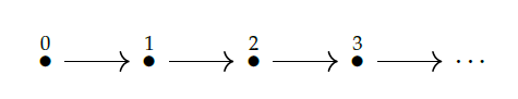 31 |
32 | Totally ordered sets are limiting. Suppose you're trying to order
33 | foods on a restaurant menu based on how much you like them. What's
34 | better: a cheese sandwich or a pancake? There may be no answer,
35 | because you like them in _different ways_. To get a totally ordered
36 | set you have to ignore this and arrange all the foods in a line.
37 |
38 | In standard economics we _do_ try to arrange everything in a line. We
39 | measure the worth of everything in real numbers: numbers of _dollars_.
40 | There's even a theorem to justify this, proved by [von Neumann and
41 | Morgenstern](https://en.wikipedia.org/wiki/Von_Neumann%E2%80%93Morgenstern_utility_theorem).
42 | But the assumptions of this theorem don't hold in real life. It's
43 | mainly just _convenient_ to measure value, or "utility", in real
44 | numbers. With computer technologies we could set up cryptocurrencies
45 | based on other posets. But will we?
46 |
47 | Luckily, human thought as a whole is not limited to total orders. A
48 | good example is logic. Logic, in its simplest form, is about
49 | statements \\(P, Q, R, \dots \\) and whether one statement implies
50 | another. If \\(P\\) implies \\(Q\\) we often write \\(P \implies
51 | Q\\). There are many kinds of logic, but every kind I know, this
52 | relation \\(\implies\\) makes statements into a preorder, since we
53 | have
54 |
55 | 1) reflexivity: \\(P \implies P\\)
56 |
57 | 2) transitivity: if \\(P \implies Q\\) and \\( Q \implies R \\) then
58 | \\(P \implies R\\).
59 |
60 | Often people make this preorder into a poset by imposing this rule:
61 |
62 | 3) antisymmetry: if \\(P \implies Q\\) and \\(Q \implies P\\) then
63 | \\(P = Q\\).
64 |
65 | This amounts to decreeing that we count two statements as "the same"
66 | if they both imply each other. We may not always want to do this.
67 | And we certainly don't want a linear order: it's easy to find examples
68 | of statements such that neither \\(P \implies Q\\) nor \\(Q \implies
69 | P\\), like "I am a millionaire" and "I am happy", or "I like this food
70 | for breakfast" and "I like this food for lunch".
71 |
72 | So, to continue our study of preorders, posets, monotone functions and
73 | Galois connections, we'll turn to logic! Category-theoretic logic is
74 | an enormous wonderful field, but we'll just do a bit of logic based on
75 | the poset of subsets of a set, followed by a bit of logic based on the
76 | poset of partitions of a set. The latter underlies Fong and Spivak's
77 | discussion of "generative effects" in Chapter 1.
78 |
79 | **[To read other lectures go here.](http://www.azimuthproject.org/azimuth/show/Applied+Category+Theory#Course)**
80 |
81 | ---
82 |
83 | [Click here to read the original discussion.](https://forum.azimuthproject.org/discussion/1909/lecture-7-chapter-1-logic/p1)
84 |
85 | ---
86 |
87 | {% include "../LICENSE.md" %}
88 |
--------------------------------------------------------------------------------
/chapter_1/lecture_5.md:
--------------------------------------------------------------------------------
1 | # Lecture 5 - Galois Connections Part 2
2 |
3 | ---
4 |
5 | Okay: I've told you what a Galois connection is. But now it's time to
6 | explain why they matter. This will take much longer - and be much more
7 | fun.
8 |
9 | Galois connections do something really cool: they tell you _the best
10 | possible way to recover data that can't be recovered_.
11 |
12 | More precisely, they tell you _the best approximation to reversing a
13 | computation that can't be reversed._
14 |
15 | Someone hands you the output of some computation, and asks you what
16 | the input was. Sometimes there's a unique right answer. But sometimes
17 | there's more than one answer, or none! That's when your job gets
18 | hard. In fact, impossible! But don't let that stop you.
19 |
20 |
31 |
32 | Totally ordered sets are limiting. Suppose you're trying to order
33 | foods on a restaurant menu based on how much you like them. What's
34 | better: a cheese sandwich or a pancake? There may be no answer,
35 | because you like them in _different ways_. To get a totally ordered
36 | set you have to ignore this and arrange all the foods in a line.
37 |
38 | In standard economics we _do_ try to arrange everything in a line. We
39 | measure the worth of everything in real numbers: numbers of _dollars_.
40 | There's even a theorem to justify this, proved by [von Neumann and
41 | Morgenstern](https://en.wikipedia.org/wiki/Von_Neumann%E2%80%93Morgenstern_utility_theorem).
42 | But the assumptions of this theorem don't hold in real life. It's
43 | mainly just _convenient_ to measure value, or "utility", in real
44 | numbers. With computer technologies we could set up cryptocurrencies
45 | based on other posets. But will we?
46 |
47 | Luckily, human thought as a whole is not limited to total orders. A
48 | good example is logic. Logic, in its simplest form, is about
49 | statements \\(P, Q, R, \dots \\) and whether one statement implies
50 | another. If \\(P\\) implies \\(Q\\) we often write \\(P \implies
51 | Q\\). There are many kinds of logic, but every kind I know, this
52 | relation \\(\implies\\) makes statements into a preorder, since we
53 | have
54 |
55 | 1) reflexivity: \\(P \implies P\\)
56 |
57 | 2) transitivity: if \\(P \implies Q\\) and \\( Q \implies R \\) then
58 | \\(P \implies R\\).
59 |
60 | Often people make this preorder into a poset by imposing this rule:
61 |
62 | 3) antisymmetry: if \\(P \implies Q\\) and \\(Q \implies P\\) then
63 | \\(P = Q\\).
64 |
65 | This amounts to decreeing that we count two statements as "the same"
66 | if they both imply each other. We may not always want to do this.
67 | And we certainly don't want a linear order: it's easy to find examples
68 | of statements such that neither \\(P \implies Q\\) nor \\(Q \implies
69 | P\\), like "I am a millionaire" and "I am happy", or "I like this food
70 | for breakfast" and "I like this food for lunch".
71 |
72 | So, to continue our study of preorders, posets, monotone functions and
73 | Galois connections, we'll turn to logic! Category-theoretic logic is
74 | an enormous wonderful field, but we'll just do a bit of logic based on
75 | the poset of subsets of a set, followed by a bit of logic based on the
76 | poset of partitions of a set. The latter underlies Fong and Spivak's
77 | discussion of "generative effects" in Chapter 1.
78 |
79 | **[To read other lectures go here.](http://www.azimuthproject.org/azimuth/show/Applied+Category+Theory#Course)**
80 |
81 | ---
82 |
83 | [Click here to read the original discussion.](https://forum.azimuthproject.org/discussion/1909/lecture-7-chapter-1-logic/p1)
84 |
85 | ---
86 |
87 | {% include "../LICENSE.md" %}
88 |
--------------------------------------------------------------------------------
/chapter_1/lecture_5.md:
--------------------------------------------------------------------------------
1 | # Lecture 5 - Galois Connections Part 2
2 |
3 | ---
4 |
5 | Okay: I've told you what a Galois connection is. But now it's time to
6 | explain why they matter. This will take much longer - and be much more
7 | fun.
8 |
9 | Galois connections do something really cool: they tell you _the best
10 | possible way to recover data that can't be recovered_.
11 |
12 | More precisely, they tell you _the best approximation to reversing a
13 | computation that can't be reversed._
14 |
15 | Someone hands you the output of some computation, and asks you what
16 | the input was. Sometimes there's a unique right answer. But sometimes
17 | there's more than one answer, or none! That's when your job gets
18 | hard. In fact, impossible! But don't let that stop you.
19 |
20 |  22 |
23 | Suppose we have a function between sets, \\(f : A \to B\\). We say a
24 | function \\(g: B \to A\\) is the **inverse** of \\(f\\) if
25 |
26 | \\[g(f(a)) = a \textrm{ for all } a \in A \quad \textrm{ and } \quad f(g(b)) = b \textrm{ for all } b \in B\\]
27 |
28 | Another equivalent way to say this is that
29 |
30 | \\[f(a) = b \textrm{ if and only if } a = g(b)\\]
31 |
32 | for all \\(a \in A\\) and \\(b \in B\\).
33 |
34 | So, the idea is that \\(g\\) undoes \\(f\\). For example, if \\(A = B
35 | = \mathbb{R}\\) is the set of real numbers, and \\(f\\) doubles every
36 | number, then \\(f\\) has an inverse \\(g\\), which halves every
37 | number.
38 |
39 | But what if \\(A = B = \mathbb{N}\\) is the set of _natural_ numbers,
40 | and \\(f\\) doubles every natural number. This function has no
41 | inverse!
42 |
43 | So, if I say "\\(2a = 4\\); tell me \\(a\\)" you can say \\(a = 2\\).
44 | But if I say "\\(2a = 3\\); tell me \\(a\\)" you're stuck.
45 |
46 | But you can still try to give me a "best approximation" to the
47 | nonexistent natural number \\(a\\) with \\(2 a = 3\\).
48 |
49 | "Best" in what sense? We could look for the number \\(a\\) that makes
50 | \\(2a\\) as close as possible to 3. There are two equally good
51 | options: \\(a = 1\\) and \\(a = 2\\). Here we are using the usual
52 | distance function, or
53 | [metric](https://en.wikipedia.org/wiki/Metric_(mathematics)), on
54 | \\(\mathbb{N}\\), which says that the distance between \\(x\\) and
55 | \\(y\\) is \\(|x-y|\\).
56 |
57 | But we're not talking about distance functions in this class now!
58 | We're talking about _preorders_. Can we define a "best approximation"
59 | using just the relation \\(\le\\) on \\(\mathbb{N}\\)?
60 |
61 | Yes! But we can do it in two ways!
62 |
63 | **Best approximation from below.** Find the largest possible \\(a \in
64 | \mathbb{N}\\) such that \\(2a \le 3\\). Answer: \\(a = 1\\).
65 |
66 | **Best approximation from above.** Find the smallest possible \\(a \in
67 | \mathbb{N}\\) such that \\(3 \le 2a\\). Answer: \\(a = 2\\).
68 |
69 | Okay, now work this out more generally:
70 |
71 | **Puzzle 14.** Find the function \\(g : \mathbb{N} \to \mathbb{N}\\)
72 | such that \\(g(b) \\) is the largest possible natural number \\(a\\)
73 | with \\(2a \le b\\).
74 |
75 | **Puzzle 15.** Find the function \\(g : \mathbb{N} \to \mathbb{N}\\)
76 | such that \\(g(b)\\) is the smallest possible natural number \\(a\\)
77 | with \\(b \le 2a\\).
78 |
79 | Now think about [Lecture 4](lecture_4.md) and the puzzles there! I'll
80 | copy them here with notation that better matches what I'm using now:
81 |
82 | **Puzzle 12.** Find a right adjoint for the function \\(f: \mathbb{N}
83 | \to \mathbb{N}\\) that doubles natural numbers: that is, a function
84 | \\(g : \mathbb{N} \to \mathbb{N}\\) with
85 |
86 | \\[f(a) \le b \textrm{ if and only if } a \le g(b)\\]
87 |
88 | for all \\(a,b \in \mathbb{N}\\).
89 |
90 | **Puzzle 13.** Find a left adjoint for the same function \\(f\\): that
91 | is, a function \\(g : \mathbb{N} \to \mathbb{N}\\) with
92 |
93 | \\[g(b) \le a \textrm{ if and only if } b \le f(a)\\]
94 |
95 | Next:
96 |
97 | **Puzzle 16.** What's going on here? What's the pattern you see, and
98 | why is it working this way?
99 |
100 | **[To read other lectures go here.](http://www.azimuthproject.org/azimuth/show/Applied+Category+Theory#Course)**
101 |
102 | ---
103 |
104 | [Click here to read the original
105 | discussion](https://forum.azimuthproject.org/discussion/1845/lecture-5-chapter-1-galois-connections/p1)
106 |
107 | ---
108 |
109 | {% include "../LICENSE.md" %}
110 |
--------------------------------------------------------------------------------
/chapter_1/lecture_6.md:
--------------------------------------------------------------------------------
1 | # Lecture 6 - Computing Adjoints
2 | ---
3 | I've already said that left and right adjoints give _the best
4 | approximate ways to solve a problem that has no solution_, namely
5 | finding the inverse of a monotone function that has no inverse. I've
6 | defined them and given you some puzzles about them. But now let's
7 | review these puzzles and extract some valuable lessons!
8 |
9 | We took the function \\(f : \mathbb{N} \to \mathbb{N}\\) that doubles
10 | any natural number
11 |
12 | \\[f(a) = 2a .\\]
13 |
14 | This function has no inverse, since you can't divide an odd number by
15 | 2 and get a natural number! But if you did the puzzles, you saw that
16 | \\(f\\) has a "right adjoint" \\(g : \mathbb{N} \to \mathbb{N}\\).
17 | This is defined by the property
18 |
19 | \\[f(a) \le b \textrm{ if and only if } a \le g(b) .\\]
20 |
21 | or in other words,
22 |
23 | \\[2a \le b \textrm{ if and only if } a \le g(b) .\\]
24 |
25 | Using our knowledge of fractions, we have
26 |
27 | \\[2a \le b \textrm{ if and only if } a \le b/2\\]
28 |
29 | but since \\(a\\) is a natural number, this implies
30 |
31 | \\[2a \le b \textrm{ if and only if } a \le \lfloor b/2 \rfloor\\]
32 |
33 | where we are using the [floor
34 | function](https://en.wikipedia.org/wiki/Floor_and_ceiling_functions)
35 | to pick out the largest integer \\(\le b/2\\). So,
36 |
37 | \\[g(b) = \lfloor b/2 \rfloor.\\]
38 |
39 | Moral: the right adjoint \\(g\\) is the "best approximation from
40 | below" to the nonexistent inverse of \\(f\\).
41 |
42 | If you did the puzzles, you also saw that \\(f\\) has a left adjoint!
43 | This is the "best approximation from above" to the nonexistent inverse
44 | of \\(f\\): it gives you the smallest integer that's \\(\ge n/2\\).
45 |
46 | So, while \\(f\\) has no inverse, it has two "approximate inverses".
47 | The left adjoint comes as close as possible to the (perhaps
48 | nonexistent) correct answer while making sure to never choose a number
49 | that's _too small_. The right adjoint comes as close as possible while
50 | making sure to never choose a number that's _too big_.
51 |
52 | The two adjoints represent two opposing philosophies of life: _make
53 | sure you never ask for too little_ and _make sure you never ask for
54 | too much_. This is why they're philosophically profound. But the great
55 | thing is that they are defined in a completely precise, systematic way
56 | that applies to a huge number of situations!
57 |
58 | If you need a mnemonic to remember which is which, remember left
59 | adjoints are "left-wing" or "liberal" or "generous", while right
60 | adjoints are "right-wing" or "conservative" or "cautious".
61 |
62 | Let's think a bit more about how we can compute them in general,
63 | starting from the basic definition.
64 |
65 | Here's the definition again. Suppose we have two preorders
66 | \\((A,\le_A)\\) and \\((B,\le_B)\\) and a monotone function \\(f : A
67 | \to B\\). Then we say a monotone function \\(g: B \to A\\) is a
68 | **right adjoint of \\(f\\)** if
69 |
70 | \\[f(a) \le_B b \textrm{ if and only if } a \le_A g(b)\\]
71 |
72 | for all \\(a \in A\\) and \\(b \in B\\). In this situation we also say
73 | that \\(f\\) is a **left adjoint of \\(g\\)**.
74 |
75 | The names should be easy to remember, since \\(f\\) shows up on the
76 | _left_ of the inequality $$f(a) \le_B b$$, while \\(g\\) shows up on
77 | the _right_ of the inequality \\(a \le_A g(b)\\). But let's see how
78 | they actually work!
79 |
80 | Suppose you know \\(f : A \to B\\) and you're trying to figure out its
81 | right adjoint \\(g: B \to A\\). Say you're trying to figure out
82 | \\(g(b)\\). You don't know what it is, but you know
83 |
84 | \\[f(a) \le_B b \textrm{ if and only if } a \le_A g(b)\\]
85 |
86 | So, you go around looking at choices of \\(a \in A\\). For each one
87 | you compute \\(f(a)\\). If \\(f(a) \le_B b\\), then you know \\(a
88 | \le_A g(b)\\). So, you need to choose \\(g(b)\\) to be greater than or
89 | equal to every element of this set:
90 |
91 | \\[\{a \in A : \; f(a) \le_B b \}\\]
92 |
93 | In other words, \\(g(b)\\) must be an **[upper
94 | bound](https://en.wikipedia.org/wiki/Upper_and_lower_bounds)** of this
95 | set. But you shouldn't choose \\(g(b)\\) to be any bigger than it
96 | needs to be! After all, you know $$a \le_A g(b)$$ _only if_ $$f(a)
97 | \le_B b$$. So, \\(g(b)\\) must be a **[least upper
98 | bound](https://en.wikipedia.org/wiki/Infimum_and_supremum)** of the
99 | above set.
100 |
101 | Note that I'm carefully speaking about _a_ least upper bound. Our set
102 | could have two different least upper bounds, say \\(a\\) and \\(a'\\).
103 | Since they're both the least, we must have \\(a \le a'\\) and \\(a'
104 | \le a\\). This doesn't imply \\(a = a'\\), in general! But it does if
105 | our preorder \\(A\\) is a "poset". A **poset** is a preorder \\((A,
106 | \le_A)\\) obeying this extra axiom:
107 |
108 | \\[\textrm{ if } a \le a' \textrm{ and } a' \le a \textrm{ then } a = a'\\]
109 |
110 | for all \\(a,a' \in A\\).
111 |
112 | In a poset, our desired least upper bound may still not _exist_. But
113 | if it does, it's _unique_, and Fong and Spivak write it this way:
114 |
115 | \\[\bigvee \{a \in A : \; f(a) \le_B b \}\\]
116 |
117 | The \\(\bigvee\\) symbol stands for "least upper bound", also known as
118 | **supremum** or **join**.
119 |
120 | So, here's what we've shown:
121 |
122 | If \\(f : A \to B\\) has a right adjoint \\(g : B \to A\\) and \\(A\\)
123 | is a poset, this right adjoint is unique and we have a formula for it:
124 |
125 | \\[g(b) = \bigvee \{a \in A : \; f(a) \le_B b \} .\\]
126 |
127 | And we can copy our whole line of reasoning and show this:
128 |
129 | If \\(g : B \to A\\) has a left adjoint \\(f : A \to B\\) and \\(B\\)
130 | is a poset, this left adjoint is unique and we have a formula for it:
131 |
132 | \\[f(a) = \bigwedge \{b \in B : \; a \le_A g(b)\}.\\]
133 |
134 | Here the \\(\bigwedge\\) symbol stands for "greatest lower bound",
135 | also known as the **infimum** or **meet**.
136 |
137 | We're making progress: we can now actually compute left and right
138 | adjoints! Next we'll start looking at more examples.
139 |
140 | **[To read other lectures go here.](http://www.azimuthproject.org/azimuth/show/Applied+Category+Theory#Course)**
141 |
142 | ---
143 |
144 | [Click here to read the original discussion.](https://forum.azimuthproject.org/discussion/1901/lecture-6-chapter-1-computing-adjoints/p1)
145 |
146 | ---
147 |
148 | {% include "../LICENSE.md" %}
149 |
--------------------------------------------------------------------------------
/chapter_1/lecture_10.md:
--------------------------------------------------------------------------------
1 | # Lecture 10 - The Logic of Partitions
2 |
3 | ---
4 |
5 | I've been explaining how we can create a version of logic starting
6 | from any poset, which we think of as a poset of "propositions". There
7 | are various ways to get our hands on such a poset. One way is to start
8 | with a set \\(X\\) and build a poset \\(P(X)\\) whose elements are
9 | subsets of \\(X\\). This leads to the most traditional form of logic,
10 | called classical logic. But another way is to start with a set \\(X\\)
11 | and build a poset \\(\mathcal{E}(X)\\) whose elements are "partitions"
12 | of \\(X\\). This leads to another form of logic, called the logic of
13 | partitions.
14 |
15 | What's a partition? It's a way of chopping the set \\(X\\) into
16 | "parts". We want each part to be a nonempty subset of \\(X\\), we want
17 | these parts to be disjoint, and we want their union to be all of
18 | \\(X\\). For example, here are all 52 partitions of a set with 5
19 | elements:
20 |
21 |
22 |
23 | Suppose we have a function between sets, \\(f : A \to B\\). We say a
24 | function \\(g: B \to A\\) is the **inverse** of \\(f\\) if
25 |
26 | \\[g(f(a)) = a \textrm{ for all } a \in A \quad \textrm{ and } \quad f(g(b)) = b \textrm{ for all } b \in B\\]
27 |
28 | Another equivalent way to say this is that
29 |
30 | \\[f(a) = b \textrm{ if and only if } a = g(b)\\]
31 |
32 | for all \\(a \in A\\) and \\(b \in B\\).
33 |
34 | So, the idea is that \\(g\\) undoes \\(f\\). For example, if \\(A = B
35 | = \mathbb{R}\\) is the set of real numbers, and \\(f\\) doubles every
36 | number, then \\(f\\) has an inverse \\(g\\), which halves every
37 | number.
38 |
39 | But what if \\(A = B = \mathbb{N}\\) is the set of _natural_ numbers,
40 | and \\(f\\) doubles every natural number. This function has no
41 | inverse!
42 |
43 | So, if I say "\\(2a = 4\\); tell me \\(a\\)" you can say \\(a = 2\\).
44 | But if I say "\\(2a = 3\\); tell me \\(a\\)" you're stuck.
45 |
46 | But you can still try to give me a "best approximation" to the
47 | nonexistent natural number \\(a\\) with \\(2 a = 3\\).
48 |
49 | "Best" in what sense? We could look for the number \\(a\\) that makes
50 | \\(2a\\) as close as possible to 3. There are two equally good
51 | options: \\(a = 1\\) and \\(a = 2\\). Here we are using the usual
52 | distance function, or
53 | [metric](https://en.wikipedia.org/wiki/Metric_(mathematics)), on
54 | \\(\mathbb{N}\\), which says that the distance between \\(x\\) and
55 | \\(y\\) is \\(|x-y|\\).
56 |
57 | But we're not talking about distance functions in this class now!
58 | We're talking about _preorders_. Can we define a "best approximation"
59 | using just the relation \\(\le\\) on \\(\mathbb{N}\\)?
60 |
61 | Yes! But we can do it in two ways!
62 |
63 | **Best approximation from below.** Find the largest possible \\(a \in
64 | \mathbb{N}\\) such that \\(2a \le 3\\). Answer: \\(a = 1\\).
65 |
66 | **Best approximation from above.** Find the smallest possible \\(a \in
67 | \mathbb{N}\\) such that \\(3 \le 2a\\). Answer: \\(a = 2\\).
68 |
69 | Okay, now work this out more generally:
70 |
71 | **Puzzle 14.** Find the function \\(g : \mathbb{N} \to \mathbb{N}\\)
72 | such that \\(g(b) \\) is the largest possible natural number \\(a\\)
73 | with \\(2a \le b\\).
74 |
75 | **Puzzle 15.** Find the function \\(g : \mathbb{N} \to \mathbb{N}\\)
76 | such that \\(g(b)\\) is the smallest possible natural number \\(a\\)
77 | with \\(b \le 2a\\).
78 |
79 | Now think about [Lecture 4](lecture_4.md) and the puzzles there! I'll
80 | copy them here with notation that better matches what I'm using now:
81 |
82 | **Puzzle 12.** Find a right adjoint for the function \\(f: \mathbb{N}
83 | \to \mathbb{N}\\) that doubles natural numbers: that is, a function
84 | \\(g : \mathbb{N} \to \mathbb{N}\\) with
85 |
86 | \\[f(a) \le b \textrm{ if and only if } a \le g(b)\\]
87 |
88 | for all \\(a,b \in \mathbb{N}\\).
89 |
90 | **Puzzle 13.** Find a left adjoint for the same function \\(f\\): that
91 | is, a function \\(g : \mathbb{N} \to \mathbb{N}\\) with
92 |
93 | \\[g(b) \le a \textrm{ if and only if } b \le f(a)\\]
94 |
95 | Next:
96 |
97 | **Puzzle 16.** What's going on here? What's the pattern you see, and
98 | why is it working this way?
99 |
100 | **[To read other lectures go here.](http://www.azimuthproject.org/azimuth/show/Applied+Category+Theory#Course)**
101 |
102 | ---
103 |
104 | [Click here to read the original
105 | discussion](https://forum.azimuthproject.org/discussion/1845/lecture-5-chapter-1-galois-connections/p1)
106 |
107 | ---
108 |
109 | {% include "../LICENSE.md" %}
110 |
--------------------------------------------------------------------------------
/chapter_1/lecture_6.md:
--------------------------------------------------------------------------------
1 | # Lecture 6 - Computing Adjoints
2 | ---
3 | I've already said that left and right adjoints give _the best
4 | approximate ways to solve a problem that has no solution_, namely
5 | finding the inverse of a monotone function that has no inverse. I've
6 | defined them and given you some puzzles about them. But now let's
7 | review these puzzles and extract some valuable lessons!
8 |
9 | We took the function \\(f : \mathbb{N} \to \mathbb{N}\\) that doubles
10 | any natural number
11 |
12 | \\[f(a) = 2a .\\]
13 |
14 | This function has no inverse, since you can't divide an odd number by
15 | 2 and get a natural number! But if you did the puzzles, you saw that
16 | \\(f\\) has a "right adjoint" \\(g : \mathbb{N} \to \mathbb{N}\\).
17 | This is defined by the property
18 |
19 | \\[f(a) \le b \textrm{ if and only if } a \le g(b) .\\]
20 |
21 | or in other words,
22 |
23 | \\[2a \le b \textrm{ if and only if } a \le g(b) .\\]
24 |
25 | Using our knowledge of fractions, we have
26 |
27 | \\[2a \le b \textrm{ if and only if } a \le b/2\\]
28 |
29 | but since \\(a\\) is a natural number, this implies
30 |
31 | \\[2a \le b \textrm{ if and only if } a \le \lfloor b/2 \rfloor\\]
32 |
33 | where we are using the [floor
34 | function](https://en.wikipedia.org/wiki/Floor_and_ceiling_functions)
35 | to pick out the largest integer \\(\le b/2\\). So,
36 |
37 | \\[g(b) = \lfloor b/2 \rfloor.\\]
38 |
39 | Moral: the right adjoint \\(g\\) is the "best approximation from
40 | below" to the nonexistent inverse of \\(f\\).
41 |
42 | If you did the puzzles, you also saw that \\(f\\) has a left adjoint!
43 | This is the "best approximation from above" to the nonexistent inverse
44 | of \\(f\\): it gives you the smallest integer that's \\(\ge n/2\\).
45 |
46 | So, while \\(f\\) has no inverse, it has two "approximate inverses".
47 | The left adjoint comes as close as possible to the (perhaps
48 | nonexistent) correct answer while making sure to never choose a number
49 | that's _too small_. The right adjoint comes as close as possible while
50 | making sure to never choose a number that's _too big_.
51 |
52 | The two adjoints represent two opposing philosophies of life: _make
53 | sure you never ask for too little_ and _make sure you never ask for
54 | too much_. This is why they're philosophically profound. But the great
55 | thing is that they are defined in a completely precise, systematic way
56 | that applies to a huge number of situations!
57 |
58 | If you need a mnemonic to remember which is which, remember left
59 | adjoints are "left-wing" or "liberal" or "generous", while right
60 | adjoints are "right-wing" or "conservative" or "cautious".
61 |
62 | Let's think a bit more about how we can compute them in general,
63 | starting from the basic definition.
64 |
65 | Here's the definition again. Suppose we have two preorders
66 | \\((A,\le_A)\\) and \\((B,\le_B)\\) and a monotone function \\(f : A
67 | \to B\\). Then we say a monotone function \\(g: B \to A\\) is a
68 | **right adjoint of \\(f\\)** if
69 |
70 | \\[f(a) \le_B b \textrm{ if and only if } a \le_A g(b)\\]
71 |
72 | for all \\(a \in A\\) and \\(b \in B\\). In this situation we also say
73 | that \\(f\\) is a **left adjoint of \\(g\\)**.
74 |
75 | The names should be easy to remember, since \\(f\\) shows up on the
76 | _left_ of the inequality $$f(a) \le_B b$$, while \\(g\\) shows up on
77 | the _right_ of the inequality \\(a \le_A g(b)\\). But let's see how
78 | they actually work!
79 |
80 | Suppose you know \\(f : A \to B\\) and you're trying to figure out its
81 | right adjoint \\(g: B \to A\\). Say you're trying to figure out
82 | \\(g(b)\\). You don't know what it is, but you know
83 |
84 | \\[f(a) \le_B b \textrm{ if and only if } a \le_A g(b)\\]
85 |
86 | So, you go around looking at choices of \\(a \in A\\). For each one
87 | you compute \\(f(a)\\). If \\(f(a) \le_B b\\), then you know \\(a
88 | \le_A g(b)\\). So, you need to choose \\(g(b)\\) to be greater than or
89 | equal to every element of this set:
90 |
91 | \\[\{a \in A : \; f(a) \le_B b \}\\]
92 |
93 | In other words, \\(g(b)\\) must be an **[upper
94 | bound](https://en.wikipedia.org/wiki/Upper_and_lower_bounds)** of this
95 | set. But you shouldn't choose \\(g(b)\\) to be any bigger than it
96 | needs to be! After all, you know $$a \le_A g(b)$$ _only if_ $$f(a)
97 | \le_B b$$. So, \\(g(b)\\) must be a **[least upper
98 | bound](https://en.wikipedia.org/wiki/Infimum_and_supremum)** of the
99 | above set.
100 |
101 | Note that I'm carefully speaking about _a_ least upper bound. Our set
102 | could have two different least upper bounds, say \\(a\\) and \\(a'\\).
103 | Since they're both the least, we must have \\(a \le a'\\) and \\(a'
104 | \le a\\). This doesn't imply \\(a = a'\\), in general! But it does if
105 | our preorder \\(A\\) is a "poset". A **poset** is a preorder \\((A,
106 | \le_A)\\) obeying this extra axiom:
107 |
108 | \\[\textrm{ if } a \le a' \textrm{ and } a' \le a \textrm{ then } a = a'\\]
109 |
110 | for all \\(a,a' \in A\\).
111 |
112 | In a poset, our desired least upper bound may still not _exist_. But
113 | if it does, it's _unique_, and Fong and Spivak write it this way:
114 |
115 | \\[\bigvee \{a \in A : \; f(a) \le_B b \}\\]
116 |
117 | The \\(\bigvee\\) symbol stands for "least upper bound", also known as
118 | **supremum** or **join**.
119 |
120 | So, here's what we've shown:
121 |
122 | If \\(f : A \to B\\) has a right adjoint \\(g : B \to A\\) and \\(A\\)
123 | is a poset, this right adjoint is unique and we have a formula for it:
124 |
125 | \\[g(b) = \bigvee \{a \in A : \; f(a) \le_B b \} .\\]
126 |
127 | And we can copy our whole line of reasoning and show this:
128 |
129 | If \\(g : B \to A\\) has a left adjoint \\(f : A \to B\\) and \\(B\\)
130 | is a poset, this left adjoint is unique and we have a formula for it:
131 |
132 | \\[f(a) = \bigwedge \{b \in B : \; a \le_A g(b)\}.\\]
133 |
134 | Here the \\(\bigwedge\\) symbol stands for "greatest lower bound",
135 | also known as the **infimum** or **meet**.
136 |
137 | We're making progress: we can now actually compute left and right
138 | adjoints! Next we'll start looking at more examples.
139 |
140 | **[To read other lectures go here.](http://www.azimuthproject.org/azimuth/show/Applied+Category+Theory#Course)**
141 |
142 | ---
143 |
144 | [Click here to read the original discussion.](https://forum.azimuthproject.org/discussion/1901/lecture-6-chapter-1-computing-adjoints/p1)
145 |
146 | ---
147 |
148 | {% include "../LICENSE.md" %}
149 |
--------------------------------------------------------------------------------
/chapter_1/lecture_10.md:
--------------------------------------------------------------------------------
1 | # Lecture 10 - The Logic of Partitions
2 |
3 | ---
4 |
5 | I've been explaining how we can create a version of logic starting
6 | from any poset, which we think of as a poset of "propositions". There
7 | are various ways to get our hands on such a poset. One way is to start
8 | with a set \\(X\\) and build a poset \\(P(X)\\) whose elements are
9 | subsets of \\(X\\). This leads to the most traditional form of logic,
10 | called classical logic. But another way is to start with a set \\(X\\)
11 | and build a poset \\(\mathcal{E}(X)\\) whose elements are "partitions"
12 | of \\(X\\). This leads to another form of logic, called the logic of
13 | partitions.
14 |
15 | What's a partition? It's a way of chopping the set \\(X\\) into
16 | "parts". We want each part to be a nonempty subset of \\(X\\), we want
17 | these parts to be disjoint, and we want their union to be all of
18 | \\(X\\). For example, here are all 52 partitions of a set with 5
19 | elements:
20 |
21 | 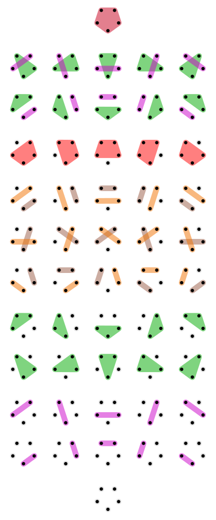 22 |
23 | At the top we see the "coarsest" partition, where all 5 elements are
24 | in the same part. At the bottom we see the "finest" partition, where
25 | each element is in its own separate part.
26 |
27 | How can we think of these partitions as "propositions"? Here's how:
28 | each partition gives a proposition saying that two elements in the
29 | same part are "equivalent", or the same in some way. The coarser the
30 | partition, the more elements are equivalent.
31 |
32 | For example, imagine you're a detective trying to solve a case on a
33 | small island with 5 people on it. At first you don't know any of them
34 | are related, so they're all in separate families, as far as you know:
35 |
36 |
22 |
23 | At the top we see the "coarsest" partition, where all 5 elements are
24 | in the same part. At the bottom we see the "finest" partition, where
25 | each element is in its own separate part.
26 |
27 | How can we think of these partitions as "propositions"? Here's how:
28 | each partition gives a proposition saying that two elements in the
29 | same part are "equivalent", or the same in some way. The coarser the
30 | partition, the more elements are equivalent.
31 |
32 | For example, imagine you're a detective trying to solve a case on a
33 | small island with 5 people on it. At first you don't know any of them
34 | are related, so they're all in separate families, as far as you know:
35 |
36 |  37 |
38 | But then you start digging into their history. Each time you learn
39 | that two people are related, you change your partition by putting them
40 | into the same part:
41 |
42 |
37 |
38 | But then you start digging into their history. Each time you learn
39 | that two people are related, you change your partition by putting them
40 | into the same part:
41 |
42 |  43 |
44 | You keep doing this as secret family relationships are revealed:
45 |
46 |
43 |
44 | You keep doing this as secret family relationships are revealed:
45 |
46 |  47 |
48 | In this example, as you learn more you move to _coarser_ partitions,
49 | because your goal is to find relationships between people, and lump
50 | them in as big bunches as possible. But often people think about
51 | partition logic a bit differently, where as you learn more you move to
52 | _finer_ partitions.
53 |
54 | Suppose you are an amateur wine taster learning to distinguish
55 | different kinds of wine by their taste. At first all wines taste
56 | alike, so they're all lumped together:
57 |
58 |
47 |
48 | In this example, as you learn more you move to _coarser_ partitions,
49 | because your goal is to find relationships between people, and lump
50 | them in as big bunches as possible. But often people think about
51 | partition logic a bit differently, where as you learn more you move to
52 | _finer_ partitions.
53 |
54 | Suppose you are an amateur wine taster learning to distinguish
55 | different kinds of wine by their taste. At first all wines taste
56 | alike, so they're all lumped together:
57 |
58 |  59 |
60 | When you learn to distinguish red and white wines, you move to a finer
61 | partition:
62 |
63 |
59 |
60 | When you learn to distinguish red and white wines, you move to a finer
61 | partition:
62 |
63 |  64 |
65 | This sort of example will fit our story a bit better. We'll generally
66 | say that you know more if your partition is _finer_.
67 |
68 | Now it's time to define partitions more carefully! A partition of
69 | \\(X\\) is a bunch of subsets of \\(X\\). So, it's a subset of
70 | \\(P(X)\\). Please think about that until it makes sense, or ask
71 | questions. There are a lot of sets and subsets running around: it can
72 | be confusing. But here we go:
73 |
74 | **Definition.** A **partition** of a set \\(X\\) is a set \\(P
75 | \subseteq P(X)\\) such that:
76 |
77 | 1. Each set \\(S \in P\\) is nonempty.
78 |
79 | 2. Distinct sets \\(S, T \in P\\) are disjoint: that is, if \\(S \ne
80 | T\\) then \\(S \cap T = \emptyset\\).
81 |
82 | 3. The union of all the sets \\(S \in P\\) is \\(X\\): that is,
83 |
84 | \\[X = \bigcup_{S \in P} S.\\]
85 |
86 | We call the sets \\(S \in P\\) the **parts** of the partition.
87 |
88 | I said that each partition \\(P\\) gives an equivalence relation,
89 | where two elements of \\(X\\) are "equivalent" if and only if they're
90 | in the same part. Let's make that precise too:
91 |
92 | **Definition.** An **equivalence relation** on a set \\(X\\) is a
93 | relation \\(\sim\\) on \\(X\\) that is:
94 |
95 | 1. **Reflexive:** for all \\(x \in X\\), \\(x \sim x\\).
96 |
97 | 2. **Transitive:** for all \\(x,y,z \in Z\\), \\(x \sim y\\) and \\(y
98 | \sim z\\) imply \\(x \sim z\\).
99 |
100 | 3. **Symmetric:** for all \\(x,y \in X\\), \\(x \sim y\\) implies \\(y
101 | \sim x.\\)
102 |
103 | **Puzzle 28.** Show that if \\(P\\) is a partition of a set \\(X\\),
104 | and we define a relation \\(\sim_P\\) on \\(X\\) as follows:
105 |
106 | \\[x \sim_P y \textrm{ if and only if } x, y \in S \textrm{ for some } S \in P,\\]
107 |
108 | then \\(\sim_P\\) is an equivalence relation.
109 |
110 | **Puzzle 29.** Show that if \\(\sim\\) is an equivalence relation on a
111 | set \\(X\\), we can define a partition \\(P_\sim\\) on \\(X\\) whose
112 | parts are precisely the sets of the form
113 |
114 | \\[S_x = \\{y \in X : \; y \sim x \\}\\]
115 |
116 | with \\(x \in X\\). We call \\(S_x\\) the **equivalence class** of
117 | \\(x\\).
118 |
119 | **Puzzle 31.** Show that the previous two puzzles give a one-to-one
120 | correspondence between partitions of \\(X\\) and equivalence relations
121 | on \\(X\\).
122 |
123 | **Puzzle 32.** Proposition 1.11 of _[Seven
124 | Sketches](http://math.mit.edu/~dspivak/teaching/sp18/7Sketches.pdf)_
125 | asserts that there is a one-to-one correspondence between partitions
126 | of \\(X\\) and equivalence relations on \\(X\\). However, in the
127 | current version of the book this proposition is false! Nonetheless,
128 | the statement in Puzzle 31 is correct. How is this possible? (Hint:
129 | you have to read their definitions quite carefully. This is good
130 | practice in reading mathematics.)
131 |
132 | **Puzzle 33.** Is an equivalence relation always a preorder?
133 |
134 | **[To read other lectures go here.](http://www.azimuthproject.org/azimuth/show/Applied+Category+Theory#Course)**
135 |
136 | ---
137 |
138 | [Click here to read the original discussion.](https://forum.azimuthproject.org/discussion/1963/lecture-10-chapter-1-the-logic-of-partitions/p1)
139 |
140 | ---
141 |
142 | {% include "../LICENSE.md" %}
143 |
--------------------------------------------------------------------------------
/chapter_1/lecture_12.md:
--------------------------------------------------------------------------------
1 | # Lecture 12 - Generative Effects
2 |
3 | ---
4 |
5 | We now reach a topic highlighted by Fong and Spivak: "generative
6 | effects". These are, roughly, situations where the whole is more than
7 | the sum of its parts. A nice example shows up in the logic of
8 | partitions.
9 |
10 | Remember that any set \\(X\\) has a poset of partitions. This poset is
11 | called \\(\mathcal{E}(X)\\), and its elements are partitions of
12 | \\(X\\). Each partition \\(P\\) corresponds to an equivalence relation
13 | \\(\sim_P\\), where \\(x \sim_P y\\) if and only if \\(x\\) and
14 | \\(y\\) are in the same part of \\(P\\). This makes it easy to
15 | describe the partial order on \\(\mathcal{E}(X)\\): we say a partition
16 | \\(P\\) is **finer** than a partition \\(Q\\), or \\(Q\\) is
17 | **coarser** than \\(P\\), or simply \\(P \le Q\\), when
18 |
19 | \\[ x \sim_P y \textrm{ implies } x \sim_Q y \\]
20 |
21 | for all \\(x,y \in X\\).
22 |
23 | Now that we have this poset, how can we do _logic_ with it?
24 |
25 | In the logic of subsets, we've seen that "and" and "or" are the
26 | operations of "meet" and "join" in a certain poset. So, the logic of
27 | partitions should use "meet" and "join" in the poset
28 | \\(\mathcal{E}(X)\\). Let's see what they're like!
29 |
30 | First, we can ask whether two partitions \\(P\\) and \\(Q\\) have a
31 | meet. Remember: the **meet** \\(P \wedge Q\\), if it exists, is the
32 | coarsest partition that is finer than \\(P\\) and \\(Q\\).
33 |
34 | **Puzzle 34.** Can you draw the coarsest partition that's finer than
35 | these two partitions?
36 |
37 |
64 |
65 | This sort of example will fit our story a bit better. We'll generally
66 | say that you know more if your partition is _finer_.
67 |
68 | Now it's time to define partitions more carefully! A partition of
69 | \\(X\\) is a bunch of subsets of \\(X\\). So, it's a subset of
70 | \\(P(X)\\). Please think about that until it makes sense, or ask
71 | questions. There are a lot of sets and subsets running around: it can
72 | be confusing. But here we go:
73 |
74 | **Definition.** A **partition** of a set \\(X\\) is a set \\(P
75 | \subseteq P(X)\\) such that:
76 |
77 | 1. Each set \\(S \in P\\) is nonempty.
78 |
79 | 2. Distinct sets \\(S, T \in P\\) are disjoint: that is, if \\(S \ne
80 | T\\) then \\(S \cap T = \emptyset\\).
81 |
82 | 3. The union of all the sets \\(S \in P\\) is \\(X\\): that is,
83 |
84 | \\[X = \bigcup_{S \in P} S.\\]
85 |
86 | We call the sets \\(S \in P\\) the **parts** of the partition.
87 |
88 | I said that each partition \\(P\\) gives an equivalence relation,
89 | where two elements of \\(X\\) are "equivalent" if and only if they're
90 | in the same part. Let's make that precise too:
91 |
92 | **Definition.** An **equivalence relation** on a set \\(X\\) is a
93 | relation \\(\sim\\) on \\(X\\) that is:
94 |
95 | 1. **Reflexive:** for all \\(x \in X\\), \\(x \sim x\\).
96 |
97 | 2. **Transitive:** for all \\(x,y,z \in Z\\), \\(x \sim y\\) and \\(y
98 | \sim z\\) imply \\(x \sim z\\).
99 |
100 | 3. **Symmetric:** for all \\(x,y \in X\\), \\(x \sim y\\) implies \\(y
101 | \sim x.\\)
102 |
103 | **Puzzle 28.** Show that if \\(P\\) is a partition of a set \\(X\\),
104 | and we define a relation \\(\sim_P\\) on \\(X\\) as follows:
105 |
106 | \\[x \sim_P y \textrm{ if and only if } x, y \in S \textrm{ for some } S \in P,\\]
107 |
108 | then \\(\sim_P\\) is an equivalence relation.
109 |
110 | **Puzzle 29.** Show that if \\(\sim\\) is an equivalence relation on a
111 | set \\(X\\), we can define a partition \\(P_\sim\\) on \\(X\\) whose
112 | parts are precisely the sets of the form
113 |
114 | \\[S_x = \\{y \in X : \; y \sim x \\}\\]
115 |
116 | with \\(x \in X\\). We call \\(S_x\\) the **equivalence class** of
117 | \\(x\\).
118 |
119 | **Puzzle 31.** Show that the previous two puzzles give a one-to-one
120 | correspondence between partitions of \\(X\\) and equivalence relations
121 | on \\(X\\).
122 |
123 | **Puzzle 32.** Proposition 1.11 of _[Seven
124 | Sketches](http://math.mit.edu/~dspivak/teaching/sp18/7Sketches.pdf)_
125 | asserts that there is a one-to-one correspondence between partitions
126 | of \\(X\\) and equivalence relations on \\(X\\). However, in the
127 | current version of the book this proposition is false! Nonetheless,
128 | the statement in Puzzle 31 is correct. How is this possible? (Hint:
129 | you have to read their definitions quite carefully. This is good
130 | practice in reading mathematics.)
131 |
132 | **Puzzle 33.** Is an equivalence relation always a preorder?
133 |
134 | **[To read other lectures go here.](http://www.azimuthproject.org/azimuth/show/Applied+Category+Theory#Course)**
135 |
136 | ---
137 |
138 | [Click here to read the original discussion.](https://forum.azimuthproject.org/discussion/1963/lecture-10-chapter-1-the-logic-of-partitions/p1)
139 |
140 | ---
141 |
142 | {% include "../LICENSE.md" %}
143 |
--------------------------------------------------------------------------------
/chapter_1/lecture_12.md:
--------------------------------------------------------------------------------
1 | # Lecture 12 - Generative Effects
2 |
3 | ---
4 |
5 | We now reach a topic highlighted by Fong and Spivak: "generative
6 | effects". These are, roughly, situations where the whole is more than
7 | the sum of its parts. A nice example shows up in the logic of
8 | partitions.
9 |
10 | Remember that any set \\(X\\) has a poset of partitions. This poset is
11 | called \\(\mathcal{E}(X)\\), and its elements are partitions of
12 | \\(X\\). Each partition \\(P\\) corresponds to an equivalence relation
13 | \\(\sim_P\\), where \\(x \sim_P y\\) if and only if \\(x\\) and
14 | \\(y\\) are in the same part of \\(P\\). This makes it easy to
15 | describe the partial order on \\(\mathcal{E}(X)\\): we say a partition
16 | \\(P\\) is **finer** than a partition \\(Q\\), or \\(Q\\) is
17 | **coarser** than \\(P\\), or simply \\(P \le Q\\), when
18 |
19 | \\[ x \sim_P y \textrm{ implies } x \sim_Q y \\]
20 |
21 | for all \\(x,y \in X\\).
22 |
23 | Now that we have this poset, how can we do _logic_ with it?
24 |
25 | In the logic of subsets, we've seen that "and" and "or" are the
26 | operations of "meet" and "join" in a certain poset. So, the logic of
27 | partitions should use "meet" and "join" in the poset
28 | \\(\mathcal{E}(X)\\). Let's see what they're like!
29 |
30 | First, we can ask whether two partitions \\(P\\) and \\(Q\\) have a
31 | meet. Remember: the **meet** \\(P \wedge Q\\), if it exists, is the
32 | coarsest partition that is finer than \\(P\\) and \\(Q\\).
33 |
34 | **Puzzle 34.** Can you draw the coarsest partition that's finer than
35 | these two partitions?
36 |
37 |  39 |
40 | In fact the meet of two partitions always exists, and it's easy to
41 | describe:
42 |
43 | **Puzzle 35.** Suppose \\(P\\) and \\(Q\\) are two partitions of a set
44 | \\(X\\). Show that there's an equivalence relation \\(\approx\\)
45 | defined by
46 |
47 | \\[ x \approx y \textrm{ if and only if } x \sim_P y \textrm{ and } x
48 | \sim_Q y . \\]
49 |
50 | **Puzzle 36.** Every equivalence relation gives a partition as in
51 | [Puzzle
52 | 29](lecture_10.md).
53 | Show that \\(\approx\\) gives the partition \\(P \wedge Q\\).
54 |
55 | We can also ask whether \\(P\\) and \\(Q\\) have a join! The **join**
56 | \\(P \vee Q\\), if it exists, is the finest partition that is coarser
57 | than \\(P\\) and \\(Q\\).
58 |
59 | Can you draw the finest partition that's coarser than these two
60 | partitions?
61 |
62 |
39 |
40 | In fact the meet of two partitions always exists, and it's easy to
41 | describe:
42 |
43 | **Puzzle 35.** Suppose \\(P\\) and \\(Q\\) are two partitions of a set
44 | \\(X\\). Show that there's an equivalence relation \\(\approx\\)
45 | defined by
46 |
47 | \\[ x \approx y \textrm{ if and only if } x \sim_P y \textrm{ and } x
48 | \sim_Q y . \\]
49 |
50 | **Puzzle 36.** Every equivalence relation gives a partition as in
51 | [Puzzle
52 | 29](lecture_10.md).
53 | Show that \\(\approx\\) gives the partition \\(P \wedge Q\\).
54 |
55 | We can also ask whether \\(P\\) and \\(Q\\) have a join! The **join**
56 | \\(P \vee Q\\), if it exists, is the finest partition that is coarser
57 | than \\(P\\) and \\(Q\\).
58 |
59 | Can you draw the finest partition that's coarser than these two
60 | partitions?
61 |
62 |  64 |
65 | To check your answer, see our discussion of [Exercise
66 | 2](https://forum.azimuthproject.org/discussion/1872/exercise-2-chapter-1).
67 |
68 | The join of two partitions always exists. Since "and" and "or" are
69 | meet and join in the logic of subsets, you might think the to describe
70 | the join of partitions, we just copy Puzzle 35 and replace "and" with
71 | "or". _But no!_
72 |
73 | **Puzzle 37.** Suppose \\(P\\) and \\(Q\\) are two partitions. Show
74 | that the relation \\(\frown\\) defined by
75 |
76 | \\[ x \frown y \textrm{ if and only if } x \sim_P y \textrm{ or } x
77 | \sim_Q y \\]
78 |
79 | is _not always_ an equivalence relation.
80 |
81 | To get the equivalence relation corresponding to \\(P \vee Q\\), we
82 | have to work harder. Say we have any partitions \\(P\\) and \\(Q\\) of
83 | some set \\(X\\). If you give me two elements \\(x, y \in X\\) and ask
84 | if they're in the same part of \\(P \vee Q\\), it's _not enough_ to
85 | check whether
86 |
87 | \\[ x \textrm{ and } y \textrm{ are in the same part of } P \textrm{
88 | or the same part of } Q . \\]
89 |
90 | (That's what \\(x \frown y\\) means.) Instead, you have to check
91 | whether there's a _list_ of elements \\(z_1, \dots, z_n\\) such that
92 |
93 | \\[ x \textrm{ and } z_1 \textrm{ are in the same part of } P \textrm{
94 | or the same part of } Q \\]
95 |
96 | and
97 |
98 | \\[ z_1 \textrm{ and } z_2 \textrm{ are in the same part of } P
99 | \textrm{ or the same part of } Q \\]
100 |
101 | and so on, and finally
102 |
103 | \\[ z_n \textrm{ and } y \textrm{ are in the same part of } P \textrm{
104 | or the same part of } Q . \\]
105 |
106 | This picture by [Michael
107 | Hong](https://forum.azimuthproject.org/discussion/1855/introduction-michael-hong)
108 | shows how it works:
109 |
110 |
64 |
65 | To check your answer, see our discussion of [Exercise
66 | 2](https://forum.azimuthproject.org/discussion/1872/exercise-2-chapter-1).
67 |
68 | The join of two partitions always exists. Since "and" and "or" are
69 | meet and join in the logic of subsets, you might think the to describe
70 | the join of partitions, we just copy Puzzle 35 and replace "and" with
71 | "or". _But no!_
72 |
73 | **Puzzle 37.** Suppose \\(P\\) and \\(Q\\) are two partitions. Show
74 | that the relation \\(\frown\\) defined by
75 |
76 | \\[ x \frown y \textrm{ if and only if } x \sim_P y \textrm{ or } x
77 | \sim_Q y \\]
78 |
79 | is _not always_ an equivalence relation.
80 |
81 | To get the equivalence relation corresponding to \\(P \vee Q\\), we
82 | have to work harder. Say we have any partitions \\(P\\) and \\(Q\\) of
83 | some set \\(X\\). If you give me two elements \\(x, y \in X\\) and ask
84 | if they're in the same part of \\(P \vee Q\\), it's _not enough_ to
85 | check whether
86 |
87 | \\[ x \textrm{ and } y \textrm{ are in the same part of } P \textrm{
88 | or the same part of } Q . \\]
89 |
90 | (That's what \\(x \frown y\\) means.) Instead, you have to check
91 | whether there's a _list_ of elements \\(z_1, \dots, z_n\\) such that
92 |
93 | \\[ x \textrm{ and } z_1 \textrm{ are in the same part of } P \textrm{
94 | or the same part of } Q \\]
95 |
96 | and
97 |
98 | \\[ z_1 \textrm{ and } z_2 \textrm{ are in the same part of } P
99 | \textrm{ or the same part of } Q \\]
100 |
101 | and so on, and finally
102 |
103 | \\[ z_n \textrm{ and } y \textrm{ are in the same part of } P \textrm{
104 | or the same part of } Q . \\]
105 |
106 | This picture by [Michael
107 | Hong](https://forum.azimuthproject.org/discussion/1855/introduction-michael-hong)
108 | shows how it works:
109 |
110 |  112 |
113 | So, the join is a lot more complicated than the meet!
114 |
115 | **Puzzle 38.** If \\(P\\) and \\(Q\\) are two partitions on a set
116 | \\(X\\), let the relation \\(\simeq\\) be the **[transitive
117 | closure](https://en.wikipedia.org/wiki/Transitive_closure)** of the
118 | relation \\(\frown\\) defined in Puzzle 37. This means that \\(x
119 | \simeq y\\) if and only if
120 |
121 | $$ x \frown z_1 \textrm{ and } z_1 \frown z_2 \textrm{ and } \dots
122 | \textrm{ and } z_{n-1} \frown z_n \textrm{ and } z_n \frown y $$
123 |
124 | for some \\(z_1, \dots, z_n \in X\\). Show that \\(\simeq\\) is an
125 | equivalence relation.
126 |
127 | **Puzzle 39.** Show that the equivalence relation \\(\simeq\\) on
128 | \\(X\\) gives the partition \\(P \vee Q\\).
129 |
130 | This is the first hint of what Fong and Spivak call a "generative
131 | effect". To decide if two elements \\(x , x' \in X\\) are in the same
132 | part of the meet \\(P \wedge Q\\), it's enough to know if they're the
133 | same part of \\(P\\) and the same part of \\(Q\\), since
134 |
135 | \\[ x \sim_{P \wedge Q} x' \textrm{ if and only if } x \sim_P x'
136 | \textrm{ and } x \sim_Q x'. \\]
137 |
138 | But this does _not_ work for the join!
139 |
140 | \\[ \textbf{THIS IS FALSE: } \; x \sim_{P \vee Q} x' \textrm{ if and
141 | only if } x \sim_P x' \textrm{ or } x \sim_Q x' . \\]
142 |
143 | To decide if $$x \sim_{P \vee Q} y$$ you need to look at _other_
144 | elements of \\(X\\), too. It's not a "local" calculation - it's a
145 | "global" one!
146 |
147 | But to make this really precise and clear, we need to think about
148 | "pulling back" partitions. We'll do that next time.
149 |
150 | **[To read other lectures go here.](http://www.azimuthproject.org/azimuth/show/Applied+Category+Theory#Course)**
151 |
152 | ---
153 |
154 | [Click here to read the original discussion.](https://forum.azimuthproject.org/discussion/1999/lecture-12-chapter-1-generative-effects/p1)
155 |
156 | ---
157 |
158 | {% include "../LICENSE.md" %}
159 |
--------------------------------------------------------------------------------
/chapter_1/lecture_11.md:
--------------------------------------------------------------------------------
1 | # Lecture 11 - The Poset of Partitions
2 |
3 | ---
4 |
5 | Last time we learned about _partitions_ of a set: ways of chopping it
6 | into disjoint nonempty sets called "parts".
7 |
8 |
112 |
113 | So, the join is a lot more complicated than the meet!
114 |
115 | **Puzzle 38.** If \\(P\\) and \\(Q\\) are two partitions on a set
116 | \\(X\\), let the relation \\(\simeq\\) be the **[transitive
117 | closure](https://en.wikipedia.org/wiki/Transitive_closure)** of the
118 | relation \\(\frown\\) defined in Puzzle 37. This means that \\(x
119 | \simeq y\\) if and only if
120 |
121 | $$ x \frown z_1 \textrm{ and } z_1 \frown z_2 \textrm{ and } \dots
122 | \textrm{ and } z_{n-1} \frown z_n \textrm{ and } z_n \frown y $$
123 |
124 | for some \\(z_1, \dots, z_n \in X\\). Show that \\(\simeq\\) is an
125 | equivalence relation.
126 |
127 | **Puzzle 39.** Show that the equivalence relation \\(\simeq\\) on
128 | \\(X\\) gives the partition \\(P \vee Q\\).
129 |
130 | This is the first hint of what Fong and Spivak call a "generative
131 | effect". To decide if two elements \\(x , x' \in X\\) are in the same
132 | part of the meet \\(P \wedge Q\\), it's enough to know if they're the
133 | same part of \\(P\\) and the same part of \\(Q\\), since
134 |
135 | \\[ x \sim_{P \wedge Q} x' \textrm{ if and only if } x \sim_P x'
136 | \textrm{ and } x \sim_Q x'. \\]
137 |
138 | But this does _not_ work for the join!
139 |
140 | \\[ \textbf{THIS IS FALSE: } \; x \sim_{P \vee Q} x' \textrm{ if and
141 | only if } x \sim_P x' \textrm{ or } x \sim_Q x' . \\]
142 |
143 | To decide if $$x \sim_{P \vee Q} y$$ you need to look at _other_
144 | elements of \\(X\\), too. It's not a "local" calculation - it's a
145 | "global" one!
146 |
147 | But to make this really precise and clear, we need to think about
148 | "pulling back" partitions. We'll do that next time.
149 |
150 | **[To read other lectures go here.](http://www.azimuthproject.org/azimuth/show/Applied+Category+Theory#Course)**
151 |
152 | ---
153 |
154 | [Click here to read the original discussion.](https://forum.azimuthproject.org/discussion/1999/lecture-12-chapter-1-generative-effects/p1)
155 |
156 | ---
157 |
158 | {% include "../LICENSE.md" %}
159 |
--------------------------------------------------------------------------------
/chapter_1/lecture_11.md:
--------------------------------------------------------------------------------
1 | # Lecture 11 - The Poset of Partitions
2 |
3 | ---
4 |
5 | Last time we learned about _partitions_ of a set: ways of chopping it
6 | into disjoint nonempty sets called "parts".
7 |
8 |  10 |
11 | We also learned about _equivalence relations_ on a set: relations that
12 | are reflexive, symmetric and transitive. And we learned that
13 | partitions give equivalence relations! If we have a partition of a
14 | set, we can decree that two elements of the set are "equivalent" if
15 | they are in the same part. For example, any two points in the red part
16 | of the picture are equivalent.
17 |
18 | Even better, every equivalence relation comes from a unique partition.
19 | So, if you want to work with partitions, you can equally well work
20 | with equivalence relations. This makes it easy to define a poset of
21 | partitions, which is the key step toward doing _logic_ with
22 | partitions.
23 |
24 | Here's how it goes. For any set \\(X\\), \\(\mathcal{E}(X)\\) is the
25 | set of partitions of \\(X\\). For any partition \\(P\\) of \\(X\\),
26 | let \\(\sim_P\\) be the corresponding equivalence relation.
27 |
28 | **Definition.** We say that a partition \\(P\\) of \\(X\\) is
29 | **finer** than a partition \\(Q\\) of \\(X\\) if
30 |
31 | \\[x \sim_P y \textrm{ implies } x \sim_Q y\\]
32 |
33 | for all \\(x,y \in X\\). In this situation we write \\(P \le Q\\), and
34 | we also say \\(Q\\) is **coarser** than \\(P\\).
35 |
36 | This makes it incredibly easy to get our hands on the poset of
37 | partitions!
38 |
39 | **Proposition.** \\((\mathcal{E}(X), \le)\\) is a poset.
40 |
41 | **Proof.** We just need to show that the relation \\(\le\\) is
42 | reflexive, transitive and antisymmetric. Since
43 |
44 | \\[x \sim_P y \textrm{ implies } x \sim_P y\\]
45 |
46 | for all \\(x,y \in X\\), we have
47 |
48 | \\[P \le P\\]
49 |
50 | so the relation \\(\le\\) is reflexive.
51 |
52 | If
53 |
54 | \\[x \sim_P y \textrm{ implies } x \sim_Q y\\]
55 |
56 | and
57 |
58 | \\[x \sim_Q y \textrm{ implies } x \sim_R y\\]
59 |
60 | then clearly
61 |
62 | \\[x \sim_P y \textrm{ implies } x \sim_R y\\]
63 |
64 | So,
65 |
66 | \\[P \le Q \textrm{ and } Q \le R \textrm{ implies } P \le R\\]
67 |
68 | so the relation \\(\le\\) is transitive.
69 |
70 | Finally, to show that \\(\le\\) is antisymmetric, assume
71 |
72 | \\[P \le Q \textrm{ and } Q \le P.\\]
73 |
74 | Then by definition
75 |
76 | \\[x \sim_P y \textrm{ implies } x \sim_Q y\\]
77 |
78 | and
79 |
80 | \\[x \sim_Q y \textrm{ implies } x \sim_P y\\]
81 |
82 | or in other words,
83 |
84 | \\[x \sim_P y \textrm{ if and only if } x \sim_Q y.\\]
85 |
86 | This means that the relations \\(\sim_P\\) and \\(\sim_Q\\) are equal,
87 | so \\(P = Q\\) as desired. \\(\quad \blacksquare\\)
88 |
89 | That proof was as easy as slipping down a slide covered with grease!
90 | It's what I call a "follow your nose" proof: to create it, you just
91 | carefully write down what you need to show, unravel the definitions to
92 | figure out what that really means, and notice that it's true.
93 |
94 | Here's another way to tell if one partition is finer than another:
95 |
96 | **Puzzle 34.** Given two partitions \\(P\\) and \\(Q\\) of a set
97 | \\(X\\), show that \\(P \le Q\\) if and only if every part of \\(P\\)
98 | is contained in a part of \\(Q\\).
99 |
100 | Using this, you can easily work out the poset of partitions of a
101 | 3-element set:
102 |
103 |
10 |
11 | We also learned about _equivalence relations_ on a set: relations that
12 | are reflexive, symmetric and transitive. And we learned that
13 | partitions give equivalence relations! If we have a partition of a
14 | set, we can decree that two elements of the set are "equivalent" if
15 | they are in the same part. For example, any two points in the red part
16 | of the picture are equivalent.
17 |
18 | Even better, every equivalence relation comes from a unique partition.
19 | So, if you want to work with partitions, you can equally well work
20 | with equivalence relations. This makes it easy to define a poset of
21 | partitions, which is the key step toward doing _logic_ with
22 | partitions.
23 |
24 | Here's how it goes. For any set \\(X\\), \\(\mathcal{E}(X)\\) is the
25 | set of partitions of \\(X\\). For any partition \\(P\\) of \\(X\\),
26 | let \\(\sim_P\\) be the corresponding equivalence relation.
27 |
28 | **Definition.** We say that a partition \\(P\\) of \\(X\\) is
29 | **finer** than a partition \\(Q\\) of \\(X\\) if
30 |
31 | \\[x \sim_P y \textrm{ implies } x \sim_Q y\\]
32 |
33 | for all \\(x,y \in X\\). In this situation we write \\(P \le Q\\), and
34 | we also say \\(Q\\) is **coarser** than \\(P\\).
35 |
36 | This makes it incredibly easy to get our hands on the poset of
37 | partitions!
38 |
39 | **Proposition.** \\((\mathcal{E}(X), \le)\\) is a poset.
40 |
41 | **Proof.** We just need to show that the relation \\(\le\\) is
42 | reflexive, transitive and antisymmetric. Since
43 |
44 | \\[x \sim_P y \textrm{ implies } x \sim_P y\\]
45 |
46 | for all \\(x,y \in X\\), we have
47 |
48 | \\[P \le P\\]
49 |
50 | so the relation \\(\le\\) is reflexive.
51 |
52 | If
53 |
54 | \\[x \sim_P y \textrm{ implies } x \sim_Q y\\]
55 |
56 | and
57 |
58 | \\[x \sim_Q y \textrm{ implies } x \sim_R y\\]
59 |
60 | then clearly
61 |
62 | \\[x \sim_P y \textrm{ implies } x \sim_R y\\]
63 |
64 | So,
65 |
66 | \\[P \le Q \textrm{ and } Q \le R \textrm{ implies } P \le R\\]
67 |
68 | so the relation \\(\le\\) is transitive.
69 |
70 | Finally, to show that \\(\le\\) is antisymmetric, assume
71 |
72 | \\[P \le Q \textrm{ and } Q \le P.\\]
73 |
74 | Then by definition
75 |
76 | \\[x \sim_P y \textrm{ implies } x \sim_Q y\\]
77 |
78 | and
79 |
80 | \\[x \sim_Q y \textrm{ implies } x \sim_P y\\]
81 |
82 | or in other words,
83 |
84 | \\[x \sim_P y \textrm{ if and only if } x \sim_Q y.\\]
85 |
86 | This means that the relations \\(\sim_P\\) and \\(\sim_Q\\) are equal,
87 | so \\(P = Q\\) as desired. \\(\quad \blacksquare\\)
88 |
89 | That proof was as easy as slipping down a slide covered with grease!
90 | It's what I call a "follow your nose" proof: to create it, you just
91 | carefully write down what you need to show, unravel the definitions to
92 | figure out what that really means, and notice that it's true.
93 |
94 | Here's another way to tell if one partition is finer than another:
95 |
96 | **Puzzle 34.** Given two partitions \\(P\\) and \\(Q\\) of a set
97 | \\(X\\), show that \\(P \le Q\\) if and only if every part of \\(P\\)
98 | is contained in a part of \\(Q\\).
99 |
100 | Using this, you can easily work out the poset of partitions of a
101 | 3-element set:
102 |
103 | 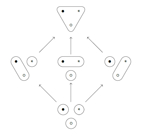 104 |
105 | It looks simple. But that's deceptive! For a 4-element set we get this
106 | poset of partitions:
107 |
108 |
104 |
105 | It looks simple. But that's deceptive! For a 4-element set we get this
106 | poset of partitions:
107 |
108 | 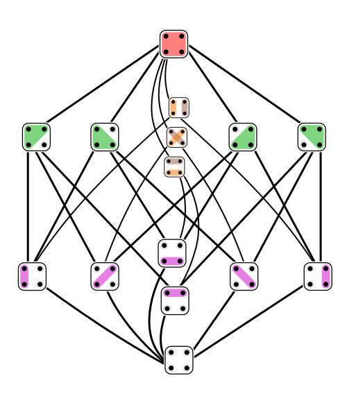 109 |
110 | It's much more complicated than the poset of _subsets_ of a 4-element
111 | set:
112 |
113 |
109 |
110 | It's much more complicated than the poset of _subsets_ of a 4-element
111 | set:
112 |
113 | 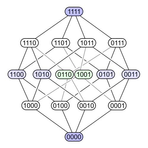 114 |
115 | Indeed, there are many difficult questions about the poset of
116 | partitions that are easy for the poset of subsets.
117 |
118 | For example: how many subsets does an \\(n\\)-element set have? Easy:
119 | \\(2^n\\). But how many partitions does an \\(n\\)-element set have?
120 | Not so easy: it's the \\(n\\)th **[Bell
121 | number](https://en.wikipedia.org/wiki/Bell_number)** \\(B_n\\). The
122 | Bell numbers go like this:
123 |
124 | \\[1, 1, 2, 5, 15, 52, 203, 877, 4140, 21147, 115975, 678570, \dots\\]
125 |
126 | Another example: poset of subsets looks the same when you flip it
127 | upside down. That's because any subset \\(S \subseteq X\\) has a
128 | **complement**
129 |
130 | \\[X - S = \\{x \in X : \; x \notin S \\} .\\]
131 |
132 | In the logic of subsets this gives **negation**: if a subset \\(S
133 | \subseteq X\\) corresponds to some proposition \\(P\\), its complement
134 | \\(X - S\\) corresponds to the proposition \\(\neg P\\), which is how
135 | logicians write "not \\(P\\) ".
136 |
137 | But the poset of partitions does _not_ look the same when you flip it
138 | upside down:
139 |
140 |
141 |
142 | And indeed, there is no "not" in partition logic! It's very different
143 | than classical logic. To read more about it, go here:
144 |
145 | * David Ellerman, [The logic of partitions: introduction to the dual
146 | of the logic of subsets](https://arxiv.org/abs/0902.1950).
147 |
148 | Partition logic still has joins and meets, so I'll talk about those
149 | next time. We should also see how a function \\(f : X \to Y\\) gives a
150 | monotone function \\(f^\ast : \mathcal{E}(Y) \to
151 | \mathcal{E}(X)\\). And we should see if \\(f^\ast\\) has left or right
152 | adjoints!
153 |
154 | This leads up to the punchline of Chapter 1: the idea of "generative
155 | effects". In a nutshell, partition logic has "generative effects"
156 | because the right adjoint of \\(f^*\\) doesn't preserve joins. This
157 | may sound scary and technical, but as we'll see, it captures a basic
158 | fact about reality.
159 |
160 | **[To read other lectures go here.](http://www.azimuthproject.org/azimuth/show/Applied+Category+Theory#Course)**
161 |
162 | ---
163 |
164 | [Click here to read the original discussion.](https://forum.azimuthproject.org/discussion/1991/lecture-11-chapter-1-the-poset-of-partitions/p1)
165 |
166 | ---
167 |
168 | {% include "../LICENSE.md" %}
169 |
--------------------------------------------------------------------------------
/chapter_1/lecture_2.md:
--------------------------------------------------------------------------------
1 | # Lecture 2 - What is Applied Category Theory?
2 | --------
3 |
4 | "Applied category theory" is fairly new, and I should warn you right
5 | away that it's just getting started. While I can point you to some
6 | great applications of category theory outside mathematics and computer
7 | science, if you ask "have categories been successfully applied to X?"
8 | there's a high chance the answer will be no, even if such an
9 | application is possible! It takes time.
10 |
11 | Category theory was created in 1947. _It was created to be
12 | applied_. Mathematicians were having problems connecting topology to
13 | algebra, and Eilenberg and Mac Lane realized that 3 new concepts were
14 | required to solve these problems: category, functor, and natural
15 | transformation. They succeeded wonderfully, and category theory
16 | started growing rapidly: it is now indispensable in the subject of
17 | "algebraic topology", which solves topology problems using algebra.
18 | Later Grothendieck applied category theory to "algebraic geometry",
19 | and used it to prove the Weil Conjectures, some amazing conjectures
20 | relating number theory to geometry. In the process he invented many
21 | other fundamental concepts, like topoi, or toposes. By now category
22 | theory is a very large subject that takes a long time to thoroughly
23 | learn.
24 |
25 | However, these are applications within pure mathematics, and the new
26 | buzzword "applied category theory" refers to applications _outside_
27 | pure mathematics.
28 |
29 | It also mainly means applications outside computer science.
30 |
31 | Category theory has been applied to computer science for a long time
32 | now, at least since the 1960s. That's why a lot of you - maybe even
33 | most of you - are hackers, programmers, software designers, or
34 | computer scientists. You've heard that category theory is good for
35 | you. You probably heard that _before_ the new buzzword "applied
36 | category theory".
37 |
38 | I'm _not_ a programmer. I apologize for this flaw. I know a fair
39 | amount about categories in computer science - but I learned it from
40 | the category theory side, not from hands-on experience in programming.
41 | For example, I understood monads before I heard of Haskell, and my
42 | first reaction was "What are these guys doing with monads? How are
43 | they managing to make such a simple concept so mysterious?" I
44 | understood cartesian closed categories before I understood the lambda
45 | calculus, and I can't imagine myself understanding the lambda calculus
46 | _without_ category theory (though plenty of people do).
47 |
48 | So, this is not a course on "categories in computer science".
49 | Nonetheless, because category theory is about understanding and
50 | organizing abstract data structures, everything I say will be relevant
51 | in some way to computing! Furthermore, several chapters in _Seven
52 | Sketches_ explicitly discuss databases, and type systems, and other
53 | aspects of computer science.
54 |
55 | In the 1990s people started applying category theory to quantum
56 | physics, and quantum gravity. That's how I got interested in category
57 | theory! There are a lot of success stories here by now. And if people
58 | succeed in building [topological quantum
59 | computers](https://en.wikipedia.org/wiki/Topological_quantum_computer),
60 | we'll see technology that can _only be understood using category
61 | theory_.
62 |
63 | More recently, some of us decided that if categories are good for
64 | computer science and physics, maybe we should apply them elsewhere:
65 | engineering, chemistry, biology and beyond. That's what I'm doing
66 | now. I'm applying categories in the DARPA-funded project on [complex
67 | adaptive system
68 | design](https://johncarlosbaez.wordpress.com/2018/02/19/complex-adaptive-systems-part-7/),
69 | I'm being paid by the Silicon Valley startup
70 | [Pyrofex](https://johncarlosbaez.wordpress.com/2018/02/04/pyrofex/) to
71 | do research in category theory, and I've got 8 grad students and a
72 | postdoc studying [networks](http://math.ucr.edu/home/baez/networks/)
73 | using category theory. And it's not just us - it's catching on.
74 |
75 | It's this incipient spread of category theory into many areas of
76 | science and engineering that people mean when they say "applied
77 | category theory".
78 |
79 | I held a workshop on it last year. You can see slides and videos here:
80 |
81 | * [Applied Category Theory](http://math.ucr.edu/home/baez/ACT2017/),
82 | AMS Western Sectional Meeting, U. C. Riverside, 4-5 November 2017.
83 |
84 | This month [Spencer
85 | Breiner](https://www.nist.gov/people/spencer-breiner) and [Eswaran
86 | Subrahmanian](https://www.cmu.edu/epp/people/faculty/eswaran-subrahmanian.html)
87 | ran a workshop pulling together academics and lots of honchos from
88 | industry and government:
89 |
90 | * [Applied Category Theory: Bridging Theory &
91 | Practice](https://johncarlosbaez.wordpress.com/2018/02/17/applied-category-theory-at-nist/),
92 | 15-16 March 2018, National Institute of Standards and Technology,
93 | Gaithersburg, Maryland, USA.
94 |
95 | They took videos and collected talk slides, but for now you can only
96 | read my description - click the link.
97 |
98 | At the end of April there will be a much bigger week-long school
99 | followed by a week-long workshop in the Netherlands:
100 |
101 | * Applied Category Theory (ACT 2018).
102 | [School](https://johncarlosbaez.wordpress.com/2017/10/22/applied-category-theory-2018-adjoint-school/)
103 | 23-27 April 2018 and
104 | [workshop](https://johncarlosbaez.wordpress.com/2017/09/12/act-2018/)
105 | 30 April-4 May 2018 at the [Lorentz
106 | Center](https://www.lorentzcenter.nl/) in Leiden, the Netherlands.
107 | Organized by [Bob Coecke](http://www.cs.ox.ac.uk/bob.coecke/)
108 | (Oxford), [Brendan Fong](http://www.brendanfong.com/) (MIT), [Aleks
109 | Kissinger](http://www.cs.ru.nl/A.Kissinger/) (Nijmegen), [Martha
110 | Lewis](https://www.cs.ox.ac.uk/people/martha.lewis/) (Amsterdam),
111 | and [Joshua Tan](http://joshuatan.com/research) (Oxford).
112 |
113 | There should be a lot to see on YouTube! I'll be there, and I'll keep
114 | you informed.
115 |
116 | These are _all_ the events I know that have "applied category theory"
117 | in the title. The applications have been building up over decades, but
118 | only now have they reached a critical mass, to make it a subject with
119 | its own name.
120 |
121 | The book by Fong and Spivak is a great introduction to category theory
122 | as viewed from this new perspective. So that's what we'll talk about
123 | here!
124 |
125 | **[To read other lectures go here.](http://www.azimuthproject.org/azimuth/show/Applied+Category+Theory#Course)**
126 |
127 | ---
128 |
129 | [Click here to read the original
130 | discussion](https://forum.azimuthproject.org/discussion/1808/lecture-2-what-is-applied-category-theory/p1)
131 |
132 | ---
133 |
134 | {% include "../LICENSE.md" %}
135 |
--------------------------------------------------------------------------------
/chapter_1/lecture_8.md:
--------------------------------------------------------------------------------
1 | # Lecture 8 - The Logic of Subsets
2 | ---
3 |
4 | I'd like to tell you about two kinds of logic. In both, we start with
5 | a set \\(X\\) of "states of the world" and build a set of statements
6 | about the world, also known as "propositions". In the first,
7 | propositions correspond to subsets of \\(X\\). In the second,
8 | propositions correspond to partitions of \\(X\\). In both approaches
9 | we get a _poset_ of propositions where the partial order is
10 | "implication", written \\(\implies\\).
11 |
12 | The first kind of logic is very familiar. We could call it "subset
13 | logic", but it's part of what people usually call "[classical
14 | logic](https://en.wikipedia.org/wiki/Classical_logic)". This is the
15 | sort of logic we learn in school, assuming we learn any at all. The
16 | second kind of logic is less well known: it's called "[partition
17 | logic](https://arxiv.org/abs/0902.1950)". Interestingly, Fong and
18 | Spivak spend more time on the second kind.
19 |
20 | I'll start by talking about the first kind.
21 |
22 | Most of us learn the relation between propositions and subsets, at
23 | least implicitly, when we meet [Venn
24 | diagrams](https://en.wikipedia.org/wiki/Venn_diagram):
25 |
26 |
114 |
115 | Indeed, there are many difficult questions about the poset of
116 | partitions that are easy for the poset of subsets.
117 |
118 | For example: how many subsets does an \\(n\\)-element set have? Easy:
119 | \\(2^n\\). But how many partitions does an \\(n\\)-element set have?
120 | Not so easy: it's the \\(n\\)th **[Bell
121 | number](https://en.wikipedia.org/wiki/Bell_number)** \\(B_n\\). The
122 | Bell numbers go like this:
123 |
124 | \\[1, 1, 2, 5, 15, 52, 203, 877, 4140, 21147, 115975, 678570, \dots\\]
125 |
126 | Another example: poset of subsets looks the same when you flip it
127 | upside down. That's because any subset \\(S \subseteq X\\) has a
128 | **complement**
129 |
130 | \\[X - S = \\{x \in X : \; x \notin S \\} .\\]
131 |
132 | In the logic of subsets this gives **negation**: if a subset \\(S
133 | \subseteq X\\) corresponds to some proposition \\(P\\), its complement
134 | \\(X - S\\) corresponds to the proposition \\(\neg P\\), which is how
135 | logicians write "not \\(P\\) ".
136 |
137 | But the poset of partitions does _not_ look the same when you flip it
138 | upside down:
139 |
140 |
141 |
142 | And indeed, there is no "not" in partition logic! It's very different
143 | than classical logic. To read more about it, go here:
144 |
145 | * David Ellerman, [The logic of partitions: introduction to the dual
146 | of the logic of subsets](https://arxiv.org/abs/0902.1950).
147 |
148 | Partition logic still has joins and meets, so I'll talk about those
149 | next time. We should also see how a function \\(f : X \to Y\\) gives a
150 | monotone function \\(f^\ast : \mathcal{E}(Y) \to
151 | \mathcal{E}(X)\\). And we should see if \\(f^\ast\\) has left or right
152 | adjoints!
153 |
154 | This leads up to the punchline of Chapter 1: the idea of "generative
155 | effects". In a nutshell, partition logic has "generative effects"
156 | because the right adjoint of \\(f^*\\) doesn't preserve joins. This
157 | may sound scary and technical, but as we'll see, it captures a basic
158 | fact about reality.
159 |
160 | **[To read other lectures go here.](http://www.azimuthproject.org/azimuth/show/Applied+Category+Theory#Course)**
161 |
162 | ---
163 |
164 | [Click here to read the original discussion.](https://forum.azimuthproject.org/discussion/1991/lecture-11-chapter-1-the-poset-of-partitions/p1)
165 |
166 | ---
167 |
168 | {% include "../LICENSE.md" %}
169 |
--------------------------------------------------------------------------------
/chapter_1/lecture_2.md:
--------------------------------------------------------------------------------
1 | # Lecture 2 - What is Applied Category Theory?
2 | --------
3 |
4 | "Applied category theory" is fairly new, and I should warn you right
5 | away that it's just getting started. While I can point you to some
6 | great applications of category theory outside mathematics and computer
7 | science, if you ask "have categories been successfully applied to X?"
8 | there's a high chance the answer will be no, even if such an
9 | application is possible! It takes time.
10 |
11 | Category theory was created in 1947. _It was created to be
12 | applied_. Mathematicians were having problems connecting topology to
13 | algebra, and Eilenberg and Mac Lane realized that 3 new concepts were
14 | required to solve these problems: category, functor, and natural
15 | transformation. They succeeded wonderfully, and category theory
16 | started growing rapidly: it is now indispensable in the subject of
17 | "algebraic topology", which solves topology problems using algebra.
18 | Later Grothendieck applied category theory to "algebraic geometry",
19 | and used it to prove the Weil Conjectures, some amazing conjectures
20 | relating number theory to geometry. In the process he invented many
21 | other fundamental concepts, like topoi, or toposes. By now category
22 | theory is a very large subject that takes a long time to thoroughly
23 | learn.
24 |
25 | However, these are applications within pure mathematics, and the new
26 | buzzword "applied category theory" refers to applications _outside_
27 | pure mathematics.
28 |
29 | It also mainly means applications outside computer science.
30 |
31 | Category theory has been applied to computer science for a long time
32 | now, at least since the 1960s. That's why a lot of you - maybe even
33 | most of you - are hackers, programmers, software designers, or
34 | computer scientists. You've heard that category theory is good for
35 | you. You probably heard that _before_ the new buzzword "applied
36 | category theory".
37 |
38 | I'm _not_ a programmer. I apologize for this flaw. I know a fair
39 | amount about categories in computer science - but I learned it from
40 | the category theory side, not from hands-on experience in programming.
41 | For example, I understood monads before I heard of Haskell, and my
42 | first reaction was "What are these guys doing with monads? How are
43 | they managing to make such a simple concept so mysterious?" I
44 | understood cartesian closed categories before I understood the lambda
45 | calculus, and I can't imagine myself understanding the lambda calculus
46 | _without_ category theory (though plenty of people do).
47 |
48 | So, this is not a course on "categories in computer science".
49 | Nonetheless, because category theory is about understanding and
50 | organizing abstract data structures, everything I say will be relevant
51 | in some way to computing! Furthermore, several chapters in _Seven
52 | Sketches_ explicitly discuss databases, and type systems, and other
53 | aspects of computer science.
54 |
55 | In the 1990s people started applying category theory to quantum
56 | physics, and quantum gravity. That's how I got interested in category
57 | theory! There are a lot of success stories here by now. And if people
58 | succeed in building [topological quantum
59 | computers](https://en.wikipedia.org/wiki/Topological_quantum_computer),
60 | we'll see technology that can _only be understood using category
61 | theory_.
62 |
63 | More recently, some of us decided that if categories are good for
64 | computer science and physics, maybe we should apply them elsewhere:
65 | engineering, chemistry, biology and beyond. That's what I'm doing
66 | now. I'm applying categories in the DARPA-funded project on [complex
67 | adaptive system
68 | design](https://johncarlosbaez.wordpress.com/2018/02/19/complex-adaptive-systems-part-7/),
69 | I'm being paid by the Silicon Valley startup
70 | [Pyrofex](https://johncarlosbaez.wordpress.com/2018/02/04/pyrofex/) to
71 | do research in category theory, and I've got 8 grad students and a
72 | postdoc studying [networks](http://math.ucr.edu/home/baez/networks/)
73 | using category theory. And it's not just us - it's catching on.
74 |
75 | It's this incipient spread of category theory into many areas of
76 | science and engineering that people mean when they say "applied
77 | category theory".
78 |
79 | I held a workshop on it last year. You can see slides and videos here:
80 |
81 | * [Applied Category Theory](http://math.ucr.edu/home/baez/ACT2017/),
82 | AMS Western Sectional Meeting, U. C. Riverside, 4-5 November 2017.
83 |
84 | This month [Spencer
85 | Breiner](https://www.nist.gov/people/spencer-breiner) and [Eswaran
86 | Subrahmanian](https://www.cmu.edu/epp/people/faculty/eswaran-subrahmanian.html)
87 | ran a workshop pulling together academics and lots of honchos from
88 | industry and government:
89 |
90 | * [Applied Category Theory: Bridging Theory &
91 | Practice](https://johncarlosbaez.wordpress.com/2018/02/17/applied-category-theory-at-nist/),
92 | 15-16 March 2018, National Institute of Standards and Technology,
93 | Gaithersburg, Maryland, USA.
94 |
95 | They took videos and collected talk slides, but for now you can only
96 | read my description - click the link.
97 |
98 | At the end of April there will be a much bigger week-long school
99 | followed by a week-long workshop in the Netherlands:
100 |
101 | * Applied Category Theory (ACT 2018).
102 | [School](https://johncarlosbaez.wordpress.com/2017/10/22/applied-category-theory-2018-adjoint-school/)
103 | 23-27 April 2018 and
104 | [workshop](https://johncarlosbaez.wordpress.com/2017/09/12/act-2018/)
105 | 30 April-4 May 2018 at the [Lorentz
106 | Center](https://www.lorentzcenter.nl/) in Leiden, the Netherlands.
107 | Organized by [Bob Coecke](http://www.cs.ox.ac.uk/bob.coecke/)
108 | (Oxford), [Brendan Fong](http://www.brendanfong.com/) (MIT), [Aleks
109 | Kissinger](http://www.cs.ru.nl/A.Kissinger/) (Nijmegen), [Martha
110 | Lewis](https://www.cs.ox.ac.uk/people/martha.lewis/) (Amsterdam),
111 | and [Joshua Tan](http://joshuatan.com/research) (Oxford).
112 |
113 | There should be a lot to see on YouTube! I'll be there, and I'll keep
114 | you informed.
115 |
116 | These are _all_ the events I know that have "applied category theory"
117 | in the title. The applications have been building up over decades, but
118 | only now have they reached a critical mass, to make it a subject with
119 | its own name.
120 |
121 | The book by Fong and Spivak is a great introduction to category theory
122 | as viewed from this new perspective. So that's what we'll talk about
123 | here!
124 |
125 | **[To read other lectures go here.](http://www.azimuthproject.org/azimuth/show/Applied+Category+Theory#Course)**
126 |
127 | ---
128 |
129 | [Click here to read the original
130 | discussion](https://forum.azimuthproject.org/discussion/1808/lecture-2-what-is-applied-category-theory/p1)
131 |
132 | ---
133 |
134 | {% include "../LICENSE.md" %}
135 |
--------------------------------------------------------------------------------
/chapter_1/lecture_8.md:
--------------------------------------------------------------------------------
1 | # Lecture 8 - The Logic of Subsets
2 | ---
3 |
4 | I'd like to tell you about two kinds of logic. In both, we start with
5 | a set \\(X\\) of "states of the world" and build a set of statements
6 | about the world, also known as "propositions". In the first,
7 | propositions correspond to subsets of \\(X\\). In the second,
8 | propositions correspond to partitions of \\(X\\). In both approaches
9 | we get a _poset_ of propositions where the partial order is
10 | "implication", written \\(\implies\\).
11 |
12 | The first kind of logic is very familiar. We could call it "subset
13 | logic", but it's part of what people usually call "[classical
14 | logic](https://en.wikipedia.org/wiki/Classical_logic)". This is the
15 | sort of logic we learn in school, assuming we learn any at all. The
16 | second kind of logic is less well known: it's called "[partition
17 | logic](https://arxiv.org/abs/0902.1950)". Interestingly, Fong and
18 | Spivak spend more time on the second kind.
19 |
20 | I'll start by talking about the first kind.
21 |
22 | Most of us learn the relation between propositions and subsets, at
23 | least implicitly, when we meet [Venn
24 | diagrams](https://en.wikipedia.org/wiki/Venn_diagram):
25 |
26 |  28 |
29 | This is a picture of some set \\(X\\) of "states of the world". But
30 | the world here is very tiny: it's just a letter. It can be any letter
31 | in the Latin, Greek or Cyrillic alphabet. Each region in the Venn
32 | diagram is subset of \\(X\\): for example, the upper left circle
33 | contains all the letters in the Greek alphabet. But each region can
34 | also be seen as a proposition: a statement about the world. For
35 | example, the upper left circle corresponds to the proposition "The
36 | letter belongs to the Greek alphabet".
37 |
38 | As a result, everything you can do with subsets of \\(X\\) turns into
39 | something you can do with propositions. Suppose \\(P, Q,\\) and
40 | \\(R\\) are subsets of \\(X\\). We can also think of these as
41 | propositions, and:
42 |
43 | * if \\(P \subseteq Q\\) we say the proposition \\(P\\) **implies**
44 | the proposition \\(Q\\), and we write \\(P \implies Q\\).
45 |
46 | * If \\(P \cap Q = R\\) we say \\(P \textbf { and } Q = R\\).
47 |
48 | * If \\(P \cup Q = R\\) we say the proposition \\(P \textbf{ or } Q =
49 | R\\).
50 |
51 | All the rules obeyed by "subset", "and" and "or" become rules obeyed
52 | by "implies", "and" and "or".
53 |
54 | I hope you know this already, but if you don't, you're in luck: _this
55 | is this most important thing you've heard all year!_ Please think
56 | about it and ask questions until it revolutionizes the way you think
57 | about logic.
58 |
59 | But really, all this stuff is about one particular way of getting a
60 | poset from the set \\(X\\).
61 |
62 | For any set \\(X\\) the **[power
63 | set](https://en.wikipedia.org/wiki/Power_set)** of \\(X\\) is the
64 | collection of all subsets of \\(X\\). We call it \\(P(X)\\). It's a
65 | poset, where the partial ordering is \\(\subseteq\\).
66 |
67 | For example, here is a picture of the poset \\(P(X)\\) when \\(X =
68 | \\{x,y,z\\}\\):
69 |
70 |
28 |
29 | This is a picture of some set \\(X\\) of "states of the world". But
30 | the world here is very tiny: it's just a letter. It can be any letter
31 | in the Latin, Greek or Cyrillic alphabet. Each region in the Venn
32 | diagram is subset of \\(X\\): for example, the upper left circle
33 | contains all the letters in the Greek alphabet. But each region can
34 | also be seen as a proposition: a statement about the world. For
35 | example, the upper left circle corresponds to the proposition "The
36 | letter belongs to the Greek alphabet".
37 |
38 | As a result, everything you can do with subsets of \\(X\\) turns into
39 | something you can do with propositions. Suppose \\(P, Q,\\) and
40 | \\(R\\) are subsets of \\(X\\). We can also think of these as
41 | propositions, and:
42 |
43 | * if \\(P \subseteq Q\\) we say the proposition \\(P\\) **implies**
44 | the proposition \\(Q\\), and we write \\(P \implies Q\\).
45 |
46 | * If \\(P \cap Q = R\\) we say \\(P \textbf { and } Q = R\\).
47 |
48 | * If \\(P \cup Q = R\\) we say the proposition \\(P \textbf{ or } Q =
49 | R\\).
50 |
51 | All the rules obeyed by "subset", "and" and "or" become rules obeyed
52 | by "implies", "and" and "or".
53 |
54 | I hope you know this already, but if you don't, you're in luck: _this
55 | is this most important thing you've heard all year!_ Please think
56 | about it and ask questions until it revolutionizes the way you think
57 | about logic.
58 |
59 | But really, all this stuff is about one particular way of getting a
60 | poset from the set \\(X\\).
61 |
62 | For any set \\(X\\) the **[power
63 | set](https://en.wikipedia.org/wiki/Power_set)** of \\(X\\) is the
64 | collection of all subsets of \\(X\\). We call it \\(P(X)\\). It's a
65 | poset, where the partial ordering is \\(\subseteq\\).
66 |
67 | For example, here is a picture of the poset \\(P(X)\\) when \\(X =
68 | \\{x,y,z\\}\\):
69 |
70 |  72 |
73 | As you can see, it looks like a 3-dimensional cube. Here's a picture
74 | of \\(P(X)\\) when \\(X\\) has 4 elements:
75 |
76 |
72 |
73 | As you can see, it looks like a 3-dimensional cube. Here's a picture
74 | of \\(P(X)\\) when \\(X\\) has 4 elements:
75 |
76 |  78 |
79 | In this picture we say whether each element is in or out of the subset
80 | by writing a 1 or 0. This time we get a 4-dimensional cube.
81 |
82 | What's the union of two subsets \\(S, T \subseteq X\\)? It's the
83 | smallest subset of \\(X\\) that contains both \\(S\\) and \\(T\\) as
84 | subsets. This is an example of a concept we can define in any poset:
85 |
86 | **Definition.** Given a poset \\((A, \le)\\), the **join** of \\(a, b
87 | \in A\\), if it exists, is the least element \\(c \in A\\) such that
88 | \\(a \le c\\) and \\(b \le c\\). We denote the join of \\(a\\) and
89 | \\(b\\) as \\(a \vee b\\).
90 |
91 | Quite generally we can try to think of _any_ poset as a poset of
92 | propositions. Then \\(\vee\\) means "or". In the logic we're studying
93 | today, this poset is \\(P(X)\\) and \\(\vee\\) is just "union", or
94 | \\(\cup\\).
95 |
96 | Similarly, what's the intersection of two subsets \\(S, T \subseteq
97 | X\\)? Well, it's the largest subset of \\(X\\) that is contained as a
98 | subset of both \\(S\\) and \\(T\\). Again this is an example of a
99 | concept we can define in any poset:
100 |
101 | **Definition.** Given a poset \\((A, \le)\\), the **meet** of \\(a, b
102 | \in A\\), if it exists, is the greatest element \\(c \in A\\) such
103 | that \\(c \le a\\) and \\(c \le b\\). We denote the meet of \\(a\\)
104 | and \\(b\\) as \\(a \wedge b\\).
105 |
106 | When we think of a poset as a poset of propositions, \\(\wedge\\)
107 | means "and". When our poset is \\(P(X)\\), \\(\wedge\\) is just
108 | "intersection". \\(\cap\\).
109 |
110 | We could go on with this, and if this were a course on classical logic
111 | I would. But this is a course on applied category theory! So, we
112 | shouldn't just stick with a fixed set \\(X\\). We should see what
113 | happens when we let it vary! We get a poset of propositions for each
114 | set \\(X\\), but all these posets are related to each other.
115 |
116 | I'll talk about this more next time, but let me give you a teaser now.
117 | Say we have two sets \\(X\\) and \\(Y\\) and a function \\(f : X \to
118 | Y\\). Then we get a monotone map from the poset \\(P(Y)\\) to the
119 | poset \\(P(X)\\), called
120 |
121 | \\[f^* : P(Y) \to P(X)\\]
122 |
123 | For any \\(S \in P(Y)\\), the set \\(f^*(S) \in P(X)\\) is defined
124 | like this:
125 |
126 | \\[f^*(S) = \\{ x \in X : \; f(x) \in S \\}\\]
127 |
128 | Next time, I'll show you this monotone map has both a left and a right
129 | adjoint! And these turn out to be connected to the logical concepts of
130 | "there exists" and "for all". I believe this was first discovered by
131 | the great category theorist [Bill
132 | Lawvere](https://www.emis.de/journals/TAC/reprints/articles/16/tr16abs.html).
133 |
134 | So you see, I haven't given up talking about left and right adjoints.
135 | I'm really just getting ready to explain how they show up in logic:
136 | first in good old classical "subset logic", and then in the weird new
137 | "partition logic".
138 |
139 | **[To read other lectures go here.](http://www.azimuthproject.org/azimuth/show/Applied+Category+Theory#Course)**
140 |
141 | ---
142 |
143 | [Click here to read the original discussion.](https://forum.azimuthproject.org/discussion/1921/lecture-8-chapter-1-the-logic-of-subsets/p1)
144 |
145 | ---
146 |
147 | {% include "../LICENSE.md" %}
148 |
--------------------------------------------------------------------------------
/chapter_1/lecture_13.md:
--------------------------------------------------------------------------------
1 | # Lecture 13 - Pulling Back Partitions
2 |
3 | ---
4 |
5 | Last time we studied meets and joins of partitions. We observed an
6 | interesting difference between the two.
7 |
8 | Suppose we have partitions \\(P\\) and \\(Q\\) of a set \\(X\\). To
9 | figure out if two elements \\(x , x' \in X\\) are in the same part of
10 | the meet \\(P \wedge Q\\), it's enough to know if they're the same
11 | part of \\(P\\) and the same part of \\(Q\\), since
12 |
13 | \\[ x \sim_{P \wedge Q} x' \textrm{ if and only if } x \sim_P x'
14 | \textrm{ and } x \sim_Q x'. \\]
15 |
16 | Here \\(x \sim_P x'\\) means that \\(x\\) and \\(x'\\) are in the same
17 | part of \\(P\\), and so on.
18 |
19 | However, this does _not_ work for the join!
20 |
21 | \\[ \textbf{THIS IS FALSE: } \; x \sim_{P \vee Q} x' \textrm{ if and
22 | only if } x \sim_P x' \textrm{ or } x \sim_Q x' . \\]
23 |
24 | To understand this better, the key is to think about the "inclusion"
25 |
26 | \\[ i : \\{x,x'\\} \to X , \\]
27 |
28 | that is, the function sending \\(x\\) and \\(x'\\) to themselves
29 | thought of as elements of \\(X\\). We'll soon see that any partition
30 | \\(P\\) of \\(X\\) can be "pulled back" to a partition
31 | \\(i^{\ast}(P)\\) on the little set \\( \\{x,x'\\} \\). And we'll see
32 | that our observation can be restated as follows:
33 |
34 | \\[ i^{\ast}(P \wedge Q) = i^{\ast}(P) \wedge i^{\ast}(Q) \\]
35 |
36 | but
37 |
38 | \\[ \textbf{THIS IS FALSE: } \; i^{\ast}(P \vee Q) = i^{\ast}(P) \vee
39 | i^{\ast}(Q) . \\]
40 |
41 | This is just a slicker way of saying the exact same thing. But it will
42 | turn out to be more illuminating!
43 |
44 | So how do we "pull back" a partition?
45 |
46 | Suppose we have any function \\(f : X \to Y\\). Given any partition
47 | \\(P\\) of \\(Y\\), we can "pull it back" along \\(f\\) and get a
48 | partition of \\(X\\) which we call \\(f^{\ast}(P)\\). Here's an
49 | example from the book:
50 |
51 |
78 |
79 | In this picture we say whether each element is in or out of the subset
80 | by writing a 1 or 0. This time we get a 4-dimensional cube.
81 |
82 | What's the union of two subsets \\(S, T \subseteq X\\)? It's the
83 | smallest subset of \\(X\\) that contains both \\(S\\) and \\(T\\) as
84 | subsets. This is an example of a concept we can define in any poset:
85 |
86 | **Definition.** Given a poset \\((A, \le)\\), the **join** of \\(a, b
87 | \in A\\), if it exists, is the least element \\(c \in A\\) such that
88 | \\(a \le c\\) and \\(b \le c\\). We denote the join of \\(a\\) and
89 | \\(b\\) as \\(a \vee b\\).
90 |
91 | Quite generally we can try to think of _any_ poset as a poset of
92 | propositions. Then \\(\vee\\) means "or". In the logic we're studying
93 | today, this poset is \\(P(X)\\) and \\(\vee\\) is just "union", or
94 | \\(\cup\\).
95 |
96 | Similarly, what's the intersection of two subsets \\(S, T \subseteq
97 | X\\)? Well, it's the largest subset of \\(X\\) that is contained as a
98 | subset of both \\(S\\) and \\(T\\). Again this is an example of a
99 | concept we can define in any poset:
100 |
101 | **Definition.** Given a poset \\((A, \le)\\), the **meet** of \\(a, b
102 | \in A\\), if it exists, is the greatest element \\(c \in A\\) such
103 | that \\(c \le a\\) and \\(c \le b\\). We denote the meet of \\(a\\)
104 | and \\(b\\) as \\(a \wedge b\\).
105 |
106 | When we think of a poset as a poset of propositions, \\(\wedge\\)
107 | means "and". When our poset is \\(P(X)\\), \\(\wedge\\) is just
108 | "intersection". \\(\cap\\).
109 |
110 | We could go on with this, and if this were a course on classical logic
111 | I would. But this is a course on applied category theory! So, we
112 | shouldn't just stick with a fixed set \\(X\\). We should see what
113 | happens when we let it vary! We get a poset of propositions for each
114 | set \\(X\\), but all these posets are related to each other.
115 |
116 | I'll talk about this more next time, but let me give you a teaser now.
117 | Say we have two sets \\(X\\) and \\(Y\\) and a function \\(f : X \to
118 | Y\\). Then we get a monotone map from the poset \\(P(Y)\\) to the
119 | poset \\(P(X)\\), called
120 |
121 | \\[f^* : P(Y) \to P(X)\\]
122 |
123 | For any \\(S \in P(Y)\\), the set \\(f^*(S) \in P(X)\\) is defined
124 | like this:
125 |
126 | \\[f^*(S) = \\{ x \in X : \; f(x) \in S \\}\\]
127 |
128 | Next time, I'll show you this monotone map has both a left and a right
129 | adjoint! And these turn out to be connected to the logical concepts of
130 | "there exists" and "for all". I believe this was first discovered by
131 | the great category theorist [Bill
132 | Lawvere](https://www.emis.de/journals/TAC/reprints/articles/16/tr16abs.html).
133 |
134 | So you see, I haven't given up talking about left and right adjoints.
135 | I'm really just getting ready to explain how they show up in logic:
136 | first in good old classical "subset logic", and then in the weird new
137 | "partition logic".
138 |
139 | **[To read other lectures go here.](http://www.azimuthproject.org/azimuth/show/Applied+Category+Theory#Course)**
140 |
141 | ---
142 |
143 | [Click here to read the original discussion.](https://forum.azimuthproject.org/discussion/1921/lecture-8-chapter-1-the-logic-of-subsets/p1)
144 |
145 | ---
146 |
147 | {% include "../LICENSE.md" %}
148 |
--------------------------------------------------------------------------------
/chapter_1/lecture_13.md:
--------------------------------------------------------------------------------
1 | # Lecture 13 - Pulling Back Partitions
2 |
3 | ---
4 |
5 | Last time we studied meets and joins of partitions. We observed an
6 | interesting difference between the two.
7 |
8 | Suppose we have partitions \\(P\\) and \\(Q\\) of a set \\(X\\). To
9 | figure out if two elements \\(x , x' \in X\\) are in the same part of
10 | the meet \\(P \wedge Q\\), it's enough to know if they're the same
11 | part of \\(P\\) and the same part of \\(Q\\), since
12 |
13 | \\[ x \sim_{P \wedge Q} x' \textrm{ if and only if } x \sim_P x'
14 | \textrm{ and } x \sim_Q x'. \\]
15 |
16 | Here \\(x \sim_P x'\\) means that \\(x\\) and \\(x'\\) are in the same
17 | part of \\(P\\), and so on.
18 |
19 | However, this does _not_ work for the join!
20 |
21 | \\[ \textbf{THIS IS FALSE: } \; x \sim_{P \vee Q} x' \textrm{ if and
22 | only if } x \sim_P x' \textrm{ or } x \sim_Q x' . \\]
23 |
24 | To understand this better, the key is to think about the "inclusion"
25 |
26 | \\[ i : \\{x,x'\\} \to X , \\]
27 |
28 | that is, the function sending \\(x\\) and \\(x'\\) to themselves
29 | thought of as elements of \\(X\\). We'll soon see that any partition
30 | \\(P\\) of \\(X\\) can be "pulled back" to a partition
31 | \\(i^{\ast}(P)\\) on the little set \\( \\{x,x'\\} \\). And we'll see
32 | that our observation can be restated as follows:
33 |
34 | \\[ i^{\ast}(P \wedge Q) = i^{\ast}(P) \wedge i^{\ast}(Q) \\]
35 |
36 | but
37 |
38 | \\[ \textbf{THIS IS FALSE: } \; i^{\ast}(P \vee Q) = i^{\ast}(P) \vee
39 | i^{\ast}(Q) . \\]
40 |
41 | This is just a slicker way of saying the exact same thing. But it will
42 | turn out to be more illuminating!
43 |
44 | So how do we "pull back" a partition?
45 |
46 | Suppose we have any function \\(f : X \to Y\\). Given any partition
47 | \\(P\\) of \\(Y\\), we can "pull it back" along \\(f\\) and get a
48 | partition of \\(X\\) which we call \\(f^{\ast}(P)\\). Here's an
49 | example from the book:
50 |
51 |  53 |
54 | For any part \\(S\\) of \\(P\\) we can form the set of all elements of
55 | \\(X\\) that map to \\(S\\). This set is just the **preimage** of
56 | \\(S\\) under \\(f\\), which we met in [Lecture 9](lecture_9.md). We
57 | called it
58 |
59 | \\[ f^{\ast}(S) = \\{x \in X: \; f(x) \in S \\}. \\]
60 |
61 | As long as this set is nonempty, we include it our partition
62 | \\(f^{\ast}(P)\\).
63 |
64 | So beware: we are now using the symbol \\(f^{\ast}\\) in two ways: for
65 | the preimage of a subset and for the pullback of a partition. But
66 | these two ways fit together quite nicely, so it'll be okay.
67 |
68 | Summarizing:
69 |
70 | **Definition.** Given a function \\(f : X \to Y\\) and a partition
71 | \\(P\\) of \\(Y\\), define the **pullback** of \\(P\\) along \\(f\\)
72 | to be this partition of \\(X\\):
73 |
74 | \\[ f^{\ast}(P) = \\{ f^{\ast}(S) : \; S \in P \text{ and } f^{\ast}(S)
75 | \ne \emptyset \\} . \\]
76 |
77 | **Puzzle 40.** Show that \\( f^{\ast}(P) \\) really is a partition
78 | using the fact that \\(P\\) is. It's fun to prove this using
79 | properties of the preimage map \\( f^{\ast} : P(Y) \to P(X) \\).
80 |
81 | It's easy to tell if two elements of \\(X\\) are in the same part of
82 | \\(f^{\ast}(P)\\): just map them to \\(Y\\) and see if they land in
83 | the same part of \\(P\\). In other words,
84 |
85 | \\[ x\sim_{f^{\ast}(P)} x' \textrm{ if and only if } f(x) \sim_P f(x')
86 | \\]
87 |
88 | Now for the main point:
89 |
90 | **Proposition.** Given a function \\(f : X \to Y\\) and partitions
91 | \\(P\\) and \\(Q\\) of \\(Y\\), we always have
92 |
93 | \\[ f^{\ast}(P \wedge Q) = f^{\ast}(P) \wedge f^{\ast}(Q) \\]
94 |
95 | but sometimes we have
96 |
97 | \\[ f^{\ast}(P \vee Q) \ne f^{\ast}(P) \vee f^{\ast}(Q) . \\]
98 |
99 | **Proof.** To prove that
100 |
101 | \\[ f^{\ast}(P \wedge Q) = f^{\ast}(P) \wedge f^{\ast}(Q) \\]
102 |
103 | it's enough to prove that they give the same equivalence relation on
104 | \\(X\\). That is, it's enough to show
105 |
106 | $$ x \sim_{f^{\ast}(P \wedge Q)} x' \textrm{ if and only if }
107 | x \sim_{ f^{\ast}(P) \wedge f^{\ast}(Q) } x'. $$
108 |
109 | This looks scary but we just follow our nose. First we rewrite the
110 | right-hand side using our observation about the meet of partitions:
111 |
112 | $$ x \sim_{f^{\ast}(P \wedge Q)} x' \textrm{ if and only if }
113 | x \sim_{ f^{\ast}(P)} x' \textrm{ and } x\sim_{f^{\ast}(Q) } x'.
114 | $$
115 |
116 | Then we rewrite everything using what we just saw about the pullback:
117 |
118 | \\[ f(x) \sim_{P \wedge Q} f(x') \textrm{ if and only if } f(x) \sim_P
119 | f(x') \textrm{ and } f(x) \sim_Q f(x'). \\]
120 |
121 | And this is true, by our observation about the meet of partitions!
122 | So, we're really just stating that observation in a new language.
123 |
124 | To prove that sometimes
125 |
126 | \\[ f^{\ast}(P \vee Q) \ne f^{\ast}(P) \vee f^{\ast}(Q) , \\]
127 |
128 | we just need one example. So, take \\(P\\) and \\(Q\\) to be these two
129 | partitions:
130 |
131 |
53 |
54 | For any part \\(S\\) of \\(P\\) we can form the set of all elements of
55 | \\(X\\) that map to \\(S\\). This set is just the **preimage** of
56 | \\(S\\) under \\(f\\), which we met in [Lecture 9](lecture_9.md). We
57 | called it
58 |
59 | \\[ f^{\ast}(S) = \\{x \in X: \; f(x) \in S \\}. \\]
60 |
61 | As long as this set is nonempty, we include it our partition
62 | \\(f^{\ast}(P)\\).
63 |
64 | So beware: we are now using the symbol \\(f^{\ast}\\) in two ways: for
65 | the preimage of a subset and for the pullback of a partition. But
66 | these two ways fit together quite nicely, so it'll be okay.
67 |
68 | Summarizing:
69 |
70 | **Definition.** Given a function \\(f : X \to Y\\) and a partition
71 | \\(P\\) of \\(Y\\), define the **pullback** of \\(P\\) along \\(f\\)
72 | to be this partition of \\(X\\):
73 |
74 | \\[ f^{\ast}(P) = \\{ f^{\ast}(S) : \; S \in P \text{ and } f^{\ast}(S)
75 | \ne \emptyset \\} . \\]
76 |
77 | **Puzzle 40.** Show that \\( f^{\ast}(P) \\) really is a partition
78 | using the fact that \\(P\\) is. It's fun to prove this using
79 | properties of the preimage map \\( f^{\ast} : P(Y) \to P(X) \\).
80 |
81 | It's easy to tell if two elements of \\(X\\) are in the same part of
82 | \\(f^{\ast}(P)\\): just map them to \\(Y\\) and see if they land in
83 | the same part of \\(P\\). In other words,
84 |
85 | \\[ x\sim_{f^{\ast}(P)} x' \textrm{ if and only if } f(x) \sim_P f(x')
86 | \\]
87 |
88 | Now for the main point:
89 |
90 | **Proposition.** Given a function \\(f : X \to Y\\) and partitions
91 | \\(P\\) and \\(Q\\) of \\(Y\\), we always have
92 |
93 | \\[ f^{\ast}(P \wedge Q) = f^{\ast}(P) \wedge f^{\ast}(Q) \\]
94 |
95 | but sometimes we have
96 |
97 | \\[ f^{\ast}(P \vee Q) \ne f^{\ast}(P) \vee f^{\ast}(Q) . \\]
98 |
99 | **Proof.** To prove that
100 |
101 | \\[ f^{\ast}(P \wedge Q) = f^{\ast}(P) \wedge f^{\ast}(Q) \\]
102 |
103 | it's enough to prove that they give the same equivalence relation on
104 | \\(X\\). That is, it's enough to show
105 |
106 | $$ x \sim_{f^{\ast}(P \wedge Q)} x' \textrm{ if and only if }
107 | x \sim_{ f^{\ast}(P) \wedge f^{\ast}(Q) } x'. $$
108 |
109 | This looks scary but we just follow our nose. First we rewrite the
110 | right-hand side using our observation about the meet of partitions:
111 |
112 | $$ x \sim_{f^{\ast}(P \wedge Q)} x' \textrm{ if and only if }
113 | x \sim_{ f^{\ast}(P)} x' \textrm{ and } x\sim_{f^{\ast}(Q) } x'.
114 | $$
115 |
116 | Then we rewrite everything using what we just saw about the pullback:
117 |
118 | \\[ f(x) \sim_{P \wedge Q} f(x') \textrm{ if and only if } f(x) \sim_P
119 | f(x') \textrm{ and } f(x) \sim_Q f(x'). \\]
120 |
121 | And this is true, by our observation about the meet of partitions!
122 | So, we're really just stating that observation in a new language.
123 |
124 | To prove that sometimes
125 |
126 | \\[ f^{\ast}(P \vee Q) \ne f^{\ast}(P) \vee f^{\ast}(Q) , \\]
127 |
128 | we just need one example. So, take \\(P\\) and \\(Q\\) to be these two
129 | partitions:
130 |
131 |  133 |
134 | They are partitions of the set
135 |
136 | \\[ Y = \\{11, 12, 13, 21, 22, 23 \\}. \\]
137 |
138 | Take \\(X = \\{11,22\\} \\) and let \\(i : X \to Y \\) be the
139 | inclusion of \\(X\\) into \\(Y\\), meaning that
140 |
141 | \\[ i(11) = 11, \quad i(22) = 22 . \\]
142 |
143 | Then compute everything! \\(11\\) and \\(22\\) are in different parts
144 | of \\(i^{\ast}(P)\\):
145 |
146 | \\[ i^{\ast}(P) = \\{ \\{11\\}, \\{22\\} \\} . \\]
147 |
148 | They're also in different parts of \\(i^{\ast}(Q)\\):
149 |
150 | \\[ i^{\ast}(Q) = \\{ \\{11\\}, \\{22\\} \\} .\\]
151 |
152 | Thus, we have
153 |
154 | \\[ i^{\ast}(P) \vee i^{\ast}(Q) = \\{ \\{11\\}, \\{22\\} \\} . \\]
155 |
156 | On the other hand, the join \\(P \vee Q \\) has just two parts:
157 |
158 | \\[ P \vee Q = \\{\\{11,12,13,22,23\\},\\{21\\}\\} . \\]
159 |
160 | If you don't see why, figure out the finest partition that's coarser
161 | than \\(P\\) and \\(Q\\) - that's \\(P \vee Q \\). Since \\(11\\) and
162 | \\(22\\) are in the same parts here, the pullback \\(f^{\ast}(P) \vee
163 | f^{\ast}(Q) \\) has just one part:
164 |
165 | \\[ f^{\ast}(P \vee Q) = \\{ \\{11, 22 \\} \\} . \\]
166 |
167 | So, we have
168 |
169 | \\[ f^{\ast}(P \vee Q) \ne f^{\ast}(P) \vee f^{\ast}(Q) \\]
170 |
171 | as desired. \\( \quad \blacksquare \\)
172 |
173 | Now for the real punchline. The example we just saw was the same as
174 | our example of a "generative effect" in [Lecture 12](lecture_12.md).
175 | So, we have a new way of thinking about generative effects: _the
176 | pullback of partitions preserves meets, but it may not preserve
177 | joins!_
178 |
179 | This is an interesting feature of the logic of partitions. Next time
180 | we'll understand it more deeply by pondering left and right adjoints.
181 | But to warm up, you should compare how meets and joins work in the
182 | logic of subsets:
183 |
184 | **Puzzle 41.** Let \\(f : X \to Y \\) and let \\(f^{\ast} : PY \to PX
185 | \\) be the function sending any subset of \\(Y\\) to its preimage in
186 | \\(X\\). Given \\(S,T \in P(Y) \\), is it always true that
187 |
188 | \\[ f^{\ast}(S \wedge T) = f^{\ast}(S) \wedge f^{\ast}(T)? \\]
189 |
190 | Is it always true that
191 |
192 | \\[ f^{\ast}(S \vee T) = f^{\ast}(S) \vee f^{\ast}(T)? \\]
193 |
194 | **[To read other lectures go here.](http://www.azimuthproject.org/azimuth/show/Applied+Category+Theory#Course)**
195 |
196 | ---
197 |
198 | [Click here to read the original discussion.](https://forum.azimuthproject.org/discussion/2008/lecture-13-chapter-1-pulling-back-partitions/p1)
199 |
200 | ---
201 |
202 | {% include "../LICENSE.md" %}
203 |
--------------------------------------------------------------------------------
/chapter_1/lecture_9.md:
--------------------------------------------------------------------------------
1 | # Lecture 9 - Adjoints and the Logic of Subsets
2 |
3 | ---
4 |
5 | We've seen that classical logic is closely connected to the logic of
6 | subsets. For any set \\(X\\) we get a poset \\(P(X)\\), the **power
7 | set** of \\(X\\), whose elements are _subsets_ of \\(X\\), with the
8 | partial order being \\(\subseteq\\). If \\(X\\) is a set of "states"
9 | of the world, elements of \\(P(X)\\) are "propositions" about the
10 | world. Less grandiosely, if \\(X\\) is the set of states of any
11 | system, elements of \\(P(X)\\) are propositions about that system.
12 |
13 | This trick turns logical operations on propositions - like "and" and
14 | "or" - into operations on subsets, like intersection \\(\cap\\) and
15 | union \\(\cup\\). And these operations are then special cases of
16 | things we can do in _other_ posets, too, like join \\(\vee\\) and meet
17 | \\(\wedge\\).
18 |
19 | We could march much further in this direction. I won't, but try it
20 | yourself!
21 |
22 | **Puzzle 22.** What operation on subsets corresponds to the logical
23 | operation "not"? Describe this operation in the language of posets, so
24 | it has a chance of generalizing to other posets. Based on your
25 | description, find some posets that _do_ have a "not" operation and
26 | some that don't.
27 |
28 | I want to march in another direction. Suppose we have a function
29 | \\(f : X \to Y\\) between sets. This could describe an _observation_,
30 | or _measurement_. For example, \\(X\\) could be the set of states of
31 | your room, and \\(Y\\) could be the set of states of a thermometer in
32 | your room: that is, thermometer readings. Then for any state \\(x\\)
33 | of your room there will be a thermometer reading, the temperature of
34 | your room, which we can call \\(f(x)\\).
35 |
36 | This should yield some function between \\(P(X)\\), the set of
37 | propositions about your room, and \\(P(Y)\\), the set of propositions
38 | about your thermometer. It does. But in fact there are _three_ such
39 | functions! And they're related in a beautiful way!
40 |
41 | The most fundamental is this:
42 |
43 | **Definition.** Suppose \\(f : X \to Y\\) is a function between sets.
44 | For any \\(S \subseteq Y\\) define its **[inverse
45 | image](https://en.wikipedia.org/wiki/Image_(mathematics%29#Inverse_image)**
46 | under \\(f\\) to be
47 |
48 | \\[f^{\ast}(S) = \\{x \in X: \; f(x) \in S\\} .\\]
49 |
50 | The pullback is a subset of \\(X\\).
51 |
52 | The inverse image is also called the **preimage**, and it's often
53 | written as \\(f^{-1}(S)\\). That's okay, but I won't do that: I don't
54 | want to fool you into thinking \\(f\\) needs to have an inverse
55 | \\(f^{-1}\\) - it doesn't. Also, I want to match the notation in
56 | Example 1.89 of _Seven Sketches_.
57 |
58 | The inverse image gives a monotone function
59 |
60 | \\[f^{\ast}: P(Y) \to P(X),\\]
61 |
62 | since if \\(S,T \in P(Y)\\) and \\(S \subseteq T\\) then
63 |
64 | \\[f^{\ast}(S) = \\{x \in X: \; f(x) \in S\\} \subseteq \\{x \in X:\; f(x) \in T\\} = f^{\ast}(T) .\\]
65 |
66 | Why is this so fundamental? Simple: in our example, propositions about
67 | the state of your thermometer give propositions about the state of
68 | your room! If the thermometer says it's 35°, then your room is
69 | 35°, at least near your thermometer. Propositions about the
70 | measuring apparatus are useful because they give propositions about
71 | the system it's measuring - that's what measurement is all about!
72 | This explains the "backwards" nature of the function \\(f^{\ast}: P(Y)
73 | \to P(X)\\), going back from \\(P(Y)\\) to \\(P(X)\\).
74 |
75 | Propositions about the system being measured also give propositions
76 | about the measurement apparatus, but this is more tricky. What does
77 | "there's a living cat in my room" tell us about the temperature I read
78 | on my thermometer? This is a bit confusing... but there is an answer
79 | because a function \\(f\\) really does also give a "forwards" function
80 | from \\(P(X)\\) to \\(P(Y)\\). Here it is:
81 |
82 | **Definition.** Suppose \\(f : X \to Y\\) is a function between sets.
83 | For any \\(S \subseteq X\\) define its
84 | **[image](https://en.wikipedia.org/wiki/Image_(mathematics%29#Image_of_a_subset)**
85 | under \\(f\\) to be
86 |
87 | \\[f_{!}(S) = \\{y \in Y: \; y = f(x) \textrm{ for some } x \in S\\} .\\]
88 |
89 | The image is a subset of \\(Y\\).
90 |
91 | The image is often written as \\(f(S)\\), but I'm using the notation
92 | of _Seven Sketches_, which comes from category theory. People
93 | pronounce \\(f_{!}\\) as "\\(f\\) lower shriek".
94 |
95 | The image gives a monotone function
96 |
97 | \\[f_{!}: P(X) \to P(Y)\\]
98 |
99 | since if \\(S,T \in P(X)\\) and \\(S \subseteq T\\) then
100 |
101 | $$f_{!}(S) = \{y \in Y: \; y = f(x) \textrm{ for some } x \in S \}
102 | \subseteq \{y \in Y: \; y = f(x) \textrm{ for some } x \in T \} =
103 | f_{!}(T) .$$
104 |
105 | But here's the cool part:
106 |
107 | **Theorem.** \\(f_{!}: P(X) \to P(Y)\\) is the left adjoint of
108 | \\(f^{\ast}: P(Y) \to P(X)\\).
109 |
110 | **Proof.** We need to show that for any \\(S \subseteq X\\) and \\(T
111 | \subseteq Y\\) we have
112 |
113 | \\[f_{!}(S) \subseteq T \textrm{ if and only if } S \subseteq
114 | f^{\ast}(T) .\\]
115 |
116 | David Tanzer gave a quick proof in [Puzzle
117 | 19](https://forum.azimuthproject.org/discussion/comment/16490/#Comment_16490).
118 | It goes like this: \\(f_{!}(S) \subseteq T\\) is true if and only if
119 | \\(f\\) maps elements of \\(S\\) to elements of \\(T\\), which is true
120 | if and only if \\(S \subseteq \\{x \in X: \; f(x) \in T\\} =
121 | f^{\ast}(T)\\). \\(\quad \blacksquare\\)
122 |
123 | This is great! But there's also _another_ way to go forwards from
124 | \\(P(X)\\) to \\(P(Y)\\), which is a _right_ adjoint of \\(f^{\ast}:
125 | P(Y) \to P(X)\\). This is less widely known, and I don't even know a
126 | simple name for it. Apparently it's less useful.
127 |
128 | **Definition.** Suppose \\(f : X \to Y\\) is a function between sets.
129 | For any \\(S \subseteq X\\) define
130 |
131 | \\[f_{\ast}(S) = \\{y \in Y: x \in S \textrm{ for all } x \textrm{
132 | such that } y = f(x)\\} .\\]
133 |
134 | This is a subset of \\(Y\\).
135 |
136 | **Puzzle 23.** Show that \\(f_{\ast}: P(X) \to P(Y)\\) is the right
137 | adjoint of \\(f^{\ast}: P(Y) \to P(X)\\).
138 |
139 | What's amazing is this. Here's another way of describing our friend
140 | \\(f_{!}\\). For any \\(S \subseteq X\\) we have
141 |
142 | \\[f_{!}(S) = \\{y \in Y: x \in S \textrm{ for some } x \textrm{ such
143 | that } y = f(x)\\} .\\]
144 |
145 | This looks almost exactly like $$f_{\ast}$$. The only difference is
146 | that while the left adjoint $$f_{!}$$ is defined using "for some", the
147 | right adjoint $$f_{\ast}$$ is defined using "for all". In logic "for
148 | some \\(x\\)" is called the **[existential
149 | quantifier](https://en.wikipedia.org/wiki/Existential_quantification)**
150 | \\(\exists x\\), and "for all \\(x\\)" is called the **[universal
151 | quantifier](https://en.wikipedia.org/wiki/Universal_quantification)**
152 | \\(\forall x\\). So we are seeing that _existential and universal
153 | quantifiers arise as left and right adjoints!_
154 |
155 | This was discovered by Bill Lawvere in this revolutionary paper:
156 |
157 | * F. Willam Lawvere, [Adjointness in
158 | foundations](https://www.emis.de/journals/TAC/reprints/articles/16/tr16abs.html),
159 | _Dialectica_ **23** (1969). Reprinted with author commentary in
160 | _Theory and Applications of Categories_ **16** (2006), 1-16.
161 |
162 | By now this observation is part of a big story that "explains" logic
163 | using category theory.
164 |
165 | Two more puzzles! Let \\(X\\) be the set of states of your room, and
166 | \\(Y\\) the set of states of a thermometer in your room: that is,
167 | thermometer readings. Let \\(f : X \to Y\\) map any state of your room
168 | to the thermometer reading.
169 |
170 | **Puzzle 24.** What is \\(f_{!}(\\{\text{there is a living cat in your
171 | room}\\})\\)? How is this an example of the "liberal" or "generous"
172 | nature of left adjoints, meaning that they're a "best approximation
173 | from above"?
174 |
175 | **Puzzle 25.** What is \\(f_{\ast}(\\{\text{there is a living cat in
176 | your room}\\})\\)? How is this an example of the "conservative" or
177 | "cautious" nature of right adjoints, meaning that they're a "best
178 | approximation from below"?
179 |
180 | **[To read other lectures go here.](http://www.azimuthproject.org/azimuth/show/Applied+Category+Theory#Course)**
181 |
182 | ---
183 |
184 | [Click here to read the original discussion.](https://forum.azimuthproject.org/discussion/1931/lecture-9-chapter-1-adjoints-and-the-logic-of-subsets/p1)
185 |
186 | ---
187 |
188 | {% include "../LICENSE.md" %}
189 |
--------------------------------------------------------------------------------
/chapter_1/lecture_1.md:
--------------------------------------------------------------------------------
1 | # Lecture 1 - Introduction
2 | -----------------------
3 |
4 | Welcome to the **[Applied Category Theory
5 | Course](https://forum.azimuthproject.org/discussion/1717/welcome-to-the-applied-category-theory-course)!**
6 | You can register at left using your full real name as username.
7 |
8 | I haven't carefully counted, but so far about 150 of you have
9 | registered, and I see 27 more applicants whom I haven't gotten around
10 | to approving. A bunch of you have written self-introductions; I
11 | haven't gotten around to responding to all these yet either - but it's
12 | obvious we've got a formidable team here. If we work together we can
13 | do amazing things.
14 |
15 | I decided to teach an online course because I was getting bored of the
16 | superficial engagement I'd been getting on my social media posts,
17 | mainly on [Google+](https://plus.google.com/u/0/+johncbaez999), which
18 | started out great but has been going downhill. I like to explain
19 | things, discuss things and learn things by talking to people. I've
20 | been doing this for decades, first on
21 | [sci.physics.research](https://golem.ph.utexas.edu/category/), and
22 | later on the [n-Category
23 | Café](https://golem.ph.utexas.edu/category/), the [Azimuth
24 | blog](https://johncarlosbaez.wordpress.com/)... and the [Azimuth
25 | Forum](https://forum.azimuthproject.org/discussions) here, which began
26 | life as a platform for creating a wiki about environmental issues: the
27 | [Azimuth Wiki](http://www.azimuthproject.org/azimuth/show/HomePage).
28 | All these fora were great fun, but it seems each one gets a bit stale
29 | after a while, so it's time for something new.
30 |
31 | I decided to teach a course on "applied category theory" because
32 | that's what I'm working on, and my former student [Brendan
33 | Fong](http://www.brendanfong.com/) is doing a postdoc with [David
34 | Spivak](http://math.mit.edu/~dspivak/) at MIT, and they taught a
35 | course on this subject and turned it into a very nice book that you
36 | can download for free:
37 |
38 | * Brendan Fong and David Spivak, _[Seven Sketches in Compositionality: An Invitation to Applied Category Theory](http://math.mit.edu/~dspivak/teaching/sp18/7Sketches.pdf)_.
39 |
40 | Our course will be based on this book. I'll give "lectures" on it -
41 | in print, like this one here - from now until at most September 25th,
42 | when I have to start teaching classes at U. C. Riverside again. The
43 | book has 7 chapters, and we've got at most 6 months. I don't have a
44 | set time-table: we'll have to see how things go. We could be done
45 | much sooner, but it may be fun to go slower and get into more detail.
46 |
47 | I will try to write a short lecture every day or so, sometimes more
48 | than one. But sometimes I'll be busy: most notably, from April 23rd
49 | to May 5th, Brendan, David and I will be in the Netherlands at
50 | [Applied Category Theory
51 | 2018](https://johncarlosbaez.wordpress.com/2017/09/12/act-2018/),
52 | along with 60 other people, and things will get very hectic. Expect a
53 | slowdown or complete silence then. With luck you can watch videos.
54 |
55 | We should do all the exercises in the book. I hope some of you
56 | volunteer to copy these exercises over to the Forum, one at a time, so
57 | we can talk about them here. I'll get the game started but I can't do
58 | everything.
59 |
60 | I will also pose Puzzles. In fact I've [already
61 | started](https://forum.azimuthproject.org/discussion/comment/15878/#Comment_15878)!
62 |
63 | So, your job is to read the book, ask questions, try to do the
64 | Exercises and Puzzles, write your answers here - and most importantly,
65 | discuss everything to death! There will be a place to discuss each
66 | Chapter, and a place to discuss each Lecture and these discussions can
67 | go on indefinitely.
68 |
69 | I will take part in these discussions - that's what I love about
70 | online forums. But if all of you ask lots of questions - and I really
71 | hope you do! - I'll be unable to answer them all myself. So, it's
72 | crucial that _if someone asks a question, and you think you know the
73 | answer, help them out_.
74 |
75 | With luck, we'll all learn a lot of stuff, make a lot of new
76 | friends... and some of us will go ahead to revolutionize human
77 | thought, invent amazing new technologies, and save the planet.
78 |
79 | **Getting to Know Each Other**
80 |
81 | If you're new to the Azimuth Forum, please post a comment about your
82 | interests and background in the category
83 | [Chat](https://forum.azimuthproject.org/categories/Chat). A lot of you
84 | have already done this. So, go read some - and reply to at least one!
85 | Pick one that hasn't gotten any replies yet. I want to go through
86 | them all and reply to every one, but it will take me a while. If you
87 | get to know some other people in the course, it'll be a lot more fun.
88 |
89 | I'd like to keep the discussions on Chapters (of the book) and
90 | Lectures (like this) fairly focused. There is always conversation
91 | drift, and some of that is okay, but if you start wanting to talk
92 | about algebraic geometry or sky-diving or something else that's not
93 | really about the course, please take it to
94 | [Chat](https://forum.azimuthproject.org/categories/Chat). That's a
95 | good place for free-wheeling discussions.
96 |
97 | **Discussions**
98 |
99 | You discuss the Chapters by posting a comment on the appropriate
100 | thread, like this:
101 |
102 | * [Chapter 1](https://forum.azimuthproject.org/discussion/1718/chapter-1).
103 |
104 | You can discuss my Lectures by posting a comment on _its_ thread. If
105 | you have questions or comments on the subject of the course that don't
106 | quite fit into any of these places, you can start a new discussion in
107 | the category [Applied Category Theory
108 | Course](https://forum.azimuthproject.org/categories/applied-category-theory-course).
109 | If you have questions about technical aspects of how the Azimuth Forum
110 | works - or why it's not working - start a discussion in the category
111 | [Technical](https://forum.azimuthproject.org/categories/Technical).
112 |
113 | **Writing math**
114 |
115 | You can write equations using
116 | [MathJax](http://docs.mathjax.org/en/latest/start.html), which is a
117 | limited version of LaTeX good for the web. For "displayed" equations,
118 | centered on the page, use double dollar signs: `$$E = \sqrt{m^2 +
119 | p^2}$$` produces this:
120 |
121 | $$E = \sqrt{m^2 + p^2}$$
122 |
123 | For "inline" equations, mixed in with your text, use this other
124 | method: `\\(E = \sqrt{m^2 + p^2}\\)` produces this: \\(E = \sqrt{m^2 +
125 | p^2}\\). If you don't know anything about LaTeX, you can look at the
126 | source code of other people's comments and see how they're doing
127 | stuff.
128 |
129 | **Resources**
130 |
131 | The book _[Seven
132 | Sketches](http://math.mit.edu/~dspivak/teaching/sp18/7Sketches.pdf)_
133 | has a bibliography with some good reference. Wikipedia is actually
134 | very good for [definitions of terms used in category
135 | theory](https://en.wikipedia.org/wiki/Outline_of_category_theory).
136 | For more advanced material, see the
137 | [nLab](https://ncatlab.org/nlab/show/HomePage). Also try these free
138 | books:
139 |
140 | * Tom Leinster, _[Basic Category
141 | Theory](https://arxiv.org/abs/1612.09375)_, Cambridge Studies in
142 | Advanced Mathematics, Vol. 143, Cambridge University Press, 2014.
143 | (An introduction.)
144 |
145 | * Emily Riehl, _[Category Theory in
146 | Context](http://www.math.jhu.edu/~eriehl/context.pdf)_, Dover, New
147 | York, 2016. (More advanced.)
148 |
149 | **Be nice**
150 |
151 | It's an inevitable feature of any discussion forum that some users
152 | become rude, bully others, try to take over conversations, or try to
153 | promote irrelevant ideas. Anyone who becomes annoying in these or
154 | other ways will be banned. I won't allow discussions about these
155 | issues, either. I have been helping run online discussion forums
156 | since around 1989, back when we used modems, and I've learned that
157 | requiring politeness is the only way to keep attention focused on the
158 | actual subject matter. If you don't want to be polite and respectful
159 | of others, please leave now.
160 |
161 | Pro tip: if someone says something idiotic, like "all categories have
162 | colimits", don't say "You're wrong." Say "Actually not all categories
163 | have colimits: consider for example the category of free groups and
164 | homomorphisms between those." It's amazing how much better people
165 | respond when they don't perceive a correction as being _an attack on
166 | their person_. People are incredibly sensitive things.
167 |
168 | ---
169 |
170 | [Click here to read the original
171 | discussion](https://forum.azimuthproject.org/discussion/1807/lecture-1-introduction/p1)
172 |
173 | ---
174 |
175 | {% include "../LICENSE.md" %}
176 |
--------------------------------------------------------------------------------
133 |
134 | They are partitions of the set
135 |
136 | \\[ Y = \\{11, 12, 13, 21, 22, 23 \\}. \\]
137 |
138 | Take \\(X = \\{11,22\\} \\) and let \\(i : X \to Y \\) be the
139 | inclusion of \\(X\\) into \\(Y\\), meaning that
140 |
141 | \\[ i(11) = 11, \quad i(22) = 22 . \\]
142 |
143 | Then compute everything! \\(11\\) and \\(22\\) are in different parts
144 | of \\(i^{\ast}(P)\\):
145 |
146 | \\[ i^{\ast}(P) = \\{ \\{11\\}, \\{22\\} \\} . \\]
147 |
148 | They're also in different parts of \\(i^{\ast}(Q)\\):
149 |
150 | \\[ i^{\ast}(Q) = \\{ \\{11\\}, \\{22\\} \\} .\\]
151 |
152 | Thus, we have
153 |
154 | \\[ i^{\ast}(P) \vee i^{\ast}(Q) = \\{ \\{11\\}, \\{22\\} \\} . \\]
155 |
156 | On the other hand, the join \\(P \vee Q \\) has just two parts:
157 |
158 | \\[ P \vee Q = \\{\\{11,12,13,22,23\\},\\{21\\}\\} . \\]
159 |
160 | If you don't see why, figure out the finest partition that's coarser
161 | than \\(P\\) and \\(Q\\) - that's \\(P \vee Q \\). Since \\(11\\) and
162 | \\(22\\) are in the same parts here, the pullback \\(f^{\ast}(P) \vee
163 | f^{\ast}(Q) \\) has just one part:
164 |
165 | \\[ f^{\ast}(P \vee Q) = \\{ \\{11, 22 \\} \\} . \\]
166 |
167 | So, we have
168 |
169 | \\[ f^{\ast}(P \vee Q) \ne f^{\ast}(P) \vee f^{\ast}(Q) \\]
170 |
171 | as desired. \\( \quad \blacksquare \\)
172 |
173 | Now for the real punchline. The example we just saw was the same as
174 | our example of a "generative effect" in [Lecture 12](lecture_12.md).
175 | So, we have a new way of thinking about generative effects: _the
176 | pullback of partitions preserves meets, but it may not preserve
177 | joins!_
178 |
179 | This is an interesting feature of the logic of partitions. Next time
180 | we'll understand it more deeply by pondering left and right adjoints.
181 | But to warm up, you should compare how meets and joins work in the
182 | logic of subsets:
183 |
184 | **Puzzle 41.** Let \\(f : X \to Y \\) and let \\(f^{\ast} : PY \to PX
185 | \\) be the function sending any subset of \\(Y\\) to its preimage in
186 | \\(X\\). Given \\(S,T \in P(Y) \\), is it always true that
187 |
188 | \\[ f^{\ast}(S \wedge T) = f^{\ast}(S) \wedge f^{\ast}(T)? \\]
189 |
190 | Is it always true that
191 |
192 | \\[ f^{\ast}(S \vee T) = f^{\ast}(S) \vee f^{\ast}(T)? \\]
193 |
194 | **[To read other lectures go here.](http://www.azimuthproject.org/azimuth/show/Applied+Category+Theory#Course)**
195 |
196 | ---
197 |
198 | [Click here to read the original discussion.](https://forum.azimuthproject.org/discussion/2008/lecture-13-chapter-1-pulling-back-partitions/p1)
199 |
200 | ---
201 |
202 | {% include "../LICENSE.md" %}
203 |
--------------------------------------------------------------------------------
/chapter_1/lecture_9.md:
--------------------------------------------------------------------------------
1 | # Lecture 9 - Adjoints and the Logic of Subsets
2 |
3 | ---
4 |
5 | We've seen that classical logic is closely connected to the logic of
6 | subsets. For any set \\(X\\) we get a poset \\(P(X)\\), the **power
7 | set** of \\(X\\), whose elements are _subsets_ of \\(X\\), with the
8 | partial order being \\(\subseteq\\). If \\(X\\) is a set of "states"
9 | of the world, elements of \\(P(X)\\) are "propositions" about the
10 | world. Less grandiosely, if \\(X\\) is the set of states of any
11 | system, elements of \\(P(X)\\) are propositions about that system.
12 |
13 | This trick turns logical operations on propositions - like "and" and
14 | "or" - into operations on subsets, like intersection \\(\cap\\) and
15 | union \\(\cup\\). And these operations are then special cases of
16 | things we can do in _other_ posets, too, like join \\(\vee\\) and meet
17 | \\(\wedge\\).
18 |
19 | We could march much further in this direction. I won't, but try it
20 | yourself!
21 |
22 | **Puzzle 22.** What operation on subsets corresponds to the logical
23 | operation "not"? Describe this operation in the language of posets, so
24 | it has a chance of generalizing to other posets. Based on your
25 | description, find some posets that _do_ have a "not" operation and
26 | some that don't.
27 |
28 | I want to march in another direction. Suppose we have a function
29 | \\(f : X \to Y\\) between sets. This could describe an _observation_,
30 | or _measurement_. For example, \\(X\\) could be the set of states of
31 | your room, and \\(Y\\) could be the set of states of a thermometer in
32 | your room: that is, thermometer readings. Then for any state \\(x\\)
33 | of your room there will be a thermometer reading, the temperature of
34 | your room, which we can call \\(f(x)\\).
35 |
36 | This should yield some function between \\(P(X)\\), the set of
37 | propositions about your room, and \\(P(Y)\\), the set of propositions
38 | about your thermometer. It does. But in fact there are _three_ such
39 | functions! And they're related in a beautiful way!
40 |
41 | The most fundamental is this:
42 |
43 | **Definition.** Suppose \\(f : X \to Y\\) is a function between sets.
44 | For any \\(S \subseteq Y\\) define its **[inverse
45 | image](https://en.wikipedia.org/wiki/Image_(mathematics%29#Inverse_image)**
46 | under \\(f\\) to be
47 |
48 | \\[f^{\ast}(S) = \\{x \in X: \; f(x) \in S\\} .\\]
49 |
50 | The pullback is a subset of \\(X\\).
51 |
52 | The inverse image is also called the **preimage**, and it's often
53 | written as \\(f^{-1}(S)\\). That's okay, but I won't do that: I don't
54 | want to fool you into thinking \\(f\\) needs to have an inverse
55 | \\(f^{-1}\\) - it doesn't. Also, I want to match the notation in
56 | Example 1.89 of _Seven Sketches_.
57 |
58 | The inverse image gives a monotone function
59 |
60 | \\[f^{\ast}: P(Y) \to P(X),\\]
61 |
62 | since if \\(S,T \in P(Y)\\) and \\(S \subseteq T\\) then
63 |
64 | \\[f^{\ast}(S) = \\{x \in X: \; f(x) \in S\\} \subseteq \\{x \in X:\; f(x) \in T\\} = f^{\ast}(T) .\\]
65 |
66 | Why is this so fundamental? Simple: in our example, propositions about
67 | the state of your thermometer give propositions about the state of
68 | your room! If the thermometer says it's 35°, then your room is
69 | 35°, at least near your thermometer. Propositions about the
70 | measuring apparatus are useful because they give propositions about
71 | the system it's measuring - that's what measurement is all about!
72 | This explains the "backwards" nature of the function \\(f^{\ast}: P(Y)
73 | \to P(X)\\), going back from \\(P(Y)\\) to \\(P(X)\\).
74 |
75 | Propositions about the system being measured also give propositions
76 | about the measurement apparatus, but this is more tricky. What does
77 | "there's a living cat in my room" tell us about the temperature I read
78 | on my thermometer? This is a bit confusing... but there is an answer
79 | because a function \\(f\\) really does also give a "forwards" function
80 | from \\(P(X)\\) to \\(P(Y)\\). Here it is:
81 |
82 | **Definition.** Suppose \\(f : X \to Y\\) is a function between sets.
83 | For any \\(S \subseteq X\\) define its
84 | **[image](https://en.wikipedia.org/wiki/Image_(mathematics%29#Image_of_a_subset)**
85 | under \\(f\\) to be
86 |
87 | \\[f_{!}(S) = \\{y \in Y: \; y = f(x) \textrm{ for some } x \in S\\} .\\]
88 |
89 | The image is a subset of \\(Y\\).
90 |
91 | The image is often written as \\(f(S)\\), but I'm using the notation
92 | of _Seven Sketches_, which comes from category theory. People
93 | pronounce \\(f_{!}\\) as "\\(f\\) lower shriek".
94 |
95 | The image gives a monotone function
96 |
97 | \\[f_{!}: P(X) \to P(Y)\\]
98 |
99 | since if \\(S,T \in P(X)\\) and \\(S \subseteq T\\) then
100 |
101 | $$f_{!}(S) = \{y \in Y: \; y = f(x) \textrm{ for some } x \in S \}
102 | \subseteq \{y \in Y: \; y = f(x) \textrm{ for some } x \in T \} =
103 | f_{!}(T) .$$
104 |
105 | But here's the cool part:
106 |
107 | **Theorem.** \\(f_{!}: P(X) \to P(Y)\\) is the left adjoint of
108 | \\(f^{\ast}: P(Y) \to P(X)\\).
109 |
110 | **Proof.** We need to show that for any \\(S \subseteq X\\) and \\(T
111 | \subseteq Y\\) we have
112 |
113 | \\[f_{!}(S) \subseteq T \textrm{ if and only if } S \subseteq
114 | f^{\ast}(T) .\\]
115 |
116 | David Tanzer gave a quick proof in [Puzzle
117 | 19](https://forum.azimuthproject.org/discussion/comment/16490/#Comment_16490).
118 | It goes like this: \\(f_{!}(S) \subseteq T\\) is true if and only if
119 | \\(f\\) maps elements of \\(S\\) to elements of \\(T\\), which is true
120 | if and only if \\(S \subseteq \\{x \in X: \; f(x) \in T\\} =
121 | f^{\ast}(T)\\). \\(\quad \blacksquare\\)
122 |
123 | This is great! But there's also _another_ way to go forwards from
124 | \\(P(X)\\) to \\(P(Y)\\), which is a _right_ adjoint of \\(f^{\ast}:
125 | P(Y) \to P(X)\\). This is less widely known, and I don't even know a
126 | simple name for it. Apparently it's less useful.
127 |
128 | **Definition.** Suppose \\(f : X \to Y\\) is a function between sets.
129 | For any \\(S \subseteq X\\) define
130 |
131 | \\[f_{\ast}(S) = \\{y \in Y: x \in S \textrm{ for all } x \textrm{
132 | such that } y = f(x)\\} .\\]
133 |
134 | This is a subset of \\(Y\\).
135 |
136 | **Puzzle 23.** Show that \\(f_{\ast}: P(X) \to P(Y)\\) is the right
137 | adjoint of \\(f^{\ast}: P(Y) \to P(X)\\).
138 |
139 | What's amazing is this. Here's another way of describing our friend
140 | \\(f_{!}\\). For any \\(S \subseteq X\\) we have
141 |
142 | \\[f_{!}(S) = \\{y \in Y: x \in S \textrm{ for some } x \textrm{ such
143 | that } y = f(x)\\} .\\]
144 |
145 | This looks almost exactly like $$f_{\ast}$$. The only difference is
146 | that while the left adjoint $$f_{!}$$ is defined using "for some", the
147 | right adjoint $$f_{\ast}$$ is defined using "for all". In logic "for
148 | some \\(x\\)" is called the **[existential
149 | quantifier](https://en.wikipedia.org/wiki/Existential_quantification)**
150 | \\(\exists x\\), and "for all \\(x\\)" is called the **[universal
151 | quantifier](https://en.wikipedia.org/wiki/Universal_quantification)**
152 | \\(\forall x\\). So we are seeing that _existential and universal
153 | quantifiers arise as left and right adjoints!_
154 |
155 | This was discovered by Bill Lawvere in this revolutionary paper:
156 |
157 | * F. Willam Lawvere, [Adjointness in
158 | foundations](https://www.emis.de/journals/TAC/reprints/articles/16/tr16abs.html),
159 | _Dialectica_ **23** (1969). Reprinted with author commentary in
160 | _Theory and Applications of Categories_ **16** (2006), 1-16.
161 |
162 | By now this observation is part of a big story that "explains" logic
163 | using category theory.
164 |
165 | Two more puzzles! Let \\(X\\) be the set of states of your room, and
166 | \\(Y\\) the set of states of a thermometer in your room: that is,
167 | thermometer readings. Let \\(f : X \to Y\\) map any state of your room
168 | to the thermometer reading.
169 |
170 | **Puzzle 24.** What is \\(f_{!}(\\{\text{there is a living cat in your
171 | room}\\})\\)? How is this an example of the "liberal" or "generous"
172 | nature of left adjoints, meaning that they're a "best approximation
173 | from above"?
174 |
175 | **Puzzle 25.** What is \\(f_{\ast}(\\{\text{there is a living cat in
176 | your room}\\})\\)? How is this an example of the "conservative" or
177 | "cautious" nature of right adjoints, meaning that they're a "best
178 | approximation from below"?
179 |
180 | **[To read other lectures go here.](http://www.azimuthproject.org/azimuth/show/Applied+Category+Theory#Course)**
181 |
182 | ---
183 |
184 | [Click here to read the original discussion.](https://forum.azimuthproject.org/discussion/1931/lecture-9-chapter-1-adjoints-and-the-logic-of-subsets/p1)
185 |
186 | ---
187 |
188 | {% include "../LICENSE.md" %}
189 |
--------------------------------------------------------------------------------
/chapter_1/lecture_1.md:
--------------------------------------------------------------------------------
1 | # Lecture 1 - Introduction
2 | -----------------------
3 |
4 | Welcome to the **[Applied Category Theory
5 | Course](https://forum.azimuthproject.org/discussion/1717/welcome-to-the-applied-category-theory-course)!**
6 | You can register at left using your full real name as username.
7 |
8 | I haven't carefully counted, but so far about 150 of you have
9 | registered, and I see 27 more applicants whom I haven't gotten around
10 | to approving. A bunch of you have written self-introductions; I
11 | haven't gotten around to responding to all these yet either - but it's
12 | obvious we've got a formidable team here. If we work together we can
13 | do amazing things.
14 |
15 | I decided to teach an online course because I was getting bored of the
16 | superficial engagement I'd been getting on my social media posts,
17 | mainly on [Google+](https://plus.google.com/u/0/+johncbaez999), which
18 | started out great but has been going downhill. I like to explain
19 | things, discuss things and learn things by talking to people. I've
20 | been doing this for decades, first on
21 | [sci.physics.research](https://golem.ph.utexas.edu/category/), and
22 | later on the [n-Category
23 | Café](https://golem.ph.utexas.edu/category/), the [Azimuth
24 | blog](https://johncarlosbaez.wordpress.com/)... and the [Azimuth
25 | Forum](https://forum.azimuthproject.org/discussions) here, which began
26 | life as a platform for creating a wiki about environmental issues: the
27 | [Azimuth Wiki](http://www.azimuthproject.org/azimuth/show/HomePage).
28 | All these fora were great fun, but it seems each one gets a bit stale
29 | after a while, so it's time for something new.
30 |
31 | I decided to teach a course on "applied category theory" because
32 | that's what I'm working on, and my former student [Brendan
33 | Fong](http://www.brendanfong.com/) is doing a postdoc with [David
34 | Spivak](http://math.mit.edu/~dspivak/) at MIT, and they taught a
35 | course on this subject and turned it into a very nice book that you
36 | can download for free:
37 |
38 | * Brendan Fong and David Spivak, _[Seven Sketches in Compositionality: An Invitation to Applied Category Theory](http://math.mit.edu/~dspivak/teaching/sp18/7Sketches.pdf)_.
39 |
40 | Our course will be based on this book. I'll give "lectures" on it -
41 | in print, like this one here - from now until at most September 25th,
42 | when I have to start teaching classes at U. C. Riverside again. The
43 | book has 7 chapters, and we've got at most 6 months. I don't have a
44 | set time-table: we'll have to see how things go. We could be done
45 | much sooner, but it may be fun to go slower and get into more detail.
46 |
47 | I will try to write a short lecture every day or so, sometimes more
48 | than one. But sometimes I'll be busy: most notably, from April 23rd
49 | to May 5th, Brendan, David and I will be in the Netherlands at
50 | [Applied Category Theory
51 | 2018](https://johncarlosbaez.wordpress.com/2017/09/12/act-2018/),
52 | along with 60 other people, and things will get very hectic. Expect a
53 | slowdown or complete silence then. With luck you can watch videos.
54 |
55 | We should do all the exercises in the book. I hope some of you
56 | volunteer to copy these exercises over to the Forum, one at a time, so
57 | we can talk about them here. I'll get the game started but I can't do
58 | everything.
59 |
60 | I will also pose Puzzles. In fact I've [already
61 | started](https://forum.azimuthproject.org/discussion/comment/15878/#Comment_15878)!
62 |
63 | So, your job is to read the book, ask questions, try to do the
64 | Exercises and Puzzles, write your answers here - and most importantly,
65 | discuss everything to death! There will be a place to discuss each
66 | Chapter, and a place to discuss each Lecture and these discussions can
67 | go on indefinitely.
68 |
69 | I will take part in these discussions - that's what I love about
70 | online forums. But if all of you ask lots of questions - and I really
71 | hope you do! - I'll be unable to answer them all myself. So, it's
72 | crucial that _if someone asks a question, and you think you know the
73 | answer, help them out_.
74 |
75 | With luck, we'll all learn a lot of stuff, make a lot of new
76 | friends... and some of us will go ahead to revolutionize human
77 | thought, invent amazing new technologies, and save the planet.
78 |
79 | **Getting to Know Each Other**
80 |
81 | If you're new to the Azimuth Forum, please post a comment about your
82 | interests and background in the category
83 | [Chat](https://forum.azimuthproject.org/categories/Chat). A lot of you
84 | have already done this. So, go read some - and reply to at least one!
85 | Pick one that hasn't gotten any replies yet. I want to go through
86 | them all and reply to every one, but it will take me a while. If you
87 | get to know some other people in the course, it'll be a lot more fun.
88 |
89 | I'd like to keep the discussions on Chapters (of the book) and
90 | Lectures (like this) fairly focused. There is always conversation
91 | drift, and some of that is okay, but if you start wanting to talk
92 | about algebraic geometry or sky-diving or something else that's not
93 | really about the course, please take it to
94 | [Chat](https://forum.azimuthproject.org/categories/Chat). That's a
95 | good place for free-wheeling discussions.
96 |
97 | **Discussions**
98 |
99 | You discuss the Chapters by posting a comment on the appropriate
100 | thread, like this:
101 |
102 | * [Chapter 1](https://forum.azimuthproject.org/discussion/1718/chapter-1).
103 |
104 | You can discuss my Lectures by posting a comment on _its_ thread. If
105 | you have questions or comments on the subject of the course that don't
106 | quite fit into any of these places, you can start a new discussion in
107 | the category [Applied Category Theory
108 | Course](https://forum.azimuthproject.org/categories/applied-category-theory-course).
109 | If you have questions about technical aspects of how the Azimuth Forum
110 | works - or why it's not working - start a discussion in the category
111 | [Technical](https://forum.azimuthproject.org/categories/Technical).
112 |
113 | **Writing math**
114 |
115 | You can write equations using
116 | [MathJax](http://docs.mathjax.org/en/latest/start.html), which is a
117 | limited version of LaTeX good for the web. For "displayed" equations,
118 | centered on the page, use double dollar signs: `$$E = \sqrt{m^2 +
119 | p^2}$$` produces this:
120 |
121 | $$E = \sqrt{m^2 + p^2}$$
122 |
123 | For "inline" equations, mixed in with your text, use this other
124 | method: `\\(E = \sqrt{m^2 + p^2}\\)` produces this: \\(E = \sqrt{m^2 +
125 | p^2}\\). If you don't know anything about LaTeX, you can look at the
126 | source code of other people's comments and see how they're doing
127 | stuff.
128 |
129 | **Resources**
130 |
131 | The book _[Seven
132 | Sketches](http://math.mit.edu/~dspivak/teaching/sp18/7Sketches.pdf)_
133 | has a bibliography with some good reference. Wikipedia is actually
134 | very good for [definitions of terms used in category
135 | theory](https://en.wikipedia.org/wiki/Outline_of_category_theory).
136 | For more advanced material, see the
137 | [nLab](https://ncatlab.org/nlab/show/HomePage). Also try these free
138 | books:
139 |
140 | * Tom Leinster, _[Basic Category
141 | Theory](https://arxiv.org/abs/1612.09375)_, Cambridge Studies in
142 | Advanced Mathematics, Vol. 143, Cambridge University Press, 2014.
143 | (An introduction.)
144 |
145 | * Emily Riehl, _[Category Theory in
146 | Context](http://www.math.jhu.edu/~eriehl/context.pdf)_, Dover, New
147 | York, 2016. (More advanced.)
148 |
149 | **Be nice**
150 |
151 | It's an inevitable feature of any discussion forum that some users
152 | become rude, bully others, try to take over conversations, or try to
153 | promote irrelevant ideas. Anyone who becomes annoying in these or
154 | other ways will be banned. I won't allow discussions about these
155 | issues, either. I have been helping run online discussion forums
156 | since around 1989, back when we used modems, and I've learned that
157 | requiring politeness is the only way to keep attention focused on the
158 | actual subject matter. If you don't want to be polite and respectful
159 | of others, please leave now.
160 |
161 | Pro tip: if someone says something idiotic, like "all categories have
162 | colimits", don't say "You're wrong." Say "Actually not all categories
163 | have colimits: consider for example the category of free groups and
164 | homomorphisms between those." It's amazing how much better people
165 | respond when they don't perceive a correction as being _an attack on
166 | their person_. People are incredibly sensitive things.
167 |
168 | ---
169 |
170 | [Click here to read the original
171 | discussion](https://forum.azimuthproject.org/discussion/1807/lecture-1-introduction/p1)
172 |
173 | ---
174 |
175 | {% include "../LICENSE.md" %}
176 |
--------------------------------------------------------------------------------