├── reports
└── images
│ ├── roc_all.png
│ ├── roc_curve.png
│ ├── varImprt.png
│ ├── roc_all_zoom.png
│ ├── roc_curve_zoom.png
│ ├── breastCancerWisconsinDataSet_MachineLearning_19_0.png
│ ├── breastCancerWisconsinDataSet_MachineLearning_22_1.png
│ ├── breastCancerWisconsinDataSet_MachineLearning_25_0.png
│ └── breastCancerWisconsinDataSet_MachineLearning_34_0.png
├── models
└── pickle_models
│ ├── model_nn.pkl
│ ├── model_rf.pkl
│ └── model_knn.pkl
├── src
├── r
│ ├── .Rprofile
│ ├── README.md
│ ├── r.Rproj
│ ├── packrat
│ │ ├── packrat.opts
│ │ ├── init.R
│ │ └── packrat.lock
│ ├── random_forest.R
│ ├── breastCancer.R
│ └── breast_cancer.Rmd
├── pyspark
│ ├── breast_cancer_neural_networks.scala
│ ├── breast_cancer_rdd.py
│ ├── breast_cancer_df.py
│ └── breast_cancer_zeppelin_notebook.json
└── python
│ ├── produce_model_metrics.py
│ ├── exploratory_analysis.py
│ ├── data_extraction.py
│ ├── neural_networks.py
│ ├── knn.py
│ ├── random_forest.py
│ ├── model_eval.py
│ └── helper_functions.py
├── notebooks
└── random_forest_files
│ ├── output_36_1.png
│ ├── output_50_0.png
│ ├── output_58_0.png
│ ├── output_65_0.png
│ └── output_67_0.png
├── dash_dashboard
├── dash_breast_cancer.css
├── README.md
├── global_vars.py
└── app.py
├── LICENSE.md
├── requirements.txt
├── .gitignore
└── README.md
/reports/images/roc_all.png:
--------------------------------------------------------------------------------
https://raw.githubusercontent.com/raviolli77/machineLearning_breastCancer_Python/HEAD/reports/images/roc_all.png
--------------------------------------------------------------------------------
/reports/images/roc_curve.png:
--------------------------------------------------------------------------------
https://raw.githubusercontent.com/raviolli77/machineLearning_breastCancer_Python/HEAD/reports/images/roc_curve.png
--------------------------------------------------------------------------------
/reports/images/varImprt.png:
--------------------------------------------------------------------------------
https://raw.githubusercontent.com/raviolli77/machineLearning_breastCancer_Python/HEAD/reports/images/varImprt.png
--------------------------------------------------------------------------------
/models/pickle_models/model_nn.pkl:
--------------------------------------------------------------------------------
https://raw.githubusercontent.com/raviolli77/machineLearning_breastCancer_Python/HEAD/models/pickle_models/model_nn.pkl
--------------------------------------------------------------------------------
/models/pickle_models/model_rf.pkl:
--------------------------------------------------------------------------------
https://raw.githubusercontent.com/raviolli77/machineLearning_breastCancer_Python/HEAD/models/pickle_models/model_rf.pkl
--------------------------------------------------------------------------------
/reports/images/roc_all_zoom.png:
--------------------------------------------------------------------------------
https://raw.githubusercontent.com/raviolli77/machineLearning_breastCancer_Python/HEAD/reports/images/roc_all_zoom.png
--------------------------------------------------------------------------------
/reports/images/roc_curve_zoom.png:
--------------------------------------------------------------------------------
https://raw.githubusercontent.com/raviolli77/machineLearning_breastCancer_Python/HEAD/reports/images/roc_curve_zoom.png
--------------------------------------------------------------------------------
/src/r/.Rprofile:
--------------------------------------------------------------------------------
1 | #### -- Packrat Autoloader (version 0.4.8-1) -- ####
2 | source("packrat/init.R")
3 | #### -- End Packrat Autoloader -- ####
4 |
--------------------------------------------------------------------------------
/models/pickle_models/model_knn.pkl:
--------------------------------------------------------------------------------
https://raw.githubusercontent.com/raviolli77/machineLearning_breastCancer_Python/HEAD/models/pickle_models/model_knn.pkl
--------------------------------------------------------------------------------
/notebooks/random_forest_files/output_36_1.png:
--------------------------------------------------------------------------------
https://raw.githubusercontent.com/raviolli77/machineLearning_breastCancer_Python/HEAD/notebooks/random_forest_files/output_36_1.png
--------------------------------------------------------------------------------
/notebooks/random_forest_files/output_50_0.png:
--------------------------------------------------------------------------------
https://raw.githubusercontent.com/raviolli77/machineLearning_breastCancer_Python/HEAD/notebooks/random_forest_files/output_50_0.png
--------------------------------------------------------------------------------
/notebooks/random_forest_files/output_58_0.png:
--------------------------------------------------------------------------------
https://raw.githubusercontent.com/raviolli77/machineLearning_breastCancer_Python/HEAD/notebooks/random_forest_files/output_58_0.png
--------------------------------------------------------------------------------
/notebooks/random_forest_files/output_65_0.png:
--------------------------------------------------------------------------------
https://raw.githubusercontent.com/raviolli77/machineLearning_breastCancer_Python/HEAD/notebooks/random_forest_files/output_65_0.png
--------------------------------------------------------------------------------
/notebooks/random_forest_files/output_67_0.png:
--------------------------------------------------------------------------------
https://raw.githubusercontent.com/raviolli77/machineLearning_breastCancer_Python/HEAD/notebooks/random_forest_files/output_67_0.png
--------------------------------------------------------------------------------
/src/r/README.md:
--------------------------------------------------------------------------------
1 | # Machine Learning Techniques on Breast Cancer Wisconsin Data Set
2 |
3 | This serves as a sub-directory for the breast cancer project with all r related stuff. More info later
4 |
--------------------------------------------------------------------------------
/reports/images/breastCancerWisconsinDataSet_MachineLearning_19_0.png:
--------------------------------------------------------------------------------
https://raw.githubusercontent.com/raviolli77/machineLearning_breastCancer_Python/HEAD/reports/images/breastCancerWisconsinDataSet_MachineLearning_19_0.png
--------------------------------------------------------------------------------
/reports/images/breastCancerWisconsinDataSet_MachineLearning_22_1.png:
--------------------------------------------------------------------------------
https://raw.githubusercontent.com/raviolli77/machineLearning_breastCancer_Python/HEAD/reports/images/breastCancerWisconsinDataSet_MachineLearning_22_1.png
--------------------------------------------------------------------------------
/reports/images/breastCancerWisconsinDataSet_MachineLearning_25_0.png:
--------------------------------------------------------------------------------
https://raw.githubusercontent.com/raviolli77/machineLearning_breastCancer_Python/HEAD/reports/images/breastCancerWisconsinDataSet_MachineLearning_25_0.png
--------------------------------------------------------------------------------
/reports/images/breastCancerWisconsinDataSet_MachineLearning_34_0.png:
--------------------------------------------------------------------------------
https://raw.githubusercontent.com/raviolli77/machineLearning_breastCancer_Python/HEAD/reports/images/breastCancerWisconsinDataSet_MachineLearning_34_0.png
--------------------------------------------------------------------------------
/src/r/r.Rproj:
--------------------------------------------------------------------------------
1 | Version: 1.0
2 |
3 | RestoreWorkspace: Default
4 | SaveWorkspace: Default
5 | AlwaysSaveHistory: Default
6 |
7 | EnableCodeIndexing: Yes
8 | UseSpacesForTab: Yes
9 | NumSpacesForTab: 2
10 | Encoding: UTF-8
11 |
12 | RnwWeave: Sweave
13 | LaTeX: pdfLaTeX
14 |
--------------------------------------------------------------------------------
/src/r/packrat/packrat.opts:
--------------------------------------------------------------------------------
1 | auto.snapshot: TRUE
2 | use.cache: FALSE
3 | print.banner.on.startup: auto
4 | vcs.ignore.lib: TRUE
5 | vcs.ignore.src: FALSE
6 | external.packages:
7 | local.repos:
8 | load.external.packages.on.startup: TRUE
9 | ignored.packages:
10 | quiet.package.installation: TRUE
11 | snapshot.recommended.packages: FALSE
12 | snapshot.fields:
13 | Imports
14 | Depends
15 | LinkingTo
16 |
--------------------------------------------------------------------------------
/dash_dashboard/dash_breast_cancer.css:
--------------------------------------------------------------------------------
1 | .banner {
2 | height: 75px;
3 | margin: 0px -10px 10px;
4 | background-color: #00878d;
5 | border-radius: 2px;
6 | }
7 |
8 | .banner h2{
9 | color: white;
10 | padding-top: 10px;
11 | margin-left: 2%;
12 | display: inline-block;
13 | }
14 |
15 | table, td, th {
16 | border: 1px solid #ddd;
17 | text-align: left;
18 | }
19 |
20 | table {
21 | border-collapse: collapse;
22 | width: 100%;
23 | }
24 |
25 | th, td {
26 | padding: 15px;
27 | }
28 |
29 |
30 | h1, h2, h3, h4, h5, h6 {
31 | color: #24515d;
32 | font-family: font-family: "Courier New", Courier;
33 | }
34 |
35 | p {
36 | font-family: font-family: "Courier New", Courier;
37 | }
--------------------------------------------------------------------------------
/LICENSE.md:
--------------------------------------------------------------------------------
1 | MIT License
2 |
3 | Copyright (c) 2017 Inertia7
4 |
5 | Permission is hereby granted, free of charge, to any person obtaining a copy of this software and associated documentation files (the "Software"), to deal in the Software without restriction, including without limitation the rights to use, copy, modify, merge, publish, distribute, sublicense, and/or sell copies of the Software, and to permit persons to whom the Software is furnished to do so, subject to the following conditions:
6 |
7 | The above copyright notice and this permission notice shall be included in all copies or substantial portions of the Software.
8 |
9 | THE SOFTWARE IS PROVIDED "AS IS", WITHOUT WARRANTY OF ANY KIND, EXPRESS OR IMPLIED, INCLUDING BUT NOT LIMITED TO THE WARRANTIES OF MERCHANTABILITY, FITNESS FOR A PARTICULAR PURPOSE AND NONINFRINGEMENT. IN NO EVENT SHALL THE AUTHORS OR COPYRIGHT HOLDERS BE LIABLE FOR ANY CLAIM, DAMAGES OR OTHER LIABILITY, WHETHER IN AN ACTION OF CONTRACT, TORT OR OTHERWISE, ARISING FROM, OUT OF OR IN CONNECTION WITH THE SOFTWARE OR THE USE OR OTHER DEALINGS IN THE SOFTWARE.
--------------------------------------------------------------------------------
/dash_dashboard/README.md:
--------------------------------------------------------------------------------
1 | # Dash Dashboard
2 |
3 | This document serves as a `readme` for the subdirectory containing the code for the interactive dashboard made available by [plotly](https://plot.ly/) called [Dash](https://plot.ly/products/dash/).
4 |
5 | To run the application run `app.py` and you're web browser will open the dashboard.
6 |
7 | ## Exploratory Analysis
8 |
9 | This section explores 3 variable interaction with a 3d scatter plot that showcases the relationship between the variables of your choice. Along with showcasing the distribution of the data using histograms seperating the diagnoses.
10 |
11 |  12 |
13 | ## Machine Learning
14 |
15 | This section showcases the machine learning section of the project.
16 | The metrics are as outlined:
17 |
18 | + ROC Curves
19 | + Interactive Confusion Matrix
20 | + Classification Report - outputs the `classification_report` function from `sklearn` in an html table.
21 |
22 |
12 |
13 | ## Machine Learning
14 |
15 | This section showcases the machine learning section of the project.
16 | The metrics are as outlined:
17 |
18 | + ROC Curves
19 | + Interactive Confusion Matrix
20 | + Classification Report - outputs the `classification_report` function from `sklearn` in an html table.
21 |
22 |  23 |
24 | Any questions or suggestions, please let me know!
25 |
--------------------------------------------------------------------------------
/requirements.txt:
--------------------------------------------------------------------------------
1 | appdirs==1.4.3
2 | appnope==0.1.0
3 | bleach==3.1.1
4 | certifi==2018.1.18
5 | chardet==3.0.4
6 | click==6.7
7 | cycler==0.10.0
8 | dash==0.19.0
9 | dash-core-components==0.16.0
10 | dash-html-components==0.8.0
11 | dash-renderer==0.11.1
12 | decorator==4.2.1
13 | entrypoints==0.2.2
14 | Flask==1.0
15 | Flask-Compress==1.4.0
16 | html5lib==0.999999999
17 | idna==2.6
18 | ipykernel==4.6.1
19 | ipython==6.0.0
20 | ipython-genutils==0.2.0
21 | ipywidgets==6.0.0
22 | itsdangerous==0.24
23 | jedi==0.10.2
24 | Jinja2==2.9.6
25 | jsonschema==2.6.0
26 | jupyter==1.0.0
27 | jupyter-client==5.2.3
28 | jupyter-console==5.2.0
29 | jupyter-core==4.4.0
30 | kiwisolver==1.0.1
31 | MarkupSafe==1.0
32 | matplotlib==2.2.2
33 | mistune==0.8.1
34 | nbconvert==5.1.1
35 | nbformat==4.4.0
36 | notebook==5.7.8
37 | numpy==1.14.5
38 | packaging==16.8
39 | pandas==0.23.3
40 | pandocfilters==1.4.1
41 | pexpect==4.2.1
42 | pickleshare==0.7.4
43 | plotly==3.1.0
44 | prometheus-client==0.3.0
45 | prompt-toolkit==1.0.14
46 | ptyprocess==0.5.1
47 | Pygments==2.2.0
48 | pyparsing==2.1.4
49 | python-dateutil==2.6.1
50 | pytz==2017.3
51 | pyzmq==17.1.0
52 | qtconsole==4.3.1
53 | requests==2.20.0
54 | retrying==1.3.3
55 | scikit-learn==0.19.2
56 | scipy==1.1.0
57 | seaborn==0.9.0
58 | Send2Trash==1.5.0
59 | simplegeneric==0.8.1
60 | six==1.11.0
61 | sklearn==0.0
62 | terminado==0.8.1
63 | terminaltables==3.1.0
64 | testpath==0.3
65 | tornado==4.5.1
66 | traitlets==4.3.2
67 | urllib3==1.25.3
68 | virtualenv==15.1.0
69 | wcwidth==0.1.7
70 | webencodings==0.5.1
71 | Werkzeug==0.15.3
72 | widgetsnbextension==2.0.0
73 |
--------------------------------------------------------------------------------
/.gitignore:
--------------------------------------------------------------------------------
1 | .DS_store
2 |
3 | # Rstuff
4 | src/r/packrat/lib*/
5 | src/r/packrat/src/*
6 |
7 | rsconnect/
8 |
9 | # Byte-compiled / optimized / DLL files
10 | __pycache__/
11 | *.py[cod]
12 | *.pyc
13 | *$py.class
14 |
15 | # C extensions
16 | *.so
17 |
18 | # Icebox stuff
19 | ice_box/
20 |
21 | # Distribution / packaging
22 | .Python
23 | build/
24 | develop-eggs/
25 | dist/
26 | downloads/
27 | eggs/
28 | .eggs/
29 | lib/
30 | lib64/
31 | parts/
32 | sdist/
33 | var/
34 | wheels/
35 | *.egg-info/
36 | .installed.cfg
37 | *.egg
38 | MANIFEST
39 |
40 | # PyInstaller
41 | # Usually these files are written by a python script from a template
42 | # before PyInstaller builds the exe, so as to inject date/other infos into it.
43 | *.manifest
44 | *.spec
45 |
46 | # Installer logs
47 | pip-log.txt
48 | pip-delete-this-directory.txt
49 |
50 | # Unit test / coverage reports
51 | htmlcov/
52 | .tox/
53 | .coverage
54 | .coverage.*
55 | .cache
56 | nosetests.xml
57 | coverage.xml
58 | *.cover
59 | .hypothesis/
60 |
61 | # Translations
62 | *.mo
63 | *.pot
64 |
65 | # Django stuff:
66 | *.log
67 | .static_storage/
68 | .media/
69 | local_settings.py
70 |
71 | # Flask stuff:
72 | instance/
73 | .webassets-cache
74 |
75 | # Scrapy stuff:
76 | .scrapy
77 |
78 | # Sphinx documentation
79 | docs/_build/
80 |
81 | # PyBuilder
82 | target/
83 |
84 | # Jupyter Notebook
85 | .ipynb_checkpoints
86 |
87 | # pyenv
88 | .python-version
89 |
90 | # celery beat schedule file
91 | celerybeat-schedule
92 |
93 | # SageMath parsed files
94 | *.sage.py
95 |
96 | # Environments
97 | .env
98 | .venv
99 | env/
100 | venv/
101 | ENV/
102 | env.bak/
103 | venv.bak/
104 |
105 | # Spyder project settings
106 | .spyderproject
107 | .spyproject
108 |
109 | # Rope project settings
110 | .ropeproject
111 |
112 | # mkdocs documentation
113 | /site
114 |
115 | # mypy
116 | .mypy_cache/
117 | # R Stuff
118 | .Rhistory
119 | .Rproj.user
120 |
--------------------------------------------------------------------------------
/src/pyspark/breast_cancer_neural_networks.scala:
--------------------------------------------------------------------------------
1 | // Load appropriate packages
2 | // Neural Networks
3 | // Compatible with Apache Zeppelin
4 | import org.apache.spark.ml.classification.MultilayerPerceptronClassifier
5 | import org.apache.spark.ml.evaluation.MulticlassClassificationEvaluator
6 | import org.apache.spark.ml.feature.MinMaxScaler
7 | import org.apache.spark.mllib.evaluation.BinaryClassificationMetrics
8 | import org.apache.spark.mllib.stat.{MultivariateStatisticalSummary, Statistics}
9 |
10 | // Read in file
11 | val data = spark.read.format("libsvm")
12 | .load("data/data.txt")
13 |
14 | data.collect()
15 |
16 | // Pre-processing
17 | val scaler = new MinMaxScaler()
18 | .setInputCol("features")
19 | .setOutputCol("scaledFeatures")
20 |
21 | val scalerModel = scaler.fit(data)
22 |
23 | val scaledData = scalerModel.transform(data)
24 | println(s"Features scaled to range: [${scaler.getMin}, ${scaler.getMax}]")
25 | scaledData.select("features", "scaledFeatures").show()
26 |
27 | // Changing RDD files variable names to get accurate predictions
28 | val newNames = Seq("label", "oldFeatures", "features")
29 | val data2 = scaledData.toDF(newNames: _*)
30 |
31 | val splits = data2.randomSplit(Array(0.7, 0.3), seed = 1234L)
32 | val trainingSet = splits(0)
33 | val testSet = splits(1)
34 |
35 | trainingSet.select("label", "features").show(25)
36 |
37 | // Neural Networks
38 | val layers = Array[Int](30, 5, 4, 2)
39 |
40 | // Train the Network
41 | val trainer = new MultilayerPerceptronClassifier()
42 | .setLayers(layers)
43 | .setBlockSize(128)
44 | .setSeed(1234L)
45 | .setMaxIter(100)
46 |
47 | val fitNN = trainer.fit(trainingSet)
48 |
49 | // Predict the Test set
50 | val results = fitNN.transform(testSet)
51 | val predictionAndLabelsNN = results.select("prediction", "label")
52 | val evaluator = new MulticlassClassificationEvaluator()
53 | .setMetricName("accuracy")
54 |
55 | println("Test error rate = " + (1 - evaluator.evaluate(predictionAndLabelsNN)))
56 |
57 | println("Test set accuracy = " + evaluator.evaluate(predictionAndLabelsNN))
--------------------------------------------------------------------------------
/src/python/produce_model_metrics.py:
--------------------------------------------------------------------------------
1 | import sys
2 | from sklearn.metrics import roc_curve
3 | from sklearn.metrics import auc
4 |
5 | # Function for All Models to produce Metrics ---------------------
6 |
7 | def produce_model_metrics(fit, test_set, test_class_set, estimator):
8 | """
9 | Purpose
10 | ----------
11 | Function that will return predictions and probability metrics for said
12 | predictions.
13 |
14 | Parameters
15 | ----------
16 | * fit: Fitted model containing the attribute feature_importances_
17 | * test_set: dataframe/array containing the test set values
18 | * test_class_set: array containing the target values for the test set
19 | * estimator: String represenation of appropriate model, can only contain the
20 | following: ['knn', 'rf', 'nn']
21 |
22 | Returns
23 | ----------
24 | Box plot graph for all numeric data in data frame
25 | """
26 | my_estimators = {
27 | 'rf': 'estimators_',
28 | 'nn': 'out_activation_',
29 | 'knn': '_fit_method'
30 | }
31 | try:
32 | # Captures whether first parameter is a model
33 | if not hasattr(fit, 'fit'):
34 | return print("'{0}' is not an instantiated model from scikit-learn".format(fit))
35 |
36 | # Captures whether the model has been trained
37 | if not vars(fit)[my_estimators[estimator]]:
38 | return print("Model does not appear to be trained.")
39 |
40 | except KeyError as e:
41 | raise KeyError("'{0}' does not correspond with the appropriate key inside the estimators dictionary. \
42 | Please refer to function to check `my_estimators` dictionary.".format(estimator))
43 |
44 |
45 | # Outputting predictions and prediction probability
46 | # for test set
47 | predictions = fit.predict(test_set)
48 | accuracy = fit.score(test_set, test_class_set)
49 | # We grab the second array from the output which corresponds to
50 | # to the predicted probabilites of positive classes
51 | # Ordered wrt fit.classes_ in our case [0, 1] where 1 is our positive class
52 | predictions_prob = fit.predict_proba(test_set)[:, 1]
53 | # ROC Curve stuff
54 | fpr, tpr, _ = roc_curve(test_class_set,
55 | predictions_prob,
56 | pos_label = 1)
57 | auc_fit = auc(fpr, tpr)
58 | return {'predictions': predictions,
59 | 'accuracy': accuracy,
60 | 'fpr': fpr,
61 | 'tpr': tpr,
62 | 'auc': auc_fit}
63 |
--------------------------------------------------------------------------------
/src/pyspark/breast_cancer_rdd.py:
--------------------------------------------------------------------------------
1 | # LOAD APPROPRIATE PACKAGE
2 | import numpy as np
3 | from pyspark.context import SparkContext
4 | from pyspark.mllib.util import MLUtils
5 | from pyspark.mllib.tree import DecisionTree, DecisionTreeModel
6 | from pyspark.mllib.tree import RandomForest, RandomForestModel
7 | from pyspark.mllib.evaluation import BinaryClassificationMetrics
8 |
9 | sc = SparkContext.getOrCreate()
10 | data = MLUtils.loadLibSVMFile(sc, 'data/dataLibSVM.txt')
11 | print(data)
12 | # NEXT LET'S CREATE THE APPROPRIATE TRAINING AND TEST SETS
13 | # WE'LL BE SETTING THEM AS 70-30, ALONG WITH SETTING A
14 | # RANDOM SEED GENERATOR TO MAKE MY RESULTS REPRODUCIBLE
15 |
16 | (trainingSet, testSet) = data.randomSplit([0.7, 0.3], seed = 7)
17 |
18 | ##################
19 | # DECISION TREES #
20 | ##################
21 |
22 | fitDT = DecisionTree.trainClassifier(trainingSet,
23 | numClasses=2,
24 | categoricalFeaturesInfo={},
25 | impurity='gini',
26 | maxDepth=3,
27 | maxBins=32)
28 |
29 | print(fitDT.toDebugString())
30 |
31 | predictionsDT = fitDT.predict(testSet.map(lambda x: x.features))
32 |
33 | labelsAndPredictionsDT = testSet.map(lambda lp: lp.label).zip(predictionsDT)
34 |
35 | # Test Error Rate Evaluations
36 |
37 | testErrDT = labelsAndPredictionsDT.filter(lambda (v, p): v != p).count() / float(testSet.count())
38 |
39 | print('Test Error = {0}'.format(testErrDT))
40 |
41 | # Instantiate metrics object
42 | metricsDT = BinaryClassificationMetrics(labelsAndPredictionsDT)
43 |
44 | # Area under ROC curve
45 | print("Area under ROC = {0}".format(metricsDT.areaUnderROC))
46 |
47 | #################
48 | # RANDOM FOREST #
49 | #################
50 |
51 | fitRF = RandomForest.trainClassifier(trainingSet,
52 | numClasses = 2,
53 | categoricalFeaturesInfo = {},
54 | numTrees = 500,
55 | featureSubsetStrategy="auto",
56 | impurity = 'gini', # USING GINI INDEX FOR OUR RANDOM FOREST MODEL
57 | maxDepth = 4,
58 | maxBins = 100)
59 |
60 | predictionsRF = fitRF.predict(testSet.map(lambda x: x.features))
61 |
62 | labelsAndPredictions = testSet.map(lambda lp: lp.label).zip(predictionsRF)
63 |
64 |
65 | testErr = labelsAndPredictions.filter(lambda (v, p): v != p).count() / float(testSet.count())
66 |
67 | print('Test Error = {0}'.format(testErr))
68 | print('Learned classification forest model:')
69 | print(fitRF.toDebugString())
70 |
71 | # Instantiate metrics object
72 | metricsRF = BinaryClassificationMetrics(labelsAndPredictions)
73 |
74 | # Area under ROC curve
75 | print("Area under ROC = {0}".format(metricsRF.areaUnderROC))
76 |
77 | ###################
78 | # NEURAL NETWORKS #
79 | ###################
80 |
81 | # See Scala Script
--------------------------------------------------------------------------------
/src/python/exploratory_analysis.py:
--------------------------------------------------------------------------------
1 | #!/usr/bin/env python3
2 |
3 | #####################################################
4 | ## WISCONSIN BREAST CANCER MACHINE LEARNING ##
5 | #####################################################
6 | #
7 | # Project by Raul Eulogio
8 | #
9 | # Project found at: https://www.inertia7.com/projects/3
10 | # NOTE: Better in jupyter notebook format
11 |
12 | """
13 | Exploratory Analysis
14 | """
15 | import helper_functions as hf
16 | from data_extraction import breast_cancer
17 | import matplotlib.pyplot as plt
18 | import seaborn as sns
19 |
20 | print('''
21 | ########################################
22 | ## DATA FRAME SHAPE AND DTYPES ##
23 | ########################################
24 | ''')
25 |
26 | print("Here's the dimensions of our data frame:\n",
27 | breast_cancer.shape)
28 |
29 | print("Here's the data types of our columns:\n",
30 | breast_cancer.dtypes)
31 |
32 | print("Some more statistics for our data frame: \n",
33 | breast_cancer.describe())
34 |
35 | print('''
36 | ##########################################
37 | ## STATISTICS RELATING TO DX ##
38 | ##########################################
39 | ''')
40 |
41 | # Next let's use the helper function to show distribution
42 | # of our data frame
43 | hf.print_target_perc(breast_cancer, 'diagnosis')
44 | import pdb
45 | pdb.set_trace()
46 | # Scatterplot Matrix
47 | # Variables chosen from Random Forest modeling.
48 |
49 | cols = ['concave_points_worst', 'concavity_mean',
50 | 'perimeter_worst', 'radius_worst',
51 | 'area_worst', 'diagnosis']
52 |
53 | sns.pairplot(breast_cancer,
54 | x_vars = cols,
55 | y_vars = cols,
56 | hue = 'diagnosis',
57 | palette = ('Red', '#875FDB'),
58 | markers=["o", "D"])
59 |
60 | plt.title('Scatterplot Matrix')
61 | plt.show()
62 | plt.close()
63 |
64 | # Pearson Correlation Matrix
65 | corr = breast_cancer.corr(method = 'pearson') # Correlation Matrix
66 | f, ax = plt.subplots(figsize=(11, 9))
67 |
68 | # Generate a custom diverging colormap
69 | cmap = sns.diverging_palette(10, 275, as_cmap=True)
70 |
71 | # Draw the heatmap with the mask and correct aspect ratio
72 | sns.heatmap(corr,
73 | cmap=cmap,
74 | square=True,
75 | xticklabels=True,
76 | yticklabels=True,
77 | linewidths=.5,
78 | cbar_kws={"shrink": .5},
79 | ax=ax)
80 |
81 | plt.title("Pearson Correlation Matrix")
82 | plt.yticks(rotation = 0)
83 | plt.xticks(rotation = 270)
84 | plt.show()
85 | plt.close()
86 |
87 | # BoxPlot
88 | hf.plot_box_plot(breast_cancer, 'Pre-Processed', (-.05, 50))
89 |
90 | # Normalizing data
91 | breast_cancer_norm = hf.normalize_data_frame(breast_cancer)
92 |
93 | # Visuals relating to normalized data to show significant difference
94 | print('''
95 | #################################
96 | ## Transformed Data Statistics ##
97 | #################################
98 | ''')
99 |
100 | print(breast_cancer_norm.describe())
101 |
102 | hf.plot_box_plot(breast_cancer_norm, 'Transformed', (-.05, 1.05))
103 |
--------------------------------------------------------------------------------
/src/python/data_extraction.py:
--------------------------------------------------------------------------------
1 | #!/usr/bin/env python3
2 |
3 | #####################################################
4 | ## WISCONSIN BREAST CANCER MACHINE LEARNING ##
5 | #####################################################
6 | #
7 | # Project by Raul Eulogio
8 | #
9 | # Project found at: https://www.inertia7.com/projects/3
10 | #
11 |
12 | # Import Packages -----------------------------------------------
13 | import numpy as np
14 | import pandas as pd
15 | from sklearn.preprocessing import MinMaxScaler
16 | from sklearn.model_selection import train_test_split
17 | from urllib.request import urlopen
18 |
19 | # Loading data ------------------------------
20 | UCI_data_URL = 'https://archive.ics.uci.edu/ml/machine-learning-databases\
21 | /breast-cancer-wisconsin/wdbc.data'
22 |
23 | names = ['id_number', 'diagnosis', 'radius_mean',
24 | 'texture_mean', 'perimeter_mean', 'area_mean',
25 | 'smoothness_mean', 'compactness_mean',
26 | 'concavity_mean','concave_points_mean',
27 | 'symmetry_mean', 'fractal_dimension_mean',
28 | 'radius_se', 'texture_se', 'perimeter_se',
29 | 'area_se', 'smoothness_se', 'compactness_se',
30 | 'concavity_se', 'concave_points_se',
31 | 'symmetry_se', 'fractal_dimension_se',
32 | 'radius_worst', 'texture_worst',
33 | 'perimeter_worst', 'area_worst',
34 | 'smoothness_worst', 'compactness_worst',
35 | 'concavity_worst', 'concave_points_worst',
36 | 'symmetry_worst', 'fractal_dimension_worst']
37 |
38 | dx = ['Malignant', 'Benign']
39 |
40 | breast_cancer = pd.read_csv(urlopen(UCI_data_URL), names=names)
41 |
42 | # Setting 'id_number' as our index
43 | breast_cancer.set_index(['id_number'], inplace = True)
44 |
45 | # Converted to binary to help later on with models and plots
46 | breast_cancer['diagnosis'] = breast_cancer['diagnosis'].map({'M':1, 'B':0})
47 |
48 | for col in breast_cancer:
49 | pd.to_numeric(col, errors='coerce')
50 |
51 | # For later use in CART models
52 | names_index = names[2:]
53 |
54 | # Create Training and Test Set ----------------------------------
55 | feature_space = breast_cancer.iloc[:,
56 | breast_cancer.columns != 'diagnosis']
57 | feature_class = breast_cancer.iloc[:,
58 | breast_cancer.columns == 'diagnosis']
59 |
60 |
61 | training_set, test_set, class_set, test_class_set = train_test_split(feature_space,
62 | feature_class,
63 | test_size = 0.20,
64 | random_state = 42)
65 |
66 | # Cleaning test sets to avoid future warning messages
67 | class_set = class_set.values.ravel()
68 | test_class_set = test_class_set.values.ravel()
69 |
70 | # Scaling dataframe
71 | scaler = MinMaxScaler()
72 |
73 | scaler.fit(training_set)
74 |
75 | training_set_scaled = scaler.fit_transform(training_set)
76 | test_set_scaled = scaler.transform(test_set)
77 |
--------------------------------------------------------------------------------
/src/python/neural_networks.py:
--------------------------------------------------------------------------------
1 | #!/usr/bin/env python3
2 |
3 | #####################################################
4 | ## WISCONSIN BREAST CANCER MACHINE LEARNING ##
5 | #####################################################
6 | #
7 | # Project by Raul Eulogio
8 | #
9 | # Project found at: https://www.inertia7.com/projects/3
10 | #
11 |
12 | """
13 | Neural Networks Classification
14 | """
15 | # Import Packages -----------------------------------------------
16 | import sys, os
17 | import pandas as pd
18 | import helper_functions as hf
19 | from data_extraction import training_set_scaled, class_set
20 | from data_extraction import test_set_scaled, test_class_set
21 | from sklearn.neural_network import MLPClassifier
22 | from produce_model_metrics import produce_model_metrics
23 |
24 | # Fitting Neural Network ----------------------------------------
25 | # Fit model
26 | fit_nn = MLPClassifier(solver='lbfgs',
27 | hidden_layer_sizes = (12, ),
28 | activation='tanh',
29 | learning_rate_init=0.05,
30 | random_state=42)
31 |
32 | # Train model on training set
33 | fit_nn.fit(training_set_scaled,
34 | class_set)
35 |
36 | if __name__ == '__main__':
37 | # Print model parameters ------------------------------------
38 | print(fit_nn, '\n')
39 |
40 | # Initialize function for metrics ---------------------------
41 | fit_dict_nn = produce_model_metrics(fit_nn, test_set_scaled,
42 | test_class_set, 'nn')
43 | # Extract each piece from dictionary
44 | predictions_nn = fit_dict_nn['predictions']
45 | accuracy_nn = fit_dict_nn['accuracy']
46 | auc_nn = fit_dict_nn['auc']
47 |
48 |
49 | print("Hyperparameter Optimization:")
50 | print("chosen parameters: \n \
51 | {'hidden_layer_sizes': 12, \n \
52 | 'activation': 'tanh', \n \
53 | 'learning_rate_init': 0.05}")
54 | print("Note: Remove commented code to see this section \n")
55 |
56 | # from sklearn.model_selection import GridSearchCV
57 | # import time
58 | # start = time.time()
59 | # gs = GridSearchCV(fit_nn, cv = 10,
60 | # param_grid={
61 | # 'learning_rate_init': [0.05, 0.01, 0.005, 0.001],
62 | # 'hidden_layer_sizes': [4, 8, 12],
63 | # 'activation': ["relu", "identity", "tanh", "logistic"]})
64 | # gs.fit(training_set_scaled, class_set)
65 | # print(gs.best_params_)
66 | # end = time.time()
67 | # print(end - start)
68 |
69 | # Test Set Calculations -------------------------------------
70 | # Test error rate
71 | test_error_rate_nn = 1 - accuracy_nn
72 |
73 | # Confusion Matrix
74 | test_crosstb = hf.create_conf_mat(test_class_set,
75 | predictions_nn)
76 |
77 | # Cross validation
78 | print("Cross Validation:")
79 |
80 | hf.cross_val_metrics(fit_nn,
81 | training_set_scaled,
82 | class_set,
83 | 'nn',
84 | print_results = True)
85 |
86 | print('Confusion Matrix:')
87 | print(test_crosstb, '\n')
88 |
89 | print("Here is our mean accuracy on the test set:\n {0: .3f}"\
90 | .format(accuracy_nn))
91 |
92 | print("The test error rate for our model is:\n {0: .3f}"\
93 | .format(test_error_rate_nn))
94 |
--------------------------------------------------------------------------------
/src/python/knn.py:
--------------------------------------------------------------------------------
1 | #!/usr/bin/env python3
2 |
3 | #####################################################
4 | ## WISCONSIN BREAST CANCER MACHINE LEARNING ##
5 | #####################################################
6 | #
7 | # Project by Raul Eulogio
8 | #
9 | # Project found at: https://www.inertia7.com/projects/3
10 | #
11 |
12 | """
13 | Kth Nearest Neighbor Classification
14 | """
15 | # Import Packages -----------------------------------------------
16 | import sys, os
17 | import pandas as pd
18 | import helper_functions as hf
19 | from data_extraction import training_set, class_set
20 | from data_extraction import test_set, test_class_set
21 | from sklearn.neighbors import KNeighborsClassifier
22 | from sklearn.model_selection import cross_val_score
23 | from produce_model_metrics import produce_model_metrics
24 |
25 | # Fitting model
26 | fit_knn = KNeighborsClassifier(n_neighbors=3)
27 |
28 | # Training model
29 | fit_knn.fit(training_set,
30 | class_set)
31 | # ---------------------------------------------------------------
32 | if __name__ == '__main__':
33 | # Print model parameters ------------------------------------
34 | print(fit_knn, '\n')
35 |
36 | # Optimal K -------------------------------------------------
37 | # Inspired by:
38 | # https://kevinzakka.github.io/2016/07/13/k-nearest-neighbor/
39 |
40 | myKs = []
41 | for i in range(0, 50):
42 | if (i % 2 != 0):
43 | myKs.append(i)
44 |
45 | cross_vals = []
46 | for k in myKs:
47 | knn = KNeighborsClassifier(n_neighbors=k)
48 | scores = cross_val_score(knn,
49 | training_set,
50 | class_set,
51 | cv = 10,
52 | scoring='accuracy')
53 | cross_vals.append(scores.mean())
54 |
55 | MSE = [1 - x for x in cross_vals]
56 | optimal_k = myKs[MSE.index(min(MSE))]
57 | print("Optimal K is {0}".format(optimal_k), '\n')
58 |
59 | # Initialize function for metrics ---------------------------
60 | fit_dict_knn = produce_model_metrics(fit_knn,
61 | test_set,
62 | test_class_set,
63 | 'knn')
64 | # Extract each piece from dictionary
65 | predictions_knn = fit_dict_knn['predictions']
66 | accuracy_knn = fit_dict_knn['accuracy']
67 | auc_knn = fit_dict_knn['auc']
68 |
69 | # Test Set Calculations -------------------------------------
70 | # Test error rate
71 | test_error_rate_knn = 1 - accuracy_knn
72 |
73 | # Confusion Matrix
74 | test_crosstb = hf.create_conf_mat(test_class_set,
75 | predictions_knn)
76 |
77 | print('Cross Validation:')
78 | hf.cross_val_metrics(fit_knn,
79 | training_set,
80 | class_set,
81 | 'knn',
82 | print_results = True)
83 |
84 | print('Confusion Matrix:')
85 | print(test_crosstb, '\n')
86 |
87 | print("Here is our accuracy for our test set:\n {0: .3f}"\
88 | .format(accuracy_knn))
89 |
90 | print("The test error rate for our model is:\n {0: .3f}"\
91 | .format(test_error_rate_knn))
92 |
--------------------------------------------------------------------------------
/dash_dashboard/global_vars.py:
--------------------------------------------------------------------------------
1 | #!/usr/bin/env python3
2 | import sys
3 | import pandas as pd
4 | from sklearn.externals import joblib
5 | from urllib.request import urlopen
6 | from io import StringIO
7 |
8 | # Importing src python scripts ----------------------
9 | sys.path.insert(0, '../src/python/')
10 | from knn import fit_knn
11 | from random_forest import fit_rf
12 | from neural_networks import fit_nn
13 | from data_extraction import test_set_scaled
14 | from data_extraction import test_set, test_class_set
15 | from helper_functions import create_conf_mat
16 | from produce_model_metrics import produce_model_metrics
17 | sys.path.pop(0)
18 |
19 | # Calling up metrics from the model scripts
20 | # KNN -----------------------------------------------
21 | metrics_knn = produce_model_metrics(fit_knn, test_set,
22 | test_class_set, 'knn')
23 | # Call each value from dictionary
24 | predictions_knn = metrics_knn['predictions']
25 | accuracy_knn = metrics_knn['accuracy']
26 | fpr = metrics_knn['fpr']
27 | tpr = metrics_knn['tpr']
28 | auc_knn = metrics_knn['auc']
29 |
30 | test_error_rate_knn = 1 - accuracy_knn
31 |
32 | # Confusion Matrix
33 | cross_tab_knn = create_conf_mat(test_class_set,
34 | predictions_knn)
35 |
36 | # RF ------------------------------------------------
37 | metrics_rf = produce_model_metrics(fit_rf, test_set,
38 | test_class_set, 'rf')
39 | # Call each value from dictionary
40 | predictions_rf = metrics_rf['predictions']
41 | accuracy_rf = metrics_rf['accuracy']
42 | fpr2 = metrics_rf['fpr']
43 | tpr2 = metrics_rf['tpr']
44 | auc_rf = metrics_rf['auc']
45 |
46 | test_error_rate_rf = 1 - accuracy_rf
47 |
48 | cross_tab_rf = create_conf_mat(test_class_set,
49 | predictions_rf)
50 |
51 | # NN ----------------------------------------
52 | metrics_nn = produce_model_metrics(fit_nn, test_set_scaled,
53 | test_class_set, 'nn')
54 |
55 | # Call each value from dictionary
56 | predictions_nn = metrics_nn['predictions']
57 | accuracy_nn = metrics_nn['accuracy']
58 | fpr3 = metrics_nn['fpr']
59 | tpr3 = metrics_nn['tpr']
60 | auc_nn = metrics_nn['auc']
61 |
62 | test_error_rate_nn = 1 - accuracy_nn
63 |
64 | cross_tab_nn = create_conf_mat(test_class_set,
65 | predictions_nn)
66 |
67 | # Classification Report Stuff
68 | def create_class_report(class_report_string):
69 | class_report_mod = StringIO(class_report_string)
70 | class_report = pd.read_csv(class_report_mod, ',')
71 | return class_report
72 |
73 |
74 | class_rep_knn_str = """
75 | Class, Precision, Recall, F1-score, Support
76 | Benign, 0.96, 0.93, 0.94, 73
77 | Malignant, 0.88, 0.93, 0.90, 41
78 | Avg/Total, 0.93, 0.93, 0.93, 114
79 | """
80 |
81 | class_rep_knn = create_class_report(class_rep_knn_str)
82 |
83 | class_rep_rf_str = """
84 | Class, Precision, Recall, F1-score, Support
85 | Benign, 0.99, 0.96, 0.97, 73
86 | Malignant, 0.93, 0.98, 0.95, 41
87 | Avg/Total, 0.97, 0.96, 0.97, 114
88 | """
89 |
90 | class_rep_rf = create_class_report(class_rep_rf_str)
91 |
92 | class_rep_nn_str = """
93 | Class, Precision, Recall, F1-score, Support
94 | Benign , 0.99, 0.97, 0.98, 73
95 | Malignant, 0.95, 0.98, 0.96, 41
96 | Avg/Total, 0.97, 0.97, 0.97, 114
97 | """
98 |
99 | class_rep_nn = create_class_report(class_rep_nn_str)
100 |
--------------------------------------------------------------------------------
/README.md:
--------------------------------------------------------------------------------
1 | # Machine Learning Techniques on Breast Cancer Wisconsin Data Set
2 |
3 | **Contributor**:
4 | + Raul Eulogio
5 |
6 | I created this repo as a way to get better acquainted with **Python** as a language and as a tool for data analysis. But it eventually became in exercise in utilizing various programming languages for machine learning applications.
7 |
8 | I employed four **Machine Learning** techniques:
9 | + **Kth Nearest Neighbor**
10 | + **Random Forest**
11 | + **Neural Networks**:
12 |
13 | If you would like to see a walk through of the analysis on [inertia7](https://www.inertia7.com/projects/3) includes running code as well as explanations for exploratory analysis. This [project](https://www.inertia7.com/projects/95) contains an overview of *random forest*, explanations for other algorithms in the works.
14 |
15 | The repository includes the *scripts* folder which contains scripts for these programming languages (in order of most detailed):
16 | + *Python*
17 | + *R*
18 | + *PySpark*
19 |
20 | This repo is primarily concerned with the *python* iteration.
21 |
22 | The multiple *python* script is broken into 5 sections (done by creating a script for each section) in the following order:
23 | + **Exploratory Analysis**
24 | + **Kth Nearest Neighbors**
25 | + **Random Forest**
26 | + **Neural Networks**
27 | + **Comparing Models**
28 |
29 | **NOTE**: The files `data_extraction.py`, `helper_functions.py`, and `produce_model_metrics.py` are used to abstract functions to make code easier to read. These files do a lot of the work so if you are interested in how the scripts work definitely check them out.
30 |
31 | ## Running .py Script
32 | A `virtualenv` is needed where you will download the necessary packages from the `requirements.txt` using:
33 |
34 | pip3 install -r requirements.txt
35 |
36 | Once this is done you can run the scripts using the usual terminal command:
37 |
38 | $ python3 exploratory_analysis.py
39 |
40 | **NOTE**: You can also run it by making script executable as such:
41 |
42 | $ chmod +x exploratory_analysis.py
43 |
44 |
45 | **Remember**: You must have a *shebang* for this to run i.e. this must be at the very beginning of your script:
46 |
47 | #!/usr/bin/env python3
48 |
49 | then you would simply just run it (I'll use **Random Forest** as an example)
50 |
51 | $ ./random_forest.py
52 |
53 | ## Conclusions
54 | Once I employed all these methods, we were able to utilize various machine learning metrics. Each model provided valuable insight. *Kth Nearest Neighbor* helped create a baseline model to compare the more complex models. *Random forest* helps us see what variables were important in the bootstrapped decision trees. And *Neural Networks* provided minimal false negatives which results in false negatives. In this context it can mean death.
55 |
56 | ### Diagnostics for Data Set
57 |
58 |
59 | | Model/Algorithm | Test Error Rate | False Negative for Test Set | Area under the Curve for ROC | Cross Validation Score | Hyperparameter Optimization |
60 | |----------------------|-----------------|-----------------------------|------------------------------|-------------------------------|-----------------------|
61 | | Kth Nearest Neighbor | 0.07 | 5 | 0.980 | Accuracy: 0.925 (+/- 0.025) | Optimal *K* is 3 |
62 | | Random Forest | 0.035 | 3 | 0.996 | Accuracy: 0.963 (+/- 0.013) | {'max_features': 'log2', 'max_depth': 3, 'bootstrap': True, 'criterion': 'gini'} |
63 | | Neural Networks | 0.035 | 1 | 0.982 | Accuracy: 0.967 (+/- 0.011) | {'hidden_layer_sizes': 12, 'activation': 'tanh', 'learning_rate_init': 0.05} |
64 |
65 |
66 |
67 | #### ROC Curves for Data Set
68 |
23 |
24 | Any questions or suggestions, please let me know!
25 |
--------------------------------------------------------------------------------
/requirements.txt:
--------------------------------------------------------------------------------
1 | appdirs==1.4.3
2 | appnope==0.1.0
3 | bleach==3.1.1
4 | certifi==2018.1.18
5 | chardet==3.0.4
6 | click==6.7
7 | cycler==0.10.0
8 | dash==0.19.0
9 | dash-core-components==0.16.0
10 | dash-html-components==0.8.0
11 | dash-renderer==0.11.1
12 | decorator==4.2.1
13 | entrypoints==0.2.2
14 | Flask==1.0
15 | Flask-Compress==1.4.0
16 | html5lib==0.999999999
17 | idna==2.6
18 | ipykernel==4.6.1
19 | ipython==6.0.0
20 | ipython-genutils==0.2.0
21 | ipywidgets==6.0.0
22 | itsdangerous==0.24
23 | jedi==0.10.2
24 | Jinja2==2.9.6
25 | jsonschema==2.6.0
26 | jupyter==1.0.0
27 | jupyter-client==5.2.3
28 | jupyter-console==5.2.0
29 | jupyter-core==4.4.0
30 | kiwisolver==1.0.1
31 | MarkupSafe==1.0
32 | matplotlib==2.2.2
33 | mistune==0.8.1
34 | nbconvert==5.1.1
35 | nbformat==4.4.0
36 | notebook==5.7.8
37 | numpy==1.14.5
38 | packaging==16.8
39 | pandas==0.23.3
40 | pandocfilters==1.4.1
41 | pexpect==4.2.1
42 | pickleshare==0.7.4
43 | plotly==3.1.0
44 | prometheus-client==0.3.0
45 | prompt-toolkit==1.0.14
46 | ptyprocess==0.5.1
47 | Pygments==2.2.0
48 | pyparsing==2.1.4
49 | python-dateutil==2.6.1
50 | pytz==2017.3
51 | pyzmq==17.1.0
52 | qtconsole==4.3.1
53 | requests==2.20.0
54 | retrying==1.3.3
55 | scikit-learn==0.19.2
56 | scipy==1.1.0
57 | seaborn==0.9.0
58 | Send2Trash==1.5.0
59 | simplegeneric==0.8.1
60 | six==1.11.0
61 | sklearn==0.0
62 | terminado==0.8.1
63 | terminaltables==3.1.0
64 | testpath==0.3
65 | tornado==4.5.1
66 | traitlets==4.3.2
67 | urllib3==1.25.3
68 | virtualenv==15.1.0
69 | wcwidth==0.1.7
70 | webencodings==0.5.1
71 | Werkzeug==0.15.3
72 | widgetsnbextension==2.0.0
73 |
--------------------------------------------------------------------------------
/.gitignore:
--------------------------------------------------------------------------------
1 | .DS_store
2 |
3 | # Rstuff
4 | src/r/packrat/lib*/
5 | src/r/packrat/src/*
6 |
7 | rsconnect/
8 |
9 | # Byte-compiled / optimized / DLL files
10 | __pycache__/
11 | *.py[cod]
12 | *.pyc
13 | *$py.class
14 |
15 | # C extensions
16 | *.so
17 |
18 | # Icebox stuff
19 | ice_box/
20 |
21 | # Distribution / packaging
22 | .Python
23 | build/
24 | develop-eggs/
25 | dist/
26 | downloads/
27 | eggs/
28 | .eggs/
29 | lib/
30 | lib64/
31 | parts/
32 | sdist/
33 | var/
34 | wheels/
35 | *.egg-info/
36 | .installed.cfg
37 | *.egg
38 | MANIFEST
39 |
40 | # PyInstaller
41 | # Usually these files are written by a python script from a template
42 | # before PyInstaller builds the exe, so as to inject date/other infos into it.
43 | *.manifest
44 | *.spec
45 |
46 | # Installer logs
47 | pip-log.txt
48 | pip-delete-this-directory.txt
49 |
50 | # Unit test / coverage reports
51 | htmlcov/
52 | .tox/
53 | .coverage
54 | .coverage.*
55 | .cache
56 | nosetests.xml
57 | coverage.xml
58 | *.cover
59 | .hypothesis/
60 |
61 | # Translations
62 | *.mo
63 | *.pot
64 |
65 | # Django stuff:
66 | *.log
67 | .static_storage/
68 | .media/
69 | local_settings.py
70 |
71 | # Flask stuff:
72 | instance/
73 | .webassets-cache
74 |
75 | # Scrapy stuff:
76 | .scrapy
77 |
78 | # Sphinx documentation
79 | docs/_build/
80 |
81 | # PyBuilder
82 | target/
83 |
84 | # Jupyter Notebook
85 | .ipynb_checkpoints
86 |
87 | # pyenv
88 | .python-version
89 |
90 | # celery beat schedule file
91 | celerybeat-schedule
92 |
93 | # SageMath parsed files
94 | *.sage.py
95 |
96 | # Environments
97 | .env
98 | .venv
99 | env/
100 | venv/
101 | ENV/
102 | env.bak/
103 | venv.bak/
104 |
105 | # Spyder project settings
106 | .spyderproject
107 | .spyproject
108 |
109 | # Rope project settings
110 | .ropeproject
111 |
112 | # mkdocs documentation
113 | /site
114 |
115 | # mypy
116 | .mypy_cache/
117 | # R Stuff
118 | .Rhistory
119 | .Rproj.user
120 |
--------------------------------------------------------------------------------
/src/pyspark/breast_cancer_neural_networks.scala:
--------------------------------------------------------------------------------
1 | // Load appropriate packages
2 | // Neural Networks
3 | // Compatible with Apache Zeppelin
4 | import org.apache.spark.ml.classification.MultilayerPerceptronClassifier
5 | import org.apache.spark.ml.evaluation.MulticlassClassificationEvaluator
6 | import org.apache.spark.ml.feature.MinMaxScaler
7 | import org.apache.spark.mllib.evaluation.BinaryClassificationMetrics
8 | import org.apache.spark.mllib.stat.{MultivariateStatisticalSummary, Statistics}
9 |
10 | // Read in file
11 | val data = spark.read.format("libsvm")
12 | .load("data/data.txt")
13 |
14 | data.collect()
15 |
16 | // Pre-processing
17 | val scaler = new MinMaxScaler()
18 | .setInputCol("features")
19 | .setOutputCol("scaledFeatures")
20 |
21 | val scalerModel = scaler.fit(data)
22 |
23 | val scaledData = scalerModel.transform(data)
24 | println(s"Features scaled to range: [${scaler.getMin}, ${scaler.getMax}]")
25 | scaledData.select("features", "scaledFeatures").show()
26 |
27 | // Changing RDD files variable names to get accurate predictions
28 | val newNames = Seq("label", "oldFeatures", "features")
29 | val data2 = scaledData.toDF(newNames: _*)
30 |
31 | val splits = data2.randomSplit(Array(0.7, 0.3), seed = 1234L)
32 | val trainingSet = splits(0)
33 | val testSet = splits(1)
34 |
35 | trainingSet.select("label", "features").show(25)
36 |
37 | // Neural Networks
38 | val layers = Array[Int](30, 5, 4, 2)
39 |
40 | // Train the Network
41 | val trainer = new MultilayerPerceptronClassifier()
42 | .setLayers(layers)
43 | .setBlockSize(128)
44 | .setSeed(1234L)
45 | .setMaxIter(100)
46 |
47 | val fitNN = trainer.fit(trainingSet)
48 |
49 | // Predict the Test set
50 | val results = fitNN.transform(testSet)
51 | val predictionAndLabelsNN = results.select("prediction", "label")
52 | val evaluator = new MulticlassClassificationEvaluator()
53 | .setMetricName("accuracy")
54 |
55 | println("Test error rate = " + (1 - evaluator.evaluate(predictionAndLabelsNN)))
56 |
57 | println("Test set accuracy = " + evaluator.evaluate(predictionAndLabelsNN))
--------------------------------------------------------------------------------
/src/python/produce_model_metrics.py:
--------------------------------------------------------------------------------
1 | import sys
2 | from sklearn.metrics import roc_curve
3 | from sklearn.metrics import auc
4 |
5 | # Function for All Models to produce Metrics ---------------------
6 |
7 | def produce_model_metrics(fit, test_set, test_class_set, estimator):
8 | """
9 | Purpose
10 | ----------
11 | Function that will return predictions and probability metrics for said
12 | predictions.
13 |
14 | Parameters
15 | ----------
16 | * fit: Fitted model containing the attribute feature_importances_
17 | * test_set: dataframe/array containing the test set values
18 | * test_class_set: array containing the target values for the test set
19 | * estimator: String represenation of appropriate model, can only contain the
20 | following: ['knn', 'rf', 'nn']
21 |
22 | Returns
23 | ----------
24 | Box plot graph for all numeric data in data frame
25 | """
26 | my_estimators = {
27 | 'rf': 'estimators_',
28 | 'nn': 'out_activation_',
29 | 'knn': '_fit_method'
30 | }
31 | try:
32 | # Captures whether first parameter is a model
33 | if not hasattr(fit, 'fit'):
34 | return print("'{0}' is not an instantiated model from scikit-learn".format(fit))
35 |
36 | # Captures whether the model has been trained
37 | if not vars(fit)[my_estimators[estimator]]:
38 | return print("Model does not appear to be trained.")
39 |
40 | except KeyError as e:
41 | raise KeyError("'{0}' does not correspond with the appropriate key inside the estimators dictionary. \
42 | Please refer to function to check `my_estimators` dictionary.".format(estimator))
43 |
44 |
45 | # Outputting predictions and prediction probability
46 | # for test set
47 | predictions = fit.predict(test_set)
48 | accuracy = fit.score(test_set, test_class_set)
49 | # We grab the second array from the output which corresponds to
50 | # to the predicted probabilites of positive classes
51 | # Ordered wrt fit.classes_ in our case [0, 1] where 1 is our positive class
52 | predictions_prob = fit.predict_proba(test_set)[:, 1]
53 | # ROC Curve stuff
54 | fpr, tpr, _ = roc_curve(test_class_set,
55 | predictions_prob,
56 | pos_label = 1)
57 | auc_fit = auc(fpr, tpr)
58 | return {'predictions': predictions,
59 | 'accuracy': accuracy,
60 | 'fpr': fpr,
61 | 'tpr': tpr,
62 | 'auc': auc_fit}
63 |
--------------------------------------------------------------------------------
/src/pyspark/breast_cancer_rdd.py:
--------------------------------------------------------------------------------
1 | # LOAD APPROPRIATE PACKAGE
2 | import numpy as np
3 | from pyspark.context import SparkContext
4 | from pyspark.mllib.util import MLUtils
5 | from pyspark.mllib.tree import DecisionTree, DecisionTreeModel
6 | from pyspark.mllib.tree import RandomForest, RandomForestModel
7 | from pyspark.mllib.evaluation import BinaryClassificationMetrics
8 |
9 | sc = SparkContext.getOrCreate()
10 | data = MLUtils.loadLibSVMFile(sc, 'data/dataLibSVM.txt')
11 | print(data)
12 | # NEXT LET'S CREATE THE APPROPRIATE TRAINING AND TEST SETS
13 | # WE'LL BE SETTING THEM AS 70-30, ALONG WITH SETTING A
14 | # RANDOM SEED GENERATOR TO MAKE MY RESULTS REPRODUCIBLE
15 |
16 | (trainingSet, testSet) = data.randomSplit([0.7, 0.3], seed = 7)
17 |
18 | ##################
19 | # DECISION TREES #
20 | ##################
21 |
22 | fitDT = DecisionTree.trainClassifier(trainingSet,
23 | numClasses=2,
24 | categoricalFeaturesInfo={},
25 | impurity='gini',
26 | maxDepth=3,
27 | maxBins=32)
28 |
29 | print(fitDT.toDebugString())
30 |
31 | predictionsDT = fitDT.predict(testSet.map(lambda x: x.features))
32 |
33 | labelsAndPredictionsDT = testSet.map(lambda lp: lp.label).zip(predictionsDT)
34 |
35 | # Test Error Rate Evaluations
36 |
37 | testErrDT = labelsAndPredictionsDT.filter(lambda (v, p): v != p).count() / float(testSet.count())
38 |
39 | print('Test Error = {0}'.format(testErrDT))
40 |
41 | # Instantiate metrics object
42 | metricsDT = BinaryClassificationMetrics(labelsAndPredictionsDT)
43 |
44 | # Area under ROC curve
45 | print("Area under ROC = {0}".format(metricsDT.areaUnderROC))
46 |
47 | #################
48 | # RANDOM FOREST #
49 | #################
50 |
51 | fitRF = RandomForest.trainClassifier(trainingSet,
52 | numClasses = 2,
53 | categoricalFeaturesInfo = {},
54 | numTrees = 500,
55 | featureSubsetStrategy="auto",
56 | impurity = 'gini', # USING GINI INDEX FOR OUR RANDOM FOREST MODEL
57 | maxDepth = 4,
58 | maxBins = 100)
59 |
60 | predictionsRF = fitRF.predict(testSet.map(lambda x: x.features))
61 |
62 | labelsAndPredictions = testSet.map(lambda lp: lp.label).zip(predictionsRF)
63 |
64 |
65 | testErr = labelsAndPredictions.filter(lambda (v, p): v != p).count() / float(testSet.count())
66 |
67 | print('Test Error = {0}'.format(testErr))
68 | print('Learned classification forest model:')
69 | print(fitRF.toDebugString())
70 |
71 | # Instantiate metrics object
72 | metricsRF = BinaryClassificationMetrics(labelsAndPredictions)
73 |
74 | # Area under ROC curve
75 | print("Area under ROC = {0}".format(metricsRF.areaUnderROC))
76 |
77 | ###################
78 | # NEURAL NETWORKS #
79 | ###################
80 |
81 | # See Scala Script
--------------------------------------------------------------------------------
/src/python/exploratory_analysis.py:
--------------------------------------------------------------------------------
1 | #!/usr/bin/env python3
2 |
3 | #####################################################
4 | ## WISCONSIN BREAST CANCER MACHINE LEARNING ##
5 | #####################################################
6 | #
7 | # Project by Raul Eulogio
8 | #
9 | # Project found at: https://www.inertia7.com/projects/3
10 | # NOTE: Better in jupyter notebook format
11 |
12 | """
13 | Exploratory Analysis
14 | """
15 | import helper_functions as hf
16 | from data_extraction import breast_cancer
17 | import matplotlib.pyplot as plt
18 | import seaborn as sns
19 |
20 | print('''
21 | ########################################
22 | ## DATA FRAME SHAPE AND DTYPES ##
23 | ########################################
24 | ''')
25 |
26 | print("Here's the dimensions of our data frame:\n",
27 | breast_cancer.shape)
28 |
29 | print("Here's the data types of our columns:\n",
30 | breast_cancer.dtypes)
31 |
32 | print("Some more statistics for our data frame: \n",
33 | breast_cancer.describe())
34 |
35 | print('''
36 | ##########################################
37 | ## STATISTICS RELATING TO DX ##
38 | ##########################################
39 | ''')
40 |
41 | # Next let's use the helper function to show distribution
42 | # of our data frame
43 | hf.print_target_perc(breast_cancer, 'diagnosis')
44 | import pdb
45 | pdb.set_trace()
46 | # Scatterplot Matrix
47 | # Variables chosen from Random Forest modeling.
48 |
49 | cols = ['concave_points_worst', 'concavity_mean',
50 | 'perimeter_worst', 'radius_worst',
51 | 'area_worst', 'diagnosis']
52 |
53 | sns.pairplot(breast_cancer,
54 | x_vars = cols,
55 | y_vars = cols,
56 | hue = 'diagnosis',
57 | palette = ('Red', '#875FDB'),
58 | markers=["o", "D"])
59 |
60 | plt.title('Scatterplot Matrix')
61 | plt.show()
62 | plt.close()
63 |
64 | # Pearson Correlation Matrix
65 | corr = breast_cancer.corr(method = 'pearson') # Correlation Matrix
66 | f, ax = plt.subplots(figsize=(11, 9))
67 |
68 | # Generate a custom diverging colormap
69 | cmap = sns.diverging_palette(10, 275, as_cmap=True)
70 |
71 | # Draw the heatmap with the mask and correct aspect ratio
72 | sns.heatmap(corr,
73 | cmap=cmap,
74 | square=True,
75 | xticklabels=True,
76 | yticklabels=True,
77 | linewidths=.5,
78 | cbar_kws={"shrink": .5},
79 | ax=ax)
80 |
81 | plt.title("Pearson Correlation Matrix")
82 | plt.yticks(rotation = 0)
83 | plt.xticks(rotation = 270)
84 | plt.show()
85 | plt.close()
86 |
87 | # BoxPlot
88 | hf.plot_box_plot(breast_cancer, 'Pre-Processed', (-.05, 50))
89 |
90 | # Normalizing data
91 | breast_cancer_norm = hf.normalize_data_frame(breast_cancer)
92 |
93 | # Visuals relating to normalized data to show significant difference
94 | print('''
95 | #################################
96 | ## Transformed Data Statistics ##
97 | #################################
98 | ''')
99 |
100 | print(breast_cancer_norm.describe())
101 |
102 | hf.plot_box_plot(breast_cancer_norm, 'Transformed', (-.05, 1.05))
103 |
--------------------------------------------------------------------------------
/src/python/data_extraction.py:
--------------------------------------------------------------------------------
1 | #!/usr/bin/env python3
2 |
3 | #####################################################
4 | ## WISCONSIN BREAST CANCER MACHINE LEARNING ##
5 | #####################################################
6 | #
7 | # Project by Raul Eulogio
8 | #
9 | # Project found at: https://www.inertia7.com/projects/3
10 | #
11 |
12 | # Import Packages -----------------------------------------------
13 | import numpy as np
14 | import pandas as pd
15 | from sklearn.preprocessing import MinMaxScaler
16 | from sklearn.model_selection import train_test_split
17 | from urllib.request import urlopen
18 |
19 | # Loading data ------------------------------
20 | UCI_data_URL = 'https://archive.ics.uci.edu/ml/machine-learning-databases\
21 | /breast-cancer-wisconsin/wdbc.data'
22 |
23 | names = ['id_number', 'diagnosis', 'radius_mean',
24 | 'texture_mean', 'perimeter_mean', 'area_mean',
25 | 'smoothness_mean', 'compactness_mean',
26 | 'concavity_mean','concave_points_mean',
27 | 'symmetry_mean', 'fractal_dimension_mean',
28 | 'radius_se', 'texture_se', 'perimeter_se',
29 | 'area_se', 'smoothness_se', 'compactness_se',
30 | 'concavity_se', 'concave_points_se',
31 | 'symmetry_se', 'fractal_dimension_se',
32 | 'radius_worst', 'texture_worst',
33 | 'perimeter_worst', 'area_worst',
34 | 'smoothness_worst', 'compactness_worst',
35 | 'concavity_worst', 'concave_points_worst',
36 | 'symmetry_worst', 'fractal_dimension_worst']
37 |
38 | dx = ['Malignant', 'Benign']
39 |
40 | breast_cancer = pd.read_csv(urlopen(UCI_data_URL), names=names)
41 |
42 | # Setting 'id_number' as our index
43 | breast_cancer.set_index(['id_number'], inplace = True)
44 |
45 | # Converted to binary to help later on with models and plots
46 | breast_cancer['diagnosis'] = breast_cancer['diagnosis'].map({'M':1, 'B':0})
47 |
48 | for col in breast_cancer:
49 | pd.to_numeric(col, errors='coerce')
50 |
51 | # For later use in CART models
52 | names_index = names[2:]
53 |
54 | # Create Training and Test Set ----------------------------------
55 | feature_space = breast_cancer.iloc[:,
56 | breast_cancer.columns != 'diagnosis']
57 | feature_class = breast_cancer.iloc[:,
58 | breast_cancer.columns == 'diagnosis']
59 |
60 |
61 | training_set, test_set, class_set, test_class_set = train_test_split(feature_space,
62 | feature_class,
63 | test_size = 0.20,
64 | random_state = 42)
65 |
66 | # Cleaning test sets to avoid future warning messages
67 | class_set = class_set.values.ravel()
68 | test_class_set = test_class_set.values.ravel()
69 |
70 | # Scaling dataframe
71 | scaler = MinMaxScaler()
72 |
73 | scaler.fit(training_set)
74 |
75 | training_set_scaled = scaler.fit_transform(training_set)
76 | test_set_scaled = scaler.transform(test_set)
77 |
--------------------------------------------------------------------------------
/src/python/neural_networks.py:
--------------------------------------------------------------------------------
1 | #!/usr/bin/env python3
2 |
3 | #####################################################
4 | ## WISCONSIN BREAST CANCER MACHINE LEARNING ##
5 | #####################################################
6 | #
7 | # Project by Raul Eulogio
8 | #
9 | # Project found at: https://www.inertia7.com/projects/3
10 | #
11 |
12 | """
13 | Neural Networks Classification
14 | """
15 | # Import Packages -----------------------------------------------
16 | import sys, os
17 | import pandas as pd
18 | import helper_functions as hf
19 | from data_extraction import training_set_scaled, class_set
20 | from data_extraction import test_set_scaled, test_class_set
21 | from sklearn.neural_network import MLPClassifier
22 | from produce_model_metrics import produce_model_metrics
23 |
24 | # Fitting Neural Network ----------------------------------------
25 | # Fit model
26 | fit_nn = MLPClassifier(solver='lbfgs',
27 | hidden_layer_sizes = (12, ),
28 | activation='tanh',
29 | learning_rate_init=0.05,
30 | random_state=42)
31 |
32 | # Train model on training set
33 | fit_nn.fit(training_set_scaled,
34 | class_set)
35 |
36 | if __name__ == '__main__':
37 | # Print model parameters ------------------------------------
38 | print(fit_nn, '\n')
39 |
40 | # Initialize function for metrics ---------------------------
41 | fit_dict_nn = produce_model_metrics(fit_nn, test_set_scaled,
42 | test_class_set, 'nn')
43 | # Extract each piece from dictionary
44 | predictions_nn = fit_dict_nn['predictions']
45 | accuracy_nn = fit_dict_nn['accuracy']
46 | auc_nn = fit_dict_nn['auc']
47 |
48 |
49 | print("Hyperparameter Optimization:")
50 | print("chosen parameters: \n \
51 | {'hidden_layer_sizes': 12, \n \
52 | 'activation': 'tanh', \n \
53 | 'learning_rate_init': 0.05}")
54 | print("Note: Remove commented code to see this section \n")
55 |
56 | # from sklearn.model_selection import GridSearchCV
57 | # import time
58 | # start = time.time()
59 | # gs = GridSearchCV(fit_nn, cv = 10,
60 | # param_grid={
61 | # 'learning_rate_init': [0.05, 0.01, 0.005, 0.001],
62 | # 'hidden_layer_sizes': [4, 8, 12],
63 | # 'activation': ["relu", "identity", "tanh", "logistic"]})
64 | # gs.fit(training_set_scaled, class_set)
65 | # print(gs.best_params_)
66 | # end = time.time()
67 | # print(end - start)
68 |
69 | # Test Set Calculations -------------------------------------
70 | # Test error rate
71 | test_error_rate_nn = 1 - accuracy_nn
72 |
73 | # Confusion Matrix
74 | test_crosstb = hf.create_conf_mat(test_class_set,
75 | predictions_nn)
76 |
77 | # Cross validation
78 | print("Cross Validation:")
79 |
80 | hf.cross_val_metrics(fit_nn,
81 | training_set_scaled,
82 | class_set,
83 | 'nn',
84 | print_results = True)
85 |
86 | print('Confusion Matrix:')
87 | print(test_crosstb, '\n')
88 |
89 | print("Here is our mean accuracy on the test set:\n {0: .3f}"\
90 | .format(accuracy_nn))
91 |
92 | print("The test error rate for our model is:\n {0: .3f}"\
93 | .format(test_error_rate_nn))
94 |
--------------------------------------------------------------------------------
/src/python/knn.py:
--------------------------------------------------------------------------------
1 | #!/usr/bin/env python3
2 |
3 | #####################################################
4 | ## WISCONSIN BREAST CANCER MACHINE LEARNING ##
5 | #####################################################
6 | #
7 | # Project by Raul Eulogio
8 | #
9 | # Project found at: https://www.inertia7.com/projects/3
10 | #
11 |
12 | """
13 | Kth Nearest Neighbor Classification
14 | """
15 | # Import Packages -----------------------------------------------
16 | import sys, os
17 | import pandas as pd
18 | import helper_functions as hf
19 | from data_extraction import training_set, class_set
20 | from data_extraction import test_set, test_class_set
21 | from sklearn.neighbors import KNeighborsClassifier
22 | from sklearn.model_selection import cross_val_score
23 | from produce_model_metrics import produce_model_metrics
24 |
25 | # Fitting model
26 | fit_knn = KNeighborsClassifier(n_neighbors=3)
27 |
28 | # Training model
29 | fit_knn.fit(training_set,
30 | class_set)
31 | # ---------------------------------------------------------------
32 | if __name__ == '__main__':
33 | # Print model parameters ------------------------------------
34 | print(fit_knn, '\n')
35 |
36 | # Optimal K -------------------------------------------------
37 | # Inspired by:
38 | # https://kevinzakka.github.io/2016/07/13/k-nearest-neighbor/
39 |
40 | myKs = []
41 | for i in range(0, 50):
42 | if (i % 2 != 0):
43 | myKs.append(i)
44 |
45 | cross_vals = []
46 | for k in myKs:
47 | knn = KNeighborsClassifier(n_neighbors=k)
48 | scores = cross_val_score(knn,
49 | training_set,
50 | class_set,
51 | cv = 10,
52 | scoring='accuracy')
53 | cross_vals.append(scores.mean())
54 |
55 | MSE = [1 - x for x in cross_vals]
56 | optimal_k = myKs[MSE.index(min(MSE))]
57 | print("Optimal K is {0}".format(optimal_k), '\n')
58 |
59 | # Initialize function for metrics ---------------------------
60 | fit_dict_knn = produce_model_metrics(fit_knn,
61 | test_set,
62 | test_class_set,
63 | 'knn')
64 | # Extract each piece from dictionary
65 | predictions_knn = fit_dict_knn['predictions']
66 | accuracy_knn = fit_dict_knn['accuracy']
67 | auc_knn = fit_dict_knn['auc']
68 |
69 | # Test Set Calculations -------------------------------------
70 | # Test error rate
71 | test_error_rate_knn = 1 - accuracy_knn
72 |
73 | # Confusion Matrix
74 | test_crosstb = hf.create_conf_mat(test_class_set,
75 | predictions_knn)
76 |
77 | print('Cross Validation:')
78 | hf.cross_val_metrics(fit_knn,
79 | training_set,
80 | class_set,
81 | 'knn',
82 | print_results = True)
83 |
84 | print('Confusion Matrix:')
85 | print(test_crosstb, '\n')
86 |
87 | print("Here is our accuracy for our test set:\n {0: .3f}"\
88 | .format(accuracy_knn))
89 |
90 | print("The test error rate for our model is:\n {0: .3f}"\
91 | .format(test_error_rate_knn))
92 |
--------------------------------------------------------------------------------
/dash_dashboard/global_vars.py:
--------------------------------------------------------------------------------
1 | #!/usr/bin/env python3
2 | import sys
3 | import pandas as pd
4 | from sklearn.externals import joblib
5 | from urllib.request import urlopen
6 | from io import StringIO
7 |
8 | # Importing src python scripts ----------------------
9 | sys.path.insert(0, '../src/python/')
10 | from knn import fit_knn
11 | from random_forest import fit_rf
12 | from neural_networks import fit_nn
13 | from data_extraction import test_set_scaled
14 | from data_extraction import test_set, test_class_set
15 | from helper_functions import create_conf_mat
16 | from produce_model_metrics import produce_model_metrics
17 | sys.path.pop(0)
18 |
19 | # Calling up metrics from the model scripts
20 | # KNN -----------------------------------------------
21 | metrics_knn = produce_model_metrics(fit_knn, test_set,
22 | test_class_set, 'knn')
23 | # Call each value from dictionary
24 | predictions_knn = metrics_knn['predictions']
25 | accuracy_knn = metrics_knn['accuracy']
26 | fpr = metrics_knn['fpr']
27 | tpr = metrics_knn['tpr']
28 | auc_knn = metrics_knn['auc']
29 |
30 | test_error_rate_knn = 1 - accuracy_knn
31 |
32 | # Confusion Matrix
33 | cross_tab_knn = create_conf_mat(test_class_set,
34 | predictions_knn)
35 |
36 | # RF ------------------------------------------------
37 | metrics_rf = produce_model_metrics(fit_rf, test_set,
38 | test_class_set, 'rf')
39 | # Call each value from dictionary
40 | predictions_rf = metrics_rf['predictions']
41 | accuracy_rf = metrics_rf['accuracy']
42 | fpr2 = metrics_rf['fpr']
43 | tpr2 = metrics_rf['tpr']
44 | auc_rf = metrics_rf['auc']
45 |
46 | test_error_rate_rf = 1 - accuracy_rf
47 |
48 | cross_tab_rf = create_conf_mat(test_class_set,
49 | predictions_rf)
50 |
51 | # NN ----------------------------------------
52 | metrics_nn = produce_model_metrics(fit_nn, test_set_scaled,
53 | test_class_set, 'nn')
54 |
55 | # Call each value from dictionary
56 | predictions_nn = metrics_nn['predictions']
57 | accuracy_nn = metrics_nn['accuracy']
58 | fpr3 = metrics_nn['fpr']
59 | tpr3 = metrics_nn['tpr']
60 | auc_nn = metrics_nn['auc']
61 |
62 | test_error_rate_nn = 1 - accuracy_nn
63 |
64 | cross_tab_nn = create_conf_mat(test_class_set,
65 | predictions_nn)
66 |
67 | # Classification Report Stuff
68 | def create_class_report(class_report_string):
69 | class_report_mod = StringIO(class_report_string)
70 | class_report = pd.read_csv(class_report_mod, ',')
71 | return class_report
72 |
73 |
74 | class_rep_knn_str = """
75 | Class, Precision, Recall, F1-score, Support
76 | Benign, 0.96, 0.93, 0.94, 73
77 | Malignant, 0.88, 0.93, 0.90, 41
78 | Avg/Total, 0.93, 0.93, 0.93, 114
79 | """
80 |
81 | class_rep_knn = create_class_report(class_rep_knn_str)
82 |
83 | class_rep_rf_str = """
84 | Class, Precision, Recall, F1-score, Support
85 | Benign, 0.99, 0.96, 0.97, 73
86 | Malignant, 0.93, 0.98, 0.95, 41
87 | Avg/Total, 0.97, 0.96, 0.97, 114
88 | """
89 |
90 | class_rep_rf = create_class_report(class_rep_rf_str)
91 |
92 | class_rep_nn_str = """
93 | Class, Precision, Recall, F1-score, Support
94 | Benign , 0.99, 0.97, 0.98, 73
95 | Malignant, 0.95, 0.98, 0.96, 41
96 | Avg/Total, 0.97, 0.97, 0.97, 114
97 | """
98 |
99 | class_rep_nn = create_class_report(class_rep_nn_str)
100 |
--------------------------------------------------------------------------------
/README.md:
--------------------------------------------------------------------------------
1 | # Machine Learning Techniques on Breast Cancer Wisconsin Data Set
2 |
3 | **Contributor**:
4 | + Raul Eulogio
5 |
6 | I created this repo as a way to get better acquainted with **Python** as a language and as a tool for data analysis. But it eventually became in exercise in utilizing various programming languages for machine learning applications.
7 |
8 | I employed four **Machine Learning** techniques:
9 | + **Kth Nearest Neighbor**
10 | + **Random Forest**
11 | + **Neural Networks**:
12 |
13 | If you would like to see a walk through of the analysis on [inertia7](https://www.inertia7.com/projects/3) includes running code as well as explanations for exploratory analysis. This [project](https://www.inertia7.com/projects/95) contains an overview of *random forest*, explanations for other algorithms in the works.
14 |
15 | The repository includes the *scripts* folder which contains scripts for these programming languages (in order of most detailed):
16 | + *Python*
17 | + *R*
18 | + *PySpark*
19 |
20 | This repo is primarily concerned with the *python* iteration.
21 |
22 | The multiple *python* script is broken into 5 sections (done by creating a script for each section) in the following order:
23 | + **Exploratory Analysis**
24 | + **Kth Nearest Neighbors**
25 | + **Random Forest**
26 | + **Neural Networks**
27 | + **Comparing Models**
28 |
29 | **NOTE**: The files `data_extraction.py`, `helper_functions.py`, and `produce_model_metrics.py` are used to abstract functions to make code easier to read. These files do a lot of the work so if you are interested in how the scripts work definitely check them out.
30 |
31 | ## Running .py Script
32 | A `virtualenv` is needed where you will download the necessary packages from the `requirements.txt` using:
33 |
34 | pip3 install -r requirements.txt
35 |
36 | Once this is done you can run the scripts using the usual terminal command:
37 |
38 | $ python3 exploratory_analysis.py
39 |
40 | **NOTE**: You can also run it by making script executable as such:
41 |
42 | $ chmod +x exploratory_analysis.py
43 |
44 |
45 | **Remember**: You must have a *shebang* for this to run i.e. this must be at the very beginning of your script:
46 |
47 | #!/usr/bin/env python3
48 |
49 | then you would simply just run it (I'll use **Random Forest** as an example)
50 |
51 | $ ./random_forest.py
52 |
53 | ## Conclusions
54 | Once I employed all these methods, we were able to utilize various machine learning metrics. Each model provided valuable insight. *Kth Nearest Neighbor* helped create a baseline model to compare the more complex models. *Random forest* helps us see what variables were important in the bootstrapped decision trees. And *Neural Networks* provided minimal false negatives which results in false negatives. In this context it can mean death.
55 |
56 | ### Diagnostics for Data Set
57 |
58 |
59 | | Model/Algorithm | Test Error Rate | False Negative for Test Set | Area under the Curve for ROC | Cross Validation Score | Hyperparameter Optimization |
60 | |----------------------|-----------------|-----------------------------|------------------------------|-------------------------------|-----------------------|
61 | | Kth Nearest Neighbor | 0.07 | 5 | 0.980 | Accuracy: 0.925 (+/- 0.025) | Optimal *K* is 3 |
62 | | Random Forest | 0.035 | 3 | 0.996 | Accuracy: 0.963 (+/- 0.013) | {'max_features': 'log2', 'max_depth': 3, 'bootstrap': True, 'criterion': 'gini'} |
63 | | Neural Networks | 0.035 | 1 | 0.982 | Accuracy: 0.967 (+/- 0.011) | {'hidden_layer_sizes': 12, 'activation': 'tanh', 'learning_rate_init': 0.05} |
64 |
65 |
66 |
67 | #### ROC Curves for Data Set
68 | 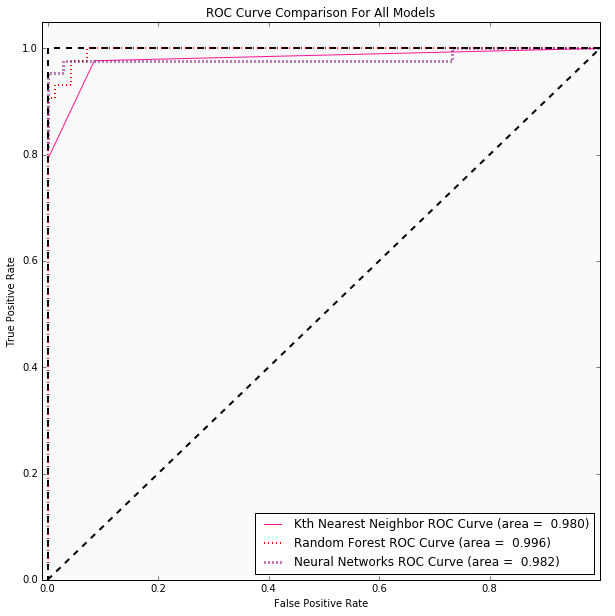 69 |
70 | #### ROC Curves zoomed in
71 |
69 |
70 | #### ROC Curves zoomed in
71 | 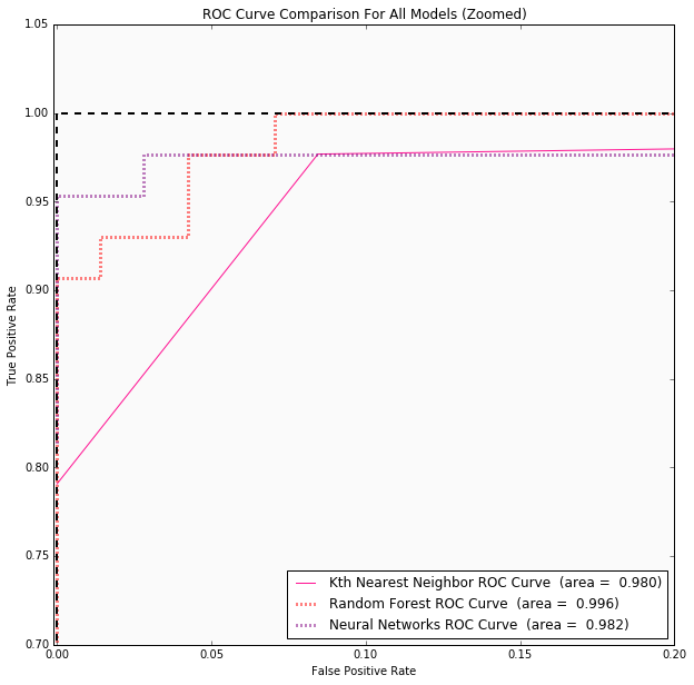 72 |
73 | The ROC Curves are more telling of **Random Forest** being a better model for predicting.
74 |
75 | Any feedback is welcomed!
76 |
77 | Things to do:
78 | + Create **Jupyter Notebook** for *KNN* and *NN* (1/25/2018)
79 | + Unit test scripts
80 |
--------------------------------------------------------------------------------
/src/python/random_forest.py:
--------------------------------------------------------------------------------
1 | #!/usr/bin/env python3
2 |
3 | #####################################################
4 | ## WISCONSIN BREAST CANCER - MACHINE LEARNING ##
5 | #####################################################
6 | #
7 | # Project by Raul Eulogio
8 | #
9 | # Project found at: https://www.inertia7.com/projects/3
10 | #
11 |
12 | """
13 | Random Forest Classification
14 | """
15 | # Import Packages -----------------------------------------------
16 | import time
17 | import sys
18 | from numpy import argsort
19 | import pandas as pd
20 | import helper_functions as hf
21 | from data_extraction import names_index
22 | from data_extraction import training_set, class_set
23 | from data_extraction import test_set, test_class_set
24 | from sklearn.ensemble import RandomForestClassifier
25 | from produce_model_metrics import produce_model_metrics
26 |
27 | # Fitting Random Forest -----------------------------------------
28 | # Set the random state for reproducibility
29 | fit_rf = RandomForestClassifier(random_state=42)
30 |
31 | ## Set best parameters given by grid search
32 | fit_rf.set_params(criterion = 'gini',
33 | max_features = 'log2',
34 | max_depth = 3,
35 | n_estimators=400)
36 |
37 | # Fit model on training data
38 | fit_rf.fit(training_set,
39 | class_set)
40 |
41 | # Tree Specific -------------------------------------------------
42 |
43 | # Extracting feature importance
44 | var_imp_rf = hf.variable_importance(fit_rf)
45 |
46 | importances_rf = var_imp_rf['importance']
47 |
48 | indices_rf = var_imp_rf['index']
49 |
50 | if __name__=='__main__':
51 | # Print model parameters ------------------------------------
52 | print(fit_rf, '\n')
53 |
54 | # Initialize function for metrics ---------------------------
55 | fit_dict_rf = produce_model_metrics(fit_rf,
56 | test_set,
57 | test_class_set,
58 | 'rf')
59 |
60 | # Extract each piece from dictionary
61 | predictions_rf = fit_dict_rf['predictions']
62 | accuracy_rf = fit_dict_rf['accuracy']
63 | auc_rf = fit_dict_rf['auc']
64 |
65 | print("Hyperparameter Optimization:")
66 | print("chosen parameters: \n \
67 | {'max_features': 'log2', \n \
68 | 'max_depth': 3, \n \
69 | 'bootstrap': True, \n \
70 | 'criterion': 'gini'}")
71 | print("Note: Remove commented code to see this section \n")
72 |
73 | # np.random.seed(42)
74 | # start = time.time()
75 | # param_dist = {'max_depth': [2, 3, 4],
76 | # 'bootstrap': [True, False],
77 | # 'max_features': ['auto', 'sqrt',
78 | # 'log2', None],
79 | # 'criterion': ['gini', 'entropy']}
80 | # cv_rf = GridSearchCV(fit_rf, cv = 10,
81 | # param_grid=param_dist,
82 | # n_jobs = 3)
83 | # cv_rf.fit(training_set, class_set)
84 | # print('Best Parameters using grid search: \n',
85 | # cv_rf.best_params_)
86 | # end = time.time()
87 | # print('Time taken in grid search: {0: .2f}'\
88 | #.format(end - start))
89 |
90 | # Test Set Calculations -------------------------------------
91 | # Test error rate
92 | test_error_rate_rf = 1 - accuracy_rf
93 |
94 | # Confusion Matrix
95 | test_crosstb = hf.create_conf_mat(test_class_set,
96 | predictions_rf)
97 |
98 | # Print Variable Importance
99 | hf.print_var_importance(importances_rf, indices_rf, names_index)
100 |
101 | # Cross validation
102 | print('Cross Validation:')
103 | hf.cross_val_metrics(fit_rf,
104 | training_set,
105 | class_set,
106 | 'rf',
107 | print_results = True)
108 |
109 | print('Confusion Matrix:')
110 | print(test_crosstb, '\n')
111 |
112 | print("Here is our mean accuracy on the test set:\n {0: 0.3f}"\
113 | .format(accuracy_rf))
114 |
115 | print("The test error rate for our model is:\n {0: .3f}"\
116 | .format(test_error_rate_rf))
117 | import pdb
118 | pdb.set_trace()
119 |
--------------------------------------------------------------------------------
/src/r/random_forest.R:
--------------------------------------------------------------------------------
1 |
2 | # Load Packages
3 | suppressWarnings(library(tidyverse))
4 | suppressWarnings(library(caret))
5 | suppressWarnings(library(ggcorrplot))
6 | suppressWarnings(library(GGally))
7 | suppressWarnings(library(randomForest))
8 | suppressWarnings(library(e1071))
9 | suppressWarnings(library(ROCR))
10 | suppressWarnings(library(pROC))
11 | suppressWarnings(library(RCurl))
12 | library(here)
13 |
14 | # Load Data
15 | UCI_data_URL <- getURL('https://archive.ics.uci.edu/ml/machine-learning-databases/breast-cancer-wisconsin/wdbc.data')
16 | names <- c('id_number', 'diagnosis', 'radius_mean',
17 | 'texture_mean', 'perimeter_mean', 'area_mean',
18 | 'smoothness_mean', 'compactness_mean',
19 | 'concavity_mean','concave_points_mean',
20 | 'symmetry_mean', 'fractal_dimension_mean',
21 | 'radius_se', 'texture_se', 'perimeter_se',
22 | 'area_se', 'smoothness_se', 'compactness_se',
23 | 'concavity_se', 'concave_points_se',
24 | 'symmetry_se', 'fractal_dimension_se',
25 | 'radius_worst', 'texture_worst',
26 | 'perimeter_worst', 'area_worst',
27 | 'smoothness_worst', 'compactness_worst',
28 | 'concavity_worst', 'concave_points_worst',
29 | 'symmetry_worst', 'fractal_dimension_worst')
30 | breast_cancer <- read.table(textConnection(UCI_data_URL), sep = ',', col.names = names)
31 |
32 | breast_cancer$id_number <- NULL
33 |
34 | # Preview Data
35 | head(breast_cancer)
36 |
37 | # Structure of data
38 | breast_cancer %>%
39 | dim()
40 | breast_cancer %>%
41 | str()
42 |
43 | # Check distribution of Class
44 | breast_cancer %>%
45 | count(diagnosis) %>%
46 | group_by(diagnosis) %>%
47 | summarize(perc_dx = round((n / 569)* 100, 2))
48 |
49 | summary(breast_cancer)
50 |
51 | # Create Training and Test Set
52 | set.seed(42)
53 | trainIndex <- createDataPartition(breast_cancer$diagnosis,
54 | p = .8,
55 | list = FALSE,
56 | times = 1)
57 | training_set <- breast_cancer[ trainIndex, ]
58 | test_set <- breast_cancer[ -trainIndex, ]
59 |
60 | # Custom grid search
61 | # From https://machinelearningmastery.com/tune-machine-learning-algorithms-in-r/
62 | customRF <- list(type = "Classification", library = "randomForest", loop = NULL)
63 | customRF$parameters <- data.frame(parameter = c("mtry", "ntree", "nodesize"), class = rep("numeric", 3), label = c("mtry", "ntree", "nodesize"))
64 | customRF$grid <- function(x, y, len = NULL, search = "grid") {}
65 | customRF$fit <- function(x, y, wts, param, lev, last, weights, classProbs, ...) {
66 | randomForest(x, y, mtry = param$mtry, ntree=param$ntree, nodesize=param$nodesize, ...)
67 | }
68 | customRF$predict <- function(modelFit, newdata, preProc = NULL, submodels = NULL)
69 | predict(modelFit, newdata)
70 | customRF$prob <- function(modelFit, newdata, preProc = NULL, submodels = NULL)
71 | predict(modelFit, newdata, type = "prob")
72 | customRF$sort <- function(x) x[order(x[,1]),]
73 | customRF$levels <- function(x) x$classes
74 |
75 | # Fitting Model
76 | fitControl <- trainControl(## 10-fold CV
77 | method = "repeatedcv",
78 | number = 3,
79 | ## repeated ten times
80 | repeats = 10)
81 |
82 | grid <- expand.grid(.mtry=c(floor(sqrt(ncol(training_set))), (ncol(training_set) - 1), floor(log(ncol(training_set)))),
83 | .ntree = c(100, 300, 500, 1000),
84 | .nodesize =c(1:4))
85 | set.seed(42)
86 | fit_rf <- train(as.factor(diagnosis) ~ .,
87 | data = training_set,
88 | method = customRF,
89 | metric = "Accuracy",
90 | tuneGrid= grid,
91 | trControl = fitControl)
92 |
93 | # Final Model
94 | fit_rf$finalModel
95 |
96 | # Diangostic Plots
97 | fit_rf
98 |
99 | suppressWarnings(ggplot(fit_rf) +
100 | theme_bw() +
101 | ggtitle('Line plot for Random Forest'))
102 |
103 | # Variable Importance
104 | varImportance <- varImp(fit_rf, scale = FALSE)
105 |
106 | varImportanceScores <- data.frame(varImportance$importance)
107 |
108 | varImportanceScores <- data.frame(names = row.names(varImportanceScores), var_imp_scores = varImportanceScores$B)
109 |
110 | varImportanceScores
111 |
112 | # Visual
113 | ggplot(varImportanceScores,
114 | aes(reorder(names, var_imp_scores), var_imp_scores)) +
115 | geom_bar(stat='identity',
116 | fill = '#875FDB') +
117 | theme(panel.background = element_rect(fill = '#fafafa')) +
118 | coord_flip() +
119 | labs(x = 'Feature', y = 'Importance') +
120 | ggtitle('Feature Importance for Random Forest Model')
121 | ggplot(varImportanceScores,
122 | aes(reorder(names, var_imp_scores), var_imp_scores)) +
123 | geom_bar(stat='identity',
124 | fill = '#875FDB') +
125 | theme(panel.background = element_rect(fill = '#fafafa')) +
126 | coord_flip() +
127 | labs(x = 'Feature', y = 'Importance') +
128 | ggtitle('Feature Importance for Random Forest Model')
129 |
130 | # Out of Bag Error Rate
131 | oob_error <- data.frame(mtry = seq(1:100), oob = fit_rf$finalModel$err.rate[, 'OOB'])
132 |
133 | paste0('Out of Bag Error Rate for model is: ', round(oob_error[100, 2], 4))
134 |
135 | ggplot(oob_error, aes(mtry, oob)) +
136 | geom_line(colour = 'red') +
137 | theme_minimal() +
138 | ggtitle('OOB Error Rate across 100 trees') +
139 | labs(y = 'OOB Error Rate')
140 |
141 | # Test Set Predictions
142 | predict_values <- predict(fit_rf, newdata = test_set)
--------------------------------------------------------------------------------
/src/r/breastCancer.R:
--------------------------------------------------------------------------------
1 | # LOAD PACKAGES
2 | setwd('/home/rxe/myProjects/breastCancer/scripts/r')
3 |
4 | require(tidyverse)
5 | require(caret)
6 | require(ggcorrplot)
7 | require(GGally)
8 | require(class)
9 | require(randomForest)
10 | require(nnet)
11 | require(e1071)
12 | require(pROC)
13 | require(class)
14 |
15 | # EXPLORATORY ANALYSIS
16 | breastCancer <- read_csv('wdbc.data.txt')
17 | breast_simp <- read_csv('breast_cancer.txt')
18 |
19 | View(inner_join(breastCancer, breast_simp, by = "id_number"))
20 |
21 | head(breastCancer)
22 | dim(breastCancer)
23 |
24 | # REMOVING 'id_number'
25 | breastCancer$id_number <- NULL
26 |
27 | table(breastCancer$diagnosis)
28 | summary(breastCancer)
29 |
30 | # Scatterplot Matrix
31 | p <- ggpairs(data = breastCancer,
32 | columns = c('concave_points_worst', 'concavity_mean',
33 | 'perimeter_worst', 'radius_worst',
34 | 'area_worst', 'diagnosis'),
35 | mapping = aes(color = diagnosis)) +
36 | theme(panel.background = element_rect(fill = '#fafafa')) +
37 | ggtitle('Scatter Plot Matrix')
38 |
39 | # MANUALLY CHANGING COLORS OF PLOT
40 | # BORROWED FROM: https://stackoverflow.com/questions/34740210/how-to-change-the-color-palette-for-ggallyggpairs
41 | for(i in 1:p$nrow) {
42 | for(j in 1:p$ncol){
43 | p[i,j] <- p[i,j] +
44 | scale_fill_manual(values=c("red", "#875FDB")) +
45 | scale_color_manual(values=c("red", "#875FDB"))
46 | }
47 | }
48 |
49 | p
50 | # Pearson Correlation
51 | corr <- round(cor(breastCancer[, 2:31]), 2)
52 | ggcorrplot(corr,
53 | colors = c('red', 'white', '#875FDB')) +
54 | ggtitle('Peasron Correlation Matrix')
55 |
56 | # Box Plot
57 | ggplot(data = stack(breastCancer),
58 | aes(x = ind, y = values)) +
59 | geom_boxplot() +
60 | coord_flip(ylim = c(-.05, 50)) +
61 | theme(panel.background = element_rect(fill = '#fafafa')) +
62 | ggtitle('Box Plot of Unprocessed Data')
63 |
64 | # NORMALIZING
65 | preprocessparams <- preProcess(breastCancer[, 3:31], method=c('range'))
66 |
67 | breastCancerNorm <- predict(preprocessparams, breastCancer[, 3:31])
68 |
69 | breastCancerNorm <- data.table(breastCancerNorm, diangosis = breastCancer$diagnosis)
70 |
71 | summary(breastCancerNorm)
72 | # Box Plot of Normalized data
73 | ggplot(data = stack(breastCancerNorm),
74 | aes(x = ind, y = values)) +
75 | geom_boxplot() +
76 | coord_flip(ylim = c(-.05, 1.05)) +
77 | theme(panel.background = element_rect(fill = '#fafafa')) +
78 | ggtitle('Box Plot of Normalized Data')
79 |
80 | # TRAINING AND TEST SET
81 | breastCancer$diagnosis <- gsub('M', 1, breastCancer$diagnosis)
82 | breastCancer$diagnosis <- gsub('B', 0, breastCancer$diagnosis)
83 |
84 | breastCancer$diagnosis <- as.numeric(breastCancer$diagnosis)
85 |
86 | set.seed(42)
87 | trainIndex <- createDataPartition(breastCancer$diagnosis,
88 | p = .8,
89 | list = FALSE,
90 | times = 1)
91 |
92 | training_set <- breastCancer[ trainIndex, ]
93 | test_set <- breastCancer[ -trainIndex, ]
94 | ## Kth Nearest Neighbor
95 |
96 | # TRAINING AND TEST SETS ARE SET UP DIFFERENTLY FOR KNN
97 | # SO HERE WE'RE DOING THAT
98 | # Intialize a class set as vector
99 | class_set <- as.vector(training_set$diagnosis)
100 |
101 | test_set_knn <- test_set
102 | training_set_knn <- training_set
103 | test_set_knn$diagnosis <- NULL
104 | training_set_knn$diagnosis <- NULL
105 |
106 | head(test_set_knn)
107 |
108 | # FITTING MODEL
109 | fit_knn <- knn(training_set_knn, test_set_knn, class_set, k = 7)
110 |
111 | # TEST SET EVALUATIONS
112 | table(test_set$diagnosis, fit_knn)
113 |
114 | # TEST ERROR RATE: 0.063
115 |
116 | ## RANDOM FOREST
117 | # FITTING MODEL
118 | fitControl <- trainControl(## 10-fold CV
119 | method = "repeatedcv",
120 | number = 10,
121 | ## repeated ten times
122 | repeats = 10)
123 |
124 | set.seed(42)
125 | fit_rf <- train(as.factor(diagnosis) ~ .,
126 | data = training_set,
127 | method = "rf",
128 | trControl = fitControl)
129 |
130 | fit_rf$finalModel
131 |
132 | # VARIABLE IMPORTANCE
133 | varImportance <- varImp(fit_rf, scale = FALSE)
134 |
135 | varImportanceScores <- data.table(varImportance$importance, names = colnames(breastCancer[, 2:31]))
136 |
137 | varImportanceScores
138 |
139 | # VISUAL OF VARIABLE IMPORTANCE
140 | ggplot(varImportanceScores,
141 | aes(reorder(names, Overall), Overall)) +
142 | geom_bar(stat='identity',
143 | fill = '#875FDB') +
144 | theme(panel.background = element_rect(fill = '#fafafa')) +
145 | coord_flip() +
146 | labs(x = 'Feature', y = 'Importance') +
147 | ggtitle('Feature Importance for Random Forest Model')
148 |
149 | # TEST SET EVALUATIONS
150 | predict_values <- predict(fit_rf, newdata = test_set)
151 |
152 | table(predict_values, test_set$diagnosis)
153 |
154 | # TEST ERROR RATE: 0.027
155 |
156 | # NEURAL NETWORKS
157 |
158 | # CREATING NORMALIZED TRAINING AND TEST SET
159 | set.seed(42)
160 | trainIndex_norm <- createDataPartition(breastCancerNorm$diangosis,
161 | p = .8,
162 | list = FALSE,
163 | times = 1)
164 |
165 | training_set_norm <- breastCancerNorm[ trainIndex, ]
166 | test_set_norm <- breastCancerNorm[ -trainIndex, ]
167 |
168 | training_set_norm
169 |
170 | fit_nn <- train(as.factor(diangosis) ~ .,
171 | data = training_set_norm,
172 | method = "nnet",
173 | hidden = 3,
174 | algorithm = 'backprop')
175 |
176 | fit_nn$finalModel
177 | plot(fit_nn)
178 | predict_val_nn <- predict(fit_nn, newdata = test_set_norm)
179 |
180 | table(predict_val_nn, test_set$diagnosis)
181 |
182 | # TEST ERROR RATE: 0.035
--------------------------------------------------------------------------------
/src/pyspark/breast_cancer_df.py:
--------------------------------------------------------------------------------
1 | # Load packages
2 | from pyspark.sql.functions import col
3 | from pyspark.ml.classification import RandomForestClassifier
4 | from pyspark.ml.classification import DecisionTreeClassifier
5 | from pyspark.ml.classification import MultilayerPerceptronClassifier
6 | from pyspark.ml.feature import StringIndexer
7 | from pyspark.ml.feature import MinMaxScaler
8 | from pyspark.ml.feature import VectorAssembler
9 | from pyspark.ml.evaluation import MulticlassClassificationEvaluator
10 | from pyspark.ml.classification import MultilayerPerceptronClassifier
11 |
12 |
13 | rdd = sc.textFile('data/data.txt').map(lambda lines: lines.split(" "))
14 |
15 | df = rdd.toDF()
16 |
17 | data = df.selectExpr('_1 as label', '_2 as radius_mean',
18 | '_3 as texture_mean', '_4 as perimeter_mean',
19 | '_5 as area_mean', '_6 as smoothness_mean',
20 | '_7 as compactness_mean', '_8 as concavity_mean',
21 | '_9 as concave_points_mean', '_10 as symmetry_mean',
22 | '_11 as fractal_dimension_mean', '_12 as radius_se',
23 | '_13 as texture_se', '_14 as perimeter_se',
24 | '_15 as area_se', '_16 as smoothness_se',
25 | '_17 as compactness_se', '_18 as concavity_se',
26 | '_19 as concave_points_se', '_20 as symmetry_se',
27 | '_21 as fractal_dimension_se', '_22 as radius_worst',
28 | '_23 as texture_worst', '_24 as perimeter_worst',
29 | '_25 as area_worst', '_26 as smoothness_worst',
30 | '_27 as compactness_worst', '_28 as concavity_worst',
31 | '_29 as concave_points_worst', '_30 as symmetry_worst',
32 | '_31 as fractal_dimension_worst')
33 |
34 |
35 | # Converting to correct data types
36 | newData = data.select([col(c).cast('float') if c != 'label' else col(c).cast('int') for c in data.columns ])
37 |
38 | # For loops to output the describe functionality neatly
39 | mylist = []
40 | mylist2 = []
41 | for i in range(0, 31):
42 | if (i % 2 != 0):
43 | mylist.append(newData.columns[i])
44 | else:
45 | mylist2.append(newData.columns[i])
46 |
47 | # Now we use the newly created lists that have even and odd columns respectively
48 | # to see some basic statistics for our dataset
49 | for i in range(0, 15):
50 | newData.describe(mylist[i], mylist2[i]).show()
51 |
52 | # Important meta-data inputting for when I start running models!
53 | # Meta-data for the feature space
54 | featureIndexer = VectorAssembler(
55 | inputCols = [x for x in newData.columns if x != 'label'],
56 | outputCol = 'features')
57 |
58 | df = featureIndexer.transform(newData)
59 |
60 | # Some tests to see if things came out properly
61 | df.select(df['features']).show()
62 | df.select(df['label']).show()
63 |
64 | # Creating training and test sets
65 | (trainingSet, testSet) = df.randomSplit([0.7, 0.3])
66 |
67 | ####################
68 | ## DECISION TREES ##
69 | ####################
70 |
71 | # Creating training and test sets
72 |
73 | dt = DecisionTreeClassifier(labelCol="label",
74 | featuresCol = "features")
75 |
76 | #pipeline_dt = Pipeline(stages=[labelIndexer0, featureIndexer0, dt])
77 |
78 | model_dt = dt.fit(trainingSet)
79 |
80 | predictions_dt = model_dt.transform(testSet)
81 |
82 | # Select example rows to display.
83 | predictions_dt.select("prediction",
84 | "label",
85 | "features").show(5)
86 |
87 | # Select (prediction, true label) and compute test error
88 | evaluator_dt = MulticlassClassificationEvaluator(
89 | labelCol="label",
90 | predictionCol="prediction",
91 | metricName="accuracy")
92 |
93 | accuracy_dt = evaluator_dt.evaluate(predictions_dt)
94 |
95 | print("Test Error = %g " % (1.0 - accuracy_dt))
96 | '''
97 | Test Error = 0.0697674
98 | '''
99 |
100 | #########################
101 | ## Random Forest Model ##
102 | #########################
103 |
104 | rf = RandomForestClassifier(labelCol='label',
105 | maxDepth=4,
106 | impurity="gini",
107 | numTrees=500,
108 | seed=42)
109 |
110 | model_rf = rf.fit(trainingSet)
111 |
112 | predictions_rf = model_rf.transform(testSet)
113 |
114 | predictions_rf.select("prediction", "label", "features").show(10)
115 |
116 | '''
117 | +----------+-----+--------------------+
118 | |prediction|label| features|
119 | +----------+-----+--------------------+
120 | | 0.0| 0|[0.0,0.1258031932...|
121 | | 0.0| 0|[0.05859245005374...|
122 | | 0.0| 0|[0.07652986773450...|
123 | | 0.0| 0|[0.07747645570059...|
124 | | 0.0| 0|[0.07998483256627...|
125 | | 0.0| 0|[0.09025507729212...|
126 | | 0.0| 0|[0.09318944582402...|
127 | | 0.0| 0|[0.11756354432107...|
128 | | 0.0| 0|[0.11940932766481...|
129 | | 0.0| 0|[0.13280324046146...|
130 | +----------+-----+--------------------+
131 | only showing top 10 rows
132 | '''
133 |
134 | evaluator_rf = MulticlassClassificationEvaluator(labelCol="label",
135 | predictionCol="prediction",
136 | metricName="accuracy")
137 |
138 | accuracy_rf = evaluator_rf.evaluate(predictions_rf)
139 | print("Test Error = %g" % (1.0 - accuracy_rf))
140 | '''
141 | Test Error = 0.0223
142 | '''
143 |
144 | #####################
145 | ## NEURAL NETWORKS ##
146 | #####################
147 |
148 | ########################
149 | ## RESCALING DATA SET ##
150 | ########################
151 | # Typically for Neural Networks to perform better
152 | # a lot of preprocessing has to go into the data
153 | # So I scaled the feature space to have min = 0 and max = 1
154 |
155 | scaler = MinMaxScaler(inputCol='features', outputCol='scaledFeatures')
156 |
157 | scalerModel = scaler.fit(df)
158 |
159 | scaledData = scalerModel.transform(df)
160 |
161 | print("Features scaled to range: [%f, %f]" % (scaler.getMin(), scaler.getMax()))
162 |
163 | scaledData.select("features", "scaledFeatures").show()
164 |
165 | new_df = scaledData.selectExpr("label", "radius_mean", "texture_mean",
166 | "perimeter_mean", "area_mean", "smoothness_mean", "compactness_mean",
167 | "concavity_mean", "concave_points_mean", "symmetry_mean",
168 | "fractal_dimension_mean", "radius_se", "texture_se", "perimeter_se",
169 | "area_se", "smoothness_se", "compactness_se", "concavity_se",
170 | "concave_points_se", "symmetry_se", "fractal_dimension_se",
171 | "radius_worst", "texture_worst", "perimeter_worst",
172 | "area_worst", "smoothness_worst", "compactness_worst",
173 | "concavity_worst", "concave_points_worst", "symmetry_worst",
174 | "fractal_dimension_worst","features as oldFeature",
175 | "scaledFeatures as features")
176 |
177 | # Creating training and test sets
178 | (trainingSet_scaled, testSet_scaled) = new_df\
179 | .randomSplit([0.7, 0.3])
180 |
181 | layers = [30, 5, 4, 2]
182 |
183 | trainer = MultilayerPerceptronClassifier(maxIter=100,
184 | layers=layers,
185 | blockSize=128,
186 | seed=1234)
187 |
188 | model_nn = trainer.fit(trainingSet_scaled)
189 |
190 | result_nn = model_nn.transform(testSet_scaled)
191 | predictions_nn = result_nn.select("prediction", "label")
192 | evaluator_nn = MulticlassClassificationEvaluator(metricName="accuracy")
193 |
194 | accuracy_nn = evaluator_nn.evaluate(predictions_nn)
195 |
196 | print("Test Error = %g" % (1.0 - accuracy_nn))
197 | '''
198 | Test Error = 0.0314465
199 | '''
--------------------------------------------------------------------------------
/src/python/model_eval.py:
--------------------------------------------------------------------------------
1 | #!/usr/bin/env python3
2 |
3 | #####################################################
4 | ## WISCONSIN BREAST CANCER MACHINE LEARNING ##
5 | #####################################################
6 |
7 | # Project by Raul Eulogio
8 |
9 | # Project found at: https://www.inertia7.com/projects/3
10 |
11 |
12 | """
13 | Model Evaluation
14 | """
15 | # Import Packages -----------------------------------------------
16 | import matplotlib.pyplot as plt
17 | from knn import fit_knn
18 | from random_forest import fit_rf
19 | from neural_networks import fit_nn
20 | from data_extraction import training_set, class_set
21 | from data_extraction import test_set, test_class_set
22 | from data_extraction import training_set_scaled, test_set_scaled
23 | from helper_functions import cross_val_metrics
24 | from produce_model_metrics import produce_model_metrics
25 | from terminaltables import AsciiTable
26 | from sklearn.metrics import classification_report
27 |
28 |
29 |
30 | # Calling up metrics from the model scripts
31 | # KNN -----------------------------------------------------------
32 | metrics_knn = produce_model_metrics(fit_knn, test_set,
33 | test_class_set, 'knn')
34 | # Call each value from dictionary
35 | predictions_knn = metrics_knn['predictions']
36 | accuracy_knn = metrics_knn['accuracy']
37 | fpr = metrics_knn['fpr']
38 | tpr = metrics_knn['tpr']
39 | auc_knn = metrics_knn['auc']
40 |
41 | # Test Error Rate
42 | test_error_rate_knn = 1 - accuracy_knn
43 |
44 | # Cross Validated Score
45 | mean_cv_knn, std_error_knn = cross_val_metrics(fit_knn,
46 | training_set,
47 | class_set,
48 | 'knn',
49 | print_results = False)
50 |
51 | # RF ------------------------------------------------------------
52 | metrics_rf = produce_model_metrics(fit_rf, test_set,
53 | test_class_set, 'rf')
54 | # Call each value from dictionary
55 | predictions_rf = metrics_rf['predictions']
56 | accuracy_rf = metrics_rf['accuracy']
57 | fpr2 = metrics_rf['fpr']
58 | tpr2 = metrics_rf['tpr']
59 | auc_rf = metrics_rf['auc']
60 |
61 | # Test Error Rate
62 | test_error_rate_rf = 1 - accuracy_rf
63 |
64 | # Cross Validated Score
65 | mean_cv_rf, std_error_rf = cross_val_metrics(fit_rf,
66 | training_set,
67 | class_set,
68 | 'rf',
69 | print_results = False)
70 |
71 | # NN ------------------------------------------------------------
72 | metrics_nn = produce_model_metrics(fit_nn, test_set_scaled,
73 | test_class_set, 'nn')
74 |
75 | # Call each value from dictionary
76 | predictions_nn = metrics_nn['predictions']
77 | accuracy_nn = metrics_nn['accuracy']
78 | fpr3 = metrics_nn['fpr']
79 | tpr3 = metrics_nn['tpr']
80 | auc_nn = metrics_nn['auc']
81 |
82 | # Test Error Rate
83 | test_error_rate_nn = 1 - accuracy_nn
84 |
85 | # Cross Validated Score
86 | mean_cv_nn, std_error_nn = cross_val_metrics(fit_nn,
87 | training_set_scaled,
88 | class_set,
89 | 'nn',
90 | print_results = False)
91 |
92 | # Main ----------------------------------------------------------
93 | if __name__ == '__main__':
94 | # Populate list for human readable table from terminal line
95 | table_data = [[ 'Model/Algorithm', 'Test Error Rate',
96 | 'False Negative for Test Set', 'Area under the Curve for ROC',
97 | 'Cross Validation Score'],
98 | ['Kth Nearest Neighbor',
99 | round(test_error_rate_knn, 3),
100 | 5,
101 | round(auc_knn, 3),
102 | "Accuracy: {0: 0.3f} (+/- {1: 0.3f})"\
103 | .format(mean_cv_knn, std_error_knn)],
104 | [ 'Random Forest',
105 | round(test_error_rate_rf, 3),
106 | 3,
107 | round(auc_rf, 3),
108 | "Accuracy: {0: 0.3f} (+/- {1: 0.3f})"\
109 | .format(mean_cv_rf, std_error_rf)],
110 | [ 'Neural Networks' ,
111 | round(test_error_rate_nn, 3),
112 | 1,
113 | round(auc_nn, 3),
114 | "Accuracy: {0: 0.3f} (+/- {1: 0.3f})"\
115 | .format(mean_cv_nn, std_error_nn)]]
116 |
117 | # convert to AsciiTable from terminaltables package
118 | table = AsciiTable(table_data)
119 |
120 | target_names = ['Benign', 'Malignant']
121 |
122 | print('Classification Report for Kth Nearest Neighbor:')
123 | print(classification_report(predictions_knn,
124 | test_class_set,
125 | target_names = target_names))
126 |
127 | print('Classification Report for Random Forest:')
128 | print(classification_report(predictions_rf,
129 | test_class_set,
130 | target_names = target_names))
131 |
132 | print('Classification Report for Neural Networks:')
133 | print(classification_report(predictions_nn,
134 | test_class_set,
135 | target_names = target_names))
136 |
137 | print("Comparison of different logistics relating to model evaluation:")
138 | print(table.table)
139 |
140 | # Plotting ROC Curves----------------------------------------
141 | f, ax = plt.subplots(figsize=(10, 10))
142 |
143 | plt.plot(fpr, tpr, label='Kth Nearest Neighbor ROC Curve (area = {0: .3f})'\
144 | .format(auc_knn),
145 | color = 'deeppink',
146 | linewidth=1)
147 | plt.plot(fpr2, tpr2,label='Random Forest ROC Curve (area = {0: .3f})'\
148 | .format(auc_rf),
149 | color = 'red',
150 | linestyle=':',
151 | linewidth=2)
152 | plt.plot(fpr3, tpr3,label='Neural Networks ROC Curve (area = {0: .3f})'\
153 | .format(auc_nn),
154 | color = 'purple',
155 | linestyle=':',
156 | linewidth=3)
157 |
158 | ax.set_axis_bgcolor('#fafafa')
159 | plt.plot([0, 1], [0, 1], 'k--', lw=2)
160 | plt.plot([0, 0], [1, 0], 'k--', lw=2, color = 'black')
161 | plt.plot([1, 0], [1, 1], 'k--', lw=2, color = 'black')
162 | plt.xlim([-0.01, 1.0])
163 | plt.ylim([0.0, 1.05])
164 | plt.xlabel('False Positive Rate')
165 | plt.ylabel('True Positive Rate')
166 | plt.title('ROC Curve Comparison For All Models')
167 | plt.legend(loc="lower right")
168 | plt.show()
169 |
170 | # Zoomed in
171 | f, ax = plt.subplots(figsize=(10, 10))
172 | plt.plot(fpr, tpr, label='Kth Nearest Neighbor ROC Curve (area = {0: .3f})'\
173 | .format(auc_knn),
174 | color = 'deeppink',
175 | linewidth=1)
176 | plt.plot(fpr2, tpr2,label='Random Forest ROC Curve (area = {0: .3f})'\
177 | .format(auc_rf),
178 | color = 'red',
179 | linestyle=':',
180 | linewidth=3)
181 | plt.plot(fpr3, tpr3,label='Neural Networks ROC Curve (area = {0: .3f})'\
182 | .format(auc_nn),
183 | color = 'purple',
184 | linestyle=':',
185 | linewidth=3)
186 |
187 | ax.set_axis_bgcolor('#fafafa')
188 | plt.plot([0, 1], [0, 1], 'k--', lw=2) # Add Diagonal line
189 | plt.plot([0, 0], [1, 0], 'k--', lw=2, color = 'black')
190 | plt.plot([1, 0], [1, 1], 'k--', lw=2, color = 'black')
191 | plt.xlim([-0.001, 0.2])
192 | plt.ylim([0.7, 1.05])
193 | plt.xlabel('False Positive Rate')
194 | plt.ylabel('True Positive Rate')
195 | plt.title('ROC Curve Comparison For All Models (Zoomed)')
196 | plt.legend(loc="lower right")
197 | plt.show()
198 |
199 | print('fin \n:)')
200 |
--------------------------------------------------------------------------------
/src/r/packrat/init.R:
--------------------------------------------------------------------------------
1 | local({
2 |
3 | ## Helper function to get the path to the library directory for a
4 | ## given packrat project.
5 | getPackratLibDir <- function(projDir = NULL) {
6 | path <- file.path("packrat", "lib", R.version$platform, getRversion())
7 |
8 | if (!is.null(projDir)) {
9 |
10 | ## Strip trailing slashes if necessary
11 | projDir <- sub("/+$", "", projDir)
12 |
13 | ## Only prepend path if different from current working dir
14 | if (!identical(normalizePath(projDir), normalizePath(getwd())))
15 | path <- file.path(projDir, path)
16 | }
17 |
18 | path
19 | }
20 |
21 | ## Ensure that we set the packrat library directory relative to the
22 | ## project directory. Normally, this should be the working directory,
23 | ## but we also use '.rs.getProjectDirectory()' if necessary (e.g. we're
24 | ## rebuilding a project while within a separate directory)
25 | libDir <- if (exists(".rs.getProjectDirectory"))
26 | getPackratLibDir(.rs.getProjectDirectory())
27 | else
28 | getPackratLibDir()
29 |
30 | ## Unload packrat in case it's loaded -- this ensures packrat _must_ be
31 | ## loaded from the private library. Note that `requireNamespace` will
32 | ## succeed if the package is already loaded, regardless of lib.loc!
33 | if ("packrat" %in% loadedNamespaces())
34 | try(unloadNamespace("packrat"), silent = TRUE)
35 |
36 | if (suppressWarnings(requireNamespace("packrat", quietly = TRUE, lib.loc = libDir))) {
37 |
38 | # Check 'print.banner.on.startup' -- when NA and RStudio, don't print
39 | print.banner <- packrat::get_opts("print.banner.on.startup")
40 | if (print.banner == "auto" && is.na(Sys.getenv("RSTUDIO", unset = NA))) {
41 | print.banner <- TRUE
42 | } else {
43 | print.banner <- FALSE
44 | }
45 | return(packrat::on(print.banner = print.banner))
46 | }
47 |
48 | ## Escape hatch to allow RStudio to handle bootstrapping. This
49 | ## enables RStudio to provide print output when automagically
50 | ## restoring a project from a bundle on load.
51 | if (!is.na(Sys.getenv("RSTUDIO", unset = NA)) &&
52 | is.na(Sys.getenv("RSTUDIO_PACKRAT_BOOTSTRAP", unset = NA))) {
53 | Sys.setenv("RSTUDIO_PACKRAT_BOOTSTRAP" = "1")
54 | setHook("rstudio.sessionInit", function(...) {
55 | # Ensure that, on sourcing 'packrat/init.R', we are
56 | # within the project root directory
57 | if (exists(".rs.getProjectDirectory")) {
58 | owd <- getwd()
59 | setwd(.rs.getProjectDirectory())
60 | on.exit(setwd(owd), add = TRUE)
61 | }
62 | source("packrat/init.R")
63 | })
64 | return(invisible(NULL))
65 | }
66 |
67 | ## Bootstrapping -- only performed in interactive contexts,
68 | ## or when explicitly asked for on the command line
69 | if (interactive() || "--bootstrap-packrat" %in% commandArgs(TRUE)) {
70 |
71 | message("Packrat is not installed in the local library -- ",
72 | "attempting to bootstrap an installation...")
73 |
74 | ## We need utils for the following to succeed -- there are calls to functions
75 | ## in 'restore' that are contained within utils. utils gets loaded at the
76 | ## end of start-up anyhow, so this should be fine
77 | library("utils", character.only = TRUE)
78 |
79 | ## Install packrat into local project library
80 | packratSrcPath <- list.files(full.names = TRUE,
81 | file.path("packrat", "src", "packrat")
82 | )
83 |
84 | ## No packrat tarballs available locally -- try some other means of installation
85 | if (!length(packratSrcPath)) {
86 |
87 | message("> No source tarball of packrat available locally")
88 |
89 | ## There are no packrat sources available -- try using a version of
90 | ## packrat installed in the user library to bootstrap
91 | if (requireNamespace("packrat", quietly = TRUE) && packageVersion("packrat") >= "0.2.0.99") {
92 | message("> Using user-library packrat (",
93 | packageVersion("packrat"),
94 | ") to bootstrap this project")
95 | }
96 |
97 | ## Couldn't find a user-local packrat -- try finding and using devtools
98 | ## to install
99 | else if (requireNamespace("devtools", quietly = TRUE)) {
100 | message("> Attempting to use devtools::install_github to install ",
101 | "a temporary version of packrat")
102 | library(stats) ## for setNames
103 | devtools::install_github("rstudio/packrat")
104 | }
105 |
106 | ## Try downloading packrat from CRAN if available
107 | else if ("packrat" %in% rownames(available.packages())) {
108 | message("> Installing packrat from CRAN")
109 | install.packages("packrat")
110 | }
111 |
112 | ## Fail -- couldn't find an appropriate means of installing packrat
113 | else {
114 | stop("Could not automatically bootstrap packrat -- try running ",
115 | "\"'install.packages('devtools'); devtools::install_github('rstudio/packrat')\"",
116 | "and restarting R to bootstrap packrat.")
117 | }
118 |
119 | # Restore the project, unload the temporary packrat, and load the private packrat
120 | packrat::restore(prompt = FALSE, restart = TRUE)
121 |
122 | ## This code path only reached if we didn't restart earlier
123 | unloadNamespace("packrat")
124 | requireNamespace("packrat", lib.loc = libDir, quietly = TRUE)
125 | return(packrat::on())
126 |
127 | }
128 |
129 | ## Multiple packrat tarballs available locally -- try to choose one
130 | ## TODO: read lock file and infer most appropriate from there; low priority because
131 | ## after bootstrapping packrat a restore should do the right thing
132 | if (length(packratSrcPath) > 1) {
133 | warning("Multiple versions of packrat available in the source directory;",
134 | "using packrat source:\n- ", shQuote(packratSrcPath))
135 | packratSrcPath <- packratSrcPath[[1]]
136 | }
137 |
138 |
139 | lib <- file.path("packrat", "lib", R.version$platform, getRversion())
140 | if (!file.exists(lib)) {
141 | dir.create(lib, recursive = TRUE)
142 | }
143 | lib <- normalizePath(lib, winslash = "/")
144 |
145 | message("> Installing packrat into project private library:")
146 | message("- ", shQuote(lib))
147 |
148 | surround <- function(x, with) {
149 | if (!length(x)) return(character())
150 | paste0(with, x, with)
151 | }
152 |
153 | ## The following is performed because a regular install.packages call can fail
154 | peq <- function(x, y) paste(x, y, sep = " = ")
155 | installArgs <- c(
156 | peq("pkgs", surround(packratSrcPath, with = "'")),
157 | peq("lib", surround(lib, with = "'")),
158 | peq("repos", "NULL"),
159 | peq("type", surround("source", with = "'"))
160 | )
161 | installCmd <- paste(sep = "",
162 | "utils::install.packages(",
163 | paste(installArgs, collapse = ", "),
164 | ")")
165 |
166 | fullCmd <- paste(
167 | surround(file.path(R.home("bin"), "R"), with = "\""),
168 | "--vanilla",
169 | "--slave",
170 | "-e",
171 | surround(installCmd, with = "\"")
172 | )
173 | system(fullCmd)
174 |
175 | ## Tag the installed packrat so we know it's managed by packrat
176 | ## TODO: should this be taking information from the lockfile? this is a bit awkward
177 | ## because we're taking an un-annotated packrat source tarball and simply assuming it's now
178 | ## an 'installed from source' version
179 |
180 | ## -- InstallAgent -- ##
181 | installAgent <- 'InstallAgent: packrat 0.4.8-1'
182 |
183 | ## -- InstallSource -- ##
184 | installSource <- 'InstallSource: source'
185 |
186 | packratDescPath <- file.path(lib, "packrat", "DESCRIPTION")
187 | DESCRIPTION <- readLines(packratDescPath)
188 | DESCRIPTION <- c(DESCRIPTION, installAgent, installSource)
189 | cat(DESCRIPTION, file = packratDescPath, sep = "\n")
190 |
191 | # Otherwise, continue on as normal
192 | message("> Attaching packrat")
193 | library("packrat", character.only = TRUE, lib.loc = lib)
194 |
195 | message("> Restoring library")
196 | restore(restart = FALSE)
197 |
198 | # If the environment allows us to restart, do so with a call to restore
199 | restart <- getOption("restart")
200 | if (!is.null(restart)) {
201 | message("> Packrat bootstrap successfully completed. ",
202 | "Restarting R and entering packrat mode...")
203 | return(restart())
204 | }
205 |
206 | # Callers (source-erers) can define this hidden variable to make sure we don't enter packrat mode
207 | # Primarily useful for testing
208 | if (!exists(".__DONT_ENTER_PACKRAT_MODE__.") && interactive()) {
209 | message("> Packrat bootstrap successfully completed. Entering packrat mode...")
210 | packrat::on()
211 | }
212 |
213 | Sys.unsetenv("RSTUDIO_PACKRAT_BOOTSTRAP")
214 |
215 | }
216 |
217 | })
218 |
--------------------------------------------------------------------------------
/dash_dashboard/app.py:
--------------------------------------------------------------------------------
1 | #!/usr/bin/env python3
2 |
3 | import sys
4 | import numpy as np
5 | import dash
6 | import dash_core_components as dcc
7 | import dash_html_components as html
8 | import plotly.graph_objs as go
9 | import global_vars as gv
10 | import pandas as pd
11 |
12 | sys.path.insert(0, '../src/python/')
13 | from data_extraction import breast_cancer, names
14 | sys.path.pop(0)
15 |
16 | # Test set metrics
17 | cross_tab_knn = gv.cross_tab_knn
18 | cross_tab_rf = gv.cross_tab_rf
19 | cross_tab_nn = gv.cross_tab_nn
20 |
21 | # Classification Reports
22 | class_rep_knn = gv.class_rep_knn
23 | class_rep_rf = gv.class_rep_rf
24 | class_rep_nn = gv.class_rep_nn
25 |
26 | def generate_table(dataframe, max_rows=10):
27 | return html.Table(
28 | # Header
29 | [html.Tr([html.Th(col) for col in dataframe.columns])] +
30 |
31 | # Body
32 | [html.Tr([
33 | html.Td(dataframe.iloc[i][col]) for col in dataframe.columns
34 | ]) for i in range(min(len(dataframe), max_rows))]
35 | )
36 |
37 | app = dash.Dash()
38 |
39 | app.layout = html.Div([
40 | html.Div([
41 | html.H2("Breast Cancer Dashboard"),
42 | ], className='banner'),
43 | html.H2(children = '''
44 | An interactive dashboard created by Raul Eulogio
45 | ''',
46 | style={
47 | 'padding': '0px 30px 15px 30px'}),
48 | html.Div([
49 | html.H3(children = '''
50 | Exploratory Analysis
51 | ''',
52 | style={
53 | 'padding': '0px 30px 15px 30px'})
54 | ]),
55 | html.Div([
56 | html.Div([
57 | html.P("""
58 | Move the multi-select options to see the 3d scatter plot and histograms change respectively.
59 | And play with the interactive 3d scatter plot to see how variables interact!
60 |
61 | """),
62 | html.Label('Choose the different parameters'),
63 | dcc.Dropdown(
64 | id='first_input',
65 | options=[
66 | {'label': i, 'value': i} for i in names[2:]
67 | ],
68 | value = 'area_worst'
69 | ),
70 | dcc.Dropdown(
71 | id='second_input',
72 | options=[
73 | {'label': i, 'value': i} for i in names[2:]
74 | ],
75 | value = 'perimeter_worst'
76 | ),
77 | dcc.Dropdown(
78 | id='third_input',
79 | options=[
80 | {'label': i, 'value': i} for i in names[2:]
81 | ],
82 | value = 'concave_points_worst'
83 | ),
84 | dcc.Graph(
85 | id='scatter_plot_3d'),
86 | html.Div(html.P(' .')),
87 | html.Div([
88 | html.H3("""
89 | Machine Learning
90 | """),
91 | dcc.Markdown('Here are some metrics relating to how well each model did.'),
92 | dcc.Markdown('+ See [this article](https://lukeoakdenrayner.wordpress.com/2017/12/06/do-machines-actually-beat-doctors-roc-curves-and-performance-metrics/) for more information about *ROC Curves* '),
93 | html.Label('Choose a Machine Learning Model'),
94 | dcc.Dropdown(
95 | id='machine_learning',
96 | options=[
97 | {'label': 'Kth Nearest Neighor', 'value': 'knn'},
98 | {'label': 'Random Forest', 'value': 'rf'},
99 | {'label': 'Neural Network', 'value': 'nn'}
100 | ],
101 | value = 'knn'
102 | ),
103 | dcc.Graph(
104 | id='roc_curve')
105 | ])
106 | ],
107 | style={'width': '40%',
108 | 'height': '50%',
109 | 'float': 'left',
110 | 'padding': '0px 40px 40px 40px'}),
111 | # End Left Side Div
112 | # Right Side Div
113 | html.Div([
114 | dcc.Graph(
115 | id='hist_first_var',
116 | style={'height': '12%'}
117 | ),
118 | dcc.Graph(
119 | id='hist_sec_var',
120 | style={'height': '12%'}
121 | ),
122 | dcc.Graph(
123 | id='hist_third_var',
124 | style={'height': '12%'}
125 | ),
126 | html.Div(html.P(' .')),
127 | html.Div(html.P(' .')),
128 | html.Div(html.P(' .')),
129 | html.Div(html.P(' .')),
130 | html.Div(
131 | html.H4("""
132 | Test Set Metrics
133 | """
134 | )
135 | ),
136 | dcc.Markdown("+ See [Test Set Metrics Section of inertia7 project](https://www.inertia7.com/projects/95#test_set_met) for more information."),
137 | html.Div(
138 | dcc.Graph(
139 | id="conf_mat",
140 | style={'height': '10%'}
141 | )
142 | ),
143 | html.Div(
144 | html.H4("""
145 | Classification Report
146 | """
147 | )),
148 | dcc.Markdown("+ See [Classification Report Section of inertia7 project](https://www.inertia7.com/projects/95) for more information. "),
149 | html.Div([html.Div(id='table_class_rep')
150 | ],
151 | style={'width': '100%'})
152 | ],
153 | style={'width': '40%',
154 | 'float': 'right',
155 | 'padding': '0px 40px 40px 40px'},
156 | )
157 | # End Right Side Div
158 | ],
159 | style={'width': '100%',
160 | 'height': '100%',
161 | 'display': 'flex'}),
162 | ])
163 |
164 | @app.callback(
165 | dash.dependencies.Output('scatter_plot_3d', 'figure'),
166 | [dash.dependencies.Input('first_input', 'value'),
167 | dash.dependencies.Input('second_input', 'value'),
168 | dash.dependencies.Input('third_input', 'value'),]
169 | )
170 |
171 | def update_figure(first_input_name, second_input_name, third_input_name):
172 | traces = []
173 | for i in breast_cancer.diagnosis.unique():
174 | breast_cancer_dx = breast_cancer[breast_cancer['diagnosis'] == i]
175 | if (i == 0):
176 | traces.append(go.Scatter3d(
177 | x=breast_cancer_dx[first_input_name],
178 | y=breast_cancer_dx[second_input_name],
179 | z=breast_cancer_dx[third_input_name],
180 | text=breast_cancer_dx['diagnosis'],
181 | mode='markers',
182 | opacity=0.7,
183 | marker={
184 | 'size': 15,
185 | 'line': {'width': 0.5, 'color': 'white'},
186 | 'color': 'red'
187 | },
188 | name='Malignant'
189 | ))
190 |
191 | else:
192 | traces.append(go.Scatter3d(
193 | x=breast_cancer_dx[first_input_name],
194 | y=breast_cancer_dx[second_input_name],
195 | z=breast_cancer_dx[third_input_name],
196 | text=breast_cancer_dx['diagnosis'],
197 | mode='markers',
198 | opacity=0.7,
199 | marker={
200 | 'size': 15,
201 | 'line': {'width': 0.5, 'color': 'white'},
202 | 'color': '#875FDB'
203 | },
204 | name='Benign'
205 | ))
206 | return {
207 | 'data': traces,
208 | 'layout': go.Layout(
209 | xaxis={'title': first_input_name},
210 | yaxis={'title': second_input_name},
211 | margin={'l': 40, 'b': 40, 't': 10, 'r': 10},
212 | legend={'x': 0, 'y': 1},
213 | hovermode='closest'
214 | )
215 | }
216 |
217 |
218 | @app.callback(
219 | dash.dependencies.Output('hist_first_var', 'figure'),
220 | [dash.dependencies.Input('first_input', 'value')]
221 | )
222 | def update_hist_1(first_input_name):
223 | traces_hist = []
224 | for i in breast_cancer.diagnosis.unique():
225 | breast_cancer_dx = breast_cancer[breast_cancer['diagnosis'] == i]
226 | if (i == 0):
227 | traces_hist.append(go.Histogram(
228 | x = breast_cancer_dx[first_input_name],
229 | opacity=0.60,
230 | marker={
231 | 'color': 'red'
232 | },
233 | name='Malignant'
234 | ))
235 | else:
236 | traces_hist.append(go.Histogram(
237 | x = breast_cancer_dx[first_input_name],
238 | opacity=0.60,
239 | marker={
240 | 'color': '#875FDB'
241 | },
242 | name='Benign',
243 | ))
244 | return {
245 | 'data': traces_hist,
246 | 'layout': go.Layout(
247 | xaxis={'title': first_input_name},
248 | margin={'l': 50, 'b': 40, 't': 10, 'r': 10},
249 | legend={'x': 0, 'y': 1},
250 | hovermode='closest',
251 | barmode='overlay'
252 | )
253 | }
254 |
255 | @app.callback(
256 | dash.dependencies.Output('hist_sec_var', 'figure'),
257 | [dash.dependencies.Input('second_input', 'value')]
258 | )
259 | def update_hist_2(second_input):
260 | traces_hist = []
261 | for i in breast_cancer.diagnosis.unique():
262 | breast_cancer_dx = breast_cancer[breast_cancer['diagnosis'] == i]
263 | if (i == 0):
264 | traces_hist.append(go.Histogram(
265 | x = breast_cancer_dx[second_input],
266 | opacity=0.60,
267 | marker={
268 | 'color': 'red'
269 | },
270 | name='Malignant'
271 | ))
272 | else:
273 | traces_hist.append(go.Histogram(
274 | x = breast_cancer_dx[second_input],
275 | opacity=0.60,
276 | marker={
277 | 'color': '#875FDB'
278 | },
279 | name='Benign',
280 | ))
281 | return {
282 | 'data': traces_hist,
283 | 'layout': go.Layout(
284 | xaxis={'title': second_input},
285 | margin={'l': 50, 'b': 40, 't': 10, 'r': 10},
286 | legend={'x': 0, 'y': 1},
287 | hovermode='closest',
288 | barmode='overlay'
289 | )
290 | }
291 |
292 | @app.callback(
293 | dash.dependencies.Output('hist_third_var', 'figure'),
294 | [dash.dependencies.Input('third_input', 'value')]
295 | )
296 | def update_hist_3(third_input):
297 | traces_hist = []
298 | for i in breast_cancer.diagnosis.unique():
299 | breast_cancer_dx = breast_cancer[breast_cancer['diagnosis'] == i]
300 | if (i == 0):
301 | traces_hist.append(go.Histogram(
302 | x = breast_cancer_dx[third_input],
303 | opacity=0.60,
304 | marker={
305 | 'color': 'red'
306 | },
307 | name='Malignant'
308 | ))
309 | else:
310 | traces_hist.append(go.Histogram(
311 | x = breast_cancer_dx[third_input],
312 | opacity=0.60,
313 | marker={
314 | 'color': '#875FDB'
315 | },
316 | name='Benign',
317 | ))
318 | return {
319 | 'data': traces_hist,
320 | 'layout': go.Layout(
321 | xaxis={'title': third_input},
322 | margin={'l': 50, 'b': 40, 't': 10, 'r': 10},
323 | legend={'x': 0, 'y': 1},
324 | hovermode='closest',
325 | barmode='overlay'
326 | )
327 | }
328 |
329 |
330 | @app.callback(
331 | dash.dependencies.Output('roc_curve', 'figure'),
332 | [dash.dependencies.Input('machine_learning', 'value')
333 | ])
334 |
335 | def update_roc(machine_learning):
336 | lw = 2
337 | if (machine_learning == 'knn'):
338 | trace1 = go.Scatter(
339 | x = gv.fpr, y = gv.tpr,
340 | mode='lines',
341 | line=dict(color='deeppink', width=lw),
342 | name='ROC curve (AUC = {0: 0.3f})'.format(gv.auc_knn))
343 | if (machine_learning == 'rf'):
344 | trace1 = go.Scatter(
345 | x = gv.fpr2, y = gv.tpr2,
346 | mode='lines',
347 | line=dict(color='red', width=lw),
348 | name='ROC curve (AUC = {0: 0.3f})'.format(gv.auc_rf))
349 | if (machine_learning == 'nn'):
350 | trace1 = go.Scatter(
351 | x = gv.fpr3, y = gv.tpr3,
352 | mode='lines',
353 | line=dict(color='purple', width=lw),
354 | name='ROC curve (AUC = {0: 0.3f})'.format(gv.auc_nn))
355 | trace2 = go.Scatter(x=[0, 1], y=[0, 1],
356 | mode='lines',
357 | line=dict(color='black', width=lw, dash='dash'),
358 | showlegend=False)
359 | trace3 = go.Scatter(x=[0, 0], y=[1, 0],
360 | mode='lines',
361 | line=dict(color='black', width=lw, dash='dash'),
362 | showlegend=False)
363 | trace4 = go.Scatter(x=[1, 0], y=[1, 1],
364 | mode='lines',
365 | line=dict(color='black', width=lw, dash='dash'),
366 | showlegend=False)
367 | return {
368 | 'data': [trace1, trace2, trace3, trace4],
369 | 'layout': go.Layout(
370 | title='Receiver Operating Characteristic Plot',
371 | xaxis={'title': 'False Positive Rate'},
372 | yaxis={'title': 'True Positive Rate'},
373 | legend={'x': 0.7, 'y': 0.15},
374 | #height=400
375 | )
376 | }
377 |
378 | @app.callback(
379 | dash.dependencies.Output('conf_mat', 'figure'),
380 | [dash.dependencies.Input('machine_learning', 'value')
381 | ])
382 |
383 | def update_conf_mat(machine_learning):
384 | lw = 2
385 | if (machine_learning == 'knn'):
386 | trace1 = go.Heatmap(
387 | z = np.roll(cross_tab_knn,
388 | 1, axis=0))
389 | if (machine_learning == 'rf'):
390 | trace1 = go.Heatmap(
391 | z = np.roll(cross_tab_rf,
392 | 1, axis=0))
393 | if (machine_learning == 'nn'):
394 | trace1 = go.Heatmap(
395 | z = np.roll(cross_tab_nn,
396 | 1, axis=0))
397 | return {
398 | 'data': [trace1],
399 | 'layout': go.Layout(
400 | title='Confusion Matrix',
401 | xaxis={'title': 'Predicted Values'},
402 | yaxis={'title': 'Actual Values'}
403 | )
404 | }
405 |
406 | ####################################
407 | #
408 | #
409 | #
410 | #def update_table(machine_learning):
411 | #final_cross_tab = pd.DataFrame()
412 | #if (machine_learning == 'knn'):
413 | #final_cross_tab = cross_tab_knn
414 | #if (machine_learning == 'rf'):
415 | #final_cross_tab = cross_tab_rf
416 | #if (machine_learning == 'nn'):
417 | #final_cross_tab = cross_tab_nn
418 | #return generate_table(dataframe = final_cross_tab)
419 |
420 |
421 | @app.callback(
422 | dash.dependencies.Output('table_class_rep', 'children'),
423 | [dash.dependencies.Input('machine_learning', 'value')
424 | ])
425 | def update_table(machine_learning):
426 | final_cross_tab = pd.DataFrame()
427 | if (machine_learning == 'knn'):
428 | final_cross_tab = class_rep_knn
429 | if (machine_learning == 'rf'):
430 | final_cross_tab = class_rep_rf
431 | if (machine_learning == 'nn'):
432 | final_cross_tab = class_rep_nn
433 | return generate_table(dataframe = final_cross_tab)
434 |
435 |
436 | # Append externally hosted CSS Stylesheet
437 | my_css_urls = [
438 | # For dev:
439 | 'https://rawgit.com/raviolli77/machineLearning_breastCancer_Python/master/dash_dashboard/dash_breast_cancer.css',
440 | # For prod
441 | #'https://cdn.rawgit.com/raviolli77/machineLearning_breastCancer_Python/master/dash_dashboard/dash_breast_cancer.css'
442 | ]
443 |
444 | app.css.append_css({
445 | 'external_url': my_css_urls
446 | })
447 |
448 | if __name__ == '__main__':
449 | app.run_server(debug=True)
450 |
--------------------------------------------------------------------------------
/src/r/packrat/packrat.lock:
--------------------------------------------------------------------------------
1 | PackratFormat: 1.4
2 | PackratVersion: 0.4.8.1
3 | RVersion: 3.2.3
4 | Repos: CRAN=https://cran.rstudio.com/
5 |
6 | Package: BH
7 | Source: CRAN
8 | Version: 1.62.0-1
9 | Hash: 14dfb3e8ffe20996118306ff4de1fab2
10 |
11 | Package: CVST
12 | Source: CRAN
13 | Version: 0.2-1
14 | Hash: 1e50c7789a11bc9523238fcf16ee8a71
15 | Requires: kernlab
16 |
17 | Package: DEoptimR
18 | Source: CRAN
19 | Version: 1.0-8
20 | Hash: adc74e88e85eabe6c7d73db6a86fe6cf
21 |
22 | Package: DRR
23 | Source: CRAN
24 | Version: 0.0.2
25 | Hash: cd79854854a03ad0c8979b36b414d2c0
26 | Requires: CVST, kernlab
27 |
28 | Package: GGally
29 | Source: CRAN
30 | Version: 1.3.2
31 | Hash: 27e95068f899e4ab58472b1776254d9e
32 | Requires: RColorBrewer, ggplot2, gtable, plyr, progress, reshape
33 |
34 | Package: ModelMetrics
35 | Source: CRAN
36 | Version: 1.1.0
37 | Hash: 325ea8f510f9e8c2e7e774b78b0f376a
38 | Requires: Rcpp
39 |
40 | Package: PKI
41 | Source: CRAN
42 | Version: 0.1-5.1
43 | Hash: 8c194fb34ebaab38a13e43ce84feedee
44 | Requires: base64enc
45 |
46 | Package: R6
47 | Source: CRAN
48 | Version: 2.2.2
49 | Hash: b2366cd9d2f3851a5704b4e192b985c2
50 |
51 | Package: RColorBrewer
52 | Source: CRAN
53 | Version: 1.1-2
54 | Hash: c0d56cd15034f395874c870141870c25
55 |
56 | Package: RCurl
57 | Source: CRAN
58 | Version: 1.95-4.10
59 | Hash: 06af5153f969a90c6cd6c87ee57baa44
60 | Requires: bitops
61 |
62 | Package: RJSONIO
63 | Source: CRAN
64 | Version: 1.3-0
65 | Hash: fb672e20eb6f3010a3639f855d8ef6de
66 |
67 | Package: ROCR
68 | Source: CRAN
69 | Version: 1.0-7
70 | Hash: 086f78987ebf3c55b01013ee64a5e1e2
71 | Requires: gplots
72 |
73 | Package: Rcpp
74 | Source: CRAN
75 | Version: 0.12.12
76 | Hash: 8b3d5ebb9a9a4ab5c86b3a81b0cfb774
77 |
78 | Package: RcppRoll
79 | Source: CRAN
80 | Version: 0.2.2
81 | Hash: 13af7f0bc94b9252d1203421f00e30af
82 | Requires: Rcpp
83 |
84 | Package: assertthat
85 | Source: CRAN
86 | Version: 0.2.0
87 | Hash: e8805df54c65ac96d50235c44a82615c
88 |
89 | Package: backports
90 | Source: CRAN
91 | Version: 1.1.2
92 | Hash: 5ae7b3466e529e4400951ca18c137e40
93 |
94 | Package: base64enc
95 | Source: CRAN
96 | Version: 0.1-3
97 | Hash: c590d29e555926af053055e23ee79efb
98 |
99 | Package: bindr
100 | Source: CRAN
101 | Version: 0.1
102 | Hash: e3a02070cf705d3ad1c5af1635a515a3
103 |
104 | Package: bindrcpp
105 | Source: CRAN
106 | Version: 0.2
107 | Hash: 8ab2dbf7ea120cf2d31183e0bf388485
108 | Requires: Rcpp, bindr, plogr
109 |
110 | Package: bitops
111 | Source: CRAN
112 | Version: 1.0-6
113 | Hash: 67d0775189fd0041d95abca618c5c07e
114 |
115 | Package: broom
116 | Source: CRAN
117 | Version: 0.4.2
118 | Hash: 7ebcffa46afb467e3f3c5687946f6e1a
119 | Requires: dplyr, plyr, psych, reshape2, stringr, tidyr
120 |
121 | Package: caTools
122 | Source: CRAN
123 | Version: 1.17.1
124 | Hash: 97cb6f6293cd18d17df77a6383cc6763
125 | Requires: bitops
126 |
127 | Package: caret
128 | Source: CRAN
129 | Version: 6.0-77
130 | Hash: f5b47c8d7244b7e157f75641b212392f
131 | Requires: ModelMetrics, foreach, ggplot2, plyr, recipes, reshape2,
132 | withr
133 |
134 | Package: cellranger
135 | Source: CRAN
136 | Version: 1.1.0
137 | Hash: 4e1ef4d099b0c5fd531a3938cf4624bd
138 | Requires: rematch, tibble
139 |
140 | Package: colorspace
141 | Source: CRAN
142 | Version: 1.3-2
143 | Hash: 0bf8618b585fa98eb23414cd3ab95118
144 |
145 | Package: curl
146 | Source: CRAN
147 | Version: 2.7
148 | Hash: 1d97b529645be4e502fad3db22415e66
149 |
150 | Package: ddalpha
151 | Source: CRAN
152 | Version: 1.3.1
153 | Hash: 7ed2f9a3cdc72836fe74e62aa1c18853
154 | Requires: BH, Rcpp, robustbase, sfsmisc
155 |
156 | Package: dichromat
157 | Source: CRAN
158 | Version: 2.0-0
159 | Hash: 08eed0c80510af29bb15f840ccfe37ce
160 |
161 | Package: digest
162 | Source: CRAN
163 | Version: 0.6.12
164 | Hash: e53fb8c58673df868183697e39a6a4d6
165 |
166 | Package: dimRed
167 | Source: CRAN
168 | Version: 0.1.0
169 | Hash: 648bd80f3187f8e807f996e3e0866c7c
170 | Requires: DRR
171 |
172 | Package: dplyr
173 | Source: CRAN
174 | Version: 0.7.1
175 | Hash: 669f4d38aaac878ede74800b408b09fa
176 | Requires: BH, R6, Rcpp, assertthat, bindrcpp, glue, magrittr,
177 | pkgconfig, plogr, rlang, tibble
178 |
179 | Package: e1071
180 | Source: CRAN
181 | Version: 1.6-8
182 | Hash: 20320ec66d4dc608654769145b7c624a
183 |
184 | Package: evaluate
185 | Source: CRAN
186 | Version: 0.10.1
187 | Hash: 54d95f4ec6d0300100413ed0127d89ae
188 | Requires: stringr
189 |
190 | Package: forcats
191 | Source: CRAN
192 | Version: 0.2.0
193 | Hash: e5a3b0b96a39f5581467b0c6366f7408
194 | Requires: magrittr, tibble
195 |
196 | Package: foreach
197 | Source: CRAN
198 | Version: 1.4.3
199 | Hash: cd53ef4cf29dc59ce3f8c5c1af735fd1
200 | Requires: iterators
201 |
202 | Package: gdata
203 | Source: CRAN
204 | Version: 2.18.0
205 | Hash: 62797fafa287d1845a014c615d46e50c
206 | Requires: gtools
207 |
208 | Package: ggcorrplot
209 | Source: CRAN
210 | Version: 0.1.1
211 | Hash: 1f6cc9c3899518a73b83bc02d14c3759
212 | Requires: ggplot2, reshape2
213 |
214 | Package: ggplot2
215 | Source: CRAN
216 | Version: 2.2.1
217 | Hash: 46e5cb78836848aa44655e577433f54b
218 | Requires: digest, gtable, lazyeval, plyr, reshape2, scales, tibble
219 |
220 | Package: glue
221 | Source: CRAN
222 | Version: 1.1.1
223 | Hash: dfd5a27768175ae51d08dc6beba1ef11
224 |
225 | Package: gower
226 | Source: CRAN
227 | Version: 0.1.2
228 | Hash: 77a20b3ef7f9a1a7ed19457b36978605
229 |
230 | Package: gplots
231 | Source: CRAN
232 | Version: 3.0.1
233 | Hash: b7abe122479c203aa236499b7fc4b816
234 | Requires: caTools, gdata, gtools
235 |
236 | Package: gtable
237 | Source: CRAN
238 | Version: 0.2.0
239 | Hash: cd78381a9d3fea966ac39bd0daaf5554
240 |
241 | Package: gtools
242 | Source: CRAN
243 | Version: 3.5.0
244 | Hash: 471b2e2452dfb30fdc1dd6f1b567925a
245 |
246 | Package: haven
247 | Source: CRAN
248 | Version: 1.1.0
249 | Hash: d91bd77c2b46f513b36976866239bb62
250 | Requires: Rcpp, forcats, hms, readr, tibble
251 |
252 | Package: here
253 | Source: CRAN
254 | Version: 0.1
255 | Hash: 90e1a97508a0d7383b0eeb11e397e763
256 | Requires: rprojroot
257 |
258 | Package: highr
259 | Source: CRAN
260 | Version: 0.6
261 | Hash: aa3d5b7912b5fed4b546ed5cd2a1760b
262 |
263 | Package: hms
264 | Source: CRAN
265 | Version: 0.3
266 | Hash: 3fca8a1c97e6cfb297fe3f4690f82c58
267 |
268 | Package: htmltools
269 | Source: CRAN
270 | Version: 0.3.6
271 | Hash: 5b070a04ef8df1953544873db1c5896e
272 | Requires: Rcpp, digest
273 |
274 | Package: httr
275 | Source: CRAN
276 | Version: 1.2.1
277 | Hash: 7de1f8f760441881804af7c1ff324340
278 | Requires: R6, curl, jsonlite, mime, openssl
279 |
280 | Package: ipred
281 | Source: CRAN
282 | Version: 0.9-6
283 | Hash: 2fd946bce1622291262c12515d27e780
284 | Requires: prodlim
285 |
286 | Package: iterators
287 | Source: CRAN
288 | Version: 1.0.8
289 | Hash: 488b93c2a4166db0d15f1e8d882cb1d4
290 |
291 | Package: jsonlite
292 | Source: CRAN
293 | Version: 1.5
294 | Hash: 9c51936d8dd00b2f1d4fe9d10499694c
295 |
296 | Package: kernlab
297 | Source: CRAN
298 | Version: 0.9-25
299 | Hash: bf60122a2e1f073661edb69651a682c2
300 |
301 | Package: knitr
302 | Source: CRAN
303 | Version: 1.18
304 | Hash: 5be8a90c6aac24e7e0a4f18b829cc6e2
305 | Requires: digest, evaluate, highr, markdown, stringr, yaml
306 |
307 | Package: labeling
308 | Source: CRAN
309 | Version: 0.3
310 | Hash: ecf589b42cd284b03a4beb9665482d3e
311 |
312 | Package: lava
313 | Source: CRAN
314 | Version: 1.5.1
315 | Hash: a7626c3f7e753f7401e070a144ecd315
316 | Requires: numDeriv
317 |
318 | Package: lazyeval
319 | Source: CRAN
320 | Version: 0.2.0
321 | Hash: 3d6e7608e65bbf5cb170dab1e3c9ed8b
322 |
323 | Package: lubridate
324 | Source: CRAN
325 | Version: 1.6.0
326 | Hash: b90f4cbefe0b3c545dd68b22c66a8a12
327 | Requires: stringr
328 |
329 | Package: magrittr
330 | Source: CRAN
331 | Version: 1.5
332 | Hash: bdc4d48c3135e8f3b399536ddf160df4
333 |
334 | Package: markdown
335 | Source: CRAN
336 | Version: 0.8
337 | Hash: 045d7c594d503b41f1c28946d076c8aa
338 | Requires: mime
339 |
340 | Package: mime
341 | Source: CRAN
342 | Version: 0.5
343 | Hash: 463550cf44fb6f0a2359368f42eebe62
344 |
345 | Package: mnormt
346 | Source: CRAN
347 | Version: 1.5-5
348 | Hash: d0d5efbb1fb26d2dc5f9394c223084b5
349 |
350 | Package: modelr
351 | Source: CRAN
352 | Version: 0.1.0
353 | Hash: 7c9848bf4d734f38b8ce91022d8de949
354 | Requires: broom, dplyr, lazyeval, magrittr, purrr, tibble, tidyr
355 |
356 | Package: munsell
357 | Source: CRAN
358 | Version: 0.4.3
359 | Hash: f96d896947fcaf9b6d0074002e9f4f9d
360 | Requires: colorspace
361 |
362 | Package: numDeriv
363 | Source: CRAN
364 | Version: 2016.8-1
365 | Hash: 3a9d0fc99ba2f6aaa500b3d584962be2
366 |
367 | Package: openssl
368 | Source: CRAN
369 | Version: 0.9.6
370 | Hash: 5f4711e142a44655dfea4d64fcf2f641
371 |
372 | Package: pROC
373 | Source: CRAN
374 | Version: 1.10.0
375 | Hash: 538c2f9710cb24d6a6193ea89444c859
376 | Requires: Rcpp, ggplot2, plyr
377 |
378 | Package: packrat
379 | Source: CRAN
380 | Version: 0.4.8-1
381 | Hash: 6ad605ba7b4b476d84be6632393f5765
382 |
383 | Package: pkgconfig
384 | Source: CRAN
385 | Version: 2.0.1
386 | Hash: 0dda4a2654a22b36a715c2b0b6fbacac
387 |
388 | Package: plogr
389 | Source: CRAN
390 | Version: 0.1-1
391 | Hash: fb19215402e2d9f1c7f803dcaa806fc2
392 |
393 | Package: plyr
394 | Source: CRAN
395 | Version: 1.8.4
396 | Hash: 8fbaff6962e3421b5c9652eebae36159
397 | Requires: Rcpp
398 |
399 | Package: prettyunits
400 | Source: CRAN
401 | Version: 1.0.2
402 | Hash: 49286102a855640daaa38eafe8b1ec30
403 | Requires: assertthat, magrittr
404 |
405 | Package: prodlim
406 | Source: CRAN
407 | Version: 1.6.1
408 | Hash: a293698cbc0bfdc90d0ac23b988bb055
409 | Requires: Rcpp, lava
410 |
411 | Package: progress
412 | Source: CRAN
413 | Version: 1.1.2
414 | Hash: ceef88c244d792a874bdacf72b6a30da
415 | Requires: R6, prettyunits
416 |
417 | Package: psych
418 | Source: CRAN
419 | Version: 1.7.5
420 | Hash: 0c076a96de916d0d26d866e83909d961
421 | Requires: mnormt
422 |
423 | Package: purrr
424 | Source: CRAN
425 | Version: 0.2.2.2
426 | Hash: faada139260184912fea03f3fea13842
427 | Requires: Rcpp, lazyeval, magrittr, tibble
428 |
429 | Package: randomForest
430 | Source: CRAN
431 | Version: 4.6-12
432 | Hash: b37274857316c7b9431cc7f72aaffb77
433 |
434 | Package: readr
435 | Source: CRAN
436 | Version: 1.1.1
437 | Hash: c9044cbc275e63bf00dd3af329290fa9
438 | Requires: BH, R6, Rcpp, hms, tibble
439 |
440 | Package: readxl
441 | Source: CRAN
442 | Version: 1.0.0
443 | Hash: 83bc4a5b41d247b40ce7161ade89baf3
444 | Requires: Rcpp, cellranger, tibble
445 |
446 | Package: recipes
447 | Source: CRAN
448 | Version: 0.1.1
449 | Hash: 14c05a96da97c12ff93c3e18c3918d45
450 | Requires: RcppRoll, broom, ddalpha, dimRed, dplyr, gower, ipred,
451 | lubridate, magrittr, purrr, rlang, tibble, tidyselect, timeDate
452 |
453 | Package: rematch
454 | Source: CRAN
455 | Version: 1.0.1
456 | Hash: ad4faf59e7611117ff165817074c50c7
457 |
458 | Package: reshape
459 | Source: CRAN
460 | Version: 0.8.7
461 | Hash: f026a2928c05063a8d0b2e29a129f9a0
462 | Requires: plyr
463 |
464 | Package: reshape2
465 | Source: CRAN
466 | Version: 1.4.2
467 | Hash: df8d1de05444abd99e423c1e3b84c9b0
468 | Requires: Rcpp, plyr, stringr
469 |
470 | Package: rlang
471 | Source: CRAN
472 | Version: 0.1.1
473 | Hash: 86c53487ce7f82f0a7cc11c816060910
474 |
475 | Package: rmarkdown
476 | Source: CRAN
477 | Version: 1.8
478 | Hash: 2a7842e3cee62a79dd737d17e9e9d86b
479 | Requires: base64enc, evaluate, htmltools, jsonlite, knitr, mime,
480 | rprojroot, stringr, yaml
481 |
482 | Package: robustbase
483 | Source: CRAN
484 | Version: 0.92-8
485 | Hash: 47f671cf700fbaa2015bb61701e6f7f4
486 | Requires: DEoptimR
487 |
488 | Package: rprojroot
489 | Source: CRAN
490 | Version: 1.3-2
491 | Hash: a25c3f70c166fb3fbabc410eb32b6366
492 | Requires: backports
493 |
494 | Package: rsconnect
495 | Source: CRAN
496 | Version: 0.8.5
497 | Hash: eeb742b99cb0b2b98545b0582d43a4b2
498 | Requires: PKI, RCurl, RJSONIO, digest, packrat, rstudioapi, yaml
499 |
500 | Package: rstudioapi
501 | Source: CRAN
502 | Version: 0.7
503 | Hash: e2ebaff8160aff3e6b32e6e78a693c2d
504 |
505 | Package: rvest
506 | Source: CRAN
507 | Version: 0.3.2
508 | Hash: c69f7526520bad66fd2111ebe8b1364b
509 | Requires: httr, magrittr, selectr, xml2
510 |
511 | Package: scales
512 | Source: CRAN
513 | Version: 0.4.1
514 | Hash: c23bc27bbba87e4039706edf29d8eb68
515 | Requires: RColorBrewer, Rcpp, dichromat, labeling, munsell, plyr
516 |
517 | Package: selectr
518 | Source: CRAN
519 | Version: 0.3-1
520 | Hash: 367275e3dcdd208339e131c7a41bec56
521 | Requires: stringr
522 |
523 | Package: sfsmisc
524 | Source: CRAN
525 | Version: 1.1-1
526 | Hash: 00af82c1c08f9a5fb278ca3469b6eaf4
527 |
528 | Package: stringi
529 | Source: CRAN
530 | Version: 1.1.5
531 | Hash: b6308e49357a0b475f433599e0d8b5eb
532 |
533 | Package: stringr
534 | Source: CRAN
535 | Version: 1.2.0
536 | Hash: 25a86d7f410513ebb7c0bc6a5e16bdc3
537 | Requires: magrittr, stringi
538 |
539 | Package: tibble
540 | Source: CRAN
541 | Version: 1.3.3
542 | Hash: 6a18f6da2887d2c4c4a6554027161483
543 | Requires: Rcpp, rlang
544 |
545 | Package: tidyr
546 | Source: CRAN
547 | Version: 0.6.3
548 | Hash: ab001782aeb1a20618d240e91188d23a
549 | Requires: Rcpp, dplyr, lazyeval, magrittr, stringi, tibble
550 |
551 | Package: tidyselect
552 | Source: CRAN
553 | Version: 0.2.3
554 | Hash: 4db6d5baad622f56ae5783a25c7e5fc3
555 | Requires: Rcpp, glue, purrr, rlang
556 |
557 | Package: tidyverse
558 | Source: CRAN
559 | Version: 1.1.1
560 | Hash: 72d5fada870c90b835bbdfc281283c99
561 | Requires: broom, dplyr, forcats, ggplot2, haven, hms, httr, jsonlite,
562 | lubridate, magrittr, modelr, purrr, readr, readxl, rvest, stringr,
563 | tibble, tidyr, xml2
564 |
565 | Package: timeDate
566 | Source: CRAN
567 | Version: 3012.100
568 | Hash: 78876c125c98033cd093fa0283469637
569 |
570 | Package: withr
571 | Source: CRAN
572 | Version: 2.1.0
573 | Hash: 097f730987c2dc13d421b65bf01ddf08
574 |
575 | Package: xml2
576 | Source: CRAN
577 | Version: 1.1.1
578 | Hash: b326a762ddb04eef605cc88987fa71fb
579 | Requires: BH, Rcpp
580 |
581 | Package: yaml
582 | Source: CRAN
583 | Version: 2.1.16
584 | Hash: 784ea5d8302d4a81f166a32a33c10711
585 |
--------------------------------------------------------------------------------
/src/python/helper_functions.py:
--------------------------------------------------------------------------------
1 | #!/usr/bin/env python3
2 |
3 | #####################################################
4 | ## WISCONSIN BREAST CANCER MACHINE LEARNING ##
5 | #####################################################
6 | #
7 | # Project by Raul Eulogio
8 | #
9 | # Project found at: https://www.inertia7.com/projects/3
10 | #
11 |
12 | """
13 | Helper Functions Script
14 | """
15 | # Import Packages -----------------------------------------------
16 | import numpy as np
17 | import pandas as pd
18 | import matplotlib.pyplot as plt
19 | import seaborn as sns
20 | from data_extraction import names_index
21 | from sklearn.model_selection import KFold
22 | from sklearn.model_selection import cross_val_score
23 |
24 | def print_target_perc(data_frame, col):
25 | """Function used to print class distribution for our data set"""
26 | try:
27 | # If the number of unique instances in column exceeds 20 print warning
28 | if data_frame[col].nunique() > 20:
29 | return print('Warning: there are {0} values in `{1}` column which exceed the max of 20 for this function. \
30 | Please try a column with lower value counts!'
31 | .format(data_frame[col].nunique(), col))
32 | # Stores value counts
33 | col_vals = data_frame[col].value_counts().sort_values(ascending=False)
34 | # Resets index to make index a column in data frame
35 | col_vals = col_vals.reset_index()
36 |
37 | # Create a function to output the percentage
38 | f = lambda x, y: 100 * (x / sum(y))
39 | for i in range(0, len(col_vals['index'])):
40 | print('`{0}` accounts for {1:.2f}% of the {2} column'\
41 | .format(col_vals['index'][i],
42 | f(
43 | col_vals[col].iloc[i],
44 | col_vals[col]),
45 | col))
46 | # try-except block goes here if it can't find the column in data frame
47 | except KeyError as e:
48 | raise KeyError('{0}: Not found. Please choose the right column name!'.format(e))
49 |
50 | def plot_box_plot(data_frame, data_set, xlim=None):
51 | """
52 | Purpose
53 | ----------
54 | Creates a seaborn boxplot including all dependent
55 | variables and includes x limit parameters
56 |
57 | Parameters
58 | ----------
59 | * data_frame : Name of pandas.dataframe
60 | * data_set : Name of title for the boxplot
61 | * xlim : Set upper and lower x-limits
62 |
63 | Returns
64 | ----------
65 | Box plot graph for all numeric data in data frame
66 | """
67 | f, ax = plt.subplots(figsize=(11, 15))
68 |
69 | ax.set_axis_bgcolor('#fafafa')
70 | if xlim is not None:
71 | plt.xlim(*xlim)
72 | plt.ylabel('Dependent Variables')
73 | plt.title("Box Plot of {0} Data Set"\
74 | .format(data_set))
75 | ax = sns.boxplot(data = data_frame.select_dtypes(include = ['number']),
76 | orient = 'h')
77 |
78 | plt.show()
79 | plt.close()
80 |
81 | def normalize_data_frame(data_frame):
82 | """
83 | Purpose
84 | ----------
85 | Function created to normalize data set.
86 | Intializes an empty data frame which will normalize all columns that
87 | have at > 10 unique values (chosen arbitrarily since target columns
88 | will have classes < 10) and append the non-float types.
89 | Application can vary significantly for different data set, use with caution
90 | or modify accordingly.
91 |
92 | Parameters
93 | ----------
94 | * data_frame: Name of pandas.dataframe
95 |
96 | Returns
97 | ----------
98 | * data_frame_norm: Normalized dataframe values ranging (0, 1)
99 | """
100 | data_frame_norm = pd.DataFrame()
101 | for col in data_frame:
102 | if ((len(np.unique(data_frame[col])) > 10) & (data_frame[col].dtype != 'object')):
103 | data_frame_norm[col]=((data_frame[col] - data_frame[col].min()) /
104 | (data_frame[col].max() - data_frame[col].min()))
105 | else:
106 | data_frame_norm[col] = data_frame[col]
107 | return data_frame_norm
108 |
109 |
110 |
111 | def variable_importance(fit):
112 | """
113 | Purpose
114 | ----------
115 | Checks if model is fitted CART model then produces variable importance
116 | and respective indices in dictionary.
117 |
118 | Parameters
119 | ----------
120 | * fit: Fitted model containing the attribute feature_importances_
121 |
122 | Returns
123 | ----------
124 | Dictionary containing arrays with importance score and index of columns
125 | ordered in descending order of importance.
126 | """
127 | try:
128 | if not hasattr(fit, 'fit'):
129 | return print("'{0}' is not an instantiated model from scikit-learn".format(fit))
130 |
131 | # Captures whether the model has been trained
132 | if not vars(fit)["estimators_"]:
133 | return print("Model does not appear to be trained.")
134 | except KeyError:
135 | KeyError("Model entered does not contain 'estimators_' attribute.")
136 |
137 | importances = fit.feature_importances_
138 | indices = np.argsort(importances)[::-1]
139 | return {'importance': importances,
140 | 'index': indices}
141 |
142 | def print_var_importance(importance, indices, name_index):
143 | """
144 | Purpose
145 | ----------
146 | Prints dependent variable names ordered from largest to smallest
147 | based on information gain for CART model.
148 | Parameters
149 | ----------
150 | * importance: Array returned from feature_importances_ for CART
151 | models organized by dataframe index
152 | * indices: Organized index of dataframe from largest to smallest
153 | based on feature_importances_
154 | * name_index: Name of columns included in model
155 |
156 | Returns
157 | ----------
158 | Prints feature importance in descending order
159 | """
160 | print("Feature ranking:")
161 |
162 | for f in range(0, indices.shape[0]):
163 | i = f
164 | print("{0}. The feature '{1}' has a Mean Decrease in Impurity of {2:.5f}"
165 | .format(f + 1,
166 | names_index[indices[i]],
167 | importance[indices[f]]))
168 |
169 | def variable_importance(fit):
170 | """
171 | Purpose
172 | ----------
173 | Checks if model is fitted CART model then produces variable importance
174 | and respective indices in dictionary.
175 | Parameters
176 | ----------
177 | * fit: Fitted model containing the attribute feature_importances_
178 | Returns
179 | ----------
180 | Dictionary containing arrays with importance score and index of columns
181 | ordered in descending order of importance.
182 | """
183 | try:
184 | if not hasattr(fit, 'fit'):
185 | return print("'{0}' is not an instantiated model from scikit-learn".format(fit))
186 |
187 | # Captures whether the model has been trained
188 | if not vars(fit)["estimators_"].all():
189 | return print("Model does not appear to be trained.")
190 | except KeyError:
191 | raise KeyError("Model entered does not contain 'estimators_' attribute.")
192 |
193 | importances = fit.feature_importances_
194 | indices = np.argsort(importances)[::-1]
195 | return {'importance': importances,
196 | 'index': indices}
197 |
198 | def print_var_importance(importance, indices, name_index):
199 | """
200 | Purpose
201 | ----------
202 | Prints dependent variable names ordered from largest to smallest
203 | based on information gain for CART model.
204 | Parameters
205 | ----------
206 | * importance: Array returned from feature_importances_ for CART
207 | models organized by dataframe index
208 | * indices: Organized index of dataframe from largest to smallest
209 | based on feature_importances_
210 | * name_index: Name of columns included in model
211 | Returns
212 | ----------
213 | Prints feature importance in descending order
214 | """
215 | print("Feature ranking:")
216 |
217 | for f in range(0, indices.shape[0]):
218 | i = f
219 | print("{0}. The feature '{1}' has a Mean Decrease in Impurity of {2:.5f}"
220 | .format(f + 1,
221 | name_index[indices[i]],
222 | importance[indices[f]]))
223 |
224 | def variable_importance_plot(importance, indices, name_index):
225 | """
226 | Purpose
227 | ----------
228 | Prints bar chart detailing variable importance for CART model
229 | NOTE: feature_space list was created because the bar chart
230 | was transposed and index would be in incorrect order.
231 | Parameters
232 | ----------
233 | * importance: Array returned from feature_importances_ for CART
234 | models organized by dataframe index
235 | * indices: Organized index of dataframe from largest to smallest
236 | based on feature_importances_
237 | * name_index: Name of columns included in model
238 |
239 | Returns:
240 | ----------
241 | Returns variable importance plot in descending order
242 | """
243 | index = np.arange(len(name_index))
244 |
245 | importance_desc = sorted(importance)
246 | feature_space = []
247 | for i in range(indices.shape[0] - 1, -1, -1):
248 |
249 | feature_space.append(name_index[indices[i]])
250 |
251 | fig, ax = plt.subplots(figsize=(10, 10))
252 |
253 | ax.set_facecolor('#fafafa')
254 | plt.title('Feature importances for Gradient Boosting Model\
255 | \nCustomer Churn')
256 | plt.barh(index,
257 | importance_desc,
258 | align="center",
259 | color = '#875FDB')
260 | plt.yticks(index,
261 | feature_space)
262 |
263 | plt.ylim(-1, indices.shape[0])
264 | plt.xlim(0, max(importance_desc) + 0.01)
265 | plt.xlabel('Mean Decrease in Impurity')
266 | plt.ylabel('Feature')
267 |
268 | plt.show()
269 | plt.close()
270 |
271 |
272 | def plot_roc_curve(fpr, tpr, auc, estimator, xlim=None, ylim=None):
273 | """
274 | Purpose
275 | ----------
276 | Function creates ROC Curve for respective model given selected parameters.
277 | Optional x and y limits to zoom into graph
278 |
279 | Parameters
280 | ----------
281 | * fpr: Array returned from sklearn.metrics.roc_curve for increasing
282 | false positive rates
283 | * tpr: Array returned from sklearn.metrics.roc_curve for increasing
284 | true positive rates
285 | * auc: Float returned from sklearn.metrics.auc (Area under Curve)
286 | * estimator: String represenation of appropriate model, can only contain the
287 | following: ['knn', 'rf', 'nn']
288 | * xlim: Set upper and lower x-limits
289 | * ylim: Set upper and lower y-limits
290 | """
291 | my_estimators = {'knn': ['Kth Nearest Neighbor', 'deeppink'],
292 | 'rf': ['Random Forest', 'red'],
293 | 'nn': ['Neural Network', 'purple']}
294 |
295 | try:
296 | plot_title = my_estimators[estimator][0]
297 | color_value = my_estimators[estimator][1]
298 | except KeyError as e:
299 | raise("'{0}' does not correspond with the appropriate key inside the estimators dictionary. \
300 | Please refer to function to check `my_estimators` dictionary.".format(estimator))
301 |
302 | fig, ax = plt.subplots(figsize=(10, 10))
303 | ax.set_axis_bgcolor('#fafafa')
304 |
305 | plt.plot(fpr, tpr,
306 | color=color_value,
307 | linewidth=1)
308 | plt.title('ROC Curve For {0} (AUC = {1: 0.3f})'\
309 | .format(plot_title, auc))
310 |
311 | plt.plot([0, 1], [0, 1], 'k--', lw=2) # Add Diagonal line
312 | plt.plot([0, 0], [1, 0], 'k--', lw=2, color = 'black')
313 | plt.plot([1, 0], [1, 1], 'k--', lw=2, color = 'black')
314 | if xlim is not None:
315 | plt.xlim(*xlim)
316 | if ylim is not None:
317 | plt.ylim(*ylim)
318 | plt.xlabel('False Positive Rate')
319 | plt.ylabel('True Positive Rate')
320 | plt.show()
321 | plt.close()
322 |
323 | def cross_val_metrics(fit, training_set, class_set, estimator, print_results = True):
324 | """
325 | Purpose
326 | ----------
327 | Function helps automate cross validation processes while including
328 | option to print metrics or store in variable
329 |
330 | Parameters
331 | ----------
332 | fit: Fitted model
333 | training_set: Data_frame containing 80% of original dataframe
334 | class_set: data_frame containing the respective target vaues
335 | for the training_set
336 | print_results: Boolean, if true prints the metrics, else saves metrics as
337 | variables
338 |
339 | Returns
340 | ----------
341 | scores.mean(): Float representing cross validation score
342 | scores.std() / 2: Float representing the standard error (derived
343 | from cross validation score's standard deviation)
344 | """
345 | my_estimators = {
346 | 'rf': 'estimators_',
347 | 'nn': 'out_activation_',
348 | 'knn': '_fit_method'
349 | }
350 | try:
351 | # Captures whether first parameter is a model
352 | if not hasattr(fit, 'fit'):
353 | return print("'{0}' is not an instantiated model from scikit-learn".format(fit))
354 |
355 | # Captures whether the model has been trained
356 | if not vars(fit)[my_estimators[estimator]]:
357 | return print("Model does not appear to be trained.")
358 |
359 | except KeyError as e:
360 | raise KeyError("'{0}' does not correspond with the appropriate key inside the estimators dictionary. \
361 | Please refer to function to check `my_estimators` dictionary.".format(estimator))
362 |
363 | n = KFold(n_splits=10)
364 | scores = cross_val_score(fit,
365 | training_set,
366 | class_set,
367 | cv = n)
368 | if print_results:
369 | for i in range(0, len(scores)):
370 | print("Cross validation run {0}: {1: 0.3f}".format(i, scores[i]))
371 | print("Accuracy: {0: 0.3f} (+/- {1: 0.3f})"\
372 | .format(scores.mean(), scores.std() / 2))
373 | else:
374 | return scores.mean(), scores.std() / 2
375 |
376 |
377 | def create_conf_mat(test_class_set, predictions):
378 | """Function returns confusion matrix comparing two arrays"""
379 | if (len(test_class_set.shape) != len(predictions.shape) == 1):
380 | return print('Arrays entered are not 1-D.\nPlease enter the correctly sized sets.')
381 | elif (test_class_set.shape != predictions.shape):
382 | return print('Number of values inside the Arrays are not equal to each other.\nPlease make sure the array has the same number of instances.')
383 | else:
384 | # Set Metrics
385 | test_crosstb_comp = pd.crosstab(index = test_class_set,
386 | columns = predictions)
387 | test_crosstb = test_crosstb_comp.values
388 | return test_crosstb
389 |
--------------------------------------------------------------------------------
/src/r/breast_cancer.Rmd:
--------------------------------------------------------------------------------
1 | ---
2 | title: "Breast Cancer"
3 | author: "Raul Eulogio"
4 | date: "January 26, 2018"
5 | output: html_document
6 | ---
7 |
8 | ```{r setup, include=FALSE}
9 | knitr::opts_chunk$set(echo = TRUE)
10 | ```
11 |
12 | # Table of Contents
13 | + [Introduction](#intro)
14 | + [Load Packages](#load_pack)
15 | + [Load Data](#load_data)
16 | + [Training and Test Sets](#train_test)
17 | + [Fitting Random Forest](#fit_model)
18 | + [Hyperparameters Optimization](#hype_opt)
19 | + [Out of Bag Error](#oob)
20 | + [Variable Importance](#var_imp)
21 | + [Test Set Metrics](#test_set_met)
22 | + [Conclusions](#concl)
23 |
24 | **NOTE**: Original found [here](https://www.inertia7.com/projects/95) and repo [here](https://github.com/raviolli77/machineLearning_breastCancer_Python/tree/master/src/r)
25 |
26 | # Introduction
27 |
28 | Random forests, also known as random decision forests, are a popular ensemble method that can be used to build predictive models for both classification and regression problems. Ensemble methods use multiple learning models to gain better predictive results - in the case of a random forest, the model creates an entire forest of random uncorrelated decision trees to arrive at the best possible answer.
29 |
30 | To demonstrate how this works in practice - specifically in a classification context - I'll be walking you through an example using a famous data set from the University of California, Irvine (UCI) Machine Learning Repository. The data set, called the Breast Cancer Wisconsin (Diagnostic) Data Set, deals with binary classification and includes features computed from digitized images of biopsies. The data set can be downloaded [here](https://archive.ics.uci.edu/ml/datasets/Breast+Cancer+Wisconsin+%28Diagnostic%29).
31 | To follow this tutorial, you will need some familiarity with classification and regression tree (CART) modeling. I will provide a brief overview of different CART methodologies that are relevant to random forest, beginning with decision trees. If you'd like to brush up on your knowledge of CART modeling before beginning the tutorial, I highly recommend reading Chapter 8 of the book "An Introduction to Statistical Learning with Applications in R," which can be downloaded [here](http://www-bcf.usc.edu/~gareth/ISL/).
32 |
33 | ## Decision Trees
34 |
35 | Decision trees are simple but intuitive models that utilize a top-down approach in which the root node creates binary splits until a certain criteria is met. This binary splitting of nodes provides a predicted value based on the interior nodes leading to the terminal (final) nodes. In a classification context, a decision tree will output a predicted target class for each terminal node produced.
36 | Although intuitive, decision trees have limitations that prevent them from being useful in machine learning applications. You can learn more about implementing a decision tree [here](http://scikit-learn.org/stable/modules/tree.html).
37 |
38 | ### Limitations to Decision Trees
39 |
40 | Decision trees tend to have high variance when they utilize different training and test sets of the same data, since they tend to overfit on training data. This leads to poor performance on unseen data. Unfortunately, this limits the usage of decision trees in predictive modeling. However, using ensemble methods, we can create models that utilize underlying decision trees as a foundation for producing powerful results.
41 |
42 | ## Bootstrap Aggregating Trees
43 |
44 | Through a process known as bootstrap aggregating (or bagging), it's possible to create an ensemble (forest) of trees where multiple training sets are generated with replacement, meaning data instances - or in the case of this tutorial, patients - can be repeated. Once the training sets are created, a CART model can be trained on each subsample.
45 | This approach helps reduce variance by averaging the ensemble's results, creating a majority-votes model. Another important feature of bagging trees is that the resulting model uses the entire feature space when considering node splits. Bagging trees allow the trees to grow without pruning, reducing the tree-depth sizes and resulting in high variance but lower bias, which can help improve predictive power.
46 | However, a downside to this process is that the utilization of the entire feature space creates a risk of correlation between trees, increasing bias in the model.
47 |
48 | ### Limitations to Bagging Trees
49 |
50 | The main limitation of bagging trees is that it uses the entire feature space when creating splits in the trees. If some variables within the feature space are indicative of certain predictions, you run the risk of having a forest of correlated trees, thereby increasing bias and reducing variance.
51 | However, a simple tweak of the bagging trees methodology can prove advantageous to the model's predictive power.
52 |
53 | ## Random Forest
54 |
55 | Random forest aims to reduce the previously mentioned correlation issue by choosing only a subsample of the feature space at each split. Essentially, it aims to make the trees de-correlated and prune the trees by setting a stopping criteria for node splits, which I will cover in more detail later.
56 |
57 | # Load Packages
58 |
59 | We load our packages unto our *Rstudio*. In my case, I will be employing a *Rmarkdown* file.
60 |
61 | ```{r load_packages, message=FALSE }
62 | suppressWarnings(library(tidyverse))
63 | suppressWarnings(library(caret))
64 | suppressWarnings(library(ggcorrplot))
65 | suppressWarnings(library(GGally))
66 | suppressWarnings(library(randomForest))
67 | suppressWarnings(library(e1071))
68 | suppressWarnings(library(ROCR))
69 | suppressWarnings(library(pROC))
70 | suppressWarnings(library(RCurl))
71 | ```
72 |
73 | # Load Data
74 |
75 | For this section, I'll load the data into a *tibble* using the `RCurl` package similar to the *python* version.
76 | I do recommend on keeping a static file for your dataset as well.
77 | Next, I created a list with the appropriate names and set them as the column names, once I load them unto a data frame.
78 |
79 | ```{r load_data}
80 | UCI_data_URL <- getURL('https://archive.ics.uci.edu/ml/machine-learning-databases/breast-cancer-wisconsin/wdbc.data')
81 | names <- c('id_number', 'diagnosis', 'radius_mean',
82 | 'texture_mean', 'perimeter_mean', 'area_mean',
83 | 'smoothness_mean', 'compactness_mean',
84 | 'concavity_mean','concave_points_mean',
85 | 'symmetry_mean', 'fractal_dimension_mean',
86 | 'radius_se', 'texture_se', 'perimeter_se',
87 | 'area_se', 'smoothness_se', 'compactness_se',
88 | 'concavity_se', 'concave_points_se',
89 | 'symmetry_se', 'fractal_dimension_se',
90 | 'radius_worst', 'texture_worst',
91 | 'perimeter_worst', 'area_worst',
92 | 'smoothness_worst', 'compactness_worst',
93 | 'concavity_worst', 'concave_points_worst',
94 | 'symmetry_worst', 'fractal_dimension_worst')
95 | breast_cancer <- read.table(textConnection(UCI_data_URL), sep = ',', col.names = names)
96 |
97 | breast_cancer$id_number <- NULL
98 | ```
99 |
100 | Let's preview the data set utilizing the `head()` function which will give the first 6 values of our data frame.
101 |
102 | ```{r}
103 | head(breast_cancer)
104 | ```
105 |
106 | Next, we'll give the dimensions of the data set; where the first value is the number of patients and the second value is the number of features.
107 | We print the data types of our data set this is important because this will often be an indicator of missing data, as well as giving us context to anymore data cleanage.
108 |
109 | ```{r data_types}
110 | breast_cancer %>%
111 | dim()
112 | breast_cancer %>%
113 | str()
114 | ```
115 |
116 | ## Class Imbalance
117 |
118 | The distribution for `diagnosis` is important because it brings up the discussion of *Class Imbalance* within Machine learning and data mining applications.
119 | Class Imbalance refers to when a target class within a data set is outnumbered by the other target class (or classes). This can lead to misleading accuracy metrics, known as [accuracy paradox](https://en.wikipedia.org/wiki/Accuracy_paradox), therefore we have to make sure our target classes aren't imblanaced.
120 | We do so by creating a function that will output the distribution of the target classes.
121 |
122 | **NOTE**: If your data set suffers from class imbalance I suggest reading documentation on upsampling and downsampling.
123 |
124 | ```{r class_imb}
125 | breast_cancer %>%
126 | count(diagnosis) %>%
127 | group_by(diagnosis) %>%
128 | summarize(perc_dx = round((n / 569)* 100, 2))
129 | ```
130 | Fortunately, this data set does not suffer from *class imbalance*.
131 | Next we will use a useful function that gives us standard descriptive statistics for each feature including mean, standard deviation, minimum value, maximum value, and range intervals.
132 |
133 | ```{r describe}
134 | summary(breast_cancer)
135 | ```
136 | We can see through the maximum row that our data varies in distribution, this will be important when considering classification models.
137 | Standardization is an important requirement for many classification models that should be considered when implementing pre-processing. Some models (like neural networks) can perform poorly if pre-processing isn't considered, so the describe() function can be a good indicator for standardization. Fortunately Random Forest does not require any pre-processing (for use of categorical data see [sklearn's Encoding Categorical Data section](http://scikit-learn.org/stable/modules/preprocessing.html#encoding-categorical-features)).
138 |
139 | # Creating Training and Test Sets
140 |
141 | We split the data set into our training and test sets which will be (pseudo) randomly selected having a 80-20% splt. We will use the training set to train our model along with some optimization, and use our test set as the unseen data that will be a useful final metric to let us know how well our model does.
142 |
143 | When using this method for machine learning always be weary of utilizing your test set when creating models. The issue of data leakage is a grave and serious issue that is common in practice and can result in over-fitting. More on data leakage can be found in this [Kaggle article](https://www.kaggle.com/wiki/Leakage)
144 |
145 | ```{r create_train_test}
146 | set.seed(42)
147 | trainIndex <- createDataPartition(breast_cancer$diagnosis,
148 | p = .8,
149 | list = FALSE,
150 | times = 1)
151 | training_set <- breast_cancer[ trainIndex, ]
152 | test_set <- breast_cancer[ -trainIndex, ]
153 | ```
154 |
155 | **NOTE**: What I mean when I say pseudo-random is that we would want everyone who replicates this project to get the same results. So we use a random seed generator and set it equal to a number of our choosing, this will then make the results the same for anyone who uses this generator, awesome for reproducibility.
156 |
157 | # Fitting Random Forest
158 |
159 | The *R* version is very different because the `caret` package *hyperparameter optimization* will be done in the same chapter as fitting model along with *cross validation*. If you want an in more depth look check the *python* version.
160 |
161 | # Hyperparameters Optimization
162 |
163 | Here we'll create a custom model to allow us to do a grid search, I will see which parameters output the best model based on *accuracy*.
164 |
165 | + mtry: Features used in each split
166 | + ntree: Number of trees used in model
167 | + nodesize: Max number of node splits
168 |
169 | ```{r}
170 | # Custom grid search
171 | # From https://machinelearningmastery.com/tune-machine-learning-algorithms-in-r/
172 | customRF <- list(type = "Classification", library = "randomForest", loop = NULL)
173 | customRF$parameters <- data.frame(parameter = c("mtry", "ntree", "nodesize"), class = rep("numeric", 3), label = c("mtry", "ntree", "nodesize"))
174 | customRF$grid <- function(x, y, len = NULL, search = "grid") {}
175 | customRF$fit <- function(x, y, wts, param, lev, last, weights, classProbs, ...) {
176 | randomForest(x, y, mtry = param$mtry, ntree=param$ntree, nodesize=param$nodesize, ...)
177 | }
178 | customRF$predict <- function(modelFit, newdata, preProc = NULL, submodels = NULL)
179 | predict(modelFit, newdata)
180 | customRF$prob <- function(modelFit, newdata, preProc = NULL, submodels = NULL)
181 | predict(modelFit, newdata, type = "prob")
182 | customRF$sort <- function(x) x[order(x[,1]),]
183 | customRF$levels <- function(x) x$classes
184 | ```
185 |
186 | Now that we have the custom settings well use the `train` method which crossvlidates and does a grid search, giving us the best parameters.
187 |
188 |
189 | ```{r fit_control}
190 | fitControl <- trainControl(## 10-fold CV
191 | method = "repeatedcv",
192 | number = 3,
193 | ## repeated ten times
194 | repeats = 10)
195 |
196 | grid <- expand.grid(.mtry=c(floor(sqrt(ncol(training_set))), (ncol(training_set) - 1), floor(log(ncol(training_set)))),
197 | .ntree = c(100, 300, 500, 1000),
198 | .nodesize =c(1:4))
199 | set.seed(42)
200 | fit_rf <- train(as.factor(diagnosis) ~ .,
201 | data = training_set,
202 | method = customRF,
203 | metric = "Accuracy",
204 | tuneGrid= grid,
205 | trControl = fitControl)
206 | ```
207 |
208 | Let's print out the different models and best model given by model.
209 |
210 | ```{r}
211 | fit_rf$finalModel
212 | ```
213 |
214 | ```{r fit_model, echo = FALSE}
215 | fit_rf
216 |
217 | suppressWarnings(ggplot(fit_rf) +
218 | theme_bw() +
219 | ggtitle('Line plot for Random Forest'))
220 |
221 | ```
222 |
223 | # Variable Importance
224 |
225 | Once we have trained the model, we are able to assess this concept of variable importance. A downside to creating ensemble methods with Decision Trees is we lose the interpretability that a single tree gives. A single tree can outline for us important node splits along with variables that were important at each split.
226 |
227 |
228 | Forunately ensemble methods utilzing CART models use a metric to evaluate homogeneity of splits. Thus when creating ensembles these metrics can be utilized to give insight to important variables used in the training of the model. Two metrics that are used are `gini impurity` and `entropy`.
229 |
230 | The two metrics vary and from reading documentation online, many people favor `gini impurity` due to the computational cost of `entropy` since it requires calculating the logarithmic function. For more discussion I recommend reading this [article](https://github.com/rasbt/python-machine-learning-book/blob/master/faq/decision-tree-binary.md).
231 |
232 | Here we define each metric:
233 |
234 | $$Gini\ Impurity = 1 - \sum_i p_i$$
235 |
236 | $$Entropy = \sum_i -p_i * \log_2 p_i$$
237 |
238 | where $p_i$ is defined as the proportion of subsamples that belong to a certain target class.
239 |
240 | For the package `randomForest`, I believe the *gini index* is used without giving the choice to the *information gain*.
241 |
242 | ```{r}
243 |
244 | varImportance <- varImp(fit_rf, scale = FALSE)
245 |
246 | varImportanceScores <- data.frame(varImportance$importance)
247 |
248 | varImportanceScores <- data.frame(names = row.names(varImportanceScores), var_imp_scores = varImportanceScores$B)
249 |
250 | varImportanceScores
251 | ```
252 |
253 | ## Visual Representation
254 |
255 | ```{r}
256 |
257 | ggplot(varImportanceScores,
258 | aes(reorder(names, var_imp_scores), var_imp_scores)) +
259 | geom_bar(stat='identity',
260 | fill = '#875FDB') +
261 | theme(panel.background = element_rect(fill = '#fafafa')) +
262 | coord_flip() +
263 | labs(x = 'Feature', y = 'Importance') +
264 | ggtitle('Feature Importance for Random Forest Model')
265 |
266 | ```
267 |
268 | # Out of Bag Error Rate
269 |
270 | Another useful feature of Random Forest is the concept of Out of Bag Error Rate or OOB error rate. When creating the forest, typically only 2/3 of the data is used to train the trees, this gives us 1/3 of unseen data that we can then utilize.
271 |
272 | ```{r}
273 |
274 | oob_error <- data.frame(mtry = seq(1:100), oob = fit_rf$finalModel$err.rate[, 'OOB'])
275 |
276 | paste0('Out of Bag Error Rate for model is: ', round(oob_error[100, 2], 4))
277 |
278 | ggplot(oob_error, aes(mtry, oob)) +
279 | geom_line(colour = 'red') +
280 | theme_minimal() +
281 | ggtitle('OOB Error Rate across 100 trees') +
282 | labs(y = 'OOB Error Rate')
283 | ```
284 |
285 | # Test Set Metrics
286 |
287 | Now we will be utilizing the test set that was created earlier to receive another metric for evaluation of our model. Recall the importance of data leakage and that we didn't touch the test set until now, after we had done hyperparamter optimization.
288 |
289 | ```{r}
290 |
291 | predict_values <- predict(fit_rf, newdata = test_set)
292 | ```
293 |
294 | ```{r}
295 | ftable(predict_values, test_set$diagnosis)
296 |
297 | paste0('Test error rate is: ', round(((2/113)), 4))
298 | ```
299 |
300 |
301 | # Conclusions
302 |
303 | For this tutorial we went through a number of metrics to assess the capabilites of our Random Forest, but this can be taken further when using background information of the data set. Feature engineering would be a powerful tool to extract and move forward into research regarding the important features. As well defining key metrics to utilize when optimizing model paramters.
304 |
305 | There have been advancements with image classification in the past decade that utilize the images intead of extracted features from images, but this data set is a great resource to become with machine learning processes. Especially for those who are just beginning to learn machine learning concepts. If you have any suggestions, recommendations, or corrections please reach out to me.
306 |
--------------------------------------------------------------------------------
/src/pyspark/breast_cancer_zeppelin_notebook.json:
--------------------------------------------------------------------------------
1 | {"paragraphs":[{"text":"%pyspark\nfrom pyspark.sql.functions import col\nfrom pyspark.ml.classification import RandomForestClassifier\nfrom pyspark.ml.classification import DecisionTreeClassifier\nfrom pyspark.ml.classification import MultilayerPerceptronClassifier\nfrom pyspark.ml.feature import StringIndexer\nfrom pyspark.ml.feature import MinMaxScaler\nfrom pyspark.ml.feature import VectorAssembler\nfrom pyspark.ml.evaluation import MulticlassClassificationEvaluator\nfrom numpy import array","user":"anonymous","dateUpdated":"2017-04-23T13:19:16-0700","config":{"colWidth":12,"editorMode":"ace/mode/python","results":{},"enabled":true,"editorSetting":{"language":"python","editOnDblClick":false}},"settings":{"params":{},"forms":{}},"results":{"code":"SUCCESS","msg":[]},"apps":[],"jobName":"paragraph_1492935411274_576758133","id":"20170423-055816_313551939","dateCreated":"2017-04-23T01:16:51-0700","dateStarted":"2017-04-23T13:19:16-0700","dateFinished":"2017-04-23T13:20:00-0700","status":"FINISHED","progressUpdateIntervalMs":500,"focus":true,"$$hashKey":"object:234"},{"text":"%pyspark\n#data = sc.textFile('s3://dc-sparkzeppelin/BreastCancerData.txt').map(lambda lines: lines.split(\" \"))\n# Or you can wget from command line on my GitHub account from terminal line on Ubuntu\ndata = sc.textFile('/home/rxe/myProjects/dataScience/breastCancer/data.txt').map(lambda lines: lines.split(\" \"))\n","user":"anonymous","dateUpdated":"2017-04-23T13:23:11-0700","config":{"colWidth":12,"editorMode":"ace/mode/python","results":{},"enabled":true,"editorSetting":{"language":"python","editOnDblClick":false}},"settings":{"params":{},"forms":{}},"results":{"code":"SUCCESS","msg":[]},"apps":[],"jobName":"paragraph_1492935411280_585222609","id":"20170423-055905_540096736","dateCreated":"2017-04-23T01:16:51-0700","dateStarted":"2017-04-23T13:23:11-0700","dateFinished":"2017-04-23T13:23:11-0700","status":"FINISHED","progressUpdateIntervalMs":500,"$$hashKey":"object:235"},{"text":"%pyspark\ndata","user":"anonymous","dateUpdated":"2017-04-23T13:23:16-0700","config":{"colWidth":12,"editorMode":"ace/mode/python","results":{},"enabled":true,"editorSetting":{"language":"python","editOnDblClick":false}},"settings":{"params":{},"forms":{}},"results":{"code":"SUCCESS","msg":[{"type":"TEXT","data":"PythonRDD[4] at RDD at PythonRDD.scala:48\n"}]},"apps":[],"jobName":"paragraph_1492935411282_585992107","id":"20170423-055959_1651811836","dateCreated":"2017-04-23T01:16:51-0700","dateStarted":"2017-04-23T13:23:16-0700","dateFinished":"2017-04-23T13:23:16-0700","status":"FINISHED","progressUpdateIntervalMs":500,"$$hashKey":"object:236"},{"text":"%pyspark\ndata.collect()","user":"anonymous","dateUpdated":"2017-04-23T13:23:19-0700","config":{"colWidth":12,"editorMode":"ace/mode/python","results":{},"enabled":true,"editorSetting":{"language":"python","editOnDblClick":false}},"settings":{"params":{},"forms":{}},"results":{"code":"ERROR","msg":[{"type":"TEXT","data":"Traceback (most recent call last):\n File \"/tmp/zeppelin_pyspark-7364956677326941508.py\", line 349, in \n raise Exception(traceback.format_exc())\nException: Traceback (most recent call last):\n File \"/tmp/zeppelin_pyspark-7364956677326941508.py\", line 342, in \n exec(code)\n File \"\", line 1, in \n File \"/usr/lib/spark/python/pyspark/rdd.py\", line 809, in collect\n port = self.ctx._jvm.PythonRDD.collectAndServe(self._jrdd.rdd())\n File \"/usr/lib/spark/python/lib/py4j-0.10.4-src.zip/py4j/java_gateway.py\", line 1133, in __call__\n answer, self.gateway_client, self.target_id, self.name)\n File \"/usr/lib/spark/python/pyspark/sql/utils.py\", line 63, in deco\n return f(*a, **kw)\n File \"/usr/lib/spark/python/lib/py4j-0.10.4-src.zip/py4j/protocol.py\", line 319, in get_return_value\n format(target_id, \".\", name), value)\nPy4JJavaError: An error occurred while calling z:org.apache.spark.api.python.PythonRDD.collectAndServe.\n: java.io.IOException: No FileSystem for scheme: https\n\tat org.apache.hadoop.fs.FileSystem.getFileSystemClass(FileSystem.java:2660)\n\tat org.apache.hadoop.fs.FileSystem.createFileSystem(FileSystem.java:2667)\n\tat org.apache.hadoop.fs.FileSystem.access$200(FileSystem.java:94)\n\tat org.apache.hadoop.fs.FileSystem$Cache.getInternal(FileSystem.java:2703)\n\tat org.apache.hadoop.fs.FileSystem$Cache.get(FileSystem.java:2685)\n\tat org.apache.hadoop.fs.FileSystem.get(FileSystem.java:373)\n\tat org.apache.hadoop.fs.Path.getFileSystem(Path.java:295)\n\tat org.apache.hadoop.mapred.FileInputFormat.singleThreadedListStatus(FileInputFormat.java:258)\n\tat org.apache.hadoop.mapred.FileInputFormat.listStatus(FileInputFormat.java:229)\n\tat org.apache.hadoop.mapred.FileInputFormat.getSplits(FileInputFormat.java:315)\n\tat org.apache.spark.rdd.HadoopRDD.getPartitions(HadoopRDD.scala:202)\n\tat org.apache.spark.rdd.RDD$$anonfun$partitions$2.apply(RDD.scala:252)\n\tat org.apache.spark.rdd.RDD$$anonfun$partitions$2.apply(RDD.scala:250)\n\tat scala.Option.getOrElse(Option.scala:121)\n\tat org.apache.spark.rdd.RDD.partitions(RDD.scala:250)\n\tat org.apache.spark.rdd.MapPartitionsRDD.getPartitions(MapPartitionsRDD.scala:35)\n\tat org.apache.spark.rdd.RDD$$anonfun$partitions$2.apply(RDD.scala:252)\n\tat org.apache.spark.rdd.RDD$$anonfun$partitions$2.apply(RDD.scala:250)\n\tat scala.Option.getOrElse(Option.scala:121)\n\tat org.apache.spark.rdd.RDD.partitions(RDD.scala:250)\n\tat org.apache.spark.api.python.PythonRDD.getPartitions(PythonRDD.scala:53)\n\tat org.apache.spark.rdd.RDD$$anonfun$partitions$2.apply(RDD.scala:252)\n\tat org.apache.spark.rdd.RDD$$anonfun$partitions$2.apply(RDD.scala:250)\n\tat scala.Option.getOrElse(Option.scala:121)\n\tat org.apache.spark.rdd.RDD.partitions(RDD.scala:250)\n\tat org.apache.spark.SparkContext.runJob(SparkContext.scala:1958)\n\tat org.apache.spark.rdd.RDD$$anonfun$collect$1.apply(RDD.scala:935)\n\tat org.apache.spark.rdd.RDDOperationScope$.withScope(RDDOperationScope.scala:151)\n\tat org.apache.spark.rdd.RDDOperationScope$.withScope(RDDOperationScope.scala:112)\n\tat org.apache.spark.rdd.RDD.withScope(RDD.scala:362)\n\tat org.apache.spark.rdd.RDD.collect(RDD.scala:934)\n\tat org.apache.spark.api.python.PythonRDD$.collectAndServe(PythonRDD.scala:453)\n\tat org.apache.spark.api.python.PythonRDD.collectAndServe(PythonRDD.scala)\n\tat sun.reflect.NativeMethodAccessorImpl.invoke0(Native Method)\n\tat sun.reflect.NativeMethodAccessorImpl.invoke(NativeMethodAccessorImpl.java:62)\n\tat sun.reflect.DelegatingMethodAccessorImpl.invoke(DelegatingMethodAccessorImpl.java:43)\n\tat java.lang.reflect.Method.invoke(Method.java:498)\n\tat py4j.reflection.MethodInvoker.invoke(MethodInvoker.java:244)\n\tat py4j.reflection.ReflectionEngine.invoke(ReflectionEngine.java:357)\n\tat py4j.Gateway.invoke(Gateway.java:280)\n\tat py4j.commands.AbstractCommand.invokeMethod(AbstractCommand.java:132)\n\tat py4j.commands.CallCommand.execute(CallCommand.java:79)\n\tat py4j.GatewayConnection.run(GatewayConnection.java:214)\n\tat java.lang.Thread.run(Thread.java:745)\n\n\n"}]},"apps":[],"jobName":"paragraph_1492935411283_585607358","id":"20170423-060007_642256882","dateCreated":"2017-04-23T01:16:51-0700","dateStarted":"2017-04-23T13:23:19-0700","dateFinished":"2017-04-23T13:23:19-0700","status":"ERROR","progressUpdateIntervalMs":500,"$$hashKey":"object:237"},{"text":"%pyspark\ndf = data.toDF()","user":"anonymous","dateUpdated":"2017-04-23T01:22:43-0700","config":{"colWidth":12,"editorMode":"ace/mode/python","results":{},"enabled":true,"editorSetting":{"language":"python","editOnDblClick":false}},"settings":{"params":{},"forms":{}},"results":{"code":"SUCCESS","msg":[]},"apps":[],"jobName":"paragraph_1492935411300_565215666","id":"20170423-060132_205489433","dateCreated":"2017-04-23T01:16:51-0700","dateStarted":"2017-04-23T01:22:43-0700","dateFinished":"2017-04-23T01:22:44-0700","status":"FINISHED","progressUpdateIntervalMs":500,"$$hashKey":"object:238"},{"text":"%pyspark\ndf.printSchema()","user":"anonymous","dateUpdated":"2017-04-23T01:22:51-0700","config":{"colWidth":12,"editorMode":"ace/mode/python","results":{},"enabled":true,"editorSetting":{"language":"python","editOnDblClick":false}},"settings":{"params":{},"forms":{}},"results":{"code":"SUCCESS","msg":[{"type":"TEXT","data":"root\n |-- _1: string (nullable = true)\n |-- _2: string (nullable = true)\n |-- _3: string (nullable = true)\n |-- _4: string (nullable = true)\n |-- _5: string (nullable = true)\n |-- _6: string (nullable = true)\n |-- _7: string (nullable = true)\n |-- _8: string (nullable = true)\n |-- _9: string (nullable = true)\n |-- _10: string (nullable = true)\n |-- _11: string (nullable = true)\n |-- _12: string (nullable = true)\n |-- _13: string (nullable = true)\n |-- _14: string (nullable = true)\n |-- _15: string (nullable = true)\n |-- _16: string (nullable = true)\n |-- _17: string (nullable = true)\n |-- _18: string (nullable = true)\n |-- _19: string (nullable = true)\n |-- _20: string (nullable = true)\n |-- _21: string (nullable = true)\n |-- _22: string (nullable = true)\n |-- _23: string (nullable = true)\n |-- _24: string (nullable = true)\n |-- _25: string (nullable = true)\n |-- _26: string (nullable = true)\n |-- _27: string (nullable = true)\n |-- _28: string (nullable = true)\n |-- _29: string (nullable = true)\n |-- _30: string (nullable = true)\n |-- _31: string (nullable = true)\n\n"}]},"apps":[],"jobName":"paragraph_1492935411301_564830918","id":"20170423-060400_284199338","dateCreated":"2017-04-23T01:16:51-0700","dateStarted":"2017-04-23T01:22:51-0700","dateFinished":"2017-04-23T01:22:52-0700","status":"FINISHED","progressUpdateIntervalMs":500,"$$hashKey":"object:239"},{"text":"%pyspark\ndata = df.selectExpr('_1 as label', '_2 as radius_mean', \n\t'_3 as texture_mean', '_4 as perimeter_mean', \n\t'_5 as area_mean', '_6 as smoothness_mean', \n\t'_7 as compactness_mean', '_8 as concavity_mean', \n\t'_9 as concave_points_mean', '_10 as symmetry_mean', \n\t'_11 as fractal_dimension_mean', '_12 as radius_se', \n\t'_13 as texture_se', '_14 as perimeter_se', \n\t'_15 as area_se', '_16 as smoothness_se', \n\t'_17 as compactness_se', '_18 as concavity_se', \n\t'_19 as concave_points_se', '_20 as symmetry_se', \n\t'_21 as fractal_dimension_se', '_22 as radius_worst', \n\t'_23 as texture_worst', '_24 as perimeter_worst', \n\t'_25 as area_worst', '_26 as smoothness_worst', \n\t'_27 as compactness_worst', '_28 as concavity_worst', \n\t'_29 as concave_points_worst', '_30 as symmetry_worst', \n\t'_31 as fractal_dimension_worst')\n\t\ndata.registerTempTable(\"data\")","user":"anonymous","dateUpdated":"2017-04-23T01:24:18-0700","config":{"colWidth":12,"editorMode":"ace/mode/python","results":{},"enabled":true,"editorSetting":{"language":"python","editOnDblClick":false}},"settings":{"params":{},"forms":{}},"results":{"code":"SUCCESS","msg":[]},"apps":[],"jobName":"paragraph_1492935411302_565985164","id":"20170423-060413_1633001850","dateCreated":"2017-04-23T01:16:51-0700","dateStarted":"2017-04-23T01:24:18-0700","dateFinished":"2017-04-23T01:24:19-0700","status":"FINISHED","progressUpdateIntervalMs":500,"$$hashKey":"object:240"},{"text":"%sql\nSELECT concave_points_worst, count(*) from data group by concave_points_worst ","user":"anonymous","dateUpdated":"2017-04-23T01:30:16-0700","config":{"colWidth":12,"enabled":true,"results":{"0":{"graph":{"mode":"scatterChart","height":300,"optionOpen":false,"setting":{"multiBarChart":{"stacked":false}},"commonSetting":{},"keys":[{"name":"compactness_se","index":0,"aggr":"sum"}],"groups":[],"values":[{"name":"fractal_dimension_mean","index":1,"aggr":"sum"}]},"helium":{}}},"editorSetting":{"language":"sql","editOnDblClick":false},"editorMode":"ace/mode/sql"},"settings":{"params":{},"forms":{}},"results":{"code":"SUCCESS","msg":[{"type":"TABLE","data":"concave_points_worst\tcount(1)\n0.2688\t1\n0.1974\t1\n0.151\t1\n0.2088\t1\n0.1357\t2\n0.1112\t1\n0.06499\t1\n0.08178\t1\n0.2393\t1\n0.09993\t1\n0.04866\t1\n0.2508\t1\n0.1541\t1\n0.1226\t1\n0.06189\t1\n0.05356\t1\n0.1447\t1\n0.2903\t1\n0.1021\t1\n0.09514\t1\n0.04464\t1\n0.06876\t1\n0.2148\t1\n0.1999\t1\n0.1776\t1\n0.05052\t1\n0.08288\t1\n0.08333\t1\n0.09186\t1\n0.153\t1\n0.02564\t3\n0.2102\t1\n0.009259\t1\n0.06544\t1\n0.1205\t2\n0.2462\t1\n0.1674\t1\n0.0812\t2\n0.1492\t1\n0.2034\t1\n0.08312\t1\n0.107\t1\n0.1474\t1\n0.04773\t1\n0.1015\t2\n0.05366\t1\n0.2575\t1\n0.1565\t1\n0.2593\t1\n0.1362\t1\n0.0829\t1\n0.1048\t1\n0.06575\t1\n0.05601\t1\n0.09123\t1\n0.2208\t1\n0.06413\t1\n0.1418\t1\n0.1258\t1\n0.1218\t3\n0.1599\t1\n0.0497\t1\n0.1515\t1\n0.1561\t1\n0.1825\t1\n0.1225\t1\n0.1329\t1\n0.01042\t1\n0.192\t1\n0.05159\t1\n0.09861\t1\n0.2066\t1\n0.2432\t1\n0.06222\t1\n0.1708\t3\n0.08485\t1\n0.09314\t1\n0.1765\t1\n0.06961\t1\n0.1573\t1\n0\t13\n0.2356\t1\n0.07879\t1\n0.09678\t1\n0.03002\t1\n0.1526\t1\n0.05781\t1\n0.1775\t1\n0.02778\t1\n0.04815\t2\n0.0866\t1\n0.105\t1\n0.05093\t1\n0.06835\t1\n0.06913\t1\n0.1282\t1\n0.09181\t1\n0.08829\t1\n0.0753\t1\n0.112\t1\n0.1628\t1\n0.09173\t1\n0.1108\t1\n0.2013\t1\n0.09222\t1\n0.03125\t1\n0.02784\t1\n0.03571\t1\n0.1659\t1\n0.1181\t1\n0.175\t1\n0.1642\t1\n0.03846\t2\n0.2009\t1\n0.1105\t3\n0.1087\t1\n0.03922\t1\n0.197\t1\n0.265\t1\n0.06227\t1\n0.1312\t1\n0.05556\t3\n0.1932\t1\n0.0991\t1\n0.05602\t1\n0.09851\t1\n0.05104\t1\n0.1977\t1\n0.1535\t1\n0.1789\t1\n0.1841\t2\n0.07966\t1\n0.1155\t2\n0.1964\t1\n0.1607\t1\n0.1425\t1\n0.04074\t1\n0.1045\t1\n0.2095\t1\n0.2247\t1\n0.09608\t1\n0.06754\t1\n0.06127\t1\n0.086\t1\n0.1407\t2\n0.1147\t1\n0.1813\t1\n0.08611\t1\n0.1667\t1\n0.06608\t1\n0.228\t1\n0.1476\t1\n0.1035\t1\n0.1335\t1\n0.08542\t1\n0.08278\t1\n0.07971\t1\n0.2089\t1\n0.1466\t1\n0.04195\t1\n0.02579\t2\n0.05754\t1\n0.1216\t1\n0.08978\t1\n0.06019\t1\n0.08272\t1\n0.1609\t1\n0.1777\t1\n0.2507\t1\n0.1712\t1\n0.03715\t1\n0.1479\t1\n0.04052\t1\n0.1556\t1\n0.2035\t1\n0.1563\t1\n0.08088\t1\n0.04537\t1\n0.1864\t1\n0.06517\t1\n0.07632\t1\n0.07025\t1\n0.06402\t1\n0.1583\t1\n0.1414\t1\n0.08704\t1\n0.2258\t1\n0.1654\t1\n0.05185\t1\n0.1092\t1\n0.08296\t1\n0.05575\t1\n0.2756\t1\n0.05802\t1\n0.06548\t2\n0.09391\t1\n0.05813\t1\n0.2542\t1\n0.1827\t3\n0.08219\t1\n0.05741\t1\n0.2475\t2\n0.1095\t1\n0.1555\t2\n0.03264\t1\n0.0399\t1\n0.08187\t1\n0.06042\t1\n0.06266\t1\n0.08263\t1\n0.1456\t1\n0.1847\t1\n0.1614\t1\n0.07625\t1\n0.02832\t2\n0.08308\t1\n0.05087\t1\n0.1251\t2\n0.2135\t1\n0.06987\t2\n0.2422\t1\n0.07485\t1\n0.05547\t1\n0.08512\t1\n0.108\t1\n0.03203\t1\n0.1252\t1\n0.1981\t1\n0.08235\t2\n0.1739\t1\n0.07174\t1\n0.025\t2\n0.09077\t1\n0.08476\t1\n0.03312\t1\n0.03413\t1\n0.01635\t1\n0.07453\t1\n0.06918\t1\n0.08958\t1\n0.06528\t2\n0.0268\t1\n0.1741\t1\n0.08405\t1\n0.06203\t1\n0.1047\t1\n0.05\t1\n0.2388\t1\n0.07911\t2\n0.01389\t1\n0.1514\t1\n0.1069\t1\n0.07887\t1\n0.05013\t1\n0.07958\t1\n0.2216\t1\n0.08586\t1\n0.1012\t1\n0.07763\t1\n0.05334\t1\n0.2252\t1\n0.09815\t1\n0.1872\t1\n0.02222\t1\n0.0815\t1\n0.2163\t1\n0.09127\t1\n0.06968\t1\n0.1716\t1\n0.152\t1\n0.291\t1\n0.09331\t1\n0.01667\t1\n0.1834\t1\n0.0716\t1\n0.04786\t1\n0.0221\t1\n0.09532\t1\n0.06384\t1\n0.2733\t1\n0.1099\t2\n0.04766\t1\n0.1613\t2\n0.1528\t1\n0.1136\t1\n0.1923\t1\n0.2685\t1\n0.0377\t1\n0.01111\t2\n0.1018\t1\n0.1119\t1\n0.1221\t1\n0.06343\t1\n0.1767\t1\n0.2073\t1\n0.2493\t1\n0.1325\t1\n0.0578\t1\n0.09744\t1\n0.2173\t1\n0.1284\t1\n0.101\t1\n0.0585\t1\n0.1054\t1\n0.09653\t1\n0.2524\t1\n0.08388\t1\n0.1505\t1\n0.03953\t1\n0.1339\t1\n0.1318\t1\n0.04044\t1\n0.1202\t1\n0.0656\t1\n0.1465\t1\n0.06696\t1\n0.0569\t1\n0.07909\t1\n0.1546\t1\n0.02022\t1\n0.2867\t1\n0.1865\t1\n0.1673\t1\n0.02083\t1\n0.1075\t2\n0.04762\t1\n0.04603\t1\n0.1857\t1\n0.1424\t1\n0.08436\t1\n0.0931\t1\n0.149\t1\n0.01852\t1\n0.1625\t2\n0.181\t1\n0.05509\t1\n0.03532\t1\n0.1521\t1\n0.2701\t1\n0.1096\t2\n0.09804\t1\n0.1056\t2\n0.255\t1\n0.1001\t1\n0.116\t1\n0.1838\t1\n0.08056\t1\n0.03983\t1\n0.2121\t1\n0.05563\t1\n0.2113\t1\n0.08216\t1\n0.2264\t1\n0.186\t1\n0.1452\t1\n0.1966\t1\n0.1129\t1\n0.1053\t1\n0.221\t1\n0.2014\t1\n0.1697\t1\n0.08411\t2\n0.08737\t1\n0.2248\t2\n0.06664\t1\n0.2543\t1\n0.06136\t2\n0.08224\t1\n0.2378\t1\n0.1397\t1\n0.1025\t1\n0.05882\t2\n0.05614\t1\n0.05588\t1\n0.206\t2\n0.08194\t1\n0.08442\t1\n0.1379\t2\n0.04793\t1\n0.1342\t1\n0.07222\t1\n0.07116\t1\n0.1383\t1\n0.07926\t2\n0.07247\t1\n0.1772\t2\n0.09975\t1\n0.1848\t1\n0.1374\t2\n0.243\t1\n0.07283\t1\n0.2105\t1\n0.08946\t1\n0.08698\t1\n0.1184\t1\n0.1564\t1\n0.1294\t1\n0.07955\t1\n0.1941\t1\n0.2229\t1\n0.03194\t1\n0.1899\t1\n0.08568\t1\n0.02381\t2\n0.0914\t2\n0.0589\t2\n0.02796\t1\n0.09594\t1\n0.1996\t1\n0.02232\t1\n0.06316\t1\n0.1459\t1\n0.09858\t1\n0.06493\t1\n0.07431\t3\n0.1986\t1\n0.07963\t1\n0.1956\t1\n0.0875\t2\n0.09783\t1\n0.008772\t1\n0.2115\t1\n0.07393\t1\n0.07407\t1\n0.2027\t1\n0.04419\t1\n0.2346\t1\n0.1721\t1\n0.1427\t1\n0.1785\t2\n0.04262\t1\n0.06005\t1\n0.06296\t3\n0.1445\t1\n0.2048\t1\n0.1939\t1\n0.118\t1\n0.03612\t1\n0.2024\t1\n0.1185\t1\n0.05506\t1\n0.1308\t2\n0.07828\t1\n0.03333\t1\n0.1423\t1\n0.1984\t1\n0.07864\t1\n0.1416\t1\n0.06106\t1\n0.1359\t1\n0.1453\t1\n0.2091\t1\n0.02899\t1\n0.1571\t2\n0.04589\t1\n0.09265\t1\n0.08341\t1\n0.06946\t1\n0.182\t2\n0.04306\t3\n0.05921\t1\n0.2625\t1\n0.2654\t1\n0.08211\t1\n0.1595\t1\n0.09749\t1\n0.06845\t1\n0.1126\t1\n0.07262\t1\n0.1727\t1\n0.04715\t1\n0.1288\t1\n0.198\t1\n0.2112\t1\n0.08045\t1\n0.1732\t2\n0.1145\t1\n0.09722\t1\n0.0909\t1\n0.2051\t1\n0.2134\t1\n0.1138\t1\n0.1663\t1\n0.06498\t1\n0.06736\t1\n0.2152\t1\n0.08449\t1\n0.1489\t2\n0.2255\t1\n0.0737\t1\n0.1017\t2\n0.06335\t1\n"}]},"apps":[],"jobName":"paragraph_1492935785861_1135117444","id":"20170423-012305_1726819658","dateCreated":"2017-04-23T01:23:05-0700","dateStarted":"2017-04-23T01:30:06-0700","dateFinished":"2017-04-23T01:30:09-0700","status":"FINISHED","progressUpdateIntervalMs":500,"$$hashKey":"object:241"},{"text":"%pyspark\ndata.select('area_worst').show()","dateUpdated":"2017-04-23T01:16:51-0700","config":{"colWidth":12,"editorMode":"ace/mode/python","results":{},"enabled":true,"editorSetting":{"language":"python","editOnDblClick":false}},"settings":{"params":{},"forms":{}},"results":{"code":"SUCCESS","msg":[{"type":"TEXT","data":"+----------+\n|area_worst|\n+----------+\n| 2019|\n| 1956|\n| 1709|\n| 567.7|\n| 1575|\n| 741.6|\n| 1606|\n| 897|\n| 739.3|\n| 711.4|\n| 1150|\n| 1299|\n| 1332|\n| 876.5|\n| 697.7|\n| 943.2|\n| 1138|\n| 1315|\n| 2398|\n| 711.2|\n+----------+\nonly showing top 20 rows\n\n"}]},"apps":[],"jobName":"paragraph_1492935411303_565600415","id":"20170423-060628_2087116257","dateCreated":"2017-04-23T01:16:51-0700","status":"READY","errorMessage":"","progressUpdateIntervalMs":500,"$$hashKey":"object:242"},{"text":"%pyspark\nnewData = data.select([col(c).cast('float') if c != 'label' else col(c).cast('int') for c in data.columns ])","dateUpdated":"2017-04-23T01:16:51-0700","config":{"colWidth":12,"editorMode":"ace/mode/python","results":{},"enabled":true,"editorSetting":{"language":"python","editOnDblClick":false}},"settings":{"params":{},"forms":{}},"results":{"code":"SUCCESS","msg":[]},"apps":[],"jobName":"paragraph_1492935411304_563676671","id":"20170423-060642_2014350977","dateCreated":"2017-04-23T01:16:51-0700","status":"READY","errorMessage":"","progressUpdateIntervalMs":500,"$$hashKey":"object:243"},{"text":"%pyspark\nnewData.printSchema()","dateUpdated":"2017-04-23T01:16:51-0700","config":{"colWidth":12,"editorMode":"ace/mode/python","results":{},"enabled":true,"editorSetting":{"language":"python","editOnDblClick":false}},"settings":{"params":{},"forms":{}},"results":{"code":"SUCCESS","msg":[{"type":"TEXT","data":"root\n |-- label: integer (nullable = true)\n |-- radius_mean: float (nullable = true)\n |-- texture_mean: float (nullable = true)\n |-- perimeter_mean: float (nullable = true)\n |-- area_mean: float (nullable = true)\n |-- smoothness_mean: float (nullable = true)\n |-- compactness_mean: float (nullable = true)\n |-- concavity_mean: float (nullable = true)\n |-- concave_points_mean: float (nullable = true)\n |-- symmetry_mean: float (nullable = true)\n |-- fractal_dimension_mean: float (nullable = true)\n |-- radius_se: float (nullable = true)\n |-- texture_se: float (nullable = true)\n |-- perimeter_se: float (nullable = true)\n |-- area_se: float (nullable = true)\n |-- smoothness_se: float (nullable = true)\n |-- compactness_se: float (nullable = true)\n |-- concavity_se: float (nullable = true)\n |-- concave_points_se: float (nullable = true)\n |-- symmetry_se: float (nullable = true)\n |-- fractal_dimension_se: float (nullable = true)\n |-- radius_worst: float (nullable = true)\n |-- texture_worst: float (nullable = true)\n |-- perimeter_worst: float (nullable = true)\n |-- area_worst: float (nullable = true)\n |-- smoothness_worst: float (nullable = true)\n |-- compactness_worst: float (nullable = true)\n |-- concavity_worst: float (nullable = true)\n |-- concave_points_worst: float (nullable = true)\n |-- symmetry_worst: float (nullable = true)\n |-- fractal_dimension_worst: float (nullable = true)\n\n"}]},"apps":[],"jobName":"paragraph_1492935411305_563291922","id":"20170423-060806_859673761","dateCreated":"2017-04-23T01:16:51-0700","status":"READY","errorMessage":"","progressUpdateIntervalMs":500,"$$hashKey":"object:244"},{"text":"%pyspark\nmylist = []\nmylist2 = []\nfor i in range(0, 31):\n if (i % 2 != 0):\n \tmylist.append(newData.columns[i])\n else:\n \tmylist2.append(newData.columns[i])","dateUpdated":"2017-04-23T01:16:51-0700","config":{"colWidth":12,"editorMode":"ace/mode/python","results":{},"enabled":true,"editorSetting":{"language":"python","editOnDblClick":false}},"settings":{"params":{},"forms":{}},"results":{"code":"SUCCESS","msg":[]},"apps":[],"jobName":"paragraph_1492935411306_564446169","id":"20170423-060815_2125440954","dateCreated":"2017-04-23T01:16:51-0700","status":"READY","errorMessage":"","progressUpdateIntervalMs":500,"$$hashKey":"object:245"},{"text":"%pyspark\nfor i in range(0, 15): \t\n\tnewData.describe(mylist[i], mylist2[i]).show()","dateUpdated":"2017-04-23T01:16:51-0700","config":{"colWidth":12,"editorMode":"ace/mode/python","results":{},"enabled":true,"editorSetting":{"language":"python","editOnDblClick":false}},"settings":{"params":{},"forms":{}},"results":{"code":"SUCCESS","msg":[{"type":"TEXT","data":"+-------+------------------+-------------------+\n|summary| radius_mean| label|\n+-------+------------------+-------------------+\n| count| 569| 569|\n| mean|14.127291743072348|0.37258347978910367|\n| stddev|3.5240488129671963|0.48391795640316865|\n| min| 6.981| 0|\n| max| 28.11| 1|\n+-------+------------------+-------------------+\n\n+-------+------------------+------------------+\n|summary| perimeter_mean| texture_mean|\n+-------+------------------+------------------+\n| count| 569| 569|\n| mean| 91.96903329993384|19.289648528677297|\n| stddev|24.298980946187065| 4.301035792275386|\n| min| 43.79| 9.71|\n| max| 188.5| 39.28|\n+-------+------------------+------------------+\n\n+-------+--------------------+------------------+\n|summary| smoothness_mean| area_mean|\n+-------+--------------------+------------------+\n| count| 569| 569|\n| mean| 0.09636028129312821| 654.889103814043|\n| stddev|0.014064128011679857|351.91412886139733|\n| min| 0.05263| 143.5|\n| max| 0.1634| 2501.0|\n+-------+--------------------+------------------+\n\n+-------+-------------------+-------------------+\n|summary| concavity_mean| compactness_mean|\n+-------+-------------------+-------------------+\n| count| 569| 569|\n| mean|0.08879931578830029|0.10434098429781481|\n| stddev|0.07971980885275735|0.05281275807458228|\n| min| 0.0| 0.01938|\n| max| 0.4268| 0.3454|\n+-------+-------------------+-------------------+\n\n+-------+-------------------+-------------------+\n|summary| symmetry_mean|concave_points_mean|\n+-------+-------------------+-------------------+\n| count| 569| 569|\n| mean|0.18116186307792295|0.04891914597230428|\n| stddev|0.02741428169736473|0.03880284499915188|\n| min| 0.106| 0.0|\n| max| 0.304| 0.2012|\n+-------+-------------------+-------------------+\n\n+-------+-------------------+----------------------+\n|summary| radius_se|fractal_dimension_mean|\n+-------+-------------------+----------------------+\n| count| 569| 569|\n| mean|0.40517205624515434| 0.06279760972974799|\n| stddev|0.27731273103393916| 0.00706036285946223|\n| min| 0.1115| 0.04996|\n| max| 2.873| 0.09744|\n+-------+-------------------+----------------------+\n\n+-------+------------------+------------------+\n|summary| perimeter_se| texture_se|\n+-------+------------------+------------------+\n| count| 569| 569|\n| mean|2.8660592201095474|1.2168534254566856|\n| stddev| 2.021854536795029|0.5516483938812107|\n| min| 0.757| 0.3602|\n| max| 21.98| 4.885|\n+-------+------------------+------------------+\n\n+-------+--------------------+-----------------+\n|summary| smoothness_se| area_se|\n+-------+--------------------+-----------------+\n| count| 569| 569|\n| mean|0.007040978908565007|40.33707911519887|\n| stddev|0.003002517919151...|45.49100533347044|\n| min| 0.001713| 6.802|\n| max| 0.03113| 542.2|\n+-------+--------------------+-----------------+\n\n+-------+-------------------+--------------------+\n|summary| concavity_se| compactness_se|\n+-------+-------------------+--------------------+\n| count| 569| 569|\n| mean|0.03189371635352535|0.025478138811378913|\n| stddev| 0.0301860601467103| 0.01790817919899339|\n| min| 0.0| 0.002252|\n| max| 0.396| 0.1354|\n+-------+-------------------+--------------------+\n\n+-------+--------------------+--------------------+\n|summary| symmetry_se| concave_points_se|\n+-------+--------------------+--------------------+\n| count| 569| 569|\n| mean|0.020542298759512197|0.011796137079660353|\n| stddev|0.008266371517617574|0.006170285165756808|\n| min| 0.007882| 0.0|\n| max| 0.07895| 0.05279|\n+-------+--------------------+--------------------+\n\n+-------+------------------+--------------------+\n|summary| radius_worst|fractal_dimension_se|\n+-------+------------------+--------------------+\n| count| 569| 569|\n| mean|16.269189776770887|0.003794903873493...|\n| stddev| 4.833241591272437|0.002646070973950...|\n| min| 7.93| 8.948E-4|\n| max| 36.04| 0.02984|\n+-------+------------------+--------------------+\n\n+-------+------------------+-----------------+\n|summary| perimeter_worst| texture_worst|\n+-------+------------------+-----------------+\n| count| 569| 569|\n| mean|107.26121279644421|25.67722316534113|\n| stddev| 33.60254226450891|6.146257611231103|\n| min| 50.41| 12.02|\n| max| 251.2| 49.54|\n+-------+------------------+-----------------+\n\n+-------+-------------------+-----------------+\n|summary| smoothness_worst| area_worst|\n+-------+-------------------+-----------------+\n| count| 569| 569|\n| mean|0.13236859435565862|880.5831290514901|\n| stddev|0.02283242955918711|569.3569923849645|\n| min| 0.07117| 185.2|\n| max| 0.2226| 4254.0|\n+-------+-------------------+-----------------+\n\n+-------+-------------------+-------------------+\n|summary| concavity_worst| compactness_worst|\n+-------+-------------------+-------------------+\n| count| 569| 569|\n| mean| 0.2721884833807977|0.25426504394016597|\n| stddev|0.20862428007810732|0.15733648854662943|\n| min| 0.0| 0.02729|\n| max| 1.252| 1.058|\n+-------+-------------------+-------------------+\n\n+-------+--------------------+--------------------+\n|summary| symmetry_worst|concave_points_worst|\n+-------+--------------------+--------------------+\n| count| 569| 569|\n| mean| 0.2900755708948799| 0.11460622294146325|\n| stddev|0.061867468184841665| 0.06573234105890068|\n| min| 0.1565| 0.0|\n| max| 0.6638| 0.291|\n+-------+--------------------+--------------------+\n\n"}]},"apps":[],"jobName":"paragraph_1492935411307_564061420","id":"20170423-060912_430726443","dateCreated":"2017-04-23T01:16:51-0700","status":"READY","errorMessage":"","progressUpdateIntervalMs":500,"$$hashKey":"object:246"},{"text":"%pyspark\nfeatureIndexer = VectorAssembler(\n\tinputCols = [x for x in newData.columns if x != 'label'],\n\toutputCol = 'features')","dateUpdated":"2017-04-23T01:16:51-0700","config":{"colWidth":12,"editorMode":"ace/mode/python","results":{},"enabled":true,"editorSetting":{"language":"python","editOnDblClick":false}},"settings":{"params":{},"forms":{}},"results":{"code":"SUCCESS","msg":[]},"apps":[],"jobName":"paragraph_1492935411309_561752926","id":"20170423-060931_567115405","dateCreated":"2017-04-23T01:16:51-0700","status":"READY","errorMessage":"","progressUpdateIntervalMs":500,"$$hashKey":"object:247"},{"text":"%pyspark\ndf = featureIndexer.transform(newData)","dateUpdated":"2017-04-23T01:16:51-0700","config":{"colWidth":12,"editorMode":"ace/mode/python","results":{},"enabled":true,"editorSetting":{"language":"python","editOnDblClick":false}},"settings":{"params":{},"forms":{}},"results":{"code":"SUCCESS","msg":[]},"apps":[],"jobName":"paragraph_1492935411310_562907173","id":"20170423-061113_215972431","dateCreated":"2017-04-23T01:16:51-0700","status":"READY","errorMessage":"","progressUpdateIntervalMs":500,"$$hashKey":"object:248"},{"text":"%pyspark\ndf.select(df['features']).show(50)","dateUpdated":"2017-04-23T01:16:51-0700","config":{"colWidth":12,"editorMode":"ace/mode/python","results":{},"enabled":true,"editorSetting":{"language":"python","editOnDblClick":false}},"settings":{"params":{},"forms":{}},"results":{"code":"SUCCESS","msg":[{"type":"TEXT","data":"+--------------------+\n| features|\n+--------------------+\n|[17.9899997711181...|\n|[20.5699996948242...|\n|[19.6900005340576...|\n|[11.4200000762939...|\n|[20.2900009155273...|\n|[12.4499998092651...|\n|[18.25,19.9799995...|\n|[13.7100000381469...|\n|[13.0,21.81999969...|\n|[12.4600000381469...|\n|[16.0200004577636...|\n|[15.7799997329711...|\n|[19.1700000762939...|\n|[15.8500003814697...|\n|[13.7299995422363...|\n|[14.5399999618530...|\n|[14.6800003051757...|\n|[16.1299991607666...|\n|[19.8099994659423...|\n|[13.5399999618530...|\n|[13.0799999237060...|\n|[9.50399971008300...|\n|[15.3400001525878...|\n|[21.1599998474121...|\n|[16.6499996185302...|\n|[17.1399993896484...|\n|[14.5799999237060...|\n|[18.6100006103515...|\n|[15.3000001907348...|\n|[17.5699996948242...|\n|[18.6299991607666...|\n|[11.8400001525878...|\n|[17.0200004577636...|\n|[19.2700004577636...|\n|[16.1299991607666...|\n|[16.7399997711181...|\n|[14.25,21.7199993...|\n|[13.0299997329711...|\n|[14.9899997711181...|\n|[13.4799995422363...|\n|[13.4399995803833...|\n|[10.9499998092651...|\n|[19.0699996948242...|\n|[13.2799997329711...|\n|[13.1700000762939...|\n|[18.6499996185302...|\n|[8.19600009918212...|\n|[13.1700000762939...|\n|[12.0500001907348...|\n|[13.4899997711181...|\n+--------------------+\nonly showing top 50 rows\n\n"}]},"apps":[],"jobName":"paragraph_1492935411311_562522424","id":"20170423-061125_1153980412","dateCreated":"2017-04-23T01:16:51-0700","status":"READY","errorMessage":"","progressUpdateIntervalMs":500,"$$hashKey":"object:249"},{"text":"%pyspark\ndf.select(df['label']).show()","dateUpdated":"2017-04-23T01:16:51-0700","config":{"colWidth":12,"editorMode":"ace/mode/python","results":{},"enabled":true,"editorSetting":{"language":"python","editOnDblClick":false}},"settings":{"params":{},"forms":{}},"results":{"code":"SUCCESS","msg":[{"type":"TEXT","data":"+-----+\n|label|\n+-----+\n| 1|\n| 1|\n| 1|\n| 1|\n| 1|\n| 1|\n| 1|\n| 1|\n| 1|\n| 1|\n| 1|\n| 1|\n| 1|\n| 1|\n| 1|\n| 1|\n| 1|\n| 1|\n| 1|\n| 0|\n+-----+\nonly showing top 20 rows\n\n"}]},"apps":[],"jobName":"paragraph_1492935411311_562522424","id":"20170423-061137_482776558","dateCreated":"2017-04-23T01:16:51-0700","status":"READY","errorMessage":"","progressUpdateIntervalMs":500,"$$hashKey":"object:250"},{"text":"%pyspark\n(trainingSet, testSet) = df.randomSplit([0.7, 0.3])","dateUpdated":"2017-04-23T01:16:51-0700","config":{"colWidth":12,"editorMode":"ace/mode/python","results":{},"enabled":true,"editorSetting":{"language":"python","editOnDblClick":false}},"settings":{"params":{},"forms":{}},"results":{"code":"SUCCESS","msg":[]},"apps":[],"jobName":"paragraph_1492935411312_572910644","id":"20170423-061217_1543778442","dateCreated":"2017-04-23T01:16:51-0700","status":"READY","errorMessage":"","progressUpdateIntervalMs":500,"$$hashKey":"object:251"},{"text":"%pyspark\ndt = DecisionTreeClassifier(labelCol=\"label\",\n\tfeaturesCol = \"features\",\n\tseed=42)","dateUpdated":"2017-04-23T01:16:51-0700","config":{"colWidth":12,"editorMode":"ace/mode/python","results":{},"enabled":true,"editorSetting":{"language":"python","editOnDblClick":false}},"settings":{"params":{},"forms":{}},"results":{"code":"SUCCESS","msg":[]},"apps":[],"jobName":"paragraph_1492935411313_572525896","id":"20170423-061232_579938062","dateCreated":"2017-04-23T01:16:51-0700","status":"READY","errorMessage":"","progressUpdateIntervalMs":500,"$$hashKey":"object:252"},{"text":"%pyspark\nmodel_dt = dt.fit(trainingSet)","dateUpdated":"2017-04-23T01:16:51-0700","config":{"colWidth":12,"editorMode":"ace/mode/python","results":{},"enabled":true,"editorSetting":{"language":"python","editOnDblClick":false}},"settings":{"params":{},"forms":{}},"results":{"code":"SUCCESS","msg":[]},"apps":[],"jobName":"paragraph_1492935411314_573680142","id":"20170423-061345_1810525098","dateCreated":"2017-04-23T01:16:51-0700","status":"READY","errorMessage":"","progressUpdateIntervalMs":500,"$$hashKey":"object:253"},{"text":"%pyspark\npredictions_dt = model_dt.transform(testSet)","dateUpdated":"2017-04-23T01:16:51-0700","config":{"colWidth":12,"editorMode":"ace/mode/python","results":{},"enabled":true,"editorSetting":{"language":"python","editOnDblClick":false}},"settings":{"params":{},"forms":{}},"results":{"code":"SUCCESS","msg":[]},"apps":[],"jobName":"paragraph_1492935411314_573680142","id":"20170423-061355_440006592","dateCreated":"2017-04-23T01:16:51-0700","status":"READY","errorMessage":"","progressUpdateIntervalMs":500,"$$hashKey":"object:254"},{"text":"%pyspark\npredictions_dt.select(\"prediction\", \n\t\"label\", \n\t\"features\").show(50)","dateUpdated":"2017-04-23T01:16:51-0700","config":{"colWidth":12,"editorMode":"ace/mode/python","results":{},"enabled":true,"editorSetting":{"language":"python","editOnDblClick":false}},"settings":{"params":{},"forms":{}},"results":{"code":"SUCCESS","msg":[{"type":"TEXT","data":"+----------+-----+--------------------+\n|prediction|label| features|\n+----------+-----+--------------------+\n| 0.0| 0|[8.21899986267089...|\n| 0.0| 0|[8.67099952697753...|\n| 0.0| 0|[8.72599983215332...|\n| 0.0| 0|[9.56700038909912...|\n| 0.0| 0|[9.87600040435791...|\n| 0.0| 0|[10.0799999237060...|\n| 0.0| 0|[11.2899999618530...|\n| 0.0| 0|[11.3400001525878...|\n| 0.0| 0|[11.4099998474121...|\n| 0.0| 0|[11.4099998474121...|\n| 0.0| 0|[11.4300003051757...|\n| 0.0| 0|[11.4300003051757...|\n| 0.0| 0|[11.5200004577636...|\n| 0.0| 0|[11.6400003433227...|\n| 0.0| 0|[11.7100000381469...|\n| 0.0| 0|[11.8400001525878...|\n| 0.0| 0|[11.8900003433227...|\n| 0.0| 0|[12.2299995422363...|\n| 0.0| 0|[12.6300001144409...|\n| 0.0| 0|[12.8100004196167...|\n| 0.0| 0|[12.8699998855590...|\n| 0.0| 0|[13.2700004577636...|\n| 0.0| 0|[13.5399999618530...|\n| 0.0| 0|[13.5900001525878...|\n| 0.0| 0|[13.6499996185302...|\n| 0.0| 0|[13.7399997711181...|\n| 0.0| 0|[13.8500003814697...|\n| 0.0| 0|[14.2899999618530...|\n| 0.0| 0|[14.6400003433227...|\n| 1.0| 0|[16.8400001525878...|\n| 0.0| 1|[10.9499998092651...|\n| 1.0| 1|[12.4600000381469...|\n| 1.0| 1|[13.1700000762939...|\n| 0.0| 1|[13.4399995803833...|\n| 1.0| 1|[13.6099996566772...|\n| 1.0| 1|[13.6099996566772...|\n| 0.0| 1|[13.8000001907348...|\n| 0.0| 1|[13.9600000381469...|\n| 0.0| 1|[14.25,21.7199993...|\n| 1.0| 1|[14.25,22.1499996...|\n| 0.0| 1|[14.4799995422363...|\n| 1.0| 1|[14.6800003051757...|\n| 1.0| 1|[14.7100000381469...|\n| 1.0| 1|[15.0600004196167...|\n| 1.0| 1|[15.1000003814697...|\n| 1.0| 1|[15.3199996948242...|\n| 0.0| 1|[15.3400001525878...|\n| 0.0| 1|[15.4600000381469...|\n| 1.0| 1|[15.5299997329711...|\n| 1.0| 1|[15.75,20.25,102....|\n+----------+-----+--------------------+\nonly showing top 50 rows\n\n"}]},"apps":[],"jobName":"paragraph_1492935411315_573295393","id":"20170423-061413_479505104","dateCreated":"2017-04-23T01:16:51-0700","status":"READY","errorMessage":"","progressUpdateIntervalMs":500,"$$hashKey":"object:255"},{"text":"%pyspark\nevaluator_dt = MulticlassClassificationEvaluator(\n labelCol=\"label\", \n predictionCol=\"prediction\", \n metricName=\"accuracy\")","dateUpdated":"2017-04-23T01:16:51-0700","config":{"colWidth":12,"editorMode":"ace/mode/python","results":{},"enabled":true,"editorSetting":{"language":"python","editOnDblClick":false}},"settings":{"params":{},"forms":{}},"results":{"code":"SUCCESS","msg":[]},"apps":[],"jobName":"paragraph_1492935411316_571371649","id":"20170423-061428_1446177306","dateCreated":"2017-04-23T01:16:51-0700","status":"READY","errorMessage":"","progressUpdateIntervalMs":500,"$$hashKey":"object:256"},{"text":"%pyspark\naccuracy_dt = evaluator_dt.evaluate(predictions_dt)","dateUpdated":"2017-04-23T01:16:51-0700","config":{"colWidth":12,"editorMode":"ace/mode/python","results":{},"enabled":true,"editorSetting":{"language":"python","editOnDblClick":false}},"settings":{"params":{},"forms":{}},"results":{"code":"SUCCESS","msg":[]},"apps":[],"jobName":"paragraph_1492935411317_570986900","id":"20170423-061500_494891792","dateCreated":"2017-04-23T01:16:51-0700","status":"READY","errorMessage":"","progressUpdateIntervalMs":500,"$$hashKey":"object:257"},{"text":"%pyspark\nprint(\"Test Error = {0}\".format((1.0 - accuracy_dt)))","dateUpdated":"2017-04-23T01:16:51-0700","config":{"colWidth":12,"editorMode":"ace/mode/python","results":{},"enabled":true,"editorSetting":{"language":"python","editOnDblClick":false}},"settings":{"params":{},"forms":{}},"results":{"code":"SUCCESS","msg":[{"type":"TEXT","data":"Test Error = 0.0722891566265\n"}]},"apps":[],"jobName":"paragraph_1492935411318_572141147","id":"20170423-061510_632281672","dateCreated":"2017-04-23T01:16:51-0700","status":"READY","errorMessage":"","progressUpdateIntervalMs":500,"$$hashKey":"object:258"},{"text":"%md\n# Random Forest","dateUpdated":"2017-04-23T01:16:51-0700","config":{"tableHide":false,"editorSetting":{"language":"markdown","editOnDblClick":true},"colWidth":12,"editorMode":"ace/mode/markdown","editorHide":true,"results":{},"enabled":true},"settings":{"params":{},"forms":{}},"results":{"code":"SUCCESS","msg":[{"type":"HTML","data":"
72 |
73 | The ROC Curves are more telling of **Random Forest** being a better model for predicting.
74 |
75 | Any feedback is welcomed!
76 |
77 | Things to do:
78 | + Create **Jupyter Notebook** for *KNN* and *NN* (1/25/2018)
79 | + Unit test scripts
80 |
--------------------------------------------------------------------------------
/src/python/random_forest.py:
--------------------------------------------------------------------------------
1 | #!/usr/bin/env python3
2 |
3 | #####################################################
4 | ## WISCONSIN BREAST CANCER - MACHINE LEARNING ##
5 | #####################################################
6 | #
7 | # Project by Raul Eulogio
8 | #
9 | # Project found at: https://www.inertia7.com/projects/3
10 | #
11 |
12 | """
13 | Random Forest Classification
14 | """
15 | # Import Packages -----------------------------------------------
16 | import time
17 | import sys
18 | from numpy import argsort
19 | import pandas as pd
20 | import helper_functions as hf
21 | from data_extraction import names_index
22 | from data_extraction import training_set, class_set
23 | from data_extraction import test_set, test_class_set
24 | from sklearn.ensemble import RandomForestClassifier
25 | from produce_model_metrics import produce_model_metrics
26 |
27 | # Fitting Random Forest -----------------------------------------
28 | # Set the random state for reproducibility
29 | fit_rf = RandomForestClassifier(random_state=42)
30 |
31 | ## Set best parameters given by grid search
32 | fit_rf.set_params(criterion = 'gini',
33 | max_features = 'log2',
34 | max_depth = 3,
35 | n_estimators=400)
36 |
37 | # Fit model on training data
38 | fit_rf.fit(training_set,
39 | class_set)
40 |
41 | # Tree Specific -------------------------------------------------
42 |
43 | # Extracting feature importance
44 | var_imp_rf = hf.variable_importance(fit_rf)
45 |
46 | importances_rf = var_imp_rf['importance']
47 |
48 | indices_rf = var_imp_rf['index']
49 |
50 | if __name__=='__main__':
51 | # Print model parameters ------------------------------------
52 | print(fit_rf, '\n')
53 |
54 | # Initialize function for metrics ---------------------------
55 | fit_dict_rf = produce_model_metrics(fit_rf,
56 | test_set,
57 | test_class_set,
58 | 'rf')
59 |
60 | # Extract each piece from dictionary
61 | predictions_rf = fit_dict_rf['predictions']
62 | accuracy_rf = fit_dict_rf['accuracy']
63 | auc_rf = fit_dict_rf['auc']
64 |
65 | print("Hyperparameter Optimization:")
66 | print("chosen parameters: \n \
67 | {'max_features': 'log2', \n \
68 | 'max_depth': 3, \n \
69 | 'bootstrap': True, \n \
70 | 'criterion': 'gini'}")
71 | print("Note: Remove commented code to see this section \n")
72 |
73 | # np.random.seed(42)
74 | # start = time.time()
75 | # param_dist = {'max_depth': [2, 3, 4],
76 | # 'bootstrap': [True, False],
77 | # 'max_features': ['auto', 'sqrt',
78 | # 'log2', None],
79 | # 'criterion': ['gini', 'entropy']}
80 | # cv_rf = GridSearchCV(fit_rf, cv = 10,
81 | # param_grid=param_dist,
82 | # n_jobs = 3)
83 | # cv_rf.fit(training_set, class_set)
84 | # print('Best Parameters using grid search: \n',
85 | # cv_rf.best_params_)
86 | # end = time.time()
87 | # print('Time taken in grid search: {0: .2f}'\
88 | #.format(end - start))
89 |
90 | # Test Set Calculations -------------------------------------
91 | # Test error rate
92 | test_error_rate_rf = 1 - accuracy_rf
93 |
94 | # Confusion Matrix
95 | test_crosstb = hf.create_conf_mat(test_class_set,
96 | predictions_rf)
97 |
98 | # Print Variable Importance
99 | hf.print_var_importance(importances_rf, indices_rf, names_index)
100 |
101 | # Cross validation
102 | print('Cross Validation:')
103 | hf.cross_val_metrics(fit_rf,
104 | training_set,
105 | class_set,
106 | 'rf',
107 | print_results = True)
108 |
109 | print('Confusion Matrix:')
110 | print(test_crosstb, '\n')
111 |
112 | print("Here is our mean accuracy on the test set:\n {0: 0.3f}"\
113 | .format(accuracy_rf))
114 |
115 | print("The test error rate for our model is:\n {0: .3f}"\
116 | .format(test_error_rate_rf))
117 | import pdb
118 | pdb.set_trace()
119 |
--------------------------------------------------------------------------------
/src/r/random_forest.R:
--------------------------------------------------------------------------------
1 |
2 | # Load Packages
3 | suppressWarnings(library(tidyverse))
4 | suppressWarnings(library(caret))
5 | suppressWarnings(library(ggcorrplot))
6 | suppressWarnings(library(GGally))
7 | suppressWarnings(library(randomForest))
8 | suppressWarnings(library(e1071))
9 | suppressWarnings(library(ROCR))
10 | suppressWarnings(library(pROC))
11 | suppressWarnings(library(RCurl))
12 | library(here)
13 |
14 | # Load Data
15 | UCI_data_URL <- getURL('https://archive.ics.uci.edu/ml/machine-learning-databases/breast-cancer-wisconsin/wdbc.data')
16 | names <- c('id_number', 'diagnosis', 'radius_mean',
17 | 'texture_mean', 'perimeter_mean', 'area_mean',
18 | 'smoothness_mean', 'compactness_mean',
19 | 'concavity_mean','concave_points_mean',
20 | 'symmetry_mean', 'fractal_dimension_mean',
21 | 'radius_se', 'texture_se', 'perimeter_se',
22 | 'area_se', 'smoothness_se', 'compactness_se',
23 | 'concavity_se', 'concave_points_se',
24 | 'symmetry_se', 'fractal_dimension_se',
25 | 'radius_worst', 'texture_worst',
26 | 'perimeter_worst', 'area_worst',
27 | 'smoothness_worst', 'compactness_worst',
28 | 'concavity_worst', 'concave_points_worst',
29 | 'symmetry_worst', 'fractal_dimension_worst')
30 | breast_cancer <- read.table(textConnection(UCI_data_URL), sep = ',', col.names = names)
31 |
32 | breast_cancer$id_number <- NULL
33 |
34 | # Preview Data
35 | head(breast_cancer)
36 |
37 | # Structure of data
38 | breast_cancer %>%
39 | dim()
40 | breast_cancer %>%
41 | str()
42 |
43 | # Check distribution of Class
44 | breast_cancer %>%
45 | count(diagnosis) %>%
46 | group_by(diagnosis) %>%
47 | summarize(perc_dx = round((n / 569)* 100, 2))
48 |
49 | summary(breast_cancer)
50 |
51 | # Create Training and Test Set
52 | set.seed(42)
53 | trainIndex <- createDataPartition(breast_cancer$diagnosis,
54 | p = .8,
55 | list = FALSE,
56 | times = 1)
57 | training_set <- breast_cancer[ trainIndex, ]
58 | test_set <- breast_cancer[ -trainIndex, ]
59 |
60 | # Custom grid search
61 | # From https://machinelearningmastery.com/tune-machine-learning-algorithms-in-r/
62 | customRF <- list(type = "Classification", library = "randomForest", loop = NULL)
63 | customRF$parameters <- data.frame(parameter = c("mtry", "ntree", "nodesize"), class = rep("numeric", 3), label = c("mtry", "ntree", "nodesize"))
64 | customRF$grid <- function(x, y, len = NULL, search = "grid") {}
65 | customRF$fit <- function(x, y, wts, param, lev, last, weights, classProbs, ...) {
66 | randomForest(x, y, mtry = param$mtry, ntree=param$ntree, nodesize=param$nodesize, ...)
67 | }
68 | customRF$predict <- function(modelFit, newdata, preProc = NULL, submodels = NULL)
69 | predict(modelFit, newdata)
70 | customRF$prob <- function(modelFit, newdata, preProc = NULL, submodels = NULL)
71 | predict(modelFit, newdata, type = "prob")
72 | customRF$sort <- function(x) x[order(x[,1]),]
73 | customRF$levels <- function(x) x$classes
74 |
75 | # Fitting Model
76 | fitControl <- trainControl(## 10-fold CV
77 | method = "repeatedcv",
78 | number = 3,
79 | ## repeated ten times
80 | repeats = 10)
81 |
82 | grid <- expand.grid(.mtry=c(floor(sqrt(ncol(training_set))), (ncol(training_set) - 1), floor(log(ncol(training_set)))),
83 | .ntree = c(100, 300, 500, 1000),
84 | .nodesize =c(1:4))
85 | set.seed(42)
86 | fit_rf <- train(as.factor(diagnosis) ~ .,
87 | data = training_set,
88 | method = customRF,
89 | metric = "Accuracy",
90 | tuneGrid= grid,
91 | trControl = fitControl)
92 |
93 | # Final Model
94 | fit_rf$finalModel
95 |
96 | # Diangostic Plots
97 | fit_rf
98 |
99 | suppressWarnings(ggplot(fit_rf) +
100 | theme_bw() +
101 | ggtitle('Line plot for Random Forest'))
102 |
103 | # Variable Importance
104 | varImportance <- varImp(fit_rf, scale = FALSE)
105 |
106 | varImportanceScores <- data.frame(varImportance$importance)
107 |
108 | varImportanceScores <- data.frame(names = row.names(varImportanceScores), var_imp_scores = varImportanceScores$B)
109 |
110 | varImportanceScores
111 |
112 | # Visual
113 | ggplot(varImportanceScores,
114 | aes(reorder(names, var_imp_scores), var_imp_scores)) +
115 | geom_bar(stat='identity',
116 | fill = '#875FDB') +
117 | theme(panel.background = element_rect(fill = '#fafafa')) +
118 | coord_flip() +
119 | labs(x = 'Feature', y = 'Importance') +
120 | ggtitle('Feature Importance for Random Forest Model')
121 | ggplot(varImportanceScores,
122 | aes(reorder(names, var_imp_scores), var_imp_scores)) +
123 | geom_bar(stat='identity',
124 | fill = '#875FDB') +
125 | theme(panel.background = element_rect(fill = '#fafafa')) +
126 | coord_flip() +
127 | labs(x = 'Feature', y = 'Importance') +
128 | ggtitle('Feature Importance for Random Forest Model')
129 |
130 | # Out of Bag Error Rate
131 | oob_error <- data.frame(mtry = seq(1:100), oob = fit_rf$finalModel$err.rate[, 'OOB'])
132 |
133 | paste0('Out of Bag Error Rate for model is: ', round(oob_error[100, 2], 4))
134 |
135 | ggplot(oob_error, aes(mtry, oob)) +
136 | geom_line(colour = 'red') +
137 | theme_minimal() +
138 | ggtitle('OOB Error Rate across 100 trees') +
139 | labs(y = 'OOB Error Rate')
140 |
141 | # Test Set Predictions
142 | predict_values <- predict(fit_rf, newdata = test_set)
--------------------------------------------------------------------------------
/src/r/breastCancer.R:
--------------------------------------------------------------------------------
1 | # LOAD PACKAGES
2 | setwd('/home/rxe/myProjects/breastCancer/scripts/r')
3 |
4 | require(tidyverse)
5 | require(caret)
6 | require(ggcorrplot)
7 | require(GGally)
8 | require(class)
9 | require(randomForest)
10 | require(nnet)
11 | require(e1071)
12 | require(pROC)
13 | require(class)
14 |
15 | # EXPLORATORY ANALYSIS
16 | breastCancer <- read_csv('wdbc.data.txt')
17 | breast_simp <- read_csv('breast_cancer.txt')
18 |
19 | View(inner_join(breastCancer, breast_simp, by = "id_number"))
20 |
21 | head(breastCancer)
22 | dim(breastCancer)
23 |
24 | # REMOVING 'id_number'
25 | breastCancer$id_number <- NULL
26 |
27 | table(breastCancer$diagnosis)
28 | summary(breastCancer)
29 |
30 | # Scatterplot Matrix
31 | p <- ggpairs(data = breastCancer,
32 | columns = c('concave_points_worst', 'concavity_mean',
33 | 'perimeter_worst', 'radius_worst',
34 | 'area_worst', 'diagnosis'),
35 | mapping = aes(color = diagnosis)) +
36 | theme(panel.background = element_rect(fill = '#fafafa')) +
37 | ggtitle('Scatter Plot Matrix')
38 |
39 | # MANUALLY CHANGING COLORS OF PLOT
40 | # BORROWED FROM: https://stackoverflow.com/questions/34740210/how-to-change-the-color-palette-for-ggallyggpairs
41 | for(i in 1:p$nrow) {
42 | for(j in 1:p$ncol){
43 | p[i,j] <- p[i,j] +
44 | scale_fill_manual(values=c("red", "#875FDB")) +
45 | scale_color_manual(values=c("red", "#875FDB"))
46 | }
47 | }
48 |
49 | p
50 | # Pearson Correlation
51 | corr <- round(cor(breastCancer[, 2:31]), 2)
52 | ggcorrplot(corr,
53 | colors = c('red', 'white', '#875FDB')) +
54 | ggtitle('Peasron Correlation Matrix')
55 |
56 | # Box Plot
57 | ggplot(data = stack(breastCancer),
58 | aes(x = ind, y = values)) +
59 | geom_boxplot() +
60 | coord_flip(ylim = c(-.05, 50)) +
61 | theme(panel.background = element_rect(fill = '#fafafa')) +
62 | ggtitle('Box Plot of Unprocessed Data')
63 |
64 | # NORMALIZING
65 | preprocessparams <- preProcess(breastCancer[, 3:31], method=c('range'))
66 |
67 | breastCancerNorm <- predict(preprocessparams, breastCancer[, 3:31])
68 |
69 | breastCancerNorm <- data.table(breastCancerNorm, diangosis = breastCancer$diagnosis)
70 |
71 | summary(breastCancerNorm)
72 | # Box Plot of Normalized data
73 | ggplot(data = stack(breastCancerNorm),
74 | aes(x = ind, y = values)) +
75 | geom_boxplot() +
76 | coord_flip(ylim = c(-.05, 1.05)) +
77 | theme(panel.background = element_rect(fill = '#fafafa')) +
78 | ggtitle('Box Plot of Normalized Data')
79 |
80 | # TRAINING AND TEST SET
81 | breastCancer$diagnosis <- gsub('M', 1, breastCancer$diagnosis)
82 | breastCancer$diagnosis <- gsub('B', 0, breastCancer$diagnosis)
83 |
84 | breastCancer$diagnosis <- as.numeric(breastCancer$diagnosis)
85 |
86 | set.seed(42)
87 | trainIndex <- createDataPartition(breastCancer$diagnosis,
88 | p = .8,
89 | list = FALSE,
90 | times = 1)
91 |
92 | training_set <- breastCancer[ trainIndex, ]
93 | test_set <- breastCancer[ -trainIndex, ]
94 | ## Kth Nearest Neighbor
95 |
96 | # TRAINING AND TEST SETS ARE SET UP DIFFERENTLY FOR KNN
97 | # SO HERE WE'RE DOING THAT
98 | # Intialize a class set as vector
99 | class_set <- as.vector(training_set$diagnosis)
100 |
101 | test_set_knn <- test_set
102 | training_set_knn <- training_set
103 | test_set_knn$diagnosis <- NULL
104 | training_set_knn$diagnosis <- NULL
105 |
106 | head(test_set_knn)
107 |
108 | # FITTING MODEL
109 | fit_knn <- knn(training_set_knn, test_set_knn, class_set, k = 7)
110 |
111 | # TEST SET EVALUATIONS
112 | table(test_set$diagnosis, fit_knn)
113 |
114 | # TEST ERROR RATE: 0.063
115 |
116 | ## RANDOM FOREST
117 | # FITTING MODEL
118 | fitControl <- trainControl(## 10-fold CV
119 | method = "repeatedcv",
120 | number = 10,
121 | ## repeated ten times
122 | repeats = 10)
123 |
124 | set.seed(42)
125 | fit_rf <- train(as.factor(diagnosis) ~ .,
126 | data = training_set,
127 | method = "rf",
128 | trControl = fitControl)
129 |
130 | fit_rf$finalModel
131 |
132 | # VARIABLE IMPORTANCE
133 | varImportance <- varImp(fit_rf, scale = FALSE)
134 |
135 | varImportanceScores <- data.table(varImportance$importance, names = colnames(breastCancer[, 2:31]))
136 |
137 | varImportanceScores
138 |
139 | # VISUAL OF VARIABLE IMPORTANCE
140 | ggplot(varImportanceScores,
141 | aes(reorder(names, Overall), Overall)) +
142 | geom_bar(stat='identity',
143 | fill = '#875FDB') +
144 | theme(panel.background = element_rect(fill = '#fafafa')) +
145 | coord_flip() +
146 | labs(x = 'Feature', y = 'Importance') +
147 | ggtitle('Feature Importance for Random Forest Model')
148 |
149 | # TEST SET EVALUATIONS
150 | predict_values <- predict(fit_rf, newdata = test_set)
151 |
152 | table(predict_values, test_set$diagnosis)
153 |
154 | # TEST ERROR RATE: 0.027
155 |
156 | # NEURAL NETWORKS
157 |
158 | # CREATING NORMALIZED TRAINING AND TEST SET
159 | set.seed(42)
160 | trainIndex_norm <- createDataPartition(breastCancerNorm$diangosis,
161 | p = .8,
162 | list = FALSE,
163 | times = 1)
164 |
165 | training_set_norm <- breastCancerNorm[ trainIndex, ]
166 | test_set_norm <- breastCancerNorm[ -trainIndex, ]
167 |
168 | training_set_norm
169 |
170 | fit_nn <- train(as.factor(diangosis) ~ .,
171 | data = training_set_norm,
172 | method = "nnet",
173 | hidden = 3,
174 | algorithm = 'backprop')
175 |
176 | fit_nn$finalModel
177 | plot(fit_nn)
178 | predict_val_nn <- predict(fit_nn, newdata = test_set_norm)
179 |
180 | table(predict_val_nn, test_set$diagnosis)
181 |
182 | # TEST ERROR RATE: 0.035
--------------------------------------------------------------------------------
/src/pyspark/breast_cancer_df.py:
--------------------------------------------------------------------------------
1 | # Load packages
2 | from pyspark.sql.functions import col
3 | from pyspark.ml.classification import RandomForestClassifier
4 | from pyspark.ml.classification import DecisionTreeClassifier
5 | from pyspark.ml.classification import MultilayerPerceptronClassifier
6 | from pyspark.ml.feature import StringIndexer
7 | from pyspark.ml.feature import MinMaxScaler
8 | from pyspark.ml.feature import VectorAssembler
9 | from pyspark.ml.evaluation import MulticlassClassificationEvaluator
10 | from pyspark.ml.classification import MultilayerPerceptronClassifier
11 |
12 |
13 | rdd = sc.textFile('data/data.txt').map(lambda lines: lines.split(" "))
14 |
15 | df = rdd.toDF()
16 |
17 | data = df.selectExpr('_1 as label', '_2 as radius_mean',
18 | '_3 as texture_mean', '_4 as perimeter_mean',
19 | '_5 as area_mean', '_6 as smoothness_mean',
20 | '_7 as compactness_mean', '_8 as concavity_mean',
21 | '_9 as concave_points_mean', '_10 as symmetry_mean',
22 | '_11 as fractal_dimension_mean', '_12 as radius_se',
23 | '_13 as texture_se', '_14 as perimeter_se',
24 | '_15 as area_se', '_16 as smoothness_se',
25 | '_17 as compactness_se', '_18 as concavity_se',
26 | '_19 as concave_points_se', '_20 as symmetry_se',
27 | '_21 as fractal_dimension_se', '_22 as radius_worst',
28 | '_23 as texture_worst', '_24 as perimeter_worst',
29 | '_25 as area_worst', '_26 as smoothness_worst',
30 | '_27 as compactness_worst', '_28 as concavity_worst',
31 | '_29 as concave_points_worst', '_30 as symmetry_worst',
32 | '_31 as fractal_dimension_worst')
33 |
34 |
35 | # Converting to correct data types
36 | newData = data.select([col(c).cast('float') if c != 'label' else col(c).cast('int') for c in data.columns ])
37 |
38 | # For loops to output the describe functionality neatly
39 | mylist = []
40 | mylist2 = []
41 | for i in range(0, 31):
42 | if (i % 2 != 0):
43 | mylist.append(newData.columns[i])
44 | else:
45 | mylist2.append(newData.columns[i])
46 |
47 | # Now we use the newly created lists that have even and odd columns respectively
48 | # to see some basic statistics for our dataset
49 | for i in range(0, 15):
50 | newData.describe(mylist[i], mylist2[i]).show()
51 |
52 | # Important meta-data inputting for when I start running models!
53 | # Meta-data for the feature space
54 | featureIndexer = VectorAssembler(
55 | inputCols = [x for x in newData.columns if x != 'label'],
56 | outputCol = 'features')
57 |
58 | df = featureIndexer.transform(newData)
59 |
60 | # Some tests to see if things came out properly
61 | df.select(df['features']).show()
62 | df.select(df['label']).show()
63 |
64 | # Creating training and test sets
65 | (trainingSet, testSet) = df.randomSplit([0.7, 0.3])
66 |
67 | ####################
68 | ## DECISION TREES ##
69 | ####################
70 |
71 | # Creating training and test sets
72 |
73 | dt = DecisionTreeClassifier(labelCol="label",
74 | featuresCol = "features")
75 |
76 | #pipeline_dt = Pipeline(stages=[labelIndexer0, featureIndexer0, dt])
77 |
78 | model_dt = dt.fit(trainingSet)
79 |
80 | predictions_dt = model_dt.transform(testSet)
81 |
82 | # Select example rows to display.
83 | predictions_dt.select("prediction",
84 | "label",
85 | "features").show(5)
86 |
87 | # Select (prediction, true label) and compute test error
88 | evaluator_dt = MulticlassClassificationEvaluator(
89 | labelCol="label",
90 | predictionCol="prediction",
91 | metricName="accuracy")
92 |
93 | accuracy_dt = evaluator_dt.evaluate(predictions_dt)
94 |
95 | print("Test Error = %g " % (1.0 - accuracy_dt))
96 | '''
97 | Test Error = 0.0697674
98 | '''
99 |
100 | #########################
101 | ## Random Forest Model ##
102 | #########################
103 |
104 | rf = RandomForestClassifier(labelCol='label',
105 | maxDepth=4,
106 | impurity="gini",
107 | numTrees=500,
108 | seed=42)
109 |
110 | model_rf = rf.fit(trainingSet)
111 |
112 | predictions_rf = model_rf.transform(testSet)
113 |
114 | predictions_rf.select("prediction", "label", "features").show(10)
115 |
116 | '''
117 | +----------+-----+--------------------+
118 | |prediction|label| features|
119 | +----------+-----+--------------------+
120 | | 0.0| 0|[0.0,0.1258031932...|
121 | | 0.0| 0|[0.05859245005374...|
122 | | 0.0| 0|[0.07652986773450...|
123 | | 0.0| 0|[0.07747645570059...|
124 | | 0.0| 0|[0.07998483256627...|
125 | | 0.0| 0|[0.09025507729212...|
126 | | 0.0| 0|[0.09318944582402...|
127 | | 0.0| 0|[0.11756354432107...|
128 | | 0.0| 0|[0.11940932766481...|
129 | | 0.0| 0|[0.13280324046146...|
130 | +----------+-----+--------------------+
131 | only showing top 10 rows
132 | '''
133 |
134 | evaluator_rf = MulticlassClassificationEvaluator(labelCol="label",
135 | predictionCol="prediction",
136 | metricName="accuracy")
137 |
138 | accuracy_rf = evaluator_rf.evaluate(predictions_rf)
139 | print("Test Error = %g" % (1.0 - accuracy_rf))
140 | '''
141 | Test Error = 0.0223
142 | '''
143 |
144 | #####################
145 | ## NEURAL NETWORKS ##
146 | #####################
147 |
148 | ########################
149 | ## RESCALING DATA SET ##
150 | ########################
151 | # Typically for Neural Networks to perform better
152 | # a lot of preprocessing has to go into the data
153 | # So I scaled the feature space to have min = 0 and max = 1
154 |
155 | scaler = MinMaxScaler(inputCol='features', outputCol='scaledFeatures')
156 |
157 | scalerModel = scaler.fit(df)
158 |
159 | scaledData = scalerModel.transform(df)
160 |
161 | print("Features scaled to range: [%f, %f]" % (scaler.getMin(), scaler.getMax()))
162 |
163 | scaledData.select("features", "scaledFeatures").show()
164 |
165 | new_df = scaledData.selectExpr("label", "radius_mean", "texture_mean",
166 | "perimeter_mean", "area_mean", "smoothness_mean", "compactness_mean",
167 | "concavity_mean", "concave_points_mean", "symmetry_mean",
168 | "fractal_dimension_mean", "radius_se", "texture_se", "perimeter_se",
169 | "area_se", "smoothness_se", "compactness_se", "concavity_se",
170 | "concave_points_se", "symmetry_se", "fractal_dimension_se",
171 | "radius_worst", "texture_worst", "perimeter_worst",
172 | "area_worst", "smoothness_worst", "compactness_worst",
173 | "concavity_worst", "concave_points_worst", "symmetry_worst",
174 | "fractal_dimension_worst","features as oldFeature",
175 | "scaledFeatures as features")
176 |
177 | # Creating training and test sets
178 | (trainingSet_scaled, testSet_scaled) = new_df\
179 | .randomSplit([0.7, 0.3])
180 |
181 | layers = [30, 5, 4, 2]
182 |
183 | trainer = MultilayerPerceptronClassifier(maxIter=100,
184 | layers=layers,
185 | blockSize=128,
186 | seed=1234)
187 |
188 | model_nn = trainer.fit(trainingSet_scaled)
189 |
190 | result_nn = model_nn.transform(testSet_scaled)
191 | predictions_nn = result_nn.select("prediction", "label")
192 | evaluator_nn = MulticlassClassificationEvaluator(metricName="accuracy")
193 |
194 | accuracy_nn = evaluator_nn.evaluate(predictions_nn)
195 |
196 | print("Test Error = %g" % (1.0 - accuracy_nn))
197 | '''
198 | Test Error = 0.0314465
199 | '''
--------------------------------------------------------------------------------
/src/python/model_eval.py:
--------------------------------------------------------------------------------
1 | #!/usr/bin/env python3
2 |
3 | #####################################################
4 | ## WISCONSIN BREAST CANCER MACHINE LEARNING ##
5 | #####################################################
6 |
7 | # Project by Raul Eulogio
8 |
9 | # Project found at: https://www.inertia7.com/projects/3
10 |
11 |
12 | """
13 | Model Evaluation
14 | """
15 | # Import Packages -----------------------------------------------
16 | import matplotlib.pyplot as plt
17 | from knn import fit_knn
18 | from random_forest import fit_rf
19 | from neural_networks import fit_nn
20 | from data_extraction import training_set, class_set
21 | from data_extraction import test_set, test_class_set
22 | from data_extraction import training_set_scaled, test_set_scaled
23 | from helper_functions import cross_val_metrics
24 | from produce_model_metrics import produce_model_metrics
25 | from terminaltables import AsciiTable
26 | from sklearn.metrics import classification_report
27 |
28 |
29 |
30 | # Calling up metrics from the model scripts
31 | # KNN -----------------------------------------------------------
32 | metrics_knn = produce_model_metrics(fit_knn, test_set,
33 | test_class_set, 'knn')
34 | # Call each value from dictionary
35 | predictions_knn = metrics_knn['predictions']
36 | accuracy_knn = metrics_knn['accuracy']
37 | fpr = metrics_knn['fpr']
38 | tpr = metrics_knn['tpr']
39 | auc_knn = metrics_knn['auc']
40 |
41 | # Test Error Rate
42 | test_error_rate_knn = 1 - accuracy_knn
43 |
44 | # Cross Validated Score
45 | mean_cv_knn, std_error_knn = cross_val_metrics(fit_knn,
46 | training_set,
47 | class_set,
48 | 'knn',
49 | print_results = False)
50 |
51 | # RF ------------------------------------------------------------
52 | metrics_rf = produce_model_metrics(fit_rf, test_set,
53 | test_class_set, 'rf')
54 | # Call each value from dictionary
55 | predictions_rf = metrics_rf['predictions']
56 | accuracy_rf = metrics_rf['accuracy']
57 | fpr2 = metrics_rf['fpr']
58 | tpr2 = metrics_rf['tpr']
59 | auc_rf = metrics_rf['auc']
60 |
61 | # Test Error Rate
62 | test_error_rate_rf = 1 - accuracy_rf
63 |
64 | # Cross Validated Score
65 | mean_cv_rf, std_error_rf = cross_val_metrics(fit_rf,
66 | training_set,
67 | class_set,
68 | 'rf',
69 | print_results = False)
70 |
71 | # NN ------------------------------------------------------------
72 | metrics_nn = produce_model_metrics(fit_nn, test_set_scaled,
73 | test_class_set, 'nn')
74 |
75 | # Call each value from dictionary
76 | predictions_nn = metrics_nn['predictions']
77 | accuracy_nn = metrics_nn['accuracy']
78 | fpr3 = metrics_nn['fpr']
79 | tpr3 = metrics_nn['tpr']
80 | auc_nn = metrics_nn['auc']
81 |
82 | # Test Error Rate
83 | test_error_rate_nn = 1 - accuracy_nn
84 |
85 | # Cross Validated Score
86 | mean_cv_nn, std_error_nn = cross_val_metrics(fit_nn,
87 | training_set_scaled,
88 | class_set,
89 | 'nn',
90 | print_results = False)
91 |
92 | # Main ----------------------------------------------------------
93 | if __name__ == '__main__':
94 | # Populate list for human readable table from terminal line
95 | table_data = [[ 'Model/Algorithm', 'Test Error Rate',
96 | 'False Negative for Test Set', 'Area under the Curve for ROC',
97 | 'Cross Validation Score'],
98 | ['Kth Nearest Neighbor',
99 | round(test_error_rate_knn, 3),
100 | 5,
101 | round(auc_knn, 3),
102 | "Accuracy: {0: 0.3f} (+/- {1: 0.3f})"\
103 | .format(mean_cv_knn, std_error_knn)],
104 | [ 'Random Forest',
105 | round(test_error_rate_rf, 3),
106 | 3,
107 | round(auc_rf, 3),
108 | "Accuracy: {0: 0.3f} (+/- {1: 0.3f})"\
109 | .format(mean_cv_rf, std_error_rf)],
110 | [ 'Neural Networks' ,
111 | round(test_error_rate_nn, 3),
112 | 1,
113 | round(auc_nn, 3),
114 | "Accuracy: {0: 0.3f} (+/- {1: 0.3f})"\
115 | .format(mean_cv_nn, std_error_nn)]]
116 |
117 | # convert to AsciiTable from terminaltables package
118 | table = AsciiTable(table_data)
119 |
120 | target_names = ['Benign', 'Malignant']
121 |
122 | print('Classification Report for Kth Nearest Neighbor:')
123 | print(classification_report(predictions_knn,
124 | test_class_set,
125 | target_names = target_names))
126 |
127 | print('Classification Report for Random Forest:')
128 | print(classification_report(predictions_rf,
129 | test_class_set,
130 | target_names = target_names))
131 |
132 | print('Classification Report for Neural Networks:')
133 | print(classification_report(predictions_nn,
134 | test_class_set,
135 | target_names = target_names))
136 |
137 | print("Comparison of different logistics relating to model evaluation:")
138 | print(table.table)
139 |
140 | # Plotting ROC Curves----------------------------------------
141 | f, ax = plt.subplots(figsize=(10, 10))
142 |
143 | plt.plot(fpr, tpr, label='Kth Nearest Neighbor ROC Curve (area = {0: .3f})'\
144 | .format(auc_knn),
145 | color = 'deeppink',
146 | linewidth=1)
147 | plt.plot(fpr2, tpr2,label='Random Forest ROC Curve (area = {0: .3f})'\
148 | .format(auc_rf),
149 | color = 'red',
150 | linestyle=':',
151 | linewidth=2)
152 | plt.plot(fpr3, tpr3,label='Neural Networks ROC Curve (area = {0: .3f})'\
153 | .format(auc_nn),
154 | color = 'purple',
155 | linestyle=':',
156 | linewidth=3)
157 |
158 | ax.set_axis_bgcolor('#fafafa')
159 | plt.plot([0, 1], [0, 1], 'k--', lw=2)
160 | plt.plot([0, 0], [1, 0], 'k--', lw=2, color = 'black')
161 | plt.plot([1, 0], [1, 1], 'k--', lw=2, color = 'black')
162 | plt.xlim([-0.01, 1.0])
163 | plt.ylim([0.0, 1.05])
164 | plt.xlabel('False Positive Rate')
165 | plt.ylabel('True Positive Rate')
166 | plt.title('ROC Curve Comparison For All Models')
167 | plt.legend(loc="lower right")
168 | plt.show()
169 |
170 | # Zoomed in
171 | f, ax = plt.subplots(figsize=(10, 10))
172 | plt.plot(fpr, tpr, label='Kth Nearest Neighbor ROC Curve (area = {0: .3f})'\
173 | .format(auc_knn),
174 | color = 'deeppink',
175 | linewidth=1)
176 | plt.plot(fpr2, tpr2,label='Random Forest ROC Curve (area = {0: .3f})'\
177 | .format(auc_rf),
178 | color = 'red',
179 | linestyle=':',
180 | linewidth=3)
181 | plt.plot(fpr3, tpr3,label='Neural Networks ROC Curve (area = {0: .3f})'\
182 | .format(auc_nn),
183 | color = 'purple',
184 | linestyle=':',
185 | linewidth=3)
186 |
187 | ax.set_axis_bgcolor('#fafafa')
188 | plt.plot([0, 1], [0, 1], 'k--', lw=2) # Add Diagonal line
189 | plt.plot([0, 0], [1, 0], 'k--', lw=2, color = 'black')
190 | plt.plot([1, 0], [1, 1], 'k--', lw=2, color = 'black')
191 | plt.xlim([-0.001, 0.2])
192 | plt.ylim([0.7, 1.05])
193 | plt.xlabel('False Positive Rate')
194 | plt.ylabel('True Positive Rate')
195 | plt.title('ROC Curve Comparison For All Models (Zoomed)')
196 | plt.legend(loc="lower right")
197 | plt.show()
198 |
199 | print('fin \n:)')
200 |
--------------------------------------------------------------------------------
/src/r/packrat/init.R:
--------------------------------------------------------------------------------
1 | local({
2 |
3 | ## Helper function to get the path to the library directory for a
4 | ## given packrat project.
5 | getPackratLibDir <- function(projDir = NULL) {
6 | path <- file.path("packrat", "lib", R.version$platform, getRversion())
7 |
8 | if (!is.null(projDir)) {
9 |
10 | ## Strip trailing slashes if necessary
11 | projDir <- sub("/+$", "", projDir)
12 |
13 | ## Only prepend path if different from current working dir
14 | if (!identical(normalizePath(projDir), normalizePath(getwd())))
15 | path <- file.path(projDir, path)
16 | }
17 |
18 | path
19 | }
20 |
21 | ## Ensure that we set the packrat library directory relative to the
22 | ## project directory. Normally, this should be the working directory,
23 | ## but we also use '.rs.getProjectDirectory()' if necessary (e.g. we're
24 | ## rebuilding a project while within a separate directory)
25 | libDir <- if (exists(".rs.getProjectDirectory"))
26 | getPackratLibDir(.rs.getProjectDirectory())
27 | else
28 | getPackratLibDir()
29 |
30 | ## Unload packrat in case it's loaded -- this ensures packrat _must_ be
31 | ## loaded from the private library. Note that `requireNamespace` will
32 | ## succeed if the package is already loaded, regardless of lib.loc!
33 | if ("packrat" %in% loadedNamespaces())
34 | try(unloadNamespace("packrat"), silent = TRUE)
35 |
36 | if (suppressWarnings(requireNamespace("packrat", quietly = TRUE, lib.loc = libDir))) {
37 |
38 | # Check 'print.banner.on.startup' -- when NA and RStudio, don't print
39 | print.banner <- packrat::get_opts("print.banner.on.startup")
40 | if (print.banner == "auto" && is.na(Sys.getenv("RSTUDIO", unset = NA))) {
41 | print.banner <- TRUE
42 | } else {
43 | print.banner <- FALSE
44 | }
45 | return(packrat::on(print.banner = print.banner))
46 | }
47 |
48 | ## Escape hatch to allow RStudio to handle bootstrapping. This
49 | ## enables RStudio to provide print output when automagically
50 | ## restoring a project from a bundle on load.
51 | if (!is.na(Sys.getenv("RSTUDIO", unset = NA)) &&
52 | is.na(Sys.getenv("RSTUDIO_PACKRAT_BOOTSTRAP", unset = NA))) {
53 | Sys.setenv("RSTUDIO_PACKRAT_BOOTSTRAP" = "1")
54 | setHook("rstudio.sessionInit", function(...) {
55 | # Ensure that, on sourcing 'packrat/init.R', we are
56 | # within the project root directory
57 | if (exists(".rs.getProjectDirectory")) {
58 | owd <- getwd()
59 | setwd(.rs.getProjectDirectory())
60 | on.exit(setwd(owd), add = TRUE)
61 | }
62 | source("packrat/init.R")
63 | })
64 | return(invisible(NULL))
65 | }
66 |
67 | ## Bootstrapping -- only performed in interactive contexts,
68 | ## or when explicitly asked for on the command line
69 | if (interactive() || "--bootstrap-packrat" %in% commandArgs(TRUE)) {
70 |
71 | message("Packrat is not installed in the local library -- ",
72 | "attempting to bootstrap an installation...")
73 |
74 | ## We need utils for the following to succeed -- there are calls to functions
75 | ## in 'restore' that are contained within utils. utils gets loaded at the
76 | ## end of start-up anyhow, so this should be fine
77 | library("utils", character.only = TRUE)
78 |
79 | ## Install packrat into local project library
80 | packratSrcPath <- list.files(full.names = TRUE,
81 | file.path("packrat", "src", "packrat")
82 | )
83 |
84 | ## No packrat tarballs available locally -- try some other means of installation
85 | if (!length(packratSrcPath)) {
86 |
87 | message("> No source tarball of packrat available locally")
88 |
89 | ## There are no packrat sources available -- try using a version of
90 | ## packrat installed in the user library to bootstrap
91 | if (requireNamespace("packrat", quietly = TRUE) && packageVersion("packrat") >= "0.2.0.99") {
92 | message("> Using user-library packrat (",
93 | packageVersion("packrat"),
94 | ") to bootstrap this project")
95 | }
96 |
97 | ## Couldn't find a user-local packrat -- try finding and using devtools
98 | ## to install
99 | else if (requireNamespace("devtools", quietly = TRUE)) {
100 | message("> Attempting to use devtools::install_github to install ",
101 | "a temporary version of packrat")
102 | library(stats) ## for setNames
103 | devtools::install_github("rstudio/packrat")
104 | }
105 |
106 | ## Try downloading packrat from CRAN if available
107 | else if ("packrat" %in% rownames(available.packages())) {
108 | message("> Installing packrat from CRAN")
109 | install.packages("packrat")
110 | }
111 |
112 | ## Fail -- couldn't find an appropriate means of installing packrat
113 | else {
114 | stop("Could not automatically bootstrap packrat -- try running ",
115 | "\"'install.packages('devtools'); devtools::install_github('rstudio/packrat')\"",
116 | "and restarting R to bootstrap packrat.")
117 | }
118 |
119 | # Restore the project, unload the temporary packrat, and load the private packrat
120 | packrat::restore(prompt = FALSE, restart = TRUE)
121 |
122 | ## This code path only reached if we didn't restart earlier
123 | unloadNamespace("packrat")
124 | requireNamespace("packrat", lib.loc = libDir, quietly = TRUE)
125 | return(packrat::on())
126 |
127 | }
128 |
129 | ## Multiple packrat tarballs available locally -- try to choose one
130 | ## TODO: read lock file and infer most appropriate from there; low priority because
131 | ## after bootstrapping packrat a restore should do the right thing
132 | if (length(packratSrcPath) > 1) {
133 | warning("Multiple versions of packrat available in the source directory;",
134 | "using packrat source:\n- ", shQuote(packratSrcPath))
135 | packratSrcPath <- packratSrcPath[[1]]
136 | }
137 |
138 |
139 | lib <- file.path("packrat", "lib", R.version$platform, getRversion())
140 | if (!file.exists(lib)) {
141 | dir.create(lib, recursive = TRUE)
142 | }
143 | lib <- normalizePath(lib, winslash = "/")
144 |
145 | message("> Installing packrat into project private library:")
146 | message("- ", shQuote(lib))
147 |
148 | surround <- function(x, with) {
149 | if (!length(x)) return(character())
150 | paste0(with, x, with)
151 | }
152 |
153 | ## The following is performed because a regular install.packages call can fail
154 | peq <- function(x, y) paste(x, y, sep = " = ")
155 | installArgs <- c(
156 | peq("pkgs", surround(packratSrcPath, with = "'")),
157 | peq("lib", surround(lib, with = "'")),
158 | peq("repos", "NULL"),
159 | peq("type", surround("source", with = "'"))
160 | )
161 | installCmd <- paste(sep = "",
162 | "utils::install.packages(",
163 | paste(installArgs, collapse = ", "),
164 | ")")
165 |
166 | fullCmd <- paste(
167 | surround(file.path(R.home("bin"), "R"), with = "\""),
168 | "--vanilla",
169 | "--slave",
170 | "-e",
171 | surround(installCmd, with = "\"")
172 | )
173 | system(fullCmd)
174 |
175 | ## Tag the installed packrat so we know it's managed by packrat
176 | ## TODO: should this be taking information from the lockfile? this is a bit awkward
177 | ## because we're taking an un-annotated packrat source tarball and simply assuming it's now
178 | ## an 'installed from source' version
179 |
180 | ## -- InstallAgent -- ##
181 | installAgent <- 'InstallAgent: packrat 0.4.8-1'
182 |
183 | ## -- InstallSource -- ##
184 | installSource <- 'InstallSource: source'
185 |
186 | packratDescPath <- file.path(lib, "packrat", "DESCRIPTION")
187 | DESCRIPTION <- readLines(packratDescPath)
188 | DESCRIPTION <- c(DESCRIPTION, installAgent, installSource)
189 | cat(DESCRIPTION, file = packratDescPath, sep = "\n")
190 |
191 | # Otherwise, continue on as normal
192 | message("> Attaching packrat")
193 | library("packrat", character.only = TRUE, lib.loc = lib)
194 |
195 | message("> Restoring library")
196 | restore(restart = FALSE)
197 |
198 | # If the environment allows us to restart, do so with a call to restore
199 | restart <- getOption("restart")
200 | if (!is.null(restart)) {
201 | message("> Packrat bootstrap successfully completed. ",
202 | "Restarting R and entering packrat mode...")
203 | return(restart())
204 | }
205 |
206 | # Callers (source-erers) can define this hidden variable to make sure we don't enter packrat mode
207 | # Primarily useful for testing
208 | if (!exists(".__DONT_ENTER_PACKRAT_MODE__.") && interactive()) {
209 | message("> Packrat bootstrap successfully completed. Entering packrat mode...")
210 | packrat::on()
211 | }
212 |
213 | Sys.unsetenv("RSTUDIO_PACKRAT_BOOTSTRAP")
214 |
215 | }
216 |
217 | })
218 |
--------------------------------------------------------------------------------
/dash_dashboard/app.py:
--------------------------------------------------------------------------------
1 | #!/usr/bin/env python3
2 |
3 | import sys
4 | import numpy as np
5 | import dash
6 | import dash_core_components as dcc
7 | import dash_html_components as html
8 | import plotly.graph_objs as go
9 | import global_vars as gv
10 | import pandas as pd
11 |
12 | sys.path.insert(0, '../src/python/')
13 | from data_extraction import breast_cancer, names
14 | sys.path.pop(0)
15 |
16 | # Test set metrics
17 | cross_tab_knn = gv.cross_tab_knn
18 | cross_tab_rf = gv.cross_tab_rf
19 | cross_tab_nn = gv.cross_tab_nn
20 |
21 | # Classification Reports
22 | class_rep_knn = gv.class_rep_knn
23 | class_rep_rf = gv.class_rep_rf
24 | class_rep_nn = gv.class_rep_nn
25 |
26 | def generate_table(dataframe, max_rows=10):
27 | return html.Table(
28 | # Header
29 | [html.Tr([html.Th(col) for col in dataframe.columns])] +
30 |
31 | # Body
32 | [html.Tr([
33 | html.Td(dataframe.iloc[i][col]) for col in dataframe.columns
34 | ]) for i in range(min(len(dataframe), max_rows))]
35 | )
36 |
37 | app = dash.Dash()
38 |
39 | app.layout = html.Div([
40 | html.Div([
41 | html.H2("Breast Cancer Dashboard"),
42 | ], className='banner'),
43 | html.H2(children = '''
44 | An interactive dashboard created by Raul Eulogio
45 | ''',
46 | style={
47 | 'padding': '0px 30px 15px 30px'}),
48 | html.Div([
49 | html.H3(children = '''
50 | Exploratory Analysis
51 | ''',
52 | style={
53 | 'padding': '0px 30px 15px 30px'})
54 | ]),
55 | html.Div([
56 | html.Div([
57 | html.P("""
58 | Move the multi-select options to see the 3d scatter plot and histograms change respectively.
59 | And play with the interactive 3d scatter plot to see how variables interact!
60 |
61 | """),
62 | html.Label('Choose the different parameters'),
63 | dcc.Dropdown(
64 | id='first_input',
65 | options=[
66 | {'label': i, 'value': i} for i in names[2:]
67 | ],
68 | value = 'area_worst'
69 | ),
70 | dcc.Dropdown(
71 | id='second_input',
72 | options=[
73 | {'label': i, 'value': i} for i in names[2:]
74 | ],
75 | value = 'perimeter_worst'
76 | ),
77 | dcc.Dropdown(
78 | id='third_input',
79 | options=[
80 | {'label': i, 'value': i} for i in names[2:]
81 | ],
82 | value = 'concave_points_worst'
83 | ),
84 | dcc.Graph(
85 | id='scatter_plot_3d'),
86 | html.Div(html.P(' .')),
87 | html.Div([
88 | html.H3("""
89 | Machine Learning
90 | """),
91 | dcc.Markdown('Here are some metrics relating to how well each model did.'),
92 | dcc.Markdown('+ See [this article](https://lukeoakdenrayner.wordpress.com/2017/12/06/do-machines-actually-beat-doctors-roc-curves-and-performance-metrics/) for more information about *ROC Curves* '),
93 | html.Label('Choose a Machine Learning Model'),
94 | dcc.Dropdown(
95 | id='machine_learning',
96 | options=[
97 | {'label': 'Kth Nearest Neighor', 'value': 'knn'},
98 | {'label': 'Random Forest', 'value': 'rf'},
99 | {'label': 'Neural Network', 'value': 'nn'}
100 | ],
101 | value = 'knn'
102 | ),
103 | dcc.Graph(
104 | id='roc_curve')
105 | ])
106 | ],
107 | style={'width': '40%',
108 | 'height': '50%',
109 | 'float': 'left',
110 | 'padding': '0px 40px 40px 40px'}),
111 | # End Left Side Div
112 | # Right Side Div
113 | html.Div([
114 | dcc.Graph(
115 | id='hist_first_var',
116 | style={'height': '12%'}
117 | ),
118 | dcc.Graph(
119 | id='hist_sec_var',
120 | style={'height': '12%'}
121 | ),
122 | dcc.Graph(
123 | id='hist_third_var',
124 | style={'height': '12%'}
125 | ),
126 | html.Div(html.P(' .')),
127 | html.Div(html.P(' .')),
128 | html.Div(html.P(' .')),
129 | html.Div(html.P(' .')),
130 | html.Div(
131 | html.H4("""
132 | Test Set Metrics
133 | """
134 | )
135 | ),
136 | dcc.Markdown("+ See [Test Set Metrics Section of inertia7 project](https://www.inertia7.com/projects/95#test_set_met) for more information."),
137 | html.Div(
138 | dcc.Graph(
139 | id="conf_mat",
140 | style={'height': '10%'}
141 | )
142 | ),
143 | html.Div(
144 | html.H4("""
145 | Classification Report
146 | """
147 | )),
148 | dcc.Markdown("+ See [Classification Report Section of inertia7 project](https://www.inertia7.com/projects/95) for more information. "),
149 | html.Div([html.Div(id='table_class_rep')
150 | ],
151 | style={'width': '100%'})
152 | ],
153 | style={'width': '40%',
154 | 'float': 'right',
155 | 'padding': '0px 40px 40px 40px'},
156 | )
157 | # End Right Side Div
158 | ],
159 | style={'width': '100%',
160 | 'height': '100%',
161 | 'display': 'flex'}),
162 | ])
163 |
164 | @app.callback(
165 | dash.dependencies.Output('scatter_plot_3d', 'figure'),
166 | [dash.dependencies.Input('first_input', 'value'),
167 | dash.dependencies.Input('second_input', 'value'),
168 | dash.dependencies.Input('third_input', 'value'),]
169 | )
170 |
171 | def update_figure(first_input_name, second_input_name, third_input_name):
172 | traces = []
173 | for i in breast_cancer.diagnosis.unique():
174 | breast_cancer_dx = breast_cancer[breast_cancer['diagnosis'] == i]
175 | if (i == 0):
176 | traces.append(go.Scatter3d(
177 | x=breast_cancer_dx[first_input_name],
178 | y=breast_cancer_dx[second_input_name],
179 | z=breast_cancer_dx[third_input_name],
180 | text=breast_cancer_dx['diagnosis'],
181 | mode='markers',
182 | opacity=0.7,
183 | marker={
184 | 'size': 15,
185 | 'line': {'width': 0.5, 'color': 'white'},
186 | 'color': 'red'
187 | },
188 | name='Malignant'
189 | ))
190 |
191 | else:
192 | traces.append(go.Scatter3d(
193 | x=breast_cancer_dx[first_input_name],
194 | y=breast_cancer_dx[second_input_name],
195 | z=breast_cancer_dx[third_input_name],
196 | text=breast_cancer_dx['diagnosis'],
197 | mode='markers',
198 | opacity=0.7,
199 | marker={
200 | 'size': 15,
201 | 'line': {'width': 0.5, 'color': 'white'},
202 | 'color': '#875FDB'
203 | },
204 | name='Benign'
205 | ))
206 | return {
207 | 'data': traces,
208 | 'layout': go.Layout(
209 | xaxis={'title': first_input_name},
210 | yaxis={'title': second_input_name},
211 | margin={'l': 40, 'b': 40, 't': 10, 'r': 10},
212 | legend={'x': 0, 'y': 1},
213 | hovermode='closest'
214 | )
215 | }
216 |
217 |
218 | @app.callback(
219 | dash.dependencies.Output('hist_first_var', 'figure'),
220 | [dash.dependencies.Input('first_input', 'value')]
221 | )
222 | def update_hist_1(first_input_name):
223 | traces_hist = []
224 | for i in breast_cancer.diagnosis.unique():
225 | breast_cancer_dx = breast_cancer[breast_cancer['diagnosis'] == i]
226 | if (i == 0):
227 | traces_hist.append(go.Histogram(
228 | x = breast_cancer_dx[first_input_name],
229 | opacity=0.60,
230 | marker={
231 | 'color': 'red'
232 | },
233 | name='Malignant'
234 | ))
235 | else:
236 | traces_hist.append(go.Histogram(
237 | x = breast_cancer_dx[first_input_name],
238 | opacity=0.60,
239 | marker={
240 | 'color': '#875FDB'
241 | },
242 | name='Benign',
243 | ))
244 | return {
245 | 'data': traces_hist,
246 | 'layout': go.Layout(
247 | xaxis={'title': first_input_name},
248 | margin={'l': 50, 'b': 40, 't': 10, 'r': 10},
249 | legend={'x': 0, 'y': 1},
250 | hovermode='closest',
251 | barmode='overlay'
252 | )
253 | }
254 |
255 | @app.callback(
256 | dash.dependencies.Output('hist_sec_var', 'figure'),
257 | [dash.dependencies.Input('second_input', 'value')]
258 | )
259 | def update_hist_2(second_input):
260 | traces_hist = []
261 | for i in breast_cancer.diagnosis.unique():
262 | breast_cancer_dx = breast_cancer[breast_cancer['diagnosis'] == i]
263 | if (i == 0):
264 | traces_hist.append(go.Histogram(
265 | x = breast_cancer_dx[second_input],
266 | opacity=0.60,
267 | marker={
268 | 'color': 'red'
269 | },
270 | name='Malignant'
271 | ))
272 | else:
273 | traces_hist.append(go.Histogram(
274 | x = breast_cancer_dx[second_input],
275 | opacity=0.60,
276 | marker={
277 | 'color': '#875FDB'
278 | },
279 | name='Benign',
280 | ))
281 | return {
282 | 'data': traces_hist,
283 | 'layout': go.Layout(
284 | xaxis={'title': second_input},
285 | margin={'l': 50, 'b': 40, 't': 10, 'r': 10},
286 | legend={'x': 0, 'y': 1},
287 | hovermode='closest',
288 | barmode='overlay'
289 | )
290 | }
291 |
292 | @app.callback(
293 | dash.dependencies.Output('hist_third_var', 'figure'),
294 | [dash.dependencies.Input('third_input', 'value')]
295 | )
296 | def update_hist_3(third_input):
297 | traces_hist = []
298 | for i in breast_cancer.diagnosis.unique():
299 | breast_cancer_dx = breast_cancer[breast_cancer['diagnosis'] == i]
300 | if (i == 0):
301 | traces_hist.append(go.Histogram(
302 | x = breast_cancer_dx[third_input],
303 | opacity=0.60,
304 | marker={
305 | 'color': 'red'
306 | },
307 | name='Malignant'
308 | ))
309 | else:
310 | traces_hist.append(go.Histogram(
311 | x = breast_cancer_dx[third_input],
312 | opacity=0.60,
313 | marker={
314 | 'color': '#875FDB'
315 | },
316 | name='Benign',
317 | ))
318 | return {
319 | 'data': traces_hist,
320 | 'layout': go.Layout(
321 | xaxis={'title': third_input},
322 | margin={'l': 50, 'b': 40, 't': 10, 'r': 10},
323 | legend={'x': 0, 'y': 1},
324 | hovermode='closest',
325 | barmode='overlay'
326 | )
327 | }
328 |
329 |
330 | @app.callback(
331 | dash.dependencies.Output('roc_curve', 'figure'),
332 | [dash.dependencies.Input('machine_learning', 'value')
333 | ])
334 |
335 | def update_roc(machine_learning):
336 | lw = 2
337 | if (machine_learning == 'knn'):
338 | trace1 = go.Scatter(
339 | x = gv.fpr, y = gv.tpr,
340 | mode='lines',
341 | line=dict(color='deeppink', width=lw),
342 | name='ROC curve (AUC = {0: 0.3f})'.format(gv.auc_knn))
343 | if (machine_learning == 'rf'):
344 | trace1 = go.Scatter(
345 | x = gv.fpr2, y = gv.tpr2,
346 | mode='lines',
347 | line=dict(color='red', width=lw),
348 | name='ROC curve (AUC = {0: 0.3f})'.format(gv.auc_rf))
349 | if (machine_learning == 'nn'):
350 | trace1 = go.Scatter(
351 | x = gv.fpr3, y = gv.tpr3,
352 | mode='lines',
353 | line=dict(color='purple', width=lw),
354 | name='ROC curve (AUC = {0: 0.3f})'.format(gv.auc_nn))
355 | trace2 = go.Scatter(x=[0, 1], y=[0, 1],
356 | mode='lines',
357 | line=dict(color='black', width=lw, dash='dash'),
358 | showlegend=False)
359 | trace3 = go.Scatter(x=[0, 0], y=[1, 0],
360 | mode='lines',
361 | line=dict(color='black', width=lw, dash='dash'),
362 | showlegend=False)
363 | trace4 = go.Scatter(x=[1, 0], y=[1, 1],
364 | mode='lines',
365 | line=dict(color='black', width=lw, dash='dash'),
366 | showlegend=False)
367 | return {
368 | 'data': [trace1, trace2, trace3, trace4],
369 | 'layout': go.Layout(
370 | title='Receiver Operating Characteristic Plot',
371 | xaxis={'title': 'False Positive Rate'},
372 | yaxis={'title': 'True Positive Rate'},
373 | legend={'x': 0.7, 'y': 0.15},
374 | #height=400
375 | )
376 | }
377 |
378 | @app.callback(
379 | dash.dependencies.Output('conf_mat', 'figure'),
380 | [dash.dependencies.Input('machine_learning', 'value')
381 | ])
382 |
383 | def update_conf_mat(machine_learning):
384 | lw = 2
385 | if (machine_learning == 'knn'):
386 | trace1 = go.Heatmap(
387 | z = np.roll(cross_tab_knn,
388 | 1, axis=0))
389 | if (machine_learning == 'rf'):
390 | trace1 = go.Heatmap(
391 | z = np.roll(cross_tab_rf,
392 | 1, axis=0))
393 | if (machine_learning == 'nn'):
394 | trace1 = go.Heatmap(
395 | z = np.roll(cross_tab_nn,
396 | 1, axis=0))
397 | return {
398 | 'data': [trace1],
399 | 'layout': go.Layout(
400 | title='Confusion Matrix',
401 | xaxis={'title': 'Predicted Values'},
402 | yaxis={'title': 'Actual Values'}
403 | )
404 | }
405 |
406 | ####################################
407 | #
408 | #
409 | #
410 | #def update_table(machine_learning):
411 | #final_cross_tab = pd.DataFrame()
412 | #if (machine_learning == 'knn'):
413 | #final_cross_tab = cross_tab_knn
414 | #if (machine_learning == 'rf'):
415 | #final_cross_tab = cross_tab_rf
416 | #if (machine_learning == 'nn'):
417 | #final_cross_tab = cross_tab_nn
418 | #return generate_table(dataframe = final_cross_tab)
419 |
420 |
421 | @app.callback(
422 | dash.dependencies.Output('table_class_rep', 'children'),
423 | [dash.dependencies.Input('machine_learning', 'value')
424 | ])
425 | def update_table(machine_learning):
426 | final_cross_tab = pd.DataFrame()
427 | if (machine_learning == 'knn'):
428 | final_cross_tab = class_rep_knn
429 | if (machine_learning == 'rf'):
430 | final_cross_tab = class_rep_rf
431 | if (machine_learning == 'nn'):
432 | final_cross_tab = class_rep_nn
433 | return generate_table(dataframe = final_cross_tab)
434 |
435 |
436 | # Append externally hosted CSS Stylesheet
437 | my_css_urls = [
438 | # For dev:
439 | 'https://rawgit.com/raviolli77/machineLearning_breastCancer_Python/master/dash_dashboard/dash_breast_cancer.css',
440 | # For prod
441 | #'https://cdn.rawgit.com/raviolli77/machineLearning_breastCancer_Python/master/dash_dashboard/dash_breast_cancer.css'
442 | ]
443 |
444 | app.css.append_css({
445 | 'external_url': my_css_urls
446 | })
447 |
448 | if __name__ == '__main__':
449 | app.run_server(debug=True)
450 |
--------------------------------------------------------------------------------
/src/r/packrat/packrat.lock:
--------------------------------------------------------------------------------
1 | PackratFormat: 1.4
2 | PackratVersion: 0.4.8.1
3 | RVersion: 3.2.3
4 | Repos: CRAN=https://cran.rstudio.com/
5 |
6 | Package: BH
7 | Source: CRAN
8 | Version: 1.62.0-1
9 | Hash: 14dfb3e8ffe20996118306ff4de1fab2
10 |
11 | Package: CVST
12 | Source: CRAN
13 | Version: 0.2-1
14 | Hash: 1e50c7789a11bc9523238fcf16ee8a71
15 | Requires: kernlab
16 |
17 | Package: DEoptimR
18 | Source: CRAN
19 | Version: 1.0-8
20 | Hash: adc74e88e85eabe6c7d73db6a86fe6cf
21 |
22 | Package: DRR
23 | Source: CRAN
24 | Version: 0.0.2
25 | Hash: cd79854854a03ad0c8979b36b414d2c0
26 | Requires: CVST, kernlab
27 |
28 | Package: GGally
29 | Source: CRAN
30 | Version: 1.3.2
31 | Hash: 27e95068f899e4ab58472b1776254d9e
32 | Requires: RColorBrewer, ggplot2, gtable, plyr, progress, reshape
33 |
34 | Package: ModelMetrics
35 | Source: CRAN
36 | Version: 1.1.0
37 | Hash: 325ea8f510f9e8c2e7e774b78b0f376a
38 | Requires: Rcpp
39 |
40 | Package: PKI
41 | Source: CRAN
42 | Version: 0.1-5.1
43 | Hash: 8c194fb34ebaab38a13e43ce84feedee
44 | Requires: base64enc
45 |
46 | Package: R6
47 | Source: CRAN
48 | Version: 2.2.2
49 | Hash: b2366cd9d2f3851a5704b4e192b985c2
50 |
51 | Package: RColorBrewer
52 | Source: CRAN
53 | Version: 1.1-2
54 | Hash: c0d56cd15034f395874c870141870c25
55 |
56 | Package: RCurl
57 | Source: CRAN
58 | Version: 1.95-4.10
59 | Hash: 06af5153f969a90c6cd6c87ee57baa44
60 | Requires: bitops
61 |
62 | Package: RJSONIO
63 | Source: CRAN
64 | Version: 1.3-0
65 | Hash: fb672e20eb6f3010a3639f855d8ef6de
66 |
67 | Package: ROCR
68 | Source: CRAN
69 | Version: 1.0-7
70 | Hash: 086f78987ebf3c55b01013ee64a5e1e2
71 | Requires: gplots
72 |
73 | Package: Rcpp
74 | Source: CRAN
75 | Version: 0.12.12
76 | Hash: 8b3d5ebb9a9a4ab5c86b3a81b0cfb774
77 |
78 | Package: RcppRoll
79 | Source: CRAN
80 | Version: 0.2.2
81 | Hash: 13af7f0bc94b9252d1203421f00e30af
82 | Requires: Rcpp
83 |
84 | Package: assertthat
85 | Source: CRAN
86 | Version: 0.2.0
87 | Hash: e8805df54c65ac96d50235c44a82615c
88 |
89 | Package: backports
90 | Source: CRAN
91 | Version: 1.1.2
92 | Hash: 5ae7b3466e529e4400951ca18c137e40
93 |
94 | Package: base64enc
95 | Source: CRAN
96 | Version: 0.1-3
97 | Hash: c590d29e555926af053055e23ee79efb
98 |
99 | Package: bindr
100 | Source: CRAN
101 | Version: 0.1
102 | Hash: e3a02070cf705d3ad1c5af1635a515a3
103 |
104 | Package: bindrcpp
105 | Source: CRAN
106 | Version: 0.2
107 | Hash: 8ab2dbf7ea120cf2d31183e0bf388485
108 | Requires: Rcpp, bindr, plogr
109 |
110 | Package: bitops
111 | Source: CRAN
112 | Version: 1.0-6
113 | Hash: 67d0775189fd0041d95abca618c5c07e
114 |
115 | Package: broom
116 | Source: CRAN
117 | Version: 0.4.2
118 | Hash: 7ebcffa46afb467e3f3c5687946f6e1a
119 | Requires: dplyr, plyr, psych, reshape2, stringr, tidyr
120 |
121 | Package: caTools
122 | Source: CRAN
123 | Version: 1.17.1
124 | Hash: 97cb6f6293cd18d17df77a6383cc6763
125 | Requires: bitops
126 |
127 | Package: caret
128 | Source: CRAN
129 | Version: 6.0-77
130 | Hash: f5b47c8d7244b7e157f75641b212392f
131 | Requires: ModelMetrics, foreach, ggplot2, plyr, recipes, reshape2,
132 | withr
133 |
134 | Package: cellranger
135 | Source: CRAN
136 | Version: 1.1.0
137 | Hash: 4e1ef4d099b0c5fd531a3938cf4624bd
138 | Requires: rematch, tibble
139 |
140 | Package: colorspace
141 | Source: CRAN
142 | Version: 1.3-2
143 | Hash: 0bf8618b585fa98eb23414cd3ab95118
144 |
145 | Package: curl
146 | Source: CRAN
147 | Version: 2.7
148 | Hash: 1d97b529645be4e502fad3db22415e66
149 |
150 | Package: ddalpha
151 | Source: CRAN
152 | Version: 1.3.1
153 | Hash: 7ed2f9a3cdc72836fe74e62aa1c18853
154 | Requires: BH, Rcpp, robustbase, sfsmisc
155 |
156 | Package: dichromat
157 | Source: CRAN
158 | Version: 2.0-0
159 | Hash: 08eed0c80510af29bb15f840ccfe37ce
160 |
161 | Package: digest
162 | Source: CRAN
163 | Version: 0.6.12
164 | Hash: e53fb8c58673df868183697e39a6a4d6
165 |
166 | Package: dimRed
167 | Source: CRAN
168 | Version: 0.1.0
169 | Hash: 648bd80f3187f8e807f996e3e0866c7c
170 | Requires: DRR
171 |
172 | Package: dplyr
173 | Source: CRAN
174 | Version: 0.7.1
175 | Hash: 669f4d38aaac878ede74800b408b09fa
176 | Requires: BH, R6, Rcpp, assertthat, bindrcpp, glue, magrittr,
177 | pkgconfig, plogr, rlang, tibble
178 |
179 | Package: e1071
180 | Source: CRAN
181 | Version: 1.6-8
182 | Hash: 20320ec66d4dc608654769145b7c624a
183 |
184 | Package: evaluate
185 | Source: CRAN
186 | Version: 0.10.1
187 | Hash: 54d95f4ec6d0300100413ed0127d89ae
188 | Requires: stringr
189 |
190 | Package: forcats
191 | Source: CRAN
192 | Version: 0.2.0
193 | Hash: e5a3b0b96a39f5581467b0c6366f7408
194 | Requires: magrittr, tibble
195 |
196 | Package: foreach
197 | Source: CRAN
198 | Version: 1.4.3
199 | Hash: cd53ef4cf29dc59ce3f8c5c1af735fd1
200 | Requires: iterators
201 |
202 | Package: gdata
203 | Source: CRAN
204 | Version: 2.18.0
205 | Hash: 62797fafa287d1845a014c615d46e50c
206 | Requires: gtools
207 |
208 | Package: ggcorrplot
209 | Source: CRAN
210 | Version: 0.1.1
211 | Hash: 1f6cc9c3899518a73b83bc02d14c3759
212 | Requires: ggplot2, reshape2
213 |
214 | Package: ggplot2
215 | Source: CRAN
216 | Version: 2.2.1
217 | Hash: 46e5cb78836848aa44655e577433f54b
218 | Requires: digest, gtable, lazyeval, plyr, reshape2, scales, tibble
219 |
220 | Package: glue
221 | Source: CRAN
222 | Version: 1.1.1
223 | Hash: dfd5a27768175ae51d08dc6beba1ef11
224 |
225 | Package: gower
226 | Source: CRAN
227 | Version: 0.1.2
228 | Hash: 77a20b3ef7f9a1a7ed19457b36978605
229 |
230 | Package: gplots
231 | Source: CRAN
232 | Version: 3.0.1
233 | Hash: b7abe122479c203aa236499b7fc4b816
234 | Requires: caTools, gdata, gtools
235 |
236 | Package: gtable
237 | Source: CRAN
238 | Version: 0.2.0
239 | Hash: cd78381a9d3fea966ac39bd0daaf5554
240 |
241 | Package: gtools
242 | Source: CRAN
243 | Version: 3.5.0
244 | Hash: 471b2e2452dfb30fdc1dd6f1b567925a
245 |
246 | Package: haven
247 | Source: CRAN
248 | Version: 1.1.0
249 | Hash: d91bd77c2b46f513b36976866239bb62
250 | Requires: Rcpp, forcats, hms, readr, tibble
251 |
252 | Package: here
253 | Source: CRAN
254 | Version: 0.1
255 | Hash: 90e1a97508a0d7383b0eeb11e397e763
256 | Requires: rprojroot
257 |
258 | Package: highr
259 | Source: CRAN
260 | Version: 0.6
261 | Hash: aa3d5b7912b5fed4b546ed5cd2a1760b
262 |
263 | Package: hms
264 | Source: CRAN
265 | Version: 0.3
266 | Hash: 3fca8a1c97e6cfb297fe3f4690f82c58
267 |
268 | Package: htmltools
269 | Source: CRAN
270 | Version: 0.3.6
271 | Hash: 5b070a04ef8df1953544873db1c5896e
272 | Requires: Rcpp, digest
273 |
274 | Package: httr
275 | Source: CRAN
276 | Version: 1.2.1
277 | Hash: 7de1f8f760441881804af7c1ff324340
278 | Requires: R6, curl, jsonlite, mime, openssl
279 |
280 | Package: ipred
281 | Source: CRAN
282 | Version: 0.9-6
283 | Hash: 2fd946bce1622291262c12515d27e780
284 | Requires: prodlim
285 |
286 | Package: iterators
287 | Source: CRAN
288 | Version: 1.0.8
289 | Hash: 488b93c2a4166db0d15f1e8d882cb1d4
290 |
291 | Package: jsonlite
292 | Source: CRAN
293 | Version: 1.5
294 | Hash: 9c51936d8dd00b2f1d4fe9d10499694c
295 |
296 | Package: kernlab
297 | Source: CRAN
298 | Version: 0.9-25
299 | Hash: bf60122a2e1f073661edb69651a682c2
300 |
301 | Package: knitr
302 | Source: CRAN
303 | Version: 1.18
304 | Hash: 5be8a90c6aac24e7e0a4f18b829cc6e2
305 | Requires: digest, evaluate, highr, markdown, stringr, yaml
306 |
307 | Package: labeling
308 | Source: CRAN
309 | Version: 0.3
310 | Hash: ecf589b42cd284b03a4beb9665482d3e
311 |
312 | Package: lava
313 | Source: CRAN
314 | Version: 1.5.1
315 | Hash: a7626c3f7e753f7401e070a144ecd315
316 | Requires: numDeriv
317 |
318 | Package: lazyeval
319 | Source: CRAN
320 | Version: 0.2.0
321 | Hash: 3d6e7608e65bbf5cb170dab1e3c9ed8b
322 |
323 | Package: lubridate
324 | Source: CRAN
325 | Version: 1.6.0
326 | Hash: b90f4cbefe0b3c545dd68b22c66a8a12
327 | Requires: stringr
328 |
329 | Package: magrittr
330 | Source: CRAN
331 | Version: 1.5
332 | Hash: bdc4d48c3135e8f3b399536ddf160df4
333 |
334 | Package: markdown
335 | Source: CRAN
336 | Version: 0.8
337 | Hash: 045d7c594d503b41f1c28946d076c8aa
338 | Requires: mime
339 |
340 | Package: mime
341 | Source: CRAN
342 | Version: 0.5
343 | Hash: 463550cf44fb6f0a2359368f42eebe62
344 |
345 | Package: mnormt
346 | Source: CRAN
347 | Version: 1.5-5
348 | Hash: d0d5efbb1fb26d2dc5f9394c223084b5
349 |
350 | Package: modelr
351 | Source: CRAN
352 | Version: 0.1.0
353 | Hash: 7c9848bf4d734f38b8ce91022d8de949
354 | Requires: broom, dplyr, lazyeval, magrittr, purrr, tibble, tidyr
355 |
356 | Package: munsell
357 | Source: CRAN
358 | Version: 0.4.3
359 | Hash: f96d896947fcaf9b6d0074002e9f4f9d
360 | Requires: colorspace
361 |
362 | Package: numDeriv
363 | Source: CRAN
364 | Version: 2016.8-1
365 | Hash: 3a9d0fc99ba2f6aaa500b3d584962be2
366 |
367 | Package: openssl
368 | Source: CRAN
369 | Version: 0.9.6
370 | Hash: 5f4711e142a44655dfea4d64fcf2f641
371 |
372 | Package: pROC
373 | Source: CRAN
374 | Version: 1.10.0
375 | Hash: 538c2f9710cb24d6a6193ea89444c859
376 | Requires: Rcpp, ggplot2, plyr
377 |
378 | Package: packrat
379 | Source: CRAN
380 | Version: 0.4.8-1
381 | Hash: 6ad605ba7b4b476d84be6632393f5765
382 |
383 | Package: pkgconfig
384 | Source: CRAN
385 | Version: 2.0.1
386 | Hash: 0dda4a2654a22b36a715c2b0b6fbacac
387 |
388 | Package: plogr
389 | Source: CRAN
390 | Version: 0.1-1
391 | Hash: fb19215402e2d9f1c7f803dcaa806fc2
392 |
393 | Package: plyr
394 | Source: CRAN
395 | Version: 1.8.4
396 | Hash: 8fbaff6962e3421b5c9652eebae36159
397 | Requires: Rcpp
398 |
399 | Package: prettyunits
400 | Source: CRAN
401 | Version: 1.0.2
402 | Hash: 49286102a855640daaa38eafe8b1ec30
403 | Requires: assertthat, magrittr
404 |
405 | Package: prodlim
406 | Source: CRAN
407 | Version: 1.6.1
408 | Hash: a293698cbc0bfdc90d0ac23b988bb055
409 | Requires: Rcpp, lava
410 |
411 | Package: progress
412 | Source: CRAN
413 | Version: 1.1.2
414 | Hash: ceef88c244d792a874bdacf72b6a30da
415 | Requires: R6, prettyunits
416 |
417 | Package: psych
418 | Source: CRAN
419 | Version: 1.7.5
420 | Hash: 0c076a96de916d0d26d866e83909d961
421 | Requires: mnormt
422 |
423 | Package: purrr
424 | Source: CRAN
425 | Version: 0.2.2.2
426 | Hash: faada139260184912fea03f3fea13842
427 | Requires: Rcpp, lazyeval, magrittr, tibble
428 |
429 | Package: randomForest
430 | Source: CRAN
431 | Version: 4.6-12
432 | Hash: b37274857316c7b9431cc7f72aaffb77
433 |
434 | Package: readr
435 | Source: CRAN
436 | Version: 1.1.1
437 | Hash: c9044cbc275e63bf00dd3af329290fa9
438 | Requires: BH, R6, Rcpp, hms, tibble
439 |
440 | Package: readxl
441 | Source: CRAN
442 | Version: 1.0.0
443 | Hash: 83bc4a5b41d247b40ce7161ade89baf3
444 | Requires: Rcpp, cellranger, tibble
445 |
446 | Package: recipes
447 | Source: CRAN
448 | Version: 0.1.1
449 | Hash: 14c05a96da97c12ff93c3e18c3918d45
450 | Requires: RcppRoll, broom, ddalpha, dimRed, dplyr, gower, ipred,
451 | lubridate, magrittr, purrr, rlang, tibble, tidyselect, timeDate
452 |
453 | Package: rematch
454 | Source: CRAN
455 | Version: 1.0.1
456 | Hash: ad4faf59e7611117ff165817074c50c7
457 |
458 | Package: reshape
459 | Source: CRAN
460 | Version: 0.8.7
461 | Hash: f026a2928c05063a8d0b2e29a129f9a0
462 | Requires: plyr
463 |
464 | Package: reshape2
465 | Source: CRAN
466 | Version: 1.4.2
467 | Hash: df8d1de05444abd99e423c1e3b84c9b0
468 | Requires: Rcpp, plyr, stringr
469 |
470 | Package: rlang
471 | Source: CRAN
472 | Version: 0.1.1
473 | Hash: 86c53487ce7f82f0a7cc11c816060910
474 |
475 | Package: rmarkdown
476 | Source: CRAN
477 | Version: 1.8
478 | Hash: 2a7842e3cee62a79dd737d17e9e9d86b
479 | Requires: base64enc, evaluate, htmltools, jsonlite, knitr, mime,
480 | rprojroot, stringr, yaml
481 |
482 | Package: robustbase
483 | Source: CRAN
484 | Version: 0.92-8
485 | Hash: 47f671cf700fbaa2015bb61701e6f7f4
486 | Requires: DEoptimR
487 |
488 | Package: rprojroot
489 | Source: CRAN
490 | Version: 1.3-2
491 | Hash: a25c3f70c166fb3fbabc410eb32b6366
492 | Requires: backports
493 |
494 | Package: rsconnect
495 | Source: CRAN
496 | Version: 0.8.5
497 | Hash: eeb742b99cb0b2b98545b0582d43a4b2
498 | Requires: PKI, RCurl, RJSONIO, digest, packrat, rstudioapi, yaml
499 |
500 | Package: rstudioapi
501 | Source: CRAN
502 | Version: 0.7
503 | Hash: e2ebaff8160aff3e6b32e6e78a693c2d
504 |
505 | Package: rvest
506 | Source: CRAN
507 | Version: 0.3.2
508 | Hash: c69f7526520bad66fd2111ebe8b1364b
509 | Requires: httr, magrittr, selectr, xml2
510 |
511 | Package: scales
512 | Source: CRAN
513 | Version: 0.4.1
514 | Hash: c23bc27bbba87e4039706edf29d8eb68
515 | Requires: RColorBrewer, Rcpp, dichromat, labeling, munsell, plyr
516 |
517 | Package: selectr
518 | Source: CRAN
519 | Version: 0.3-1
520 | Hash: 367275e3dcdd208339e131c7a41bec56
521 | Requires: stringr
522 |
523 | Package: sfsmisc
524 | Source: CRAN
525 | Version: 1.1-1
526 | Hash: 00af82c1c08f9a5fb278ca3469b6eaf4
527 |
528 | Package: stringi
529 | Source: CRAN
530 | Version: 1.1.5
531 | Hash: b6308e49357a0b475f433599e0d8b5eb
532 |
533 | Package: stringr
534 | Source: CRAN
535 | Version: 1.2.0
536 | Hash: 25a86d7f410513ebb7c0bc6a5e16bdc3
537 | Requires: magrittr, stringi
538 |
539 | Package: tibble
540 | Source: CRAN
541 | Version: 1.3.3
542 | Hash: 6a18f6da2887d2c4c4a6554027161483
543 | Requires: Rcpp, rlang
544 |
545 | Package: tidyr
546 | Source: CRAN
547 | Version: 0.6.3
548 | Hash: ab001782aeb1a20618d240e91188d23a
549 | Requires: Rcpp, dplyr, lazyeval, magrittr, stringi, tibble
550 |
551 | Package: tidyselect
552 | Source: CRAN
553 | Version: 0.2.3
554 | Hash: 4db6d5baad622f56ae5783a25c7e5fc3
555 | Requires: Rcpp, glue, purrr, rlang
556 |
557 | Package: tidyverse
558 | Source: CRAN
559 | Version: 1.1.1
560 | Hash: 72d5fada870c90b835bbdfc281283c99
561 | Requires: broom, dplyr, forcats, ggplot2, haven, hms, httr, jsonlite,
562 | lubridate, magrittr, modelr, purrr, readr, readxl, rvest, stringr,
563 | tibble, tidyr, xml2
564 |
565 | Package: timeDate
566 | Source: CRAN
567 | Version: 3012.100
568 | Hash: 78876c125c98033cd093fa0283469637
569 |
570 | Package: withr
571 | Source: CRAN
572 | Version: 2.1.0
573 | Hash: 097f730987c2dc13d421b65bf01ddf08
574 |
575 | Package: xml2
576 | Source: CRAN
577 | Version: 1.1.1
578 | Hash: b326a762ddb04eef605cc88987fa71fb
579 | Requires: BH, Rcpp
580 |
581 | Package: yaml
582 | Source: CRAN
583 | Version: 2.1.16
584 | Hash: 784ea5d8302d4a81f166a32a33c10711
585 |
--------------------------------------------------------------------------------
/src/python/helper_functions.py:
--------------------------------------------------------------------------------
1 | #!/usr/bin/env python3
2 |
3 | #####################################################
4 | ## WISCONSIN BREAST CANCER MACHINE LEARNING ##
5 | #####################################################
6 | #
7 | # Project by Raul Eulogio
8 | #
9 | # Project found at: https://www.inertia7.com/projects/3
10 | #
11 |
12 | """
13 | Helper Functions Script
14 | """
15 | # Import Packages -----------------------------------------------
16 | import numpy as np
17 | import pandas as pd
18 | import matplotlib.pyplot as plt
19 | import seaborn as sns
20 | from data_extraction import names_index
21 | from sklearn.model_selection import KFold
22 | from sklearn.model_selection import cross_val_score
23 |
24 | def print_target_perc(data_frame, col):
25 | """Function used to print class distribution for our data set"""
26 | try:
27 | # If the number of unique instances in column exceeds 20 print warning
28 | if data_frame[col].nunique() > 20:
29 | return print('Warning: there are {0} values in `{1}` column which exceed the max of 20 for this function. \
30 | Please try a column with lower value counts!'
31 | .format(data_frame[col].nunique(), col))
32 | # Stores value counts
33 | col_vals = data_frame[col].value_counts().sort_values(ascending=False)
34 | # Resets index to make index a column in data frame
35 | col_vals = col_vals.reset_index()
36 |
37 | # Create a function to output the percentage
38 | f = lambda x, y: 100 * (x / sum(y))
39 | for i in range(0, len(col_vals['index'])):
40 | print('`{0}` accounts for {1:.2f}% of the {2} column'\
41 | .format(col_vals['index'][i],
42 | f(
43 | col_vals[col].iloc[i],
44 | col_vals[col]),
45 | col))
46 | # try-except block goes here if it can't find the column in data frame
47 | except KeyError as e:
48 | raise KeyError('{0}: Not found. Please choose the right column name!'.format(e))
49 |
50 | def plot_box_plot(data_frame, data_set, xlim=None):
51 | """
52 | Purpose
53 | ----------
54 | Creates a seaborn boxplot including all dependent
55 | variables and includes x limit parameters
56 |
57 | Parameters
58 | ----------
59 | * data_frame : Name of pandas.dataframe
60 | * data_set : Name of title for the boxplot
61 | * xlim : Set upper and lower x-limits
62 |
63 | Returns
64 | ----------
65 | Box plot graph for all numeric data in data frame
66 | """
67 | f, ax = plt.subplots(figsize=(11, 15))
68 |
69 | ax.set_axis_bgcolor('#fafafa')
70 | if xlim is not None:
71 | plt.xlim(*xlim)
72 | plt.ylabel('Dependent Variables')
73 | plt.title("Box Plot of {0} Data Set"\
74 | .format(data_set))
75 | ax = sns.boxplot(data = data_frame.select_dtypes(include = ['number']),
76 | orient = 'h')
77 |
78 | plt.show()
79 | plt.close()
80 |
81 | def normalize_data_frame(data_frame):
82 | """
83 | Purpose
84 | ----------
85 | Function created to normalize data set.
86 | Intializes an empty data frame which will normalize all columns that
87 | have at > 10 unique values (chosen arbitrarily since target columns
88 | will have classes < 10) and append the non-float types.
89 | Application can vary significantly for different data set, use with caution
90 | or modify accordingly.
91 |
92 | Parameters
93 | ----------
94 | * data_frame: Name of pandas.dataframe
95 |
96 | Returns
97 | ----------
98 | * data_frame_norm: Normalized dataframe values ranging (0, 1)
99 | """
100 | data_frame_norm = pd.DataFrame()
101 | for col in data_frame:
102 | if ((len(np.unique(data_frame[col])) > 10) & (data_frame[col].dtype != 'object')):
103 | data_frame_norm[col]=((data_frame[col] - data_frame[col].min()) /
104 | (data_frame[col].max() - data_frame[col].min()))
105 | else:
106 | data_frame_norm[col] = data_frame[col]
107 | return data_frame_norm
108 |
109 |
110 |
111 | def variable_importance(fit):
112 | """
113 | Purpose
114 | ----------
115 | Checks if model is fitted CART model then produces variable importance
116 | and respective indices in dictionary.
117 |
118 | Parameters
119 | ----------
120 | * fit: Fitted model containing the attribute feature_importances_
121 |
122 | Returns
123 | ----------
124 | Dictionary containing arrays with importance score and index of columns
125 | ordered in descending order of importance.
126 | """
127 | try:
128 | if not hasattr(fit, 'fit'):
129 | return print("'{0}' is not an instantiated model from scikit-learn".format(fit))
130 |
131 | # Captures whether the model has been trained
132 | if not vars(fit)["estimators_"]:
133 | return print("Model does not appear to be trained.")
134 | except KeyError:
135 | KeyError("Model entered does not contain 'estimators_' attribute.")
136 |
137 | importances = fit.feature_importances_
138 | indices = np.argsort(importances)[::-1]
139 | return {'importance': importances,
140 | 'index': indices}
141 |
142 | def print_var_importance(importance, indices, name_index):
143 | """
144 | Purpose
145 | ----------
146 | Prints dependent variable names ordered from largest to smallest
147 | based on information gain for CART model.
148 | Parameters
149 | ----------
150 | * importance: Array returned from feature_importances_ for CART
151 | models organized by dataframe index
152 | * indices: Organized index of dataframe from largest to smallest
153 | based on feature_importances_
154 | * name_index: Name of columns included in model
155 |
156 | Returns
157 | ----------
158 | Prints feature importance in descending order
159 | """
160 | print("Feature ranking:")
161 |
162 | for f in range(0, indices.shape[0]):
163 | i = f
164 | print("{0}. The feature '{1}' has a Mean Decrease in Impurity of {2:.5f}"
165 | .format(f + 1,
166 | names_index[indices[i]],
167 | importance[indices[f]]))
168 |
169 | def variable_importance(fit):
170 | """
171 | Purpose
172 | ----------
173 | Checks if model is fitted CART model then produces variable importance
174 | and respective indices in dictionary.
175 | Parameters
176 | ----------
177 | * fit: Fitted model containing the attribute feature_importances_
178 | Returns
179 | ----------
180 | Dictionary containing arrays with importance score and index of columns
181 | ordered in descending order of importance.
182 | """
183 | try:
184 | if not hasattr(fit, 'fit'):
185 | return print("'{0}' is not an instantiated model from scikit-learn".format(fit))
186 |
187 | # Captures whether the model has been trained
188 | if not vars(fit)["estimators_"].all():
189 | return print("Model does not appear to be trained.")
190 | except KeyError:
191 | raise KeyError("Model entered does not contain 'estimators_' attribute.")
192 |
193 | importances = fit.feature_importances_
194 | indices = np.argsort(importances)[::-1]
195 | return {'importance': importances,
196 | 'index': indices}
197 |
198 | def print_var_importance(importance, indices, name_index):
199 | """
200 | Purpose
201 | ----------
202 | Prints dependent variable names ordered from largest to smallest
203 | based on information gain for CART model.
204 | Parameters
205 | ----------
206 | * importance: Array returned from feature_importances_ for CART
207 | models organized by dataframe index
208 | * indices: Organized index of dataframe from largest to smallest
209 | based on feature_importances_
210 | * name_index: Name of columns included in model
211 | Returns
212 | ----------
213 | Prints feature importance in descending order
214 | """
215 | print("Feature ranking:")
216 |
217 | for f in range(0, indices.shape[0]):
218 | i = f
219 | print("{0}. The feature '{1}' has a Mean Decrease in Impurity of {2:.5f}"
220 | .format(f + 1,
221 | name_index[indices[i]],
222 | importance[indices[f]]))
223 |
224 | def variable_importance_plot(importance, indices, name_index):
225 | """
226 | Purpose
227 | ----------
228 | Prints bar chart detailing variable importance for CART model
229 | NOTE: feature_space list was created because the bar chart
230 | was transposed and index would be in incorrect order.
231 | Parameters
232 | ----------
233 | * importance: Array returned from feature_importances_ for CART
234 | models organized by dataframe index
235 | * indices: Organized index of dataframe from largest to smallest
236 | based on feature_importances_
237 | * name_index: Name of columns included in model
238 |
239 | Returns:
240 | ----------
241 | Returns variable importance plot in descending order
242 | """
243 | index = np.arange(len(name_index))
244 |
245 | importance_desc = sorted(importance)
246 | feature_space = []
247 | for i in range(indices.shape[0] - 1, -1, -1):
248 |
249 | feature_space.append(name_index[indices[i]])
250 |
251 | fig, ax = plt.subplots(figsize=(10, 10))
252 |
253 | ax.set_facecolor('#fafafa')
254 | plt.title('Feature importances for Gradient Boosting Model\
255 | \nCustomer Churn')
256 | plt.barh(index,
257 | importance_desc,
258 | align="center",
259 | color = '#875FDB')
260 | plt.yticks(index,
261 | feature_space)
262 |
263 | plt.ylim(-1, indices.shape[0])
264 | plt.xlim(0, max(importance_desc) + 0.01)
265 | plt.xlabel('Mean Decrease in Impurity')
266 | plt.ylabel('Feature')
267 |
268 | plt.show()
269 | plt.close()
270 |
271 |
272 | def plot_roc_curve(fpr, tpr, auc, estimator, xlim=None, ylim=None):
273 | """
274 | Purpose
275 | ----------
276 | Function creates ROC Curve for respective model given selected parameters.
277 | Optional x and y limits to zoom into graph
278 |
279 | Parameters
280 | ----------
281 | * fpr: Array returned from sklearn.metrics.roc_curve for increasing
282 | false positive rates
283 | * tpr: Array returned from sklearn.metrics.roc_curve for increasing
284 | true positive rates
285 | * auc: Float returned from sklearn.metrics.auc (Area under Curve)
286 | * estimator: String represenation of appropriate model, can only contain the
287 | following: ['knn', 'rf', 'nn']
288 | * xlim: Set upper and lower x-limits
289 | * ylim: Set upper and lower y-limits
290 | """
291 | my_estimators = {'knn': ['Kth Nearest Neighbor', 'deeppink'],
292 | 'rf': ['Random Forest', 'red'],
293 | 'nn': ['Neural Network', 'purple']}
294 |
295 | try:
296 | plot_title = my_estimators[estimator][0]
297 | color_value = my_estimators[estimator][1]
298 | except KeyError as e:
299 | raise("'{0}' does not correspond with the appropriate key inside the estimators dictionary. \
300 | Please refer to function to check `my_estimators` dictionary.".format(estimator))
301 |
302 | fig, ax = plt.subplots(figsize=(10, 10))
303 | ax.set_axis_bgcolor('#fafafa')
304 |
305 | plt.plot(fpr, tpr,
306 | color=color_value,
307 | linewidth=1)
308 | plt.title('ROC Curve For {0} (AUC = {1: 0.3f})'\
309 | .format(plot_title, auc))
310 |
311 | plt.plot([0, 1], [0, 1], 'k--', lw=2) # Add Diagonal line
312 | plt.plot([0, 0], [1, 0], 'k--', lw=2, color = 'black')
313 | plt.plot([1, 0], [1, 1], 'k--', lw=2, color = 'black')
314 | if xlim is not None:
315 | plt.xlim(*xlim)
316 | if ylim is not None:
317 | plt.ylim(*ylim)
318 | plt.xlabel('False Positive Rate')
319 | plt.ylabel('True Positive Rate')
320 | plt.show()
321 | plt.close()
322 |
323 | def cross_val_metrics(fit, training_set, class_set, estimator, print_results = True):
324 | """
325 | Purpose
326 | ----------
327 | Function helps automate cross validation processes while including
328 | option to print metrics or store in variable
329 |
330 | Parameters
331 | ----------
332 | fit: Fitted model
333 | training_set: Data_frame containing 80% of original dataframe
334 | class_set: data_frame containing the respective target vaues
335 | for the training_set
336 | print_results: Boolean, if true prints the metrics, else saves metrics as
337 | variables
338 |
339 | Returns
340 | ----------
341 | scores.mean(): Float representing cross validation score
342 | scores.std() / 2: Float representing the standard error (derived
343 | from cross validation score's standard deviation)
344 | """
345 | my_estimators = {
346 | 'rf': 'estimators_',
347 | 'nn': 'out_activation_',
348 | 'knn': '_fit_method'
349 | }
350 | try:
351 | # Captures whether first parameter is a model
352 | if not hasattr(fit, 'fit'):
353 | return print("'{0}' is not an instantiated model from scikit-learn".format(fit))
354 |
355 | # Captures whether the model has been trained
356 | if not vars(fit)[my_estimators[estimator]]:
357 | return print("Model does not appear to be trained.")
358 |
359 | except KeyError as e:
360 | raise KeyError("'{0}' does not correspond with the appropriate key inside the estimators dictionary. \
361 | Please refer to function to check `my_estimators` dictionary.".format(estimator))
362 |
363 | n = KFold(n_splits=10)
364 | scores = cross_val_score(fit,
365 | training_set,
366 | class_set,
367 | cv = n)
368 | if print_results:
369 | for i in range(0, len(scores)):
370 | print("Cross validation run {0}: {1: 0.3f}".format(i, scores[i]))
371 | print("Accuracy: {0: 0.3f} (+/- {1: 0.3f})"\
372 | .format(scores.mean(), scores.std() / 2))
373 | else:
374 | return scores.mean(), scores.std() / 2
375 |
376 |
377 | def create_conf_mat(test_class_set, predictions):
378 | """Function returns confusion matrix comparing two arrays"""
379 | if (len(test_class_set.shape) != len(predictions.shape) == 1):
380 | return print('Arrays entered are not 1-D.\nPlease enter the correctly sized sets.')
381 | elif (test_class_set.shape != predictions.shape):
382 | return print('Number of values inside the Arrays are not equal to each other.\nPlease make sure the array has the same number of instances.')
383 | else:
384 | # Set Metrics
385 | test_crosstb_comp = pd.crosstab(index = test_class_set,
386 | columns = predictions)
387 | test_crosstb = test_crosstb_comp.values
388 | return test_crosstb
389 |
--------------------------------------------------------------------------------
/src/r/breast_cancer.Rmd:
--------------------------------------------------------------------------------
1 | ---
2 | title: "Breast Cancer"
3 | author: "Raul Eulogio"
4 | date: "January 26, 2018"
5 | output: html_document
6 | ---
7 |
8 | ```{r setup, include=FALSE}
9 | knitr::opts_chunk$set(echo = TRUE)
10 | ```
11 |
12 | # Table of Contents
13 | + [Introduction](#intro)
14 | + [Load Packages](#load_pack)
15 | + [Load Data](#load_data)
16 | + [Training and Test Sets](#train_test)
17 | + [Fitting Random Forest](#fit_model)
18 | + [Hyperparameters Optimization](#hype_opt)
19 | + [Out of Bag Error](#oob)
20 | + [Variable Importance](#var_imp)
21 | + [Test Set Metrics](#test_set_met)
22 | + [Conclusions](#concl)
23 |
24 | **NOTE**: Original found [here](https://www.inertia7.com/projects/95) and repo [here](https://github.com/raviolli77/machineLearning_breastCancer_Python/tree/master/src/r)
25 |
26 | # Introduction
27 |
28 | Random forests, also known as random decision forests, are a popular ensemble method that can be used to build predictive models for both classification and regression problems. Ensemble methods use multiple learning models to gain better predictive results - in the case of a random forest, the model creates an entire forest of random uncorrelated decision trees to arrive at the best possible answer.
29 |
30 | To demonstrate how this works in practice - specifically in a classification context - I'll be walking you through an example using a famous data set from the University of California, Irvine (UCI) Machine Learning Repository. The data set, called the Breast Cancer Wisconsin (Diagnostic) Data Set, deals with binary classification and includes features computed from digitized images of biopsies. The data set can be downloaded [here](https://archive.ics.uci.edu/ml/datasets/Breast+Cancer+Wisconsin+%28Diagnostic%29).
31 | To follow this tutorial, you will need some familiarity with classification and regression tree (CART) modeling. I will provide a brief overview of different CART methodologies that are relevant to random forest, beginning with decision trees. If you'd like to brush up on your knowledge of CART modeling before beginning the tutorial, I highly recommend reading Chapter 8 of the book "An Introduction to Statistical Learning with Applications in R," which can be downloaded [here](http://www-bcf.usc.edu/~gareth/ISL/).
32 |
33 | ## Decision Trees
34 |
35 | Decision trees are simple but intuitive models that utilize a top-down approach in which the root node creates binary splits until a certain criteria is met. This binary splitting of nodes provides a predicted value based on the interior nodes leading to the terminal (final) nodes. In a classification context, a decision tree will output a predicted target class for each terminal node produced.
36 | Although intuitive, decision trees have limitations that prevent them from being useful in machine learning applications. You can learn more about implementing a decision tree [here](http://scikit-learn.org/stable/modules/tree.html).
37 |
38 | ### Limitations to Decision Trees
39 |
40 | Decision trees tend to have high variance when they utilize different training and test sets of the same data, since they tend to overfit on training data. This leads to poor performance on unseen data. Unfortunately, this limits the usage of decision trees in predictive modeling. However, using ensemble methods, we can create models that utilize underlying decision trees as a foundation for producing powerful results.
41 |
42 | ## Bootstrap Aggregating Trees
43 |
44 | Through a process known as bootstrap aggregating (or bagging), it's possible to create an ensemble (forest) of trees where multiple training sets are generated with replacement, meaning data instances - or in the case of this tutorial, patients - can be repeated. Once the training sets are created, a CART model can be trained on each subsample.
45 | This approach helps reduce variance by averaging the ensemble's results, creating a majority-votes model. Another important feature of bagging trees is that the resulting model uses the entire feature space when considering node splits. Bagging trees allow the trees to grow without pruning, reducing the tree-depth sizes and resulting in high variance but lower bias, which can help improve predictive power.
46 | However, a downside to this process is that the utilization of the entire feature space creates a risk of correlation between trees, increasing bias in the model.
47 |
48 | ### Limitations to Bagging Trees
49 |
50 | The main limitation of bagging trees is that it uses the entire feature space when creating splits in the trees. If some variables within the feature space are indicative of certain predictions, you run the risk of having a forest of correlated trees, thereby increasing bias and reducing variance.
51 | However, a simple tweak of the bagging trees methodology can prove advantageous to the model's predictive power.
52 |
53 | ## Random Forest
54 |
55 | Random forest aims to reduce the previously mentioned correlation issue by choosing only a subsample of the feature space at each split. Essentially, it aims to make the trees de-correlated and prune the trees by setting a stopping criteria for node splits, which I will cover in more detail later.
56 |
57 | # Load Packages
58 |
59 | We load our packages unto our *Rstudio*. In my case, I will be employing a *Rmarkdown* file.
60 |
61 | ```{r load_packages, message=FALSE }
62 | suppressWarnings(library(tidyverse))
63 | suppressWarnings(library(caret))
64 | suppressWarnings(library(ggcorrplot))
65 | suppressWarnings(library(GGally))
66 | suppressWarnings(library(randomForest))
67 | suppressWarnings(library(e1071))
68 | suppressWarnings(library(ROCR))
69 | suppressWarnings(library(pROC))
70 | suppressWarnings(library(RCurl))
71 | ```
72 |
73 | # Load Data
74 |
75 | For this section, I'll load the data into a *tibble* using the `RCurl` package similar to the *python* version.
76 | I do recommend on keeping a static file for your dataset as well.
77 | Next, I created a list with the appropriate names and set them as the column names, once I load them unto a data frame.
78 |
79 | ```{r load_data}
80 | UCI_data_URL <- getURL('https://archive.ics.uci.edu/ml/machine-learning-databases/breast-cancer-wisconsin/wdbc.data')
81 | names <- c('id_number', 'diagnosis', 'radius_mean',
82 | 'texture_mean', 'perimeter_mean', 'area_mean',
83 | 'smoothness_mean', 'compactness_mean',
84 | 'concavity_mean','concave_points_mean',
85 | 'symmetry_mean', 'fractal_dimension_mean',
86 | 'radius_se', 'texture_se', 'perimeter_se',
87 | 'area_se', 'smoothness_se', 'compactness_se',
88 | 'concavity_se', 'concave_points_se',
89 | 'symmetry_se', 'fractal_dimension_se',
90 | 'radius_worst', 'texture_worst',
91 | 'perimeter_worst', 'area_worst',
92 | 'smoothness_worst', 'compactness_worst',
93 | 'concavity_worst', 'concave_points_worst',
94 | 'symmetry_worst', 'fractal_dimension_worst')
95 | breast_cancer <- read.table(textConnection(UCI_data_URL), sep = ',', col.names = names)
96 |
97 | breast_cancer$id_number <- NULL
98 | ```
99 |
100 | Let's preview the data set utilizing the `head()` function which will give the first 6 values of our data frame.
101 |
102 | ```{r}
103 | head(breast_cancer)
104 | ```
105 |
106 | Next, we'll give the dimensions of the data set; where the first value is the number of patients and the second value is the number of features.
107 | We print the data types of our data set this is important because this will often be an indicator of missing data, as well as giving us context to anymore data cleanage.
108 |
109 | ```{r data_types}
110 | breast_cancer %>%
111 | dim()
112 | breast_cancer %>%
113 | str()
114 | ```
115 |
116 | ## Class Imbalance
117 |
118 | The distribution for `diagnosis` is important because it brings up the discussion of *Class Imbalance* within Machine learning and data mining applications.
119 | Class Imbalance refers to when a target class within a data set is outnumbered by the other target class (or classes). This can lead to misleading accuracy metrics, known as [accuracy paradox](https://en.wikipedia.org/wiki/Accuracy_paradox), therefore we have to make sure our target classes aren't imblanaced.
120 | We do so by creating a function that will output the distribution of the target classes.
121 |
122 | **NOTE**: If your data set suffers from class imbalance I suggest reading documentation on upsampling and downsampling.
123 |
124 | ```{r class_imb}
125 | breast_cancer %>%
126 | count(diagnosis) %>%
127 | group_by(diagnosis) %>%
128 | summarize(perc_dx = round((n / 569)* 100, 2))
129 | ```
130 | Fortunately, this data set does not suffer from *class imbalance*.
131 | Next we will use a useful function that gives us standard descriptive statistics for each feature including mean, standard deviation, minimum value, maximum value, and range intervals.
132 |
133 | ```{r describe}
134 | summary(breast_cancer)
135 | ```
136 | We can see through the maximum row that our data varies in distribution, this will be important when considering classification models.
137 | Standardization is an important requirement for many classification models that should be considered when implementing pre-processing. Some models (like neural networks) can perform poorly if pre-processing isn't considered, so the describe() function can be a good indicator for standardization. Fortunately Random Forest does not require any pre-processing (for use of categorical data see [sklearn's Encoding Categorical Data section](http://scikit-learn.org/stable/modules/preprocessing.html#encoding-categorical-features)).
138 |
139 | # Creating Training and Test Sets
140 |
141 | We split the data set into our training and test sets which will be (pseudo) randomly selected having a 80-20% splt. We will use the training set to train our model along with some optimization, and use our test set as the unseen data that will be a useful final metric to let us know how well our model does.
142 |
143 | When using this method for machine learning always be weary of utilizing your test set when creating models. The issue of data leakage is a grave and serious issue that is common in practice and can result in over-fitting. More on data leakage can be found in this [Kaggle article](https://www.kaggle.com/wiki/Leakage)
144 |
145 | ```{r create_train_test}
146 | set.seed(42)
147 | trainIndex <- createDataPartition(breast_cancer$diagnosis,
148 | p = .8,
149 | list = FALSE,
150 | times = 1)
151 | training_set <- breast_cancer[ trainIndex, ]
152 | test_set <- breast_cancer[ -trainIndex, ]
153 | ```
154 |
155 | **NOTE**: What I mean when I say pseudo-random is that we would want everyone who replicates this project to get the same results. So we use a random seed generator and set it equal to a number of our choosing, this will then make the results the same for anyone who uses this generator, awesome for reproducibility.
156 |
157 | # Fitting Random Forest
158 |
159 | The *R* version is very different because the `caret` package *hyperparameter optimization* will be done in the same chapter as fitting model along with *cross validation*. If you want an in more depth look check the *python* version.
160 |
161 | # Hyperparameters Optimization
162 |
163 | Here we'll create a custom model to allow us to do a grid search, I will see which parameters output the best model based on *accuracy*.
164 |
165 | + mtry: Features used in each split
166 | + ntree: Number of trees used in model
167 | + nodesize: Max number of node splits
168 |
169 | ```{r}
170 | # Custom grid search
171 | # From https://machinelearningmastery.com/tune-machine-learning-algorithms-in-r/
172 | customRF <- list(type = "Classification", library = "randomForest", loop = NULL)
173 | customRF$parameters <- data.frame(parameter = c("mtry", "ntree", "nodesize"), class = rep("numeric", 3), label = c("mtry", "ntree", "nodesize"))
174 | customRF$grid <- function(x, y, len = NULL, search = "grid") {}
175 | customRF$fit <- function(x, y, wts, param, lev, last, weights, classProbs, ...) {
176 | randomForest(x, y, mtry = param$mtry, ntree=param$ntree, nodesize=param$nodesize, ...)
177 | }
178 | customRF$predict <- function(modelFit, newdata, preProc = NULL, submodels = NULL)
179 | predict(modelFit, newdata)
180 | customRF$prob <- function(modelFit, newdata, preProc = NULL, submodels = NULL)
181 | predict(modelFit, newdata, type = "prob")
182 | customRF$sort <- function(x) x[order(x[,1]),]
183 | customRF$levels <- function(x) x$classes
184 | ```
185 |
186 | Now that we have the custom settings well use the `train` method which crossvlidates and does a grid search, giving us the best parameters.
187 |
188 |
189 | ```{r fit_control}
190 | fitControl <- trainControl(## 10-fold CV
191 | method = "repeatedcv",
192 | number = 3,
193 | ## repeated ten times
194 | repeats = 10)
195 |
196 | grid <- expand.grid(.mtry=c(floor(sqrt(ncol(training_set))), (ncol(training_set) - 1), floor(log(ncol(training_set)))),
197 | .ntree = c(100, 300, 500, 1000),
198 | .nodesize =c(1:4))
199 | set.seed(42)
200 | fit_rf <- train(as.factor(diagnosis) ~ .,
201 | data = training_set,
202 | method = customRF,
203 | metric = "Accuracy",
204 | tuneGrid= grid,
205 | trControl = fitControl)
206 | ```
207 |
208 | Let's print out the different models and best model given by model.
209 |
210 | ```{r}
211 | fit_rf$finalModel
212 | ```
213 |
214 | ```{r fit_model, echo = FALSE}
215 | fit_rf
216 |
217 | suppressWarnings(ggplot(fit_rf) +
218 | theme_bw() +
219 | ggtitle('Line plot for Random Forest'))
220 |
221 | ```
222 |
223 | # Variable Importance
224 |
225 | Once we have trained the model, we are able to assess this concept of variable importance. A downside to creating ensemble methods with Decision Trees is we lose the interpretability that a single tree gives. A single tree can outline for us important node splits along with variables that were important at each split.
226 |
227 |
228 | Forunately ensemble methods utilzing CART models use a metric to evaluate homogeneity of splits. Thus when creating ensembles these metrics can be utilized to give insight to important variables used in the training of the model. Two metrics that are used are `gini impurity` and `entropy`.
229 |
230 | The two metrics vary and from reading documentation online, many people favor `gini impurity` due to the computational cost of `entropy` since it requires calculating the logarithmic function. For more discussion I recommend reading this [article](https://github.com/rasbt/python-machine-learning-book/blob/master/faq/decision-tree-binary.md).
231 |
232 | Here we define each metric:
233 |
234 | $$Gini\ Impurity = 1 - \sum_i p_i$$
235 |
236 | $$Entropy = \sum_i -p_i * \log_2 p_i$$
237 |
238 | where $p_i$ is defined as the proportion of subsamples that belong to a certain target class.
239 |
240 | For the package `randomForest`, I believe the *gini index* is used without giving the choice to the *information gain*.
241 |
242 | ```{r}
243 |
244 | varImportance <- varImp(fit_rf, scale = FALSE)
245 |
246 | varImportanceScores <- data.frame(varImportance$importance)
247 |
248 | varImportanceScores <- data.frame(names = row.names(varImportanceScores), var_imp_scores = varImportanceScores$B)
249 |
250 | varImportanceScores
251 | ```
252 |
253 | ## Visual Representation
254 |
255 | ```{r}
256 |
257 | ggplot(varImportanceScores,
258 | aes(reorder(names, var_imp_scores), var_imp_scores)) +
259 | geom_bar(stat='identity',
260 | fill = '#875FDB') +
261 | theme(panel.background = element_rect(fill = '#fafafa')) +
262 | coord_flip() +
263 | labs(x = 'Feature', y = 'Importance') +
264 | ggtitle('Feature Importance for Random Forest Model')
265 |
266 | ```
267 |
268 | # Out of Bag Error Rate
269 |
270 | Another useful feature of Random Forest is the concept of Out of Bag Error Rate or OOB error rate. When creating the forest, typically only 2/3 of the data is used to train the trees, this gives us 1/3 of unseen data that we can then utilize.
271 |
272 | ```{r}
273 |
274 | oob_error <- data.frame(mtry = seq(1:100), oob = fit_rf$finalModel$err.rate[, 'OOB'])
275 |
276 | paste0('Out of Bag Error Rate for model is: ', round(oob_error[100, 2], 4))
277 |
278 | ggplot(oob_error, aes(mtry, oob)) +
279 | geom_line(colour = 'red') +
280 | theme_minimal() +
281 | ggtitle('OOB Error Rate across 100 trees') +
282 | labs(y = 'OOB Error Rate')
283 | ```
284 |
285 | # Test Set Metrics
286 |
287 | Now we will be utilizing the test set that was created earlier to receive another metric for evaluation of our model. Recall the importance of data leakage and that we didn't touch the test set until now, after we had done hyperparamter optimization.
288 |
289 | ```{r}
290 |
291 | predict_values <- predict(fit_rf, newdata = test_set)
292 | ```
293 |
294 | ```{r}
295 | ftable(predict_values, test_set$diagnosis)
296 |
297 | paste0('Test error rate is: ', round(((2/113)), 4))
298 | ```
299 |
300 |
301 | # Conclusions
302 |
303 | For this tutorial we went through a number of metrics to assess the capabilites of our Random Forest, but this can be taken further when using background information of the data set. Feature engineering would be a powerful tool to extract and move forward into research regarding the important features. As well defining key metrics to utilize when optimizing model paramters.
304 |
305 | There have been advancements with image classification in the past decade that utilize the images intead of extracted features from images, but this data set is a great resource to become with machine learning processes. Especially for those who are just beginning to learn machine learning concepts. If you have any suggestions, recommendations, or corrections please reach out to me.
306 |
--------------------------------------------------------------------------------
/src/pyspark/breast_cancer_zeppelin_notebook.json:
--------------------------------------------------------------------------------
1 | {"paragraphs":[{"text":"%pyspark\nfrom pyspark.sql.functions import col\nfrom pyspark.ml.classification import RandomForestClassifier\nfrom pyspark.ml.classification import DecisionTreeClassifier\nfrom pyspark.ml.classification import MultilayerPerceptronClassifier\nfrom pyspark.ml.feature import StringIndexer\nfrom pyspark.ml.feature import MinMaxScaler\nfrom pyspark.ml.feature import VectorAssembler\nfrom pyspark.ml.evaluation import MulticlassClassificationEvaluator\nfrom numpy import array","user":"anonymous","dateUpdated":"2017-04-23T13:19:16-0700","config":{"colWidth":12,"editorMode":"ace/mode/python","results":{},"enabled":true,"editorSetting":{"language":"python","editOnDblClick":false}},"settings":{"params":{},"forms":{}},"results":{"code":"SUCCESS","msg":[]},"apps":[],"jobName":"paragraph_1492935411274_576758133","id":"20170423-055816_313551939","dateCreated":"2017-04-23T01:16:51-0700","dateStarted":"2017-04-23T13:19:16-0700","dateFinished":"2017-04-23T13:20:00-0700","status":"FINISHED","progressUpdateIntervalMs":500,"focus":true,"$$hashKey":"object:234"},{"text":"%pyspark\n#data = sc.textFile('s3://dc-sparkzeppelin/BreastCancerData.txt').map(lambda lines: lines.split(\" \"))\n# Or you can wget from command line on my GitHub account from terminal line on Ubuntu\ndata = sc.textFile('/home/rxe/myProjects/dataScience/breastCancer/data.txt').map(lambda lines: lines.split(\" \"))\n","user":"anonymous","dateUpdated":"2017-04-23T13:23:11-0700","config":{"colWidth":12,"editorMode":"ace/mode/python","results":{},"enabled":true,"editorSetting":{"language":"python","editOnDblClick":false}},"settings":{"params":{},"forms":{}},"results":{"code":"SUCCESS","msg":[]},"apps":[],"jobName":"paragraph_1492935411280_585222609","id":"20170423-055905_540096736","dateCreated":"2017-04-23T01:16:51-0700","dateStarted":"2017-04-23T13:23:11-0700","dateFinished":"2017-04-23T13:23:11-0700","status":"FINISHED","progressUpdateIntervalMs":500,"$$hashKey":"object:235"},{"text":"%pyspark\ndata","user":"anonymous","dateUpdated":"2017-04-23T13:23:16-0700","config":{"colWidth":12,"editorMode":"ace/mode/python","results":{},"enabled":true,"editorSetting":{"language":"python","editOnDblClick":false}},"settings":{"params":{},"forms":{}},"results":{"code":"SUCCESS","msg":[{"type":"TEXT","data":"PythonRDD[4] at RDD at PythonRDD.scala:48\n"}]},"apps":[],"jobName":"paragraph_1492935411282_585992107","id":"20170423-055959_1651811836","dateCreated":"2017-04-23T01:16:51-0700","dateStarted":"2017-04-23T13:23:16-0700","dateFinished":"2017-04-23T13:23:16-0700","status":"FINISHED","progressUpdateIntervalMs":500,"$$hashKey":"object:236"},{"text":"%pyspark\ndata.collect()","user":"anonymous","dateUpdated":"2017-04-23T13:23:19-0700","config":{"colWidth":12,"editorMode":"ace/mode/python","results":{},"enabled":true,"editorSetting":{"language":"python","editOnDblClick":false}},"settings":{"params":{},"forms":{}},"results":{"code":"ERROR","msg":[{"type":"TEXT","data":"Traceback (most recent call last):\n File \"/tmp/zeppelin_pyspark-7364956677326941508.py\", line 349, in \n raise Exception(traceback.format_exc())\nException: Traceback (most recent call last):\n File \"/tmp/zeppelin_pyspark-7364956677326941508.py\", line 342, in \n exec(code)\n File \"\", line 1, in \n File \"/usr/lib/spark/python/pyspark/rdd.py\", line 809, in collect\n port = self.ctx._jvm.PythonRDD.collectAndServe(self._jrdd.rdd())\n File \"/usr/lib/spark/python/lib/py4j-0.10.4-src.zip/py4j/java_gateway.py\", line 1133, in __call__\n answer, self.gateway_client, self.target_id, self.name)\n File \"/usr/lib/spark/python/pyspark/sql/utils.py\", line 63, in deco\n return f(*a, **kw)\n File \"/usr/lib/spark/python/lib/py4j-0.10.4-src.zip/py4j/protocol.py\", line 319, in get_return_value\n format(target_id, \".\", name), value)\nPy4JJavaError: An error occurred while calling z:org.apache.spark.api.python.PythonRDD.collectAndServe.\n: java.io.IOException: No FileSystem for scheme: https\n\tat org.apache.hadoop.fs.FileSystem.getFileSystemClass(FileSystem.java:2660)\n\tat org.apache.hadoop.fs.FileSystem.createFileSystem(FileSystem.java:2667)\n\tat org.apache.hadoop.fs.FileSystem.access$200(FileSystem.java:94)\n\tat org.apache.hadoop.fs.FileSystem$Cache.getInternal(FileSystem.java:2703)\n\tat org.apache.hadoop.fs.FileSystem$Cache.get(FileSystem.java:2685)\n\tat org.apache.hadoop.fs.FileSystem.get(FileSystem.java:373)\n\tat org.apache.hadoop.fs.Path.getFileSystem(Path.java:295)\n\tat org.apache.hadoop.mapred.FileInputFormat.singleThreadedListStatus(FileInputFormat.java:258)\n\tat org.apache.hadoop.mapred.FileInputFormat.listStatus(FileInputFormat.java:229)\n\tat org.apache.hadoop.mapred.FileInputFormat.getSplits(FileInputFormat.java:315)\n\tat org.apache.spark.rdd.HadoopRDD.getPartitions(HadoopRDD.scala:202)\n\tat org.apache.spark.rdd.RDD$$anonfun$partitions$2.apply(RDD.scala:252)\n\tat org.apache.spark.rdd.RDD$$anonfun$partitions$2.apply(RDD.scala:250)\n\tat scala.Option.getOrElse(Option.scala:121)\n\tat org.apache.spark.rdd.RDD.partitions(RDD.scala:250)\n\tat org.apache.spark.rdd.MapPartitionsRDD.getPartitions(MapPartitionsRDD.scala:35)\n\tat org.apache.spark.rdd.RDD$$anonfun$partitions$2.apply(RDD.scala:252)\n\tat org.apache.spark.rdd.RDD$$anonfun$partitions$2.apply(RDD.scala:250)\n\tat scala.Option.getOrElse(Option.scala:121)\n\tat org.apache.spark.rdd.RDD.partitions(RDD.scala:250)\n\tat org.apache.spark.api.python.PythonRDD.getPartitions(PythonRDD.scala:53)\n\tat org.apache.spark.rdd.RDD$$anonfun$partitions$2.apply(RDD.scala:252)\n\tat org.apache.spark.rdd.RDD$$anonfun$partitions$2.apply(RDD.scala:250)\n\tat scala.Option.getOrElse(Option.scala:121)\n\tat org.apache.spark.rdd.RDD.partitions(RDD.scala:250)\n\tat org.apache.spark.SparkContext.runJob(SparkContext.scala:1958)\n\tat org.apache.spark.rdd.RDD$$anonfun$collect$1.apply(RDD.scala:935)\n\tat org.apache.spark.rdd.RDDOperationScope$.withScope(RDDOperationScope.scala:151)\n\tat org.apache.spark.rdd.RDDOperationScope$.withScope(RDDOperationScope.scala:112)\n\tat org.apache.spark.rdd.RDD.withScope(RDD.scala:362)\n\tat org.apache.spark.rdd.RDD.collect(RDD.scala:934)\n\tat org.apache.spark.api.python.PythonRDD$.collectAndServe(PythonRDD.scala:453)\n\tat org.apache.spark.api.python.PythonRDD.collectAndServe(PythonRDD.scala)\n\tat sun.reflect.NativeMethodAccessorImpl.invoke0(Native Method)\n\tat sun.reflect.NativeMethodAccessorImpl.invoke(NativeMethodAccessorImpl.java:62)\n\tat sun.reflect.DelegatingMethodAccessorImpl.invoke(DelegatingMethodAccessorImpl.java:43)\n\tat java.lang.reflect.Method.invoke(Method.java:498)\n\tat py4j.reflection.MethodInvoker.invoke(MethodInvoker.java:244)\n\tat py4j.reflection.ReflectionEngine.invoke(ReflectionEngine.java:357)\n\tat py4j.Gateway.invoke(Gateway.java:280)\n\tat py4j.commands.AbstractCommand.invokeMethod(AbstractCommand.java:132)\n\tat py4j.commands.CallCommand.execute(CallCommand.java:79)\n\tat py4j.GatewayConnection.run(GatewayConnection.java:214)\n\tat java.lang.Thread.run(Thread.java:745)\n\n\n"}]},"apps":[],"jobName":"paragraph_1492935411283_585607358","id":"20170423-060007_642256882","dateCreated":"2017-04-23T01:16:51-0700","dateStarted":"2017-04-23T13:23:19-0700","dateFinished":"2017-04-23T13:23:19-0700","status":"ERROR","progressUpdateIntervalMs":500,"$$hashKey":"object:237"},{"text":"%pyspark\ndf = data.toDF()","user":"anonymous","dateUpdated":"2017-04-23T01:22:43-0700","config":{"colWidth":12,"editorMode":"ace/mode/python","results":{},"enabled":true,"editorSetting":{"language":"python","editOnDblClick":false}},"settings":{"params":{},"forms":{}},"results":{"code":"SUCCESS","msg":[]},"apps":[],"jobName":"paragraph_1492935411300_565215666","id":"20170423-060132_205489433","dateCreated":"2017-04-23T01:16:51-0700","dateStarted":"2017-04-23T01:22:43-0700","dateFinished":"2017-04-23T01:22:44-0700","status":"FINISHED","progressUpdateIntervalMs":500,"$$hashKey":"object:238"},{"text":"%pyspark\ndf.printSchema()","user":"anonymous","dateUpdated":"2017-04-23T01:22:51-0700","config":{"colWidth":12,"editorMode":"ace/mode/python","results":{},"enabled":true,"editorSetting":{"language":"python","editOnDblClick":false}},"settings":{"params":{},"forms":{}},"results":{"code":"SUCCESS","msg":[{"type":"TEXT","data":"root\n |-- _1: string (nullable = true)\n |-- _2: string (nullable = true)\n |-- _3: string (nullable = true)\n |-- _4: string (nullable = true)\n |-- _5: string (nullable = true)\n |-- _6: string (nullable = true)\n |-- _7: string (nullable = true)\n |-- _8: string (nullable = true)\n |-- _9: string (nullable = true)\n |-- _10: string (nullable = true)\n |-- _11: string (nullable = true)\n |-- _12: string (nullable = true)\n |-- _13: string (nullable = true)\n |-- _14: string (nullable = true)\n |-- _15: string (nullable = true)\n |-- _16: string (nullable = true)\n |-- _17: string (nullable = true)\n |-- _18: string (nullable = true)\n |-- _19: string (nullable = true)\n |-- _20: string (nullable = true)\n |-- _21: string (nullable = true)\n |-- _22: string (nullable = true)\n |-- _23: string (nullable = true)\n |-- _24: string (nullable = true)\n |-- _25: string (nullable = true)\n |-- _26: string (nullable = true)\n |-- _27: string (nullable = true)\n |-- _28: string (nullable = true)\n |-- _29: string (nullable = true)\n |-- _30: string (nullable = true)\n |-- _31: string (nullable = true)\n\n"}]},"apps":[],"jobName":"paragraph_1492935411301_564830918","id":"20170423-060400_284199338","dateCreated":"2017-04-23T01:16:51-0700","dateStarted":"2017-04-23T01:22:51-0700","dateFinished":"2017-04-23T01:22:52-0700","status":"FINISHED","progressUpdateIntervalMs":500,"$$hashKey":"object:239"},{"text":"%pyspark\ndata = df.selectExpr('_1 as label', '_2 as radius_mean', \n\t'_3 as texture_mean', '_4 as perimeter_mean', \n\t'_5 as area_mean', '_6 as smoothness_mean', \n\t'_7 as compactness_mean', '_8 as concavity_mean', \n\t'_9 as concave_points_mean', '_10 as symmetry_mean', \n\t'_11 as fractal_dimension_mean', '_12 as radius_se', \n\t'_13 as texture_se', '_14 as perimeter_se', \n\t'_15 as area_se', '_16 as smoothness_se', \n\t'_17 as compactness_se', '_18 as concavity_se', \n\t'_19 as concave_points_se', '_20 as symmetry_se', \n\t'_21 as fractal_dimension_se', '_22 as radius_worst', \n\t'_23 as texture_worst', '_24 as perimeter_worst', \n\t'_25 as area_worst', '_26 as smoothness_worst', \n\t'_27 as compactness_worst', '_28 as concavity_worst', \n\t'_29 as concave_points_worst', '_30 as symmetry_worst', \n\t'_31 as fractal_dimension_worst')\n\t\ndata.registerTempTable(\"data\")","user":"anonymous","dateUpdated":"2017-04-23T01:24:18-0700","config":{"colWidth":12,"editorMode":"ace/mode/python","results":{},"enabled":true,"editorSetting":{"language":"python","editOnDblClick":false}},"settings":{"params":{},"forms":{}},"results":{"code":"SUCCESS","msg":[]},"apps":[],"jobName":"paragraph_1492935411302_565985164","id":"20170423-060413_1633001850","dateCreated":"2017-04-23T01:16:51-0700","dateStarted":"2017-04-23T01:24:18-0700","dateFinished":"2017-04-23T01:24:19-0700","status":"FINISHED","progressUpdateIntervalMs":500,"$$hashKey":"object:240"},{"text":"%sql\nSELECT concave_points_worst, count(*) from data group by concave_points_worst ","user":"anonymous","dateUpdated":"2017-04-23T01:30:16-0700","config":{"colWidth":12,"enabled":true,"results":{"0":{"graph":{"mode":"scatterChart","height":300,"optionOpen":false,"setting":{"multiBarChart":{"stacked":false}},"commonSetting":{},"keys":[{"name":"compactness_se","index":0,"aggr":"sum"}],"groups":[],"values":[{"name":"fractal_dimension_mean","index":1,"aggr":"sum"}]},"helium":{}}},"editorSetting":{"language":"sql","editOnDblClick":false},"editorMode":"ace/mode/sql"},"settings":{"params":{},"forms":{}},"results":{"code":"SUCCESS","msg":[{"type":"TABLE","data":"concave_points_worst\tcount(1)\n0.2688\t1\n0.1974\t1\n0.151\t1\n0.2088\t1\n0.1357\t2\n0.1112\t1\n0.06499\t1\n0.08178\t1\n0.2393\t1\n0.09993\t1\n0.04866\t1\n0.2508\t1\n0.1541\t1\n0.1226\t1\n0.06189\t1\n0.05356\t1\n0.1447\t1\n0.2903\t1\n0.1021\t1\n0.09514\t1\n0.04464\t1\n0.06876\t1\n0.2148\t1\n0.1999\t1\n0.1776\t1\n0.05052\t1\n0.08288\t1\n0.08333\t1\n0.09186\t1\n0.153\t1\n0.02564\t3\n0.2102\t1\n0.009259\t1\n0.06544\t1\n0.1205\t2\n0.2462\t1\n0.1674\t1\n0.0812\t2\n0.1492\t1\n0.2034\t1\n0.08312\t1\n0.107\t1\n0.1474\t1\n0.04773\t1\n0.1015\t2\n0.05366\t1\n0.2575\t1\n0.1565\t1\n0.2593\t1\n0.1362\t1\n0.0829\t1\n0.1048\t1\n0.06575\t1\n0.05601\t1\n0.09123\t1\n0.2208\t1\n0.06413\t1\n0.1418\t1\n0.1258\t1\n0.1218\t3\n0.1599\t1\n0.0497\t1\n0.1515\t1\n0.1561\t1\n0.1825\t1\n0.1225\t1\n0.1329\t1\n0.01042\t1\n0.192\t1\n0.05159\t1\n0.09861\t1\n0.2066\t1\n0.2432\t1\n0.06222\t1\n0.1708\t3\n0.08485\t1\n0.09314\t1\n0.1765\t1\n0.06961\t1\n0.1573\t1\n0\t13\n0.2356\t1\n0.07879\t1\n0.09678\t1\n0.03002\t1\n0.1526\t1\n0.05781\t1\n0.1775\t1\n0.02778\t1\n0.04815\t2\n0.0866\t1\n0.105\t1\n0.05093\t1\n0.06835\t1\n0.06913\t1\n0.1282\t1\n0.09181\t1\n0.08829\t1\n0.0753\t1\n0.112\t1\n0.1628\t1\n0.09173\t1\n0.1108\t1\n0.2013\t1\n0.09222\t1\n0.03125\t1\n0.02784\t1\n0.03571\t1\n0.1659\t1\n0.1181\t1\n0.175\t1\n0.1642\t1\n0.03846\t2\n0.2009\t1\n0.1105\t3\n0.1087\t1\n0.03922\t1\n0.197\t1\n0.265\t1\n0.06227\t1\n0.1312\t1\n0.05556\t3\n0.1932\t1\n0.0991\t1\n0.05602\t1\n0.09851\t1\n0.05104\t1\n0.1977\t1\n0.1535\t1\n0.1789\t1\n0.1841\t2\n0.07966\t1\n0.1155\t2\n0.1964\t1\n0.1607\t1\n0.1425\t1\n0.04074\t1\n0.1045\t1\n0.2095\t1\n0.2247\t1\n0.09608\t1\n0.06754\t1\n0.06127\t1\n0.086\t1\n0.1407\t2\n0.1147\t1\n0.1813\t1\n0.08611\t1\n0.1667\t1\n0.06608\t1\n0.228\t1\n0.1476\t1\n0.1035\t1\n0.1335\t1\n0.08542\t1\n0.08278\t1\n0.07971\t1\n0.2089\t1\n0.1466\t1\n0.04195\t1\n0.02579\t2\n0.05754\t1\n0.1216\t1\n0.08978\t1\n0.06019\t1\n0.08272\t1\n0.1609\t1\n0.1777\t1\n0.2507\t1\n0.1712\t1\n0.03715\t1\n0.1479\t1\n0.04052\t1\n0.1556\t1\n0.2035\t1\n0.1563\t1\n0.08088\t1\n0.04537\t1\n0.1864\t1\n0.06517\t1\n0.07632\t1\n0.07025\t1\n0.06402\t1\n0.1583\t1\n0.1414\t1\n0.08704\t1\n0.2258\t1\n0.1654\t1\n0.05185\t1\n0.1092\t1\n0.08296\t1\n0.05575\t1\n0.2756\t1\n0.05802\t1\n0.06548\t2\n0.09391\t1\n0.05813\t1\n0.2542\t1\n0.1827\t3\n0.08219\t1\n0.05741\t1\n0.2475\t2\n0.1095\t1\n0.1555\t2\n0.03264\t1\n0.0399\t1\n0.08187\t1\n0.06042\t1\n0.06266\t1\n0.08263\t1\n0.1456\t1\n0.1847\t1\n0.1614\t1\n0.07625\t1\n0.02832\t2\n0.08308\t1\n0.05087\t1\n0.1251\t2\n0.2135\t1\n0.06987\t2\n0.2422\t1\n0.07485\t1\n0.05547\t1\n0.08512\t1\n0.108\t1\n0.03203\t1\n0.1252\t1\n0.1981\t1\n0.08235\t2\n0.1739\t1\n0.07174\t1\n0.025\t2\n0.09077\t1\n0.08476\t1\n0.03312\t1\n0.03413\t1\n0.01635\t1\n0.07453\t1\n0.06918\t1\n0.08958\t1\n0.06528\t2\n0.0268\t1\n0.1741\t1\n0.08405\t1\n0.06203\t1\n0.1047\t1\n0.05\t1\n0.2388\t1\n0.07911\t2\n0.01389\t1\n0.1514\t1\n0.1069\t1\n0.07887\t1\n0.05013\t1\n0.07958\t1\n0.2216\t1\n0.08586\t1\n0.1012\t1\n0.07763\t1\n0.05334\t1\n0.2252\t1\n0.09815\t1\n0.1872\t1\n0.02222\t1\n0.0815\t1\n0.2163\t1\n0.09127\t1\n0.06968\t1\n0.1716\t1\n0.152\t1\n0.291\t1\n0.09331\t1\n0.01667\t1\n0.1834\t1\n0.0716\t1\n0.04786\t1\n0.0221\t1\n0.09532\t1\n0.06384\t1\n0.2733\t1\n0.1099\t2\n0.04766\t1\n0.1613\t2\n0.1528\t1\n0.1136\t1\n0.1923\t1\n0.2685\t1\n0.0377\t1\n0.01111\t2\n0.1018\t1\n0.1119\t1\n0.1221\t1\n0.06343\t1\n0.1767\t1\n0.2073\t1\n0.2493\t1\n0.1325\t1\n0.0578\t1\n0.09744\t1\n0.2173\t1\n0.1284\t1\n0.101\t1\n0.0585\t1\n0.1054\t1\n0.09653\t1\n0.2524\t1\n0.08388\t1\n0.1505\t1\n0.03953\t1\n0.1339\t1\n0.1318\t1\n0.04044\t1\n0.1202\t1\n0.0656\t1\n0.1465\t1\n0.06696\t1\n0.0569\t1\n0.07909\t1\n0.1546\t1\n0.02022\t1\n0.2867\t1\n0.1865\t1\n0.1673\t1\n0.02083\t1\n0.1075\t2\n0.04762\t1\n0.04603\t1\n0.1857\t1\n0.1424\t1\n0.08436\t1\n0.0931\t1\n0.149\t1\n0.01852\t1\n0.1625\t2\n0.181\t1\n0.05509\t1\n0.03532\t1\n0.1521\t1\n0.2701\t1\n0.1096\t2\n0.09804\t1\n0.1056\t2\n0.255\t1\n0.1001\t1\n0.116\t1\n0.1838\t1\n0.08056\t1\n0.03983\t1\n0.2121\t1\n0.05563\t1\n0.2113\t1\n0.08216\t1\n0.2264\t1\n0.186\t1\n0.1452\t1\n0.1966\t1\n0.1129\t1\n0.1053\t1\n0.221\t1\n0.2014\t1\n0.1697\t1\n0.08411\t2\n0.08737\t1\n0.2248\t2\n0.06664\t1\n0.2543\t1\n0.06136\t2\n0.08224\t1\n0.2378\t1\n0.1397\t1\n0.1025\t1\n0.05882\t2\n0.05614\t1\n0.05588\t1\n0.206\t2\n0.08194\t1\n0.08442\t1\n0.1379\t2\n0.04793\t1\n0.1342\t1\n0.07222\t1\n0.07116\t1\n0.1383\t1\n0.07926\t2\n0.07247\t1\n0.1772\t2\n0.09975\t1\n0.1848\t1\n0.1374\t2\n0.243\t1\n0.07283\t1\n0.2105\t1\n0.08946\t1\n0.08698\t1\n0.1184\t1\n0.1564\t1\n0.1294\t1\n0.07955\t1\n0.1941\t1\n0.2229\t1\n0.03194\t1\n0.1899\t1\n0.08568\t1\n0.02381\t2\n0.0914\t2\n0.0589\t2\n0.02796\t1\n0.09594\t1\n0.1996\t1\n0.02232\t1\n0.06316\t1\n0.1459\t1\n0.09858\t1\n0.06493\t1\n0.07431\t3\n0.1986\t1\n0.07963\t1\n0.1956\t1\n0.0875\t2\n0.09783\t1\n0.008772\t1\n0.2115\t1\n0.07393\t1\n0.07407\t1\n0.2027\t1\n0.04419\t1\n0.2346\t1\n0.1721\t1\n0.1427\t1\n0.1785\t2\n0.04262\t1\n0.06005\t1\n0.06296\t3\n0.1445\t1\n0.2048\t1\n0.1939\t1\n0.118\t1\n0.03612\t1\n0.2024\t1\n0.1185\t1\n0.05506\t1\n0.1308\t2\n0.07828\t1\n0.03333\t1\n0.1423\t1\n0.1984\t1\n0.07864\t1\n0.1416\t1\n0.06106\t1\n0.1359\t1\n0.1453\t1\n0.2091\t1\n0.02899\t1\n0.1571\t2\n0.04589\t1\n0.09265\t1\n0.08341\t1\n0.06946\t1\n0.182\t2\n0.04306\t3\n0.05921\t1\n0.2625\t1\n0.2654\t1\n0.08211\t1\n0.1595\t1\n0.09749\t1\n0.06845\t1\n0.1126\t1\n0.07262\t1\n0.1727\t1\n0.04715\t1\n0.1288\t1\n0.198\t1\n0.2112\t1\n0.08045\t1\n0.1732\t2\n0.1145\t1\n0.09722\t1\n0.0909\t1\n0.2051\t1\n0.2134\t1\n0.1138\t1\n0.1663\t1\n0.06498\t1\n0.06736\t1\n0.2152\t1\n0.08449\t1\n0.1489\t2\n0.2255\t1\n0.0737\t1\n0.1017\t2\n0.06335\t1\n"}]},"apps":[],"jobName":"paragraph_1492935785861_1135117444","id":"20170423-012305_1726819658","dateCreated":"2017-04-23T01:23:05-0700","dateStarted":"2017-04-23T01:30:06-0700","dateFinished":"2017-04-23T01:30:09-0700","status":"FINISHED","progressUpdateIntervalMs":500,"$$hashKey":"object:241"},{"text":"%pyspark\ndata.select('area_worst').show()","dateUpdated":"2017-04-23T01:16:51-0700","config":{"colWidth":12,"editorMode":"ace/mode/python","results":{},"enabled":true,"editorSetting":{"language":"python","editOnDblClick":false}},"settings":{"params":{},"forms":{}},"results":{"code":"SUCCESS","msg":[{"type":"TEXT","data":"+----------+\n|area_worst|\n+----------+\n| 2019|\n| 1956|\n| 1709|\n| 567.7|\n| 1575|\n| 741.6|\n| 1606|\n| 897|\n| 739.3|\n| 711.4|\n| 1150|\n| 1299|\n| 1332|\n| 876.5|\n| 697.7|\n| 943.2|\n| 1138|\n| 1315|\n| 2398|\n| 711.2|\n+----------+\nonly showing top 20 rows\n\n"}]},"apps":[],"jobName":"paragraph_1492935411303_565600415","id":"20170423-060628_2087116257","dateCreated":"2017-04-23T01:16:51-0700","status":"READY","errorMessage":"","progressUpdateIntervalMs":500,"$$hashKey":"object:242"},{"text":"%pyspark\nnewData = data.select([col(c).cast('float') if c != 'label' else col(c).cast('int') for c in data.columns ])","dateUpdated":"2017-04-23T01:16:51-0700","config":{"colWidth":12,"editorMode":"ace/mode/python","results":{},"enabled":true,"editorSetting":{"language":"python","editOnDblClick":false}},"settings":{"params":{},"forms":{}},"results":{"code":"SUCCESS","msg":[]},"apps":[],"jobName":"paragraph_1492935411304_563676671","id":"20170423-060642_2014350977","dateCreated":"2017-04-23T01:16:51-0700","status":"READY","errorMessage":"","progressUpdateIntervalMs":500,"$$hashKey":"object:243"},{"text":"%pyspark\nnewData.printSchema()","dateUpdated":"2017-04-23T01:16:51-0700","config":{"colWidth":12,"editorMode":"ace/mode/python","results":{},"enabled":true,"editorSetting":{"language":"python","editOnDblClick":false}},"settings":{"params":{},"forms":{}},"results":{"code":"SUCCESS","msg":[{"type":"TEXT","data":"root\n |-- label: integer (nullable = true)\n |-- radius_mean: float (nullable = true)\n |-- texture_mean: float (nullable = true)\n |-- perimeter_mean: float (nullable = true)\n |-- area_mean: float (nullable = true)\n |-- smoothness_mean: float (nullable = true)\n |-- compactness_mean: float (nullable = true)\n |-- concavity_mean: float (nullable = true)\n |-- concave_points_mean: float (nullable = true)\n |-- symmetry_mean: float (nullable = true)\n |-- fractal_dimension_mean: float (nullable = true)\n |-- radius_se: float (nullable = true)\n |-- texture_se: float (nullable = true)\n |-- perimeter_se: float (nullable = true)\n |-- area_se: float (nullable = true)\n |-- smoothness_se: float (nullable = true)\n |-- compactness_se: float (nullable = true)\n |-- concavity_se: float (nullable = true)\n |-- concave_points_se: float (nullable = true)\n |-- symmetry_se: float (nullable = true)\n |-- fractal_dimension_se: float (nullable = true)\n |-- radius_worst: float (nullable = true)\n |-- texture_worst: float (nullable = true)\n |-- perimeter_worst: float (nullable = true)\n |-- area_worst: float (nullable = true)\n |-- smoothness_worst: float (nullable = true)\n |-- compactness_worst: float (nullable = true)\n |-- concavity_worst: float (nullable = true)\n |-- concave_points_worst: float (nullable = true)\n |-- symmetry_worst: float (nullable = true)\n |-- fractal_dimension_worst: float (nullable = true)\n\n"}]},"apps":[],"jobName":"paragraph_1492935411305_563291922","id":"20170423-060806_859673761","dateCreated":"2017-04-23T01:16:51-0700","status":"READY","errorMessage":"","progressUpdateIntervalMs":500,"$$hashKey":"object:244"},{"text":"%pyspark\nmylist = []\nmylist2 = []\nfor i in range(0, 31):\n if (i % 2 != 0):\n \tmylist.append(newData.columns[i])\n else:\n \tmylist2.append(newData.columns[i])","dateUpdated":"2017-04-23T01:16:51-0700","config":{"colWidth":12,"editorMode":"ace/mode/python","results":{},"enabled":true,"editorSetting":{"language":"python","editOnDblClick":false}},"settings":{"params":{},"forms":{}},"results":{"code":"SUCCESS","msg":[]},"apps":[],"jobName":"paragraph_1492935411306_564446169","id":"20170423-060815_2125440954","dateCreated":"2017-04-23T01:16:51-0700","status":"READY","errorMessage":"","progressUpdateIntervalMs":500,"$$hashKey":"object:245"},{"text":"%pyspark\nfor i in range(0, 15): \t\n\tnewData.describe(mylist[i], mylist2[i]).show()","dateUpdated":"2017-04-23T01:16:51-0700","config":{"colWidth":12,"editorMode":"ace/mode/python","results":{},"enabled":true,"editorSetting":{"language":"python","editOnDblClick":false}},"settings":{"params":{},"forms":{}},"results":{"code":"SUCCESS","msg":[{"type":"TEXT","data":"+-------+------------------+-------------------+\n|summary| radius_mean| label|\n+-------+------------------+-------------------+\n| count| 569| 569|\n| mean|14.127291743072348|0.37258347978910367|\n| stddev|3.5240488129671963|0.48391795640316865|\n| min| 6.981| 0|\n| max| 28.11| 1|\n+-------+------------------+-------------------+\n\n+-------+------------------+------------------+\n|summary| perimeter_mean| texture_mean|\n+-------+------------------+------------------+\n| count| 569| 569|\n| mean| 91.96903329993384|19.289648528677297|\n| stddev|24.298980946187065| 4.301035792275386|\n| min| 43.79| 9.71|\n| max| 188.5| 39.28|\n+-------+------------------+------------------+\n\n+-------+--------------------+------------------+\n|summary| smoothness_mean| area_mean|\n+-------+--------------------+------------------+\n| count| 569| 569|\n| mean| 0.09636028129312821| 654.889103814043|\n| stddev|0.014064128011679857|351.91412886139733|\n| min| 0.05263| 143.5|\n| max| 0.1634| 2501.0|\n+-------+--------------------+------------------+\n\n+-------+-------------------+-------------------+\n|summary| concavity_mean| compactness_mean|\n+-------+-------------------+-------------------+\n| count| 569| 569|\n| mean|0.08879931578830029|0.10434098429781481|\n| stddev|0.07971980885275735|0.05281275807458228|\n| min| 0.0| 0.01938|\n| max| 0.4268| 0.3454|\n+-------+-------------------+-------------------+\n\n+-------+-------------------+-------------------+\n|summary| symmetry_mean|concave_points_mean|\n+-------+-------------------+-------------------+\n| count| 569| 569|\n| mean|0.18116186307792295|0.04891914597230428|\n| stddev|0.02741428169736473|0.03880284499915188|\n| min| 0.106| 0.0|\n| max| 0.304| 0.2012|\n+-------+-------------------+-------------------+\n\n+-------+-------------------+----------------------+\n|summary| radius_se|fractal_dimension_mean|\n+-------+-------------------+----------------------+\n| count| 569| 569|\n| mean|0.40517205624515434| 0.06279760972974799|\n| stddev|0.27731273103393916| 0.00706036285946223|\n| min| 0.1115| 0.04996|\n| max| 2.873| 0.09744|\n+-------+-------------------+----------------------+\n\n+-------+------------------+------------------+\n|summary| perimeter_se| texture_se|\n+-------+------------------+------------------+\n| count| 569| 569|\n| mean|2.8660592201095474|1.2168534254566856|\n| stddev| 2.021854536795029|0.5516483938812107|\n| min| 0.757| 0.3602|\n| max| 21.98| 4.885|\n+-------+------------------+------------------+\n\n+-------+--------------------+-----------------+\n|summary| smoothness_se| area_se|\n+-------+--------------------+-----------------+\n| count| 569| 569|\n| mean|0.007040978908565007|40.33707911519887|\n| stddev|0.003002517919151...|45.49100533347044|\n| min| 0.001713| 6.802|\n| max| 0.03113| 542.2|\n+-------+--------------------+-----------------+\n\n+-------+-------------------+--------------------+\n|summary| concavity_se| compactness_se|\n+-------+-------------------+--------------------+\n| count| 569| 569|\n| mean|0.03189371635352535|0.025478138811378913|\n| stddev| 0.0301860601467103| 0.01790817919899339|\n| min| 0.0| 0.002252|\n| max| 0.396| 0.1354|\n+-------+-------------------+--------------------+\n\n+-------+--------------------+--------------------+\n|summary| symmetry_se| concave_points_se|\n+-------+--------------------+--------------------+\n| count| 569| 569|\n| mean|0.020542298759512197|0.011796137079660353|\n| stddev|0.008266371517617574|0.006170285165756808|\n| min| 0.007882| 0.0|\n| max| 0.07895| 0.05279|\n+-------+--------------------+--------------------+\n\n+-------+------------------+--------------------+\n|summary| radius_worst|fractal_dimension_se|\n+-------+------------------+--------------------+\n| count| 569| 569|\n| mean|16.269189776770887|0.003794903873493...|\n| stddev| 4.833241591272437|0.002646070973950...|\n| min| 7.93| 8.948E-4|\n| max| 36.04| 0.02984|\n+-------+------------------+--------------------+\n\n+-------+------------------+-----------------+\n|summary| perimeter_worst| texture_worst|\n+-------+------------------+-----------------+\n| count| 569| 569|\n| mean|107.26121279644421|25.67722316534113|\n| stddev| 33.60254226450891|6.146257611231103|\n| min| 50.41| 12.02|\n| max| 251.2| 49.54|\n+-------+------------------+-----------------+\n\n+-------+-------------------+-----------------+\n|summary| smoothness_worst| area_worst|\n+-------+-------------------+-----------------+\n| count| 569| 569|\n| mean|0.13236859435565862|880.5831290514901|\n| stddev|0.02283242955918711|569.3569923849645|\n| min| 0.07117| 185.2|\n| max| 0.2226| 4254.0|\n+-------+-------------------+-----------------+\n\n+-------+-------------------+-------------------+\n|summary| concavity_worst| compactness_worst|\n+-------+-------------------+-------------------+\n| count| 569| 569|\n| mean| 0.2721884833807977|0.25426504394016597|\n| stddev|0.20862428007810732|0.15733648854662943|\n| min| 0.0| 0.02729|\n| max| 1.252| 1.058|\n+-------+-------------------+-------------------+\n\n+-------+--------------------+--------------------+\n|summary| symmetry_worst|concave_points_worst|\n+-------+--------------------+--------------------+\n| count| 569| 569|\n| mean| 0.2900755708948799| 0.11460622294146325|\n| stddev|0.061867468184841665| 0.06573234105890068|\n| min| 0.1565| 0.0|\n| max| 0.6638| 0.291|\n+-------+--------------------+--------------------+\n\n"}]},"apps":[],"jobName":"paragraph_1492935411307_564061420","id":"20170423-060912_430726443","dateCreated":"2017-04-23T01:16:51-0700","status":"READY","errorMessage":"","progressUpdateIntervalMs":500,"$$hashKey":"object:246"},{"text":"%pyspark\nfeatureIndexer = VectorAssembler(\n\tinputCols = [x for x in newData.columns if x != 'label'],\n\toutputCol = 'features')","dateUpdated":"2017-04-23T01:16:51-0700","config":{"colWidth":12,"editorMode":"ace/mode/python","results":{},"enabled":true,"editorSetting":{"language":"python","editOnDblClick":false}},"settings":{"params":{},"forms":{}},"results":{"code":"SUCCESS","msg":[]},"apps":[],"jobName":"paragraph_1492935411309_561752926","id":"20170423-060931_567115405","dateCreated":"2017-04-23T01:16:51-0700","status":"READY","errorMessage":"","progressUpdateIntervalMs":500,"$$hashKey":"object:247"},{"text":"%pyspark\ndf = featureIndexer.transform(newData)","dateUpdated":"2017-04-23T01:16:51-0700","config":{"colWidth":12,"editorMode":"ace/mode/python","results":{},"enabled":true,"editorSetting":{"language":"python","editOnDblClick":false}},"settings":{"params":{},"forms":{}},"results":{"code":"SUCCESS","msg":[]},"apps":[],"jobName":"paragraph_1492935411310_562907173","id":"20170423-061113_215972431","dateCreated":"2017-04-23T01:16:51-0700","status":"READY","errorMessage":"","progressUpdateIntervalMs":500,"$$hashKey":"object:248"},{"text":"%pyspark\ndf.select(df['features']).show(50)","dateUpdated":"2017-04-23T01:16:51-0700","config":{"colWidth":12,"editorMode":"ace/mode/python","results":{},"enabled":true,"editorSetting":{"language":"python","editOnDblClick":false}},"settings":{"params":{},"forms":{}},"results":{"code":"SUCCESS","msg":[{"type":"TEXT","data":"+--------------------+\n| features|\n+--------------------+\n|[17.9899997711181...|\n|[20.5699996948242...|\n|[19.6900005340576...|\n|[11.4200000762939...|\n|[20.2900009155273...|\n|[12.4499998092651...|\n|[18.25,19.9799995...|\n|[13.7100000381469...|\n|[13.0,21.81999969...|\n|[12.4600000381469...|\n|[16.0200004577636...|\n|[15.7799997329711...|\n|[19.1700000762939...|\n|[15.8500003814697...|\n|[13.7299995422363...|\n|[14.5399999618530...|\n|[14.6800003051757...|\n|[16.1299991607666...|\n|[19.8099994659423...|\n|[13.5399999618530...|\n|[13.0799999237060...|\n|[9.50399971008300...|\n|[15.3400001525878...|\n|[21.1599998474121...|\n|[16.6499996185302...|\n|[17.1399993896484...|\n|[14.5799999237060...|\n|[18.6100006103515...|\n|[15.3000001907348...|\n|[17.5699996948242...|\n|[18.6299991607666...|\n|[11.8400001525878...|\n|[17.0200004577636...|\n|[19.2700004577636...|\n|[16.1299991607666...|\n|[16.7399997711181...|\n|[14.25,21.7199993...|\n|[13.0299997329711...|\n|[14.9899997711181...|\n|[13.4799995422363...|\n|[13.4399995803833...|\n|[10.9499998092651...|\n|[19.0699996948242...|\n|[13.2799997329711...|\n|[13.1700000762939...|\n|[18.6499996185302...|\n|[8.19600009918212...|\n|[13.1700000762939...|\n|[12.0500001907348...|\n|[13.4899997711181...|\n+--------------------+\nonly showing top 50 rows\n\n"}]},"apps":[],"jobName":"paragraph_1492935411311_562522424","id":"20170423-061125_1153980412","dateCreated":"2017-04-23T01:16:51-0700","status":"READY","errorMessage":"","progressUpdateIntervalMs":500,"$$hashKey":"object:249"},{"text":"%pyspark\ndf.select(df['label']).show()","dateUpdated":"2017-04-23T01:16:51-0700","config":{"colWidth":12,"editorMode":"ace/mode/python","results":{},"enabled":true,"editorSetting":{"language":"python","editOnDblClick":false}},"settings":{"params":{},"forms":{}},"results":{"code":"SUCCESS","msg":[{"type":"TEXT","data":"+-----+\n|label|\n+-----+\n| 1|\n| 1|\n| 1|\n| 1|\n| 1|\n| 1|\n| 1|\n| 1|\n| 1|\n| 1|\n| 1|\n| 1|\n| 1|\n| 1|\n| 1|\n| 1|\n| 1|\n| 1|\n| 1|\n| 0|\n+-----+\nonly showing top 20 rows\n\n"}]},"apps":[],"jobName":"paragraph_1492935411311_562522424","id":"20170423-061137_482776558","dateCreated":"2017-04-23T01:16:51-0700","status":"READY","errorMessage":"","progressUpdateIntervalMs":500,"$$hashKey":"object:250"},{"text":"%pyspark\n(trainingSet, testSet) = df.randomSplit([0.7, 0.3])","dateUpdated":"2017-04-23T01:16:51-0700","config":{"colWidth":12,"editorMode":"ace/mode/python","results":{},"enabled":true,"editorSetting":{"language":"python","editOnDblClick":false}},"settings":{"params":{},"forms":{}},"results":{"code":"SUCCESS","msg":[]},"apps":[],"jobName":"paragraph_1492935411312_572910644","id":"20170423-061217_1543778442","dateCreated":"2017-04-23T01:16:51-0700","status":"READY","errorMessage":"","progressUpdateIntervalMs":500,"$$hashKey":"object:251"},{"text":"%pyspark\ndt = DecisionTreeClassifier(labelCol=\"label\",\n\tfeaturesCol = \"features\",\n\tseed=42)","dateUpdated":"2017-04-23T01:16:51-0700","config":{"colWidth":12,"editorMode":"ace/mode/python","results":{},"enabled":true,"editorSetting":{"language":"python","editOnDblClick":false}},"settings":{"params":{},"forms":{}},"results":{"code":"SUCCESS","msg":[]},"apps":[],"jobName":"paragraph_1492935411313_572525896","id":"20170423-061232_579938062","dateCreated":"2017-04-23T01:16:51-0700","status":"READY","errorMessage":"","progressUpdateIntervalMs":500,"$$hashKey":"object:252"},{"text":"%pyspark\nmodel_dt = dt.fit(trainingSet)","dateUpdated":"2017-04-23T01:16:51-0700","config":{"colWidth":12,"editorMode":"ace/mode/python","results":{},"enabled":true,"editorSetting":{"language":"python","editOnDblClick":false}},"settings":{"params":{},"forms":{}},"results":{"code":"SUCCESS","msg":[]},"apps":[],"jobName":"paragraph_1492935411314_573680142","id":"20170423-061345_1810525098","dateCreated":"2017-04-23T01:16:51-0700","status":"READY","errorMessage":"","progressUpdateIntervalMs":500,"$$hashKey":"object:253"},{"text":"%pyspark\npredictions_dt = model_dt.transform(testSet)","dateUpdated":"2017-04-23T01:16:51-0700","config":{"colWidth":12,"editorMode":"ace/mode/python","results":{},"enabled":true,"editorSetting":{"language":"python","editOnDblClick":false}},"settings":{"params":{},"forms":{}},"results":{"code":"SUCCESS","msg":[]},"apps":[],"jobName":"paragraph_1492935411314_573680142","id":"20170423-061355_440006592","dateCreated":"2017-04-23T01:16:51-0700","status":"READY","errorMessage":"","progressUpdateIntervalMs":500,"$$hashKey":"object:254"},{"text":"%pyspark\npredictions_dt.select(\"prediction\", \n\t\"label\", \n\t\"features\").show(50)","dateUpdated":"2017-04-23T01:16:51-0700","config":{"colWidth":12,"editorMode":"ace/mode/python","results":{},"enabled":true,"editorSetting":{"language":"python","editOnDblClick":false}},"settings":{"params":{},"forms":{}},"results":{"code":"SUCCESS","msg":[{"type":"TEXT","data":"+----------+-----+--------------------+\n|prediction|label| features|\n+----------+-----+--------------------+\n| 0.0| 0|[8.21899986267089...|\n| 0.0| 0|[8.67099952697753...|\n| 0.0| 0|[8.72599983215332...|\n| 0.0| 0|[9.56700038909912...|\n| 0.0| 0|[9.87600040435791...|\n| 0.0| 0|[10.0799999237060...|\n| 0.0| 0|[11.2899999618530...|\n| 0.0| 0|[11.3400001525878...|\n| 0.0| 0|[11.4099998474121...|\n| 0.0| 0|[11.4099998474121...|\n| 0.0| 0|[11.4300003051757...|\n| 0.0| 0|[11.4300003051757...|\n| 0.0| 0|[11.5200004577636...|\n| 0.0| 0|[11.6400003433227...|\n| 0.0| 0|[11.7100000381469...|\n| 0.0| 0|[11.8400001525878...|\n| 0.0| 0|[11.8900003433227...|\n| 0.0| 0|[12.2299995422363...|\n| 0.0| 0|[12.6300001144409...|\n| 0.0| 0|[12.8100004196167...|\n| 0.0| 0|[12.8699998855590...|\n| 0.0| 0|[13.2700004577636...|\n| 0.0| 0|[13.5399999618530...|\n| 0.0| 0|[13.5900001525878...|\n| 0.0| 0|[13.6499996185302...|\n| 0.0| 0|[13.7399997711181...|\n| 0.0| 0|[13.8500003814697...|\n| 0.0| 0|[14.2899999618530...|\n| 0.0| 0|[14.6400003433227...|\n| 1.0| 0|[16.8400001525878...|\n| 0.0| 1|[10.9499998092651...|\n| 1.0| 1|[12.4600000381469...|\n| 1.0| 1|[13.1700000762939...|\n| 0.0| 1|[13.4399995803833...|\n| 1.0| 1|[13.6099996566772...|\n| 1.0| 1|[13.6099996566772...|\n| 0.0| 1|[13.8000001907348...|\n| 0.0| 1|[13.9600000381469...|\n| 0.0| 1|[14.25,21.7199993...|\n| 1.0| 1|[14.25,22.1499996...|\n| 0.0| 1|[14.4799995422363...|\n| 1.0| 1|[14.6800003051757...|\n| 1.0| 1|[14.7100000381469...|\n| 1.0| 1|[15.0600004196167...|\n| 1.0| 1|[15.1000003814697...|\n| 1.0| 1|[15.3199996948242...|\n| 0.0| 1|[15.3400001525878...|\n| 0.0| 1|[15.4600000381469...|\n| 1.0| 1|[15.5299997329711...|\n| 1.0| 1|[15.75,20.25,102....|\n+----------+-----+--------------------+\nonly showing top 50 rows\n\n"}]},"apps":[],"jobName":"paragraph_1492935411315_573295393","id":"20170423-061413_479505104","dateCreated":"2017-04-23T01:16:51-0700","status":"READY","errorMessage":"","progressUpdateIntervalMs":500,"$$hashKey":"object:255"},{"text":"%pyspark\nevaluator_dt = MulticlassClassificationEvaluator(\n labelCol=\"label\", \n predictionCol=\"prediction\", \n metricName=\"accuracy\")","dateUpdated":"2017-04-23T01:16:51-0700","config":{"colWidth":12,"editorMode":"ace/mode/python","results":{},"enabled":true,"editorSetting":{"language":"python","editOnDblClick":false}},"settings":{"params":{},"forms":{}},"results":{"code":"SUCCESS","msg":[]},"apps":[],"jobName":"paragraph_1492935411316_571371649","id":"20170423-061428_1446177306","dateCreated":"2017-04-23T01:16:51-0700","status":"READY","errorMessage":"","progressUpdateIntervalMs":500,"$$hashKey":"object:256"},{"text":"%pyspark\naccuracy_dt = evaluator_dt.evaluate(predictions_dt)","dateUpdated":"2017-04-23T01:16:51-0700","config":{"colWidth":12,"editorMode":"ace/mode/python","results":{},"enabled":true,"editorSetting":{"language":"python","editOnDblClick":false}},"settings":{"params":{},"forms":{}},"results":{"code":"SUCCESS","msg":[]},"apps":[],"jobName":"paragraph_1492935411317_570986900","id":"20170423-061500_494891792","dateCreated":"2017-04-23T01:16:51-0700","status":"READY","errorMessage":"","progressUpdateIntervalMs":500,"$$hashKey":"object:257"},{"text":"%pyspark\nprint(\"Test Error = {0}\".format((1.0 - accuracy_dt)))","dateUpdated":"2017-04-23T01:16:51-0700","config":{"colWidth":12,"editorMode":"ace/mode/python","results":{},"enabled":true,"editorSetting":{"language":"python","editOnDblClick":false}},"settings":{"params":{},"forms":{}},"results":{"code":"SUCCESS","msg":[{"type":"TEXT","data":"Test Error = 0.0722891566265\n"}]},"apps":[],"jobName":"paragraph_1492935411318_572141147","id":"20170423-061510_632281672","dateCreated":"2017-04-23T01:16:51-0700","status":"READY","errorMessage":"","progressUpdateIntervalMs":500,"$$hashKey":"object:258"},{"text":"%md\n# Random Forest","dateUpdated":"2017-04-23T01:16:51-0700","config":{"tableHide":false,"editorSetting":{"language":"markdown","editOnDblClick":true},"colWidth":12,"editorMode":"ace/mode/markdown","editorHide":true,"results":{},"enabled":true},"settings":{"params":{},"forms":{}},"results":{"code":"SUCCESS","msg":[{"type":"HTML","data":"Random Forest
\n"}]},"apps":[],"jobName":"paragraph_1492935411319_571756398","id":"20170423-061551_1620585578","dateCreated":"2017-04-23T01:16:51-0700","status":"READY","errorMessage":"","progressUpdateIntervalMs":500,"$$hashKey":"object:259"},{"text":"%pyspark\nrf = RandomForestClassifier(labelCol='label',\n\tmaxDepth=4,\n\timpurity=\"gini\",\n\tnumTrees=500,\n\tseed=42)","dateUpdated":"2017-04-23T01:16:51-0700","config":{"colWidth":12,"editorMode":"ace/mode/python","results":{},"enabled":true,"editorSetting":{"language":"python","editOnDblClick":false}},"settings":{"params":{},"forms":{}},"results":{"code":"SUCCESS","msg":[]},"apps":[],"jobName":"paragraph_1492935411320_569832653","id":"20170423-061736_1391532472","dateCreated":"2017-04-23T01:16:51-0700","status":"READY","errorMessage":"","progressUpdateIntervalMs":500,"$$hashKey":"object:260"},{"text":"%pyspark\nmodel_rf = rf.fit(trainingSet)","dateUpdated":"2017-04-23T01:16:51-0700","config":{"colWidth":12,"editorMode":"ace/mode/python","results":{},"enabled":true,"editorSetting":{"language":"python","editOnDblClick":false}},"settings":{"params":{},"forms":{}},"results":{"code":"SUCCESS","msg":[]},"apps":[],"jobName":"paragraph_1492935411320_569832653","id":"20170423-061903_1651495864","dateCreated":"2017-04-23T01:16:51-0700","status":"READY","errorMessage":"","progressUpdateIntervalMs":500,"$$hashKey":"object:261"},{"text":"%pyspark\npredictions_rf = model_rf.transform(testSet)","dateUpdated":"2017-04-23T01:16:51-0700","config":{"colWidth":12,"editorMode":"ace/mode/python","results":{},"enabled":true,"editorSetting":{"language":"python","editOnDblClick":false}},"settings":{"params":{},"forms":{}},"results":{"code":"SUCCESS","msg":[]},"apps":[],"jobName":"paragraph_1492935411321_569447904","id":"20170423-061910_1330207312","dateCreated":"2017-04-23T01:16:51-0700","status":"READY","errorMessage":"","progressUpdateIntervalMs":500,"$$hashKey":"object:262"},{"text":"%pyspark\nevaluator_rf = MulticlassClassificationEvaluator(labelCol=\"label\", \n\tpredictionCol=\"prediction\", \n\tmetricName=\"accuracy\")","dateUpdated":"2017-04-23T01:16:51-0700","config":{"colWidth":12,"editorMode":"ace/mode/python","results":{},"enabled":true,"editorSetting":{"language":"python","editOnDblClick":false}},"settings":{"params":{},"forms":{}},"results":{"code":"SUCCESS","msg":[]},"apps":[],"jobName":"paragraph_1492935411322_570602151","id":"20170423-061928_1628864200","dateCreated":"2017-04-23T01:16:51-0700","status":"READY","errorMessage":"","progressUpdateIntervalMs":500,"$$hashKey":"object:263"},{"text":"%pyspark\naccuracy_rf = evaluator_rf.evaluate(predictions_rf)\nprint(\"Test Error = {0}\".format((1.0 - accuracy_rf)))","dateUpdated":"2017-04-23T01:16:51-0700","config":{"colWidth":12,"editorMode":"ace/mode/python","results":{},"enabled":true,"editorSetting":{"language":"python","editOnDblClick":false}},"settings":{"params":{},"forms":{}},"results":{"code":"SUCCESS","msg":[{"type":"TEXT","data":"Test Error = 0.0722891566265\n"}]},"apps":[],"jobName":"paragraph_1492935411322_570602151","id":"20170423-061936_1630663902","dateCreated":"2017-04-23T01:16:51-0700","status":"READY","errorMessage":"","progressUpdateIntervalMs":500,"$$hashKey":"object:264"},{"text":"%md\n# Neural Networks\n","dateUpdated":"2017-04-23T01:16:51-0700","config":{"tableHide":false,"editorSetting":{"language":"markdown","editOnDblClick":true},"colWidth":12,"editorMode":"ace/mode/markdown","editorHide":true,"results":{},"enabled":true},"settings":{"params":{},"forms":{}},"results":{"code":"SUCCESS","msg":[{"type":"HTML","data":"Neural Networks
\n"}]},"apps":[],"jobName":"paragraph_1492935411323_570217402","id":"20170423-062001_2006746793","dateCreated":"2017-04-23T01:16:51-0700","status":"READY","errorMessage":"","progressUpdateIntervalMs":500,"$$hashKey":"object:265"},{"text":"%pyspark \nscaler = MinMaxScaler(inputCol='features', outputCol='scaledFeatures')\n\nscalerModel = scaler.fit(df)\nscaledData = scalerModel.transform(df)","dateUpdated":"2017-04-23T01:16:51-0700","config":{"colWidth":12,"editorMode":"ace/mode/python","results":{},"enabled":true,"editorSetting":{"language":"python","editOnDblClick":false}},"settings":{"params":{},"forms":{}},"results":{"code":"SUCCESS","msg":[]},"apps":[],"jobName":"paragraph_1492935411324_568293658","id":"20170423-062134_1181406934","dateCreated":"2017-04-23T01:16:51-0700","status":"READY","errorMessage":"","progressUpdateIntervalMs":500,"$$hashKey":"object:266"},{"text":"%pyspark\nprint(\"Features scaled to range: [%f, %f]\" % (scaler.getMin(), scaler.getMax()))","dateUpdated":"2017-04-23T01:16:51-0700","config":{"colWidth":12,"editorMode":"ace/mode/python","results":{},"enabled":true,"editorSetting":{"language":"python","editOnDblClick":false}},"settings":{"params":{},"forms":{}},"results":{"code":"SUCCESS","msg":[{"type":"TEXT","data":"Features scaled to range: [0.000000, 1.000000]\n"}]},"apps":[],"jobName":"paragraph_1492935411325_567908909","id":"20170423-062249_1463359208","dateCreated":"2017-04-23T01:16:51-0700","status":"READY","errorMessage":"","progressUpdateIntervalMs":500,"$$hashKey":"object:267"},{"text":"%pyspark\nnew_df = scaledData.selectExpr(\"label\", \"radius_mean\", \"texture_mean\", \n\t\"perimeter_mean\", \"area_mean\", \"smoothness_mean\", \"compactness_mean\",\n\t \"concavity_mean\", \"concave_points_mean\", \"symmetry_mean\", \n\t \"fractal_dimension_mean\", \"radius_se\", \"texture_se\", \"perimeter_se\", \n\t \"area_se\", \"smoothness_se\", \"compactness_se\", \"concavity_se\", \n\t \"concave_points_se\", \"symmetry_se\", \"fractal_dimension_se\", \n\t \"radius_worst\", \"texture_worst\", \"perimeter_worst\", \n\t \"area_worst\", \"smoothness_worst\", \"compactness_worst\", \n\t \"concavity_worst\", \"concave_points_worst\", \"symmetry_worst\", \n\t \"fractal_dimension_worst\",\"features as oldFeature\", \n\t \"scaledFeatures as features\")","dateUpdated":"2017-04-23T01:16:51-0700","config":{"colWidth":12,"editorMode":"ace/mode/python","results":{},"enabled":true,"editorSetting":{"language":"python","editOnDblClick":false}},"settings":{"params":{},"forms":{}},"results":{"code":"SUCCESS","msg":[]},"apps":[],"jobName":"paragraph_1492935411326_569063155","id":"20170423-062302_992392082","dateCreated":"2017-04-23T01:16:51-0700","status":"READY","errorMessage":"","progressUpdateIntervalMs":500,"$$hashKey":"object:268"},{"text":"%pyspark\n# Creating training and test sets\n(trainingSet_scaled, testSet_scaled) = new_df\\\n.randomSplit([0.7, 0.3], seed = 42)\n\nlayers = [30, 5, 4, 2]","dateUpdated":"2017-04-23T01:16:51-0700","config":{"colWidth":12,"editorMode":"ace/mode/python","results":{},"enabled":true,"editorSetting":{"language":"python","editOnDblClick":false}},"settings":{"params":{},"forms":{}},"results":{"code":"SUCCESS","msg":[]},"apps":[],"jobName":"paragraph_1492935411326_569063155","id":"20170423-062329_1005850037","dateCreated":"2017-04-23T01:16:51-0700","status":"READY","errorMessage":"","progressUpdateIntervalMs":500,"$$hashKey":"object:269"},{"text":"%pyspark\ntrainer = MultilayerPerceptronClassifier(maxIter=100, \n\tlayers=layers, \n\tblockSize=128, \n\tseed=1234)","dateUpdated":"2017-04-23T01:16:51-0700","config":{"colWidth":12,"editorMode":"ace/mode/python","results":{},"enabled":true,"editorSetting":{"language":"python","editOnDblClick":false}},"settings":{"params":{},"forms":{}},"results":{"code":"SUCCESS","msg":[]},"apps":[],"jobName":"paragraph_1492935411327_568678407","id":"20170423-062414_1096546719","dateCreated":"2017-04-23T01:16:51-0700","status":"READY","errorMessage":"","progressUpdateIntervalMs":500,"$$hashKey":"object:270"},{"text":"%pyspark\nmodel_nn = trainer.fit(trainingSet_scaled)","dateUpdated":"2017-04-23T01:16:51-0700","config":{"colWidth":12,"editorMode":"ace/mode/python","results":{},"enabled":true,"editorSetting":{"language":"python","editOnDblClick":false}},"settings":{"params":{},"forms":{}},"results":{"code":"SUCCESS","msg":[]},"apps":[],"jobName":"paragraph_1492935411328_652938416","id":"20170423-062430_1394594903","dateCreated":"2017-04-23T01:16:51-0700","status":"READY","errorMessage":"","progressUpdateIntervalMs":500,"$$hashKey":"object:271"},{"text":"%pyspark\nresult_nn = model_nn.transform(testSet_scaled)\npredictions_nn = result_nn.select(\"prediction\", \"label\")\nevaluator_nn = MulticlassClassificationEvaluator(metricName=\"accuracy\")","dateUpdated":"2017-04-23T01:16:51-0700","config":{"colWidth":12,"editorMode":"ace/mode/python","results":{},"enabled":true,"editorSetting":{"language":"python","editOnDblClick":false}},"settings":{"params":{},"forms":{}},"results":{"code":"SUCCESS","msg":[]},"apps":[],"jobName":"paragraph_1492935411329_652553667","id":"20170423-062438_950890432","dateCreated":"2017-04-23T01:16:51-0700","status":"READY","errorMessage":"","progressUpdateIntervalMs":500,"$$hashKey":"object:272"},{"text":"%pyspark\naccuracy_nn = evaluator_nn.evaluate(predictions_nn) \n\nprint(\"Test Error = %g\" % (1.0 - accuracy_nn))","dateUpdated":"2017-04-23T01:16:51-0700","config":{"colWidth":12,"editorMode":"ace/mode/python","results":{},"enabled":true,"editorSetting":{"language":"python","editOnDblClick":false}},"settings":{"params":{},"forms":{}},"results":{"code":"SUCCESS","msg":[{"type":"TEXT","data":"Test Error = 0.0446927\n"}]},"apps":[],"jobName":"paragraph_1492935411329_652553667","id":"20170423-062458_962956565","dateCreated":"2017-04-23T01:16:51-0700","status":"READY","errorMessage":"","progressUpdateIntervalMs":500,"$$hashKey":"object:273"},{"text":"%pyspark\n","dateUpdated":"2017-04-23T01:16:51-0700","config":{"colWidth":12,"editorMode":"ace/mode/python","results":{},"enabled":true,"editorSetting":{"language":"python","editOnDblClick":false}},"settings":{"params":{},"forms":{}},"apps":[],"jobName":"paragraph_1492935411330_653707913","id":"20170423-062508_1561863743","dateCreated":"2017-04-23T01:16:51-0700","status":"READY","errorMessage":"","progressUpdateIntervalMs":500,"$$hashKey":"object:274"}],"name":"breastCancerMachineLearning","id":"2CEY53YPA","angularObjects":{"2CECP2KSJ:shared_process":[],"2CEAA8R18:shared_process":[],"2CEAGTXJS:shared_process":[],"2CEM5S4C6:shared_process":[],"2CDXZCUHR:shared_process":[],"2CDXJWRG5:shared_process":[],"2CCVCCN7B:shared_process":[],"2CDER5QY5:shared_process":[],"2CFDXMD3K:shared_process":[],"2CEFYZ3J8:shared_process":[],"2CFQ4VA1V:shared_process":[],"2CCYBXVC5:shared_process":[],"2CFXY43GY:shared_process":[],"2CG2U7N1Z:shared_process":[],"2CE6A2D8P:shared_process":[],"2CFZA8Y8R:shared_process":[],"2CE3ZUS2K:shared_process":[],"2CCQP97XZ:shared_process":[],"2CDHY866U:shared_process":[]},"config":{"looknfeel":"default","personalizedMode":"false"},"info":{}}
--------------------------------------------------------------------------------