├── .DS_Store
├── .gitignore
├── LICENSE
├── README.md
└── src
├── MLC
├── ml-coding.md
└── notebooks
│ ├── .test.ipynb
│ ├── convolution.ipynb
│ ├── decision_tree.ipynb
│ ├── feedforward.ipynb
│ ├── k_means.ipynb
│ ├── k_means_2.ipynb
│ ├── k_nearest_neighbors.ipynb
│ ├── knn.ipynb
│ ├── linear_regression.ipynb
│ ├── linear_regression_md.ipynb
│ ├── logistic_regression.ipynb
│ ├── logistic_regression_md.ipynb
│ ├── numpy_practice.ipynb
│ ├── perceptron.ipynb
│ ├── softmax.ipynb
│ ├── svm.ipynb
│ └── ww_classifier.ipynb
├── MLSD
├── ml-comapnies.md
├── ml-system-design.md
├── ml-system-design.pdf
├── mlsd-ads-ranking.md
├── mlsd-av.md
├── mlsd-event-recom.md
├── mlsd-feature-eng.md
├── mlsd-game-recom.md
├── mlsd-harmful-content.md
├── mlsd-image-search.md
├── mlsd-metrics.md
├── mlsd-mm-video-search.md
├── mlsd-modeling-popular-archs.md
├── mlsd-newsfeed.md
├── mlsd-prediction.md
├── mlsd-preprocessing.md
├── mlsd-pymk.md
├── mlsd-search.md
├── mlsd-template.md
├── mlsd-typeahead.md
├── mlsd-video-recom.md
└── mlsd_obj_detection.md
├── behavior.md
├── imgs
├── MLI-Book-Cover.png
├── components.png
└── cover.png
├── lc-coding.md
├── ml-depth.md
└── ml-fundamental.md
/.DS_Store:
--------------------------------------------------------------------------------
https://raw.githubusercontent.com/rohanmistry231/Machine-Learning-Interviews/93421d0f17890dc27ffc322446cd3101f9136b81/.DS_Store
--------------------------------------------------------------------------------
/.gitignore:
--------------------------------------------------------------------------------
1 | .DS_Store
2 | .ipynb_checkpoints
3 | .vscode/*
4 | .gitignore
5 | src/.*
6 | src/*/.*
7 |
8 |
--------------------------------------------------------------------------------
/LICENSE:
--------------------------------------------------------------------------------
1 | MIT License
2 |
3 | Copyright (c) 2021 Alireza Dirafzoon
4 |
5 | Permission is hereby granted, free of charge, to any person obtaining a copy
6 | of this software and associated documentation files (the "Software"), to deal
7 | in the Software without restriction, including without limitation the rights
8 | to use, copy, modify, merge, publish, distribute, sublicense, and/or sell
9 | copies of the Software, and to permit persons to whom the Software is
10 | furnished to do so, subject to the following conditions:
11 |
12 | The above copyright notice and this permission notice shall be included in all
13 | copies or substantial portions of the Software.
14 |
15 | THE SOFTWARE IS PROVIDED "AS IS", WITHOUT WARRANTY OF ANY KIND, EXPRESS OR
16 | IMPLIED, INCLUDING BUT NOT LIMITED TO THE WARRANTIES OF MERCHANTABILITY,
17 | FITNESS FOR A PARTICULAR PURPOSE AND NONINFRINGEMENT. IN NO EVENT SHALL THE
18 | AUTHORS OR COPYRIGHT HOLDERS BE LIABLE FOR ANY CLAIM, DAMAGES OR OTHER
19 | LIABILITY, WHETHER IN AN ACTION OF CONTRACT, TORT OR OTHERWISE, ARISING FROM,
20 | OUT OF OR IN CONNECTION WITH THE SOFTWARE OR THE USE OR OTHER DEALINGS IN THE
21 | SOFTWARE.
22 |
--------------------------------------------------------------------------------
/README.md:
--------------------------------------------------------------------------------
1 |
8 |
9 | # Machine Learning Technical Interviews :robot:
10 |
11 |  12 |
12 |
13 |
14 |
15 |
16 | This repo aims to serve as a guide to prepare for **Machine Learning (AI) Engineering** interviews for relevant roles at big tech companies (in particular FAANG). It has compiled based on the author's personal experience and notes from his own interview preparation, when he received offers from Meta (ML Specialist), Google (ML Engineer), Amazon (Applied Scientist), Apple (Applied Scientist), and Roku (ML Engineer).
17 |
18 | The following components are the most commonly used interview modules for technical ML roles at different companies. We will go through them one by one and share how one can prepare:
19 |
20 |
21 |
22 |
23 | |Chapter | Content|
24 | |---| --- |
25 | | Chapter 1 | [General Coding (Algos and Data Structures)](src/lc-coding.md) |
26 | | Chapter 2 | [ML Coding](src/MLC/ml-coding.md) |
27 | | Chapter 3 | [ML System Design (Updated in 2023)](src/MLSD/ml-system-design.md)|
28 | | Chapter 4 | [ML Fundamentals/Breadth](src/ml-fundamental.md)|
29 | | Chapter 5 | [Behavioral](src/behavior.md)|
30 | | | |
31 |
32 |
33 |
34 | Notes:
35 |
36 | * At the time I'm putting these notes together, machine learning interviews at different companies do not follow a unique structure unlike software engineering interviews. However, I found some of the components very similar to each other, although under different naming.
37 |
38 | * The guide here is mostly focused on *Machine Learning Engineer* (and Applied Scientist) roles at big companies. Although relevant roles such as "Data Science" or "ML research scientist" have different structures in interviews, some of the modules reviewed here can be still useful. For more understanding about different technical roles within ML umbrella you can refer to [Link]
39 |
40 | * As a supplementary resource, you can also refer to my [Production Level Deep Learning](https://github.com/alirezadir/Production-Level-Deep-Learning) repo for further insights on how to design deep learning systems for production.
41 |
42 |
43 |
44 | # Contribution
45 | * Feedback and contribution are very welcome :blush:
46 | **If you'd like to contribute**, please make a pull request with your suggested changes).
47 |
--------------------------------------------------------------------------------
/src/MLC/ml-coding.md:
--------------------------------------------------------------------------------
1 | # 2. ML/Data Coding :robot:
2 | ML coding module may or may not exist in particular companies interviews. The good news is that, there are only a limited number of ML algorithms that candidates are expected to be able to code. The most common ones include:
3 |
4 | ## ML Algorithms
5 | - Linear regression ([code](./notebooks/linear_regression.ipynb)) :white_check_mark:
6 |
7 | - Logistic regression ([code](./notebooks/logistic_regression.ipynb)) :white_check_mark:
8 |
9 | - K-means clustering ([code](./notebooks/k_means.ipynb)) :white_check_mark:
10 |
11 | - K-nearest neighbors ([code 1](./notebooks/knn.ipynb) - [code 2](https://github.com/MahanFathi/CS231/blob/master/assignment1/cs231n/classifiers/k_nearest_neighbor.py)) :white_check_mark:
12 |
13 | - Decision trees ([code](./notebooks/decision_tree.ipynb)) :white_check_mark:
14 |
15 |
16 | - Linear SVM ([code](./notebooks/svm.ipynb))
17 |
18 |
19 | * Neural networks
20 | - Perceptron ([code](./notebooks/perceptron.ipynb))
21 | - FeedForward NN ([code](./notebooks/feedforward.ipynb))
22 |
23 |
24 | - Softmax ([code](./notebooks/softmax.ipynb))
25 | - Convolution ([code](./notebooks/convolution.ipynb))
26 | - CNN
27 | - RNN
28 |
29 | ## Sampling
30 | - stratified sampling ([link](https://towardsdatascience.com/the-5-sampling-algorithms-every-data-scientist-need-to-know-43c7bc11d17c))
31 | - uniform sampling
32 | - reservoir sampling
33 | - sampling multinomial distribution
34 | - random generator
35 |
36 | ## NLP algorithms
37 | - bigrams
38 | - tf-idf
39 |
40 | ## Other
41 | - Random int in range ([link1](https://leetcode.com/discuss/interview-question/125347/generate-uniform-random-integer
42 | ), [link2](https://leetcode.com/articles/implement-rand10-using-rand7/))
43 | - Triangle closing
44 | - Meeting point
45 |
46 | ## Sample codes
47 | - You can find some sample codes under the [Notebooks]().
48 |
--------------------------------------------------------------------------------
/src/MLC/notebooks/.test.ipynb:
--------------------------------------------------------------------------------
1 | {
2 | "cells": [
3 | {
4 | "attachments": {},
5 | "cell_type": "markdown",
6 | "metadata": {},
7 | "source": [
8 | "### Kmeans"
9 | ]
10 | },
11 | {
12 | "cell_type": "code",
13 | "execution_count": 33,
14 | "metadata": {},
15 | "outputs": [],
16 | "source": [
17 | "import numpy as np \n",
18 | "class KMeans:\n",
19 | " def __init__(self, k, max_it=100):\n",
20 | " self.k = k \n",
21 | " self.max_it = max_it \n",
22 | " # self.centroids = None \n",
23 | " \n",
24 | "\n",
25 | " def fit(self, X):\n",
26 | " # init centroids \n",
27 | " self.centroids = X[np.random.choice(X.shape[0], size=self.k, replace=False)]\n",
28 | " # for each it \n",
29 | " for i in range(self.max_it):\n",
30 | " # assign points to closest centroid \n",
31 | " # clusters = []\n",
32 | " # for j in range(len(X)):\n",
33 | " # dist = np.linalg.norm(X[j] - self.centroids, axis=1)\n",
34 | " # clusters.append(np.argmin(dist))\n",
35 | " dist = np.linalg.norm(X[:, np.newaxis] - self.centroids, axis=2)\n",
36 | " clusters = np.argmin(dist, axis=1)\n",
37 | " \n",
38 | " # update centroids (mean of clusters)\n",
39 | " for k in range(self.k):\n",
40 | " cluster_X = X[np.where(np.array(clusters) == k)]\n",
41 | " if len(cluster_X) > 0 : \n",
42 | " self.centroids[k] = np.mean(cluster_X, axis=0)\n",
43 | " # check convergence / termination \n",
44 | " if i > 0 and np.array_equal(self.centroids, pre_centroids): \n",
45 | " break \n",
46 | " pre_centroids = self.centroids \n",
47 | " \n",
48 | " self.clusters = clusters \n",
49 | " \n",
50 | " def predict(self, X):\n",
51 | " clusters = []\n",
52 | " for j in range(len(X)):\n",
53 | " dist = np.linalg.norm(X[j] - self.centroids, axis=1)\n",
54 | " clusters.append(np.argmin(dist))\n",
55 | " return clusters \n",
56 | " \n",
57 | "\n",
58 | "\n"
59 | ]
60 | },
61 | {
62 | "cell_type": "code",
63 | "execution_count": 34,
64 | "metadata": {},
65 | "outputs": [
66 | {
67 | "name": "stdout",
68 | "output_type": "stream",
69 | "text": [
70 | "[0, 0, 0, 0, 0, 1, 1, 1, 1, 1]\n",
71 | "[[ 4.62131563 5.38818365]\n",
72 | " [-4.47889882 -4.71564167]]\n"
73 | ]
74 | }
75 | ],
76 | "source": [
77 | "x1 = np.random.randn(5,2) + 5 \n",
78 | "x2 = np.random.randn(5,2) - 5\n",
79 | "X = np.concatenate([x1,x2], axis=0)\n",
80 | "\n",
81 | "\n",
82 | "kmeans = KMeans(k=2)\n",
83 | "kmeans.fit(X)\n",
84 | "clusters = kmeans.predict(X)\n",
85 | "print(clusters)\n",
86 | "print(kmeans.centroids)"
87 | ]
88 | },
89 | {
90 | "cell_type": "code",
91 | "execution_count": 19,
92 | "metadata": {},
93 | "outputs": [
94 | {
95 | "data": {
96 | "image/png": "iVBORw0KGgoAAAANSUhEUgAAAXIAAAD4CAYAAADxeG0DAAAAOXRFWHRTb2Z0d2FyZQBNYXRwbG90bGliIHZlcnNpb24zLjQuMywgaHR0cHM6Ly9tYXRwbG90bGliLm9yZy/MnkTPAAAACXBIWXMAAAsTAAALEwEAmpwYAAAPUUlEQVR4nO3dbYisZ33H8e/vJKZ11ZBijgg5OTtKfWjqA9o1VEJta1Sihvg2sorVF0ulhgiKJi59eaDUogaUliHGNw5IiY+IT0nVQl+Yuic+NR6VELLJ8QFXoShd2hDy74uZ9Rw3Z3Zndu5zZq6z3w+EOXPPvdf9HzLnt9e55r6uK1WFJKldR+ZdgCRpNga5JDXOIJekxhnkktQ4g1ySGnfpPC565ZVXVq/Xm8elJalZJ0+e/FVVHd19fC5B3uv12NjYmMelJalZSTbPddyhFUlqnEEuSY0zyCWpcQa5JDXOIJekxhnkkg6vwQB6PThyZPg4GMy7ogOZy+2HkjR3gwGsrcH29vD55ubwOcDq6vzqOgB75JIOp/X1MyG+Y3t7eLwxBrmkw+mRR6Y7vsAMckmH0/Hj0x1fYAa5pMPpxAlYWvr9Y0tLw+ONMcglHU6rq9Dvw/IyJMPHfr+5LzrBu1YkHWarq00G9272yCWpcZ0EeZIrktyd5EdJTiV5ZRftSpL211WP/A7gK1X1QuClwKmO2pWk8+MimdUJHYyRJ7kceBXwNwBV9Rjw2KztStJ5cxHN6oRueuTPBbaATyT5TpI7kzxt90lJ1pJsJNnY2trq4LKSdEAX0axO6CbILwVeDvxzVb0M+B/gtt0nVVW/qlaqauXo0SdtOSdJF85FNKsTugny08Dpqrpv9PxuhsEuSYvpIprVCR0EeVX9Ang0yQtGh64Hfjhru5J03lxEszqhuwlBtwCDJJcBDwFv76hdSerezhea6+vD4ZTjx4ch3uAXnQCpqgt+0ZWVldrY2Ljg15WkliU5WVUru487s1OSGmeQS1LjDHJJmtBgMKDX63HkyBF6vR6DBZkN6uqHkjSBwWDA2toa26OJRJubm6yNZoOuzvlLUnvkkjSB9fX134X4ju3tbdYXYDaoQS5JE3hkzKzPcccvJINckiZwfMysz3HHLySDXJImcOLECZZ2zQZdWlrixKSzQc/jsrkGuSRNYHV1lX6/z/LyMklYXl6m3+8/+YvOcwX2zrK5m5tQdWbZ3I7C3JmdktSV3eucw3ANl6c+FX796yefv7wMDz88cfPjZnZ6+6EkdWXcOue7j+3o6ItSh1YkqSvTBnNHX5Qa5JLUlXHB/Mxnntdlcw1ySerKuHXO77gD+v3hmHgyfOz3O1s21zFySerKfuucn6ep/Aa5JHVpdfWCb1Dh0IokNc4gl6TGGeSS1DiDXJIaZ5BLUuMMcklqnEEuSY3rLMiTXJLkO0m+2FWbkrRwzuO64gfV5YSgW4FTwOUdtilJi2P3MrU764rDBZ8EdLZOeuRJjgFvBO7soj1JWkjjlqmd8wbMXQ2tfAR4H/DEuBOSrCXZSLKxtbXV0WUl6QIat0ztnDdgnjnIk9wI/LKqTu51XlX1q2qlqlaOHj0662Ul6cIbt0ztnDdg7qJHfh1wU5KHgU8Br07yyQ7alaTFMm6Z2o7WFT+omYO8qm6vqmNV1QNuBr5eVW+ZuTJJWjSrq+d1XfGDchlbSZrGHJap3U+nQV5V3wS+2WWbkqS9ObNTkhpnkEtS4wxySWqcQS5JjTPIJalxBrkkNc4gl6TGGeSS1DiDXJIaZ5BLUuMMcklqnEEuSY0zyCWpcQa5JDXOIJekxhnkktQ4g1ySGmeQS1LjDHJJapxBLkmNM8glqXEGuSQ1ziCXpMbNHORJrk7yjSSnkjyQ5NYuCpMkTebSDtp4HHhPVd2f5BnAyST3VNUPO2hbkrSPmXvkVfXzqrp/9OffAqeAq2ZtV5I0mU7HyJP0gJcB93XZriRpvM6CPMnTgU8D766q35zj9bUkG0k2tra2urqsJB16nQR5kqcwDPFBVX3mXOdUVb+qVqpq5ejRo11cVpJEN3etBPg4cKqqPjR7SZKkaXTRI78OeCvw6iTfHf33hg7alSRNYObbD6vqP4B0UIsk6QCc2SlJjTPIJalxBrkkNc4gl6TGGeSS1DiDXJIaZ5BLUuMMcklqnEEuSY0zyCWpcQa5JDXOIJekxhnkktQ4g1ySGmeQS1LjDHJJapxBLkmNM8glqXEGuSQ1ziCXpMYZ5JLUOINckhpnkEtS4zoJ8iQ3JPlxkgeT3NZFm5Kkycwc5EkuAT4GvB64BnhzkmtmbVeSNJkueuTXAg9W1UNV9RjwKeBNHbQrSZpAF0F+FfDoWc9Pj45Jki6ALoI85zhWTzopWUuykWRja2urg8tKkqCbID8NXH3W82PAz3afVFX9qlqpqpWjR492cFlJEnQT5N8GnpfkOUkuA24GvtBBu5KkCVw6awNV9XiSdwFfBS4B7qqqB2auTJI0kZmDHKCqvgR8qYu2JEnTcWanJDXOIJekxhnkktQ4g1ySGmeQS1LjDHJJapxBLkmNM8glqXEGuSQ1ziCXpMYZ5JLUOINckhpnkEtS4wxySWqcQS5JjTPIJalxBrkkNc4gl6TGGeSS1DiDXJIaZ5BLUuMMcklqnEEuSY2bKciTfDDJj5J8P8lnk1zRUV2SpAnN2iO/B3hRVb0E+Alw++wlSZKmMVOQV9XXqurx0dNvAcdmL0mSNI0ux8jfAXy5w/YkSRO4dL8TktwLPPscL61X1edH56wDjwODPdpZA9YAjh8/fqBiJUlPtm+QV9Vr9no9yduAG4Hrq6r2aKcP9AFWVlbGnidJms6+Qb6XJDcA7wf+sqq2uylJkjSNWcfIPwo8A7gnyXeT/EsHNUmSpjBTj7yq/rirQiRJB+PMTklqnEEuSY0zyCWpcQa5JDXOIJekxhnkktQ4g1ySGmeQL7DBAHo9OHJk+DgYu5KNpMNspglBOn8GA1hbg+3Rwgebm8PnAKur86tL0uKxR76g1tfPhPiO7e3hcUk6m0G+oB55ZLrjkg4vg3xBjVuy3aXcJe1mkC+oEydgaen3jy0tDY9L0tkM8gW1ugr9PiwvQzJ87Pf9olPSk3nXygJbXTW4Je3PHrkkNc4gl6TGNRPkznKUpHNrYozcWY6SNF4TPXJnOUrSeE0EubMcJWm8JoLcWY6SNF4TQe4sR0kar5MgT/LeJJXkyi7a281ZjpI03sx3rSS5GngtcF5HrJ3lKEnn1kWP/MPA+4DqoC1J0pRmCvIkNwE/rarvdVSPJGlK+w6tJLkXePY5XloHPgC8bpILJVkD1gCOe7uJJHUmVQcbEUnyYuDfgJ2pOseAnwHXVtUv9vrZlZWV2tjYONB1JemwSnKyqlZ2Hz/wl51V9QPgWWdd4GFgpap+ddA2JUnTa+I+cknSeJ0tmlVVva7akiRNzh65JDXOIJekxhnkexgMBvR6PY4cOUKv12PgbhaSFlATG0vMw2AwYG1tje3RQuibm5usjXazWHWtAEkLxB75GOvr678L8R3b29usu5uFpAVjkI/xyJhdK8Ydl6R5McjHGLeMgMsLSFo0BvkYJ06cYGnXbhZLS0uccDcLSQvGIB9jdXWVfr/P8vIySVheXqbf7/tFp6SFc+BFs2bholmSNL1xi2bZI5ekxh2qIB8MoNeDI0eGj87vkXQxODQTggYDWFuDnVvDNzeHz8G9QCW17dD0yNfXz4T4ju3t4XFJatmhCfJx83ic3yOpdYcmyMfN43F+j6TWHZogP3ECds3vYWlpeFySWnZognx1Ffp9WF6GZPjY7+//Rad3ukhadIfmrhUYhvY0d6h4p4ukFhyaHvlBeKeLpBYY5HuY5E4Xh14kzZtBvof97nTZGXrZ3ISqM0MvhrmkC8kg38N+d7o49CJpERjke9jvThcnGUlaBDMHeZJbkvw4yQNJ/rGLohbJ6io8/DA88cTw8ey7VZxkJGkRzBTkSf4aeBPwkqr6U+CfOqmqEU4ykrQIZu2RvxP4h6r6P4Cq+uXsJbXjoJOMJKlLM+0QlOS7wOeBG4D/Bd5bVd8ec+4asAZw/PjxP9vc3DzwdSXpMBq3Q9C+MzuT3As8+xwvrY9+/o+APwdeAfxrkufWOX47VFUf6MNwq7fpypckjbNvkFfVa8a9luSdwGdGwf2fSZ4ArgS2uitRkrSXWcfIPwe8GiDJ84HLgF/N2KYkaQqzLpp1F3BXkv8CHgPedq5hFUnS+TNTkFfVY8BbOqpFknQAM921cuCLJlvAIt22ciXtDwm1/h6sf/5afw+Hof7lqjq6++BcgnzRJNk41y09LWn9PVj//LX+Hg5z/a61IkmNM8glqXEG+VB/3gV0oPX3YP3z1/p7OLT1O0YuSY2zRy5JjTPIJalxBvlZLoZNMpK8N0kluXLetUwryQeT/CjJ95N8NskV865pEkluGH1uHkxy27zrmUaSq5N8I8mp0ef+1nnXdBBJLknynSRfnHctB5HkiiR3jz7/p5K8cpqfN8hHLoZNMpJcDbwWaHWzuXuAF1XVS4CfALfPuZ59JbkE+BjweuAa4M1JrplvVVN5HHhPVf0Jw1VM/66x+nfcCpyadxEzuAP4SlW9EHgpU74Xg/yMi2GTjA8D7wOa/Aa7qr5WVY+Pnn4LODbPeiZ0LfBgVT00WrLiUww7BE2oqp9X1f2jP/+WYYBcNd+qppPkGPBG4M5513IQSS4HXgV8HIZLn1TVf0/ThkF+xvOBv0hyX5J/T/KKeRc0jSQ3AT+tqu/Nu5aOvAP48ryLmMBVwKNnPT9NY0G4I0kPeBlw35xLmdZHGHZgnphzHQf1XIZLf39iNDx0Z5KnTdPArKsfNqWrTTLmZZ/6PwC87sJWNL293kNVfX50zjrDf/IPLmRtB5RzHFuYz8ykkjwd+DTw7qr6zbzrmVSSG4FfVtXJJH8153IO6lLg5cAtVXVfkjuA24C/n6aBQ6P1TTLG1Z/kxcBzgO8lgeGQxP1Jrq2qX1zAEve11/8DgCRvA24Erl+kX6J7OA1cfdbzY8DP5lTLgSR5CsMQH1TVZ+Zdz5SuA25K8gbgD4HLk3yyqlpalfU0cLqqdv4ldDfDIJ+YQytnfI5GN8moqh9U1bOqqldVPYYfjJcvWojvJ8kNwPuBm6pqe971TOjbwPOSPCfJZcDNwBfmXNPEMvzN/3HgVFV9aN71TKuqbq+qY6PP/c3A1xsLcUZ/Tx9N8oLRoeuBH07TxqHqke/DTTLm76PAHwD3jP5l8a2q+tv5lrS3qno8ybuArwKXAHdV1QNzLmsa1wFvBX4w2kwd4ANV9aX5lXQo3QIMRp2Bh4C3T/PDTtGXpMY5tCJJjTPIJalxBrkkNc4gl6TGGeSS1DiDXJIaZ5BLUuP+H8mBYH+I9lNrAAAAAElFTkSuQmCC",
97 | "text/plain": [
98 | ""
99 | ]
100 | },
101 | "metadata": {
102 | "needs_background": "light"
103 | },
104 | "output_type": "display_data"
105 | }
106 | ],
107 | "source": [
108 | "from matplotlib import pyplot as plt \n",
109 | "\n",
110 | "colors = ['b', 'r']\n",
111 | "for k in range(kmeans.k):\n",
112 | " plt.scatter(X[np.where(np.array(clusters) == k)][:,0], \n",
113 | " X[np.where(np.array(clusters) == k)][:,1], \n",
114 | " color=colors[k])\n",
115 | "plt.scatter(kmeans.centroids[:,0], kmeans.centroids[:,1], color='black')\n",
116 | "plt.show()"
117 | ]
118 | },
119 | {
120 | "cell_type": "code",
121 | "execution_count": 22,
122 | "metadata": {},
123 | "outputs": [
124 | {
125 | "data": {
126 | "text/plain": [
127 | "(10, 1, 2)"
128 | ]
129 | },
130 | "execution_count": 22,
131 | "metadata": {},
132 | "output_type": "execute_result"
133 | }
134 | ],
135 | "source": [
136 | "X[:, np.newaxis] "
137 | ]
138 | },
139 | {
140 | "attachments": {},
141 | "cell_type": "markdown",
142 | "metadata": {},
143 | "source": [
144 | "### KNN"
145 | ]
146 | },
147 | {
148 | "cell_type": "code",
149 | "execution_count": 66,
150 | "metadata": {},
151 | "outputs": [
152 | {
153 | "name": "stdout",
154 | "output_type": "stream",
155 | "text": [
156 | "(100, 2) (100,)\n",
157 | "[0. 0. 1. 0. 1. 1. 1. 0. 0. 0. 1. 0. 0. 0. 0. 0. 0. 1. 1. 0.]\n",
158 | "[0. 0. 1. 0. 1. 1. 1. 0. 0. 0. 1. 0. 0. 0. 0. 1. 0. 1. 1. 1.]\n"
159 | ]
160 | }
161 | ],
162 | "source": [
163 | "import numpy as np \n",
164 | "from collections import Counter\n",
165 | "class KNN:\n",
166 | " def __init__(self, k):\n",
167 | " self.k = k \n",
168 | " \n",
169 | " \n",
170 | " def fit(self, X, y):\n",
171 | " self.X = X\n",
172 | " self.y = y \n",
173 | " \n",
174 | " def predict(self, X_test):\n",
175 | " y_pred = []\n",
176 | " for x in X_test: \n",
177 | " dist = np.linalg.norm(x - self.X, axis=1)\n",
178 | " knn_idcs = np.argsort(dist)[:self.k]\n",
179 | " knn_labels = self.y[knn_idcs]\n",
180 | " label = Counter(knn_labels).most_common(1)[0][0]\n",
181 | " y_pred.append(label)\n",
182 | " return np.array(y_pred)\n",
183 | "\n",
184 | "\n",
185 | "from sklearn.model_selection import train_test_split\n",
186 | "\n",
187 | "x1 = np.random.randn(50,2) + 1\n",
188 | "x2 = np.random.randn(50,2) - 1\n",
189 | "X = np.concatenate([x1, x2], axis=0)\n",
190 | "y = np.concatenate([np.ones(50), np.zeros(50)])\n",
191 | "print(X.shape, y.shape)\n",
192 | "X_train, X_test, y_train, y_test = train_test_split(X, y, test_size=0.2)\n",
193 | "\n",
194 | "\n",
195 | "knn = KNN(k=5)\n",
196 | "knn.fit(X_train, y_train)\n",
197 | "y_pred = knn.predict(X_test)\n",
198 | "print(y_pred)\n",
199 | "print(y_test)\n"
200 | ]
201 | },
202 | {
203 | "cell_type": "code",
204 | "execution_count": 59,
205 | "metadata": {},
206 | "outputs": [
207 | {
208 | "data": {
209 | "text/plain": [
210 | "(40, 2)"
211 | ]
212 | },
213 | "execution_count": 59,
214 | "metadata": {},
215 | "output_type": "execute_result"
216 | }
217 | ],
218 | "source": [
219 | "X_test.shape"
220 | ]
221 | },
222 | {
223 | "cell_type": "code",
224 | "execution_count": 42,
225 | "metadata": {},
226 | "outputs": [
227 | {
228 | "data": {
229 | "text/plain": [
230 | "array([0., 0.])"
231 | ]
232 | },
233 | "execution_count": 42,
234 | "metadata": {},
235 | "output_type": "execute_result"
236 | }
237 | ],
238 | "source": [
239 | "np.zeros(2,)"
240 | ]
241 | },
242 | {
243 | "cell_type": "code",
244 | "execution_count": 53,
245 | "metadata": {},
246 | "outputs": [
247 | {
248 | "data": {
249 | "text/plain": [
250 | "array([1., 1., 1., 0., 0., 0.])"
251 | ]
252 | },
253 | "execution_count": 53,
254 | "metadata": {},
255 | "output_type": "execute_result"
256 | }
257 | ],
258 | "source": [
259 | "np.concatenate([np.ones(3), np.zeros(3)])"
260 | ]
261 | },
262 | {
263 | "attachments": {},
264 | "cell_type": "markdown",
265 | "metadata": {},
266 | "source": [
267 | "### Lin Regression "
268 | ]
269 | },
270 | {
271 | "cell_type": "code",
272 | "execution_count": null,
273 | "metadata": {},
274 | "outputs": [],
275 | "source": [
276 | "class LinearRegression: \n",
277 | " def __init__(self):\n",
278 | " self.m = None \n",
279 | " self.b = None \n",
280 | " \n",
281 | " def fit(self, X, y):\n",
282 | " \n",
283 | "\n",
284 | "\n",
285 | " def predict(self, X):\n",
286 | " pass "
287 | ]
288 | }
289 | ],
290 | "metadata": {
291 | "kernelspec": {
292 | "display_name": "Python 3",
293 | "language": "python",
294 | "name": "python3"
295 | },
296 | "language_info": {
297 | "codemirror_mode": {
298 | "name": "ipython",
299 | "version": 3
300 | },
301 | "file_extension": ".py",
302 | "mimetype": "text/x-python",
303 | "name": "python",
304 | "nbconvert_exporter": "python",
305 | "pygments_lexer": "ipython3",
306 | "version": "3.9.7"
307 | },
308 | "orig_nbformat": 4
309 | },
310 | "nbformat": 4,
311 | "nbformat_minor": 2
312 | }
313 |
--------------------------------------------------------------------------------
/src/MLC/notebooks/convolution.ipynb:
--------------------------------------------------------------------------------
1 | {
2 | "cells": [
3 | {
4 | "attachments": {},
5 | "cell_type": "markdown",
6 | "metadata": {},
7 | "source": [
8 | "# Convolution "
9 | ]
10 | },
11 | {
12 | "attachments": {},
13 | "cell_type": "markdown",
14 | "metadata": {},
15 | "source": [
16 | "## 2D convolution "
17 | ]
18 | },
19 | {
20 | "cell_type": "code",
21 | "execution_count": 2,
22 | "metadata": {},
23 | "outputs": [],
24 | "source": [
25 | "def convolve(signal, kernel):\n",
26 | " output = []\n",
27 | " kernel_size = len(kernel)\n",
28 | " padding = kernel_size // 2 # assume zero padding\n",
29 | " padded_signal = [0] * padding + signal + [0] * padding\n",
30 | " \n",
31 | " for i in range(padding, len(signal) + padding):\n",
32 | " sum = 0\n",
33 | " for j in range(kernel_size):\n",
34 | " sum += kernel[j] * padded_signal[i - padding + j]\n",
35 | " output.append(sum)\n",
36 | " \n",
37 | " return output\n"
38 | ]
39 | },
40 | {
41 | "cell_type": "code",
42 | "execution_count": 3,
43 | "metadata": {},
44 | "outputs": [
45 | {
46 | "name": "stdout",
47 | "output_type": "stream",
48 | "text": [
49 | "[-2, -2, -2, -2, -2, 5]\n"
50 | ]
51 | }
52 | ],
53 | "source": [
54 | "signal = [1, 2, 3, 4, 5, 6]\n",
55 | "kernel = [1, 0, -1]\n",
56 | "output = convolve(signal, kernel)\n",
57 | "print(output)\n"
58 | ]
59 | },
60 | {
61 | "cell_type": "markdown",
62 | "metadata": {},
63 | "source": [
64 | "## 3D convolution "
65 | ]
66 | },
67 | {
68 | "cell_type": "code",
69 | "execution_count": 4,
70 | "metadata": {},
71 | "outputs": [],
72 | "source": [
73 | "import numpy as np\n",
74 | "\n",
75 | "def convolution(image, kernel):\n",
76 | " # get the size of the input image and kernel\n",
77 | " (image_height, image_width, image_channels) = image.shape\n",
78 | " (kernel_height, kernel_width, kernel_channels) = kernel.shape\n",
79 | " \n",
80 | " # calculate the padding needed for 'same' convolution\n",
81 | " pad_h = (kernel_height - 1) // 2\n",
82 | " pad_w = (kernel_width - 1) // 2\n",
83 | " \n",
84 | " # pad the input image with zeros\n",
85 | " padded_image = np.pad(image, ((pad_h, pad_h), (pad_w, pad_w), (0, 0)), 'constant')\n",
86 | " \n",
87 | " # create an empty output tensor\n",
88 | " output_height = image_height\n",
89 | " output_width = image_width\n",
90 | " output_channels = kernel_channels\n",
91 | " output = np.zeros((output_height, output_width, output_channels))\n",
92 | " \n",
93 | " # perform the convolution operation\n",
94 | " for i in range(output_height):\n",
95 | " for j in range(output_width):\n",
96 | " for k in range(output_channels):\n",
97 | " output[i, j, k] = np.sum(kernel[:, :, k] * padded_image[i:i+kernel_height, j:j+kernel_width, :])\n",
98 | " \n",
99 | " return output\n"
100 | ]
101 | },
102 | {
103 | "cell_type": "code",
104 | "execution_count": 5,
105 | "metadata": {},
106 | "outputs": [
107 | {
108 | "name": "stdout",
109 | "output_type": "stream",
110 | "text": [
111 | "Input image:\n",
112 | "[[[ 1 2]\n",
113 | " [ 3 4]]\n",
114 | "\n",
115 | " [[ 5 6]\n",
116 | " [ 7 8]]\n",
117 | "\n",
118 | " [[ 9 10]\n",
119 | " [11 12]]]\n",
120 | "\n",
121 | "Kernel:\n",
122 | "[[[ 1 0]\n",
123 | " [ 0 -1]]\n",
124 | "\n",
125 | " [[ 0 1]\n",
126 | " [-1 0]]]\n",
127 | "\n",
128 | "Output:\n",
129 | "[[[-6. 2.]\n",
130 | " [-2. -2.]]\n",
131 | "\n",
132 | " [[-6. 2.]\n",
133 | " [-2. -2.]]\n",
134 | "\n",
135 | " [[-3. 1.]\n",
136 | " [-1. -1.]]]\n"
137 | ]
138 | }
139 | ],
140 | "source": [
141 | "# create an example image and kernel\n",
142 | "image = np.array([[[1, 2], [3, 4]], [[5, 6], [7, 8]], [[9, 10], [11, 12]]])\n",
143 | "kernel = np.array([[[1, 0], [0, -1]], [[0, 1], [-1, 0]]])\n",
144 | "\n",
145 | "# perform the convolution operation\n",
146 | "output = convolution(image, kernel)\n",
147 | "\n",
148 | "print('Input image:')\n",
149 | "print(image)\n",
150 | "\n",
151 | "print('\\nKernel:')\n",
152 | "print(kernel)\n",
153 | "\n",
154 | "print('\\nOutput:')\n",
155 | "print(output)\n"
156 | ]
157 | },
158 | {
159 | "cell_type": "code",
160 | "execution_count": null,
161 | "metadata": {},
162 | "outputs": [],
163 | "source": []
164 | }
165 | ],
166 | "metadata": {
167 | "kernelspec": {
168 | "display_name": "Python 3",
169 | "language": "python",
170 | "name": "python3"
171 | },
172 | "language_info": {
173 | "codemirror_mode": {
174 | "name": "ipython",
175 | "version": 3
176 | },
177 | "file_extension": ".py",
178 | "mimetype": "text/x-python",
179 | "name": "python",
180 | "nbconvert_exporter": "python",
181 | "pygments_lexer": "ipython3",
182 | "version": "3.9.7"
183 | },
184 | "orig_nbformat": 4
185 | },
186 | "nbformat": 4,
187 | "nbformat_minor": 2
188 | }
189 |
--------------------------------------------------------------------------------
/src/MLC/notebooks/decision_tree.ipynb:
--------------------------------------------------------------------------------
1 | {
2 | "cells": [
3 | {
4 | "attachments": {},
5 | "cell_type": "markdown",
6 | "metadata": {},
7 | "source": [
8 | "A decision tree is a type of machine learning algorithm used for classification and regression tasks. It consists of a tree-like structure where each internal node represents a feature or attribute, each branch represents a decision based on that feature, and each leaf node represents a predicted output.\n",
9 | "\n",
10 | "To **train** a decision tree, the algorithm uses a dataset with labeled examples to create the tree structure. It starts with the root node, which includes all the examples, and selects the feature that provides the most information gain to split the data into two subsets. It then repeats this process for each subset until it reaches a stopping criterion, such as a maximum tree depth or minimum number of examples in a leaf node.\n",
11 | "\n",
12 | "Once the decision tree is trained, it can be used to **predict** the output for new, unseen examples. To make a prediction, the algorithm starts at the root node and follows the branches based on the values of the input features until it reaches a leaf node. The predicted output for that example is the value associated with the leaf node.\n",
13 | "\n",
14 | "Decision trees have several advantages, such as being easy to interpret and visualize, handling both numerical and categorical data, and handling missing values. However, they can also suffer from overfitting if the tree is too complex or if there is noise or outliers in the data. \n",
15 | "\n",
16 | "To address this issue, various techniques such as pruning, ensemble methods, and regularization can be used to simplify the decision tree or combine multiple trees to improve generalization performance. Additionally, decision trees may not perform well with highly imbalanced datasets or datasets with many irrelevant features, and they may not be suitable for tasks where the relationships between features and outputs are highly nonlinear or complex."
17 | ]
18 | },
19 | {
20 | "cell_type": "code",
21 | "execution_count": 1,
22 | "metadata": {},
23 | "outputs": [],
24 | "source": [
25 | "import numpy as np\n",
26 | "\n",
27 | "class DecisionTree:\n",
28 | " def __init__(self, max_depth=None):\n",
29 | " self.max_depth = max_depth\n",
30 | " \n",
31 | " def fit(self, X, y):\n",
32 | " self.n_classes_ = len(np.unique(y))\n",
33 | " self.n_features_ = X.shape[1]\n",
34 | " self.tree_ = self._grow_tree(X, y)\n",
35 | " \n",
36 | " def predict(self, X):\n",
37 | " return [self._predict(inputs) for inputs in X]\n",
38 | " \n",
39 | " def _gini(self, y):\n",
40 | " _, counts = np.unique(y, return_counts=True)\n",
41 | " impurity = 1 - np.sum([(count / len(y)) ** 2 for count in counts])\n",
42 | " return impurity\n",
43 | " \n",
44 | " def _best_split(self, X, y):\n",
45 | " m = y.size\n",
46 | " if m <= 1:\n",
47 | " return None, None\n",
48 | " \n",
49 | " num_parent = [np.sum(y == c) for c in range(self.n_classes_)]\n",
50 | " best_gini = 1.0 - sum((n / m) ** 2 for n in num_parent)\n",
51 | " best_idx, best_thr = None, None\n",
52 | " \n",
53 | " for idx in range(self.n_features_):\n",
54 | " thresholds, classes = zip(*sorted(zip(X[:, idx], y)))\n",
55 | " num_left = [0] * self.n_classes_\n",
56 | " num_right = num_parent.copy()\n",
57 | " for i in range(1, m):\n",
58 | " c = classes[i - 1]\n",
59 | " num_left[c] += 1\n",
60 | " num_right[c] -= 1\n",
61 | " gini_left = 1.0 - sum(\n",
62 | " (num_left[x] / i) ** 2 for x in range(self.n_classes_)\n",
63 | " )\n",
64 | " gini_right = 1.0 - sum(\n",
65 | " (num_right[x] / (m - i)) ** 2 for x in range(self.n_classes_)\n",
66 | " )\n",
67 | " gini = (i * gini_left + (m - i) * gini_right) / m\n",
68 | " if thresholds[i] == thresholds[i - 1]:\n",
69 | " continue\n",
70 | " if gini < best_gini:\n",
71 | " best_gini = gini\n",
72 | " best_idx = idx\n",
73 | " best_thr = (thresholds[i] + thresholds[i - 1]) / 2\n",
74 | " \n",
75 | " return best_idx, best_thr\n",
76 | " \n",
77 | " def _grow_tree(self, X, y, depth=0):\n",
78 | " num_samples_per_class = [np.sum(y == i) for i in range(self.n_classes_)]\n",
79 | " predicted_class = np.argmax(num_samples_per_class)\n",
80 | " node = Node(predicted_class=predicted_class)\n",
81 | " if depth < self.max_depth:\n",
82 | " idx, thr = self._best_split(X, y)\n",
83 | " if idx is not None:\n",
84 | " indices_left = X[:, idx] < thr\n",
85 | " X_left, y_left = X[indices_left], y[indices_left]\n",
86 | " X_right, y_right = X[~indices_left], y[~indices_left]\n",
87 | " node.feature_index = idx\n",
88 | " node.threshold = thr\n",
89 | " node.left = self._grow_tree(X_left, y_left, depth + 1)\n",
90 | " node.right = self._grow_tree(X_right, y_right, depth + 1)\n",
91 | " return node\n",
92 | " \n",
93 | " def _predict(self, inputs):\n",
94 | " node = self.tree_\n",
95 | " while node.left:\n",
96 | " if inputs[node.feature_index] < node.threshold:\n",
97 | " node = node.left\n",
98 | " else:\n",
99 | " node = node.right\n",
100 | " return node.predicted_class\n",
101 | " \n",
102 | "class Node:\n",
103 | " def __init__(self, *, predicted_class):\n",
104 | " self.predicted_class = predicted_class\n",
105 | " self.feature_index = 0\n",
106 | " self.threshold = 0.0 \n",
107 | " self.left = None\n",
108 | " self.right = None\n",
109 | "\n",
110 | " def is_leaf_node(self):\n",
111 | " return self.left is None and self.right is None\n",
112 | "\n",
113 | "\n",
114 | "\n"
115 | ]
116 | },
117 | {
118 | "cell_type": "markdown",
119 | "metadata": {},
120 | "source": [
121 | "### Test "
122 | ]
123 | },
124 | {
125 | "cell_type": "code",
126 | "execution_count": 2,
127 | "metadata": {},
128 | "outputs": [
129 | {
130 | "name": "stdout",
131 | "output_type": "stream",
132 | "text": [
133 | "Accuracy: 1.0\n"
134 | ]
135 | }
136 | ],
137 | "source": [
138 | "from sklearn.datasets import load_iris\n",
139 | "from sklearn.model_selection import train_test_split\n",
140 | "from sklearn.metrics import accuracy_score\n",
141 | "\n",
142 | "# Load the iris dataset\n",
143 | "iris = load_iris()\n",
144 | "X = iris.data\n",
145 | "y = iris.target\n",
146 | "\n",
147 | "# Split the data into training and testing sets\n",
148 | "X_train, X_test, y_train, y_test = train_test_split(X, y, test_size=0.2, random_state=42)\n",
149 | "\n",
150 | "# Train the decision tree\n",
151 | "tree = DecisionTree(max_depth=3)\n",
152 | "tree.fit(X_train, y_train)\n",
153 | "\n",
154 | "# Make predictions on the test set\n",
155 | "y_pred = tree.predict(X_test)\n",
156 | "\n",
157 | "# Compute the accuracy of the predictions\n",
158 | "accuracy = accuracy_score(y_test, y_pred)\n",
159 | "\n",
160 | "print(f\"Accuracy: {accuracy}\")\n"
161 | ]
162 | },
163 | {
164 | "cell_type": "code",
165 | "execution_count": null,
166 | "metadata": {},
167 | "outputs": [],
168 | "source": []
169 | }
170 | ],
171 | "metadata": {
172 | "kernelspec": {
173 | "display_name": "Python 3",
174 | "language": "python",
175 | "name": "python3"
176 | },
177 | "language_info": {
178 | "codemirror_mode": {
179 | "name": "ipython",
180 | "version": 3
181 | },
182 | "file_extension": ".py",
183 | "mimetype": "text/x-python",
184 | "name": "python",
185 | "nbconvert_exporter": "python",
186 | "pygments_lexer": "ipython3",
187 | "version": "3.9.7"
188 | },
189 | "orig_nbformat": 4
190 | },
191 | "nbformat": 4,
192 | "nbformat_minor": 2
193 | }
194 |
--------------------------------------------------------------------------------
/src/MLC/notebooks/k_means.ipynb:
--------------------------------------------------------------------------------
1 | {
2 | "cells": [
3 | {
4 | "attachments": {},
5 | "cell_type": "markdown",
6 | "id": "functional-corrections",
7 | "metadata": {},
8 | "source": [
9 | "## K-means "
10 | ]
11 | },
12 | {
13 | "attachments": {},
14 | "cell_type": "markdown",
15 | "id": "109c1cfe",
16 | "metadata": {},
17 | "source": [
18 | "K-means clustering is a popular unsupervised machine learning algorithm used for grouping similar data points into k - clusters. Goal: to partition a given dataset into k (predefined) clusters.\n",
19 | "\n",
20 | "The k-means algorithm works by first randomly initializing k cluster centers, one for each cluster. Each data point in the dataset is then assigned to the nearest cluster center based on their distance. The distance metric used is typically Euclidean distance, but other distance measures such as Manhattan distance or cosine similarity can also be used.\n",
21 | "\n",
22 | "After all the data points have been assigned to a cluster, the algorithm calculates the new mean for each cluster by taking the average of all the data points assigned to that cluster. These new means become the new cluster centers. The algorithm then repeats the assignment and mean calculation steps until the cluster assignments no longer change or until a maximum number of iterations is reached.\n",
23 | "\n",
24 | "The final output of the k-means algorithm is a set of k clusters, where each cluster contains the data points that are most similar to each other based on the distance metric used. The algorithm is commonly used in various fields such as image segmentation, market segmentation, and customer profiling.\n",
25 | "\n",
26 | "\n",
27 | "```\n",
28 | "Initialize:\n",
29 | "- K: number of clusters\n",
30 | "- Data: the input dataset\n",
31 | "- Randomly select K initial centroids\n",
32 | "\n",
33 | "Repeat:\n",
34 | "- Assign each data point to the nearest centroid (based on Euclidean distance)\n",
35 | "- Calculate the mean of each cluster to update its centroid\n",
36 | "- Check if the centroids have converged (i.e., they no longer change)\n",
37 | "\n",
38 | "Until:\n",
39 | "- The centroids have converged\n",
40 | "- The maximum number of iterations has been reached\n",
41 | "\n",
42 | "Output:\n",
43 | "- The final K clusters and their corresponding centroids\n",
44 | "```\n"
45 | ]
46 | },
47 | {
48 | "attachments": {},
49 | "cell_type": "markdown",
50 | "id": "36cafa73",
51 | "metadata": {},
52 | "source": [
53 | "## Code \n",
54 | "Here's an implementation of k-means clustering algorithm in Python from scratch:"
55 | ]
56 | },
57 | {
58 | "cell_type": "code",
59 | "execution_count": 1,
60 | "id": "ab3cb277",
61 | "metadata": {},
62 | "outputs": [],
63 | "source": [
64 | "import numpy as np\n",
65 | "\n",
66 | "class KMeans:\n",
67 | " def __init__(self, k, max_iterations=100):\n",
68 | " self.k = k\n",
69 | " self.max_iterations = max_iterations\n",
70 | " \n",
71 | " def fit(self, X):\n",
72 | " # Initialize centroids randomly\n",
73 | " self.centroids = X[np.random.choice(range(len(X)), self.k, replace=False)]\n",
74 | " \n",
75 | " for i in range(self.max_iterations):\n",
76 | " # Assign each data point to the nearest centroid\n",
77 | " cluster_assignments = []\n",
78 | " for j in range(len(X)):\n",
79 | " distances = np.linalg.norm(X[j] - self.centroids, axis=1)\n",
80 | " cluster_assignments.append(np.argmin(distances))\n",
81 | " \n",
82 | " # Update centroids\n",
83 | " for k in range(self.k):\n",
84 | " cluster_data_points = X[np.where(np.array(cluster_assignments) == k)]\n",
85 | " if len(cluster_data_points) > 0:\n",
86 | " self.centroids[k] = np.mean(cluster_data_points, axis=0)\n",
87 | " \n",
88 | " # Check for convergence\n",
89 | " if i > 0 and np.array_equal(self.centroids, previous_centroids):\n",
90 | " break\n",
91 | " \n",
92 | " # Update previous centroids\n",
93 | " previous_centroids = np.copy(self.centroids)\n",
94 | " \n",
95 | " # Store the final cluster assignments\n",
96 | " self.cluster_assignments = cluster_assignments\n",
97 | " \n",
98 | " def predict(self, X):\n",
99 | " # Assign each data point to the nearest centroid\n",
100 | " cluster_assignments = []\n",
101 | " for j in range(len(X)):\n",
102 | " distances = np.linalg.norm(X[j] - self.centroids, axis=1)\n",
103 | " cluster_assignments.append(np.argmin(distances))\n",
104 | " \n",
105 | " return cluster_assignments"
106 | ]
107 | },
108 | {
109 | "attachments": {},
110 | "cell_type": "markdown",
111 | "id": "538027c3",
112 | "metadata": {},
113 | "source": [
114 | "The KMeans class has an __init__ method that takes the number of clusters (k) and the maximum number of iterations to run (max_iterations). The fit method takes the input dataset (X) and runs the k-means clustering algorithm. The predict method takes a new dataset (X) and returns the cluster assignments for each data point based on the centroids learned during training.\n",
115 | "\n",
116 | "Note that this implementation assumes that the input dataset X is a NumPy array with each row representing a single data point and each column representing a feature. The algorithm also uses Euclidean distance to calculate the distances between data points and centroids.\n"
117 | ]
118 | },
119 | {
120 | "attachments": {},
121 | "cell_type": "markdown",
122 | "id": "1724d308",
123 | "metadata": {},
124 | "source": [
125 | "### Test "
126 | ]
127 | },
128 | {
129 | "cell_type": "code",
130 | "execution_count": 2,
131 | "id": "141e9843",
132 | "metadata": {},
133 | "outputs": [
134 | {
135 | "name": "stdout",
136 | "output_type": "stream",
137 | "text": [
138 | "[1, 1, 1, 1, 1, 0, 0, 0, 0, 0]\n",
139 | "[[-5.53443211 -5.13920695]\n",
140 | " [ 4.46522152 5.04931144]]\n"
141 | ]
142 | }
143 | ],
144 | "source": [
145 | "\n",
146 | "x1 = np.random.randn(5,2) + 5\n",
147 | "x2 = np.random.randn(5,2) - 5\n",
148 | "X = np.concatenate([x1,x2], axis=0)\n",
149 | "\n",
150 | "# Initialize the KMeans object with k=3\n",
151 | "kmeans = KMeans(k=2)\n",
152 | "\n",
153 | "# Fit the k-means model to the dataset\n",
154 | "kmeans.fit(X)\n",
155 | "\n",
156 | "# Get the cluster assignments for the input dataset\n",
157 | "cluster_assignments = kmeans.predict(X)\n",
158 | "\n",
159 | "# Print the cluster assignments\n",
160 | "print(cluster_assignments)\n",
161 | "\n",
162 | "# Print the learned centroids\n",
163 | "print(kmeans.centroids)"
164 | ]
165 | },
166 | {
167 | "attachments": {},
168 | "cell_type": "markdown",
169 | "id": "04430ff9",
170 | "metadata": {},
171 | "source": [
172 | "### Visualize"
173 | ]
174 | },
175 | {
176 | "cell_type": "code",
177 | "execution_count": 4,
178 | "id": "fa0fb8d4",
179 | "metadata": {},
180 | "outputs": [
181 | {
182 | "data": {
183 | "image/png": "iVBORw0KGgoAAAANSUhEUgAAAXIAAAD4CAYAAADxeG0DAAAAOXRFWHRTb2Z0d2FyZQBNYXRwbG90bGliIHZlcnNpb24zLjQuMywgaHR0cHM6Ly9tYXRwbG90bGliLm9yZy/MnkTPAAAACXBIWXMAAAsTAAALEwEAmpwYAAAPAUlEQVR4nO3df6hkZ33H8c/n7ir11kjEvRKa3Z1JaFOaaiBlEizBWpMoUZekf/QP7UTS+sfQUEMChjTxQv+7IFrUglIZ0pSCAyForEW0mrRW6B9GZ/PDGjeREPZuNhoysQWlVxKW/faPmdvdvbl379x7njmz33PfL1jmzjNnn/M97O5nnj3Pc85xRAgAkNfCvAsAAFRDkANAcgQ5ACRHkANAcgQ5ACS3fx47PXDgQLTb7XnsGgDSOnr06CsRsbSxfS5B3m63NRwO57FrAEjL9upm7ZxaAYDkCHIASI4gB4DkCHIASI4gB4DkCHIAmKHBQGq3pYWF8etgUH4fc1l+CAB7wWAg9XrS2tr4/erq+L0kdbvl9sOIHABmZHn5TIivW1sbt5dEkAPAjJw4sbP23SLIAWBGDh/eWftuEeQAMCMrK9Li4rlti4vj9pIIcgCYkW5X6velVkuyx6/9ftmJTolVKwAwU91u+eDeqMiI3PbFtr9i+xnbx2z/YYl+AQDbKzUi/ztJ/xoRf2r7jZIWt/sNAIAyKge57bdI+iNJfy5JEfGapNeq9gsAmE6JUyuXSxpJ+kfbT9i+3/ZvbtzIds/20PZwNBoV2C0AQCoT5Psl/YGkv4+IqyX9r6R7N24UEf2I6EREZ2npdU8qAgDsUokgPynpZEQ8Nnn/FY2DHQBQg8pBHhEvSXrB9u9Omm6Q9JOq/QIAplNq1codkgaTFSvPS/qLQv0CALZRZB15RDw5Of99VUT8SUT8T4l+ATRPHffn3mu4shNAbeq6P/dew71WANSmrvtz7zUEOYDa1HV/7r2GIAdQm7ruz73XEOQAalPX/bkvRLOc5CXIAdSmrvtzX2jWJ3lXV6WIM5O8pcKcIAdQq25XOn5cOn16/JotxAeDgdrtthYWFtRutzWYIo1nPcnL8kMAmNJgMFCv19PaJJVXV1fVm6yf7J7nG2nWk7yMyAFgSsvLy/8f4uvW1ta0vM3QetaTvAQ5AEzpxBZD6K3a1816kpcgB4ApHd5iCL1V+7pZT/IS5AAwpZWVFS1uGFovLi5qZYqh9SwneQlyAJhSt9tVv99Xq9WSbbVaLfX7/fNOdNbBEVH7TjudTgyHw9r3CwCZ2T4aEZ2N7YzIASA5ghwAkiPIASA5ghwAkiPIAWBG6nqsHfdaAYAZqPOxdozIAWAG6nysHUEOADNQ52PtigW57X22n7D9jVJ9AkBWdT7WruSI/E5Jxwr2BwBp1flYuyJBbvugpA9Jur9EfwCQ3dl3PJSkffvOnCMvvXql1KqVz0u6R9JFW21guyepJ21/y0cAaIL11SmzXr1SeURu+4iklyPi6Pm2i4h+RHQiorO0tFR1twCQQh2rV0qcWrlO0s22j0t6UNL1tr9coF8ASK+O1SuVgzwi7ouIgxHRlvRhSf8eEbdWrgwAGqCO1SusIweAGapj9UrRII+I/4iIIyX7BIDMZv28Tol7rQDAzHW75e+vcjZOrQBAcgQ5ACRHkANAcgQ5ACRHkANAcgQ5ACRHkANAcgQ5ACRHkANAcgQ5ACRHkANAcgQ5ACRHkANAcgQ5ACRHkANAcgQ5ACRHkANAcgQ5ACRHkANAcgQ5ACRXOchtH7L9XdvHbD9t+84ShQEAprO/QB+nJH0iIh63fZGko7YfiYifFOgbALCNyiPyiPh5RDw++flXko5JurRqvwCA6RQ9R267LelqSY9t8lnP9tD2cDQaldwtAOxpxYLc9pslfVXSXRHxy42fR0Q/IjoR0VlaWiq1WwDY84oEue03aBzig4h4uESfAIDplFi1Ykn/IOlYRHy2ekkAgJ0oMSK/TtJHJV1v+8nJrw8W6BcAMIXKyw8j4j8luUAtAIBd4MpOAEiOIAeA5AhyAEiOIAeA5AhyAEiOIAeA5AhyAEiOIAeA5AhyAEiOIAeA5AhyAEiOIAeA5AhyAEiOIAeA5AhyAEiOIAeA5AhyAEiOIAeA5AhyAEiOIAeA5AhyAEiOIAeA5IoEue2bbD9r+znb95boEwAwncpBbnufpC9K+oCkKyV9xPaVVfsFAEynxIj8WknPRcTzEfGapAcl3VKgXwDAFEoE+aWSXjjr/clJ2zls92wPbQ9Ho1GB3QIApDJB7k3a4nUNEf2I6EREZ2lpqcBuAQBSmSA/KenQWe8PSvpZgX4BAFMoEeQ/lPQ7ti+z/UZJH5b0LwX6BQBMYX/VDiLilO2PS/q2pH2SHoiIpytXBgCYSuUgl6SI+Kakb5boCwCwM1zZCQDJEeQAkBxBDgDJEeQAkBxBDgDJEeQAkBxBDgDJEeQAkBxBDgDJEeQAkBxBDgDJEeQAkBxBDgDJEeQAkBxBDgDJEeQAkBxBDgDJEeQAkBxBDgDJEeQAkBxBDgDJVQpy25+x/YztH9n+mu2LC9UFAJhS1RH5I5LeERFXSfqppPuqlwQA2IlKQR4R34mIU5O335d0sHpJAICdKHmO/GOSvrXVh7Z7toe2h6PRqOBuAWBv27/dBrYflXTJJh8tR8TXJ9ssSzolabBVPxHRl9SXpE6nE7uqFgDwOtsGeUTceL7Pbd8m6YikGyKCgAaAmm0b5Odj+yZJfy3pPRGxVqYkAMBOVD1H/gVJF0l6xPaTtr9UoCYAwA5UGpFHxG+XKgQAsDtc2QkAyRHkAJAcQQ4AyRHkAJAcQQ4AyRHkAJAcQQ4AyRHkAJAcQQ4AyRHkAJAcQQ4AyRHkAJAcQQ4AyRHkAJAcQQ4AyRHkAJAcQQ4AyRHkAJAcQQ4AyRHkAJAcQQ4AyRHkAJBckSC3fbftsH2gRH8AgOlVDnLbhyS9T9KJ6uUAAHaqxIj8c5LukRQF+gIA7FClILd9s6QXI+KpKbbt2R7aHo5Goyq7BQCcZf92G9h+VNIlm3y0LOmTkt4/zY4ioi+pL0mdTofROwAUsm2QR8SNm7XbfqekyyQ9ZVuSDkp63Pa1EfFS0SoBAFvaNsi3EhH/Jent6+9tH5fUiYhXCtQFAJgS68gBILliQR4R7bmPxgcDqd2WFhbGr4PBXMsBgDo0Z0Q+GEi9nrS6KkWMX3u9+YQ5XygAatScIF9eltbWzm1bWxu31+lC+kIBsCc0J8hPbHFh6Vbts3KhfKEA2DOaE+SHD++sfVYulC8UAHtGc4J8ZUVaXDy3bXFx3F6nC+ULBcCe0Zwg73alfl9629vOtL3pTfXXcaF8oQDYM5oT5Ot+/eszP//iF/VPNK5/obRakj1+7ffH7QAwA46o/7YnnU4nhsNh+Y7b7fEqkY1aLen48fL7A4Aa2T4aEZ2N7c0akW8yoTiQ1F5d1cLCgtrttgYsAwTQMM0K8g0TigNJPUmrkiJCq6ur6vV6hDmARskT5NNcLblhonFZ0oYV3VpbW9Mya7oBNMiu735Yq/WrJdcvtFm/WlI6dxJx/eflZenECZ3Y4vz/CdZ0A2iQHCPynVwt2e2OJzZPn9bhVmvT7g6zphtAg+QI8l1eLbmysqLFDWu6FxcXtcKabgANkiPId3m1ZLfbVb/fV6vVkm21Wi31+311WdMNoEFyrCPfeI5cGk9qcqENgD0k9zpyrpYEgC3lWLUijUOb4AaA18kxIgcAbIkgB4DkCHIASK5ykNu+w/aztp+2/ekSRQEApldpstP2eyXdIumqiHjV9tvLlAUAmFbVEfntkj4VEa9KUkS8XL0kAMBOVA3yKyS92/Zjtr9n+5qtNrTdsz20PRyNRhV3CwBYt+2pFduPSrpkk4+WJ7//rZLeJekaSQ/Zvjw2uVw0IvqS+tL4ys4qRQMAztg2yCPixq0+s327pIcnwf0D26clHZDEkBsAalL11Mo/S7pekmxfIemNkl6p2CcAYAeqBvkDki63/WNJD0q6bbPTKrWY5glCANBAlZYfRsRrkm4tVMvuTfsEIQBooGZc2bmTJwgBQMM0I8h3+QQhAGiCZgT5Lp8gBABN0IwgX1kZPzHobIuL43YAaLhmBDlPEAKwh+V5QtB2eIIQgD2qGSNyANjDCHIASI4gB4DkCHIASI4gB4DkPI97XNkeSVqt0MUBNfsui00+Po4tryYfX5Zja0XE0sbGuQR5VbaHEdGZdx2z0uTj49jyavLxZT82Tq0AQHIEOQAklzXI+/MuYMaafHwcW15NPr7Ux5byHDkA4IysI3IAwARBDgDJpQ5y23fYftb207Y/Pe96SrN9t+2wfWDetZRk+zO2n7H9I9tfs33xvGuqyvZNk7+Lz9m+d971lGT7kO3v2j42+bd257xrKs32PttP2P7GvGvZjbRBbvu9km6RdFVE/L6kv51zSUXZPiTpfZKa+Ly6RyS9IyKukvRTSffNuZ5KbO+T9EVJH5B0paSP2L5yvlUVdUrSJyLi9yS9S9JfNez4JOlOScfmXcRupQ1ySbdL+lREvCpJEfHynOsp7XOS7pHUuNnoiPhORJyavP2+pIPzrKeAayU9FxHPR8Rrkh7UeJDRCBHx84h4fPLzrzQOvEvnW1U5tg9K+pCk++ddy25lDvIrJL3b9mO2v2f7mnkXVIrtmyW9GBFPzbuWGnxM0rfmXURFl0p64az3J9WgoDub7bakqyU9NudSSvq8xoOm03OuY9cu6CcE2X5U0iWbfLSsce1v1fi/etdIesj25ZFkPeU2x/ZJSe+vt6Kyznd8EfH1yTbLGv+3fVBnbTPgTdpS/D3cCdtvlvRVSXdFxC/nXU8Jto9Iejkijtr+4zmXs2sXdJBHxI1bfWb7dkkPT4L7B7ZPa3zjm1Fd9VWx1bHZfqekyyQ9ZVsan3Z43Pa1EfFSjSVWcr4/O0myfZukI5JuyPLlex4nJR066/1BST+bUy0zYfsNGof4ICIennc9BV0n6WbbH5T0G5LeYvvLEXHrnOvakbQXBNn+S0m/FRF/Y/sKSf8m6XADQuEcto9L6kREhjuzTcX2TZI+K+k9EZHii/d8bO/XeNL2BkkvSvqhpD+LiKfnWlghHo8o/knSf0fEXXMuZ2YmI/K7I+LInEvZscznyB+QdLntH2s8uXRb00K8wb4g6SJJj9h+0vaX5l1QFZOJ249L+rbGE4EPNSXEJ66T9FFJ10/+vJ6cjGBxgUg7IgcAjGUekQMARJADQHoEOQAkR5ADQHIEOQAkR5ADQHIEOQAk93+igTL51gL1hQAAAABJRU5ErkJggg==",
184 | "text/plain": [
185 | ""
186 | ]
187 | },
188 | "metadata": {
189 | "needs_background": "light"
190 | },
191 | "output_type": "display_data"
192 | }
193 | ],
194 | "source": [
195 | "from matplotlib import pyplot as plt\n",
196 | "# Plot the data points with different colors based on their cluster assignments\n",
197 | "colors = ['r', 'b']\n",
198 | "for i in range(kmeans.k):\n",
199 | " plt.scatter(X[np.where(np.array(cluster_assignments) == i)][:,0], \n",
200 | " X[np.where(np.array(cluster_assignments) == i)][:,1], \n",
201 | " color=colors[i])\n",
202 | "\n",
203 | "# Plot the centroids as black circles\n",
204 | "plt.scatter(kmeans.centroids[:,0], kmeans.centroids[:,1], color='black', marker='o')\n",
205 | "\n",
206 | "# Show the plot\n",
207 | "plt.show()"
208 | ]
209 | },
210 | {
211 | "attachments": {},
212 | "cell_type": "markdown",
213 | "id": "69fc2d74",
214 | "metadata": {},
215 | "source": [
216 | "### Optimization \n",
217 | "Here are some ways to optimize the k-means clustering algorithm:\n",
218 | "\n",
219 | "Random initialization of centroids: Instead of initializing the centroids using the first k data points, we can randomly initialize them to improve the convergence of the algorithm. This can be done by selecting k random data points from the input dataset as the initial centroids.\n",
220 | "\n",
221 | "Early stopping: We can stop the k-means algorithm if the cluster assignments and centroids do not change after a certain number of iterations. This helps to avoid unnecessary computation.\n",
222 | "\n",
223 | "Vectorization: We can use numpy arrays and vectorized operations to speed up the computation. This avoids the need for loops and makes the code more efficient.\n",
224 | "\n",
225 | "Here's an optimized version of the k-means clustering algorithm that implements these optimizations:"
226 | ]
227 | },
228 | {
229 | "cell_type": "code",
230 | "execution_count": 5,
231 | "id": "121e7b70",
232 | "metadata": {},
233 | "outputs": [],
234 | "source": [
235 | "import numpy as np\n",
236 | "\n",
237 | "class KMeans:\n",
238 | " def __init__(self, k=3, max_iters=100, tol=1e-4):\n",
239 | " self.k = k\n",
240 | " self.max_iters = max_iters\n",
241 | " self.tol = tol\n",
242 | " \n",
243 | " def fit(self, X):\n",
244 | " # Initialize centroids randomly\n",
245 | " self.centroids = X[np.random.choice(X.shape[0], self.k, replace=False)]\n",
246 | " \n",
247 | " # Iterate until convergence or maximum number of iterations is reached\n",
248 | " for i in range(self.max_iters):\n",
249 | " # Assign each data point to the closest centroid\n",
250 | " distances = np.linalg.norm(X[:, np.newaxis] - self.centroids, axis=2)\n",
251 | " cluster_assignments = np.argmin(distances, axis=1)\n",
252 | " \n",
253 | " # Update the centroids based on the new cluster assignments\n",
254 | " new_centroids = np.array([np.mean(X[np.where(cluster_assignments == j)], axis=0) \n",
255 | " for j in range(self.k)])\n",
256 | " \n",
257 | " # Check for convergence\n",
258 | " if np.linalg.norm(new_centroids - self.centroids) < self.tol:\n",
259 | " break\n",
260 | " \n",
261 | " self.centroids = new_centroids\n",
262 | " \n",
263 | " def predict(self, X):\n",
264 | " # Assign each data point to the closest centroid\n",
265 | " distances = np.linalg.norm(X[:, np.newaxis] - self.centroids, axis=2)\n",
266 | " cluster_assignments = np.argmin(distances, axis=1)\n",
267 | " \n",
268 | " return cluster_assignments\n"
269 | ]
270 | },
271 | {
272 | "attachments": {},
273 | "cell_type": "markdown",
274 | "id": "0a8514c5",
275 | "metadata": {},
276 | "source": [
277 | "This optimized version initializes the centroids randomly, uses vectorized operations for computing distances and updating the centroids, and checks for convergence after each iteration to stop the algorithm if it has converged."
278 | ]
279 | },
280 | {
281 | "attachments": {},
282 | "cell_type": "markdown",
283 | "id": "a98d4ac5",
284 | "metadata": {},
285 | "source": [
286 | "Follow ups:\n",
287 | "\n",
288 | "* Computattional complexity: O(it * knd)\n",
289 | "* Improve space: use index instead of copy\n",
290 | "* Improve time: \n",
291 | " * dim reduction\n",
292 | " * subsample (cons?)\n",
293 | "* mini-batch\n",
294 | "* k-median https://mmuratarat.github.io/2019-07-23/kmeans_from_scratch"
295 | ]
296 | },
297 | {
298 | "cell_type": "markdown",
299 | "id": "a756163a",
300 | "metadata": {},
301 | "source": []
302 | }
303 | ],
304 | "metadata": {
305 | "kernelspec": {
306 | "display_name": "Python 3",
307 | "language": "python",
308 | "name": "python3"
309 | },
310 | "language_info": {
311 | "codemirror_mode": {
312 | "name": "ipython",
313 | "version": 3
314 | },
315 | "file_extension": ".py",
316 | "mimetype": "text/x-python",
317 | "name": "python",
318 | "nbconvert_exporter": "python",
319 | "pygments_lexer": "ipython3",
320 | "version": "3.9.7"
321 | }
322 | },
323 | "nbformat": 4,
324 | "nbformat_minor": 5
325 | }
326 |
--------------------------------------------------------------------------------
/src/MLC/notebooks/k_means_2.ipynb:
--------------------------------------------------------------------------------
1 | {
2 | "cells": [
3 | {
4 | "cell_type": "markdown",
5 | "id": "functional-corrections",
6 | "metadata": {},
7 | "source": [
8 | "## K-means with multi-dimensional data\n",
9 | " \n",
10 | "$X_{n \\times d}$"
11 | ]
12 | },
13 | {
14 | "cell_type": "code",
15 | "execution_count": 1,
16 | "id": "formal-antique",
17 | "metadata": {},
18 | "outputs": [],
19 | "source": [
20 | "import numpy as np\n",
21 | "import time"
22 | ]
23 | },
24 | {
25 | "cell_type": "code",
26 | "execution_count": 2,
27 | "id": "durable-horse",
28 | "metadata": {},
29 | "outputs": [],
30 | "source": [
31 | "n, d, k=1000, 20, 4\n",
32 | "max_itr=100"
33 | ]
34 | },
35 | {
36 | "cell_type": "code",
37 | "execution_count": 3,
38 | "id": "egyptian-omaha",
39 | "metadata": {},
40 | "outputs": [],
41 | "source": [
42 | "X=np.random.random((n,d))"
43 | ]
44 | },
45 | {
46 | "cell_type": "markdown",
47 | "id": "employed-helen",
48 | "metadata": {},
49 | "source": [
50 | "$$ argmin_j ||x_i - c_j||_2 $$"
51 | ]
52 | },
53 | {
54 | "cell_type": "code",
55 | "execution_count": 4,
56 | "id": "center-timer",
57 | "metadata": {},
58 | "outputs": [],
59 | "source": [
60 | "def k_means(X, k):\n",
61 | " #Randomly Initialize Centroids\n",
62 | " np.random.seed(0)\n",
63 | " C= X[np.random.randint(n,size=k),:]\n",
64 | " E=np.float('inf')\n",
65 | " for itr in range(max_itr):\n",
66 | " \n",
67 | " # Find the distance of each point from the centroids \n",
68 | " E_prev=E\n",
69 | " E=0\n",
70 | " center_idx=np.zeros(n)\n",
71 | " for i in range(n):\n",
72 | " min_d=np.float('inf')\n",
73 | " c=0\n",
74 | " for j in range(k):\n",
75 | " d=np.linalg.norm(X[i,:]-C[j,:],2)\n",
76 | " if d= 0.0, 1, -1)\n"
50 | ]
51 | },
52 | {
53 | "attachments": {},
54 | "cell_type": "markdown",
55 | "metadata": {},
56 | "source": [
57 | "The Perceptron class has the following methods:\n",
58 | "\n",
59 | "__init__(self, lr=0.01, n_iter=100): Initializes the perceptron with a learning rate (lr) and number of iterations (n_iter) to perform during training.\n",
60 | "\n",
61 | "fit(self, X, y): Trains the perceptron on the input data X and target labels y. The method initializes the weights to zero and iterates through the data n_iter times, adjusting the weights after each misclassification. The method returns the trained perceptron.\n",
62 | "\n",
63 | "net_input(self, X): Computes the weighted sum of inputs and bias.\n",
64 | "\n",
65 | "predict(self, X): Predicts the class label for a given input X based on the current weights.\n",
66 | "\n",
67 | "To use the perceptron algorithm, you can create an instance of the Perceptron class, and then call the fit method with your input data X and target labels y. Here is an example usage:"
68 | ]
69 | },
70 | {
71 | "cell_type": "code",
72 | "execution_count": 3,
73 | "metadata": {},
74 | "outputs": [
75 | {
76 | "data": {
77 | "text/plain": [
78 | "array([-1, 1])"
79 | ]
80 | },
81 | "execution_count": 3,
82 | "metadata": {},
83 | "output_type": "execute_result"
84 | }
85 | ],
86 | "source": [
87 | "X = np.array([[2.0, 1.0], [3.0, 4.0], [4.0, 2.0], [3.0, 1.0]])\n",
88 | "y = np.array([-1, 1, 1, -1])\n",
89 | "perceptron = Perceptron()\n",
90 | "perceptron.fit(X, y)\n",
91 | "\n",
92 | "new_X = np.array([[5.0, 2.0], [1.0, 3.0]])\n",
93 | "perceptron.predict(new_X)\n",
94 | "\n"
95 | ]
96 | },
97 | {
98 | "cell_type": "code",
99 | "execution_count": null,
100 | "metadata": {},
101 | "outputs": [],
102 | "source": []
103 | }
104 | ],
105 | "metadata": {
106 | "kernelspec": {
107 | "display_name": "Python 3",
108 | "language": "python",
109 | "name": "python3"
110 | },
111 | "language_info": {
112 | "codemirror_mode": {
113 | "name": "ipython",
114 | "version": 3
115 | },
116 | "file_extension": ".py",
117 | "mimetype": "text/x-python",
118 | "name": "python",
119 | "nbconvert_exporter": "python",
120 | "pygments_lexer": "ipython3",
121 | "version": "3.9.7"
122 | },
123 | "orig_nbformat": 4
124 | },
125 | "nbformat": 4,
126 | "nbformat_minor": 2
127 | }
128 |
--------------------------------------------------------------------------------
/src/MLC/notebooks/softmax.ipynb:
--------------------------------------------------------------------------------
https://raw.githubusercontent.com/rohanmistry231/Machine-Learning-Interviews/93421d0f17890dc27ffc322446cd3101f9136b81/src/MLC/notebooks/softmax.ipynb
--------------------------------------------------------------------------------
/src/MLC/notebooks/svm.ipynb:
--------------------------------------------------------------------------------
1 | {
2 | "cells": [
3 | {
4 | "attachments": {},
5 | "cell_type": "markdown",
6 | "metadata": {},
7 | "source": [
8 | "# Support Vector Machines (SVMs)\n",
9 | "\n",
10 | "Support Vector Machines (SVMs) are a type of machine learning algorithm used for classification and regression analysis. In particular, linear SVMs are used for binary classification problems where the goal is to separate two classes by a hyperplane.\n",
11 | "\n",
12 | "The hyperplane is a line that divides the feature space into two regions. The SVM algorithm tries to find the hyperplane that maximizes the margin, which is the distance between the hyperplane and the closest points from each class. The points closest to the hyperplane are called support vectors and play a crucial role in the algorithm's optimization process.\n",
13 | "\n",
14 | "In linear SVMs, the hyperplane is defined by a linear function of the input features. The algorithm tries to find the optimal values of the coefficients of this function, called weights, that maximize the margin. This optimization problem can be formulated as a quadratic programming problem, which can be efficiently solved using standard optimization techniques.\n",
15 | "\n",
16 | "In addition to finding the optimal hyperplane, SVMs can also handle non-linearly separable data by using a kernel trick. This technique maps the input features into a higher-dimensional space, where they might become linearly separable. The SVM algorithm then finds the optimal hyperplane in this transformed feature space, which corresponds to a non-linear decision boundary in the original feature space.\n",
17 | "\n",
18 | "Linear SVMs have been widely used in many applications, including text classification, image classification, and bioinformatics. They have the advantage of being computationally efficient and easy to interpret. However, they may not perform well in highly non-linearly separable datasets, where non-linear SVMs may be a better choice."
19 | ]
20 | },
21 | {
22 | "attachments": {},
23 | "cell_type": "markdown",
24 | "metadata": {},
25 | "source": [
26 | "## Code "
27 | ]
28 | },
29 | {
30 | "cell_type": "code",
31 | "execution_count": 40,
32 | "metadata": {},
33 | "outputs": [],
34 | "source": [
35 | "import numpy as np\n",
36 | "\n",
37 | "class SVM:\n",
38 | " def __init__(self, learning_rate=0.001, lambda_param=0.01, n_iters=1000):\n",
39 | " self.lr = learning_rate\n",
40 | " self.lambda_param = lambda_param\n",
41 | " self.n_iters = n_iters\n",
42 | " self.w = None\n",
43 | " self.b = None\n",
44 | "\n",
45 | " def fit(self, X, y):\n",
46 | " n_samples, n_features = X.shape\n",
47 | " y_ = np.where(y <= 0, -1, 1)\n",
48 | " self.w = np.zeros(n_features)\n",
49 | " self.b = 0\n",
50 | "\n",
51 | " # Gradient descent\n",
52 | " for _ in range(self.n_iters):\n",
53 | " for idx, x_i in enumerate(X):\n",
54 | " condition = y_[idx] * (np.dot(x_i, self.w) - self.b) >= 1\n",
55 | " if condition:\n",
56 | " self.w -= self.lr * (2 * self.lambda_param * self.w)\n",
57 | " else:\n",
58 | " self.w -= self.lr * (2 * self.lambda_param * self.w - np.dot(x_i, y_[idx]))\n",
59 | " self.b -= self.lr * y_[idx]\n",
60 | "\n",
61 | " def predict(self, X):\n",
62 | " linear_output = np.dot(X, self.w) - self.b\n",
63 | " return np.sign(linear_output)\n",
64 | "\n",
65 | "\n"
66 | ]
67 | },
68 | {
69 | "cell_type": "code",
70 | "execution_count": 41,
71 | "metadata": {},
72 | "outputs": [
73 | {
74 | "name": "stdout",
75 | "output_type": "stream",
76 | "text": [
77 | "Accuracy: 1.0\n"
78 | ]
79 | }
80 | ],
81 | "source": [
82 | "# Example usage\n",
83 | "from sklearn import datasets\n",
84 | "from sklearn.model_selection import train_test_split\n",
85 | "\n",
86 | "X, y = datasets.make_blobs(n_samples=100, centers=2, random_state=42)\n",
87 | "y = np.where(y == 0, -1, 1)\n",
88 | "\n",
89 | "X_train, X_test, y_train, y_test = train_test_split(X, y, test_size=0.2, random_state=42)\n",
90 | "\n",
91 | "svm = SVM()\n",
92 | "svm.fit(X_train, y_train)\n",
93 | "y_pred = svm.predict(X_test)\n",
94 | "\n",
95 | "\n",
96 | "# Evaluate model\n",
97 | "accuracy = accuracy_score(y_test, y_pred)\n",
98 | "print(\"Accuracy:\", accuracy)"
99 | ]
100 | },
101 | {
102 | "cell_type": "code",
103 | "execution_count": 42,
104 | "metadata": {},
105 | "outputs": [
106 | {
107 | "name": "stdout",
108 | "output_type": "stream",
109 | "text": [
110 | "Accuracy: 0.5\n"
111 | ]
112 | }
113 | ],
114 | "source": [
115 | "# Generate data\n",
116 | "X, y = make_classification(n_features=5, n_samples=100, n_informative=5, n_redundant=0, n_classes=2, random_state=1)\n",
117 | "X_train, X_test, y_train, y_test = train_test_split(X, y, test_size=0.2, random_state=1)\n",
118 | "\n",
119 | "# Initialize SVM model\n",
120 | "svm = SVM()\n",
121 | "\n",
122 | "# Train model\n",
123 | "svm.fit(X_train, y_train)\n",
124 | "\n",
125 | "# Make predictions\n",
126 | "y_pred = svm.predict(X_test)\n",
127 | "\n",
128 | "# Evaluate model\n",
129 | "accuracy = accuracy_score(y_test, y_pred)\n",
130 | "print(\"Accuracy:\", accuracy)"
131 | ]
132 | }
133 | ],
134 | "metadata": {
135 | "kernelspec": {
136 | "display_name": "Python 3",
137 | "language": "python",
138 | "name": "python3"
139 | },
140 | "language_info": {
141 | "codemirror_mode": {
142 | "name": "ipython",
143 | "version": 3
144 | },
145 | "file_extension": ".py",
146 | "mimetype": "text/x-python",
147 | "name": "python",
148 | "nbconvert_exporter": "python",
149 | "pygments_lexer": "ipython3",
150 | "version": "3.9.7"
151 | },
152 | "orig_nbformat": 4
153 | },
154 | "nbformat": 4,
155 | "nbformat_minor": 2
156 | }
157 |
--------------------------------------------------------------------------------
/src/MLSD/ml-comapnies.md:
--------------------------------------------------------------------------------
1 | ## ML Systems at Big Companies
2 |
3 | - LinkedIn
4 | - [Learning to be Relevant](http://www.shivanirao.info/uploads/3/1/2/8/31287481/cikm-cameryready.v1.pdf)
5 | - [Two tower models for retrieval](https://www.linkedin.com/pulse/personalized-recommendations-iv-two-tower-models-gaurav-chakravorty/)
6 | - A closer look at the AI behind course recommendations on LinkedIn Learning, [Part 1](https://engineering.linkedin.com/blog/2020/course-recommendations-ai-part-one), [Part 2](https://engineering.linkedin.com/blog/2020/course-recommendations-ai-part-two)
7 | - [Intro to AI at Linkedin](https://engineering.linkedin.com/blog/2018/10/an-introduction-to-ai-at-linkedin)
8 | - [Building The LinkedIn Knowledge Graph](https://engineering.linkedin.com/blog/2016/10/building-the-linkedin-knowledge-graph)
9 | - [The AI Behind LinkedIn Recruiter search and recommendation systems](https://engineering.linkedin.com/blog/2019/04/ai-behind-linkedin-recruiter-search-and-recommendation-systems)
10 | - [Communities AI: Building communities around interests on LinkedIn](https://engineering.linkedin.com/blog/2019/06/building-communities-around-interests)
11 | - [Linkedin's follow feed](https://engineering.linkedin.com/blog/2016/03/followfeed--linkedin-s-feed-made-faster-and-smarter)
12 | - XNLT for A/B testing
13 |
14 | - Google
15 | - [The YouTube Video Recommendation System](https://www.inf.unibz.it/~ricci/ISR/papers/p293-davidson.pdf)
16 | - [Deep Neural Networks for YouTube Recommendations](https://storage.googleapis.com/pub-tools-public-publication-data/pdf/45530.pdf)
17 | - [Recommending What Video to Watch Next: A Multitask Ranking System](https://daiwk.github.io/assets/youtube-multitask.pdf)
18 | - [Exploring Transfer Learning with T5](https://ai.googleblog.com/2020/02/exploring-transfer-learning-with-t5.html)
19 | - [Google Research, 2022 & beyond](https://ai.googleblog.com/2023/01/google-research-2022-beyond-language.html)
20 | - ML pipelines with TFX and KubeFlow
21 | - [How Google Search works](https://www.google.com/search/howsearchworks/)
22 | - Page Rank algorithm ([intro to page rank](https://www.youtube.com/watch?v=IKXvSKaI2Ko), [the algorithm that started google](https://www.youtube.com/watch?v=qxEkY8OScYY))
23 | - [TFX workshop by Robert Crowe](https://conferences.oreilly.com/artificial-intelligence/ai-ca-2019/cdn.oreillystatic.com/en/assets/1/event/298/TFX_%20Production%20ML%20pipelines%20with%20TensorFlow%20Presentation.pdf)
24 | - [Google Cloud Platform Big Data and Machine Learning Fundamentals](https://www.coursera.org/learn/gcp-big-data-ml-fundamentals)
25 |
26 | - Scalable ML using AWS
27 | - [AWS Machine Learning Blog](https://aws.amazon.com/blogs/machine-learning/)
28 | - [Deploy a machine learning model with AWS Elastic Beanstalk](https://medium.com/swlh/deploy-a-machine-learning-model-with-aws-elasticbeanstalk-dfcc47b6043e)
29 | - [Deploying Machine Learning Models as API using AWS](https://medium.com/towards-artificial-intelligence/deploying-machine-learning-models-as-api-using-aws-a25d05518084)
30 | - [Serverless Machine Learning On AWS Lambda](https://medium.com/swlh/how-to-deploy-your-scikit-learn-model-to-aws-44aabb0efcb4)
31 | - Meta
32 | - [Machine Learning at Facebook Talk](https://www.youtube.com/watch?v=C4N1IZ1oZGw)
33 | - [Scaling AI Experiences at Facebook with PyTorch](https://www.youtube.com/watch?v=O8t9xbAajbY)
34 | - [Understanding text in images and videos](https://ai.facebook.com/blog/rosetta-understanding-text-in-images-and-videos-with-machine-learning/)
35 | - [Protecting people](https://ai.facebook.com/blog/advances-in-content-understanding-self-supervision-to-protect-people/)
36 | - Ads
37 | - [Practical Lessons from Predicting Clicks on Ads at Facebook](https://quinonero.net/Publications/predicting-clicks-facebook.pdf)
38 | - Newsfeed Ranking
39 | - [How Facebook News Feed Works](https://techcrunch.com/2016/09/06/ultimate-guide-to-the-news-feed/)
40 | - [How does Facebook’s advertising targeting algorithm work?](https://quantmar.com/99/How-does-facebooks-advertising-targeting-algorithm-work)
41 | - [ML and Auction Theory](https://www.youtube.com/watch?v=94s0yYECeR8)
42 | - [Serving Billions of Personalized News Feeds with AI - Meihong Wang](https://www.youtube.com/watch?v=wcVJZwO_py0&t=80s)
43 | - [Generating a Billion Personal News Feeds](https://www.youtube.com/watch?v=iXKR3HE-m8c&list=PLefpqz4O1tblTNAtKaSIOU8ecE6BATzdG&index=2)
44 | - [Instagram feed ranking](https://www.facebook.com/atscaleevents/videos/1856120757994353/?v=1856120757994353)
45 | - [How Instagram Feed Works](https://techcrunch.com/2018/06/01/how-instagram-feed-works/)
46 | - [Photo search](https://engineering.fb.com/ml-applications/under-the-hood-photo-search/)
47 | - Social graph search
48 | - Recommendation
49 | - [Instagram explore recommendation](https://about.instagram.com/blog/engineering/designing-a-constrained-exploration-system)
50 | - [Recommending items to more than a billion people](https://engineering.fb.com/core-data/recommending-items-to-more-than-a-billion-people/)
51 | - [Social recommendations](https://engineering.fb.com/android/made-in-ny-the-engineering-behind-social-recommendations/)
52 | - [Live videos](https://engineering.fb.com/ios/under-the-hood-broadcasting-live-video-to-millions/)
53 | - [Large Scale Graph Partitioning](https://engineering.fb.com/core-data/large-scale-graph-partitioning-with-apache-giraph/)
54 | - [TAO: Facebook’s Distributed Data Store for the Social Graph](https://www.youtube.com/watch?time_continue=66&v=sNIvHttFjdI&feature=emb_logo) ([Paper](https://www.usenix.org/system/files/conference/atc13/atc13-bronson.pdf))
55 | - [NLP at Facebook](https://www.youtube.com/watch?v=ZcMvffdkSTE)
56 |
57 | - Netflix
58 | - [Recommendation at Netflix](https://www.slideshare.net/moustaki/recommending-for-the-world)
59 | - [Past, Present & Future of Recommender Systems: An Industry Perspective](https://www.slideshare.net/justinbasilico/past-present-future-of-recommender-systems-an-industry-perspective)
60 | - [Deep learning for recommender systems](https://www.slideshare.net/moustaki/deep-learning-for-recommender-systems-86752234)
61 | - [Reliable ML at Netflix](https://www.slideshare.net/justinbasilico/making-netflix-machine-learning-algorithms-reliable)
62 | - [ML at Netflix (Spark and GraphX)](https://www.slideshare.net/SessionsEvents/ehtsham-elahi-senior-research-engineer-personalization-science-and-engineering-group-at-netflix-at-mlconf-sea-50115?next_slideshow=1)
63 | - [Recent Trends in Personalization](https://www.slideshare.net/justinbasilico/recent-trends-in-personalization-a-netflix-perspective)
64 | - [Artwork Personalization @ Netflix](https://www.slideshare.net/justinbasilico/artwork-personalization-at-netflix)
65 |
66 | - Airbnb
67 | - [Categorizing Listing Photos at Airbnb](https://medium.com/airbnb-engineering/categorizing-listing-photos-at-airbnb-f9483f3ab7e3)
68 | - [WIDeText: A Multimodal Deep Learning Framework](https://medium.com/airbnb-engineering/widetext-a-multimodal-deep-learning-framework-31ce2565880c)
69 | - [Applying Deep Learning To Airbnb Search](https://dl.acm.org/doi/pdf/10.1145/3292500.3330658)
70 |
71 | - Uber
72 | - [DeepETA: How Uber Predicts Arrival Times Using Deep Learning](https://www.uber.com/blog/deepeta-how-uber-predicts-arrival-times/)
73 |
--------------------------------------------------------------------------------
/src/MLSD/ml-system-design.pdf:
--------------------------------------------------------------------------------
https://raw.githubusercontent.com/rohanmistry231/Machine-Learning-Interviews/93421d0f17890dc27ffc322446cd3101f9136b81/src/MLSD/ml-system-design.pdf
--------------------------------------------------------------------------------
/src/MLSD/mlsd-ads-ranking.md:
--------------------------------------------------------------------------------
1 | # Ads Click Prediction
2 |
3 | ### 1. Problem Formulation
4 | * Clarifying questions
5 | * What is the primary business objective of the click prediction system?
6 | * What types of ads are we predicting clicks for (e.g., display ads, video ads, sponsored content)?
7 | * Are there specific user segments or contexts we should consider (e.g., user demographics, browsing history)?
8 | * How will we define and measure the success of click predictions (e.g., click-through rate, conversion rate)?
9 | * Do we have negative feedback features (such as hide ad, block, etc)?
10 | * Do we have fatigue period (where ad is no longer shown to the users where there is no interest, for X days)?
11 | * What type of user-ad interaction data do we have access to can we use it for training our models?
12 | * Do we need continual training?
13 | * How do we collect negative samples? (not clicked, negative feedback).
14 |
15 | * Use case(s) and business goal
16 | * use case: predict which ads a user is likely to click on when presented with multiple ad options.
17 | * business objective: maximize ad revenue by delivering more relevant ads to users, improving click-through rates, and maximizing the value of ad inventory.
18 | * Requirements;
19 | * Real-time prediction capabilities to serve ads dynamically.
20 | * Scalability to handle a large number of ad impressions.
21 | * Integration with ad serving platforms and data sources.
22 | * Continuous model training and updating.
23 | * Constraints:
24 | * Privacy and compliance with data protection regulations.
25 | * Latency requirements for real-time ad serving.
26 | * Limited user attention, as users may quickly decide whether to click on an ad.
27 | * Data: Sources and Availability:
28 | * Data sources include user interaction logs, ad content data, user profiles, and contextual information.
29 | * Historical click and impression data for model training and evaluation.
30 | * Availability of labeled data for supervised learning.
31 | * Assumptions:
32 | * Users' click behavior is influenced by factors that can be learned from historical data.
33 | * Ad content and relevance play a significant role in click predictions.
34 | * The click behavior can be modeled as a classification problem.
35 |
36 | * ML Formulation:
37 | * Ad click prediction is a ranking problem
38 |
39 | ### 2. Metrics
40 | * Offline metrics
41 | * CE
42 | * NCE (normalized over baseline)
43 | * Online metrics
44 | * CTR (#clicks/#impressions)
45 | * Conversion rate (#conversion/#impression)
46 | * Revenue lift (increase in revenue over time)
47 | * Hide rate (#hidden ads/#impression)
48 |
49 | ### 3. Architectural Components
50 | * High level architecture
51 | * We can use point-wise learning to rank (LTR)
52 | * The a binary classification task, where the goal is to predict whether a user will click (1) or not click (0) on a given ad impression -> given a pair of as input -> click or no click
53 | * Features can include user demographics, ad characteristics, context (e.g., device, location), and historical behavior.
54 | * Machine learning models, such as logistic regression, decision trees, gradient boosting, or deep neural networks, can be used for prediction.
55 |
56 | ### 4. Data Collection and Preparation
57 | * Data Sources
58 | * Users,
59 | * Ads,
60 | * User-ad interaction
61 | * ML Data types
62 | * Labelling
63 |
64 | ### 5. Feature Engineering
65 | * Feature selection
66 | * Ads:
67 | * IDs
68 | * categories
69 | * Image/videos
70 | * No of impressions / clicks (ad, adv, campaign)
71 | * User:
72 | * ID, username
73 | * Demographics (Age, gender, location)
74 | * Context (device, time of day, etc)
75 | * Interaction history (e.g. user ad click rate, total clicks, etc)
76 | * User-Ad interaction:
77 | * IDs(user, Ad), interaction type, time, location, dwell time
78 | * Feature representation / preparation
79 | * sparse features
80 | * IDs: embedding layer (each ID type its own embedding layer)
81 | * Dense features:
82 | * Engagement feats: No of clicks, impressions, etc
83 | * use directly
84 | * Image / Video:
85 | * preprocess
86 | * use e.g. SimCLR to convert -> feature vector
87 | * Category: Textual data
88 | * normalization, tokenization, encoding
89 |
90 | ### 6. Model Development and Offline Evaluation
91 | * Model selection
92 | * LR
93 | * Feature crossing + LR
94 | * feature crossing: combine 2/more features into new feats (e.g. sum, product)
95 | * pros: capture nonlin interactions b/w feats
96 | * cons: manual process, and domain knowledge needed
97 | * GBDT
98 | * pros: interpretable
99 | * cons: inefficient for continual training, can't train embedding layers
100 | * GBDT + LR
101 | * GBDT for feature selection and/or extraction, LR for classific
102 | * NN
103 | * Two options: single network, two tower network (user tower, ad tower)
104 | * Cons for ads prediction:
105 | * sparsity of features, huge number of them
106 | * hard to capture pairwise interactions (large no of them)
107 | * Not a good choice here.
108 | * Deep and cross network (DCN)
109 | * finds feature interactions automatically
110 | * two parallel networks: deep network (learns complex features) and cross network (learns interactions)
111 | * two types: stacked, and parallel
112 | * Factorization Machine
113 | * embedding based model, improves LR by automatically learning feature interactions (by learning embeddings for features)
114 | * w0 + \sum (w_i.x_i) + \sum\sum x_i.x_j
115 | * cons: can't learn higher order interactions from features unlike NN
116 | * Deep factorization machine (DFM)
117 | * combines a NN (for complex features) and a FM (for pairwise interactions)
118 | * start with LR to form a baseline, then experiment with DCN & DeepFM
119 |
120 | * Model Training
121 | * Loss function:
122 | * binary classification: CE
123 | * Dataset
124 | * labels: positive: user clicks the ad < t seconds after ad is shown, negative: no click within t secs
125 | * Model eval and HP tuning
126 | * Iterations
127 |
128 | ### 7. Prediction Service
129 | * Data Prep pipeline
130 | * static features (e.g. ad img, category) -> batch feature compute (daily, weekly) -> feature store
131 | * dynamic features: # of ad impressions, clicks.
132 | * Prediction pipeline
133 | * two stage (funnel) architecture
134 | * candidate generation
135 | * use ad targeting criteria by advertiser (age, gender, location, etc)
136 | * ranking
137 | * features -> model -> click prob. -> sort
138 | * re-ranking: business logic (e.g. diversity)
139 | * Continual learning pipeline
140 | * fine tune on new data, eval, and deploy if improves metrics
141 |
142 | ### 8. Online Testing and Deployment
143 | * A/B Test
144 | * Deployment and release
145 |
146 | ### 9. Scaling, Monitoring, and Updates
147 | * Scaling (SW and ML systems)
148 | * Monitoring
149 | * Updates
150 |
151 | ### 10. Other topics
152 | * calibration:
153 | * fine-tuning predicted probabilities to align them with actual click probabilities
154 | * data leakage:
155 | * info from the test or eval dataset influences the training process
156 | * target leakage, data contamination (from test to train set)
157 | * catastrophic forgetting
158 | * model trained on new data loses its ability to perform well on previously learned tasks
159 |
--------------------------------------------------------------------------------
/src/MLSD/mlsd-av.md:
--------------------------------------------------------------------------------
1 |
2 | # Self-driving cars
3 | - drives itself, with little or no human intervention
4 | - different levels of authonomy
5 |
6 | ## Hardware support
7 |
8 | ### Sensors
9 |
10 | * Camera
11 | * used for classification, segmentation, and localization.
12 | * problem w/ night time, and extreme conditions like fog, heavy rain.
13 | * LiDAR (Light Detection And Ranging,)
14 | * uses lasers or light to measure the distance of the nearby objects.
15 | * adds depth (3D perception), point cloud
16 | * works at night or in dark, still fail when there’s noise from rain or fog.
17 | * RADAR (Radio detection and ranging)
18 | * use radio waves (instead of lasers), so they work in any conditions
19 | * sense the distance from reflection,
20 | * very noisy (needs clean up (thresholding, FFT)), lower spatial resolution, interference w/ other radio systems
21 | * point cloud
22 | * Audio
23 | ## Stack
24 |
25 | 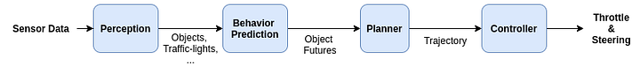
26 |
27 | * **Perception**
28 |
29 |
30 | - Perception
31 | objects,
32 | Raw sensor (lidar, camera, etc) data (image, point cloud)-> world understanding
33 | * Object detection (traffic lights, pedestrians, road signs, walkways, parking spots, lanes, etc), traffic light state detection, etc
34 | * Localization
35 | * calculate position and orientation of the vehicle as it navigates (Visual Odometry (VO)).
36 | * Deep learning used to improve the performance of VO, and to classify objects.
37 | * Examples: PoseNet and VLocNet++, use point data to estimate the 3D position and orientation.
38 | * ....
39 | * **Behavior prediction**
40 | * predict future trajectory of agents
41 | * **Planning**: decision making and generate trajectory
42 | * **Controller**: generate control commands: accelerate, break, steer left or right
43 |
44 | * Note: latency: orders of millisecond for some tasks, and order of 10 msec's for others
45 |
46 | ## Perception
47 |
48 | * 2D Object detection:
49 | * Two-stage detectors: using Region Proposal Network (RPN) to learn RoI for potential objects + bounding box predictions (using RoI pooling): (R-CNN, Fast R-CNN, Faster R-CNN, Mask-RCNN (also does segmentation)
50 | * used to outperform until focal loss
51 | * One-stage: skip proposal generation; directly produce obj BB: YOLO, SSD, RetinaNet
52 | * computationally appealing (real time)
53 | * Transformer based:
54 | * Detection Transformer ([DETR](https://github.com/facebookresearch/detr)): End-to-End Object Detection with Transformers
55 | * uses a transformer encoder-decoder architecture, backbone CNN as the encoder and a transformer-based decoder.
56 | * input image -> CNN -> feature map -> decoder -> final object queries, corresponding class labels and bounding boxes.
57 | * handles varying no. of objects in an image, as it does not rely on a fixed set of object proposals.
58 | * [More](https://towardsdatascience.com/detr-end-to-end-object-detection-with-transformers-and-implementation-of-python-8f195015c94d)
59 | * TrackFormer: Multi-Object Tracking with Transformers
60 | * on top of DETR
61 | * NMS:
62 |
63 | * 3D Object detection:
64 | * from point cloud data, ideas transferred from 2D detection
65 | * Examples:
66 | * 3D convolutions on voxelized point cloud
67 | * 2D convolutions on BEV
68 | * heavy computation
69 |
70 | * Object tracking:
71 | * use probabilistic methods such as EKF
72 | * use ML based models
73 | * use/fine-tune pre-trained CNNs for feature extraction -> do tracking with correlation or regression.
74 | * use DL based tracking algorithm, such as SORT (Simple Online and Realtime Tracking) or DeepSORT
75 |
76 |
77 | * Semantic segmentation
78 | * pixel-wise classification of image (each pixel assigned a class)
79 | * Instance segmentation
80 | * combine obj detection + semantic segmatation -> classify pixels of each instance of an object
81 |
82 |
83 | ## Behavior prediction
84 |
85 | * Main task: Motion forecasting/ trajectory prediction (future):
86 | * predict where each object will be in the future given multiple past frames
87 | * Examples:
88 | * use RNN/LSTM for prediction
89 |
90 | * Input from perception + HDMap
91 | * Options:
92 | * top-view representation: input -> CNN -> ..
93 | * vectorized: context map
94 | * graph representation: GNN
95 |
96 | * Render a bird eye view image on a single RGB image
97 | * one option for history: also render on single image
98 | * another option: use feature extractor (CNN) for each frame then use LSTM to get temporal info
99 | * Input: BEV image + (v, a, a_v)
100 | * Out: (x, y, std)
101 | 
102 | * also possible to use LSTM networks to generate waypoints in the trajectory sequentially.
103 |
104 | * Challenge: Multimodality (distribution of different modes) - future uncertain
105 |
106 |
110 |
111 |
112 | ## Planning
113 |
114 | - Decision making and generate trajectory
115 | - input: route (from A to B), context map, prediction for nearby agents
116 |
117 | - proposal: what are possible options for the plan (mathematical methods vs imitation learning) - predict what is optimal
118 |
119 | * Hierarchical RL can be used
120 | * high level planner: yield, stop, turn left/right, lane following, etc)
121 | * low level planner: execute commands
122 |
123 | - motion validation: check e.g. collision, red light, etc -> reject + ranking
124 |
125 |
126 |
127 | ## Multi task approaches
128 |
129 | * ### Perception + Behavior prediction
130 | * Fast& Furious (Uber):
131 | * Tasks: Detection, tracking, short term (e.g. 1 sec) motion forecasting
132 | * create BEV from point cloud data:
133 | * quantize 3D → 3D voxel grid (binary for occupation) → height>channel(3rd dimension) in RGB + time as 4th dimension → Single stage detector similar to SSD
134 | * deal with temporal dimension in two ways:
135 | * early fusion (aggregate temporal info at the very first layer)
136 | * late fusion (gradually merge the temporal info: allows the model to capture high-level motion features.)
137 | * use multiple predefined boxes for each feature map location (similar to SSD)
138 | * two branches after the feature map:
139 | * binary classification (P (being a vehicle) for each pre-allocated box)
140 | * predict (regress) the BB over the current frame as well as n − 1 frames into the future → size and heading
141 | 
142 | * IntentNet: learning to predict intent from raw sensor data (Uber)
143 | * Fuse BEV generated from the point cloud + HDMap info to do detection, intention prediction, and trajectory prediction.
144 | * I: Voxelized LiDAR in BEV, Rasterized HDMap
145 | * O: detected objects, trajectory, 8-class intention (keep lane, turn left, etc)
146 | ![]()
147 | 
148 |
149 | * ### Behavior Prediction + Planning (Mid-to-Mid Model)
150 |
151 | * ChauffeurNet (Waymo)
152 | * prediction and planning using single NN using Imitation Learning (IL)
153 | * More info [here](https://medium.com/aiguys/behavior-prediction-and-decision-making-in-self-driving-cars-using-deep-learning-784761ed34af)
154 |
155 | * ### End to end
156 |
157 | * Learning to drive in a day (wayve.ai)
158 | * RL to train a driving policy to follow a lane from scratch in less than 20 minutes!
159 | * Without any HDMap and hand-written rules!
160 | * Learning to Drive Like a Human
161 | * Imitation learning + RL
162 | * used some auxiliary tasks like segmentation, depth estimation, and optical flow estimation to learn a better representation of the scene and use it to train the policy.
163 |
164 | ---
165 |
166 | # Example
167 | Design an ML system to detect if a pedestrian is going to do jaywalking.
168 |
169 |
170 | ### 1. Problem Formulation
171 |
172 | - Jaywalking: a pedestrian crossing a street where there is no crosswalk or intersection.
173 | - Goal: develop an ML system that can accurately predict if a pedestrian is going to do jaywalking over a short time horizon (e.g. 1 sec) in real-time.
174 |
175 | - Pedestrian action prediction is harder than vehicle: future behavior depends on other factors such as body pose, activity, etc.
176 |
177 | * ML Objective
178 | * binary classification (predict if a pedestrian is going to do jaywalking or not in the next T seconds.)
179 |
180 | * Discuss data sources and availability.
181 |
182 | ### 2. Metrics
183 | #### Component level metrics
184 | * Object detection
185 | * Precision
186 | * calculated based on IOU threshold
187 | * AP: avg. across various IOU thresholds
188 | * mAP: mean of AP over C classes
189 | * jaywalking detection:
190 | * Precision, Recall, F1
191 | #### End-to-end metrics
192 | * Manual intervention
193 | * Simulation Errors
194 | * historical log (scene recording) w/ expert driver
195 | * input to our system and compare the decisions with the expert driver
196 |
197 |
198 | ### 3. Architectural Components
199 | * Visual Understanding System
200 | * Camera: Object detection (pedestrian, drivable region?) + tracking
201 | * [Optional] Camera + object detection: Activity recognition
202 | * Radar: 3D Object detection (skip)
203 | * Behavior prediction system
204 | * Trajectory estimation
205 | * require motion history
206 | * Ml based approach (classification)
207 | * Input:
208 | * Vision: local context: seq. of ped's cropped image (last k frames) + global context (semantically segmented images over last k frames)
209 | * Non-vision: Ped's trajectory (as BBs, last k frames) + context map + context(location, age group, etc)
210 |
211 | ### 4. Data Collection and Preparation
212 |
213 |
214 | * Data collection and annotation:
215 | * Collect datasets of pedestrian behavior, including both jaywalking and non-jaywalking behavior. This data can be obtained through public video footage or by recording video footage ourselves.
216 | * Collect a diverse dataset of video clips or image sequences from various locations, including urban and suburban areas, with different pedestrian behaviors, traffic conditions, and lighting conditions.
217 | * Annotate the data by marking pedestrians, their positions, and whether they are jaywalking or not. This can be done by drawing bounding boxes around pedestrians and labeling them accordingly (initially human labelers eventually auto-labeler system)
218 | * Targeted data collection:
219 | * in later iterations, we check cases where driver had to intervene when pedestrian jaywalking, check performance on last 20 frames, and ask labelers to label those and add to the dataset (examples need to be seen)
220 |
221 | * Labeling:
222 | * each video frame annotated with BB + pose info of the ped + activity tags (walking, standing, crossing, looking, etc) + attributes of pedestrian (age, gender, location, ets),
223 | * each video is annotated weather conditions and time of day.
224 |
225 | * Data preprocessing:
226 | * Split the dataset into training, validation, and test sets.
227 | * Normalize and resize the images to maintain consistency in input data.
228 | * Apply data augmentation techniques (e.g., rotation, flipping, brightness adjustments) to increase the dataset's size and improve model generalization.
229 | * enhance or augment the data with GANs
230 |
231 | * Data augmentation
232 |
233 |
234 |
235 | ### 5. Feature Engineering
236 |
237 | * relevant features from the video footage, such as the pedestrian's position, speed, and direction of movement.
238 | * We can also use computer vision techniques to extract features like the presence of a crosswalk, traffic lights, or other relevant environmental cues.
239 |
240 | * features from frames: fc6 features by Faster R-CNN object detector at each BB (4096T vector)
241 | * assume: we can query cropped images of last T (e.g. 5) frames of detected pedestrians from built-in object detector and tracking system
242 | * features from cropped frames: activity recognition
243 | * context map : traffic signs, street width, etc
244 | * ped's history (seq. of BB info) + current info (BB + pose info (openPose) + activity + local context) + global context (context map) + context(location, age group, etc) -> JW/NJW classifier
245 | * other features that can be fused: ped's pose, BB, semantic segmentation maps (semantic masks for relevant objects), road geometry, surrounding people, interaction with other agents
246 |
247 |
248 | ### 6. Model Development and Offline Evaluation
249 |
250 | Model selection and architecture:
251 |
252 | Assume built-in object detector and tracker. If not,
253 | * Object detection: Use a pre-trained object detection model like Faster R-CNN, YOLO, or SSD to identify and localize pedestrians in the video frames.
254 | * Object tracking:
255 | * use EKF based method or ML based method (SORT or DeepSORT)
256 | * Activity recognition:
257 | * 3D CNN, or CNN + RNN(GRU) (chose this to fit the rest of the architecture)
258 |
259 | (Output of object detection and tracking can be converted into rasterized image for each actor -> Base CNN )
260 |
261 | * Encoders:
262 | * Visual Encoder: vision content (last k frames) -> CNN base encoders + RNN for temporal info(GRU) [Another option is to use 3D CNNs]
263 | * CNN base encoder -> another RNN for activity recognition
264 | * Non-vision encoder: for temporal content use GRU
265 |
266 | * Fusion strategies:
267 | * early fusion
268 | * late fusion
269 | * hierarchical fusion
270 |
271 | * Jaywalking clf: Design a custom clf layer to classify detected pedestrians as jaywalking or not.
272 | * Example: RF, or a FC layer
273 |
274 | * we can do ablation study for selection of the fusion architecture + visual and non-visual encoders
275 | Another example:
276 | 
277 |
278 | Model training and evaluation:
279 | a. Train model(s) using the annotated dataset,
280 | + loss functions for object detection (MSE, BCE, IoU)
281 | + jaywalking classification tasks (BCE).
282 |
283 | b. Regularly evaluate the model on the validation set to monitor performance and avoid overfitting. Adjust hyperparameters, such as learning rate and batch size, if necessary.
284 |
285 | c. Once the model converges, evaluate its performance on the test set, using relevant metrics like precision, recall, F1 score, and Intersection over Union (IoU).
286 |
287 | Transfer learning for object detection (use powerful feature detectors from pre-trained models)
288 | * for fine tuning e.g. use 500 videos each 5-10 seconds, 30fps
289 |
290 | ### 7. Prediction Service
291 | * SDV on the road: will receive real-time images -> ...
292 |
293 | * Model optimization: Optimize the model for real-time deployment by using techniques such as model pruning, quantization, and TensorRT optimization.
294 |
295 | ### 8. Online Testing and Deployment
296 |
297 | Deployment: Deploy the trained model on edge devices or servers equipped with cameras to monitor real-time video feeds (e.g. traffic camera system) and detect jaywalking instances. Integrate the system with existing traffic infrastructure, such as traffic signals and surveillance systems.
298 |
299 |
300 | ### 9. Scaling, Monitoring, and Updates
301 |
302 |
303 | Continuous improvement: Regularly update the model with new data and retrain it to improve its performance and adapt to changing pedestrian behaviors and environmental conditions.
304 |
305 |
306 | * Other points:
307 | * Occlusion detection
308 | * hallucinated agent
309 | * when visual signal is imprecise
310 | * poor lighting conditions
311 |
312 |
--------------------------------------------------------------------------------
/src/MLSD/mlsd-event-recom.md:
--------------------------------------------------------------------------------
1 |
2 | # Design an event recommendation system
3 |
4 | ## 1. Problem Formulation
5 |
6 | * Clarifying questions
7 | - Use case?
8 | - event recommendation system similar to eventbrite's.
9 | - What is the main Business objective?
10 | - Increase ticket sales
11 | - Does it need to be personalized for the user? Personalized for the user
12 | - User locations? Worldwide (multiple languages)
13 | - User’s age group:
14 | - How many users? 100 million DAU
15 | - How many events? 1M events / month
16 | - Latency requirements - 200msec?
17 | - Data access
18 | - Do we log and have access to any data? Can we build a dataset using user interactions ?
19 | - Do we have textual description of items?
20 | - Can we use location data (e.g. 3rd party API)? (events are location based)
21 | - Can users become friends on the platform? Do we wanna use friendships?
22 | - Can users invite friends?
23 | - Can users RSVP or just register?
24 | - Free or Paid? Both
25 |
26 | * ML formulation
27 | * ML Objective: Recommend most relevant (define) events to the users to maximize the number of registered events
28 | * ML category: Recommendation system (ranking approach)
29 | * rule based system
30 | * embedding based (CF and content based)
31 | * Ranking problem (LTR)
32 | * pointwise, pairwise, listwise
33 | * we choose pointwise LTR ranking formulation
34 | * I/O: In: user_id, Out: ranked list of events + relevance score
35 | * Pointwise LTR classifier I/O: I: , O: P(event register) (Binary classification)
36 |
37 | ## 2. Metrics (Offline and Online)
38 |
39 | * Offline:
40 | * precision @k, recall @ k (not consider ranking quality)
41 | * MRR, mAP, nDCG (good, focus on first element, binary relevance, non-binary relevance) -> here event register binary relevance so use mAP
42 |
43 | * Online:
44 | * CTR, conversion rate, bookmark/like rate, revenue lift
45 |
46 | ## 3. Architectural Components (MVP Logic)
47 | * We two stage (funnel) architecture for
48 | * candidate generation
49 | * rule based event filtering (e.g. location, etc)
50 | * ranking formulation (pointwise LTR) binary classifier
51 |
52 | ## 4. Data preparation
53 |
54 | * Data Sources:
55 | 1. Users (user profile, historical interactions)
56 | 2. Events
57 | 3. User friendships
58 | 4. User-event interactions
59 | 5. Context
60 |
61 |
62 | * Labeling:
63 |
64 | ## 5. Feature engineering
65 |
66 | * Note: Event based recommendation is more challenging than movie/video:
67 | * events are short lived -> not many historical interactions -> cold start (constant new item problem)
68 | * So we put more effort on feature engineering (many meaningful features)
69 |
70 | * Features:
71 | - User features
72 | - age (one hot), gender (bucketize), event history
73 |
74 | - Event features
75 | - price, No of registered,
76 | - time (event time, length, remained time)
77 | - location (city, country, accessibility)
78 | - description
79 | - host (& popularity)
80 |
81 | - User Event features
82 | - event price similarity
83 | - event description similarity
84 | - no. registered similarity
85 | - same city, state, country
86 | - distance
87 | - time similarity (event length, day, time of day)
88 |
89 | - Social features
90 | - No./ ratio of friends going
91 | - invited by friends (No)
92 | - hosted by friend (similarity)
93 |
94 | - context
95 | - location, time
96 |
97 | * Feature preprocessing
98 | - one hot (gender)
99 | - bucketize + one hot (age, distance, time)
100 |
101 | * feature processing
102 | * Batch (for static) vs Online (streaming, for dynamic) processing
103 | * efficient feature computation (e.g. for location, distance)
104 | * improve: embedding learning - for users and events
105 |
106 | ## 6. Model Development and Offline Evaluation
107 |
108 | * Model selection
109 | * Binary classification problem:
110 | * LR (nonlinear interactions)
111 | * GBDT (good for structured, not for continual learning)
112 | * NN (continual learning, expressive, nonlinear rels)
113 | * we can start with GBDT as a baseline and experiment improvements by NN (both good options)
114 | * Dataset
115 | * for each user and event pair, compute features, and label 1 if registered, 0 if not
116 | * class imbalance
117 | * resampling
118 | * use focal loss or class-balanced loss
119 |
120 | ## 7. Prediction Service
121 | * Candidate generation
122 | * event filtering (millions to hundreds)
123 | * rule based (given a user, e.g. location, type, etc filters)
124 | * Ranking
125 | * compute scores for pairs, and sort
126 |
127 | ## 8. Online Testing and Deployment
128 | Standard approaches as before.
129 |
130 | ## 9. Scaling
131 |
--------------------------------------------------------------------------------
/src/MLSD/mlsd-feature-eng.md:
--------------------------------------------------------------------------------
1 |
2 | # Feature preprocessing
3 |
4 | ## Text preprocessing
5 | normalization -> tokenization -> token to ids
6 | * normalization
7 | * tokenization
8 | * Word tokenization
9 | * Subword tokenization
10 | * Character tokenization
11 | * token to ids
12 | * lookup table
13 | * Hashing
14 |
15 |
16 | ## Text encoders:
17 | Text -> Vector (Embeddings)
18 | Two approaches:
19 | - Statistical
20 | - BoW: converts documents into word frequency vectors, ignoring word order and grammar
21 | - TF-IDF: evaluates the importance of a word (term) in a document relative to a collection of documents. It is calculated as the product of two components:
22 |
23 | - Term Frequency (TF): This component measures how frequently a term occurs in a specific document and is calculated as the ratio of the number of times a term appears in a document (denoted as "term_count") to the total number of terms in that document (denoted as "total_terms"). The formula for TF is:
24 |
25 | TF(t, d) = \frac{\text{term_count}}{\text{total_terms}}
26 |
27 | - Inverse Document Frequency (IDF): This component measures the rarity of a term across the entire collection of documents and is calculated as the logarithm of the ratio of the total number of documents in the collection (denoted as "total_documents") to the number of documents containing the term (denoted as "document_frequency"). The formula for IDF is:
28 |
29 | IDF(t) = \log\left(\frac{\text{total_documents}}{\text{document_frequency}}\right)
30 |
31 | The final TF-IDF score for a term "t" in a document "d" is obtained by multiplying the TF and IDF components:
32 | TF-IDF(t,d)=TF(t,d)×IDF(t)
33 |
34 | - ML encoders
35 | - Embedding (look up) layer: a trainable layer that converts categorical inputs, such as words or IDs, into continuous-valued vectors, allowing the network to learn meaningful representations of these inputs during training.
36 | - Word2Vec: based on shallow neural networks and consists of two main approaches: Continuous Bag of Words (CBOW) and Skip-gram.
37 |
38 | - CBOW (Continuous Bag of Words):
39 |
40 | In CBOW, the model predicts a target word based on the context words (words that surround it) within a fixed window.
41 | It learns to generate the target word by taking the average of the embeddings of the context words.
42 | CBOW is computationally efficient and works well for smaller datasets.
43 | - Skip-gram:
44 |
45 | In Skip-gram, the model predicts the context words (surrounding words) given a target word.
46 | It learns to capture the relationships between the target word and its context words.
47 | Skip-gram is particularly effective for capturing fine-grained semantic relationships and works well with large datasets.
48 |
49 | Both CBOW and Skip-gram use shallow neural networks to learn word embeddings. The resulting word vectors are dense and continuous, making them suitable for various NLP tasks, such as sentiment analysis, language modeling, and text classification.
50 |
51 | - transformer based e.g. BERT: consider context, different embeddings for same words in different context
52 |
53 |
54 | ## Video preprocessing
55 | Frame-level:
56 | Decode frames -> sample frames -> resize -> scale, normalize, color correction
57 | ### Video encoders:
58 | - Video-level
59 | - process whole video to create an embedding
60 | - 3D convolutions or Transformers used
61 | - more expensive, but captures temporal understanding
62 | - Example: ViViT (Video Vision Transformer)
63 | - Frame-level (from sampled frames and aggregate frame embeddings)
64 | - less expensive (training and serving speed, compute power)
65 | - Example: ViT (Vision Transformer)
66 | - by dividing images into non-overlapping patches and processing them through a self-attention mechanism, enabling it to analyze image content; it differs from the original Transformer, which was initially designed for sequential data, like text, and relied on 1D positional encodings.
67 |
68 |
69 |
70 |
71 |
--------------------------------------------------------------------------------
/src/MLSD/mlsd-game-recom.md:
--------------------------------------------------------------------------------
1 |
2 | # Design a game recommendation engine
3 |
4 | ## 1. Problem Formulation
5 | User-game interaction
6 |
7 | Some existing data examples:
8 | * Games data
9 |
10 | * app_id,
11 | title,
12 | date_release,
13 | win,
14 | mac,
15 | linux,
16 | rating,
17 | positive_ratio,
18 | user_reviews,
19 | price_final,
20 | price_original,
21 | discount,
22 | steam_deck,
23 |
24 | * User historic data
25 |
26 | * user_id,
27 | products,
28 | reviews,
29 |
30 |
31 | * Recommendations data
32 |
33 | * app_id,
34 | helpful,
35 | funny,
36 | date,
37 | is_recommended,
38 | hours,
39 | user_id,
40 | review_id,
41 |
42 | * Reviews
43 |
44 |
45 | * Example Open Source Data: [Steam games complete dataset](https://www.kaggle.com/datasets/trolukovich/steam-games-complete-dataset) ([CF and content based github](https://github.com/AudreyGermain/Game-Recommendation-System))
46 | * Game fatures include:
47 | Url,
48 | types
49 | name,
50 | desc_snippet,
51 | recent_reviews,
52 | all_reviews,
53 | release_date,
54 | developer,
55 | publisher,
56 | popular_tag,
57 |
58 | ### Clarifying questions
59 | - Use case? Homepage?
60 | - Does user sends a text query as well?
61 | - Business objective?
62 | - Increase user engagement (play, like, click, share), purchase?, create a better ultimate gaming experience
63 | - Similar to previously played, or personalized for the user? Personalized for the user
64 | - User locations? Worldwide (multiple languages)
65 | - User’s age group:
66 | - Do users have any favorite lists, play later, etc?
67 | - How many games? 100 million
68 | - How many users? 100 million DAU
69 | - Latency requirements - 200msec?
70 | - Data access
71 | - Do we log and have access to any data? Can we build a dataset using user interactions ?
72 | - Do we have textual description of items?
73 | - can users become friends on the platform and do we wanna take that into account?
74 | - Free or Paid?
75 |
76 |
77 |
78 |
79 | ### ML objective
80 |
81 | - Recommend most engaging (define) games
82 | * Max. No. of clicks (clickbait)
83 | * Max. No. completed games/sessions/levels (bias to shorter)
84 | * Max. total hours played ()
85 | * Max. No. of relevant items (proxy by user implicit/explicit reactions) -> more control over signals, not the above shortcomings
86 |
87 | * Define relevance: e.g. like is relevant, or playing half of it is, …
88 | * ML Objective: build dataset and model to predict the relevance score b/w user and a game
89 | * I/O: I: user_id, O: ranked list of games + relevance score
90 | * ML category: Recommendation System
91 |
92 | ## 2. Metrics (Offline and Online)
93 |
94 | * Offline:
95 | * precision @k, mAP, and diversity
96 | * Online:
97 | * CTR, # of completed, # of purchased, total play time, total purchase, user feedback
98 |
99 | ## 3. Architectural Components (MVP Logic)
100 | The main approaches used for personalized recommendation systems:
101 | * Content-based filtering: suggest items similar to those user found relevant (e.g. liked)
102 | * No need for interaction data, recommends new items to users (no item cold start)
103 | * Capture unique interests of users
104 | * New user cold start
105 | * Needs domain knowledge
106 | * CF: Using user-user (user based CF) or item-item similarities (item based CF)
107 | * Pros
108 | * No domain knowledge
109 | * Capture new areas of interest
110 | * Faster than content (no content info needed)
111 | * Cons:
112 | * Cold start problem (both user and item)
113 | * No niche interest
114 | * Hybrid
115 | * Parallel hybrid: combine(CF results, content based)
116 | * Sequential: [CF based] -> Content based
117 |
118 | What do we choose?
119 | We choose a sequential hybrid model (standard e.g. for video recommendation)
120 |
121 | We follow the three stage recommender system (funnel architecture) in order to meet latency requirements and eb able to scale the system to billions of items.
122 |
123 | ```mermaid
124 | Candidate generation --> Ranking --> Re-ranking
125 | ```
126 |
127 | In the first stage, we use a light model to retrive thousands of items from millions
128 | In the second (ranking) stage, we focus on high precision using a powerful model. This will not impact serving speed much because it's only run on smaller subset of items.
129 |
130 | Candidate generation in practice comes from aggregation of different candidate generation models. Here we can assume three candidate generation modules:
131 |
132 | 1. Candidate generation 1 (Relevance based)
133 | 2. Candidate generation 2 (Popularity)
134 | 3. Candidate generation 3 (Trending)
135 |
136 | where we use CF for candidate generation 1
137 |
138 | We use content based modeling for ranking.
139 |
140 | ## 4. Data preparation
141 |
142 | Data Sources:
143 |
144 | 1. Users (user profile, historical interactions):
145 | * User profile
146 | * User_id, username, age, gender, location (city, country), lang, timezone
147 |
148 |
149 | 2. Games (structures, metadata, game content - what is it?)
150 | - Game_id, title, date, rating, expected_length?, #reviews, language, tags, description, price, developer, publisher, level, #levels
151 |
152 | 3. User-Game interactions:
153 | Historical interactions: Play, purchase, like, and search history, etc
154 | - User_id, game_id, timestamp, interaction_type(purchase, play, like, impression, search), interaction_val, location
155 |
156 |
157 | 1. Context: time of the day, day of the week, device, OS
158 |
159 | Type
160 |
161 | - Removing duplicates
162 | - filling missing values
163 | - normalizing data.
164 |
165 | ### Labeling:
166 | For features in the form of pairs -> labeling strategy based on explicit or implicit feedback
167 | e.g. "positive" if user liked the item explicitly or interacted (e.g. watched/played) at least for X (e.g. half of it).
168 | negative samples: sample from background distribution -> correct via importance smapling
169 |
170 | ## 5. Feature engineering
171 |
172 | There are several machine learning features that can be extracted from games. Here are some examples:
173 |
174 | - Game metadata features
175 | - Game state: e.g. the positions of players, the status of objects and obstacles, the time remaining, and the score.
176 | - Game mechanics: The rules and interactions that govern the game.
177 | - User engagement: e.g. the length of play sessions, frequency of play, and player retention rates.
178 | - Social interactions: b/w players: to identify patterns of behavior, such as the formation of alliances, the sharing of resources, and the types of communication used between players.
179 | - Player preferences: which game features are most popular among players, which can help inform game design decisions.
180 | - Player behaviors: player movement patterns, the types of actions taken by players, and the strategies used to achieve objectives.
181 |
182 |
183 | We select some important features as follows:
184 |
185 | * Game metadata features:
186 | * Game ID,
187 | Duration,
188 | Language,
189 | Title,
190 | Description,
191 | Genre/Category,
192 | Tags,
193 | Publisher(popularity, reviews),
194 | Release date,
195 | Ratings,
196 | Reviews,
197 | (Game content ?)
198 | game titles, genres, platforms, release dates, user ratings, and user reviews.
199 |
200 |
201 |
202 | * User profile:
203 | * User ID, Age, Gender, Language, City, Country
204 |
205 | * User-item historical features:
206 | * User-item interactions
207 | * Played, liked, impressions
208 | * purchase history (avg. price)
209 | * User search history
210 |
211 | * Context
212 |
213 |
214 | ### Feature representation:
215 |
216 | * Categorical data (game_id, user_id, language, city): Use embedding layers, learned during
217 | training
218 | * Categorical_data(gender, age): one_hot
219 | * Continuous variables: normalize, or bucketize and one-hot (e.g. price)
220 | * Text:(title, desc, tags): title/description use embeddings, pre-trained BERT, fine tune on game language?, tags: CBOW
221 | *
222 | * Game content embeddings?
223 |
224 | ## 6. Model Development and Offline Evaluation
225 |
226 | ### 6.1 Candidate Generation
227 |
228 | For candidate generation 1 (Relevance Based), we choose CF.
229 |
230 | For CF there are two embedding based modeling options:
231 | 1. Matrix Factorization
232 | * Pros: Training speed (only two matrices to learn), Serving speed (static learned embeddings)
233 | * Cons: only relies on user-item interactions (No user profile info e.g. language is used); new-user cold start problem
234 | 2. Two tower neural network:
235 | * Pros: Accepts user features (user profile + user search history) -> better quality recommendation; handles new users
236 | * Cons: Expensive training, serving speed
237 |
238 | We chose two-tower network here.
239 |
240 | #### Two-tower network
241 | * two encoder towers (user tower + encoder tower)
242 | * user tower encodes user features into user embeddings $u$
243 | * item tower encodes item features into item embeddings $v_i$
244 | * similarity $u$, $v_i$ is considered as a relevance score (ranking as classification problem)
245 |
246 |
247 | #### Loss function:
248 | Minimize cross entropy for each positive label and sampled negative examples
249 |
250 | ### 6.2 Ranking
251 | For Ranking stage, we prioritize precision over efficiency. We choose content based filtering. Choose a model that relies in item features.
252 | ML Obj options:
253 | - max P(watch| U, C)
254 | - max expected total watch time
255 | - multi-objective (multi-task learning: add corresponding losses)
256 |
257 | Model Options:
258 | - FF NN (e.g. similar tower network to a tower network) + logistic regression
259 | - Deep Cross Network (DCN)
260 |
261 | Features
262 |
263 | * Video ID embeddings (watched video embedding avg, impression video embedding),
264 | * Video historic
265 | * No. of previous impressions, reviews, likes, etc
266 | * Time features (e.g. time since last play),
267 | * Language embedding (user, item),
268 | * User profile
269 | * User Historic (e.g. search history)
270 |
271 |
272 |
273 | ### 6.3 Re-Ranking
274 | Re-ranks items by additional business criteria (filter, promote)
275 | We can use ML models for clickbait, harmful content, etc or use heuristics
276 | Examples:
277 | * Age restriction filter
278 | * Region restriction filter
279 | * Video freshness (promote fresh content)
280 | * Deduplication
281 | * Fairness, bias, etc
282 |
283 |
284 |
285 |
286 | ## 7. Prediction Service
287 | two-tower network inference: find the k-top most relevant items given a user ->
288 | It's a classic nearest neighbor problem -> use approximate nearest neighbor (ANN) algorithms
289 |
290 | ## 8. Online Testing and Deployment
291 | Standard approaches as before.
292 | ## 9. Scaling
293 | The three stage candidate generation - ranking - re-ranking can be scaled well as described earlier. It also meets the requirements of speed (funnel architecture), precision(ranking component), and diversity (multiple candid generation).
294 |
295 | ### Cold start problem:
296 | * new users: two tower architectures accepts new users and we can still use user profile info even with no interaction
297 | * new items: recommend to random users and collect some data - then fine tune the model using new data
298 |
299 | ### Training:
300 | We need to be able to fine tune the model
301 | ### Exploration exploitation trade-off
302 | - Multi-armed bandit (an agent repeatedly selects an option and receives a reward/cost. The goal of to maximize its cumulative reward over time, while simultaneously learning which options are most valuable.)
303 | ### Other Extensions:
304 | * [Multi-task learning](https://daiwk.github.io/assets/youtube-multitask.pdf)
305 | * Includes a shared feature extractor that is trained jointly with multiple prediction heads, each of which is responsible for predicting a different aspect of user behavior, such as click-through rate, watch time, and view count. The model is trained using a combination of supervised and unsupervised learning techniques, including cross-entropy loss, pairwise ranking loss, and self-supervised contrastive learning.
306 | * Positional bias (detection and correction)
307 | * Selection bias (detection and correction)
308 | * Add negative feedback (dislike)
309 | * Locality preservation:
310 | * Use sequential user behavior info (CBOW model)
311 | * effect of seasonality
312 | * what if we only have a query and personal (item, provider) history?
313 | * item embeddings, provider embeddings, query embeddings
314 | * we can build a query-aware attention mechanism that computes
315 |
316 | ### More resources
317 |
318 | * [Content-based](https://www.kaggle.com/code/fetenbasak/content-based-recommendation-game-recommender), [NLP analysis](https://www.kaggle.com/code/greentearus/steam-reviews-nlp-analysis), [Collaborative Denoising AE](https://www.kaggle.com/code/krsnewwave/collaborative-denoising-autoencoder-steam)
319 | * [User-based CF, item-based CF and MF](https://github.com/manandesai/game-recommendation-engine) ([github](https://github.com/manandesai/game-recommendation-engine/blob/main/recommenders.ipynb))
320 | * [CF and content based](https://github.com/AudreyGermain/Game-Recommendation-System)
321 |
--------------------------------------------------------------------------------
/src/MLSD/mlsd-harmful-content.md:
--------------------------------------------------------------------------------
1 | # Harmful content detection on social media
2 |
3 | ### 1. Problem Formulation
4 | * Clarifying questions
5 | * What types of harmful content are we aiming to detect? (e.g., hate speech, explicit images, cyberbullying)?
6 | * What are the potential sources of harmful content? (e.g., social media, user-generated content platforms)
7 | * Are there specific legal or ethical considerations for content moderation
8 | * What is the expected volume of content to be analyzed daily?
9 | * What are supported languages?
10 | * Are there human annotators available for labeling?
11 | * Is there a feature for users to report harmful content? (click, text, etc).
12 | * Is explainablity important here?
13 |
14 | * Integrity deals with:
15 | * Harmful content (focus here)
16 | * Harmful act/actors
17 | * Goal: monitor posts, detect harmful content, and demote/remove
18 | * Examples harmful content categories: violence, nudity, hate speech
19 | * ML objective: predict if a post is harmful
20 | * Input: Post (MM: text, image, video)
21 | * Output: P(harmful) or P(violent), P(nude), P(hate), etc
22 | * ML Category: Multimodal (Multi-label) classification
23 | * Data: 500M posts / day (about 10K annotated)
24 | * Latency: can vary for different categories
25 | * Able to explain the reason to the users (category)
26 | * support different languages? Yes
27 |
28 | ### 2. Metrics
29 | - Offline
30 | - F1 score, PR-AUC, ROC-AUC
31 | - Online
32 | - prevalence (percentage of harmful posts didn't prevent over all posts), harmful impressions, percentage of valid (reversed) appeals, proactive rate (ratio of system detected over system + user detected)
33 |
34 | ### 3. Architectural Components
35 | * Multimodal input (text, image, video, etc):
36 | * Multimodal fusion techniques
37 | * Early Fusion: modalities combined first, then make a single prediction
38 | * Late Fusion: process modalities independently, fuse predictions
39 | * cons: separate training data for modalities, comb of individually safe content might be harmful
40 | * Multi-Label/Multi-Task classification
41 | * Single binary classifier (P(harmful))
42 | * easy, not explainable
43 | * One binary classifier per harm category (p(violence), p(nude), p(hate))
44 | * multiple models, trained and maintained separately, expensive
45 | * Single multi-label classifier
46 | * complicated task to learn
47 | * Multi-task classifier: learn multi tasks simultanously
48 | * single shared layers (learns similarities between tasks) -> transformed features
49 | * task specific layers: classification heads
50 | * pros: single model, shared layers prevent redundancy, train data for each task can be used for others as well (limited data)
51 |
52 | ### 4. Data Collection and Preparation
53 |
54 | * Main actors for which data is available:
55 | * Users
56 | * user_id, age, gender, location, contact
57 | * Items(Posts)
58 | * post_id, author_id, text context, images, videos, links, timestamp
59 | * User-post interactions
60 | * user_id, post_id, interaction_type, value, timestamp
61 |
62 |
63 | ### 5. Feature Engineering
64 | Features:
65 | Post Content (text, image, video) + Post Interactions (text + structured) + Author info + Context
66 | * Posts
67 | * Text:
68 | * Preprocessing (normalization + tokenization)
69 | * Encoding (Vectorization):
70 | * Statistical (BoW, TF-IDF)
71 | * ML based encoders (BERT)
72 | * We chose pre-trained ML based encoders (need semantics of the text)
73 | * We chose Multilingual Distilled (smaller, faster) version of BERT (need context), DistilmBERT
74 | * Images/ Videos:
75 | * Preprocessing: decoding, resize, scaling, normalization
76 | * Feature extraction: pre-trained feature extractors
77 | * Images:
78 | * CLIP's visual encoder
79 | * SImCLR
80 | * Videos:
81 | * VideoMoCo
82 | * Post interactions:
83 | * No. of likes, comments, shares, reports (scale)
84 | * Comments (text): similar to the post text (aggregate embeddings over comments)
85 | * Users:
86 | * Only use post author's info
87 | * demographics (age, gender, location)
88 | * account features (No. of followers /following, account age)
89 | * violation history (No of violations, No of user reports, profane words rate)
90 | * Context:
91 | * Time of day, device
92 |
93 | ### 6. Model Development and Offline Evaluation
94 | * Model selection
95 | * NN: we use NN as it's commonly used for multi-task learning
96 | * HP tuniing:
97 | * No of hidden layers, neurons in layers, act. fcns, learning rate, etc
98 | * grid search commonly used
99 | * Dataset:
100 | * Natural labeling (user reports) - speed
101 | * Hand labeling (human contractors) - accuracy
102 | * we use natural labeling for train set (speed) and manual for eval set (accuracy)
103 | * loss function:
104 | * L = L1 + L2 + L3 ... for each task
105 | * each task is a binary classific so e.g. CE for each task
106 | * Challenge for MM training:
107 | * overfitting (when one modality e.g. image dominates training)
108 | * gradient blending and focal loss
109 |
110 | ### 7. Prediction Service
111 | * 3 main components:
112 | * Harmful content detection service
113 | * Demoting service (prob of harm with low confidence)
114 | * violation service (prob of harm with high confidence)
115 |
116 | ### 8. Online Testing and Deployment
117 |
118 | ### 9. Scaling, Monitoring, and Updates
119 |
120 | ### 10. Other topics
121 | * biases by human labeling
122 | * use temporal information (e.g. sequence of actions)
123 | * detect fake accounts
124 | * architecture improvement: linear transformers
125 |
--------------------------------------------------------------------------------
/src/MLSD/mlsd-image-search.md:
--------------------------------------------------------------------------------
1 | # Image Search System (Pinterest)
2 |
3 | ### 1. Problem Formulation
4 | * Clarifying questions
5 | - What is the primary (business) objective of the visual search system?
6 | - What are the specific use cases and scenarios where it will be applied?
7 | - What are the system requirements (such as response time, accuracy, scalability, and integration with existing systems or platforms)?
8 | - How will users interact with the system? (click, like, share, etc)? Click only
9 | - What types of visual content will the system search through (images, videos, etc.)? Images only
10 | - Are there any specific industries or domains where this system will be deployed (e.g., fashion, e-commerce, art, industrial inspection)?
11 | - What is the expected scale of the system in terms of data and user interactions?
12 | - Personalized? not required
13 | - Can we use metadata? In general yes, here let's not.
14 | - Can we assume the platform provides images which are safe? Yes
15 | * Use case(s) and business goal
16 | * Use case: allowing users to search for visually similar items, given a query image by the user
17 | * business goal: enhance user experience, increase click through rate, conversion rates, etc (depends on use case)
18 | * Requirements
19 | * response time, accuracy, scalability (billions of images)
20 | * Constraints
21 | * budget limitations, hardware limitations, or legal and privacy constraints
22 | * Data: sources and availability
23 | * sources of visual data: user-generated, product catalogs, or public image databases?
24 | * Available?
25 | * Assumptions
26 | * ML formulation:
27 | * ML Objective: retrieve images that are similar to query image in terms of visual content
28 | * ML I/O: I: a query image, and O: a ranked list of most similar images to the query image
29 | * ML category: Ranking problem (rank a collection of items based on their relevance to a query)
30 |
31 | ### 2. Metrics
32 | * Offline metrics
33 | * MRR
34 | * Recall@k
35 | * Precision@k
36 | * mAP
37 | * nDCG
38 | * Online metrics
39 | * CTR
40 | * Time spent on images
41 |
42 | ### 3. Architectural Components
43 | * High level architecture
44 | * Representation learning:
45 | * transform input data into representations (embeddings) - similar images are close in their embedding space
46 | * use distance between embeddings as a similarity measure between images
47 |
48 | ### 4. Data Collection and Preparation
49 | * Data Sources
50 | * User profile
51 | * Images
52 | * image file
53 | * metadata
54 | * User-image interactions: impressions, clicks:
55 | * Context
56 | * Data storage
57 | * ML Data types
58 | * Labelling
59 |
60 | ### 5. Feature Engineering
61 | * Feature selection
62 | * User profile : User_id, username, age, gender, location (city, country), lang, timezone
63 | * Image metadata: ID, user ID, tags, upload date, ...
64 | * User-image interactions: impressions, clicks:
65 | * user id, Query img id, returned img id, interaction type (click, impression), time, location
66 | * Feature representation
67 | * Representation learning (embedding)
68 | * Feature preprocessing
69 | * common feature preprocessing for images:
70 | * Resize (e.g. 224x224), Scale (0-1), normalize (mean 0, var 1), color mode (RGB, CMYK)
71 |
72 | ### 6. Model Development and Offline Evaluation
73 | * Model selection
74 | * we choose NN because of
75 | * unstructured data (images, text) -> NN good at it
76 | * embeddings needed
77 | * Architecture type:
78 | * CNN based e.g. ResNet
79 | * Transformer based (ViT)
80 | * Example: Image -> Convolutional layers -> FC layers -> embedding vector
81 | * Model Training
82 | * contrastive learning -> used for image representation learning
83 | * train to distinguish similar and dissimilar items (images)
84 | * Dataset
85 | * each data point: query img, positive sample (similar to q), n - 1 neg samples (dissimilar)
86 | * query img : randomly choose
87 | * neg samples: randomly choose
88 | * positive samples: human judge, interactions (e.g. click) as a proxy, artificial image generated from q (self supervision)
89 | * human: expensive, time consuming
90 | * interactions: noisy and sparse
91 | * artificial: augment (e.g. rotate) and use as a positive sample (similar to simCLR or MoCo) - data distribution differs in reality
92 | * Loss Function: contrastive loss
93 | * contrastive loss:
94 | * works on pairs (Eq, Ei)
95 | * calculate distance: b/w pairs -> softmax -> cross entropy <- Labels
96 | * Model eval and HP tuning
97 | * Iterations
98 |
99 | ### 7. Prediction Service
100 | * Prediction pipeline
101 |
102 | * Embedding generation service
103 | * image -> preprocess -> embedding gen (ML model) -> img embedding
104 | * NN search service
105 | * retrieve the most similar images from embedding space
106 | * Exact: O(N.D)
107 | * Approximate(ANN) - sublinear e.g. O(D.logN)
108 | * Tree based ANN (e.g. R-trees, Kd-trees)
109 | * partition space into two (or more) at each non-leaf node,
110 | * only search the partition for query q
111 | * Locality Sensitive Hashing LSH
112 | * using hash functions to group points into buckets (close points into same buckets)
113 | * Clustering based
114 | * We use ANN using an existing library like Faiss (Facebook)
115 | * Re-ranking service
116 | * business level logic and policies (e.g. filter inappropriate or private items, deduplicate, etc)
117 | * Indexing pipeline
118 | * Indexing service: indexes images by their embeddings
119 | * keep the table updated for new images
120 | * increases memory usage -> use optimization (vector / product quantization)
121 |
122 | ### 8. Online Testing and Deployment
123 | * A/B Test
124 | * Deployment and release
125 |
126 | ### 9. Scaling, Monitoring, and Updates
127 | * Scaling (SW and ML systems)
128 | * Monitoring
129 | * Updates
130 |
131 | ### 10. Other points:
132 |
133 |
--------------------------------------------------------------------------------
/src/MLSD/mlsd-metrics.md:
--------------------------------------------------------------------------------
1 | # Offline Metrics
2 |
3 | These offline metrics are commonly used in search, information retrieval, and recommendation systems to evaluate the quality of results or recommendations:
4 |
5 | ### Recall@k:
6 | - Definition: Recall@k evaluates the fraction of relevant items retrieved among the top k recommendations over total relevant items. It measures the system's ability to find all relevant items in a fixed-sized list.
7 | - Use Case: In information retrieval and recommendation systems, Recall@k is crucial when it's essential to ensure that no relevant items are missed in the top k recommendations.
8 |
9 | ### Precision@k:
10 |
11 | - Definition: Precision@k assesses the fraction of retrieved items that are relevant among the top k recommendations. It measures the system's ability to provide relevant content at the top of the list.
12 | - Use Case: Precision@k is vital when there's a need to present users with highly relevant content in the initial recommendations. It helps in reducing user frustration caused by irrelevant suggestions.
13 |
14 | ### Mean Reciprocal Rank (MRR):
15 |
16 | - Definition: MRR measures the effectiveness of a system in ranking the most relevant items at the top of a list. It calculates the average of reciprocal ranks of the first correct item found in each ranked list of results:
17 | MRR = 1/m \Sum(1/rank_i)
18 | - Use Case: MRR is often used in search and recommendation systems to assess how quickly users find relevant content. It's particularly useful when there is only one correct answer or when the order of results matters.
19 |
20 | ### Mean Average Precision (mAP):
21 |
22 | - Definition: mAP computes the average precision across multiple queries or users. Precision is calculated for each query, and the mean of these precisions is taken to provide a single performance score.
23 | - Use Case: mAP is valuable in scenarios where there are multiple users or queries, and you want to assess the overall quality of recommendations or search results across a diverse set of queries. mAP works well for binary relevances. For continues scores, we use nDCG.
24 |
25 | ### Discounted Cumulative Gain (DCG):
26 | - Definition: Discounted Cumulative Gain (DCG) is a widely used evaluation metric primarily applied in the fields of information retrieval, search engines, and recommendation systems.
27 | - DCG quantifies the quality of a ranked list of items or search results by considering two key aspects:
28 | 1. Relevance: Each item in the list is associated with a relevance score, which indicates how relevant it is to the user's query or preferences. Relevance scores are typically on a scale, with higher values indicating greater relevance.
29 | 2. Position: DCG takes into account the position of each item in the ranked list. Items appearing higher in the list are considered more important because users are more likely to interact with or click on items at the top of the list.
30 | - DCG calculates the cumulative gain by summing the relevance scores of items in the ranked list up to a specified position.
31 | - To reflect the decreasing importance of items further down the list, DCG applies a discount factor, often logarithmic in nature.
32 | - Use case:
33 | - DCG is employed to evaluate how effectively a system ranks and presents relevant items to users.
34 | - It is instrumental in optimizing search and recommendation algorithms, ensuring that highly relevant items are positioned at the top of the list for user engagement and satisfaction.
35 |
36 | ### Normalized Discounted Cumulative Gain (nDCG):
37 |
38 | - Definition: nDCG measures the quality of a ranked list by considering the graded relevance of items. It discounts the relevance of items as they appear further down the list and normalizes the score. It is calculated as the fraction of DCG over the Ideal DCG(IDCG) for an ideal ranking.
39 | - Use Case: nDCG is beneficial when relevance is not binary (i.e., there are degrees of relevance), and you want to account for the diminishing importance of items lower in the ranking.
40 |
41 | # Cross Entropy and Normalized Cross Entropy
42 | - The CE (also a loss function), measures how well the predicted probabilities align with the true class labels. It's defined as:
43 |
44 | - For binary classification:
45 | CE = - [y * log(p) + (1 - y) * log(1 - p)]
46 |
47 | - For multi-class classification:
48 | CE = - Σ(y_i * log(p_i))
49 |
50 | Where:
51 | - y is the true class label (0 or 1 for binary, one-hot encoded vector for multi-class).
52 | - p is the predicted probability assigned to the true class label.
53 | - The negative sign ensures that the loss is minimized when the predicted probabilities match the true labels. (the lower the better)
54 | - NCE: CE(ML model) / CE(simple baseline)
55 |
56 | ### Ranking:
57 | * Precision @k and Recall @k not a good fit (not consider ranking quality of out)
58 | * MRR, mAP, and nDCG good:
59 | * MRR: focus on rank of 1st relevant item
60 | * nDCG: relevance b/w user and item is non-binary
61 | * mAP: relevance is binary
62 | * Ads ranking: NCE
63 |
64 | # Online metrics
65 | * CTR
66 |
67 |
68 | - Definition:
69 |
70 | - Click-Through Rate (CTR) is a metric that quantifies user engagement with a specific item or element, such as an advertisement, a search result, a recommended product, or a link.
71 | - It is calculated by dividing the number of clicks on the item by the total number of impressions (or views) it received.
72 | - Formula for CTR:
73 | CTR= Number of Clicks/Number of Impressions ×100%
74 |
75 | - Impressions: Impressions refer to the total number of times the item was displayed or viewed by users. For ads, it's the number of times the ad was shown to users. For recommendations, it's the number of times an item was recommended to users.
76 |
77 | - Use Cases:
78 | - Online Advertising campaigns: widely used to assess how well ads are performing. A high CTR indicates that the ad is compelling and relevant to the target audience.
79 | - Recommendation Systems: CTR is used to measure how effectively recommended items attract user clicks.
80 | - Search Engines: CTR is used to evaluate the quality of search results. High CTR for a search result indicates that it was relevant to the user's query.
81 |
82 | * Conversion Rate: Conversion Rate measures the percentage of users who take a specific desired action after interacting with an item, such as making a purchase, signing up for a newsletter, or filling out a form. It helps assess the effectiveness of a call to action.
83 |
84 | * Bounce Rate: Bounce Rate calculates the percentage of users who visit a webpage or view an item but leave without taking any further action, such as navigating to another page or interacting with additional content. A high bounce rate may indicate that users are not finding the content engaging.
85 |
86 | * Engagement Rate: Engagement Rate evaluates the level of user interaction and participation with content or ads. It can include metrics like comments, shares, likes, or time spent on a webpage. A high engagement rate suggests that users are actively involved with the content.
87 |
88 | * Time on Page: Time on Page measures how long users spend on a webpage or interacting with a specific piece of content. It helps evaluate user engagement and the effectiveness of content in holding user attention.
89 |
90 | * Return on Investment (ROI): ROI assesses the financial performance of an advertising or marketing campaign by comparing the costs of the campaign to the revenue generated from it. It's crucial for measuring the profitability of marketing efforts.
--------------------------------------------------------------------------------
/src/MLSD/mlsd-mm-video-search.md:
--------------------------------------------------------------------------------
1 | # Multimodal Video Search System
2 |
3 | ### 1. Problem Formulation
4 | * Clarifying questions
5 | - What is the primary (business) objective of the search system?
6 | - What are the specific use cases and scenarios where it will be applied?
7 | - What are the system requirements (such as response time, accuracy, scalability, and integration with existing systems or platforms)?
8 | - What is the expected scale of the system in terms of data and user interactions?
9 | - Is their any data available? What format?
10 | - Can we use video metadata? Yes
11 | - Personalized? not required
12 | - How many languages needs to be supported?
13 |
14 | * Use case(s) and business goal
15 | * Use case: user enters text query into search box, system shows the most relevant videos
16 | * business goal: increase click through rate, watch time, etc.
17 | * Requirements
18 | * response time, accuracy, scalability (50M DAU)
19 | * Constraints
20 | * budget limitations, hardware limitations, or legal and privacy constraints
21 | * Data: sources and availability
22 | * Sources: videos (1B), text
23 | * 10M pairs of . Videos have metadata (title, description, tags) in text format
24 | * Assumptions
25 | * ML formulation:
26 | * ML Objective: retrieve videos that are relevant to a text query
27 | * ML I/O: I: text query from a user, O: ranked list of relevant videos on a video sharing platform
28 | * ML category: Visual search + Text Search systems
29 |
30 |
31 | ### 2. Metrics
32 | - Offline
33 | - Precision@k, mAP, Recall@k, MRR
34 | - we choose MRR (avg rank of first relevant element in results) due to the format of our eval data pair
35 | - Online
36 | - CTR: problem: doesn't track relevancy, click baits
37 | - video completion rate: partially watched videos might still found relevant by user
38 | - total watch time
39 | - we choose total watch time: good indicator of relevance
40 |
41 | ### 3. Architectural Components
42 | Multimodal search (video, text) for video content from text query:
43 | - Visual search system
44 | - Text query -> videos (based on similarity of text and visual content)
45 | - Two tower embedding architecture (video and text_query encoders)
46 | - Textual search system
47 | - search for most similar titles, descs, and tags w/ text query
48 | - we can use Inverted Index (e.g. elastic search) for efficient full text search
49 | - An inverted index is a data structure that maps terms (words) to the documents or locations where they appear, enabling efficient text-based document retrieval, commonly used in search engines.
50 |
51 | ### 4. Data Collection and Preparation
52 | We use provided annotated data in the format of .
53 | ### 5. Feature Engineering
54 | - Preprocessing unstructured data
55 | - Text pre-processing : normalization, tokenization, token to ids
56 | - Video preprocessing: decode into frames -> sample -> resize -> scale, normalize, color correct
57 |
58 | ### 6. Model Development and Offline Evaluation
59 | * Model Selection
60 | - Text encoders:
61 | - Text -> Vector (Embeddings)
62 | - Two approaches:
63 | - Statistical (BoW, TF-IDF)
64 | - ML encoders (word2vec, transformer based e.g. BERT)
65 | - We chose transformer based (BERT).
66 |
67 | - Video encoders:
68 | - Video-level
69 | - more expensive, but captures temporal understanding
70 | - Example: ViViT (Video Vision Transformer)
71 | - Frame-level (from sample frames and aggregate)
72 | - less expensive (training and serving speed, compute power)
73 | - Example: ViT
74 |
75 |
76 | * Model Training
77 | - contrastive learning (similar to visual search system).
78 |
79 | ### 7. Prediction Service
80 | Components:
81 | - Visual search from text query
82 | - text -> preprocess -> encoder -> embedding
83 | - videos are indexed by their encoded embeddings
84 | - search: using approximate nearest neighbor search (ANN)
85 | - Textual search
86 | - using Elasticsearch (full text / fuzzy search)
87 | - Fusion
88 | - re-rank based on weighted sum of rel scores
89 | - re-rank using a model
90 | - Re-ranking
91 | - business level logic and policies
92 |
93 | ### 8. Online Testing and Deployment
94 |
95 | ### 9. Scaling, Monitoring, and Updates
96 |
--------------------------------------------------------------------------------
/src/MLSD/mlsd-modeling-popular-archs.md:
--------------------------------------------------------------------------------
1 |
2 | # Popular Neural Network Architectures
3 |
4 | * ## Two stage funnel architecture
5 | * candidate generation + ranking
6 |
7 | * ## Two-tower architecture
8 |
9 | * ## Wide and deep learning
10 |
11 | * ## Deep cross network
12 |
13 | * ## Multi-task learning
14 |
15 | * ## Transformers
16 |
17 | * ## Encoder, Decoder, Encoder-decoder
18 |
19 | * ## Knowledge Distillation (student-teacher network)
20 |
21 | * ## Contrastive Learning
22 |
23 | * ## NLP
24 |
25 | * BERT, T5, GPT
26 |
27 | * ## Computer Vision
28 |
29 | * Object detectors (single stage, two-stage)
30 | * Vision Transformer
31 |
--------------------------------------------------------------------------------
/src/MLSD/mlsd-newsfeed.md:
--------------------------------------------------------------------------------
1 | # News Feed System
2 |
3 | ### 1. Problem Formulation
4 | show feed (recent posts and activities from other users) on a social network platform
5 | * Clarifying questions
6 | * What is the primary business objective of the system? (increase user engagement)
7 | * Do we show only posts or also activities from other users?
8 | * What types of engagement are available? (like, click, share, comment, hide, etc)? Which ones are we optimizing for?
9 | * Do we display ads as well?
10 | * What types of data do the posts include? (text, image, video)?
11 | * Are there specific user segments or contexts we should consider (e.g., user demographics)?
12 | * Do we have negative feedback features (such as hide ad, block, etc)?
13 | * What type of user-ad interaction data do we have access to can we use it for training our models?
14 | * Do we need continual training?
15 | * How do we collect negative samples? (not clicked, negative feedback).
16 | * How fast the system needs to be?
17 | * What is the scale of the system?
18 | * Is personalization needed? Yes
19 |
20 | * Use case(s) and business goal
21 | * use case: show friends most engaging (and unseen) posts and activities on a social network platform app (personalized to user)
22 | * business objective: Maximize user engagement (as a set of interactions)
23 |
24 | * Requirements;
25 | * Latency: 200 msec of newsfeed refreshed results after user opens/refreshes the app
26 | * Scalability: 5 B total users, 2 B DAU, refresh app twice
27 |
28 | * Constraints:
29 | * Privacy and compliance with data protection regulations.
30 |
31 | * Data: Sources and Availability:
32 | * Data sources include user interaction logs, ad content data, user profiles, and contextual information.
33 | * Historical click and impression data for model training and evaluation.
34 |
35 | * Assumptions:
36 | * Users' engagement behavior can be characterized by their explicit (e.g. like, click, share, comment, etc) or implicit interactions (e.g. dwell time)
37 |
38 | * ML Formulation:
39 | * Objective:
40 | * maximize number of explicit, implicit, or both type of reactions (weighted)
41 | * implicit: more data, explicit: stronger signal, but less data -> weighted score of different interactions: share > comment > like > click etc
42 | * I/O: I: user_id, O: ranked list of unseen posts sorted by engagement score (wighted sum)
43 | * Category: Ranking problem: can be solved as pointwise LTR with multi/label (multi-task) classification
44 |
45 | ### 2. Metrics
46 | * Offline
47 | * ROC AUC (trade-off b/w TPR and FPR)
48 | * Online
49 | * CTR,
50 | * Reactions rate (like rate, comment rate, etc)
51 | * Time spent
52 | * User satisfaction (survey)
53 |
54 | ### 3. Architectural Components
55 | * High level architecture
56 | * We can use point-wise learning to rank (LTR) formulation
57 | * Options for multi-label/task classification:
58 | * Use N independent classifiers (expensive to train and maintain)
59 | * Use a multi-task classifier
60 | * learn multi tasks simultaneously
61 | * single shared layers (learns similarities between tasks) -> transformed features
62 | * task specific layers: classification heads
63 | * pros: single model, shared layers prevent redundancy, train data for each task can be used for others as well (limited data)
64 |
65 | ### 4. Data Collection and Preparation
66 | * Data Sources
67 | * Users,
68 | * Posts,
69 | * User-post interaction
70 | * User-user (friendship)
71 |
72 | * Labelling
73 |
74 | ### 5. Feature Engineering
75 |
76 | * Feature selection
77 | * Posts:
78 | * Text
79 | * Image/videos
80 | * No of reactions (likes, shares, replies, etc)
81 | * Age
82 | * Hashtags
83 | * User:
84 | * ID, username
85 | * Demographics (Age, gender, location)
86 | * Context (device, time of day, etc)
87 | * Interaction history (e.g. user click rate, total clicks, likes, et )
88 | * User-Post interaction:
89 | * IDs(user, Ad), interaction type, time, location
90 | * User-user(post author) affinities
91 | * connection type
92 | * reaction history (No liked/commented/etc posts from author)
93 |
94 | * Feature representation / preparation
95 | * Text:
96 | * use a pre-trained LM to get embeddings
97 | * use BERT here (posts are in phrases usually, context aware helps)
98 |
99 | * Image / Video:
100 | * preprocess
101 | * use pre-trained models e.g. SimCLR / CLIP to convert -> feature vector
102 |
103 | * Dense numerical features:
104 | * Engagement feats (No of clicks, etc)
105 | * use directly + scale the range
106 | * Discrete numerical:
107 | * Age: bucketize into categorical then one hot
108 | * Hashtags:
109 | * tokenize, token to ID, simple vectorization (TF-IDF or word2vec) - no context
110 |
111 |
112 | ### 6. Model Development and Offline Evaluation
113 |
114 | * Model selection
115 | * We choose NN
116 | * unstructured data (text, img, video)
117 | * embedding layers for categorical features
118 | * fine tune pre-trained models used for feat eng.
119 | * multi-labels
120 | * P(click), P(like), P(Share), P(comment)
121 | * Two options:
122 | * N NN classifiers
123 | * Multi task NN (choose this)
124 | * Shared layers
125 | * Classification heads (click, like, share, comment)
126 | * Passive users problem:
127 | * All their Ps will be small
128 | * add two more heads
129 | * Dwell time (seconds spent on post)
130 | * P(skip) (skip = spend time < t)
131 |
132 |
133 | * Model Training
134 | * Loss function:
135 | * L = sum of L_is for each task
136 | * for binary classif tasks: CE
137 | * for regression task: MAE, MSE, or Huber loss
138 | * Dataset
139 | * use features, post features, interactions, labels
140 | * labels: positive, negative for each task (like, didn't like etc)
141 | * for dwell time: it's a regression
142 | * Imbalanced dataset: downsample negative
143 | * Model eval and HP tuning
144 | * Iterations
145 |
146 | ### 7. Prediction Service
147 | * Data Prep pipeline
148 | * static features -> batch feature compute (daily, weekly) -> feature store
149 | * dynamic features: # of post clicks, etc _> streaming
150 |
151 | * Prediction pipeline
152 | * two stage (funnel) architecture
153 | * candidate generation / retrieval service
154 | * rule based
155 | * filter and fetch unseen posts by users under certain criteria
156 | * Ranking
157 | * features -> model -> engagement prob. -> sort
158 | * re-ranking: business logic, additional logic and filters (e.g. user interest category)
159 | * Continual learning pipeline
160 | * fine tune on new data, eval, and deploy if improves metrics
161 |
162 | ### 8. Online Testing and Deployment
163 | * A/B Test
164 | * Deployment and release
165 |
166 | ### 9. Scaling, Monitoring, and Updates
167 | * Scaling (SW and ML systems)
168 | * Monitoring
169 | * Updates
170 |
171 | ### 10. Other topics
172 | * Viral posts / Celebrities posts
173 | * New users (cold start)
174 | * Positional data bias
175 | * Update frequency
176 | * calibration:
177 | * fine-tuning predicted probabilities to align them with actual click probabilities
178 | * data leakage:
179 | * info from the test or eval dataset influences the training process
180 | * target leakage, data contamination (from test to train set)
181 | * catastrophic forgetting
182 | * model trained on new data loses its ability to perform well on previously learned tasks
183 |
--------------------------------------------------------------------------------
/src/MLSD/mlsd-prediction.md:
--------------------------------------------------------------------------------
1 | # Prediction Service
2 |
3 | ## Embedding Generation
4 |
5 | ## Indexing Service
6 |
7 | - Index text, image, video by their embeddings
8 | - provides and keeps updating a look up table
9 | - index new items upon arrival
10 | - pros: efficient search by NN service
11 | - cons: memory usage
12 | - optimization techniques
13 |
14 |
15 | ## Nearest Neighbor Service
16 |
17 | - Approximate Nearest Neighbors (ANN)
18 | - Tree-based ANN
19 | - Locality-sensitive hashing (LSH)
20 | - Clustering based
--------------------------------------------------------------------------------
/src/MLSD/mlsd-preprocessing.md:
--------------------------------------------------------------------------------
1 | ## Preprocessing Text:
2 |
3 | * ### Normalization -> Tokenization [Pre-Tokenization -> Tokenizer Model -> Post-processing] -> Token to ids (lookup table, hashing)
4 | ## Preprocessing Images:
5 |
6 | ## Preprocessing Videos:
7 | Decode frames -> sample frames -> Resize -> Scale, normalize
8 |
9 |
--------------------------------------------------------------------------------
/src/MLSD/mlsd-pymk.md:
--------------------------------------------------------------------------------
1 | # Friends/Follower recommendation (People you may know)
2 |
3 | ### 1. Problem Formulation
4 | Recommend a list of users that you may want to connect with
5 | * Clarifying questions
6 | * What is the primary business objective of the system?
7 | * What's the primary use case of the system?
8 | * Are there specific factors needs to be considered for recommendations?
9 | * Are friendships/connections symmetrical?
10 | * What is the scale of the system? (users, connections)
11 | * can we assume the social graph is not very dynamic?
12 | * Do we need continual training?
13 | * How do we collect negative samples? (not clicked, negative feedback).
14 | * How fast the system needs to be?
15 | * Is personalization needed? Yes
16 |
17 | ##
18 | * Use case(s) and business goal
19 | * use case: PYMMK: recommend a list of users to connect with on social media app (e.g. facebook, linkedin)
20 | * business objective: maximize number of formed connections
21 |
22 | * Requirements;
23 | * Scalability: 1 B total users, on avg. 10000 connection per user
24 |
25 | * Constraints:
26 | * Privacy and compliance with data protection regulations.
27 |
28 | * Data: Sources and Availability:
29 |
30 | * Assumptions:
31 | * symmetric firendships
32 |
33 | * ML Formulation:
34 | * Objective:
35 | * maximize number of formed connections
36 | * I/O: I: user_id, O: ranked list of recommended users sorted by the relevance to the user
37 | * ML Category: two options:
38 | * Ranking problem:
39 | * pointwise LTR - binary classifier (user_i, user_j) -> p(connection)
40 | * cons: doesn't capture social connections
41 | * Graph representation (edge prediction)
42 | * supplement with graph info (nodes, edges)
43 | * input: social graph, predict edge b/w nodes
44 |
45 | ### 2. Metrics
46 | * Offline
47 | * GNN model: binary classification -> ROC-AUC
48 | * Recommendation system: binary relationships -> mAP
49 |
50 | * Online
51 | * No of friend requests sent over X time
52 | * No of friend requests accepted over X time
53 |
54 | ### 3. Architectural Components
55 | * High level architecture
56 | * Node-level predictions
57 | * Edge-level predictions
58 |
59 | ### 4. Data Collection and Preparation
60 | * Data Sources
61 | * Users,
62 | * demographics, edu and work backgrounds, skills, etc
63 | * note: standardized data (e.g. cs / computer science)
64 | * User-user connections,
65 | * User-user interactions,
66 |
67 | * Labelling
68 |
69 | ### 5. Feature Engineering
70 |
71 | * Feature selection
72 |
73 | * User:
74 | * ID, username
75 | * Demographics (Age, gender, location)
76 | * Account/Network info: No of connections, followers, following, requests, etc, account age
77 | * Interaction history (No of likes, shares, comments)
78 | * Context (device, time of day, etc)
79 |
80 | * User-user connections:
81 | * Connection: IDs(user1, user2), connection type, timestamp, location
82 | * edu and work affinity: major similarity, companies in common, industry similarity, etc
83 | * social affinity: No. mutual connections (time discounted)
84 | * User-user interactions:
85 | * IDs(u user1, user2), interaction type, timestamp
86 |
87 |
88 |
89 |
90 | ### 6. Model Development and Offline Evaluation
91 |
92 | * Model selection
93 | * We choose GNN
94 | * operate on graph data
95 | * predict prob of edge
96 | * input: graph (node and edge features)
97 | * output: embedding of each node
98 | * use similarities b/w node embeddings for edge prediction
99 |
100 |
101 | * Model Training
102 | * snapshot of G at t. model predict connections at t+1
103 | * Dataset
104 | * create a snapshot at time t
105 | * compute node and edge features
106 | * create labels using snapshot at t + 1 (if connection formed, positive)
107 | * Model eval and HP tuning
108 | * Iterations
109 |
110 | ### 7. Prediction Service
111 | * Prediction pipeline
112 | * Candidate generation
113 | * Friends of Friends (FoF) - rule based - from 1B to 1K.1K = 1M candidates -> FoF service
114 | * Scoring service (using GNN model -> embeddings -> similarity scores)
115 | * sort by score
116 | * pre-compute PYMK tables for each / active users and store in DB
117 | * re-rank based on business logic
118 |
119 | ### 8. Online Testing and Deployment
120 | * A/B Test
121 | * Deployment and release
122 |
123 | ### 9. Scaling, Monitoring, and Updates
124 | * Scaling (SW and ML systems)
125 | * Monitoring
126 | * Updates
127 |
128 | ### 10. Other topics
129 | * add a lightweight ranker
130 | * bias problem
131 | * delayed feedback problem (user accepts after days)
132 | * personalized random walk (for baseline)
133 |
--------------------------------------------------------------------------------
/src/MLSD/mlsd-search.md:
--------------------------------------------------------------------------------
1 | # Search System
2 |
3 | ### 1. Problem Formulation
4 | * Clarifying questions
5 | - Is it a generalized search engine (like google) or specialized (like amazon product)?
6 | - What is the primary (business) objective of the search system?
7 | - What are the specific use cases and scenarios where it will be applied?
8 | - What are the system requirements (such as response time, accuracy, scalability, and integration with existing systems or platforms)?
9 | - What is the expected scale of the system in terms of data and user interactions?
10 | - Is their any data available? What format?
11 | - Personalized? not required
12 | - How many languages needs to be supported?
13 | - What types of items (products) are available on the platform, and what attributes are associated with them?
14 | - What are the common user search behaviors and patterns? Do users frequently use filters, sort options, or advanced search features?
15 | - Are there specific search-related challenges unique to the use case (e-commerce)? such as handling product availability, pricing, and customer reviews?
16 |
17 |
18 | * Use case(s) and business goal
19 | * Use case: user enters text query into search box, system shows the most relevant items (products)
20 | * business goal: increase CTR, conversion rate, etc
21 | * Requirements
22 | * response time, accuracy, scalability (50M DAU)
23 | * Constraints
24 | * budget limitations, hardware limitations, or legal and privacy constraints
25 | * Data: sources and availability
26 | * Sources:
27 | *
28 | * Assumptions
29 | * ML formulation:
30 | * ML Objective: retrieve items that are most relevant to a text query
31 | * we can define relevance as weighted summary of click, successful session, conversion, etc.
32 | * ML I/O: I: text query from a user, O: ranked list of most relevant items on an e-commerce platform
33 | * ML category: MM input search system -> retrieval and ranking
34 | * ranking: MM input -> multi-label classification (click, success, convert, etc)
35 | * we can use a multi-task classifier
36 |
37 | ### 2. Metrics
38 | - Offline
39 | - Precision@k, Recall@k, MRR, mAP, NDCG
40 | - we choose NDCG (non-binary relevance)
41 | - Online
42 | - CTR: problem: doesn't track relevancy, click baits
43 | - success session rate: dwell time > T or add to cart
44 | - total dwell time
45 | - conversion rate
46 |
47 | ### 3. Architectural Components
48 | * Multimodal search (text, photo, video) for product content from text query:
49 | * Multi-layer architecture
50 | * Query Understanding -> Candidate generation -> stage 1 Ranker -> stage 2 Ranker -> Blender -> Filter
51 | * Query understanding
52 | * spell checker
53 | * query normalization
54 | * query expansion (e.g. add alternative) / relaxation (e.g. remove "good")
55 | * Intent/Domain classification
56 | * Candidate generation
57 | * focus on recall, millions/billions into 10Ks
58 | * Ranking
59 | * ML based
60 | * multi-stage ranker: if more than 10k items to select from or QPS > 10k
61 | * 100k items: stage 1 (liner model) -> stage 2 (DNN model) -> 500 items
62 | * Blender:
63 | * outputs a SERP (search engine result page)
64 | * blends results from multiple sources e.g. textual (inverted index, semantic) search, visual search, etc.
65 |
66 | #### Retrieval
67 | * from 100 B to 100k
68 | * IR: compares query text with document text
69 | * Document types:
70 | * item (product) title
71 | * item description
72 | * item reviews
73 | * item category
74 | * inverted index:
75 | * index DS, mapping from words into their locations in a set of documents (e.g. ABC -> documents 1, 7)
76 | * after query expansion (e.g. black pants into black and pants or suit-pants or trousers etc), do a search in inverted index db and find relevant items with relevance score
77 | * relevance score
78 | * weighted linear combination of:
79 | * terms match (e.g. TF-IDF score)(e.g. w = 0.5),
80 | * item popularity (e.g. no of reviews, or bought) (e.g. w=0.125),
81 | * intent match score (e.g. 0.125/2),
82 | * domain match score,
83 | * personalization score (e.g. age, gender, location, interests)
84 |
85 | #### Ranking:
86 | * see the next sections.
87 |
95 |
96 | ### 4. Data Collection and Preparation
97 | - Data sources:
98 | - Users
99 | - Queries
100 | - Items (products)
101 | - Context
102 | - Labeling:
103 | - use online user engagement data to generate positive and negative labels
104 |
105 |
106 | ### 5. Feature Engineering
107 | * Feature selection
108 | * User:
109 | * ID, username,
110 | * Demographics (age, gender, location)
111 | * User interaction history (click rate, purchase rate, etc)
112 | * User interests (e.g. categories)
113 | * Context:
114 | * device,
115 | * time of the day,
116 | * recent hype results
117 | * previous queries
118 | * Query features:
119 | * query historical engagement (by other users)
120 | * query intent / domain
121 | * query embeddings
122 | * Item (product) features
123 | * Title (exact text + embeddings)
124 | * Description (exact text + embeddings)
125 | * Reviews data (avg reviews, no of reviews, review textual data (text + embeddings))
126 | * category
127 | * page rank
128 | * engagement radius
129 | * User-Item(product) features
130 | * distance (e.g. for shipment)
131 | * historical engagement by the user (e.g. document type)
132 | * Query-Item(product) features
133 | * text match (title, description, category)
134 | * unigram or bigram search (title, description, category) - TF-IDF score
135 | * historical engagement (e.g. click rate of Item for that query)
136 | *
137 |
140 |
141 | ### 6. Model Development and Offline Evaluation
142 | #### Ranking
143 |
144 | * Model Selection
145 | * Two options:
146 | * Pointwise LTR model: -> relevance score
147 | * approximate it as a binary classification problem p(relevant)
148 | * Pairwise LTR model: -> item1 score > item2 score ?
149 | * loss function if the predicted order is correct
150 | * more natural to ranking, more complicated
151 | * Multi - Stage ranking
152 | * 100k items (focus on recall) -> 500 items (focus on precision) -> 500 items in correct order
153 | * Stage 1: We use a pointwise LTR -> binary classifier
154 | * latency: microseconds
155 | * suggestion: LR or small MART (multiple additive regression trees)
156 | * use ROC AUC for metric
157 | * Stage 2: Pairwise LTR model
158 | * Two options (choose based on train data availability and capacity):
159 | * LambdaMART: a variation of MART, obj fcn changed to improve pairwise ranking
160 | * LambdaRank: NN based model, pairwise loss (minimize inversions in ranking)
161 | * use NDCG for metric
162 |
163 | * Training Dataset
164 | * Pointwise approach
165 | * positive samples: user engaged (e.g. click, spent time > T, add to cart, purchased)
166 | * negative samples: no engagement by the user + random negative samples e.g. from pages 10 and beyond
167 | * 5 million Q/day -> one positive one negative sample from each query -> 10 million samples a day
168 | * use a whole week's data at least to capture daily patterns
169 | * capturing and dealing with seasonal and holiday data
170 | * train-valid/test split: 70/30 (of 70 million)
171 | * temporal affect: e.g. use 3 weeks data: first 2/3 of weeks: train, last week valid / test
172 | * Pairwise approach:
173 | * ranks items according to their relative order, which is closer to the nature of ranking
174 | * predict doc scores in a way that miimizes No of inversions in the final ranked result
175 | * Two options for train data generation for pointwise approach
176 | * human raters: each human rates 10 results per 100K queries * 10 humans = 10M examples
177 | * expensive, doesn't scale
178 | * online engagement data
179 | * assign scores to each engagement type e.g.
180 | * impression with no click -> label/score 0
181 | * click only -> score 1
182 | * spent time after click > T : score 2
183 | * add to cart : score 3
184 | * purchase: score 4
185 |
186 |
187 |
201 |
202 |
204 |
205 | ### 7. Prediction Service
206 |
217 | - Re-ranking
218 | - business level logic and policies -->
219 | - filtering inappropriate items
220 | - diversity (exploration/exploitation)
221 | - etc
222 | - Two ways:
223 | - rule based filters and aggregators
224 | - ML model
225 | - Binary Classification (P(inappropriate))
226 | - Data sources: human raters, user feedback (report, review)
227 | - Features: same as product features in ranker
228 | - Models: LR, MART, or DNN (depending on data size, capacity, experiments)
229 | - More details on harmful content classification
230 |
231 | ### 8. Online Testing and Deployment
232 | ### 9. Scaling, Monitoring, and Updates
233 | ### 10. Other talking points
234 | * Positional bias
--------------------------------------------------------------------------------
/src/MLSD/mlsd-template.md:
--------------------------------------------------------------------------------
1 | # The 9 Step ML System Design Formula Template
2 |
3 | 1. Problem Formulation
4 | * Clarifying questions
5 | * Use case(s) and business goal
6 | * Requirements
7 | * Constraints
8 | * Data: sources and availability
9 | * Assumptions
10 | * ML formulation
11 |
12 | 2. Metrics
13 | * Offline metrics
14 | * Online metrics
15 |
16 | 3. Architectural Components
17 | * High level architecture
18 |
19 | 4. Data Collection and Preparation
20 | * Data needs
21 | * Data Sources
22 | * Data storage
23 | * ML Data types
24 | * Labelling
25 |
26 | 5. Feature Engineering
27 | * Feature selection
28 | * Feature representation
29 | * Feature preprocessing
30 |
31 | 6. Model Development and Offline Evaluation
32 | * Model selection
33 | * Dataset construction
34 | * Model Training
35 | * Model eval and HP tuning
36 | * Iterations
37 |
38 | 7. Prediction Service
39 |
40 | 8. Online Testing and Deployment
41 | * A/B Test
42 | * Deployment and release
43 |
44 | 9. Scaling, Monitoring, and Updates
45 | * Scaling (SW and ML systems)
46 | * Monitoring
47 | * Updates
48 |
--------------------------------------------------------------------------------
/src/MLSD/mlsd-typeahead.md:
--------------------------------------------------------------------------------
https://raw.githubusercontent.com/rohanmistry231/Machine-Learning-Interviews/93421d0f17890dc27ffc322446cd3101f9136b81/src/MLSD/mlsd-typeahead.md
--------------------------------------------------------------------------------
/src/MLSD/mlsd-video-recom.md:
--------------------------------------------------------------------------------
1 |
2 | # Design a video recommendation system
3 |
4 | ## 1. Problem Formulation
5 | User-video interaction
6 |
7 | Some existing data examples:
8 | * videos data
9 | * User historic data
10 | * Recommendations data
11 | * Reviews
12 |
23 |
24 | ### Clarifying questions
25 | - Use case? Homepage?
26 | - Does user sends a text query as well?
27 | - Business objective?
28 | - Increase user engagement (play, like, click, share), purchase?, create a better ultimate gaming experience
29 | - Similar to previously played, or personalized for the user? Personalized for the user
30 | - User locations? Worldwide (multiple languages)
31 | - User’s age group:
32 | - Do users have any favorite lists, play later, etc?
33 | - How many videos? 100 million
34 | - How many users? 100 million DAU
35 | - Latency requirements - 200msec?
36 | - Data access
37 | - Do we log and have access to any data? Can we build a dataset using user interactions ?
38 | - Do we have textual description of items?
39 | - can users become friends on the platform and do we wanna take that into account?
40 | - Free or Paid?
41 |
42 |
43 |
44 |
45 | ### ML objective
46 |
47 | - Recommend most engaging (define) videos
48 | * Max. No. of clicks (clickbait)
49 | * Max. No. completed videos/sessions/levels (bias to shorter)
50 | * Max. total hours played ()
51 | * Max. No. of relevant items (proxy by user implicit/explicit reactions) -> more control over signals, not the above shortcomings
52 |
53 | * Define relevance: e.g. like is relevant, or playing half of it is, …
54 | * ML Objective: build dataset and model to predict the relevance score b/w user and a video
55 | * I/O: I: user_id, O: ranked list of videos + relevance score
56 | * ML category: Recommendation System
57 |
58 | ## 2. Metrics (Offline and Online)
59 |
60 | * Offline:
61 | * precision @k, mAP, and diversity
62 | * Online:
63 | * CTR, # of completed, # of purchased, total play time, total purchase, user feedback
64 |
65 | ## 3. Architectural Components (MVP Logic)
66 | The main approaches used for personalized recommendation systems:
67 | * Content-based filtering: suggest items similar to those user found relevant (e.g. liked)
68 | * No need for interaction data, recommends new items to users (no item cold start)
69 | * Capture unique interests of users
70 | * New user cold start
71 | * Needs domain knowledge
72 | * CF: Using user-user (user based CF) or item-item similarities (item based CF)
73 | * Pros
74 | * No domain knowledge
75 | * Capture new areas of interest
76 | * Faster than content (no content info needed)
77 | * Cons:
78 | * Cold start problem (both user and item)
79 | * No niche interest
80 | * Hybrid
81 | * Parallel hybrid: combine(CF results, content based)
82 | * Sequential: [CF based] -> Content based
83 |
84 | What do we choose?
85 | We choose a sequential hybrid model (standard e.g. for video recommendation)
86 |
87 | We follow the three stage recommender system (funnel architecture) in order to meet latency requirements and eb able to scale the system to billions of items.
88 |
89 | ```mermaid
90 | Candidate generation --> Ranking --> Re-ranking
91 | ```
92 |
93 | In the first stage, we use a light model to retrive thousands of items from millions
94 | In the second (ranking) stage, we focus on high precision using a powerful model. This will not impact serving speed much because it's only run on smaller subset of items.
95 |
96 | Candidate generation in practice comes from aggregation of different candidate generation models. Here we can assume three candidate generation modules:
97 |
98 | 1. Candidate generation 1 (Relevance based)
99 | 2. Candidate generation 2 (Popularity)
100 | 3. Candidate generation 3 (Trending)
101 |
102 | where we use CF for candidate generation 1
103 |
104 | We use content based modeling for ranking.
105 |
106 | ## 4. Data preparation
107 |
108 | Data Sources:
109 |
110 | 1. Users (user profile, historical interactions):
111 | * User profile
112 | * User_id, username, age, gender, location (city, country), lang, timezone
113 |
114 |
115 | 2. videos (structures, metadata, video content - what is it?)
116 | - video_id, title, date, rating, expected_length?, #reviews, language, tags, description, price, developer, publisher, level, #levels
117 |
118 | 3. User-video interactions:
119 | Historical interactions: Play, purchase, like, and search history, etc
120 | - User_id, video_id, timestamp, interaction_type(purchase, play, like, impression, search), interaction_val, location
121 |
122 |
123 | 1. Context: time of the day, day of the week, device, OS
124 |
125 | Type
126 |
127 | - Removing duplicates
128 | - filling missing values
129 | - normalizing data.
130 |
131 | ### Labeling:
132 | For features in the form of pairs -> labeling strategy based on explicit or implicit feedback
133 | e.g. "positive" if user liked the item explicitly or interacted (e.g. watched/played) at least for X (e.g. half of it).
134 | negative samples: sample from background distribution -> correct via importance smapling
135 |
136 | ## 5. Feature engineering
137 |
138 | There are several machine learning features that can be extracted from videos. Here are some examples:
139 |
140 | - video metadata features
141 | - video state: e.g. the positions of players, the status of objects and obstacles, the time remaining, and the score.
142 | - video mechanics: The rules and interactions that govern the video.
143 | - User engagement: e.g. the length of play sessions, frequency of play, and player retention rates.
144 | - Social interactions: b/w players: to identify patterns of behavior, such as the formation of alliances, the sharing of resources, and the types of communication used between players.
145 | - Player preferences: which video features are most popular among players, which can help inform video design decisions.
146 | - Player behaviors: player movement patterns, the types of actions taken by players, and the strategies used to achieve objectives.
147 |
148 |
149 | We select some important features as follows:
150 |
151 | * video metadata features:
152 | * video ID,
153 | Duration,
154 | Language,
155 | Title,
156 | Description,
157 | Genre/Category,
158 | Tags,
159 | Publisher(popularity, reviews),
160 | Release date,
161 | Ratings,
162 | Reviews,
163 | (video content ?)
164 | video titles, genres, platforms, release dates, user ratings, and user reviews.
165 |
166 |
167 |
168 | * User profile:
169 | * User ID, Age, Gender, Language, City, Country
170 |
171 | * User-item historical features:
172 | * User-item interactions
173 | * Played, liked, impressions
174 | * purchase history (avg. price)
175 | * User search history
176 |
177 | * Context
178 |
179 |
180 | ### Feature representation:
181 |
182 | * Categorical data (video_id, user_id, language, city): Use embedding layers, learned during
183 | training
184 | * Categorical_data(gender, age): one_hot
185 | * Continuous variables: normalize, or bucketize and one-hot (e.g. price)
186 | * Text:(title, desc, tags): title/description use embeddings, pre-trained BERT, fine tune on video language?, tags: CBOW
187 | *
188 | * video content embeddings?
189 |
190 | ## 6. Model Development and Offline Evaluation
191 |
192 | ### 6.1 Candidate Generation
193 |
194 | For candidate generation 1 (Relevance Based), we choose CF.
195 |
196 | For CF there are two embedding based modeling options:
197 | 1. Matrix Factorization
198 | * Pros: Training speed (only two matrices to learn), Serving speed (static learned embeddings)
199 | * Cons: only relies on user-item interactions (No user profile info e.g. language is used); new-user cold start problem
200 | 2. Two tower neural network:
201 | * Pros: Accepts user features (user profile + user search history) -> better quality recommendation; handles new users
202 | * Cons: Expensive training, serving speed
203 |
204 | We chose two-tower network here.
205 |
206 | #### Two-tower network
207 | * two encoder towers (user tower + encoder tower)
208 | * user tower encodes user features into user embeddings $u$
209 | * item tower encodes item features into item embeddings $v_i$
210 | * similarity $u$, $v_i$ is considered as a relevance score (ranking as classification problem)
211 |
212 |
213 | #### Loss function:
214 | Minimize cross entropy for each positive label and sampled negative examples
215 |
216 | ### 6.2 Ranking
217 | For Ranking stage, we prioritize precision over efficiency. We choose content based filtering. Choose a model that relies in item features.
218 | ML Obj options:
219 | - max P(watch| U, C)
220 | - max expected total watch time
221 | - multi-objective (multi-task learning: add corresponding losses)
222 |
223 | Model Options:
224 | - FF NN (e.g. similar tower network to a tower network) + logistic regression
225 | - Deep Cross Network (DCN)
226 |
227 | Features
228 |
229 | * Video ID embeddings (watched video embedding avg, impression video embedding),
230 | * Video historic
231 | * No. of previous impressions, reviews, likes, etc
232 | * Time features (e.g. time since last play),
233 | * Language embedding (user, item),
234 | * User profile
235 | * User Historic (e.g. search history)
236 |
237 |
238 |
239 | ### 6.3 Re-Ranking
240 | Re-ranks items by additional business criteria (filter, promote)
241 | We can use ML models for clickbait, harmful content, etc or use heuristics
242 | Examples:
243 | * Age restriction filter
244 | * Region restriction filter
245 | * Video freshness (promote fresh content)
246 | * Deduplication
247 | * Fairness, bias, etc
248 |
249 |
250 |
251 |
252 | ## 7. Prediction Service
253 | two-tower network inference: find the k-top most relevant items given a user ->
254 | It's a classic nearest neighbor problem -> use approximate nearest neighbor (ANN) algorithms
255 |
256 | ## 8. Online Testing and Deployment
257 | Standard approaches as before.
258 | ## 9. Scaling
259 | The three stage candidate generation - ranking - re-ranking can be scaled well as described earlier. It also meets the requirements of speed (funnel architecture), precision(ranking component), and diversity (multiple candid generation).
260 |
261 | ### Cold start problem:
262 | * new users: two tower architectures accepts new users and we can still use user profile info even with no interaction
263 | * new items: recommend to random users and collect some data - then fine tune the model using new data
264 |
265 | ### Training:
266 | We need to be able to fine tune the model
267 | ### Exploration exploitation trade-off
268 | - Multi-armed bandit (an agent repeatedly selects an option and receives a reward/cost. The goal of to maximize its cumulative reward over time, while simultaneously learning which options are most valuable.)
269 | ### Other Extensions:
270 | * [Multi-task learning](https://daiwk.github.io/assets/youtube-multitask.pdf)
271 | * Includes a shared feature extractor that is trained jointly with multiple prediction heads, each of which is responsible for predicting a different aspect of user behavior, such as click-through rate, watch time, and view count. The model is trained using a combination of supervised and unsupervised learning techniques, including cross-entropy loss, pairwise ranking loss, and self-supervised contrastive learning.
272 | * Positional bias (detection and correction)
273 | * Selection bias (detection and correction)
274 | * Add negative feedback (dislike)
275 | * Locality preservation:
276 | * Use sequential user behavior info (CBOW model)
277 | * effect of seasonality
278 | * what if we only have a query and personal (item, provider) history?
279 | * item embeddings, provider embeddings, query embeddings
280 | * we can build a query-aware attention mechanism that computes
281 |
282 | ### More resources
283 |
284 | * [Content-based](https://www.kaggle.com/code/fetenbasak/content-based-recommendation-video-recommender), [NLP analysis](https://www.kaggle.com/code/greentearus/steam-reviews-nlp-analysis), [Collaborative Denoising AE](https://www.kaggle.com/code/krsnewwave/collaborative-denoising-autoencoder-steam)
285 | * [User-based CF, item-based CF and MF](https://github.com/manandesai/video-recommendation-engine) ([github](https://github.com/manandesai/video-recommendation-engine/blob/main/recommenders.ipynb))
286 | * [CF and content based](https://github.com/AudreyGermain/video-Recommendation-System)
287 |
--------------------------------------------------------------------------------
/src/MLSD/mlsd_obj_detection.md:
--------------------------------------------------------------------------------
1 | ## 2D object detectors
2 | ### Two stage detectors
3 | Two-stage object detectors are a type of deep learning model used for object detection tasks. These models typically consist of two main stages: region proposal and object classification.
4 |
5 | * In the first stage, the region proposal network (RPN) generates a set of potential object bounding boxes within an image. These proposals are generated based on a set of anchor boxes, which are pre-defined boxes of various sizes and aspect ratios that are placed at different positions within the image. The RPN uses convolutional neural networks (CNNs) to predict the likelihood of an object being present within each anchor box and refines the coordinates of the proposal box accordingly.
6 |
7 | * In the second stage, the object classification network takes the proposed regions from the RPN and classifies them into different object categories. This stage involves further processing of the region proposals, such as resizing them to a fixed size and extracting features using a CNN. The features are then fed into a classifier, typically a fully connected layer followed by a softmax activation function, to predict the object class and confidence score for each proposed region.
8 |
9 | Two-stage object detectors, such as Faster R-CNN and R-FCN, are known for their high accuracy and robustness in object detection tasks. However, they can be computationally intensive due to the need for both region proposal and object classification, and can be slower than single-stage detectors.
10 |
11 | ### One stage detectors
12 | One-stage object detectors are a type of deep learning model used for object detection tasks. These models differ from two-stage detectors in that they perform both region proposal and object classification in a single step.
13 |
14 | The most popular one-stage detector is the YOLO (You Only Look Once) family of models. The YOLO model divides the input image into a grid of cells, and each cell predicts bounding boxes, objectness scores, and class probabilities for objects that appear in that cell. The objectness score represents the likelihood that the cell contains an object, and the class probabilities indicate the predicted class of the object.
15 |
16 | Other one-stage detectors, such as SSD (Single Shot Detector) and RetinaNet, use a similar approach but with different architectures. They typically use a series of convolutional layers to extract features from the input image and generate a set of anchor boxes at various scales and aspect ratios. The network then predicts the likelihood of an object being present within each anchor box, and refines the box coordinates accordingly.
17 |
18 | One-stage detectors are known for their speed and efficiency, as they can perform both region proposal and object classification in a single forward pass. However, they may not be as accurate as two-stage detectors, especially for small or highly occluded objects.
19 |
20 | ### Metrics
21 | * Precision
22 | * calculated based on IOU threshold
23 | * AP: avg. across various IOU thresholds
24 | * mAP: mean of AP over C classes
--------------------------------------------------------------------------------
/src/behavior.md:
--------------------------------------------------------------------------------
1 | # Behavioral Interviews
2 |
3 | ## STAR Method
4 | [How to Answer Common Situational Interview Questions](https://www.interviewkickstart.com/career-advice/situational-scenario-based-interview-questions-answers)
--------------------------------------------------------------------------------
/src/imgs/MLI-Book-Cover.png:
--------------------------------------------------------------------------------
https://raw.githubusercontent.com/rohanmistry231/Machine-Learning-Interviews/93421d0f17890dc27ffc322446cd3101f9136b81/src/imgs/MLI-Book-Cover.png
--------------------------------------------------------------------------------
/src/imgs/components.png:
--------------------------------------------------------------------------------
https://raw.githubusercontent.com/rohanmistry231/Machine-Learning-Interviews/93421d0f17890dc27ffc322446cd3101f9136b81/src/imgs/components.png
--------------------------------------------------------------------------------
/src/imgs/cover.png:
--------------------------------------------------------------------------------
https://raw.githubusercontent.com/rohanmistry231/Machine-Learning-Interviews/93421d0f17890dc27ffc322446cd3101f9136b81/src/imgs/cover.png
--------------------------------------------------------------------------------
/src/lc-coding.md:
--------------------------------------------------------------------------------
1 | # General Coding Interview (Algorithms and Data Structures) :computer:
2 |
3 | As an ML engineer, you're first expected to have a good understanding of general software engineering concepts, and in particular, basic algorithms and data structure.
4 |
5 | Depending on the company and seniority level, there are usually one or two rounds of general coding interviews. The general coding interview is very similar to SW engineer coding interviews, and one can get prepared for this one same as other SW engineering roles.
6 |
7 | ## Leetcode
8 |
9 | At this time, [leetcode](https://leetcode.com/) is the most popular place to practice coding questions. I practiced with around 350 problems, which were roughly distributed as **55% Medium, 35% Easy, and 15% Hard** problems. You can find some information on the questions that I practiced in [Ma Leet Sheet](https://docs.google.com/spreadsheets/d/1A8GIgCIn7gvnwE-ZBymI-4-5_ZxQfyeQu99N6f5gEGk/edit#gid=656844248) - Yea I tried to have a little bit fun with it here and there to make the pain easier to carry :D (I will write on my approach to leetcode in the future.)
10 |
11 | ## Educative.io
12 |
13 | I was introduced to [educative.io](https://www.educative.io/) by a friend of mine, and soon found it super useful in understanding the concepts of CS algorithms in more depth via their nice visualizations as well as categorizations.
14 | In particular, I found the [Grokking the Coding Interview](https://www.educative.io/courses/grokking-the-coding-interview) pretty helpful in organizing my mind on approaching interview questions with similar patterns. And the [Grokking Dynamic Programming Patterns for Coding Interviews](https://www.educative.io/courses/grokking-dynamic-programming-patterns-for-coding-interviews) with a great categorization of DP patterns made tackling DP problems a piece of cake even though I was initially scared! Educative team released a new course for cracking the ML interviews w.r.t System Design [Grokking the Machine Learning Interview](https://www.educative.io/courses/grokking-the-machine-learning-interview).
15 |
16 |
17 | **Remember:** Interviewing is a skill and the more skillful you are, the better the results will be.
18 |
--------------------------------------------------------------------------------
/src/ml-depth.md:
--------------------------------------------------------------------------------
1 | # 3. ML Depth
2 | ML depth interviews typically aim to measure the depth of your knowledge in both theoretical and practical machine learning, in particular in the area that you claim you have worked on. Although this may sound scary at the beginning, this could be potentially one of the easiest rounds if you know well what you have worked on before. In other words, ML depth interviews typically focus on your previous ML related projects, but as deep as possible!
3 |
4 | Typically these sessions start with going through one of your past projects (which depending on the company, it could be either your or the interviewer's choice). It generally starts as a high level discussion, and the interviewer gradually dives deeper in one or multiple aspects of the project, sometimes until you get stuck (so it's totally ok to get stuck, maybe just not too early!).
5 |
6 | The best advice to prepare for this interview is to know the details of what you've worked on before (really well), even if it goes back to several years ago.
7 |
8 | **Examples:**
9 |
10 | - [TBD]
--------------------------------------------------------------------------------
/src/ml-fundamental.md:
--------------------------------------------------------------------------------
1 | # 4. ML Fundamentals (Breadth)
2 | As the name suggests, this interview is intended to evaluate your general knowledge of ML concepts both from theoretical and practical perspectives. Unlike ML depth interviews, the breadth interviews tend to follow a pretty similar structure and coverage amongst different interviewers and interviewees.
3 |
4 | The best way to prepare for this interview is to review your notes from ML courses as well some high quality online courses and material. In particular, I found the following resources pretty helpful.
5 |
6 | # 1. Courses and review material:
7 | - [Andrew Ng's Machine Learning Course](https://www.coursera.org/learn/machine-learning) (you can also find the [lectures on Youtube](https://www.youtube.com/watch?v=PPLop4L2eGk&list=PLLssT5z_DsK-h9vYZkQkYNWcItqhlRJLN) )
8 | - [Structuring Machine Learning Projects](https://www.coursera.org/learn/machine-learning-projects)
9 | - [Udacity's deep learning nanodegree](https://www.udacity.com/course/deep-learning-nanodegree--nd101) or [Coursera's Deep Learning Specialization](https://www.coursera.org/specializations/deep-learning) (for deep learning)
10 |
11 | If you already know the concepts, the following resources are pretty useful for a quick review of different concepts:
12 | - [StatQuest Machine Learning videos](https://www.youtube.com/watch?v=Gv9_4yMHFhI&list=PLblh5JKOoLUICTaGLRoHQDuF_7q2GfuJF)
13 | - [StatQuest Statistics](https://www.youtube.com/watch?v=qBigTkBLU6g&list=PLblh5JKOoLUK0FLuzwntyYI10UQFUhsY9) (for statistics review - most useful for Data Science roles)
14 | - [Machine Learning cheatsheets](https://ml-cheatsheet.readthedocs.io/en/latest/)
15 | - [Chris Albon's ML falshcards](https://machinelearningflashcards.com/)
16 |
17 | # 2. ML Fundamentals Topics
18 |
19 | Below are the most important topics to cover:
20 | ## 1. Classic ML Concepts
21 | ### ML Algorithms' Categories
22 | - Supervised, unsupervised, and semi-supervised learning (with examples)
23 | - Classification vs regression vs clustering
24 | - Parametric vs non-parametric algorithms
25 | - Linear vs Nonlinear algorithms
26 | ### Supervised learning
27 | - Linear Algorithms
28 | - Linear regression
29 | - least squares, residuals, linear vs multivariate regression
30 | - Logistic regression
31 | - cost function (equation, code), sigmoid function, cross entropy
32 | - Support Vector Machines
33 | - Linear discriminant analysis
34 |
35 | - Decision Trees
36 | - Logits
37 | - Leaves
38 | - Training algorithm
39 | - stop criteria
40 | - Inference
41 | - Pruning
42 |
43 | - Ensemble methods
44 | - Bagging and boosting methods (with examples)
45 | - Random Forest
46 | - Boosting
47 | - Adaboost
48 | - GBM
49 | - XGBoost
50 | - Comparison of different algorithms
51 | - [TBD: LinkedIn lecture]
52 |
53 | - Optimization
54 | - Gradient descent (concept, formula, code)
55 | - Other variations of gradient descent
56 | - SGD
57 | - Momentum
58 | - RMSprop
59 | - ADAM
60 | - Loss functions
61 | - Logistic Loss function
62 | - Cross Entropy (remember formula as well)
63 | - Hinge loss (SVM)
64 |
65 | - Feature selection
66 | - Feature importance
67 | - Model evaluation and selection
68 | - Evaluation metrics
69 | - TP, FP, TN, FN
70 | - Confusion matrix
71 | - Accuracy, precision, recall/sensitivity, specificity, F-score
72 | - how do you choose among these? (imbalanced datasets)
73 | - precision vs TPR (why precision)
74 | - ROC curve (TPR vs FPR, threshold selection)
75 | - AUC (model comparison)
76 | - Extension of the above to multi-class (n-ary) classification
77 | - algorithm specific metrics [TBD]
78 | - Model selection
79 | - Cross validation
80 | - k-fold cross validation (what's a good k value?)
81 |
82 | ### Unsupervised learning
83 | - Clustering
84 | - Centroid models: k-means clustering
85 | - Connectivity models: Hierarchical clustering
86 | - Density models: DBSCAN
87 | - Gaussian Mixture Models
88 | - Latent semantic analysis
89 | - Hidden Markov Models (HMMs)
90 | - Markov processes
91 | - Transition probability and emission probability
92 | - Viterbi algorithm [Advanced]
93 | - Dimension reduction techniques
94 | - Principal Component Analysis (PCA)
95 | - Independent Component Analysis (ICA)
96 | - T-sne
97 |
98 |
99 | ### Bias / Variance (Underfitting/Overfitting)
100 | - Regularization techniques
101 | - L1/L2 (Lasso/Ridge)
102 | ### Sampling
103 | - sampling techniques
104 | - Uniform sampling
105 | - Reservoir sampling
106 | - Stratified sampling
107 | ### Handling data
108 | - Missing data
109 | - Imbalanced data
110 | - Data distribution shifts
111 |
112 | ### Computational complexity of ML algorithms
113 | - [TBD]
114 |
115 | ## 2. Deep learning
116 | - Feedforward NNs
117 | - In depth knowledge of how they work
118 | - [EX] activation function for classes that are not mutually exclusive
119 | - RNN
120 | - backpropagation through time (BPTT)
121 | - vanishing/exploding gradient problem
122 | - LSTM
123 | - vanishing/exploding gradient problem
124 | - gradient?
125 | - Dropout
126 | - how to apply dropout to LSTM?
127 | - Seq2seq models
128 | - Attention
129 | - self-attention
130 | - * Transformer architecture (in details, no kidding!)
131 | - [Illustrated transformer](http://jalammar.github.io/illustrated-transformer/)
132 | - Embeddings (word embeddings)
133 |
134 |
135 | ## 3. Statistical ML
136 | ### Bayesian algorithms
137 | - Naive Bayes
138 | - Maximum a posteriori (MAP) estimation
139 | - Maximum Likelihood (ML) estimation
140 | ### Statistical significance
141 | - R-squared
142 | - P-values
143 |
144 | ## 4. Other topics:
145 | - Outliers
146 | - Similarity/dissimilarity metrics
147 | - Euclidean, Manhattan, Cosine, Mahalanobis (advanced)
148 |
149 | # 3. ML Fundamentals Sample Questions
150 | - What is machine learning and how does it differ from traditional programming?
151 | - What are different types of machine learning techniques?
152 | - What is the difference between supervised and unsupervised learning?
153 | - What is semi-supervised learning?
154 | - What are stages of building machine learning models?
155 | - Can you explain the bias-variance trade-off in machine learning?
156 | - What is overfitting and how do you prevent it?
157 | - Why and how do you split data into train, test, and validation set?
158 | - What is cross-validation and why is it important?
159 | - Can you explain the concept of regularization and its types (L1, L2, etc.)?
160 | - How Do You Handle Missing or Corrupted Data in a Dataset
161 | - What is a decision tree and how does it work?
162 | - Can you explain logistic regression?
163 | - Can you explain the K-Nearest Neighbors (KNN) algorithm?
164 | - Compare K-means and KNN algorithms.
165 | - Explain decision-tree based algorithms (random forest, GBDT)
166 | - What is gradient descent and how does it work?
167 | - Can you explain the support vector machine (SVM) algorithm? what is Kernel SVM?
168 | - Can you explain neural networks and how they work?
169 | - What is deep learning and how does it differ from traditional machine learning?
170 | - Can you explain the backpropagation algorithm and its role in training neural networks?
171 | - What is a convolutional neural network (CNN) and how does it work?
172 | - What is transfer learning and how is it used in practice?
173 | * [45 ML interview questions](https://www.simplilearn.com/tutorials/machine-learning-tutorial/machine-learning-interview-questions)
174 |
--------------------------------------------------------------------------------