├── .gitignore
├── README.md
├── dev
├── babynames
│ ├── babynames-dplyr.Rmd
│ ├── babynames-dplyr.nb.html
│ └── derby.log
├── cloudera
│ ├── bigvis_tile.R
│ ├── livy-architecture.png
│ ├── livy.Rmd
│ ├── livy.sh
│ ├── livy_connection.Rmd
│ ├── nyct2010r.csv
│ ├── spark_ml_classification_titanic.Rmd
│ ├── spark_plot_boxbin.R
│ ├── spark_plot_hist.R
│ ├── spark_plot_point.R
│ ├── spark_toolchain.Rmd
│ ├── sqlvis_histogram.R
│ ├── sqlvis_raster.R
│ ├── taxiDemoCloudera.Rmd
│ ├── taxiDemoCloudera.nb.html
│ ├── taxiDemoCloudera2.Rmd
│ ├── taxiDemoCloudera3.Rmd
│ ├── taxiDemoCloudera_backup.Rmd
│ └── testCloudera.R
├── flights-cdh
│ ├── flights_pred_2008.RData
│ ├── images
│ │ └── clusterDemo
│ │ │ ├── data-analysis-1.png
│ │ │ ├── flex-1.png
│ │ │ ├── forecast-1.png
│ │ │ ├── hue-metastore-1.png
│ │ │ ├── manager-landing-page.png
│ │ │ ├── performance-1.png
│ │ │ ├── sign-in-1.png
│ │ │ ├── spark-history-server-1.png
│ │ │ ├── spark-pane-1.png
│ │ │ ├── spark-rdd-1.png
│ │ │ └── tables-1.png
│ ├── nycflights_flexdashboard.Rmd
│ ├── sparkClusterDemo-source.R
│ ├── sparkClusterDemo.Rmd
│ └── sparkClusterDemo.html
├── flights
│ ├── flightsAnalysis.Rmd
│ ├── flightsAnalysis.nb.html
│ ├── flightsApp
│ │ └── app.R
│ ├── flightsApp2
│ │ ├── global.R
│ │ ├── server.R
│ │ └── ui.R
│ ├── flights_pred_2008.RData
│ ├── images
│ │ └── clusterDemo
│ │ │ ├── awsClusterConnect.png
│ │ │ ├── awsCreateCluster.png
│ │ │ ├── awsCreateCluster2.png
│ │ │ ├── awsNewSecurityGroup.png
│ │ │ ├── awsSecurityGroup.png
│ │ │ ├── awsSecurityGroup2.png
│ │ │ ├── emrArchitecture.png
│ │ │ ├── emrConfigStep1.png
│ │ │ ├── emrConfigStep2.png
│ │ │ ├── emrConfigStep3.png
│ │ │ ├── emrConfigStep4.png
│ │ │ ├── emrLogin.png
│ │ │ ├── flightsDashboard.png
│ │ │ ├── flightsDeciles.png
│ │ │ ├── flightsDecilesDesc.png
│ │ │ ├── flightsPredicted.png
│ │ │ ├── rstudio.png
│ │ │ ├── rstudioData.png
│ │ │ ├── rstudioLogin.png
│ │ │ ├── rstudioModel.png
│ │ │ ├── rstudioModelDetail.png
│ │ │ ├── rstudioSparkPane.png
│ │ │ ├── workflow.png
│ │ │ ├── workflowCommands.png
│ │ │ ├── workflowRSC.png
│ │ │ └── workflowShare.png
│ ├── nycflights_flexdashboard.Rmd
│ ├── nycflights_flexdashboard_spark.Rmd
│ ├── recode_for_prediction.R
│ ├── sparkClusterDemo.Rmd
│ └── sparkClusterDemo.html
├── h2o-demo
│ ├── emr_h2o_setup.sh
│ ├── h2oHadoop.Rmd
│ ├── h2oModels.Rmd
│ ├── h2oSetup.R
│ ├── h2oSetup.Rmd
│ ├── h2oSetup.nb.html
│ ├── h2oSetup_2_0_0.R
│ ├── iris.csv
│ ├── livy.R
│ ├── livy.Rmd
│ ├── nyct2010.csv
│ ├── sqlvis_histogram.R
│ ├── sqlvis_raster.R
│ ├── taxiDemoH2O.Rmd
│ └── taxiDemoH2O.nb.html
├── h2o
│ ├── 01_h2o_setup.R
│ ├── 02_h2o_rsparkling.Rmd
│ ├── 02_h2o_rsparkling.nb.html
│ ├── 03_h2o_ml.Rmd
│ ├── 03_h2o_ml.nb.html
│ └── 04_h2o_grid.R
├── helloworld
│ ├── derby.log
│ ├── helloWorld.Rmd
│ ├── helloWorld.html
│ └── helloWorld.nb.html
├── hive
│ ├── hiveJDBC.R
│ ├── hiveMetastore.R
│ ├── hiveMetastore.Rmd
│ └── hiveMetastore.nb.html
├── nyc-taxi-data
│ ├── .gitignore
│ ├── taxiAnalysis.R
│ ├── taxiApp.R
│ ├── taxiApp
│ │ └── app.R
│ ├── taxiDashboard.Rmd
│ ├── taxiDemo.Rmd
│ └── taxiDemo.nb.html
├── nycflights13
│ ├── .gitignore
│ ├── dplyr.Rmd
│ ├── dplyr.nb.html
│ ├── nycflights13_flexdashboard_rdata.Rmd
│ └── nycflights13_flexdashboard_sparkdata.Rmd
├── performance
│ ├── collect.Rmd
│ └── collect.html
└── titanic
│ ├── .gitignore
│ ├── notebook-classification-rdata.Rmd
│ ├── notebook-classification-rdata.nb.html
│ ├── notebook-classification.Rmd
│ ├── notebook-classification.html
│ ├── notebook-classification.nb.html
│ ├── rmarkdown-classification.Rmd
│ ├── rmarkdown-classification_files
│ └── figure-html
│ │ ├── auc-1.png
│ │ ├── importance-1.png
│ │ └── lift-1.png
│ └── titanic-parquet
│ ├── ._SUCCESS.crc
│ ├── .part-r-00000-69484ddd-e601-45e0-bea0-eb7b5b8b23eb.snappy.parquet.crc
│ ├── _SUCCESS
│ └── part-r-00000-69484ddd-e601-45e0-bea0-eb7b5b8b23eb.snappy.parquet
├── img
├── sparklyr-illustration.png
├── sparklyr-presentation-demos.001.jpeg
├── sparklyr-presentation-demos.002.jpeg
├── sparklyr-presentation-demos.003.jpeg
├── sparklyr-presentation-demos.004.jpeg
├── sparklyr-presentation-demos.005.jpeg
├── sparklyr-presentation-demos.006.jpeg
├── sparklyr-presentation-demos.007.jpeg
├── sparklyr-presentation-demos.008.jpeg
├── sparklyr-presentation-demos.009.jpeg
├── sparklyr-presentation-demos.010.jpeg
├── sparklyr-presentation-demos.011.jpeg
├── sparklyr-presentation-demos.012.jpeg
├── sparklyr-presentation-demos.013.jpeg
├── sparklyr-presentation-demos.014.jpeg
├── sparklyr-presentation-demos.015.jpeg
├── sparklyr-presentation-demos.016.jpeg
├── sparklyr-presentation-demos.017.jpeg
├── sparklyr-presentation-demos.018.jpeg
├── sparklyr-presentation-demos.019.jpeg
├── sparklyr-presentation-demos.020.jpeg
└── sparklyr-presentation-demos.021.jpeg
└── prod
├── apps
├── iris-k-means
│ ├── DESCRIPTION
│ ├── app.R
│ ├── config.yml
│ └── iris-parquet
│ │ ├── ._SUCCESS.crc
│ │ ├── ._common_metadata.crc
│ │ ├── ._metadata.crc
│ │ ├── .part-r-00000-30bd49c2-226d-41ad-8ec3-ccf9ddc0ccf5.gz.parquet.crc
│ │ ├── .part-r-00001-30bd49c2-226d-41ad-8ec3-ccf9ddc0ccf5.gz.parquet.crc
│ │ ├── _SUCCESS
│ │ ├── _common_metadata
│ │ ├── _metadata
│ │ ├── part-r-00000-30bd49c2-226d-41ad-8ec3-ccf9ddc0ccf5.gz.parquet
│ │ └── part-r-00001-30bd49c2-226d-41ad-8ec3-ccf9ddc0ccf5.gz.parquet
├── nycflights13-app-spark
│ ├── DESCRIPTION
│ ├── Readme.md
│ ├── app.R
│ └── config.yml
└── titanic-classification
│ ├── .gitignore
│ ├── DESCRIPTION
│ ├── app.R
│ ├── helpers.R
│ └── titanic-parquet
│ ├── ._SUCCESS.crc
│ ├── .part-r-00000-69484ddd-e601-45e0-bea0-eb7b5b8b23eb.snappy.parquet.crc
│ ├── _SUCCESS
│ └── part-r-00000-69484ddd-e601-45e0-bea0-eb7b5b8b23eb.snappy.parquet
├── conf
├── config.yml
└── shiny-server.conf
├── dashboards
├── diamonds-explorer
│ ├── config.yml
│ ├── diamonds-parquet
│ │ ├── ._SUCCESS.crc
│ │ ├── ._common_metadata.crc
│ │ ├── ._metadata.crc
│ │ ├── .part-r-00000-d6c7e259-62a6-415e-a145-f1715444705a.gz.parquet.crc
│ │ ├── .part-r-00001-d6c7e259-62a6-415e-a145-f1715444705a.gz.parquet.crc
│ │ ├── _SUCCESS
│ │ ├── _common_metadata
│ │ ├── _metadata
│ │ ├── part-r-00000-d6c7e259-62a6-415e-a145-f1715444705a.gz.parquet
│ │ └── part-r-00001-d6c7e259-62a6-415e-a145-f1715444705a.gz.parquet
│ └── flexdashboard-shiny-diamonds.Rmd
├── ggplot2-brushing
│ └── ggplot2Brushing.Rmd
├── nycflights13-dash-spark
│ ├── config.yml
│ └── nycflights13-dash-spark.Rmd
└── tor-project
│ ├── .gitignore
│ ├── metricsgraphicsTorProject.Rmd
│ └── metricsgraphicsTorProject.html
├── notebooks
├── babynames
│ ├── .gitignore
│ ├── babynames-dplyr.Rmd
│ └── babynames-dplyr.nb.html
├── end-to-end-flights
│ ├── end-to-end-flights-flexdashboard.Rmd
│ ├── end-to-end-flights-htmldoc.html
│ ├── end-to-end-flights.Rmd
│ └── flights_pred_2008.RData
├── ml_classification_titanic
│ ├── spark_ml_classification_titanic.Rmd
│ ├── spark_ml_classification_titanic.html
│ ├── spark_ml_classification_titanic.nb.html
│ └── titanic-parquet
│ │ ├── ._SUCCESS.crc
│ │ ├── .part-r-00000-69484ddd-e601-45e0-bea0-eb7b5b8b23eb.snappy.parquet.crc
│ │ ├── _SUCCESS
│ │ └── part-r-00000-69484ddd-e601-45e0-bea0-eb7b5b8b23eb.snappy.parquet
└── taxi_demo
│ ├── readme.md
│ ├── taxiDemo.Rmd
│ └── taxiDemo.nb.html
└── presentations
├── cazena
├── 01_taxiR.Rmd
├── 02_taxiDemo.Rmd
├── 03_taxiGadget.Rmd
├── README.md
├── emr_setup.sh
├── kerberos.R
├── nyct2010.csv
├── sqlvis_histogram.R
└── sqlvis_raster.R
├── cloudera
├── livy-architecture.png
├── livy.Rmd
├── readme.html
├── readme.md
├── sqlvis_histogram.R
├── sqlvis_raster.R
└── taxiDemoCloudera.Rmd
├── sparkSummitEast
├── README.md
├── img
│ ├── img.001.jpeg
│ ├── img.002.jpeg
│ ├── img.003.jpeg
│ ├── img.004.jpeg
│ ├── img.005.jpeg
│ ├── img.006.jpeg
│ ├── img.007.jpeg
│ ├── img.008.jpeg
│ ├── img.009.jpeg
│ ├── img.010.jpeg
│ ├── img.011.jpeg
│ ├── img.012.jpeg
│ ├── img.013.jpeg
│ ├── img.014.jpeg
│ ├── img.015.jpeg
│ ├── img.016.jpeg
│ └── img.017.jpeg
├── livy.Rmd
├── nyct2010.csv
├── sqlvis_histogram.R
├── sqlvis_raster.R
└── taxiDemoH2O.Rmd
└── tidyverse
├── 01_taxiR.Rmd
├── 02_taxiDemo.Rmd
├── 03_taxiGadget.Rmd
├── README.md
├── emr_setup.sh
├── img
├── tidyverse.001.jpeg
├── tidyverse.002.jpeg
├── tidyverse.003.jpeg
├── tidyverse.004.jpeg
├── tidyverse.005.jpeg
├── tidyverse.006.jpeg
├── tidyverse.007.jpeg
├── tidyverse.008.jpeg
├── tidyverse.009.jpeg
├── tidyverse.010.jpeg
├── tidyverse.011.jpeg
├── tidyverse.012.jpeg
├── tidyverse.013.jpeg
├── tidyverse.014.jpeg
├── tidyverse.015.jpeg
└── tidyverse.016.jpeg
├── nyct2010.csv
├── sqlvis_histogram.R
├── sqlvis_raster.R
└── tidyverseAndSpark.pdf
/.gitignore:
--------------------------------------------------------------------------------
1 | .Rproj.user
2 | .Rhistory
3 | .RData
4 | .Ruserdata
5 | sparkDemos.Rproj
6 | rsconnect
7 | derby.log
8 | *.nb.html
9 |
--------------------------------------------------------------------------------
/README.md:
--------------------------------------------------------------------------------
1 | ---
2 | title: "Sparklyr Demos"
3 | output: html_document
4 | ---
5 |
6 | 
7 |
8 | ***
9 |
10 | 
11 |
12 | ***
13 |
14 | 
15 |
16 | ***
17 |
18 | 
19 |
20 | ***
21 |
22 | 
23 |
24 | ***
25 |
26 | 
27 |
28 | ***
29 |
30 | 
31 |
32 | ***
33 |
34 | 
35 |
36 | ***
37 |
38 | 
39 |
40 | ***
41 |
42 | 
43 |
44 | ***
45 |
46 | 
47 |
48 | ***
49 |
50 | 
51 |
52 | ***
53 |
54 | 
55 |
56 | ***
57 |
58 | 
59 |
60 | ***
61 |
62 | 
63 |
64 | ***
65 |
66 | 
67 |
68 | ***
69 |
70 | 
71 |
72 | ***
73 |
74 | 
75 |
76 | ***
77 |
78 | 
79 |
80 | ***
81 |
82 | 
83 |
84 | ***
85 |
86 | 
87 |
--------------------------------------------------------------------------------
/dev/babynames/babynames-dplyr.Rmd:
--------------------------------------------------------------------------------
1 | ---
2 | title: "Analysis of babynames with dplyr"
3 | output: html_notebook
4 | ---
5 |
6 | Use dplyr syntax to write Apache Spark SQL queries. Use select, where, group by, joins, and window functions in Aparche Spark SQL.
7 |
8 | ## Setup
9 |
10 | ```{r setup}
11 | knitr::opts_chunk$set(warning = FALSE, message = FALSE)
12 | library(sparklyr)
13 | library(dplyr)
14 | library(babynames)
15 | library(ggplot2)
16 | library(dygraphs)
17 | library(rbokeh)
18 | ```
19 |
20 | ## Connect to Spark
21 |
22 | Install and connect to a local Spark instance. Copy data into Spark DataFrames.
23 |
24 | ```{r}
25 | #spark_install("2.0.0")
26 | sc <- spark_connect(master = "local", version = "2.0.0")
27 | babynames_tbl <- copy_to(sc, babynames, "babynames")
28 | applicants_tbl <- copy_to(sc, applicants, "applicants")
29 | ```
30 |
31 | ## Total US births
32 |
33 | Plot total US births recorded from the Social Security Administration.
34 |
35 | ```{r}
36 | birthsYearly <- applicants_tbl %>%
37 | mutate(male = ifelse(sex == "M", n_all, 0), female = ifelse(sex == "F", n_all, 0)) %>%
38 | group_by(year) %>%
39 | summarize(Male = sum(male) / 1000000, Female = sum(female) / 1000000) %>%
40 | arrange(year) %>%
41 | collect
42 |
43 | birthsYearly %>%
44 | dygraph(main = "Total US Births (SSN)", ylab = "Millions") %>%
45 | dySeries("Female") %>%
46 | dySeries("Male") %>%
47 | dyOptions(stackedGraph = TRUE) %>%
48 | dyRangeSelector(height = 20)
49 | ```
50 |
51 | ## Aggregate data by name
52 |
53 | Use Spark SQL to create a look up table. Register and cache the look up table in Spark for future queries.
54 |
55 | ```{r}
56 | topNames_tbl <- babynames_tbl %>%
57 | filter(year >= 1986) %>%
58 | group_by(name, sex) %>%
59 | summarize(count = as.numeric(sum(n))) %>%
60 | filter(count > 1000) %>%
61 | select(name, sex)
62 |
63 | filteredNames_tbl <- babynames_tbl %>%
64 | filter(year >= 1986) %>%
65 | inner_join(topNames_tbl)
66 |
67 | yearlyNames_tbl <- filteredNames_tbl %>%
68 | group_by(year, name, sex) %>%
69 | summarize(count = as.numeric(sum(n)))
70 |
71 | sdf_register(yearlyNames_tbl, "yearlyNames")
72 | tbl_cache(sc, "yearlyNames")
73 | ```
74 |
75 | ## Most popular names (1986)
76 |
77 | Identify the top 5 male and female names from 1986. Visualize the popularity trend over time.
78 |
79 | ```{r}
80 | topNames1986_tbl <- yearlyNames_tbl %>%
81 | filter(year == 1986) %>%
82 | group_by(name, sex) %>%
83 | summarize(count = sum(count)) %>%
84 | group_by(sex) %>%
85 | mutate(rank = min_rank(desc(count))) %>%
86 | filter(rank < 5) %>%
87 | arrange(sex, rank) %>%
88 | select(name, sex, rank) %>%
89 | sdf_register("topNames1986")
90 |
91 | tbl_cache(sc, "topNames1986")
92 |
93 | topNames1986Yearly <- yearlyNames_tbl %>%
94 | inner_join(topNames1986_tbl) %>%
95 | collect
96 |
97 | ggplot(topNames1986Yearly, aes(year, count, color=name)) +
98 | facet_grid(~sex) +
99 | geom_line() +
100 | ggtitle("Most Popular Names of 1986")
101 | ```
102 |
103 | ## Most popular names (2014)
104 |
105 | Identify the top 5 male and female names from 2014. Visualize the popularity trend over time.
106 |
107 | ```{r}
108 | topNames2014_tbl <- yearlyNames_tbl %>%
109 | filter(year == 2014) %>%
110 | group_by(name, sex) %>%
111 | summarize(count = sum(count)) %>%
112 | group_by(sex) %>%
113 | mutate(rank = min_rank(desc(count))) %>%
114 | filter(rank < 5) %>%
115 | arrange(sex, rank) %>%
116 | select(name, sex, rank) %>%
117 | sdf_register("topNames2014")
118 |
119 | tbl_cache(sc, "topNames2014")
120 |
121 | topNames2014Yearly <- yearlyNames_tbl %>%
122 | inner_join(topNames2014_tbl) %>%
123 | collect
124 |
125 | ggplot(topNames2014Yearly, aes(year, count, color=name)) +
126 | facet_grid(~sex) +
127 | geom_line() +
128 | ggtitle("Most Popular Names of 2014")
129 | ```
130 |
131 | ## Shared names
132 |
133 | Visualize the most popular names that are shared by both males and females.
134 |
135 | ```{r}
136 | sharedName <- babynames_tbl %>%
137 | mutate(male = ifelse(sex == "M", n, 0), female = ifelse(sex == "F", n, 0)) %>%
138 | group_by(name) %>%
139 | summarize(Male = as.numeric(sum(male)),
140 | Female = as.numeric(sum(female)),
141 | count = as.numeric(sum(n)),
142 | AvgYear = round(as.numeric(sum(year * n) / sum(n)),0)) %>%
143 | filter(Male > 30000 & Female > 30000) %>%
144 | collect
145 |
146 | figure(width = NULL, height = NULL,
147 | xlab = "Log10 Number of Males",
148 | ylab = "Log10 Number of Females",
149 | title = "Top shared names (1880 - 2014)") %>%
150 | ly_points(log10(Male), log10(Female), data = sharedName,
151 | color = AvgYear, size = scale(sqrt(count)),
152 | hover = list(name, Male, Female, AvgYear), legend = FALSE)
153 | ```
--------------------------------------------------------------------------------
/dev/babynames/derby.log:
--------------------------------------------------------------------------------
1 | ----------------------------------------------------------------
2 | Wed Feb 15 12:46:01 UTC 2017:
3 | Booting Derby version The Apache Software Foundation - Apache Derby - 10.11.1.1 - (1616546): instance a816c00e-015a-41ce-df39-000016b90d28
4 | on database directory memory:/home/nathan/projects/spark/sparkDemos/dev/babynames/databaseName=metastore_db with class loader org.apache.spark.sql.hive.client.IsolatedClientLoader$$anon$1@53a3cfef
5 | Loaded from file:/home/nathan/.cache/spark/spark-2.0.0-bin-hadoop2.7/jars/derby-10.11.1.1.jar
6 | java.vendor=Oracle Corporation
7 | java.runtime.version=1.7.0_85-b01
8 | user.dir=/home/nathan/projects/spark/sparkDemos/dev/babynames
9 | os.name=Linux
10 | os.arch=amd64
11 | os.version=3.13.0-48-generic
12 | derby.system.home=null
13 | Database Class Loader started - derby.database.classpath=''
14 |
--------------------------------------------------------------------------------
/dev/cloudera/bigvis_tile.R:
--------------------------------------------------------------------------------
1 | ### Big data tile plot
2 |
3 | bigvis_compute_tiles <- function(data, x_field, y_field, resolution = 500){
4 |
5 | data_prep <- data %>%
6 | select_(x = x_field, y = y_field) %>%
7 | filter(!is.na(x), !is.na(y))
8 |
9 | s <- data_prep %>%
10 | summarise(max_x = max(x),
11 | max_y = max(y),
12 | min_x = min(x),
13 | min_y = min(y)) %>%
14 | mutate(rng_x = max_x - min_x,
15 | rng_y = max_y - min_y) %>%
16 | collect()
17 |
18 | image_frame_pre <- data_prep %>%
19 | mutate(res_x = round((x-s$min_x)/s$rng_x*resolution, 0),
20 | res_y = round((y-s$min_y)/s$rng_y*resolution, 0)) %>%
21 | count(res_x, res_y) %>%
22 | collect
23 |
24 | image_frame_pre %>%
25 | rename(freq = n) %>%
26 | mutate(alpha = round(freq / max(freq), 2)) %>%
27 | rename_(.dots=setNames(list("res_x", "res_y"), c(x_field, y_field)))
28 |
29 | }
30 |
31 | bigvis_ggplot_tiles <- function(data){
32 | data %>%
33 | select(x = 1, y = 2, Freq = 4) %>%
34 | ggplot(aes(x, y)) +
35 | geom_tile(aes(fill = Freq)) +
36 | xlab(colnames(data)[1]) +
37 | ylab(colnames(data)[2])
38 | }
39 |
--------------------------------------------------------------------------------
/dev/cloudera/livy-architecture.png:
--------------------------------------------------------------------------------
https://raw.githubusercontent.com/rstudio/sparkDemos/7b5c55154ef6513a49889c52c961359e8ab2cf49/dev/cloudera/livy-architecture.png
--------------------------------------------------------------------------------
/dev/cloudera/livy.Rmd:
--------------------------------------------------------------------------------
1 | ---
2 | title: "Connecting to Spark through Livy"
3 | output: html_notebook
4 | ---
5 |
6 | With Livy you can anaylze data in your spark cluster via R on your desktop.
7 |
8 | ## Livy
9 |
10 | Livy is a service that enables easy interaction with an Apache Spark cluster over a REST interface. It enables easy submission of Spark jobs or snippets of Spark code, synchronous or asynchronous result retrieval, as well as SparkContext management, all via a simple REST interface or a RPC client library. Livy also simplifies the interaction between Spark from application servers, thus enabling the use of Spark for interactive web/mobile applications.
11 |
12 |
13 | 
14 |
15 |
16 | ## Start Livy
17 |
18 | Set home environment variables and start a Livy server to handle local requests.
19 |
20 | ```{bash}
21 | export JAVA_HOME=/usr/lib/jvm/java-7-oracle-cloudera
22 | export SPARK_HOME=/opt/cloudera/parcels/CDH/lib/spark
23 | /home/ubuntu/livy/livy-server-0.2.0/bin/livy-server
24 | ```
25 |
26 | ## Connect to Spark
27 |
28 | Use `method = "livy"` to connect to the cluster.
29 |
30 | ```{r}
31 | library(sparklyr)
32 | library(dplyr)
33 | sc <- spark_connect(
34 | master = "http://ec2-***.us-west-2.compute.amazonaws.com:8998",
35 | method = "livy")
36 | ```
37 |
38 | ## Analyze
39 |
40 | Use R code on your workstation as you normally would. Your R commands will be sent to the cluster via Livy for processing. Collect your results back to the desktop for further processing in R.
41 |
42 | ```{r}
43 | library(ggplot2)
44 | trips_model_data_tbl <- tbl(sc, "trips_model_data")
45 | pickup_dropoff_tbl <- trips_model_data_tbl %>%
46 | filter(pickup_nta == "Turtle Bay-East Midtown" & dropoff_nta == "Airport") %>%
47 | mutate(pickup_hour = hour(pickup_datetime)) %>%
48 | mutate(trip_time = unix_timestamp(dropoff_datetime) - unix_timestamp(pickup_datetime)) %>%
49 | group_by(pickup_hour) %>%
50 | summarize(n = n(),
51 | trip_time_mean = mean(trip_time),
52 | trip_time_p10 = percentile(trip_time, 0.10),
53 | trip_time_p25 = percentile(trip_time, 0.25),
54 | trip_time_p50 = percentile(trip_time, 0.50),
55 | trip_time_p75 = percentile(trip_time, 0.75),
56 | trip_time_p90 = percentile(trip_time, 0.90))
57 |
58 | # Collect results
59 | pickup_dropoff <- collect(pickup_dropoff_tbl)
60 |
61 | # Plot
62 | ggplot(pickup_dropoff, aes(x = pickup_hour)) +
63 | geom_line(aes(y = trip_time_p50, alpha = "Median")) +
64 | geom_ribbon(aes(ymin = trip_time_p25, ymax = trip_time_p75,
65 | alpha = "25–75th percentile")) +
66 | geom_ribbon(aes(ymin = trip_time_p10, ymax = trip_time_p90,
67 | alpha = "10–90th percentile")) +
68 | scale_y_continuous("trip duration in minutes")
69 | ```
70 |
--------------------------------------------------------------------------------
/dev/cloudera/livy.sh:
--------------------------------------------------------------------------------
1 | export JAVA_HOME=/usr/lib/jvm/java-7-oracle-cloudera
2 | export SPARK_HOME=/opt/cloudera/parcels/CDH/lib/spark
3 | /home/ubuntu/livy/livy-server-0.2.0/bin/livy-server
4 |
--------------------------------------------------------------------------------
/dev/cloudera/livy_connection.Rmd:
--------------------------------------------------------------------------------
1 | ---
2 | title: "Livy Connection"
3 | output: html_notebook
4 | ---
5 |
6 | ```{bash}
7 | export JAVA_HOME=/usr/lib/jvm/java-7-oracle-cloudera
8 | export SPARK_HOME=/opt/cloudera/parcels/CDH/lib/spark
9 | /home/ubuntu/livy/livy-server-0.2.0/bin/livy-server
10 | ```
11 |
--------------------------------------------------------------------------------
/dev/cloudera/spark_plot_hist.R:
--------------------------------------------------------------------------------
1 | spark_plot_hist <- function(data,
2 | x_field,
3 | breaks=30)
4 | {
5 | #----- Pre calculating the max x brings down the time considerably
6 | max_x <- data %>%
7 | select_(x=x_field) %>%
8 | summarise(xmax = max(x)) %>%
9 | collect()
10 | max_x <- max_x$xmax[1]
11 |
12 | #----- The entire function is one long pipe
13 | data %>%
14 | select_(x=x_field) %>%
15 | filter(!is.na(x)) %>%
16 | mutate(bucket = round(x/(max_x/(breaks-1)),0)) %>%
17 | group_by(bucket) %>%
18 | summarise(top=max(x),
19 | bottom=min(x),
20 | count=n()) %>%
21 | arrange(bucket) %>%
22 | collect %>%
23 | ggplot() +
24 | geom_bar(aes(x=((top-bottom)/2)+bottom, y=count), color="black", stat = "identity") +
25 | labs(x=x_field) +
26 | theme_minimal() +
27 | theme(legend.position="none")}
--------------------------------------------------------------------------------
/dev/cloudera/spark_plot_point.R:
--------------------------------------------------------------------------------
1 | spark_plot_point<- function(data,
2 | x_field=NULL,
3 | y_field=NULL,
4 | color_field=NULL)
5 | {
6 |
7 | data %>%
8 | select_(x=x_field, y=y_field) %>%
9 | group_by(x,y) %>%
10 | tally() %>%
11 | collect() %>%
12 | ggplot() +
13 | geom_point(aes(x=x, y=y, color=n)) +
14 | labs(x=x_field, y=y_field)
15 |
16 | }
--------------------------------------------------------------------------------
/dev/cloudera/spark_toolchain.Rmd:
--------------------------------------------------------------------------------
1 | ---
2 | title: "Data Science Tool Chain with Spark"
3 | output: html_notebook
4 | ---
5 |
6 | ```{r}
7 | library(sparklyr)
8 | library(dplyr)
9 | library(ggplot2)
10 |
11 | Sys.setenv(JAVA_HOME="/usr/lib/jvm/java-7-oracle-cloudera/")
12 | Sys.setenv(SPARK_HOME = '/opt/cloudera/parcels/CDH/lib/spark')
13 |
14 | conf <- spark_config()
15 | conf$spark.executor.cores <- 16
16 | conf$spark.executor.memory <- "24G"
17 | conf$spark.yarn.am.cores <- 16
18 | conf$spark.yarn.am.memory <- "24G"
19 |
20 | sc <- spark_connect(master = "yarn-client", version="1.6.0", config = conf)
21 |
22 | nyct2010_tbl <- tbl(sc, "nyct2010")
23 | trips_par_tbl <- tbl(sc, "trips_par")
24 | trips_model_data_tbl <- tbl(sc, "trips_model_data")
25 | ```
26 |
27 | ### Histogram
28 |
29 | ```{r}
30 | source("bigvis_histogram.R")
31 |
32 | bigvis_compute_histogram(nyct2010_tbl, "ct2010") %>%
33 | bigvis_ggplot_histogram
34 |
35 | ```
36 |
37 | ### Tile plot
38 |
39 | ```{r}
40 | source("bigvis_tile.R")
41 |
42 | trips_model_data_tbl %>%
43 | bigvis_compute_tiles("pickup_longitude", "pickup_latitude", 500) %>%
44 | bigvis_ggplot_tiles
45 |
46 | ```
47 |
48 |
--------------------------------------------------------------------------------
/dev/cloudera/sqlvis_histogram.R:
--------------------------------------------------------------------------------
1 | ### Big data histogram
2 | sqlvis_compute_histogram <- function(data, x_name, bins = 30){
3 |
4 | data_prep <- data %>%
5 | select_(x_field = x_name) %>%
6 | filter(!is.na(x_field)) %>%
7 | mutate(x_field = as.double(x_field))
8 |
9 | s <- data_prep %>%
10 | summarise(max_x = max(x_field), min_x = min(x_field)) %>%
11 | mutate(bin_value = (max_x - min_x) / bins) %>%
12 | collect()
13 |
14 | new_bins <- as.numeric(c((0:(bins - 1) * s$bin_value) + s$min_x, s$max_x))
15 |
16 | plot_table <- data_prep %>%
17 | ft_bucketizer(input.col = "x_field", output.col = "key_bin", splits = new_bins) %>%
18 | group_by(key_bin) %>%
19 | tally() %>%
20 | collect()
21 |
22 | all_bins <- data.frame(
23 | key_bin = 0:(bins - 1),
24 | bin = 1:bins,
25 | bin_ceiling = head(new_bins, -1)
26 | )
27 |
28 | plot_table %>%
29 | full_join(all_bins, by="key_bin") %>%
30 | arrange(key_bin) %>%
31 | mutate(n = ifelse(!is.na(n), n, 0)) %>%
32 | select(bin = key_bin, count = n, bin_ceiling) %>%
33 | rename_(.dots = setNames(list("bin_ceiling"), x_name))
34 |
35 | }
36 |
37 | sqlvis_ggplot_histogram <- function(plot_table, ...){
38 | plot_table %>%
39 | select(x = 3, y = 2) %>%
40 | ggplot(aes(x, y)) +
41 | geom_bar(stat = "identity", fill = "cornflowerblue") +
42 | theme(legend.position = "none") +
43 | labs(x = colnames(plot_table)[3], y = colnames(plot_table)[2], ...)
44 | }
45 |
46 | sqlvis_ggvis_histogram <- function(plot_table, ...){
47 | plot_table %>%
48 | select(x = 3, y = 2) %>%
49 | ggvis(x = ~x, y = ~y) %>%
50 | layer_bars() %>%
51 | add_axis("x", title = colnames(plot_table)[3]) %>%
52 | add_axis("y", title = colnames(plot_table)[2])
53 | }
54 |
55 |
--------------------------------------------------------------------------------
/dev/cloudera/sqlvis_raster.R:
--------------------------------------------------------------------------------
1 | ### Big data tile plot
2 |
3 | # data <- tbl(sc, "trips_model_data")
4 | # x_field <- "pickup_longitude"
5 | # y_field <- "pickup_latitude"
6 | # resolution <- 50
7 |
8 | sqlvis_compute_raster <- function(data, x_field, y_field, resolution = 300){
9 |
10 | data_prep <- data %>%
11 | select_(x = x_field, y = y_field) %>%
12 | filter(!is.na(x), !is.na(y))
13 |
14 | s <- data_prep %>%
15 | summarise(max_x = max(x),
16 | max_y = max(y),
17 | min_x = min(x),
18 | min_y = min(y)) %>%
19 | mutate(rng_x = max_x - min_x,
20 | rng_y = max_y - min_y,
21 | resolution = resolution) %>%
22 | collect()
23 |
24 | counts <- data_prep %>%
25 | mutate(res_x = round((x - s$min_x) / s$rng_x * resolution, 0),
26 | res_y = round((y - s$min_y) / s$rng_y * resolution, 0)) %>%
27 | count(res_x, res_y) %>%
28 | collect
29 |
30 | list(counts = counts,
31 | limits = s,
32 | vnames = c(x_field, y_field)
33 | )
34 |
35 | }
36 |
37 | sqlvis_ggplot_raster <- function(data, ...) {
38 |
39 | d <- data$counts
40 | s <- data$limits
41 | v <- data$vnames
42 |
43 | xx <- setNames(seq(1, s$resolution, len = 6), round(seq(s$min_x, s$max_x, len = 6),2))
44 | yy <- setNames(seq(1, s$resolution, len = 6), round(seq(s$min_y, s$max_y, len = 6),2))
45 |
46 | ggplot(d, aes(res_x, res_y)) +
47 | geom_raster(aes(fill = n)) +
48 | coord_fixed() +
49 | scale_fill_distiller(palette = "Spectral", trans = "log", name = "Frequency") +
50 | scale_x_continuous(breaks = xx, labels = names(xx)) +
51 | scale_y_continuous(breaks = yy, labels = names(yy)) +
52 | labs(x = v[1], y = v[2], ...)
53 |
54 | }
55 |
56 | ### Facets
57 |
58 | sqlvis_compute_raster_g <- function(data, x_field, y_field, g_field, resolution = 300){
59 |
60 | data_prep <- data %>%
61 | mutate_(group = g_field) %>%
62 | select_(g = "group", x = x_field, y = y_field) %>%
63 | filter(!is.na(x), !is.na(y))
64 |
65 | s <- data_prep %>%
66 | summarise(max_x = max(x),
67 | max_y = max(y),
68 | min_x = min(x),
69 | min_y = min(y)) %>%
70 | mutate(rng_x = max_x - min_x,
71 | rng_y = max_y - min_y,
72 | resolution = resolution) %>%
73 | collect()
74 |
75 | counts <- data_prep %>%
76 | mutate(res_x = round((x-s$min_x)/s$rng_x*resolution, 0),
77 | res_y = round((y-s$min_y)/s$rng_y*resolution, 0)) %>%
78 | count(g, res_x, res_y) %>%
79 | collect
80 |
81 | list(counts = counts,
82 | limits = s,
83 | vnames = c(x_field, y_field)
84 | )
85 |
86 | }
87 |
88 | sqlvis_ggplot_raster_g <- function(data, ncol = 4, ...) {
89 |
90 | s <- data$limits
91 | d <- data$counts
92 | v <- data$vnames
93 |
94 | xx <- setNames(seq(1, s$resolution, len = 3), round(seq(s$min_x, s$max_x, len = 3), 1))
95 | yy <- setNames(seq(1, s$resolution, len = 3), round(seq(s$min_y, s$max_y, len = 3), 1))
96 |
97 | ggplot(d, aes(res_x, res_y)) +
98 | geom_raster(aes(fill = n)) +
99 | coord_fixed() +
100 | facet_wrap(~ g, ncol = ncol) +
101 | scale_fill_distiller(palette = "Spectral", trans = "log", name = "Frequency") +
102 | scale_x_continuous(breaks = xx, labels = names(xx)) +
103 | scale_y_continuous(breaks = yy, labels = names(yy)) +
104 | labs(x = v[1], y = v[2], ...)
105 |
106 | }
107 |
--------------------------------------------------------------------------------
/dev/flights-cdh/flights_pred_2008.RData:
--------------------------------------------------------------------------------
https://raw.githubusercontent.com/rstudio/sparkDemos/7b5c55154ef6513a49889c52c961359e8ab2cf49/dev/flights-cdh/flights_pred_2008.RData
--------------------------------------------------------------------------------
/dev/flights-cdh/images/clusterDemo/data-analysis-1.png:
--------------------------------------------------------------------------------
https://raw.githubusercontent.com/rstudio/sparkDemos/7b5c55154ef6513a49889c52c961359e8ab2cf49/dev/flights-cdh/images/clusterDemo/data-analysis-1.png
--------------------------------------------------------------------------------
/dev/flights-cdh/images/clusterDemo/flex-1.png:
--------------------------------------------------------------------------------
https://raw.githubusercontent.com/rstudio/sparkDemos/7b5c55154ef6513a49889c52c961359e8ab2cf49/dev/flights-cdh/images/clusterDemo/flex-1.png
--------------------------------------------------------------------------------
/dev/flights-cdh/images/clusterDemo/forecast-1.png:
--------------------------------------------------------------------------------
https://raw.githubusercontent.com/rstudio/sparkDemos/7b5c55154ef6513a49889c52c961359e8ab2cf49/dev/flights-cdh/images/clusterDemo/forecast-1.png
--------------------------------------------------------------------------------
/dev/flights-cdh/images/clusterDemo/hue-metastore-1.png:
--------------------------------------------------------------------------------
https://raw.githubusercontent.com/rstudio/sparkDemos/7b5c55154ef6513a49889c52c961359e8ab2cf49/dev/flights-cdh/images/clusterDemo/hue-metastore-1.png
--------------------------------------------------------------------------------
/dev/flights-cdh/images/clusterDemo/manager-landing-page.png:
--------------------------------------------------------------------------------
https://raw.githubusercontent.com/rstudio/sparkDemos/7b5c55154ef6513a49889c52c961359e8ab2cf49/dev/flights-cdh/images/clusterDemo/manager-landing-page.png
--------------------------------------------------------------------------------
/dev/flights-cdh/images/clusterDemo/performance-1.png:
--------------------------------------------------------------------------------
https://raw.githubusercontent.com/rstudio/sparkDemos/7b5c55154ef6513a49889c52c961359e8ab2cf49/dev/flights-cdh/images/clusterDemo/performance-1.png
--------------------------------------------------------------------------------
/dev/flights-cdh/images/clusterDemo/sign-in-1.png:
--------------------------------------------------------------------------------
https://raw.githubusercontent.com/rstudio/sparkDemos/7b5c55154ef6513a49889c52c961359e8ab2cf49/dev/flights-cdh/images/clusterDemo/sign-in-1.png
--------------------------------------------------------------------------------
/dev/flights-cdh/images/clusterDemo/spark-history-server-1.png:
--------------------------------------------------------------------------------
https://raw.githubusercontent.com/rstudio/sparkDemos/7b5c55154ef6513a49889c52c961359e8ab2cf49/dev/flights-cdh/images/clusterDemo/spark-history-server-1.png
--------------------------------------------------------------------------------
/dev/flights-cdh/images/clusterDemo/spark-pane-1.png:
--------------------------------------------------------------------------------
https://raw.githubusercontent.com/rstudio/sparkDemos/7b5c55154ef6513a49889c52c961359e8ab2cf49/dev/flights-cdh/images/clusterDemo/spark-pane-1.png
--------------------------------------------------------------------------------
/dev/flights-cdh/images/clusterDemo/spark-rdd-1.png:
--------------------------------------------------------------------------------
https://raw.githubusercontent.com/rstudio/sparkDemos/7b5c55154ef6513a49889c52c961359e8ab2cf49/dev/flights-cdh/images/clusterDemo/spark-rdd-1.png
--------------------------------------------------------------------------------
/dev/flights-cdh/images/clusterDemo/tables-1.png:
--------------------------------------------------------------------------------
https://raw.githubusercontent.com/rstudio/sparkDemos/7b5c55154ef6513a49889c52c961359e8ab2cf49/dev/flights-cdh/images/clusterDemo/tables-1.png
--------------------------------------------------------------------------------
/dev/flights-cdh/nycflights_flexdashboard.Rmd:
--------------------------------------------------------------------------------
1 | ---
2 | title: "Time Gained in Flight"
3 | output:
4 | flexdashboard::flex_dashboard:
5 | orientation: rows
6 | social: menu
7 | source_code: embed
8 | runtime: shiny
9 | ---
10 |
11 | ```{r setup, include=F}
12 | # Attach packages
13 | library(dplyr)
14 | library(ggplot2)
15 | library(DT)
16 | library(leaflet)
17 | library(geosphere)
18 | load('flights_pred_2008.RData')
19 | airports <- mutate(airports, lat = as.numeric(lat), lon = as.numeric(lon))
20 | ```
21 |
22 |
23 | Summary
24 | ========================================================================
25 |
26 | Inputs {.sidebar}
27 | -----------------------------------------------------------------------
28 |
29 | ### Select Airports
30 |
31 | ```{r}
32 | # Shiny inputs for flight orgin and destination
33 | carrier_origin <- ungroup(pred_data) %>% distinct(origin) %>% .[['origin']]
34 | carrier_dest <- ungroup(pred_data) %>% distinct(dest) %>% .[['dest']]
35 | selectInput("origin", "Flight origin", carrier_origin, selected = "JFK")
36 | selectInput("dest", "Flight destination", carrier_dest, selected = "LAS")
37 | ```
38 |
39 | ### Background
40 |
41 | Given that your flight was delayed by 15 minutes or more, what is the likelihood
42 | your airline carrier will make up time in route? Some of the most signficant factors
43 | for making up time are flight distance and airline carrier. The data model behind
44 | this dashboard is based on flights from NYC airports in 2013.
45 |
46 |
47 | Row
48 | -----------------------------------------------------------------------
49 |
50 | ### Observed versus predicted time gain
51 |
52 | ```{r}
53 | # Aggregregate time gain by carrier and by route
54 | plot_data <- reactive({
55 | req(input$origin, input$dest)
56 | pred_data %>%
57 | filter(origin==input$origin & dest==input$dest) %>%
58 | ungroup() %>%
59 | select(airline, flights, distance, avg_dep_delay, avg_arr_delay, avg_gain, pred_gain)
60 | })
61 |
62 | # Plot observed versus predicted time gain for carriers and route
63 | renderPlot({
64 | ggplot(plot_data(), aes(factor(airline), pred_gain)) +
65 | geom_bar(stat = "identity", fill = '#2780E3') +
66 | geom_point(aes(factor(airline), avg_gain)) +
67 | coord_flip() +
68 | labs(x = "", y = "Time gained in flight (minutes)") +
69 | labs(title = "Observed gain (point) vs Predicted gain (bar)")
70 | })
71 | ```
72 |
73 | ### Route
74 |
75 | ```{r}
76 | # Identify origin lat and long
77 | origin <- reactive({
78 | req(input$origin)
79 | filter(airports, faa == input$origin)
80 | })
81 |
82 | # Identify destination lat and log
83 | dest <- reactive({
84 | req(input$dest)
85 | filter(airports, faa == input$dest)
86 | })
87 |
88 | # Plot route
89 | renderLeaflet({
90 | gcIntermediate(
91 | select(origin(), lon, lat),
92 | select(dest(), lon, lat),
93 | n=100, addStartEnd=TRUE, sp=TRUE
94 | ) %>%
95 | leaflet() %>%
96 | addProviderTiles("CartoDB.Positron") %>%
97 | addPolylines()
98 | })
99 | ```
100 |
101 | Row
102 | -----------------------------------------------------------------------
103 |
104 | ### Data details
105 |
106 | ```{r}
107 | # Print table of observed and predicted gains by airline
108 | renderDataTable(
109 | datatable(plot_data()) %>%
110 | formatRound(c("flights", "distance"), 0) %>%
111 | formatRound(c("avg_arr_delay", "avg_dep_delay", "avg_gain", "pred_gain"), 1)
112 | )
113 | ```
114 |
115 | Model Details
116 | ========================================================================
117 |
118 | ```{r}
119 | renderPrint(ml1_summary)
120 | ```
121 |
--------------------------------------------------------------------------------
/dev/flights-cdh/sparkClusterDemo-source.R:
--------------------------------------------------------------------------------
1 |
2 | library(sparklyr)
3 | library(dplyr)
4 | library(ggplot2)
5 |
6 | Sys.setenv(HADOOP_CONF_DIR='/etc/hadoop/conf.cloudera.hdfs')
7 | Sys.setenv(YARN_CONF_DIR='/etc/hadoop/conf.cloudera.yarn')
8 | #Sys.setenv(SPARK_HOME="/home/ubuntu/spark-1.6.0")
9 | #Sys.setenv(SPARK_HOME_VERSION="1.6.0")
10 |
11 | sc <- spark_connect(master = "yarn-client", version="1.6.0", spark_home = '/opt/cloudera/parcels/CDH/lib/spark/')
12 |
13 | #---------------------------------------------------------
14 |
15 | # Cache flights Hive table into Spark
16 | tbl_cache(sc, 'flights')
17 | flights_tbl <- tbl(sc, 'flights')
18 |
19 | # Cache airlines Hive table into Spark
20 | tbl_cache(sc, 'airlines')
21 | airlines_tbl <- tbl(sc, 'airlines')
22 |
23 | # Cache airports Hive table into Spark
24 | tbl_cache(sc, 'airports')
25 | airports_tbl <- tbl(sc, 'airports')
26 |
27 | #---------------------------------------------------------
28 |
29 | # Filter records and create target variable 'gain'
30 | model_data <- flights_tbl %>%
31 | filter(!is.na(arrdelay) & !is.na(depdelay) & !is.na(distance)) %>%
32 | filter(depdelay > 15 & depdelay < 240) %>%
33 | filter(arrdelay > -60 & arrdelay < 360) %>%
34 | filter(year >= 2003 & year <= 2007) %>%
35 | left_join(airlines_tbl, by = c("uniquecarrier" = "code")) %>%
36 | mutate(gain = depdelay - arrdelay) %>%
37 | select(year, month, arrdelay, depdelay, distance, uniquecarrier, description, gain)
38 |
39 | # Summarize data by carrier
40 | model_data %>%
41 | group_by(uniquecarrier) %>%
42 | summarize(description = min(description), gain=mean(gain),
43 | distance=mean(distance), depdelay=mean(depdelay)) %>%
44 | select(description, gain, distance, depdelay) %>%
45 | arrange(gain)
46 |
47 | #---------------------------------------------------------
48 |
49 | # Partition the data into training and validation sets
50 | model_partition <- model_data %>%
51 | sdf_partition(train = 0.8, valid = 0.2, seed = 5555)
52 |
53 | # Fit a linear model
54 | ml1 <- model_partition$train %>%
55 | ml_linear_regression(gain ~ distance + depdelay + uniquecarrier)
56 |
57 | # Summarize the linear model
58 | summary(ml1)
59 |
60 | #---------------------------------------------------------
61 |
62 | # Calculate average gains by predicted decile
63 | model_deciles <- lapply(model_partition, function(x) {
64 | sdf_predict(ml1, x) %>%
65 | mutate(decile = ntile(desc(prediction), 10)) %>%
66 | group_by(decile) %>%
67 | summarize(gain = mean(gain)) %>%
68 | select(decile, gain) %>%
69 | collect()
70 | })
71 |
72 | # Create a summary dataset for plotting
73 | deciles <- rbind(
74 | data.frame(data = 'train', model_deciles$train),
75 | data.frame(data = 'valid', model_deciles$valid),
76 | make.row.names = FALSE
77 | )
78 |
79 | # Plot average gains by predicted decile
80 | deciles %>%
81 | ggplot(aes(factor(decile), gain, fill = data)) +
82 | geom_bar(stat = 'identity', position = 'dodge') +
83 | labs(title = 'Average gain by predicted decile', x = 'Decile', y = 'Minutes')
84 |
85 | #---------------------------------------------------------
86 |
87 | # Select data from an out of time sample
88 | data_2008 <- flights_tbl %>%
89 | filter(!is.na(arrdelay) & !is.na(depdelay) & !is.na(distance)) %>%
90 | filter(depdelay > 15 & depdelay < 240) %>%
91 | filter(arrdelay > -60 & arrdelay < 360) %>%
92 | filter(year == 2008) %>%
93 | left_join(airlines_tbl, by = c("uniquecarrier" = "code")) %>%
94 | mutate(gain = depdelay - arrdelay) %>%
95 | select(year, month, arrdelay, depdelay, distance, uniquecarrier, description, gain, origin,dest)
96 |
97 | # Summarize data by carrier
98 | carrier <- sdf_predict(ml1, data_2008) %>%
99 | group_by(description) %>%
100 | summarize(gain = mean(gain), prediction = mean(prediction), freq = n()) %>%
101 | filter(freq > 10000) %>%
102 | collect
103 |
104 | # Plot actual gains and predicted gains by airline carrier
105 | ggplot(carrier, aes(gain, prediction)) +
106 | geom_point(alpha = 0.75, color = 'red', shape = 3) +
107 | geom_abline(intercept = 0, slope = 1, alpha = 0.15, color = 'blue') +
108 | geom_text(aes(label = substr(description, 1, 20)), size = 3, alpha = 0.75, vjust = -1) +
109 | labs(title='Average Gains Forecast', x = 'Actual', y = 'Predicted')
110 |
111 | #---------------------------------------------------------
112 |
113 | # Summarize by origin, destination, and carrier
114 | summary_2008 <- sdf_predict(ml1, data_2008) %>%
115 | rename(carrier = uniquecarrier, airline = description) %>%
116 | group_by(origin, dest, carrier, airline) %>%
117 | summarize(
118 | flights = n(),
119 | distance = mean(distance),
120 | avg_dep_delay = mean(depdelay),
121 | avg_arr_delay = mean(arrdelay),
122 | avg_gain = mean(gain),
123 | pred_gain = mean(prediction)
124 | )
125 |
126 | # Collect and save objects
127 | pred_data <- collect(summary_2008)
128 | airports <- collect(select(airports_tbl, name, faa, lat, lon))
129 | ml1_summary <- capture.output(summary(ml1))
130 | save(pred_data, airports, ml1_summary, file = 'flights_pred_2008.RData')
131 |
132 |
133 |
--------------------------------------------------------------------------------
/dev/flights/flightsApp/app.R:
--------------------------------------------------------------------------------
1 | library(shiny)
2 |
3 | ui <- fluidPage(
4 |
5 | # Application title
6 | titlePanel("Old Faithful Geyser Data"),
7 |
8 | # Sidebar with a slider input for number of bins
9 | sidebarLayout(
10 | sidebarPanel(
11 | sliderInput("bins",
12 | "Number of bins:",
13 | min = 1,
14 | max = 50,
15 | value = 30)
16 | ),
17 |
18 | # Show a plot of the generated distribution
19 | mainPanel(
20 | plotOutput("distPlot")
21 | )
22 | )
23 | )
24 |
25 | server <- function(input, output) {
26 |
27 | output$distPlot <- renderPlot({
28 | # generate bins based on input$bins from ui.R
29 | x <- faithful[, 2]
30 | bins <- seq(min(x), max(x), length.out = input$bins + 1)
31 |
32 | # draw the histogram with the specified number of bins
33 | hist(x, breaks = bins, col = 'darkgray', border = 'white')
34 | })
35 | }
36 |
37 | shinyApp(ui = ui, server = server)
38 |
39 |
--------------------------------------------------------------------------------
/dev/flights/flightsApp2/global.R:
--------------------------------------------------------------------------------
1 | library(nycflights13)
2 | library(tibble)
3 | library(ggplot2)
4 | library(dplyr)
5 | library(sparklyr)
6 | library(lubridate)
7 | library(MASS)
8 |
9 | Sys.setenv(SPARK_HOME="/usr/lib/spark")
10 | system.time(sc <- spark_connect(master = "yarn-client", version = '2.0.0'))
11 |
12 | # Cache airlines Hive table into Spark
13 | #system.time(tbl_cache(sc, 'airlines'))
14 |
15 | # We use a small subset of airlines in this application
16 | #system.time(airlines_tbl <- tbl(sc, 'airlines'))
17 | #system.time(airlines_tbl <- spark_read_csv(sc, "airlines", "hdfs:///airlines/airlines.csv", memory=TRUE))
18 | #airlines_r <- airlines_tbl %>% arrange(description) %>% collect
19 | airlines_r <- tibble::tibble(
20 | code = c("B6", "UA", "AA", "DL", "WN", "US"),
21 | description = c("JetBlue Airways","United Air Lines Inc.",
22 | "American Airlines Inc." , "Delta Air Lines Inc.",
23 | "Southwest Airlines Co.","US Airways Inc.")
24 | )
25 |
26 | # We use the airports from nycflights13 package in this application
27 | # airports_tbl <- copy_to(sc, nycflights13::airports, "airports", overwrite = TRUE)
28 | # airports <- airports_tbl %>% collect
29 | airports <- nycflights13::airports
30 |
31 | # Cache flights Hive table into Spark
32 | #system.time(tbl_cache(sc, 'flights'))
33 | #system.time(flights_tbl <- tbl(sc, 'flights'))
34 |
35 | #Instead of caching the flights data (which takes very long), we load the data in Parquet
36 | #format from HDFS. First the following 2 commented lines must be run to save the data.
37 | #system.time(flights_tbl <- tbl(sc, 'flights'))
38 | #system.time(spark_write_parquet(flights_tbl, "hdfs:///flights-parquet-all"))
39 | system.time(flights_tbl <- spark_read_parquet(sc, "flights_s", "hdfs:///flights-parquet-all", memory=FALSE))
40 |
41 | years <- tibble::tibble(year = c(1987:2008))
42 | years_sub <- tibble::tibble(year = c(1999:2008))
43 | dests <- c("LAX","ORD","ATL","HNL")
44 |
45 | delay <- flights_tbl %>%
46 | group_by(tailnum) %>%
47 | summarise(count = n(),
48 | dist = mean(distance),
49 | delay = mean(arrdelay),
50 | arrdelay_mean = mean(arrdelay),
51 | depdelay_mean = mean(depdelay)) %>%
52 | filter(count > 20,
53 | dist < 2000,
54 | !is.na(delay)) %>%
55 | collect
56 |
57 |
--------------------------------------------------------------------------------
/dev/flights/flightsApp2/server.R:
--------------------------------------------------------------------------------
1 | library(shinydashboard)
2 | library(dplyr)
3 | library(maps)
4 | library(geosphere)
5 | library(lubridate)
6 | library(MASS)
7 |
8 | source("global.R")
9 |
10 | function(input, output, session) {
11 |
12 | selected_carriers <- reactive(input$airline_selections)
13 | selected_density <- reactive(input$density_selection)
14 | selected_year <- reactive(input$years_selection)
15 | selected_airline <- reactive(filter(airlines_r, description==input$carrier_selection))
16 | selected_carrier <- reactive(selected_airline()$code)
17 | selected_dest_year <- reactive(input$years_dest_selection)
18 | selected_cancel_year <- reactive(input$years_cancel_selection)
19 | selected_day_year <- reactive(input$day_selection)
20 |
21 | output$yearsPlot <- renderPlot ({
22 | xlim <- c(-171.738281, -56.601563)
23 | ylim <- c(12.039321, 71.856229)
24 | pal <- colorRampPalette(c("#f2f2f2", "red"))
25 | colors <- pal(100)
26 | map("world", col="#f2f2f2", fill=TRUE, bg="black", lwd=0.05, xlim=xlim, ylim=ylim)
27 | #map("world", col="#191919", fill=TRUE, bg="#000000", lwd=0.05, xlim=xlim, ylim=ylim)
28 | year_selected = selected_year()
29 | flights_count <- flights_tbl %>% filter(year == year_selected) %>%
30 | group_by(uniquecarrier, origin, dest) %>%
31 | summarize( count = n()) %>%
32 | collect
33 | flights_count$count <- unlist(flights_count$count)
34 | fsub <- filter(flights_count, uniquecarrier == selected_carrier(), count > 200)
35 | fsub <- fsub[order(fsub$count),]
36 | maxcnt <- max(fsub$count)
37 | for (j in 1:length(fsub$uniquecarrier)) {
38 | air1 <- airports[airports$faa == fsub[j,]$origin,]
39 | air2 <- airports[airports$faa == fsub[j,]$dest,]
40 | if (dim(air1)[1] != 0 & dim(air2)[1] != 0) {
41 | inter <- gcIntermediate(c(air1[1,]$lon, air1[1,]$lat), c(air2[1,]$lon, air2[1,]$lat), n=100, addStartEnd=TRUE)
42 | colindex <- round( (fsub[j,]$count / maxcnt) * length(colors) )
43 |
44 | lines(inter, col=colors[colindex], lwd=0.8)
45 | lines(inter, col="black", lwd=0.8)
46 | }
47 | }
48 |
49 | })
50 |
51 | output$densityPlot <- renderPlot ({
52 | r <- ggplot(delay, aes_string("dist", selected_density())) +
53 | geom_point(aes(size = count), alpha = 1/2) +
54 | geom_smooth() +
55 | scale_size_area(max_size = 2)
56 | print(r)
57 | })
58 |
59 | output$destPlot <- renderPlot ({
60 | year_selected <- selected_dest_year()
61 | flights_by_dest <- flights_tbl %>% filter(year == year_selected) %>%
62 | filter(dest %in% dests) %>%
63 | group_by(dest, dayofweek, month, uniquecarrier) %>%
64 | select(dest, dayofweek, month, uniquecarrier) %>%
65 | collect
66 | d <- ggplot(data = flights_by_dest, aes(x = month, fill=dest)) + stat_density()
67 | r <- ggplot(data = flights_by_dest) +
68 | geom_bar(mapping = aes(x = month, fill = dest), position = "dodge")
69 | print(d)
70 | })
71 |
72 | output$cancelPlot <- renderPlot ({
73 | c_year_selected <- selected_cancel_year()
74 | flights_cancelled <- flights_tbl %>%
75 | filter(year == c_year_selected) %>%
76 | group_by(dest, month, cancelled) %>%
77 | summarise(
78 | count = n(),
79 | delay = mean(arrdelay, na.rm = TRUE),
80 | arrdelay_mean = mean(arrdelay, na.rm = TRUE),
81 | depdelay_mean = mean(depdelay, na.rm = TRUE)
82 | ) %>%
83 | filter(count > 20, dest != "HNL", cancelled == 1) %>%
84 | collect
85 |
86 | c <- ggplot(flights_cancelled, aes_string("month", "count")) +
87 | geom_point(alpha = 1/2, position = "jitter") +
88 | geom_smooth() +
89 | scale_size_area(max_size = 2)
90 | print(c)
91 | })
92 |
93 | output$dayPlot <- renderPlot ({
94 | year_day_selected <- selected_day_year()
95 | flights_by_year <- flights_tbl %>%
96 | filter(year== year_day_selected , Dest %in% dests) %>%
97 | group_by(year, month, dayofmonth, dest) %>%
98 | summarise(n = n()) %>%
99 | collect
100 |
101 | daily <- flights_by_year %>%
102 | mutate(date = make_datetime(year, month, dayofmonth)) %>%
103 | group_by(date)
104 |
105 | daily <- daily %>%
106 | mutate(wday = wday(date, label = TRUE))
107 |
108 | d <- ggplot(daily, aes(wday, n, color=dest)) +
109 | geom_boxplot()
110 | print(d)
111 | })
112 | }
--------------------------------------------------------------------------------
/dev/flights/flightsApp2/ui.R:
--------------------------------------------------------------------------------
1 | library(shinydashboard)
2 |
3 | header <- dashboardHeader(
4 | title = "Flights Data Analysis"
5 | )
6 | sidebar <- dashboardSidebar(
7 | sidebarMenu(
8 | menuItem("Flights by year and airline", tabName = "years"),
9 | menuItem("Delay Density", tabName = "delay_density"),
10 | menuItem("Cancelled flights", tabName = "cancelled"),
11 | menuItem("Flights by day of week", tabName = "dayofweek")
12 | )
13 | )
14 |
15 |
16 | body <- dashboardBody(
17 | tabItems(
18 | tabItem("years",
19 | fluidRow(
20 | column(width = 8,
21 | box(width = NULL, solidHeader = TRUE,
22 | plotOutput('yearsPlot')
23 | )
24 | ),
25 | column(width = 3,
26 | box(width = NULL, status = "warning",
27 | uiOutput("years_selection"),
28 | radioButtons("years_selection", label = h3("Select a year"),
29 | years_sub$year, selected = 2000)
30 | )
31 | ),
32 | column(width = 3,
33 | box(width = NULL, status = "warning",
34 | uiOutput("carrier_selection"),
35 | radioButtons("carrier_selection", label = h3("Select an airline"),
36 | airlines_r$description, selected = "American Airlines Inc.")
37 | )
38 | )
39 |
40 | )
41 | ),
42 | tabItem("delay_density",
43 | fluidRow(
44 | column(width = 9,
45 | box(width = NULL, solidHeader = TRUE,
46 | plotOutput('densityPlot')
47 | )
48 | ),
49 | column(width = 3,
50 | box(width = NULL, status = "warning",
51 | uiOutput("density_selection"),
52 | radioButtons("density_selection", label = h3("Select arrival or departure"),
53 | choices = c(
54 | Departure = "depdelay_mean",
55 | Arrival = "arrdelay_mean"
56 | ),
57 | selected = "arrdelay_mean")
58 | )
59 | )
60 |
61 | )
62 | ),
63 | tabItem("cancelled",
64 | fluidRow(
65 | column(width = 9,
66 | box(width = NULL, solidHeader = TRUE,
67 | plotOutput('cancelPlot')
68 | )
69 | ),
70 | column(width = 3,
71 | box(width = NULL, status = "warning",
72 | uiOutput("years_cancel_selection"),
73 | radioButtons("years_cancel_selection", label = h3("Select a year"),
74 | years_sub$year, selected = 2008)
75 | )
76 | )
77 | )
78 | ),
79 | tabItem("dayofweek",
80 | fluidRow(
81 | column(width = 9,
82 | box(width = NULL, solidHeader = TRUE,
83 | plotOutput('dayPlot')
84 | )
85 | ),
86 | column(width = 3,
87 | box(width = NULL, status = "warning",
88 | uiOutput("day_selection"),
89 | radioButtons("day_selection", label = h3("Select a year"),
90 | years_sub$year, selected = 2008)
91 | )
92 | )
93 | )
94 | )
95 |
96 | )
97 | )
98 |
99 | dashboardPage(
100 | header,
101 | sidebar,
102 | body
103 | )
--------------------------------------------------------------------------------
/dev/flights/flights_pred_2008.RData:
--------------------------------------------------------------------------------
https://raw.githubusercontent.com/rstudio/sparkDemos/7b5c55154ef6513a49889c52c961359e8ab2cf49/dev/flights/flights_pred_2008.RData
--------------------------------------------------------------------------------
/dev/flights/images/clusterDemo/awsClusterConnect.png:
--------------------------------------------------------------------------------
https://raw.githubusercontent.com/rstudio/sparkDemos/7b5c55154ef6513a49889c52c961359e8ab2cf49/dev/flights/images/clusterDemo/awsClusterConnect.png
--------------------------------------------------------------------------------
/dev/flights/images/clusterDemo/awsCreateCluster.png:
--------------------------------------------------------------------------------
https://raw.githubusercontent.com/rstudio/sparkDemos/7b5c55154ef6513a49889c52c961359e8ab2cf49/dev/flights/images/clusterDemo/awsCreateCluster.png
--------------------------------------------------------------------------------
/dev/flights/images/clusterDemo/awsCreateCluster2.png:
--------------------------------------------------------------------------------
https://raw.githubusercontent.com/rstudio/sparkDemos/7b5c55154ef6513a49889c52c961359e8ab2cf49/dev/flights/images/clusterDemo/awsCreateCluster2.png
--------------------------------------------------------------------------------
/dev/flights/images/clusterDemo/awsNewSecurityGroup.png:
--------------------------------------------------------------------------------
https://raw.githubusercontent.com/rstudio/sparkDemos/7b5c55154ef6513a49889c52c961359e8ab2cf49/dev/flights/images/clusterDemo/awsNewSecurityGroup.png
--------------------------------------------------------------------------------
/dev/flights/images/clusterDemo/awsSecurityGroup.png:
--------------------------------------------------------------------------------
https://raw.githubusercontent.com/rstudio/sparkDemos/7b5c55154ef6513a49889c52c961359e8ab2cf49/dev/flights/images/clusterDemo/awsSecurityGroup.png
--------------------------------------------------------------------------------
/dev/flights/images/clusterDemo/awsSecurityGroup2.png:
--------------------------------------------------------------------------------
https://raw.githubusercontent.com/rstudio/sparkDemos/7b5c55154ef6513a49889c52c961359e8ab2cf49/dev/flights/images/clusterDemo/awsSecurityGroup2.png
--------------------------------------------------------------------------------
/dev/flights/images/clusterDemo/emrArchitecture.png:
--------------------------------------------------------------------------------
https://raw.githubusercontent.com/rstudio/sparkDemos/7b5c55154ef6513a49889c52c961359e8ab2cf49/dev/flights/images/clusterDemo/emrArchitecture.png
--------------------------------------------------------------------------------
/dev/flights/images/clusterDemo/emrConfigStep1.png:
--------------------------------------------------------------------------------
https://raw.githubusercontent.com/rstudio/sparkDemos/7b5c55154ef6513a49889c52c961359e8ab2cf49/dev/flights/images/clusterDemo/emrConfigStep1.png
--------------------------------------------------------------------------------
/dev/flights/images/clusterDemo/emrConfigStep2.png:
--------------------------------------------------------------------------------
https://raw.githubusercontent.com/rstudio/sparkDemos/7b5c55154ef6513a49889c52c961359e8ab2cf49/dev/flights/images/clusterDemo/emrConfigStep2.png
--------------------------------------------------------------------------------
/dev/flights/images/clusterDemo/emrConfigStep3.png:
--------------------------------------------------------------------------------
https://raw.githubusercontent.com/rstudio/sparkDemos/7b5c55154ef6513a49889c52c961359e8ab2cf49/dev/flights/images/clusterDemo/emrConfigStep3.png
--------------------------------------------------------------------------------
/dev/flights/images/clusterDemo/emrConfigStep4.png:
--------------------------------------------------------------------------------
https://raw.githubusercontent.com/rstudio/sparkDemos/7b5c55154ef6513a49889c52c961359e8ab2cf49/dev/flights/images/clusterDemo/emrConfigStep4.png
--------------------------------------------------------------------------------
/dev/flights/images/clusterDemo/emrLogin.png:
--------------------------------------------------------------------------------
https://raw.githubusercontent.com/rstudio/sparkDemos/7b5c55154ef6513a49889c52c961359e8ab2cf49/dev/flights/images/clusterDemo/emrLogin.png
--------------------------------------------------------------------------------
/dev/flights/images/clusterDemo/flightsDashboard.png:
--------------------------------------------------------------------------------
https://raw.githubusercontent.com/rstudio/sparkDemos/7b5c55154ef6513a49889c52c961359e8ab2cf49/dev/flights/images/clusterDemo/flightsDashboard.png
--------------------------------------------------------------------------------
/dev/flights/images/clusterDemo/flightsDeciles.png:
--------------------------------------------------------------------------------
https://raw.githubusercontent.com/rstudio/sparkDemos/7b5c55154ef6513a49889c52c961359e8ab2cf49/dev/flights/images/clusterDemo/flightsDeciles.png
--------------------------------------------------------------------------------
/dev/flights/images/clusterDemo/flightsDecilesDesc.png:
--------------------------------------------------------------------------------
https://raw.githubusercontent.com/rstudio/sparkDemos/7b5c55154ef6513a49889c52c961359e8ab2cf49/dev/flights/images/clusterDemo/flightsDecilesDesc.png
--------------------------------------------------------------------------------
/dev/flights/images/clusterDemo/flightsPredicted.png:
--------------------------------------------------------------------------------
https://raw.githubusercontent.com/rstudio/sparkDemos/7b5c55154ef6513a49889c52c961359e8ab2cf49/dev/flights/images/clusterDemo/flightsPredicted.png
--------------------------------------------------------------------------------
/dev/flights/images/clusterDemo/rstudio.png:
--------------------------------------------------------------------------------
https://raw.githubusercontent.com/rstudio/sparkDemos/7b5c55154ef6513a49889c52c961359e8ab2cf49/dev/flights/images/clusterDemo/rstudio.png
--------------------------------------------------------------------------------
/dev/flights/images/clusterDemo/rstudioData.png:
--------------------------------------------------------------------------------
https://raw.githubusercontent.com/rstudio/sparkDemos/7b5c55154ef6513a49889c52c961359e8ab2cf49/dev/flights/images/clusterDemo/rstudioData.png
--------------------------------------------------------------------------------
/dev/flights/images/clusterDemo/rstudioLogin.png:
--------------------------------------------------------------------------------
https://raw.githubusercontent.com/rstudio/sparkDemos/7b5c55154ef6513a49889c52c961359e8ab2cf49/dev/flights/images/clusterDemo/rstudioLogin.png
--------------------------------------------------------------------------------
/dev/flights/images/clusterDemo/rstudioModel.png:
--------------------------------------------------------------------------------
https://raw.githubusercontent.com/rstudio/sparkDemos/7b5c55154ef6513a49889c52c961359e8ab2cf49/dev/flights/images/clusterDemo/rstudioModel.png
--------------------------------------------------------------------------------
/dev/flights/images/clusterDemo/rstudioModelDetail.png:
--------------------------------------------------------------------------------
https://raw.githubusercontent.com/rstudio/sparkDemos/7b5c55154ef6513a49889c52c961359e8ab2cf49/dev/flights/images/clusterDemo/rstudioModelDetail.png
--------------------------------------------------------------------------------
/dev/flights/images/clusterDemo/rstudioSparkPane.png:
--------------------------------------------------------------------------------
https://raw.githubusercontent.com/rstudio/sparkDemos/7b5c55154ef6513a49889c52c961359e8ab2cf49/dev/flights/images/clusterDemo/rstudioSparkPane.png
--------------------------------------------------------------------------------
/dev/flights/images/clusterDemo/workflow.png:
--------------------------------------------------------------------------------
https://raw.githubusercontent.com/rstudio/sparkDemos/7b5c55154ef6513a49889c52c961359e8ab2cf49/dev/flights/images/clusterDemo/workflow.png
--------------------------------------------------------------------------------
/dev/flights/images/clusterDemo/workflowCommands.png:
--------------------------------------------------------------------------------
https://raw.githubusercontent.com/rstudio/sparkDemos/7b5c55154ef6513a49889c52c961359e8ab2cf49/dev/flights/images/clusterDemo/workflowCommands.png
--------------------------------------------------------------------------------
/dev/flights/images/clusterDemo/workflowRSC.png:
--------------------------------------------------------------------------------
https://raw.githubusercontent.com/rstudio/sparkDemos/7b5c55154ef6513a49889c52c961359e8ab2cf49/dev/flights/images/clusterDemo/workflowRSC.png
--------------------------------------------------------------------------------
/dev/flights/images/clusterDemo/workflowShare.png:
--------------------------------------------------------------------------------
https://raw.githubusercontent.com/rstudio/sparkDemos/7b5c55154ef6513a49889c52c961359e8ab2cf49/dev/flights/images/clusterDemo/workflowShare.png
--------------------------------------------------------------------------------
/dev/flights/nycflights_flexdashboard.Rmd:
--------------------------------------------------------------------------------
1 | ---
2 | title: "Time Gained in Flight"
3 | output:
4 | flexdashboard::flex_dashboard:
5 | orientation: rows
6 | social: menu
7 | source_code: embed
8 | runtime: shiny
9 | ---
10 |
11 | ```{r setup, include=F}
12 | # Attach packages
13 | library(dplyr)
14 | library(ggplot2)
15 | library(DT)
16 | library(leaflet)
17 | library(geosphere)
18 | load('flights_pred_2008.RData')
19 | airports <- mutate(airports, lat = as.numeric(lat), lon = as.numeric(lon))
20 | ```
21 |
22 |
23 | Summary
24 | ========================================================================
25 |
26 | Inputs {.sidebar}
27 | -----------------------------------------------------------------------
28 |
29 | ### Select Airports
30 |
31 | ```{r}
32 | # Shiny inputs for flight orgin and destination
33 | carrier_origin <- ungroup(pred_data) %>% distinct(origin) %>% .[['origin']]
34 | carrier_dest <- ungroup(pred_data) %>% distinct(dest) %>% .[['dest']]
35 | selectInput("origin", "Flight origin", carrier_origin, selected = "JFK")
36 | selectInput("dest", "Flight destination", carrier_dest, selected = "LAS")
37 | ```
38 |
39 | ### Background
40 |
41 | Given that your flight was delayed by 15 minutes or more, what is the likelihood
42 | your airline carrier will make up time in route? Some of the most signficant factors
43 | for making up time are flight distance and airline carrier. The data model behind
44 | this dashboard is based on flights from NYC airports in 2013.
45 |
46 |
47 | Row
48 | -----------------------------------------------------------------------
49 |
50 | ### Observed versus predicted time gain
51 |
52 | ```{r}
53 | # Aggregregate time gain by carrier and by route
54 | plot_data <- reactive({
55 | req(input$origin, input$dest)
56 | pred_data %>%
57 | filter(origin==input$origin & dest==input$dest) %>%
58 | ungroup() %>%
59 | select(airline, flights, distance, avg_dep_delay, avg_arr_delay, avg_gain, pred_gain)
60 | })
61 |
62 | # Plot observed versus predicted time gain for carriers and route
63 | renderPlot({
64 | ggplot(plot_data(), aes(factor(airline), pred_gain)) +
65 | geom_bar(stat = "identity", fill = '#2780E3') +
66 | geom_point(aes(factor(airline), avg_gain)) +
67 | coord_flip() +
68 | labs(x = "", y = "Time gained in flight (minutes)") +
69 | labs(title = "Observed gain (point) vs Predicted gain (bar)")
70 | })
71 | ```
72 |
73 | ### Route
74 |
75 | ```{r}
76 | # Identify origin lat and long
77 | origin <- reactive({
78 | req(input$origin)
79 | filter(airports, faa == input$origin)
80 | })
81 |
82 | # Identify destination lat and log
83 | dest <- reactive({
84 | req(input$dest)
85 | filter(airports, faa == input$dest)
86 | })
87 |
88 | # Plot route
89 | renderLeaflet({
90 | gcIntermediate(
91 | select(origin(), lon, lat),
92 | select(dest(), lon, lat),
93 | n=100, addStartEnd=TRUE, sp=TRUE
94 | ) %>%
95 | leaflet() %>%
96 | addProviderTiles("CartoDB.Positron") %>%
97 | addPolylines()
98 | })
99 | ```
100 |
101 | Row
102 | -----------------------------------------------------------------------
103 |
104 | ### Data details
105 |
106 | ```{r}
107 | # Print table of observed and predicted gains by airline
108 | renderDataTable(
109 | datatable(plot_data()) %>%
110 | formatRound(c("flights", "distance"), 0) %>%
111 | formatRound(c("avg_arr_delay", "avg_dep_delay", "avg_gain", "pred_gain"), 1)
112 | )
113 | ```
114 |
115 | Model Details
116 | ========================================================================
117 |
118 | ```{r}
119 | renderPrint(ml1_summary)
120 | ```
121 |
--------------------------------------------------------------------------------
/dev/flights/nycflights_flexdashboard_spark.Rmd:
--------------------------------------------------------------------------------
1 | ---
2 | title: "Time Gained in Flight"
3 | output:
4 | flexdashboard::flex_dashboard:
5 | orientation: rows
6 | social: menu
7 | source_code: embed
8 | runtime: shiny
9 | ---
10 |
11 | ```{r setup, include=F}
12 | # Attach packages
13 | library(dplyr)
14 | library(ggplot2)
15 | library(DT)
16 | library(leaflet)
17 | library(geosphere)
18 | library(sparklyr)
19 | library(dplyr)
20 |
21 | #Sys.setenv(SPARK_HOME = "/home/sean/.cache/spark/spark-1.6.2-bin-hadoop2.6")
22 | #sc <- spark_connect(master = "local", version = "1.6.2")
23 | #spark_read_csv(sc, "nyc_taxi_sample", path = "../../nathan/sol-eng-nyc-taxi-data/csv/trips/nyc_taxi_trips_2015-11.csv")
24 |
25 | # Connect to Spark
26 | Sys.setenv(SPARK_HOME="/usr/lib/spark")
27 | config <- spark_config()
28 | sc <- spark_connect(master = "yarn-client", config = config, version = '1.6.2')
29 | pred_data_tbl <- tbl(sc, 'summary_2008')
30 |
31 | #load('flights_pred_2008.RData')
32 | #airports <- mutate(airports, lat = as.numeric(lat), lon = as.numeric(lon))
33 |
34 | # Load summary data from flights forecast
35 | #pred_data_tbl <- tbl(sc, 'summary_2008')
36 | #pred_data <- collect(pred_data_tbl)
37 |
38 | # Load airports data
39 | #airports <- tbl(sc, 'airports') %>%
40 | # mutate(lat = as.numeric(lat), lon = as.numeric(lon)) %>%
41 | # collect
42 | ```
43 |
44 |
45 | Summary
46 | ========================================================================
47 |
48 | Inputs {.sidebar}
49 | -----------------------------------------------------------------------
50 |
51 | ### Select Airports
52 |
53 | ```{r}
54 | # Shiny inputs for flight orgin and destination
55 | carrier_origin <- ungroup(pred_data) %>% distinct(origin) %>% .[['origin']]
56 | carrier_dest <- ungroup(pred_data) %>% distinct(dest) %>% .[['dest']]
57 | selectInput("origin", "Flight origin", carrier_origin, selected = "JFK")
58 | selectInput("dest", "Flight destination", carrier_dest, selected = "LAS")
59 | ```
60 |
61 | ### Background
62 |
63 | Given that your flight was delayed by 15 minutes or more, what is the likelihood
64 | your airline carrier will make up time in route? Some of the most signficant factors
65 | for making up time are flight distance and airline carrier. The data model behind
66 | this dashboard is based on flights from NYC airports in 2013.
67 |
68 |
69 | Row
70 | -----------------------------------------------------------------------
71 |
72 | ### Observed versus predicted time gain
73 |
74 | ```{r}
75 | # Aggregregate time gain by carrier and by route
76 | plot_data <- reactive({
77 | req(input$origin, input$dest)
78 | pred_data %>%
79 | filter(origin==input$origin & dest==input$dest) %>%
80 | ungroup() %>%
81 | select(airline, flights, distance, avg_dep_delay, avg_arr_delay, avg_gain, pred_gain)
82 | })
83 |
84 | # Plot observed versus predicted time gain for carriers and route
85 | renderPlot({
86 | ggplot(plot_data(), aes(factor(airline), pred_gain)) +
87 | geom_bar(stat = "identity", fill = '#2780E3') +
88 | geom_point(aes(factor(airline), avg_gain)) +
89 | coord_flip() +
90 | labs(x = "", y = "Time gained in flight (minutes)") +
91 | labs(title = "Observed gain (point) vs Predicted gain (bar)")
92 | })
93 | ```
94 |
95 | ### Route
96 |
97 | ```{r}
98 | # Identify origin lat and long
99 | origin <- reactive({
100 | req(input$origin)
101 | filter(airports, faa == input$origin)
102 | })
103 |
104 | # Identify destination lat and log
105 | dest <- reactive({
106 | req(input$dest)
107 | filter(airports, faa == input$dest)
108 | })
109 |
110 | # Plot route
111 | renderLeaflet({
112 | gcIntermediate(
113 | select(origin(), lon, lat),
114 | select(dest(), lon, lat),
115 | n=100, addStartEnd=TRUE, sp=TRUE
116 | ) %>%
117 | leaflet() %>%
118 | addProviderTiles("CartoDB.Positron") %>%
119 | addPolylines()
120 | })
121 | ```
122 |
123 | Row
124 | -----------------------------------------------------------------------
125 |
126 | ### Data details
127 |
128 | ```{r}
129 | # Print table of observed and predicted gains by airline
130 | renderDataTable(
131 | datatable(plot_data()) %>%
132 | formatRound(c("flights", "distance"), 0) %>%
133 | formatRound(c("avg_arr_delay", "avg_dep_delay", "avg_gain", "pred_gain"), 1)
134 | )
135 | ```
136 |
137 |
--------------------------------------------------------------------------------
/dev/flights/recode_for_prediction.R:
--------------------------------------------------------------------------------
1 | #data_2008 %>% group_by(crsarrtime) %>% summarize(freq = n()) %>% arrange(desc(freq))
2 | #mutate(uniquecarrier = ifelse(crsarrtime == 351, "DH", uniquecarrier)) %>%
3 | #mutate(uniquecarrier = ifelse(crsarrtime == 120, "HP", uniquecarrier)) %>%
4 | #mutate(uniquecarrier = ifelse(crsarrtime == 347, "TZ", uniquecarrier)) %>%
5 |
--------------------------------------------------------------------------------
/dev/h2o-demo/emr_h2o_setup.sh:
--------------------------------------------------------------------------------
1 | ### Build EMR for H2O
2 | ### Nathan Stephens
3 | ### 1/28/2017
4 |
5 | ###########################################
6 | ### Run as root
7 | ###########################################
8 |
9 | ## RSP
10 |
11 | # Upate
12 | sudo yum update
13 |
14 | # R
15 | sudo yum install -y R libcurl-devel openssl-devel git
16 |
17 | # install RSP
18 | wget -q https://download2.rstudio.org/current.ver -O /tmp/rsp.current.ver
19 | wget -O /tmp/rstudio-server-rhel.rpm https://s3.amazonaws.com/rstudio-dailybuilds/rstudio-server-rhel-pro-$(cat /tmp/rsp.current.ver)-x86_64.rpm
20 | sudo yum install -y --nogpgcheck /tmp/rstudio-server-rhel.rpm
21 |
22 | # install packages
23 | sudo Rscript -e 'install.packages("sparklyr", repos = "http://cran.rstudio.com/")'
24 | sudo Rscript -e 'install.packages("devtools", repos = "http://cran.rstudio.com/")'
25 | sudo Rscript -e 'install.packages("tidyverse", repos = "http://cran.rstudio.com/")'
26 | sudo Rscript -e 'install.packages("leaflet", repos = "http://cran.rstudio.com/")'
27 | sudo Rscript -e 'install.packages("DT", repos = "http://cran.rstudio.com/")'
28 |
29 | ###########################################
30 |
31 | ## add rstudio directory
32 |
33 | hadoop fs -mkdir /user/rstudio
34 | hadoop fs -chown rstudio:rstudio /user/rstudio
35 |
36 | ## Add rstudio user
37 |
38 | sudo useradd -m rstudio
39 | sudo echo rstudio | passwd rstudio --stdin
40 | sudo usermod -a -G hadoop rstudio
41 | sudo usermod -a -G hive rstudio
42 |
43 |
44 | ###########################################
45 | ### Run as rstudio
46 | ###########################################
47 |
48 | ## switch user
49 | su rstudio
50 | cd ~
51 |
52 | ## clone project
53 | git clone https://github.com/rstudio/sparkDemos.git /home/rstudio/sparkDemos
54 | cat >/home/rstudio/sparkDemos/sparkDemos.Rproj <> nyct2010.log &
73 | nohup /usr/bin/s3-dist-cp --src=s3n://***/nyc-taxi/parquet_nohead/trips --dest=hdfs:///user/rstudio/trips_par >> trips_par.log &
74 | nohup /usr/bin/s3-dist-cp --src=s3n://***/nyc-taxi/parquet/trips_model_data --dest=hdfs:///user/rstudio/trips_model_data >> trips_model_data.log &
75 |
76 |
77 | ###########################################
78 | ### Open Hive
79 | ###########################################
80 |
81 | hive
82 |
83 | # Hive 1
84 |
85 | CREATE EXTERNAL TABLE IF NOT EXISTS nyct2010(
86 | gid int,
87 | ctlabel float,
88 | borocode int,
89 | boroname string,
90 | ct2010 int,
91 | boroct2010 int,
92 | cdeligibil string,
93 | ntacode string,
94 | ntaname string,
95 | puma int)
96 | ROW FORMAT DELIMITED
97 | FIELDS TERMINATED BY ','
98 | LINES TERMINATED BY '\n'
99 | ;
100 |
101 | LOAD DATA INPATH '/user/rstudio/nyct2010' INTO TABLE nyct2010;
102 |
103 | # Hive 3
104 |
105 | CREATE EXTERNAL TABLE IF NOT EXISTS trips_par(
106 | id int,
107 | cab_type_id int,
108 | vendor_id string,
109 | pickup_datetime timestamp,
110 | dropoff_datetime timestamp,
111 | store_and_fwd_flag string,
112 | rate_code_id string,
113 | pickup_longitude float,
114 | pickup_latitude float,
115 | dropoff_longitude float,
116 | dropoff_latitude float,
117 | passenger_count bigint,
118 | trip_distance float,
119 | fare_amount float,
120 | extra bigint,
121 | mta_tax string,
122 | tip_amount float,
123 | tolls_amount float,
124 | ehail_fee string,
125 | improvement_surcharge string,
126 | total_amount float,
127 | payment_type string,
128 | trip_type string,
129 | pickup_nyct2010_gid int,
130 | dropoff_nyct2010_gid int)
131 | stored as parquet;
132 |
133 | LOAD DATA INPATH '/user/rstudio/trips_par' INTO TABLE trips_par;
134 |
135 |
136 | # Hive 3
137 | CREATE EXTERNAL TABLE IF NOT EXISTS trips_model_data(
138 | pickup_datetime timestamp,
139 | pickup_latitude float,
140 | pickup_longitude float,
141 | pickup_nyct2010_gid int,
142 | pickup_boro string,
143 | pickup_nta string,
144 | dropoff_datetime timestamp,
145 | dropoff_latitude float,
146 | dropoff_longitude float,
147 | dropoff_nyct2010_gid int,
148 | dropoff_boro string,
149 | dropoff_nta string,
150 | cab_type string,
151 | passenger_count bigint,
152 | trip_distance float,
153 | pay_type string,
154 | fare_amount float,
155 | tip_amount float,
156 | other_amount float,
157 | total_amount float)
158 | stored as parquet;
159 |
160 | LOAD DATA INPATH '/user/rstudio/trips_model_data' INTO TABLE trips_model_data;
161 |
162 |
--------------------------------------------------------------------------------
/dev/h2o-demo/h2oHadoop.Rmd:
--------------------------------------------------------------------------------
1 | ---
2 | title: "Run H2O on Hadoop"
3 | output: html_notebook
4 | ---
5 |
6 | ```{bash}
7 | wget http://h2o-release.s3.amazonaws.com/h2o/rel-turnbull/2/h2o-3.10.1.2-hdp2.4.zip
8 | unzip h2o-3.10.1.2-hdp2.4.zip
9 | cd h2o-3.10.1.2-hdp2.4
10 | hadoop jar h2odriver.jar -nodes 4 -mapperXmx 6g -output hdfsOutputDirName3
11 | ```
12 |
13 | ```{r}
14 | library(h2o)
15 | h2o.init("10.233.190.198")
16 | h2o.clusterStatus()
17 | ```
18 |
19 | ```{r}
20 | write.table(iris, "iris.csv", quote = F, col.names = T, row.names = F, sep = ",")
21 | data <- h2o.importFile("iris.csv")
22 | data <- h2o.importFile("https://archive.ics.uci.edu/ml/machine-learning-databases/iris/iris.data")
23 | data
24 | ```
25 |
26 |
--------------------------------------------------------------------------------
/dev/h2o-demo/h2oModels.Rmd:
--------------------------------------------------------------------------------
1 | ---
2 | title: "H2O Models"
3 | output: html_notebook
4 | ---
5 |
6 | ```{r}
7 | #devtools::install_github("rstudio/sparklyr") # used for sample_n
8 | ```
9 |
10 | ```{r connect, message=FALSE, warning=FALSE}
11 | # Load libraries
12 | library(sparklyr)
13 | library(tidyverse)
14 | library(leaflet)
15 | library(rsparkling)
16 | library(h2o)
17 | library(DT)
18 |
19 | # Set environ vars
20 | Sys.setenv(SPARK_HOME="/usr/lib/spark")
21 |
22 | options(rsparkling.sparklingwater.version = '2.0.3')
23 |
24 | # Configure cluster (c3.4xlarge 30G 16core 320disk)
25 | conf <- spark_config()
26 | conf$'sparklyr.shell.executor-memory' <- "20g"
27 | conf$'sparklyr.shell.driver-memory' <- "20g"
28 | conf$spark.executor.cores <- 16
29 | conf$spark.executor.memory <- "20G"
30 | conf$spark.yarn.am.cores <- 16
31 | conf$spark.yarn.am.memory <- "20G"
32 | conf$spark.executor.instances <- 4
33 | conf$spark.dynamicAllocation.enabled <- "false"
34 | conf$maximizeResourceAllocation <- "true"
35 | conf$spark.default.parallelism <- 32
36 |
37 | # Connect to cluster
38 | sc <- spark_connect(master = "yarn-client", config = conf, version = '2.0.0')
39 |
40 | # Check H2O
41 | h2o_context(sc)
42 | ```
43 |
44 | ```{r}
45 | # Table ref
46 | trips_model_data_tbl <- tbl(sc, "trips_model_data")
47 | model_tbl <- trips_model_data_tbl %>%
48 | filter(fare_amount > 0 & fare_amount < 20) %>%
49 | filter(tip_amount >= 0 & tip_amount < 5) %>%
50 | filter(passenger_count > 0 & passenger_count < 2) %>%
51 | select(tip_amount, fare_amount, pay_type, cab_type, passenger_count)
52 | trips_train_tbl <- sdf_register(model_tbl, "model_tbl")
53 | #tbl_cache(sc, "model_tbl")
54 | ```
55 |
56 | ```{r convert}
57 | model_h2o_tbl <- as_h2o_frame(sc, trips_train_tbl)
58 | m2 <- h2o.glm(c("fare_amount", "pay_type", "cab_type", "passenger_count"), "tip_amount", model_h2o_tbl, alpha=0, lambda=0)
59 | summary(m2)
60 |
61 | #m3 <- h2o.deeplearning(c("fare_amount", "pay_type", "cab_type", "passenger_count"), "tip_amount", training_frame = model_h2o_tbl)
62 | #summary(m3)
63 |
64 | ```
65 |
66 | ```{r model}
67 | model_formula <- formula(tip_amount ~ fare_amount + pay_type + cab_type + passenger_count)
68 | m1 <- ml_linear_regression(trips_train_tbl, model_formula)
69 | summary(m1)
70 | ```
71 |
72 |
--------------------------------------------------------------------------------
/dev/h2o-demo/h2oSetup.R:
--------------------------------------------------------------------------------
1 | ### rsparkling hello world
2 | ### requires R packages: statmod, RCurl, and devtools
3 |
4 | install.packages("h2o", type = "source", repos = "http://h2o-release.s3.amazonaws.com/h2o/rel-turnbull/2/R")
5 | install.packages("rsparkling")
6 |
7 | library(rsparkling)
8 | library(sparklyr)
9 | library(dplyr)
10 | library(h2o)
11 |
12 | options(rsparkling.sparklingwater.version = "2.0.3")
13 |
14 | conf <- spark_config()
15 | conf$'sparklyr.shell.executor-memory' <- "20g"
16 | conf$'sparklyr.shell.driver-memory' <- "20g"
17 | conf$spark.executor.cores <- 16
18 | conf$spark.executor.memory <- "20G"
19 | conf$spark.yarn.am.cores <- 16
20 | conf$spark.yarn.am.memory <- "20G"
21 | conf$spark.dynamicAllocation.enabled <- "false"
22 |
23 | Sys.setenv(SPARK_HOME="/usr/lib/spark")
24 | sc <- spark_connect(master = "yarn-client", config = conf, version = "2.0.0")
25 |
26 | mtcars_tbl <- copy_to(sc, mtcars, overwrite = TRUE)
27 | mtcars_hf <- as_h2o_frame(sc, mtcars_tbl)
28 |
29 | glm_model <- h2o.glm(x = c("wt", "cyl"),
30 | y = "mpg",
31 | training_frame = mtcars_hf,
32 | lambda_search = TRUE)
33 | summary(glm_model)
34 |
35 |
--------------------------------------------------------------------------------
/dev/h2o-demo/h2oSetup.Rmd:
--------------------------------------------------------------------------------
1 | ---
2 | title: "Set Up H2O"
3 | output: html_notebook
4 | ---
5 |
6 | ## Install
7 |
8 | ```{r}
9 | # Remove previous versions of h2o R package
10 | if ("package:h2o" %in% search()) detach("package:h2o", unload=TRUE)
11 | if ("h2o" %in% rownames(installed.packages())) remove.packages("h2o")
12 |
13 | # Next, we download R package dependencies
14 | pkgs <- c("methods","statmod","stats","graphics",
15 | "RCurl","jsonlite","tools","utils")
16 | for (pkg in pkgs) {
17 | if (!(pkg %in% rownames(installed.packages()))) install.packages(pkg)
18 | }
19 |
20 | # Download h2o package version 3.10.0.6
21 | install.packages("h2o", type = "source",
22 | repos = "http://h2o-release.s3.amazonaws.com/h2o/rel-turing/6/R")
23 |
24 | library(devtools)
25 | devtools::install_github("h2oai/rsparkling", ref = "stable")
26 |
27 | #spark_install(version = "1.6.0") # for local (documentation say v1.6.2)
28 | ```
29 |
30 | ## Test 1
31 |
32 | ```{r}
33 | library(sparklyr)
34 | library(rsparkling)
35 | library(dplyr)
36 |
37 | Sys.setenv(SPARK_HOME="/usr/lib/spark")
38 | #Sys.setenv(JAVA_HOME="/etc/alternatives/jre")
39 |
40 | conf <- spark_config()
41 | conf$'sparklyr.shell.executor-memory' <- "20g"
42 | conf$'sparklyr.shell.driver-memory' <- "20g"
43 | conf$spark.executor.cores <- 16
44 | conf$spark.executor.memory <- "20G"
45 | conf$spark.yarn.am.cores <- 16
46 | conf$spark.yarn.am.memory <- "20G"
47 | conf$spark.dynamicAllocation.enabled <- "false"
48 | options(rsparkling.sparklingwater.version = '1.6.7')
49 |
50 | sc <- spark_connect(master = "yarn-client", config = conf, version = '1.6.0')
51 | airlines_tbl <- tbl(sc, "airlines")
52 | h2oframe <- as_h2o_frame(sc, airlines_tbl)
53 | ```
54 |
55 | ## Test 2
56 |
57 | ```{r}
58 | library(sparklyr)
59 | library(rsparkling)
60 | library(dplyr)
61 | library(h2o)
62 |
63 | mtcars_tbl <- copy_to(sc, mtcars, "mtcars", overwrite = TRUE)
64 | partitions <- mtcars_tbl %>%
65 | filter(hp >= 100) %>%
66 | mutate(cyl8 = cyl == 8) %>%
67 | sdf_partition(training = 0.5, test = 0.5, seed = 1099)
68 | training <- as_h2o_frame(sc, partitions$training)
69 | test <- as_h2o_frame(sc, partitions$test)
70 | glm_model <- h2o.glm(x = c("wt", "cyl"),
71 | y = "mpg",
72 | training_frame = training,
73 | lambda_search = TRUE)
74 | print(glm_model)
75 | ```
76 |
77 | ### Test 3
78 |
79 | ```{r}
80 | trips_model_data_tbl <- tbl(sc, "trips_model_data")
81 | trips_model_data_tbl %>% count
82 | trips_h2o <- as_h2o_frame(sc, trips_model_data_tbl)
83 |
84 |
85 | model_formula <- formula(tip_amount ~ fare_amount + pay_type + cab_type + passenger_count)
86 | m1 <- ml_linear_regression(trips_train_tbl, model_formula)
87 | summary(m1)
88 |
89 | ```
90 |
--------------------------------------------------------------------------------
/dev/h2o-demo/h2oSetup_2_0_0.R:
--------------------------------------------------------------------------------
1 | ### rsparkling hello world
2 | ### requires R packages: statmod, RCurl, and devtools
3 |
4 | install.packages("h2o", type = "source", repos = "http://h2o-release.s3.amazonaws.com/h2o/rel-turnbull/2/R")
5 | install.packages("rsparkling")
6 |
7 | library(rsparkling)
8 | library(sparklyr)
9 | library(dplyr)
10 | library(h2o)
11 |
12 | options(rsparkling.sparklingwater.version = "2.0.3")
13 |
14 | conf <- spark_config()
15 | conf$'sparklyr.shell.executor-memory' <- "20g"
16 | conf$'sparklyr.shell.driver-memory' <- "20g"
17 | conf$spark.executor.cores <- 16
18 | conf$spark.executor.memory <- "20G"
19 | conf$spark.yarn.am.cores <- 16
20 | conf$spark.yarn.am.memory <- "20G"
21 | conf$spark.dynamicAllocation.enabled <- "false"
22 |
23 | Sys.setenv(SPARK_HOME="/usr/lib/spark")
24 | sc <- spark_connect(master = "yarn-client", config = conf, version = "2.0.0")
25 |
26 | mtcars_tbl <- copy_to(sc, mtcars, overwrite = TRUE)
27 | mtcars_hf <- as_h2o_frame(sc, mtcars_tbl)
28 |
29 | glm_model <- h2o.glm(x = c("wt", "cyl"),
30 | y = "mpg",
31 | training_frame = mtcars_hf,
32 | lambda_search = TRUE)
33 | summary(glm_model)
34 |
35 |
--------------------------------------------------------------------------------
/dev/h2o-demo/iris.csv:
--------------------------------------------------------------------------------
1 | Sepal.Length,Sepal.Width,Petal.Length,Petal.Width,Species
2 | 5.1,3.5,1.4,0.2,setosa
3 | 4.9,3,1.4,0.2,setosa
4 | 4.7,3.2,1.3,0.2,setosa
5 | 4.6,3.1,1.5,0.2,setosa
6 | 5,3.6,1.4,0.2,setosa
7 | 5.4,3.9,1.7,0.4,setosa
8 | 4.6,3.4,1.4,0.3,setosa
9 | 5,3.4,1.5,0.2,setosa
10 | 4.4,2.9,1.4,0.2,setosa
11 | 4.9,3.1,1.5,0.1,setosa
12 | 5.4,3.7,1.5,0.2,setosa
13 | 4.8,3.4,1.6,0.2,setosa
14 | 4.8,3,1.4,0.1,setosa
15 | 4.3,3,1.1,0.1,setosa
16 | 5.8,4,1.2,0.2,setosa
17 | 5.7,4.4,1.5,0.4,setosa
18 | 5.4,3.9,1.3,0.4,setosa
19 | 5.1,3.5,1.4,0.3,setosa
20 | 5.7,3.8,1.7,0.3,setosa
21 | 5.1,3.8,1.5,0.3,setosa
22 | 5.4,3.4,1.7,0.2,setosa
23 | 5.1,3.7,1.5,0.4,setosa
24 | 4.6,3.6,1,0.2,setosa
25 | 5.1,3.3,1.7,0.5,setosa
26 | 4.8,3.4,1.9,0.2,setosa
27 | 5,3,1.6,0.2,setosa
28 | 5,3.4,1.6,0.4,setosa
29 | 5.2,3.5,1.5,0.2,setosa
30 | 5.2,3.4,1.4,0.2,setosa
31 | 4.7,3.2,1.6,0.2,setosa
32 | 4.8,3.1,1.6,0.2,setosa
33 | 5.4,3.4,1.5,0.4,setosa
34 | 5.2,4.1,1.5,0.1,setosa
35 | 5.5,4.2,1.4,0.2,setosa
36 | 4.9,3.1,1.5,0.2,setosa
37 | 5,3.2,1.2,0.2,setosa
38 | 5.5,3.5,1.3,0.2,setosa
39 | 4.9,3.6,1.4,0.1,setosa
40 | 4.4,3,1.3,0.2,setosa
41 | 5.1,3.4,1.5,0.2,setosa
42 | 5,3.5,1.3,0.3,setosa
43 | 4.5,2.3,1.3,0.3,setosa
44 | 4.4,3.2,1.3,0.2,setosa
45 | 5,3.5,1.6,0.6,setosa
46 | 5.1,3.8,1.9,0.4,setosa
47 | 4.8,3,1.4,0.3,setosa
48 | 5.1,3.8,1.6,0.2,setosa
49 | 4.6,3.2,1.4,0.2,setosa
50 | 5.3,3.7,1.5,0.2,setosa
51 | 5,3.3,1.4,0.2,setosa
52 | 7,3.2,4.7,1.4,versicolor
53 | 6.4,3.2,4.5,1.5,versicolor
54 | 6.9,3.1,4.9,1.5,versicolor
55 | 5.5,2.3,4,1.3,versicolor
56 | 6.5,2.8,4.6,1.5,versicolor
57 | 5.7,2.8,4.5,1.3,versicolor
58 | 6.3,3.3,4.7,1.6,versicolor
59 | 4.9,2.4,3.3,1,versicolor
60 | 6.6,2.9,4.6,1.3,versicolor
61 | 5.2,2.7,3.9,1.4,versicolor
62 | 5,2,3.5,1,versicolor
63 | 5.9,3,4.2,1.5,versicolor
64 | 6,2.2,4,1,versicolor
65 | 6.1,2.9,4.7,1.4,versicolor
66 | 5.6,2.9,3.6,1.3,versicolor
67 | 6.7,3.1,4.4,1.4,versicolor
68 | 5.6,3,4.5,1.5,versicolor
69 | 5.8,2.7,4.1,1,versicolor
70 | 6.2,2.2,4.5,1.5,versicolor
71 | 5.6,2.5,3.9,1.1,versicolor
72 | 5.9,3.2,4.8,1.8,versicolor
73 | 6.1,2.8,4,1.3,versicolor
74 | 6.3,2.5,4.9,1.5,versicolor
75 | 6.1,2.8,4.7,1.2,versicolor
76 | 6.4,2.9,4.3,1.3,versicolor
77 | 6.6,3,4.4,1.4,versicolor
78 | 6.8,2.8,4.8,1.4,versicolor
79 | 6.7,3,5,1.7,versicolor
80 | 6,2.9,4.5,1.5,versicolor
81 | 5.7,2.6,3.5,1,versicolor
82 | 5.5,2.4,3.8,1.1,versicolor
83 | 5.5,2.4,3.7,1,versicolor
84 | 5.8,2.7,3.9,1.2,versicolor
85 | 6,2.7,5.1,1.6,versicolor
86 | 5.4,3,4.5,1.5,versicolor
87 | 6,3.4,4.5,1.6,versicolor
88 | 6.7,3.1,4.7,1.5,versicolor
89 | 6.3,2.3,4.4,1.3,versicolor
90 | 5.6,3,4.1,1.3,versicolor
91 | 5.5,2.5,4,1.3,versicolor
92 | 5.5,2.6,4.4,1.2,versicolor
93 | 6.1,3,4.6,1.4,versicolor
94 | 5.8,2.6,4,1.2,versicolor
95 | 5,2.3,3.3,1,versicolor
96 | 5.6,2.7,4.2,1.3,versicolor
97 | 5.7,3,4.2,1.2,versicolor
98 | 5.7,2.9,4.2,1.3,versicolor
99 | 6.2,2.9,4.3,1.3,versicolor
100 | 5.1,2.5,3,1.1,versicolor
101 | 5.7,2.8,4.1,1.3,versicolor
102 | 6.3,3.3,6,2.5,virginica
103 | 5.8,2.7,5.1,1.9,virginica
104 | 7.1,3,5.9,2.1,virginica
105 | 6.3,2.9,5.6,1.8,virginica
106 | 6.5,3,5.8,2.2,virginica
107 | 7.6,3,6.6,2.1,virginica
108 | 4.9,2.5,4.5,1.7,virginica
109 | 7.3,2.9,6.3,1.8,virginica
110 | 6.7,2.5,5.8,1.8,virginica
111 | 7.2,3.6,6.1,2.5,virginica
112 | 6.5,3.2,5.1,2,virginica
113 | 6.4,2.7,5.3,1.9,virginica
114 | 6.8,3,5.5,2.1,virginica
115 | 5.7,2.5,5,2,virginica
116 | 5.8,2.8,5.1,2.4,virginica
117 | 6.4,3.2,5.3,2.3,virginica
118 | 6.5,3,5.5,1.8,virginica
119 | 7.7,3.8,6.7,2.2,virginica
120 | 7.7,2.6,6.9,2.3,virginica
121 | 6,2.2,5,1.5,virginica
122 | 6.9,3.2,5.7,2.3,virginica
123 | 5.6,2.8,4.9,2,virginica
124 | 7.7,2.8,6.7,2,virginica
125 | 6.3,2.7,4.9,1.8,virginica
126 | 6.7,3.3,5.7,2.1,virginica
127 | 7.2,3.2,6,1.8,virginica
128 | 6.2,2.8,4.8,1.8,virginica
129 | 6.1,3,4.9,1.8,virginica
130 | 6.4,2.8,5.6,2.1,virginica
131 | 7.2,3,5.8,1.6,virginica
132 | 7.4,2.8,6.1,1.9,virginica
133 | 7.9,3.8,6.4,2,virginica
134 | 6.4,2.8,5.6,2.2,virginica
135 | 6.3,2.8,5.1,1.5,virginica
136 | 6.1,2.6,5.6,1.4,virginica
137 | 7.7,3,6.1,2.3,virginica
138 | 6.3,3.4,5.6,2.4,virginica
139 | 6.4,3.1,5.5,1.8,virginica
140 | 6,3,4.8,1.8,virginica
141 | 6.9,3.1,5.4,2.1,virginica
142 | 6.7,3.1,5.6,2.4,virginica
143 | 6.9,3.1,5.1,2.3,virginica
144 | 5.8,2.7,5.1,1.9,virginica
145 | 6.8,3.2,5.9,2.3,virginica
146 | 6.7,3.3,5.7,2.5,virginica
147 | 6.7,3,5.2,2.3,virginica
148 | 6.3,2.5,5,1.9,virginica
149 | 6.5,3,5.2,2,virginica
150 | 6.2,3.4,5.4,2.3,virginica
151 | 5.9,3,5.1,1.8,virginica
152 |
--------------------------------------------------------------------------------
/dev/h2o-demo/livy.R:
--------------------------------------------------------------------------------
1 | library(sparklyr)
2 | Sys.setenv(SPARK_HOME="/usr/lib/spark")
3 | sc <- spark_connect(master = "yarn-client", version = '2.0.0')
4 | livy_service_start()
5 | livy_service_stop()
6 |
--------------------------------------------------------------------------------
/dev/h2o-demo/livy.Rmd:
--------------------------------------------------------------------------------
1 | ---
2 | title: "Connecting to Spark through Livy"
3 | output: html_notebook
4 | ---
5 |
6 | With Livy you can anaylze data in your spark cluster via R on your desktop.
7 |
8 | ## Livy
9 |
10 | Livy is a service that enables easy interaction with an Apache Spark cluster over a REST interface. It enables easy submission of Spark jobs or snippets of Spark code, synchronous or asynchronous result retrieval, as well as SparkContext management, all via a simple REST interface or a RPC client library. Livy also simplifies the interaction between Spark from application servers, thus enabling the use of Spark for interactive web/mobile applications.
11 |
12 |
13 | 
14 |
15 |
16 | ## Start Livy [Server Side]
17 |
18 | Set home environment variables and start a Livy server to handle local requests.
19 |
20 | ```{r, eval=FALSE}
21 | sparklyr::livy_install()
22 | sparklyr::livy_service_start()
23 | ```
24 |
25 | ## Connect to Spark [Client Side]
26 |
27 | Use `method = "livy"` to connect to the cluster.
28 |
29 | ```{r warning=FALSE}
30 | library(sparklyr)
31 | library(dplyr)
32 | sc <- spark_connect(
33 | master = "http://ec2-107-20-106-40.compute-1.amazonaws.com:8998/",
34 | method = "livy")
35 | ```
36 |
37 | ## Analyze
38 |
39 | Use R code on your workstation as you normally would. Your R commands will be sent to the cluster via Livy for processing. Collect your results back to the desktop for further processing in R.
40 |
41 | ```{r}
42 | library(ggplot2)
43 | trips_model_data_tbl <- tbl(sc, "trips_model_data")
44 | pickup_dropoff_tbl <- trips_model_data_tbl %>%
45 | filter(pickup_nta == "Turtle Bay-East Midtown" & dropoff_nta == "Airport") %>%
46 | mutate(pickup_hour = hour(pickup_datetime)) %>%
47 | mutate(trip_time = unix_timestamp(dropoff_datetime) - unix_timestamp(pickup_datetime)) %>%
48 | group_by(pickup_hour) %>%
49 | summarize(n = n(),
50 | trip_time_mean = mean(trip_time),
51 | trip_time_p10 = percentile(trip_time, 0.10),
52 | trip_time_p25 = percentile(trip_time, 0.25),
53 | trip_time_p50 = percentile(trip_time, 0.50),
54 | trip_time_p75 = percentile(trip_time, 0.75),
55 | trip_time_p90 = percentile(trip_time, 0.90))
56 |
57 | # Collect results
58 | pickup_dropoff <- collect(pickup_dropoff_tbl)
59 |
60 | # Plot
61 | ggplot(pickup_dropoff, aes(x = pickup_hour)) +
62 | geom_line(aes(y = trip_time_p50, alpha = "Median")) +
63 | geom_ribbon(aes(ymin = trip_time_p25, ymax = trip_time_p75,
64 | alpha = "25–75th percentile")) +
65 | geom_ribbon(aes(ymin = trip_time_p10, ymax = trip_time_p90,
66 | alpha = "10–90th percentile")) +
67 | scale_y_continuous("trip duration in minutes")
68 | ```
69 |
70 | ## Disconnect
71 |
72 | ```{r disconnect}
73 | sparklyr::livy_service_stop()
74 | ```
75 |
76 |
77 |
--------------------------------------------------------------------------------
/dev/h2o-demo/sqlvis_histogram.R:
--------------------------------------------------------------------------------
1 | ### Big data histogram
2 | sqlvis_compute_histogram <- function(data, x_name, bins = 30){
3 |
4 | data_prep <- data %>%
5 | select_(x_field = x_name) %>%
6 | filter(!is.na(x_field)) %>%
7 | mutate(x_field = as.double(x_field))
8 |
9 | s <- data_prep %>%
10 | summarise(max_x = max(x_field), min_x = min(x_field)) %>%
11 | mutate(bin_value = (max_x - min_x) / bins) %>%
12 | collect()
13 |
14 | new_bins <- as.numeric(c((0:(bins - 1) * s$bin_value) + s$min_x, s$max_x))
15 |
16 | plot_table <- data_prep %>%
17 | ft_bucketizer(input.col = "x_field", output.col = "key_bin", splits = new_bins) %>%
18 | group_by(key_bin) %>%
19 | tally() %>%
20 | collect()
21 |
22 | all_bins <- data.frame(
23 | key_bin = 0:(bins - 1),
24 | bin = 1:bins,
25 | bin_ceiling = head(new_bins, -1)
26 | )
27 |
28 | plot_table %>%
29 | full_join(all_bins, by="key_bin") %>%
30 | arrange(key_bin) %>%
31 | mutate(n = ifelse(!is.na(n), n, 0)) %>%
32 | select(bin = key_bin, count = n, bin_ceiling) %>%
33 | rename_(.dots = setNames(list("bin_ceiling"), x_name))
34 |
35 | }
36 |
37 | sqlvis_ggplot_histogram <- function(plot_table, ...){
38 | plot_table %>%
39 | select(x = 3, y = 2) %>%
40 | ggplot(aes(x, y)) +
41 | geom_bar(stat = "identity", fill = "cornflowerblue") +
42 | theme(legend.position = "none") +
43 | labs(x = colnames(plot_table)[3], y = colnames(plot_table)[2], ...)
44 | }
45 |
46 | sqlvis_ggvis_histogram <- function(plot_table, ...){
47 | plot_table %>%
48 | select(x = 3, y = 2) %>%
49 | ggvis(x = ~x, y = ~y) %>%
50 | layer_bars() %>%
51 | add_axis("x", title = colnames(plot_table)[3]) %>%
52 | add_axis("y", title = colnames(plot_table)[2])
53 | }
54 |
55 |
--------------------------------------------------------------------------------
/dev/h2o-demo/sqlvis_raster.R:
--------------------------------------------------------------------------------
1 | ### Big data tile plot
2 |
3 | # data <- tbl(sc, "trips_model_data")
4 | # x_field <- "pickup_longitude"
5 | # y_field <- "pickup_latitude"
6 | # resolution <- 50
7 |
8 | sqlvis_compute_raster <- function(data, x_field, y_field, resolution = 300){
9 |
10 | data_prep <- data %>%
11 | select_(x = x_field, y = y_field) %>%
12 | filter(!is.na(x), !is.na(y))
13 |
14 | s <- data_prep %>%
15 | summarise(max_x = max(x),
16 | max_y = max(y),
17 | min_x = min(x),
18 | min_y = min(y)) %>%
19 | mutate(rng_x = max_x - min_x,
20 | rng_y = max_y - min_y,
21 | resolution = resolution) %>%
22 | collect()
23 |
24 | counts <- data_prep %>%
25 | mutate(res_x = round((x - s$min_x) / s$rng_x * resolution, 0),
26 | res_y = round((y - s$min_y) / s$rng_y * resolution, 0)) %>%
27 | count(res_x, res_y) %>%
28 | collect
29 |
30 | list(counts = counts,
31 | limits = s,
32 | vnames = c(x_field, y_field)
33 | )
34 |
35 | }
36 |
37 | sqlvis_ggplot_raster <- function(data, ...) {
38 |
39 | d <- data$counts
40 | s <- data$limits
41 | v <- data$vnames
42 |
43 | xx <- setNames(seq(1, s$resolution, len = 6), round(seq(s$min_x, s$max_x, len = 6),2))
44 | yy <- setNames(seq(1, s$resolution, len = 6), round(seq(s$min_y, s$max_y, len = 6),2))
45 |
46 | ggplot(d, aes(res_x, res_y)) +
47 | geom_raster(aes(fill = n)) +
48 | coord_fixed() +
49 | scale_fill_distiller(palette = "Spectral", trans = "log", name = "Frequency") +
50 | scale_x_continuous(breaks = xx, labels = names(xx)) +
51 | scale_y_continuous(breaks = yy, labels = names(yy)) +
52 | labs(x = v[1], y = v[2], ...)
53 |
54 | }
55 |
56 | ### Facets
57 |
58 | sqlvis_compute_raster_g <- function(data, x_field, y_field, g_field, resolution = 300){
59 |
60 | data_prep <- data %>%
61 | mutate_(group = g_field) %>%
62 | select_(g = "group", x = x_field, y = y_field) %>%
63 | filter(!is.na(x), !is.na(y))
64 |
65 | s <- data_prep %>%
66 | summarise(max_x = max(x),
67 | max_y = max(y),
68 | min_x = min(x),
69 | min_y = min(y)) %>%
70 | mutate(rng_x = max_x - min_x,
71 | rng_y = max_y - min_y,
72 | resolution = resolution) %>%
73 | collect()
74 |
75 | counts <- data_prep %>%
76 | mutate(res_x = round((x-s$min_x)/s$rng_x*resolution, 0),
77 | res_y = round((y-s$min_y)/s$rng_y*resolution, 0)) %>%
78 | count(g, res_x, res_y) %>%
79 | collect
80 |
81 | list(counts = counts,
82 | limits = s,
83 | vnames = c(x_field, y_field)
84 | )
85 |
86 | }
87 |
88 | sqlvis_ggplot_raster_g <- function(data, ncol = 4, ...) {
89 |
90 | s <- data$limits
91 | d <- data$counts
92 | v <- data$vnames
93 |
94 | xx <- setNames(seq(1, s$resolution, len = 3), round(seq(s$min_x, s$max_x, len = 3), 1))
95 | yy <- setNames(seq(1, s$resolution, len = 3), round(seq(s$min_y, s$max_y, len = 3), 1))
96 |
97 | ggplot(d, aes(res_x, res_y)) +
98 | geom_raster(aes(fill = n)) +
99 | coord_fixed() +
100 | facet_wrap(~ g, ncol = ncol) +
101 | scale_fill_distiller(palette = "Spectral", trans = "log", name = "Frequency") +
102 | scale_x_continuous(breaks = xx, labels = names(xx)) +
103 | scale_y_continuous(breaks = yy, labels = names(yy)) +
104 | labs(x = v[1], y = v[2], ...)
105 |
106 | }
107 |
--------------------------------------------------------------------------------
/dev/h2o/01_h2o_setup.R:
--------------------------------------------------------------------------------
1 | library(devtools)
2 | library(sparklyr)
3 |
4 | # Remove previous versions of h2o R package
5 | if ("package:h2o" %in% search()) detach("package:h2o", unload=TRUE)
6 | if ("h2o" %in% rownames(installed.packages())) remove.packages("h2o")
7 |
8 | # Next, we download R package dependencies
9 | pkgs <- c("methods","statmod","stats","graphics",
10 | "RCurl","jsonlite","tools","utils")
11 | for (pkg in pkgs) {
12 | if (!(pkg %in% rownames(installed.packages()))) install.packages(pkg)
13 | }
14 |
15 | # Download h2o package version 3.10.0.6
16 | install.packages("h2o", type = "source",
17 | repos = "http://h2o-release.s3.amazonaws.com/h2o/rel-turing/6/R")
18 |
19 | # Install from github
20 | devtools::install_github("h2oai/sparkling-water", subdir = "/r/rsparkling")
21 |
22 | # Make sure spark is also installed in local mode
23 | spark_install(version = "1.6.2")
24 |
--------------------------------------------------------------------------------
/dev/h2o/02_h2o_rsparkling.Rmd:
--------------------------------------------------------------------------------
1 | ---
2 | title: "Intro to H2O rsparkling"
3 | output: html_notebook
4 | ---
5 |
6 | ## Setup
7 |
8 | ```{r, message=FALSE, warning=FALSE}
9 | library(sparklyr)
10 | library(h2o)
11 | library(rsparkling)
12 | library(dplyr)
13 | library(ggplot2)
14 |
15 | # Connect
16 | sc <- spark_connect("local", version = "1.6.2")
17 | mtcars_tbl <- copy_to(sc, mtcars, "mtcars", overwrite = TRUE)
18 | ```
19 |
20 | ## Partition into test and training
21 |
22 | ```{r}
23 | # Transform our data set, and then partition into 'training', 'test'
24 | partitions <- mtcars_tbl %>%
25 | filter(hp >= 100) %>%
26 | mutate(cyl8 = cyl == 8) %>%
27 | sdf_partition(training = 0.5, test = 0.5, seed = 1099)
28 |
29 | # Convert to H20 Frame
30 | training <- as_h2o_frame(sc, partitions$training)
31 | test <- as_h2o_frame(sc, partitions$test)
32 | ```
33 |
34 | ## Train a linear model
35 |
36 | ```{r}
37 | # Fit a linear model to the training dataset
38 | glm_model <- h2o.glm(x = c("wt", "cyl"),
39 | y = "mpg",
40 | training_frame = training,
41 | lambda_search = TRUE)
42 | # Examine model
43 | summary(glm_model)
44 | ```
45 |
46 | ## Score test data and compare to actuals
47 |
48 | ```{r}
49 | # Compute predicted values on our test dataset
50 | pred <- h2o.predict(glm_model, newdata = test)
51 |
52 | # Extract the true 'mpg' values from our test dataset
53 | actual <- partitions$test %>%
54 | select(mpg) %>%
55 | rename(actual = mpg)
56 |
57 | # Collect the results
58 | data <- data.frame(
59 | collect(as_spark_dataframe(sc, pred)),
60 | collect(actual)
61 | )
62 | ```
63 |
64 | ## Plot predicted vs actuals values
65 |
66 | ```{r}
67 | # plot predicted vs. actual values
68 | ggplot(data, aes(x = actual, y = predict)) +
69 | geom_abline(lty = "dashed", col = "red") +
70 | geom_point() +
71 | theme(plot.title = element_text(hjust = 0.5)) +
72 | coord_fixed(ratio = 1) +
73 | labs(
74 | x = "Actual Fuel Consumption",
75 | y = "Predicted Fuel Consumption",
76 | title = "Predicted vs. Actual Fuel Consumption"
77 | )
78 | ```
79 |
80 |
--------------------------------------------------------------------------------
/dev/h2o/03_h2o_ml.Rmd:
--------------------------------------------------------------------------------
1 | ---
2 | title: "H2O Sparkling Water Machine Learning"
3 | output: html_notebook
4 | ---
5 |
6 | ## Setup
7 |
8 | ```{r, message=FALSE, warning=FALSE}
9 | library(rsparkling)
10 | library(dplyr)
11 | library(ggplot2)
12 |
13 | sc <- spark_connect("local", version = "1.6.2")
14 | iris_tbl <- copy_to(sc, iris, "iris", overwrite = TRUE)
15 | iris_hf <- as_h2o_frame(sc, iris_tbl)
16 | ```
17 |
18 | ## K means clustering
19 |
20 | ```{r}
21 | kmeans_model <- h2o.kmeans(training_frame = iris_hf,
22 | x = 3:4,
23 | k = 3,
24 | seed = 1)
25 | h2o.centers(kmeans_model)
26 | h2o.centroid_stats(kmeans_model)
27 | ```
28 |
29 | ## Logistic
30 |
31 | ```{r}
32 | beaver <- beaver2
33 | beaver$activ <- factor(beaver$activ, labels = c("Non-Active", "Active"))
34 | beaver_hf <- as.h2o(beaver) # Send data from R memory to H2O cluster
35 |
36 | y <- "activ"
37 | x <- setdiff(names(beaver_hf), y)
38 | glm_model <- h2o.glm(x = x,
39 | y = y,
40 | training_frame = beaver_hf,
41 | family = "binomial",
42 | nfolds = 3,
43 | seed = 1)
44 |
45 | h2o.performance(glm_model, xval = TRUE)
46 | ```
47 |
48 | ## PCA
49 |
50 | ```{r}
51 | pca_model <- h2o.prcomp(training_frame = iris_hf,
52 | x = 1:4,
53 | k = 4,
54 | seed = 1)
55 | print(pca_model)
56 | ```
57 |
58 | ## Random Forest
59 |
60 | ```{r}
61 | y <- "Species"
62 | x <- setdiff(names(iris_hf), y)
63 | iris_hf[,y] <- as.factor(iris_hf[,y])
64 |
65 | splits <- h2o.splitFrame(iris_hf, seed = 1)
66 |
67 | rf_model <- h2o.randomForest(x = x,
68 | y = y,
69 | training_frame = splits[[1]],
70 | validation_frame = splits[[2]],
71 | nbins = 32,
72 | max_depth = 5,
73 | ntrees = 20,
74 | seed = 1)
75 |
76 | h2o.confusionMatrix(rf_model, valid = TRUE)
77 |
78 | h2o.varimp_plot(rf_model)
79 | ```
80 |
81 | ## Gradient Boosted Model
82 |
83 | ```{r}
84 | gbm_model <- h2o.gbm(x = x,
85 | y = y,
86 | training_frame = splits[[1]],
87 | validation_frame = splits[[2]],
88 | ntrees = 20,
89 | max_depth = 3,
90 | learn_rate = 0.01,
91 | col_sample_rate = 0.7,
92 | seed = 1)
93 |
94 | h2o.confusionMatrix(gbm_model, valid = TRUE)
95 |
96 | path <- system.file("extdata", "prostate.csv",
97 | package = "h2o")
98 |
99 | prostate_hf <- h2o.importFile(path)
100 | str(prostate_hf)
101 | head(prostate_hf)
102 |
103 | splits <- h2o.splitFrame(prostate_hf, seed = 1)
104 | ```
105 |
106 | ## Deep learning
107 |
108 | ```{r}
109 | y <- "VOL"
110 | x <- setdiff(names(prostate_hf), c("ID", y))
111 |
112 | dl_fit <- h2o.deeplearning(x = x, y = y,
113 | training_frame = splits[[1]],
114 | epochs = 15,
115 | activation = "Rectifier",
116 | hidden = c(10, 5, 10),
117 | input_dropout_ratio = 0.7)
118 |
119 | h2o.performance(dl_fit, newdata = splits[[2]])
120 |
121 | path <- system.file("extdata", "prostate.csv", package = "h2o")
122 | prostate_hf <- h2o.importFile(path)
123 | splits <- h2o.splitFrame(prostate_hf, seed = 1)
124 | ```
125 |
--------------------------------------------------------------------------------
/dev/h2o/04_h2o_grid.R:
--------------------------------------------------------------------------------
1 | ###
2 |
3 | y <- "VOL"
4 | #remove response and ID cols
5 | x <- setdiff(names(prostate_hf), c("ID", y))
6 |
7 | # GBM hyperparamters
8 | gbm_params1 <- list(learn_rate = c(0.01, 0.1),
9 | max_depth = c(3, 5, 9),
10 | sample_rate = c(0.8, 1.0),
11 | col_sample_rate = c(0.2, 0.5, 1.0))
12 |
13 | # Train and validate a grid of GBMs
14 | gbm_grid1 <- h2o.grid("gbm", x = x, y = y,
15 | grid_id = "gbm_grid1",
16 | training_frame = splits[[1]],
17 | validation_frame = splits[[1]],
18 | ntrees = 100,
19 | seed = 1,
20 | hyper_params = gbm_params1)
21 |
22 | # Get the grid results, sorted by validation MSE
23 | gbm_gridperf1 <- h2o.getGrid(grid_id = "gbm_grid1",
24 | sort_by = "mse",
25 | decreasing = FALSE)
26 | print(gbm_gridperf1)
27 |
28 |
29 | # GBM hyperparamters
30 | gbm_params2 <- list(learn_rate = seq(0.01, 0.1, 0.01),
31 | max_depth = seq(2, 10, 1),
32 | sample_rate = seq(0.5, 1.0, 0.1),
33 | col_sample_rate = seq(0.1, 1.0, 0.1))
34 | search_criteria2 <- list(strategy = "RandomDiscrete",
35 | max_models = 50)
36 |
37 | # Train and validate a grid of GBMs
38 | gbm_grid2 <- h2o.grid("gbm", x = x, y = y,
39 | grid_id = "gbm_grid2",
40 | training_frame = splits[[1]],
41 | validation_frame = splits[[2]],
42 | ntrees = 100,
43 | seed = 1,
44 | hyper_params = gbm_params2,
45 | search_criteria = search_criteria2)
46 |
47 | # Get the grid results, sorted by validation MSE
48 | gbm_gridperf2 <- h2o.getGrid(grid_id = "gbm_grid2",
49 | sort_by = "mse",
50 | decreasing = FALSE)
51 |
52 | gbm_gridperf2@summary_table[1,]
53 |
54 | h2o.saveModel(gbm_model, path = "mymodel")
55 |
56 | h2o.download_pojo(gbm_model, path = "mymodel")
57 |
--------------------------------------------------------------------------------
/dev/helloworld/derby.log:
--------------------------------------------------------------------------------
1 | ----------------------------------------------------------------
2 | Mon Sep 19 17:07:57 UTC 2016:
3 | Booting Derby version The Apache Software Foundation - Apache Derby - 10.11.1.1 - (1616546): instance a816c00e-0157-436b-2290-000014d05190
4 | on database directory memory:/home/nathan/spark/sparkDemos/dev/helloworld/databaseName=metastore_db with class loader org.apache.spark.sql.hive.client.IsolatedClientLoader$$anon$1@71526773
5 | Loaded from file:/home/nathan/.cache/spark/spark-2.0.0-bin-hadoop2.7/jars/derby-10.11.1.1.jar
6 | java.vendor=Oracle Corporation
7 | java.runtime.version=1.7.0_85-b01
8 | user.dir=/home/nathan/spark/sparkDemos/dev/helloworld
9 | os.name=Linux
10 | os.arch=amd64
11 | os.version=3.13.0-48-generic
12 | derby.system.home=null
13 | Database Class Loader started - derby.database.classpath=''
14 |
--------------------------------------------------------------------------------
/dev/helloworld/helloWorld.Rmd:
--------------------------------------------------------------------------------
1 | ---
2 | title: "Sparklyr"
3 | output: html_notebook
4 | ---
5 |
6 | ```{r}
7 | library(dplyr)
8 | library(sparklyr)
9 |
10 | sc <- spark_connect(master = "local", version = "2.0.0")
11 | iris_tbl <- copy_to(sc, iris, "iris")
12 |
13 | iris_tbl %>%
14 | group_by(Species) %>%
15 | summarize(n1 = as.numeric(n()), n2 = as.numeric(n()))
16 | ```
17 |
--------------------------------------------------------------------------------
/dev/hive/hiveJDBC.R:
--------------------------------------------------------------------------------
1 | #loading libraries
2 | library("DBI")
3 | library("rJava")
4 | library("RJDBC")
5 |
6 | #init of the classpath (works with hadoop 2.6 on CDH 5.4 installation)
7 | hivecp = c("/usr/lib/hive/lib/hive-jdbc.jar", "/usr/lib/hadoop/client/hadoop-common.jar", "/usr/lib/hive/lib/libthrift-0.9.2.jar", "/usr/lib/hive/lib/hive-service.jar", "/usr/lib/hive/lib/httpclient-4.2.5.jar", "/usr/lib/hive/lib/httpcore-4.2.5.jar", "/usr/lib/hive/lib/hive-jdbc-standalone.jar")
8 | .jinit(classpath=cp)
9 |
10 | #initialisation de la connexion
11 | drv <- JDBC("org.apache.hive.jdbc.HiveDriver", "/usr/lib/hive/lib/hive-jdbc.jar", identifier.quote="`")
12 | conn <- dbConnect(drv, "jdbc:hive2://localhost:10000/default", "myuser", "")
13 |
14 | #working with the connexion
15 | show_databases <- dbGetQuery(conn, "show databases")
16 | show_databases
17 |
18 | library("RJDBC")
19 | options( java.parameters = "-Xmx8g" )
20 | drv <- JDBC("org.apache.hive.jdbc.HiveDriver", "/usr/lib/hive/lib/hive-jdbc.jar")
21 | conn <- dbConnect(drv, "jdbc:hive2://localhost:10000/default", "rstudio-user", "")
22 | sample_08 <- dbReadTable(conn, "airlines")
23 |
24 |
25 | jdbc:sqlserver://data.rsquaredltd.com\SandP
26 | jdbc:sqlserver://[serverName[\instanceName][:portNumber]][;property=value[;property=value]]
27 |
28 | install unixODBC unixODBC-devel
29 |
--------------------------------------------------------------------------------
/dev/hive/hiveMetastore.R:
--------------------------------------------------------------------------------
1 | ### Connect to Spark
2 | library(sparklyr)
3 | library(dplyr)
4 | library(ggplot2)
5 | Sys.setenv(SPARK_HOME="/usr/lib/spark")
6 | config <- spark_config()
7 | sc <- spark_connect(master = "yarn-client", config = config, version = '1.6.2')
8 |
9 | ### Load DBI
10 | library(DBI)
11 |
12 | ### Browse the Hive Metastore
13 | dbGetQuery(sc, "show databases")
14 | dbGetQuery(sc, "show tables in default")
15 | dbGetQuery(sc, "show tables in userdb")
16 | dbGetQuery(sc, "describe userdb.students")
17 |
18 | ### Create a new database, a new table, and insert data
19 | dbGetQuery(sc, "create database newdb")
20 | dbGetQuery(sc, "drop table if exists newdb.pageviews")
21 | dbGetQuery(sc, "create table newdb.pageviews (userid varchar(64), link string, came_from string)")
22 | dbGetQuery(sc, "insert into table newdb.pageviews values ('jsmith', 'mail.com', 'sports.com'), ('jdoe', 'mail.com', null)")
23 |
24 | ### This query does not work from R but works from the command prompt
25 | dbGetQuery(sc, "CREATE TABLE students (name VARCHAR(64), age INT, gpa DECIMAL(3, 2)) CLUSTERED BY (age) INTO 2 BUCKETS STORED AS ORC")
26 |
27 | dbGetQuery(sc, "use newdb")
28 | dbGetQuery(sc, "show tables in newdb")
29 |
--------------------------------------------------------------------------------
/dev/hive/hiveMetastore.Rmd:
--------------------------------------------------------------------------------
1 | ---
2 | title: "Browse Hive Metastore"
3 | output: html_notebook
4 | ---
5 |
6 | ### Connect to Spark
7 | ```{r}
8 | library(sparklyr)
9 | library(dplyr)
10 | library(ggplot2)
11 | Sys.setenv(SPARK_HOME="/usr/lib/spark")
12 | config <- spark_config()
13 | sc <- spark_connect(master = "yarn-client", config = config, version = '2.0.0')
14 | ```
15 |
16 | ### Browse the Hive Metastore
17 |
18 | ```{r}
19 | library(DBI)
20 | dbGetQuery(sc, "show databases")
21 | dbGetQuery(sc, "show tables in default")
22 | dbGetQuery(sc, "show tables in userdb")
23 | dbGetQuery(sc, "describe userdb.students")
24 | ```
25 |
26 | ### Create a new database, a new table, and insert data
27 |
28 | ```{r}
29 | dbGetQuery(sc, "drop table if exists newdb.pageviews")
30 | dbGetQuery(sc, "drop database if exists newdb")
31 | dbGetQuery(sc, "create database newdb")
32 | dbGetQuery(sc, "create table newdb.pageviews (userid varchar(64), link string, came_from string)")
33 | dbGetQuery(sc, "insert into table newdb.pageviews values ('jsmith', 'mail.com', 'sports.com'), ('jdoe', 'mail.com', null)")
34 | ```
35 |
36 | ### This query does not work from R but does work from the command prompt
37 |
38 | ```{r}
39 | dbGetQuery(sc, "CREATE TABLE students (name VARCHAR(64), age INT, gpa DECIMAL(3, 2)) CLUSTERED BY (age) INTO 2 BUCKETS STORED AS ORC")
40 | ```
41 | ```
42 | Error: org.apache.spark.sql.catalyst.parser.ParseException: Operation not allowed: CREATE TABLE ... CLUSTERED BY(line 1, pos 0) == SQL == CREATE TABLE students (name VARCHAR(64), age INT, gpa DECIMAL(3, 2)) CLUSTERED BY (age) INTO 2 BUCKETS STORED AS ORC ^^^ at org.apache.spark.sql.catalyst.parser.ParserUtils$.operationNotAllowed(ParserUtils.scala:43) at org.apache.spark.sql.execution.SparkSqlAstBuilder$$anonfun$visitCreateTable$1.apply(SparkSqlParser.scala:913) at org.apache.spark.sql.execution.SparkSqlAstBuilder$$anonfun$visitCreateTable$1.apply(SparkSqlParser.scala:901) at org.apache.spark.sql.catalyst.parser.ParserUtils$.withOrigin(ParserUtils.scala:96) at org.apache.spark.sql.execution.SparkSqlAstBuilder.visitCreateTable(SparkSqlParser.scala:901) at org.apache.spark.sql.execution.SparkSqlAstBuilder.visitCreateTable(SparkSqlParser.scala:53) at org.apache.spark.sql.catalyst.parser.SqlBaseParser$CreateTableContext.accept(SqlBaseParser.java:474) at org.antlr.v4.runtime.tre
43 | ```
--------------------------------------------------------------------------------
/dev/nyc-taxi-data/.gitignore:
--------------------------------------------------------------------------------
1 | derby.log
2 |
--------------------------------------------------------------------------------
/dev/nyc-taxi-data/taxiApp.R:
--------------------------------------------------------------------------------
1 | library(sparklyr)
2 | library(dplyr)
3 | library(shiny)
4 |
5 | Sys.setenv(SPARK_HOME="/usr/lib/spark")
6 | config <- spark_config()
7 | sc <- spark_connect(master = "yarn-client", config = config, version = '1.6.1')
8 |
9 | tbl_cache(sc, 'trips_csv_2015_12')
10 | trips_tbl <- tbl(sc, 'trips_csv_2015_12')
11 |
12 | ui <- fluidPage(
13 |
14 | titlePanel("NYC Taxi Trips"),
15 |
16 | sidebarLayout(
17 | sidebarPanel(
18 | selectInput("hour", "Hour of the day", 0:23, 12)
19 | ),
20 |
21 | mainPanel(
22 | tableOutput("fare")
23 | )
24 | )
25 | )
26 |
27 | server <- function(input, output) {
28 |
29 | fare <- reactive({
30 | trips_tbl %>%
31 | mutate(pickup_hour = hour(pickup_datetime)) %>%
32 | filter(pickup_hour == input$hour) %>%
33 | summarize(fare_amount = mean(fare_amount)) %>%
34 | collect
35 | })
36 |
37 | output$fare <- renderTable({
38 | fare()
39 | })
40 |
41 | }
42 |
43 | shinyApp(ui = ui, server = server)
--------------------------------------------------------------------------------
/dev/nyc-taxi-data/taxiApp/app.R:
--------------------------------------------------------------------------------
1 |
2 | global <- function() {
3 |
4 | Sys.setenv(SPARK_HOME="/usr/lib/spark")
5 | config <- spark_config()
6 | sc <- spark_connect(master = "yarn-client", config = config, version = '1.6.1')
7 |
8 | tbl_cache(sc, 'trips_par')
9 | shiny_trips_tbl <<- tbl(sc, 'trips_par')
10 |
11 | distinct_gid <- function(data, gid, cutoff = 100000){
12 | data %>%
13 | filter_(!is.na(gid)) %>%
14 | group_by_(gid) %>%
15 | count %>%
16 | filter(n > cutoff) %>%
17 | select_(gid) %>%
18 | arrange_(gid) %>%
19 | collect
20 | }
21 |
22 | pickup_nyct2010_gid <<- shiny_trips_tbl %>%
23 | distinct_gid("pickup_nyct2010_gid") %>%
24 | unlist %>%
25 | unname
26 |
27 | dropoff_nyct2010_gid <<- shiny_trips_tbl %>%
28 | distinct_gid("dropoff_nyct2010_gid") %>%
29 | unlist %>%
30 | unname
31 |
32 | }
33 |
34 | ui <- fluidPage(
35 |
36 | titlePanel("NYC Taxi Data"),
37 |
38 | sidebarLayout(
39 | sidebarPanel(
40 | selectInput("pickup", "Taxi origin", pickup_nyct2010_gid, 1250),
41 | selectInput("dropoff", "Taxi destination", dropoff_nyct2010_gid, 2056)
42 | ),
43 |
44 | mainPanel(
45 | plotOutput("distPlot")
46 | )
47 | )
48 | )
49 |
50 | server <- function(input, output) {
51 |
52 | withProgress(message = "dplyr:", detail = "filter, mutate, summarize", {
53 |
54 | shiny_pickup_dropoff <- reactive({
55 | shiny_trips_tbl %>%
56 | filter(pickup_nyct2010_gid == input$pickup & dropoff_nyct2010_gid == input$dropoff) %>%
57 | mutate(pickup_hour = hour(pickup_datetime)) %>%
58 | mutate(trip_time = unix_timestamp(dropoff_datetime) - unix_timestamp(pickup_datetime)) %>%
59 | group_by(pickup_hour) %>%
60 | summarize(n = n(),
61 | trip_time_p10 = percentile(trip_time, 0.10),
62 | trip_time_p25 = percentile(trip_time, 0.25),
63 | trip_time_p50 = percentile(trip_time, 0.50),
64 | trip_time_p75 = percentile(trip_time, 0.75),
65 | trip_time_p90 = percentile(trip_time, 0.90)) %>%
66 | collect
67 | })
68 |
69 | })
70 |
71 | output$distPlot <- renderPlot({
72 | ggplot(shiny_pickup_dropoff(), aes(x = pickup_hour)) +
73 | geom_line(aes(y = trip_time_p50, alpha = "Median")) +
74 | geom_ribbon(aes(ymin = trip_time_p25, ymax = trip_time_p75, alpha = "25–75th percentile")) +
75 | geom_ribbon(aes(ymin = trip_time_p10, ymax = trip_time_p90, alpha = "10–90th percentile")) +
76 | scale_y_continuous("trip duration in minutes") +
77 | ggtitle(paste("Pickup = ", input$pickup, ";", "Dropoff =", input$dropoff))
78 | })
79 |
80 | }
81 |
82 | shinyApp(ui = ui, server = server, onStart = global)
83 |
84 |
--------------------------------------------------------------------------------
/dev/nyc-taxi-data/taxiDashboard.Rmd:
--------------------------------------------------------------------------------
1 | ---
2 | title: "NYC Taxi"
3 | author: "Nathan Stephens"
4 | output:
5 | flexdashboard::flex_dashboard:
6 | orientation: columns
7 | source_code: embed
8 | runtime: shiny
9 | ---
10 |
11 | ```{r setup, include=FALSE}
12 | library(ggplot2)
13 | library(flexdashboard)
14 | library(shiny)
15 | library(leaflet)
16 | ```
17 |
18 | Detail
19 | =======================================================================
20 |
21 | Inputs {.sidebar}
22 | -----------------------------------------------------------------------
23 |
24 | ### NTA Code
25 |
26 | Select a neighborhood tabulation area (NTA) code to describe.
27 |
28 | ```{r}
29 | selectInput('var1','Select NTA Code',list('a'=1,'b'=2,'c'=3),1)
30 | ```
31 |
32 | Column
33 | -----------------------------------------------------------------------
34 |
35 | ### Pickups and dropoffs by hour
36 |
37 | ```{r}
38 | matplot(1:24, matrix(rnorm(48),24,2), type = 'l', col = 2:3, lty = 1)
39 | ```
40 |
41 | ### Map
42 |
43 | ```{r}
44 | leaflet() %>% addTiles() %>% setView(-73.946832999999998,40.784374999999997, 12)
45 | ```
46 |
47 | Column
48 | -----------------------------------------------------------------------
49 |
50 | ### Cab Type
51 |
52 | ```{r}
53 | barplot(1:3, col = 2:5)
54 | ```
55 |
56 | ### Distance
57 |
58 | ```{r}
59 | hist(rnorm(50), col='grey')
60 | ```
61 |
62 | ### Cost
63 |
64 | ```{r}
65 | hist(rnorm(50), col='grey')
66 | ```
67 |
68 | Route
69 | =======================================================================
70 |
71 | Inputs {.sidebar}
72 | -----------------------------------------------------------------------
73 |
74 | ### NTA Code
75 |
76 | ```{r}
77 | selectInput('var3','Select pickup',list('a'=1,'b'=2,'c'=3),1)
78 |
79 | selectInput('var4','Select dropoff',list('a'=1,'b'=2,'c'=3),1)
80 | ```
81 |
82 | Column
83 | -----------------------------------------------------------------------
84 |
85 | ### Travel time by hour
86 |
87 | ```{r}
88 | matplot(1:24, matrix(rnorm(48),24,2), type = 'l', col = 2:3, lty = 1)
89 | ```
90 |
91 | ### Map
92 |
93 | ```{r}
94 | leaflet() %>% addTiles() %>% setView(-73.946832999999998,40.784374999999997, 12)
95 | ```
96 |
97 | Column
98 | -----------------------------------------------------------------------
99 |
100 | ### Cab Type
101 |
102 | ```{r}
103 | barplot(1:3, col = 2:5)
104 | ```
105 |
106 | ### Distance
107 |
108 | ```{r}
109 | hist(rnorm(50), col='grey')
110 | ```
111 |
112 | ### Cost
113 |
114 | ```{r}
115 | hist(rnorm(50), col='grey')
116 | ```
117 |
118 | Pickups and Dropoffs
119 | =======================================================================
120 |
121 | Inputs {.sidebar}
122 | -----------------------------------------------------------------------
123 |
124 | ### NTA Code
125 |
126 | ```{r}
127 | selectInput('var5','Select dropoff',list('a'=1,'b'=2,'c'=3),1)
128 | ```
129 |
130 | Column
131 | -----------------------------------------------------------------------
132 |
133 | ### Pickup
134 |
135 | ```{r}
136 | leaflet() %>% addTiles() %>% setView(-73.983895000000004,40.723072000000002, 12)
137 | ```
138 |
139 |
140 | Column
141 | -----------------------------------------------------------------------
142 |
143 | ### Dropoff
144 |
145 | ```{r}
146 | leaflet() %>% addTiles() %>% setView(-73.961844999999997,40.767837999999998, 12)
147 | ```
148 |
149 |
--------------------------------------------------------------------------------
/dev/nycflights13/.gitignore:
--------------------------------------------------------------------------------
1 | rsconnect
2 | derby.log
3 |
--------------------------------------------------------------------------------
/dev/nycflights13/nycflights13_flexdashboard_rdata.Rmd:
--------------------------------------------------------------------------------
1 | ---
2 | title: "Time Gained in Flight"
3 | output:
4 | flexdashboard::flex_dashboard:
5 | orientation: rows
6 | social: menu
7 | source_code: embed
8 | runtime: shiny
9 | ---
10 |
11 | ```{r setup, include=F}
12 | # Attach packages
13 | library(nycflights13)
14 | library(dplyr)
15 | library(ggplot2)
16 | library(DT)
17 | library(leaflet)
18 | library(geosphere)
19 | library(readr)
20 |
21 | # Attach data
22 | data(flights)
23 | data(airports)
24 | ```
25 |
26 | ```{r include=F}
27 | # Prepare model data
28 | model_data <- flights %>%
29 | filter(!is.na(arr_delay) & !is.na(dep_delay) & !is.na(distance)) %>%
30 | filter(dep_delay > 15 & dep_delay < 240) %>%
31 | filter(arr_delay > -60 & arr_delay < 360) %>%
32 | left_join(airlines, by = c("carrier" = "carrier")) %>%
33 | mutate(gain = dep_delay - arr_delay) %>%
34 | select(origin, dest, carrier, airline = name, distance, dep_delay, arr_delay, gain)
35 |
36 | # Training and validation
37 | set.seed(777)
38 | ind <-sample(n <- nrow(model_data), floor(n * 0.5))
39 | train_data <- model_data[ind, ]
40 | valid_data <- model_data[-ind, ]
41 |
42 | # Model time gained as function of distance, departure delay, and airline carrier
43 | lm1 <- lm(gain ~ distance + dep_delay + carrier, train_data)
44 |
45 | # Score data and aggregate flight route and carrier
46 | pred_data <- valid_data %>%
47 | mutate(pred = predict.lm(lm1, valid_data)) %>%
48 | group_by(origin, dest, carrier, airline) %>%
49 | summarize(
50 | flights = n(),
51 | distance = mean(distance),
52 | avg_dep_delay = mean(dep_delay),
53 | avg_arr_delay = mean(arr_delay),
54 | avg_gain = mean(gain),
55 | pred_gain = mean(pred)
56 | )
57 | ```
58 |
59 | Summary
60 | ========================================================================
61 |
62 | Inputs {.sidebar}
63 | -----------------------------------------------------------------------
64 |
65 | ### Select Airports
66 |
67 | ```{r}
68 | # Shiny inputs for flight orgin and destination
69 | carrier_origin <- ungroup(pred_data) %>% distinct(origin) %>% .[['origin']]
70 | carrier_dest <- ungroup(pred_data) %>% distinct(dest) %>% .[['dest']]
71 | selectInput("origin", "Flight origin", carrier_origin, selected = "JFK")
72 | selectInput("dest", "Flight destination", carrier_dest, selected = "SFO")
73 | ```
74 |
75 | ### Background
76 |
77 | Given that your flight was delayed by 15 minutes or more, what is the likelihood
78 | your airline carrier will make up time in route? Some of the most signficant factors
79 | for making up time are flight distance and airline carrier. The data model behind
80 | this dashboard is based on flights from NYC airports in 2013.
81 |
82 |
83 | Row
84 | -----------------------------------------------------------------------
85 |
86 | ### Observed versus predicted time gain
87 |
88 | ```{r}
89 | # Aggregregate time gain by carrier and by route
90 | plot_data <- reactive({
91 | req(input$origin, input$dest)
92 | pred_data %>%
93 | filter(origin==input$origin & dest==input$dest) %>%
94 | ungroup() %>%
95 | select(airline, flights, distance, avg_dep_delay, avg_arr_delay, avg_gain, pred_gain)
96 | })
97 |
98 | # Plot observed versus predicted time gain for carriers and route
99 | renderPlot({
100 | ggplot(plot_data(), aes(factor(airline), pred_gain)) +
101 | geom_bar(stat = "identity", fill = '#2780E3') +
102 | geom_point(aes(factor(airline), avg_gain)) +
103 | coord_flip() +
104 | labs(x = "", y = "Time gained in flight (minutes)") +
105 | labs(title = "Observed gain (point) vs Predicted gain (bar)")
106 | })
107 | ```
108 |
109 | ### Route
110 |
111 | ```{r}
112 | # Identify origin lat and long
113 | origin <- reactive({
114 | req(input$origin)
115 | filter(airports, faa == input$origin)
116 | })
117 |
118 | # Identify destination lat and log
119 | dest <- reactive({
120 | req(input$dest)
121 | filter(airports, faa == input$dest)
122 | })
123 |
124 | # Plot route
125 | renderLeaflet({
126 | gcIntermediate(
127 | select(origin(), lon, lat),
128 | select(dest(), lon, lat),
129 | n=100, addStartEnd=TRUE, sp=TRUE
130 | ) %>%
131 | leaflet() %>%
132 | addProviderTiles("CartoDB.Positron") %>%
133 | addPolylines()
134 | })
135 | ```
136 |
137 | Row
138 | -----------------------------------------------------------------------
139 |
140 | ### Data details
141 |
142 | ```{r}
143 | # Print table of observed and predicted gains by airline
144 | renderDataTable(
145 | datatable(plot_data()) %>%
146 | formatRound(c("flights", "distance"), 0) %>%
147 | formatRound(c("avg_arr_delay", "avg_dep_delay", "avg_gain", "pred_gain"), 1)
148 | )
149 | ```
150 |
151 | Model Output
152 | ========================================================================
153 |
154 | ```{r}
155 | renderPrint(summary(lm1))
156 | ```
--------------------------------------------------------------------------------
/dev/titanic/.gitignore:
--------------------------------------------------------------------------------
1 | derby.log
2 | notebook-classification_v1.nb.html
3 | notebook-classification_v1.Rmd
4 |
--------------------------------------------------------------------------------
/dev/titanic/rmarkdown-classification_files/figure-html/auc-1.png:
--------------------------------------------------------------------------------
https://raw.githubusercontent.com/rstudio/sparkDemos/7b5c55154ef6513a49889c52c961359e8ab2cf49/dev/titanic/rmarkdown-classification_files/figure-html/auc-1.png
--------------------------------------------------------------------------------
/dev/titanic/rmarkdown-classification_files/figure-html/importance-1.png:
--------------------------------------------------------------------------------
https://raw.githubusercontent.com/rstudio/sparkDemos/7b5c55154ef6513a49889c52c961359e8ab2cf49/dev/titanic/rmarkdown-classification_files/figure-html/importance-1.png
--------------------------------------------------------------------------------
/dev/titanic/rmarkdown-classification_files/figure-html/lift-1.png:
--------------------------------------------------------------------------------
https://raw.githubusercontent.com/rstudio/sparkDemos/7b5c55154ef6513a49889c52c961359e8ab2cf49/dev/titanic/rmarkdown-classification_files/figure-html/lift-1.png
--------------------------------------------------------------------------------
/dev/titanic/titanic-parquet/._SUCCESS.crc:
--------------------------------------------------------------------------------
1 | crc�����
--------------------------------------------------------------------------------
/dev/titanic/titanic-parquet/.part-r-00000-69484ddd-e601-45e0-bea0-eb7b5b8b23eb.snappy.parquet.crc:
--------------------------------------------------------------------------------
https://raw.githubusercontent.com/rstudio/sparkDemos/7b5c55154ef6513a49889c52c961359e8ab2cf49/dev/titanic/titanic-parquet/.part-r-00000-69484ddd-e601-45e0-bea0-eb7b5b8b23eb.snappy.parquet.crc
--------------------------------------------------------------------------------
/dev/titanic/titanic-parquet/_SUCCESS:
--------------------------------------------------------------------------------
https://raw.githubusercontent.com/rstudio/sparkDemos/7b5c55154ef6513a49889c52c961359e8ab2cf49/dev/titanic/titanic-parquet/_SUCCESS
--------------------------------------------------------------------------------
/dev/titanic/titanic-parquet/part-r-00000-69484ddd-e601-45e0-bea0-eb7b5b8b23eb.snappy.parquet:
--------------------------------------------------------------------------------
https://raw.githubusercontent.com/rstudio/sparkDemos/7b5c55154ef6513a49889c52c961359e8ab2cf49/dev/titanic/titanic-parquet/part-r-00000-69484ddd-e601-45e0-bea0-eb7b5b8b23eb.snappy.parquet
--------------------------------------------------------------------------------
/img/sparklyr-illustration.png:
--------------------------------------------------------------------------------
https://raw.githubusercontent.com/rstudio/sparkDemos/7b5c55154ef6513a49889c52c961359e8ab2cf49/img/sparklyr-illustration.png
--------------------------------------------------------------------------------
/img/sparklyr-presentation-demos.001.jpeg:
--------------------------------------------------------------------------------
https://raw.githubusercontent.com/rstudio/sparkDemos/7b5c55154ef6513a49889c52c961359e8ab2cf49/img/sparklyr-presentation-demos.001.jpeg
--------------------------------------------------------------------------------
/img/sparklyr-presentation-demos.002.jpeg:
--------------------------------------------------------------------------------
https://raw.githubusercontent.com/rstudio/sparkDemos/7b5c55154ef6513a49889c52c961359e8ab2cf49/img/sparklyr-presentation-demos.002.jpeg
--------------------------------------------------------------------------------
/img/sparklyr-presentation-demos.003.jpeg:
--------------------------------------------------------------------------------
https://raw.githubusercontent.com/rstudio/sparkDemos/7b5c55154ef6513a49889c52c961359e8ab2cf49/img/sparklyr-presentation-demos.003.jpeg
--------------------------------------------------------------------------------
/img/sparklyr-presentation-demos.004.jpeg:
--------------------------------------------------------------------------------
https://raw.githubusercontent.com/rstudio/sparkDemos/7b5c55154ef6513a49889c52c961359e8ab2cf49/img/sparklyr-presentation-demos.004.jpeg
--------------------------------------------------------------------------------
/img/sparklyr-presentation-demos.005.jpeg:
--------------------------------------------------------------------------------
https://raw.githubusercontent.com/rstudio/sparkDemos/7b5c55154ef6513a49889c52c961359e8ab2cf49/img/sparklyr-presentation-demos.005.jpeg
--------------------------------------------------------------------------------
/img/sparklyr-presentation-demos.006.jpeg:
--------------------------------------------------------------------------------
https://raw.githubusercontent.com/rstudio/sparkDemos/7b5c55154ef6513a49889c52c961359e8ab2cf49/img/sparklyr-presentation-demos.006.jpeg
--------------------------------------------------------------------------------
/img/sparklyr-presentation-demos.007.jpeg:
--------------------------------------------------------------------------------
https://raw.githubusercontent.com/rstudio/sparkDemos/7b5c55154ef6513a49889c52c961359e8ab2cf49/img/sparklyr-presentation-demos.007.jpeg
--------------------------------------------------------------------------------
/img/sparklyr-presentation-demos.008.jpeg:
--------------------------------------------------------------------------------
https://raw.githubusercontent.com/rstudio/sparkDemos/7b5c55154ef6513a49889c52c961359e8ab2cf49/img/sparklyr-presentation-demos.008.jpeg
--------------------------------------------------------------------------------
/img/sparklyr-presentation-demos.009.jpeg:
--------------------------------------------------------------------------------
https://raw.githubusercontent.com/rstudio/sparkDemos/7b5c55154ef6513a49889c52c961359e8ab2cf49/img/sparklyr-presentation-demos.009.jpeg
--------------------------------------------------------------------------------
/img/sparklyr-presentation-demos.010.jpeg:
--------------------------------------------------------------------------------
https://raw.githubusercontent.com/rstudio/sparkDemos/7b5c55154ef6513a49889c52c961359e8ab2cf49/img/sparklyr-presentation-demos.010.jpeg
--------------------------------------------------------------------------------
/img/sparklyr-presentation-demos.011.jpeg:
--------------------------------------------------------------------------------
https://raw.githubusercontent.com/rstudio/sparkDemos/7b5c55154ef6513a49889c52c961359e8ab2cf49/img/sparklyr-presentation-demos.011.jpeg
--------------------------------------------------------------------------------
/img/sparklyr-presentation-demos.012.jpeg:
--------------------------------------------------------------------------------
https://raw.githubusercontent.com/rstudio/sparkDemos/7b5c55154ef6513a49889c52c961359e8ab2cf49/img/sparklyr-presentation-demos.012.jpeg
--------------------------------------------------------------------------------
/img/sparklyr-presentation-demos.013.jpeg:
--------------------------------------------------------------------------------
https://raw.githubusercontent.com/rstudio/sparkDemos/7b5c55154ef6513a49889c52c961359e8ab2cf49/img/sparklyr-presentation-demos.013.jpeg
--------------------------------------------------------------------------------
/img/sparklyr-presentation-demos.014.jpeg:
--------------------------------------------------------------------------------
https://raw.githubusercontent.com/rstudio/sparkDemos/7b5c55154ef6513a49889c52c961359e8ab2cf49/img/sparklyr-presentation-demos.014.jpeg
--------------------------------------------------------------------------------
/img/sparklyr-presentation-demos.015.jpeg:
--------------------------------------------------------------------------------
https://raw.githubusercontent.com/rstudio/sparkDemos/7b5c55154ef6513a49889c52c961359e8ab2cf49/img/sparklyr-presentation-demos.015.jpeg
--------------------------------------------------------------------------------
/img/sparklyr-presentation-demos.016.jpeg:
--------------------------------------------------------------------------------
https://raw.githubusercontent.com/rstudio/sparkDemos/7b5c55154ef6513a49889c52c961359e8ab2cf49/img/sparklyr-presentation-demos.016.jpeg
--------------------------------------------------------------------------------
/img/sparklyr-presentation-demos.017.jpeg:
--------------------------------------------------------------------------------
https://raw.githubusercontent.com/rstudio/sparkDemos/7b5c55154ef6513a49889c52c961359e8ab2cf49/img/sparklyr-presentation-demos.017.jpeg
--------------------------------------------------------------------------------
/img/sparklyr-presentation-demos.018.jpeg:
--------------------------------------------------------------------------------
https://raw.githubusercontent.com/rstudio/sparkDemos/7b5c55154ef6513a49889c52c961359e8ab2cf49/img/sparklyr-presentation-demos.018.jpeg
--------------------------------------------------------------------------------
/img/sparklyr-presentation-demos.019.jpeg:
--------------------------------------------------------------------------------
https://raw.githubusercontent.com/rstudio/sparkDemos/7b5c55154ef6513a49889c52c961359e8ab2cf49/img/sparklyr-presentation-demos.019.jpeg
--------------------------------------------------------------------------------
/img/sparklyr-presentation-demos.020.jpeg:
--------------------------------------------------------------------------------
https://raw.githubusercontent.com/rstudio/sparkDemos/7b5c55154ef6513a49889c52c961359e8ab2cf49/img/sparklyr-presentation-demos.020.jpeg
--------------------------------------------------------------------------------
/img/sparklyr-presentation-demos.021.jpeg:
--------------------------------------------------------------------------------
https://raw.githubusercontent.com/rstudio/sparkDemos/7b5c55154ef6513a49889c52c961359e8ab2cf49/img/sparklyr-presentation-demos.021.jpeg
--------------------------------------------------------------------------------
/prod/apps/iris-k-means/DESCRIPTION:
--------------------------------------------------------------------------------
1 | Title: Iris with Spark Backend
2 | Author: RStudio, Inc.
3 | AuthorUrl: http://www.rstudio.com/
4 | License: GPL-3
5 | DisplayMode: Showcase
6 | Tags: sparklyr
7 | Type: Shiny
8 |
--------------------------------------------------------------------------------
/prod/apps/iris-k-means/app.R:
--------------------------------------------------------------------------------
1 | library(sparklyr)
2 | library(dplyr)
3 | library(shiny)
4 |
5 | #Connect to Spark
6 | sc <- spark_connect(master = "local")
7 |
8 | #Read in Parquet Data
9 | spark_read_parquet(sc, "iris", "iris-parquet")
10 | iris_tbl <- tbl(sc, "iris")
11 | opts <- tbl_vars(iris_tbl)[-which(tbl_vars(iris_tbl) == "Species")]
12 |
13 | ui <- pageWithSidebar(
14 | headerPanel('Iris k-means clustering'),
15 | sidebarPanel(
16 | selectInput('xcol', 'X Variable', opts),
17 | selectInput('ycol', 'Y Variable', opts,
18 | selected = opts[2]),
19 | numericInput('clusters', 'Cluster count', 3,
20 | min = 2, max = 9)
21 | ),
22 | mainPanel(
23 | plotOutput('plot1')
24 | )
25 | )
26 |
27 | server <- function(input, output, session) {
28 |
29 | # Nothing is evaluated in Spark at this step
30 | selectedData <- reactive({
31 | iris_tbl %>% select_(input$xcol, input$ycol)
32 | })
33 |
34 | # The Spark data frame is constructed and kmeans is run
35 | clusters <- reactive({
36 | selectedData() %>%
37 | ml_kmeans(centers = input$clusters)
38 | })
39 |
40 | output$plot1 <- renderPlot({
41 | par(mar = c(5.1, 4.1, 0, 1))
42 |
43 | #score the results in Spark, pull in results to R
44 | scored <- predict(clusters(), iris_tbl) + 1
45 |
46 | #collect brings the data into R
47 | selectedData() %>%
48 | collect() %>%
49 | plot(col = scored,
50 | pch = 20, cex = 4)
51 |
52 | points(clusters()$centers,
53 | pch = 4, cex = 4, lwd = 4)
54 | })
55 |
56 | }
57 |
58 | shinyApp(ui = ui, server = server)
59 |
--------------------------------------------------------------------------------
/prod/apps/iris-k-means/config.yml:
--------------------------------------------------------------------------------
1 | default:
2 | sparklyr.cores.local: 1
3 | sparklyr.shell.driver-memory: 2G
4 |
--------------------------------------------------------------------------------
/prod/apps/iris-k-means/iris-parquet/._SUCCESS.crc:
--------------------------------------------------------------------------------
1 | crc�����
--------------------------------------------------------------------------------
/prod/apps/iris-k-means/iris-parquet/._common_metadata.crc:
--------------------------------------------------------------------------------
https://raw.githubusercontent.com/rstudio/sparkDemos/7b5c55154ef6513a49889c52c961359e8ab2cf49/prod/apps/iris-k-means/iris-parquet/._common_metadata.crc
--------------------------------------------------------------------------------
/prod/apps/iris-k-means/iris-parquet/._metadata.crc:
--------------------------------------------------------------------------------
https://raw.githubusercontent.com/rstudio/sparkDemos/7b5c55154ef6513a49889c52c961359e8ab2cf49/prod/apps/iris-k-means/iris-parquet/._metadata.crc
--------------------------------------------------------------------------------
/prod/apps/iris-k-means/iris-parquet/.part-r-00000-30bd49c2-226d-41ad-8ec3-ccf9ddc0ccf5.gz.parquet.crc:
--------------------------------------------------------------------------------
https://raw.githubusercontent.com/rstudio/sparkDemos/7b5c55154ef6513a49889c52c961359e8ab2cf49/prod/apps/iris-k-means/iris-parquet/.part-r-00000-30bd49c2-226d-41ad-8ec3-ccf9ddc0ccf5.gz.parquet.crc
--------------------------------------------------------------------------------
/prod/apps/iris-k-means/iris-parquet/.part-r-00001-30bd49c2-226d-41ad-8ec3-ccf9ddc0ccf5.gz.parquet.crc:
--------------------------------------------------------------------------------
https://raw.githubusercontent.com/rstudio/sparkDemos/7b5c55154ef6513a49889c52c961359e8ab2cf49/prod/apps/iris-k-means/iris-parquet/.part-r-00001-30bd49c2-226d-41ad-8ec3-ccf9ddc0ccf5.gz.parquet.crc
--------------------------------------------------------------------------------
/prod/apps/iris-k-means/iris-parquet/_SUCCESS:
--------------------------------------------------------------------------------
https://raw.githubusercontent.com/rstudio/sparkDemos/7b5c55154ef6513a49889c52c961359e8ab2cf49/prod/apps/iris-k-means/iris-parquet/_SUCCESS
--------------------------------------------------------------------------------
/prod/apps/iris-k-means/iris-parquet/_common_metadata:
--------------------------------------------------------------------------------
https://raw.githubusercontent.com/rstudio/sparkDemos/7b5c55154ef6513a49889c52c961359e8ab2cf49/prod/apps/iris-k-means/iris-parquet/_common_metadata
--------------------------------------------------------------------------------
/prod/apps/iris-k-means/iris-parquet/_metadata:
--------------------------------------------------------------------------------
https://raw.githubusercontent.com/rstudio/sparkDemos/7b5c55154ef6513a49889c52c961359e8ab2cf49/prod/apps/iris-k-means/iris-parquet/_metadata
--------------------------------------------------------------------------------
/prod/apps/iris-k-means/iris-parquet/part-r-00000-30bd49c2-226d-41ad-8ec3-ccf9ddc0ccf5.gz.parquet:
--------------------------------------------------------------------------------
https://raw.githubusercontent.com/rstudio/sparkDemos/7b5c55154ef6513a49889c52c961359e8ab2cf49/prod/apps/iris-k-means/iris-parquet/part-r-00000-30bd49c2-226d-41ad-8ec3-ccf9ddc0ccf5.gz.parquet
--------------------------------------------------------------------------------
/prod/apps/iris-k-means/iris-parquet/part-r-00001-30bd49c2-226d-41ad-8ec3-ccf9ddc0ccf5.gz.parquet:
--------------------------------------------------------------------------------
https://raw.githubusercontent.com/rstudio/sparkDemos/7b5c55154ef6513a49889c52c961359e8ab2cf49/prod/apps/iris-k-means/iris-parquet/part-r-00001-30bd49c2-226d-41ad-8ec3-ccf9ddc0ccf5.gz.parquet
--------------------------------------------------------------------------------
/prod/apps/nycflights13-app-spark/DESCRIPTION:
--------------------------------------------------------------------------------
1 | Title: NYCFlights13 Time Gained in Flight
2 | Author: RStudio, Inc.
3 | AuthorUrl: http://www.rstudio.com/
4 | License: GPL-3
5 | DisplayMode: Showcase
6 | Tags: sparklyr
7 | Type: Shiny
8 |
--------------------------------------------------------------------------------
/prod/apps/nycflights13-app-spark/Readme.md:
--------------------------------------------------------------------------------
1 | Given that your flight was delayed by 15 minutes or more, what is the likelihood your airline carrier will make up time in route? Some of the most signficant factors for making up time are flight distance and airline carrier. The data model behind this dashboard is based on flights from NYC airports in 2013.
2 |
--------------------------------------------------------------------------------
/prod/apps/nycflights13-app-spark/app.R:
--------------------------------------------------------------------------------
1 | # R Packages
2 | library(nycflights13)
3 | library(dplyr)
4 | library(ggplot2)
5 | library(DT)
6 | library(leaflet)
7 | library(geosphere)
8 | library(sparklyr)
9 |
10 | # Connect to local Spark instance
11 | sc <- spark_connect(master = "local", version = '2.0.0')
12 |
13 | # Copy flights data into Spark
14 | copy_to(sc, flights, "flights_s", overwrite = TRUE)
15 | flights_tbl <- tbl(sc, 'flights_s')
16 |
17 | # Copy airlines data into Spark
18 | copy_to(sc, airlines, "airlines_s", overwrite = TRUE)
19 | airlines_tbl <- tbl(sc, 'airlines_s')
20 |
21 | # Prepare mode data
22 | model_data <- flights_tbl %>%
23 | filter(!is.na(arr_delay) & !is.na(dep_delay) & !is.na(distance)) %>%
24 | filter(dep_delay > 15 & dep_delay < 240) %>%
25 | filter(arr_delay > -60 & arr_delay < 360) %>%
26 | left_join(airlines_tbl, by = c("carrier" = "carrier")) %>%
27 | mutate(gain = dep_delay - arr_delay) %>%
28 | select(origin, dest, carrier, airline = name, distance, dep_delay, arr_delay, gain)
29 |
30 | # Partition data into train and validation
31 | partitions <- model_data %>%
32 | sdf_partition(train_data = 0.5, valid_data = 0.5, seed = 777)
33 |
34 | # Train a linear model in Spark
35 | lm1 <- ml_linear_regression(partitions$train_data, gain ~ distance + dep_delay + carrier)
36 |
37 | # Score the validation data
38 | pred_tbl <- sdf_predict(lm1, partitions$valid_data)
39 |
40 | # Create scored look up data for Shiny app
41 | lookup_tbl <- pred_tbl %>%
42 | group_by(origin, dest, carrier, airline) %>%
43 | summarize(
44 | flights = n(),
45 | distance = mean(distance),
46 | avg_dep_delay = mean(dep_delay),
47 | avg_arr_delay = mean(arr_delay),
48 | avg_gain = mean(gain),
49 | pred_gain = mean(prediction)
50 | )
51 |
52 | # Cache the look up table
53 | sdf_register(lookup_tbl, "lookup")
54 | tbl_cache(sc, "lookup")
55 |
56 | # Find distinct airport codes
57 | carrier_origin <- c("JFK", "LGA", "EWR")
58 | carrier_dest <- c("BOS", "DCA", "DEN", "HNL", "LAX", "SEA", "SFO", "STL")
59 |
60 | # Shiny UI
61 | ui <- fluidPage(
62 |
63 | # Set display mode to bottom
64 | tags$script(' var setInitialCodePosition = function()
65 | { setCodePosition(false, false); }; '),
66 |
67 | # Title
68 | titlePanel("NYCFlights13 Time Gained in Flight"),
69 |
70 | # Create sidebar
71 | sidebarLayout(
72 | sidebarPanel(
73 | radioButtons("origin", "Flight origin:",
74 | carrier_origin, selected = "JFK"),
75 | br(),
76 |
77 | radioButtons("dest", "Flight destination:",
78 | carrier_dest, selected = "SFO")
79 |
80 | ),
81 |
82 | # Show a tabset that includes a plot, model, and table view
83 | mainPanel(
84 | tabsetPanel(type = "tabs",
85 | tabPanel("Plot", plotOutput("plot")),
86 | tabPanel("Map", leafletOutput("map")),
87 | tabPanel("Data", dataTableOutput("datatable"))
88 | )
89 | )
90 | )
91 | )
92 |
93 | # Shiny server function
94 | server <- function(input, output) {
95 |
96 | # Identify origin lat and log
97 | origin <- reactive({
98 | req(input$origin)
99 | filter(nycflights13::airports, faa == input$origin)
100 | })
101 |
102 | # Identify destination lat and log
103 | dest <- reactive({
104 | req(input$dest)
105 | filter(nycflights13::airports, faa == input$dest)
106 | })
107 |
108 | # Create plot data
109 | plot_data <- reactive({
110 | req(input$origin, input$dest)
111 | lookup_tbl %>%
112 | filter(origin==input$origin & dest==input$dest) %>%
113 | ungroup() %>%
114 | select(airline, flights, distance, avg_gain, pred_gain) %>%
115 | collect
116 | })
117 |
118 | # Plot observed versus predicted time gain for carriers and route
119 | output$plot <- renderPlot({
120 | ggplot(plot_data(), aes(factor(airline), pred_gain)) +
121 | geom_bar(stat = "identity", fill = '#2780E3') +
122 | geom_point(aes(factor(airline), avg_gain)) +
123 | coord_flip() +
124 | labs(x = "", y = "Time gained in flight (minutes)") +
125 | labs(title = "Observed gain (point) vs Predicted gain (bar)")
126 | })
127 |
128 | # Output the route map
129 | output$map <- renderLeaflet({
130 | gcIntermediate(
131 | select(origin(), lon, lat),
132 | select(dest(), lon, lat),
133 | n=100, addStartEnd=TRUE, sp=TRUE
134 | ) %>%
135 | leaflet() %>%
136 | addProviderTiles("CartoDB.Positron") %>%
137 | addPolylines()
138 | })
139 |
140 | # Print table of observed and predicted gains by airline
141 | output$datatable <- renderDataTable(
142 | datatable(plot_data()) %>%
143 | formatRound(c("flights", "distance"), 0) %>%
144 | formatRound(c("avg_gain", "pred_gain"), 1)
145 | )
146 |
147 | }
148 |
149 | # Run Shiny
150 | shinyApp(ui = ui, server = server)
151 |
--------------------------------------------------------------------------------
/prod/apps/nycflights13-app-spark/config.yml:
--------------------------------------------------------------------------------
1 | default:
2 | sparklyr.cores.local: 1
3 | sparklyr.shell.driver-memory: 2G
4 |
--------------------------------------------------------------------------------
/prod/apps/titanic-classification/.gitignore:
--------------------------------------------------------------------------------
1 | derby.log
2 |
--------------------------------------------------------------------------------
/prod/apps/titanic-classification/DESCRIPTION:
--------------------------------------------------------------------------------
1 | Title: Spark ML Classifier Performance - Titanic
2 | Author: RStudio, Inc.
3 | AuthorUrl: http://www.rstudio.com/
4 | License: GPL-3
5 | DisplayMode: Showcase
6 | Tags: sparklyr
7 | Type: Shiny
8 |
--------------------------------------------------------------------------------
/prod/apps/titanic-classification/app.R:
--------------------------------------------------------------------------------
1 | library(sparklyr)
2 | library(dplyr)
3 | library(shiny)
4 | library(ggplot2)
5 | library(tidyr)
6 | source('helpers.R')
7 |
8 |
9 | #Connect to Spark
10 | sc <- spark_connect(master = "local", version = "2.0.0")
11 |
12 | #Read in Parquet Data
13 | spark_read_parquet(sc, "titanic", "titanic-parquet")
14 | titanic_tbl <- tbl(sc, "titanic")
15 |
16 | # Add features
17 | titanic_final <- titanic_tbl %>%
18 | mutate(Family_Size = SibSp + Parch + 1L) %>%
19 | mutate(Pclass = as.character(Pclass)) %>%
20 | filter(!is.na(Embarked)) %>%
21 | mutate(Age = if_else(is.na(Age), mean(Age), Age)) %>%
22 | mutate(Family_Size = as.numeric(Family_size)) %>%
23 | sdf_mutate(
24 | Family_Sizes = ft_bucketizer(Family_Size, splits = c(1,2,5,12))
25 | ) %>%
26 | mutate(Family_Sizes = as.character(as.integer(Family_Sizes))) %>%
27 | mutate(Survived = as.numeric(Survived), SibSp = as.numeric(SibSp), Parch = as.numeric(Parch)) %>%
28 | select(Survived, Pclass, Sex, Age, SibSp, Parch, Fare, Embarked, Family_Sizes) %>%
29 | sdf_register("titanic_final")
30 |
31 | features <- tbl_vars(titanic_final) %>%
32 | .[-which(. == "Survived")]
33 |
34 |
35 | ui <- pageWithSidebar(
36 | headerPanel('ML Titanic Classification'),
37 | sidebarPanel(
38 | selectizeInput('selfeatures', 'Select Features', features, multiple = TRUE),
39 | numericInput('trainingFrac', 'Training Proportion', min = 0.1, max = 0.9, value = 0.75),
40 | actionButton('fit', "Fit Models")
41 | ),
42 | mainPanel(
43 | plotOutput('liftPlot'),
44 | plotOutput('auc_accuracy')
45 | )
46 | )
47 |
48 | server <- function(input, output, session) {
49 |
50 | ml_score <- eventReactive(input$fit, {
51 | withProgress(message = "Fitting Spark Models", value = 0.1, {
52 | incProgress(0.2, detail = "Partitioning Training / Testing")
53 | partition <- sdf_partition(titanic_final, train = input$trainingFrac, test= 1-input$trainingFrac)
54 | train_tbl <- partition$train
55 | test_tbl <- partition$test
56 |
57 | ml_formula <- formula(paste("Survived ~", paste(input$selfeatures, collapse = "+")))
58 |
59 | incProgress(0.5, detail = "Fitting Models")
60 | ml_models <- list(
61 | "Logistic" = ml_logistic_regression(train_tbl, ml_formula),
62 | "Decision Tree" = ml_decision_tree(train_tbl, ml_formula),
63 | "Random Forest" = ml_random_forest(train_tbl, ml_formula),
64 | "Gradient Boosted Trees" = ml_gradient_boosted_trees(train_tbl, ml_formula),
65 | "Naive Bayes" = ml_naive_bayes(train_tbl, ml_formula)
66 | )
67 |
68 | incProgress(0.75, detail = "Scoring Models")
69 | lapply(ml_models, score_test_data, test_tbl) # helpers.R
70 | })
71 | })
72 |
73 | output$liftPlot <- renderPlot({
74 |
75 | ml_gains <- data.frame(bin = 1:10, prop = seq(0, 1, len = 10), model = "Base")
76 | for (i in names(ml_score())) {
77 | ml_gains <- ml_score()[[i]] %>%
78 | calculate_lift %>% # helpers.R
79 | mutate(model = i) %>%
80 | rbind(ml_gains, .)
81 | }
82 | ggplot(ml_gains, aes(x = bin, y = prop, colour = model)) +
83 | geom_point() + geom_line() +
84 | ggtitle("Lift Chart for Predicting Survival - Test Data Set") +
85 | xlab("") + ylab("")
86 |
87 | })
88 |
89 | output$auc_accuracy <- renderPlot({
90 | # Calculate AUC and accuracy
91 | perf_metrics <- data.frame(
92 | model = names(ml_score()),
93 | AUC = 100 * sapply(ml_score(), ml_binary_classification_eval, "Survived", "prediction"),
94 | Accuracy = 100 * sapply(ml_score(), calc_accuracy),
95 | row.names = NULL, stringsAsFactors = FALSE)
96 |
97 | # Plot results
98 | gather(perf_metrics, metric, value, AUC, Accuracy) %>%
99 | ggplot(aes(reorder(model, value), value, fill = metric)) +
100 | geom_bar(stat = "identity", position = "dodge") +
101 | coord_flip() +
102 | xlab("") +
103 | ylab("Percent") +
104 | ggtitle("Performance Metrics")
105 |
106 | })
107 |
108 | }
109 |
110 | shinyApp(ui = ui, server = server)
111 |
--------------------------------------------------------------------------------
/prod/apps/titanic-classification/helpers.R:
--------------------------------------------------------------------------------
1 | calculate_lift <- function(scored_data) {
2 | scored_data %>%
3 | mutate(bin = ntile(desc(prediction), 10)) %>%
4 | group_by(bin) %>%
5 | summarize(count = sum(Survived)) %>%
6 | mutate(prop = count / sum(count)) %>%
7 | arrange(bin) %>%
8 | mutate(prop = cumsum(prop)) %>%
9 | select(-count) %>%
10 | collect() %>%
11 | as.data.frame()
12 | }
13 |
14 | score_test_data <- function(model, data=test_tbl){
15 | pred <- sdf_predict(model, data)
16 | select(pred, Survived, prediction)
17 | }
18 |
19 | calc_accuracy <- function(data, cutpoint = 0.5){
20 | data %>%
21 | mutate(prediction = if_else(prediction > cutpoint, 1.0, 0.0)) %>%
22 | ml_classification_eval("prediction", "Survived", "accuracy")
23 | }
--------------------------------------------------------------------------------
/prod/apps/titanic-classification/titanic-parquet/._SUCCESS.crc:
--------------------------------------------------------------------------------
1 | crc�����
--------------------------------------------------------------------------------
/prod/apps/titanic-classification/titanic-parquet/.part-r-00000-69484ddd-e601-45e0-bea0-eb7b5b8b23eb.snappy.parquet.crc:
--------------------------------------------------------------------------------
https://raw.githubusercontent.com/rstudio/sparkDemos/7b5c55154ef6513a49889c52c961359e8ab2cf49/prod/apps/titanic-classification/titanic-parquet/.part-r-00000-69484ddd-e601-45e0-bea0-eb7b5b8b23eb.snappy.parquet.crc
--------------------------------------------------------------------------------
/prod/apps/titanic-classification/titanic-parquet/_SUCCESS:
--------------------------------------------------------------------------------
https://raw.githubusercontent.com/rstudio/sparkDemos/7b5c55154ef6513a49889c52c961359e8ab2cf49/prod/apps/titanic-classification/titanic-parquet/_SUCCESS
--------------------------------------------------------------------------------
/prod/apps/titanic-classification/titanic-parquet/part-r-00000-69484ddd-e601-45e0-bea0-eb7b5b8b23eb.snappy.parquet:
--------------------------------------------------------------------------------
https://raw.githubusercontent.com/rstudio/sparkDemos/7b5c55154ef6513a49889c52c961359e8ab2cf49/prod/apps/titanic-classification/titanic-parquet/part-r-00000-69484ddd-e601-45e0-bea0-eb7b5b8b23eb.snappy.parquet
--------------------------------------------------------------------------------
/prod/conf/config.yml:
--------------------------------------------------------------------------------
1 | default:
2 | sparklyr.cores.local: 1
3 | sparklyr.shell.driver-memory: 1G
4 |
--------------------------------------------------------------------------------
/prod/conf/shiny-server.conf:
--------------------------------------------------------------------------------
1 | run_as shiny;
2 | auth_pam;
3 |
4 | server {
5 |
6 | listen 80;
7 |
8 | utilization_scheduler 20 0 1; # max of 20 connections and 1 R process per app
9 | app_session_timeout 300; # close idle connection in seconds
10 | app_idle_timeout 86400; # close idle R process in seconds
11 | app_init_timeout 600; # cancel startup in seconds
12 |
13 | log_dir /var/log/shiny-server;
14 | google_analytics_id UA-20375833-15;
15 |
16 | #location /dashboards/ggplot2-brushing {
17 | # app_dir /srv/shiny-server/sparkDemos/prod/dashboards/ggplot2-brushing;
18 | #}
19 |
20 | location /dashboards/diamonds-explorer {
21 | app_dir /srv/shiny-server/sparkDemos/prod/dashboards/diamonds-explorer;
22 | }
23 |
24 | location /dashboards/nycflights13-dash-spark {
25 | app_dir /srv/shiny-server/sparkDemos/prod/dashboards/nycflights13-dash-spark;
26 | }
27 |
28 | location /apps/titanic-classification {
29 | app_dir /srv/shiny-server/sparkDemos/prod/apps/titanic-classification;
30 | }
31 |
32 | location /apps/iris-k-means {
33 | app_dir /srv/shiny-server/sparkDemos/prod/apps/iris-k-means;
34 | }
35 |
36 | location /apps/nycflights13-app-spark {
37 | app_dir /srv/shiny-server/sparkDemos/prod/apps/nycflights13-app-spark;
38 | }
39 |
40 | }
41 |
42 | admin 4151 {
43 | required_group shiny-admins;
44 | }
--------------------------------------------------------------------------------
/prod/dashboards/diamonds-explorer/config.yml:
--------------------------------------------------------------------------------
1 | default:
2 | sparklyr.cores.local: 1
3 | sparklyr.shell.driver-memory: 2G
4 |
--------------------------------------------------------------------------------
/prod/dashboards/diamonds-explorer/diamonds-parquet/._SUCCESS.crc:
--------------------------------------------------------------------------------
1 | crc�����
--------------------------------------------------------------------------------
/prod/dashboards/diamonds-explorer/diamonds-parquet/._common_metadata.crc:
--------------------------------------------------------------------------------
https://raw.githubusercontent.com/rstudio/sparkDemos/7b5c55154ef6513a49889c52c961359e8ab2cf49/prod/dashboards/diamonds-explorer/diamonds-parquet/._common_metadata.crc
--------------------------------------------------------------------------------
/prod/dashboards/diamonds-explorer/diamonds-parquet/._metadata.crc:
--------------------------------------------------------------------------------
https://raw.githubusercontent.com/rstudio/sparkDemos/7b5c55154ef6513a49889c52c961359e8ab2cf49/prod/dashboards/diamonds-explorer/diamonds-parquet/._metadata.crc
--------------------------------------------------------------------------------
/prod/dashboards/diamonds-explorer/diamonds-parquet/.part-r-00000-d6c7e259-62a6-415e-a145-f1715444705a.gz.parquet.crc:
--------------------------------------------------------------------------------
https://raw.githubusercontent.com/rstudio/sparkDemos/7b5c55154ef6513a49889c52c961359e8ab2cf49/prod/dashboards/diamonds-explorer/diamonds-parquet/.part-r-00000-d6c7e259-62a6-415e-a145-f1715444705a.gz.parquet.crc
--------------------------------------------------------------------------------
/prod/dashboards/diamonds-explorer/diamonds-parquet/.part-r-00001-d6c7e259-62a6-415e-a145-f1715444705a.gz.parquet.crc:
--------------------------------------------------------------------------------
https://raw.githubusercontent.com/rstudio/sparkDemos/7b5c55154ef6513a49889c52c961359e8ab2cf49/prod/dashboards/diamonds-explorer/diamonds-parquet/.part-r-00001-d6c7e259-62a6-415e-a145-f1715444705a.gz.parquet.crc
--------------------------------------------------------------------------------
/prod/dashboards/diamonds-explorer/diamonds-parquet/_SUCCESS:
--------------------------------------------------------------------------------
https://raw.githubusercontent.com/rstudio/sparkDemos/7b5c55154ef6513a49889c52c961359e8ab2cf49/prod/dashboards/diamonds-explorer/diamonds-parquet/_SUCCESS
--------------------------------------------------------------------------------
/prod/dashboards/diamonds-explorer/diamonds-parquet/_common_metadata:
--------------------------------------------------------------------------------
https://raw.githubusercontent.com/rstudio/sparkDemos/7b5c55154ef6513a49889c52c961359e8ab2cf49/prod/dashboards/diamonds-explorer/diamonds-parquet/_common_metadata
--------------------------------------------------------------------------------
/prod/dashboards/diamonds-explorer/diamonds-parquet/_metadata:
--------------------------------------------------------------------------------
https://raw.githubusercontent.com/rstudio/sparkDemos/7b5c55154ef6513a49889c52c961359e8ab2cf49/prod/dashboards/diamonds-explorer/diamonds-parquet/_metadata
--------------------------------------------------------------------------------
/prod/dashboards/diamonds-explorer/diamonds-parquet/part-r-00000-d6c7e259-62a6-415e-a145-f1715444705a.gz.parquet:
--------------------------------------------------------------------------------
https://raw.githubusercontent.com/rstudio/sparkDemos/7b5c55154ef6513a49889c52c961359e8ab2cf49/prod/dashboards/diamonds-explorer/diamonds-parquet/part-r-00000-d6c7e259-62a6-415e-a145-f1715444705a.gz.parquet
--------------------------------------------------------------------------------
/prod/dashboards/diamonds-explorer/diamonds-parquet/part-r-00001-d6c7e259-62a6-415e-a145-f1715444705a.gz.parquet:
--------------------------------------------------------------------------------
https://raw.githubusercontent.com/rstudio/sparkDemos/7b5c55154ef6513a49889c52c961359e8ab2cf49/prod/dashboards/diamonds-explorer/diamonds-parquet/part-r-00001-d6c7e259-62a6-415e-a145-f1715444705a.gz.parquet
--------------------------------------------------------------------------------
/prod/dashboards/diamonds-explorer/flexdashboard-shiny-diamonds.Rmd:
--------------------------------------------------------------------------------
1 | ---
2 | title: "ggplot2 Diamonds Explorer"
3 | output:
4 | flexdashboard::flex_dashboard:
5 | orientation: columns
6 | social: menu
7 | source_code: embed
8 | runtime: shiny
9 | ---
10 |
11 | ```{r global, include=FALSE}
12 | library(ggplot2)
13 | library(mgcv)
14 | library(flexdashboard)
15 | library(sparklyr)
16 | library(dplyr)
17 |
18 | sc <- spark_connect(master = "local")
19 | spark_read_parquet(sc, "diamonds", path = "diamonds-parquet")
20 | diamonds_tbl <- tbl(sc, "diamonds")
21 | ```
22 |
23 | Inputs {.sidebar}
24 | -----------------------------------------------------------------------
25 |
26 | ```{r}
27 | n <- (count(diamonds_tbl) %>% as.data.frame())$n
28 | sliderInput('sampleSize', 'Sample Size', min = 1, max = n,
29 | value = min(1000, n), step = 1000, round = 0)
30 |
31 | checkboxInput('jitter', 'Jitter', value = TRUE)
32 | checkboxInput('smooth', 'Smooth', value = TRUE)
33 |
34 | selectInput('x', 'X', tbl_vars(diamonds_tbl))
35 | selectInput('y', 'Y', tbl_vars(diamonds_tbl), tbl_vars(diamonds_tbl)[2])
36 | selectInput('color', 'Color', c('None', tbl_vars(diamonds_tbl)))
37 |
38 | # Determine column type and select only strings
39 | factor_cols <- sparklyr:::sdf_schema(diamonds_tbl) %>%
40 | sapply(unlist) %>%
41 | t() %>%
42 | as.data.frame() %>%
43 | filter(type == "StringType") %>%
44 | select(name)
45 |
46 | selectInput('facet_row', 'Facet Row', c(None='.', factor_cols))
47 | selectInput('facet_col', 'Facet Column', c(None='.', factor_cols))
48 | ```
49 |
50 | Outputs
51 | -----------------------------------------------------------------------
52 |
53 | ### Diamonds
54 |
55 | ```{r}
56 | dataset <- reactive({
57 | diamonds_tbl %>%
58 | sdf_sample(fraction = (input$sampleSize / diamonds %>% count())) %>%
59 | collect()
60 | })
61 |
62 | renderPlot({
63 | p <- ggplot(dataset(), aes_string(x = input$x, y = input$y)) + geom_point()
64 |
65 | if (input$color != 'None')
66 | p <- p + aes_string(color = input$color)
67 |
68 | facets <- paste(input$facet_row, '~', input$facet_col)
69 | if (facets != '. ~ .')
70 | p <- p + facet_grid(facets)
71 |
72 | if (input$jitter)
73 | p <- p + geom_jitter()
74 | if (input$smooth)
75 | p <- p + geom_smooth()
76 |
77 | print(p)
78 | })
79 | ```
80 |
--------------------------------------------------------------------------------
/prod/dashboards/ggplot2-brushing/ggplot2Brushing.Rmd:
--------------------------------------------------------------------------------
1 | ---
2 | title: "ggplot2 Brushing"
3 | output:
4 | flexdashboard::flex_dashboard:
5 | orientation: columns
6 | social: menu
7 | source_code: embed
8 | runtime: shiny
9 | ---
10 |
11 | ```{r global, include=FALSE}
12 | # load data in 'global' chunk so it can be shared by all users of the dashboard
13 | library(datasets)
14 | library(flexdashboard)
15 | library(sparklyr)
16 | library(dplyr)
17 |
18 | sc <- spark_connect(master = "local", version = "2.0.0")
19 | mtcars2_tbl <- copy_to(sc, mtcars[, c("mpg", "cyl", "wt")], "mtcars")
20 | ```
21 |
22 |
23 | ```{r}
24 | # Reactive that returns the whole dataset if there is no brush
25 | selectedData <- reactive({
26 | data <- brushedPoints(collect(mtcars2_tbl), input$plot1_brush)
27 | if (nrow(data) == 0)
28 | data_tbl <- collect(mtcars2_tbl)
29 | data
30 | })
31 | ```
32 |
33 | Column {data-width=650}
34 | -----------------------------------------------------------------------
35 |
36 | ### Miles Per Gallon vs. Weight {data-width=600}
37 |
38 | ```{r}
39 | library(ggplot2)
40 | plotOutput("plot1", brush = brushOpts(id = "plot1_brush"))
41 | output$plot1 <- renderPlot({
42 | ggplot(collect(mtcars2_tbl), aes(wt, mpg)) + geom_point()
43 | })
44 | ```
45 |
46 | ### Miles Per Gallon and Cylinders
47 |
48 | ```{r}
49 | renderPlot({
50 | ggplot(selectedData(), aes(factor(cyl), mpg)) + geom_boxplot()
51 | })
52 | ```
53 |
54 | Column {data-width=350}
55 | -----------------------------------------------------------------------
56 |
57 | ### Car Details {data-width=400}
58 |
59 | ```{r}
60 | renderTable({
61 | selectedData()
62 | })
63 | ```
--------------------------------------------------------------------------------
/prod/dashboards/nycflights13-dash-spark/config.yml:
--------------------------------------------------------------------------------
1 | default:
2 | sparklyr.cores.local: 1
3 | sparklyr.shell.driver-memory: 2G
4 |
--------------------------------------------------------------------------------
/prod/dashboards/tor-project/.gitignore:
--------------------------------------------------------------------------------
1 | derby.log
2 |
--------------------------------------------------------------------------------
/prod/dashboards/tor-project/metricsgraphicsTorProject.Rmd:
--------------------------------------------------------------------------------
1 | ---
2 | title: "MetricsGraphics: Tor Project"
3 | output:
4 | flexdashboard::flex_dashboard:
5 | orientation: rows
6 | social: menu
7 | source_code: embed
8 | ---
9 |
10 | ```{r global, include=FALSE, message = FALSE}
11 | library(flexdashboard)
12 | library(metricsgraphics)
13 | library(readr)
14 | library(dplyr)
15 | library(tidyr)
16 | library(sparklyr)
17 |
18 | sc <- spark_connect(master = "local", version = "2.0.0")
19 |
20 | servers <- read_csv("https://metrics.torproject.org/stats/servers.csv",
21 | col_types="ccccccii")
22 | hidden <- read_csv("https://metrics.torproject.org/stats/hidserv.csv",
23 | col_types="ccddddd")
24 |
25 | raw_servers_tbl <- copy_to(sc, servers, "servers")
26 | raw_hidden_tbl <- copy_to(sc, hidden, "hidden")
27 |
28 | servers_tbl <- raw_servers_tbl %>%
29 | mutate(date = from_unixtime(unix_timestamp(date , 'yyyy-MM-dd'))) %>%
30 | filter(date >= '2016-01-01')
31 |
32 | hidden <- raw_hidden_tbl %>%
33 | mutate(date = from_unixtime(unix_timestamp(date , 'yyyy-MM-dd'))) %>%
34 | filter(date >= '2016-01-01' & type=="dir-onions-seen") %>%
35 | collect
36 |
37 | relays <- servers_tbl %>%
38 | filter(!is.na(relays)) %>%
39 | count(date, wt = relays) %>%
40 | collect
41 |
42 | filter(servers, !is.na(relays)) %>%
43 | mutate(platform=ifelse(is.na(platform), "Linux", platform)) %>%
44 | count(date, platform, wt=relays) %>%
45 | collect %>%
46 | spread(platform, n) -> relays_by_platform
47 |
48 | filter(servers, !is.na(relays)) %>%
49 | count(date, flag, wt=relays) %>%
50 | filter(!is.na(flag)) %>%
51 | collect %>%
52 | spread(flag, n) -> relays_by_flag
53 |
54 | filter(servers, !is.na(relays)) %>%
55 | count(date, version, wt=relays) %>%
56 | filter(!is.na(version)) %>%
57 | mutate(version=gsub("^0", "v0", version)) %>%
58 | collect %>%
59 | spread(version, n) -> relays_by_version
60 | ```
61 |
62 | Row {data-height=600}
63 | -----------------------------------------------------------------------
64 |
65 | ### Active Relays in the Tor Network
66 |
67 | ```{r}
68 | mjs_plot(relays, date, n, top=0, left=30) %>%
69 | mjs_line(area=TRUE) %>%
70 | mjs_axis_x(xax_format="date") %>%
71 | mjs_add_mouseover("function(d, i) {
72 | $('{{ID}} svg .mg-active-datapoint')
73 | .html('Relay count' +
74 | d3.time.format('%Y-%m-%d')(d.date) + ': ' +
75 | d3.format('0,000')(d.n));
76 | }")
77 | ```
78 |
79 | ### Hidden-service statistics
80 |
81 | ```{r}
82 | mjs_plot(hidden, date, "wmean", top=0, left=30) %>%
83 | mjs_line() %>%
84 | mjs_add_line("wmedian") %>%
85 | mjs_add_line("wiqm") %>%
86 | mjs_axis_x(xax_format="date") %>%
87 | mjs_add_legend(c("wmean", "wmedian", "wiqm"))
88 | ```
89 |
90 | Row {.tabset}
91 | -----------------------------------------------------------------------
92 |
93 | ### Relays with Exit, Fast, Guard, HSDir & Stable flags
94 |
95 | ```{r}
96 | mjs_plot(relays_by_flag, date, Exit, top=0, left=30) %>%
97 | mjs_line() %>%
98 | mjs_add_line(Fast) %>%
99 | mjs_add_line(Guard) %>%
100 | mjs_add_line(HSDir) %>%
101 | mjs_add_line(Stable) %>%
102 | mjs_axis_x(xax_format="date") %>%
103 | mjs_add_legend(c("Exit", "Fast", "Guard", "HSDir", "Stable"))
104 | ```
105 |
106 | ### Relays by OS (log scale)
107 |
108 | ```{r}
109 | mjs_plot(relays_by_platform, date, BSD, top=0, left=30) %>%
110 | mjs_line() %>%
111 | mjs_add_line(Darwin) %>%
112 | mjs_add_line(Linux) %>%
113 | mjs_add_line(Other) %>%
114 | mjs_add_line(Windows) %>%
115 | mjs_axis_x(xax_format="date") %>%
116 | mjs_axis_y(y_scale_type="log") %>%
117 | mjs_add_legend(c("BSD", "Darwin", "Linux", "Other", "Windows"))
118 | ```
119 |
120 | ### Relays by version
121 |
122 | ```{r}
123 | mjs_plot(relays_by_version, date, "v0.2.4", top=0, left=30) %>%
124 | mjs_line() %>%
125 | mjs_add_line("v0.2.5") %>%
126 | mjs_add_line("v0.2.6") %>%
127 | mjs_add_line("v0.2.7") %>%
128 | mjs_add_line("v0.2.8") %>%
129 | mjs_add_line("Other") %>%
130 | mjs_axis_x(xax_format="date") %>%
131 | mjs_add_legend(c("v0.2.4", "v0.2.5", "v0.2.6", "v0.2.7", "v0.2.8", "Other"))
132 | ```
133 |
--------------------------------------------------------------------------------
/prod/notebooks/babynames/.gitignore:
--------------------------------------------------------------------------------
1 | derby.log
2 |
--------------------------------------------------------------------------------
/prod/notebooks/end-to-end-flights/end-to-end-flights-flexdashboard.Rmd:
--------------------------------------------------------------------------------
1 | ---
2 | title: "Time Gained in Flight"
3 | output:
4 | flexdashboard::flex_dashboard:
5 | orientation: rows
6 | social: menu
7 | source_code: embed
8 | runtime: shiny
9 | ---
10 |
11 | ```{r setup, include=F}
12 | # Attach packages
13 | library(dplyr)
14 | library(ggplot2)
15 | library(DT)
16 | library(leaflet)
17 | library(geosphere)
18 | load('flights_pred_2008.RData')
19 | airports <- mutate(airports, lat = as.numeric(lat), lon = as.numeric(lon))
20 | ```
21 |
22 |
23 | Summary
24 | ========================================================================
25 |
26 | Inputs {.sidebar}
27 | -----------------------------------------------------------------------
28 |
29 | ### Select Airports
30 |
31 | ```{r}
32 | # Shiny inputs for flight orgin and destination
33 | carrier_origin <- ungroup(pred_data) %>% distinct(origin) %>% .[['origin']]
34 | carrier_dest <- ungroup(pred_data) %>% distinct(dest) %>% .[['dest']]
35 | selectInput("origin", "Flight origin", carrier_origin, selected = "JFK")
36 | selectInput("dest", "Flight destination", carrier_dest, selected = "LAS")
37 | ```
38 |
39 | ### Background
40 |
41 | Given that your flight was delayed by 15 minutes or more, what is the likelihood
42 | your airline carrier will make up time in route? Some of the most signficant factors
43 | for making up time are flight distance and airline carrier. The data model behind
44 | this dashboard is based on flights from NYC airports in 2013.
45 |
46 |
47 | Row
48 | -----------------------------------------------------------------------
49 |
50 | ### Observed versus predicted time gain
51 |
52 | ```{r}
53 | # Aggregregate time gain by carrier and by route
54 | plot_data <- reactive({
55 | req(input$origin, input$dest)
56 | pred_data %>%
57 | filter(origin==input$origin & dest==input$dest) %>%
58 | ungroup() %>%
59 | select(airline, flights, distance, avg_dep_delay, avg_arr_delay, avg_gain, pred_gain)
60 | })
61 |
62 | # Plot observed versus predicted time gain for carriers and route
63 | renderPlot({
64 | ggplot(plot_data(), aes(factor(airline), pred_gain)) +
65 | geom_bar(stat = "identity", fill = '#2780E3') +
66 | geom_point(aes(factor(airline), avg_gain)) +
67 | coord_flip() +
68 | labs(x = "", y = "Time gained in flight (minutes)") +
69 | labs(title = "Observed gain (point) vs Predicted gain (bar)")
70 | })
71 | ```
72 |
73 | ### Route
74 |
75 | ```{r}
76 | # Identify origin lat and long
77 | origin <- reactive({
78 | req(input$origin)
79 | filter(airports, faa == input$origin)
80 | })
81 |
82 | # Identify destination lat and log
83 | dest <- reactive({
84 | req(input$dest)
85 | filter(airports, faa == input$dest)
86 | })
87 |
88 | # Plot route
89 | renderLeaflet({
90 | gcIntermediate(
91 | select(origin(), lon, lat),
92 | select(dest(), lon, lat),
93 | n=100, addStartEnd=TRUE, sp=TRUE
94 | ) %>%
95 | leaflet() %>%
96 | addProviderTiles("CartoDB.Positron") %>%
97 | addPolylines()
98 | })
99 | ```
100 |
101 | Row
102 | -----------------------------------------------------------------------
103 |
104 | ### Data details
105 |
106 | ```{r}
107 | # Print table of observed and predicted gains by airline
108 | renderDataTable(
109 | datatable(plot_data()) %>%
110 | formatRound(c("flights", "distance"), 0) %>%
111 | formatRound(c("avg_arr_delay", "avg_dep_delay", "avg_gain", "pred_gain"), 1)
112 | )
113 | ```
114 |
115 | Model Details
116 | ========================================================================
117 |
118 | ```{r}
119 | renderPrint(ml1_summary)
120 | ```
121 |
--------------------------------------------------------------------------------
/prod/notebooks/end-to-end-flights/flights_pred_2008.RData:
--------------------------------------------------------------------------------
https://raw.githubusercontent.com/rstudio/sparkDemos/7b5c55154ef6513a49889c52c961359e8ab2cf49/prod/notebooks/end-to-end-flights/flights_pred_2008.RData
--------------------------------------------------------------------------------
/prod/notebooks/ml_classification_titanic/titanic-parquet/._SUCCESS.crc:
--------------------------------------------------------------------------------
1 | crc�����
--------------------------------------------------------------------------------
/prod/notebooks/ml_classification_titanic/titanic-parquet/.part-r-00000-69484ddd-e601-45e0-bea0-eb7b5b8b23eb.snappy.parquet.crc:
--------------------------------------------------------------------------------
https://raw.githubusercontent.com/rstudio/sparkDemos/7b5c55154ef6513a49889c52c961359e8ab2cf49/prod/notebooks/ml_classification_titanic/titanic-parquet/.part-r-00000-69484ddd-e601-45e0-bea0-eb7b5b8b23eb.snappy.parquet.crc
--------------------------------------------------------------------------------
/prod/notebooks/ml_classification_titanic/titanic-parquet/_SUCCESS:
--------------------------------------------------------------------------------
https://raw.githubusercontent.com/rstudio/sparkDemos/7b5c55154ef6513a49889c52c961359e8ab2cf49/prod/notebooks/ml_classification_titanic/titanic-parquet/_SUCCESS
--------------------------------------------------------------------------------
/prod/notebooks/ml_classification_titanic/titanic-parquet/part-r-00000-69484ddd-e601-45e0-bea0-eb7b5b8b23eb.snappy.parquet:
--------------------------------------------------------------------------------
https://raw.githubusercontent.com/rstudio/sparkDemos/7b5c55154ef6513a49889c52c961359e8ab2cf49/prod/notebooks/ml_classification_titanic/titanic-parquet/part-r-00000-69484ddd-e601-45e0-bea0-eb7b5b8b23eb.snappy.parquet
--------------------------------------------------------------------------------
/prod/notebooks/taxi_demo/readme.md:
--------------------------------------------------------------------------------
1 | TO DO
--------------------------------------------------------------------------------
/prod/presentations/cazena/01_taxiR.Rmd:
--------------------------------------------------------------------------------
1 | ---
2 | title: "NYC Taxi - One month in R"
3 | output: html_notebook
4 | ---
5 |
6 |
7 | 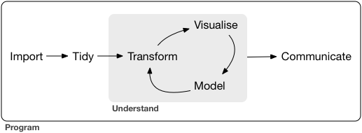
8 |
9 |
10 | # Load tidyverse
11 |
12 | ```{r tidyverse}
13 | library(tidyverse)
14 | library(lubridate)
15 | ```
16 |
17 | # Download
18 |
19 | ```{r download, eval=FALSE}
20 | download.file(
21 | "https://s3.amazonaws.com/nyc-tlc/trip+data/yellow_tripdata_2015-12.csv",
22 | "yellow_tripdata_2015-12.csv")
23 | ```
24 |
25 | # Impord Dataset
26 |
27 | ```{r import, message=FALSE, warning=FALSE}
28 | trips <- read_csv("yellow_tripdata_2015-12.csv", n_max = 1000000)
29 | ```
30 |
31 | # Tidy
32 |
33 | ```{r tidy}
34 | # pickups
35 | select(trips, tpep_pickup_datetime, pickup_latitude, pickup_longitude)
36 |
37 | # dropoffs
38 | select(trips, tpep_dropoff_datetime, dropoff_latitude, dropoff_longitude)
39 |
40 | # trips
41 | trips
42 | ```
43 |
44 | # Transform
45 |
46 | ```{r transform}
47 | tripsHour <- trips %>%
48 | filter(payment_type %in% c(1, 2)) %>%
49 | mutate(pay_type = ifelse(payment_type == 1, "credit", "cash")) %>%
50 | mutate(trip_time_sec = tpep_dropoff_datetime - tpep_pickup_datetime) %>%
51 | mutate(trip_time_min = as.numeric(trip_time_sec / 60)) %>%
52 | mutate(hour = round_date(tpep_pickup_datetime, "hour")) %>%
53 | group_by(pay_type, hour) %>%
54 | summarize(n = n(),
55 | tip_amount = mean(tip_amount),
56 | fare_amount = mean(fare_amount),
57 | passenger_count = mean(passenger_count),
58 | trip_time = mean(trip_time_min),
59 | trip_distance = mean(trip_distance))
60 | tripsHour
61 | ```
62 |
63 | # Visualize
64 |
65 | ```{r visualize}
66 | ggplot(tripsHour, aes(fare_amount, color = pay_type)) +
67 | geom_density() +
68 | labs(title = "NYC taxi fare amount", x = "Fare Amount", y = "Miles", caption = '2015-12')
69 |
70 | qplot(trip_distance, data=tripsHour, geom="density", log="x", facets = ~pay_type)
71 | ```
72 |
73 | # Model
74 |
75 | ```{r model}
76 | # Formula
77 | model_formula <- formula(tip_amount ~ fare_amount + pay_type + passenger_count)
78 |
79 | # Model data
80 | tripsModel <- tripsHour %>%
81 | select(tip_amount, fare_amount, pay_type, passenger_count) %>%
82 | na.omit
83 |
84 | # Linear Model
85 | m1 <- lm(model_formula, data = tripsHour)
86 | summary(m1)
87 |
88 | # Decision tree
89 | library(rpart)
90 | m2 <- rpart(model_formula, tripsHour)
91 | summary(m2)
92 |
93 | # Predict
94 | pred <- tripsHour %>%
95 | ungroup %>%
96 | mutate(lm_fit = predict(m1, tripsHour)) %>%
97 | mutate(lm_res = tip_amount - lm_fit) %>%
98 | mutate(rpart_fit = predict(m2, tripsHour)) %>%
99 | mutate(rpart_res = tip_amount - rpart_fit)
100 |
101 | # MSE
102 | pred %>%
103 | na.omit() %>%
104 | summarize(lm_mse = mean(lm_res^2), rpart_mse = mean(rpart_res^2))
105 |
106 | # Plot
107 | ggplot(pred, aes(rpart_fit, lm_fit)) + geom_point() + geom_smooth(method="lm")
108 | ```
109 |
110 | # Communicate
111 |
112 | This analysis of one month of NYC Taxi data shows that you can predict tip amount as a function of fare amount, pay type, and passenger account. For a detailed explanation of the code you can view this report in the following formats:
113 |
114 | * HTML
115 | * PDF
116 | * Word
117 |
--------------------------------------------------------------------------------
/prod/presentations/cazena/README.md:
--------------------------------------------------------------------------------
1 | # Analyze data with sparklyr
2 |
3 | ## Abstract
4 |
5 | Sparklyr is an R package that lets you analyze data in Spark while using familiar tools in R. Sparklyr supports a complete backend for dplyr, a popular tool for working with data frame objects both in memory and out of memory. You can use dplyr to translate R code into Spark SQL. Sparklyr also supports MLlib so you can run classifiers, regressions, clustering, decision trees, and many more machine learning algorithms on your distributed data in Spark. With sparklyr you can analyze large amounts of data that would not traditionally fit into R memory. Then you can collect results from Spark into R for further visualization and documentation.
6 |
7 |
8 |
--------------------------------------------------------------------------------
/prod/presentations/cazena/emr_setup.sh:
--------------------------------------------------------------------------------
1 | ### Build EMR master node with Taxi Data
2 | ### Nathan Stephens
3 | ### 3/27/2017
4 |
5 | ###########################################
6 | ### Run as root
7 | ###########################################
8 |
9 | ## RSP
10 |
11 | # Upate
12 | sudo yum update
13 |
14 | # R
15 | sudo yum install -y R libcurl-devel openssl-devel git
16 |
17 | # install RSP
18 | wget -q https://download2.rstudio.org/current.ver -O /tmp/rsp.current.ver
19 | wget -O /tmp/rstudio-server-rhel.rpm https://s3.amazonaws.com/rstudio-dailybuilds/rstudio-server-rhel-pro-$(cat /tmp/rsp.current.ver)-x86_64.rpm
20 | sudo yum install -y --nogpgcheck /tmp/rstudio-server-rhel.rpm
21 |
22 | # install packages
23 | sudo Rscript -e 'install.packages("sparklyr", repos = "http://cran.rstudio.com/")'
24 | sudo Rscript -e 'install.packages("devtools", repos = "http://cran.rstudio.com/")'
25 | sudo Rscript -e 'install.packages("tidyverse", repos = "http://cran.rstudio.com/")'
26 | sudo Rscript -e 'install.packages("leaflet", repos = "http://cran.rstudio.com/")'
27 | sudo Rscript -e 'install.packages("DT", repos = "http://cran.rstudio.com/")'
28 |
29 | ###########################################
30 |
31 | ## Add rstudio user
32 | sudo useradd -m rstudio
33 | sudo echo rstudio | passwd rstudio --stdin
34 | sudo usermod -a -G hadoop rstudio
35 | sudo usermod -a -G hive rstudio
36 |
37 |
38 | ###########################################
39 | ### Run as rstudio
40 | ###########################################
41 |
42 | ## switch user
43 | su rstudio
44 | cd ~
45 |
46 | ## add rstudio directory
47 | hadoop fs -mkdir /user/rstudio
48 | hadoop fs -chown rstudio:rstudio /user/rstudio
49 |
50 | ## clone project
51 | git clone https://github.com/rstudio/sparkDemos.git /home/rstudio/sparkDemos
52 | cat >/home/rstudio/sparkDemos/sparkDemos.Rproj <> nyct2010.log &
71 | nohup /usr/bin/s3-dist-cp --src=s3n://rstudio-sparkdemo-data/nyc-taxi/parquet_nohead/trips --dest=hdfs:///user/rstudio/trips_par >> trips_par.log &
72 | nohup /usr/bin/s3-dist-cp --src=s3n://rstudio-sparkdemo-data/nyc-taxi/parquet/trips_model_data --dest=hdfs:///user/rstudio/trips_model_data >> trips_model_data.log &
73 |
74 |
75 | ###########################################
76 | ### Open Hive
77 | ###########################################
78 |
79 | hive
80 |
81 | # Hive 1
82 |
83 | CREATE EXTERNAL TABLE IF NOT EXISTS nyct2010(
84 | gid int,
85 | ctlabel float,
86 | borocode int,
87 | boroname string,
88 | ct2010 int,
89 | boroct2010 int,
90 | cdeligibil string,
91 | ntacode string,
92 | ntaname string,
93 | puma int)
94 | ROW FORMAT DELIMITED
95 | FIELDS TERMINATED BY ','
96 | LINES TERMINATED BY '\n'
97 | ;
98 |
99 | LOAD DATA INPATH '/user/rstudio/nyct2010' INTO TABLE nyct2010;
100 |
101 | # Hive 3
102 |
103 | CREATE EXTERNAL TABLE IF NOT EXISTS trips_par(
104 | id int,
105 | cab_type_id int,
106 | vendor_id string,
107 | pickup_datetime timestamp,
108 | dropoff_datetime timestamp,
109 | store_and_fwd_flag string,
110 | rate_code_id string,
111 | pickup_longitude float,
112 | pickup_latitude float,
113 | dropoff_longitude float,
114 | dropoff_latitude float,
115 | passenger_count bigint,
116 | trip_distance float,
117 | fare_amount float,
118 | extra bigint,
119 | mta_tax string,
120 | tip_amount float,
121 | tolls_amount float,
122 | ehail_fee string,
123 | improvement_surcharge string,
124 | total_amount float,
125 | payment_type string,
126 | trip_type string,
127 | pickup_nyct2010_gid int,
128 | dropoff_nyct2010_gid int)
129 | stored as parquet;
130 |
131 | LOAD DATA INPATH '/user/rstudio/trips_par' INTO TABLE trips_par;
132 |
133 |
134 | # Hive 3
135 | CREATE EXTERNAL TABLE IF NOT EXISTS trips_model_data(
136 | pickup_datetime timestamp,
137 | pickup_latitude float,
138 | pickup_longitude float,
139 | pickup_nyct2010_gid int,
140 | pickup_boro string,
141 | pickup_nta string,
142 | dropoff_datetime timestamp,
143 | dropoff_latitude float,
144 | dropoff_longitude float,
145 | dropoff_nyct2010_gid int,
146 | dropoff_boro string,
147 | dropoff_nta string,
148 | cab_type string,
149 | passenger_count bigint,
150 | trip_distance float,
151 | pay_type string,
152 | fare_amount float,
153 | tip_amount float,
154 | other_amount float,
155 | total_amount float)
156 | stored as parquet;
157 |
158 | LOAD DATA INPATH '/user/rstudio/trips_model_data' INTO TABLE trips_model_data;
159 |
160 |
--------------------------------------------------------------------------------
/prod/presentations/cazena/kerberos.R:
--------------------------------------------------------------------------------
1 | system("echo '' | kinit ")
2 |
--------------------------------------------------------------------------------
/prod/presentations/cazena/sqlvis_histogram.R:
--------------------------------------------------------------------------------
1 | ### Big data histogram
2 | sqlvis_compute_histogram <- function(data, x_name, bins = 30){
3 |
4 | data_prep <- data %>%
5 | select_(x_field = x_name) %>%
6 | filter(!is.na(x_field)) %>%
7 | mutate(x_field = as.double(x_field))
8 |
9 | s <- data_prep %>%
10 | summarise(max_x = max(x_field), min_x = min(x_field)) %>%
11 | mutate(bin_value = (max_x - min_x) / bins) %>%
12 | collect()
13 |
14 | new_bins <- as.numeric(c((0:(bins - 1) * s$bin_value) + s$min_x, s$max_x))
15 |
16 | plot_table <- data_prep %>%
17 | ft_bucketizer(input.col = "x_field", output.col = "key_bin", splits = new_bins) %>%
18 | group_by(key_bin) %>%
19 | tally() %>%
20 | collect()
21 |
22 | all_bins <- data.frame(
23 | key_bin = 0:(bins - 1),
24 | bin = 1:bins,
25 | bin_ceiling = head(new_bins, -1)
26 | )
27 |
28 | plot_table %>%
29 | full_join(all_bins, by="key_bin") %>%
30 | arrange(key_bin) %>%
31 | mutate(n = ifelse(!is.na(n), n, 0)) %>%
32 | select(bin = key_bin, count = n, bin_ceiling) %>%
33 | rename_(.dots = setNames(list("bin_ceiling"), x_name))
34 |
35 | }
36 |
37 | sqlvis_ggplot_histogram <- function(plot_table, ...){
38 | plot_table %>%
39 | select(x = 3, y = 2) %>%
40 | ggplot(aes(x, y)) +
41 | geom_bar(stat = "identity", fill = "cornflowerblue") +
42 | theme(legend.position = "none") +
43 | labs(x = colnames(plot_table)[3], y = colnames(plot_table)[2], ...)
44 | }
45 |
46 | sqlvis_ggvis_histogram <- function(plot_table, ...){
47 | plot_table %>%
48 | select(x = 3, y = 2) %>%
49 | ggvis(x = ~x, y = ~y) %>%
50 | layer_bars() %>%
51 | add_axis("x", title = colnames(plot_table)[3]) %>%
52 | add_axis("y", title = colnames(plot_table)[2])
53 | }
54 |
55 |
--------------------------------------------------------------------------------
/prod/presentations/cazena/sqlvis_raster.R:
--------------------------------------------------------------------------------
1 | ### Big data tile plot
2 |
3 | # data <- tbl(sc, "trips_model_data")
4 | # x_field <- "pickup_longitude"
5 | # y_field <- "pickup_latitude"
6 | # resolution <- 50
7 |
8 | sqlvis_compute_raster <- function(data, x_field, y_field, resolution = 300){
9 |
10 | data_prep <- data %>%
11 | select_(x = x_field, y = y_field) %>%
12 | filter(!is.na(x), !is.na(y))
13 |
14 | s <- data_prep %>%
15 | summarise(max_x = max(x),
16 | max_y = max(y),
17 | min_x = min(x),
18 | min_y = min(y)) %>%
19 | mutate(rng_x = max_x - min_x,
20 | rng_y = max_y - min_y,
21 | resolution = resolution) %>%
22 | collect()
23 |
24 | counts <- data_prep %>%
25 | mutate(res_x = round((x - s$min_x) / s$rng_x * resolution, 0),
26 | res_y = round((y - s$min_y) / s$rng_y * resolution, 0)) %>%
27 | count(res_x, res_y) %>%
28 | collect
29 |
30 | list(counts = counts,
31 | limits = s,
32 | vnames = c(x_field, y_field)
33 | )
34 |
35 | }
36 |
37 | sqlvis_ggplot_raster <- function(data, ...) {
38 |
39 | d <- data$counts
40 | s <- data$limits
41 | v <- data$vnames
42 |
43 | xx <- setNames(seq(1, s$resolution, len = 6), round(seq(s$min_x, s$max_x, len = 6),2))
44 | yy <- setNames(seq(1, s$resolution, len = 6), round(seq(s$min_y, s$max_y, len = 6),2))
45 |
46 | ggplot(d, aes(res_x, res_y)) +
47 | geom_raster(aes(fill = n)) +
48 | coord_fixed() +
49 | scale_fill_distiller(palette = "Spectral", trans = "log", name = "Frequency") +
50 | scale_x_continuous(breaks = xx, labels = names(xx)) +
51 | scale_y_continuous(breaks = yy, labels = names(yy)) +
52 | labs(x = v[1], y = v[2], ...)
53 |
54 | }
55 |
56 | ### Facets
57 |
58 | sqlvis_compute_raster_g <- function(data, x_field, y_field, g_field, resolution = 300){
59 |
60 | data_prep <- data %>%
61 | mutate_(group = g_field) %>%
62 | select_(g = "group", x = x_field, y = y_field) %>%
63 | filter(!is.na(x), !is.na(y))
64 |
65 | s <- data_prep %>%
66 | summarise(max_x = max(x),
67 | max_y = max(y),
68 | min_x = min(x),
69 | min_y = min(y)) %>%
70 | mutate(rng_x = max_x - min_x,
71 | rng_y = max_y - min_y,
72 | resolution = resolution) %>%
73 | collect()
74 |
75 | counts <- data_prep %>%
76 | mutate(res_x = round((x-s$min_x)/s$rng_x*resolution, 0),
77 | res_y = round((y-s$min_y)/s$rng_y*resolution, 0)) %>%
78 | count(g, res_x, res_y) %>%
79 | collect
80 |
81 | list(counts = counts,
82 | limits = s,
83 | vnames = c(x_field, y_field)
84 | )
85 |
86 | }
87 |
88 | sqlvis_ggplot_raster_g <- function(data, ncol = 4, ...) {
89 |
90 | s <- data$limits
91 | d <- data$counts
92 | v <- data$vnames
93 |
94 | xx <- setNames(seq(1, s$resolution, len = 3), round(seq(s$min_x, s$max_x, len = 3), 1))
95 | yy <- setNames(seq(1, s$resolution, len = 3), round(seq(s$min_y, s$max_y, len = 3), 1))
96 |
97 | ggplot(d, aes(res_x, res_y)) +
98 | geom_raster(aes(fill = n)) +
99 | coord_fixed() +
100 | facet_wrap(~ g, ncol = ncol) +
101 | scale_fill_distiller(palette = "Spectral", trans = "log", name = "Frequency") +
102 | scale_x_continuous(breaks = xx, labels = names(xx)) +
103 | scale_y_continuous(breaks = yy, labels = names(yy)) +
104 | labs(x = v[1], y = v[2], ...)
105 |
106 | }
107 |
--------------------------------------------------------------------------------
/prod/presentations/cloudera/livy-architecture.png:
--------------------------------------------------------------------------------
https://raw.githubusercontent.com/rstudio/sparkDemos/7b5c55154ef6513a49889c52c961359e8ab2cf49/prod/presentations/cloudera/livy-architecture.png
--------------------------------------------------------------------------------
/prod/presentations/cloudera/livy.Rmd:
--------------------------------------------------------------------------------
1 | ---
2 | title: "Connecting to Spark through Livy"
3 | output: html_notebook
4 | ---
5 |
6 | With Livy you can anaylze data in your spark cluster via R on your desktop.
7 |
8 | ## Livy
9 |
10 | Livy is a service that enables easy interaction with an Apache Spark cluster over a REST interface. It enables easy submission of Spark jobs or snippets of Spark code, synchronous or asynchronous result retrieval, as well as SparkContext management, all via a simple REST interface or a RPC client library. Livy also simplifies the interaction between Spark from application servers, thus enabling the use of Spark for interactive web/mobile applications.
11 |
12 |
13 | 
14 |
15 |
16 | ## Start Livy
17 |
18 | Set home environment variables and start a Livy server to handle local requests.
19 |
20 | ```{bash}
21 | export JAVA_HOME=/usr/lib/jvm/java-7-oracle-cloudera
22 | export SPARK_HOME=/opt/cloudera/parcels/CDH/lib/spark
23 | /home/ubuntu/livy/livy-server-0.2.0/bin/livy-server
24 | ```
25 |
26 | ## Connect to Spark
27 |
28 | Use `method = "livy"` to connect to the cluster.
29 |
30 | ```{r}
31 | library(sparklyr)
32 | library(dplyr)
33 | sc <- spark_connect(
34 | master = "http://ec2-***.us-west-2.compute.amazonaws.com:8998",
35 | method = "livy")
36 | ```
37 |
38 | ## Analyze
39 |
40 | Use R code on your workstation as you normally would. Your R commands will be sent to the cluster via Livy for processing. Collect your results back to the desktop for further processing in R.
41 |
42 | ```{r}
43 | library(ggplot2)
44 | trips_model_data_tbl <- tbl(sc, "trips_model_data")
45 | pickup_dropoff_tbl <- trips_model_data_tbl %>%
46 | filter(pickup_nta == "Turtle Bay-East Midtown" & dropoff_nta == "Airport") %>%
47 | mutate(pickup_hour = hour(pickup_datetime)) %>%
48 | mutate(trip_time = unix_timestamp(dropoff_datetime) - unix_timestamp(pickup_datetime)) %>%
49 | group_by(pickup_hour) %>%
50 | summarize(n = n(),
51 | trip_time_mean = mean(trip_time),
52 | trip_time_p10 = percentile(trip_time, 0.10),
53 | trip_time_p25 = percentile(trip_time, 0.25),
54 | trip_time_p50 = percentile(trip_time, 0.50),
55 | trip_time_p75 = percentile(trip_time, 0.75),
56 | trip_time_p90 = percentile(trip_time, 0.90))
57 |
58 | # Collect results
59 | pickup_dropoff <- collect(pickup_dropoff_tbl)
60 |
61 | # Plot
62 | ggplot(pickup_dropoff, aes(x = pickup_hour)) +
63 | geom_line(aes(y = trip_time_p50, alpha = "Median")) +
64 | geom_ribbon(aes(ymin = trip_time_p25, ymax = trip_time_p75,
65 | alpha = "25–75th percentile")) +
66 | geom_ribbon(aes(ymin = trip_time_p10, ymax = trip_time_p90,
67 | alpha = "10–90th percentile")) +
68 | scale_y_continuous("trip duration in minutes")
69 | ```
70 |
--------------------------------------------------------------------------------
/prod/presentations/cloudera/readme.md:
--------------------------------------------------------------------------------
1 | # Demo using CDH 5.9
2 |
3 | This repos contains files for demonstrating Spark and R on Cloudera using spakrlyr.
4 |
5 | ### Scripts
6 |
7 | * Taxi Demo
8 | * Livy Connection
9 | * Histogram wrappers
10 | * Raster wrappers
11 |
12 | ### Reports
13 |
14 | * [Data Science Toolchain with Spark and R](http://colorado.rstudio.com:3939/content/262/taxiDemoCloudera3.nb.html)
15 | * [Connecting to Spark through Livy](http://colorado.rstudio.com:3939/content/259/livy.nb.html)
16 |
17 | ### Reference
18 |
19 | * [spark.rstudio.com](http://spark.rstudio.com/)
--------------------------------------------------------------------------------
/prod/presentations/cloudera/sqlvis_histogram.R:
--------------------------------------------------------------------------------
1 | ### Big data histogram
2 | sqlvis_compute_histogram <- function(data, x_name, bins = 30){
3 |
4 | data_prep <- data %>%
5 | select_(x_field = x_name) %>%
6 | filter(!is.na(x_field)) %>%
7 | mutate(x_field = as.double(x_field))
8 |
9 | s <- data_prep %>%
10 | summarise(max_x = max(x_field), min_x = min(x_field)) %>%
11 | mutate(bin_value = (max_x - min_x) / bins) %>%
12 | collect()
13 |
14 | new_bins <- as.numeric(c((0:(bins - 1) * s$bin_value) + s$min_x, s$max_x))
15 |
16 | plot_table <- data_prep %>%
17 | ft_bucketizer(input.col = "x_field", output.col = "key_bin", splits = new_bins) %>%
18 | group_by(key_bin) %>%
19 | tally() %>%
20 | collect()
21 |
22 | all_bins <- data.frame(
23 | key_bin = 0:(bins - 1),
24 | bin = 1:bins,
25 | bin_ceiling = head(new_bins, -1)
26 | )
27 |
28 | plot_table %>%
29 | full_join(all_bins, by="key_bin") %>%
30 | arrange(key_bin) %>%
31 | mutate(n = ifelse(!is.na(n), n, 0)) %>%
32 | select(bin = key_bin, count = n, bin_ceiling) %>%
33 | rename_(.dots = setNames(list("bin_ceiling"), x_name))
34 |
35 | }
36 |
37 | sqlvis_ggplot_histogram <- function(plot_table, ...){
38 | plot_table %>%
39 | select(x = 3, y = 2) %>%
40 | ggplot(aes(x, y)) +
41 | geom_bar(stat = "identity", fill = "cornflowerblue") +
42 | theme(legend.position = "none") +
43 | labs(x = colnames(plot_table)[3], y = colnames(plot_table)[2], ...)
44 | }
45 |
46 | sqlvis_ggvis_histogram <- function(plot_table, ...){
47 | plot_table %>%
48 | select(x = 3, y = 2) %>%
49 | ggvis(x = ~x, y = ~y) %>%
50 | layer_bars() %>%
51 | add_axis("x", title = colnames(plot_table)[3]) %>%
52 | add_axis("y", title = colnames(plot_table)[2])
53 | }
54 |
55 |
--------------------------------------------------------------------------------
/prod/presentations/cloudera/sqlvis_raster.R:
--------------------------------------------------------------------------------
1 | ### Big data tile plot
2 |
3 | # data <- tbl(sc, "trips_model_data")
4 | # x_field <- "pickup_longitude"
5 | # y_field <- "pickup_latitude"
6 | # resolution <- 50
7 |
8 | sqlvis_compute_raster <- function(data, x_field, y_field, resolution = 300){
9 |
10 | data_prep <- data %>%
11 | select_(x = x_field, y = y_field) %>%
12 | filter(!is.na(x), !is.na(y))
13 |
14 | s <- data_prep %>%
15 | summarise(max_x = max(x),
16 | max_y = max(y),
17 | min_x = min(x),
18 | min_y = min(y)) %>%
19 | mutate(rng_x = max_x - min_x,
20 | rng_y = max_y - min_y,
21 | resolution = resolution) %>%
22 | collect()
23 |
24 | counts <- data_prep %>%
25 | mutate(res_x = round((x - s$min_x) / s$rng_x * resolution, 0),
26 | res_y = round((y - s$min_y) / s$rng_y * resolution, 0)) %>%
27 | count(res_x, res_y) %>%
28 | collect
29 |
30 | list(counts = counts,
31 | limits = s,
32 | vnames = c(x_field, y_field)
33 | )
34 |
35 | }
36 |
37 | sqlvis_ggplot_raster <- function(data, ...) {
38 |
39 | d <- data$counts
40 | s <- data$limits
41 | v <- data$vnames
42 |
43 | xx <- setNames(seq(1, s$resolution, len = 6), round(seq(s$min_x, s$max_x, len = 6),2))
44 | yy <- setNames(seq(1, s$resolution, len = 6), round(seq(s$min_y, s$max_y, len = 6),2))
45 |
46 | ggplot(d, aes(res_x, res_y)) +
47 | geom_raster(aes(fill = n)) +
48 | coord_fixed() +
49 | scale_fill_distiller(palette = "Spectral", trans = "log", name = "Frequency") +
50 | scale_x_continuous(breaks = xx, labels = names(xx)) +
51 | scale_y_continuous(breaks = yy, labels = names(yy)) +
52 | labs(x = v[1], y = v[2], ...)
53 |
54 | }
55 |
56 | ### Facets
57 |
58 | sqlvis_compute_raster_g <- function(data, x_field, y_field, g_field, resolution = 300){
59 |
60 | data_prep <- data %>%
61 | mutate_(group = g_field) %>%
62 | select_(g = "group", x = x_field, y = y_field) %>%
63 | filter(!is.na(x), !is.na(y))
64 |
65 | s <- data_prep %>%
66 | summarise(max_x = max(x),
67 | max_y = max(y),
68 | min_x = min(x),
69 | min_y = min(y)) %>%
70 | mutate(rng_x = max_x - min_x,
71 | rng_y = max_y - min_y,
72 | resolution = resolution) %>%
73 | collect()
74 |
75 | counts <- data_prep %>%
76 | mutate(res_x = round((x-s$min_x)/s$rng_x*resolution, 0),
77 | res_y = round((y-s$min_y)/s$rng_y*resolution, 0)) %>%
78 | count(g, res_x, res_y) %>%
79 | collect
80 |
81 | list(counts = counts,
82 | limits = s,
83 | vnames = c(x_field, y_field)
84 | )
85 |
86 | }
87 |
88 | sqlvis_ggplot_raster_g <- function(data, ncol = 4, ...) {
89 |
90 | s <- data$limits
91 | d <- data$counts
92 | v <- data$vnames
93 |
94 | xx <- setNames(seq(1, s$resolution, len = 3), round(seq(s$min_x, s$max_x, len = 3), 1))
95 | yy <- setNames(seq(1, s$resolution, len = 3), round(seq(s$min_y, s$max_y, len = 3), 1))
96 |
97 | ggplot(d, aes(res_x, res_y)) +
98 | geom_raster(aes(fill = n)) +
99 | coord_fixed() +
100 | facet_wrap(~ g, ncol = ncol) +
101 | scale_fill_distiller(palette = "Spectral", trans = "log", name = "Frequency") +
102 | scale_x_continuous(breaks = xx, labels = names(xx)) +
103 | scale_y_continuous(breaks = yy, labels = names(yy)) +
104 | labs(x = v[1], y = v[2], ...)
105 |
106 | }
107 |
--------------------------------------------------------------------------------
/prod/presentations/sparkSummitEast/README.md:
--------------------------------------------------------------------------------
1 | # Analyze data with sparklyr
2 |
3 | ## Abstract
4 |
5 | Sparklyr is an R package that lets you analyze data in Spark while using familiar tools in R. Sparklyr supports a complete backend for dplyr, a popular tool for working with data frame objects both in memory and out of memory. You can use dplyr to translate R code into Spark SQL. Sparklyr also supports MLlib so you can run classifiers, regressions, clustering, decision trees, and many more machine learning algorithms on your distributed data in Spark. With sparklyr you can analyze large amounts of data that would not traditionally fit into R memory. Then you can collect results from Spark into R for further visualization and documentation.
6 |
7 | Sparklyr is also extensible. You can create R packages that depend on sparklyr to call the full Spark API. One example of an extension is H2O’s rsparkling, an R package that works with H2O’s machine learning algorithm. With sparklyr and rsparkling you have access to all the tools in H2O for analysis with R and Spark.
8 |
9 | ## Documents
10 |
11 | * [Data Science Toolchain with Spark and R](http://colorado.rstudio.com:3939/content/276/taxiDemoH2O.nb.html)
12 | * [Connecting to Spark through Livy](http://colorado.rstudio.com:3939/content/289/livy.nb.html)
13 |
14 | ## Slides
15 |
16 | 
17 |
18 | ***
19 |
20 | 
21 |
22 | ***
23 |
24 | 
25 |
26 | ***
27 |
28 | 
29 |
30 | ***
31 |
32 | 
33 |
34 | ***
35 |
36 | 
37 |
38 | ***
39 |
40 | 
41 |
42 | ***
43 |
44 | 
45 |
46 | ***
47 |
48 | 
49 |
50 | ***
51 |
52 | 
53 |
54 | ***
55 |
56 | 
57 |
58 | ***
59 |
60 | 
61 |
62 | ***
63 |
64 | 
65 |
66 | ***
67 |
68 | 
69 |
70 | ***
71 |
72 | 
73 |
74 | ***
75 |
76 | 
77 |
78 | ***
79 |
80 | 
81 |
--------------------------------------------------------------------------------
/prod/presentations/sparkSummitEast/img/img.001.jpeg:
--------------------------------------------------------------------------------
https://raw.githubusercontent.com/rstudio/sparkDemos/7b5c55154ef6513a49889c52c961359e8ab2cf49/prod/presentations/sparkSummitEast/img/img.001.jpeg
--------------------------------------------------------------------------------
/prod/presentations/sparkSummitEast/img/img.002.jpeg:
--------------------------------------------------------------------------------
https://raw.githubusercontent.com/rstudio/sparkDemos/7b5c55154ef6513a49889c52c961359e8ab2cf49/prod/presentations/sparkSummitEast/img/img.002.jpeg
--------------------------------------------------------------------------------
/prod/presentations/sparkSummitEast/img/img.003.jpeg:
--------------------------------------------------------------------------------
https://raw.githubusercontent.com/rstudio/sparkDemos/7b5c55154ef6513a49889c52c961359e8ab2cf49/prod/presentations/sparkSummitEast/img/img.003.jpeg
--------------------------------------------------------------------------------
/prod/presentations/sparkSummitEast/img/img.004.jpeg:
--------------------------------------------------------------------------------
https://raw.githubusercontent.com/rstudio/sparkDemos/7b5c55154ef6513a49889c52c961359e8ab2cf49/prod/presentations/sparkSummitEast/img/img.004.jpeg
--------------------------------------------------------------------------------
/prod/presentations/sparkSummitEast/img/img.005.jpeg:
--------------------------------------------------------------------------------
https://raw.githubusercontent.com/rstudio/sparkDemos/7b5c55154ef6513a49889c52c961359e8ab2cf49/prod/presentations/sparkSummitEast/img/img.005.jpeg
--------------------------------------------------------------------------------
/prod/presentations/sparkSummitEast/img/img.006.jpeg:
--------------------------------------------------------------------------------
https://raw.githubusercontent.com/rstudio/sparkDemos/7b5c55154ef6513a49889c52c961359e8ab2cf49/prod/presentations/sparkSummitEast/img/img.006.jpeg
--------------------------------------------------------------------------------
/prod/presentations/sparkSummitEast/img/img.007.jpeg:
--------------------------------------------------------------------------------
https://raw.githubusercontent.com/rstudio/sparkDemos/7b5c55154ef6513a49889c52c961359e8ab2cf49/prod/presentations/sparkSummitEast/img/img.007.jpeg
--------------------------------------------------------------------------------
/prod/presentations/sparkSummitEast/img/img.008.jpeg:
--------------------------------------------------------------------------------
https://raw.githubusercontent.com/rstudio/sparkDemos/7b5c55154ef6513a49889c52c961359e8ab2cf49/prod/presentations/sparkSummitEast/img/img.008.jpeg
--------------------------------------------------------------------------------
/prod/presentations/sparkSummitEast/img/img.009.jpeg:
--------------------------------------------------------------------------------
https://raw.githubusercontent.com/rstudio/sparkDemos/7b5c55154ef6513a49889c52c961359e8ab2cf49/prod/presentations/sparkSummitEast/img/img.009.jpeg
--------------------------------------------------------------------------------
/prod/presentations/sparkSummitEast/img/img.010.jpeg:
--------------------------------------------------------------------------------
https://raw.githubusercontent.com/rstudio/sparkDemos/7b5c55154ef6513a49889c52c961359e8ab2cf49/prod/presentations/sparkSummitEast/img/img.010.jpeg
--------------------------------------------------------------------------------
/prod/presentations/sparkSummitEast/img/img.011.jpeg:
--------------------------------------------------------------------------------
https://raw.githubusercontent.com/rstudio/sparkDemos/7b5c55154ef6513a49889c52c961359e8ab2cf49/prod/presentations/sparkSummitEast/img/img.011.jpeg
--------------------------------------------------------------------------------
/prod/presentations/sparkSummitEast/img/img.012.jpeg:
--------------------------------------------------------------------------------
https://raw.githubusercontent.com/rstudio/sparkDemos/7b5c55154ef6513a49889c52c961359e8ab2cf49/prod/presentations/sparkSummitEast/img/img.012.jpeg
--------------------------------------------------------------------------------
/prod/presentations/sparkSummitEast/img/img.013.jpeg:
--------------------------------------------------------------------------------
https://raw.githubusercontent.com/rstudio/sparkDemos/7b5c55154ef6513a49889c52c961359e8ab2cf49/prod/presentations/sparkSummitEast/img/img.013.jpeg
--------------------------------------------------------------------------------
/prod/presentations/sparkSummitEast/img/img.014.jpeg:
--------------------------------------------------------------------------------
https://raw.githubusercontent.com/rstudio/sparkDemos/7b5c55154ef6513a49889c52c961359e8ab2cf49/prod/presentations/sparkSummitEast/img/img.014.jpeg
--------------------------------------------------------------------------------
/prod/presentations/sparkSummitEast/img/img.015.jpeg:
--------------------------------------------------------------------------------
https://raw.githubusercontent.com/rstudio/sparkDemos/7b5c55154ef6513a49889c52c961359e8ab2cf49/prod/presentations/sparkSummitEast/img/img.015.jpeg
--------------------------------------------------------------------------------
/prod/presentations/sparkSummitEast/img/img.016.jpeg:
--------------------------------------------------------------------------------
https://raw.githubusercontent.com/rstudio/sparkDemos/7b5c55154ef6513a49889c52c961359e8ab2cf49/prod/presentations/sparkSummitEast/img/img.016.jpeg
--------------------------------------------------------------------------------
/prod/presentations/sparkSummitEast/img/img.017.jpeg:
--------------------------------------------------------------------------------
https://raw.githubusercontent.com/rstudio/sparkDemos/7b5c55154ef6513a49889c52c961359e8ab2cf49/prod/presentations/sparkSummitEast/img/img.017.jpeg
--------------------------------------------------------------------------------
/prod/presentations/sparkSummitEast/livy.Rmd:
--------------------------------------------------------------------------------
1 | ---
2 | title: "Connecting to Spark through Livy"
3 | output: html_notebook
4 | ---
5 |
6 | With Livy you can anaylze data in your spark cluster via R on your desktop.
7 |
8 | ## Livy
9 |
10 | Livy is a service that enables easy interaction with an Apache Spark cluster over a REST interface. It enables easy submission of Spark jobs or snippets of Spark code, synchronous or asynchronous result retrieval, as well as SparkContext management, all via a simple REST interface or a RPC client library. Livy also simplifies the interaction between Spark from application servers, thus enabling the use of Spark for interactive web/mobile applications.
11 |
12 |
13 | 
14 |
15 |
16 | ## Start Livy [Server Side]
17 |
18 | Set home environment variables and start a Livy server to handle local requests.
19 |
20 | ```{r, eval=FALSE}
21 | sparklyr::livy_install()
22 | sparklyr::livy_service_start()
23 | ```
24 |
25 | ## Connect to Spark [Client Side]
26 |
27 | Use `method = "livy"` to connect to the cluster.
28 |
29 | ```{r warning=FALSE, eval=FALSE}
30 | library(sparklyr)
31 | library(dplyr)
32 | sc <- spark_connect(
33 | master = "http://ec2-***-**-***-**.compute-1.amazonaws.com:8998/",
34 | method = "livy")
35 | ```
36 |
37 | ## Analyze [Client Side]
38 |
39 | Use R code on your workstation as you normally would. Your R commands will be sent to the cluster via Livy for processing. Collect your results back to the desktop for further processing in R.
40 |
41 | ```{r eval=FALSE}
42 | library(ggplot2)
43 | trips_model_data_tbl <- tbl(sc, "trips_model_data")
44 | pickup_dropoff_tbl <- trips_model_data_tbl %>%
45 | filter(pickup_nta == "Turtle Bay-East Midtown" & dropoff_nta == "Airport") %>%
46 | mutate(pickup_hour = hour(pickup_datetime)) %>%
47 | mutate(trip_time = unix_timestamp(dropoff_datetime) - unix_timestamp(pickup_datetime)) %>%
48 | group_by(pickup_hour) %>%
49 | summarize(n = n(),
50 | trip_time_mean = mean(trip_time),
51 | trip_time_p10 = percentile(trip_time, 0.10),
52 | trip_time_p25 = percentile(trip_time, 0.25),
53 | trip_time_p50 = percentile(trip_time, 0.50),
54 | trip_time_p75 = percentile(trip_time, 0.75),
55 | trip_time_p90 = percentile(trip_time, 0.90))
56 |
57 | # Collect results
58 | pickup_dropoff <- collect(pickup_dropoff_tbl)
59 |
60 | # Plot
61 | ggplot(pickup_dropoff, aes(x = pickup_hour)) +
62 | geom_line(aes(y = trip_time_p50, alpha = "Median")) +
63 | geom_ribbon(aes(ymin = trip_time_p25, ymax = trip_time_p75,
64 | alpha = "25–75th percentile")) +
65 | geom_ribbon(aes(ymin = trip_time_p10, ymax = trip_time_p90,
66 | alpha = "10–90th percentile")) +
67 | scale_y_continuous("trip duration in minutes")
68 | ```
69 |
70 | ## Disconnect [Sever Side]
71 |
72 | ```{r disconnect, eval=FALSE}
73 | sparklyr::livy_service_stop()
74 | ```
75 |
76 |
77 |
--------------------------------------------------------------------------------
/prod/presentations/sparkSummitEast/sqlvis_histogram.R:
--------------------------------------------------------------------------------
1 | ### Big data histogram
2 | sqlvis_compute_histogram <- function(data, x_name, bins = 30){
3 |
4 | data_prep <- data %>%
5 | select_(x_field = x_name) %>%
6 | filter(!is.na(x_field)) %>%
7 | mutate(x_field = as.double(x_field))
8 |
9 | s <- data_prep %>%
10 | summarise(max_x = max(x_field), min_x = min(x_field)) %>%
11 | mutate(bin_value = (max_x - min_x) / bins) %>%
12 | collect()
13 |
14 | new_bins <- as.numeric(c((0:(bins - 1) * s$bin_value) + s$min_x, s$max_x))
15 |
16 | plot_table <- data_prep %>%
17 | ft_bucketizer(input.col = "x_field", output.col = "key_bin", splits = new_bins) %>%
18 | group_by(key_bin) %>%
19 | tally() %>%
20 | collect()
21 |
22 | all_bins <- data.frame(
23 | key_bin = 0:(bins - 1),
24 | bin = 1:bins,
25 | bin_ceiling = head(new_bins, -1)
26 | )
27 |
28 | plot_table %>%
29 | full_join(all_bins, by="key_bin") %>%
30 | arrange(key_bin) %>%
31 | mutate(n = ifelse(!is.na(n), n, 0)) %>%
32 | select(bin = key_bin, count = n, bin_ceiling) %>%
33 | rename_(.dots = setNames(list("bin_ceiling"), x_name))
34 |
35 | }
36 |
37 | sqlvis_ggplot_histogram <- function(plot_table, ...){
38 | plot_table %>%
39 | select(x = 3, y = 2) %>%
40 | ggplot(aes(x, y)) +
41 | geom_bar(stat = "identity", fill = "cornflowerblue") +
42 | theme(legend.position = "none") +
43 | labs(x = colnames(plot_table)[3], y = colnames(plot_table)[2], ...)
44 | }
45 |
46 | sqlvis_ggvis_histogram <- function(plot_table, ...){
47 | plot_table %>%
48 | select(x = 3, y = 2) %>%
49 | ggvis(x = ~x, y = ~y) %>%
50 | layer_bars() %>%
51 | add_axis("x", title = colnames(plot_table)[3]) %>%
52 | add_axis("y", title = colnames(plot_table)[2])
53 | }
54 |
55 |
--------------------------------------------------------------------------------
/prod/presentations/sparkSummitEast/sqlvis_raster.R:
--------------------------------------------------------------------------------
1 | ### Big data tile plot
2 |
3 | # data <- tbl(sc, "trips_model_data")
4 | # x_field <- "pickup_longitude"
5 | # y_field <- "pickup_latitude"
6 | # resolution <- 50
7 |
8 | sqlvis_compute_raster <- function(data, x_field, y_field, resolution = 300){
9 |
10 | data_prep <- data %>%
11 | select_(x = x_field, y = y_field) %>%
12 | filter(!is.na(x), !is.na(y))
13 |
14 | s <- data_prep %>%
15 | summarise(max_x = max(x),
16 | max_y = max(y),
17 | min_x = min(x),
18 | min_y = min(y)) %>%
19 | mutate(rng_x = max_x - min_x,
20 | rng_y = max_y - min_y,
21 | resolution = resolution) %>%
22 | collect()
23 |
24 | counts <- data_prep %>%
25 | mutate(res_x = round((x - s$min_x) / s$rng_x * resolution, 0),
26 | res_y = round((y - s$min_y) / s$rng_y * resolution, 0)) %>%
27 | count(res_x, res_y) %>%
28 | collect
29 |
30 | list(counts = counts,
31 | limits = s,
32 | vnames = c(x_field, y_field)
33 | )
34 |
35 | }
36 |
37 | sqlvis_ggplot_raster <- function(data, ...) {
38 |
39 | d <- data$counts
40 | s <- data$limits
41 | v <- data$vnames
42 |
43 | xx <- setNames(seq(1, s$resolution, len = 6), round(seq(s$min_x, s$max_x, len = 6),2))
44 | yy <- setNames(seq(1, s$resolution, len = 6), round(seq(s$min_y, s$max_y, len = 6),2))
45 |
46 | ggplot(d, aes(res_x, res_y)) +
47 | geom_raster(aes(fill = n)) +
48 | coord_fixed() +
49 | scale_fill_distiller(palette = "Spectral", trans = "log", name = "Frequency") +
50 | scale_x_continuous(breaks = xx, labels = names(xx)) +
51 | scale_y_continuous(breaks = yy, labels = names(yy)) +
52 | labs(x = v[1], y = v[2], ...)
53 |
54 | }
55 |
56 | ### Facets
57 |
58 | sqlvis_compute_raster_g <- function(data, x_field, y_field, g_field, resolution = 300){
59 |
60 | data_prep <- data %>%
61 | mutate_(group = g_field) %>%
62 | select_(g = "group", x = x_field, y = y_field) %>%
63 | filter(!is.na(x), !is.na(y))
64 |
65 | s <- data_prep %>%
66 | summarise(max_x = max(x),
67 | max_y = max(y),
68 | min_x = min(x),
69 | min_y = min(y)) %>%
70 | mutate(rng_x = max_x - min_x,
71 | rng_y = max_y - min_y,
72 | resolution = resolution) %>%
73 | collect()
74 |
75 | counts <- data_prep %>%
76 | mutate(res_x = round((x-s$min_x)/s$rng_x*resolution, 0),
77 | res_y = round((y-s$min_y)/s$rng_y*resolution, 0)) %>%
78 | count(g, res_x, res_y) %>%
79 | collect
80 |
81 | list(counts = counts,
82 | limits = s,
83 | vnames = c(x_field, y_field)
84 | )
85 |
86 | }
87 |
88 | sqlvis_ggplot_raster_g <- function(data, ncol = 4, ...) {
89 |
90 | s <- data$limits
91 | d <- data$counts
92 | v <- data$vnames
93 |
94 | xx <- setNames(seq(1, s$resolution, len = 3), round(seq(s$min_x, s$max_x, len = 3), 1))
95 | yy <- setNames(seq(1, s$resolution, len = 3), round(seq(s$min_y, s$max_y, len = 3), 1))
96 |
97 | ggplot(d, aes(res_x, res_y)) +
98 | geom_raster(aes(fill = n)) +
99 | coord_fixed() +
100 | facet_wrap(~ g, ncol = ncol) +
101 | scale_fill_distiller(palette = "Spectral", trans = "log", name = "Frequency") +
102 | scale_x_continuous(breaks = xx, labels = names(xx)) +
103 | scale_y_continuous(breaks = yy, labels = names(yy)) +
104 | labs(x = v[1], y = v[2], ...)
105 |
106 | }
107 |
--------------------------------------------------------------------------------
/prod/presentations/tidyverse/01_taxiR.Rmd:
--------------------------------------------------------------------------------
1 | ---
2 | title: "NYC Taxi - One month in R"
3 | output: html_notebook
4 | ---
5 |
6 |
7 | 
8 |
9 |
10 | # Load tidyverse
11 |
12 | ```{r tidyverse}
13 | library(tidyverse)
14 | library(lubridate)
15 | ```
16 |
17 | # Download
18 |
19 | ```{r download, eval=FALSE}
20 | download.file(
21 | "https://s3.amazonaws.com/nyc-tlc/trip+data/yellow_tripdata_2015-12.csv",
22 | "yellow_tripdata_2015-12.csv")
23 | ```
24 |
25 | # Impord Dataset
26 |
27 | ```{r import, message=FALSE, warning=FALSE}
28 | trips <- read_csv("~/sparkDemos/prod/presentations/tidyverse/yellow_tripdata_2015-12.csv")
29 | ```
30 |
31 | # Tidy
32 |
33 | ```{r tidy}
34 | # pickups
35 | select(trips, tpep_pickup_datetime, pickup_latitude, pickup_longitude)
36 |
37 | # dropoffs
38 | select(trips, tpep_dropoff_datetime, dropoff_latitude, dropoff_longitude)
39 |
40 | # trips
41 | trips
42 | ```
43 |
44 | # Transform
45 |
46 | ```{r transform}
47 | tripsHour <- trips %>%
48 | filter(payment_type %in% c(1, 2)) %>%
49 | mutate(pay_type = ifelse(payment_type == 1, "credit", "cash")) %>%
50 | mutate(trip_time_sec = tpep_dropoff_datetime - tpep_pickup_datetime) %>%
51 | mutate(trip_time_min = as.numeric(trip_time_sec / 60)) %>%
52 | mutate(hour = round_date(tpep_pickup_datetime, "hour")) %>%
53 | group_by(pay_type, hour) %>%
54 | summarize(n = n(),
55 | tip_amount = mean(tip_amount),
56 | fare_amount = mean(fare_amount),
57 | passenger_count = mean(passenger_count),
58 | trip_time = mean(trip_time_min),
59 | trip_distance = mean(trip_distance))
60 | tripsHour
61 | ```
62 |
63 | # Visualize
64 |
65 | ```{r visualize}
66 | ggplot(tripsHour, aes(trip_time, trip_distance, color = pay_type)) +
67 | geom_point() + geom_smooth() +
68 | labs(title = "NYC Taxi by hour by day", x = "Minutes", y = "Miles", caption = '2015-12')
69 |
70 | ggplot(tripsHour, aes(trip_distance, fare_amount)) +
71 | geom_point() + geom_smooth() + facet_grid(~pay_type) +
72 | labs(title = "NYC Taxi by hour by day", x = "Distance", y = "Dollars", caption = '2015-12')
73 | ```
74 |
75 | # Model
76 |
77 | ```{r model}
78 | # Formula
79 | model_formula <- formula(tip_amount ~ fare_amount + pay_type + passenger_count)
80 |
81 | # Model data
82 | tripsModel <- tripsHour %>%
83 | select(tip_amount, fare_amount, pay_type, passenger_count) %>%
84 | na.omit
85 |
86 | # Linear Model
87 | m1 <- lm(model_formula, data = tripsHour)
88 | summary(m1)
89 |
90 | # Decision tree
91 | library(rpart)
92 | m2 <- rpart(model_formula, tripsHour)
93 | summary(m2)
94 |
95 | # Predict
96 | pred <- tripsHour %>%
97 | ungroup %>%
98 | mutate(lm_fit = predict(m1, tripsHour)) %>%
99 | mutate(lm_res = tip_amount - lm_fit) %>%
100 | mutate(rpart_fit = predict(m2, tripsHour)) %>%
101 | mutate(rpart_res = tip_amount - rpart_fit)
102 |
103 | # MSE
104 | pred %>%
105 | na.omit() %>%
106 | summarize(lm_mse = mean(lm_res^2), rpart_mse = mean(rpart_res^2))
107 |
108 | # Plot
109 | ggplot(pred, aes(rpart_fit, lm_fit)) + geom_point() + geom_smooth(method="lm")
110 | ```
111 |
112 | # Communicate
113 |
114 | This analysis of one month of NYC Taxi data shows that you can predict tip amount as a function of fare amount, pay type, and passenger account. For a detailed explanation of the code you can view this report in the following formats:
115 |
116 | * HTML
117 | * PDF
118 | * Word
119 |
--------------------------------------------------------------------------------
/prod/presentations/tidyverse/README.md:
--------------------------------------------------------------------------------
1 | # Analyze data with sparklyr
2 |
3 | ## Abstract
4 |
5 | Sparklyr is an R package that lets you analyze data in Spark while using familiar tools in R. Sparklyr supports a complete backend for dplyr, a popular tool for working with data frame objects both in memory and out of memory. You can use dplyr to translate R code into Spark SQL. Sparklyr also supports MLlib so you can run classifiers, regressions, clustering, decision trees, and many more machine learning algorithms on your distributed data in Spark. With sparklyr you can analyze large amounts of data that would not traditionally fit into R memory. Then you can collect results from Spark into R for further visualization and documentation.
6 |
7 | ## Documents
8 |
9 | These documents are for understanding the toolchain and the tidyverse using the famous NYC taxi data.
10 |
11 | * [Data Science Toolchain with Spark and R](http://colorado.rstudio.com:3939/content/420/taxiDemo.nb.html)
12 | * [Tidyverse and R Notebooks with NYC Taxi Data](http://colorado.rstudio.com:3939/content/421/taxiR.nb.html)
13 |
14 | ## Slides
15 |
16 | 
17 |
18 | ***
19 |
20 | 
21 |
22 | ***
23 |
24 | 
25 |
26 | ***
27 |
28 | 
29 |
30 | ***
31 |
32 | 
33 |
34 | ***
35 |
36 | 
37 |
38 | ***
39 |
40 | 
41 |
42 | ***
43 |
44 | 
45 |
46 | ***
47 |
48 | 
49 |
50 | ***
51 |
52 | 
53 |
54 | ***
55 |
56 | 
57 |
58 | ***
59 |
60 | 
61 |
62 | ***
63 |
64 | 
65 |
66 | ***
67 |
68 | 
69 |
70 | ***
71 |
72 | 
73 |
74 | ***
75 |
76 | 
77 |
78 |
--------------------------------------------------------------------------------
/prod/presentations/tidyverse/emr_setup.sh:
--------------------------------------------------------------------------------
1 | ### Build EMR master node with Taxi Data
2 | ### Nathan Stephens
3 | ### 3/27/2017
4 |
5 | ###########################################
6 | ### Run as root
7 | ###########################################
8 |
9 | ## RSP
10 |
11 | # Upate
12 | sudo yum update
13 |
14 | # R
15 | sudo yum install -y R libcurl-devel openssl-devel git
16 |
17 | # install RSP
18 | wget -q https://download2.rstudio.org/current.ver -O /tmp/rsp.current.ver
19 | wget -O /tmp/rstudio-server-rhel.rpm https://s3.amazonaws.com/rstudio-dailybuilds/rstudio-server-rhel-pro-$(cat /tmp/rsp.current.ver)-x86_64.rpm
20 | sudo yum install -y --nogpgcheck /tmp/rstudio-server-rhel.rpm
21 |
22 | # install packages
23 | sudo Rscript -e 'install.packages("sparklyr", repos = "http://cran.rstudio.com/")'
24 | sudo Rscript -e 'install.packages("devtools", repos = "http://cran.rstudio.com/")'
25 | sudo Rscript -e 'install.packages("tidyverse", repos = "http://cran.rstudio.com/")'
26 | sudo Rscript -e 'install.packages("leaflet", repos = "http://cran.rstudio.com/")'
27 | sudo Rscript -e 'install.packages("DT", repos = "http://cran.rstudio.com/")'
28 |
29 | ###########################################
30 |
31 | ## Add rstudio user
32 | sudo useradd -m rstudio
33 | sudo echo rstudio | passwd rstudio --stdin
34 | sudo usermod -a -G hadoop rstudio
35 | sudo usermod -a -G hive rstudio
36 |
37 |
38 | ###########################################
39 | ### Run as rstudio
40 | ###########################################
41 |
42 | ## switch user
43 | su rstudio
44 | cd ~
45 |
46 | ## add rstudio directory
47 | hadoop fs -mkdir /user/rstudio
48 | hadoop fs -chown rstudio:rstudio /user/rstudio
49 |
50 | ## clone project
51 | git clone https://github.com/rstudio/sparkDemos.git /home/rstudio/sparkDemos
52 | cat >/home/rstudio/sparkDemos/sparkDemos.Rproj <> nyct2010.log &
71 | nohup /usr/bin/s3-dist-cp --src=s3n://rstudio-sparkdemo-data/nyc-taxi/parquet_nohead/trips --dest=hdfs:///user/rstudio/trips_par >> trips_par.log &
72 | nohup /usr/bin/s3-dist-cp --src=s3n://rstudio-sparkdemo-data/nyc-taxi/parquet/trips_model_data --dest=hdfs:///user/rstudio/trips_model_data >> trips_model_data.log &
73 |
74 |
75 | ###########################################
76 | ### Open Hive
77 | ###########################################
78 |
79 | hive
80 |
81 | # Hive 1
82 |
83 | CREATE EXTERNAL TABLE IF NOT EXISTS nyct2010(
84 | gid int,
85 | ctlabel float,
86 | borocode int,
87 | boroname string,
88 | ct2010 int,
89 | boroct2010 int,
90 | cdeligibil string,
91 | ntacode string,
92 | ntaname string,
93 | puma int)
94 | ROW FORMAT DELIMITED
95 | FIELDS TERMINATED BY ','
96 | LINES TERMINATED BY '\n'
97 | ;
98 |
99 | LOAD DATA INPATH '/user/rstudio/nyct2010' INTO TABLE nyct2010;
100 |
101 | # Hive 3
102 |
103 | CREATE EXTERNAL TABLE IF NOT EXISTS trips_par(
104 | id int,
105 | cab_type_id int,
106 | vendor_id string,
107 | pickup_datetime timestamp,
108 | dropoff_datetime timestamp,
109 | store_and_fwd_flag string,
110 | rate_code_id string,
111 | pickup_longitude float,
112 | pickup_latitude float,
113 | dropoff_longitude float,
114 | dropoff_latitude float,
115 | passenger_count bigint,
116 | trip_distance float,
117 | fare_amount float,
118 | extra bigint,
119 | mta_tax string,
120 | tip_amount float,
121 | tolls_amount float,
122 | ehail_fee string,
123 | improvement_surcharge string,
124 | total_amount float,
125 | payment_type string,
126 | trip_type string,
127 | pickup_nyct2010_gid int,
128 | dropoff_nyct2010_gid int)
129 | stored as parquet;
130 |
131 | LOAD DATA INPATH '/user/rstudio/trips_par' INTO TABLE trips_par;
132 |
133 |
134 | # Hive 3
135 | CREATE EXTERNAL TABLE IF NOT EXISTS trips_model_data(
136 | pickup_datetime timestamp,
137 | pickup_latitude float,
138 | pickup_longitude float,
139 | pickup_nyct2010_gid int,
140 | pickup_boro string,
141 | pickup_nta string,
142 | dropoff_datetime timestamp,
143 | dropoff_latitude float,
144 | dropoff_longitude float,
145 | dropoff_nyct2010_gid int,
146 | dropoff_boro string,
147 | dropoff_nta string,
148 | cab_type string,
149 | passenger_count bigint,
150 | trip_distance float,
151 | pay_type string,
152 | fare_amount float,
153 | tip_amount float,
154 | other_amount float,
155 | total_amount float)
156 | stored as parquet;
157 |
158 | LOAD DATA INPATH '/user/rstudio/trips_model_data' INTO TABLE trips_model_data;
159 |
160 |
--------------------------------------------------------------------------------
/prod/presentations/tidyverse/img/tidyverse.001.jpeg:
--------------------------------------------------------------------------------
https://raw.githubusercontent.com/rstudio/sparkDemos/7b5c55154ef6513a49889c52c961359e8ab2cf49/prod/presentations/tidyverse/img/tidyverse.001.jpeg
--------------------------------------------------------------------------------
/prod/presentations/tidyverse/img/tidyverse.002.jpeg:
--------------------------------------------------------------------------------
https://raw.githubusercontent.com/rstudio/sparkDemos/7b5c55154ef6513a49889c52c961359e8ab2cf49/prod/presentations/tidyverse/img/tidyverse.002.jpeg
--------------------------------------------------------------------------------
/prod/presentations/tidyverse/img/tidyverse.003.jpeg:
--------------------------------------------------------------------------------
https://raw.githubusercontent.com/rstudio/sparkDemos/7b5c55154ef6513a49889c52c961359e8ab2cf49/prod/presentations/tidyverse/img/tidyverse.003.jpeg
--------------------------------------------------------------------------------
/prod/presentations/tidyverse/img/tidyverse.004.jpeg:
--------------------------------------------------------------------------------
https://raw.githubusercontent.com/rstudio/sparkDemos/7b5c55154ef6513a49889c52c961359e8ab2cf49/prod/presentations/tidyverse/img/tidyverse.004.jpeg
--------------------------------------------------------------------------------
/prod/presentations/tidyverse/img/tidyverse.005.jpeg:
--------------------------------------------------------------------------------
https://raw.githubusercontent.com/rstudio/sparkDemos/7b5c55154ef6513a49889c52c961359e8ab2cf49/prod/presentations/tidyverse/img/tidyverse.005.jpeg
--------------------------------------------------------------------------------
/prod/presentations/tidyverse/img/tidyverse.006.jpeg:
--------------------------------------------------------------------------------
https://raw.githubusercontent.com/rstudio/sparkDemos/7b5c55154ef6513a49889c52c961359e8ab2cf49/prod/presentations/tidyverse/img/tidyverse.006.jpeg
--------------------------------------------------------------------------------
/prod/presentations/tidyverse/img/tidyverse.007.jpeg:
--------------------------------------------------------------------------------
https://raw.githubusercontent.com/rstudio/sparkDemos/7b5c55154ef6513a49889c52c961359e8ab2cf49/prod/presentations/tidyverse/img/tidyverse.007.jpeg
--------------------------------------------------------------------------------
/prod/presentations/tidyverse/img/tidyverse.008.jpeg:
--------------------------------------------------------------------------------
https://raw.githubusercontent.com/rstudio/sparkDemos/7b5c55154ef6513a49889c52c961359e8ab2cf49/prod/presentations/tidyverse/img/tidyverse.008.jpeg
--------------------------------------------------------------------------------
/prod/presentations/tidyverse/img/tidyverse.009.jpeg:
--------------------------------------------------------------------------------
https://raw.githubusercontent.com/rstudio/sparkDemos/7b5c55154ef6513a49889c52c961359e8ab2cf49/prod/presentations/tidyverse/img/tidyverse.009.jpeg
--------------------------------------------------------------------------------
/prod/presentations/tidyverse/img/tidyverse.010.jpeg:
--------------------------------------------------------------------------------
https://raw.githubusercontent.com/rstudio/sparkDemos/7b5c55154ef6513a49889c52c961359e8ab2cf49/prod/presentations/tidyverse/img/tidyverse.010.jpeg
--------------------------------------------------------------------------------
/prod/presentations/tidyverse/img/tidyverse.011.jpeg:
--------------------------------------------------------------------------------
https://raw.githubusercontent.com/rstudio/sparkDemos/7b5c55154ef6513a49889c52c961359e8ab2cf49/prod/presentations/tidyverse/img/tidyverse.011.jpeg
--------------------------------------------------------------------------------
/prod/presentations/tidyverse/img/tidyverse.012.jpeg:
--------------------------------------------------------------------------------
https://raw.githubusercontent.com/rstudio/sparkDemos/7b5c55154ef6513a49889c52c961359e8ab2cf49/prod/presentations/tidyverse/img/tidyverse.012.jpeg
--------------------------------------------------------------------------------
/prod/presentations/tidyverse/img/tidyverse.013.jpeg:
--------------------------------------------------------------------------------
https://raw.githubusercontent.com/rstudio/sparkDemos/7b5c55154ef6513a49889c52c961359e8ab2cf49/prod/presentations/tidyverse/img/tidyverse.013.jpeg
--------------------------------------------------------------------------------
/prod/presentations/tidyverse/img/tidyverse.014.jpeg:
--------------------------------------------------------------------------------
https://raw.githubusercontent.com/rstudio/sparkDemos/7b5c55154ef6513a49889c52c961359e8ab2cf49/prod/presentations/tidyverse/img/tidyverse.014.jpeg
--------------------------------------------------------------------------------
/prod/presentations/tidyverse/img/tidyverse.015.jpeg:
--------------------------------------------------------------------------------
https://raw.githubusercontent.com/rstudio/sparkDemos/7b5c55154ef6513a49889c52c961359e8ab2cf49/prod/presentations/tidyverse/img/tidyverse.015.jpeg
--------------------------------------------------------------------------------
/prod/presentations/tidyverse/img/tidyverse.016.jpeg:
--------------------------------------------------------------------------------
https://raw.githubusercontent.com/rstudio/sparkDemos/7b5c55154ef6513a49889c52c961359e8ab2cf49/prod/presentations/tidyverse/img/tidyverse.016.jpeg
--------------------------------------------------------------------------------
/prod/presentations/tidyverse/sqlvis_histogram.R:
--------------------------------------------------------------------------------
1 | ### Big data histogram
2 | sqlvis_compute_histogram <- function(data, x_name, bins = 30){
3 |
4 | data_prep <- data %>%
5 | select_(x_field = x_name) %>%
6 | filter(!is.na(x_field)) %>%
7 | mutate(x_field = as.double(x_field))
8 |
9 | s <- data_prep %>%
10 | summarise(max_x = max(x_field), min_x = min(x_field)) %>%
11 | mutate(bin_value = (max_x - min_x) / bins) %>%
12 | collect()
13 |
14 | new_bins <- as.numeric(c((0:(bins - 1) * s$bin_value) + s$min_x, s$max_x))
15 |
16 | plot_table <- data_prep %>%
17 | ft_bucketizer(input.col = "x_field", output.col = "key_bin", splits = new_bins) %>%
18 | group_by(key_bin) %>%
19 | tally() %>%
20 | collect()
21 |
22 | all_bins <- data.frame(
23 | key_bin = 0:(bins - 1),
24 | bin = 1:bins,
25 | bin_ceiling = head(new_bins, -1)
26 | )
27 |
28 | plot_table %>%
29 | full_join(all_bins, by="key_bin") %>%
30 | arrange(key_bin) %>%
31 | mutate(n = ifelse(!is.na(n), n, 0)) %>%
32 | select(bin = key_bin, count = n, bin_ceiling) %>%
33 | rename_(.dots = setNames(list("bin_ceiling"), x_name))
34 |
35 | }
36 |
37 | sqlvis_ggplot_histogram <- function(plot_table, ...){
38 | plot_table %>%
39 | select(x = 3, y = 2) %>%
40 | ggplot(aes(x, y)) +
41 | geom_bar(stat = "identity", fill = "cornflowerblue") +
42 | theme(legend.position = "none") +
43 | labs(x = colnames(plot_table)[3], y = colnames(plot_table)[2], ...)
44 | }
45 |
46 | sqlvis_ggvis_histogram <- function(plot_table, ...){
47 | plot_table %>%
48 | select(x = 3, y = 2) %>%
49 | ggvis(x = ~x, y = ~y) %>%
50 | layer_bars() %>%
51 | add_axis("x", title = colnames(plot_table)[3]) %>%
52 | add_axis("y", title = colnames(plot_table)[2])
53 | }
54 |
55 |
--------------------------------------------------------------------------------
/prod/presentations/tidyverse/sqlvis_raster.R:
--------------------------------------------------------------------------------
1 | ### Big data tile plot
2 |
3 | # data <- tbl(sc, "trips_model_data")
4 | # x_field <- "pickup_longitude"
5 | # y_field <- "pickup_latitude"
6 | # resolution <- 50
7 |
8 | sqlvis_compute_raster <- function(data, x_field, y_field, resolution = 300){
9 |
10 | data_prep <- data %>%
11 | select_(x = x_field, y = y_field) %>%
12 | filter(!is.na(x), !is.na(y))
13 |
14 | s <- data_prep %>%
15 | summarise(max_x = max(x),
16 | max_y = max(y),
17 | min_x = min(x),
18 | min_y = min(y)) %>%
19 | mutate(rng_x = max_x - min_x,
20 | rng_y = max_y - min_y,
21 | resolution = resolution) %>%
22 | collect()
23 |
24 | counts <- data_prep %>%
25 | mutate(res_x = round((x - s$min_x) / s$rng_x * resolution, 0),
26 | res_y = round((y - s$min_y) / s$rng_y * resolution, 0)) %>%
27 | count(res_x, res_y) %>%
28 | collect
29 |
30 | list(counts = counts,
31 | limits = s,
32 | vnames = c(x_field, y_field)
33 | )
34 |
35 | }
36 |
37 | sqlvis_ggplot_raster <- function(data, ...) {
38 |
39 | d <- data$counts
40 | s <- data$limits
41 | v <- data$vnames
42 |
43 | xx <- setNames(seq(1, s$resolution, len = 6), round(seq(s$min_x, s$max_x, len = 6),2))
44 | yy <- setNames(seq(1, s$resolution, len = 6), round(seq(s$min_y, s$max_y, len = 6),2))
45 |
46 | ggplot(d, aes(res_x, res_y)) +
47 | geom_raster(aes(fill = n)) +
48 | coord_fixed() +
49 | scale_fill_distiller(palette = "Spectral", trans = "log", name = "Frequency") +
50 | scale_x_continuous(breaks = xx, labels = names(xx)) +
51 | scale_y_continuous(breaks = yy, labels = names(yy)) +
52 | labs(x = v[1], y = v[2], ...)
53 |
54 | }
55 |
56 | ### Facets
57 |
58 | sqlvis_compute_raster_g <- function(data, x_field, y_field, g_field, resolution = 300){
59 |
60 | data_prep <- data %>%
61 | mutate_(group = g_field) %>%
62 | select_(g = "group", x = x_field, y = y_field) %>%
63 | filter(!is.na(x), !is.na(y))
64 |
65 | s <- data_prep %>%
66 | summarise(max_x = max(x),
67 | max_y = max(y),
68 | min_x = min(x),
69 | min_y = min(y)) %>%
70 | mutate(rng_x = max_x - min_x,
71 | rng_y = max_y - min_y,
72 | resolution = resolution) %>%
73 | collect()
74 |
75 | counts <- data_prep %>%
76 | mutate(res_x = round((x-s$min_x)/s$rng_x*resolution, 0),
77 | res_y = round((y-s$min_y)/s$rng_y*resolution, 0)) %>%
78 | count(g, res_x, res_y) %>%
79 | collect
80 |
81 | list(counts = counts,
82 | limits = s,
83 | vnames = c(x_field, y_field)
84 | )
85 |
86 | }
87 |
88 | sqlvis_ggplot_raster_g <- function(data, ncol = 4, ...) {
89 |
90 | s <- data$limits
91 | d <- data$counts
92 | v <- data$vnames
93 |
94 | xx <- setNames(seq(1, s$resolution, len = 3), round(seq(s$min_x, s$max_x, len = 3), 1))
95 | yy <- setNames(seq(1, s$resolution, len = 3), round(seq(s$min_y, s$max_y, len = 3), 1))
96 |
97 | ggplot(d, aes(res_x, res_y)) +
98 | geom_raster(aes(fill = n)) +
99 | coord_fixed() +
100 | facet_wrap(~ g, ncol = ncol) +
101 | scale_fill_distiller(palette = "Spectral", trans = "log", name = "Frequency") +
102 | scale_x_continuous(breaks = xx, labels = names(xx)) +
103 | scale_y_continuous(breaks = yy, labels = names(yy)) +
104 | labs(x = v[1], y = v[2], ...)
105 |
106 | }
107 |
--------------------------------------------------------------------------------
/prod/presentations/tidyverse/tidyverseAndSpark.pdf:
--------------------------------------------------------------------------------
https://raw.githubusercontent.com/rstudio/sparkDemos/7b5c55154ef6513a49889c52c961359e8ab2cf49/prod/presentations/tidyverse/tidyverseAndSpark.pdf
--------------------------------------------------------------------------------