├── README.md
├── binary-search
└── binary-search.md
├── bits-and-subsets
└── bits-and-subsets.md
├── data-structures
└── introduction
│ └── introduction.md
├── dynamic-programming
├── bitmask-dynamic-programming
│ └── bitmask-dynamic-programming.md
└── introduction
│ └── introduction.md
├── graph-theory
├── introduction
│ └── introduction.md
├── shortest-path
│ └── dijkstras-algorithm
│ │ └── dijkstras-algorithm.md
└── traversal
│ ├── breadth-first-search
│ ├── BreadthFirstSearch.java
│ └── breadth-first-search.md
│ └── depth-first-search
│ ├── DepthFirstSearch.java
│ └── depth-first-search.md
├── problem-solving
└── problem-solving.md
└── resources
├── binary-search.png
├── graph-theory-dijkstras-algorithm-1.png
├── graph-theory-dijkstras-algorithm-2.png
├── graph-theory-dijkstras-algorithm-3.png
├── graph-theory-introduction-1.png
├── graph-theory-introduction-2.png
└── graph-theory-introduction-3.png
/README.md:
--------------------------------------------------------------------------------
1 | # Data Structures and Algorithms
2 |
3 | ## Introduction
4 |
5 | This repository contains notes that have been converted from slideshows I created in college for the University of Florida Programming Team. I plan on adding notes for the more advanced topics I did not get to while at college. If you have any questions, requests, or find an error in the provided notes, please feel free to either open an issue or contact me at cormacpayne@ufl.edu
6 |
7 | ## Websites for Practice
8 |
9 | Below are websites I recommend for practicing contests and individual problems
10 |
11 | - [Sphere Online Judge (SPOJ)](http://www.spoj.com/)
12 | - [Codeforces](http://codeforces.com/)
13 | - [Topcoder](https://www.topcoder.com/)
14 | - [UVa Online Judge](https://uva.onlinejudge.org/)
15 | - [Kattis](https://open.kattis.com/)
16 | - [HackerRank](https://www.hackerrank.com/)
17 |
18 | ## Books
19 |
20 | Below are books that I recommend reading if you are interested in learning more about competitive programming, as well as data structures and algorithms
21 |
22 | - [Competitive Programming, 3rd Edition - Steven Halim](https://www.amazon.com/Competitive-Programming-3rd-Steven-Halim/dp/B00FG8MNN8)
23 | - [The Algorithm Design Manual, 2nd Edition - Steven Skiena](https://www.amazon.com/Algorithm-Design-Manual-Steven-Skiena/dp/1848000693/ref=sr_1_1?s=books&ie=UTF8&qid=1484196474&sr=1-1&keywords=the+algorithm+design+manual)
24 | - [Introduction to Graph Theory, 2nd Edition - Richard Trudeau](https://www.amazon.com/Introduction-Graph-Theory-Dover-Mathematics/dp/0486678709)
25 | - [Introductory Graph Theory - Gary Chartrand](https://www.amazon.com/Introductory-Graph-Theory-Dover-Mathematics/dp/0486247759/ref=pd_sim_14_25?_encoding=UTF8&pd_rd_i=0486247759&pd_rd_r=D7Q9XSGFQ9J1TGQTYCZ0&pd_rd_w=KswGa&pd_rd_wg=0ayQt&psc=1&refRID=D7Q9XSGFQ9J1TGQTYCZ0)
26 |
27 | ## Completed Notes
28 |
29 | ### Getting Started
30 |
31 | - [Introduction to Problem Solving](./problem-solving)
32 | - [Basic Data Structures](./data-structures/introduction)
33 | - [Bits and Subsets](./bits-and-subsets.md)
34 | - [Binary Search](./binary-search.md)
35 |
36 | ### Graph Theory
37 |
38 | - [Introduction to Graph Theory](./graph-theory/introduction)
39 | - [Breadth-First Search](./graph-theory/traversal/breadth-first-search)
40 | - [Depth-First Search](./graph-theory/traversal/depth-first-search)
41 | - [Dijkstra's Algorithm](./graph-theory/shortest-path/dijkstras-algorithm)
42 |
43 | ### Dynamic Programming
44 |
45 | - [Introduction to Dynamic Programming](./dynamic-programming/introduction)
46 | - [Bitmask Dynamic Programming](./dynamic-programming/bitmask-dynamic-programming)
47 |
48 | ## Wish List
49 |
50 | ### Graph Theory
51 |
52 | - Minimum Spanning Tree
53 | - Prim's Algorithm
54 | - Kruskal's Algorithm
55 | - Boruvka's Algorithm
56 | - All Pairs Shortest Path
57 | - Floyd Warshall Algorithm
58 | - Single Source Shortest Path
59 | - Bellman-Ford Algorithm
60 | - Heavy-Light Decomposition
61 | - Strongly Connected Components
62 | - Other
63 | - Vertex Cover
64 | - Edge Coloring
65 | - Euler Tour
66 | - Hamiltonian Cycle
67 | - Max Flow
68 | - Ford-Fulkerson Algorithm
69 | - Dinic's Algorithm
70 | - Push-Relabel Algorithm
71 | - Min-Cost Max-Flow
72 | - Maximum Bipartite Matching
73 | - Hungarian Algorithm
74 |
75 | ### Geometry
76 |
77 | - Convex Hull
78 | - Rotating Calipers
79 | - Sweep Line
80 |
81 | ### Number Theory
82 |
83 | - Sieve of Eratosthenes
84 |
85 | ### String Algorithms
86 |
87 | - Knuth-Morris-Pratt Algorithm
88 | - Boyer-Moore Algorithm
89 | - Longest Common Substring/Subsequence
90 | - Shortest Common Superstring
91 | - Palindromes
92 |
93 | ### Data Structures
94 |
95 | - String Data Structures
96 | - Suffix Tree/Array
97 | - Trie
98 | - Segment Trees
99 | - Binary Indexed Trees
100 | - Binary Search Trees
101 | - Kd Trees
102 |
--------------------------------------------------------------------------------
/binary-search/binary-search.md:
--------------------------------------------------------------------------------
1 | # Binary Search
2 |
3 | ## Motivating Problem I
4 |
5 | Imagine that you have a phone book and want to find your friend's phone number.
6 |
7 | With so many people listed, how do you efficiently search for your friend's last name?
8 |
9 | ## Motivating Problem II
10 |
11 | You ask your friend to think of a number between 1 and 100; you attempt to guess what number they're thinking of, and they will tell you if the number you guessed is bigger or smaller than their number.
12 |
13 | You keep doing this until you successfully find their number; the number of guesses you had is your score, so you attempt to minimize your score.
14 |
15 | Since there are only 100 numbers, your score should be relatively small, but what if you told your friend to think of a number between 1 and 1,000,000?
16 |
17 | How can we quickly find what number they are thinking of?
18 |
19 | ## Definition
20 |
21 | One of the fundamental algorithms in computer science, the *binary search* algorithm is used to quickly find a value in a sorted sequence.
22 |
23 | The algorithm works by repeatedly dividing in half the portion of the sequence that could contain the target value, until you've narrowed down the possible locations to just one.
24 |
25 | ## Time Complexity
26 |
27 | Suppose we have a sorted sequence of 32 numbers.
28 |
29 | If we randomly guess, the maximum number of guesses that it will take to find the target number will be 32.
30 |
31 | If we use binary search, the maximum number of guesses that it will take to find the target number will be 5.
32 | - Remember that every guess eliminates half of the remaining sequence
33 |
34 | Now, suppose we have a sorted sequence of **_N_** numbers.
35 |
36 | If we randomly guess, the maximum number of guesses that it will take to find the target number will be **_N_**.
37 |
38 | If we use binary search, the maximum number of guesses that it will take to find the target number will be **_log(N)_**.
39 |
40 | How much faster is **_log(N)_** than **_N_**?
41 |
42 | | **_N_** | **_log(N)_** |
43 | | ------------- | ------------ |
44 | | 10 | ~3 |
45 | | 100 | ~7 |
46 | | 10,000 | ~13 |
47 | | 1,000,000 | ~20 |
48 | | 1,000,000,000 | ~30 |
49 |
50 | ## Pseudocode
51 |
52 | Let's say that we want to code the binary search algorithm to find a target value in a sorted array of numbers.
53 |
54 | We will use two variables, `lo` and `hi`, to represent the indices of the first and last element of the section of the array that we are currently looking at.
55 |
56 | Let's call the index of the middle number in this target section `mid`, which can be found by finding the average of `lo` and `hi`.
57 |
58 | There are three possible scenarios:
59 |
60 | 1: `array[mid] == targetValue`
61 |
62 | If the middle number of our current sequence is equal to the target value, we have found what we are looking for and are done
63 |
64 | 2: `array[mid] < targetValue`
65 |
66 | If the middle number of our sequence is less than the target value, then we know that the bottom half of the current sequence can be eliminated.
67 |
68 | We can adjust the sequence by setting `lo = mid`
69 |
70 | 3: `array[mid] > targetValue`
71 |
72 | If the middle number of our sequence is greater than the target value, then we know that the top half of the current sequence can be eliminated.
73 |
74 | We can adjust the sequence by setting `hi = mid`
75 |
76 | Now that we have the three possible scenarios handled, we just need to define when to terminate the loop if we never found our target value.
77 |
78 | We want to keep searching while we have some range of numbers to check, so if `lo` ever becomes greater than `hi`, then our target value is not in the array due to the fact that we have run out of numbers to check.
79 |
80 | 
81 |
82 | ## Problems
83 |
84 | - [Hacking the random number generator](http://www.spoj.com/problems/HACKRNDM/)
85 | - [Pizzamania](http://www.spoj.com/problems/OPCPIZZA/)
86 | - [Aggressive cows](http://www.spoj.com/problems/AGGRCOW)
87 | - [ABCDEF](http://www.spoj.com/problems/ABCDEF)
88 | - [Subset Sums](http://www.spoj.com/problems/SUBSUMS/)
89 | - [Cutting Cheese](icpc.kattis.com/problems/cheese)
90 | - [Mountain Walking](http://www.spoj.com/problems/MTWALK/)
91 |
--------------------------------------------------------------------------------
/bits-and-subsets/bits-and-subsets.md:
--------------------------------------------------------------------------------
1 | # Bits and Subsets
2 |
3 | ## What is a bit?
4 |
5 | A _bit_ is the basic unit of information in computing.
6 |
7 | A bit can only have two values: **0** or **1**
8 |
9 | The two values for a bit can also be referred as _true_ or _false_, _on_ or _off_, etc.
10 |
11 | Numbers can be represented using bits: **base-2 (or binary)**
12 |
13 | ## Binary Numbers
14 |
15 | Numbers that we see on a daily basis are said to be represented in _base 10_, called their _decimal representation_ (_e.g._, 32, -3949, 10000, 0)
16 |
17 | _Binary numbers_, which are expressed in _base-2_, are numbers that are composed of only **0s** and **1s**.
18 |
19 | 1610 == 100002
20 |
21 | 5410 == 1101102
22 |
23 | ### Converting from Binary to Decimal
24 |
25 | 1. List out the powers of two above each bit, going right to left
26 | 2. For each bit in the binary number, if the value of the bit is a one, add its corresponding power of two to a running sum
27 | 3. After going through all of the bits, the running sum will be the _base-10_ representation of the number
28 |
29 | For example, let's convert 10011012 to a _base-10_ number:
30 |
31 | | 64 | 32 | 16 | 8 | 4 | 2 | 1 |
32 | |---|---|---|---|---|---|---|
33 | | 1 | 0 | 0 | 1 | 1 | 0 | 1 |
34 |
35 | For each bit that is a one, we will add their corresponding power of two to a running sum.
36 |
37 | **64** + 0 + 0 + **8** + **4** + 0 + **1** = 77
38 |
39 | ### Converting from Decimal to Binary
40 |
41 | 1. Divide the number by two
42 | 2. Write down the remainder (either **0** or **1**)
43 | 3. If the number is non-zero, go back to step 1
44 | 4. The last remainder is the first bit in the _base-2_ representation of the number, the second to last remainder is the second bit, etc.
45 |
46 | For example, let's convert 8110 to a _base-2_ number:
47 |
48 | 81 mod 2 = 1 81 / 2 = 40
49 | 40 mod 2 = 0 40 / 2 = 20
50 | 20 mod 2 = 0 20 / 2 = 10
51 | 10 mod 2 = 0 10 / 2 = 5
52 | 5 mod 2 = 1 5 / 2 = 2
53 | 2 mod 2 = 0 2 / 2 = 1
54 | 1 mod 2 = 1 1 / 2 = 0
55 |
56 | We then read the remainders in reverse order to get the _base-2_ representation of 81: **10100012**
57 |
58 | ## Bitwise Operations
59 |
60 | ### NOT
61 |
62 | The bitwise _NOT_, or complement, is an operation that performs _negation_, which means bits that are zero become one, and those that are one become zero.
63 |
64 | For example,
65 | 1011001 --> 0100110
66 | 1111111 --> 0000000
67 | 1000000 --> 0111111
68 |
69 | In Java, the bitwise _NOT_ is represented by the '~' character.
70 |
71 | ```java
72 | int result = ~32; // 31
73 | ```
74 |
75 | ### AND
76 |
77 | The bitwise _AND_ is an operation between two binary numbers that performs the _logical AND_ operation on each pair of the corresponding bits, which means that if both bits are one, the resulting bit is one, and any other combination of bits results in a zero bit.
78 |
79 | | | 1 | 0 |
80 | |---|---|---|
81 | | **1** | 1 | 0 |
82 | | **0** | 0 | 0 |
83 |
84 | In Java, the bitwise _AND_ is represented by the '&' character.
85 |
86 | ```java
87 | int result = 102 & 53; // 36
88 | ```
89 |
90 | For example, let's look at 102 & 53
91 |
92 | ### OR
93 |
94 | The bitwise _OR_ is an operation between two binary numbers that performs the _logical OR_ operation on each pair of corresponding bits, which means that if both bits are zero, the resulting bit is zero, and any other combination results of bits results in a one bit.
95 |
96 | | | 1 | 0 |
97 | |---|---|---|
98 | | **1** | 1 | 1 |
99 | | **0** | 1 | 0 |
100 |
101 | In Java, the bitwise _OR_ is represented by the '|' character.
102 |
103 | ```java
104 | int result = 102 | 53; // 119
105 | ```
106 |
107 | ### XOR
108 |
109 | The bitwise _XOR_ is an operation between two binary numbers that performs the _logical XOR_ operation on each pair of corresponding bits, which means that if both bits are _different_, the resulting bit is one, and if the bits are the same, the resulting bit is zero.
110 |
111 | | | 1 | 0 |
112 | |---|---|---|
113 | | **1** | 0 | 1 |
114 | | **0** | 1 | 0 |
115 |
116 | In Java, the bitwise _XOR_ is represented by the '^' character.
117 |
118 | ```java
119 | int result = 102 ^ 53; // 83
120 | ```
121 |
122 | ## Bit Shifting
123 |
124 | The _bit shift_ operation moves (or shifts) bits to the left or right in a binary number.
125 |
126 | In Java, a _left-shift_ is denoted by '<<', and a _right-shift_ is denoted by '>>'.
127 |
128 | You will also need to declare how many bits you want to shift a number by.
129 |
130 | For example:
131 | 1012 << 2 == 101002
132 | 1001012 >> 3 == 1002
133 | 12 << 5 == 1000002
134 |
135 | Let's look at the following pattern of bit shifts:
136 | 12 << 0 == 12 == 110
137 | 12 << 1 == 102 == 210
138 | 12 << 2 == 1002 == 410
139 | 12 << 3 == 10002 == 810
140 |
141 | Based on this pattern, we can come up with the following rule:
142 |
143 | 12 << k == 2k
144 |
145 | ## Subsets
146 |
147 | Let _A_ = {2, 3, 5, 7}, and let _B_ be a subset of _A_.
148 |
149 | _B_ is a subset of _A_ if all elements in _B_ are also elements in _A_.
150 |
151 | The following are possible values for _B_:
152 | _B_ = {2, 3, 5}
153 | _B_ = {5, 7}
154 | _B_ = {2, 3, 5, 7}
155 | _B_ = { }
156 |
157 | ### Number of Subsets
158 |
159 | For each element in _S_, we have two choices:
160 | - put the element in our subset
161 | - don't put the element in our subset
162 |
163 | Because we have two choices per element, the total number of subsets that we can have can be calculated with 2_N_, where _N_ is the number of elements in _S_.
164 |
165 | In order to create a subset, we either _take_ or _ignore_ an element in the set. Because there are two choices for each element, we can model a subset using a _binary string_ of length _N_.
166 |
167 | For a bit at some index _k_ in our binary string
168 | - if the bit at index _k_ is zero, then our subset _does not_ contain the _k__th_ element
169 | - if the bit at index _k_ is one, thjen our subset _does_ contain the _k__th_ element
170 |
171 | If we have a set _S_ = {2, 3, 5, 8}, there are four elements in this set, so we will need to create a binary string containing _N_ = 4 bits.
172 |
173 | | 0 | 1 | 2 | 3 |
174 | |---|---|---|---|
175 | | 2 | 3 | 5 | 8 |
176 |
177 | Let's look at different subsets and their binary string representations
178 |
179 | | Subset | Binary | Decimal |
180 | |---|---|---|
181 | | {3, 8} | 1010 | 10 |
182 | | {2, 3} | 0011 | 3 |
183 | | {2, 3, 5, 8} | 1111 | 15 |
184 | | { } | 0000 | 0 |
185 |
186 | ### Subset Iteration
187 |
188 | How can we easily iterate over _all_ subsets of a set _S_ with _N_ elements?
189 |
190 | We know that an _empty_ subset has a binary string of 000...0002 which is 010
191 |
192 | We also know that a _full_ subset has a binary string of 111...1112 which is 2_N_ - 1
193 |
194 | Now that we know all subsets fal in the range of [0, 2_N_ - 1], we can iterate over all numbers in this range to get all of tyhe subsets of our set _S_.
195 |
196 | Recall that 1 << _N_ == 2_N_
197 |
198 | ```java
199 | for ( int subset = 0; subset < ( 1 << N ); subset++ )
200 | {
201 | // This for-loop will find every subset of a set
202 | }
203 | ```
204 |
205 | Given a binary string, how can we check if the bit at index _k_ is a zero or one?
206 |
207 | | 7 | 6 | 5 | 4 | 3 | 2 | 1 | 0 |
208 | |---|---|---|---|---|---|---|---|
209 | | 1 | 0 | 0 | X | 0 | 1 | 1 | 1 |
210 |
211 | Let's say we want to see if the bit at _k_ = 4 is zero or one, we will use the bitwise _AND_ and left-shifting to get our answer.
212 |
213 | Since we are only worried about the bit at _k_ = 4, we can make a separate binary string that only has the bit at _k_ = 4 turned on.
214 |
215 | | 7 | 6 | 5 | 4 | 3 | 2 | 1 | 0 |
216 | |---|---|---|---|---|---|---|---|
217 | | 1 | 0 | 0 | X | 0 | 1 | 1 | 1 |
218 | | 0 | 0 | 0 | 1 | 0 | 0 | 0 | 0 |
219 |
220 | We will then _AND_ these binary strings together, which will result in the binary string 000X0000
221 |
222 | This will result in one of two things:
223 | - if X is zero, then the decimal representation of the binary string will be zero
224 | - if X is one, then the decimal representation of the binary string will be non-zero
225 |
226 | ```java
227 | int leftShift = 1 << k;
228 | int result = subset & leftShift;
229 | if ( result == 0)
230 | // the bit at index k is zero
231 | else
232 | // the bit at index k is one
233 | ```
234 |
235 | We now know how to use the current value of subset to find which elements are in our subset:
236 |
237 | ```java
238 | for ( int subset = 0; subset < ( 1 << N ); subset++ )
239 | {
240 | for ( int k = 0; k < N; k++ )
241 | {
242 | int result = ( 1 << k ) & subset;
243 | if ( result != 0 )
244 | // the item at index k is in the current subset
245 | }
246 | }
247 | ```
248 |
--------------------------------------------------------------------------------
/data-structures/introduction/introduction.md:
--------------------------------------------------------------------------------
1 | # Data Structures
2 |
3 | ## What is a data structure?
4 |
5 | A data structure is a particular way of organizing data in a computer so that it can be used efficiently.
6 |
7 | When a problem becomes very complicated, it becomes useful to have some structure to store data in memory.
8 |
9 | ## Array
10 |
11 | A collection of elements, each identitifed by an array index or key
12 |
13 | ### Example
14 |
15 | ```java
16 | int[] array = new int[5];
17 |
18 | int array = {2, 3, 5, 7, 11};
19 |
20 | System.out.print(array[2]); // output is '5'
21 |
22 | array[2] = 13; // changes the '5' to '13'
23 | ```
24 |
25 | ## Linked Lists
26 |
27 | A list can hold an arbitrary number of items, and can easily change size to add or remove items.
28 |
29 | Each element in the list is called a *node*, and contains two pieces of information:
30 | - **data** - information that the node is holding
31 | - **nextNode** - a reference to the node that follows the current one
32 |
33 | An example class for the **nodes** would look like the following:
34 |
35 | ```java
36 | class Node
37 | {
38 | String data;
39 | Node nextNode;
40 | }
41 | ```
42 |
43 | ### Example
44 |
45 | The following code shows how to create a basic linked list (no data)
46 |
47 | ```java
48 | Node start = new Node();
49 |
50 | for (int i = 1; i <= 10; i++)
51 | {
52 | start.nextNode = new Node();
53 | start = start.nextNode;
54 | }
55 | ```
56 |
57 | The following code shows how to iterate over a linked list
58 |
59 | ```java
60 | Node start = ...
61 |
62 | while (start != null)
63 | {
64 | // do something with data from the node
65 | start = start.nextNode;
66 | }
67 | ```
68 |
69 | ## Lists
70 |
71 | If you don't want to worry about creating your own data structure to utilize a list with an unbounded size, use *ArrayLists*.
72 |
73 | Very similar to an array, but does not need initial size (resizes itself).
74 |
75 | Primitive types (*int, double, char*, etc.) must be changed to their **object** counterpart (*Integer, Double, Character*, etc.).
76 |
77 | ### Example
78 |
79 | ```java
80 | ArrayList list = new ArrayList();
81 | list.add(2);
82 | list.add(3);
83 | System.out.print(list.get(1)); // outputs '3'
84 | list.set(0, 5); // changes '2' to '5'
85 | ```
86 |
87 | ## Sets
88 |
89 | A list of elements that **does not contain duplicates**.
90 |
91 | Does not preserve the ordering of the elements as you add them, and doesn't have a `get(x)` method like *ArrayList*.
92 |
93 | Usually sets are used just to iterate over once you add and remove elements, and can check for uniqure elements in one pass.
94 |
95 | `Set` is an interface in Java, so you will need to instantiate it using the `HashSet` class.
96 |
97 | ### Example
98 |
99 | ```java
100 | Set set = new HashSet();
101 | set.add(7); // {7}
102 | set.add(3); // {7, 3}
103 | set.add(3); // {7, 3}
104 | set.add(4); // {7, 3, 4}
105 | ```
106 |
107 | The following is how you can iterate over each element in a set:
108 |
109 | ```java
110 | for (Integer i : set)
111 | {
112 | // do something with the element
113 | }
114 | ```
115 |
116 | ## Queue
117 |
118 | Imagine a movie queue where the first one in line is the first one out. In data structures, a queue operates the same one: the first element pushed into the queue is the first element popped out.
119 |
120 | In Java, `Queue` is an interface, so it cannot be instantiated; instead, you need to instantiate a `LinkedList` object (which already implements `Queue`)]
121 |
122 | A queue has three main operations:
123 | - **Push** - add an element to the queue
124 | - **Pop** - remove the first element of the queue
125 | - **Peek** - see what the first element of the queue is without removing it
126 |
127 | ```java
128 | Queue qyeye = new LinkedList();
129 | queue.add(2); // {2}
130 | queue.add(4); // {2. 4}
131 | queue.add(8); // {2, 4, 8}
132 | System.out.print(queue.peek()); // output is '2'
133 | queue.remove(); // {4, 8}
134 | ```
135 |
136 | ## Priority Queue
137 |
138 | First in, first out (FIFO) like a queue, but stores element in a *heap* (specialized tree-based structure).
139 |
140 | As elements are pushed to the `PriorityQueue`, they are add to the heap, which sorts the elements based on a pre-defined priority.
141 |
142 | ### Example
143 |
144 | ```java
145 | PriorityQueue pq = new PriorityQueue();
146 | pq.add(6); // {6}
147 | pq.add(3); // {3, 6}, '3' has a higher priority than '6'
148 | pq.add(10); // {3, 6, 10}
149 | pq.remove(); // removes '3'
150 | ```
151 |
152 | ## Stack
153 |
154 | Imagine a stack of plates, the last plate that you put on the stack is the first plate that you take off.
155 |
156 | A stack has the same operations as a queue: push, pop, peek.
157 |
158 | ### Example
159 |
160 | ```java
161 | Stack stack = new Stack();
162 | stack.push(2); // {2}
163 | stack.push(3); // {2, 3}
164 | stack.push(5); // {2, 3, 5}
165 | System.out.print(stack.peek()); // output is '5'
166 | stack.pop(); // {2, 3}
167 | ```
168 |
169 | ## Map
170 |
171 | An object that maps keys to values; a map cannot contain duplicate keys.
172 |
173 | The keys of the map are sent through a hash function, which tells us which bucket to place the corresponding value in.
174 |
175 | We can map any `Object` to any other `Object`:
176 | - number --> color (`int` to `String`)
177 | - phone number --> address (`String` to `String`)
178 | - name --> friends (`String` to `ArrayList`)
179 |
180 | Like `Queue`, `Map` is an interface, so it cannot be instantiated; instead, you need to instantiate a `HashMap` object (which already implements `Map`).
181 |
182 | ### Example
183 |
184 | ```java
185 | Map map = new HashMap();
186 | map.put(2, "blue");
187 | map.put(5, "red");
188 | System.out.print(map.get(2)); // output is 'blue'
189 | System.out.print(map.get(4)); // output is null
190 | ```
191 |
192 | ## TreeMap
193 |
194 | Same functionality as a map, but the map is sorted according to the natural ordering of its keys.
195 |
196 | ### Example
197 |
198 | ```java
199 | TreeMap map = new TreeMap();
200 | map.put(17, "red");
201 | map.put(28, "blue");
202 | map.put(14, "green");
203 |
204 | for (Integer key : map.keySet())
205 | {
206 | System.out.print(key); // output is '14, 17, 28'
207 | }
208 | ```
209 |
210 | ## Problems
211 |
212 | - [Seinfeld](http://www.spoj.com/problems/ANARC09A/)
213 | - [Friends of Friends](http://www.spoj.com/problems/FACEFRND/)
214 | - [Homo or Hetero](http://www.spoj.com/problems/HOMO/)
215 | - [Street Parade](http://www.spoj.com/problems/STPAR/)
216 | - [Lowest Common Ancestor](http://www.spoj.com/problems/LCA/)
217 |
--------------------------------------------------------------------------------
/dynamic-programming/bitmask-dynamic-programming/bitmask-dynamic-programming.md:
--------------------------------------------------------------------------------
1 | # Bitmask Dynamic Programming
2 |
3 | ## What is Bitmask DP?
4 |
5 | Bitmask DP is a type of dynamic programming that uses _bitmasks_, in order to keep track of our current state in a problem.
6 |
7 | A bitmask is nothing more than a number that defines which bits are _on_ and _off_, or a binary string representation of the number.
8 |
9 | ## Traveling Salesman Problem
10 |
11 | The traveling salesman problem is a classic algorithmic problem defined as follows: given a list of _N_ cities, as well as the distances between each pair of cities, what is the shortest possible route that visits each city exactly once and returns back to the city that you started from? (_Note_: we can start from any city as long as we return to it)
12 |
13 | 
14 |
15 | ### Take I - Permutations
16 |
17 | We can create a permutation of the _N_ cities to tell us what order we should visit the cities.
18 |
19 | For example, if we have _N_ = 4, we could have the permutation {3, 1, 4, 2}, which tells us to visit the cities in the following order: 3 --> 1 --> 4 --> 2 --> 3
20 |
21 | For a given _N_, there are _N!_ possible permutations (_N_ choices for the first city, _N-1_ choices for the second city, _N-2_ choices for the third city, etc.)
22 |
23 | However, if _N_ > 12, this algorithm will be too slow, so we need to shoot for something better
24 |
25 | ### Take II - Bitmask DP
26 |
27 | Let's use bitmasks to help us with this problem: we'll construct a bitmask of length _N_.
28 |
29 | What does the bit at index _k_ represent in the scope of the problem? What does it mean for the bit to be zero? What about one?
30 | - if the bit at index _k_ is zero, then we _have not yet_ visited city _k_
31 | - if the bit at index _k_ is one, then we _have_ visited city _k_
32 |
33 | For a given bitmask, we can see which cities we have left to travel to by checking which bits have a value of zero.
34 |
35 | We can construct a recursive function to find the answer to this problem:
36 |
37 | ```java
38 | // The following function will calculate the shortest route that visits all
39 | // unvisited cities in the bitmask and goes back to the starting city
40 | public double solve( int bitmask )
41 | {
42 | if ( dp[ bitmask ] != -1 )
43 | return dp[ bitmask ];
44 | // Handle the usual case
45 | }
46 | ```
47 |
48 | What are some base cases for this problem? How do we know when we are done?
49 |
50 | What does the bitmask look like when we have visited every city?
51 | - 111...111
52 |
53 | In this case, we need to return to our starting city, so we'll just return the distance from our current location to the start city, but what is our current location?
54 |
55 | Imagine we currently have the bitmask 11111.
56 |
57 | This bitmask tells us that we have visited all _N_ = 5 cities and can return home.
58 |
59 | However, this bitmasks _does not_ tell us which city we are currently at, so we don't know which distance to return.
60 |
61 | This means that in addition to the bitmask, we will need to keep track of the _current location_ (anytime we travel to a city, that city becomes the current location).
62 |
63 | ```java
64 | // The following function will calculate the shortest route that visits all unvisited
65 | // cities in the bitmask starting from pos, and then goes back to the starting city
66 | public double solve( int bitmask, int pos )
67 | {
68 | if ( dp[ bitmask ][ pos ] != -1 )
69 | return dp[ bitmask ][ pos ];
70 | // Handle the usual case
71 | }
72 | ```
73 |
74 | If we know that `solve( bitmask, pos )` will give us thge answer to the traveling salesman problem, and we say that we start at city 0, what should our initial function call be?
75 |
76 | What is the value of `bitmask`?
77 | - 1 (we visited city 0, so our starting bitmask is 000...0001)
78 |
79 | What is the value of `pos`?
80 | - 0
81 |
82 | So how do we handle the usual case?
83 |
84 | We have a bitmask that tells us which cities we have left to visit, and we know our current position, so which city do we go to next?
85 | - whichever one will minimize the remaining route
86 |
87 | To see which city will minimize the value we want, we need to try _all_ possible remaining cities and see how it affects the future routes.
88 |
89 | What does trying to visit a city look like?
90 |
91 | Let's say that we are visiting some city at index _k_:
92 |
93 | ```java
94 | int newBitmask = bitmask | ( 1 << k );
95 | double newDist = dist[ pos ][ k ] + solve( newBitmask, k );
96 | ```
97 |
98 | We need to update our bitmask, marking city _k_ as visited, and then we add the distance from our current loication to city _k_, and then solve the subproblem where we find the shortest route starting at city _k_ and solving for the rest of the cities.
99 |
100 | If we do this for each city that hasn't been visited yet, we want to take the minimum `newDist` that we find.
101 |
102 | ```java
103 | // The following function will calculate the shortest route that visits all unvisited
104 | // cities in the bitmask starting from pos, and then goes back to the starting city
105 | public double solve( int bitmask, int pos )
106 | {
107 | // If we have solved this subproblem previously, return the result that was recorded
108 | if ( dp[ bitmask ][ pos ] != -1 )
109 | return dp[ bitmask ][ pos ];
110 |
111 | // If the bitmask is all 1s, we need to return home
112 | if ( bitmask == ( 1 << N ) - 1 )
113 | return dist[ pos ][ 0 ];
114 |
115 | // Keep track of the minimum distance we have seen when visiting other cities
116 | double minDistance = 2000000000.0;
117 |
118 | // For each city we haven't visited, we are going to try the subproblem that arises from visiting it
119 | for ( int k = 0; k < N; k++ )
120 | {
121 | int res = bitmask & ( 1 << k );
122 |
123 | // If we haven't visited the city before, try and visit it
124 | if ( res == 0 )
125 | {
126 | int newBitmask = bitmask | ( 1 << k );
127 |
128 | // Get the distance from solving the subproblems
129 | double newDist = dist[ pos ][ k ] + solve( newBitmask, k );
130 |
131 | // If newDist is smaller than the current minimum distance, we will override it here
132 | minDistance = Math.min( minDistance, newDist );
133 | }
134 | }
135 |
136 | // Set the optimal value of the current subproblem
137 | return dp[ bitmask ][ pos ] = minDistance;
138 | }
139 | ```
140 |
141 | ## Problems
142 |
143 | - [Collecting Beepers](https://uva.onlinejudge.org/index.php?option=onlinejudge&page=show_problem&problem=1437)
144 | - [Forming Quiz Teams](https://uva.onlinejudge.org/index.php?option=onlinejudge&page=show_problem&problem=1852)
145 | - [Square](https://uva.onlinejudge.org/index.php?option=onlinejudge&page=show_problem&problem=1305)
146 | - [Pebble Solitaire](https://uva.onlinejudge.org/index.php?option=com_onlinejudge&Itemid=8&page=show_problem&problem=1592)
147 | - [Happy Valentine Day](http://www.spoj.com/problems/A_W_S_N/)
148 | - [Cleaning Robot](http://www.spoj.com/problems/CLEANRBT/)
149 | - [You Win!](http://www.spoj.com/problems/YOUWIN/)
150 |
--------------------------------------------------------------------------------
/dynamic-programming/introduction/introduction.md:
--------------------------------------------------------------------------------
1 | # Dynamic Programming
2 |
3 | ## What is Dynamic Programming?
4 |
5 | Calculate the answer to the following expression: 34 + 5! + (50 * 9)
6 |
7 | Now calculate the answer to the following expression: 34 + 5! + (50 * 9) + 17
8 |
9 | It was much easier to calculate the second expression than it was the first, but why?
10 |
11 | You didn't need to recalculate the entire second expression because you _memorized_ the value of the first expression and used it for a later time.
12 |
13 | That's exactly what dynamic programming is: _remembering information in order to save some time later on_.
14 |
15 | ## What is Dynamic Programming (Mathematical definition)
16 |
17 | Dynamic programming is a method for solving complex problems by breaking it down into a collection of simpler subproblems.
18 |
19 | Dynamic programming problems exhibit two properties:
20 | - Overlapping subproblems
21 | - Optimal substructure
22 |
23 | So what exactly does this mean? Let's take a look at some examples.
24 |
25 | ## Fibonacci Sequence
26 |
27 | The Fibonacci sequence is one in which a term in the sequence is determined by the sum of the two terms before it.
28 |
29 | 1, 1, 2, 3, 5, 8, 13, 21, 34, 55, 89, ...
30 |
31 | We say that the _n__th_ Fibonacci number can be found by Fn = Fn-1 + Fn-2, where F0 = 1 and F1 = 1
32 |
33 | Let's say we wanted to write a recursive function for this sequence to determine the nth Fibonacci number.
34 |
35 | ```java
36 | // This function will return the nth Fibonacci number
37 | public int fib( int n )
38 | {
39 | // Base case: the first two Fibonacci numbers are 1
40 | if ( n == 0 || n == 1 )
41 | return 1;
42 | return fib( n - 1 ) + fib( n - 2 );
43 | }
44 | ```
45 |
46 | What will be the function calls if we wanted to determine `fib( 5 )`?
47 |
48 | ```
49 | fib( 5 )
50 | fib( 4 ) + fib( 3 )
51 | fib( 3 ) + fib( 2 ) + fib( 3 )
52 | fib( 2 ) + fib( 1 ) + fib( 2 ) + fib( 3 )
53 | fib( 1 ) + fib( 0 ) + 1 + fib( 2 ) + fib( 3 )
54 | 1 + 1 + 1 + fib( 2 ) + fib( 3 )
55 | ```
56 |
57 | Is it necessary to compute `fib( 2 )` and `fib( 3 )`?
58 |
59 | 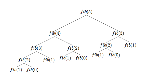
60 |
61 | The above tree represents the function calls for `fib( 5 )`
62 |
63 | Notice that when we calculate `fib( 4 )` we also calculate the value of `fib( 3 )`
64 |
65 | When we call `fib( 5 )`, it calls `fib( 3 )`, but if we already have the value of that function call from before, there's no need to recompute it.
66 |
67 | Since `fib( 5 )` asks us to call the function `fib( 3 )` _multiple times_, we have found an _overlapping subproblem_ - a subproblem that is reused numerous times, but given the same result each time it's solved.
68 |
69 | `fib( 3 )` will give us the same result no matter how many times we call it.
70 |
71 | Rather than solving these overlapping subproblems _every time_, we can do the following:
72 | - solve the subproblem once and save its value
73 | - when you need to solve the subproblem _again_, rather than going through all the computation to do the solving, return the _memorized_ value
74 |
75 | ```java
76 | int[] dp = new int[ SIZE ]; // all values initialized to 0
77 | public int fib( int n )
78 | {
79 | if ( n == 0 || n == 1 )
80 | return 1;
81 | if ( dp[ n ] != 0 )
82 | return dp[ n ];
83 | return dp[ n ] = fib( n - 1 ) + fib( n - 2 );
84 | }
85 | ```
86 |
87 | ## Pascal's Triangle
88 |
89 | In mathematics, Pascal's triangle is a triangular array of the binomial coefficients.
90 |
91 | Binomial coefficients can be read as "_n_ choose _k_" - how many ways are there to choose _k_ elements from a set of _n_ elements?
92 |
93 | The entries in each row are numbered with row _n_ = 0 at the top, and the entries in each row are numbered from the left beginning with _k_ = 0
94 |
95 | The _k__th_ element in the _n__th_ row represents "_n_ choose _k_"
96 |
97 | 
98 |
99 | Elements in each row of Pascal's triangle can be found by summing the two numbers in the row above and to the left and right of the element.
100 |
101 | This property can be seen as a closed formula:
102 |
103 | 
104 |
105 | Let's try and create a recursive method that will find us "_n_ choose _k_" using the above formula.
106 |
107 | What are the base cases?
108 |
109 | We know that there is only _one_ way to choose zero elements from an _n_-element set, as well as _one_way to choose _n_ elements from an _n_-element set.
110 |
111 | ```java
112 | // This function will return "n choose k"
113 | public int pascal( int n, int k )
114 | {
115 | if ( k == 0 || k == n )
116 | return 1;
117 | return pascal( n - 1, k - 1 ) + pascal( n - 1, k );
118 | }
119 | ```
120 |
121 | This function leaves us with the same problem we hads with the Fibonacci function: we are going to be recalculating subproblems that we have already solved before.
122 |
123 | We can fix this like we did with the Fibonacci function: memorizing the value of the subproblems so that we don't have to recalculate them later.
124 |
125 | ```java
126 | int[][] dp = new int[ N_SIZE ][ K_SIZE ];
127 | public int pascal( int n, int k )
128 | {
129 | if ( k == 0 || k == n )
130 | return 1;
131 | if ( dp[ n ][ k ] != 0 )
132 | return dp[ n ][ k ];
133 | return dp[ n ][ k ] = pascal( n - 1, k - 1 ) + pascal ( n - 1, k );
134 | }
135 | ```
136 |
137 | ## Knapsack Problem
138 |
139 | ### Problem Statement
140 |
141 | You have a knapsack that can hold up to a certain weight _W_, and you have _N_ items that you can pack for a trip; however, all of these items might not fit in your knapsack.
142 |
143 | Each item you can pack has a weight _w_ and a value _v_.
144 |
145 | Your goal is to pack some items into your knapsack such that the total weight of all of the items doesn't exceed the maximum weight limit _W_, and the sum of all the values of the items in your knapsack is _maximized_.
146 |
147 | ### Approaches
148 |
149 | 1. Calculate all subsets of items and see which subset has the highest value, but also stays under the knapsack's weight limit
150 | 2. Create some ratio for each item _v_ / _w_ and take the items with the highest ratio until you can't pack anymore
151 | 3. Use dynamic programming
152 |
153 | ### Solving Knapsack: Take I - Subset Solution
154 |
155 | Let's calculate all subsets of the _N_ items that we have.
156 |
157 | This means that there are 2_N_ possible subsets that we will need to go through.
158 |
159 | However, if _N_ is sufficiently large (larger than 25), this approach will be too slow
160 |
161 | ### Solving Knapsack: Take II - Ratio Solution
162 |
163 | Imagine we have a knapsack with _W_ = 6 and are given the following set of items:
164 | _w_ = {2, 2, 2, 5}
165 | _v_ = {7, 7, 7, 20}
166 |
167 | Let's find the _v_ / _w_ ratio of each item
168 | _v_ / _W_ = {3.5, 3.5, 3.5, 4}
169 |
170 | Now that we have the ratios, let's take the items with the greatest ratio until we have no more space left in the knapsack.
171 |
172 | We will take the item with _w_ = 5, _v_ = 20 first and put it into oiur knapsack.
173 |
174 | We now have 1 weight left in our knapsack, so we cannot fit any of the other items in our knapsack, so we end up with a value of 20.
175 |
176 | However, if we would've taken the other three items, we would've had no weight left and a value of 21 instead.
177 |
178 | ### Solving Knapsack: Take III - Dynamic Programming
179 |
180 | There are two approaches to dynamic programming:
181 | - _Top-down_: define the overall problem first and what subproblems you will need to solve in order to get your answer
182 | - _Bottom-up_: start by solving subproblems and build up to the subproblems
183 |
184 | We will look at how to solve the knapsack problem using both approaches
185 |
186 | #### Bottom-Up Solution
187 |
188 | Using the bottom-up approach, we need to first solve all of the possible subproblems, and then we can use those to solve our overall problem.
189 |
190 | We will create a table that will hold the solutions to these subproblems, and keep building on it until we are done and have our answer.
191 |
192 | Let's say we have a knapsack with capacity _W_ = 6 and the following weights and values for _N_ = 5 items:
193 | _w_ = {3, 2, 1, 4, 5}
194 | _v_ = {25, 20, 15, 40, 50}
195 |
196 | Let's figure out for all capacities, _j_, less than _W_ = 6, what is the maximum value we can get if we only use the first _i_ items
197 |
198 | `dp[ i ][ j ]` will be the solution for each subproblem
199 |
200 | Let's create our table; each cell will represent `dp[ i ][ j ]`
201 |
202 | | | | 0 | 1 | 2 | 3 | 4 | 5 | 6 |
203 | |---|---|---|---|---|---|---|---|---|
204 | | | 0 | | | | | | | |
205 | | w = 3, v = 25 | 1 | | | | | | | |
206 | | w = 2, v = 20 | 2 | | | | | | | |
207 | | w = 1, v = 15 | 3 | | | | | | | |
208 | | w = 4, v = 40 | 4 | | | | | | | |
209 | | w = 5, v = 50 | 5 | | | | | | | |
210 |
211 | If we can't use any of the items (_i_ = 0), the value at any capacity will be 0
212 |
213 | | | | 0 | 1 | 2 | 3 | 4 | 5 | 6 |
214 | |---|---|---|---|---|---|---|---|---|
215 | | | 0 | 0 | 0 | 0 | 0 | 0 | 0 | 0 |
216 | | w = 3, v = 25 | 1 | | | | | | | |
217 | | w = 2, v = 20 | 2 | | | | | | | |
218 | | w = 1, v = 15 | 3 | | | | | | | |
219 | | w = 4, v = 40 | 4 | | | | | | | |
220 | | w = 5, v = 50 | 5 | | | | | | | |
221 |
222 | For _i_ = 1, we can only take the first item in our set, so we want to take it whenever we have the capacity for it
223 |
224 | | | | 0 | 1 | 2 | 3 | 4 | 5 | 6 |
225 | |---|---|---|---|---|---|---|---|---|
226 | | | 0 | 0 | 0 | 0 | 0 | 0 | 0 | 0 |
227 | | w = 3, v = 25 | 1 | 0 | 0 | 0 | 25 | 25 | 25 | 25 |
228 | | w = 2, v = 20 | 2 | | | | | | | |
229 | | w = 1, v = 15 | 3 | | | | | | | |
230 | | w = 4, v = 40 | 4 | | | | | | | |
231 | | w = 5, v = 50 | 5 | | | | | | | |
232 |
233 | For _i_ = 2, we can now take the second item in our set in addition to the first item, but only when taking the item at a given capacity will give us greater value than not taking it.
234 |
235 | For example, at capacity _j_ = 2, previously when we didn't have the item, we could get at most 0 value, but if we now take the item, we can get at most 20 value.
236 |
237 | At capacity _j_ = 3, previously when we didn't have the item, we could get at most 25 value, but if we now take the item, we can get 20 value AND the maximum value we could get previously at capacity _j_ = 1, which is 0 (since we are looking at a capacity of _j_ = 3, and we took the second item, the capacity we have left is _j_ = 1, so we look at the maximum value we could get at this weight with all of the previous items). In this case, we do not want to take the item, because doing so will give us a lower value (20 < 25).
238 |
239 | At capacity _j_ = 5, previously when we didn't have the item, we could get at most 25 value, but if we now take the item, we can get 20 value AND the maximum value we could get previously at capacity _j_ = 3, which is 25 (since we are looking at a capacity of _j_ = 5, and we took the second item, the capacity we have left is _j_ = 3, so we look at the maximum value we could get at this weight with all of the previous items). In this case, we do want to take the item, because doing so will give us more value (45 > 25).
240 |
241 | | | | 0 | 1 | 2 | 3 | 4 | 5 | 6 |
242 | |---|---|---|---|---|---|---|---|---|
243 | | | 0 | 0 | 0 | 0 | 0 | 0 | 0 | 0 |
244 | | w = 3, v = 25 | 1 | 0 | 0 | 0 | 25 | 25 | 25 | 25 |
245 | | w = 2, v = 20 | 2 | 0 | 0 | 20 | 25 | 25 | 45 | 45 |
246 | | w = 1, v = 15 | 3 | | | | | | | |
247 | | w = 4, v = 40 | 4 | | | | | | | |
248 | | w = 5, v = 50 | 5 | | | | | | | |
249 |
250 | For _i_ = 3, we repeat the same process that we did for _i_ = 2.
251 |
252 | | | | 0 | 1 | 2 | 3 | 4 | 5 | 6 |
253 | |---|---|---|---|---|---|---|---|---|
254 | | | 0 | 0 | 0 | 0 | 0 | 0 | 0 | 0 |
255 | | w = 3, v = 25 | 1 | 0 | 0 | 0 | 25 | 25 | 25 | 25 |
256 | | w = 2, v = 20 | 2 | 0 | 0 | 20 | 25 | 25 | 25 | 25 |
257 | | w = 1, v = 15 | 3 | 0 | 15 | 20 | 35 | 40 | 45 | 60 |
258 | | w = 4, v = 40 | 4 | | | | | | | |
259 | | w = 5, v = 50 | 5 | | | | | | | |
260 |
261 | For _i_ = 4, we repeat the same process as before
262 |
263 | | | | 0 | 1 | 2 | 3 | 4 | 5 | 6 |
264 | |---|---|---|---|---|---|---|---|---|
265 | | | 0 | 0 | 0 | 0 | 0 | 0 | 0 | 0 |
266 | | w = 3, v = 25 | 1 | 0 | 0 | 0 | 25 | 25 | 25 | 25 |
267 | | w = 2, v = 20 | 2 | 0 | 0 | 20 | 25 | 25 | 45 | 45 |
268 | | w = 1, v = 15 | 3 | 0 | 15 | 20 | 35 | 40 | 45 | 60 |
269 | | w = 4, v = 40 | 4 | 0 | 15 | 20 | 35 | 40 | 55 | 60 |
270 | | w = 5, v = 50 | 5 | | | | | | | |
271 |
272 | For _i_ = 5, we repeat the same process as before
273 |
274 | | | | 0 | 1 | 2 | 3 | 4 | 5 | 6 |
275 | |---|---|---|---|---|---|---|---|---|
276 | | | 0 | 0 | 0 | 0 | 0 | 0 | 0 | 0 |
277 | | w = 3, v = 25 | 1 | 0 | 0 | 0 | 25 | 25 | 25 | 25 |
278 | | w = 2, v = 20 | 2 | 0 | 0 | 20 | 25 | 25 | 45 | 45 |
279 | | w = 1, v = 15 | 3 | 0 | 15 | 20 | 35 | 40 | 45 | 60 |
280 | | w = 4, v = 40 | 4 | 0 | 15 | 20 | 35 | 40 | 55 | 60 |
281 | | w = 5, v = 50 | 5 | 0 | 15 | 20 | 35 | 40 | 55 | 60 |
282 |
283 | Now that the table is filled out, we can solve our original problem, where _i_ = 5 and _j_ = 6, by looking up the answer from the table
284 |
285 | So our answer is: `dp[ 5 ][ 6 ]` = 60
286 |
287 | ```java
288 | for ( int i = 1; i <= N; i++ )
289 | {
290 | for ( int j = 0; j <= W; j++)
291 | {
292 | if ( weight[ i ] <= j )
293 | {
294 | if ( value[ i ] + dp[ i - 1 ][ j - weight[ i ] ] > dp[ i - 1 ][ j ] )
295 | {
296 | dp[ i ][ j ] = value[ i ] + dp[ i - 1 ][ j - weight[ i ] ];
297 | }
298 | else
299 | {
300 | dp[ i ][ j ] = dp[ i - 1 ][ j ];
301 | }
302 | }
303 | else
304 | {
305 | dp[ i ][ j ] = dp[ i - 1][ j ];
306 | }
307 | }
308 | }
309 | ```
310 |
311 | ### Top-Down Solution
312 |
313 | To solve the problem using the top-down approach, we will try to come up with some recursive function that will give us the answer.
314 |
315 | As we did with the bottom-up approach, we will go item by item and see if we want to take it or not.
316 |
317 | We will also keep track of how much weight we have left in the knapsack as we go through the items (this will help us determine if we can take an item or not).
318 |
319 | _Note_: when we're looking at an item, we only have two options: _take_ or _ignore_
320 |
321 | This is why this problem is called the "_0/1 Knapsack Problem_"
322 |
323 | ```java
324 | public int solve( int i, int j )
325 | {
326 | // Determines the max value you can get when starting at the ith item with j remaining weight left to use
327 | }
328 | ```
329 |
330 | Let's try and figure out some base cases for this function.
331 |
332 | What happens if _j_ == 0?
333 | - the max value we get by starting at _any_ index with _no weight left_ will be zero
334 |
335 | What happens if _i_ == _N_?
336 | - the max value we get by starting at an index _outside of our item range_ will be zero
337 |
338 | Let's look at every other case where _i_ != _N_ and _j_ > 0
339 |
340 | What happens if the weight of the _i__th_ item is greater than the remaining weight, _j_?
341 |
342 | If the weight of the item we are currently looking at is _greater_ than the amount of weight we have left, there's no way that we can take this item, so we _ignore_ it
343 |
344 | ```java
345 | solve( i + 1, j )
346 | ```
347 |
348 | The maximum value we get by starting at an index _where we can't take the item_ will be determined by the maximum value we get by starting at the _next_ item with the _same_ remaining weight to use.
349 |
350 | What happens if the weight of the _i__th_ item is less than or equal to the remaining weight, _j_?
351 |
352 | _Remember_, we only have two options: _take_ or _ignore_
353 |
354 | We know what ignoring an item looks like:
355 |
356 | ```java
357 | solve( i + 1, j )
358 | ```
359 |
360 | But what does _taking_ an item look like?
361 |
362 | Well, we know that the value of the remaining weight will be different
363 | - we took an item, so we need to subtract out it's weight from the remaining weight
364 |
365 | We also know that since we _took_ the item, we can add its value to our result
366 |
367 | Our resulting function call for _taking_ an item would be
368 |
369 | ```java
370 | value[ i ] + solve( i + 1, j - weight[ i ] )
371 | ```
372 |
373 | The maximum value we get by starting at an index _where we take the item_ can be determined by the sum of
374 | - the value of the item, and
375 | - the maximum value we get by starting at the _next_ item with the new remaining weight
376 |
377 | However, we just saw two separate function calls where we have enough weight to take an item, so which one do we use?
378 |
379 | ```java
380 | int ignore = solve( i + 1, j );
381 | int take = value[ i ] + solve( i + 1, j - weight[ i ] );
382 | Math.max( ignore, take );
383 | ```
384 |
385 | We now know our solution handles every case for the Knapsack problem, giving us the optimal solution when we call `solve( 0, W )`, and it shows the problem has an _optimal substructure_ - that is, an optimal solution can be constructed from the optimal solutions of its subproblems.
386 |
387 | If we solve any subproblem `solve( i, j )`, we are _guaranteed_ to get the optimal answer, and we can use these optimal subproblems to solve _other_ subproblems.
388 |
389 | We know that the problem has optimal substructure, but does it have any _overlapping subproblems_?
390 |
391 | Let's look at an example:
392 | _v_ = {100, 70, 50, 10}
393 | _w_ = {10, 4, 6, 12}
394 | _W_ = 12
395 |
396 | Imagine that we take the first item and ignore the next two
397 | - we will be at `solve( i = 3, j = 2 )`
398 |
399 | Imagine that we ignore the first item and take the next two
400 | - we will be at `solve( i = 3, j = 2 )`
401 |
402 | We have now determined we have _overlapping subproblems_, so we can save the value of a specific _index_ / _remaining weight_ pair, so we don't have to recompute the solution to the subproblem each time
403 |
404 | ```java
405 | int[][] dp = new int[ N ][ W ];
406 | public int solve( int i, int j )
407 | {
408 | // If there's no more space or we run out of items, we can't get anymore value
409 | if ( j == 0 || n == N )
410 | return 0;
411 | // If we have already solved this subproblem, return the value
412 | if ( dp[ i ][ j ] != 0 )
413 | return dp[ i ][ j ];
414 |
415 | // If the weight of the current item is greater than the weight we have left in the knapsack, ignore it
416 | if ( weight[ i ] > j )
417 | return solve( i + 1, j );
418 |
419 | // For every other case, determine if ignoring or taking the current item will yield more value
420 | int ignore = solve( i + 1, j );
421 | int take = value[ i ] + solve( i + 1, j - weight[ i ] );
422 | return dp[ i ][ j ] = Math.max( ignore, take );
423 | }
424 | ```
425 |
426 | ## Problems
427 |
428 | - [The Knapsack Problem](http://www.spoj.com/problems/KNAPSACK/)
429 | - [Party Schedule](http://www.spoj.com/problems/PARTY/)
430 | - [Tri graphs](http://www.spoj.com/problems/ACPC10D/)
431 | - [Bytelandian gold coins](http://www.spoj.com/problems/COINS/)
432 | - [Coins Game](http://www.spoj.com/problems/MCOINS/)
433 | - [Feline Olympics - Mouseball](http://www.spoj.com/problems/MBALL/)
434 | - [Piggy-Bank](http://www.spoj.com/problems/PIGBANK/)
435 | - [Mixtures](http://www.spoj.com/problems/MIXTURES/)
436 | - [TV game](https://uva.onlinejudge.org/index.php?option=com_onlinejudge&Itemid=8&page=show_problem&problem=851)
437 | - [Fire! Fire!! Fire!!!](https://uva.onlinejudge.org/index.php?option=com_onlinejudge&Itemid=8&page=show_problem&problem=1184)
438 | - [Sweet and Sour Rock](http://www.spoj.com/problems/ROCK/)
439 | - [Rent your airplane and make money](http://www.spoj.com/problems/RENT/)
440 | - [Scuba diver](http://www.spoj.com/problems/SCUBADIV/)
441 | - [ACM (ACronymMaker)](http://www.spoj.com/problems/ACMAKER/)
442 | - [Two Ends](http://www.spoj.com/problems/TWENDS/)
443 |
--------------------------------------------------------------------------------
/graph-theory/introduction/introduction.md:
--------------------------------------------------------------------------------
1 | # Graph Theory
2 |
3 | ## What is a Graph?
4 |
5 | A _graph_ consists of _vertices_ (or nodes) and _edges_ (or paths)
6 |
7 | Edges
8 | - are connections between vertices
9 | - _e.g._, roads between cities
10 | - can have one-way direction or can be bidirectional
11 | - can have weights
12 | - _e.g._, time to travel between two cities
13 |
14 | A _directional graph_ has edges that are all directional (_i.e._, if there's an edge from _A_ to _B_, there might not be one from _B_ to _A_)
15 |
16 | An _acyclic graph_ contains no cycles (in a directed graph, there's no path starting from some vertex _v_ that will take you back to _v_)
17 |
18 | A _weighted graph_ contains edges that hold a numerical value (_e.g._, cost, time, etc.)
19 |
20 | ### Unweighted, undirected graph
21 |
22 | 
23 |
24 | ### Unweighted, directed cyclic graph
25 |
26 | 
27 |
28 | ### Unweighted, directed acyclic graph
29 |
30 | 
31 |
32 | ### Weighted, undirected graph
33 |
34 | 
35 |
36 | ### Complete graph
37 |
38 | A _complete graph_ is a graph where each vertex has an edge to all other vertices in the graph
39 |
40 | 
41 |
42 | ## Representing a Graph
43 |
44 | There are two main ways to represent a graph:
45 | 1. _Adjacency matrix_
46 | 2. _Adjacency list_
47 |
48 | ### Adjacency Matrix
49 |
50 | An adjacency matrix uses a 2-dimensional array to represent edges between two vertices
51 |
52 | There are many ways to use an adjacency matrix to represent a matrix, but we will look at two variations
53 |
54 | #### Connection matrix
55 |
56 | 
57 |
58 | #### Cost matrix
59 |
60 | 
61 |
62 | #### Pros and Cons
63 |
64 | _Pros_
65 | - Easy to check if there is an edge between _i_ and _j_
66 | - calling `matrix[ i ][ j ]` will tell us if there is a connection
67 |
68 | _Cons_
69 | - To find all neighbors of vertex _i_, you would need to check the value of `matrix[ i ][ j ]` for all _j_
70 | - Need to construct a 2-dimensional array of size _N_ x _N_
71 |
72 | ### Adjacency List
73 |
74 | Rather than making space for all _N_ x _N_ possible edge connections, an _adjacency list_ keeps track of the vertices that a vertex has an edge to.
75 |
76 | We are able to do this by creating an array that contains `ArrayLists` holding the values of the vertices that a vertex is connected to.
77 |
78 | 
79 |
80 | #### Pros and Cons
81 |
82 | _Pros_
83 | - Saves memory by only keeping track of edges that a vertex has
84 | - Efficient to iterate over the edges of a vertex
85 | - Doesn't need to go through all _N_ vertices and check if there is a connection
86 |
87 | _Cons_
88 | - Difficult to quickly determine if there is an edge between two vertices
89 |
90 | ## Trees
91 |
92 | A _tree_ is a special kind of graph that exhibits the following properties:
93 | 1. Acyclic graph
94 | 2. _N_ vertices with _N_-1 edges
95 |
96 | The graphs above that we used for BFS and DFS were both trees.
97 |
98 | 
99 |
100 | Above is another example of a tree.
101 |
102 | ## Problems
103 |
104 | - [Is it a tree](http://www.spoj.com/problems/PT07Y/)
105 | - [Bitmap](http://www.spoj.com/problems/BITMAP/)
106 | - [VALIDATE THE MAZE](http://www.spoj.com/problems/MAKEMAZE/)
107 | - [Meeting For Party](http://www.spoj.com/problems/DCEPC706/)
108 | - [Slick](http://www.spoj.com/problems/UCV2013H/)
109 | - [Escape from Jail Again](http://www.spoj.com/problems/ESCJAILA/)
110 | - [A Bug's Life](http://www.spoj.com/problems/BUGLIFE/)
111 | - [Longest path in a tree](http://www.spoj.com/problems/PT07Z/)
112 | - [Treeramids](http://www.spoj.com/problems/PYRA/)
113 | - [Lucius Dungeon](http://www.spoj.com/problems/BYTESE1/)
114 | - [Mountain Walking](http://www.spoj.com/problems/MTWALK/)
115 |
--------------------------------------------------------------------------------
/graph-theory/shortest-path/dijkstras-algorithm/dijkstras-algorithm.md:
--------------------------------------------------------------------------------
1 | # Dijkstra's Algorithm
2 |
3 | ## Motivating Problem
4 |
5 | Imagine that we have a graph of flights across the country, and each flight has a given cost and time.
6 |
7 | We want to find a series of flights from city _A_ to city _B_ such that the cost (or time) is minimized.
8 |
9 | We can generalize this problem to the following:
10 |
11 | Given a graph _G_ and a starting vertex _s_, what is the _shortest path_ from _s_ to any other vertex of _G_?
12 |
13 | This problem is called the _Single-Source Shortest Paths_ (SSSP) problem.
14 |
15 | ## Single-Source Shortest Path
16 |
17 | #### SSSP on an unweighted graph
18 |
19 | If the graph is unweighted (or if all of the edges have equal or constant weight), we can use the BFS algorithm in order to solve this problem.
20 |
21 | BFS goes "level-by-level", so it would visit all vertices that are one unit away first, and then two units away, and then three units away, etc.
22 |
23 | The fact that BFS visits vertices of a graph "level-by-level" from a source vertex turns BFS into a natural choice to solve the SSSP problem on unweighted graphs.
24 |
25 | ### SSSP on a weighted graph
26 |
27 | If the given graph is weighted, BFS no longer works. This is because there can be "longer" paths from the source to vertex, but has a smaller cost than the "shorter" path found by BFS.
28 |
29 | To solve the SSSP problem on weighted graphs, we use a greedy algorithm: _Dijkstra's Algorithm_
30 |
31 | ## Dijkstra's Algorithm
32 |
33 | ### Procedure
34 |
35 | 1. Give every vertex a tentative distance
36 | - the initial vertex will have a distance of zero
37 | - every other vertex will have a distance of infinity
38 | 2. Set the initial vertex as the current vertex; mark all other vertices unvisited
39 | 3. For the current vertex, consider all of its unvisited neighbors and calculate the tentative distance to each vertex; compare the newly calculated distance to the current assigned value and set the tentative distance to the smaller distance
40 | 4. When we are done considering all of the neighbors of the current vertex, mark the current vertex as visited
41 | 5. If the destination vertex has been marked visit, or if the smallest tentative distance among unvisited vertices is infinity, stop the algorithm
42 | 6. Select the unvisited vertex that is marked with the smallest tentative distance, and set it as the new current vertex, then go back to step 3
43 |
44 | 
45 |
46 | Above is a visual representation of Dijkstra's Algorithm
47 |
48 | ### Coding Dijkstra's Algorithm
49 |
50 | There are several ways to implement this algorithm
51 | - `int[] distance`
52 | - `PriorityQueue`
53 |
54 | #### Using an array
55 |
56 | 
57 |
58 | #### Using a priority queue
59 |
60 | Remember that as you add items to a priority queue, they are automatically sorted within the queue, so that you are given the "smallest" item when you remove it from the queue.
61 |
62 | First, we need to define our `Vertex` class and what attributes it will contain.
63 |
64 | 
65 |
66 | Remember that when we used `dist[]` to keep track of distances, we had to look through _all_ tentative distances to see which vertex to visit; with this method, we just remove the next vertex from the priority queue and it will be guaranteed to have the smallest distance.
67 |
68 | Now that we have our `Vertex` class setup, how do we use it to implement Dijkstra's algorithm?
69 |
70 | Let's start by creating all of the vertices of a graph and storing them into an array.
71 |
72 | ```java
73 | Vertex[] graph = new Vertex[ N ];
74 |
75 | // For each vertex in the graph...
76 | for ( int i = 0; i < N; i++ )
77 | {
78 | // Initialize the Vertex object corresponding to the vertex
79 | graph[ i ] = new Vertex( i );
80 | }
81 |
82 | graph[ i ].neighbors.add( j ); // Add vertex j as a neighbor of vertex i
83 | ```
84 |
85 | We know the tentative distance of our source vertex is zero, so we can assign that value and add the vertex to the priority queue.
86 |
87 | ```java
88 | vertex[ source ].dist = 0;
89 | priorityQueue.add( vertex[ source ] );
90 | ```
91 |
92 | Just like BFS, we are repeating the steps of the algorithm until the queue is empty. This makes sense for Dijkstra's algorithm since we want to keep repeating the process until we either
93 | - run out of vertices (queue is empty), or
94 | - reach our destination vertex
95 |
96 | Now that we have our stopping condition, we can implement the rest of the algorithm
97 |
98 | 
99 |
100 | ## Problems
101 |
102 | - [106 miles to Chicago](http://www.spoj.com/problems/CHICAGO/)
103 | - [Highways](http://www.spoj.com/problems/HIGHWAYS/)
104 | - [Mice and Maze](http://www.spoj.com/problems/MICEMAZE/)
105 | - [ABC Path](http://www.spoj.com/problems/ABCPATH/)
106 | - [COSTLY CHESS](http://www.spoj.com/problems/CCHESS/)
107 | - [Shopping](http://www.spoj.com/problems/SHOP/)
108 | - [Prime Path](http://www.spoj.com/problems/PPATH/)
109 | - [The Benefactor](http://www.spoj.com/problems/BENEFACT/)
110 | - [Fishmonger](http://www.spoj.com/problems/FISHER/)
111 | - [Fool the Police](http://www.spoj.com/problems/FPOLICE/)
112 | - [Electric Car Rally](http://www.spoj.com/problems/CARRALLY/)
113 |
--------------------------------------------------------------------------------
/graph-theory/traversal/breadth-first-search/BreadthFirstSearch.java:
--------------------------------------------------------------------------------
1 | import java.util.*;
2 |
3 | class BreadthFirstSearch {
4 | public static void BFS(ArrayList> graph, int vertices, int root) {
5 | // visited keeps track of which nodes we have already visited
6 | boolean[] visited = new boolean[vertices + 1];
7 | // queue will keep track of which nodes we are visiting next
8 | Queue queue = new LinkedList();
9 | // add the root node to the queue and mark it as visited
10 | queue.add(root);
11 | visited[root] = true;
12 |
13 | // while the queue is not empty, continue to search the graph
14 | while (!queue.isEmpty()) {
15 | // current keeps track of the node we are currently on
16 | int current = queue.remove();
17 | // neighbors give us a list of adjacent nodes
18 | List neighbors = graph.get(current);
19 |
20 | // iterate over the neighbors and see if we have visited the node, and if not, add it to the queue
21 | for (Integer neighbor : neighbors) {
22 | // if we haven't visited the neighbor, mark it as visited and add it to the queue
23 | if (!visited[neighbor]) {
24 | visited[neighbor] = true;
25 | queue.add(neighbor);
26 | }
27 | }
28 | }
29 | }
30 | }
--------------------------------------------------------------------------------
/graph-theory/traversal/breadth-first-search/breadth-first-search.md:
--------------------------------------------------------------------------------
1 | ## Breadth-first Search
2 |
3 | _Breadth-first search_ (or BFS) is a form of graph traversal that starts at some vertex _i_ and visits all of _i_'s neighbors. It then visits all of the neighbors of _i_'s neighbors. This process keeps going until there are no more vertices left to visit.
4 |
5 | 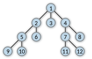
6 |
7 | Imagine a "family tree", like one shown in the picture above. BFS will visit all vertices of the same level before moving on to the next level.
8 |
9 | We start by visiting vertex 1.
10 |
11 | Then, we visit all of 1's neighbors: 2, 3, 4
12 |
13 | Then, we visit all of 1's neighbors' neighbors: 5, 6, 7, 8
14 |
15 | Finally, we visit all of their neighbors: 9, 10, 11, 12
16 |
17 | 
18 |
19 | Above is another visual representation of the BFS process starting from the top vertex.
20 |
21 | ### Coding BFS
22 |
23 | We need to use some data structure that will allow us to visit vertices "_level-by-level_", that is, visit every vertex at level _j_ before we visit any vertex at level _j_+1.
24 |
25 | In order to do this, we will be using a _Queue_ since it follows the "_first in, first out_" ordering; this means if we put all the vertices at level _j_ into the queue before the vertices at level _j_+1, we are guaranteed to visit the lower level vertices first.
26 |
27 | Below are the steps to follow for BFS:
28 | 1. Push the root vertex onto the queue
29 | 2. Pop the queue to get the current vertex
30 | 3. For each unvisited neighbor of the current vertex, mark them as visited and push them onto the queue
31 | 4. Go back to step 2 until the queue is empty
32 |
33 | ```java
34 | // Initialize the queue
35 | Queue queue = new LinkedList();
36 |
37 | // This array will tell us if we have visited a vertex
38 | boolean[] visited = new boolean[ N ];
39 |
40 | // Push the root vertex onto the queue
41 | queue.add( rootVertex );
42 |
43 | // While there is a vertex still in the queue...
44 | while ( !queue.isEmpty() )
45 | {
46 | // Get the current vertex
47 | Integer current = queue.remove();
48 | // Get the current vertex's neighbors
49 | ArrayList neighbors = graph[ current ];
50 |
51 | // For each of the current vertex's neighbors...
52 | foreach ( Integer neighbor : neighbors )
53 | {
54 | // If we haven't visited the neighbor...
55 | if ( !visited[ neighbor ] )
56 | {
57 | // Add the neighbor to the queue
58 | queue.add( neighbor );
59 | // Mark the neighbor as visited
60 | visited[ neighbor ] = true;
61 | }
62 | }
63 | }
64 | ```
--------------------------------------------------------------------------------
/graph-theory/traversal/depth-first-search/DepthFirstSearch.java:
--------------------------------------------------------------------------------
1 | import java.util.*;
2 |
3 | class DepthFirstSearch {
4 | public static void BFS(ArrayList> graph, int vertices, int root) {
5 | // visited keeps track of which nodes we have already visited
6 | boolean[] visited = new boolean[vertices + 1];
7 | // stack will keep track of which nodes we are visiting next
8 | Stack stack = new Stack();
9 | // add the root node to the stack and mark it as visited
10 | stack.push(root);
11 | visited[root] = true;
12 |
13 | // while the stack is not empty, continue to search the graph
14 | while (!stack.isEmpty()) {
15 | // current keeps track of the node we are currently on
16 | int current = stack.pop();
17 | // neighbors give us a list of adjacent nodes
18 | List neighbors = graph.get(current);
19 |
20 | // iterate over the neighbors and see if we have visited the node, and if not, add it to the stack
21 | for (Integer neighbor : neighbors) {
22 | // if we haven't visited the neighbor, mark it as visited and add it to the stack
23 | if (!visited[neighbor]) {
24 | visited[neighbor] = true;
25 | stack.push(neighbor);
26 | }
27 | }
28 | }
29 | }
30 | }
--------------------------------------------------------------------------------
/graph-theory/traversal/depth-first-search/depth-first-search.md:
--------------------------------------------------------------------------------
1 | ## Depth-first Search
2 |
3 | _Depth-first search_ (or DFS) is another form of graph traversal, but rather than visiting vertices "_level-by-level_", DFS aims to go as deep as possible in the graph before backtracking.
4 |
5 | 
6 |
7 | Imagine a "family tree", like one shown in the picture above. DFS will go as deep as it can in the graph before backtracking and repeating this process.
8 |
9 | Starting at vertex 1, the graph will travel down the left side of the graph until it hits vertex 4, where it can no longer visit any unvisited vertices.
10 |
11 | From vertex 4, it backtrack to vertex 3 and visits vertex 5, and since it can no longer visit any unvisited vertices, it backtracks to vertex 2, where it visits vertex 6.
12 |
13 | This process repeats until the entire graph has been traversed.
14 |
15 | 
16 |
17 | Above is another visual representation of the DFS process starting from the top vertex.
18 |
19 | ### Coding DFS
20 |
21 | The algorithm for DFS is very similar to that of BFS, except instead of using a _Queue_, we will be using a _Stack_.
22 |
23 | Since a _Stack_ follows the "_last in, first out_" ordering, when we are adding neighbors of a vertex to the _Stack_, the last one we push will be the next one we visit, allowing us to constantly go deeper into the graph rather than traversing level-by-level.
24 |
25 | ```java
26 | // Initialize the stack
27 | Stack stack = new Stack();
28 |
29 | // This array will tell us if we have visited a vertex
30 | boolean[] visited = new boolean[ N ];
31 |
32 | // Push the root vertex onto the stack
33 | stack.push( rootVertex );
34 |
35 | // While there is a vertex still in the stack...
36 | while ( !stack.isEmpty() )
37 | {
38 | // Get the current vertex
39 | Integer current = stack.pop();
40 | // Get the current vertex's neighbors
41 | ArrayList neighbors = graph[ current ];
42 |
43 | // For each of the current vertex's neighbors...
44 | foreach ( Integer neighbor : neighbors )
45 | {
46 | // If we haven't visited the neighbor...
47 | if ( !visited[ neighbor ] )
48 | {
49 | // Add the neighbor to the stack
50 | stack.push( neighbor );
51 | // Mark the neighbor as visited
52 | visited[ neighbor ] = true;
53 | }
54 | }
55 | }
56 | ```
--------------------------------------------------------------------------------
/problem-solving/problem-solving.md:
--------------------------------------------------------------------------------
1 | # Problem Solving
2 |
3 | ## What is problem solving?
4 |
5 | Problem solving is the ability to reach a solution for a defined problem by, potentially, using mathematical or systematic operations (algorithms).
6 |
7 | Not only an important skill to have in competitive programming, but also in the real world where problems arise everyday at jobs; being able to attack a problem quickly and efficiently is a skill desired by all companies.
8 |
9 | The following steps should serve as a general timeline for solving a problem:
10 | 1. Define the problem
11 | 2. Come up with all possible cases
12 | 3. Implement the solution
13 |
14 | In competitive programming, having a strong problem solving ability is just as important as having a strong programming background.
15 | - Even if you’ve been programming your entire life, if you don’t know how to attack a problem, coding isn’t going to help you
16 |
17 | Being able to identify edge cases and worst case scenarios for a problem are also important in competitive programming.
18 | - If you just rely on the input/output given to you in the problem statement, your code might not handle ALL cases (which is necessary for an accepted solution)
19 |
20 | ## How do we break a problem down?
21 |
22 | If we are given a problem to work on, what are the steps we must take in order to get an accepted solution? Here are the basic steps to follow:
23 |
24 | 1. Read the problem
25 | 2. Manually solve the problem
26 | 3. Take note of the constraints
27 | 4. Implement a solution
28 | 5. Optimize your solution
29 | 6. Handle edge cases
30 |
31 | ### Step 1: Read the problem
32 |
33 | Yes, this is an obvious step in solving a problem, but it is a step that can cause turmoil in the long run.
34 |
35 | Even if the background story behind a problem is silly or boring, you must read the problem all the way through to make sure that you didn’t miss any important details that are critical to solving the problem.
36 |
37 | If you spent 45 minutes solving a problem with some algorithm, but realize later that the problem asked you to do something completely different, you don’t get that time back.
38 |
39 | ### Step 2: Manually solve the problem
40 |
41 | You will be given input and output for a problem, so you should take a few minutes to grab pen and paper and figure out how they got their answer.
42 |
43 | Writing out how they derived their output from the given input will give you a general algorithm for your solution; start by taking the steps you took and turning those into lines of code.
44 |
45 | This will also stop you from jumping into the problem straight away and saying “how did they get that answer?” when debugging your code down the road.
46 |
47 | ### Step 3: Take note of the constraints
48 |
49 | Step 3: Take note of the constraints
50 | These are the size of the input variables that are given to you by the problem (e.g., `X <= 1,000,000`).
51 |
52 | Knowing the sizes of the variables that are given can eliminate possible algorithms that you chose to use.
53 |
54 | In order to know what is a good algorithm for a given constraint, you will need to understand **Big O Notation**.
55 |
56 | For most problems, you can assume that your program will be able to process ~100,000,000 operations per second.
57 |
58 | Additionally, most problems will have a time limit between 0.5 and 3 seconds, so the number of "steps" your algorithm takes cannot exceed ~300M.
59 |
60 | ### Step 4: Implement a solution
61 |
62 | Use the algorithm/pseudocode you came up with when manually solving the test cases to implement a basic solution.
63 |
64 | **Remember:** this algorithm you came up with does not need to be optimal; as long as you can come up with something that will get you the correct answer, you can worry about optimizing afterwards.
65 |
66 | ### Step 5: Optimize your solution
67 |
68 | Making sure that your code can handle the constraints of the input is key to getting AC on a problem; if you don’t take this step into account, you won’t be able to get anything but **Time Limit Exceeded** on a problem.
69 |
70 | Thinks of ways to eliminate unnecessary loops and operations within your code in order to trim off some time so that you can efficiently solve the problem.
71 |
72 | ### Step 6: Handle edge cases
73 |
74 | Being able to come up with *tricky* test cases that the judge possibly came up with can save you trouble in the long run (as well as avoid a **Wrong Answer**). Here are some things to keep in mind:
75 | - Did you handle the minimum and maximum cases?
76 | - Did you handle potential negative numbers?
77 | - Is the problem using **longs** instead of **ints**?
78 | - Is there potential for your code to throw a **runtime error**? (e.g., array out of bounds, stack overflow, etc.)
79 |
80 | ## Conclusion
81 |
82 | If you followed all of the previous steps, you can go ahead and submit your solution to the judge and see if you get AC.
83 |
84 | If you happen to get **Wrong Answer**, **Time Limit Exceeded**, or **Runtime Error**, make sure that you read the problem correctly, handled all cases, have a fast enough algorithm, and that your program isn't crashing when being tested.
85 |
86 | ## Problems - Easy
87 |
88 | - [Life, the Universe, and Everything](http://www.spoj.com/problems/TEST/)
89 | - [To and Fro](http://www.spoj.com/problems/TOANDFRO/)
90 | - [Adding Reversed Numbers](http://www.spoj.com/problems/ADDREV/)
91 | - [Traversing Grid](http://www.spoj.com/problems/TRGRID/)
92 | - [Anti-Blot System](http://www.spoj.com/problems/ABSYS/)
93 | - [What's Next](http://www.spoj.com/problems/ACPC10A/)
94 | - [Alpha Centauri Tennis](http://www.spoj.com/problems/ACT/)
95 | - [Rectangles](http://www.spoj.com/problems/AE00/)
96 | - [Christmas Play](http://www.spoj.com/problems/AMR10G/)
97 | - [Complete the Series (Easy)](http://www.spoj.com/problems/AP2/)
98 | - [Simple Arithmetics II](http://www.spoj.com/problems/ARITH2/)
99 | - [Common Permutation](http://www.spoj.com/problems/CPRMT/)
100 | - [A Very Easy Problem!](http://www.spoj.com/problems/EASYPROB/)
101 | - [Pizza](http://www.spoj.com/problems/EGYPIZZA/)
102 | - [Traveling Salesman](http://www.spoj.com/problems/FAKETSP/)
103 | - [Happy Numbers I](http://www.spoj.com/problems/HPYNOS/)
104 | - [Java vs C++](http://www.spoj.com/problems/JAVAC/)
105 | - [Not a Triangle](http://www.spoj.com/problems/NOTATRI/)
106 | - [Ambiguous Permutations](http://www.spoj.com/problems/PERMUT2/)
107 |
108 | ## Problems - Medium
109 |
110 | - [Colours A, B, C, D](http://www.spoj.com/problems/ABCD/)
111 | - [Aliens at the train](http://www.spoj.com/problems/ALIEN/)
112 | - [Bye Bye Cakes](http://www.spoj.com/problems/BYECAKES/)
113 | - [The Great Ball](http://www.spoj.com/problems/BYTESE2/)
114 | - [Headshot](http://www.spoj.com/problems/HEADSHOT/)
115 | - [Hotels Along the Croatian Coast](http://www.spoj.com/problems/HOTELS/)
116 | - [Just Next !!!](http://www.spoj.com/problems/JNEXT/)
117 | - [The Next Palindrome](http://www.spoj.com/problems/PALIN/)
118 | - [Rat Attack](https://uva.onlinejudge.org/index.php?option=onlinejudge&page=show_problem&problem=1301)
119 | - [Do it Wrong, Get it Right](http://www.spoj.com/problems/DWRONG/)
120 |
121 | ## Problems - Hard
122 |
123 | - [Hexagram](http://www.spoj.com/problems/HEXGRAM/)
124 | - [Mickey Mouse Magic Trick v3](http://www.spoj.com/problems/MMMAGIC3/)
125 | - [Beautiful Mountains](http://www.spoj.com/problems/MOUNTAIN/)
126 | - [Nested Palindromes](http://www.spoj.com/problems/NESPALIN/)
127 | - [Shuffles](http://www.spoj.com/problems/SHUFFLES/)
128 | - [Walls](http://www.spoj.com/problems/WALLSPRO/)
129 | - [Unhappy Numbers](http://www.spoj.com/problems/UNHAPPY/)
130 |
--------------------------------------------------------------------------------
/resources/binary-search.png:
--------------------------------------------------------------------------------
https://raw.githubusercontent.com/shashishailaj/Competitive-Programming/b1a3c3c235c9b0df072f6343d78402d1dc981677/resources/binary-search.png
--------------------------------------------------------------------------------
/resources/graph-theory-dijkstras-algorithm-1.png:
--------------------------------------------------------------------------------
https://raw.githubusercontent.com/shashishailaj/Competitive-Programming/b1a3c3c235c9b0df072f6343d78402d1dc981677/resources/graph-theory-dijkstras-algorithm-1.png
--------------------------------------------------------------------------------
/resources/graph-theory-dijkstras-algorithm-2.png:
--------------------------------------------------------------------------------
https://raw.githubusercontent.com/shashishailaj/Competitive-Programming/b1a3c3c235c9b0df072f6343d78402d1dc981677/resources/graph-theory-dijkstras-algorithm-2.png
--------------------------------------------------------------------------------
/resources/graph-theory-dijkstras-algorithm-3.png:
--------------------------------------------------------------------------------
https://raw.githubusercontent.com/shashishailaj/Competitive-Programming/b1a3c3c235c9b0df072f6343d78402d1dc981677/resources/graph-theory-dijkstras-algorithm-3.png
--------------------------------------------------------------------------------
/resources/graph-theory-introduction-1.png:
--------------------------------------------------------------------------------
https://raw.githubusercontent.com/shashishailaj/Competitive-Programming/b1a3c3c235c9b0df072f6343d78402d1dc981677/resources/graph-theory-introduction-1.png
--------------------------------------------------------------------------------
/resources/graph-theory-introduction-2.png:
--------------------------------------------------------------------------------
https://raw.githubusercontent.com/shashishailaj/Competitive-Programming/b1a3c3c235c9b0df072f6343d78402d1dc981677/resources/graph-theory-introduction-2.png
--------------------------------------------------------------------------------
/resources/graph-theory-introduction-3.png:
--------------------------------------------------------------------------------
https://raw.githubusercontent.com/shashishailaj/Competitive-Programming/b1a3c3c235c9b0df072f6343d78402d1dc981677/resources/graph-theory-introduction-3.png
--------------------------------------------------------------------------------