89 |
90 |
91 |
92 |
93 | {% include _templateFolder+'scripts.html' %}
94 |
95 |
96 |
--------------------------------------------------------------------------------
/www/articles/ipython-in-teaching.md:
--------------------------------------------------------------------------------
1 | Last fall I was a part of a TA team (along with Mr. Seogi Kang!) for my supervisor's undergrad geophysics course.
2 | The course is targeted at geologists and engineers who my work with geophysicists over the course of their careers.
3 | So the aim of much of the content, labs, assignments, etc. is to equip them with the tools to communicate with geophysicsist.
4 | This year, we embarked on a fairly major overhaul. We wanted to (and are still working to) re-vamp the way much of the material was presented to make it more engaging for students.
5 | It is an interesting platform to explore how we explain concepts rooted in physics without getting bogged down in the math.
6 |
7 | It is actually pretty incredible how much information we can compress into a collection of symbols strung together to describe governing equations, but that is not the point of this course.
8 | This group of students needs enough intuition to have an idea of where geophysical techniques may be useful for the applications they may encounter in their careers and meaningful conversation with a geophysicist.
9 |
10 | Building intuition requires a place where you can ask *What if...?*, try something, and get an answer.
11 | If you ask enough *What if...?*'s, you can get a feel for the physics occurring between the input and the result.
12 | Numerical simulations are an extremely powerful tool for asking these types of questions.
13 | But how do you give students access to these tools without the having them get stuck in the overhead of coding?: You make toys!
14 |
15 | Enter the [IPython notebook](http://ipython.org/notebook.html) and the [interact widget](http://nbviewer.ipython.org/github/adrn/ipython/blob/master/examples/Interactive%20Widgets/Index.ipynb).
16 | Early in the semester, we did a lab on constructing a normal incidence seismogram.
17 | We started by having them investigate the connection between the relevant physical properties, density and seismic velocity, and the reflectivity series.
18 | What physical property combinations make the refection coefficients to be positive?, negative?, zero?
19 |
20 | 
21 |
22 | These reflection coefficients are given in depth, but a seismogram is measured in time. How do we make that translation?
23 |
24 | 
25 |
26 | When we go out and complete a seismic survey, we use a source wavelet. How do we get a seismogram? What happens if we make the input wavelet wider?
27 |
28 | 
29 |
30 | Now we have walked through each of the pieces. Lets play with the inputs: the physical property model and wavelet and see what we get out. Can you construct models where we don't see a layer? What happens if you add noise?
31 |
32 | 
33 |
34 | Check it out on github: [gpgTutorials/Seismic/SyntheticSeismogram](https://github.com/ubcgif/gpgTutorials/tree/master/Seismic/SyntheticSeismogram)
35 |
36 |
37 | ### Other reasons the notebook is a great teaching tool:
38 |
39 | - It is easy to vary the level of detail exposed to students. For this lab, we hide pretty much everything in .py files, but it is easy to break out and include pieces of code that you want students to be exposed to.
40 | - Regardless of how much you choose to show them in the notebook, the real deal is underneath. If students are curious, they can dig deeper; it is not packaged in a black-box that ends in .exe.
41 | - and... open source for the win! There are great examples and tools out there that both reduce the workload on developers and provide some great ideas for explaining a variety of concepts.
42 |
43 |
44 | ### What did the students think?
45 |
46 | At the end of the term, we asked the students for feedback on a variety of aspects of the course. Overall, we recieved repeated feedback that the IPython tools we developed were among the more valueable tools they had access to in the course. I think we can be assured that by letting them play with the concepts, we are taking a step in the right direction.
47 |
--------------------------------------------------------------------------------
/article/article.py:
--------------------------------------------------------------------------------
1 | import datetime
2 | import requests
3 | import jinja2
4 | import json
5 | import markdown
6 |
7 |
8 | KNOWN_LICENCES = {
9 | "CC-BY-4.0": """ This work is licensed under a Creative Commons Attribution 4.0 International License.""",
10 | "CC-BY-SA-4.0": """ This work is licensed under a Creative Commons Attribution-ShareAlike 4.0 International License.""",
11 | "CC-BY-NC-4.0": """ This work is licensed under a Creative Commons Attribution-NonCommercial 4.0 International License.""",
12 | "CC-BY-ND-4.0": """ This work is licensed under a Creative Commons Attribution-NoDerivatives 4.0 International License.""",
13 | "CC-BY-NC-ND-4.0": """ This work is licensed under a Creative Commons Attribution-NonCommercial-NoDerivatives 4.0 International License.""",
14 | "CC-BY-NC-SA-4.0": """ This work is licensed under a Creative Commons Attribution-NonCommercial-ShareAlike 4.0 International License.""",
15 | }
16 |
17 | contributors_dict = dict()
18 |
19 |
20 | def add_contributors(people):
21 | for k in people:
22 | contributors_dict[k] = people[k]
23 |
24 |
25 | def read_date(date_str):
26 | if len(date_str) == 10:
27 | return datetime.datetime.strptime(date_str, "%d/%m/%Y")
28 | return datetime.datetime.strptime(date_str, "%Y-%m-%dT%H:%M:%SZ")
29 |
30 |
31 | class MDArticle(object):
32 |
33 | def __init__(self, slug):
34 | with open("articles/{}.json".format(slug), "r") as f:
35 | self.meta = json.loads(f.read())
36 | with open("articles/{}.md".format(slug), "r") as f:
37 | self.content = f.read()
38 |
39 | self.contributors = self.meta["contributors"]
40 |
41 | @property
42 | def html_content(self):
43 | return markdown.markdown(self.content, extensions=[
44 | 'markdown.extensions.tables',
45 | 'markdown.extensions.fenced_code'
46 | ])
47 |
48 | @property
49 | def avatar(self):
50 | return contributors_dict[self.contributors["authors"][0]]['avatar']
51 |
52 | @property
53 | def source(self):
54 | return "https://gist.github.com/" + self.gist_id
55 |
56 | @property
57 | def date(self):
58 | return read_date(self.meta['date_published'])
59 |
60 | # HTML rendering targets
61 |
62 | @property
63 | def html_title(self):
64 | return self.meta['title']
65 |
66 | @property
67 | def html_authors(self):
68 | return contributors_dict[self.contributors["authors"][0]]['name']
69 |
70 | @property
71 | def html_content(self):
72 | return markdown.markdown(self.content, extensions=[
73 | 'markdown.extensions.tables',
74 | 'markdown.extensions.fenced_code'
75 | ])
76 |
77 | @property
78 | def html_license(self):
79 | return KNOWN_LICENCES["CC-BY-4.0"]
80 |
--------------------------------------------------------------------------------
/www/templates/why.html:
--------------------------------------------------------------------------------
1 |
2 |
3 |
4 | SimPEG
5 | {% include _templateFolder+'head.html' %}
6 |
7 |
21 |
22 |
23 | {% include _templateFolder+'navBar.html' %}
24 |
25 |
26 |
27 |
28 |
29 |
30 |
31 |
32 |
January 2015
33 |
Why SimPEG
34 |
35 |
Our essential functions as researchers are the pursuit and dissemination of knowledge through research and education. As scientists we seek to find models that reproduce the observations that we make in the world. In geophysics, we use inverse theory to mathematically create models of the earth from measured data. It is a difficult problem with many moving pieces: physics, discretization, simulation, regularization, optimization, computer science, linear algebra, geology. Exploring each of these disciplines can take a career, if you are so inclined, but as geophysicists we care about the combination: how to pull these disciplines together to answer our questions. This is the first problem we hope to help solve: to create a toolbox for the geophysicist that allows you to work at a high level and keep your geophysical question in focus. However, a toolbox is not enough. The research questions that we are interested in surround the integration of information to make better decisions.
36 |
We believe that the feedback loops in the geosciences could use some serious work. For example, collect multiple data-sets from the same field area (geology, seismic, electromagnetics, hydrogeology), process the data separately, and then reconvene with your multidisciplinary team. You may be rather surprised (or not) that the everyone has a (completely!?) different model. Dissonant at best, but often conflicting in the details. Therein lies the second problem: how do we integrate these geoscience fields? Not by force or even by default, but at least to have the option of quantitative communication and built in feedback loops. What we require is an implementation that is inherently and unequivocally modular, with all pieces available to manipulation. Black-box software, where the implementations are hidden, obfuscated, or difficult to manipulate, do not promote experimentation and investigation. We are working on a framework that exposes the details of the implementation to the geophysicist in a manner that promotes productivity and question based interrogation. This framework can be easily extended to encompass many geophysical problems and is built with the inverse problem as the fundamental goal.
37 |
The future we see is a mix of tools that span our disciplines, and a framework that allows us to integrate many different types of geophysical data so that we can communicate effectively and experiment efficiently. A toolbox combined with a framework that allows you to solve your own problems, and creates opportunities for us to work together to better image and understand the subsurface. What we are building is called SimPEG, simulation and parameter estimation in geophysics. We are building it in the open. We are testing it. Breaking it. Building it. Fixing it. Using it. If you believe, like we do, that geophysics can be more innovative and informative in the open and that these tools are necessary and invaluable in education as well as research, then you should get in touch. There is a lot of work to do!
38 |
39 |
40 |
41 |
Rowan Cockett
42 |
Lindsey Heagy
43 |
Seogi Kang
44 |
45 |
46 |
47 |
48 |
49 |
50 |
51 |
52 |
53 |
54 |
55 | {% include _templateFolder+'footer.html' %}
56 |
57 | {% include _templateFolder+'scripts.html' %}
58 |
59 |
60 |
--------------------------------------------------------------------------------
/www/css/notebook.css:
--------------------------------------------------------------------------------
1 | .highlight .hll { background-color: #ffffcc }
2 | .highlight { background: #f8f8f8; }
3 | .highlight .c { color: #408080; font-style: italic } /* Comment */
4 | .highlight .err { border: 1px solid #FF0000 } /* Error */
5 | .highlight .k { color: #008000; font-weight: bold } /* Keyword */
6 | .highlight .o { color: #666666 } /* Operator */
7 | .highlight .cm { color: #408080; font-style: italic } /* Comment.Multiline */
8 | .highlight .cp { color: #BC7A00 } /* Comment.Preproc */
9 | .highlight .c1 { color: #408080; font-style: italic } /* Comment.Single */
10 | .highlight .cs { color: #408080; font-style: italic } /* Comment.Special */
11 | .highlight .gd { color: #A00000 } /* Generic.Deleted */
12 | .highlight .ge { font-style: italic } /* Generic.Emph */
13 | .highlight .gr { color: #FF0000 } /* Generic.Error */
14 | .highlight .gh { color: #000080; font-weight: bold } /* Generic.Heading */
15 | .highlight .gi { color: #00A000 } /* Generic.Inserted */
16 | .highlight .go { color: #888888 } /* Generic.Output */
17 | .highlight .gp { color: #000080; font-weight: bold } /* Generic.Prompt */
18 | .highlight .gs { font-weight: bold } /* Generic.Strong */
19 | .highlight .gu { color: #800080; font-weight: bold } /* Generic.Subheading */
20 | .highlight .gt { color: #0044DD } /* Generic.Traceback */
21 | .highlight .kc { color: #008000; font-weight: bold } /* Keyword.Constant */
22 | .highlight .kd { color: #008000; font-weight: bold } /* Keyword.Declaration */
23 | .highlight .kn { color: #008000; font-weight: bold } /* Keyword.Namespace */
24 | .highlight .kp { color: #008000 } /* Keyword.Pseudo */
25 | .highlight .kr { color: #008000; font-weight: bold } /* Keyword.Reserved */
26 | .highlight .kt { color: #B00040 } /* Keyword.Type */
27 | .highlight .m { color: #666666 } /* Literal.Number */
28 | .highlight .s { color: #BA2121 } /* Literal.String */
29 | .highlight .na { color: #7D9029 } /* Name.Attribute */
30 | .highlight .nb { color: #008000 } /* Name.Builtin */
31 | .highlight .nc { color: #0000FF; font-weight: bold } /* Name.Class */
32 | .highlight .no { color: #880000 } /* Name.Constant */
33 | .highlight .nd { color: #AA22FF } /* Name.Decorator */
34 | .highlight .ni { color: #999999; font-weight: bold } /* Name.Entity */
35 | .highlight .ne { color: #D2413A; font-weight: bold } /* Name.Exception */
36 | .highlight .nf { color: #0000FF } /* Name.Function */
37 | .highlight .nl { color: #A0A000 } /* Name.Label */
38 | .highlight .nn { color: #0000FF; font-weight: bold } /* Name.Namespace */
39 | .highlight .nt { color: #008000; font-weight: bold } /* Name.Tag */
40 | .highlight .nv { color: #19177C } /* Name.Variable */
41 | .highlight .ow { color: #AA22FF; font-weight: bold } /* Operator.Word */
42 | .highlight .w { color: #bbbbbb } /* Text.Whitespace */
43 | .highlight .mf { color: #666666 } /* Literal.Number.Float */
44 | .highlight .mh { color: #666666 } /* Literal.Number.Hex */
45 | .highlight .mi { color: #666666 } /* Literal.Number.Integer */
46 | .highlight .mo { color: #666666 } /* Literal.Number.Oct */
47 | .highlight .sb { color: #BA2121 } /* Literal.String.Backtick */
48 | .highlight .sc { color: #BA2121 } /* Literal.String.Char */
49 | .highlight .sd { color: #BA2121; font-style: italic } /* Literal.String.Doc */
50 | .highlight .s2 { color: #BA2121 } /* Literal.String.Double */
51 | .highlight .se { color: #BB6622; font-weight: bold } /* Literal.String.Escape */
52 | .highlight .sh { color: #BA2121 } /* Literal.String.Heredoc */
53 | .highlight .si { color: #BB6688; font-weight: bold } /* Literal.String.Interpol */
54 | .highlight .sx { color: #008000 } /* Literal.String.Other */
55 | .highlight .sr { color: #BB6688 } /* Literal.String.Regex */
56 | .highlight .s1 { color: #BA2121 } /* Literal.String.Single */
57 | .highlight .ss { color: #19177C } /* Literal.String.Symbol */
58 | .highlight .bp { color: #008000 } /* Name.Builtin.Pseudo */
59 | .highlight .vc { color: #19177C } /* Name.Variable.Class */
60 | .highlight .vg { color: #19177C } /* Name.Variable.Global */
61 | .highlight .vi { color: #19177C } /* Name.Variable.Instance */
62 | .highlight .il { color: #666666 } /* Literal.Number.Integer.Long */
63 |
64 |
65 |
66 |
67 | div.prompt{width:11ex;padding:0.4em;margin:0px;font-family:monospace;text-align:right;line-height:1.231em;}
68 | div.input_prompt{color:navy;border-top:1px solid transparent;}
69 | div.out_prompt_overlay{height:100%;padding:0px 0.4em;position:absolute;border-radius:4px;}
70 | div.out_prompt_overlay:hover{-webkit-box-shadow:inset 0 0 1px #000000;-moz-box-shadow:inset 0 0 1px #000000;box-shadow:inset 0 0 1px #000000;background:rgba(240, 240, 240, 0.5);}
71 | div.output_prompt{color:darkred;}
72 | div.output_area{padding:0px;page-break-inside:avoid;display:-webkit-box;-webkit-box-orient:horizontal;-webkit-box-align:stretch;display:-moz-box;-moz-box-orient:horizontal;-moz-box-align:stretch;display:box;box-orient:horizontal;box-align:stretch;}
73 | div.output_area pre{font-family:monospace;margin:0;padding:0;border:0;font-size:100%;vertical-align:baseline;color:black;background-color:transparent;-webkit-border-radius:0;-moz-border-radius:0;border-radius:0;line-height:inherit;}
74 | div.output_subarea{padding:0.44em 0.4em 0.4em 1px;margin-left:6px;-webkit-box-flex:1;-moz-box-flex:1;box-flex:1;}
75 | div.output_text{text-align:left;color:#000000;font-family:monospace;line-height:1.231em;}
76 | div.output_stream{padding-top:0.0em;padding-bottom:0.0em;}
77 | div.output_stderr{background:#fdd;}
78 | div.output_latex{text-align:left;}
79 | img{max-width:100%;width:auto\9;height:auto;vertical-align:middle;border:0;-ms-interpolation-mode:bicubic;}
80 |
81 | div.prompt{display: none;}
82 | div.output_html{text-align: center;}
83 |
84 |
--------------------------------------------------------------------------------
/www/articles/nudging-geophysics.md:
--------------------------------------------------------------------------------
1 | The goal of geophysical inversions is to image the subsurface of the earth (without digging anything up!!).
2 | The realization of this goal can be hard because it requires a deep understanding in several disciplines
3 | including geology, physics, math, and computer science. Due to the diversity required to complete an inversion,
4 | geophysical researchers are susceptible to get 'lost' on their way to realizing their **geophysical ideas**.
5 | Researchers are always having new ideas; however, most of them are not realized in the world, because of the
6 | difficulties in communication among many disciplines in an organized way.
7 |
8 | Ideas are fickle and, in my experience, only stick with you for a short amount of time with any sort of clarity.
9 | Ideas need to be incubated in the proper environment if they are to be realized in the world. The motivation behind
10 | SimPEG (Simulation and Parameter Estimation in Geophysics) is to provide a toolbox and a framework such that
11 | geophysical researchers can realize their ideas quickly and efficiently. In this way we hope that researchers
12 | won't lose the momentum of their geophysical curiosity and perhaps realize a few more ideas!
13 |
14 | 
15 |
16 | In order to show some of the capabilities of SimPEG we will show an example of simulating physics, which is a
17 | fundamental step in any geophysical inversion. Sometimes, geophysicists go to the field and hook up a battery
18 | to the ground. They then use a voltmeter to measure the response from the earth on the ground surface.
19 |
20 | 
21 |
22 | This geophysical survey called a direct current (DC) resistivity survey, and it is one of the most used
23 | geophysical methods in environmental engineering and the mining industry. Amazingly, with the proper application
24 | of geophysical inversions to the measured DC resistivity data, we can restore the resistivity distribution and
25 | image the subsurface of the earth. In this example, we simulate the physics in DC resistivity survey, and show
26 | how different disciplines including math, physics and computer science can be connected intuitively through
27 | SimPEG's toolbox.
28 |
29 | ## Example: DC resistivity survey
30 |
31 | ```python
32 | from SimPEG import Mesh, Utils, Solver
33 | import scipy
34 | %pylab inline
35 | ```
36 |
37 | ### Bring the earth into your computer and represent it as numbers: discretization (mesh)
38 |
39 | ```python
40 | cs = 5
41 | hx = np.ones(250)*cs
42 | hy = np.ones(250)*cs
43 | mesh = Mesh.TensorMesh([hx, hy], 'C0')
44 | m = Mesh.TensorMesh([10, 10], 'CC')
45 | fig, ax = plt.subplots(1,1, figsize = (5,5))
46 | m.plotGrid(nodes=True, faces=True, centers=True, ax = ax)
47 | ax.legend(('nodes', 'cell-center', 'x-face', 'y-face'), loc=1)
48 | ```
49 |
50 | 
51 |
52 | ### Discipline #1: Maxwell's quations in steady state (Physics)
53 |
54 | $$
55 | \nabla \cdot \sigma \nabla \phi = -q
56 | $$
57 |
58 | ### Discipline #2: In discretized space (Finite volume Discretization)
59 |
60 | $$
61 | \mathbf{A} = \mathbf{Div} \mathbf{diag}(\mathbf{Av}_{cc}^{F T}\mathbf{\sigma})\mathbf{Grad} \\
62 | \mathbf{A}\phi = -\mathbf{q}
63 | $$
64 |
65 | ### Discipline #3: Code
66 |
67 | ```python
68 | Div = mesh.faceDiv
69 | Grad = mesh.cellGrad
70 | vol = mesh.vol
71 | AvF2CC = mesh.aveF2CC
72 | sigma = np.ones(mesh.nC)*1e-2
73 | getA = lambda sigma: Div*(Utils.sdiag(AvF2CC.T*sigma))*Grad
74 | A = getA(sigma)
75 | q = np.zeros(mesh.nC)
76 | inds = Utils.closestPoints(mesh,[[-400, 1200],[400,1200]])
77 | q[inds] = [-1., +1]
78 | ```
79 |
80 | Those three different disciplines including physics, math (discretization) and computer science (code) can be
81 | intuitively connected through SimPEG's toolbox. In my experience, this is awesome to test your rough ideas really fast.
82 |
83 |
84 | ## Compute responses for homogeneous earth
85 |
86 | ```python
87 | phi_half = Solver(A)*-q
88 | fig, ax = plt.subplots(1,1, figsize=(10,7))
89 | dat = mesh.plotImage(Grad*(phi_half), vType='F', view = 'vec', streamOpts={'color': 'w'}, ax=ax)
90 | cb = plt.colorbar(dat[0])
91 | cb.set_label('Electric field (V/m)', fontsize=14)
92 | ```
93 |
94 | 
95 |
96 |
97 | ## Compute responses for *heterogeneous* earth
98 |
99 | Perhaps from a python embedded in a resistive circle?
100 |
101 | ```python
102 | img = scipy.misc.imread('SciPy_2014.png')
103 | sigma_scipy = Utils.mkvc(img[:,:,0].astype(float))*1e-2 + 1e-2
104 | fig, ax = plt.subplots(1,1, figsize=(10,7))
105 | dat = mesh.plotImage(sigma_scipy,ax=ax)
106 | cb = plt.colorbar(dat[0])
107 | cb.set_label('Conductivity (S/m)', fontsize=14)
108 | ```
109 |
110 | 
111 |
112 | ```python
113 | A = getA(sigma_scipy)
114 | phi_scipy = Solver(A) * -q
115 | fig, ax = plt.subplots(1,1, figsize=(10,7))
116 | # dat = mesh.plotImage(phi, ax=ax)
117 | dat = mesh.plotImage(Grad*(phi_scipy), vType='F', view = 'vec', streamOpts={'color': 'w'}, ax=ax)
118 | cb = plt.colorbar(dat[0])
119 | cb.set_label('Electric field (V/m)', fontsize=14)
120 | ```
121 |
122 | 
123 |
124 | Look some distortions in the electric field of the earth due to a python! By measuring this perturbed electric
125 | fields on the surface, we can potentially recover conductivity distribution of the earth. Doing a geophysical
126 | inversion is still a bit more work (maybe for the next blog article?), but simulating the fields is a crucial
127 | first step! The goal of SimPEG is that you can move fast, and the process is interactive so you can get rapid
128 | feedback on your ideas. There might not actually be pythons is the subsurface, but it is good that it doesn't
129 | take too long to check...!
130 |
131 | This article is written for 2014 AGU Fall Meeting.
132 |
--------------------------------------------------------------------------------
/www/simpeg.py:
--------------------------------------------------------------------------------
1 |
2 | import os
3 | import sys
4 |
5 | sys.path.insert(1, os.path.join(os.path.abspath('.'), 'lib'))
6 |
7 | import datetime
8 | import webapp2
9 |
10 | from google.appengine.ext import ndb
11 | from google.appengine.api import users
12 | from google.appengine.api import mail
13 | from google.appengine.api import urlfetch
14 |
15 | import jinja2
16 | import urllib
17 | import hashlib
18 | import json
19 | import markdown
20 |
21 | import requests
22 | from requests_toolbelt.adapters import appengine
23 | appengine.monkeypatch()
24 |
25 | from article import MDArticle, add_contributors
26 |
27 |
28 | with open("contributors.json", "r") as f:
29 | add_contributors(json.loads(f.read()))
30 |
31 |
32 | SLUGS = [
33 | "primary-secondary-approaches",
34 | "inversions-of-airborne-tdem",
35 | "a-first-peak-into-the-black-box",
36 | "implementations-of-fdem",
37 | "ipython-in-teaching",
38 | "moving-between-dimensions",
39 | "exploring-julia",
40 | "nudging-geophysics",
41 | "scipy2014"
42 | ]
43 |
44 | ARTICLES = []
45 | for slug in SLUGS:
46 | with open("articles/{}.json".format(slug), "r") as f:
47 | ARTICLES += [json.loads(f.read())]
48 |
49 |
50 | JINJA_ENVIRONMENT = jinja2.Environment(
51 | loader=jinja2.FileSystemLoader(
52 | os.path.join(os.path.dirname(__file__).split('/')[:-1])),
53 | extensions=['jinja2.ext.autoescape'],
54 | autoescape=False
55 | )
56 |
57 |
58 | def setTemplate(self, template_values, templateFile):
59 | _templateFolder = 'templates/'
60 | # add Defaults
61 | template_values['_templateFolder'] = _templateFolder
62 | template_values['_year'] = str(datetime.datetime.now().year)
63 |
64 | path = os.path.normpath(_templateFolder+templateFile)
65 | template = JINJA_ENVIRONMENT.get_template(path)
66 | self.response.write(template.render(template_values))
67 |
68 |
69 | class MainPage(webapp2.RequestHandler):
70 |
71 | def get(self):
72 | packages = [
73 | dict(name="SimPEG", link="simpeg", status="check",
74 | color="green",
75 | description="A framework for simulation and gradient based parameter estimation in geophysics."),
76 | dict(name="simpegEM", link="simpeg", status="check",
77 | color="green",
78 | description="A electromagnetic forward modeling and inversion package for SimPEG."),
79 | dict(name="simpegNSEM", link="simpeg", status="refresh",
80 | color="green",
81 | description="Magnetotellurics forward and inverse codes for SimPEG"),
82 | dict(name="simpegDC", link="simpeg", status="refresh",
83 | color="orange",
84 | description="A DC resistivity forward modelling and inversion package for SimPEG."),
85 | dict(name="simpegPF", link="simpeg", status="refresh",
86 | color="orange",
87 | description="Potential fields codes for SimPEG. Gravity and Magnetics."),
88 | dict(name="simpegFLOW", link="simpeg", status="flask",
89 | color="orange",
90 | description="Groundwater (vadose zone) flow equations written in the SimPEG framework."),
91 | dict(name="simpegSEIS", link="simpegseis", status="wrench",
92 | color="grey",
93 | description="Time and frequency domain forward modeling and inversion of seismic wave."),
94 | dict(name="simpegGPR", link="simpeggpr", status="wrench",
95 | color="grey",
96 | description="Forward modelling and inversion of Ground-Penetrating Radar (GPR)."),
97 | ]
98 | setTemplate(self, {"indexPage": True, "packages": packages}, 'index.html')
99 |
100 |
101 | class Why(webapp2.RequestHandler):
102 | def get(self):
103 | setTemplate(self, {}, 'why.html')
104 |
105 |
106 | baseURL = 'https://www.3ptscience.com'
107 |
108 |
109 | class Journals(webapp2.RequestHandler):
110 | def get(self):
111 | js = ARTICLES
112 | print(ARTICLES)
113 | for i, j in enumerate(js):
114 | j['index'] = i
115 | setTemplate(self, {'blogs': js, 'numBlogs': len(js)}, 'journals.html')
116 |
117 |
118 | class Journal(webapp2.RequestHandler):
119 | def get(self):
120 | slug = self.request.path.split('/')[-1]
121 |
122 | if slug not in SLUGS:
123 | setTemplate(self, {}, 'error.html')
124 | return
125 |
126 | ga = MDArticle(slug)
127 | # print(ga.to_json())
128 | setTemplate(self, {'article': ga}, 'article.html')
129 |
130 |
131 | class Contact(webapp2.RequestHandler):
132 | def get(self, mailSent=False):
133 | data = {'mailSent': mailSent}
134 | setTemplate(self, data, 'contact.html')
135 |
136 | def post(self):
137 | email = self.request.get('email')
138 | name = self.request.get('name')
139 | message = self.request.get('message')
140 |
141 | sender_address = "SimPEG Mail "
142 | email_to = "Rowan Cockett "
143 | email_subject = "SimPEGMail"
144 | email_message = "New email from:\n\n%s<%s>\n\n\n%s\n" % (name, email, message)
145 |
146 | mail.send_mail(sender_address, email_to, email_subject, email_message)
147 | self.get(mailSent=True)
148 |
149 |
150 | class Images(webapp2.RequestHandler):
151 | def get(self):
152 | self.redirect('http://www.3ptscience.com' + self.request.path)
153 |
154 |
155 | class Error(webapp2.RequestHandler):
156 | def get(self):
157 | setTemplate(self, {}, 'error.html')
158 |
159 |
160 | app = webapp2.WSGIApplication([
161 | ('/', MainPage),
162 | ('/journal', Journals),
163 | ('/journal/', Journals),
164 | ('/why', Why),
165 | ('/journal/.*', Journal),
166 | ('/img/.*', Images),
167 | ('/contact', Contact),
168 | ('/.*', Error),
169 | ], debug=os.environ.get("SERVER_SOFTWARE", "").startswith("Dev"))
170 |
--------------------------------------------------------------------------------
/www/articles/primary-secondary-approaches.md:
--------------------------------------------------------------------------------
1 | When solving any math or physics problem, there are usually a few tricks that can take you a long ways. Some of the favorites are: multiplying by 1 (or the identity), adding zero, and breaking things up in to sums (i.e. 2 = a+b, where a=1). I am sure these will be recurring themes among our articles. Here, I am going to spend some time on last point in the context of the frequency domain Maxwell's equations. In this case, 2 = a+b goes by the name of Primary-Secondary. I will develop this for the frequency domain electromagnetic (FDEM) problem, but keep in mind that it is quite general.
2 |
3 | # Maxwell
4 |
5 | The FDEM is governed by Maxwell's equations, which, under the the quasi-static approximation are given by:
6 |
7 | $$
8 | \nabla \times \vec{E} + i \omega \vec{B} = \vec{S}_m
9 | $$
10 |
11 | $$
12 | \nabla \times \mu^{-1} \vec{B} - \sigma \vec{E} = \vec{S}_e
13 | $$
14 |
15 | where $\vec{E}$ is the electric field, $\vec{B}$ is the magnetic flux density, $\mu$ is the magnetic permeability, $\sigma$ is the electric conductivity, $\omega = 2 \pi f$ is the angular frequency and $\vec{S}_m$ and $\vec{S}_e$ are the magnetic and electric source current densities, respectively (see for example: Ward and Hohmann, 1988).
16 |
17 | There are a large number of options for primary-secondary: 2 = a + b leaves the door wide open... there are actually an infinite number of possibilities, but not all of them will be useful. I will give you a couple of examples, and hopefully that will give you a feel for where this can be handy.
18 |
19 |
20 | # Primary-Secondary for conductivity
21 |
22 | All we are going to do here is define
23 |
24 | $$\sigma = \sigma_p + \sigma_s$$
25 | $$\vec{E} = \vec{E}_p + \vec{E}_s$$
26 | $$\vec{B} = \vec{B}_p + \vec{B}_s$$
27 |
28 | where the superscript $p$ indicates "primary" and $s$ indicates secondary, for now we will treat them as arbitrary (stick with me for a minute...), then
29 |
30 | $$
31 | \nabla \times (\vec{E}_p + \vec{E}_s) + i \omega (\vec{B}_p + \vec{B}_s) = \vec{S}_e
32 | $$
33 |
34 | $$
35 | \nabla \times \mu^{-1} (\vec{B}_p + \vec{B}_s) - (\sigma_p + \sigma_s) (\vec{E}_p + \vec{E}_s) = \vec{S}_m
36 | $$
37 |
38 | We haven't actually done anything yet. To make this a useful approach, we need to define our primary. We are free to choose anything, the idea here is that we gain something (ie. easier or faster to compute, or the ability to take advantage of an analytical solution), so a useful choice turns out to be choosing a primary which satisfies:
39 |
40 | $$
41 | \nabla \times \vec{E}_p + i \omega \vec{B}_p= \vec{S}_m
42 | $$
43 |
44 | $$
45 | \nabla \times \mu^{-1} \vec{B}_p - \sigma_p \vec{E}_p = \vec{S}_e
46 | $$
47 |
48 | where $\sigma_p$ is some simpler model than $\sigma$. For instance, $\sigma_p$ may be chosen to describe a half-space or 1-D model, where we have an analytical solution for the above set of equations. Using these, we can then find a set of equations for $\vec{E}_s$, $\vec{B}_s$. Starting from:
49 |
50 | $$
51 | \nabla \times (\vec{E}_p + \vec{E}_s) + i \omega (\vec{B}_p + \vec{B}_s) = \vec{S}_m
52 | $$
53 |
54 | $$
55 | \nabla \times \mu^{-1} (\vec{B}_p + \vec{B}_s) - (\sigma_p + \sigma_s) (\vec{E}_p + \vec{E}_s) = \vec{S}_e
56 | $$
57 |
58 | we expand it out:
59 |
60 | $$
61 | \nabla \times \vec{E}_p + \nabla \times \vec{E}_s + i \omega \vec{B}_p + i \omega \vec{B}_s = \vec{S}_m
62 | $$
63 |
64 | $$
65 | \nabla \times \mu^{-1} \vec{B}_p + \nabla \times \mu^{-1} \vec{B}_s - \sigma_p \vec{E}_p - \sigma_s \vec{E}_p - (\sigma_p + \sigma_s) \vec{E}_s = \vec{S}_e
66 | $$
67 |
68 | and use our definition of the primary:
69 |
70 | $$
71 | \nabla \times \vec{E}_s + i \omega \vec{B}_s = 0
72 | $$
73 |
74 | $$
75 | \nabla \times \mu^{-1} \vec{B}_s - (\sigma_p + \sigma_s) \vec{E}_s = \sigma_s \vec{E}_p
76 | $$
77 |
78 | which is a system of equations in the secondary fields with the source $\sigma_s \vec{E}_p$. I am going to take one more step, and use the original definition of $\sigma = \sigma_p + \sigma_s$:
79 |
80 | $$
81 | \nabla \times \vec{E}_s + i \omega \vec{B}_s = 0
82 | $$
83 |
84 | $$
85 | \nabla \times \mu^{-1} \vec{B}_s - \sigma \vec{E}_s = (\sigma - \sigma_p) \vec{E}_p
86 | $$
87 |
88 | So what we have done is replace our source term with this new source: $(\sigma - \sigma_p)\vec{E}_p$ that is nonzero only where there is a difference between the true conductivity model $\sigma$ and the conductivity model we captured in the primary $\sigma_p$.
89 |
90 |
91 | # Zero Frequency Source
92 |
93 | Often when using a magnetic dipole source, it is useful to use a zero-frequency primary, then we can define the source analytically as a curl of a vector potential. This ensures that the divergence of the magnetic field is zero (ie. we are not numerically creating magnetic monopoles) if we are using a mimetic discretization. We start with:
94 |
95 | $$
96 | \nabla \times \vec{E} + i \omega \vec{B} = 0
97 | $$
98 |
99 | $$
100 | \nabla \times \mu^{-1} \vec{B} - \sigma \vec{E} = \vec{S}_e
101 | $$
102 |
103 | Here, we choose a primary such that
104 | $$
105 | \nabla \times \mu^{-1} \vec{B}_p = \vec{S}_e
106 | $$
107 |
108 | $$
109 | \nabla \cdot \vec{B}_p = 0
110 | $$
111 |
112 | and $\vec{E}_p = 0$
113 |
114 | Since $\vec{B}_p$ is divergence-free, it can be described by the curl of a vector potential (the divergence of a curl is zero),
115 |
116 | $$
117 | \vec{B}_p = \nabla \times \vec{A}
118 | $$
119 |
120 | For the case of a static magnetic dipole in a space with homogeneous permeability $\mu$, $\vec{A}$ is give by:
121 |
122 | $$
123 | \vec{A} = \frac{\mu}{4 \pi} \frac{\vec{m} \times \hat{r}}{r^2}
124 | $$
125 |
126 | See for example: Griffiths, 1999 section 5.4
127 |
128 | Using this, we define $\vec{A}$ everywhere on the mesh and take the discrete curl to get the primary magnetic field. When using a mimetic discretization, the discrete divergence of a discrete curl is identically zero, so we preserve the divergence-free condition on $\vec{B}_p$.
129 |
130 | Now to set-up the secondary problem, we play the same game as before and split up the fields in Maxwell's equations into primary and secondary:
131 |
132 | $$
133 | \nabla \times \vec{E} + i \omega (\vec{B}_p+\vec{B}_s) = 0
134 | $$
135 |
136 | $$
137 | \nabla \times \mu^{-1} (\vec{B}_p+\vec{B}_s) - \sigma \vec{E} = \vec{S}_e
138 | $$
139 |
140 | using the definition of the primary
141 |
142 | $$
143 | \nabla \times \vec{E} + i \omega \vec{B}_s = -i \omega \vec{B}_p
144 | $$
145 |
146 | $$
147 | \nabla \times \mu^{-1} \vec{B}_s - \sigma \vec{E} = 0
148 | $$
149 |
150 | That is, we have a frequency-dependent magnetic source term for the secondary problem.
151 |
152 |
153 | ## Other applications
154 |
155 | A primary-secondary approach is often used in Magnetotellurics (MT) to simplify the boundary conditions. If performing a full 3D simulation for MT, the boundary conditions drive the system, and must be accounted for in the definition of the discrete differential operators. However, primary-secondary approach can be used to allow natural boundary conditions (ie. the fields have sufficiently decayed before encountering the boundary) to be employed. A 1D background is often assumed for the primary, and the primary fields can be computed analytically using a propagator matrix approach (see Ward and Hohmann, 1988 page 194), or with a 1D forward simulation. The source term is found using the Primary-Secondary approach for conductivity shown above.
156 |
157 | Recently, I have been looking at using Primary-Secondary in settings with steel-cased wells. If the source is inside of the well, and the geologic setting is a layered 1D earth, then the problem is cylindrically symmetric and a 2D problem can be solved. However, if there are 3D structures, a primary-secondary approach can be used: solve the cylindrically symmetric problem first, and use these as a primary for the 3D problem. If you want to know more... shameless self-plug: I will be presenting at SEG in New Orleans on Tuesday, October 20 at 9:45 in the Borehole Geophysics 1 session.
158 |
159 |
160 | ## In summary
161 |
162 | We have broken the problem up into two: the primary and the secondary. The primary fields serve as a source for the secondary, thus connecting the two problems. Breaking this problem up in to two steps affords us some freedom as to how we choose to solve each of these problems. It is note necessarily the approach for every problem, but where symmetry can be exploited or analytics employed, it can prove to be a useful approach.
163 |
--------------------------------------------------------------------------------
/www/templates/index.html:
--------------------------------------------------------------------------------
1 |
2 |
3 |
4 | SimPEG
5 | {% include _templateFolder+'head.html' %}
6 | {% include _templateFolder+'mathjax.html' %}
7 |
8 |
53 |
54 |
55 | {% include _templateFolder+'navBar.html' %}
56 |
57 |
58 |
59 |
60 |
61 |
62 |
63 |
64 |
Simulation and Parameter Estimation in Geophysics
65 |
66 |
67 |
68 |
An open source python package for simulation and gradient based parameter estimation in geophysical applications.
69 |
70 |
71 |
72 |
73 |
74 |
75 |
76 |
77 |
78 |
79 |
80 |
81 |
82 |
83 |
84 |
Installation
85 |
86 | The easiest way to install SimPEG is from PyPI,
87 | using pip:
88 |
89 | >pip install SimPEG
90 |
91 |
92 | Read more detailed installations instructions in the
93 | documentation.
94 |
205 | Cockett, Rowan, Seogi Kang, Lindsey J. Heagy, Adam Pidlisecky, and Douglas W. Oldenburg. "SimPEG: An Open Source Framework for Simulation and Gradient Based Parameter Estimation in Geophysical Applications." Computers & Geosciences, September 2015. doi:10.1016/j.cageo.2015.09.015.
206 |
207 |
208 |
209 | Heagy, Lindsey J., Rowan Cockett, Seogi Kang, Gudni K. Rosenkjaer, Douglas W. Oldenburg, "A framework for simulation and inversion in electromagnetics", Computers & Geosciences, Volume 107, 2017, Pages 1-19, ISSN 0098-3004, http://dx.doi.org/10.1016/j.cageo.2017.06.018.
210 |
211 |
212 |
In Projects
213 |
214 |
215 | If you use SimPEG in your software, you can acknowledge it with a badge!
216 |
234 |
235 |
236 |
237 |
238 |
239 |
240 |
241 | {% include _templateFolder+'footer.html' %}
242 |
243 | {% include _templateFolder+'scripts.html' %}
244 |
245 |
246 |
--------------------------------------------------------------------------------
/www/articles/implementations-of-fdem.md:
--------------------------------------------------------------------------------
1 | This past week, I worked on implementing the H-J formulation of Maxwell's equations (in the Frequency Domain) in [simpegEM](https://github.com/simpeg/simpeg). So for this week's journal, I thought I would write about the 4 different approaches we have implemented for solving the FDEM problem.
2 |
3 | ## Two Formulations for Maxwell
4 |
5 | Often, we work with the E-B formulation (under the quasi-static approximation - i.e. we ignore wave propagation):
6 |
7 | $$
8 | \nabla \times \vec{E} + i \omega \vec{B} = 0
9 | $$
10 |
11 | $$
12 | \nabla \times \mu^{-1} \vec{B} - \sigma \vec{E} = \vec{J}_s
13 | $$
14 |
15 | where $\vec{E}$ is the electric field and $\vec{B}$ is the magnetic flux density. The physical properties are: magnetic permeability, $\mu$, and electrical conductivity, $\sigma$. The frequency dependence is captured by $\omega = 2\pi f$, and the source current density is $\vec{J}_s$. To get to the H-J formulation, we use the constitutive relations
16 |
17 | $$
18 | \vec{B} = \mu \vec{H}
19 | $$
20 |
21 | $$
22 | \vec{J} = \sigma \vec{E}
23 | $$
24 |
25 | which relate the magnetic field and flux, and electric field and flux, respectively. The H-J formulation of Maxwell's equations is given by:
26 |
27 | $$
28 | \nabla \times \sigma^{-1} \vec{J} + i \omega \mu \vec{H} = 0
29 | $$
30 |
31 | $$
32 | \nabla \times \vec{H} - \vec{J} = \vec{J}_s
33 | $$
34 |
35 | We now have two expressions for Maxwell's equations. Note that these two formulations are equivalent in the continuous world, but when we discretize, they are no longer equivalent.
36 |
37 | ## Where do we put things?
38 |
39 | The physical properties, fields and fluxes need to live somewhere in a mesh. Lets assume we are using a tensor mesh. There are four types of real estate in a mesh: cell-centers, nodes, edges and faces.
40 |
41 | 
42 |
43 | It is convenient to consider physical properties to be in cell-centers, then their value occupies the volume of that cell (you can discretize them on nodes, but we are not going to get in to that here). In both formulations, we will put the physical properties in the cell centers; this is where the first difference arrives between the two formulations. The physical properties discretize we discretize are inverses of each other between the two formulations.
44 |
45 | | Formulation | Variables we Discretize |
46 | | ----------------- | ---------- | -------------- |
47 | | E-B formulation | $\mu^{-1}$ | $\sigma$ |
48 | | H-J formulation | $\mu$ | $\sigma^{-1}$ |
49 |
50 | Both faces and edges are vector properties, they have a direction attached to them, so these are the locations where we will be putting the fluxes and fields. There are a couple of things that help us make this decision:
51 |
52 | 1. At cell boundaries, the physical property models may be discontinuous. When there is a discontinuity
53 | - the normal component of the flux and the tangential component of the field are continuous
54 | - the tangential component of the flux and the normal component of the field may be discontinuous
55 | 2. Fluxes are defined through a surface while fields can be defined at a point.
56 |
57 | If we discretize fields on edges and fluxes on faces, both points are taken care of, and everything is happy and continuous:
58 |
59 | | Formulation | Edge | Face |
60 | | ----------------- | ---------- | -------------- |
61 | | E-B formulation | $\vec{E}$ | $\vec{B}$ |
62 | | H-J formulation | $\vec{H}$ | $\vec{J}$ |
63 |
64 | To sum up:
65 |
66 | 
67 |
68 | ## Discretized Equations
69 |
70 | We use the mesh class in SimPEG to generate our operators including the edge-curl: $\mathbf{C}$ and the edge and face inner product matrices $\mathbf{M^e}_x$, $\mathbf{M^f}_x$.
71 | I am going to gloss over some details here, referring you to the [documentation](http://docs.simpeg.xyz), and simply state the results.
72 |
73 |
74 |
75 | **E-B Discretization**
76 |
77 | $$
78 | \mathbf{C}\mathbf{e} + i\omega\mathbf{b} = 0
79 | $$
80 |
81 | $$
82 | \mathbf{C}^T\mathbf{M^f_{\mu^{-1}}}\mathbf{b} - \mathbf{M^e_{\sigma}} \mathbf{e} = \mathbf{j_s}
83 | $$
84 |
85 |
86 | **H-J Discretization**
87 |
88 | $$
89 | \mathbf{C}^T \mathbf{M^f_{\sigma^{-1}} } \mathbf{j} + i \omega \mathbf{M^e_{\mu}} \mathbf{h} = 0
90 | $$
91 |
92 | $$
93 | \mathbf{C}\mathbf{h} - \mathbf{j} = \mathbf{j_s}
94 | $$
95 |
96 |
97 | ## Solving
98 |
99 | Now to solve for our fields and fluxes! Instead of solving the first order system in each case, we eliminate a field or flux in each and solve a second order system.
100 |
101 |
102 | ### E-B Formulation
103 |
104 | We have two options, 1) eliminate $\mathbf{b}$, and solve for $\mathbf{e}$ or 2) eliminate $\mathbf{e}$ and solve for $\mathbf{b}$. Both cases are implemented in simpegEM, so we will show both here.
105 |
106 |
107 |
108 | #### Solve for E (simpegEM.FDEM.ProblemFDEM_e)
109 |
110 | Here, we eliminate $\mathbf{b}$ using
111 |
112 |
114 |
115 | $$
116 | \mathbf{b} = -\frac{1}{i\omega} \mathbf{C}\mathbf{e}
117 | $$
118 |
119 |
120 | giving a second order equation in $\mathbf{e}$
121 |
122 |
123 | $$
124 | \left(\mathbf{C}^T\mathbf{M^f_{\mu^{-1}}} \mathbf{C} + i\omega\mathbf{M^e_{\sigma}}\right) \mathbf{e} = -i\omega\mathbf{j_s}
125 | $$
126 |
127 |
128 |
129 | Once we discretize the source, $\mathbf{j_s}$, we can solve this for $\mathbf{e}$, and from that get $\mathbf{b}$ as well.
130 |
131 |
132 | #### Solve for B (simpegEM.FDEM.ProblemFDEM_b)
133 |
134 | Instead, we could eliminate $\mathbf{e}$ using
135 |
136 |
137 | $$
138 | \mathbf{e} = \mathbf{M^e_{\sigma}}^{-1} \mathbf{C}^T\mathbf{M^f_{\mu^{-1}}}\mathbf{b} - \mathbf{M^e_{\sigma}}^{-1}\mathbf{j_s}
139 | $$
140 |
141 |
142 | and get a second order system in $\mathbf{b}$
143 |
144 |
145 | $$
146 | \left(\mathbf{C}\mathbf{M^e_{\sigma}}^{-1} \mathbf{C}^T\mathbf{M^f_{\mu^{-1}}} + i\omega\right)\mathbf{b} = \mathbf{C}\mathbf{M^e_{\sigma}}^{-1}\mathbf{j_s}
147 | $$
148 |
149 |
150 | This is interesting: the right hand side depends on the model. This is fine if we simply want to solve the forward problem for $\mathbf{b}$, but it becomes a real pain in the neck when we want to do the inverse problem, where we need derivatives with respect to $\sigma$. We can do this, but it does involve more matrix multiplications. Another option is to change up the way we define our source using a Primary-secondary approach. We define $\mathbf{b} = \mathbf{b}^P + \mathbf{b}^S$, $\mathbf{e} = \mathbf{e}^P + \mathbf{e}^S$. The discrete equations in this case are:
151 |
152 | $$
153 | \mathbf{C}(\mathbf{e}^P + \mathbf{e}^S) + i\omega(\mathbf{b}^P+\mathbf{b}^S) = 0
154 | $$
155 |
156 | $$
157 | \mathbf{C}^T \mathbf{M^f_{\mu^{-1}}} (\mathbf{b}^P + \mathbf{b}^S) - \mathbf{M^e_\sigma} (\mathbf{e}^P + \mathbf{e}^S) = \mathbf{j_s}
158 | $$
159 |
160 | We have some freedom in how we define the primary, but keep in mind that our goal is to choose a primary that simplifies the problem, so in this case, to simplify, it is beneficial to pick a primary that captures the source term. Here, we use a zero-frequency primary (ie. assume that the primary satisfies the static Maxwell's equations). This is a handy choice, for instance for a magnetic dipole source, when we have an analytical solution which is independent of the conductivity (Note: there is no free lunch. If the solution for the primary is not independent of the conductivity, the derivatives will still need to taken care of.)
161 |
162 | $$
163 | \mathbf{C}\mathbf{e}^P = 0
164 | $$
165 |
166 | $$
167 | \mathbf{C}^T \mathbf{M^f_{\mu^{-1}}} \mathbf{b}^P - \mathbf{M^e_\sigma} \mathbf{e}^P = \mathbf{j_s}
168 | $$
169 |
170 | Using this, we have that,
171 |
172 | $$
173 | \mathbf{C} \mathbf{e}^S + i\omega\mathbf{b}^S = -i\omega\mathbf{b}^P
174 | $$
175 |
176 | $$
177 | \mathbf{C}^T \mathbf{M^f_{\mu^{-1}}} \mathbf{b}^S - \mathbf{M^e_\sigma} \mathbf{e}^S = 0
178 | $$
179 |
180 | So our new source term is $-i\omega\mathbf{b}^p$. If we eliminate $\mathbf{e}^S$, we have a second order equation in $\mathbf{b}^S$:
181 |
182 | $$
183 | (\mathbf{C} \mathbf{M_\sigma^e}^{-1} \mathbf{C}^T \mathbf{M_{\mu^{-1}}^f} + i\omega)\mathbf{b}^S = - i\omega \mathbf{b}^P
184 | $$
185 |
186 | Which we solve for $\mathbf{b}^S$. We can either add back the primary or just work with the secondary in the inverse problem.
187 |
188 |
193 |
194 | ### H-J Formulation
195 |
196 | We can play similar games with the H-J formulation.
197 |
198 | #### Solve for J (simpegEM.FDEM.ProblemFDEM_j)
199 |
200 | We eliminate $\mathbf{h}$ using
201 |
202 | $$
203 | \mathbf{h} = - \frac{1}{i\omega} \mathbf{M^e_{\mu}}^{-1} \mathbf{C}^T \mathbf{M^f_{\sigma^{-1}} } \mathbf{j}
204 | $$
205 |
206 | That gives us a second order equation in $\mathbf{j}$
207 |
208 | $$
209 | \left(\mathbf{C}\mathbf{M^e_{\mu}}^{-1} \mathbf{C}^T \mathbf{M^f_{\sigma^{-1}} } + i\omega\right) \mathbf{j} = - i\omega\mathbf{j_s}
210 | $$
211 |
212 |
213 | #### Solve for H (simpegEM.FDEM.ProblemFDEM_h)
214 |
215 | Or, we can eliminate $\mathbf{j}$
216 |
217 | $$
218 | \mathbf{j} = \mathbf{C}\mathbf{h} - \mathbf{j_s}
219 | $$
220 |
221 | giving
222 |
223 | $$
224 | \left( \mathbf{C}^T \mathbf{M^f_{\sigma^{-1}} } \mathbf{C} + i \omega \mathbf{M^e_{\mu}} \right) \mathbf{h} = \mathbf{C}^T \mathbf{M^f_{\sigma^{-1}} } \mathbf{j_s}
225 | $$
226 |
227 | We can either solve this outright, or again use the primary-secondary approach.
228 |
229 |
230 |
231 | ## Summary
232 |
233 | Well there you have it: 4 different ways to solve Maxwell's equations in the frequency domain using a finite volume approach. And why look at 4 approaches? There are a few reasons: in both the E-B and H-J implementations, we have the option to use primary-secondary (or not) depending on the type of source we are dealing with. Also, between the E-B and H-J implementations, we change where things live. I am particularly interested in this point when we reduce the dimensionality of the problem and use a cylindrically symmetric implementation. In the 2D cylindrical mesh, the edges are circles and lie only in the horizontal plane, while faces are vertical and radial. So the field we model only has an azimuthal component, while the flux has a vertical and radial components. If we want to model a vertical magnetic dipole, then we expect the magnetic flux to have vertical and radial components (no azimuthal component), while the resulting electric field will have only an azimuthal component. In this scenario, we should use the E-B formulation since then $\mathbf{e}$ lives on the edges and $\mathbf{b}$ on the faces. However, if we wanted to inject current vertically, we need the current density $\mathbf{j}$ to be defined on faces and have the magnetic field $\mathbf{h}$ on edges. Depending on the source and problem you are looking at, there may be one approach that is more suitable than the others, and now you have all of them at your fingertips in [simpegEM](https://github.com/simpeg/simpeg).
--------------------------------------------------------------------------------
/www/articles/inversions-of-airborne-tdem.md:
--------------------------------------------------------------------------------
1 | To demonstrate the inversion methodology using the [SimPEG](https://github.com/simpeg)
2 | framework and implementation, described in [SimPEG](https://github.com/simpeg), we use the airborne time domain electromagnetic (ATEM) method as a case study.
3 | The ATEM method uses a transmitter loop, flown from either a helicopter or airplane, which transmits a waveform to excite the subsurface.
4 | Data generally consist of measurements of the magnetic field or its time derivative on a sensor beneath the aircraft.
5 | The ATEM forward problem requires considering both temporal and spatial discretizations,
6 | and it is a conduit through which we can demonstrate many aspects the [SimPEG](https://github.com/simpeg)
7 | framework.
8 |
9 | Following the collection and processing of the ATEM data, one often begins the inversion and interpretation process by formulating a series of 1D inversion. Each inversion assumes that the earth's structure is laterally uniform and varies only with depth.
10 | In most cases, the earth's structure is more complex, having physical property variations vertically and laterally, and the 1D inversions will not be capable of producing a satisfactory model. However, this step can indicate the complex structures, as well as provide a measure of data quality. Such information can be used to estimate parameters for a 3D inversion, including mesh discretization and uncertainties assigned to the data. The 3D inversion is then used to recover a 3D electrical log-conductivity model of the surveyed region.
11 |
12 | In order to realize a conventional ATEM inversion workflow within [SimPEG](https://github.com/simpeg)
13 | ,
14 | we develop a time domain EM problem package [simpegEM](https://github.com/simpeg/simpegem) in this section. An overview of the 1D and 3D inversion implementations is shown in Figure 1.
15 |
16 | ### Governing equations
17 |
18 | To build up the [simpegEM](https://github.com/simpeg/simpegem) package, we need to identify governing equations which
19 | explain the observed ATEM data; thus, we start with the quasi-static Maxwell's equations in time domain
20 |
21 | $$\nabla \times \vec{e} + \frac{\partial \vec{b}}{\partial t} = 0, \nonumber $$
22 | $$\nabla \times \mu^{-1}\vec{b} -\vec{j} = \vec{j}_s, \nonumber $$
23 | $$\vec{b}(0, \vec{r}) = \vec{b}^0. $$
24 |
25 | For brevity, we omit the spatial and temporal dependence of the electric field, $\vec{e} = \vec{e}(t, \vec{r})$, the magnetic flux density, $\vec{b} = \vec{b}(t, \vec{r})$, and the source current density, $\vec{j}_s = \vec{j}_s(t, \vec{r})$. The electrical conductivity $\sigma = \sigma(\vec{r})$ is assumed to be scalar function of space only and $\mu = \mu_0$ is assumed to be constant in space where $\mu_0$ is the magnetic permeability of vacuum space.
26 |
27 | In order to compute the forward responses of the time domain system, we must discretize it both in time and in space.
28 | To accomplish this, we use backward Euler for the time-discretization and finite volume method with weak formulation for the spatial-discretization.
29 | Solving the discretized system provides the forward responses for the time domain EM system. We can compute the sensitivity of this system with respect to the model parameters. Detailed derivations are presented in [simpegem-documentation](http://simpegem.readthedocs.org/en/latest/api_TDEM_derivation.html) . Having defined the forward problem and sensitivities for the ATEM problem, we have defined the elements necessary for the Problem class.
30 |
31 | 
32 |
33 | Figure 1. Overview of the implementation of a ATEM inversion in [SimPEG](https://github.com/simpeg)
34 | . The 1D inversion utilizes a cylindrical mesh and the 3D inversion uses a 3D tensor mesh.
35 |
36 | ### Example
37 |
38 | To initiate the exploration of an ATEM inversion workflow with SimPEG, we construct the 3D conductivity model shown in Figure 1, which includes two isolated conductive bodies and a resistive overburden.
39 | The survey geometry includes 7 lines, each having 14 stations, as shown in Figure 1a, giving a total of 112 stations.
40 | We use vertical magnetic dipole (VMD) source and measure $\frac{\partial b_z}{\partial t}$.
41 | The transmitter and receiver are located 80 m and 30 m above the surface, respectively, and are horizontally coincident with zero lateral offset.
42 | A step-off transmitter waveform is used, and 24 time channels between $1\times10^{-5}$s and $2\times10^{-3}$s are measured.
43 | Prior to performing an inversion, we require data.
44 | To generate synthetic data, $\mathbf{d}_\text{obs}$, we discretize the model on a 50$\times$50$\times$48 tensor mesh with 50$\times$50$\times$20m core cells, perform a forward calculation using the [simpegEM](https://github.com/simpeg/simpegem) package, and add 5% Gaussian noise.
45 | In the following, we demonstrate a workflow to invert these ATEM data using the [simpegEM](https://github.com/simpeg/simpegem) package.
46 |
47 | ### 1D Inversion
48 | We begin the inversion process by formulating a series of 1D inversions which assume a layered-earth structure.
49 | Since we are using a VMD source, our system is cylindrically symmetric.
50 | We take advantage of this symmetry by using a 2D cylindrical mesh to perform the forward modeling.
51 | The 1D model is simply mapped onto the 2D mesh for the forward computation.
52 | %1D structure of the model is maintained by assuming the conductivity model varies only with depth and does not vary laterally.
53 | The 2D cylindrical mesh uses 50$\times$20m core cells, which is the same scale used in the 3D tensor mesh. The total number of cells in the domain is 55$\times$45, which is a much smaller system than the 3D tensor mesh. This allows the forward simulations to be run quickly.
54 | An overview of the 1D inversion implemented in [SimPEG](https://github.com/simpeg)
55 | is shown in Figure 1.
56 |
57 | Using the [simpegEM](https://github.com/simpeg/simpegem) package with a 2D cylindrical mesh, we invert the ATEM data at each station (shown in Figure 1a as black solid circles) for a 1D vertical model.
58 | %to the observed ATEM data obtained at each station shown in Figure 1a as black solid circles.
59 | After the separate inversions for each station are performed, we generate a stitched inversion result, which is a common visualization method for 1D inversions of ATEM data.
60 | % The 1D inversions reached the designated target misfit for every station.
61 | We show plan and section views of the 3D conductivity volume from these stitched 1D inversions in Figure 3.
62 |
63 | These inversion results show evidence of conductive bodies, and the top of these bodies agree well with the true model.
64 | However, when isolated bodies are embedded in the earth, 3D effects are significant, as evident by the artifacts present in our stitched conductivity model.
65 | With these realizations, we move from a 1D layered earth assumption to a 3D inversion.
66 | % These inversion results show that 1D inversion can reasonably delineate the layering of the earth.
67 | % From the 1D inversion, we *** learn about layering, see evidence of conductive bodies, structure indicative of 3D effects in a 1D inversion.
68 | %Therefore, now we need to release our 1D assumption to full 3D to restore reasonable 3D conductivity distribution.
69 | Since we use same modules to compute ATEM responses for both mesh types in [simpegEM](https://github.com/simpeg/simpegem) package, this extension can be obtained by simply switching the mesh type from a series of 2D cylindrical meshes to a single 3D tensor mesh.
70 |
71 | 
72 | 
73 | Figure 2. Plan and section views of true conductivity model. Grey line contours show the discretization of the mesh. Black dots show the locations of stations; black dashed line indicates the horizontal line where we provide sectional view of the conductivity model.
74 |
75 |
76 | 
77 | 
78 | Figure 3. Plan and section views of 3D conductivity volume estimated by 1D ATEM inversions. 1D conductivity models from each 1D inversion are stitched to generate 3D conductivity volume.
79 |
80 | ### 3D inversion
81 | In a 3D inversion, we aim to recover a distributed log-conductivity model in 3D space.
82 | Releasing the assumption of a 1D model increases the degrees of freedom and the non-uniqueness inherent in the inverse problem.
83 | %thus, compared to 1D inversion, there are many more possible solutions which explain the observed data.
84 | As such, proper definition of a regularization term in our objective function is one of the crucial factors in the success of this inversion.
85 | %Previous statement made it sounds like no regularization was applied at all to the 1D inversion.
86 | We use Tikhonov-style regularization including smallness and smoothness terms, as described in our paper with $\alpha_s = 0.01$ and $\alpha_x = \alpha_y = \alpha_z = 1$.
87 | There are 112 receivers and each receiver has 24 time channels, the total number of the observed data is 2688.
88 | We set the estimated uncertainty ($\epsilon$) using a percentage of the data magnitude plus a floor; for these data, we use $\epsilon = 0.05|d^{obs}|+10^{-5}\|d^{obs}\|_2$.
89 |
90 | We note that, as defined, the choice of the factor of $10^{-5}$ in the noise floor depends on the number of data.
91 | The target misfit is set as the number of observed data.
92 | The initial trade-off parameter ($\beta$) is computed using
93 | {%\iftoggle{finaldraft}{
94 | \begin{equation}
95 | \beta_0 = c\frac{\|\mathbf{Jx}\|^2}{\|\mathbf{W_mx}\|^2},
96 | \end{equation}
97 | }
98 | where $\bf x$ is a random vector and $c$ is an user-defined constant; in our 3D inversion we used $c=10^2$.
99 | As an optimization routine, we use the inexact Gauss Newton method (cf. Dembo, 1982).
100 | We use a a $\beta$-cooling scheme (cf. Nocedal, 1999; DougTutorial) where $\beta_{k+1} = \frac{1}{8}\beta_k$, and 2 inner Gauss-Newton iterations are performed between each $\beta$-cooling iteration.
101 | An overview of the 3D ATEM inversion implementation in [SimPEG](https://github.com/simpeg)
102 | is shown in Figure 1.
103 |
104 | The data misfit ($\phi_d$) and model regularization ($\phi_m$) curves are shown in Figure 4, where we see that the target misfit was reached at the 12^th^ iteration.
105 | In Figure 4, we show a comparison of the observed and predicted data at $t=0.25$ms, which demonstrates an acceptable match.
106 |
107 | We present plan and cross-section views of the recovered log-conductivity model after 12 iterations in Figure 5, respectively.
108 | Compared to the 1D stitched inversions, the horizontal geometry of the two isolated bodies is better imaged, as shown in Figure 5.
109 | Furthermore, by comparing Figure 3 and Figure 4, we recognize that some of the artifacts due to 3D effects in the 1D stitched inversions are no longer present.
110 |
111 | 
112 | 
113 |
114 | Figure 4. Three dimensional inversion results showing: inversion misfit curves where the red and black lines indicate data and model misfits, respectively; and comparisons of predicted and observed data at time, $t=0.25$ms, for the inversion at the target misfit.
115 |
116 |
117 | 
118 | 
119 |
120 | Figure 5. Three dimensional inversion results showing: inversion misfit curves where the red and black lines indicate data and model misfits, respectively; and comparisons of predicted and observed data at time, $t=2.5$ms, for the inversion at the target misfit.
121 |
122 | ### Summary
123 | In summary, using the ATEM problem as a case study we demonstrated a non-trivial inversion workflow for recovering an electrical conductivity model using the [SimPEG](https://github.com/simpeg)
124 | framework.
125 | A preliminary model was found by carrying out many 1D inversions and stitching them together into the 3D volume. The final model was recovered by carrying out a full 3D inversion. Switching between these two inversions only required the user to change the mesh and definition of the model.
126 | As demonstrated in this case study, the modularity and transparency of the [SimPEG](https://github.com/simpeg)
127 | framework allows targeted modifications throughout the iterative inversion process.
--------------------------------------------------------------------------------
/www/articles/moving-between-dimensions.md:
--------------------------------------------------------------------------------
1 | Electromagnetic (EM) methods are used to characterize the electrical
2 | conductivity distribution of the earth. Since EM methods consider
3 | time-varying fields, we typically treat EM in either the frequency
4 | domain (FD) or the time domain (TD). Recently, due in part to
5 | computational advances, EM geophysical surveys are increasingly being
6 | simulated and inverted in 3D. However, the availability of computational
7 | resources does not invalidate the use of lower dimensional formulations
8 | and methods, which can be useful depending on the geological complexity
9 | as well as the survey geometry. For example, we can treat the measured
10 | EM data either in TD or FD, and a progressive procedure can be used to
11 | invert these data, starting with 1D inversions, then moving to
12 | multi-dimensional inversions. As such, we require a set of tools that
13 | allow a geophysicists to easily move between dimensions and formulations
14 | of the EM problem. This is the motivation behind the open source
15 | software package SimPEG-EM which is part of a software ecosystem for
16 | Simulation and Parameter Estimation in Geophysics (SimPEG). In this
17 | study, we will share examples as well as our experience from creating a
18 | range of simulation and inversion tools for EM methods that span
19 | dimensions (1D, 2D and 3D) and apply TD formulations in a consistent
20 | framework. The flexibility and consistency in our EM package allows us
21 | to be methodical so that we have the capacity to tackle a spectrum of
22 | problems in EM geophysics.
23 |
24 | ### What is the model?
25 |
26 | Geophysical inversion is gearing towards recovering a model, which
27 | usually considered as distribution of material property such as
28 | electrical conductivity ($\sigma$). Machinery of the inversion is
29 | finding a geologically reasonable model, which explain the observed
30 | data. Governing equations of EM methods are Maxwell's equations in time
31 | domain:
32 |
33 | $$\nabla\times \vec{e} + \frac{\partial \vec{b}}{\partial t} = 0$$
34 | $$\nabla\times \mu^{-1}\vec{b} -\sigma \vec{e} = \vec{j}_s$$
35 |
36 | where $\vec{e}$ is electric field, $\vec{b}$ is magnetic
37 | flux density, $\vec{j}$ is current density, $\vec{j}_s$ is
38 | source current density, $\mu$ is magnetic permeability. Assuming
39 | $\mu = \mu_0$ (magnetic permeability for vacuum space), we
40 | consider electrical condcutivity ($\sigma$) as a principal
41 | material property, and this can be 3D distribution:
42 | $\sigma (x, y, z)$. We can excite this system by putting time
43 | varying currents through $\vec{j}_s(t)$ term, and measure signals
44 | from the the earth on arbitrary locations on surface. By discretizing
45 | this PDE, we can compute forward responses which can be simply written
46 | as
47 |
48 | $$d^{pre} = F[\sigma]$$
49 |
50 | where $F$ is Maxwell's operator and $d$ is EM responses at
51 | receiver locations for corresponding transmitter. Assuming we know the
52 | distribution of $\sigma$, the measured data can be written as
53 |
54 | $$d^{obs} = F[\sigma]+noise$$
55 |
56 | Using EM survey we can measure electromagnetic fields, which are the
57 | observed data, and the goal of this survey is to recover distribution of
58 | the conductivity. To perform this geophysical inversion process, a
59 | generic question that we need to ask ourselves is *"What is the model?"*
60 | in your inversion. Natural choice can be discretized 3D voxel of
61 | conductivity: $\sigma (x, y, z)$, because we need this discretized
62 | model to compute forward response. However, in most of EM inversions we
63 | set our model parameter as $m (x, y, z) = log (\sigma(x, y, z))$,
64 | considering the scale of variation in conductivity and positivity of the
65 | conductivity. This clearly shows that model parameter in geophysical
66 | inversion does not necessarily have to be same as distribution of
67 | physical property. Therefore, we can define a mapping function, which
68 | transform model parameter to distribution of physical property as
69 |
70 | $$\sigma = \mathcal{M}(m)$$
71 |
72 | where $\mathcal{M}$ is a model mapping function. Based on this,
73 | above example can be written as $\sigma = \mathcal{M}(m) = e^{m}$.
74 | This mapping function may completely decouple our model space of
75 | inversion from the distribution of physical property. For example, our
76 | model for inversion can be 1D or 2D, although EM response is computed in
77 | 3D space with 3D conductivity model (Figure 1a). In following article,
78 | we will show treat suite of 1D, 2D and 3D EM inversions for seawater
79 | intrusion model shown in Figure 1b using simpegEM package.
80 |
81 | 
82 |
83 | Figure 1. (a) Conceptual diagram of 1D, 2D and 3D model. (b) Sea water
84 | intrusion and geometry ground loop EM survey.
85 |
86 | ### Ground loop EM for seawater intrusion
87 |
88 | In coastal area, sea water intrusion is a serious problem due to the
89 | contamination of groundwater (Figure 2). One of the key to treat this
90 | problem is to recognize the distribution of highly saturated zone by
91 | seawater. Ground loop EM survey has been used to detect intruded
92 | seawater, because of highly conductive nature of seawater. Figure 2
93 | shows typical ground TEM geometry and conceptual geology near coastal
94 | area. By putting time-varying current through the transmitter loop, we
95 | excite the earth. Fundamental physics here is different from direct
96 | current (DC) survey, given that we do not pump the electric charges to
97 | the ground. Rather, we use EM induction phenomenon to excite the earth
98 | in this case, which has high sensitivity on conductive structure. As a
99 | geophyscist, we want to suggest possible region where we have serious
100 | seawater intrusion. Therefore, for geophysicsts, recovering conductivity
101 | distribution, which has high correlation with seawater saturation can be
102 | a principal task.
103 |
104 | ### Anomalous responses from the intruded seawater
105 |
106 | In order to realize that we first need to measure "meaningful data",
107 | which has considerable information about intruded seawater, we need good
108 | survey parameters. Figure 3a shows survey geometry of ground loop EM
109 | survey. In this case we have two circular loops, which has 250 m radius.
110 | We use simple layered earth model (1D) to make this analyses simple, and
111 | ground loop source is circular thus, survey parameters are distance from
112 | the center of the loop ($r$) and time. We perform two forward
113 | responses due to the layered model with seawater layer and without
114 | seawater layer, and compute amplitude ratio of them. Because we measure
115 | vertical component of magnetic flux density ($b_z$), amplitude
116 | ratio that we compute can be written as
117 | $\frac{b_z[\sigma_{seawater}]}{b_z[\sigma_{background}]}$. In
118 | Figure 3b, we provide amplitude ratio in 2D plane of which axes are time
119 | and $r$. Contours on high amplitude ratios clearly shows measured
120 | response at time range $10^{-3}$-$10^{-2}s$ are sensitive to
121 | the seawater, and most of $r$ for corresponding time range.
122 |
123 | 
124 |
125 | Figure 2. (a) Ground loop EM survey geometry. (b) Amplitude ratio of
126 | vertical magnetic flux density with seawater and without seawater.
127 |
128 | ### Inversion methodology
129 |
130 | We use gradient based inversion method, and optimize objective function
131 | as
132 |
133 | $$minimize \ \phi = \phi_d(m) + \phi_m(m)$$
134 |
135 | where $\phi_d$ = $\| d^{pred} - d^{obs}\|^2$ and
136 | $\phi_m$ is related to model regularization. The core of our
137 | optimization is sensitivity function:
138 |
139 | $$J = \frac{\partial d^{pred}}{\partial m} = \frac{\partial d^{pred}}{\partial \sigma} \frac{\partial \sigma}{\partial m}$$
140 |
141 | Recalling that we decoupled inversion model space ($m$) from
142 | physical model space ($\sigma$) using mapping function
143 | ($\mathcal{M}(m)$), a simple requirement for us to implement
144 | mapping in our inversion is to know derivative of our mapping function
145 | ($ $). Once we know this derivative for arbitrary mapping function, we
146 | can proceed our geophysical inversion to recover the model that we
147 | defined.
148 |
149 | In our inversion, we may need suite of mappings. For instance, we use
150 | $log(\sigma)$ as our model in the inversion, and do not want to
151 | include discretized cells correspond to air region. Therefore, if we
152 | apply 3D inversion with this, our mapping can be expressed as
153 |
154 | $$\sigma = \mathcal{M}(m) = \mathcal{M_{exp}}(\mathcal{M_{active}}(m)))$$
155 |
156 | where $\mathcal{M_{exp}}(\cdot)$ and
157 | $\mathcal{M_{active}}(\cdot)$ indicate exponential and active
158 | maps, respectively. Furthermore, if our inversion model is 1D or 2D
159 | then, we need one additional map, which transform 1D or 2D model to 3D
160 | model: $\mathcal{M_{1D~or~2D}}(\cdot)$. In this case, the
161 | mapping for the 1D or 2D inversion can be expressed as
162 |
163 | $$\sigma = \mathcal{M}(m) = \mathcal{M_{exp}}(\mathcal{M_{1~or~2D}}(\mathcal{M_{active}}(m))))$$
164 |
165 | Based on that we know how to take derivative of this suite of mapping
166 | functions, we can proceed our geophysical inversion (See mapping class
167 | in SimPEG).
168 |
169 | ### 1D and 2D inversions
170 |
171 |
172 | Conventionally for ground loop EM survey, we only measure one or two
173 | profile lines of the data in the loop. And for the interpretation of
174 | this data, we use 1D inversion, which assume layered-earth structure;
175 | here 1D inversion for each datum is separate. After 1D inversion for
176 | each datum we stitch recovered 1D conductivity model together to make a
177 | 2D-like section images. We generated synthetic ground TEM data set using
178 | conductivity model shown in Figure 4 with survey geometry shown in
179 | Figure 3a. Considering typical field configuration, we only used a
180 | profline line in two loops for 1D and 2D inversions, which are expressed
181 | as black solid dots in Figure 3a.
182 |
183 | 
184 |
185 | Figure 3. Plan and section views of true conductivity model.
186 |
187 | Recovered 1D stitched inversion model shown on the left panel of Figure
188 | 5 shows reasonable layering on the east-side. However, on the west-side
189 | we can recognize artifacts in 1D stitched inversion due to 3D effect. On
190 | the right panel of Figure 5a, we have also shown recovered conductivity
191 | model from 2D inversion. This shows better horizontal resolution then 1D
192 | inversion results, whereas layering show more spreaded distribution
193 | compared 1D case. Comparison of observed and predicted data for these 1D
194 | and 2D inversions are shown in Figure 5b. Although both predicted data
195 | from 1D and 2D inversion results show reasonable match with the observed
196 | data, we can recognize some discrepancy between observed and predicted
197 | data, which may be caused by 3D effect that we cannot explain with 1D or
198 | 2D model.
199 |
200 | 
201 |
202 | Figure 4. (a) 1D and 2D recovered models. (b) Observed and predicted
203 | data for both inversions.
204 |
205 | ### 3D inversion
206 |
207 | Distribution of seawater is in 3D thus, restoration of 3D conductivity
208 | model can be one of the important tasks to characterize seawater
209 | intruded region in the subsurface. For 1D and 2D inversions, we used a
210 | profile line data, which were located in the loops. However, for 3D
211 | inversion, having more measurement points aside from the center line may
212 | be crucial to have reasonable sensitivity for 3D volume. We used all
213 | receivers shown in Figure 3a. Figure 4a shows recovered conductivity
214 | model from 3D inversion. Interface between fresh and seawater is nicely
215 | imaged in both horizontal and vertical directions. We fit the observed
216 | data well as shown in Figure 4b. We also provide cut-off 3D volume of
217 | conductivity distribution in Figure 5.
218 |
219 | 
220 |
221 | Figure 5. (a) 3D inversion results. (b) Observed and predicted data for
222 | 3D inversions.
223 |
224 | 
225 |
226 | Figure 6. Cut-off 3D volume of true and recovered conductivity
227 | distribution.
228 |
229 | ### Conclusions
230 |
231 | Using mapping function in our geophysical inversion, we clearly
232 | decoupled inversion model space from physical model space. This enables
233 | us to set an arbitrary inversion model. We set three different inversion
234 | models, which are 1D, 2D and 3D using mapping function, and performed
235 | TEM inversions for seawater intrusion problem. Each inversion showed
236 | reasonable recovered model based on the mapping for each case. Although
237 | we treated limited subset of inversion models such as 1D, 2D and 3D,
238 | general definition of mapping function that we suggested can be extended
239 | to different inversion models. For instance, we can ask a specific
240 | question: "where is the boundary of fresh and seawater?" in our
241 | geophysical inversion using this mapping function. We believe this
242 | separation of inversion model from physical property model will be a
243 | powerful concept in the geophysical inversion, which allow us not only
244 | to answer conventional question on our tasks in geophysics, but also ask
245 | specific questions, which are more involved in other disciplines in
246 | geoscience like certain geological feature of the earth system.
247 |
248 | ### If you want more stuff!
249 |
250 | Check github repository if you want to know how we perform suite of
251 | geophysical inversions:
252 |
253 | [https://github.com/sgkang/AGU2014MovingDimensionsinEM.git](https://github.com/sgkang/AGU2014MovingDimensionsinEM.git)
254 |
--------------------------------------------------------------------------------
/www/articles/a-first-peak-into-the-black-box.md:
--------------------------------------------------------------------------------
1 | There are some funny expressions used for the geophysicists who do not know what they are doing, like "bump pickers" and "black box geophysicists." You know what I mean: open a proprietary software, load the data, tweak parameters, invert, and voila-a picture.
2 |
3 | Not wanting to go down this road, I have made a point in my final year as an undergraduate to try to learn as much as I can about geophysics in a professional context. It is a clear goal, but not an easy one. University does a great job of providing a solid theoretical framework. We cover the necessities, but there is a gap between what goes on in academia and what happens in industry. It is surprising to see the disparity between what is discussed in lecture halls when compared to a technical talk or a conference. And many undergraduate geophysicists leave university lacking knowledge in areas that are fundamental to our trade: things like inversion, optimization theory, or even the basics of how to set up a survey and do field work. So I have been looking for ways to remedy the situation-to take a look inside the black box.
4 |
5 | In short, there are aspects in our field of study that apply directly to our working lives that are not addressed with the focus they deserve. I am not saying this to be disparaging of the educational system. The problem is simple. Time is a finite resource, and there is a trade-off between how much material you can cover versus how well. It is a tough call to make. At one extreme you run the risk of not having a broad enough overview of a particular topic. At the other, you get hand-waving explanations and rabbit-out-of-the-hat derivations. Both can be frustrating. Moreover, as a particular field of research develops and expands, it becomes harder to prioritize what is essential. The upshot is that it is up to the student to decide what matters and to make it happen. After taking EOSC 350, a geophysics course for geologists and engineers I was offered the chance to take a short, 3 credit, directed studies to cover some of the basics of geophysical inversion at the UBC GIF. The goal was to produce a short series of learning modules that would help make the basics of inversion accessible to the average fourth year undergraduate. The following is not so much a summary of what the modules contain, but it is rather an expression of what I have learned, how I got there, and what I believe is necessary for success at the undergraduate level to train students for the future.
6 |
7 |
8 | ###A jump discontinuity on the learning curve
9 |
10 |
11 | Finding the right resources for self-study proves to be a challenging task. Existing materials tend to be one of two end members. On the one hand there are resources tailored for the non-geophysicist. These are useful for getting a sense of some of main concepts, and they are excellent for providing engineers and other geoscientists with enough basic vocabulary to carry on a discussion with geophysicists, but they do not provide, to put it metaphorically, a key that fits the lock to the black box. On the other hand, there are resources for those already well-versed in the craft. These materials are useful in that they enable the practicing geophysicist to obtain deeper insight and refine his or her skills, but for the person looking to gain access to that level if understanding, they are largely inaccessible.
12 |
13 |
14 | A common weakness in both cases is the tendency to gloss over key points: in the former situation it is done so as to not intimidate the reader, and in the latter case to not get bogged down in unnecessary detail. The result is a gap in available resources for the person in the middle, and it is a challenge to move from one state of knowledge to the other. That is not to say, however, that no good materials exist, but they have been hard to find. I have found a few sources of particular value that I feel are at the right level: John Scales *Introductory Geophysical Inverse Theory*, German A. Preito's *Geophysical Inverse Theory*, and a set of lecture notes by Randall M. Richardson and George Zandt from the University of Arizona: *Inverse Problems in Geophysics, GEOS 567*. From among these, in my opinion, Richardson and Zandt have made the text that my tutorials should have been, the only thing missing being a computational component. Their work is thorough, lucid, and self-contained.
15 |
16 |
17 | ###Prerequisite knowledge
18 |
19 | In order to understand inversion basics, there is a certain amount of prerequisite knowledge required for the task. At the very least one needs a solid background in linear algebra and matrix calculus, some optimization, and statistics. Knowing that I lack certain areas of prerequisite knowledge meant that some side reading was necessary. That is, of course, a natural part of learning anything, but its downside is that it decreases the quantity of output per unit time.
20 |
21 | The statistics that are employed in the modules are rudimentary: variance, normal and chi-squared distribution. And even there they are only touched upon and not discussed in any detail. Such a treatment of the topic is insufficient. Error estimation and noise (with all that it entails) is important. As MIT Professor Walter Lewin says in his first year physics lectures, repeatedly and emphatically: "Any-measurement that does not include an estimate of uncertainty is absolutely meaningless." Both Scales and Richardson offer chapters that cover the basics. Scales' discussion on determining the mass of a chunk of kryptonite is an excellent example of how to convey ideas in an accessible manner.
22 |
23 | To derive the objective function, the properties of matrices and matrix differentiation are necessary. For this, again, Scales and Richardson do an adequate treatment, but also a short handout by Randal J. Barnes "Matrix Differentiation (and some other stuff)" provides an excellent summary. In a side module, now discarded from the final version, I used this handout significantly and made up some simple, pen-and-paper style examples to illustrate matrix properties.
24 |
25 | Regarding optimization, there are several texts that do the topic justice, but for basic things like Tikhonov regularization, Prieto's short text helped enormously at clarifying concepts, and he discusses topics like the "smoothing norms," "fitting with tolerance" and the "L-curve" in a manner that has proven extremely helpful.
26 |
27 | ###A problem of choice
28 |
29 | The decision of what should go into a set of tutorials is perhaps the most important one, and this is perhaps where I have had the most difficulty. If there is one area that I would have needed more clarification, it was here. This was originally to be a set of tutorials to showcase how to work with SimPEG, and in that light the tutorials are not successful by any measure. I sometimes felt a bit torn between what I thought should go into such a set of tutorials and what the stated goal of the exercise was to be. As I was reading and working on things over the course of the semester, I would often query my peers in an attempt to gauge what they knew in order to see what would be needed. This lead to some interesting discussions and produced a great deal of meaningful insight. But the challenging part in this, however, was to try and balance what I thought should go into the work without going astray, and at a certain point I did. I have since abandoned the material I was working on regarding mathematical foundations, and in the final version I have tried to reproduce as best as possible what was discussed during meetings and sessions.
30 |
31 | And here is where I will not hide one reason for disappointment: it is only now, at the end of the exercise, where I feel I have gathered, read, and reviewed the available resources sufficiently where I could begin to produce a set of tutorials that could cover the mathematical, theoretical and practical aspects of basic inversion theory to a satisfactory degree.
32 |
33 |
34 | ###Things I have gained
35 |
36 | I have recently been rereading papers and I am realizing that I have made progress. True, in many cases there are details that are still too advanced for my understanding, but I have reached a level of geophysical literacy that I did not possess before. As with language, with practice comes fluency, and that comes with effort and time. But I now understanding the majority of what I hear at technical talks, and papers that seemed impenetrable three months ago are now almost-but still just almost-within my grasp. And for this I am grateful.
37 |
38 | ###Things I have lost
39 |
40 | As I mentioned in my introduction, the price to pay by taking a slow, thorough road means that there are many things that I had wanted to cover that I did not. I had plans to look at real data, go beyond a 1D example, and maybe delve into different geophysical surveys, particularly working with potential fields. In that respect the greatest thing I did not achieve in this session was acquire the computational know-how regarding methods to implement inversions effectively. It is one thing to make code work for a toy problem; making it work for real data is another matter entirely. This, I know, will be a challenge that I am faced with soon enough. Another thing that I feel is lost is that many things that I have explored did not make the cut, so when reviewing the tutorials, I get the feeling that there is much left unsaid.
41 |
42 | ###Suggestions for the future
43 |
44 | There are two things I would highly suggest.
45 |
46 | First, I would design a short, web-based course in the mathematical foundations for geophysics. Most undergraduate geophysicists (myself included) do not possess enough background to approach geophysical inversion, and to be truthful, other topics in geophysics. The result is that we learn these subjects from a position of weakness rather than from a position of strength. The experience of the undergraduate is one of always playing catch up, and given time constraints, outside responsibilities, and other courses, we often fall into a pattern of "hoop-jumping" where we are compelled to do what is necessary to get by, and we miss the beauty that underlies much of what we do. One reason for this is that the mathematics courses that we take are largely for a general audience of geoscientists, engineers, physicists, and math majors. And while the courses themselves are very good in what they do, it would be a major step up if there were something tailored specifically to our needs.
47 |
48 | It is difficult to grasp higher concepts when one is bogged down in the nitty gritty details of the maths. Moreover, I say, very specifically, it would be very handy to have a web-based short course for specific reasons. First, it circumvents an administrative hurdle that would involve wedging yet another course into a complex schedule, getting approval for such a course, having meetings about what content the course would contain, deciding who would teach it, and so on. Making an online, free, open-source course removes administrative hassles and does not tax an already tight schedule. Second, having a resource like this empowers the professor with an easy and immediate place to refer students to the background needed for a particular topic. If, say, professor x is teaching a particular topic that involves, for example, magnetic fields using spherical coordinates, then he or she could simply refer the students to a particular section of the web-based course if they are in need of a review of the topic (by the way, ask your geophysics undergraduates where the unit vectors in spherical coordinates lie, and you will be surprised at what you find). Third, there is a huge movement of free online materials offered by universities, from Stanford to MIT to smaller colleges. These have been an integral part of my learning over the past five years, and it only seems natural that UBC geophysics would be part of that community.
49 |
50 | In a similar vein, I would create a clean, expanded version of Doug's EOSC 454 course materials for public use. The course notes are very good, and a good part of Module 2 is lifted from the "Discretization 2.0" notes. There are two things that I would do with them: (1) transfer the existing notes from hand written to a clean, typed LaTeX version, and (2) expand them with some explanation. These are designed as a complement to a lecture component, and in that regard they are sufficient. But the set of notes is not quite a standalone document. Work could be done to render them into a self-contained set of approximately 100-150 pages, which would make an excellent booklet. With the benefit of hindsight, this alone would have made an excellent directed studies project for me, but the idea came to me shortly after reading week and I did not want to propose a change of tack half way through the term. That said, this may also be a great directed studies project for a future student.
51 |
52 | ###Final thoughts
53 |
54 | I am extremely grateful for what I have learned over the course of this semester, and for the time that was taken by members of the UBC GIF to guide me, answer questions, and prepare materials. This one semester course has been a challenging but positive experience. And although I do not think that these modules are in a state ready for general use, the exercise of doing the background work and building them has helped me gain valuable new knowledge.
55 |
56 | ###Resources for Further Reading
57 |
58 | Check out my tutorials on GitHub:
59 | [Beginner Geophysics Tutorials](http://nbviewer.ipython.org/github/jokulhaup/directed_studies/tree/master/Final%20Drafts/)
60 |
61 | In addition to the Inversion for Applied Geophysics Website and Inversion for Applied Geophysics: A Tutorial, here are links to materials for learning inverse theory that I feel are worth sharing.
62 |
63 |
64 | 1. [Inverse Problems in Geophysics](http://www.physics.arizona.edu/~restrepo/577/Richardsons.pdf) lecture notes by Randall M. Richardson and George Zandt from the University of Arizona
65 | 2. [Introductory Geophysical Inverse Theory](http://mesoscopic.mines.edu/~jscales/gp605/snapshot.pdf) by John Scales et. al is another short booklet that does a fair beginner treatment of the topic
66 | 3. [Geophysical Inverse Theory](http://wwwprof.uniandes.edu.co/~gprieto/classes/compufis/inverse/inverse_theory.pdf), a short, 50 page set of notes by George A. Prieto
67 | 4. [Matrix Differentiation](http://www.atmos.washington.edu/~dennis/MatrixCalculus.pdf), a short handout by Randal J. Barnes
68 |
--------------------------------------------------------------------------------
/www/articles/exploring-julia.md:
--------------------------------------------------------------------------------
1 | I have been meaning to checkout Julia for a while, an open source (and real) alternative to Matlab for doing scientific computing.
2 | I left Matlab for Python a few years ago, and have not looked back.
3 | However, Julia touts a mash-up of flexibility and high performance, through a dynamic type system and a JIT compiler, which makes it hard to ignore. Julia is also taking aim at parallel computing and cloud networks, I am extremely interested in these topics both from a research and an industry perspective.
4 | (Ahem, I am also taking a course at UBC that will be diving into Julia and parallel algorithms!)
5 | My plan is to bring some of the functionality of the SimPEG meshing and optimization packages over to Julia to explore this new language in a goal oriented and useful way.
6 | I am also hoping that by documenting some of the differences between Python and Julia as I move code over, it may be helpful to someone somewhere.
7 |
8 | ### The plan:
9 |
10 | > Partial differential equations using finite volume, we will be working on a TensorMesh in 1D, 2D and 3D, and want gridding, plotting, operators, averaging and interpolation.
11 | > This is a big step on the way towards usable geophysical simulations, and will hopefully stress test my learning of Julia.
12 |
13 | First off, let us look to the SimPEG code base in Python to guide what we want to do. There is a Mesh class in SimPEG that holds all information about the mesh structure, linear operators, and has methods for easy plotting. This uses object oriented programming (OOP), inheritance, and lazy-loading of properties. What I love about this is that the methods are attached to the mesh, so in IPython you can create a mesh, and dot-tab to see the properties and methods which are available to that instance.
14 | In Julia, there is no OOP, they have opted to use Types and Multiple Dispatch instead. This has a lot of advantages for parallel computing, but could be a bit harder to get started with a new library. Here we will look at the high level differences of the two packages.
15 |
16 | Python:
17 |
18 | from SimPEG import *
19 | hx, hy = np.ones(5), np.ones(10)
20 | M = Mesh.TensorMesh((hx, hy))
21 | Div = M.faceDiv # M has a property faceDiv which is loaded on demand
22 |
23 |
24 | Julia:
25 |
26 |
27 | using SimPEG
28 | hx, hy = ones(5), ones(10)
29 | M = TensorMesh((hx, hy))
30 | Div = faceDiv(M) # faceDiv is a function which takes a mesh (loads from M on demand)
31 |
32 |
33 | In Python, `faceDiv` is actually a `@property` which points to `_faceDiv` or creates it if it does not exist.
34 | In Julia, because we are dealing with Types not classes, we cannot attach fancy methods to the types, so what I have done is create a `DifferentialOperators` type, which is by default empty:
35 |
36 |
37 | type DifferentialOperators
38 | faceDiv::SparseMatrixCSC
39 | # more operators here
40 | end
41 |
42 |
43 | And then when we call `faceDiv`, we can check if the operators are defined and return them, otherwise we do some logic and store it in the `Mesh.ops` field:
44 |
45 |
46 | function faceDiv(M)
47 |
48 | if isdefined(M.ops, :faceDiv)
49 | return M.ops.faceDiv
50 | end
51 |
52 | # logic to create D
53 |
54 | M.ops.faceDiv = D
55 | return M.ops.faceDiv
56 | end
57 |
58 |
59 | The ideas are pretty similar, but the code lives in different places, and, in Julia, is not attached directly to the `Mesh` object.
60 | Amazingly, I have gotten this far without even talking about the `Mesh` object, so what does that look like in a non-OOP language?
61 | We shall start with a simple 1D tensor product mesh, and define a Type for the mesh:
62 |
63 |
64 | type TensorMesh1D
65 | hx::Vector{Float64}
66 | x0::Vector{Float64}
67 | end
68 |
69 | M = TensorMesh1D(ones(5), [0,0])
70 |
71 |
72 | In addition to these basic parts of the 1D mesh, I talked previously about adding in the `DifferentialOperators` as a property of the Mesh which allows us to store operators rather than recompute them every time. I want to add that in without changing the structure of the caller:
73 |
74 |
75 | type TensorMesh1D
76 | hx::Vector{Float64}
77 | x0::Vector{Float64}
78 | TensorMesh1D(hx, x0) = new(hx, x0, DifferentialOperators())
79 | ops::DifferentialOperators
80 | end
81 |
82 |
83 | This creates a new dispatch method for the `TensorMesh1D` that has the signature:
84 |
85 |
86 | TensorMesh1D(::Array{Float64,1}, ::Array{Float64,1})
87 |
88 |
89 | Wonderful, so now we have a Mesh type that stores the spacing and the origin.
90 | In reality I have also added some mixin-types for counting up cells in the mesh (e.g. `M.cnt.nC`).
91 | We could now feed this to `faceDiv`, and it should do something!
92 | However, what happens when we have multiple types of meshes (e.g. `CylMesh`, `TensorMesh3D`)? Each mesh should have its own faceDiv function.
93 | One thing that is awesome in Python is multiple inheritance, a 1D `TensorMesh` is a `Mesh`, a `TensorMesh`, and it has operators, inner-products and plotting functions.
94 | Each of these things are classes in SimPEG and we can just pull them all together to create a new thing; it makes code-reuse very easy.
95 | What is interesting is that Types in Julia cannot even inherit from other Types.
96 | Instead, Julia has `AbstractTypes` to include some structure in the Type Tree.
97 | This could allow you to create a function that accepts a Number type without caring too much if it is an `Int` or a `Float` etc.
98 | This is super important for Julia's multiple dispatch system, which loads many functions of the same name that are distinct based on their typed inputs. The canonical example of multiple dispatch is the `+` operator, which has many different dispatches depending on what is being added. This is done in object oriented languages like Python by overloading methods in a class (e.g. `__add__`), and then letting the classes figure out how to do things dynamically.
99 | In Julia the ideas of multiple inheritance are still being hotly debated and I am not sure how well it would play with their multiple dispatcher, as things could get somewhat ambiguous. So without multiple abstract inheritance of types, we have to make a choice:
100 |
101 |
102 | abstract AbstractSimpegMesh
103 | #: by the dimension
104 | abstract AbstractMesh1D <: AbstractSimpegMesh
105 | abstract AbstractMesh2D <: AbstractSimpegMesh
106 | abstract AbstractMesh3D <: AbstractSimpegMesh
107 | #: or by the *type* of the mesh, heh
108 | abstract AbstractTensorMesh <: AbstractSimpegMesh
109 |
110 |
111 | Writing it out now, it seems pretty obvious which road to choose, but I wanted methods which acted on either the dimension or on the idea of what the mesh was. Plotting of 2D meshes might be pretty similar, but maybe the differential operators are grouped by `TensorMesh`, `CylMesh`, `FiniteElementMesh`. Unfortunately, we cannot have the best of both worlds at the moment. I chose `AbstractTensorMesh` and separated dimensions by putting that in the `M.cnt.dim` property:
112 |
113 |
114 | type TensorMesh1D <: AbstractTensorMesh
115 | # 1D stuff
116 | end
117 |
118 | type TensorMesh2D <: AbstractTensorMesh
119 | # 2D stuff
120 | end
121 |
122 | type TensorMesh3D <: AbstractTensorMesh
123 | # 3D stuff
124 | end
125 |
126 | function faceDiv(M::AbstractTensorMesh)
127 | # logic
128 | end
129 |
130 |
131 | This allows us to create a `faceDiv` method that is specific to the `TensorMesh` classes, and then have an if-statement over the dimension of the mesh. The entire `faceDiv` function is below:
132 |
133 |
134 | function faceDiv(M::AbstractTensorMesh)
135 |
136 | if isdefined(M.ops, :faceDiv)
137 | return M.ops.faceDiv
138 | end
139 |
140 | # The number of cell centers in each direction
141 | n = M.cnt.vnC
142 | # Compute faceDivergence operator on faces
143 | if M.cnt.dim == 1
144 | D = ddx(n[1])
145 | elseif M.cnt.dim == 2
146 | D1 = kron(speye(n[2]), ddx(n[1]))
147 | D2 = kron(ddx(n[2]), speye(n[1]))
148 | D = [D1 D2]
149 | elseif M.cnt.dim == 3
150 | D1 = kron3(speye(n[3]), speye(n[2]), ddx(n[1]))
151 | D2 = kron3(speye(n[3]), ddx(n[2]), speye(n[1]))
152 | D3 = kron3(ddx(n[3]), speye(n[2]), speye(n[1]))
153 | D = [D1 D2 D3]
154 | end
155 |
156 | # Compute areas of cell faces & volumes
157 | S = M.area
158 | V = M.vol
159 | M.ops.faceDiv = sdiag(1.0./V)*D*sdiag(S)
160 | return M.ops.faceDiv
161 |
162 | end
163 |
164 |
165 | It is almost identical to the implementation in Python (just add one), with the notable ease of use of horizontal and vertical concatenation, which is so much easier in Julia. For example, when concatenating the `edgeCurl` in Python compared to Julia.
166 |
167 |
168 | Python:
169 |
170 | C = sp.vstack((sp.hstack((O1, -D32, D23)),
171 | sp.hstack((D31, O2, -D13)),
172 | sp.hstack((-D21, D12, O3))), format="csr")
173 |
174 | Julia:
175 |
176 | C = [[ O1 -D32 D23],
177 | [ D31 O2 -D13],
178 | [-D21 D12 O3]]
179 |
180 |
181 | I found it pretty simple to port the core of the SimPEG meshing functionality over to Julia, and the obvious next step is to package it up and share it with the world.
182 |
183 | ### Packaging
184 |
185 | It was easy. Check out the [Julia docs](http://julia.readthedocs.org/en/latest/manual/packages/#package-development) on how to do it, but basically it takes one or two lines of code from inside the Julia environment. I was impressed with how slick this was.
186 |
187 | You can use this now if you would like (go to [Julia Box](http://juliabox.org)):
188 |
189 |
190 | Pkg.clone("https://github.com/rowanc1/SimPEG.jl.git")
191 |
192 | using SimPEG
193 |
194 | hx = ones(100)
195 | M = TensorMesh(hx, hx)
196 |
197 | Msig = getFaceInnerProduct(M)
198 | D = faceDiv(M)
199 | A = -D*Msig*D'
200 | q = zeros(M.cnt.vnC...)
201 | q[50,25] = -1.0
202 | q[50,75] = +1.0
203 | q = q[:]
204 |
205 | @time phi = A\q;
206 |
207 |
208 | As a sort of side note, it did actually take a lot of messing around to get the structure of the modules and the file system hooked up, I ended up going with something like this (but I am not totally happy with it):
209 |
210 |
211 | SimPEG.jl
212 | -> src
213 | -> SimPEG.jl # Creates the actual package
214 | -> Mesh.jl # TensorMesh code, would be nice if this was its own module
215 | -> MeshCount.jl # Counting things in the Mesh
216 | -> MeshGrid.jl # Things for creating grids and vectors from the Mesh
217 | -> LinearOperators.jl # Differential operators and averaging stuff
218 | -> Utils.jl # Utils that I take with me to any new language
219 | -> test
220 | -> runtests.jl
221 | -> .gitignore
222 | -> .travis.yml # Travis emails me when I break things
223 | -> LICENSE # MIT, obviously
224 | -> README.md # Read me all the things
225 |
226 |
227 |
228 | The `SimPEG.jl` file was the most difficult to play with, I ended up doing something like this:
229 |
230 |
231 | module SimPEG
232 |
233 | include("Utils.jl")
234 | include("Mesh.jl")
235 | include("MeshGrid.jl")
236 | include("LinearOperators.jl")
237 |
238 | end
239 |
240 |
241 | I think what it basically does is inject the actual file into whatever name-space you are in. This is interesting, because I do not need references to `Utils` in the following files, because they are executed from the SimPEG module (which has the `Utils` in it). Weird.
242 | Another thing that I found difficult to grasp was all the different ways to bring things into a name-space (`using`, `import`, `importall`, `export`). See the [docs](http://julia.readthedocs.org/en/latest/manual/modules/#summary-of-module-usage) for more details; I stared at this page for a long time.
243 |
244 | ### Plotting
245 |
246 | We have done a fair bit of work in SimPEG getting plotting really easy to do. For the TensorMesh these methods are attached directly to the mesh (e.g. `M.plotImage(phi)`). In Julia, plotting can be done by passing things to Python `using PyPlot`, which uses [matplotlib](http://matplotlib.org/). So Julia is calling Python to execute things and then returning an image to inject into the notebook (for example). The next question I asked was, why not use all of that SimPEG code that we have?! That is pretty easy actually!:
247 |
248 |
249 | using PyCall
250 |
251 | export plotImage
252 | function plotImage(M::SimPEG.AbstractTensorMesh, vec)
253 | @pyimport SimPEG as pySimPEG
254 | Mesh = PyObject(pySimPEG.Mesh.o)
255 | h = M.cnt.dim == 3? (M.hx, M.hy, M.hz): M.cnt.dim == 2? (M.hx, M.hy) : (M.hx,)
256 | pyM = pycall(PyObject(Mesh["TensorMesh"]), PyObject, h)
257 | pycall(pyM["plotImage"], PyObject, vec)
258 | end
259 |
260 | This code reproduces the SimPEG mesh in the python environment, and then uses it's `plotImage` method for the vector. So now we can have Julia call Python to plot the image of the dipole that we solved above:
261 |
262 | plotImage(M, phi)
263 |
264 | 
265 |
266 | It is certainly nice to bring the libraries functionality with you as we explore this new language! Interestingly, we can also go the other way (Python calling Julia):
267 |
268 |
269 | import numpy as np
270 | import julia
271 | from julia.core import JuliaModuleLoader
272 | j = julia.Julia()
273 | S = JuliaModuleLoader(j).load_module('SimPEG')
274 |
275 | M = S.TensorMesh(np.ones(10))
276 |
277 | print S.vectorCCx(M)
278 |
279 |
280 | ### Summary
281 |
282 | I have started to translate some of the SimPEG functionality of the Mesh class over to Julia, and it was a pretty easy translation.
283 | It is certainly nice to have some of the ease of notation back when dealing with vectors and matrices, some of this is cumbersome in Python/scipy.
284 | The lack of OOP in Julia makes sense from a numerical computing side of things, but when you are building a bigger package/project (like SimPEG) these things are crucial to have.
285 | Representing some of the higher level concepts (e.g. `DataMisfit`, `Regularization`) doesn't really make sense as a Type, because the primary things in those classes are methods rather than variables.
286 | There seems to be some level of interoperability between the languages, but it is much better in the Julia calling Python direction; this will likely improve in the future.
287 | I am excited about the combination of these languages, and exploring some of the parallel features of Julia in the coming months.
288 |
--------------------------------------------------------------------------------
/www/css/font-awesome.min.css:
--------------------------------------------------------------------------------
1 | /*!
2 | * Font Awesome 4.1.0 by @davegandy - http://fontawesome.io - @fontawesome
3 | * License - http://fontawesome.io/license (Font: SIL OFL 1.1, CSS: MIT License)
4 | */@font-face{font-family:'FontAwesome';src:url('fontawesome-webfont.eot?v=4.1.0');src:url('fontawesome-webfont.eot?#iefix&v=4.1.0') format('embedded-opentype'),url('fontawesome-webfont.woff?v=4.1.0') format('woff'),url('fontawesome-webfont.ttf?v=4.1.0') format('truetype'),url('fontawesome-webfont.svg?v=4.1.0#fontawesomeregular') format('svg');font-weight:normal;font-style:normal}.fa{display:inline-block;font-family:FontAwesome;font-style:normal;font-weight:normal;line-height:1;-webkit-font-smoothing:antialiased;-moz-osx-font-smoothing:grayscale}.fa-lg{font-size:1.33333333em;line-height:.75em;vertical-align:-15%}.fa-2x{font-size:2em}.fa-3x{font-size:3em}.fa-4x{font-size:4em}.fa-5x{font-size:5em}.fa-fw{width:1.28571429em;text-align:center}.fa-ul{padding-left:0;margin-left:2.14285714em;list-style-type:none}.fa-ul>li{position:relative}.fa-li{position:absolute;left:-2.14285714em;width:2.14285714em;top:.14285714em;text-align:center}.fa-li.fa-lg{left:-1.85714286em}.fa-border{padding:.2em .25em .15em;border:solid .08em #eee;border-radius:.1em}.pull-right{float:right}.pull-left{float:left}.fa.pull-left{margin-right:.3em}.fa.pull-right{margin-left:.3em}.fa-spin{-webkit-animation:spin 2s infinite linear;-moz-animation:spin 2s infinite linear;-o-animation:spin 2s infinite linear;animation:spin 2s infinite linear}@-moz-keyframes spin{0%{-moz-transform:rotate(0deg)}100%{-moz-transform:rotate(359deg)}}@-webkit-keyframes spin{0%{-webkit-transform:rotate(0deg)}100%{-webkit-transform:rotate(359deg)}}@-o-keyframes spin{0%{-o-transform:rotate(0deg)}100%{-o-transform:rotate(359deg)}}@keyframes spin{0%{-webkit-transform:rotate(0deg);transform:rotate(0deg)}100%{-webkit-transform:rotate(359deg);transform:rotate(359deg)}}.fa-rotate-90{filter:progid:DXImageTransform.Microsoft.BasicImage(rotation=1);-webkit-transform:rotate(90deg);-moz-transform:rotate(90deg);-ms-transform:rotate(90deg);-o-transform:rotate(90deg);transform:rotate(90deg)}.fa-rotate-180{filter:progid:DXImageTransform.Microsoft.BasicImage(rotation=2);-webkit-transform:rotate(180deg);-moz-transform:rotate(180deg);-ms-transform:rotate(180deg);-o-transform:rotate(180deg);transform:rotate(180deg)}.fa-rotate-270{filter:progid:DXImageTransform.Microsoft.BasicImage(rotation=3);-webkit-transform:rotate(270deg);-moz-transform:rotate(270deg);-ms-transform:rotate(270deg);-o-transform:rotate(270deg);transform:rotate(270deg)}.fa-flip-horizontal{filter:progid:DXImageTransform.Microsoft.BasicImage(rotation=0, mirror=1);-webkit-transform:scale(-1, 1);-moz-transform:scale(-1, 1);-ms-transform:scale(-1, 1);-o-transform:scale(-1, 1);transform:scale(-1, 1)}.fa-flip-vertical{filter:progid:DXImageTransform.Microsoft.BasicImage(rotation=2, mirror=1);-webkit-transform:scale(1, -1);-moz-transform:scale(1, -1);-ms-transform:scale(1, -1);-o-transform:scale(1, -1);transform:scale(1, -1)}.fa-stack{position:relative;display:inline-block;width:2em;height:2em;line-height:2em;vertical-align:middle}.fa-stack-1x,.fa-stack-2x{position:absolute;left:0;width:100%;text-align:center}.fa-stack-1x{line-height:inherit}.fa-stack-2x{font-size:2em}.fa-inverse{color:#fff}.fa-glass:before{content:"\f000"}.fa-music:before{content:"\f001"}.fa-search:before{content:"\f002"}.fa-envelope-o:before{content:"\f003"}.fa-heart:before{content:"\f004"}.fa-star:before{content:"\f005"}.fa-star-o:before{content:"\f006"}.fa-user:before{content:"\f007"}.fa-film:before{content:"\f008"}.fa-th-large:before{content:"\f009"}.fa-th:before{content:"\f00a"}.fa-th-list:before{content:"\f00b"}.fa-check:before{content:"\f00c"}.fa-times:before{content:"\f00d"}.fa-search-plus:before{content:"\f00e"}.fa-search-minus:before{content:"\f010"}.fa-power-off:before{content:"\f011"}.fa-signal:before{content:"\f012"}.fa-gear:before,.fa-cog:before{content:"\f013"}.fa-trash-o:before{content:"\f014"}.fa-home:before{content:"\f015"}.fa-file-o:before{content:"\f016"}.fa-clock-o:before{content:"\f017"}.fa-road:before{content:"\f018"}.fa-download:before{content:"\f019"}.fa-arrow-circle-o-down:before{content:"\f01a"}.fa-arrow-circle-o-up:before{content:"\f01b"}.fa-inbox:before{content:"\f01c"}.fa-play-circle-o:before{content:"\f01d"}.fa-rotate-right:before,.fa-repeat:before{content:"\f01e"}.fa-refresh:before{content:"\f021"}.fa-list-alt:before{content:"\f022"}.fa-lock:before{content:"\f023"}.fa-flag:before{content:"\f024"}.fa-headphones:before{content:"\f025"}.fa-volume-off:before{content:"\f026"}.fa-volume-down:before{content:"\f027"}.fa-volume-up:before{content:"\f028"}.fa-qrcode:before{content:"\f029"}.fa-barcode:before{content:"\f02a"}.fa-tag:before{content:"\f02b"}.fa-tags:before{content:"\f02c"}.fa-book:before{content:"\f02d"}.fa-bookmark:before{content:"\f02e"}.fa-print:before{content:"\f02f"}.fa-camera:before{content:"\f030"}.fa-font:before{content:"\f031"}.fa-bold:before{content:"\f032"}.fa-italic:before{content:"\f033"}.fa-text-height:before{content:"\f034"}.fa-text-width:before{content:"\f035"}.fa-align-left:before{content:"\f036"}.fa-align-center:before{content:"\f037"}.fa-align-right:before{content:"\f038"}.fa-align-justify:before{content:"\f039"}.fa-list:before{content:"\f03a"}.fa-dedent:before,.fa-outdent:before{content:"\f03b"}.fa-indent:before{content:"\f03c"}.fa-video-camera:before{content:"\f03d"}.fa-photo:before,.fa-image:before,.fa-picture-o:before{content:"\f03e"}.fa-pencil:before{content:"\f040"}.fa-map-marker:before{content:"\f041"}.fa-adjust:before{content:"\f042"}.fa-tint:before{content:"\f043"}.fa-edit:before,.fa-pencil-square-o:before{content:"\f044"}.fa-share-square-o:before{content:"\f045"}.fa-check-square-o:before{content:"\f046"}.fa-arrows:before{content:"\f047"}.fa-step-backward:before{content:"\f048"}.fa-fast-backward:before{content:"\f049"}.fa-backward:before{content:"\f04a"}.fa-play:before{content:"\f04b"}.fa-pause:before{content:"\f04c"}.fa-stop:before{content:"\f04d"}.fa-forward:before{content:"\f04e"}.fa-fast-forward:before{content:"\f050"}.fa-step-forward:before{content:"\f051"}.fa-eject:before{content:"\f052"}.fa-chevron-left:before{content:"\f053"}.fa-chevron-right:before{content:"\f054"}.fa-plus-circle:before{content:"\f055"}.fa-minus-circle:before{content:"\f056"}.fa-times-circle:before{content:"\f057"}.fa-check-circle:before{content:"\f058"}.fa-question-circle:before{content:"\f059"}.fa-info-circle:before{content:"\f05a"}.fa-crosshairs:before{content:"\f05b"}.fa-times-circle-o:before{content:"\f05c"}.fa-check-circle-o:before{content:"\f05d"}.fa-ban:before{content:"\f05e"}.fa-arrow-left:before{content:"\f060"}.fa-arrow-right:before{content:"\f061"}.fa-arrow-up:before{content:"\f062"}.fa-arrow-down:before{content:"\f063"}.fa-mail-forward:before,.fa-share:before{content:"\f064"}.fa-expand:before{content:"\f065"}.fa-compress:before{content:"\f066"}.fa-plus:before{content:"\f067"}.fa-minus:before{content:"\f068"}.fa-asterisk:before{content:"\f069"}.fa-exclamation-circle:before{content:"\f06a"}.fa-gift:before{content:"\f06b"}.fa-leaf:before{content:"\f06c"}.fa-fire:before{content:"\f06d"}.fa-eye:before{content:"\f06e"}.fa-eye-slash:before{content:"\f070"}.fa-warning:before,.fa-exclamation-triangle:before{content:"\f071"}.fa-plane:before{content:"\f072"}.fa-calendar:before{content:"\f073"}.fa-random:before{content:"\f074"}.fa-comment:before{content:"\f075"}.fa-magnet:before{content:"\f076"}.fa-chevron-up:before{content:"\f077"}.fa-chevron-down:before{content:"\f078"}.fa-retweet:before{content:"\f079"}.fa-shopping-cart:before{content:"\f07a"}.fa-folder:before{content:"\f07b"}.fa-folder-open:before{content:"\f07c"}.fa-arrows-v:before{content:"\f07d"}.fa-arrows-h:before{content:"\f07e"}.fa-bar-chart-o:before{content:"\f080"}.fa-twitter-square:before{content:"\f081"}.fa-facebook-square:before{content:"\f082"}.fa-camera-retro:before{content:"\f083"}.fa-key:before{content:"\f084"}.fa-gears:before,.fa-cogs:before{content:"\f085"}.fa-comments:before{content:"\f086"}.fa-thumbs-o-up:before{content:"\f087"}.fa-thumbs-o-down:before{content:"\f088"}.fa-star-half:before{content:"\f089"}.fa-heart-o:before{content:"\f08a"}.fa-sign-out:before{content:"\f08b"}.fa-linkedin-square:before{content:"\f08c"}.fa-thumb-tack:before{content:"\f08d"}.fa-external-link:before{content:"\f08e"}.fa-sign-in:before{content:"\f090"}.fa-trophy:before{content:"\f091"}.fa-github-square:before{content:"\f092"}.fa-upload:before{content:"\f093"}.fa-lemon-o:before{content:"\f094"}.fa-phone:before{content:"\f095"}.fa-square-o:before{content:"\f096"}.fa-bookmark-o:before{content:"\f097"}.fa-phone-square:before{content:"\f098"}.fa-twitter:before{content:"\f099"}.fa-facebook:before{content:"\f09a"}.fa-github:before{content:"\f09b"}.fa-unlock:before{content:"\f09c"}.fa-credit-card:before{content:"\f09d"}.fa-rss:before{content:"\f09e"}.fa-hdd-o:before{content:"\f0a0"}.fa-bullhorn:before{content:"\f0a1"}.fa-bell:before{content:"\f0f3"}.fa-certificate:before{content:"\f0a3"}.fa-hand-o-right:before{content:"\f0a4"}.fa-hand-o-left:before{content:"\f0a5"}.fa-hand-o-up:before{content:"\f0a6"}.fa-hand-o-down:before{content:"\f0a7"}.fa-arrow-circle-left:before{content:"\f0a8"}.fa-arrow-circle-right:before{content:"\f0a9"}.fa-arrow-circle-up:before{content:"\f0aa"}.fa-arrow-circle-down:before{content:"\f0ab"}.fa-globe:before{content:"\f0ac"}.fa-wrench:before{content:"\f0ad"}.fa-tasks:before{content:"\f0ae"}.fa-filter:before{content:"\f0b0"}.fa-briefcase:before{content:"\f0b1"}.fa-arrows-alt:before{content:"\f0b2"}.fa-group:before,.fa-users:before{content:"\f0c0"}.fa-chain:before,.fa-link:before{content:"\f0c1"}.fa-cloud:before{content:"\f0c2"}.fa-flask:before{content:"\f0c3"}.fa-cut:before,.fa-scissors:before{content:"\f0c4"}.fa-copy:before,.fa-files-o:before{content:"\f0c5"}.fa-paperclip:before{content:"\f0c6"}.fa-save:before,.fa-floppy-o:before{content:"\f0c7"}.fa-square:before{content:"\f0c8"}.fa-navicon:before,.fa-reorder:before,.fa-bars:before{content:"\f0c9"}.fa-list-ul:before{content:"\f0ca"}.fa-list-ol:before{content:"\f0cb"}.fa-strikethrough:before{content:"\f0cc"}.fa-underline:before{content:"\f0cd"}.fa-table:before{content:"\f0ce"}.fa-magic:before{content:"\f0d0"}.fa-truck:before{content:"\f0d1"}.fa-pinterest:before{content:"\f0d2"}.fa-pinterest-square:before{content:"\f0d3"}.fa-google-plus-square:before{content:"\f0d4"}.fa-google-plus:before{content:"\f0d5"}.fa-money:before{content:"\f0d6"}.fa-caret-down:before{content:"\f0d7"}.fa-caret-up:before{content:"\f0d8"}.fa-caret-left:before{content:"\f0d9"}.fa-caret-right:before{content:"\f0da"}.fa-columns:before{content:"\f0db"}.fa-unsorted:before,.fa-sort:before{content:"\f0dc"}.fa-sort-down:before,.fa-sort-desc:before{content:"\f0dd"}.fa-sort-up:before,.fa-sort-asc:before{content:"\f0de"}.fa-envelope:before{content:"\f0e0"}.fa-linkedin:before{content:"\f0e1"}.fa-rotate-left:before,.fa-undo:before{content:"\f0e2"}.fa-legal:before,.fa-gavel:before{content:"\f0e3"}.fa-dashboard:before,.fa-tachometer:before{content:"\f0e4"}.fa-comment-o:before{content:"\f0e5"}.fa-comments-o:before{content:"\f0e6"}.fa-flash:before,.fa-bolt:before{content:"\f0e7"}.fa-sitemap:before{content:"\f0e8"}.fa-umbrella:before{content:"\f0e9"}.fa-paste:before,.fa-clipboard:before{content:"\f0ea"}.fa-lightbulb-o:before{content:"\f0eb"}.fa-exchange:before{content:"\f0ec"}.fa-cloud-download:before{content:"\f0ed"}.fa-cloud-upload:before{content:"\f0ee"}.fa-user-md:before{content:"\f0f0"}.fa-stethoscope:before{content:"\f0f1"}.fa-suitcase:before{content:"\f0f2"}.fa-bell-o:before{content:"\f0a2"}.fa-coffee:before{content:"\f0f4"}.fa-cutlery:before{content:"\f0f5"}.fa-file-text-o:before{content:"\f0f6"}.fa-building-o:before{content:"\f0f7"}.fa-hospital-o:before{content:"\f0f8"}.fa-ambulance:before{content:"\f0f9"}.fa-medkit:before{content:"\f0fa"}.fa-fighter-jet:before{content:"\f0fb"}.fa-beer:before{content:"\f0fc"}.fa-h-square:before{content:"\f0fd"}.fa-plus-square:before{content:"\f0fe"}.fa-angle-double-left:before{content:"\f100"}.fa-angle-double-right:before{content:"\f101"}.fa-angle-double-up:before{content:"\f102"}.fa-angle-double-down:before{content:"\f103"}.fa-angle-left:before{content:"\f104"}.fa-angle-right:before{content:"\f105"}.fa-angle-up:before{content:"\f106"}.fa-angle-down:before{content:"\f107"}.fa-desktop:before{content:"\f108"}.fa-laptop:before{content:"\f109"}.fa-tablet:before{content:"\f10a"}.fa-mobile-phone:before,.fa-mobile:before{content:"\f10b"}.fa-circle-o:before{content:"\f10c"}.fa-quote-left:before{content:"\f10d"}.fa-quote-right:before{content:"\f10e"}.fa-spinner:before{content:"\f110"}.fa-circle:before{content:"\f111"}.fa-mail-reply:before,.fa-reply:before{content:"\f112"}.fa-github-alt:before{content:"\f113"}.fa-folder-o:before{content:"\f114"}.fa-folder-open-o:before{content:"\f115"}.fa-smile-o:before{content:"\f118"}.fa-frown-o:before{content:"\f119"}.fa-meh-o:before{content:"\f11a"}.fa-gamepad:before{content:"\f11b"}.fa-keyboard-o:before{content:"\f11c"}.fa-flag-o:before{content:"\f11d"}.fa-flag-checkered:before{content:"\f11e"}.fa-terminal:before{content:"\f120"}.fa-code:before{content:"\f121"}.fa-mail-reply-all:before,.fa-reply-all:before{content:"\f122"}.fa-star-half-empty:before,.fa-star-half-full:before,.fa-star-half-o:before{content:"\f123"}.fa-location-arrow:before{content:"\f124"}.fa-crop:before{content:"\f125"}.fa-code-fork:before{content:"\f126"}.fa-unlink:before,.fa-chain-broken:before{content:"\f127"}.fa-question:before{content:"\f128"}.fa-info:before{content:"\f129"}.fa-exclamation:before{content:"\f12a"}.fa-superscript:before{content:"\f12b"}.fa-subscript:before{content:"\f12c"}.fa-eraser:before{content:"\f12d"}.fa-puzzle-piece:before{content:"\f12e"}.fa-microphone:before{content:"\f130"}.fa-microphone-slash:before{content:"\f131"}.fa-shield:before{content:"\f132"}.fa-calendar-o:before{content:"\f133"}.fa-fire-extinguisher:before{content:"\f134"}.fa-rocket:before{content:"\f135"}.fa-maxcdn:before{content:"\f136"}.fa-chevron-circle-left:before{content:"\f137"}.fa-chevron-circle-right:before{content:"\f138"}.fa-chevron-circle-up:before{content:"\f139"}.fa-chevron-circle-down:before{content:"\f13a"}.fa-html5:before{content:"\f13b"}.fa-css3:before{content:"\f13c"}.fa-anchor:before{content:"\f13d"}.fa-unlock-alt:before{content:"\f13e"}.fa-bullseye:before{content:"\f140"}.fa-ellipsis-h:before{content:"\f141"}.fa-ellipsis-v:before{content:"\f142"}.fa-rss-square:before{content:"\f143"}.fa-play-circle:before{content:"\f144"}.fa-ticket:before{content:"\f145"}.fa-minus-square:before{content:"\f146"}.fa-minus-square-o:before{content:"\f147"}.fa-level-up:before{content:"\f148"}.fa-level-down:before{content:"\f149"}.fa-check-square:before{content:"\f14a"}.fa-pencil-square:before{content:"\f14b"}.fa-external-link-square:before{content:"\f14c"}.fa-share-square:before{content:"\f14d"}.fa-compass:before{content:"\f14e"}.fa-toggle-down:before,.fa-caret-square-o-down:before{content:"\f150"}.fa-toggle-up:before,.fa-caret-square-o-up:before{content:"\f151"}.fa-toggle-right:before,.fa-caret-square-o-right:before{content:"\f152"}.fa-euro:before,.fa-eur:before{content:"\f153"}.fa-gbp:before{content:"\f154"}.fa-dollar:before,.fa-usd:before{content:"\f155"}.fa-rupee:before,.fa-inr:before{content:"\f156"}.fa-cny:before,.fa-rmb:before,.fa-yen:before,.fa-jpy:before{content:"\f157"}.fa-ruble:before,.fa-rouble:before,.fa-rub:before{content:"\f158"}.fa-won:before,.fa-krw:before{content:"\f159"}.fa-bitcoin:before,.fa-btc:before{content:"\f15a"}.fa-file:before{content:"\f15b"}.fa-file-text:before{content:"\f15c"}.fa-sort-alpha-asc:before{content:"\f15d"}.fa-sort-alpha-desc:before{content:"\f15e"}.fa-sort-amount-asc:before{content:"\f160"}.fa-sort-amount-desc:before{content:"\f161"}.fa-sort-numeric-asc:before{content:"\f162"}.fa-sort-numeric-desc:before{content:"\f163"}.fa-thumbs-up:before{content:"\f164"}.fa-thumbs-down:before{content:"\f165"}.fa-youtube-square:before{content:"\f166"}.fa-youtube:before{content:"\f167"}.fa-xing:before{content:"\f168"}.fa-xing-square:before{content:"\f169"}.fa-youtube-play:before{content:"\f16a"}.fa-dropbox:before{content:"\f16b"}.fa-stack-overflow:before{content:"\f16c"}.fa-instagram:before{content:"\f16d"}.fa-flickr:before{content:"\f16e"}.fa-adn:before{content:"\f170"}.fa-bitbucket:before{content:"\f171"}.fa-bitbucket-square:before{content:"\f172"}.fa-tumblr:before{content:"\f173"}.fa-tumblr-square:before{content:"\f174"}.fa-long-arrow-down:before{content:"\f175"}.fa-long-arrow-up:before{content:"\f176"}.fa-long-arrow-left:before{content:"\f177"}.fa-long-arrow-right:before{content:"\f178"}.fa-apple:before{content:"\f179"}.fa-windows:before{content:"\f17a"}.fa-android:before{content:"\f17b"}.fa-linux:before{content:"\f17c"}.fa-dribbble:before{content:"\f17d"}.fa-skype:before{content:"\f17e"}.fa-foursquare:before{content:"\f180"}.fa-trello:before{content:"\f181"}.fa-female:before{content:"\f182"}.fa-male:before{content:"\f183"}.fa-gittip:before{content:"\f184"}.fa-sun-o:before{content:"\f185"}.fa-moon-o:before{content:"\f186"}.fa-archive:before{content:"\f187"}.fa-bug:before{content:"\f188"}.fa-vk:before{content:"\f189"}.fa-weibo:before{content:"\f18a"}.fa-renren:before{content:"\f18b"}.fa-pagelines:before{content:"\f18c"}.fa-stack-exchange:before{content:"\f18d"}.fa-arrow-circle-o-right:before{content:"\f18e"}.fa-arrow-circle-o-left:before{content:"\f190"}.fa-toggle-left:before,.fa-caret-square-o-left:before{content:"\f191"}.fa-dot-circle-o:before{content:"\f192"}.fa-wheelchair:before{content:"\f193"}.fa-vimeo-square:before{content:"\f194"}.fa-turkish-lira:before,.fa-try:before{content:"\f195"}.fa-plus-square-o:before{content:"\f196"}.fa-space-shuttle:before{content:"\f197"}.fa-slack:before{content:"\f198"}.fa-envelope-square:before{content:"\f199"}.fa-wordpress:before{content:"\f19a"}.fa-openid:before{content:"\f19b"}.fa-institution:before,.fa-bank:before,.fa-university:before{content:"\f19c"}.fa-mortar-board:before,.fa-graduation-cap:before{content:"\f19d"}.fa-yahoo:before{content:"\f19e"}.fa-google:before{content:"\f1a0"}.fa-reddit:before{content:"\f1a1"}.fa-reddit-square:before{content:"\f1a2"}.fa-stumbleupon-circle:before{content:"\f1a3"}.fa-stumbleupon:before{content:"\f1a4"}.fa-delicious:before{content:"\f1a5"}.fa-digg:before{content:"\f1a6"}.fa-pied-piper-square:before,.fa-pied-piper:before{content:"\f1a7"}.fa-pied-piper-alt:before{content:"\f1a8"}.fa-drupal:before{content:"\f1a9"}.fa-joomla:before{content:"\f1aa"}.fa-language:before{content:"\f1ab"}.fa-fax:before{content:"\f1ac"}.fa-building:before{content:"\f1ad"}.fa-child:before{content:"\f1ae"}.fa-paw:before{content:"\f1b0"}.fa-spoon:before{content:"\f1b1"}.fa-cube:before{content:"\f1b2"}.fa-cubes:before{content:"\f1b3"}.fa-behance:before{content:"\f1b4"}.fa-behance-square:before{content:"\f1b5"}.fa-steam:before{content:"\f1b6"}.fa-steam-square:before{content:"\f1b7"}.fa-recycle:before{content:"\f1b8"}.fa-automobile:before,.fa-car:before{content:"\f1b9"}.fa-cab:before,.fa-taxi:before{content:"\f1ba"}.fa-tree:before{content:"\f1bb"}.fa-spotify:before{content:"\f1bc"}.fa-deviantart:before{content:"\f1bd"}.fa-soundcloud:before{content:"\f1be"}.fa-database:before{content:"\f1c0"}.fa-file-pdf-o:before{content:"\f1c1"}.fa-file-word-o:before{content:"\f1c2"}.fa-file-excel-o:before{content:"\f1c3"}.fa-file-powerpoint-o:before{content:"\f1c4"}.fa-file-photo-o:before,.fa-file-picture-o:before,.fa-file-image-o:before{content:"\f1c5"}.fa-file-zip-o:before,.fa-file-archive-o:before{content:"\f1c6"}.fa-file-sound-o:before,.fa-file-audio-o:before{content:"\f1c7"}.fa-file-movie-o:before,.fa-file-video-o:before{content:"\f1c8"}.fa-file-code-o:before{content:"\f1c9"}.fa-vine:before{content:"\f1ca"}.fa-codepen:before{content:"\f1cb"}.fa-jsfiddle:before{content:"\f1cc"}.fa-life-bouy:before,.fa-life-saver:before,.fa-support:before,.fa-life-ring:before{content:"\f1cd"}.fa-circle-o-notch:before{content:"\f1ce"}.fa-ra:before,.fa-rebel:before{content:"\f1d0"}.fa-ge:before,.fa-empire:before{content:"\f1d1"}.fa-git-square:before{content:"\f1d2"}.fa-git:before{content:"\f1d3"}.fa-hacker-news:before{content:"\f1d4"}.fa-tencent-weibo:before{content:"\f1d5"}.fa-qq:before{content:"\f1d6"}.fa-wechat:before,.fa-weixin:before{content:"\f1d7"}.fa-send:before,.fa-paper-plane:before{content:"\f1d8"}.fa-send-o:before,.fa-paper-plane-o:before{content:"\f1d9"}.fa-history:before{content:"\f1da"}.fa-circle-thin:before{content:"\f1db"}.fa-header:before{content:"\f1dc"}.fa-paragraph:before{content:"\f1dd"}.fa-sliders:before{content:"\f1de"}.fa-share-alt:before{content:"\f1e0"}.fa-share-alt-square:before{content:"\f1e1"}.fa-bomb:before{content:"\f1e2"}
5 |
--------------------------------------------------------------------------------
/www/js/bootstrap.min.js:
--------------------------------------------------------------------------------
1 | /*!
2 | * Bootstrap v3.3.6 (http://getbootstrap.com)
3 | * Copyright 2011-2015 Twitter, Inc.
4 | * Licensed under the MIT license
5 | */
6 | if("undefined"==typeof jQuery)throw new Error("Bootstrap's JavaScript requires jQuery");+function(a){"use strict";var b=a.fn.jquery.split(" ")[0].split(".");if(b[0]<2&&b[1]<9||1==b[0]&&9==b[1]&&b[2]<1||b[0]>2)throw new Error("Bootstrap's JavaScript requires jQuery version 1.9.1 or higher, but lower than version 3")}(jQuery),+function(a){"use strict";function b(){var a=document.createElement("bootstrap"),b={WebkitTransition:"webkitTransitionEnd",MozTransition:"transitionend",OTransition:"oTransitionEnd otransitionend",transition:"transitionend"};for(var c in b)if(void 0!==a.style[c])return{end:b[c]};return!1}a.fn.emulateTransitionEnd=function(b){var c=!1,d=this;a(this).one("bsTransitionEnd",function(){c=!0});var e=function(){c||a(d).trigger(a.support.transition.end)};return setTimeout(e,b),this},a(function(){a.support.transition=b(),a.support.transition&&(a.event.special.bsTransitionEnd={bindType:a.support.transition.end,delegateType:a.support.transition.end,handle:function(b){return a(b.target).is(this)?b.handleObj.handler.apply(this,arguments):void 0}})})}(jQuery),+function(a){"use strict";function b(b){return this.each(function(){var c=a(this),e=c.data("bs.alert");e||c.data("bs.alert",e=new d(this)),"string"==typeof b&&e[b].call(c)})}var c='[data-dismiss="alert"]',d=function(b){a(b).on("click",c,this.close)};d.VERSION="3.3.6",d.TRANSITION_DURATION=150,d.prototype.close=function(b){function c(){g.detach().trigger("closed.bs.alert").remove()}var e=a(this),f=e.attr("data-target");f||(f=e.attr("href"),f=f&&f.replace(/.*(?=#[^\s]*$)/,""));var g=a(f);b&&b.preventDefault(),g.length||(g=e.closest(".alert")),g.trigger(b=a.Event("close.bs.alert")),b.isDefaultPrevented()||(g.removeClass("in"),a.support.transition&&g.hasClass("fade")?g.one("bsTransitionEnd",c).emulateTransitionEnd(d.TRANSITION_DURATION):c())};var e=a.fn.alert;a.fn.alert=b,a.fn.alert.Constructor=d,a.fn.alert.noConflict=function(){return a.fn.alert=e,this},a(document).on("click.bs.alert.data-api",c,d.prototype.close)}(jQuery),+function(a){"use strict";function b(b){return this.each(function(){var d=a(this),e=d.data("bs.button"),f="object"==typeof b&&b;e||d.data("bs.button",e=new c(this,f)),"toggle"==b?e.toggle():b&&e.setState(b)})}var c=function(b,d){this.$element=a(b),this.options=a.extend({},c.DEFAULTS,d),this.isLoading=!1};c.VERSION="3.3.6",c.DEFAULTS={loadingText:"loading..."},c.prototype.setState=function(b){var c="disabled",d=this.$element,e=d.is("input")?"val":"html",f=d.data();b+="Text",null==f.resetText&&d.data("resetText",d[e]()),setTimeout(a.proxy(function(){d[e](null==f[b]?this.options[b]:f[b]),"loadingText"==b?(this.isLoading=!0,d.addClass(c).attr(c,c)):this.isLoading&&(this.isLoading=!1,d.removeClass(c).removeAttr(c))},this),0)},c.prototype.toggle=function(){var a=!0,b=this.$element.closest('[data-toggle="buttons"]');if(b.length){var c=this.$element.find("input");"radio"==c.prop("type")?(c.prop("checked")&&(a=!1),b.find(".active").removeClass("active"),this.$element.addClass("active")):"checkbox"==c.prop("type")&&(c.prop("checked")!==this.$element.hasClass("active")&&(a=!1),this.$element.toggleClass("active")),c.prop("checked",this.$element.hasClass("active")),a&&c.trigger("change")}else this.$element.attr("aria-pressed",!this.$element.hasClass("active")),this.$element.toggleClass("active")};var d=a.fn.button;a.fn.button=b,a.fn.button.Constructor=c,a.fn.button.noConflict=function(){return a.fn.button=d,this},a(document).on("click.bs.button.data-api",'[data-toggle^="button"]',function(c){var d=a(c.target);d.hasClass("btn")||(d=d.closest(".btn")),b.call(d,"toggle"),a(c.target).is('input[type="radio"]')||a(c.target).is('input[type="checkbox"]')||c.preventDefault()}).on("focus.bs.button.data-api blur.bs.button.data-api",'[data-toggle^="button"]',function(b){a(b.target).closest(".btn").toggleClass("focus",/^focus(in)?$/.test(b.type))})}(jQuery),+function(a){"use strict";function b(b){return this.each(function(){var d=a(this),e=d.data("bs.carousel"),f=a.extend({},c.DEFAULTS,d.data(),"object"==typeof b&&b),g="string"==typeof b?b:f.slide;e||d.data("bs.carousel",e=new c(this,f)),"number"==typeof b?e.to(b):g?e[g]():f.interval&&e.pause().cycle()})}var c=function(b,c){this.$element=a(b),this.$indicators=this.$element.find(".carousel-indicators"),this.options=c,this.paused=null,this.sliding=null,this.interval=null,this.$active=null,this.$items=null,this.options.keyboard&&this.$element.on("keydown.bs.carousel",a.proxy(this.keydown,this)),"hover"==this.options.pause&&!("ontouchstart"in document.documentElement)&&this.$element.on("mouseenter.bs.carousel",a.proxy(this.pause,this)).on("mouseleave.bs.carousel",a.proxy(this.cycle,this))};c.VERSION="3.3.6",c.TRANSITION_DURATION=600,c.DEFAULTS={interval:5e3,pause:"hover",wrap:!0,keyboard:!0},c.prototype.keydown=function(a){if(!/input|textarea/i.test(a.target.tagName)){switch(a.which){case 37:this.prev();break;case 39:this.next();break;default:return}a.preventDefault()}},c.prototype.cycle=function(b){return b||(this.paused=!1),this.interval&&clearInterval(this.interval),this.options.interval&&!this.paused&&(this.interval=setInterval(a.proxy(this.next,this),this.options.interval)),this},c.prototype.getItemIndex=function(a){return this.$items=a.parent().children(".item"),this.$items.index(a||this.$active)},c.prototype.getItemForDirection=function(a,b){var c=this.getItemIndex(b),d="prev"==a&&0===c||"next"==a&&c==this.$items.length-1;if(d&&!this.options.wrap)return b;var e="prev"==a?-1:1,f=(c+e)%this.$items.length;return this.$items.eq(f)},c.prototype.to=function(a){var b=this,c=this.getItemIndex(this.$active=this.$element.find(".item.active"));return a>this.$items.length-1||0>a?void 0:this.sliding?this.$element.one("slid.bs.carousel",function(){b.to(a)}):c==a?this.pause().cycle():this.slide(a>c?"next":"prev",this.$items.eq(a))},c.prototype.pause=function(b){return b||(this.paused=!0),this.$element.find(".next, .prev").length&&a.support.transition&&(this.$element.trigger(a.support.transition.end),this.cycle(!0)),this.interval=clearInterval(this.interval),this},c.prototype.next=function(){return this.sliding?void 0:this.slide("next")},c.prototype.prev=function(){return this.sliding?void 0:this.slide("prev")},c.prototype.slide=function(b,d){var e=this.$element.find(".item.active"),f=d||this.getItemForDirection(b,e),g=this.interval,h="next"==b?"left":"right",i=this;if(f.hasClass("active"))return this.sliding=!1;var j=f[0],k=a.Event("slide.bs.carousel",{relatedTarget:j,direction:h});if(this.$element.trigger(k),!k.isDefaultPrevented()){if(this.sliding=!0,g&&this.pause(),this.$indicators.length){this.$indicators.find(".active").removeClass("active");var l=a(this.$indicators.children()[this.getItemIndex(f)]);l&&l.addClass("active")}var m=a.Event("slid.bs.carousel",{relatedTarget:j,direction:h});return a.support.transition&&this.$element.hasClass("slide")?(f.addClass(b),f[0].offsetWidth,e.addClass(h),f.addClass(h),e.one("bsTransitionEnd",function(){f.removeClass([b,h].join(" ")).addClass("active"),e.removeClass(["active",h].join(" ")),i.sliding=!1,setTimeout(function(){i.$element.trigger(m)},0)}).emulateTransitionEnd(c.TRANSITION_DURATION)):(e.removeClass("active"),f.addClass("active"),this.sliding=!1,this.$element.trigger(m)),g&&this.cycle(),this}};var d=a.fn.carousel;a.fn.carousel=b,a.fn.carousel.Constructor=c,a.fn.carousel.noConflict=function(){return a.fn.carousel=d,this};var e=function(c){var d,e=a(this),f=a(e.attr("data-target")||(d=e.attr("href"))&&d.replace(/.*(?=#[^\s]+$)/,""));if(f.hasClass("carousel")){var g=a.extend({},f.data(),e.data()),h=e.attr("data-slide-to");h&&(g.interval=!1),b.call(f,g),h&&f.data("bs.carousel").to(h),c.preventDefault()}};a(document).on("click.bs.carousel.data-api","[data-slide]",e).on("click.bs.carousel.data-api","[data-slide-to]",e),a(window).on("load",function(){a('[data-ride="carousel"]').each(function(){var c=a(this);b.call(c,c.data())})})}(jQuery),+function(a){"use strict";function b(b){var c,d=b.attr("data-target")||(c=b.attr("href"))&&c.replace(/.*(?=#[^\s]+$)/,"");return a(d)}function c(b){return this.each(function(){var c=a(this),e=c.data("bs.collapse"),f=a.extend({},d.DEFAULTS,c.data(),"object"==typeof b&&b);!e&&f.toggle&&/show|hide/.test(b)&&(f.toggle=!1),e||c.data("bs.collapse",e=new d(this,f)),"string"==typeof b&&e[b]()})}var d=function(b,c){this.$element=a(b),this.options=a.extend({},d.DEFAULTS,c),this.$trigger=a('[data-toggle="collapse"][href="#'+b.id+'"],[data-toggle="collapse"][data-target="#'+b.id+'"]'),this.transitioning=null,this.options.parent?this.$parent=this.getParent():this.addAriaAndCollapsedClass(this.$element,this.$trigger),this.options.toggle&&this.toggle()};d.VERSION="3.3.6",d.TRANSITION_DURATION=350,d.DEFAULTS={toggle:!0},d.prototype.dimension=function(){var a=this.$element.hasClass("width");return a?"width":"height"},d.prototype.show=function(){if(!this.transitioning&&!this.$element.hasClass("in")){var b,e=this.$parent&&this.$parent.children(".panel").children(".in, .collapsing");if(!(e&&e.length&&(b=e.data("bs.collapse"),b&&b.transitioning))){var f=a.Event("show.bs.collapse");if(this.$element.trigger(f),!f.isDefaultPrevented()){e&&e.length&&(c.call(e,"hide"),b||e.data("bs.collapse",null));var g=this.dimension();this.$element.removeClass("collapse").addClass("collapsing")[g](0).attr("aria-expanded",!0),this.$trigger.removeClass("collapsed").attr("aria-expanded",!0),this.transitioning=1;var h=function(){this.$element.removeClass("collapsing").addClass("collapse in")[g](""),this.transitioning=0,this.$element.trigger("shown.bs.collapse")};if(!a.support.transition)return h.call(this);var i=a.camelCase(["scroll",g].join("-"));this.$element.one("bsTransitionEnd",a.proxy(h,this)).emulateTransitionEnd(d.TRANSITION_DURATION)[g](this.$element[0][i])}}}},d.prototype.hide=function(){if(!this.transitioning&&this.$element.hasClass("in")){var b=a.Event("hide.bs.collapse");if(this.$element.trigger(b),!b.isDefaultPrevented()){var c=this.dimension();this.$element[c](this.$element[c]())[0].offsetHeight,this.$element.addClass("collapsing").removeClass("collapse in").attr("aria-expanded",!1),this.$trigger.addClass("collapsed").attr("aria-expanded",!1),this.transitioning=1;var e=function(){this.transitioning=0,this.$element.removeClass("collapsing").addClass("collapse").trigger("hidden.bs.collapse")};return a.support.transition?void this.$element[c](0).one("bsTransitionEnd",a.proxy(e,this)).emulateTransitionEnd(d.TRANSITION_DURATION):e.call(this)}}},d.prototype.toggle=function(){this[this.$element.hasClass("in")?"hide":"show"]()},d.prototype.getParent=function(){return a(this.options.parent).find('[data-toggle="collapse"][data-parent="'+this.options.parent+'"]').each(a.proxy(function(c,d){var e=a(d);this.addAriaAndCollapsedClass(b(e),e)},this)).end()},d.prototype.addAriaAndCollapsedClass=function(a,b){var c=a.hasClass("in");a.attr("aria-expanded",c),b.toggleClass("collapsed",!c).attr("aria-expanded",c)};var e=a.fn.collapse;a.fn.collapse=c,a.fn.collapse.Constructor=d,a.fn.collapse.noConflict=function(){return a.fn.collapse=e,this},a(document).on("click.bs.collapse.data-api",'[data-toggle="collapse"]',function(d){var e=a(this);e.attr("data-target")||d.preventDefault();var f=b(e),g=f.data("bs.collapse"),h=g?"toggle":e.data();c.call(f,h)})}(jQuery),+function(a){"use strict";function b(b){var c=b.attr("data-target");c||(c=b.attr("href"),c=c&&/#[A-Za-z]/.test(c)&&c.replace(/.*(?=#[^\s]*$)/,""));var d=c&&a(c);return d&&d.length?d:b.parent()}function c(c){c&&3===c.which||(a(e).remove(),a(f).each(function(){var d=a(this),e=b(d),f={relatedTarget:this};e.hasClass("open")&&(c&&"click"==c.type&&/input|textarea/i.test(c.target.tagName)&&a.contains(e[0],c.target)||(e.trigger(c=a.Event("hide.bs.dropdown",f)),c.isDefaultPrevented()||(d.attr("aria-expanded","false"),e.removeClass("open").trigger(a.Event("hidden.bs.dropdown",f)))))}))}function d(b){return this.each(function(){var c=a(this),d=c.data("bs.dropdown");d||c.data("bs.dropdown",d=new g(this)),"string"==typeof b&&d[b].call(c)})}var e=".dropdown-backdrop",f='[data-toggle="dropdown"]',g=function(b){a(b).on("click.bs.dropdown",this.toggle)};g.VERSION="3.3.6",g.prototype.toggle=function(d){var e=a(this);if(!e.is(".disabled, :disabled")){var f=b(e),g=f.hasClass("open");if(c(),!g){"ontouchstart"in document.documentElement&&!f.closest(".navbar-nav").length&&a(document.createElement("div")).addClass("dropdown-backdrop").insertAfter(a(this)).on("click",c);var h={relatedTarget:this};if(f.trigger(d=a.Event("show.bs.dropdown",h)),d.isDefaultPrevented())return;e.trigger("focus").attr("aria-expanded","true"),f.toggleClass("open").trigger(a.Event("shown.bs.dropdown",h))}return!1}},g.prototype.keydown=function(c){if(/(38|40|27|32)/.test(c.which)&&!/input|textarea/i.test(c.target.tagName)){var d=a(this);if(c.preventDefault(),c.stopPropagation(),!d.is(".disabled, :disabled")){var e=b(d),g=e.hasClass("open");if(!g&&27!=c.which||g&&27==c.which)return 27==c.which&&e.find(f).trigger("focus"),d.trigger("click");var h=" li:not(.disabled):visible a",i=e.find(".dropdown-menu"+h);if(i.length){var j=i.index(c.target);38==c.which&&j>0&&j--,40==c.which&&jdocument.documentElement.clientHeight;this.$element.css({paddingLeft:!this.bodyIsOverflowing&&a?this.scrollbarWidth:"",paddingRight:this.bodyIsOverflowing&&!a?this.scrollbarWidth:""})},c.prototype.resetAdjustments=function(){this.$element.css({paddingLeft:"",paddingRight:""})},c.prototype.checkScrollbar=function(){var a=window.innerWidth;if(!a){var b=document.documentElement.getBoundingClientRect();a=b.right-Math.abs(b.left)}this.bodyIsOverflowing=document.body.clientWidth',trigger:"hover focus",title:"",delay:0,html:!1,container:!1,viewport:{selector:"body",padding:0}},c.prototype.init=function(b,c,d){if(this.enabled=!0,this.type=b,this.$element=a(c),this.options=this.getOptions(d),this.$viewport=this.options.viewport&&a(a.isFunction(this.options.viewport)?this.options.viewport.call(this,this.$element):this.options.viewport.selector||this.options.viewport),this.inState={click:!1,hover:!1,focus:!1},this.$element[0]instanceof document.constructor&&!this.options.selector)throw new Error("`selector` option must be specified when initializing "+this.type+" on the window.document object!");for(var e=this.options.trigger.split(" "),f=e.length;f--;){var g=e[f];if("click"==g)this.$element.on("click."+this.type,this.options.selector,a.proxy(this.toggle,this));else if("manual"!=g){var h="hover"==g?"mouseenter":"focusin",i="hover"==g?"mouseleave":"focusout";this.$element.on(h+"."+this.type,this.options.selector,a.proxy(this.enter,this)),this.$element.on(i+"."+this.type,this.options.selector,a.proxy(this.leave,this))}}this.options.selector?this._options=a.extend({},this.options,{trigger:"manual",selector:""}):this.fixTitle()},c.prototype.getDefaults=function(){return c.DEFAULTS},c.prototype.getOptions=function(b){return b=a.extend({},this.getDefaults(),this.$element.data(),b),b.delay&&"number"==typeof b.delay&&(b.delay={show:b.delay,hide:b.delay}),b},c.prototype.getDelegateOptions=function(){var b={},c=this.getDefaults();return this._options&&a.each(this._options,function(a,d){c[a]!=d&&(b[a]=d)}),b},c.prototype.enter=function(b){var c=b instanceof this.constructor?b:a(b.currentTarget).data("bs."+this.type);return c||(c=new this.constructor(b.currentTarget,this.getDelegateOptions()),a(b.currentTarget).data("bs."+this.type,c)),b instanceof a.Event&&(c.inState["focusin"==b.type?"focus":"hover"]=!0),c.tip().hasClass("in")||"in"==c.hoverState?void(c.hoverState="in"):(clearTimeout(c.timeout),c.hoverState="in",c.options.delay&&c.options.delay.show?void(c.timeout=setTimeout(function(){"in"==c.hoverState&&c.show()},c.options.delay.show)):c.show())},c.prototype.isInStateTrue=function(){for(var a in this.inState)if(this.inState[a])return!0;return!1},c.prototype.leave=function(b){var c=b instanceof this.constructor?b:a(b.currentTarget).data("bs."+this.type);return c||(c=new this.constructor(b.currentTarget,this.getDelegateOptions()),a(b.currentTarget).data("bs."+this.type,c)),b instanceof a.Event&&(c.inState["focusout"==b.type?"focus":"hover"]=!1),c.isInStateTrue()?void 0:(clearTimeout(c.timeout),c.hoverState="out",c.options.delay&&c.options.delay.hide?void(c.timeout=setTimeout(function(){"out"==c.hoverState&&c.hide()},c.options.delay.hide)):c.hide())},c.prototype.show=function(){var b=a.Event("show.bs."+this.type);if(this.hasContent()&&this.enabled){this.$element.trigger(b);var d=a.contains(this.$element[0].ownerDocument.documentElement,this.$element[0]);if(b.isDefaultPrevented()||!d)return;var e=this,f=this.tip(),g=this.getUID(this.type);this.setContent(),f.attr("id",g),this.$element.attr("aria-describedby",g),this.options.animation&&f.addClass("fade");var h="function"==typeof this.options.placement?this.options.placement.call(this,f[0],this.$element[0]):this.options.placement,i=/\s?auto?\s?/i,j=i.test(h);j&&(h=h.replace(i,"")||"top"),f.detach().css({top:0,left:0,display:"block"}).addClass(h).data("bs."+this.type,this),this.options.container?f.appendTo(this.options.container):f.insertAfter(this.$element),this.$element.trigger("inserted.bs."+this.type);var k=this.getPosition(),l=f[0].offsetWidth,m=f[0].offsetHeight;if(j){var n=h,o=this.getPosition(this.$viewport);h="bottom"==h&&k.bottom+m>o.bottom?"top":"top"==h&&k.top-mo.width?"left":"left"==h&&k.left-lg.top+g.height&&(e.top=g.top+g.height-i)}else{var j=b.left-f,k=b.left+f+c;jg.right&&(e.left=g.left+g.width-k)}return e},c.prototype.getTitle=function(){var a,b=this.$element,c=this.options;return a=b.attr("data-original-title")||("function"==typeof c.title?c.title.call(b[0]):c.title)},c.prototype.getUID=function(a){do a+=~~(1e6*Math.random());while(document.getElementById(a));return a},c.prototype.tip=function(){if(!this.$tip&&(this.$tip=a(this.options.template),1!=this.$tip.length))throw new Error(this.type+" `template` option must consist of exactly 1 top-level element!");return this.$tip},c.prototype.arrow=function(){return this.$arrow=this.$arrow||this.tip().find(".tooltip-arrow")},c.prototype.enable=function(){this.enabled=!0},c.prototype.disable=function(){this.enabled=!1},c.prototype.toggleEnabled=function(){this.enabled=!this.enabled},c.prototype.toggle=function(b){var c=this;b&&(c=a(b.currentTarget).data("bs."+this.type),c||(c=new this.constructor(b.currentTarget,this.getDelegateOptions()),a(b.currentTarget).data("bs."+this.type,c))),b?(c.inState.click=!c.inState.click,c.isInStateTrue()?c.enter(c):c.leave(c)):c.tip().hasClass("in")?c.leave(c):c.enter(c)},c.prototype.destroy=function(){var a=this;clearTimeout(this.timeout),this.hide(function(){a.$element.off("."+a.type).removeData("bs."+a.type),a.$tip&&a.$tip.detach(),a.$tip=null,a.$arrow=null,a.$viewport=null})};var d=a.fn.tooltip;a.fn.tooltip=b,a.fn.tooltip.Constructor=c,a.fn.tooltip.noConflict=function(){return a.fn.tooltip=d,this}}(jQuery),+function(a){"use strict";function b(b){return this.each(function(){var d=a(this),e=d.data("bs.popover"),f="object"==typeof b&&b;(e||!/destroy|hide/.test(b))&&(e||d.data("bs.popover",e=new c(this,f)),"string"==typeof b&&e[b]())})}var c=function(a,b){this.init("popover",a,b)};if(!a.fn.tooltip)throw new Error("Popover requires tooltip.js");c.VERSION="3.3.6",c.DEFAULTS=a.extend({},a.fn.tooltip.Constructor.DEFAULTS,{placement:"right",trigger:"click",content:"",template:'
 67 |
68 | {% endif %}
69 |
70 |
71 |
67 |
68 | {% endif %}
69 |
70 |
71 | 


 76 |
76 |  78 |
78 |  111 |
112 |
111 |
112 | 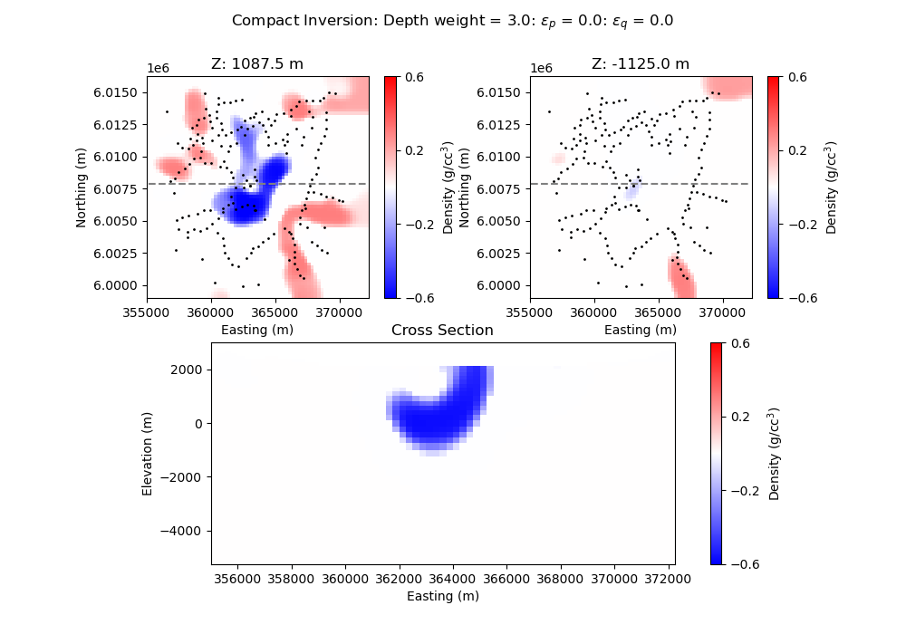 117 |
118 |
117 |
118 |  134 |
134 | 


