├── 01 - Data Preparation: Feature Engineering and AutoML.py
├── 02 - Data Exploration: Generated by AutoML.py
├── 03 - Best Trial Run: XGBoost training improvements.py
├── End-to-End ML Workshop DB SQL Dashboard.pdf
├── End-to-End ML Workshop.dbdash
└── README.md
/01 - Data Preparation: Feature Engineering and AutoML.py:
--------------------------------------------------------------------------------
1 | # Databricks notebook source
2 | # MAGIC %md
3 | # MAGIC ## End to End ML on Databricks
4 | # MAGIC
5 | # MAGIC  6 |
7 | # COMMAND ----------
8 |
9 | from pyspark.sql.functions import *
10 | from pyspark.sql.types import *
11 |
12 | import pyspark.pandas as pd
13 |
14 | # COMMAND ----------
15 |
16 | # MAGIC %md
17 | # MAGIC
18 | # MAGIC For this workshop we will use a publicly available adult dataset example found in `/databricks-datasets/`. We could also use Python or Spark to read data from databases or cloud storage.
19 |
20 | # COMMAND ----------
21 |
22 | # We can ls the directory and see what files we have available
23 | dbutils.fs.ls("/databricks-datasets/adult")
24 |
25 | # COMMAND ----------
26 |
27 | # MAGIC %md
28 | # MAGIC #### Path configs
29 |
30 | # COMMAND ----------
31 |
32 | # Set config for database name, file paths, and table names
33 | database_name = 'ml_income_workshop'
34 | user = dbutils.notebook.entry_point.getDbutils().notebook().getContext().tags().apply('user')
35 |
36 | # Paths for various Delta tables
37 | raw_tbl_path = '/home/{}/ml_income_workshop/raw/'.format(user)
38 | clean_tbl_path = '/home/{}/ml_income_workshop/clean/'.format(user)
39 | inference_tbl_path = '/home/{}/ml_income_workshop/inference/'.format(user)
40 |
41 | raw_tbl_name = 'raw_income'
42 | clean_tbl_name = 'clean_income'
43 | inference_tbl_name = 'inference_income'
44 |
45 | # Delete the old database and tables if needed
46 | spark.sql('DROP DATABASE IF EXISTS {} CASCADE'.format(database_name))
47 |
48 | # Create database to house tables
49 | spark.sql('CREATE DATABASE {}'.format(database_name))
50 | spark.sql('USE {}'.format(database_name))
51 |
52 | # Drop any old delta lake files if needed (e.g. re-running this notebook with the same path variables)
53 | dbutils.fs.rm(raw_tbl_path, recurse = True)
54 | dbutils.fs.rm(clean_tbl_path, recurse = True)
55 | dbutils.fs.rm(inference_tbl_path, recurse = True)
56 |
57 | # COMMAND ----------
58 |
59 | # MAGIC %md
60 | # MAGIC ### Exploratory Data Analysis
61 |
62 | # COMMAND ----------
63 |
64 | # MAGIC %md #### Reading in Data
65 |
66 | # COMMAND ----------
67 |
68 | # MAGIC %sh cat /dbfs/databricks-datasets/adult/README.md
69 |
70 | # COMMAND ----------
71 |
72 | census_income_path = "/databricks-datasets/adult/adult.data"
73 |
74 | # defining the schema for departure_delays
75 | census_income_schema = StructType([ \
76 | StructField("age", IntegerType(), True), \
77 | StructField("workclass", StringType(), True), \
78 | StructField("fnlwgt", DoubleType(), True), \
79 | StructField("education", StringType(), True), \
80 | StructField("education_num", DoubleType(), True), \
81 | StructField("marital_status", StringType(), True), \
82 | StructField("occupation", StringType(), True), \
83 | StructField("relationship", StringType(), True), \
84 | StructField("race", StringType(), True), \
85 | StructField("sex", StringType(), True), \
86 | StructField("capital_gain", DoubleType(), True), \
87 | StructField("capital_loss", DoubleType(), True), \
88 | StructField("hours_per_week", DoubleType(), True), \
89 | StructField("native_country", StringType(), True), \
90 | StructField("income", StringType(), True),
91 | ])
92 | raw_df = spark.read.schema(census_income_schema).options(header='false', delimiter=',').csv(census_income_path)
93 |
94 | display(raw_df)
95 |
96 | # COMMAND ----------
97 |
98 | raw_df.write.format('delta').mode('overwrite').save(raw_tbl_path)
99 |
100 | # COMMAND ----------
101 |
102 | display(raw_df)
103 |
104 | # COMMAND ----------
105 |
106 | # MAGIC %md By clicking on the `Data Profile` tab above we can easily generate descriptive statistics on our dataset. We can also call those results using `dbutils`
107 |
108 | # COMMAND ----------
109 |
110 | dbutils.data.summarize(raw_df)
111 |
112 | # COMMAND ----------
113 |
114 | # Create table to query with SQL
115 | spark.sql('''
116 | CREATE TABLE {0}
117 | USING DELTA
118 | LOCATION '{1}'
119 | '''.format(raw_tbl_name, raw_tbl_path)
120 | )
121 |
122 | # COMMAND ----------
123 |
124 | # MAGIC %md
125 | # MAGIC Now let's query our table with SQL!
126 |
127 | # COMMAND ----------
128 |
129 | # MAGIC %sql
130 | # MAGIC -- Occupations with the highest average age
131 | # MAGIC SELECT occupation, ROUND(AVG(age)) AS avg_age
132 | # MAGIC FROM raw_income
133 | # MAGIC GROUP BY occupation
134 | # MAGIC ORDER BY avg_age DESC
135 |
136 | # COMMAND ----------
137 |
138 | # MAGIC %md ### Data Visualization
139 |
140 | # COMMAND ----------
141 |
142 | # MAGIC %md We can also display the results as a table using the built-in visualizations
143 |
144 | # COMMAND ----------
145 |
146 | # MAGIC %sql
147 | # MAGIC -- Occupations with the highest average age
148 | # MAGIC SELECT occupation, ROUND(AVG(age)) AS avg_age
149 | # MAGIC FROM raw_income
150 | # MAGIC GROUP BY occupation
151 | # MAGIC ORDER BY avg_age DESC
152 |
153 | # COMMAND ----------
154 |
155 | # MAGIC %md
156 | # MAGIC You can also leverage [`Pandas on Spark`](https://spark.apache.org/docs/latest/api/python/user_guide/pandas_on_spark/index.html) to use your favorite pandas and matplotlib functions for data wrangling and visualization but with the scale and optimizations of Spark ([announcement blog](https://databricks.com/blog/2021/10/04/pandas-api-on-upcoming-apache-spark-3-2.html), [docs](https://spark.apache.org/docs/latest/api/python/user_guide/pandas_on_spark/index.html), [quickstart](https://spark.apache.org/docs/latest/api/python/getting_started/quickstart_ps.html))
157 | # MAGIC
158 | # MAGIC
6 |
7 | # COMMAND ----------
8 |
9 | from pyspark.sql.functions import *
10 | from pyspark.sql.types import *
11 |
12 | import pyspark.pandas as pd
13 |
14 | # COMMAND ----------
15 |
16 | # MAGIC %md
17 | # MAGIC
18 | # MAGIC For this workshop we will use a publicly available adult dataset example found in `/databricks-datasets/`. We could also use Python or Spark to read data from databases or cloud storage.
19 |
20 | # COMMAND ----------
21 |
22 | # We can ls the directory and see what files we have available
23 | dbutils.fs.ls("/databricks-datasets/adult")
24 |
25 | # COMMAND ----------
26 |
27 | # MAGIC %md
28 | # MAGIC #### Path configs
29 |
30 | # COMMAND ----------
31 |
32 | # Set config for database name, file paths, and table names
33 | database_name = 'ml_income_workshop'
34 | user = dbutils.notebook.entry_point.getDbutils().notebook().getContext().tags().apply('user')
35 |
36 | # Paths for various Delta tables
37 | raw_tbl_path = '/home/{}/ml_income_workshop/raw/'.format(user)
38 | clean_tbl_path = '/home/{}/ml_income_workshop/clean/'.format(user)
39 | inference_tbl_path = '/home/{}/ml_income_workshop/inference/'.format(user)
40 |
41 | raw_tbl_name = 'raw_income'
42 | clean_tbl_name = 'clean_income'
43 | inference_tbl_name = 'inference_income'
44 |
45 | # Delete the old database and tables if needed
46 | spark.sql('DROP DATABASE IF EXISTS {} CASCADE'.format(database_name))
47 |
48 | # Create database to house tables
49 | spark.sql('CREATE DATABASE {}'.format(database_name))
50 | spark.sql('USE {}'.format(database_name))
51 |
52 | # Drop any old delta lake files if needed (e.g. re-running this notebook with the same path variables)
53 | dbutils.fs.rm(raw_tbl_path, recurse = True)
54 | dbutils.fs.rm(clean_tbl_path, recurse = True)
55 | dbutils.fs.rm(inference_tbl_path, recurse = True)
56 |
57 | # COMMAND ----------
58 |
59 | # MAGIC %md
60 | # MAGIC ### Exploratory Data Analysis
61 |
62 | # COMMAND ----------
63 |
64 | # MAGIC %md #### Reading in Data
65 |
66 | # COMMAND ----------
67 |
68 | # MAGIC %sh cat /dbfs/databricks-datasets/adult/README.md
69 |
70 | # COMMAND ----------
71 |
72 | census_income_path = "/databricks-datasets/adult/adult.data"
73 |
74 | # defining the schema for departure_delays
75 | census_income_schema = StructType([ \
76 | StructField("age", IntegerType(), True), \
77 | StructField("workclass", StringType(), True), \
78 | StructField("fnlwgt", DoubleType(), True), \
79 | StructField("education", StringType(), True), \
80 | StructField("education_num", DoubleType(), True), \
81 | StructField("marital_status", StringType(), True), \
82 | StructField("occupation", StringType(), True), \
83 | StructField("relationship", StringType(), True), \
84 | StructField("race", StringType(), True), \
85 | StructField("sex", StringType(), True), \
86 | StructField("capital_gain", DoubleType(), True), \
87 | StructField("capital_loss", DoubleType(), True), \
88 | StructField("hours_per_week", DoubleType(), True), \
89 | StructField("native_country", StringType(), True), \
90 | StructField("income", StringType(), True),
91 | ])
92 | raw_df = spark.read.schema(census_income_schema).options(header='false', delimiter=',').csv(census_income_path)
93 |
94 | display(raw_df)
95 |
96 | # COMMAND ----------
97 |
98 | raw_df.write.format('delta').mode('overwrite').save(raw_tbl_path)
99 |
100 | # COMMAND ----------
101 |
102 | display(raw_df)
103 |
104 | # COMMAND ----------
105 |
106 | # MAGIC %md By clicking on the `Data Profile` tab above we can easily generate descriptive statistics on our dataset. We can also call those results using `dbutils`
107 |
108 | # COMMAND ----------
109 |
110 | dbutils.data.summarize(raw_df)
111 |
112 | # COMMAND ----------
113 |
114 | # Create table to query with SQL
115 | spark.sql('''
116 | CREATE TABLE {0}
117 | USING DELTA
118 | LOCATION '{1}'
119 | '''.format(raw_tbl_name, raw_tbl_path)
120 | )
121 |
122 | # COMMAND ----------
123 |
124 | # MAGIC %md
125 | # MAGIC Now let's query our table with SQL!
126 |
127 | # COMMAND ----------
128 |
129 | # MAGIC %sql
130 | # MAGIC -- Occupations with the highest average age
131 | # MAGIC SELECT occupation, ROUND(AVG(age)) AS avg_age
132 | # MAGIC FROM raw_income
133 | # MAGIC GROUP BY occupation
134 | # MAGIC ORDER BY avg_age DESC
135 |
136 | # COMMAND ----------
137 |
138 | # MAGIC %md ### Data Visualization
139 |
140 | # COMMAND ----------
141 |
142 | # MAGIC %md We can also display the results as a table using the built-in visualizations
143 |
144 | # COMMAND ----------
145 |
146 | # MAGIC %sql
147 | # MAGIC -- Occupations with the highest average age
148 | # MAGIC SELECT occupation, ROUND(AVG(age)) AS avg_age
149 | # MAGIC FROM raw_income
150 | # MAGIC GROUP BY occupation
151 | # MAGIC ORDER BY avg_age DESC
152 |
153 | # COMMAND ----------
154 |
155 | # MAGIC %md
156 | # MAGIC You can also leverage [`Pandas on Spark`](https://spark.apache.org/docs/latest/api/python/user_guide/pandas_on_spark/index.html) to use your favorite pandas and matplotlib functions for data wrangling and visualization but with the scale and optimizations of Spark ([announcement blog](https://databricks.com/blog/2021/10/04/pandas-api-on-upcoming-apache-spark-3-2.html), [docs](https://spark.apache.org/docs/latest/api/python/user_guide/pandas_on_spark/index.html), [quickstart](https://spark.apache.org/docs/latest/api/python/getting_started/quickstart_ps.html))
157 | # MAGIC
158 | # MAGIC  159 |
160 | # COMMAND ----------
161 |
162 | # convert our raw spark distributed dataframe into a distributed pandas dataframe
163 | raw_df_pdf = raw_df.to_pandas_on_spark()
164 |
165 | # perform the same aggregation we did in SQL using familiar Pandas syntax
166 | avg_age_by_occupation = raw_df_pdf.groupby("occupation").mean().round().reset_index()[["occupation", "age"]].sort_values("age", ascending = False)
167 |
168 | # re-create the same plot using familiar pandas and matplotlib syntax distributed with Spark
169 | avg_age_by_occupation.plot(kind = "bar", x = "occupation", y = "age")
170 |
171 | # COMMAND ----------
172 |
173 | # MAGIC %md
174 | # MAGIC #### Data Wrangling
175 | # MAGIC We can leverage [`Pandas on Spark`](https://spark.apache.org/docs/latest/api/python/user_guide/pandas_on_spark/index.html) to clean and wrangle our data at scale. We are going to drop missing values and clean up category values.
176 |
177 | # COMMAND ----------
178 |
179 | # Drop missing values
180 | clean_pdf = raw_df_pdf.dropna(axis = 0, how = 'any')
181 |
182 | def category_cleaner(value):
183 | return value.strip().lower().replace('.', '').replace(',', '').replace(' ', '-')
184 |
185 | categorical_cols = ['workclass', 'education', 'marital_status', 'occupation', 'relationship', 'race', 'sex', 'native_country', 'income']
186 |
187 | for column in categorical_cols:
188 | clean_pdf[column] = clean_pdf[column].apply(lambda value: category_cleaner(value))
189 |
190 | # COMMAND ----------
191 |
192 | # MAGIC %md
193 | # MAGIC #### Feature Engineering
194 | # MAGIC
195 | # MAGIC * Bin the age into decades (min age 17 to max age 90)
196 | # MAGIC * take the log of features with skewed distributions (capital_gain, capital_loss)
197 |
198 | # COMMAND ----------
199 |
200 | import numpy as np
201 |
202 | # bin age into decades
203 | def bin_age(value):
204 | if value <= 19:
205 | return "teens"
206 | elif value in range(20,30):
207 | return "20s"
208 | elif value in range(30,40):
209 | return "30s"
210 | elif value in range(40,50):
211 | return "40s"
212 | elif value in range(50,60):
213 | return "50s"
214 | elif value in range(60,100):
215 | return "60+"
216 | else:
217 | return "other"
218 |
219 | clean_pdf['age_by_decade'] = clean_pdf['age'].apply(bin_age)
220 |
221 | # Take the log of features with skewed distributions
222 | def log_transform(value):
223 | return float(np.log(value + 1)) # for 0 values
224 |
225 | clean_pdf['log_capital_gain'] = clean_pdf['capital_gain'].apply(log_transform)
226 | clean_pdf['log_capital_loss'] = clean_pdf['capital_loss'].apply(log_transform)
227 |
228 | # Drop columns
229 | clean_pdf = clean_pdf.drop(['age', 'capital_gain', 'capital_loss'], axis = 1)
230 |
231 | display(clean_pdf.head(3))
232 |
233 | # COMMAND ----------
234 |
235 | # we are now going to save this cleaned table as a delta file in our cloud storage and create a metadata table on top of it
236 | clean_pdf.to_delta(clean_tbl_path)
237 |
238 | spark.sql('''
239 | CREATE TABLE {0}
240 | USING DELTA
241 | LOCATION '{1}'
242 | '''.format(clean_tbl_name, clean_tbl_path)
243 | )
244 |
245 | # COMMAND ----------
246 |
247 | # MAGIC %sql
248 | # MAGIC SELECT *
249 | # MAGIC FROM clean_income
250 | # MAGIC LIMIT 3
251 |
252 | # COMMAND ----------
253 |
254 | # MAGIC %md
255 | # MAGIC Let's package the all the data processing into a function for later use
256 |
257 | # COMMAND ----------
258 |
259 | def process_census_data(dataframe):
260 | """
261 | Function to wrap specific processing for census data tables
262 | Input and output is a pyspark.pandas dataframe
263 | """
264 | categorical_cols = ['workclass', 'education', 'marital_status',
265 | 'occupation', 'relationship', 'race', 'sex',
266 | 'native_country', 'income']
267 |
268 | # categorical column cleansing
269 | for column in categorical_cols:
270 | dataframe[column] = dataframe[column].apply(lambda value: category_cleaner(value))
271 |
272 | # bin age
273 | dataframe['age_by_decade'] = dataframe['age'].apply(bin_age)
274 |
275 | # log transform
276 | dataframe['log_capital_gain'] = dataframe['capital_gain'].apply(log_transform)
277 | dataframe['log_capital_loss'] = dataframe['capital_loss'].apply(log_transform)
278 |
279 | # Drop columns
280 | dataframe = dataframe.drop(['age', 'capital_gain', 'capital_loss'], axis = 1)
281 |
282 | return dataframe
283 |
284 | # COMMAND ----------
285 |
286 | # MAGIC %md
287 | # MAGIC Last but not least, let's create the same transformations to our inference dataset for testing later
288 |
289 | # COMMAND ----------
290 |
291 | census_income_test_path = "/databricks-datasets/adult/adult.test"
292 |
293 | inference_pdf = (spark.read.schema(census_income_schema)
294 | .options(header='false', delimiter=',')
295 | .csv(census_income_test_path)
296 | .to_pandas_on_spark()
297 | )
298 |
299 | inference_pdf = process_census_data(inference_pdf)
300 | inference_pdf.to_delta(inference_tbl_path)
301 |
302 | spark.sql('''
303 | CREATE TABLE {0}
304 | USING DELTA
305 | LOCATION '{1}'
306 | '''.format(inference_tbl_name, inference_tbl_path)
307 | )
308 |
309 | # COMMAND ----------
310 |
311 | # MAGIC %md
312 | # MAGIC Great! Our dataset is ready for us to use with AutoML to train a benchmark model.
313 |
314 | # COMMAND ----------
315 |
316 | # MAGIC %md
317 | # MAGIC ### AutoML
318 | # MAGIC
319 | # MAGIC
159 |
160 | # COMMAND ----------
161 |
162 | # convert our raw spark distributed dataframe into a distributed pandas dataframe
163 | raw_df_pdf = raw_df.to_pandas_on_spark()
164 |
165 | # perform the same aggregation we did in SQL using familiar Pandas syntax
166 | avg_age_by_occupation = raw_df_pdf.groupby("occupation").mean().round().reset_index()[["occupation", "age"]].sort_values("age", ascending = False)
167 |
168 | # re-create the same plot using familiar pandas and matplotlib syntax distributed with Spark
169 | avg_age_by_occupation.plot(kind = "bar", x = "occupation", y = "age")
170 |
171 | # COMMAND ----------
172 |
173 | # MAGIC %md
174 | # MAGIC #### Data Wrangling
175 | # MAGIC We can leverage [`Pandas on Spark`](https://spark.apache.org/docs/latest/api/python/user_guide/pandas_on_spark/index.html) to clean and wrangle our data at scale. We are going to drop missing values and clean up category values.
176 |
177 | # COMMAND ----------
178 |
179 | # Drop missing values
180 | clean_pdf = raw_df_pdf.dropna(axis = 0, how = 'any')
181 |
182 | def category_cleaner(value):
183 | return value.strip().lower().replace('.', '').replace(',', '').replace(' ', '-')
184 |
185 | categorical_cols = ['workclass', 'education', 'marital_status', 'occupation', 'relationship', 'race', 'sex', 'native_country', 'income']
186 |
187 | for column in categorical_cols:
188 | clean_pdf[column] = clean_pdf[column].apply(lambda value: category_cleaner(value))
189 |
190 | # COMMAND ----------
191 |
192 | # MAGIC %md
193 | # MAGIC #### Feature Engineering
194 | # MAGIC
195 | # MAGIC * Bin the age into decades (min age 17 to max age 90)
196 | # MAGIC * take the log of features with skewed distributions (capital_gain, capital_loss)
197 |
198 | # COMMAND ----------
199 |
200 | import numpy as np
201 |
202 | # bin age into decades
203 | def bin_age(value):
204 | if value <= 19:
205 | return "teens"
206 | elif value in range(20,30):
207 | return "20s"
208 | elif value in range(30,40):
209 | return "30s"
210 | elif value in range(40,50):
211 | return "40s"
212 | elif value in range(50,60):
213 | return "50s"
214 | elif value in range(60,100):
215 | return "60+"
216 | else:
217 | return "other"
218 |
219 | clean_pdf['age_by_decade'] = clean_pdf['age'].apply(bin_age)
220 |
221 | # Take the log of features with skewed distributions
222 | def log_transform(value):
223 | return float(np.log(value + 1)) # for 0 values
224 |
225 | clean_pdf['log_capital_gain'] = clean_pdf['capital_gain'].apply(log_transform)
226 | clean_pdf['log_capital_loss'] = clean_pdf['capital_loss'].apply(log_transform)
227 |
228 | # Drop columns
229 | clean_pdf = clean_pdf.drop(['age', 'capital_gain', 'capital_loss'], axis = 1)
230 |
231 | display(clean_pdf.head(3))
232 |
233 | # COMMAND ----------
234 |
235 | # we are now going to save this cleaned table as a delta file in our cloud storage and create a metadata table on top of it
236 | clean_pdf.to_delta(clean_tbl_path)
237 |
238 | spark.sql('''
239 | CREATE TABLE {0}
240 | USING DELTA
241 | LOCATION '{1}'
242 | '''.format(clean_tbl_name, clean_tbl_path)
243 | )
244 |
245 | # COMMAND ----------
246 |
247 | # MAGIC %sql
248 | # MAGIC SELECT *
249 | # MAGIC FROM clean_income
250 | # MAGIC LIMIT 3
251 |
252 | # COMMAND ----------
253 |
254 | # MAGIC %md
255 | # MAGIC Let's package the all the data processing into a function for later use
256 |
257 | # COMMAND ----------
258 |
259 | def process_census_data(dataframe):
260 | """
261 | Function to wrap specific processing for census data tables
262 | Input and output is a pyspark.pandas dataframe
263 | """
264 | categorical_cols = ['workclass', 'education', 'marital_status',
265 | 'occupation', 'relationship', 'race', 'sex',
266 | 'native_country', 'income']
267 |
268 | # categorical column cleansing
269 | for column in categorical_cols:
270 | dataframe[column] = dataframe[column].apply(lambda value: category_cleaner(value))
271 |
272 | # bin age
273 | dataframe['age_by_decade'] = dataframe['age'].apply(bin_age)
274 |
275 | # log transform
276 | dataframe['log_capital_gain'] = dataframe['capital_gain'].apply(log_transform)
277 | dataframe['log_capital_loss'] = dataframe['capital_loss'].apply(log_transform)
278 |
279 | # Drop columns
280 | dataframe = dataframe.drop(['age', 'capital_gain', 'capital_loss'], axis = 1)
281 |
282 | return dataframe
283 |
284 | # COMMAND ----------
285 |
286 | # MAGIC %md
287 | # MAGIC Last but not least, let's create the same transformations to our inference dataset for testing later
288 |
289 | # COMMAND ----------
290 |
291 | census_income_test_path = "/databricks-datasets/adult/adult.test"
292 |
293 | inference_pdf = (spark.read.schema(census_income_schema)
294 | .options(header='false', delimiter=',')
295 | .csv(census_income_test_path)
296 | .to_pandas_on_spark()
297 | )
298 |
299 | inference_pdf = process_census_data(inference_pdf)
300 | inference_pdf.to_delta(inference_tbl_path)
301 |
302 | spark.sql('''
303 | CREATE TABLE {0}
304 | USING DELTA
305 | LOCATION '{1}'
306 | '''.format(inference_tbl_name, inference_tbl_path)
307 | )
308 |
309 | # COMMAND ----------
310 |
311 | # MAGIC %md
312 | # MAGIC Great! Our dataset is ready for us to use with AutoML to train a benchmark model.
313 |
314 | # COMMAND ----------
315 |
316 | # MAGIC %md
317 | # MAGIC ### AutoML
318 | # MAGIC
319 | # MAGIC 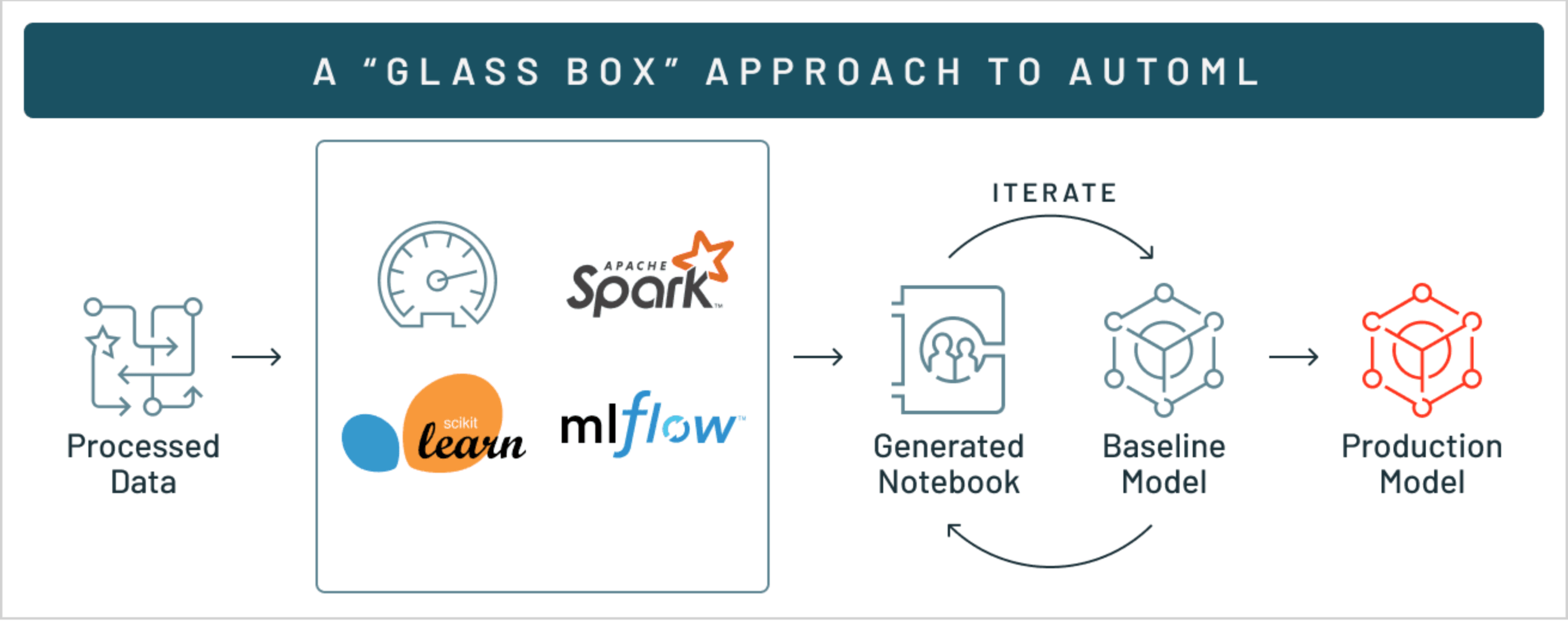 320 |
321 | # COMMAND ----------
322 |
323 | # MAGIC %md
324 | # MAGIC Now let's create a glassbox AutoML model to help us automatically test different models and parameters and reduce time manually testing and tweaking ML models. We can run AutoML via the `databricks.automl` library or via the UI by creating a new [mlflow automl experiment](#mlflow/experiments).
325 | # MAGIC
326 | # MAGIC Here, we'll run AutoML in the next cell.
327 |
328 | # COMMAND ----------
329 |
330 | import databricks.automl
331 |
332 | summary = databricks.automl.classify(clean_pdf, target_col='income', primary_metric="f1", data_dir='dbfs:/automl/ml_income_workshop', timeout_minutes=5)
333 |
334 | # COMMAND ----------
335 |
336 | # MAGIC %md
337 | # MAGIC Check out the screenshots below that walk through this process via the UI.
338 | # MAGIC
339 | # MAGIC
320 |
321 | # COMMAND ----------
322 |
323 | # MAGIC %md
324 | # MAGIC Now let's create a glassbox AutoML model to help us automatically test different models and parameters and reduce time manually testing and tweaking ML models. We can run AutoML via the `databricks.automl` library or via the UI by creating a new [mlflow automl experiment](#mlflow/experiments).
325 | # MAGIC
326 | # MAGIC Here, we'll run AutoML in the next cell.
327 |
328 | # COMMAND ----------
329 |
330 | import databricks.automl
331 |
332 | summary = databricks.automl.classify(clean_pdf, target_col='income', primary_metric="f1", data_dir='dbfs:/automl/ml_income_workshop', timeout_minutes=5)
333 |
334 | # COMMAND ----------
335 |
336 | # MAGIC %md
337 | # MAGIC Check out the screenshots below that walk through this process via the UI.
338 | # MAGIC
339 | # MAGIC 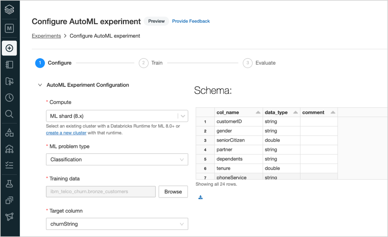
 340 |
--------------------------------------------------------------------------------
/02 - Data Exploration: Generated by AutoML.py:
--------------------------------------------------------------------------------
1 | # Databricks notebook source
2 | # MAGIC %md
3 | # MAGIC # Data Exploration
4 | # MAGIC This notebook performs exploratory data analysis on the dataset.
5 | # MAGIC To expand on the analysis, attach this notebook to the **ml-workshop-2.0** cluster,
6 | # MAGIC edit [the options of pandas-profiling](https://pandas-profiling.github.io/pandas-profiling/docs/master/rtd/pages/advanced_usage.html), and rerun it.
7 | # MAGIC - Explore completed trials in the [MLflow experiment](#mlflow/experiments/2984496825650690/s?orderByKey=metrics.%60val_f1_score%60&orderByAsc=false)
8 | # MAGIC - Navigate to the parent notebook [here](#notebook/2984496825649216) (If you launched the AutoML experiment using the Experiments UI, this link isn't very useful.)
9 | # MAGIC
10 | # MAGIC Runtime Version: _10.2.x-cpu-ml-scala2.12_
11 |
12 | # COMMAND ----------
13 |
14 | # Load the data into a pandas DataFrame
15 | import pandas as pd
16 | import databricks.automl_runtime
17 |
18 | df = pd.read_parquet("file:///dbfs/automl/ml_income_workshop/22-02-18-07:07/62666dbf")
19 |
20 | target_col = "income"
21 |
22 | # COMMAND ----------
23 |
24 | # MAGIC %md
25 | # MAGIC ## Profiling Results
26 |
27 | # COMMAND ----------
28 |
29 | from pandas_profiling import ProfileReport
30 | df_profile = ProfileReport(df, title="Profiling Report", progress_bar=False, infer_dtypes=False)
31 | profile_html = df_profile.to_html()
32 |
33 | displayHTML(profile_html)
34 |
--------------------------------------------------------------------------------
/03 - Best Trial Run: XGBoost training improvements.py:
--------------------------------------------------------------------------------
1 | # Databricks notebook source
2 | # MAGIC %md
3 | # MAGIC # XGBoost training
4 | # MAGIC This is an auto-generated notebook. To reproduce these results, attach this notebook to the **ml-workshop-2.0** cluster and rerun it.
5 | # MAGIC - Compare trials in the [MLflow experiment](#mlflow/experiments/4212189882465177/s?orderByKey=metrics.%60val_f1_score%60&orderByAsc=false)
6 | # MAGIC - Navigate to the parent notebook [here](#notebook/4212189882465089) (If you launched the AutoML experiment using the Experiments UI, this link isn't very useful.)
7 | # MAGIC - Clone this notebook into your project folder by selecting **File > Clone** in the notebook toolbar.
8 | # MAGIC
9 | # MAGIC Runtime Version: _10.2.x-cpu-ml-scala2.12_
10 |
11 | # COMMAND ----------
12 |
13 | # MAGIC %md
14 | # MAGIC **Be sure to update the mlflow experiment path appropriately!**
15 |
16 | # COMMAND ----------
17 |
18 | import mlflow
19 | import databricks.automl_runtime
20 |
21 | from pyspark.sql.functions import *
22 |
23 | # Use MLflow to track experiments
24 | mlflow.set_experiment("/Shared/ML-Workshop-2.0/End-to-End-ML/ml-workshop-income-classifier")
25 |
26 | target_col = "income"
27 | database_name = 'ml_income_workshop'
28 | user = dbutils.notebook.entry_point.getDbutils().notebook().getContext().tags().apply('user')
29 |
30 |
31 | # COMMAND ----------
32 |
33 | # MAGIC %md
34 | # MAGIC ## Load Data
35 |
36 | # COMMAND ----------
37 |
38 | # Load input data into a pandas DataFrame.
39 | import pandas as pd
40 | df_loaded = spark.table("ml_income_workshop.clean_income").toPandas()
41 |
42 | ## Data to be Scored
43 | inference_data = spark.read.table('ml_income_workshop.inference_income').toPandas()
44 |
45 | # Preview data
46 | df_loaded.head(5)
47 |
48 | # COMMAND ----------
49 |
50 | # MAGIC %md
51 | # MAGIC ### Select supported columns
52 | # MAGIC Select only the columns that are supported. This allows us to train a model that can predict on a dataset that has extra columns that are not used in training.
53 | # MAGIC `[]` are dropped in the pipelines. See the Alerts tab of the AutoML Experiment page for details on why these columns are dropped.
54 |
55 | # COMMAND ----------
56 |
57 | from databricks.automl_runtime.sklearn.column_selector import ColumnSelector
58 | supported_cols = ["age_by_decade", "fnlwgt", "education", "occupation", "hours_per_week", "relationship", "workclass", "log_capital_gain", "log_capital_loss", "native_country"]
59 | col_selector = ColumnSelector(supported_cols)
60 |
61 | # COMMAND ----------
62 |
63 | # MAGIC %md
64 | # MAGIC ## Preprocessors
65 |
66 | # COMMAND ----------
67 |
68 | transformers = []
69 |
70 | # COMMAND ----------
71 |
72 | # MAGIC %md
73 | # MAGIC ### Incorporating insights from Data Exploration Notebook
74 | # MAGIC
75 | # MAGIC According to the data exploration notebook, we have a few features with high correlation. We can try dropping some of these features to reduce redundant information. We'll also drop features with little correlation to the income column.
76 | # MAGIC
77 | # MAGIC In this case, we'll drop the `workclass`, `sex`, `race`, `education_num`, and `marital_status` columns
78 |
79 | # COMMAND ----------
80 |
81 | df_loaded.drop(["workclass", "sex", "race", "education_num", "marital_status"], axis=1)
82 |
83 | # COMMAND ----------
84 |
85 | # MAGIC %md
86 | # MAGIC ### Numerical columns
87 | # MAGIC
88 | # MAGIC Missing values for numerical columns are imputed with mean for consistency
89 |
90 | # COMMAND ----------
91 |
92 | from sklearn.impute import SimpleImputer
93 | from sklearn.pipeline import Pipeline
94 | from sklearn.preprocessing import FunctionTransformer
95 |
96 | numerical_pipeline = Pipeline(steps=[
97 | ("converter", FunctionTransformer(lambda df: df.apply(pd.to_numeric, errors="coerce"))),
98 | ("imputer", SimpleImputer(strategy="mean"))
99 | ])
100 |
101 | transformers.append(("numerical", numerical_pipeline, ["fnlwgt", "hours_per_week", "log_capital_gain", "log_capital_loss"]))
102 |
103 | # COMMAND ----------
104 |
105 | # MAGIC %md
106 | # MAGIC ### Categorical columns
107 |
108 | # COMMAND ----------
109 |
110 | # MAGIC %md
111 | # MAGIC #### Low-cardinality categoricals
112 | # MAGIC Convert each low-cardinality categorical column into multiple binary columns through one-hot encoding.
113 | # MAGIC For each input categorical column (string or numeric), the number of output columns is equal to the number of unique values in the input column.
114 |
115 | # COMMAND ----------
116 |
117 | from sklearn.pipeline import Pipeline
118 | from sklearn.preprocessing import OneHotEncoder
119 |
120 | one_hot_encoder = OneHotEncoder(handle_unknown="ignore")
121 |
122 | transformers.append(("onehot", one_hot_encoder, ["age_by_decade", "education", "occupation", "relationship", "workclass", "native_country"]))
123 |
124 | # COMMAND ----------
125 |
126 | from sklearn.compose import ColumnTransformer
127 |
128 | preprocessor = ColumnTransformer(transformers, remainder="passthrough", sparse_threshold=0)
129 |
130 | # COMMAND ----------
131 |
132 | # MAGIC %md
133 | # MAGIC ### Feature standardization
134 | # MAGIC Scale all feature columns to be centered around zero with unit variance.
135 |
136 | # COMMAND ----------
137 |
138 | from sklearn.preprocessing import StandardScaler
139 |
140 | standardizer = StandardScaler()
141 |
142 | # COMMAND ----------
143 |
144 | # MAGIC %md
145 | # MAGIC ## Train - Validation - Split
146 | # MAGIC Split the input data into 2 sets:
147 | # MAGIC - Train (80% of the dataset used to train the model)
148 | # MAGIC - Validation (20% of the dataset used to tune the hyperparameters of the model)
149 |
150 | # COMMAND ----------
151 |
152 | from sklearn.model_selection import train_test_split
153 |
154 | split_X = df_loaded.drop([target_col], axis=1)
155 | split_y = df_loaded[target_col]
156 |
157 | # Split out train data
158 | X_train, X_val, y_train, y_val = train_test_split(split_X, split_y, train_size=0.8, random_state=149849802, stratify=split_y)
159 |
160 |
161 | # COMMAND ----------
162 |
163 | X_test = inference_data.drop([target_col], axis=1)
164 | y_test = inference_data[target_col]
165 |
166 | # COMMAND ----------
167 |
168 | # MAGIC %md
169 | # MAGIC ## Train classification model
170 | # MAGIC - Log relevant metrics to MLflow to track runs
171 | # MAGIC - All the runs are logged under [this MLflow experiment](#mlflow/experiments/4212189882465177/s?orderByKey=metrics.%60val_f1_score%60&orderByAsc=false)
172 | # MAGIC - Change the model parameters and re-run the training cell to log a different trial to the MLflow experiment
173 | # MAGIC - To view the full list of tunable hyperparameters, check the output of the cell below
174 |
175 | # COMMAND ----------
176 |
177 | from xgboost import XGBClassifier
178 |
179 | help(XGBClassifier)
180 |
181 | # COMMAND ----------
182 |
183 | # MAGIC %md
184 | # MAGIC ### Incorporating insights from Data Exploration: Downsampling
185 |
186 | # COMMAND ----------
187 |
188 | # RandomUnderSampler for class imbalance (decrease <=50K label count)
189 | from imblearn.under_sampling import RandomUnderSampler
190 |
191 | # From our data exploration notebook, class ratio looks like 75/25 (<=50k/>=50k)
192 | undersampler = RandomUnderSampler(random_state=42)
193 |
194 | # COMMAND ----------
195 |
196 | import mlflow
197 | import sklearn
198 | from sklearn import set_config
199 | from imblearn.pipeline import make_pipeline
200 |
201 | set_config(display="diagram")
202 |
203 | xgbc_classifier = XGBClassifier(
204 | colsample_bytree=0.5562503325532802,
205 | learning_rate=0.26571572922086373,
206 | max_depth=5,
207 | min_child_weight=5,
208 | n_estimators=30,
209 | n_jobs=100,
210 | subsample=0.6859242756647854,
211 | verbosity=0,
212 | random_state=149849802,
213 | )
214 |
215 | model = make_pipeline(col_selector, preprocessor, standardizer, undersampler, xgbc_classifier)
216 |
217 | model
218 |
219 | # COMMAND ----------
220 |
221 | # Enable automatic logging of input samples, metrics, parameters, and models
222 | mlflow.sklearn.autolog(log_input_examples=True, silent=True)
223 |
224 | with mlflow.start_run(run_name="xgboost") as mlflow_run:
225 | model.fit(X_train, y_train)
226 |
227 | # Training metrics are logged by MLflow autologging
228 | # Log metrics for the validation set
229 | xgbc_val_metrics = mlflow.sklearn.eval_and_log_metrics(model, X_val, y_val, prefix="val_")
230 |
231 | # Log metrics for the test set
232 | xgbc_test_metrics = mlflow.sklearn.eval_and_log_metrics(model, X_test, y_test, prefix="test_")
233 |
234 | # Display the logged metrics
235 | xgbc_val_metrics = {k.replace("val_", ""): v for k, v in xgbc_val_metrics.items()}
236 | xgbc_test_metrics = {k.replace("test_", ""): v for k, v in xgbc_test_metrics.items()}
237 |
238 | metrics_pdf = pd.DataFrame([xgbc_val_metrics, xgbc_test_metrics], index=["validation", "test"])
239 | metrics_pdf["dataset"] = ["ml_income_workshop.clean_income", "ml_income_workshop.inference_income"]
240 | metrics_df = spark.createDataFrame(metrics_pdf)
241 | display(metrics_df)
242 |
243 | # COMMAND ----------
244 |
245 | # Save metrics to a delta table
246 | metrics_df.write.mode("overwrite").saveAsTable(f"{database_name}.metric_data_bronze")
247 |
248 | # COMMAND ----------
249 |
250 | # Patch requisite packages to the model environment YAML for model serving
251 | import os
252 | import shutil
253 | import uuid
254 | import yaml
255 |
256 | None
257 |
258 | import xgboost
259 | from mlflow.tracking import MlflowClient
260 |
261 | xgbc_temp_dir = os.path.join(os.environ["SPARK_LOCAL_DIRS"], str(uuid.uuid4())[:8])
262 | os.makedirs(xgbc_temp_dir)
263 | xgbc_client = MlflowClient()
264 | xgbc_model_env_path = xgbc_client.download_artifacts(mlflow_run.info.run_id, "model/conda.yaml", xgbc_temp_dir)
265 | xgbc_model_env_str = open(xgbc_model_env_path)
266 | xgbc_parsed_model_env_str = yaml.load(xgbc_model_env_str, Loader=yaml.FullLoader)
267 |
268 | xgbc_parsed_model_env_str["dependencies"][-1]["pip"].append(f"xgboost=={xgboost.__version__}")
269 |
270 | with open(xgbc_model_env_path, "w") as f:
271 | f.write(yaml.dump(xgbc_parsed_model_env_str))
272 | xgbc_client.log_artifact(run_id=mlflow_run.info.run_id, local_path=xgbc_model_env_path, artifact_path="model")
273 | shutil.rmtree(xgbc_temp_dir)
274 |
275 | # COMMAND ----------
276 |
277 | # MAGIC %md
278 | # MAGIC ## Feature importance
279 | # MAGIC
280 | # MAGIC SHAP is a game-theoretic approach to explain machine learning models, providing a summary plot
281 | # MAGIC of the relationship between features and model output. Features are ranked in descending order of
282 | # MAGIC importance, and impact/color describe the correlation between the feature and the target variable.
283 | # MAGIC - Generating SHAP feature importance is a very memory intensive operation, so to ensure that AutoML can run trials without
284 | # MAGIC running out of memory, we disable SHAP by default.
340 |
--------------------------------------------------------------------------------
/02 - Data Exploration: Generated by AutoML.py:
--------------------------------------------------------------------------------
1 | # Databricks notebook source
2 | # MAGIC %md
3 | # MAGIC # Data Exploration
4 | # MAGIC This notebook performs exploratory data analysis on the dataset.
5 | # MAGIC To expand on the analysis, attach this notebook to the **ml-workshop-2.0** cluster,
6 | # MAGIC edit [the options of pandas-profiling](https://pandas-profiling.github.io/pandas-profiling/docs/master/rtd/pages/advanced_usage.html), and rerun it.
7 | # MAGIC - Explore completed trials in the [MLflow experiment](#mlflow/experiments/2984496825650690/s?orderByKey=metrics.%60val_f1_score%60&orderByAsc=false)
8 | # MAGIC - Navigate to the parent notebook [here](#notebook/2984496825649216) (If you launched the AutoML experiment using the Experiments UI, this link isn't very useful.)
9 | # MAGIC
10 | # MAGIC Runtime Version: _10.2.x-cpu-ml-scala2.12_
11 |
12 | # COMMAND ----------
13 |
14 | # Load the data into a pandas DataFrame
15 | import pandas as pd
16 | import databricks.automl_runtime
17 |
18 | df = pd.read_parquet("file:///dbfs/automl/ml_income_workshop/22-02-18-07:07/62666dbf")
19 |
20 | target_col = "income"
21 |
22 | # COMMAND ----------
23 |
24 | # MAGIC %md
25 | # MAGIC ## Profiling Results
26 |
27 | # COMMAND ----------
28 |
29 | from pandas_profiling import ProfileReport
30 | df_profile = ProfileReport(df, title="Profiling Report", progress_bar=False, infer_dtypes=False)
31 | profile_html = df_profile.to_html()
32 |
33 | displayHTML(profile_html)
34 |
--------------------------------------------------------------------------------
/03 - Best Trial Run: XGBoost training improvements.py:
--------------------------------------------------------------------------------
1 | # Databricks notebook source
2 | # MAGIC %md
3 | # MAGIC # XGBoost training
4 | # MAGIC This is an auto-generated notebook. To reproduce these results, attach this notebook to the **ml-workshop-2.0** cluster and rerun it.
5 | # MAGIC - Compare trials in the [MLflow experiment](#mlflow/experiments/4212189882465177/s?orderByKey=metrics.%60val_f1_score%60&orderByAsc=false)
6 | # MAGIC - Navigate to the parent notebook [here](#notebook/4212189882465089) (If you launched the AutoML experiment using the Experiments UI, this link isn't very useful.)
7 | # MAGIC - Clone this notebook into your project folder by selecting **File > Clone** in the notebook toolbar.
8 | # MAGIC
9 | # MAGIC Runtime Version: _10.2.x-cpu-ml-scala2.12_
10 |
11 | # COMMAND ----------
12 |
13 | # MAGIC %md
14 | # MAGIC **Be sure to update the mlflow experiment path appropriately!**
15 |
16 | # COMMAND ----------
17 |
18 | import mlflow
19 | import databricks.automl_runtime
20 |
21 | from pyspark.sql.functions import *
22 |
23 | # Use MLflow to track experiments
24 | mlflow.set_experiment("/Shared/ML-Workshop-2.0/End-to-End-ML/ml-workshop-income-classifier")
25 |
26 | target_col = "income"
27 | database_name = 'ml_income_workshop'
28 | user = dbutils.notebook.entry_point.getDbutils().notebook().getContext().tags().apply('user')
29 |
30 |
31 | # COMMAND ----------
32 |
33 | # MAGIC %md
34 | # MAGIC ## Load Data
35 |
36 | # COMMAND ----------
37 |
38 | # Load input data into a pandas DataFrame.
39 | import pandas as pd
40 | df_loaded = spark.table("ml_income_workshop.clean_income").toPandas()
41 |
42 | ## Data to be Scored
43 | inference_data = spark.read.table('ml_income_workshop.inference_income').toPandas()
44 |
45 | # Preview data
46 | df_loaded.head(5)
47 |
48 | # COMMAND ----------
49 |
50 | # MAGIC %md
51 | # MAGIC ### Select supported columns
52 | # MAGIC Select only the columns that are supported. This allows us to train a model that can predict on a dataset that has extra columns that are not used in training.
53 | # MAGIC `[]` are dropped in the pipelines. See the Alerts tab of the AutoML Experiment page for details on why these columns are dropped.
54 |
55 | # COMMAND ----------
56 |
57 | from databricks.automl_runtime.sklearn.column_selector import ColumnSelector
58 | supported_cols = ["age_by_decade", "fnlwgt", "education", "occupation", "hours_per_week", "relationship", "workclass", "log_capital_gain", "log_capital_loss", "native_country"]
59 | col_selector = ColumnSelector(supported_cols)
60 |
61 | # COMMAND ----------
62 |
63 | # MAGIC %md
64 | # MAGIC ## Preprocessors
65 |
66 | # COMMAND ----------
67 |
68 | transformers = []
69 |
70 | # COMMAND ----------
71 |
72 | # MAGIC %md
73 | # MAGIC ### Incorporating insights from Data Exploration Notebook
74 | # MAGIC
75 | # MAGIC According to the data exploration notebook, we have a few features with high correlation. We can try dropping some of these features to reduce redundant information. We'll also drop features with little correlation to the income column.
76 | # MAGIC
77 | # MAGIC In this case, we'll drop the `workclass`, `sex`, `race`, `education_num`, and `marital_status` columns
78 |
79 | # COMMAND ----------
80 |
81 | df_loaded.drop(["workclass", "sex", "race", "education_num", "marital_status"], axis=1)
82 |
83 | # COMMAND ----------
84 |
85 | # MAGIC %md
86 | # MAGIC ### Numerical columns
87 | # MAGIC
88 | # MAGIC Missing values for numerical columns are imputed with mean for consistency
89 |
90 | # COMMAND ----------
91 |
92 | from sklearn.impute import SimpleImputer
93 | from sklearn.pipeline import Pipeline
94 | from sklearn.preprocessing import FunctionTransformer
95 |
96 | numerical_pipeline = Pipeline(steps=[
97 | ("converter", FunctionTransformer(lambda df: df.apply(pd.to_numeric, errors="coerce"))),
98 | ("imputer", SimpleImputer(strategy="mean"))
99 | ])
100 |
101 | transformers.append(("numerical", numerical_pipeline, ["fnlwgt", "hours_per_week", "log_capital_gain", "log_capital_loss"]))
102 |
103 | # COMMAND ----------
104 |
105 | # MAGIC %md
106 | # MAGIC ### Categorical columns
107 |
108 | # COMMAND ----------
109 |
110 | # MAGIC %md
111 | # MAGIC #### Low-cardinality categoricals
112 | # MAGIC Convert each low-cardinality categorical column into multiple binary columns through one-hot encoding.
113 | # MAGIC For each input categorical column (string or numeric), the number of output columns is equal to the number of unique values in the input column.
114 |
115 | # COMMAND ----------
116 |
117 | from sklearn.pipeline import Pipeline
118 | from sklearn.preprocessing import OneHotEncoder
119 |
120 | one_hot_encoder = OneHotEncoder(handle_unknown="ignore")
121 |
122 | transformers.append(("onehot", one_hot_encoder, ["age_by_decade", "education", "occupation", "relationship", "workclass", "native_country"]))
123 |
124 | # COMMAND ----------
125 |
126 | from sklearn.compose import ColumnTransformer
127 |
128 | preprocessor = ColumnTransformer(transformers, remainder="passthrough", sparse_threshold=0)
129 |
130 | # COMMAND ----------
131 |
132 | # MAGIC %md
133 | # MAGIC ### Feature standardization
134 | # MAGIC Scale all feature columns to be centered around zero with unit variance.
135 |
136 | # COMMAND ----------
137 |
138 | from sklearn.preprocessing import StandardScaler
139 |
140 | standardizer = StandardScaler()
141 |
142 | # COMMAND ----------
143 |
144 | # MAGIC %md
145 | # MAGIC ## Train - Validation - Split
146 | # MAGIC Split the input data into 2 sets:
147 | # MAGIC - Train (80% of the dataset used to train the model)
148 | # MAGIC - Validation (20% of the dataset used to tune the hyperparameters of the model)
149 |
150 | # COMMAND ----------
151 |
152 | from sklearn.model_selection import train_test_split
153 |
154 | split_X = df_loaded.drop([target_col], axis=1)
155 | split_y = df_loaded[target_col]
156 |
157 | # Split out train data
158 | X_train, X_val, y_train, y_val = train_test_split(split_X, split_y, train_size=0.8, random_state=149849802, stratify=split_y)
159 |
160 |
161 | # COMMAND ----------
162 |
163 | X_test = inference_data.drop([target_col], axis=1)
164 | y_test = inference_data[target_col]
165 |
166 | # COMMAND ----------
167 |
168 | # MAGIC %md
169 | # MAGIC ## Train classification model
170 | # MAGIC - Log relevant metrics to MLflow to track runs
171 | # MAGIC - All the runs are logged under [this MLflow experiment](#mlflow/experiments/4212189882465177/s?orderByKey=metrics.%60val_f1_score%60&orderByAsc=false)
172 | # MAGIC - Change the model parameters and re-run the training cell to log a different trial to the MLflow experiment
173 | # MAGIC - To view the full list of tunable hyperparameters, check the output of the cell below
174 |
175 | # COMMAND ----------
176 |
177 | from xgboost import XGBClassifier
178 |
179 | help(XGBClassifier)
180 |
181 | # COMMAND ----------
182 |
183 | # MAGIC %md
184 | # MAGIC ### Incorporating insights from Data Exploration: Downsampling
185 |
186 | # COMMAND ----------
187 |
188 | # RandomUnderSampler for class imbalance (decrease <=50K label count)
189 | from imblearn.under_sampling import RandomUnderSampler
190 |
191 | # From our data exploration notebook, class ratio looks like 75/25 (<=50k/>=50k)
192 | undersampler = RandomUnderSampler(random_state=42)
193 |
194 | # COMMAND ----------
195 |
196 | import mlflow
197 | import sklearn
198 | from sklearn import set_config
199 | from imblearn.pipeline import make_pipeline
200 |
201 | set_config(display="diagram")
202 |
203 | xgbc_classifier = XGBClassifier(
204 | colsample_bytree=0.5562503325532802,
205 | learning_rate=0.26571572922086373,
206 | max_depth=5,
207 | min_child_weight=5,
208 | n_estimators=30,
209 | n_jobs=100,
210 | subsample=0.6859242756647854,
211 | verbosity=0,
212 | random_state=149849802,
213 | )
214 |
215 | model = make_pipeline(col_selector, preprocessor, standardizer, undersampler, xgbc_classifier)
216 |
217 | model
218 |
219 | # COMMAND ----------
220 |
221 | # Enable automatic logging of input samples, metrics, parameters, and models
222 | mlflow.sklearn.autolog(log_input_examples=True, silent=True)
223 |
224 | with mlflow.start_run(run_name="xgboost") as mlflow_run:
225 | model.fit(X_train, y_train)
226 |
227 | # Training metrics are logged by MLflow autologging
228 | # Log metrics for the validation set
229 | xgbc_val_metrics = mlflow.sklearn.eval_and_log_metrics(model, X_val, y_val, prefix="val_")
230 |
231 | # Log metrics for the test set
232 | xgbc_test_metrics = mlflow.sklearn.eval_and_log_metrics(model, X_test, y_test, prefix="test_")
233 |
234 | # Display the logged metrics
235 | xgbc_val_metrics = {k.replace("val_", ""): v for k, v in xgbc_val_metrics.items()}
236 | xgbc_test_metrics = {k.replace("test_", ""): v for k, v in xgbc_test_metrics.items()}
237 |
238 | metrics_pdf = pd.DataFrame([xgbc_val_metrics, xgbc_test_metrics], index=["validation", "test"])
239 | metrics_pdf["dataset"] = ["ml_income_workshop.clean_income", "ml_income_workshop.inference_income"]
240 | metrics_df = spark.createDataFrame(metrics_pdf)
241 | display(metrics_df)
242 |
243 | # COMMAND ----------
244 |
245 | # Save metrics to a delta table
246 | metrics_df.write.mode("overwrite").saveAsTable(f"{database_name}.metric_data_bronze")
247 |
248 | # COMMAND ----------
249 |
250 | # Patch requisite packages to the model environment YAML for model serving
251 | import os
252 | import shutil
253 | import uuid
254 | import yaml
255 |
256 | None
257 |
258 | import xgboost
259 | from mlflow.tracking import MlflowClient
260 |
261 | xgbc_temp_dir = os.path.join(os.environ["SPARK_LOCAL_DIRS"], str(uuid.uuid4())[:8])
262 | os.makedirs(xgbc_temp_dir)
263 | xgbc_client = MlflowClient()
264 | xgbc_model_env_path = xgbc_client.download_artifacts(mlflow_run.info.run_id, "model/conda.yaml", xgbc_temp_dir)
265 | xgbc_model_env_str = open(xgbc_model_env_path)
266 | xgbc_parsed_model_env_str = yaml.load(xgbc_model_env_str, Loader=yaml.FullLoader)
267 |
268 | xgbc_parsed_model_env_str["dependencies"][-1]["pip"].append(f"xgboost=={xgboost.__version__}")
269 |
270 | with open(xgbc_model_env_path, "w") as f:
271 | f.write(yaml.dump(xgbc_parsed_model_env_str))
272 | xgbc_client.log_artifact(run_id=mlflow_run.info.run_id, local_path=xgbc_model_env_path, artifact_path="model")
273 | shutil.rmtree(xgbc_temp_dir)
274 |
275 | # COMMAND ----------
276 |
277 | # MAGIC %md
278 | # MAGIC ## Feature importance
279 | # MAGIC
280 | # MAGIC SHAP is a game-theoretic approach to explain machine learning models, providing a summary plot
281 | # MAGIC of the relationship between features and model output. Features are ranked in descending order of
282 | # MAGIC importance, and impact/color describe the correlation between the feature and the target variable.
283 | # MAGIC - Generating SHAP feature importance is a very memory intensive operation, so to ensure that AutoML can run trials without
284 | # MAGIC running out of memory, we disable SHAP by default.
285 | # MAGIC You can set the flag defined below to `shap_enabled = True` and re-run this notebook to see the SHAP plots.
286 | # MAGIC - To reduce the computational overhead of each trial, a single example is sampled from the validation set to explain.
287 | # MAGIC For more thorough results, increase the sample size of explanations, or provide your own examples to explain.
288 | # MAGIC - SHAP cannot explain models using data with nulls; if your dataset has any, both the background data and
289 | # MAGIC examples to explain will be imputed using the mode (most frequent values). This affects the computed
290 | # MAGIC SHAP values, as the imputed samples may not match the actual data distribution.
291 | # MAGIC
292 | # MAGIC For more information on how to read Shapley values, see the [SHAP documentation](https://shap.readthedocs.io/en/latest/example_notebooks/overviews/An%20introduction%20to%20explainable%20AI%20with%20Shapley%20values.html).
293 |
294 | # COMMAND ----------
295 |
296 | # Set this flag to True and re-run the notebook to see the SHAP plots
297 | shap_enabled = True
298 |
299 | # COMMAND ----------
300 |
301 | if shap_enabled:
302 | from shap import KernelExplainer, summary_plot
303 | # Sample background data for SHAP Explainer. Increase the sample size to reduce variance.
304 | sample_size = 500
305 | train_sample = X_train.sample(n=sample_size)
306 |
307 | # Sample a single example from the validation set to explain. Increase the sample size and rerun for more thorough results.
308 | example = X_val.sample(n=1)
309 |
310 | # Use Kernel SHAP to explain feature importance on the example from the validation set.
311 | predict = lambda x: model.predict_proba(pd.DataFrame(x, columns=X_train.columns))
312 | explainer = KernelExplainer(predict, train_sample, link="logit")
313 | shap_values = explainer.shap_values(example, l1_reg=False)
314 | summary_plot(shap_values, example, class_names=model.classes_)
315 |
316 | # COMMAND ----------
317 |
318 | # MAGIC %md
319 | # MAGIC ## Inference
320 | # MAGIC [The MLflow Model Registry](https://docs.databricks.com/applications/mlflow/model-registry.html) is a collaborative hub where teams can share ML models, work together from experimentation to online testing and production, integrate with approval and governance workflows, and monitor ML deployments and their performance. The snippets below show how to add the model trained in this notebook to the model registry and to retrieve it later for inference.
321 | # MAGIC
322 | # MAGIC > **NOTE:** The `model_uri` for the model already trained in this notebook can be found in the cell below
323 | # MAGIC
324 | # MAGIC ### Register to Model Registry
325 | # MAGIC ```
326 | # MAGIC model_name = "Example"
327 | # MAGIC
328 | # MAGIC model_uri = f"runs:/{ mlflow_run.info.run_id }/model"
329 | # MAGIC registered_model_version = mlflow.register_model(model_uri, model_name)
330 | # MAGIC ```
331 | # MAGIC
332 | # MAGIC ### Load from Model Registry
333 | # MAGIC ```
334 | # MAGIC model_name = "Example"
335 | # MAGIC model_version = registered_model_version.version
336 | # MAGIC
337 | # MAGIC model = mlflow.pyfunc.load_model(model_uri=f"models:/{model_name}/{model_version}")
338 | # MAGIC model.predict(input_X)
339 | # MAGIC ```
340 | # MAGIC
341 | # MAGIC ### Load model without registering
342 | # MAGIC ```
343 | # MAGIC model_uri = f"runs:/{ mlflow_run.info.run_id }/model"
344 | # MAGIC
345 | # MAGIC model = mlflow.pyfunc.load_model(model_uri)
346 | # MAGIC model.predict(input_X)
347 | # MAGIC ```
348 |
349 | # COMMAND ----------
350 |
351 | # model_uri for the generated model
352 | print(f"runs:/{ mlflow_run.info.run_id }/model")
353 |
354 | # COMMAND ----------
355 |
356 | # MAGIC %md
357 | # MAGIC ## MLflow stats to Delta Lake Table
358 |
359 | # COMMAND ----------
360 |
361 | expId = mlflow.get_experiment_by_name("/Shared/ML-Workshop-2.0/End-to-End-ML/ml-workshop-income-classifier").experiment_id
362 |
363 | mlflow_df = spark.read.format("mlflow-experiment").load(expId)
364 |
365 | refined_mlflow_df = mlflow_df.select(col('run_id'), col("experiment_id"), explode(map_concat(col("metrics"), col("params"))), col('start_time'), col("end_time")) \
366 | .filter("key != 'model'") \
367 | .select("run_id", "experiment_id", "key", col("value").cast("float"), col('start_time'), col("end_time")) \
368 | .groupBy("run_id", "experiment_id", "start_time", "end_time") \
369 | .pivot("key") \
370 | .sum("value") \
371 | .withColumn("trainingDuration", col("end_time").cast("integer")-col("start_time").cast("integer")) # example of added column
372 |
373 | # COMMAND ----------
374 |
375 | refined_mlflow_df.write.mode("overwrite").saveAsTable(f"{database_name}.experiment_data_bronze")
376 |
377 | # COMMAND ----------
378 |
379 | # MAGIC %md
380 | # MAGIC We can also save our AutoML experiment results to a Delta Table
381 |
382 | # COMMAND ----------
383 |
384 | automl_mlflow = "/Users/salma.mayorquin@databricks.com/databricks_automl/22-02-20-03:37-01 - Data Preparation: Feature Engineering and AutoML-7b753624/01 - Data Preparation: Feature Engineering and AutoML-Experiment-7b753624"
385 |
386 | automl_expId = mlflow.get_experiment_by_name(automl_mlflow).experiment_id
387 |
388 | automl_mlflow_df = spark.read.format("mlflow-experiment").load(automl_expId)
389 |
390 | refined_automl_mlflow_df = automl_mlflow_df.select(col('run_id'), col("experiment_id"), explode(map_concat(col("metrics"), col("params"))), col('start_time'), col("end_time")) \
391 | .filter("key != 'model'") \
392 | .select("run_id", "experiment_id", "key", col("value").cast("float"), col('start_time'), col("end_time")) \
393 | .groupBy("run_id", "experiment_id", "start_time", "end_time") \
394 | .pivot("key") \
395 | .sum("value") \
396 | .withColumn("trainingDuration", col("end_time").cast("integer")-col("start_time").cast("integer")) # example of added column
397 |
398 | # COMMAND ----------
399 |
400 | refined_automl_mlflow_df.write.mode("overwrite").option("mergeSchema", "true").saveAsTable(f"{database_name}.automl_data_bronze")
401 |
402 | # COMMAND ----------
403 |
404 | # MAGIC %md
405 | # MAGIC ### Calculate Data Drift
406 | # MAGIC
407 | # MAGIC Understanding data drift is key to understanding when it is time to retrain your model. When you train a model, you are training it on a sample of data. While these training datasets are usually quite large, they don't represent changes that may happend to the data in the future. For instance, as new US census data gets collected, new societal factors could appear in the data coming into the model to be scored that the model does not know how to properly score.
408 | # MAGIC
409 | # MAGIC Monitoring for this drift is important so that you can retrain and refresh the model to allow for the model to adapt.
410 | # MAGIC
411 | # MAGIC The short example of this that we are showing today uses the [Kolmogorov-Smirnov test](https://docs.scipy.org/doc/scipy/reference/generated/scipy.stats.ks_2samp.html) to compare the distribution of the training dataset with the incoming data that is being scored by the model.
412 |
413 | # COMMAND ----------
414 |
415 | # running Kolmogorov-Smirnov test for numerical columns
416 | from scipy import stats
417 | from pyspark.sql.types import *
418 |
419 | from datetime import datetime
420 |
421 | def calculate_numerical_drift(training_dataset, comparison_dataset, comparison_dataset_name, cols, p_value, date):
422 | drift_data = []
423 | for col in cols:
424 | passed = 1
425 | test = stats.ks_2samp(training_dataset[col], comparison_dataset[col])
426 | if test[1] < p_value:
427 | passed = 0
428 | drift_data.append((date, comparison_dataset_name, col, float(test[0]), float(test[1]), passed))
429 | return drift_data
430 |
431 | # COMMAND ----------
432 |
433 | p_value = 0.05
434 | numerical_cols = ["fnlwgt", "hours_per_week", "log_capital_gain", "log_capital_loss"]
435 |
436 | dataset_name = "ml_income_workshop.inference_income"
437 | date = datetime.strptime("2000-01-01", '%Y-%m-%d').date() # simulated date for demo purpose
438 |
439 | numerical_cols = ["fnlwgt", "hours_per_week", "log_capital_gain", "log_capital_loss"]
440 |
441 | drift_data = calculate_numerical_drift(df_loaded, inference_data, dataset_name, numerical_cols, p_value, date)
442 |
443 | # COMMAND ----------
444 |
445 | driftSchema = StructType([StructField("date", DateType(), True), \
446 | StructField("dataset", StringType(), True), \
447 | StructField("column", StringType(), True), \
448 | StructField("statistic", FloatType(), True), \
449 | StructField("pvalue", FloatType(), True), \
450 | StructField("passed", IntegerType(), True)\
451 | ])
452 |
453 | numerical_data_drift_df = spark.createDataFrame(data=drift_data, schema=driftSchema)
454 | display(numerical_data_drift_df)
455 |
456 | # COMMAND ----------
457 |
458 | # MAGIC %sql
459 | # MAGIC DROP TABLE IF EXISTS ml_income_workshop.numerical_drift_income
460 |
461 | # COMMAND ----------
462 |
463 | # Write results to a delta table for future analysis
464 | numerical_data_drift_df.write.mode("overwrite").saveAsTable(f"{database_name}.numerical_drift_income")
465 |
466 | # COMMAND ----------
467 |
468 | # MAGIC %md
469 | # MAGIC We can perturbe our inference dataset to simulate how data can change over time.
470 |
471 | # COMMAND ----------
472 |
473 | # MAGIC %sql
474 | # MAGIC DROP TABLE IF EXISTS ml_income_workshop.modified_inference_data
475 |
476 | # COMMAND ----------
477 |
478 | import random
479 |
480 | def add_noise(value, max_noise=20):
481 | """
482 | Simulate change in distribution by adding random noise
483 | """
484 | noise = random.randint(0, max_noise)
485 | return value + noise
486 |
487 | modified_inference_data = inference_data.copy()
488 | modified_inference_data[numerical_cols] = modified_inference_data[numerical_cols].apply(add_noise, axis = 1)
489 |
490 | modified_inference_data_df = spark.createDataFrame(modified_inference_data)
491 |
492 | # Write for future reference
493 | modified_inference_data_df.write.mode("overwrite").saveAsTable(f"{database_name}.modified_inference_data")
494 | display(modified_inference_data_df)
495 |
496 | # COMMAND ----------
497 |
498 | date = datetime.strptime("2010-01-01", '%Y-%m-%d').date() # simulated date for demo purpose
499 | dataset_name = "ml_income_workshop.modified_inference_income"
500 |
501 | modified_drift_data = calculate_numerical_drift(df_loaded, modified_inference_data, dataset_name, numerical_cols, p_value, date)
502 |
503 | modified_numerical_drift_data = spark.createDataFrame(data=modified_drift_data, schema=driftSchema)
504 | display(modified_numerical_drift_data)
505 |
506 | # COMMAND ----------
507 |
508 | # append this new data to our drift table
509 | modified_numerical_drift_data.write.format("delta").mode("append").saveAsTable("ml_income_workshop.numerical_drift_income")
510 |
511 | # COMMAND ----------
512 |
513 | display(spark.table("ml_income_workshop.numerical_drift_income"))
514 |
515 | # COMMAND ----------
516 |
517 | # MAGIC %md
518 | # MAGIC We can also see how our model scores on this modified data
519 |
520 | # COMMAND ----------
521 |
522 | X_modified = modified_inference_data.drop([target_col], axis=1)
523 | y_modified = modified_inference_data[target_col]
524 |
525 | # Log metrics for the modified set
526 | xgbc_mod_metrics = mlflow.sklearn.eval_and_log_metrics(model, X_modified, y_modified, prefix="mod_")
527 |
528 | xgbc_mod_metrics = {k.replace("mod_", ""): v for k, v in xgbc_mod_metrics.items()}
529 |
530 | mod_metrics_pdf = pd.DataFrame([xgbc_mod_metrics])
531 | mod_metrics_pdf["dataset"] = ["ml_income_workshop.modified_inference_income"]
532 | mod_metrics_df = spark.createDataFrame(mod_metrics_pdf)
533 | display(mod_metrics_df)
534 |
535 | # COMMAND ----------
536 |
537 | # append this new data to our metrics table
538 | mod_metrics_df.write.format("delta").mode("append").saveAsTable("ml_income_workshop.metric_data_bronze")
539 |
540 | # COMMAND ----------
541 |
542 | display(spark.table("ml_income_workshop.metric_data_bronze"))
543 |
544 | # COMMAND ----------
545 |
546 | # MAGIC %md
547 | # MAGIC ## Drift Monitoring
548 | # MAGIC
549 | # MAGIC From here, you can visualize and query the various tables we created from training and data metadata using [Databricks SQL](https://databricks.com/product/databricks-sql). You can trigger alerts on custom queries to notify you when you should consider retraining your model.
550 |
551 | # COMMAND ----------
552 |
553 | # MAGIC %md
554 | # MAGIC [Here](https://e2-demo-field-eng.cloud.databricks.com/sql/dashboards/64cbc6a0-bbd8-4612-9275-67327099a6dd-end-to-end-ml-workshop?o=1444828305810485) is our simple dashboard example
555 |
--------------------------------------------------------------------------------
/End-to-End ML Workshop DB SQL Dashboard.pdf:
--------------------------------------------------------------------------------
https://raw.githubusercontent.com/smellslikeml/end-to-end-ml-workshop/9f28da31cda17a2ace3f0817eedffd3bb2756cf5/End-to-End ML Workshop DB SQL Dashboard.pdf
--------------------------------------------------------------------------------
/End-to-End ML Workshop.dbdash:
--------------------------------------------------------------------------------
1 | {
2 | "queries": [
3 | {
4 | "id": "db8e820b-229a-4900-aa64-8b7f85445ebd",
5 | "name": "AutoML MLflow Statistics",
6 | "description": null,
7 | "query": "SELECT\n run_id, experiment_id, val_accuracy_score, val_f1_score, val_log_loss, val_precision_score, val_recall_score, val_roc_auc_score\nFROM\n ml_income_workshop.automl_data_bronze",
8 | "options": {
9 | "run_as_role": "viewer",
10 | "apply_auto_limit": true,
11 | "visualization_control_order": [],
12 | "parameters": []
13 | },
14 | "visualizations": [
15 | {
16 | "id": "5d0b079b-9d4f-4f63-8c65-1826ba1baaed",
17 | "type": "TABLE",
18 | "name": "Table",
19 | "description": "",
20 | "options": {
21 | "version": 2
22 | },
23 | "query_plan": null
24 | },
25 | {
26 | "id": "62d4b1b3-3f06-4d8e-9742-636b282e3c95",
27 | "type": "CHART",
28 | "name": "AutoML Result Scores",
29 | "description": "",
30 | "options": {
31 | "version": 2,
32 | "globalSeriesType": "line",
33 | "sortX": true,
34 | "sortY": true,
35 | "legend": {
36 | "traceorder": "normal"
37 | },
38 | "xAxis": {
39 | "type": "-",
40 | "labels": {
41 | "enabled": false
42 | }
43 | },
44 | "yAxis": [
45 | {
46 | "type": "-",
47 | "title": {
48 | "text": "score"
49 | }
50 | },
51 | {
52 | "type": "-",
53 | "opposite": true
54 | }
55 | ],
56 | "alignYAxesAtZero": true,
57 | "error_y": {
58 | "type": "data",
59 | "visible": true
60 | },
61 | "series": {
62 | "stacking": null,
63 | "error_y": {
64 | "type": "data",
65 | "visible": true
66 | }
67 | },
68 | "seriesOptions": {
69 | "column_967a7e074945": {
70 | "yAxis": 0,
71 | "type": "line",
72 | "color": "#FB8D3D"
73 | },
74 | "column_967a7e074947": {
75 | "yAxis": 0,
76 | "type": "line",
77 | "color": "#799CFF"
78 | }
79 | },
80 | "valuesOptions": {},
81 | "direction": {
82 | "type": "counterclockwise"
83 | },
84 | "sizemode": "diameter",
85 | "coefficient": 1,
86 | "numberFormat": "0,0[.]00000",
87 | "percentFormat": "0[.]00%",
88 | "textFormat": "",
89 | "missingValuesAsZero": true,
90 | "useAggregationsUi": true,
91 | "swappedAxes": false,
92 | "dateTimeFormat": "YYYY-MM-DD HH:mm",
93 | "showDataLabels": false,
94 | "columnConfigurationMap": {
95 | "x": {
96 | "column": "run_id",
97 | "id": "column_967a7e074943"
98 | },
99 | "y": [
100 | {
101 | "id": "column_967a7e074945",
102 | "column": "val_accuracy_score",
103 | "transform": "SUM"
104 | },
105 | {
106 | "id": "column_967a7e074947",
107 | "column": "val_roc_auc_score",
108 | "transform": "SUM"
109 | }
110 | ]
111 | },
112 | "isAggregationOn": true,
113 | "condensed": true,
114 | "withRowNumber": true
115 | },
116 | "query_plan": {
117 | "selects": [
118 | {
119 | "column": "run_id"
120 | },
121 | {
122 | "function": "SUM",
123 | "args": [
124 | {
125 | "column": "val_accuracy_score"
126 | }
127 | ],
128 | "alias": "column_967a7e074945"
129 | },
130 | {
131 | "function": "SUM",
132 | "args": [
133 | {
134 | "column": "val_roc_auc_score"
135 | }
136 | ],
137 | "alias": "column_967a7e074947"
138 | }
139 | ],
140 | "groups": [
141 | {
142 | "column": "run_id"
143 | }
144 | ]
145 | }
146 | }
147 | ]
148 | },
149 | {
150 | "id": "73855693-9186-4c2c-b0b8-eb19b9b65301",
151 | "name": "ml_workshop_jja",
152 | "description": null,
153 | "query": "SELECT\n CASE\n WHEN dataset == \"ml_income_workshop.modified_inference_income\" THEN \"2010\"\n ELSE \"2000\"\n END year,\n roc_auc_score\nFROM\n ml_income_workshop.metric_data_bronze\nWHERE\n (\n dataset == \"ml_income_workshop.modified_inference_income\"\n )\n OR (dataset == \"ml_income_workshop.inference_income\")",
154 | "options": {
155 | "run_as_role": "viewer",
156 | "apply_auto_limit": true,
157 | "visualization_control_order": [],
158 | "parameters": [],
159 | "schema": "ml_income_workshop"
160 | },
161 | "visualizations": [
162 | {
163 | "id": "32cc71d3-bdd4-44e7-8024-a889c1a590bd",
164 | "type": "CHART",
165 | "name": "Metric Drift",
166 | "description": "",
167 | "options": {
168 | "version": 2,
169 | "globalSeriesType": "column",
170 | "sortX": true,
171 | "sortY": true,
172 | "legend": {
173 | "traceorder": "normal"
174 | },
175 | "xAxis": {
176 | "type": "-",
177 | "labels": {
178 | "enabled": true
179 | },
180 | "title": {
181 | "text": "Year"
182 | }
183 | },
184 | "yAxis": [
185 | {
186 | "type": "-",
187 | "title": {
188 | "text": "ROC AUC Score"
189 | }
190 | },
191 | {
192 | "type": "-",
193 | "opposite": true,
194 | "title": {
195 | "text": null
196 | }
197 | }
198 | ],
199 | "alignYAxesAtZero": false,
200 | "error_y": {
201 | "type": "data",
202 | "visible": true
203 | },
204 | "series": {
205 | "stacking": null,
206 | "error_y": {
207 | "type": "data",
208 | "visible": true
209 | }
210 | },
211 | "seriesOptions": {
212 | "2000": {
213 | "zIndex": 0
214 | },
215 | "2010": {
216 | "zIndex": 1
217 | },
218 | "column_98f9dd6d178165": {
219 | "yAxis": 0
220 | }
221 | },
222 | "valuesOptions": {},
223 | "direction": {
224 | "type": "counterclockwise"
225 | },
226 | "sizemode": "diameter",
227 | "coefficient": 1,
228 | "numberFormat": "0,0[.]00",
229 | "percentFormat": "0[.]00%",
230 | "textFormat": "",
231 | "missingValuesAsZero": true,
232 | "useAggregationsUi": true,
233 | "swappedAxes": false,
234 | "dateTimeFormat": "YYYY-MM-DD HH:mm",
235 | "showDataLabels": true,
236 | "columnConfigurationMap": {
237 | "y": [
238 | {
239 | "id": "column_98f9dd6d178165",
240 | "column": "roc_auc_score",
241 | "transform": "SUM"
242 | }
243 | ],
244 | "series": {
245 | "column": "year",
246 | "id": "column_98f9dd6d178166"
247 | }
248 | },
249 | "reverseX": false
250 | },
251 | "query_plan": {
252 | "selects": [
253 | {
254 | "function": "SUM",
255 | "args": [
256 | {
257 | "column": "roc_auc_score"
258 | }
259 | ],
260 | "alias": "column_98f9dd6d178165"
261 | },
262 | {
263 | "column": "year"
264 | }
265 | ],
266 | "groups": [
267 | {
268 | "column": "year"
269 | }
270 | ]
271 | }
272 | },
273 | {
274 | "id": "9a26ccf2-ab2c-4f24-997c-52496889656e",
275 | "type": "TABLE",
276 | "name": "Table",
277 | "description": "",
278 | "options": {
279 | "version": 2
280 | },
281 | "query_plan": null
282 | }
283 | ]
284 | },
285 | {
286 | "id": "7c24cc9b-1208-4ac8-a5c8-48d881370300",
287 | "name": "Numerical Data Drift",
288 | "description": null,
289 | "query": "-- SELECT\n-- SUM(\n-- CASE\n-- WHEN passed = 0 THEN 1\n-- ELSE 0\n-- END\n-- ) AS TOTAL_FAILURES\n-- FROM\n-- ml_income_workshop.numerical_drift_income\nSELECT\n column feature,\n statistic,\n pvalue,\n passed\nFROM\n ml_income_workshop.numerical_drift_income\nWHERE\n date = \"2010-01-01\"",
290 | "options": {
291 | "run_as_role": "viewer",
292 | "apply_auto_limit": true,
293 | "parameters": []
294 | },
295 | "visualizations": [
296 | {
297 | "id": "ce1b8be7-5199-47cd-85f0-2c534c157dd6",
298 | "type": "COUNTER",
299 | "name": "Numerical Data Drift",
300 | "description": "",
301 | "options": {
302 | "counterLabel": "Numerical Data Drift",
303 | "counterColName": "TOTAL_FAILURES",
304 | "rowNumber": 1,
305 | "targetRowNumber": 1,
306 | "stringDecimal": 0,
307 | "stringDecChar": ".",
308 | "stringThouSep": ",",
309 | "tooltipFormat": "0,0.000",
310 | "showPlotlyControls": true
311 | },
312 | "query_plan": null
313 | },
314 | {
315 | "id": "cec38337-543e-44c3-86cf-32f6c849bf30",
316 | "type": "TABLE",
317 | "name": "Table",
318 | "description": "",
319 | "options": {
320 | "itemsPerPage": 25,
321 | "condensed": false,
322 | "columns": [
323 | {
324 | "dateTimeFormat": "YYYY-MM-DD",
325 | "booleanValues": [
326 | "false",
327 | "true"
328 | ],
329 | "imageUrlTemplate": "{{ @ }}",
330 | "imageTitleTemplate": "{{ @ }}",
331 | "imageWidth": "",
332 | "imageHeight": "",
333 | "linkUrlTemplate": "{{ @ }}",
334 | "linkTextTemplate": "{{ @ }}",
335 | "linkTitleTemplate": "{{ @ }}",
336 | "linkOpenInNewTab": true,
337 | "name": "date",
338 | "type": "date",
339 | "displayAs": "datetime",
340 | "visible": true,
341 | "order": 100000,
342 | "title": "date",
343 | "allowSearch": false,
344 | "alignContent": "right",
345 | "allowHTML": false,
346 | "highlightLinks": false,
347 | "useMonospaceFont": false,
348 | "preserveWhitespace": false
349 | },
350 | {
351 | "booleanValues": [
352 | "false",
353 | "true"
354 | ],
355 | "imageUrlTemplate": "{{ @ }}",
356 | "imageTitleTemplate": "{{ @ }}",
357 | "imageWidth": "",
358 | "imageHeight": "",
359 | "linkUrlTemplate": "{{ @ }}",
360 | "linkTextTemplate": "{{ @ }}",
361 | "linkTitleTemplate": "{{ @ }}",
362 | "linkOpenInNewTab": true,
363 | "name": "dataset",
364 | "type": "string",
365 | "displayAs": "string",
366 | "visible": true,
367 | "order": 100001,
368 | "title": "dataset",
369 | "allowSearch": false,
370 | "alignContent": "left",
371 | "allowHTML": false,
372 | "highlightLinks": false,
373 | "useMonospaceFont": false,
374 | "preserveWhitespace": false
375 | },
376 | {
377 | "booleanValues": [
378 | "false",
379 | "true"
380 | ],
381 | "imageUrlTemplate": "{{ @ }}",
382 | "imageTitleTemplate": "{{ @ }}",
383 | "imageWidth": "",
384 | "imageHeight": "",
385 | "linkUrlTemplate": "{{ @ }}",
386 | "linkTextTemplate": "{{ @ }}",
387 | "linkTitleTemplate": "{{ @ }}",
388 | "linkOpenInNewTab": true,
389 | "name": "column",
390 | "type": "string",
391 | "displayAs": "string",
392 | "visible": true,
393 | "order": 100002,
394 | "title": "column",
395 | "allowSearch": false,
396 | "alignContent": "left",
397 | "allowHTML": false,
398 | "highlightLinks": false,
399 | "useMonospaceFont": false,
400 | "preserveWhitespace": false
401 | },
402 | {
403 | "numberFormat": "0.0000",
404 | "booleanValues": [
405 | "false",
406 | "true"
407 | ],
408 | "imageUrlTemplate": "{{ @ }}",
409 | "imageTitleTemplate": "{{ @ }}",
410 | "imageWidth": "",
411 | "imageHeight": "",
412 | "linkUrlTemplate": "{{ @ }}",
413 | "linkTextTemplate": "{{ @ }}",
414 | "linkTitleTemplate": "{{ @ }}",
415 | "linkOpenInNewTab": true,
416 | "name": "statistic",
417 | "type": "float",
418 | "displayAs": "number",
419 | "visible": true,
420 | "order": 100003,
421 | "title": "statistic",
422 | "allowSearch": false,
423 | "alignContent": "right",
424 | "allowHTML": false,
425 | "highlightLinks": false,
426 | "useMonospaceFont": false,
427 | "preserveWhitespace": false
428 | },
429 | {
430 | "numberFormat": "0.0000",
431 | "booleanValues": [
432 | "false",
433 | "true"
434 | ],
435 | "imageUrlTemplate": "{{ @ }}",
436 | "imageTitleTemplate": "{{ @ }}",
437 | "imageWidth": "",
438 | "imageHeight": "",
439 | "linkUrlTemplate": "{{ @ }}",
440 | "linkTextTemplate": "{{ @ }}",
441 | "linkTitleTemplate": "{{ @ }}",
442 | "linkOpenInNewTab": true,
443 | "name": "pvalue",
444 | "type": "float",
445 | "displayAs": "number",
446 | "visible": true,
447 | "order": 100004,
448 | "title": "pvalue",
449 | "allowSearch": false,
450 | "alignContent": "right",
451 | "allowHTML": false,
452 | "highlightLinks": false,
453 | "useMonospaceFont": false,
454 | "preserveWhitespace": false
455 | },
456 | {
457 | "numberFormat": "0",
458 | "booleanValues": [
459 | "false",
460 | "true"
461 | ],
462 | "imageUrlTemplate": "{{ @ }}",
463 | "imageTitleTemplate": "{{ @ }}",
464 | "imageWidth": "",
465 | "imageHeight": "",
466 | "linkUrlTemplate": "{{ @ }}",
467 | "linkTextTemplate": "{{ @ }}",
468 | "linkTitleTemplate": "{{ @ }}",
469 | "linkOpenInNewTab": true,
470 | "name": "passed",
471 | "type": "integer",
472 | "displayAs": "number",
473 | "visible": true,
474 | "order": 100005,
475 | "title": "passed",
476 | "allowSearch": false,
477 | "alignContent": "right",
478 | "allowHTML": false,
479 | "highlightLinks": false,
480 | "useMonospaceFont": false,
481 | "preserveWhitespace": false
482 | }
483 | ],
484 | "version": 2,
485 | "showPlotlyControls": true
486 | },
487 | "query_plan": null
488 | }
489 | ]
490 | },
491 | {
492 | "id": "9e922cf6-b6ba-4833-8049-621944546a94",
493 | "name": "Data Drift",
494 | "description": null,
495 | "query": "SELECT\n avg(fnlwgt),\n avg(hours_per_week),\n avg(log_capital_gain),\n avg(log_capital_loss),\n '2010' year\nFROM\n ml_income_workshop.modified_inference_data\nGROUP BY\n year\nUNION\n (\n SELECT\n avg(fnlwgt),\n avg(hours_per_week),\n avg(log_capital_gain),\n avg(log_capital_loss),\n '2000' year\n FROM\n ml_income_workshop.inference_income\n GROUP BY\n year\n )",
496 | "options": {
497 | "run_as_role": "viewer",
498 | "apply_auto_limit": false,
499 | "parameters": []
500 | },
501 | "visualizations": [
502 | {
503 | "id": "120fbbef-e3a0-4bcf-979b-d54ce9e8d7d1",
504 | "type": "CHART",
505 | "name": "Avg Log of Capital Gain by Census Year",
506 | "description": "",
507 | "options": {
508 | "version": 2,
509 | "globalSeriesType": "column",
510 | "sortX": true,
511 | "sortY": true,
512 | "legend": {
513 | "traceorder": "normal"
514 | },
515 | "xAxis": {
516 | "type": "-",
517 | "labels": {
518 | "enabled": true
519 | },
520 | "title": {
521 | "text": "Census Year"
522 | }
523 | },
524 | "yAxis": [
525 | {
526 | "type": "-",
527 | "title": {
528 | "text": "Average Log of Capital Gain"
529 | }
530 | },
531 | {
532 | "type": "-",
533 | "opposite": true
534 | }
535 | ],
536 | "alignYAxesAtZero": false,
537 | "error_y": {
538 | "type": "data",
539 | "visible": true
540 | },
541 | "series": {
542 | "stacking": "",
543 | "error_y": {
544 | "type": "data",
545 | "visible": true
546 | }
547 | },
548 | "seriesOptions": {
549 | "column_98f9dd6d93526": {
550 | "yAxis": 0
551 | }
552 | },
553 | "valuesOptions": {},
554 | "direction": {
555 | "type": "counterclockwise"
556 | },
557 | "sizemode": "diameter",
558 | "coefficient": 1,
559 | "numberFormat": "0,0[.]00",
560 | "percentFormat": "0[.]00%",
561 | "textFormat": "",
562 | "missingValuesAsZero": true,
563 | "useAggregationsUi": true,
564 | "swappedAxes": true,
565 | "dateTimeFormat": "YYYY-MM-DD HH:mm",
566 | "showDataLabels": true,
567 | "columnConfigurationMap": {
568 | "y": [
569 | {
570 | "id": "column_98f9dd6d93526",
571 | "column": "avg(log_capital_gain)",
572 | "transform": "AVG"
573 | }
574 | ],
575 | "series": {
576 | "column": "year",
577 | "id": "column_98f9dd6d93527"
578 | }
579 | }
580 | },
581 | "query_plan": {
582 | "selects": [
583 | {
584 | "function": "AVG",
585 | "args": [
586 | {
587 | "column": "avg(log_capital_gain)"
588 | }
589 | ],
590 | "alias": "column_98f9dd6d93526"
591 | },
592 | {
593 | "column": "year"
594 | }
595 | ],
596 | "groups": [
597 | {
598 | "column": "year"
599 | }
600 | ]
601 | }
602 | },
603 | {
604 | "id": "1e9f8ad3-325e-420b-9b3e-de9a119b1073",
605 | "type": "TABLE",
606 | "name": "Table",
607 | "description": "",
608 | "options": {
609 | "version": 2
610 | },
611 | "query_plan": null
612 | },
613 | {
614 | "id": "7a94f3ab-f46c-4320-9098-eb521f27f7a5",
615 | "type": "CHART",
616 | "name": "Avg Final Weight by Census Year",
617 | "description": "",
618 | "options": {
619 | "version": 2,
620 | "globalSeriesType": "column",
621 | "sortX": true,
622 | "sortY": true,
623 | "legend": {
624 | "traceorder": "normal"
625 | },
626 | "xAxis": {
627 | "type": "-",
628 | "labels": {
629 | "enabled": true
630 | },
631 | "title": {
632 | "text": "Census Year"
633 | }
634 | },
635 | "yAxis": [
636 | {
637 | "type": "-",
638 | "title": {
639 | "text": "Final Weight"
640 | }
641 | },
642 | {
643 | "type": "-",
644 | "opposite": true
645 | }
646 | ],
647 | "alignYAxesAtZero": false,
648 | "error_y": {
649 | "type": "data",
650 | "visible": true
651 | },
652 | "series": {
653 | "stacking": "",
654 | "error_y": {
655 | "type": "data",
656 | "visible": true
657 | }
658 | },
659 | "seriesOptions": {
660 | "column_98f9dd6d93526": {
661 | "yAxis": 0
662 | }
663 | },
664 | "valuesOptions": {},
665 | "direction": {
666 | "type": "counterclockwise"
667 | },
668 | "sizemode": "diameter",
669 | "coefficient": 1,
670 | "numberFormat": "0,0[.]",
671 | "percentFormat": "0[.]00%",
672 | "textFormat": "",
673 | "missingValuesAsZero": true,
674 | "useAggregationsUi": true,
675 | "swappedAxes": true,
676 | "dateTimeFormat": "YYYY-MM-DD HH:mm",
677 | "showDataLabels": true,
678 | "columnConfigurationMap": {
679 | "y": [
680 | {
681 | "id": "column_98f9dd6d93526",
682 | "column": "avg(fnlwgt)",
683 | "transform": "AVG"
684 | }
685 | ],
686 | "series": {
687 | "column": "year",
688 | "id": "column_98f9dd6d93527"
689 | }
690 | }
691 | },
692 | "query_plan": {
693 | "selects": [
694 | {
695 | "function": "AVG",
696 | "args": [
697 | {
698 | "column": "avg(fnlwgt)"
699 | }
700 | ],
701 | "alias": "column_98f9dd6d93526"
702 | },
703 | {
704 | "column": "year"
705 | }
706 | ],
707 | "groups": [
708 | {
709 | "column": "year"
710 | }
711 | ]
712 | }
713 | },
714 | {
715 | "id": "81bb793f-c7ee-44ab-a62b-83ddd1ff7c71",
716 | "type": "CHART",
717 | "name": "Avg Hours Per Week by Census Year",
718 | "description": "",
719 | "options": {
720 | "version": 2,
721 | "globalSeriesType": "column",
722 | "sortX": true,
723 | "sortY": true,
724 | "legend": {
725 | "traceorder": "normal"
726 | },
727 | "xAxis": {
728 | "type": "-",
729 | "labels": {
730 | "enabled": true
731 | },
732 | "title": {
733 | "text": "Census Year"
734 | }
735 | },
736 | "yAxis": [
737 | {
738 | "type": "-",
739 | "title": {
740 | "text": "Average Hours Per Week"
741 | }
742 | },
743 | {
744 | "type": "-",
745 | "opposite": true
746 | }
747 | ],
748 | "alignYAxesAtZero": false,
749 | "error_y": {
750 | "type": "data",
751 | "visible": true
752 | },
753 | "series": {
754 | "stacking": "",
755 | "error_y": {
756 | "type": "data",
757 | "visible": true
758 | }
759 | },
760 | "seriesOptions": {
761 | "column_98f9dd6d93526": {
762 | "yAxis": 0
763 | }
764 | },
765 | "valuesOptions": {},
766 | "direction": {
767 | "type": "counterclockwise"
768 | },
769 | "sizemode": "diameter",
770 | "coefficient": 1,
771 | "numberFormat": "0,0[.]00",
772 | "percentFormat": "0[.]00%",
773 | "textFormat": "",
774 | "missingValuesAsZero": true,
775 | "useAggregationsUi": true,
776 | "swappedAxes": true,
777 | "dateTimeFormat": "YYYY-MM-DD HH:mm",
778 | "showDataLabels": true,
779 | "columnConfigurationMap": {
780 | "y": [
781 | {
782 | "id": "column_98f9dd6d93526",
783 | "column": "avg(hours_per_week)",
784 | "transform": "SUM"
785 | }
786 | ],
787 | "series": {
788 | "column": "year",
789 | "id": "column_98f9dd6d93527"
790 | }
791 | }
792 | },
793 | "query_plan": {
794 | "selects": [
795 | {
796 | "function": "SUM",
797 | "args": [
798 | {
799 | "column": "avg(hours_per_week)"
800 | }
801 | ],
802 | "alias": "column_98f9dd6d93526"
803 | },
804 | {
805 | "column": "year"
806 | }
807 | ],
808 | "groups": [
809 | {
810 | "column": "year"
811 | }
812 | ]
813 | }
814 | },
815 | {
816 | "id": "f222a83d-c9cd-4d7b-b016-49e3dbfe4653",
817 | "type": "CHART",
818 | "name": "Avg Log of Capital Loss by Census Year",
819 | "description": "",
820 | "options": {
821 | "version": 2,
822 | "globalSeriesType": "column",
823 | "sortX": true,
824 | "sortY": true,
825 | "legend": {
826 | "traceorder": "normal"
827 | },
828 | "xAxis": {
829 | "type": "-",
830 | "labels": {
831 | "enabled": true
832 | },
833 | "title": {
834 | "text": "Census Year"
835 | }
836 | },
837 | "yAxis": [
838 | {
839 | "type": "-",
840 | "title": {
841 | "text": "Average Log of Capital Loss"
842 | }
843 | },
844 | {
845 | "type": "-",
846 | "opposite": true
847 | }
848 | ],
849 | "alignYAxesAtZero": false,
850 | "error_y": {
851 | "type": "data",
852 | "visible": true
853 | },
854 | "series": {
855 | "stacking": "",
856 | "error_y": {
857 | "type": "data",
858 | "visible": true
859 | }
860 | },
861 | "seriesOptions": {
862 | "column_98f9dd6d93526": {
863 | "yAxis": 0
864 | }
865 | },
866 | "valuesOptions": {},
867 | "direction": {
868 | "type": "counterclockwise"
869 | },
870 | "sizemode": "diameter",
871 | "coefficient": 1,
872 | "numberFormat": "0,0[.]00",
873 | "percentFormat": "0[.]00%",
874 | "textFormat": "",
875 | "missingValuesAsZero": true,
876 | "useAggregationsUi": true,
877 | "swappedAxes": true,
878 | "dateTimeFormat": "YYYY-MM-DD HH:mm",
879 | "showDataLabels": true,
880 | "columnConfigurationMap": {
881 | "y": [
882 | {
883 | "id": "column_98f9dd6d93526",
884 | "column": "avg(log_capital_loss)",
885 | "transform": "AVG"
886 | }
887 | ],
888 | "series": {
889 | "column": "year",
890 | "id": "column_98f9dd6d93527"
891 | }
892 | }
893 | },
894 | "query_plan": {
895 | "selects": [
896 | {
897 | "function": "AVG",
898 | "args": [
899 | {
900 | "column": "avg(log_capital_loss)"
901 | }
902 | ],
903 | "alias": "column_98f9dd6d93526"
904 | },
905 | {
906 | "column": "year"
907 | }
908 | ],
909 | "groups": [
910 | {
911 | "column": "year"
912 | }
913 | ]
914 | }
915 | }
916 | ]
917 | }
918 | ],
919 | "dashboard": {
920 | "id": "64cbc6a0-bbd8-4612-9275-67327099a6dd",
921 | "name": "End-to-End ML Workshop",
922 | "widgets": [
923 | {
924 | "id": "6b658518-d04d-4fe4-b240-dd073193eef2",
925 | "width": 1,
926 | "options": {
927 | "parameterMappings": {},
928 | "isHidden": false,
929 | "position": {
930 | "autoHeight": false,
931 | "sizeX": 1,
932 | "sizeY": 6,
933 | "minSizeX": 1,
934 | "maxSizeX": 6,
935 | "minSizeY": 5,
936 | "maxSizeY": 1000,
937 | "col": 0,
938 | "row": 15
939 | },
940 | "title": "Avg Hours Per Week by Census Year",
941 | "description": "",
942 | "overrideColors": false
943 | },
944 | "dashboard_id": "64cbc6a0-bbd8-4612-9275-67327099a6dd",
945 | "text": "",
946 | "visualization_id": "81bb793f-c7ee-44ab-a62b-83ddd1ff7c71"
947 | },
948 | {
949 | "id": "b8698523-1924-41f1-8ca5-9177fd8f5503",
950 | "width": 1,
951 | "options": {
952 | "parameterMappings": {},
953 | "isHidden": false,
954 | "position": {
955 | "autoHeight": false,
956 | "sizeX": 1,
957 | "sizeY": 6,
958 | "minSizeX": 1,
959 | "maxSizeX": 6,
960 | "minSizeY": 5,
961 | "maxSizeY": 1000,
962 | "col": 2,
963 | "row": 15
964 | },
965 | "title": "Avg Log of Capital Loss by Census Year",
966 | "description": "",
967 | "overrideColors": false
968 | },
969 | "dashboard_id": "64cbc6a0-bbd8-4612-9275-67327099a6dd",
970 | "text": "",
971 | "visualization_id": "f222a83d-c9cd-4d7b-b016-49e3dbfe4653"
972 | },
973 | {
974 | "id": "5d14c446-8b85-42ef-9f69-8bdddfb39ac6",
975 | "width": 1,
976 | "options": {
977 | "parameterMappings": {},
978 | "isHidden": false,
979 | "position": {
980 | "autoHeight": false,
981 | "sizeX": 1,
982 | "sizeY": 6,
983 | "minSizeX": 1,
984 | "maxSizeX": 6,
985 | "minSizeY": 5,
986 | "maxSizeY": 1000,
987 | "col": 1,
988 | "row": 15
989 | },
990 | "title": "Avg Log of Capital Gain by Census Year",
991 | "description": "",
992 | "overrideColors": false
993 | },
994 | "dashboard_id": "64cbc6a0-bbd8-4612-9275-67327099a6dd",
995 | "text": "",
996 | "visualization_id": "120fbbef-e3a0-4bcf-979b-d54ce9e8d7d1"
997 | },
998 | {
999 | "id": "a5ba281b-d57e-4cfd-a79f-22cb6a3ff444",
1000 | "width": 1,
1001 | "options": {
1002 | "parameterMappings": {},
1003 | "isHidden": false,
1004 | "position": {
1005 | "autoHeight": false,
1006 | "sizeX": 1,
1007 | "sizeY": 6,
1008 | "minSizeX": 1,
1009 | "maxSizeX": 6,
1010 | "minSizeY": 5,
1011 | "maxSizeY": 1000,
1012 | "col": 3,
1013 | "row": 15
1014 | },
1015 | "title": "Avg Final Weight by Census Year",
1016 | "description": "",
1017 | "overrideColors": false
1018 | },
1019 | "dashboard_id": "64cbc6a0-bbd8-4612-9275-67327099a6dd",
1020 | "text": "",
1021 | "visualization_id": "7a94f3ab-f46c-4320-9098-eb521f27f7a5"
1022 | },
1023 | {
1024 | "id": "b6aa7926-4118-4ae3-badc-ee25be85cf8a",
1025 | "width": 1,
1026 | "options": {
1027 | "parameterMappings": {},
1028 | "isHidden": false,
1029 | "position": {
1030 | "autoHeight": false,
1031 | "sizeX": 2,
1032 | "sizeY": 6,
1033 | "minSizeX": 2,
1034 | "maxSizeX": 6,
1035 | "minSizeY": 1,
1036 | "maxSizeY": 1000,
1037 | "col": 4,
1038 | "row": 15
1039 | }
1040 | },
1041 | "dashboard_id": "64cbc6a0-bbd8-4612-9275-67327099a6dd",
1042 | "text": "",
1043 | "visualization_id": "cec38337-543e-44c3-86cf-32f6c849bf30"
1044 | },
1045 | {
1046 | "id": "b12de187-7388-458a-ad56-88823d68f110",
1047 | "width": 1,
1048 | "options": {
1049 | "parameterMappings": {},
1050 | "isHidden": false,
1051 | "position": {
1052 | "autoHeight": false,
1053 | "sizeX": 2,
1054 | "sizeY": 5,
1055 | "minSizeX": 1,
1056 | "maxSizeX": 6,
1057 | "minSizeY": 5,
1058 | "maxSizeY": 1000,
1059 | "col": 0,
1060 | "row": 23
1061 | },
1062 | "title": "Metric Drift",
1063 | "description": "",
1064 | "overrideColors": false
1065 | },
1066 | "dashboard_id": "64cbc6a0-bbd8-4612-9275-67327099a6dd",
1067 | "text": "",
1068 | "visualization_id": "32cc71d3-bdd4-44e7-8024-a889c1a590bd"
1069 | },
1070 | {
1071 | "id": "f6898369-3f86-4019-9000-5b6bd2e2df3e",
1072 | "width": 1,
1073 | "options": {
1074 | "parameterMappings": {},
1075 | "isHidden": false,
1076 | "position": {
1077 | "autoHeight": false,
1078 | "sizeX": 6,
1079 | "sizeY": 6,
1080 | "minSizeX": 2,
1081 | "maxSizeX": 6,
1082 | "minSizeY": 1,
1083 | "maxSizeY": 1000,
1084 | "col": 0,
1085 | "row": 7
1086 | }
1087 | },
1088 | "dashboard_id": "64cbc6a0-bbd8-4612-9275-67327099a6dd",
1089 | "text": "",
1090 | "visualization_id": "5d0b079b-9d4f-4f63-8c65-1826ba1baaed"
1091 | },
1092 | {
1093 | "id": "caae5f13-2fd2-4d3f-90bd-28b630d10876",
1094 | "width": 1,
1095 | "options": {
1096 | "isHidden": false,
1097 | "position": {
1098 | "autoHeight": false,
1099 | "sizeX": 6,
1100 | "sizeY": 2,
1101 | "minSizeX": 1,
1102 | "maxSizeX": 6,
1103 | "minSizeY": 1,
1104 | "maxSizeY": 1000,
1105 | "col": 0,
1106 | "row": 0
1107 | }
1108 | },
1109 | "dashboard_id": "64cbc6a0-bbd8-4612-9275-67327099a6dd",
1110 | "text": "## AutoML Experiments (from MLflow)"
1111 | },
1112 | {
1113 | "id": "ed0c090f-9bee-48b7-b790-6502955cbea2",
1114 | "width": 1,
1115 | "options": {
1116 | "isHidden": false,
1117 | "position": {
1118 | "autoHeight": false,
1119 | "sizeX": 6,
1120 | "sizeY": 2,
1121 | "minSizeX": 1,
1122 | "maxSizeX": 6,
1123 | "minSizeY": 1,
1124 | "maxSizeY": 1000,
1125 | "col": 0,
1126 | "row": 13
1127 | },
1128 | "parameterMappings": {}
1129 | },
1130 | "dashboard_id": "64cbc6a0-bbd8-4612-9275-67327099a6dd",
1131 | "text": "## Data Drift Detection"
1132 | },
1133 | {
1134 | "id": "8201b6eb-91ac-4e6d-abd2-7c8dc6c98090",
1135 | "width": 1,
1136 | "options": {
1137 | "isHidden": false,
1138 | "position": {
1139 | "autoHeight": false,
1140 | "sizeX": 6,
1141 | "sizeY": 2,
1142 | "minSizeX": 1,
1143 | "maxSizeX": 6,
1144 | "minSizeY": 1,
1145 | "maxSizeY": 1000,
1146 | "col": 0,
1147 | "row": 21
1148 | },
1149 | "parameterMappings": {}
1150 | },
1151 | "dashboard_id": "64cbc6a0-bbd8-4612-9275-67327099a6dd",
1152 | "text": "## Metric Drift Detection"
1153 | },
1154 | {
1155 | "id": "d2320e3b-268c-4577-8c42-23fdb61c5d50",
1156 | "width": 1,
1157 | "options": {
1158 | "parameterMappings": {},
1159 | "isHidden": false,
1160 | "position": {
1161 | "autoHeight": false,
1162 | "sizeX": 6,
1163 | "sizeY": 5,
1164 | "minSizeX": 1,
1165 | "maxSizeX": 6,
1166 | "minSizeY": 5,
1167 | "maxSizeY": 1000,
1168 | "col": 0,
1169 | "row": 2
1170 | },
1171 | "description": "",
1172 | "title": "AutoML MLflow Statistics",
1173 | "overrideColors": false
1174 | },
1175 | "dashboard_id": "64cbc6a0-bbd8-4612-9275-67327099a6dd",
1176 | "text": "",
1177 | "visualization_id": "62d4b1b3-3f06-4d8e-9742-636b282e3c95"
1178 | }
1179 | ],
1180 | "tags": [],
1181 | "color_palette": null,
1182 | "dashboard_filters_enabled": false,
1183 | "parent": "folders/3715387154823535",
1184 | "is_archived": false
1185 | },
1186 | "version": "1.0"
1187 | }
--------------------------------------------------------------------------------
/README.md:
--------------------------------------------------------------------------------
1 | # End-to-End Machine Learning on Databricks Workshop
2 |
3 | This 3 part workshop will walk you through a full model lifecycle, from processing input data to monitoring model performance over time.
4 |
5 | ## Requirements
6 | To access the latest ML features on databricks, including AutoML and `pyspark.pandas`, please use [Databricks Runtime 10.0 ML](https://docs.databricks.com/release-notes/runtime/10.0ml.html) or above.
7 |
8 | ## Getting Started
9 | Please clone this repo into your Databricks workspace using the [Repos](https://docs.databricks.com/repos/index.html) feature.
10 |
11 | To create vizualizations and a dashboard to the one attached, make sure Databricks SQL is available for your workspace.
12 |
13 | Thank you! Have a nice day
--------------------------------------------------------------------------------