 ](https://observablehq.com/@d3/icicle/2?intent=fork)
4 |
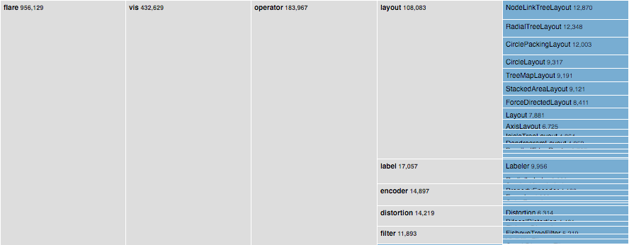
5 | [Examples](https://observablehq.com/@d3/icicle/2?intent=fork) · The partition layout produces adjacency diagrams: a space-filling variant of a [node-link tree diagram](./tree.md). Rather than drawing a link between parent and child in the hierarchy, nodes are drawn as solid areas (either arcs or rectangles), and their placement relative to other nodes reveals their position in the hierarchy. The size of the nodes encodes a quantitative dimension that would be difficult to show in a node-link diagram.
6 |
7 | ## partition() {#partition}
8 |
9 | [Source](https://github.com/d3/d3-hierarchy/blob/main/src/partition.js) · Creates a new partition layout with the default settings.
10 |
11 | ## *partition*(*root*) {#_partition}
12 |
13 | [Source](https://github.com/d3/d3-hierarchy/blob/main/src/partition.js) · Lays out the specified *root* [hierarchy](./hierarchy.md), assigning the following properties on *root* and its descendants:
14 |
15 | * *node*.x0 - the left edge of the rectangle
16 | * *node*.y0 - the top edge of the rectangle
17 | * *node*.x1 - the right edge of the rectangle
18 | * *node*.y1 - the bottom edge of the rectangle
19 |
20 | You must call [*root*.sum](./hierarchy.md#node_sum) before passing the hierarchy to the partition layout. You probably also want to call [*root*.sort](./hierarchy.md#node_sort) to order the hierarchy before computing the layout.
21 |
22 | ## *partition*.size(*size*) {#partition_size}
23 |
24 | [Source](https://github.com/d3/d3-hierarchy/blob/main/src/partition.js) · If *size* is specified, sets this partition layout’s size to the specified two-element array of numbers [*width*, *height*] and returns this partition layout. If *size* is not specified, returns the current size, which defaults to [1, 1].
25 |
26 | ## *partition*.round(*round*) {#partition_round}
27 |
28 | [Source](https://github.com/d3/d3-hierarchy/blob/main/src/partition.js) · If *round* is specified, enables or disables rounding according to the given boolean and returns this partition layout. If *round* is not specified, returns the current rounding state, which defaults to false.
29 |
30 | ## *partition*.padding(*padding*) {#partition_padding}
31 |
32 | [Source](https://github.com/d3/d3-hierarchy/blob/main/src/partition.js) · If *padding* is specified, sets the padding to the specified number and returns this partition layout. If *padding* is not specified, returns the current padding, which defaults to zero. The padding is used to separate a node’s adjacent children.
33 |
--------------------------------------------------------------------------------
/docs/components/ExampleAnimatedQuadtree.vue:
--------------------------------------------------------------------------------
1 |
7 |
53 |
54 |
](https://observablehq.com/@d3/icicle/2?intent=fork)
4 |
5 | [Examples](https://observablehq.com/@d3/icicle/2?intent=fork) · The partition layout produces adjacency diagrams: a space-filling variant of a [node-link tree diagram](./tree.md). Rather than drawing a link between parent and child in the hierarchy, nodes are drawn as solid areas (either arcs or rectangles), and their placement relative to other nodes reveals their position in the hierarchy. The size of the nodes encodes a quantitative dimension that would be difficult to show in a node-link diagram.
6 |
7 | ## partition() {#partition}
8 |
9 | [Source](https://github.com/d3/d3-hierarchy/blob/main/src/partition.js) · Creates a new partition layout with the default settings.
10 |
11 | ## *partition*(*root*) {#_partition}
12 |
13 | [Source](https://github.com/d3/d3-hierarchy/blob/main/src/partition.js) · Lays out the specified *root* [hierarchy](./hierarchy.md), assigning the following properties on *root* and its descendants:
14 |
15 | * *node*.x0 - the left edge of the rectangle
16 | * *node*.y0 - the top edge of the rectangle
17 | * *node*.x1 - the right edge of the rectangle
18 | * *node*.y1 - the bottom edge of the rectangle
19 |
20 | You must call [*root*.sum](./hierarchy.md#node_sum) before passing the hierarchy to the partition layout. You probably also want to call [*root*.sort](./hierarchy.md#node_sort) to order the hierarchy before computing the layout.
21 |
22 | ## *partition*.size(*size*) {#partition_size}
23 |
24 | [Source](https://github.com/d3/d3-hierarchy/blob/main/src/partition.js) · If *size* is specified, sets this partition layout’s size to the specified two-element array of numbers [*width*, *height*] and returns this partition layout. If *size* is not specified, returns the current size, which defaults to [1, 1].
25 |
26 | ## *partition*.round(*round*) {#partition_round}
27 |
28 | [Source](https://github.com/d3/d3-hierarchy/blob/main/src/partition.js) · If *round* is specified, enables or disables rounding according to the given boolean and returns this partition layout. If *round* is not specified, returns the current rounding state, which defaults to false.
29 |
30 | ## *partition*.padding(*padding*) {#partition_padding}
31 |
32 | [Source](https://github.com/d3/d3-hierarchy/blob/main/src/partition.js) · If *padding* is specified, sets the padding to the specified number and returns this partition layout. If *padding* is not specified, returns the current padding, which defaults to zero. The padding is used to separate a node’s adjacent children.
33 |
--------------------------------------------------------------------------------
/docs/components/ExampleAnimatedQuadtree.vue:
--------------------------------------------------------------------------------
1 |
7 |
53 |
54 | 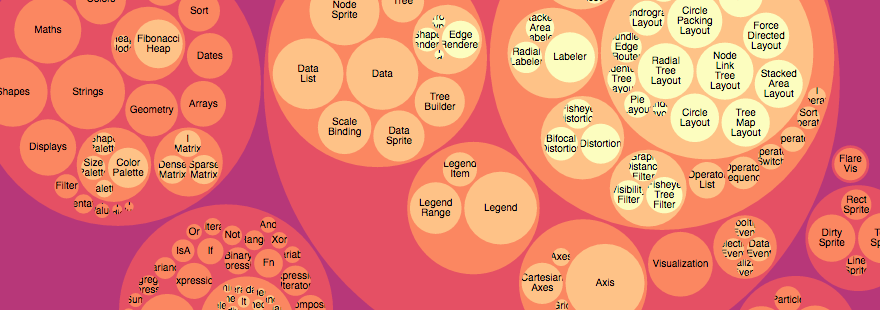 ](https://observablehq.com/@d3/circle-packing)
4 |
5 | [Examples](https://observablehq.com/@d3/circle-packing) · Enclosure diagrams use containment (nesting) to represent a hierarchy. The size of the leaf circles encodes a quantitative dimension of the data. The enclosing circles show the approximate cumulative size of each subtree, but due to wasted space there is some distortion; only the leaf nodes can be compared accurately. Although [circle packing](http://en.wikipedia.org/wiki/Circle_packing) does not use space as efficiently as a [treemap](./treemap.md), the “wasted” space more prominently reveals the hierarchical structure.
6 |
7 | ## pack() {#pack}
8 |
9 | [Source](https://github.com/d3/d3-hierarchy/blob/main/src/pack/index.js) · Creates a new pack layout with the default settings.
10 |
11 | ### *pack*(*root*) {#_pack}
12 |
13 | [Source](https://github.com/d3/d3-hierarchy/blob/main/src/pack/index.js) · Lays out the specified *root* [hierarchy](./hierarchy.md), assigning the following properties on *root* and its descendants:
14 |
15 | * *node*.x - the *x*-coordinate of the circle’s center
16 | * *node*.y - the y coordinate of the circle’s center
17 | * *node*.r - the radius of the circle
18 |
19 | You must call [*root*.sum](./hierarchy.md#node_sum) before passing the hierarchy to the pack layout. You probably also want to call [*root*.sort](./hierarchy.md#node_sort) to order the hierarchy before computing the layout.
20 |
21 | ## *pack*.radius(*radius*) {#pack_radius}
22 |
23 | [Source](https://github.com/d3/d3-hierarchy/blob/main/src/pack/index.js) · If *radius* is specified, sets the pack layout’s radius accessor to the specified function and returns this pack layout. If *radius* is not specified, returns the current radius accessor, which defaults to null. If the radius accessor is null, the radius of each leaf circle is derived from the leaf *node*.value (computed by [*node*.sum](./hierarchy.md#node_sum)); the radii are then scaled proportionally to fit the [layout size](#pack_size). If the radius accessor is not null, the radius of each leaf circle is specified exactly by the function.
24 |
25 | ## *pack*.size(*size*) {#pack_size}
26 |
27 | [Source](https://github.com/d3/d3-hierarchy/blob/main/src/pack/index.js) · If *size* is specified, sets this pack layout’s size to the specified two-element array of numbers [*width*, *height*] and returns this pack layout. If *size* is not specified, returns the current size, which defaults to [1, 1].
28 |
29 | ## *pack*.padding(*padding*) {#pack_padding}
30 |
31 | [Source](https://github.com/d3/d3-hierarchy/blob/main/src/pack/index.js) · If *padding* is specified, sets this pack layout’s padding accessor to the specified number or function and returns this pack layout. If *padding* is not specified, returns the current padding accessor, which defaults to the constant zero. When siblings are packed, tangent siblings will be separated by approximately the specified padding; the enclosing parent circle will also be separated from its children by approximately the specified padding. If an [explicit radius](#pack_radius) is not specified, the padding is approximate because a two-pass algorithm is needed to fit within the [layout size](#pack_size): the circles are first packed without padding; a scaling factor is computed and applied to the specified padding; and lastly the circles are re-packed with padding.
32 |
33 | ## packSiblings(*circles*) {#packSiblings}
34 |
35 | [Source](https://github.com/d3/d3-hierarchy/blob/main/src/pack/siblings.js) · Packs the specified array of *circles*, each of which must have a *circle*.r property specifying the circle’s radius. Assigns the following properties to each circle:
36 |
37 | * *circle*.x - the *x*-coordinate of the circle’s center
38 | * *circle*.y - the y coordinate of the circle’s center
39 |
40 | The circles are positioned according to the front-chain packing algorithm by [Wang *et al.*](https://dl.acm.org/citation.cfm?id=1124851)
41 |
42 | ## packEnclose(*circles*) {#packEnclose}
43 |
44 | [Examples](https://observablehq.com/@d3/d3-packenclose) · [Source](https://github.com/d3/d3-hierarchy/blob/main/src/pack/enclose.js) · Computes the [smallest circle](https://en.wikipedia.org/wiki/Smallest-circle_problem) that encloses the specified array of *circles*, each of which must have a *circle*.r property specifying the circle’s radius, and *circle*.x and *circle*.y properties specifying the circle’s center. The enclosing circle is computed using the [Matoušek-Sharir-Welzl algorithm](http://www.inf.ethz.ch/personal/emo/PublFiles/SubexLinProg_ALG16_96.pdf). (See also [Apollonius’ Problem](https://observablehq.com/@d3/apollonius-problem).)
45 |
--------------------------------------------------------------------------------
/docs/d3-scale/threshold.md:
--------------------------------------------------------------------------------
1 | # Threshold scales
2 |
3 | Threshold scales are similar to [quantize scales](./quantize.md), except they allow you to map arbitrary subsets of the domain to discrete values in the range. The input domain is still continuous, and divided into slices based on a set of threshold values. See [this choropleth](https://observablehq.com/@d3/threshold-choropleth) for an example.
4 |
5 | ## scaleThreshold(*domain*, *range*) {#scaleThreshold}
6 |
7 | [Examples](https://observablehq.com/@d3/quantile-quantize-and-threshold-scales) · [Source](https://github.com/d3/d3-scale/blob/main/src/threshold.js) · Constructs a new threshold scale with the specified [*domain*](#threshold_domain) and [*range*](#threshold_range).
8 |
9 | ```js
10 | const color = d3.scaleThreshold([0, 1], ["red", "white", "blue"]);
11 | ```
12 |
13 | If *domain* is not specified, it defaults to [0.5].
14 |
15 | ```js
16 | const color = d3.scaleThreshold(["red", "blue"]);
17 | color(0); // "red"
18 | color(1); // "blue"
19 | ```
20 |
21 | If *range* is not specified, it defaults to [0, 1].
22 |
23 | ## *threshold*(*value*) {#_threshold}
24 |
25 | [Examples](https://observablehq.com/@d3/quantile-quantize-and-threshold-scales) · [Source](https://github.com/d3/d3-scale/blob/main/src/threshold.js) · Given a *value* in the input [domain](#threshold_domain), returns the corresponding value in the output [range](#threshold_range). For example:
26 |
27 | ```js
28 | const color = d3.scaleThreshold([0, 1], ["red", "white", "green"]);
29 | color(-1); // "red"
30 | color(0); // "white"
31 | color(0.5); // "white"
32 | color(1); // "green"
33 | color(1000); // "green"
34 | ```
35 |
36 | ## *threshold*.invertExtent(*value*) {#threshold_invertExtent}
37 |
38 | [Source](https://github.com/d3/d3-scale/blob/main/src/threshold.js) · Returns the extent of values in the [domain](#threshold_domain) [x0, x1] for the corresponding *value* in the [range](#threshold_range), representing the inverse mapping from range to domain.
39 |
40 | ```js
41 | const color = d3.scaleThreshold([0, 1], ["red", "white", "green"]);
42 | color.invertExtent("red"); // [undefined, 0]
43 | color.invertExtent("white"); // [0, 1]
44 | color.invertExtent("green"); // [1, undefined]
45 | ```
46 |
47 | This method is useful for interaction, say to determine the value in the domain that corresponds to the pixel location under the mouse. The extent below the lowest threshold is undefined (unbounded), as is the extent above the highest threshold.
48 |
49 | ## *threshold*.domain(*domain*) {#threshold_domain}
50 |
51 | [Examples](https://observablehq.com/@d3/quantile-quantize-and-threshold-scales) · [Source](https://github.com/d3/d3-scale/blob/main/src/threshold.js) · If *domain* is specified, sets the scale’s domain to the specified array of values.
52 |
53 | ```js
54 | const color = d3.scaleThreshold(["red", "white", "green"]).domain([0, 1]);
55 | ```
56 |
57 | The values must be in ascending order or the behavior of the scale is undefined. The values are typically numbers, but any naturally ordered values (such as strings) will work; a threshold scale can be used to encode any type that is ordered. If the number of values in the scale’s range is *n* + 1, the number of values in the scale’s domain must be *n*. If there are fewer than *n* elements in the domain, the additional values in the range are ignored. If there are more than *n* elements in the domain, the scale may return undefined for some inputs.
58 |
59 | If *domain* is not specified, returns the scale’s current domain.
60 |
61 | ```js
62 | color.domain() // [0, 1]
63 | ```
64 |
65 | ## *threshold*.range(*range*) {#threshold_range}
66 |
67 | [Examples](https://observablehq.com/@d3/quantile-quantize-and-threshold-scales) · [Source](https://github.com/d3/d3-scale/blob/main/src/threshold.js) · If *range* is specified, sets the scale’s range to the specified array of values.
68 |
69 | ```js
70 | const color = d3.scaleThreshold().range(["red", "white", "green"]);
71 | ```
72 |
73 | If the number of values in the scale’s domain is *n*, the number of values in the scale’s range must be *n* + 1. If there are fewer than *n* + 1 elements in the range, the scale may return undefined for some inputs. If there are more than *n* + 1 elements in the range, the additional values are ignored. The elements in the given array need not be numbers; any value or type will work.
74 |
75 | If *range* is not specified, returns the scale’s current range.
76 |
77 | ```js
78 | color.range() // ["red", "white", "green"]
79 | ```
80 |
81 | ## *threshold*.copy() {#threshold_copy}
82 |
83 | [Examples](https://observablehq.com/@d3/quantile-quantize-and-threshold-scales) · [Source](https://github.com/d3/d3-scale/blob/main/src/threshold.js) · Returns an exact copy of this scale.
84 |
85 | ```js
86 | const c1 = d3.scaleThreshold(d3.schemeBlues[5]);
87 | const c2 = c1.copy();
88 | ```
89 |
90 | Changes to this scale will not affect the returned scale, and vice versa.
91 |
--------------------------------------------------------------------------------
/docs/d3-chord/chord.md:
--------------------------------------------------------------------------------
1 | # Chords
2 |
3 | The chord layout computes angles to generate a [chord diagram](../d3-chord.md).
4 |
5 | ## chord() {#chord}
6 |
7 | [Source](https://github.com/d3/d3-chord/blob/main/src/chord.js) · Constructs a new chord layout with the default settings.
8 |
9 | ```js
10 | const chord = d3.chord();
11 | ```
12 |
13 | ## *chord*(*matrix*) {#_chord}
14 |
15 | [Source](https://github.com/d3/d3-chord/blob/main/src/chord.js) · Computes the chord layout for the specified square *matrix* of size *n*×*n*, where the *matrix* represents the directed flow amongst a network (a complete digraph) of *n* nodes.
16 |
17 | The return value of *chord*(*matrix*) is an array of *chords*, where each chord represents the combined bidirectional flow between two nodes *i* and *j* (where *i* may be equal to *j*) and is an object with the following properties:
18 |
19 | * `source` - the source subgroup
20 | * `target` - the target subgroup
21 |
22 | Each source and target subgroup is also an object with the following properties:
23 |
24 | * `startAngle` - the start angle in radians
25 | * `endAngle` - the end angle in radians
26 | * `value` - the flow value *matrix*[*i*][*j*]
27 | * `index` - the node index *i*
28 |
29 | The chords are typically passed to [ribbon](./ribbon.md) to display the network relationships.
30 |
31 | The returned array includes only chord objects for which the value *matrix*[*i*][*j*] or *matrix*[*j*][*i*] is non-zero. Furthermore, the returned array only contains unique chords: a given chord *ij* represents the bidirectional flow from *i* to *j* *and* from *j* to *i*, and does not contain a duplicate chord *ji*; *i* and *j* are chosen such that the chord’s source always represents the larger of *matrix*[*i*][*j*] and *matrix*[*j*][*i*].
32 |
33 | The *chords* array also defines a secondary array of length *n*, *chords*.groups, where each group represents the combined outflow for node *i*, corresponding to the elements *matrix*[*i*][0 … *n* - 1], and is an object with the following properties:
34 |
35 | * `startAngle` - the start angle in radians
36 | * `endAngle` - the end angle in radians
37 | * `value` - the total outgoing flow value for node *i*
38 | * `index` - the node index *i*
39 |
40 | The groups are typically passed to [arc](../d3-shape/arc.md) to produce a donut chart around the circumference of the chord layout.
41 |
42 | ## *chord*.padAngle(*angle*) {#chord_padAngle}
43 |
44 | [Source](https://github.com/d3/d3-chord/blob/main/src/chord.js) · If *angle* is specified, sets the pad angle between adjacent groups to the specified number in radians and returns this chord layout. If *angle* is not specified, returns the current pad angle, which defaults to zero.
45 |
46 | ## *chord*.sortGroups(*compare*) {#chord_sortGroups}
47 |
48 | [Source](https://github.com/d3/d3-chord/blob/main/src/chord.js) · If *compare* is specified, sets the group comparator to the specified function or null and returns this chord layout. If *compare* is not specified, returns the current group comparator, which defaults to null. If the group comparator is non-null, it is used to sort the groups by their total outflow. See also [ascending](../d3-array/sort.md#ascending) and [descending](../d3-array/sort.md#descending).
49 |
50 | ## *chord*.sortSubgroups(*compare*) {#chord_sortSubgroups}
51 |
52 | [Source](https://github.com/d3/d3-chord/blob/main/src/chord.js) · If *compare* is specified, sets the subgroup comparator to the specified function or null and returns this chord layout. If *compare* is not specified, returns the current subgroup comparator, which defaults to null. If the subgroup comparator is non-null, it is used to sort the subgroups corresponding to *matrix*[*i*][0 … *n* - 1] for a given group *i* by their total outflow. See also [ascending](../d3-array/sort.md#ascending) and [descending](../d3-array/sort.md#descending).
53 |
54 | ## *chord*.sortChords(*compare*) {#chord_sortChords}
55 |
56 | [Source](https://github.com/d3/d3-chord/blob/main/src/chord.js) · If *compare* is specified, sets the chord comparator to the specified function or null and returns this chord layout. If *compare* is not specified, returns the current chord comparator, which defaults to null. If the chord comparator is non-null, it is used to sort the [chords](#_chord) by their combined flow; this only affects the *z*-order of the chords. See also [ascending](../d3-array/sort.md#ascending) and [descending](../d3-array/sort.md#descending).
57 |
58 | ## chordDirected() {#chordDirected}
59 |
60 | [Examples](https://observablehq.com/@d3/directed-chord-diagram) · [Source](https://github.com/d3/d3-chord/blob/main/src/chord.js) · A chord layout for unidirectional flows. The chord from *i* to *j* is generated from the value in *matrix*[*i*][*j*] only.
61 |
62 | ## chordTranspose() {#chordTranspose}
63 |
64 | [Source](https://github.com/d3/d3-chord/blob/main/src/chord.js) · A transposed chord layout. Useful to highlight outgoing (rather than incoming) flows.
65 |
--------------------------------------------------------------------------------
/docs/d3-array/ticks.md:
--------------------------------------------------------------------------------
1 | # Ticks {#Ticks}
2 |
3 | Generate representative values from a continuous interval.
4 |
5 | ## ticks(*start*, *stop*, *count*) {#ticks}
6 |
7 | [Examples](https://observablehq.com/@d3/d3-ticks) · [Source](https://github.com/d3/d3-array/blob/main/src/ticks.js) · Returns an array of approximately *count* + 1 uniformly-spaced, nicely-rounded values between *start* and *stop* (inclusive). Each value is a power of ten multiplied by 1, 2 or 5.
8 |
9 | ```js
10 | d3.ticks(1, 9, 5) // [2, 4, 6, 8]
11 | ```
12 | ```js
13 | d3.ticks(1, 9, 20) // [1, 1.5, 2, 2.5, 3, 3.5, 4, 4.5, 5, 5.5, 6, 6.5, 7, 7.5, 8, 8.5, 9]
14 | ```
15 |
16 | Ticks are inclusive in the sense that they may include the specified *start* and *stop* values if (and only if) they are exact, nicely-rounded values consistent with the inferred [step](#tickStep). More formally, each returned tick *t* satisfies *start* ≤ *t* and *t* ≤ *stop*.
17 |
18 | ## tickIncrement(*start*, *stop*, *count*) {#tickIncrement}
19 |
20 | [Source](https://github.com/d3/d3-array/blob/main/src/ticks.js) · Like [d3.tickStep](#tickStep), except requires that *start* is always less than or equal to *stop*, and if the tick step for the given *start*, *stop* and *count* would be less than one, returns the negative inverse tick step instead.
21 |
22 | ```js
23 | d3.tickIncrement(1, 9, 5) // 2
24 | ```
25 | ```js
26 | d3.tickIncrement(1, 9, 20) // -2, meaning a tick step 0.5
27 | ```
28 |
29 | This method is always guaranteed to return an integer, and is used by [d3.ticks](#ticks) to guarantee that the returned tick values are represented as precisely as possible in IEEE 754 floating point.
30 |
31 | ## tickStep(*start*, *stop*, *count*) {#tickStep}
32 |
33 | [Source](https://github.com/d3/d3-array/blob/main/src/ticks.js) · Returns the difference between adjacent tick values if the same arguments were passed to [d3.ticks](#ticks): a nicely-rounded value that is a power of ten multiplied by 1, 2 or 5.
34 |
35 | ```js
36 | d3.tickStep(1, 9, 5) // 2
37 | ```
38 |
39 | If *stop* is less than *start*, may return a negative tick step to indicate descending ticks.
40 |
41 | ```js
42 | d3.tickStep(9, 1, 5) // -2
43 | ```
44 |
45 | Note that due to the limited precision of IEEE 754 floating point, the returned value may not be exact decimals; use [d3-format](../d3-format.md) to format numbers for human consumption.
46 |
47 | ## nice(*start*, *stop*, *count*) {#nice}
48 |
49 | [Source](https://github.com/d3/d3-array/blob/main/src/nice.js) · Returns a new interval [*niceStart*, *niceStop*] covering the given interval [*start*, *stop*] and where *niceStart* and *niceStop* are guaranteed to align with the corresponding [tick step](#tickStep).
50 |
51 | ```js
52 | d3.nice(1, 9, 5) // [0, 10]
53 | ```
54 |
55 | Like [d3.tickIncrement](#tickIncrement), this requires that *start* is less than or equal to *stop*.
56 |
57 | ## range(*start*, *stop*, *step*) {#range}
58 |
59 | [Examples](https://observablehq.com/@d3/d3-range) · [Source](https://github.com/d3/d3-array/blob/main/src/range.js) · Returns an array containing an arithmetic progression, similar to the Python built-in [range](http://docs.python.org/library/functions.html#range). This method is often used to iterate over a sequence of uniformly-spaced numeric values, such as the indexes of an array or the ticks of a linear scale. (See also [d3.ticks](#ticks) for nicely-rounded values.)
60 |
61 | ```js
62 | d3.range(6) // [0, 1, 2, 3, 4, 5]
63 | ```
64 |
65 | If *step* is omitted, it defaults to 1. If *start* is omitted, it defaults to 0. The *stop* value is exclusive; it is not included in the result. If *step* is positive, the last element is the largest *start* + *i* \* *step* less than *stop*; if *step* is negative, the last element is the smallest *start* + *i* \* *step* greater than *stop*.
66 |
67 | ```js
68 | d3.range(5, -1, -1) // [5, 4, 3, 2, 1, 0]
69 | ```
70 |
71 | If the returned array would contain an infinite number of values, an empty range is returned.
72 |
73 | ```js
74 | d3.range(Infinity) // []
75 | ```
76 |
77 | The arguments are not required to be integers; however, the results are more predictable if they are. The values in the returned array are defined as *start* + *i* \* *step*, where *i* is an integer from zero to one minus the total number of elements in the returned array.
78 |
79 | ```js
80 | d3.range(0, 1, 0.2) // [0, 0.2, 0.4, 0.6000000000000001, 0.8]
81 | ```
82 |
83 | This behavior is due to IEEE 754 double-precision floating point, which defines 0.2 * 3 = 0.6000000000000001. Use [d3-format](../d3-format.md) to format numbers for human consumption with appropriate rounding; see also [*linear*.tickFormat](../d3-scale/linear.md#linear_tickFormat) in [d3-scale](../d3-scale.md). Likewise, if the returned array should have a specific length, consider using [*array*.map](https://developer.mozilla.org/docs/Web/JavaScript/Reference/Global_Objects/Array/map) on an integer range.
84 |
85 | ```js
86 | d3.range(0, 1, 1 / 49) // 👎 returns 50 elements!
87 | ```
88 | ```js
89 | d3.range(49).map((d) => d / 49) // 👍 returns 49 elements
90 | ```
91 |
--------------------------------------------------------------------------------
/docs/d3-scale/quantize.md:
--------------------------------------------------------------------------------
1 | # Quantize scales
2 |
3 | Quantize scales are similar to [linear scales](./linear.md), except they use a discrete rather than continuous range. The continuous input domain is divided into uniform segments based on the number of values in (*i.e.*, the cardinality of) the output range. Each range value *y* can be expressed as a quantized linear function of the domain value *x*: *y* = *m round(x)* + *b*. See [the quantized choropleth](https://observablehq.com/@d3/choropleth/2?intent=fork) for an example.
4 |
5 | ## scaleQuantize(*domain*, *range*) {#scaleQuantize}
6 |
7 | [Examples](https://observablehq.com/@d3/quantile-quantize-and-threshold-scales) · [Source](https://github.com/d3/d3-scale/blob/main/src/quantize.js) · Constructs a new quantize scale with the specified [*domain*](#quantize_domain) and [*range*](#quantize_range).
8 |
9 | ```js
10 | const color = d3.scaleQuantize([0, 100], d3.schemeBlues[9]);
11 | ```
12 |
13 | If either *domain* or *range* is not specified, each defaults to [0, 1].
14 |
15 | ```js
16 | const color = d3.scaleQuantize(d3.schemeBlues[9]);
17 | ```
18 |
19 | ## *quantize*(*value*) {#_quantize}
20 |
21 | [Examples](https://observablehq.com/@d3/quantile-quantize-and-threshold-scales) · [Source](https://github.com/d3/d3-scale/blob/main/src/quantize.js) · Given a *value* in the input [domain](#quantize_domain), returns the corresponding value in the output [range](#quantize_range). For example, to apply a color encoding:
22 |
23 | ```js
24 | const color = d3.scaleQuantize([0, 1], ["brown", "steelblue"]);
25 | color(0.49); // "brown"
26 | color(0.51); // "steelblue"
27 | ```
28 |
29 | Or dividing the domain into three equally-sized parts with different range values to compute an appropriate stroke width:
30 |
31 | ```js
32 | const width = d3.scaleQuantize([10, 100], [1, 2, 4]);
33 | width(20); // 1
34 | width(50); // 2
35 | width(80); // 4
36 | ```
37 |
38 | ## *quantize*.invertExtent(*value*) {#quantize_invertExtent}
39 |
40 | [Examples](https://observablehq.com/@d3/quantile-quantize-and-threshold-scales) · [Source](https://github.com/d3/d3-scale/blob/main/src/quantize.js) · Returns the extent of values in the [domain](#quantize_domain) [x0, x1] for the corresponding *value* in the [range](#quantize_range): the inverse of [*quantize*](#_quantize). This method is useful for interaction, say to determine the value in the domain that corresponds to the pixel location under the mouse.
41 |
42 | ```js
43 | const width = d3.scaleQuantize([10, 100], [1, 2, 4]);
44 | width.invertExtent(2); // [40, 70]
45 | ```
46 |
47 | ## *quantize*.domain(*domain*) {#quantize_domain}
48 |
49 | [Examples](https://observablehq.com/@d3/quantile-quantize-and-threshold-scales) · [Source](https://github.com/d3/d3-scale/blob/main/src/quantize.js) · If *domain* is specified, sets the scale’s domain to the specified two-element array of numbers.
50 |
51 | ```js
52 | const color = d3.scaleQuantize(d3.schemeBlues[9]);
53 | color.domain([0, 100]);
54 | ```
55 |
56 | If the elements in the given array are not numbers, they will be coerced to numbers. The numbers must be in ascending order or the behavior of the scale is undefined.
57 |
58 | If *domain* is not specified, returns the scale’s current domain.
59 |
60 | ```js
61 | color.domain() // [0, 100]
62 | ```
63 |
64 | ## *quantize*.range(*range*) {#quantize_range}
65 |
66 | [Examples](https://observablehq.com/@d3/quantile-quantize-and-threshold-scales) · [Source](https://github.com/d3/d3-scale/blob/main/src/quantize.js) · If *range* is specified, sets the scale’s range to the specified array of values.
67 |
68 | ```js
69 | const color = d3.scaleQuantize();
70 | color.range(d3.schemeBlues[5]);
71 | ```
72 |
73 | The array may contain any number of discrete values. The elements in the given array need not be numbers; any value or type will work.
74 |
75 | If *range* is not specified, returns the scale’s current range.
76 |
77 | ```js
78 | color.range() // ["#eff3ff", "#bdd7e7", "#6baed6", "#3182bd", "#08519c"]
79 | ```
80 |
81 | ## *quantize*.thresholds() {#quantize_thresholds}
82 |
83 | [Examples](https://observablehq.com/@d3/quantile-quantize-and-threshold-scales) · [Source](https://github.com/d3/d3-scale/blob/main/src/quantize.js) · Returns the array of computed thresholds within the [domain](#quantize_domain).
84 |
85 | ```js
86 | color.thresholds() // [0.2, 0.4, 0.6, 0.8]
87 | ```
88 |
89 | The number of returned thresholds is one less than the length of the [range](#quantize_range): values less than the first threshold are assigned the first element in the range, whereas values greater than or equal to the last threshold are assigned the last element in the range.
90 |
91 | ## *quantize*.copy() {#quantize_copy}
92 |
93 | [Examples](https://observablehq.com/@d3/quantile-quantize-and-threshold-scales) · [Source](https://github.com/d3/d3-scale/blob/main/src/quantize.js) · Returns an exact copy of this scale.
94 |
95 | ```js
96 | const c1 = d3.scaleQuantize(d3.schemeBlues[5]);
97 | const c2 = c1.copy();
98 | ```
99 |
100 | Changes to this scale will not affect the returned scale, and vice versa.
101 |
--------------------------------------------------------------------------------
/docs/d3-hierarchy/stratify.md:
--------------------------------------------------------------------------------
1 | # Stratify {#Stratify}
2 |
3 | [Examples](https://observablehq.com/@d3/d3-stratify) · Consider the following table of relationships:
4 |
5 | Name | Parent
6 | ------|--------
7 | Eve |
8 | Cain | Eve
9 | Seth | Eve
10 | Enos | Seth
11 | Noam | Seth
12 | Abel | Eve
13 | Awan | Eve
14 | Enoch | Awan
15 | Azura | Eve
16 |
17 | These names are conveniently unique, so we can unambiguously represent the hierarchy as a CSV file:
18 |
19 | ```
20 | name,parent
21 | Eve,
22 | Cain,Eve
23 | Seth,Eve
24 | Enos,Seth
25 | Noam,Seth
26 | Abel,Eve
27 | Awan,Eve
28 | Enoch,Awan
29 | Azura,Eve
30 | ```
31 |
32 | To parse the CSV using [csvParse](../d3-dsv.md#csvParse):
33 |
34 | ```js
35 | const table = d3.csvParse(text);
36 | ```
37 |
38 | This returns an array of {*name*, *parent*} objects:
39 |
40 | ```json
41 | [
42 | {"name": "Eve", "parent": ""},
43 | {"name": "Cain", "parent": "Eve"},
44 | {"name": "Seth", "parent": "Eve"},
45 | {"name": "Enos", "parent": "Seth"},
46 | {"name": "Noam", "parent": "Seth"},
47 | {"name": "Abel", "parent": "Eve"},
48 | {"name": "Awan", "parent": "Eve"},
49 | {"name": "Enoch", "parent": "Awan"},
50 | {"name": "Azura", "parent": "Eve"}
51 | ]
52 | ```
53 |
54 | To convert to a [hierarchy](./hierarchy.md):
55 |
56 | ```js
57 | const root = d3.stratify()
58 | .id((d) => d.name)
59 | .parentId((d) => d.parent)
60 | (table);
61 | ```
62 |
63 | This hierarchy can now be passed to a hierarchical layout, such as [tree](./tree.md), for visualization.
64 |
65 | The stratify operator also works with [delimited paths](#stratify_path) as is common in file systems.
66 |
67 | ## stratify() {#stratify}
68 |
69 | [Source](https://github.com/d3/d3-hierarchy/blob/main/src/stratify.js) · Constructs a new stratify operator with the default settings.
70 |
71 | ```js
72 | const stratify = d3.stratify();
73 | ```
74 |
75 | ## *stratify*(*data*) {#_stratify}
76 |
77 | [Source](https://github.com/d3/d3-hierarchy/blob/main/src/stratify.js) · Generates a new hierarchy from the specified tabular *data*.
78 |
79 | ```js
80 | const root = stratify(data);
81 | ```
82 |
83 | ## *stratify*.id(*id*) {#stratify_id}
84 |
85 | [Source](https://github.com/d3/d3-hierarchy/blob/main/src/stratify.js) · If *id* is specified, sets the id accessor to the given function and returns this stratify operator. Otherwise, returns the current id accessor, which defaults to:
86 |
87 | ```js
88 | function id(d) {
89 | return d.id;
90 | }
91 | ```
92 |
93 | The id accessor is invoked for each element in the input data passed to the [stratify operator](#_stratify), being passed the current datum (*d*) and the current index (*i*). The returned string is then used to identify the node’s relationships in conjunction with the [parent id](#stratify_parentId). For leaf nodes, the id may be undefined; otherwise, the id must be unique. (Null and the empty string are equivalent to undefined.)
94 |
95 | ## *stratify*.parentId(*parentId*) {#stratify_parentId}
96 |
97 | [Source](https://github.com/d3/d3-hierarchy/blob/main/src/stratify.js) · If *parentId* is specified, sets the parent id accessor to the given function and returns this stratify operator. Otherwise, returns the current parent id accessor, which defaults to:
98 |
99 | ```js
100 | function parentId(d) {
101 | return d.parentId;
102 | }
103 | ```
104 |
105 | The parent id accessor is invoked for each element in the input data passed to the [stratify operator](#_stratify), being passed the current datum (*d*) and the current index (*i*). The returned string is then used to identify the node’s relationships in conjunction with the [id](#stratify_id). For the root node, the parent id should be undefined. (Null and the empty string are equivalent to undefined.) There must be exactly one root node in the input data, and no circular relationships.
106 |
107 | ## *stratify*.path(*path*) {#stratify_path}
108 |
109 | [Source](https://github.com/d3/d3-hierarchy/blob/main/src/stratify.js) · If *path* is specified, sets the path accessor to the given function and returns this stratify operator. Otherwise, returns the current path accessor, which defaults to undefined.
110 |
111 | If a path accessor is set, the [id](#stratify_id) and [parentId](#stratify_parentId) accessors are ignored, and a unix-like hierarchy is computed on the slash-delimited strings returned by the path accessor, imputing parent nodes and ids as necessary.
112 |
113 | For example, given the output of the UNIX find command in the local directory:
114 |
115 | ```js
116 | const paths = [
117 | "axes.js",
118 | "channel.js",
119 | "context.js",
120 | "legends.js",
121 | "legends/ramp.js",
122 | "marks/density.js",
123 | "marks/dot.js",
124 | "marks/frame.js",
125 | "scales/diverging.js",
126 | "scales/index.js",
127 | "scales/ordinal.js",
128 | "stats.js",
129 | "style.js",
130 | "transforms/basic.js",
131 | "transforms/bin.js",
132 | "transforms/centroid.js",
133 | "warnings.js",
134 | ];
135 | ```
136 |
137 | You can say:
138 |
139 | ```js
140 | const root = d3.stratify().path((d) => d)(paths);
141 | ```
142 |
--------------------------------------------------------------------------------
/docs/d3-scale/log.md:
--------------------------------------------------------------------------------
1 | # Logarithmic scales
2 |
3 | Logarithmic (“log”) scales are like [linear scales](./linear.md) except that a logarithmic transform is applied to the input domain value before the output range value is computed. The mapping to the range value *y* can be expressed as a function of the domain value *x*: *y* = *m* log(x) + *b*.
4 |
5 | :::warning CAUTION
6 | As log(0) = -∞, a log scale domain must be **strictly-positive or strictly-negative**; the domain must not include or cross zero. A log scale with a positive domain has a well-defined behavior for positive values, and a log scale with a negative domain has a well-defined behavior for negative values. (For a negative domain, input and output values are implicitly multiplied by -1.) The behavior of the scale is undefined if you pass a negative value to a log scale with a positive domain or vice versa.
7 | :::
8 |
9 | ## scaleLog(*domain*, *range*) {#scaleLog}
10 |
11 | [Examples](https://observablehq.com/@d3/continuous-scales) · [Source](https://github.com/d3/d3-scale/blob/main/src/log.js) · Constructs a new log scale with the specified [domain](./linear.md#linear_domain) and [range](./linear.md#linear_range), the [base](#log_base) 10, the [default](../d3-interpolate/value.md#interpolate) [interpolator](./linear.md#linear_interpolate) and [clamping](./linear.md#linear_clamp) disabled.
12 |
13 | ```js
14 | const x = d3.scaleLog([1, 10], [0, 960]);
15 | ```
16 |
17 | If *domain* is not specified, it defaults to [1, 10]. If *range* is not specified, it defaults to [0, 1].
18 |
19 | ## *log*.base(*base*) {#log_base}
20 |
21 | [Examples](https://observablehq.com/@d3/continuous-scales) · [Source](https://github.com/d3/d3-scale/blob/main/src/log.js) · If *base* is specified, sets the base for this logarithmic scale to the specified value.
22 |
23 | ```js
24 | const x = d3.scaleLog([1, 1024], [0, 960]).base(2);
25 | ```
26 |
27 | If *base* is not specified, returns the current base, which defaults to 10. Note that due to the nature of a logarithmic transform, the base does not affect the encoding of the scale; it only affects which [ticks](#log_ticks) are chosen.
28 |
29 | ## *log*.ticks(*count*) {#log_ticks}
30 |
31 | [Examples](https://observablehq.com/@d3/scale-ticks) · [Source](https://github.com/d3/d3-scale/blob/main/src/log.js) · Like [*linear*.ticks](./linear.md#linear_ticks), but customized for a log scale.
32 |
33 | ```js
34 | const x = d3.scaleLog([1, 100], [0, 960]);
35 | const T = x.ticks(); // [1, 2, 3, 4, 5, 6, 7, 8, 9, 10, 20, 30, 40, 50, 60, 70, 80, 90, 100]
36 | ```
37 |
38 | If the [base](#log_base) is an integer, the returned ticks are uniformly spaced within each integer power of base; otherwise, one tick per power of base is returned. The returned ticks are guaranteed to be within the extent of the domain. If the orders of magnitude in the [domain](./linear.md#linear_domain) is greater than *count*, then at most one tick per power is returned. Otherwise, the tick values are unfiltered, but note that you can use [*log*.tickFormat](./linear.md#linear_tickFormat) to filter the display of tick labels. If *count* is not specified, it defaults to 10.
39 |
40 | ## *log*.tickFormat(*count*, *specifier*) {#log_tickFormat}
41 |
42 | [Examples](https://observablehq.com/@d3/scale-ticks) · [Source](https://github.com/d3/d3-scale/blob/main/src/log.js) · Like [*linear*.tickFormat](./linear.md#linear_tickFormat), but customized for a log scale. The specified *count* typically has the same value as the count that is used to generate the [tick values](#log_ticks).
43 |
44 | ```js
45 | const x = d3.scaleLog([1, 100], [0, 960]);
46 | const T = x.ticks(); // [1, 2, 3, 4, 5, 6, 7, 8, 9, 10, …]
47 | const f = x.tickFormat();
48 | T.map(f); // ["1", "2", "3", "4", "5", "", "", "", "", "10", …]
49 | ```
50 |
51 | If there are too many ticks, the formatter may return the empty string for some of the tick labels; however, note that the ticks are still shown to convey the logarithmic transform accurately. To disable filtering, specify a *count* of Infinity.
52 |
53 | When specifying a count, you may also provide a format *specifier* or format function. For example, to get a tick formatter that will display 20 ticks of a currency, say `log.tickFormat(20, "$,f")`. If the specifier does not have a defined precision, the precision will be set automatically by the scale, returning the appropriate format. This provides a convenient way of specifying a format whose precision will be automatically set by the scale.
54 |
55 | ## *log*.nice() {#log_nice}
56 |
57 | [Examples](https://observablehq.com/@d3/continuous-scales) · [Source](https://github.com/d3/d3-scale/blob/main/src/log.js) · Like [*linear*.nice](./linear.md#linear_nice), except extends the domain to integer powers of [base](#log_base).
58 |
59 | ```js
60 | const x = d3.scaleLog([0.201479, 0.996679], [0, 960]).nice();
61 | x.domain(); // [0.1, 1]
62 | ```
63 |
64 | If the domain has more than two values, nicing the domain only affects the first and last value. Nicing a scale only modifies the current domain; it does not automatically nice domains that are subsequently set using [*log*.domain](./linear.md#linear_domain). You must re-nice the scale after setting the new domain, if desired.
65 |
66 |
--------------------------------------------------------------------------------
](https://observablehq.com/@d3/circle-packing)
4 |
5 | [Examples](https://observablehq.com/@d3/circle-packing) · Enclosure diagrams use containment (nesting) to represent a hierarchy. The size of the leaf circles encodes a quantitative dimension of the data. The enclosing circles show the approximate cumulative size of each subtree, but due to wasted space there is some distortion; only the leaf nodes can be compared accurately. Although [circle packing](http://en.wikipedia.org/wiki/Circle_packing) does not use space as efficiently as a [treemap](./treemap.md), the “wasted” space more prominently reveals the hierarchical structure.
6 |
7 | ## pack() {#pack}
8 |
9 | [Source](https://github.com/d3/d3-hierarchy/blob/main/src/pack/index.js) · Creates a new pack layout with the default settings.
10 |
11 | ### *pack*(*root*) {#_pack}
12 |
13 | [Source](https://github.com/d3/d3-hierarchy/blob/main/src/pack/index.js) · Lays out the specified *root* [hierarchy](./hierarchy.md), assigning the following properties on *root* and its descendants:
14 |
15 | * *node*.x - the *x*-coordinate of the circle’s center
16 | * *node*.y - the y coordinate of the circle’s center
17 | * *node*.r - the radius of the circle
18 |
19 | You must call [*root*.sum](./hierarchy.md#node_sum) before passing the hierarchy to the pack layout. You probably also want to call [*root*.sort](./hierarchy.md#node_sort) to order the hierarchy before computing the layout.
20 |
21 | ## *pack*.radius(*radius*) {#pack_radius}
22 |
23 | [Source](https://github.com/d3/d3-hierarchy/blob/main/src/pack/index.js) · If *radius* is specified, sets the pack layout’s radius accessor to the specified function and returns this pack layout. If *radius* is not specified, returns the current radius accessor, which defaults to null. If the radius accessor is null, the radius of each leaf circle is derived from the leaf *node*.value (computed by [*node*.sum](./hierarchy.md#node_sum)); the radii are then scaled proportionally to fit the [layout size](#pack_size). If the radius accessor is not null, the radius of each leaf circle is specified exactly by the function.
24 |
25 | ## *pack*.size(*size*) {#pack_size}
26 |
27 | [Source](https://github.com/d3/d3-hierarchy/blob/main/src/pack/index.js) · If *size* is specified, sets this pack layout’s size to the specified two-element array of numbers [*width*, *height*] and returns this pack layout. If *size* is not specified, returns the current size, which defaults to [1, 1].
28 |
29 | ## *pack*.padding(*padding*) {#pack_padding}
30 |
31 | [Source](https://github.com/d3/d3-hierarchy/blob/main/src/pack/index.js) · If *padding* is specified, sets this pack layout’s padding accessor to the specified number or function and returns this pack layout. If *padding* is not specified, returns the current padding accessor, which defaults to the constant zero. When siblings are packed, tangent siblings will be separated by approximately the specified padding; the enclosing parent circle will also be separated from its children by approximately the specified padding. If an [explicit radius](#pack_radius) is not specified, the padding is approximate because a two-pass algorithm is needed to fit within the [layout size](#pack_size): the circles are first packed without padding; a scaling factor is computed and applied to the specified padding; and lastly the circles are re-packed with padding.
32 |
33 | ## packSiblings(*circles*) {#packSiblings}
34 |
35 | [Source](https://github.com/d3/d3-hierarchy/blob/main/src/pack/siblings.js) · Packs the specified array of *circles*, each of which must have a *circle*.r property specifying the circle’s radius. Assigns the following properties to each circle:
36 |
37 | * *circle*.x - the *x*-coordinate of the circle’s center
38 | * *circle*.y - the y coordinate of the circle’s center
39 |
40 | The circles are positioned according to the front-chain packing algorithm by [Wang *et al.*](https://dl.acm.org/citation.cfm?id=1124851)
41 |
42 | ## packEnclose(*circles*) {#packEnclose}
43 |
44 | [Examples](https://observablehq.com/@d3/d3-packenclose) · [Source](https://github.com/d3/d3-hierarchy/blob/main/src/pack/enclose.js) · Computes the [smallest circle](https://en.wikipedia.org/wiki/Smallest-circle_problem) that encloses the specified array of *circles*, each of which must have a *circle*.r property specifying the circle’s radius, and *circle*.x and *circle*.y properties specifying the circle’s center. The enclosing circle is computed using the [Matoušek-Sharir-Welzl algorithm](http://www.inf.ethz.ch/personal/emo/PublFiles/SubexLinProg_ALG16_96.pdf). (See also [Apollonius’ Problem](https://observablehq.com/@d3/apollonius-problem).)
45 |
--------------------------------------------------------------------------------
/docs/d3-scale/threshold.md:
--------------------------------------------------------------------------------
1 | # Threshold scales
2 |
3 | Threshold scales are similar to [quantize scales](./quantize.md), except they allow you to map arbitrary subsets of the domain to discrete values in the range. The input domain is still continuous, and divided into slices based on a set of threshold values. See [this choropleth](https://observablehq.com/@d3/threshold-choropleth) for an example.
4 |
5 | ## scaleThreshold(*domain*, *range*) {#scaleThreshold}
6 |
7 | [Examples](https://observablehq.com/@d3/quantile-quantize-and-threshold-scales) · [Source](https://github.com/d3/d3-scale/blob/main/src/threshold.js) · Constructs a new threshold scale with the specified [*domain*](#threshold_domain) and [*range*](#threshold_range).
8 |
9 | ```js
10 | const color = d3.scaleThreshold([0, 1], ["red", "white", "blue"]);
11 | ```
12 |
13 | If *domain* is not specified, it defaults to [0.5].
14 |
15 | ```js
16 | const color = d3.scaleThreshold(["red", "blue"]);
17 | color(0); // "red"
18 | color(1); // "blue"
19 | ```
20 |
21 | If *range* is not specified, it defaults to [0, 1].
22 |
23 | ## *threshold*(*value*) {#_threshold}
24 |
25 | [Examples](https://observablehq.com/@d3/quantile-quantize-and-threshold-scales) · [Source](https://github.com/d3/d3-scale/blob/main/src/threshold.js) · Given a *value* in the input [domain](#threshold_domain), returns the corresponding value in the output [range](#threshold_range). For example:
26 |
27 | ```js
28 | const color = d3.scaleThreshold([0, 1], ["red", "white", "green"]);
29 | color(-1); // "red"
30 | color(0); // "white"
31 | color(0.5); // "white"
32 | color(1); // "green"
33 | color(1000); // "green"
34 | ```
35 |
36 | ## *threshold*.invertExtent(*value*) {#threshold_invertExtent}
37 |
38 | [Source](https://github.com/d3/d3-scale/blob/main/src/threshold.js) · Returns the extent of values in the [domain](#threshold_domain) [x0, x1] for the corresponding *value* in the [range](#threshold_range), representing the inverse mapping from range to domain.
39 |
40 | ```js
41 | const color = d3.scaleThreshold([0, 1], ["red", "white", "green"]);
42 | color.invertExtent("red"); // [undefined, 0]
43 | color.invertExtent("white"); // [0, 1]
44 | color.invertExtent("green"); // [1, undefined]
45 | ```
46 |
47 | This method is useful for interaction, say to determine the value in the domain that corresponds to the pixel location under the mouse. The extent below the lowest threshold is undefined (unbounded), as is the extent above the highest threshold.
48 |
49 | ## *threshold*.domain(*domain*) {#threshold_domain}
50 |
51 | [Examples](https://observablehq.com/@d3/quantile-quantize-and-threshold-scales) · [Source](https://github.com/d3/d3-scale/blob/main/src/threshold.js) · If *domain* is specified, sets the scale’s domain to the specified array of values.
52 |
53 | ```js
54 | const color = d3.scaleThreshold(["red", "white", "green"]).domain([0, 1]);
55 | ```
56 |
57 | The values must be in ascending order or the behavior of the scale is undefined. The values are typically numbers, but any naturally ordered values (such as strings) will work; a threshold scale can be used to encode any type that is ordered. If the number of values in the scale’s range is *n* + 1, the number of values in the scale’s domain must be *n*. If there are fewer than *n* elements in the domain, the additional values in the range are ignored. If there are more than *n* elements in the domain, the scale may return undefined for some inputs.
58 |
59 | If *domain* is not specified, returns the scale’s current domain.
60 |
61 | ```js
62 | color.domain() // [0, 1]
63 | ```
64 |
65 | ## *threshold*.range(*range*) {#threshold_range}
66 |
67 | [Examples](https://observablehq.com/@d3/quantile-quantize-and-threshold-scales) · [Source](https://github.com/d3/d3-scale/blob/main/src/threshold.js) · If *range* is specified, sets the scale’s range to the specified array of values.
68 |
69 | ```js
70 | const color = d3.scaleThreshold().range(["red", "white", "green"]);
71 | ```
72 |
73 | If the number of values in the scale’s domain is *n*, the number of values in the scale’s range must be *n* + 1. If there are fewer than *n* + 1 elements in the range, the scale may return undefined for some inputs. If there are more than *n* + 1 elements in the range, the additional values are ignored. The elements in the given array need not be numbers; any value or type will work.
74 |
75 | If *range* is not specified, returns the scale’s current range.
76 |
77 | ```js
78 | color.range() // ["red", "white", "green"]
79 | ```
80 |
81 | ## *threshold*.copy() {#threshold_copy}
82 |
83 | [Examples](https://observablehq.com/@d3/quantile-quantize-and-threshold-scales) · [Source](https://github.com/d3/d3-scale/blob/main/src/threshold.js) · Returns an exact copy of this scale.
84 |
85 | ```js
86 | const c1 = d3.scaleThreshold(d3.schemeBlues[5]);
87 | const c2 = c1.copy();
88 | ```
89 |
90 | Changes to this scale will not affect the returned scale, and vice versa.
91 |
--------------------------------------------------------------------------------
/docs/d3-chord/chord.md:
--------------------------------------------------------------------------------
1 | # Chords
2 |
3 | The chord layout computes angles to generate a [chord diagram](../d3-chord.md).
4 |
5 | ## chord() {#chord}
6 |
7 | [Source](https://github.com/d3/d3-chord/blob/main/src/chord.js) · Constructs a new chord layout with the default settings.
8 |
9 | ```js
10 | const chord = d3.chord();
11 | ```
12 |
13 | ## *chord*(*matrix*) {#_chord}
14 |
15 | [Source](https://github.com/d3/d3-chord/blob/main/src/chord.js) · Computes the chord layout for the specified square *matrix* of size *n*×*n*, where the *matrix* represents the directed flow amongst a network (a complete digraph) of *n* nodes.
16 |
17 | The return value of *chord*(*matrix*) is an array of *chords*, where each chord represents the combined bidirectional flow between two nodes *i* and *j* (where *i* may be equal to *j*) and is an object with the following properties:
18 |
19 | * `source` - the source subgroup
20 | * `target` - the target subgroup
21 |
22 | Each source and target subgroup is also an object with the following properties:
23 |
24 | * `startAngle` - the start angle in radians
25 | * `endAngle` - the end angle in radians
26 | * `value` - the flow value *matrix*[*i*][*j*]
27 | * `index` - the node index *i*
28 |
29 | The chords are typically passed to [ribbon](./ribbon.md) to display the network relationships.
30 |
31 | The returned array includes only chord objects for which the value *matrix*[*i*][*j*] or *matrix*[*j*][*i*] is non-zero. Furthermore, the returned array only contains unique chords: a given chord *ij* represents the bidirectional flow from *i* to *j* *and* from *j* to *i*, and does not contain a duplicate chord *ji*; *i* and *j* are chosen such that the chord’s source always represents the larger of *matrix*[*i*][*j*] and *matrix*[*j*][*i*].
32 |
33 | The *chords* array also defines a secondary array of length *n*, *chords*.groups, where each group represents the combined outflow for node *i*, corresponding to the elements *matrix*[*i*][0 … *n* - 1], and is an object with the following properties:
34 |
35 | * `startAngle` - the start angle in radians
36 | * `endAngle` - the end angle in radians
37 | * `value` - the total outgoing flow value for node *i*
38 | * `index` - the node index *i*
39 |
40 | The groups are typically passed to [arc](../d3-shape/arc.md) to produce a donut chart around the circumference of the chord layout.
41 |
42 | ## *chord*.padAngle(*angle*) {#chord_padAngle}
43 |
44 | [Source](https://github.com/d3/d3-chord/blob/main/src/chord.js) · If *angle* is specified, sets the pad angle between adjacent groups to the specified number in radians and returns this chord layout. If *angle* is not specified, returns the current pad angle, which defaults to zero.
45 |
46 | ## *chord*.sortGroups(*compare*) {#chord_sortGroups}
47 |
48 | [Source](https://github.com/d3/d3-chord/blob/main/src/chord.js) · If *compare* is specified, sets the group comparator to the specified function or null and returns this chord layout. If *compare* is not specified, returns the current group comparator, which defaults to null. If the group comparator is non-null, it is used to sort the groups by their total outflow. See also [ascending](../d3-array/sort.md#ascending) and [descending](../d3-array/sort.md#descending).
49 |
50 | ## *chord*.sortSubgroups(*compare*) {#chord_sortSubgroups}
51 |
52 | [Source](https://github.com/d3/d3-chord/blob/main/src/chord.js) · If *compare* is specified, sets the subgroup comparator to the specified function or null and returns this chord layout. If *compare* is not specified, returns the current subgroup comparator, which defaults to null. If the subgroup comparator is non-null, it is used to sort the subgroups corresponding to *matrix*[*i*][0 … *n* - 1] for a given group *i* by their total outflow. See also [ascending](../d3-array/sort.md#ascending) and [descending](../d3-array/sort.md#descending).
53 |
54 | ## *chord*.sortChords(*compare*) {#chord_sortChords}
55 |
56 | [Source](https://github.com/d3/d3-chord/blob/main/src/chord.js) · If *compare* is specified, sets the chord comparator to the specified function or null and returns this chord layout. If *compare* is not specified, returns the current chord comparator, which defaults to null. If the chord comparator is non-null, it is used to sort the [chords](#_chord) by their combined flow; this only affects the *z*-order of the chords. See also [ascending](../d3-array/sort.md#ascending) and [descending](../d3-array/sort.md#descending).
57 |
58 | ## chordDirected() {#chordDirected}
59 |
60 | [Examples](https://observablehq.com/@d3/directed-chord-diagram) · [Source](https://github.com/d3/d3-chord/blob/main/src/chord.js) · A chord layout for unidirectional flows. The chord from *i* to *j* is generated from the value in *matrix*[*i*][*j*] only.
61 |
62 | ## chordTranspose() {#chordTranspose}
63 |
64 | [Source](https://github.com/d3/d3-chord/blob/main/src/chord.js) · A transposed chord layout. Useful to highlight outgoing (rather than incoming) flows.
65 |
--------------------------------------------------------------------------------
/docs/d3-array/ticks.md:
--------------------------------------------------------------------------------
1 | # Ticks {#Ticks}
2 |
3 | Generate representative values from a continuous interval.
4 |
5 | ## ticks(*start*, *stop*, *count*) {#ticks}
6 |
7 | [Examples](https://observablehq.com/@d3/d3-ticks) · [Source](https://github.com/d3/d3-array/blob/main/src/ticks.js) · Returns an array of approximately *count* + 1 uniformly-spaced, nicely-rounded values between *start* and *stop* (inclusive). Each value is a power of ten multiplied by 1, 2 or 5.
8 |
9 | ```js
10 | d3.ticks(1, 9, 5) // [2, 4, 6, 8]
11 | ```
12 | ```js
13 | d3.ticks(1, 9, 20) // [1, 1.5, 2, 2.5, 3, 3.5, 4, 4.5, 5, 5.5, 6, 6.5, 7, 7.5, 8, 8.5, 9]
14 | ```
15 |
16 | Ticks are inclusive in the sense that they may include the specified *start* and *stop* values if (and only if) they are exact, nicely-rounded values consistent with the inferred [step](#tickStep). More formally, each returned tick *t* satisfies *start* ≤ *t* and *t* ≤ *stop*.
17 |
18 | ## tickIncrement(*start*, *stop*, *count*) {#tickIncrement}
19 |
20 | [Source](https://github.com/d3/d3-array/blob/main/src/ticks.js) · Like [d3.tickStep](#tickStep), except requires that *start* is always less than or equal to *stop*, and if the tick step for the given *start*, *stop* and *count* would be less than one, returns the negative inverse tick step instead.
21 |
22 | ```js
23 | d3.tickIncrement(1, 9, 5) // 2
24 | ```
25 | ```js
26 | d3.tickIncrement(1, 9, 20) // -2, meaning a tick step 0.5
27 | ```
28 |
29 | This method is always guaranteed to return an integer, and is used by [d3.ticks](#ticks) to guarantee that the returned tick values are represented as precisely as possible in IEEE 754 floating point.
30 |
31 | ## tickStep(*start*, *stop*, *count*) {#tickStep}
32 |
33 | [Source](https://github.com/d3/d3-array/blob/main/src/ticks.js) · Returns the difference between adjacent tick values if the same arguments were passed to [d3.ticks](#ticks): a nicely-rounded value that is a power of ten multiplied by 1, 2 or 5.
34 |
35 | ```js
36 | d3.tickStep(1, 9, 5) // 2
37 | ```
38 |
39 | If *stop* is less than *start*, may return a negative tick step to indicate descending ticks.
40 |
41 | ```js
42 | d3.tickStep(9, 1, 5) // -2
43 | ```
44 |
45 | Note that due to the limited precision of IEEE 754 floating point, the returned value may not be exact decimals; use [d3-format](../d3-format.md) to format numbers for human consumption.
46 |
47 | ## nice(*start*, *stop*, *count*) {#nice}
48 |
49 | [Source](https://github.com/d3/d3-array/blob/main/src/nice.js) · Returns a new interval [*niceStart*, *niceStop*] covering the given interval [*start*, *stop*] and where *niceStart* and *niceStop* are guaranteed to align with the corresponding [tick step](#tickStep).
50 |
51 | ```js
52 | d3.nice(1, 9, 5) // [0, 10]
53 | ```
54 |
55 | Like [d3.tickIncrement](#tickIncrement), this requires that *start* is less than or equal to *stop*.
56 |
57 | ## range(*start*, *stop*, *step*) {#range}
58 |
59 | [Examples](https://observablehq.com/@d3/d3-range) · [Source](https://github.com/d3/d3-array/blob/main/src/range.js) · Returns an array containing an arithmetic progression, similar to the Python built-in [range](http://docs.python.org/library/functions.html#range). This method is often used to iterate over a sequence of uniformly-spaced numeric values, such as the indexes of an array or the ticks of a linear scale. (See also [d3.ticks](#ticks) for nicely-rounded values.)
60 |
61 | ```js
62 | d3.range(6) // [0, 1, 2, 3, 4, 5]
63 | ```
64 |
65 | If *step* is omitted, it defaults to 1. If *start* is omitted, it defaults to 0. The *stop* value is exclusive; it is not included in the result. If *step* is positive, the last element is the largest *start* + *i* \* *step* less than *stop*; if *step* is negative, the last element is the smallest *start* + *i* \* *step* greater than *stop*.
66 |
67 | ```js
68 | d3.range(5, -1, -1) // [5, 4, 3, 2, 1, 0]
69 | ```
70 |
71 | If the returned array would contain an infinite number of values, an empty range is returned.
72 |
73 | ```js
74 | d3.range(Infinity) // []
75 | ```
76 |
77 | The arguments are not required to be integers; however, the results are more predictable if they are. The values in the returned array are defined as *start* + *i* \* *step*, where *i* is an integer from zero to one minus the total number of elements in the returned array.
78 |
79 | ```js
80 | d3.range(0, 1, 0.2) // [0, 0.2, 0.4, 0.6000000000000001, 0.8]
81 | ```
82 |
83 | This behavior is due to IEEE 754 double-precision floating point, which defines 0.2 * 3 = 0.6000000000000001. Use [d3-format](../d3-format.md) to format numbers for human consumption with appropriate rounding; see also [*linear*.tickFormat](../d3-scale/linear.md#linear_tickFormat) in [d3-scale](../d3-scale.md). Likewise, if the returned array should have a specific length, consider using [*array*.map](https://developer.mozilla.org/docs/Web/JavaScript/Reference/Global_Objects/Array/map) on an integer range.
84 |
85 | ```js
86 | d3.range(0, 1, 1 / 49) // 👎 returns 50 elements!
87 | ```
88 | ```js
89 | d3.range(49).map((d) => d / 49) // 👍 returns 49 elements
90 | ```
91 |
--------------------------------------------------------------------------------
/docs/d3-scale/quantize.md:
--------------------------------------------------------------------------------
1 | # Quantize scales
2 |
3 | Quantize scales are similar to [linear scales](./linear.md), except they use a discrete rather than continuous range. The continuous input domain is divided into uniform segments based on the number of values in (*i.e.*, the cardinality of) the output range. Each range value *y* can be expressed as a quantized linear function of the domain value *x*: *y* = *m round(x)* + *b*. See [the quantized choropleth](https://observablehq.com/@d3/choropleth/2?intent=fork) for an example.
4 |
5 | ## scaleQuantize(*domain*, *range*) {#scaleQuantize}
6 |
7 | [Examples](https://observablehq.com/@d3/quantile-quantize-and-threshold-scales) · [Source](https://github.com/d3/d3-scale/blob/main/src/quantize.js) · Constructs a new quantize scale with the specified [*domain*](#quantize_domain) and [*range*](#quantize_range).
8 |
9 | ```js
10 | const color = d3.scaleQuantize([0, 100], d3.schemeBlues[9]);
11 | ```
12 |
13 | If either *domain* or *range* is not specified, each defaults to [0, 1].
14 |
15 | ```js
16 | const color = d3.scaleQuantize(d3.schemeBlues[9]);
17 | ```
18 |
19 | ## *quantize*(*value*) {#_quantize}
20 |
21 | [Examples](https://observablehq.com/@d3/quantile-quantize-and-threshold-scales) · [Source](https://github.com/d3/d3-scale/blob/main/src/quantize.js) · Given a *value* in the input [domain](#quantize_domain), returns the corresponding value in the output [range](#quantize_range). For example, to apply a color encoding:
22 |
23 | ```js
24 | const color = d3.scaleQuantize([0, 1], ["brown", "steelblue"]);
25 | color(0.49); // "brown"
26 | color(0.51); // "steelblue"
27 | ```
28 |
29 | Or dividing the domain into three equally-sized parts with different range values to compute an appropriate stroke width:
30 |
31 | ```js
32 | const width = d3.scaleQuantize([10, 100], [1, 2, 4]);
33 | width(20); // 1
34 | width(50); // 2
35 | width(80); // 4
36 | ```
37 |
38 | ## *quantize*.invertExtent(*value*) {#quantize_invertExtent}
39 |
40 | [Examples](https://observablehq.com/@d3/quantile-quantize-and-threshold-scales) · [Source](https://github.com/d3/d3-scale/blob/main/src/quantize.js) · Returns the extent of values in the [domain](#quantize_domain) [x0, x1] for the corresponding *value* in the [range](#quantize_range): the inverse of [*quantize*](#_quantize). This method is useful for interaction, say to determine the value in the domain that corresponds to the pixel location under the mouse.
41 |
42 | ```js
43 | const width = d3.scaleQuantize([10, 100], [1, 2, 4]);
44 | width.invertExtent(2); // [40, 70]
45 | ```
46 |
47 | ## *quantize*.domain(*domain*) {#quantize_domain}
48 |
49 | [Examples](https://observablehq.com/@d3/quantile-quantize-and-threshold-scales) · [Source](https://github.com/d3/d3-scale/blob/main/src/quantize.js) · If *domain* is specified, sets the scale’s domain to the specified two-element array of numbers.
50 |
51 | ```js
52 | const color = d3.scaleQuantize(d3.schemeBlues[9]);
53 | color.domain([0, 100]);
54 | ```
55 |
56 | If the elements in the given array are not numbers, they will be coerced to numbers. The numbers must be in ascending order or the behavior of the scale is undefined.
57 |
58 | If *domain* is not specified, returns the scale’s current domain.
59 |
60 | ```js
61 | color.domain() // [0, 100]
62 | ```
63 |
64 | ## *quantize*.range(*range*) {#quantize_range}
65 |
66 | [Examples](https://observablehq.com/@d3/quantile-quantize-and-threshold-scales) · [Source](https://github.com/d3/d3-scale/blob/main/src/quantize.js) · If *range* is specified, sets the scale’s range to the specified array of values.
67 |
68 | ```js
69 | const color = d3.scaleQuantize();
70 | color.range(d3.schemeBlues[5]);
71 | ```
72 |
73 | The array may contain any number of discrete values. The elements in the given array need not be numbers; any value or type will work.
74 |
75 | If *range* is not specified, returns the scale’s current range.
76 |
77 | ```js
78 | color.range() // ["#eff3ff", "#bdd7e7", "#6baed6", "#3182bd", "#08519c"]
79 | ```
80 |
81 | ## *quantize*.thresholds() {#quantize_thresholds}
82 |
83 | [Examples](https://observablehq.com/@d3/quantile-quantize-and-threshold-scales) · [Source](https://github.com/d3/d3-scale/blob/main/src/quantize.js) · Returns the array of computed thresholds within the [domain](#quantize_domain).
84 |
85 | ```js
86 | color.thresholds() // [0.2, 0.4, 0.6, 0.8]
87 | ```
88 |
89 | The number of returned thresholds is one less than the length of the [range](#quantize_range): values less than the first threshold are assigned the first element in the range, whereas values greater than or equal to the last threshold are assigned the last element in the range.
90 |
91 | ## *quantize*.copy() {#quantize_copy}
92 |
93 | [Examples](https://observablehq.com/@d3/quantile-quantize-and-threshold-scales) · [Source](https://github.com/d3/d3-scale/blob/main/src/quantize.js) · Returns an exact copy of this scale.
94 |
95 | ```js
96 | const c1 = d3.scaleQuantize(d3.schemeBlues[5]);
97 | const c2 = c1.copy();
98 | ```
99 |
100 | Changes to this scale will not affect the returned scale, and vice versa.
101 |
--------------------------------------------------------------------------------
/docs/d3-hierarchy/stratify.md:
--------------------------------------------------------------------------------
1 | # Stratify {#Stratify}
2 |
3 | [Examples](https://observablehq.com/@d3/d3-stratify) · Consider the following table of relationships:
4 |
5 | Name | Parent
6 | ------|--------
7 | Eve |
8 | Cain | Eve
9 | Seth | Eve
10 | Enos | Seth
11 | Noam | Seth
12 | Abel | Eve
13 | Awan | Eve
14 | Enoch | Awan
15 | Azura | Eve
16 |
17 | These names are conveniently unique, so we can unambiguously represent the hierarchy as a CSV file:
18 |
19 | ```
20 | name,parent
21 | Eve,
22 | Cain,Eve
23 | Seth,Eve
24 | Enos,Seth
25 | Noam,Seth
26 | Abel,Eve
27 | Awan,Eve
28 | Enoch,Awan
29 | Azura,Eve
30 | ```
31 |
32 | To parse the CSV using [csvParse](../d3-dsv.md#csvParse):
33 |
34 | ```js
35 | const table = d3.csvParse(text);
36 | ```
37 |
38 | This returns an array of {*name*, *parent*} objects:
39 |
40 | ```json
41 | [
42 | {"name": "Eve", "parent": ""},
43 | {"name": "Cain", "parent": "Eve"},
44 | {"name": "Seth", "parent": "Eve"},
45 | {"name": "Enos", "parent": "Seth"},
46 | {"name": "Noam", "parent": "Seth"},
47 | {"name": "Abel", "parent": "Eve"},
48 | {"name": "Awan", "parent": "Eve"},
49 | {"name": "Enoch", "parent": "Awan"},
50 | {"name": "Azura", "parent": "Eve"}
51 | ]
52 | ```
53 |
54 | To convert to a [hierarchy](./hierarchy.md):
55 |
56 | ```js
57 | const root = d3.stratify()
58 | .id((d) => d.name)
59 | .parentId((d) => d.parent)
60 | (table);
61 | ```
62 |
63 | This hierarchy can now be passed to a hierarchical layout, such as [tree](./tree.md), for visualization.
64 |
65 | The stratify operator also works with [delimited paths](#stratify_path) as is common in file systems.
66 |
67 | ## stratify() {#stratify}
68 |
69 | [Source](https://github.com/d3/d3-hierarchy/blob/main/src/stratify.js) · Constructs a new stratify operator with the default settings.
70 |
71 | ```js
72 | const stratify = d3.stratify();
73 | ```
74 |
75 | ## *stratify*(*data*) {#_stratify}
76 |
77 | [Source](https://github.com/d3/d3-hierarchy/blob/main/src/stratify.js) · Generates a new hierarchy from the specified tabular *data*.
78 |
79 | ```js
80 | const root = stratify(data);
81 | ```
82 |
83 | ## *stratify*.id(*id*) {#stratify_id}
84 |
85 | [Source](https://github.com/d3/d3-hierarchy/blob/main/src/stratify.js) · If *id* is specified, sets the id accessor to the given function and returns this stratify operator. Otherwise, returns the current id accessor, which defaults to:
86 |
87 | ```js
88 | function id(d) {
89 | return d.id;
90 | }
91 | ```
92 |
93 | The id accessor is invoked for each element in the input data passed to the [stratify operator](#_stratify), being passed the current datum (*d*) and the current index (*i*). The returned string is then used to identify the node’s relationships in conjunction with the [parent id](#stratify_parentId). For leaf nodes, the id may be undefined; otherwise, the id must be unique. (Null and the empty string are equivalent to undefined.)
94 |
95 | ## *stratify*.parentId(*parentId*) {#stratify_parentId}
96 |
97 | [Source](https://github.com/d3/d3-hierarchy/blob/main/src/stratify.js) · If *parentId* is specified, sets the parent id accessor to the given function and returns this stratify operator. Otherwise, returns the current parent id accessor, which defaults to:
98 |
99 | ```js
100 | function parentId(d) {
101 | return d.parentId;
102 | }
103 | ```
104 |
105 | The parent id accessor is invoked for each element in the input data passed to the [stratify operator](#_stratify), being passed the current datum (*d*) and the current index (*i*). The returned string is then used to identify the node’s relationships in conjunction with the [id](#stratify_id). For the root node, the parent id should be undefined. (Null and the empty string are equivalent to undefined.) There must be exactly one root node in the input data, and no circular relationships.
106 |
107 | ## *stratify*.path(*path*) {#stratify_path}
108 |
109 | [Source](https://github.com/d3/d3-hierarchy/blob/main/src/stratify.js) · If *path* is specified, sets the path accessor to the given function and returns this stratify operator. Otherwise, returns the current path accessor, which defaults to undefined.
110 |
111 | If a path accessor is set, the [id](#stratify_id) and [parentId](#stratify_parentId) accessors are ignored, and a unix-like hierarchy is computed on the slash-delimited strings returned by the path accessor, imputing parent nodes and ids as necessary.
112 |
113 | For example, given the output of the UNIX find command in the local directory:
114 |
115 | ```js
116 | const paths = [
117 | "axes.js",
118 | "channel.js",
119 | "context.js",
120 | "legends.js",
121 | "legends/ramp.js",
122 | "marks/density.js",
123 | "marks/dot.js",
124 | "marks/frame.js",
125 | "scales/diverging.js",
126 | "scales/index.js",
127 | "scales/ordinal.js",
128 | "stats.js",
129 | "style.js",
130 | "transforms/basic.js",
131 | "transforms/bin.js",
132 | "transforms/centroid.js",
133 | "warnings.js",
134 | ];
135 | ```
136 |
137 | You can say:
138 |
139 | ```js
140 | const root = d3.stratify().path((d) => d)(paths);
141 | ```
142 |
--------------------------------------------------------------------------------
/docs/d3-scale/log.md:
--------------------------------------------------------------------------------
1 | # Logarithmic scales
2 |
3 | Logarithmic (“log”) scales are like [linear scales](./linear.md) except that a logarithmic transform is applied to the input domain value before the output range value is computed. The mapping to the range value *y* can be expressed as a function of the domain value *x*: *y* = *m* log(x) + *b*.
4 |
5 | :::warning CAUTION
6 | As log(0) = -∞, a log scale domain must be **strictly-positive or strictly-negative**; the domain must not include or cross zero. A log scale with a positive domain has a well-defined behavior for positive values, and a log scale with a negative domain has a well-defined behavior for negative values. (For a negative domain, input and output values are implicitly multiplied by -1.) The behavior of the scale is undefined if you pass a negative value to a log scale with a positive domain or vice versa.
7 | :::
8 |
9 | ## scaleLog(*domain*, *range*) {#scaleLog}
10 |
11 | [Examples](https://observablehq.com/@d3/continuous-scales) · [Source](https://github.com/d3/d3-scale/blob/main/src/log.js) · Constructs a new log scale with the specified [domain](./linear.md#linear_domain) and [range](./linear.md#linear_range), the [base](#log_base) 10, the [default](../d3-interpolate/value.md#interpolate) [interpolator](./linear.md#linear_interpolate) and [clamping](./linear.md#linear_clamp) disabled.
12 |
13 | ```js
14 | const x = d3.scaleLog([1, 10], [0, 960]);
15 | ```
16 |
17 | If *domain* is not specified, it defaults to [1, 10]. If *range* is not specified, it defaults to [0, 1].
18 |
19 | ## *log*.base(*base*) {#log_base}
20 |
21 | [Examples](https://observablehq.com/@d3/continuous-scales) · [Source](https://github.com/d3/d3-scale/blob/main/src/log.js) · If *base* is specified, sets the base for this logarithmic scale to the specified value.
22 |
23 | ```js
24 | const x = d3.scaleLog([1, 1024], [0, 960]).base(2);
25 | ```
26 |
27 | If *base* is not specified, returns the current base, which defaults to 10. Note that due to the nature of a logarithmic transform, the base does not affect the encoding of the scale; it only affects which [ticks](#log_ticks) are chosen.
28 |
29 | ## *log*.ticks(*count*) {#log_ticks}
30 |
31 | [Examples](https://observablehq.com/@d3/scale-ticks) · [Source](https://github.com/d3/d3-scale/blob/main/src/log.js) · Like [*linear*.ticks](./linear.md#linear_ticks), but customized for a log scale.
32 |
33 | ```js
34 | const x = d3.scaleLog([1, 100], [0, 960]);
35 | const T = x.ticks(); // [1, 2, 3, 4, 5, 6, 7, 8, 9, 10, 20, 30, 40, 50, 60, 70, 80, 90, 100]
36 | ```
37 |
38 | If the [base](#log_base) is an integer, the returned ticks are uniformly spaced within each integer power of base; otherwise, one tick per power of base is returned. The returned ticks are guaranteed to be within the extent of the domain. If the orders of magnitude in the [domain](./linear.md#linear_domain) is greater than *count*, then at most one tick per power is returned. Otherwise, the tick values are unfiltered, but note that you can use [*log*.tickFormat](./linear.md#linear_tickFormat) to filter the display of tick labels. If *count* is not specified, it defaults to 10.
39 |
40 | ## *log*.tickFormat(*count*, *specifier*) {#log_tickFormat}
41 |
42 | [Examples](https://observablehq.com/@d3/scale-ticks) · [Source](https://github.com/d3/d3-scale/blob/main/src/log.js) · Like [*linear*.tickFormat](./linear.md#linear_tickFormat), but customized for a log scale. The specified *count* typically has the same value as the count that is used to generate the [tick values](#log_ticks).
43 |
44 | ```js
45 | const x = d3.scaleLog([1, 100], [0, 960]);
46 | const T = x.ticks(); // [1, 2, 3, 4, 5, 6, 7, 8, 9, 10, …]
47 | const f = x.tickFormat();
48 | T.map(f); // ["1", "2", "3", "4", "5", "", "", "", "", "10", …]
49 | ```
50 |
51 | If there are too many ticks, the formatter may return the empty string for some of the tick labels; however, note that the ticks are still shown to convey the logarithmic transform accurately. To disable filtering, specify a *count* of Infinity.
52 |
53 | When specifying a count, you may also provide a format *specifier* or format function. For example, to get a tick formatter that will display 20 ticks of a currency, say `log.tickFormat(20, "$,f")`. If the specifier does not have a defined precision, the precision will be set automatically by the scale, returning the appropriate format. This provides a convenient way of specifying a format whose precision will be automatically set by the scale.
54 |
55 | ## *log*.nice() {#log_nice}
56 |
57 | [Examples](https://observablehq.com/@d3/continuous-scales) · [Source](https://github.com/d3/d3-scale/blob/main/src/log.js) · Like [*linear*.nice](./linear.md#linear_nice), except extends the domain to integer powers of [base](#log_base).
58 |
59 | ```js
60 | const x = d3.scaleLog([0.201479, 0.996679], [0, 960]).nice();
61 | x.domain(); // [0.1, 1]
62 | ```
63 |
64 | If the domain has more than two values, nicing the domain only affects the first and last value. Nicing a scale only modifies the current domain; it does not automatically nice domains that are subsequently set using [*log*.domain](./linear.md#linear_domain). You must re-nice the scale after setting the new domain, if desired.
65 |
66 |
--------------------------------------------------------------------------------