├── Images
├── Readme.md
├── LHS example.PNG
├── LHSsampling.png
├── Params example.PNG
├── factorial designs.jpg
├── lamp-2799130_1280.jpg
├── User API Screenshot.PNG
├── Params example frac fact.PNG
├── Params example full fact.PNG
└── Response_surface_metodology.jpg
├── Notebooks
├── Readme.md
└── DOE_Analysis.ipynb
├── SC-1.PNG
├── params.csv
├── Setup.bat
├── Setup.bash
├── LICENSE
├── User_input.py
├── Read_Write_CSV.py
├── .gitignore
├── Main.py
├── doe_box_behnken.py
├── Generate_DOE.py
├── doe_factorial.py
├── pyDOE_corrected.py
├── README.md
└── DOE_functions.py
/Images/Readme.md:
--------------------------------------------------------------------------------
1 | ## Images stored
2 |
--------------------------------------------------------------------------------
/Notebooks/Readme.md:
--------------------------------------------------------------------------------
1 | ## Practice Notebook
2 |
--------------------------------------------------------------------------------
/SC-1.PNG:
--------------------------------------------------------------------------------
https://raw.githubusercontent.com/tirthajyoti/Design-of-experiment-Python/HEAD/SC-1.PNG
--------------------------------------------------------------------------------
/params.csv:
--------------------------------------------------------------------------------
1 | Pressure,Temperature,FlowRate,Time
2 | 40,290,0.2,5
3 | 55,320,0.3,8
4 | 70,350,0.4,11
5 |
--------------------------------------------------------------------------------
/Images/LHS example.PNG:
--------------------------------------------------------------------------------
https://raw.githubusercontent.com/tirthajyoti/Design-of-experiment-Python/HEAD/Images/LHS example.PNG
--------------------------------------------------------------------------------
/Images/LHSsampling.png:
--------------------------------------------------------------------------------
https://raw.githubusercontent.com/tirthajyoti/Design-of-experiment-Python/HEAD/Images/LHSsampling.png
--------------------------------------------------------------------------------
/Images/Params example.PNG:
--------------------------------------------------------------------------------
https://raw.githubusercontent.com/tirthajyoti/Design-of-experiment-Python/HEAD/Images/Params example.PNG
--------------------------------------------------------------------------------
/Setup.bat:
--------------------------------------------------------------------------------
1 | pip install numpy
2 | pip install pandas
3 | pip install matplotlib
4 | pip install pydoe
5 | pip install diversipy
--------------------------------------------------------------------------------
/Images/factorial designs.jpg:
--------------------------------------------------------------------------------
https://raw.githubusercontent.com/tirthajyoti/Design-of-experiment-Python/HEAD/Images/factorial designs.jpg
--------------------------------------------------------------------------------
/Images/lamp-2799130_1280.jpg:
--------------------------------------------------------------------------------
https://raw.githubusercontent.com/tirthajyoti/Design-of-experiment-Python/HEAD/Images/lamp-2799130_1280.jpg
--------------------------------------------------------------------------------
/Setup.bash:
--------------------------------------------------------------------------------
1 | pip install numpy
2 | pip install pandas
3 | pip install matplotlib
4 | pip install pydoe
5 | pip install diversipy
--------------------------------------------------------------------------------
/Images/User API Screenshot.PNG:
--------------------------------------------------------------------------------
https://raw.githubusercontent.com/tirthajyoti/Design-of-experiment-Python/HEAD/Images/User API Screenshot.PNG
--------------------------------------------------------------------------------
/Images/Params example frac fact.PNG:
--------------------------------------------------------------------------------
https://raw.githubusercontent.com/tirthajyoti/Design-of-experiment-Python/HEAD/Images/Params example frac fact.PNG
--------------------------------------------------------------------------------
/Images/Params example full fact.PNG:
--------------------------------------------------------------------------------
https://raw.githubusercontent.com/tirthajyoti/Design-of-experiment-Python/HEAD/Images/Params example full fact.PNG
--------------------------------------------------------------------------------
/Images/Response_surface_metodology.jpg:
--------------------------------------------------------------------------------
https://raw.githubusercontent.com/tirthajyoti/Design-of-experiment-Python/HEAD/Images/Response_surface_metodology.jpg
--------------------------------------------------------------------------------
/LICENSE:
--------------------------------------------------------------------------------
1 | MIT License
2 |
3 | Copyright (c) 2018 Tirthajyoti Sarkar
4 |
5 | Permission is hereby granted, free of charge, to any person obtaining a copy
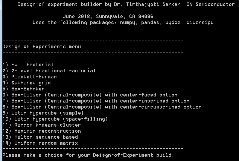
6 | of this software and associated documentation files (the "Software"), to deal
7 | in the Software without restriction, including without limitation the rights
8 | to use, copy, modify, merge, publish, distribute, sublicense, and/or sell
9 | copies of the Software, and to permit persons to whom the Software is
10 | furnished to do so, subject to the following conditions:
11 |
12 | The above copyright notice and this permission notice shall be included in all
13 | copies or substantial portions of the Software.
14 |
15 | THE SOFTWARE IS PROVIDED "AS IS", WITHOUT WARRANTY OF ANY KIND, EXPRESS OR
16 | IMPLIED, INCLUDING BUT NOT LIMITED TO THE WARRANTIES OF MERCHANTABILITY,
17 | FITNESS FOR A PARTICULAR PURPOSE AND NONINFRINGEMENT. IN NO EVENT SHALL THE
18 | AUTHORS OR COPYRIGHT HOLDERS BE LIABLE FOR ANY CLAIM, DAMAGES OR OTHER
19 | LIABILITY, WHETHER IN AN ACTION OF CONTRACT, TORT OR OTHERWISE, ARISING FROM,
20 | OUT OF OR IN CONNECTION WITH THE SOFTWARE OR THE USE OR OTHER DEALINGS IN THE
21 | SOFTWARE.
22 |
--------------------------------------------------------------------------------
/User_input.py:
--------------------------------------------------------------------------------
1 | # ===========================================================================================
2 | # Function for accepting the user input (choice) for desired DOE and the input CSV file name
3 | # ===========================================================================================
4 |
5 | def user_input():
6 | print("-"*60+"\n"+"Design of Experiments menu\n"+"-"*60+"\n")
7 | list_doe = ["1) Full factorial",
8 | "2) 2-level fractional factorial",
9 | "3) Plackett-Burman",
10 | "4) Sukharev grid",
11 | "5) Box-Behnken",
12 | "6) Box-Wilson (Central-composite) with center-faced option",
13 | "7) Box-Wilson (Central-composite) with center-inscribed option",
14 | "8) Box-Wilson (Central-composite) with center-circumscribed option",
15 | "9) Latin hypercube (simple)",
16 | "10) Latin hypercube (space-filling)",
17 | "11) Random k-means cluster",
18 | "12) Maximin reconstruction",
19 | "13) Halton sequence based",
20 | "14) Uniform random matrix"
21 | ]
22 |
23 | for choice in list_doe:
24 | print(choice)
25 | print("-"*60)
26 |
27 | doe_choice = int(input("Please make a choice for your Deisgn-of-Experiment build: "))
28 | infile = str(input("Please enter the name of the input csv file (enter only the name without the CSV extension): "))
29 | print()
30 |
31 | if (infile[-3:]!='csv'):
32 | infile=infile+'.csv'
33 |
34 | return (doe_choice,infile)
--------------------------------------------------------------------------------
/Read_Write_CSV.py:
--------------------------------------------------------------------------------
1 | import csv
2 |
3 | # ==========================================================
4 | # Function for reading a CSV file into a dictionary format
5 | # ==========================================================
6 |
7 | def read_variables_csv(csvfile):
8 | """
9 | Builds a Python dictionary object from an input CSV file.
10 | Helper function to read a CSV file on the disk, where user stores the limits/ranges of the process variables.
11 | """
12 | dict_key={}
13 | try:
14 | with open(csvfile) as f:
15 | reader = csv.DictReader(f)
16 | fields = reader.fieldnames
17 | for field in fields:
18 | lst=[]
19 | with open(csvfile) as f:
20 | reader = csv.DictReader(f)
21 | for row in reader:
22 | lst.append(float(row[field]))
23 | dict_key[field]=lst
24 |
25 | return dict_key
26 | except:
27 | print("Error in reading the specified file from the disk. Please make sure it is in current directory.")
28 | return -1
29 |
30 | # ===============================================================
31 | # Function for writing the design matrix into an output CSV file
32 | # ===============================================================
33 |
34 | def write_csv(df,filename):
35 | """
36 | Writes a CSV file on to the disk from the internal Pandas DataFrame object i.e. the computed design matrix
37 | """
38 | try:
39 | filename=filename+'.csv'
40 | df.to_csv(filename)
41 | except:
42 | return -1
--------------------------------------------------------------------------------
/.gitignore:
--------------------------------------------------------------------------------
1 | # Byte-compiled / optimized / DLL files
2 | __pycache__/
3 | *.py[cod]
4 | *$py.class
5 |
6 | # C extensions
7 | *.so
8 |
9 | # Distribution / packaging
10 | .Python
11 | build/
12 | develop-eggs/
13 | dist/
14 | downloads/
15 | eggs/
16 | .eggs/
17 | lib/
18 | lib64/
19 | parts/
20 | sdist/
21 | var/
22 | wheels/
23 | *.egg-info/
24 | .installed.cfg
25 | *.egg
26 | MANIFEST
27 |
28 | # PyInstaller
29 | # Usually these files are written by a python script from a template
30 | # before PyInstaller builds the exe, so as to inject date/other infos into it.
31 | *.manifest
32 | *.spec
33 |
34 | # Installer logs
35 | pip-log.txt
36 | pip-delete-this-directory.txt
37 |
38 | # Unit test / coverage reports
39 | htmlcov/
40 | .tox/
41 | .coverage
42 | .coverage.*
43 | .cache
44 | nosetests.xml
45 | coverage.xml
46 | *.cover
47 | .hypothesis/
48 | .pytest_cache/
49 |
50 | # Translations
51 | *.mo
52 | *.pot
53 |
54 | # Django stuff:
55 | *.log
56 | local_settings.py
57 | db.sqlite3
58 |
59 | # Flask stuff:
60 | instance/
61 | .webassets-cache
62 |
63 | # Scrapy stuff:
64 | .scrapy
65 |
66 | # Sphinx documentation
67 | docs/_build/
68 |
69 | # PyBuilder
70 | target/
71 |
72 | # Jupyter Notebook
73 | .ipynb_checkpoints
74 |
75 | # pyenv
76 | .python-version
77 |
78 | # celery beat schedule file
79 | celerybeat-schedule
80 |
81 | # SageMath parsed files
82 | *.sage.py
83 |
84 | # Environments
85 | .env
86 | .venv
87 | env/
88 | venv/
89 | ENV/
90 | env.bak/
91 | venv.bak/
92 |
93 | # Spyder project settings
94 | .spyderproject
95 | .spyproject
96 |
97 | # Rope project settings
98 | .ropeproject
99 |
100 | # mkdocs documentation
101 | /site
102 |
103 | # mypy
104 | .mypy_cache/
105 |
--------------------------------------------------------------------------------
/Main.py:
--------------------------------------------------------------------------------
1 | from Read_Write_CSV import *
2 | from Generate_DOE import *
3 | from User_input import *
4 |
5 | import time
6 |
7 | # ========================
8 | # Main execution function
9 | # ========================
10 |
11 | def execute_main():
12 | """
13 | Main function to execute the program.
14 | Calls "user_input" function to receive the choice of the DOE user wants to build and to read the input CSV file with the ranges of the variables. Thereafter, it calls the "generate_DOE" function to generate the DOE matrix and a suitable filename corresponding to the user's DOE choice. Finally, it calls the "write_CSV" function to write the DOE matrix (a Pandas DataFrame object) into a CSV file on the disk, and prints a message indicating the filename.
15 | """
16 | doe_choice, infile = user_input()
17 | df, filename = generate_DOE(doe_choice,infile)
18 | if type(df)!=int or type(filename)!=int:
19 | flag=write_csv(df,filename)
20 | if flag!=-1:
21 | print("\nAnalyzing input and building the DOE...",end=' ')
22 | time.sleep(2)
23 | print("DONE!!")
24 | time.sleep(0.5)
25 | print(f"Output has been written to the file: {filename}.csv")
26 | else:
27 | print("\nError in writing the output. \nIf you have a file open with same filename, please close it before running the command again!")
28 |
29 |
30 | #=====================================================
31 | # Main UX with simple information about the software
32 | #=====================================================
33 |
34 | print()
35 | print(" "*5+"Design-of-experiment builder by Dr. Tirthajyoti Sarkar, ON Semiconductor"+" "*5)
36 | print(" "*20+"June 2018, Sunnyvale, CA 94086"+" "*20)
37 | print(" "*10+"Uses the following packages: numpy, pandas, pydoe, diversipy"+" "*10)
38 | print()
39 |
40 | # Executes the main function
41 | execute_main()
--------------------------------------------------------------------------------
/doe_box_behnken.py:
--------------------------------------------------------------------------------
1 | """
2 | This code was originally published by the following individuals for use with
3 | Scilab:
4 | Copyright (C) 2012 - 2013 - Michael Baudin
5 | Copyright (C) 2012 - Maria Christopoulou
6 | Copyright (C) 2010 - 2011 - INRIA - Michael Baudin
7 | Copyright (C) 2009 - Yann Collette
8 | Copyright (C) 2009 - CEA - Jean-Marc Martinez
9 |
10 | website: forge.scilab.org/index.php/p/scidoe/sourcetree/master/macros
11 |
12 | Much thanks goes to these individuals. It has been converted to Python by
13 | Abraham Lee.
14 | """
15 |
16 | import numpy as np
17 | from pyDOE.doe_factorial import ff2n
18 | from pyDOE.doe_repeat_center import repeat_center
19 |
20 | __all__ = ['bbdesign']
21 |
22 | def bbdesign(n, center=None):
23 | """
24 | Create a Box-Behnken design
25 |
26 | Parameters
27 | ----------
28 | n : int
29 | The number of factors in the design
30 |
31 | Optional
32 | --------
33 | center : int
34 | The number of center points to include (default = 1).
35 |
36 | Returns
37 | -------
38 | mat : 2d-array
39 | The design matrix
40 |
41 | Example
42 | -------
43 | ::
44 |
45 | >>> bbdesign(3)
46 | array([[-1., -1., 0.],
47 | [ 1., -1., 0.],
48 | [-1., 1., 0.],
49 | [ 1., 1., 0.],
50 | [-1., 0., -1.],
51 | [ 1., 0., -1.],
52 | [-1., 0., 1.],
53 | [ 1., 0., 1.],
54 | [ 0., -1., -1.],
55 | [ 0., 1., -1.],
56 | [ 0., -1., 1.],
57 | [ 0., 1., 1.],
58 | [ 0., 0., 0.],
59 | [ 0., 0., 0.],
60 | [ 0., 0., 0.]])
61 |
62 | """
63 | assert n>=3, 'Number of variables must be at least 3'
64 |
65 | # First, compute a factorial DOE with 2 parameters
66 | H_fact = ff2n(2)
67 | # Now we populate the real DOE with this DOE
68 |
69 | # We made a factorial design on each pair of dimensions
70 | # - So, we created a factorial design with two factors
71 | # - Make two loops
72 | Index = 0
73 | nb_lines = int((0.5*n*(n-1))*H_fact.shape[0])
74 | H = repeat_center(n, nb_lines)
75 |
76 | for i in range(n - 1):
77 | for j in range(i + 1, n):
78 | Index = Index + 1
79 | H[max([0, (Index - 1)*H_fact.shape[0]]):Index*H_fact.shape[0], i] = H_fact[:, 0]
80 | H[max([0, (Index - 1)*H_fact.shape[0]]):Index*H_fact.shape[0], j] = H_fact[:, 1]
81 |
82 | if center is None:
83 | if n<=16:
84 | points= [0, 0, 0, 3, 3, 6, 6, 6, 8, 9, 10, 12, 12, 13, 14, 15, 16]
85 | center = points[n]
86 | else:
87 | center = n
88 |
89 | H = np.c_[H.T, repeat_center(n, center).T].T
90 |
91 | return H
92 |
--------------------------------------------------------------------------------
/Generate_DOE.py:
--------------------------------------------------------------------------------
1 | from DOE_functions import *
2 | from Read_Write_CSV import *
3 |
4 | # ====================================================================
5 | # Function to generate the DOE based on user's choice and input file
6 | # ====================================================================
7 |
8 | def generate_DOE(doe_choice, infile):
9 | """
10 | Generates the output design-of-experiment matrix by calling the appropriate function from the "DOE_function.py file".
11 | Returns the generated DataFrame (Pandas) and a filename (string) corresponding to the type of the DOE sought by the user. This filename string is used by the CSV writer function to write to the disk i.e. save the generated DataFrame in a CSV format.
12 | """
13 |
14 | dict_vars = read_variables_csv(infile)
15 | if type(dict_vars)!=int:
16 | factor_count=len(dict_vars)
17 | else:
18 | return (-1,-1)
19 |
20 | if doe_choice==1:
21 | df=build_full_fact(dict_vars)
22 | filename='Full_factorial_design'
23 |
24 | elif doe_choice==2:
25 | print("For this choice, you will be asked to enter a generator string expression. Please only use small letters e.g. 'a b c bc' for the string. Make sure to put a space in between every variable. Please note that the number of character blocks must be identical to the number of factors you have in your input file.\n")
26 | gen_string=str(input("Please enter the generator string for the fractional factorial build: "))
27 | print()
28 | if len(gen_string.split(' '))!=factor_count:
29 | print("Length of the generator string does not match the number of factors/variables. Sorry!")
30 | return (-1,-1)
31 | df=build_frac_fact(dict_vars,gen_string)
32 | filename='Fractional_factorial_design'
33 |
34 | elif doe_choice==3:
35 | df=build_plackett_burman(dict_vars)
36 | filename='Plackett_Burman_design'
37 |
38 | elif doe_choice==4:
39 | num_samples=int(input("Please enter the number of samples: "))
40 | print()
41 | df=build_sukharev(dict_vars,num_samples)
42 | filename='Sukharev_grid_design'
43 |
44 | elif doe_choice==5:
45 | num_center=int(input("Please enter the number of center points to be repeated (if more than one): "))
46 | print()
47 | df=build_box_behnken(dict_vars,num_center)
48 | filename='Box_Behnken_design'
49 |
50 | elif doe_choice==6:
51 | #num_center=int(input("Please enter the number of center points to be repeated (if more than one): "))
52 | print()
53 | df=build_central_composite(dict_vars,face='ccf')
54 | filename='Box_Wilson_face_centered_design'
55 |
56 | elif doe_choice==7:
57 | #num_center=int(input("Please enter the number of center points to be repeated (if more than one): "))
58 | print()
59 | df=build_central_composite(dict_vars,face='cci')
60 | filename='Box_Wilson_face_inscribed_design'
61 |
62 | elif doe_choice==8:
63 | #num_center=int(input("Please enter the number of center points to be repeated (if more than one): "))
64 | print()
65 | df=build_central_composite(dict_vars,face='ccc')
66 | filename='Box_Wilson_face_circumscribed_design'
67 |
68 | elif doe_choice==9:
69 | num_samples=int(input("Please enter the number of random sample points to generate: "))
70 | print()
71 | df=build_lhs(dict_vars,num_samples=num_samples)
72 | filename='Simple_Latin_Hypercube_design'
73 |
74 | elif doe_choice==10:
75 | num_samples=int(input("Please enter the number of random sample points to generate: "))
76 | print()
77 | df=build_space_filling_lhs(dict_vars,num_samples=num_samples)
78 | filename='Space_filling_Latin_Hypercube_design'
79 |
80 | elif doe_choice==11:
81 | num_samples=int(input("Please enter the number of random sample points to generate: "))
82 | print()
83 | df=build_random_k_means(dict_vars,num_samples=num_samples)
84 | filename='Random_k_means_design'
85 |
86 | elif doe_choice==12:
87 | num_samples=int(input("Please enter the number of random sample points to generate: "))
88 | print()
89 | df=build_maximin(dict_vars,num_samples=num_samples)
90 | filename='Maximin_reconstruction_design'
91 |
92 | elif doe_choice==13:
93 | num_samples=int(input("Please enter the number of random sample points to generate: "))
94 | print()
95 | df=build_halton(dict_vars,num_samples=num_samples)
96 | filename='Halton_sequence_design'
97 |
98 | elif doe_choice==14:
99 | num_samples=int(input("Please enter the number of random sample points to generate: "))
100 | print()
101 | df=build_uniform_random(dict_vars,num_samples=num_samples)
102 | filename='Uniform_random_matrix_design'
103 |
104 | return (df,filename)
--------------------------------------------------------------------------------
/doe_factorial.py:
--------------------------------------------------------------------------------
1 | """
2 | This code was originally published by the following individuals for use with
3 | Scilab:
4 | Copyright (C) 2012 - 2013 - Michael Baudin
5 | Copyright (C) 2012 - Maria Christopoulou
6 | Copyright (C) 2010 - 2011 - INRIA - Michael Baudin
7 | Copyright (C) 2009 - Yann Collette
8 | Copyright (C) 2009 - CEA - Jean-Marc Martinez
9 |
10 | website: forge.scilab.org/index.php/p/scidoe/sourcetree/master/macros
11 |
12 | Much thanks goes to these individuals. It has been converted to Python by
13 | Abraham Lee.
14 | """
15 |
16 | import re
17 | import numpy as np
18 |
19 | __all__ = ['np', 'fullfact', 'ff2n', 'fracfact']
20 |
21 | def fullfact(levels):
22 | """
23 | Create a general full-factorial design
24 |
25 | Parameters
26 | ----------
27 | levels : array-like
28 | An array of integers that indicate the number of levels of each input
29 | design factor.
30 |
31 | Returns
32 | -------
33 | mat : 2d-array
34 | The design matrix with coded levels 0 to k-1 for a k-level factor
35 |
36 | Example
37 | -------
38 | ::
39 |
40 | >>> fullfact([2, 4, 3])
41 | array([[ 0., 0., 0.],
42 | [ 1., 0., 0.],
43 | [ 0., 1., 0.],
44 | [ 1., 1., 0.],
45 | [ 0., 2., 0.],
46 | [ 1., 2., 0.],
47 | [ 0., 3., 0.],
48 | [ 1., 3., 0.],
49 | [ 0., 0., 1.],
50 | [ 1., 0., 1.],
51 | [ 0., 1., 1.],
52 | [ 1., 1., 1.],
53 | [ 0., 2., 1.],
54 | [ 1., 2., 1.],
55 | [ 0., 3., 1.],
56 | [ 1., 3., 1.],
57 | [ 0., 0., 2.],
58 | [ 1., 0., 2.],
59 | [ 0., 1., 2.],
60 | [ 1., 1., 2.],
61 | [ 0., 2., 2.],
62 | [ 1., 2., 2.],
63 | [ 0., 3., 2.],
64 | [ 1., 3., 2.]])
65 |
66 | """
67 | n = len(levels) # number of factors
68 | nb_lines = np.prod(levels) # number of trial conditions
69 | H = np.zeros((nb_lines, n))
70 |
71 | level_repeat = 1
72 | range_repeat = np.prod(levels)
73 | for i in range(n):
74 | range_repeat //= levels[i]
75 | lvl = []
76 | for j in range(levels[i]):
77 | lvl += [j]*level_repeat
78 | rng = lvl*range_repeat
79 | level_repeat *= levels[i]
80 | H[:, i] = rng
81 |
82 | return H
83 |
84 | ################################################################################
85 |
86 | def ff2n(n):
87 | """
88 | Create a 2-Level full-factorial design
89 |
90 | Parameters
91 | ----------
92 | n : int
93 | The number of factors in the design.
94 |
95 | Returns
96 | -------
97 | mat : 2d-array
98 | The design matrix with coded levels -1 and 1
99 |
100 | Example
101 | -------
102 | ::
103 |
104 | >>> ff2n(3)
105 | array([[-1., -1., -1.],
106 | [ 1., -1., -1.],
107 | [-1., 1., -1.],
108 | [ 1., 1., -1.],
109 | [-1., -1., 1.],
110 | [ 1., -1., 1.],
111 | [-1., 1., 1.],
112 | [ 1., 1., 1.]])
113 |
114 | """
115 | return 2*fullfact([2]*n) - 1
116 |
117 | ################################################################################
118 |
119 | def fracfact(gen):
120 | """
121 | Create a 2-level fractional-factorial design with a generator string.
122 |
123 | Parameters
124 | ----------
125 | gen : str
126 | A string, consisting of lowercase, uppercase letters or operators "-"
127 | and "+", indicating the factors of the experiment
128 |
129 | Returns
130 | -------
131 | H : 2d-array
132 | A m-by-n matrix, the fractional factorial design. m is 2^k, where k
133 | is the number of letters in ``gen``, and n is the total number of
134 | entries in ``gen``.
135 |
136 | Notes
137 | -----
138 | In ``gen`` we define the main factors of the experiment and the factors
139 | whose levels are the products of the main factors. For example, if
140 |
141 | gen = "a b ab"
142 |
143 | then "a" and "b" are the main factors, while the 3rd factor is the product
144 | of the first two. If we input uppercase letters in ``gen``, we get the same
145 | result. We can also use the operators "+" and "-" in ``gen``.
146 |
147 | For example, if
148 |
149 | gen = "a b -ab"
150 |
151 | then the 3rd factor is the opposite of the product of "a" and "b".
152 |
153 | The output matrix includes the two level full factorial design, built by
154 | the main factors of ``gen``, and the products of the main factors. The
155 | columns of ``H`` follow the sequence of ``gen``.
156 |
157 | For example, if
158 |
159 | gen = "a b ab c"
160 |
161 | then columns H[:, 0], H[:, 1], and H[:, 3] include the two level full
162 | factorial design and H[:, 2] includes the products of the main factors.
163 |
164 | Examples
165 | --------
166 | ::
167 |
168 | >>> fracfact("a b ab")
169 | array([[-1., -1., 1.],
170 | [ 1., -1., -1.],
171 | [-1., 1., -1.],
172 | [ 1., 1., 1.]])
173 |
174 | >>> fracfact("A B AB")
175 | array([[-1., -1., 1.],
176 | [ 1., -1., -1.],
177 | [-1., 1., -1.],
178 | [ 1., 1., 1.]])
179 |
180 | >>> fracfact("a b -ab c +abc")
181 | array([[-1., -1., -1., -1., -1.],
182 | [ 1., -1., 1., -1., 1.],
183 | [-1., 1., 1., -1., 1.],
184 | [ 1., 1., -1., -1., -1.],
185 | [-1., -1., -1., 1., 1.],
186 | [ 1., -1., 1., 1., -1.],
187 | [-1., 1., 1., 1., -1.],
188 | [ 1., 1., -1., 1., 1.]])
189 |
190 | """
191 | # Recognize letters and combinations
192 | A = [item for item in re.split('\-?\s?\+?', gen) if item] # remove empty strings
193 | C = [len(item) for item in A]
194 |
195 | # Indices of single letters (main factors)
196 | I = [i for i, item in enumerate(C) if item==1]
197 |
198 | # Indices of letter combinations (we need them to fill out H2 properly).
199 | J = [i for i, item in enumerate(C) if item!=1]
200 |
201 | # Check if there are "-" or "+" operators in gen
202 | U = [item for item in gen.split(' ') if item] # remove empty strings
203 |
204 | # If R1 is either None or not, the result is not changed, since it is a
205 | # multiplication of 1.
206 | R1 = _grep(U, '+')
207 | R2 = _grep(U, '-')
208 |
209 | # Fill in design with two level factorial design
210 | H1 = ff2n(len(I))
211 | H = np.zeros((H1.shape[0], len(C)))
212 | H[:, I] = H1
213 |
214 | # Recognize combinations and fill in the rest of matrix H2 with the proper
215 | # products
216 | for k in J:
217 | # For lowercase letters
218 | xx = np.array([ord(c) for c in A[k]]) - 97
219 |
220 | # For uppercase letters
221 | if np.any(xx<0):
222 | xx = np.array([ord(c) for c in A[k]]) - 65
223 |
224 | H[:, k] = np.prod(H1[:, xx], axis=1)
225 |
226 | # Update design if gen includes "-" operator
227 | if R2:
228 | H[:, R2] *= -1
229 |
230 | # Return the fractional factorial design
231 | return H
232 |
233 | def _grep(haystack, needle):
234 | try:
235 | haystack[0]
236 | except (TypeError, AttributeError):
237 | return [0] if needle in haystack else []
238 | else:
239 | locs = []
240 | for idx, item in enumerate(haystack):
241 | if needle in item:
242 | locs += [idx]
243 | return locs
244 |
--------------------------------------------------------------------------------
/pyDOE_corrected.py:
--------------------------------------------------------------------------------
1 | """
2 | This code was originally published by the following individuals for use with
3 | Scilab:
4 | Copyright (C) 2012 - 2013 - Michael Baudin
5 | Copyright (C) 2012 - Maria Christopoulou
6 | Copyright (C) 2010 - 2011 - INRIA - Michael Baudin
7 | Copyright (C) 2009 - Yann Collette
8 | Copyright (C) 2009 - CEA - Jean-Marc Martinez
9 |
10 | website: forge.scilab.org/index.php/p/scidoe/sourcetree/master/macros
11 |
12 | Much thanks goes to these individuals. It has been converted to Python by
13 | Abraham Lee.
14 | """
15 |
16 | import re
17 | import numpy as np
18 |
19 | #__all__ = ['np', 'fullfact_corrected', 'ff2n', 'fracfact']
20 |
21 | def fullfact_corrected(levels):
22 | """
23 | Create a general full-factorial design
24 |
25 | Parameters
26 | ----------
27 | levels : array-like
28 | An array of integers that indicate the number of levels of each input
29 | design factor.
30 |
31 | Returns
32 | -------
33 | mat : 2d-array
34 | The design matrix with coded levels 0 to k-1 for a k-level factor
35 |
36 | Example
37 | -------
38 | ::
39 |
40 | >>> fullfact([2, 4, 3])
41 | array([[ 0., 0., 0.],
42 | [ 1., 0., 0.],
43 | [ 0., 1., 0.],
44 | [ 1., 1., 0.],
45 | [ 0., 2., 0.],
46 | [ 1., 2., 0.],
47 | [ 0., 3., 0.],
48 | [ 1., 3., 0.],
49 | [ 0., 0., 1.],
50 | [ 1., 0., 1.],
51 | [ 0., 1., 1.],
52 | [ 1., 1., 1.],
53 | [ 0., 2., 1.],
54 | [ 1., 2., 1.],
55 | [ 0., 3., 1.],
56 | [ 1., 3., 1.],
57 | [ 0., 0., 2.],
58 | [ 1., 0., 2.],
59 | [ 0., 1., 2.],
60 | [ 1., 1., 2.],
61 | [ 0., 2., 2.],
62 | [ 1., 2., 2.],
63 | [ 0., 3., 2.],
64 | [ 1., 3., 2.]])
65 |
66 | """
67 | n = len(levels) # number of factors
68 | nb_lines = np.prod(levels) # number of trial conditions
69 | H = np.zeros((nb_lines, n))
70 |
71 | level_repeat = 1
72 | range_repeat = np.prod(levels)
73 | for i in range(n):
74 | range_repeat //= levels[i]
75 | lvl = []
76 | for j in range(levels[i]):
77 | lvl += [j]*level_repeat
78 | rng = lvl*range_repeat
79 | level_repeat *= levels[i]
80 | H[:, i] = rng
81 |
82 | return H
83 |
84 | ################################################################################
85 |
86 | def ff2n(n):
87 | """
88 | Create a 2-Level full-factorial design
89 |
90 | Parameters
91 | ----------
92 | n : int
93 | The number of factors in the design.
94 |
95 | Returns
96 | -------
97 | mat : 2d-array
98 | The design matrix with coded levels -1 and 1
99 |
100 | Example
101 | -------
102 | ::
103 |
104 | >>> ff2n(3)
105 | array([[-1., -1., -1.],
106 | [ 1., -1., -1.],
107 | [-1., 1., -1.],
108 | [ 1., 1., -1.],
109 | [-1., -1., 1.],
110 | [ 1., -1., 1.],
111 | [-1., 1., 1.],
112 | [ 1., 1., 1.]])
113 |
114 | """
115 | return 2*fullfact_corrected([2]*n) - 1
116 |
117 | ################################################################################
118 |
119 | def fracfact(gen):
120 | """
121 | Create a 2-level fractional-factorial design with a generator string.
122 |
123 | Parameters
124 | ----------
125 | gen : str
126 | A string, consisting of lowercase, uppercase letters or operators "-"
127 | and "+", indicating the factors of the experiment
128 |
129 | Returns
130 | -------
131 | H : 2d-array
132 | A m-by-n matrix, the fractional factorial design. m is 2^k, where k
133 | is the number of letters in ``gen``, and n is the total number of
134 | entries in ``gen``.
135 |
136 | Notes
137 | -----
138 | In ``gen`` we define the main factors of the experiment and the factors
139 | whose levels are the products of the main factors. For example, if
140 |
141 | gen = "a b ab"
142 |
143 | then "a" and "b" are the main factors, while the 3rd factor is the product
144 | of the first two. If we input uppercase letters in ``gen``, we get the same
145 | result. We can also use the operators "+" and "-" in ``gen``.
146 |
147 | For example, if
148 |
149 | gen = "a b -ab"
150 |
151 | then the 3rd factor is the opposite of the product of "a" and "b".
152 |
153 | The output matrix includes the two level full factorial design, built by
154 | the main factors of ``gen``, and the products of the main factors. The
155 | columns of ``H`` follow the sequence of ``gen``.
156 |
157 | For example, if
158 |
159 | gen = "a b ab c"
160 |
161 | then columns H[:, 0], H[:, 1], and H[:, 3] include the two level full
162 | factorial design and H[:, 2] includes the products of the main factors.
163 |
164 | Examples
165 | --------
166 | ::
167 |
168 | >>> fracfact("a b ab")
169 | array([[-1., -1., 1.],
170 | [ 1., -1., -1.],
171 | [-1., 1., -1.],
172 | [ 1., 1., 1.]])
173 |
174 | >>> fracfact("A B AB")
175 | array([[-1., -1., 1.],
176 | [ 1., -1., -1.],
177 | [-1., 1., -1.],
178 | [ 1., 1., 1.]])
179 |
180 | >>> fracfact("a b -ab c +abc")
181 | array([[-1., -1., -1., -1., -1.],
182 | [ 1., -1., 1., -1., 1.],
183 | [-1., 1., 1., -1., 1.],
184 | [ 1., 1., -1., -1., -1.],
185 | [-1., -1., -1., 1., 1.],
186 | [ 1., -1., 1., 1., -1.],
187 | [-1., 1., 1., 1., -1.],
188 | [ 1., 1., -1., 1., 1.]])
189 |
190 | """
191 | # Recognize letters and combinations
192 | A = [item for item in re.split('\-?\s?\+?', gen) if item] # remove empty strings
193 | C = [len(item) for item in A]
194 |
195 | # Indices of single letters (main factors)
196 | I = [i for i, item in enumerate(C) if item==1]
197 |
198 | # Indices of letter combinations (we need them to fill out H2 properly).
199 | J = [i for i, item in enumerate(C) if item!=1]
200 |
201 | # Check if there are "-" or "+" operators in gen
202 | U = [item for item in gen.split(' ') if item] # remove empty strings
203 |
204 | # If R1 is either None or not, the result is not changed, since it is a
205 | # multiplication of 1.
206 | R1 = _grep(U, '+')
207 | R2 = _grep(U, '-')
208 |
209 | # Fill in design with two level factorial design
210 | H1 = ff2n(len(I))
211 | H = np.zeros((H1.shape[0], len(C)))
212 | H[:, I] = H1
213 |
214 | # Recognize combinations and fill in the rest of matrix H2 with the proper
215 | # products
216 | for k in J:
217 | # For lowercase letters
218 | xx = np.array([ord(c) for c in A[k]]) - 97
219 |
220 | # For uppercase letters
221 | if np.any(xx<0):
222 | xx = np.array([ord(c) for c in A[k]]) - 65
223 |
224 | H[:, k] = np.prod(H1[:, xx], axis=1)
225 |
226 | # Update design if gen includes "-" operator
227 | if R2:
228 | H[:, R2] *= -1
229 |
230 | # Return the fractional factorial design
231 | return H
232 |
233 | def _grep(haystack, needle):
234 | try:
235 | haystack[0]
236 | except (TypeError, AttributeError):
237 | return [0] if needle in haystack else []
238 | else:
239 | locs = []
240 | for idx, item in enumerate(haystack):
241 | if needle in item:
242 | locs += [idx]
243 | return locs
244 |
245 |
246 | #__all__ = ['bbdesign_corrected']
247 |
248 | def bbdesign_corrected(n, center=None):
249 | """
250 | Create a Box-Behnken design
251 |
252 | Parameters
253 | ----------
254 | n : int
255 | The number of factors in the design
256 |
257 | Optional
258 | --------
259 | center : int
260 | The number of center points to include (default = 1).
261 |
262 | Returns
263 | -------
264 | mat : 2d-array
265 | The design matrix
266 |
267 | Example
268 | -------
269 | ::
270 |
271 | >>> bbdesign(3)
272 | array([[-1., -1., 0.],
273 | [ 1., -1., 0.],
274 | [-1., 1., 0.],
275 | [ 1., 1., 0.],
276 | [-1., 0., -1.],
277 | [ 1., 0., -1.],
278 | [-1., 0., 1.],
279 | [ 1., 0., 1.],
280 | [ 0., -1., -1.],
281 | [ 0., 1., -1.],
282 | [ 0., -1., 1.],
283 | [ 0., 1., 1.],
284 | [ 0., 0., 0.],
285 | [ 0., 0., 0.],
286 | [ 0., 0., 0.]])
287 |
288 | """
289 | assert n>=3, 'Number of variables must be at least 3'
290 |
291 | # First, compute a factorial DOE with 2 parameters
292 | H_fact = ff2n(2)
293 | # Now we populate the real DOE with this DOE
294 |
295 | # We made a factorial design on each pair of dimensions
296 | # - So, we created a factorial design with two factors
297 | # - Make two loops
298 | Index = 0
299 | nb_lines = int((0.5*n*(n-1))*H_fact.shape[0])
300 | H = repeat_center(n, nb_lines)
301 |
302 | for i in range(n - 1):
303 | for j in range(i + 1, n):
304 | Index = Index + 1
305 | H[max([0, (Index - 1)*H_fact.shape[0]]):Index*H_fact.shape[0], i] = H_fact[:, 0]
306 | H[max([0, (Index - 1)*H_fact.shape[0]]):Index*H_fact.shape[0], j] = H_fact[:, 1]
307 |
308 | if center is None:
309 | if n<=16:
310 | points= [0, 0, 0, 3, 3, 6, 6, 6, 8, 9, 10, 12, 12, 13, 14, 15, 16]
311 | center = points[n]
312 | else:
313 | center = n
314 |
315 | H = np.c_[H.T, repeat_center(n, center).T].T
316 |
317 | return H
318 |
319 | def repeat_center(n, repeat):
320 | """
321 | Create the center-point portion of a design matrix
322 |
323 | Parameters
324 | ----------
325 | n : int
326 | The number of factors in the original design
327 | repeat : int
328 | The number of center points to repeat
329 |
330 | Returns
331 | -------
332 | mat : 2d-array
333 | The center-point portion of a design matrix (elements all zero).
334 |
335 | Example
336 | -------
337 | ::
338 |
339 | >>> repeat_center(3, 2)
340 | array([[ 0., 0., 0.],
341 | [ 0., 0., 0.]])
342 |
343 | """
344 | return np.zeros((repeat, n))
345 |
--------------------------------------------------------------------------------
/README.md:
--------------------------------------------------------------------------------
1 | # Design-of-experiment (DOE) matrix generator for engineering and statistics
2 |
3 |
4 | ### Copyright Notice and Code repository
5 | ***Copyright (c): 2018-2028, Dr. Tirthajyoti Sarkar, Sunnyvale, CA 94086***
6 |
7 | It uses a MIT License, so although I retain the copyright of this particular code, please feel free to exercise your rights of the free software by using and enhancing it.
8 |
9 | Please get the codebase from [here](https://github.com/tirthajyoti/Design-of-experiment-Python).
10 |
11 | ## UPDATE (July 2019)
12 |
13 | A formal PyPi-hosted package `doepy` has been released (Alpha 0.0.1 version). [Here is the Github repo](https://github.com/tirthajyoti/doepy).
14 |
15 | You can easy install the package by **`pip install doepy`** and use that for generating CSV files of design tables.
16 |
17 | All the design schemes, mentioned in this repo, are supported in this package now.
18 |
19 | [READ the Docs here](https://doepy.readthedocs.io/en/latest/).
20 |
21 | ## Table of Contents
22 | 1. [Introduction](#Introduction)
23 | * [What is a scientific experiment?](#ScienceExp)
24 | * [What is Experimental Design?](#ExpDesign)
25 | * [Options for open-source DOE builder package in Python?](#PythonOpenSource)
26 | 2. [Features](#Features)
27 | * [Limitation of the foundation packages used](#Limitations)
28 | * [Simplified user interface](#SimpleUI)
29 | * [Designs available](#DesignOptions)
30 | 3. [How to use it?](#HowTo)
31 | * [What supporitng packages are required?](#SupportingPackages)
32 | * [Eratta for using PyDOE](#Eratta)
33 | * [How to run the program?](#HowToRun)
34 | * [Is an installer/Python library available?](#Installer)
35 | 4. [Examples](#Examples)
36 | * [Full-factorial design](#FullFactorial)
37 | * [Fractional-factorial design](#FracFactorial)
38 | * [Central-composite design](#CentralComposite)
39 | * [Latin Hypercube design](#LatinHypercube)
40 | 5. [Acknowledgements and Requirements](#Acknowledgement)
41 |
42 | ## Introduction
43 | [Design of Experiment (DOE)](https://en.wikipedia.org/wiki/Design_of_experiments) is an important activity for any scientist, engineer, or statistician planning to conduct experimental analysis. This exercise has become **critical in this age of rapidly expanding field of data science and associated statistical modeling and machine learning**. A well-planned DOE can give a researcher meaningful data set to act upon with optimal number of experiments preserving critical resources.
44 |
45 | > After all, aim of Data Science is essentially to conduct highest quality scientific investigation and modeling with real world data. And to do good science with data, one needs to collect it through carefully thought-out experiment to cover all corner cases and reduce any possible bias.
46 |
47 | ### What is a scientific experiment?
48 | In its simplest form, a scientific experiment aims at predicting the outcome by introducing a change of the preconditions, which is represented by one or more [independent variables](https://en.wikipedia.org/wiki/Dependent_and_independent_variables), also referred to as “input variables” or “predictor variables.” The change in one or more independent variables is generally hypothesized to result in a change in one or more [dependent variables](https://en.wikipedia.org/wiki/Dependent_and_independent_variables), also referred to as “output variables” or “response variables.” The experimental design may also identify [control variables](https://en.wikipedia.org/wiki/Controlling_for_a_variable) that must be held constant to prevent external factors from affecting the results.
49 |
50 | ### What is Experimental Design?
51 | Experimental design involves not only the selection of suitable independent, dependent, and control variables, but planning the delivery of the experiment under statistically optimal conditions given the constraints of available resources. There are multiple approaches for determining the set of design points (unique combinations of the settings of the independent variables) to be used in the experiment.
52 |
53 | Main concerns in experimental design include the establishment of [validity](https://en.wikipedia.org/wiki/Validity_%28statistics%29), [reliability](https://en.wikipedia.org/wiki/Reliability_%28statistics%29), and [replicability](https://en.wikipedia.org/wiki/Reproducibility). For example, these concerns can be partially addressed by carefully choosing the independent variable, reducing the risk of measurement error, and ensuring that the documentation of the method is sufficiently detailed. Related concerns include achieving appropriate levels of [statistical power](https://en.wikipedia.org/wiki/Statistical_power) and [sensitivity](https://en.wikipedia.org/wiki/Sensitivity_and_specificity).
54 |
55 | Need for careful design of experiment arises in all fields of serious scientific, technological, and even social science investigation — *computer science, physics, geology, political science, electrical engineering, psychology, business marketing analysis, financial analytics*, etc…
56 |
57 | ### Options for open-source DOE builder package in Python?
58 | Unfortunately, majority of the state-of-the-art DOE generators are part of commercial statistical software packages like [JMP (SAS)](https://www.jmp.com/) or [Minitab](www.minitab.com/en-US/default.aspx). However, a researcher will surely be benefited if there exists an open-source code which presents an intuitive user interface for generating an experimental design plan from a simple list of input variables. There are a couple of DOE builder Python packages but individually they don’t cover all the necessary DOE methods and they lack a simplified user API, where one can just input a CSV file of input variables’ range and get back the DOE matrix in another CSV file.
59 |
60 | ## Features
61 | This set of codes is a collection of functions which wrap around the core packages (mentioned below) and generate **design-of-experiment (DOE) matrices** for a statistician or engineer from an arbitrary range of input variables.
62 |
63 | ### Limitation of the foundation packages used
64 | Both the core packages, which act as foundations to this repo, are not complete in the sense that they do not cover all the necessary functions to generate DOE table that a design engineer may need while planning an experiment. Also, they offer only low-level APIs in the sense that the standard output from them are normalized numpy arrays. It was felt that users, who may not be comfortable in dealing with Python objects directly, should be able to take advantage of their functionalities through a simplified user interface.
65 |
66 | ### Simplified user interface
67 | ***User just needs to provide a simple CSV file with a single table of variables and their ranges (2-level i.e. min/max or 3-level).*** Some of the functions work with 2-level min/max range while some others need 3-level ranges from the user (low-mid-high). Intelligence is built into the code to handle the case if the range input is not appropriate and to generate levels by simple linear interpolation from the given input. The code will generate the DOE as per user's choice and write the matrix in a CSV file on to the disk. In this way, ***the only API user is exposed to are input and output CSV files. These files then can be used in any engineering simulator, software, process-control module, or fed into process equipments.***
68 |
69 | ### Designs available
70 | * Full factorial,
71 | * 2-level fractional factorial,
72 | * Plackett-Burman,
73 | * Sukharev grid,
74 | * Box-Behnken,
75 | * Box-Wilson (Central-composite) with center-faced option,
76 | * Box-Wilson (Central-composite) with center-inscribed option,
77 | * Box-Wilson (Central-composite) with center-circumscribed option,
78 | * Latin hypercube (simple),
79 | * Latin hypercube (space-filling),
80 | * Random k-means cluster,
81 | * Maximin reconstruction,
82 | * Halton sequence based,
83 | * Uniform random matrix
84 |
85 | ## How to use it?
86 | ### What supporitng packages are required?
87 | First make sure you have all the necessary packages installed. You can simply run the .bash (Unix/Linux) and .bat (Windows) files provided in the repo, to install those packages from your command line interface. They contain the following commands,
88 |
89 | ```
90 | pip install numpy
91 | pip install pandas
92 | pip install matplotlib
93 | pip install pydoe
94 | pip install diversipy
95 | ```
96 | ### Eratta for using PyDOE
97 | Please note that as installed, PyDOE will throw some error related to type conversion. There are two options
98 | * I have modified the pyDOE code suitably and included a file with re-written functions in the repo. This is the file called by the program while executing, so you should see no error.
99 | * If you encounter any error, you could try to modify the PyDOE code by going to the folder where pyDOE files are copied and copying the two files `doe_factorial.py` and `doe_box_behnken.py` supplied with this repo.
100 |
101 | ### How to run the program?
102 | Note this is just a code repository and not a installer package. For the time being, please clone [this repo from GitHub](https://github.com/tirthajyoti/Design-of-experiment-Python), store all the files in a local directory.
103 |
104 | **``git clone https://github.com/tirthajyoti/Design-of-experiment-Python.git``**
105 |
106 | Then start using the software by simply typing,
107 |
108 | **``python Main.py``**
109 |
110 | After this, a simple menu will be printed on the screen and you will be prompted for a choice of number (a DOE) and name of the input CSV file (containing the names and ranges of your variables).
111 |
112 |
113 |
114 | **You must have an input parameters CSV file stored in the same directory** that you are running this code from. You should use the supplied generic CSV file as an example. Please put the factors in the columns and the levels in the row (not the other way around). Couple of example CSV files are provided in the repo. Feel free to modify them as per your needs.
115 |
116 | ### Is an installer/Python library available?
117 | At this time, **No**. I plan to work on turning this into a full-fledged Python library which can be installed from PyPi repository by a PIP command. But I cannot promise any timeline for that :-) ***If somebody wants to collaborate and work on an installer, please feel free to do so.***
118 |
119 | ## Examples
120 | Let's say the input file contains the following table for the parameters range. Imagine this as a generic example of a checmical process in a plant.
121 |
122 | Pressure | Temperature | FlowRate | Time
123 | ------------ | ------------- | -------------|-----------------
124 | 40 | 290 | 0.2 | 5
125 | 55 | 320 | 0.3 | 8
126 | 70 | 350 | 0.4 | 11
127 |
128 | ### Full-factorial design
129 |
130 |
131 |
132 | If we build a full-factorial DOE out of this, we will get a table with 81 entries because 4 factors permuted in 3 levels result in 3^4=81 combinations!
133 |
134 | Pressure | Temperature | FlowRate | Time
135 | ------------ | ------------- | -------------|-----------------
136 | 40 | 290 | 0.2 | 5
137 | 50 | 290 | 0.2 | 5
138 | 70 | 290 | 0.2 | 5
139 | 40 | 320 | 0.2 | 5
140 | 50 | 320 | 0.2 | 5
141 | 70 | 320 | 0.2 | 5
142 | ... | ... | ... | ...
143 | ...| ... | ... | ...
144 | 40 | 290 | 0.3 | 8
145 | 50 | 290 | 0.3 | 8
146 | 70 | 290 | 0.3 | 8
147 | 40 | 320 | 0.3 | 8
148 | 50 | 320 | 0.3 | 8
149 | 70 | 320 | 0.3 | 8
150 | ... | ... | ... | ...
151 | ...| ... | ... | ...
152 | 40 | 320 | 0.4 | 11
153 | 50 | 320 | 0.4 | 11
154 | 70 | 320 | 0.4 | 11
155 | 40 | 350 | 0.4 | 11
156 | 50 | 350 | 0.4 | 11
157 | 70 | 350 | 0.4 | 11
158 |
159 | ### Fractional-factorial design
160 | Clearly the full-factorial designs grows quickly! Engineers and scientists therefore often use half-factorial/fractional-factorial designs where they confound one or more factors with other factors and build a reduced DOE. Let's say we decide to build a 2-level fractional factorial of this set of variables with the 4th variables as the confounding factor (i.e. not an independent variable but as a function of other variables). If the functional relationship is "A B C BC" i.e. the 4th parameter vary depending only on 2nd and 3rd parameter, the output table could look like,
161 |
162 | Pressure | Temperature | FlowRate | Time
163 | ------------ | ------------- | -------------|-----------------
164 | 40 | 290 | 0.2 | 11
165 | 70 | 290 | 0.2 | 11
166 | 40 | 350 | 0.2 | 5
167 | 70 | 350 | 0.2 | 5
168 | 40 | 290 | 0.4 | 5
169 | 70 | 290 | 0.4 | 5
170 | 40 | 350 | 0.4 | 11
171 | 70 | 350 | 0.4 | 11
172 |
173 | ### Central-composite design
174 |
175 | A Box-Wilson Central Composite Design, commonly called 'a central composite design,' contains an imbedded factorial or fractional factorial design with center points that is augmented with a group of 'star points' that allow estimation of curvature. One central composite design consists of cube points at the corners of a unit cube that is the product of the intervals [-1,1], star points along the axes at or outside the cube, and center points at the origin. Central composite designs are of three types. Circumscribed (CCC) designs are as described above. Inscribed (CCI) designs are as described above, but scaled so the star points take the values -1 and +1, and the cube points lie in the interior of the cube. Faced (CCF) designs have the star points on the faces of the cube. Faced designs have three levels per factor, in contrast with the other types that have five levels per factor. The following figure shows these three types of designs for three factors. [Read this page] (http://blog.minitab.com/blog/understanding-statistics/getting-started-with-factorial-design-of-experiments-doe) for more information about this kind of design philosophy.
176 |
177 | ### Latin Hypercube design
178 |
179 |
180 | Sometimes, a set of ***randomized design points within a given range*** could be attractive for the experimenter to asses the impact of the process variables on the output. [Monte Carlo simulations](https://en.wikipedia.org/wiki/Monte_Carlo_method) are close example of this approach. However, a Latin Hypercube design is better choice for experimental design rather than building a complete random matrix as it tries to subdivide the sample space in smaller cells and choose only one element out of each subcell. This way, a more ***'uniform spreading' of the random sample points*** can be obtained. User can choose the density of sample points. For example, if we choose to generate a Latin Hypercube of 12 experiments from the same input files, that could look like,
181 |
182 | Pressure | Temperature | FlowRate | Time
183 | ------------ | ------------- | -------------|-----------------
184 | 63.16 | 313.32 | 0.37 | 10.52
185 | 61.16 | 343.88 | 0.23 | 5.04
186 | 57.83 | 327.46 | 0.35 | 9.47
187 | 68.61 | 309.81 | 0.35 | 8.39
188 | 66.01 | 301.29 | 0.22 | 6.34
189 | 45.76 | 347.97 | 0.27 | 6.94
190 | 40.48 | 320.72 | 0.29 | 9.68
191 | 51.46 | 293.35 | 0.20 | 7.11
192 | 43.63 | 334.92 | 0.30 | 7.66
193 | 47.87 | 339.68 | 0.26 | 8.59
194 | 55.28 | 317.68 | 0.39 | 5.61
195 | 53.99 | 297.07 | 0.32 | 10.43
196 |
197 | Of course, there is no guarantee that you will get the same matrix if you run this function because this are randomly sampled, but you get the idea!
198 |
199 | ## Acknowledgements and Requirements
200 | The code was written in Python 3.6. It uses following external packages that needs to be installed on your system to use it,
201 | * pydoe: A package designed to help the scientist, engineer, statistician, etc., to construct appropriate experimental designs. [Check the docs here](https://pythonhosted.org/pyDOE/).
202 | * diversipy: A collection of algorithms for sampling in hypercubes, selecting diverse subsets, and measuring diversity. [Check the docs here](https://www.simonwessing.de/diversipy/doc/).
203 | * numpy
204 | * pandas
205 |
--------------------------------------------------------------------------------
/DOE_functions.py:
--------------------------------------------------------------------------------
1 | #====================
2 | # Essential imports
3 | #====================
4 | from pyDOE import *
5 | from pyDOE_corrected import *
6 | from diversipy import *
7 | import pandas as pd
8 | import numpy as np
9 |
10 | # ===========================================================================================================
11 | # Function for constructing a DataFrame from a numpy array generated by PyDOE function and individual lists
12 | # ===========================================================================================================
13 |
14 | def construct_df(x,r):
15 | df=pd.DataFrame(data=x,dtype='float32')
16 | for i in df.index:
17 | for j in range(len(list(df.iloc[i]))):
18 | df.iloc[i][j]=r[j][int(df.iloc[i][j])]
19 | return df
20 |
21 | # ===================================================================================================
22 | # Function for constructing a DataFrame from a matrix with floating point numbers between -1 and +1
23 | # ===================================================================================================
24 |
25 | def construct_df_from_matrix(x,factor_array):
26 | """
27 | This function constructs a DataFrame out of x and factor_array, both of which are assumed to be numpy arrays.
28 | It projects the numbers in the x (which is output of a design-of-experiment build) to the factor array ranges.
29 | Here factor_array is assumed to have only min and max ranges.
30 | Matrix x is assumed to have numbers ranging from -1 to 1.
31 | """
32 |
33 | row_num=x.shape[0] # Number of rows in the matrix x
34 | col_num=x.shape[1] # Number of columns in the matrix x
35 |
36 | empty=np.zeros((row_num,col_num))
37 |
38 | def simple_substitution(idx,factor_list):
39 | if idx==-1:
40 | return factor_list[0]
41 | elif idx==0:
42 | return factor_list[1]
43 | elif idx==1:
44 | return factor_list[2]
45 | else:
46 | alpha=np.abs(factor_list[2]-factor_list[0])/2
47 | if idx<0:
48 | beta=np.abs(idx)-1
49 | return factor_list[0]-(beta*alpha)
50 | else:
51 | beta=idx-1
52 | return factor_list[2]+(beta*alpha)
53 |
54 | for i in range(row_num):
55 | for j in range(col_num):
56 | empty[i,j] = simple_substitution(x[i,j],factor_array[j])
57 |
58 | return pd.DataFrame(data=empty)
59 |
60 | # =================================================================================================
61 | # Function for constructing a DataFrame from a matrix with floating point numbers between 0 and 1
62 | # =================================================================================================
63 |
64 | def construct_df_from_random_matrix(x,factor_array):
65 | """
66 | This function constructs a DataFrame out of matrix x and factor_array, both of which are assumed to be numpy arrays.
67 | It projects the numbers in the x (which is output of a design-of-experiment build) to the factor array ranges.
68 | Here factor_array is assumed to have only min and max ranges.
69 | Matrix x is assumed to have numbers ranging from 0 to 1 only.
70 | """
71 |
72 | row_num=x.shape[0] # Number of rows in the matrix x
73 | col_num=x.shape[1] # Number of columns in the matrix x
74 |
75 | empty=np.zeros((row_num,col_num))
76 |
77 | def simple_substitution(idx,factor_list):
78 | alpha=np.abs(factor_list[1]-factor_list[0])
79 | beta=idx
80 | return factor_list[0]+(beta*alpha)
81 |
82 | for i in range(row_num):
83 | for j in range(col_num):
84 | empty[i,j] = simple_substitution(x[i,j],factor_array[j])
85 |
86 | return pd.DataFrame(data=empty)
87 |
88 | # ======================================================================================
89 | # Function for building full factorial DataFrame from a dictionary of process variables
90 | # ======================================================================================
91 |
92 | def build_full_fact(factor_level_ranges):
93 | """
94 | Builds a full factorial design dataframe from a dictionary of factor/level ranges
95 | Example of the process variable dictionary:
96 | {'Pressure':[50,60,70],'Temperature':[290, 320, 350],'Flow rate':[0.9,1.0]}
97 | """
98 |
99 | factor_lvl_count=[]
100 | factor_lists=[]
101 |
102 | for key in factor_level_ranges:
103 | factor_lvl_count.append(len(factor_level_ranges[key]))
104 | factor_lists.append(factor_level_ranges[key])
105 |
106 | x = fullfact_corrected(factor_lvl_count)
107 | df=construct_df(x,factor_lists)
108 | df.columns=factor_level_ranges.keys()
109 |
110 | return df
111 |
112 | # ==================================================================================================================================================
113 | # Function for building 2-level fractional factorial DataFrame from a dictionary and a generator string
114 | # ================================================================================================================================================================
115 |
116 | def build_frac_fact(factor_level_ranges,gen_string):
117 | """
118 | Builds a full factorial design dataframe from a dictionary of factor/level ranges.
119 | Only min and max values of the range are required.
120 | Example of the dictionary:
121 | {'Pressure':[50,70],'Temperature':[290, 350],'Flow rate':[0.9,1.0]}
122 |
123 | This function requires a little more knowledge of how the confounding will be allowed.
124 | This means that some factor effects get muddled with other interaction effects, so it’s harder to distinguish between them).
125 |
126 | Let’s assume that we just can’t afford (for whatever reason) the number of runs in a full-factorial design. We can systematically decide on a fraction of the full-factorial by allowing some of the factor main effects to be confounded with other factor interaction effects.
127 | This is done by defining an alias structure that defines, symbolically, these interactions. These alias structures are written like “C = AB” or “I = ABC”, or “AB = CD”, etc.
128 | These define how one column is related to the others.
129 |
130 | EXAMPLE
131 | ------------
132 | For example, the alias “C = AB” or “I = ABC” indicate that there are three factors (A, B, and C) and that the main effect of factor C is confounded with the interaction effect of the product AB, and by extension, A is confounded with BC and B is confounded with AC.
133 | A full- factorial design with these three factors results in a design matrix with 8 runs, but we will assume that we can only afford 4 of those runs.
134 | To create this fractional design, we need a matrix with three columns, one for A, B, and C, only now where the levels in the C column is created by the product of the A and B columns.
135 | """
136 |
137 | factor_count=len(factor_level_ranges)
138 | factor_lists=[]
139 |
140 | for key in factor_level_ranges:
141 | if len(factor_level_ranges[key])!=2:
142 | factor_level_ranges[key][1]=factor_level_ranges[key][-1]
143 | factor_level_ranges[key]=factor_level_ranges[key][:2]
144 | print(f"{key} had more than two levels. Assigning the end point to the high level.")
145 |
146 | if factor_count!=len(gen_string.split(' ')):
147 | print("Length of the generator string for the fractional factorial build does not match the length of the process variables dictionary")
148 | return None
149 |
150 | for key in factor_level_ranges:
151 | factor_lists.append(factor_level_ranges[key])
152 |
153 | x = fracfact(gen_string)
154 |
155 | def index_change(x):
156 | if x==-1:
157 | return 0
158 | else:
159 | return x
160 | vfunc=np.vectorize(index_change)
161 | x=vfunc(x)
162 |
163 | df=construct_df(x,factor_lists)
164 | df.columns=factor_level_ranges.keys()
165 |
166 | return df
167 |
168 | # =====================================================================================
169 | # Function for building Plackett-Burman designs from a dictionary of process variables
170 | # =====================================================================================
171 |
172 | def build_plackett_burman(factor_level_ranges):
173 | """
174 | Builds a Plackett-Burman dataframe from a dictionary of factor/level ranges.
175 | Only min and max values of the range are required.
176 | Example of the dictionary:
177 | {'Pressure':[50,70],'Temperature':[290, 350],'Flow rate':[0.9,1.0]}
178 |
179 | Plackett–Burman designs are experimental designs presented in 1946 by Robin L. Plackett and J. P. Burman while working in the British Ministry of Supply.(Their goal was to find experimental designs for investigating the dependence of some measured quantity on a number of independent variables (factors), each taking L levels, in such a way as to minimize the variance of the estimates of these dependencies using a limited number of experiments.
180 |
181 | Interactions between the factors were considered negligible. The solution to this problem is to find an experimental design where each combination of levels for any pair of factors appears the same number of times, throughout all the experimental runs (refer to table).
182 | A complete factorial design would satisfy this criterion, but the idea was to find smaller designs.
183 |
184 | These designs are unique in that the number of trial conditions (rows) expands by multiples of four (e.g. 4, 8, 12, etc.).
185 | The max number of columns allowed before a design increases the number of rows is always one less than the next higher multiple of four.
186 | """
187 |
188 | for key in factor_level_ranges:
189 | if len(factor_level_ranges[key])!=2:
190 | factor_level_ranges[key][1]=factor_level_ranges[key][-1]
191 | factor_level_ranges[key]=factor_level_ranges[key][:2]
192 | print(f"{key} had more than two levels. Assigning the end point to the high level.")
193 |
194 | factor_count=len(factor_level_ranges)
195 | factor_lists=[]
196 |
197 | for key in factor_level_ranges:
198 | factor_lists.append(factor_level_ranges[key])
199 |
200 | x = pbdesign(factor_count)
201 |
202 | def index_change(x):
203 | if x==-1:
204 | return 0
205 | else:
206 | return x
207 | vfunc=np.vectorize(index_change)
208 | x=vfunc(x)
209 |
210 | df=construct_df(x,factor_lists)
211 | df.columns=factor_level_ranges.keys()
212 |
213 | return df
214 |
215 | # ===================================================================================
216 | # Function for building Sukharev Grid designs from a dictionary of process variables
217 | # ===================================================================================
218 |
219 | def build_sukharev(factor_level_ranges,num_samples=None):
220 | """
221 | Builds a Sukharev-grid hypercube design dataframe from a dictionary of factor/level ranges.
222 | Number of samples raised to the power of (1/dimension), where dimension is the number of variables, must be an integer.
223 | Only min and max values of the range are required.
224 | Example of the dictionary:
225 | {'Pressure':[50,70],'Temperature':[290, 350],'Flow rate':[0.9,1.0]}
226 | num_samples: Number of samples to be generated
227 |
228 | Special property of this grid is that points are not placed on the boundaries of the hypercube, but at centroids of the subcells constituted by individual samples.
229 | This design offers optimal results for the covering radius regarding distances based on the max-norm.
230 | """
231 | for key in factor_level_ranges:
232 | if len(factor_level_ranges[key])!=2:
233 | factor_level_ranges[key][1]=factor_level_ranges[key][-1]
234 | factor_level_ranges[key]=factor_level_ranges[key][:2]
235 | print(f"{key} had more than two levels. Assigning the end point to the high level.")
236 |
237 | factor_count=len(factor_level_ranges)
238 | factor_lists=[]
239 |
240 | for key in factor_level_ranges:
241 | factor_lists.append(factor_level_ranges[key])
242 |
243 | check=num_samples**((1/factor_count))
244 | if (check-int(check)>1e-5):
245 | num_samples=(int(check)+1)**(factor_count)
246 | print("\nNumber of samples not adequate to fill a Sukharev grid. Increasing sample size to: ",num_samples)
247 |
248 | x = sukharev_grid(num_points=num_samples,dimension=factor_count)
249 | factor_lists=np.array(factor_lists)
250 |
251 | df = construct_df_from_random_matrix(x,factor_lists)
252 | df.columns=factor_level_ranges.keys()
253 | return df
254 |
255 | # ===================================================================================
256 | # Function for building Box-Behnken designs from a dictionary of process variables
257 | # ===================================================================================
258 |
259 | def build_box_behnken(factor_level_ranges,center=1):
260 | """
261 | Builds a Box-Behnken design dataframe from a dictionary of factor/level ranges.
262 | Note 3 levels of factors are necessary. If not given, the function will automatically create 3 levels by linear mid-section method.
263 | Example of the dictionary:
264 | {'Pressure':[50,60,70],'Temperature':[290, 320, 350],'Flow rate':[0.9,1.0,1.1]}
265 |
266 | In statistics, Box–Behnken designs are experimental designs for response surface methodology, devised by George E. P. Box and Donald Behnken in 1960, to achieve the following goals:
267 | * Each factor, or independent variable, is placed at one of three equally spaced values, usually coded as −1, 0, +1. (At least three levels are needed for the following goal.)
268 | * The design should be sufficient to fit a quadratic model, that is, one containing squared terms, products of two factors, linear terms and an intercept.
269 | * The ratio of the number of experimental points to the number of coefficients in the quadratic model should be reasonable (in fact, their designs kept it in the range of 1.5 to 2.6).*estimation variance should more or less depend only on the distance from the centre (this is achieved exactly for the designs with 4 and 7 factors), and should not vary too much inside the smallest (hyper)cube containing the experimental points.
270 | """
271 | for key in factor_level_ranges:
272 | if len(factor_level_ranges[key])==2:
273 | factor_level_ranges[key].append((factor_level_ranges[key][0]+factor_level_ranges[key][1])/2)
274 | factor_level_ranges[key].sort()
275 | print(f"{key} had only two end points. Creating a mid-point by averaging them")
276 |
277 | factor_count=len(factor_level_ranges)
278 | factor_lists=[]
279 |
280 | for key in factor_level_ranges:
281 | factor_lists.append(factor_level_ranges[key])
282 |
283 | x = bbdesign_corrected(factor_count,center=center)
284 | x=x+1 #Adjusting the index up by 1
285 |
286 | df=construct_df(x,factor_lists)
287 | df.columns=factor_level_ranges.keys()
288 |
289 | return df
290 |
291 | # =====================================================================================================
292 | # Function for building central-composite (Box-Wilson) designs from a dictionary of process variables
293 | # =====================================================================================================
294 |
295 | def build_central_composite(factor_level_ranges,center=(2,2),alpha='o',face='ccc'):
296 | """
297 | Builds a central-composite design dataframe from a dictionary of factor/level ranges.
298 | Only min and max values of the range are required.
299 | Example of the dictionary:
300 | {'Pressure':[50,70],'Temperature':[290, 350],'Flow rate':[0.9,1.0]}
301 |
302 | In statistics, a central composite design is an experimental design, useful in response surface methodology, for building a second order (quadratic) model for the response variable without needing to use a complete three-level factorial experiment.
303 | The design consists of three distinct sets of experimental runs:
304 | * A factorial (perhaps fractional) design in the factors studied, each having two levels;
305 | * A set of center points, experimental runs whose values of each factor are the medians of the values used in the factorial portion. This point is often replicated in order to improve the precision of the experiment;
306 | * A set of axial points, experimental runs identical to the centre points except for one factor, which will take on values both below and above the median of the two factorial levels, and typically both outside their range. All factors are varied in this way.
307 | """
308 | for key in factor_level_ranges:
309 | if len(factor_level_ranges[key])!=2:
310 | factor_level_ranges[key][1]=factor_level_ranges[key][-1]
311 | factor_level_ranges[key]=factor_level_ranges[key][:2]
312 | print(f"{key} had more than two levels. Assigning the end point to the high level.")
313 |
314 |
315 | # Creates the mid-points by averaging the low and high levels
316 | for key in factor_level_ranges:
317 | if len(factor_level_ranges[key])==2:
318 | factor_level_ranges[key].append((factor_level_ranges[key][0]+factor_level_ranges[key][1])/2)
319 | factor_level_ranges[key].sort()
320 |
321 | factor_count=len(factor_level_ranges)
322 | factor_lists=[]
323 |
324 | for key in factor_level_ranges:
325 | factor_lists.append(factor_level_ranges[key])
326 |
327 | x = ccdesign(factor_count,center=center,alpha=alpha,face=face)
328 | factor_lists=np.array(factor_lists)
329 |
330 | df = construct_df_from_matrix(x,factor_lists)
331 | df.columns=factor_level_ranges.keys()
332 | return df
333 |
334 | # ====================================================================================
335 | # Function for building simple Latin Hypercube from a dictionary of process variables
336 | # ====================================================================================
337 |
338 | def build_lhs(factor_level_ranges, num_samples=None, prob_distribution=None):
339 | """
340 | Builds a Latin Hypercube design dataframe from a dictionary of factor/level ranges.
341 | Only min and max values of the range are required.
342 | Example of the dictionary:
343 | {'Pressure':[50,70],'Temperature':[290, 350],'Flow rate':[0.9,1.0]}
344 | num_samples: Number of samples to be generated
345 | prob_distribution: Analytical probability distribution to be applied over the randomized sampling.
346 | Takes strings like: 'Normal', 'Poisson', 'Exponential', 'Beta', 'Gamma'
347 |
348 | Latin hypercube sampling (LHS) is a form of stratified sampling that can be applied to multiple variables. The method commonly used to reduce the number or runs necessary for a Monte Carlo simulation to achieve a reasonably accurate random distribution. LHS can be incorporated into an existing Monte Carlo model fairly easily, and work with variables following any analytical probability distribution.
349 | """
350 | for key in factor_level_ranges:
351 | if len(factor_level_ranges[key])!=2:
352 | factor_level_ranges[key][1]=factor_level_ranges[key][-1]
353 | factor_level_ranges[key]=factor_level_ranges[key][:2]
354 | print(f"{key} had more than two levels. Assigning the end point to the high level.")
355 |
356 | factor_count=len(factor_level_ranges)
357 | factor_lists=[]
358 |
359 | if num_samples==None:
360 | num_samples=factor_count
361 |
362 | for key in factor_level_ranges:
363 | factor_lists.append(factor_level_ranges[key])
364 |
365 | x = lhs(n=factor_count,samples=num_samples)
366 | factor_lists=np.array(factor_lists)
367 |
368 | df = construct_df_from_random_matrix(x,factor_lists)
369 | df.columns=factor_level_ranges.keys()
370 | return df
371 |
372 | # ============================================================================================
373 | # Function for building space-filling Latin Hypercube from a dictionary of process variables
374 | # ============================================================================================
375 |
376 | def build_space_filling_lhs(factor_level_ranges, num_samples=None):
377 | """
378 | Builds a space-filling Latin Hypercube design dataframe from a dictionary of factor/level ranges.
379 | Only min and max values of the range are required.
380 | Example of the dictionary:
381 | {'Pressure':[50,70],'Temperature':[290, 350],'Flow rate':[0.9,1.0]}
382 | num_samples: Number of samples to be generated
383 | """
384 | for key in factor_level_ranges:
385 | if len(factor_level_ranges[key])!=2:
386 | factor_level_ranges[key][1]=factor_level_ranges[key][-1]
387 | factor_level_ranges[key]=factor_level_ranges[key][:2]
388 | print(f"{key} had more than two levels. Assigning the end point to the high level.")
389 |
390 | factor_count=len(factor_level_ranges)
391 | factor_lists=[]
392 |
393 | if num_samples==None:
394 | num_samples=factor_count
395 |
396 | for key in factor_level_ranges:
397 | factor_lists.append(factor_level_ranges[key])
398 |
399 | x = transform_spread_out(lhd_matrix(num_points=num_samples,dimension=factor_count)) # create latin hypercube design
400 | factor_lists=np.array(factor_lists)
401 |
402 | df = construct_df_from_random_matrix(x,factor_lists)
403 | df.columns=factor_level_ranges.keys()
404 | return df
405 |
406 | # =====================================================================================================
407 | # Function for building designs with random _k-means_ clusters from a dictionary of process variables
408 | # =====================================================================================================
409 |
410 | def build_random_k_means(factor_level_ranges, num_samples=None):
411 | """
412 | This function aims to produce a centroidal Voronoi tesselation of the unit random hypercube and generate k-means clusters.
413 | Only min and max values of the range are required.
414 | Example of the dictionary:
415 | {'Pressure':[50,70],'Temperature':[290, 350],'Flow rate':[0.9,1.0]}
416 | num_samples: Number of samples to be generated
417 | """
418 | for key in factor_level_ranges:
419 | if len(factor_level_ranges[key])!=2:
420 | factor_level_ranges[key][1]=factor_level_ranges[key][-1]
421 | factor_level_ranges[key]=factor_level_ranges[key][:2]
422 | print(f"{key} had more than two levels. Assigning the end point to the high level.")
423 |
424 | factor_count=len(factor_level_ranges)
425 | factor_lists=[]
426 |
427 | if num_samples==None:
428 | num_samples=factor_count
429 |
430 | for key in factor_level_ranges:
431 | factor_lists.append(factor_level_ranges[key])
432 |
433 | x = random_k_means(num_points=num_samples,dimension=factor_count) # create latin hypercube design
434 | factor_lists=np.array(factor_lists)
435 |
436 | df = construct_df_from_random_matrix(x,factor_lists)
437 | df.columns=factor_level_ranges.keys()
438 | return df
439 |
440 | # =============================================================================================
441 | # Function for building maximin reconstruction matrix from a dictionary of process variables
442 | # =============================================================================================
443 |
444 | def build_maximin(factor_level_ranges, num_samples=None):
445 | """
446 | Builds a maximin reconstructed design dataframe from a dictionary of factor/level ranges.
447 | Only min and max values of the range are required.
448 | Example of the dictionary:
449 | {'Pressure':[50,70],'Temperature':[290, 350],'Flow rate':[0.9,1.0]}
450 | num_samples: Number of samples to be generated
451 |
452 | This algorithm carries out a user-specified number of iterations to maximize the minimal distance of a point in the set to
453 | * other points in the set,
454 | * existing (fixed) points,
455 | * the boundary of the hypercube.
456 | """
457 | for key in factor_level_ranges:
458 | if len(factor_level_ranges[key])!=2:
459 | factor_level_ranges[key][1]=factor_level_ranges[key][-1]
460 | factor_level_ranges[key]=factor_level_ranges[key][:2]
461 | print(f"{key} had more than two levels. Assigning the end point to the high level.")
462 |
463 | factor_count=len(factor_level_ranges)
464 | factor_lists=[]
465 |
466 | if num_samples==None:
467 | num_samples=factor_count
468 |
469 | for key in factor_level_ranges:
470 | factor_lists.append(factor_level_ranges[key])
471 |
472 | x = maximin_reconstruction(num_points=num_samples,dimension=factor_count) # create latin hypercube design
473 | factor_lists=np.array(factor_lists)
474 |
475 | df = construct_df_from_random_matrix(x,factor_lists)
476 | df.columns=factor_level_ranges.keys()
477 | return df
478 |
479 | # ========================================================================================
480 | # Function for building Halton matrix based design from a dictionary of process variables
481 | # ========================================================================================
482 |
483 | def build_halton(factor_level_ranges, num_samples=None):
484 | """
485 | Builds a quasirandom dataframe from a dictionary of factor/level ranges using prime numbers as seed.
486 | Only min and max values of the range are required.
487 | Example of the dictionary:
488 | {'Pressure':[50,70],'Temperature':[290, 350],'Flow rate':[0.9,1.0]}
489 | num_samples: Number of samples to be generated
490 |
491 | Quasirandom sequence using the default initialization with first n prime numbers equal to the number of factors/variables.
492 | """
493 | for key in factor_level_ranges:
494 | if len(factor_level_ranges[key])!=2:
495 | factor_level_ranges[key][1]=factor_level_ranges[key][-1]
496 | factor_level_ranges[key]=factor_level_ranges[key][:2]
497 | print(f"{key} had more than two levels. Assigning the end point to the high level.")
498 |
499 | factor_count=len(factor_level_ranges)
500 | factor_lists=[]
501 |
502 | if num_samples==None:
503 | num_samples=factor_count
504 |
505 | for key in factor_level_ranges:
506 | factor_lists.append(factor_level_ranges[key])
507 |
508 | x = halton(num_points=num_samples,dimension=factor_count) # create Halton matrix design
509 | factor_lists=np.array(factor_lists)
510 |
511 | df = construct_df_from_random_matrix(x,factor_lists)
512 | df.columns=factor_level_ranges.keys()
513 | return df
514 |
515 | # ==========================================================================================
516 | # Function for building uniform random design matrix from a dictionary of process variables
517 | # ==========================================================================================
518 |
519 | def build_uniform_random (factor_level_ranges, num_samples=None):
520 | """
521 | Builds a design dataframe with samples drawn from uniform random distribution based on a dictionary of factor/level ranges.
522 | Only min and max values of the range are required.
523 | Example of the dictionary:
524 | {'Pressure':[50,70],'Temperature':[290, 350],'Flow rate':[0.9,1.0]}
525 | num_samples: Number of samples to be generated
526 | """
527 | for key in factor_level_ranges:
528 | if len(factor_level_ranges[key])!=2:
529 | factor_level_ranges[key][1]=factor_level_ranges[key][-1]
530 | factor_level_ranges[key]=factor_level_ranges[key][:2]
531 | print(f"{key} had more than two levels. Assigning the end point to the high level.")
532 |
533 | factor_count=len(factor_level_ranges)
534 | factor_lists=[]
535 |
536 | if num_samples==None:
537 | num_samples=factor_count
538 |
539 | for key in factor_level_ranges:
540 | factor_lists.append(factor_level_ranges[key])
541 |
542 | x = random_uniform(num_points=num_samples,dimension=factor_count) # create Halton matrix design
543 | factor_lists=np.array(factor_lists)
544 |
545 | df = construct_df_from_random_matrix(x,factor_lists)
546 | df.columns=factor_level_ranges.keys()
547 | return df
548 |
--------------------------------------------------------------------------------
/Notebooks/DOE_Analysis.ipynb:
--------------------------------------------------------------------------------
1 | {
2 | "cells": [
3 | {
4 | "cell_type": "code",
5 | "execution_count": 48,
6 | "metadata": {},
7 | "outputs": [],
8 | "source": [
9 | "from DOE_functions import *\n",
10 | "import numpy as np\n",
11 | "import pandas as pd\n",
12 | "import seaborn as sns\n",
13 | "import matplotlib.pyplot as plt"
14 | ]
15 | },
16 | {
17 | "cell_type": "code",
18 | "execution_count": 86,
19 | "metadata": {},
20 | "outputs": [],
21 | "source": [
22 | "df=build_full_fact({'Pressure':[50,60,70],'Temperature':[290, 320, 350],'Flow rate':[0.9,1.0,1.1]})"
23 | ]
24 | },
25 | {
26 | "cell_type": "code",
27 | "execution_count": 87,
28 | "metadata": {},
29 | "outputs": [
30 | {
31 | "data": {
32 | "text/html": [
33 | "