├── 06 Getting a Little Jumpy
├── Figure 6-1-2-R.png
├── Figure 6-2-1-R.png
├── Figure 6-1-1-Stata.png
├── Figure 6-1-2-Stata.png
├── Figure 6-2-1-Julia.png
├── 06 Getting a Little Jumpy.md
├── Table 6-2-1.do
├── Figure 6-2-1.py
├── Figure 6-2-1.jl
├── Figure 6-1-1.py
├── Figure 6-1-1.r
├── Figure 6-2-1.r
├── Figure 6-2-1.do
├── Figure 6-1-1.jl
├── Figure 6-1-1.do
├── Figure 6-1-2.py
├── Figure 6-1-2.r
├── Figure 6-1-2.do
└── Figure 6-1-2.jl
├── 03 Making Regression Make Sense
├── Figure 3-1-2-Julia.png
├── Table 3-3-3.do
├── Figure 3-1-3.do
├── Figure 3-1-2.jl
├── Figure 3-1-2.do
├── Figure 3-1-2.r
├── Figure 3-1-2.py
├── Figure 3-1-3.py
├── Figure 3-1-3.r
├── Table 3-3-2.do
├── Table 3-3-2.py
├── Table 3-3-2.jl
├── Table 3-3-3.r
├── Table 3-3-2.r
└── 03 Making Regression Make Sense.md
├── 04 Instrumental Variables in Action
├── Figure 4-1-1-R.png
├── Figure 4-6-1-R.png
├── Table 4-4-1.do
├── Figure 4-1-1.jl
├── Table 4-1-2.do
├── Table 4-1-2.py
├── Table 4-1-1.do
├── Figure 4-6-1.py
├── 04 Instrumental Variables in Action.md
├── Figure 4-6-1.jl
├── Table 4-1-1.r
├── Figure 4-1-1.py
├── Table 4-1-2.r
├── Figure 4-1-1.r
├── Figure 4-6-1.do
├── Figure 4-6-1.r
├── Figure 4-1-1.do
└── Table 4-6-2.do
├── 05 Fixed Effects, DD and Panel Data
├── Figure 5-2-4-Stata.png
├── Table 5-2-2.do
├── 05 Fixed Effects, DD and Panel Data.md
├── Table 5-2-1.do
├── Table 5-2-1.r
├── Figure 5-2-4.do
├── Figure 5-2-4.r
├── Figure 5-2-4.jl
├── Figure 5-2-4.py
└── Table 5-2-3.do
├── .gitignore
├── 02 The Experimental Ideal
└── Table 2-2-1.do
├── 07 Quantile Regression
├── 07 Quantile Regression.md
├── Table 7-1-1.jl
├── Table 7-1-1.do
├── Table 7-1-1.r
└── Table 7-1-1.py
├── 08 Nonstandard Standard Error Issues
├── Table 8-1-1-alt.r
├── 08 Nonstanard Standard Error Issues.md
├── Table 8-1-1.jl
├── Table 8-1-1.py
├── Table 8-1-1.r
├── Table 8-1-1.do
└── Table-8-1-1.do
└── README.md
/06 Getting a Little Jumpy/Figure 6-1-2-R.png:
--------------------------------------------------------------------------------
https://raw.githubusercontent.com/vikjam/mostly-harmless-replication/HEAD/06 Getting a Little Jumpy/Figure 6-1-2-R.png
--------------------------------------------------------------------------------
/06 Getting a Little Jumpy/Figure 6-2-1-R.png:
--------------------------------------------------------------------------------
https://raw.githubusercontent.com/vikjam/mostly-harmless-replication/HEAD/06 Getting a Little Jumpy/Figure 6-2-1-R.png
--------------------------------------------------------------------------------
/06 Getting a Little Jumpy/Figure 6-1-1-Stata.png:
--------------------------------------------------------------------------------
https://raw.githubusercontent.com/vikjam/mostly-harmless-replication/HEAD/06 Getting a Little Jumpy/Figure 6-1-1-Stata.png
--------------------------------------------------------------------------------
/06 Getting a Little Jumpy/Figure 6-1-2-Stata.png:
--------------------------------------------------------------------------------
https://raw.githubusercontent.com/vikjam/mostly-harmless-replication/HEAD/06 Getting a Little Jumpy/Figure 6-1-2-Stata.png
--------------------------------------------------------------------------------
/06 Getting a Little Jumpy/Figure 6-2-1-Julia.png:
--------------------------------------------------------------------------------
https://raw.githubusercontent.com/vikjam/mostly-harmless-replication/HEAD/06 Getting a Little Jumpy/Figure 6-2-1-Julia.png
--------------------------------------------------------------------------------
/03 Making Regression Make Sense/Figure 3-1-2-Julia.png:
--------------------------------------------------------------------------------
https://raw.githubusercontent.com/vikjam/mostly-harmless-replication/HEAD/03 Making Regression Make Sense/Figure 3-1-2-Julia.png
--------------------------------------------------------------------------------
/04 Instrumental Variables in Action/Figure 4-1-1-R.png:
--------------------------------------------------------------------------------
https://raw.githubusercontent.com/vikjam/mostly-harmless-replication/HEAD/04 Instrumental Variables in Action/Figure 4-1-1-R.png
--------------------------------------------------------------------------------
/04 Instrumental Variables in Action/Figure 4-6-1-R.png:
--------------------------------------------------------------------------------
https://raw.githubusercontent.com/vikjam/mostly-harmless-replication/HEAD/04 Instrumental Variables in Action/Figure 4-6-1-R.png
--------------------------------------------------------------------------------
/05 Fixed Effects, DD and Panel Data/Figure 5-2-4-Stata.png:
--------------------------------------------------------------------------------
https://raw.githubusercontent.com/vikjam/mostly-harmless-replication/HEAD/05 Fixed Effects, DD and Panel Data/Figure 5-2-4-Stata.png
--------------------------------------------------------------------------------
/.gitignore:
--------------------------------------------------------------------------------
1 | # System files
2 | *.DS_Store
3 |
4 | # Data and logs
5 | *.dat
6 | *.nj
7 | *.zip
8 | *.txt
9 |
10 | # Output
11 | *.pdf
12 |
13 | # R
14 | *.Rhistory
15 | *.Rdata
16 |
17 | # Stata
18 | *.dta
19 |
20 |
--------------------------------------------------------------------------------
/05 Fixed Effects, DD and Panel Data/Table 5-2-2.do:
--------------------------------------------------------------------------------
1 | clear all
2 | set more off
3 | eststo clear
4 | capture version 13
5 |
6 | /* Pull data from the 'Mostly Harmless' website */
7 | /* http://economics.mit.edu/faculty/angrist/data1/mhe/card */
8 | shell curl -o njmin.zip http://economics.mit.edu/files/3845
9 | shell unzip -j njmin.zip
10 |
11 | /* End of script*/
12 | exit
13 |
--------------------------------------------------------------------------------
/04 Instrumental Variables in Action/Table 4-4-1.do:
--------------------------------------------------------------------------------
1 | clear all
2 | set more off
3 |
4 | /* Stata code for Table 4.4.1*/
5 | * shell curl -o jtpa.raw http://economics.mit.edu/files/614
6 |
7 | /* Import data */
8 | infile ym zm dm sex xm6 xm7 xm8 xm9 xm10 ///
9 | xm17 xm18 xm12 xm13 xm14 xm15 xm16 xm19 using jtpa.raw, clear
10 |
11 | reg sex xm6
12 |
13 |
14 | /* End of file */
15 | exit
16 |
--------------------------------------------------------------------------------
/05 Fixed Effects, DD and Panel Data/05 Fixed Effects, DD and Panel Data.md:
--------------------------------------------------------------------------------
1 | # 05 Fixed Effects, DD and Panel Data
2 | ## 5.2 Differences-in-differences
3 |
4 | ### Figure 5-2-4
5 |
6 | Completed in [Stata](Figure%205-2-4.do), [R](Figure%205-2-4.r), [Python](Figure%205-2-4.py) and [Julia](Figure%205-2-4.jl).
7 |
8 | 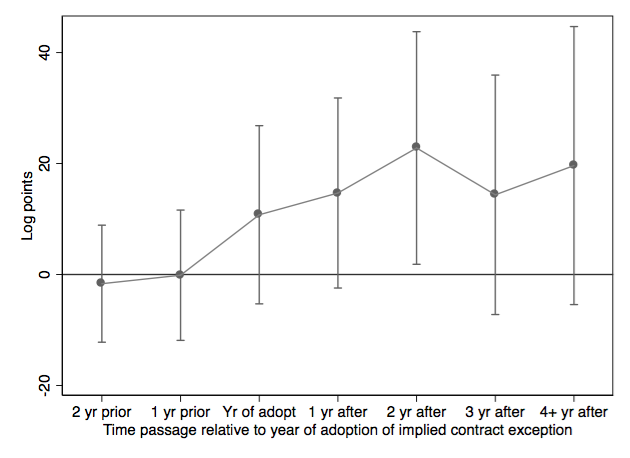
9 |
--------------------------------------------------------------------------------
/03 Making Regression Make Sense/Table 3-3-3.do:
--------------------------------------------------------------------------------
1 | clear all
2 | set more off
3 | eststo clear
4 | capture version 13
5 | /* Required programs */
6 | /* - estout: output table */
7 |
8 | /* Stata code for Table 3.3.2*/
9 |
10 | /* Download data */
11 | shell curl -o nswre74.dta http://economics.mit.edu/files/3828
12 | shell curl -o cps1re74.dta http://economics.mit.edu/files/3824
13 | shell curl -o cps3re74.dta http://economics.mit.edu/files/3825
14 |
15 | /* End of script */
16 |
--------------------------------------------------------------------------------
/02 The Experimental Ideal/Table 2-2-1.do:
--------------------------------------------------------------------------------
1 | clear all
2 | set more off
3 | eststo clear
4 | capture version 13
5 |
6 | /* Pull data from the 'Mostly Harmless' website */
7 | /* http://economics.mit.edu/faculty/angrist/data1/mhe/krueger */
8 | shell curl -o webstar.dta http://economics.mit.edu/files/3827/
9 |
10 | /* Load downloaded data */
11 | use webstar.dta, clear
12 |
13 | /* Create variables in table */
14 | gen white_asian = (inlist(srace, 1, 3)) if !missing(srace)
15 | label var white_asian "White/Asian"
16 |
17 | /* Calculate percentiles of test scores */
18 | local testscores "treadssk tmathssk treadss1 tmathss1 treadss2 tmathss2 treadss3 tmathss3"
19 | foreach var of varlist `testscores' {
20 | xtile pct_`var' = `var', nq(100)
21 | }
22 | egen avg_pct = rowmean(pct_*)
23 | label var avg_pct "Percentile score in kindergarten"
24 |
25 | /* End of file */
26 | exit
27 |
--------------------------------------------------------------------------------
/04 Instrumental Variables in Action/Figure 4-1-1.jl:
--------------------------------------------------------------------------------
1 | # Load packages
2 | using DataFrames
3 | using Gadfly
4 | using GLM
5 |
6 | # Download the data and unzip it
7 | download("http://economics.mit.edu/files/397", "asciiqob.zip")
8 | run(`unzip -o asciiqob.zip`)
9 |
10 | # Import data
11 | pums = readtable("asciiqob.txt",
12 | header = false,
13 | separator = ' ')
14 | names!(pums, [:lwklywge, :educ, :yob, :qob, :pob])
15 |
16 | # Aggregate into means for figure
17 | means = aggregate(pums, [:yob, :qob], [mean])
18 |
19 | # Create dates
20 | means[:date] = [Date(1900 + y, m * 3, 1) for (y, m) in zip(means[:yob], means[:qob])]
21 |
22 | # Plot
23 | p = plot(means,
24 | layer(x = "date", y = "educ_mean", Geom.point, Geom.line))
25 | p = plot(means,
26 | layer(x = "date", y = "lwklywge_mean", Geom.point, Geom.line))
27 |
28 | # End of file
29 |
--------------------------------------------------------------------------------
/07 Quantile Regression/07 Quantile Regression.md:
--------------------------------------------------------------------------------
1 | # 07 Quantile Regression
2 | ## 7.1 The Quantile Regression Model
3 |
4 | ### Table 7.1.1
5 | Completed in [Stata](Table%207-1-1.do), [R](Table%207-1-1.r) and [Python](Table%207-1-1.py)
6 |
7 | | |Obs |Mean |Std Dev |0.1 |0.25 |0.5 |0.75 |0.9 |OLS |RMSE |
8 | |:----|:------|:----|:-------|:-----|:-----|:-----|:-----|:-----|:-----|:----|
9 | |1980 |65,023 |6.4 |0.671 |0.073 |0.073 |0.068 |0.07 |0.079 |0.072 |0.63 |
10 | | | | | |0.002 |0.001 |0.001 |0.001 |0.002 |0.001 | |
11 | |1990 |86,785 |6.46 |0.694 |0.112 |0.11 |0.106 |0.111 |0.137 |0.114 |0.64 |
12 | | | | | |0.003 |0.001 |0.001 |0.001 |0.002 |0.001 | |
13 | |2000 |97,397 |6.47 |0.746 |0.092 |0.105 |0.111 |0.119 |0.157 |0.114 |0.69 |
14 | | | | | |0.003 |0.001 |0.001 |0.001 |0.002 |0.001 | |
15 |
--------------------------------------------------------------------------------
/04 Instrumental Variables in Action/Table 4-1-2.do:
--------------------------------------------------------------------------------
1 | clear all
2 | set more off
3 | /* Stata code for Table 4-1-2 */
4 | /* Required additional packages */
5 | /* - estout: output results */
6 |
7 | * /* Download data */
8 | * shell curl -o asciiqob.zip http://economics.mit.edu/files/397
9 | * unzipfile asciiqob.zip, replace
10 |
11 | /* Import data */
12 | infile lwklywge educ yob qob pob using asciiqob.txt, clear
13 |
14 | /* Create binary instrument */
15 | recode qob (1/2 = 0 "Born in the 1st or 2nd quarter of year") ///
16 | (3/4 = 1 "Born in the 3rd or 4th quarter of year") ///
17 | (else = .), gen(z)
18 |
19 | /* Compare means (and differences) */
20 | ttest lwklywge, by(z)
21 | ttest educ, by(z)
22 |
23 | /* Compute Wald estimate */
24 | sureg (educ z) (lwklywge z) if !missing(z)
25 | nlcom [lwklywge]_b[z] / [educ]_b[z]
26 |
27 | /* OLS estimate */
28 | regress lwklywge educ if !missing(z)
29 |
30 | /* End of script */
31 |
--------------------------------------------------------------------------------
/03 Making Regression Make Sense/Figure 3-1-3.do:
--------------------------------------------------------------------------------
1 | clear all
2 | set more off
3 | eststo clear
4 | capture log close _all
5 | capture version 13
6 |
7 | /* Stata code for Table 3.3.2*/
8 | /* !! Can't find right data !! */
9 |
10 | /* Download data */
11 | * shell curl -o asciiqob.zip http://economics.mit.edu/files/397
12 | * unzipfile asciiqob.zip, replace
13 |
14 | /* Import data */
15 | infile lwklywge educ yob qob pob using asciiqob.txt, clear
16 |
17 | /* Panel A */
18 | /* Old-fashioned standard errors */
19 | regress lwklywge educ
20 | /* Robust standard errors */
21 | regress lwklywge educ, robust
22 |
23 | /* Collapse data for Panel B (counting only if in sample) */
24 | gen count = 1 if e(sample)
25 | collapse (sum) count (mean) lwklywge, by(educ)
26 |
27 | /* Old-fashioned standard errors */
28 | regress lwklywge educ [aweight = count]
29 | /* Robust standard errors */
30 | regress lwklywge educ [aweight = count], robust
31 |
32 | /* End of file */
33 | exit
34 |
--------------------------------------------------------------------------------
/06 Getting a Little Jumpy/06 Getting a Little Jumpy.md:
--------------------------------------------------------------------------------
1 | # 06 Getting a Little Jumpy
2 | ## 6.1 Sharp RD
3 |
4 | ### Figure 6-1-1
5 |
6 | Completed in [Stata](Figure%206-1-1.do), [R](Figure%206-1-1.r), [Python](Figure%206-1-1.py) and [Julia](Figure%206-1-1.jl)
7 |
8 | 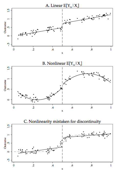
9 |
10 | ### Figure 6-1-2
11 |
12 | Completed in [Stata](Figure%206-1-2.do), [R](Figure%206-1-2.r), [Python](Figure%206-1-2.py) and [Julia](Figure%206-1-2.jl)
13 |
14 | 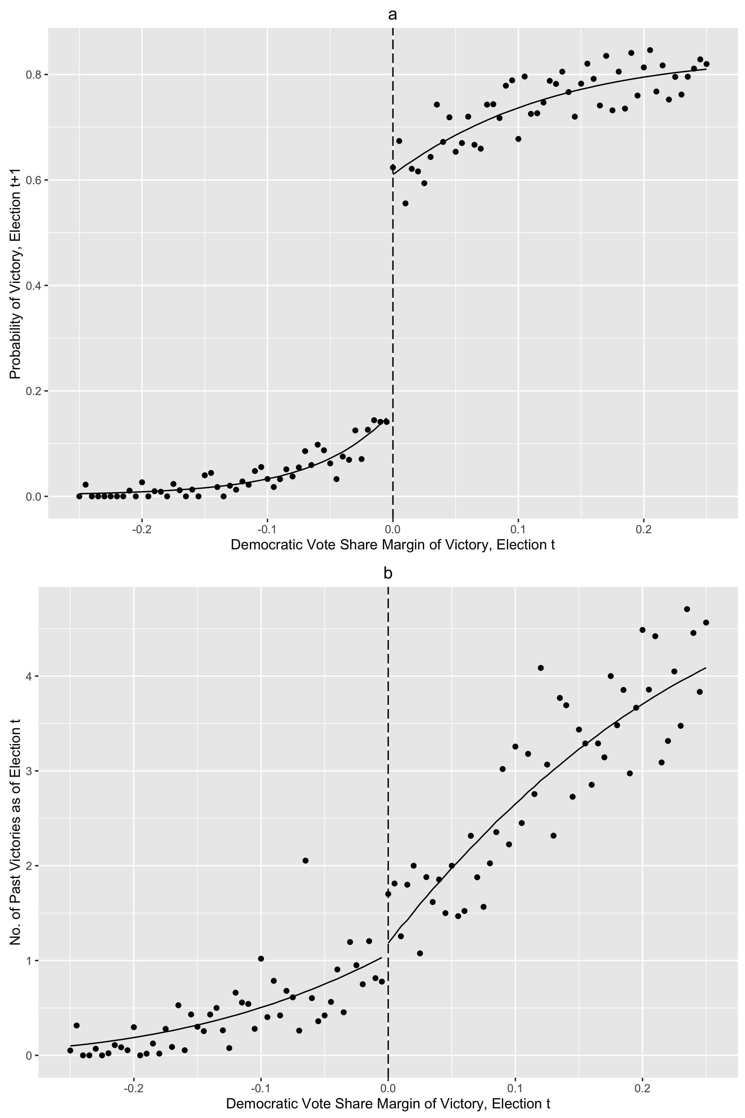
15 |
16 | ### Figure 6-2-1
17 |
18 | Completed in [Stata](Figure%206-2-1.do), [R](Figure%206-2-1.r), [Python](Figure%206-2-1.py) and [Julia](Figure%206-1-1.jl)
19 |
20 | 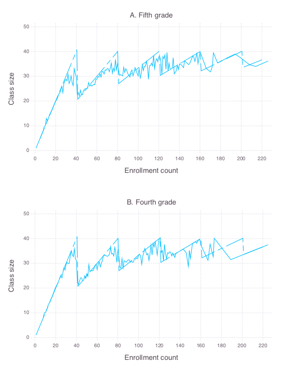
21 |
--------------------------------------------------------------------------------
/07 Quantile Regression/Table 7-1-1.jl:
--------------------------------------------------------------------------------
1 | # Julia code for Table 8-1-1 #
2 | # Required packages #
3 | # - DataRead: import Stata datasets #
4 | # - DataFrames: data manipulation / storage #
5 | # - QuantileRegression: quantile regression #
6 | # - GLM: OLS regression #
7 | using DataRead
8 | using DataFrames
9 | using QuantileRegression
10 | using GLM
11 |
12 | # Download the data and unzip it
13 | download("http://economics.mit.edu/files/384", "angcherfer06.zip")
14 | run(`unzip angcherfer06.zip`)
15 |
16 | # Load the data
17 | dta_path = string("Data/census", "80", ".csv")
18 | df = readtable(dta_path)
19 |
20 | # Summary statistics
21 | obs = size(df[:logwk], 1)
22 | μ = mean(df[:logwk])
23 | σ = std(df[:logwk])
24 |
25 | # Run OLS
26 | wls = glm(logwk ~ educ + black + exper + exper2, df,
27 | Normal(), IdentityLink(),
28 | wts = convert(Array, (df[:perwt])))
29 | wls_coef = coef(wls)[2]
30 | wls_se = stderr(wls)[2]
31 | wls_rmse = sqrt(sum((df[:logwk] - predict(wls)).^2) / df_residual(wls))
32 |
33 | # Print results
34 | print(obs, μ, σ, wls_coef, wls_se, wls_rmse)
35 |
36 | # End of script
37 |
--------------------------------------------------------------------------------
/03 Making Regression Make Sense/Figure 3-1-2.jl:
--------------------------------------------------------------------------------
1 | # Load packages
2 | using CSV
3 | using DataFrames
4 | using GLM
5 | using Statistics
6 | using Gadfly
7 | using Cairo
8 |
9 | # Download the data and unzip it
10 | download("http://economics.mit.edu/files/397", "asciiqob.zip")
11 | run(`unzip asciiqob.zip`)
12 |
13 | # Import data
14 | pums = DataFrame(CSV.File("asciiqob.txt", header = false, delim = " ", ignorerepeated = true))
15 | rename!(pums, [:lwklywge, :educ, :yob, :qob, :pob])
16 |
17 | # Run OLS and save predicted values
18 | OLS = lm(@formula(lwklywge ~ educ), pums)
19 | pums.predicted = predict(OLS)
20 |
21 | # Aggregate into means for figure
22 | means = combine(groupby(pums, :educ), [:lwklywge, :predicted] .=> mean)
23 |
24 | # Plot figure and export figure using Gadfly
25 | figure = plot(means,
26 | layer(x = "educ", y = "predicted_mean", Geom.line, Theme(default_color = colorant"green")),
27 | layer(x = "educ", y = "lwklywge_mean", Geom.line, Geom.point),
28 | Guide.xlabel("Years of completed education"),
29 | Guide.ylabel("Log weekly earnings, \$2003"))
30 |
31 | draw(PNG("Figure 3-1-2-Julia.png", 7inch, 6inch), figure)
32 |
33 | # End of script
34 |
--------------------------------------------------------------------------------
/05 Fixed Effects, DD and Panel Data/Table 5-2-1.do:
--------------------------------------------------------------------------------
1 | clear all
2 | set more off
3 | eststo clear
4 | capture version 13
5 |
6 | /* Stata code for Table 5.2.1*/
7 | shell curl -o njmin.zip http://economics.mit.edu/files/3845
8 | unzipfile njmin.zip, replace
9 |
10 | /* Import data */
11 | infile SHEET CHAIN CO_OWNED STATE SOUTHJ CENTRALJ NORTHJ PA1 PA2 ///
12 | SHORE NCALLS EMPFT EMPPT NMGRS WAGE_ST INCTIME FIRSTINC BONUS ///
13 | PCTAFF MEALS OPEN HRSOPEN PSODA PFRY PENTREE NREGS NREGS11 ///
14 | TYPE2 STATUS2 DATE2 NCALLS2 EMPFT2 EMPPT2 NMGRS2 WAGE_ST2 ///
15 | INCTIME2 FIRSTIN2 SPECIAL2 MEALS2 OPEN2R HRSOPEN2 PSODA2 PFRY2 ///
16 | PENTREE2 NREGS2 NREGS112 using "public.dat", clear
17 |
18 | /* Label the state variables and values */
19 | label var STATE "State"
20 | label define state_labels 0 "PA" 1 "NJ"
21 | label values STATE state_labels
22 |
23 | /* Calculate FTE employement */
24 | gen FTE = EMPFT + 0.5 * EMPPT + NMGRS
25 | label var FTE "FTE employment before"
26 | gen FTE2 = EMPFT2 + 0.5 * EMPPT2 + NMGRS2
27 | label var FTE2 "FTE employment after"
28 |
29 | /* Calculate means */
30 | tabstat FTE FTE2, by(STATE) stat(mean semean)
31 |
32 | /* End of script */
33 |
--------------------------------------------------------------------------------
/06 Getting a Little Jumpy/Table 6-2-1.do:
--------------------------------------------------------------------------------
1 | clear all
2 | set more off
3 | /* Stata code for Figure 5.2.4 */
4 |
5 | /* Download data */
6 | shell curl -o final4.dta http://economics.mit.edu/files/1359
7 | shell curl -o final5.dta http://economics.mit.edu/files/1358
8 |
9 | /* Import data */
10 | use "final5.dta", clear
11 |
12 | replace avgverb= avgverb-100 if avgverb>100
13 | replace avgmath= avgmath-100 if avgmath>100
14 |
15 | gen func1 = c_size / (floor((c_size - 1) / 40) + 1)
16 | gen func2 = cohsize / (floor(cohsize / 40) + 1)
17 |
18 | replace avgverb = . if verbsize == 0
19 | replace passverb = . if verbsize == 0
20 |
21 | replace avgmath = . if mathsize == 0
22 | replace passmath = . if mathsize == 0
23 |
24 | /* Sample restrictions */
25 | keep if 1 < classize & classize < 45 & c_size > 5
26 | keep if c_leom == 1 & c_pik < 3
27 |
28 | sum avgverb
29 | sum avgmath
30 |
31 | mmoulton avgverb classize, cluvar(schlcode)
32 | mmoulton avgverb classize tipuach, cluvar(schlcode)
33 | mmoulton avgverb classize tipuach c_size, clu(schlcode)
34 | mmoulton avgmath classize, cluvar(schlcode)
35 | mmoulton avgmath classize tipuach, cluvar(schlcode)
36 | mmoulton avgmath classize tipuach c_size, clu(schlcode)
37 |
38 | /* End of script */
39 | exit
40 |
--------------------------------------------------------------------------------
/03 Making Regression Make Sense/Figure 3-1-2.do:
--------------------------------------------------------------------------------
1 | clear all
2 | set more off
3 | eststo clear
4 | capture log close _all
5 | capture version 13
6 |
7 | /* Stata code for Table 3.1.2 */
8 | /* Required additional packages */
9 | log using "Table 3-1-2-Stata.txt", name(table030102) text replace
10 |
11 | /* Download data */
12 | shell curl -o asciiqob.zip http://economics.mit.edu/files/397
13 | unzipfile asciiqob.zip, replace
14 |
15 | /* Import data */
16 | infile lwklywge educ yob qob pob using asciiqob.txt, clear
17 |
18 | /* Get fitted line */
19 | regress lwklywge educ
20 | predict yhat, xb
21 |
22 | /* Calculate means by collapsing the data */
23 | collapse lwklywge yhat, by(educ)
24 |
25 | /* Graph the figures */
26 | graph twoway (connected lwklywge educ, lcolor(black) mcolor(black)) ///
27 | (line yhat educ, lcolor(black) lpattern("-")), ///
28 | ylabel(4.8(0.2)6.6) ymtick(4.9(0.2)6.5) ///
29 | xlabel(0(2)20) xmtick(1(2)19) ///
30 | ytitle("Log weekly earnings, $2003") ///
31 | xtitle("Years of completed education") ///
32 | legend(off) ///
33 | scheme(s1mono)
34 |
35 | graph export "Figure 3-1-2-Stata.pdf", replace
36 |
37 | log close table030102
38 | /* End of file */
39 |
--------------------------------------------------------------------------------
/03 Making Regression Make Sense/Figure 3-1-2.r:
--------------------------------------------------------------------------------
1 | # R code for Figure 3.1.2 #
2 | # Required packages #
3 | # - ggplot2: making pretty graphs #
4 | # - data.table: simple way to aggregate #
5 | library(ggplot2)
6 | library(data.table)
7 |
8 | # Download data and unzip the data
9 | download.file('http://economics.mit.edu/files/397', 'asciiqob.zip')
10 | unzip('asciiqob.zip')
11 |
12 | # Read the data into a dataframe
13 | pums <- read.table('asciiqob.txt',
14 | header = FALSE,
15 | stringsAsFactors = FALSE)
16 | names(pums) <- c('lwklywge', 'educ', 'yob', 'qob', 'pob')
17 |
18 | # Estimate OLS regression
19 | reg.model <- lm(lwklywge ~ educ, data = pums)
20 |
21 | # Calculate means by educ attainment and predicted values
22 | pums.data.table <- data.table(pums)
23 | educ.means <- pums.data.table[ , list(mean = mean(lwklywge)), by = educ]
24 | educ.means$yhat <- predict(reg.model, educ.means)
25 |
26 | # Create plot
27 | p <- ggplot(data = educ.means, aes(x = educ)) +
28 | geom_point(aes(y = mean)) +
29 | geom_line(aes(y = mean)) +
30 | geom_line(aes(y = yhat)) +
31 | ylab("Log weekly earnings, $2003") +
32 | xlab("Years of completed education")
33 |
34 | ggsave(filename = "Figure 3-1-2-R.pdf")
35 |
36 |
37 | # End of file
38 |
--------------------------------------------------------------------------------
/04 Instrumental Variables in Action/Table 4-1-2.py:
--------------------------------------------------------------------------------
1 | #!/usr/bin/env python
2 | """
3 | Create Table 4-1-2 in MHE
4 | Tested on Python 3.4
5 | """
6 |
7 | import zipfile
8 | import urllib.request
9 | import pandas as pd
10 | import scipy.stats
11 | import statsmodels.api as sm
12 |
13 | # Download data and unzip the data
14 | urllib.request.urlretrieve('http://economics.mit.edu/files/397', 'asciiqob.zip')
15 | with zipfile.ZipFile('asciiqob.zip', "r") as z:
16 | z.extractall()
17 |
18 | # Read the data into a pandas dataframe
19 | pums = pd.read_csv('asciiqob.txt',
20 | header = None,
21 | delim_whitespace = True)
22 | pums.columns = ['lwklywge', 'educ', 'yob', 'qob', 'pob']
23 |
24 | # Create binary variable
25 | pums['z'] = ((pums.educ == 3) | (pums.educ == 4)) * 1
26 |
27 | # Compare means (and differences)
28 | ttest_lwklywge = scipy.stats.ttest_ind(pums.lwklywge[pums.z == 1], pums.lwklywge[pums.z == 0])
29 | ttest_educ = scipy.stats.ttest_ind(pums.educ[pums.z == 1], pums.educ[pums.z == 0])
30 |
31 | # Compute Wald estimate (need to use arrays to use SUR in statsmodels)
32 | wald_estimate = (np.mean(pums.lwklywge[pums.z == 1]) - np.mean(pums.lwklywge[pums.z == 0])) / \
33 | (np.mean(pums.educ[pums.z == 1]) - np.mean(pums.educ[pums.z == 0]))
34 |
35 | # OLS estimate
36 | ols = sm.OLS(y, X).fit()
37 |
38 | # End of script
39 |
--------------------------------------------------------------------------------
/04 Instrumental Variables in Action/Table 4-1-1.do:
--------------------------------------------------------------------------------
1 | clear all
2 | set more off
3 | /* Stata code for Table 4-1-1 */
4 |
5 | /* Download data */
6 | shell curl -o asciiqob.zip http://economics.mit.edu/files/397
7 | unzipfile asciiqob.zip, replace
8 |
9 | /* Import data */
10 | infile lwklywge educ yob qob pob using asciiqob.txt, clear
11 |
12 | /* Column 1: OLS */
13 | regress lwklywge educ, robust
14 |
15 | /* Column 2: OLS with YOB, POB dummies */
16 | regress lwklywge educ i.yob i.pob, robust
17 |
18 | /* Column 3: 2SLS with instrument QOB = 1 */
19 | tabulate qob, gen(qob)
20 | ivregress 2sls lwklywge (educ = qob1), robust
21 |
22 | /* Column 4: 2SLS with YOB, POB dummies and instrument QOB = 1 */
23 | ivregress 2sls lwklywge i.yob i.pob (educ = qob1), robust
24 |
25 | /* Column 5: 2SLS with YOB, POB dummies and instrument (QOB = 1 | QOB = 2) */
26 | gen qob1or2 = (inlist(qob, 1, 2)) if !missing(qob)
27 | ivregress 2sls lwklywge i.yob i.pob (educ = qob1or2), robust
28 |
29 | /* Column 6: 2SLS with YOB, POB dummies and full QOB dummies */
30 | ivregress 2sls lwklywge i.yob i.pob (educ = i.qob), robust
31 |
32 | /* Column 7: 2SLS with YOB, POB dummies and full QOB dummies interacted with YOB */
33 | ivregress 2sls lwklywge i.yob i.pob (educ = i.qob#i.yob), robust
34 |
35 | /* Column 8: 2SLS with age, YOB, POB dummies and with full QOB dummies interacted with YOB */
36 | ivregress 2sls lwklywge i.yob i.pob (educ = i.qob#i.yob), robust
37 |
38 | /* End of script */
39 |
--------------------------------------------------------------------------------
/03 Making Regression Make Sense/Figure 3-1-2.py:
--------------------------------------------------------------------------------
1 | #!/usr/bin/env python
2 | """
3 | Tested on Python 3.4
4 | """
5 |
6 | import urllib
7 | import zipfile
8 | import urllib.request
9 | import pandas as pd
10 | import statsmodels.api as sm
11 | import matplotlib.pyplot as plt
12 |
13 | # Download data and unzip the data
14 | urllib.request.urlretrieve('http://economics.mit.edu/files/397', 'asciiqob.zip')
15 | with zipfile.ZipFile('asciiqob.zip', "r") as z:
16 | z.extractall()
17 |
18 | # Read the data into a pandas dataframe
19 | pums = pd.read_csv("asciiqob.txt", header=None, delim_whitespace=True)
20 | pums.columns = ["lwklywge", "educ", "yob", "qob", "pob"]
21 |
22 | # Set up the model
23 | y = pums.lwklywge
24 | X = pums.educ
25 | X = sm.add_constant(X)
26 |
27 | # Save coefficient on education
28 | model = sm.OLS(y, X)
29 | results = model.fit()
30 | educ_coef = results.params[1]
31 | intercept = results.params[0]
32 |
33 | # Calculate means by educ attainment and predicted values
34 | groupbyeduc = pums.groupby("educ")
35 | educ_means = groupbyeduc["lwklywge"].mean().reset_index()
36 | yhat = pd.Series(
37 | intercept + educ_coef * educ_means.index.values, index=educ_means.index.values
38 | )
39 |
40 | # Create plot
41 | plt.figure()
42 | educ_means.plot(kind="line", x="educ", y="lwklywge", style="-o")
43 | yhat.plot()
44 | plt.xlabel("Years of completed education")
45 | plt.ylabel("Log weekly earnings, \\$2003")
46 | plt.legend().set_visible(False)
47 | plt.savefig("Figure 3-1-2-Python.pdf")
48 |
49 | # End of script
50 |
--------------------------------------------------------------------------------
/08 Nonstandard Standard Error Issues/Table 8-1-1-alt.r:
--------------------------------------------------------------------------------
1 | # R code for Table 8-1-1 #
2 | # Required packages #
3 | # - sandwich: robust standard error #
4 | library(sandwich)
5 | library(data.table)
6 | library(knitr)
7 |
8 | # Set seed for replication
9 | set.seed(1984, "L'Ecuyer")
10 |
11 | # Set parameters
12 | NSIMS = 25000
13 | N = 30
14 | r = 0.9
15 | N1 = r * N
16 | sigma = 1
17 |
18 | # Generate random data
19 | dvec <- c(rep(0, N1), rep(1, N - N1))
20 | simulated.data <- data.table(sim = rep(1:NSIMS, each = N),
21 | y = NA,
22 | d = rep(dvec, NSIMS),
23 | epsilon = NA)
24 | simulated.data[ , epsilon := ifelse(d == 1,
25 | rnorm((N - N1) * 25),
26 | rnorm(N1 * NSIMS, sd = sigma))]
27 | simulated.data[ , y := 0 * d + epsilon]
28 |
29 | # Store a list of the standard error types
30 | se.types <- c("const", paste0("HC", 0:3))
31 |
32 | # Create a function to extract standard errors
33 | calculate.se <- function(lm.obj, type) {
34 | sqrt(vcovHC(lm.obj, type = type)[2, 2])
35 | }
36 |
37 | # Function to calculate results
38 | calculateBias <- function(formula) {
39 | lm.sim <- lm(formula)
40 | b1 <- coef(lm.sim)[2]
41 | se.sim <- sapply(se.types, calculate.se, lm.obj = lm.sim)
42 | c(b1, se.sim)
43 | }
44 | simulated.results <- simulated.data[ , as.list(calculateBias(y ~ d)), by = sim]
45 |
46 | # End of script
47 |
--------------------------------------------------------------------------------
/07 Quantile Regression/Table 7-1-1.do:
--------------------------------------------------------------------------------
1 | clear all
2 | set more off
3 |
4 | /* Stata code for Table 7.1.1 */
5 |
6 | /* Download data */
7 | shell curl -o angcherfer06.zip http://economics.mit.edu/files/384
8 | unzipfile angcherfer06.zip, replace
9 |
10 | /* Create matrix to store all the results */
11 | matrix R = J(6, 10, .)
12 | matrix rownames R = 80 80se 90 90se 00 00se
13 | matrix colnames R = Obs Mean SD 10 25 50 75 90 Coef MSE
14 |
15 | /* Loop through the years to get the results */
16 | foreach year in "80" "90" "00" {
17 | /* Load data */
18 | use "Data/census`year'.dta", clear
19 |
20 | /* Summary statistics */
21 | summ logwk
22 | matrix R[rownumb(R, "`year'"), colnumb(R, "Obs")] = r(N)
23 | matrix R[rownumb(R, "`year'"), colnumb(R, "Mean")] = r(mean)
24 | matrix R[rownumb(R, "`year'"), colnumb(R, "SD")] = r(sd)
25 |
26 | /* Define education variables */
27 | gen highschool = 1 if (educ == 12)
28 | gen college = 1 if (educ == 16)
29 |
30 | /* Run quantile regressions */
31 | foreach tau of numlist 10 25 50 75 90 {
32 | qreg logwk educ black exper exper2 [pweight = perwt], q(`tau')
33 | matrix R[rownumb(R, "`year'"), colnumb(R, "`tau'")] = _b[edu]
34 | matrix R[rownumb(R, "`year'se"), colnumb(R, "`tau'")] = _se[edu]
35 | }
36 |
37 | /* Run OLS */
38 | regress logwk educ black exper exper2 [pweight = perwt]
39 | matrix R[rownumb(R, "`year'"), colnumb(R, "Coef")] = _b[edu]
40 | matrix R[rownumb(R, "`year'se"), colnumb(R, "Coef")] = _se[edu]
41 | matrix R[rownumb(R, "`year'"), colnumb(R, "MSE")] = e(rmse)
42 | }
43 |
44 | /* List results */
45 | matlist R
46 |
47 | /* End of file */
48 |
--------------------------------------------------------------------------------
/04 Instrumental Variables in Action/Figure 4-6-1.py:
--------------------------------------------------------------------------------
1 | #!/usr/bin/env python
2 | """
3 | Create Figure 4-6-1 in MHE
4 | Tested on Python 3.4
5 | """
6 |
7 | import pandas as pd
8 | import numpy as np
9 | import statsmodels.api as sm
10 | from statsmodels.sandbox.regression import gmm
11 | import matplotlib.pyplot as plt
12 | import random
13 | import math
14 | from scipy.linalg import eigh
15 |
16 | # Number of simulations
17 | nsims = 10
18 |
19 | # Set seed
20 | random.seed(461)
21 |
22 | # Set parameters
23 | Sigma = [[1.0, 0.8],
24 | [0.8, 1.0]]
25 | mu = [0, 0]
26 | errors = np.random.multivariate_normal(mu, Sigma, 1000)
27 | eta = errors[:, 0]
28 | xi = errors[:, 1]
29 |
30 | # Create Z, x, y
31 | Z = np.random.multivariate_normal([0] * 20, np.identity(20), 1000)
32 | x = 0.1 * Z[: , 0] + xi
33 | y = x + eta
34 | x = sm.add_constant(x)
35 | Z = sm.add_constant(x)
36 |
37 | ols = sm.OLS(y, x).fit().params[1]
38 | # tsls = np.linalg.inv(np.transpose(Z).dot(x)).dot(np.transpose(Z).dot(y))[1]
39 | tsls = gmm.IV2SLS(y, x, Z).fit().params[1]
40 |
41 | def LIML(exogenous, endogenous, instruments):
42 | y = exogenous
43 | x = endogenous
44 | Z = instruments
45 | I = np.eye(y.shape[0])
46 | Mz = I - Z.dot(np.linalg.inv(np.transpose(Z).dot(Z))).dot(np.transpose(Z))
47 | Mx = I - x.dot(np.linalg.inv(np.transpose(x).dot(x))).dot(np.transpose(x))
48 | A = np.transpose(np.hstack((y, x[:,1]))).dot(Mz).dot(np.hstack((y, x[:,1])))
49 | k = 1
50 | beta = np.linalg.inv(np.transpose(Z).dot(I - k * M).dot(Z)).dot(np.transpose(Z).dot(I - k * M)).dot(y)
51 | return
52 |
53 | # End of script
54 |
--------------------------------------------------------------------------------
/06 Getting a Little Jumpy/Figure 6-2-1.py:
--------------------------------------------------------------------------------
1 | #!/usr/bin/env python
2 | """
3 | Create Figure 6.2.1 in MHE
4 | Tested on Python 3.4
5 | numpy: math and stat functions, array
6 | matplotlib: plot figures
7 | """
8 | import numpy as np
9 | import matplotlib.pyplot as plt
10 | import pandas as pd
11 |
12 | # Download data
13 | urllib.request.urlretrieve('http://economics.mit.edu/files/1359', 'final4.dta')
14 | urllib.request.urlretrieve('http://economics.mit.edu/files/1358', 'final5.dta')
15 |
16 | # Read the data into a pandas dataframe
17 | grade4 = pd.read_csv('final4.csv', encoding = 'iso8859_8')
18 | grade5 = pd.read_csv('final5.csv', encoding = 'iso8859_8')
19 |
20 | # Find means class size by grade size
21 | grade4means = grade4.groupby('c_size')['classize'].mean()
22 | grade5means = grade5.groupby('c_size')['classize'].mean()
23 |
24 | # Create grid and function for Maimonides Rule
25 | def maimonides_rule(x):
26 | return x / (np.floor((x - 1)/40) + 1)
27 |
28 | x = np.arange(0, 220, 1)
29 |
30 | # Plot figures
31 | fig = plt.figure()
32 |
33 | ax1 = fig.add_subplot(211)
34 | ax1.plot(grade4means)
35 | ax1.plot(x, maimonides_rule(x), '--')
36 | ax1.set_xticks(range(0, 221, 20))
37 | ax1.set_xlabel("Enrollment count")
38 | ax1.set_ylabel("Class size")
39 | ax1.set_title('B. Fourth grade')
40 |
41 | ax2 = fig.add_subplot(212)
42 | ax2.plot(grade5means)
43 | ax2.plot(x, maimonides_rule(x), '--')
44 | ax2.set_xticks(range(0, 221, 20))
45 | ax2.set_xlabel("Enrollment count")
46 | ax2.set_ylabel("Class size")
47 | ax2.set_title('A. Fifth grade')
48 |
49 | plt.tight_layout()
50 | plt.savefig('Figure 6-2-1-Python.png', dpi = 300)
51 |
52 | # End of script
53 |
--------------------------------------------------------------------------------
/06 Getting a Little Jumpy/Figure 6-2-1.jl:
--------------------------------------------------------------------------------
1 | # Load packages
2 | using DataFrames
3 | using Gadfly
4 |
5 | # Download the data
6 | download("http://economics.mit.edu/files/1359", "final4.dta")
7 | download("http://economics.mit.edu/files/1358", "final5.dta")
8 |
9 | # Load the data
10 | grade4 = readtable("final4.csv");
11 | grade5 = readtable("final5.csv");
12 |
13 | # Find means class size by grade size
14 | grade4 = grade4[[:c_size, :classize]];
15 | grade4means = aggregate(grade4, :c_size, [mean])
16 |
17 | grade5 = grade5[[:c_size, :classize]];
18 | grade5means = aggregate(grade5, :c_size, [mean])
19 |
20 | # Create function for Maimonides Rule
21 | function maimonides_rule(x)
22 | x / (floor((x - 1)/40) + 1)
23 | end
24 |
25 | ticks = collect(0:20:220)
26 | p_grade4 = plot(layer(x = grade4means[:c_size], y = grade4means[:classize_mean], Geom.line),
27 | layer(maimonides_rule, 1, 220, Theme(line_style = Gadfly.get_stroke_vector(:dot))),
28 | Guide.xticks(ticks = ticks),
29 | Guide.xlabel("Enrollment count"),
30 | Guide.ylabel("Class size"),
31 | Guide.title("B. Fourth grade"))
32 |
33 | p_grade5 = plot(layer(x = grade5means[:c_size], y = grade5means[:classize_mean], Geom.line),
34 | layer(maimonides_rule, 1, 220, Theme(line_style = Gadfly.get_stroke_vector(:dot))),
35 | Guide.xticks(ticks = ticks),
36 | Guide.xlabel("Enrollment count"),
37 | Guide.ylabel("Class size"),
38 | Guide.title("A. Fifth grade"))
39 |
40 | draw(PNG("Figure 6-2-1-Julia.png", 6inch, 8inch), vstack(p_grade5, p_grade4))
41 |
42 | # End of script
43 |
--------------------------------------------------------------------------------
/04 Instrumental Variables in Action/04 Instrumental Variables in Action.md:
--------------------------------------------------------------------------------
1 | # 04 Instrumental Variables in Action
2 | ## 4.1 IV and causality
3 |
4 | ### Figure 4-1-1
5 |
6 | Completed in [Stata](Figure%204-1-1.do), [R](Figure%204-1-1.r) and [Python](Figure%204-1-1.py)
7 |
8 | 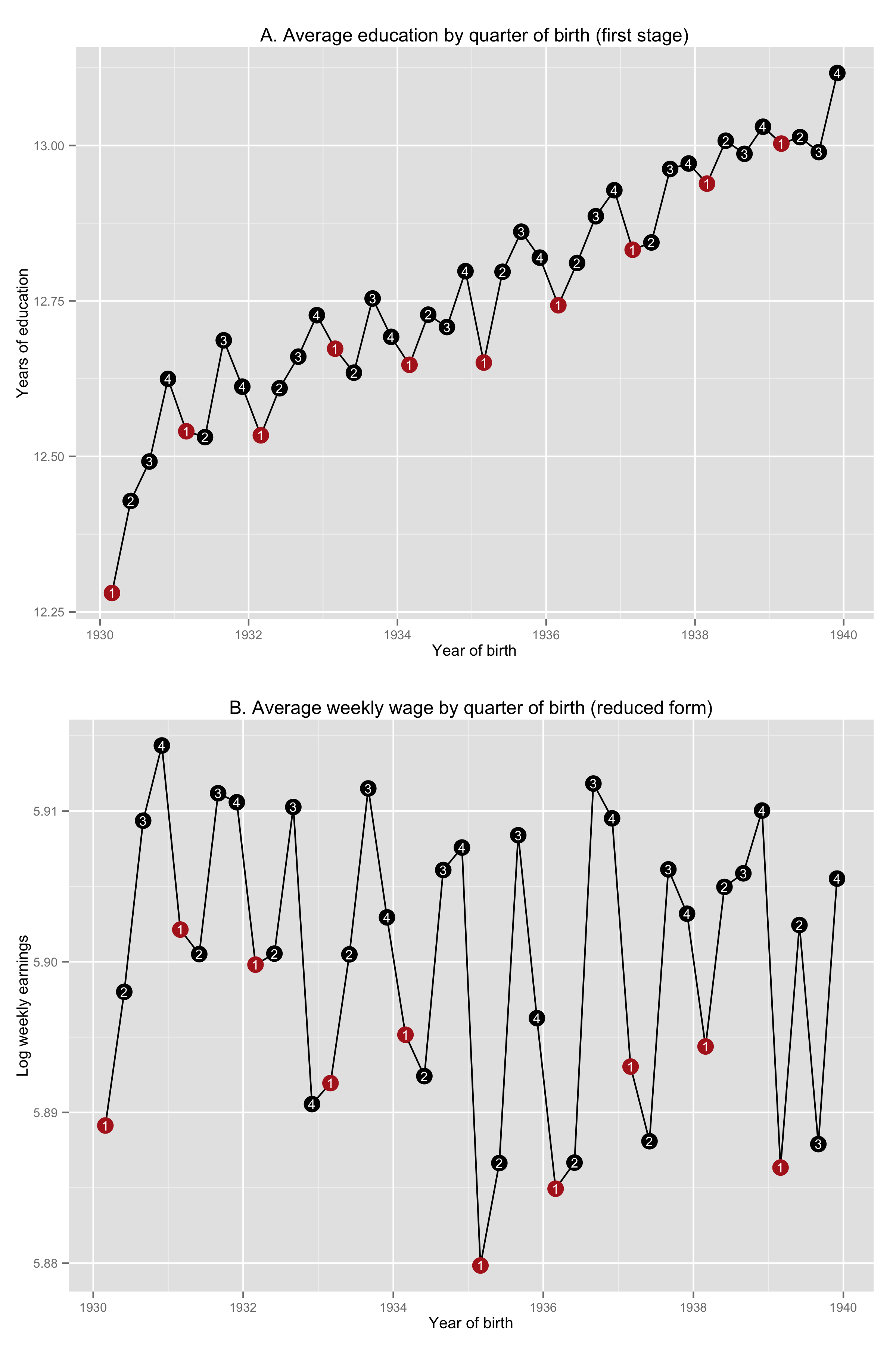
9 |
10 | ### Table 4-1-2
11 |
12 | Completed in [Stata](Table%204-1-2.do) and [R](Table%204-1-2.r)
13 |
14 | | | Born in the 1st or 2nd quarter of year| Born in the 3rd or 4th quarter of year| Difference|
15 | |:------------------|--------------------------------------:|--------------------------------------:|----------:|
16 | |ln(weekly wage) | 5.893844| 5.905829| 0.0119847|
17 | |Years of education | 12.716122| 12.821813| 0.1056907|
18 | |Wald estimate | NA| NA| 0.1133937|
19 | |Wald std error | NA| NA| 0.0215257|
20 | |OLS estimate | NA| NA| 0.0708510|
21 | |OLS std error | NA| NA| 0.0003386|
22 |
23 | ### Figure 4-6-1
24 |
25 | Completed in [Stata](Figure%204-6-1.do) and [R](Figure%204-6-1.r)
26 |
27 | 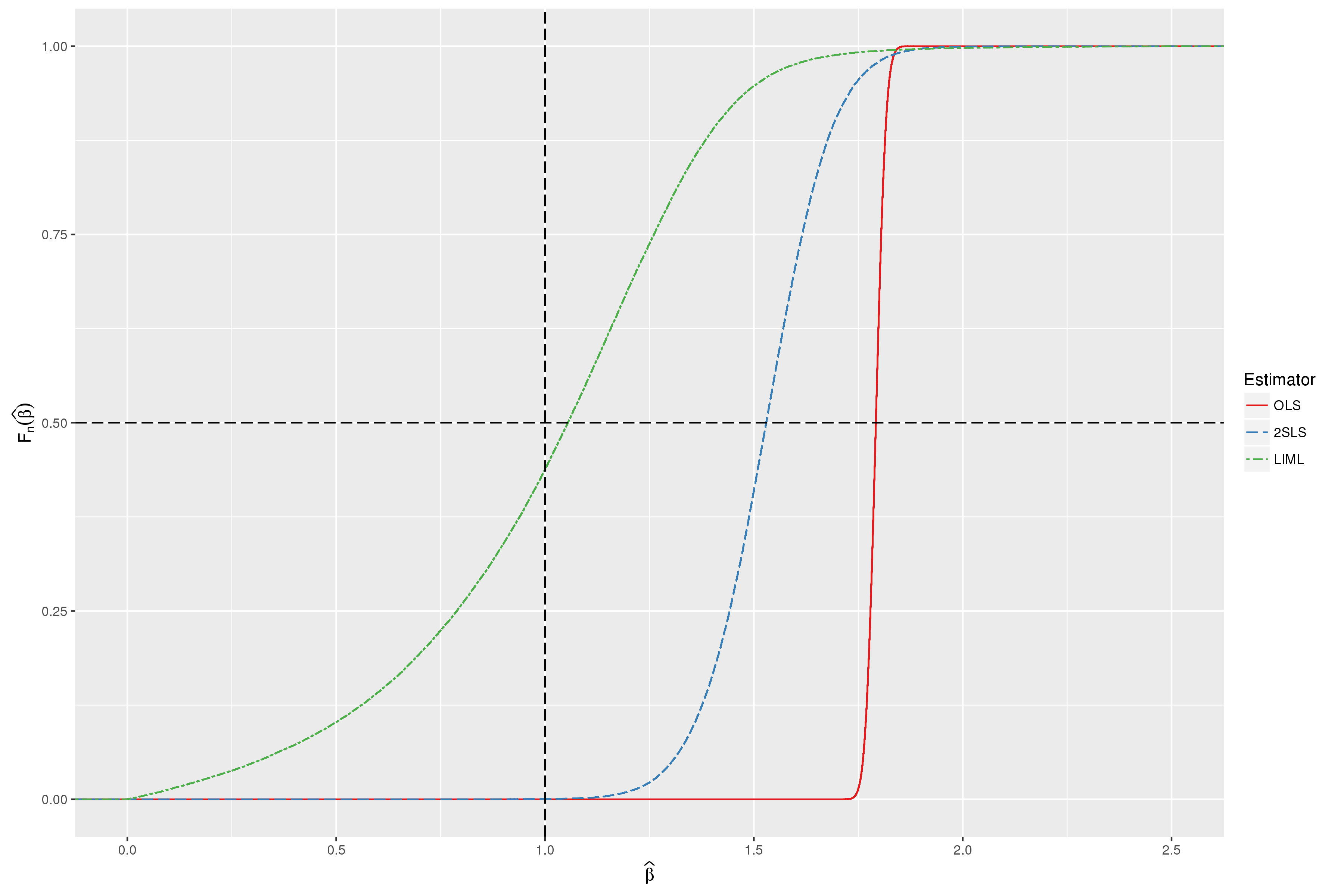
28 |
--------------------------------------------------------------------------------
/03 Making Regression Make Sense/Figure 3-1-3.py:
--------------------------------------------------------------------------------
1 | #!/usr/bin/env python
2 | """
3 | Tested on Python 3.11.5
4 | """
5 |
6 | import urllib
7 | import zipfile
8 | import urllib.request
9 | import pandas as pd
10 | import statsmodels.api as sm
11 | import statsmodels.formula.api as smf
12 |
13 | # Read the data into a pandas.DataFrame
14 | angrist_archive_url = (
15 | 'https://economics.mit.edu/sites/'
16 | 'default/files/publications/asciiqob.zip'
17 | )
18 | pums = pd.read_csv(
19 | angrist_archive_url,
20 | compression = 'zip',
21 | header = None,
22 | sep = '\s+'
23 | )
24 | pums.columns = ['lwklywge', 'educ', 'yob', 'qob', 'pob']
25 |
26 | # Panel A
27 | # Set up the model and fit it
28 | mod_a = smf.ols(
29 | formula = 'lwklywge ~ educ',
30 | data = pums
31 | )
32 | res_a = mod_a.fit()
33 | # Old-fashioned standard errors
34 | print(res_a.summary(title='Old-fashioned standard errors'))
35 | # Robust standard errors
36 | res_a_robust = res_a.get_robustcov_results(cov_type='HC1')
37 | print(
38 | res_a_robust.summary(title='Robust standard errors')
39 | )
40 | # Panel B
41 | # Calculate means and count by educ attainment
42 | pums_agg = pums.groupby('educ').agg(
43 | lwklywge = ('lwklywge', 'mean'),
44 | count = ('lwklywge', 'count')
45 | ).reset_index()
46 | # Set up the model and fit it
47 | mod_b = smf.wls(
48 | formula = 'lwklywge ~ educ',
49 | weights = pums_agg['count'],
50 | data = pums_agg
51 | )
52 | res_b = mod_b.fit()
53 | # Old-fashioned standard errors
54 | print(res_b.summary(title='Old-fashioned standard errors'))
55 | # Robust standard errors
56 | res_b_robust = res_b.get_robustcov_results(cov_type='HC1')
57 | print(
58 | res_b_robust.summary(title='Robust standard errors')
59 | )
60 |
61 | # End of script
62 |
--------------------------------------------------------------------------------
/README.md:
--------------------------------------------------------------------------------
1 | # Mostly Harmless Replication
2 |  3 |
4 | ## Synopsis
5 |
6 | A bold attempt to replicate the tables and figures from the book [_Mostly Harmless Econometrics_](http://www.mostlyharmlesseconometrics.com/) in the following languages:
7 | * Stata
8 | * R
9 | * Python
10 | * Julia
11 |
12 | Why undertake this madness? My primary motivation was to see if I could replace Stata with either R, Python, or Julia in my workflow, so I tried to replicate _Mostly Harmless Econometrics_ in each of these languages.
13 |
14 | ## Chapters
15 | 1. Questions about _Questions_
16 | 2. The Experimental Ideal
17 | 3. [Making Regression Make Sense](03%20Making%20Regression%20Make%20Sense/03%20Making%20Regression%20Make%20Sense.md)
18 | 4. [Instrumental Variables in Action](04%20Instrumental%20Variables%20in%20Action/04%20Instrumental%20Variables%20in%20Action.md)
19 | 5. [Parallel Worlds](05%20Fixed%20Effects%2C%20DD%20and%20Panel%20Data/05%20Fixed%20Effects%2C%20DD%20and%20Panel%20Data.md)
20 | 6. [Getting a Little Jumpy](06%20Getting%20a%20Little%20Jumpy/06%20Getting%20a%20Little%20Jumpy.md)
21 | 7. [Quantile Regression](07%20Quantile%20Regression/07%20Quantile%20Regression.md)
22 | 8. [Nonstandard Standard Error Issues](08%20Nonstandard%20Standard%20Error%20Issues/08%20Nonstanard%20Standard%20Error%20Issues.md)
23 |
24 | ## Getting started
25 | Check out [Getting Started](https://github.com/vikjam/mostly-harmless-replication/wiki/Getting-started) in the Wiki for tips on setting up your machine with each of these languages.
26 |
27 | ## Contributions
28 | Feel free to submit [pull requests](https://github.com/blog/1943-how-to-write-the-perfect-pull-request)!
29 |
30 |
--------------------------------------------------------------------------------
/03 Making Regression Make Sense/Figure 3-1-3.r:
--------------------------------------------------------------------------------
1 | # R code for Figure 3.1.3 #
2 | # Required packages #
3 | # - sandwhich: robust standard errors #
4 | # - lmtest: print table with robust standard errors #
5 | # - data.table: aggregate function #
6 | library(sandwich)
7 | library(lmtest)
8 |
9 | # Download data and unzip the data
10 | download.file('http://economics.mit.edu/files/397', 'asciiqob.zip')
11 | unzip('asciiqob.zip')
12 |
13 | # Read the data into a dataframe
14 | pums <- read.table('asciiqob.txt',
15 | header = FALSE,
16 | stringsAsFactors = FALSE)
17 | names(pums) <- c('lwklywge', 'educ', 'yob', 'qob', 'pob')
18 |
19 | # Panel A
20 | # Estimate OLS regression
21 | reg.model <- lm(lwklywge ~ educ, data = pums)
22 | # Robust standard errors
23 | robust.reg.vcov <- vcovHC(reg.model, "HC1")
24 | # Print results
25 | print(summary(reg.model))
26 | print(coeftest(reg.model, vcov = robust.reg.vcov))
27 |
28 | # Panel B
29 | # Figure out which observations appear in the regression
30 | sample <- !is.na(predict(reg.model, data = pums))
31 | pums.data.table <- data.table(pums[sample, ])
32 | # Aggregate
33 | educ.means <- pums.data.table[ , list(mean = mean(lwklywge),
34 | count = length(lwklywge)),
35 | by = educ]
36 | # Estimate weighted OLS regression
37 | wgt.reg.model <- lm(lwklywge ~ educ,
38 | weights = pums.data.table$count,
39 | data = pums.data.table)
40 | # Robust standard errors with weighted OLS regression
41 | wgt.robust.reg.vcov <- vcovHC(wgt.reg.model, "HC1")
42 | # Print results
43 | print(summary(wgt.reg.model))
44 | print(coeftest(wgt.reg.model, vcov = wgt.reg.vcov))
45 |
46 | # End of file
47 |
--------------------------------------------------------------------------------
/03 Making Regression Make Sense/Table 3-3-2.do:
--------------------------------------------------------------------------------
1 | clear all
2 | set more off
3 | eststo clear
4 | /* Required programs */
5 | /* - estout: output table */
6 |
7 | /* Stata code for Table 3.3.2 */
8 |
9 | * Store URL to MHE Data Archive in local
10 | local base_url = "https://economics.mit.edu/sites/default/files/inline-files"
11 |
12 | /* Store variable list in local */
13 | local summary_var "age ed black hisp nodeg married re74 re75"
14 | local pscore_var "age age2 ed black hisp married nodeg re74 re75"
15 |
16 | /* Columns 1 and 2 */
17 | use "`base_url'/nswre74.dta", clear
18 | eststo column_1, title("NSW Treat"): estpost summarize `summary_var' if treat == 1
19 | eststo column_2, title("NSW Control"): estpost summarize `summary_var' if treat == 0
20 |
21 | /* Column 3 */
22 | use "`base_url'/cps1re74.dta", clear
23 | eststo column_3, title("Full CPS-1"): estpost summarize `summary_var' if treat == 0
24 |
25 | /* Column 5 */
26 | probit treat `pscore_var'
27 | predict p_score, pr
28 | keep if p_score > 0.1 & p_score < 0.9
29 |
30 | eststo column_5, title("P-score CPS-1"): estpost summarize `summary_var' if treat == 0
31 |
32 | /* Column 4 */
33 | use "`base_url'/cps3re74.dta", clear
34 | eststo column_4, title("Full CPS-3"): estpost summarize `summary_var' if treat == 0
35 |
36 | /* Column 6 */
37 | probit treat `pscore_var'
38 | predict p_score, pr
39 | keep if p_score > 0.1 & p_score < 0.9
40 |
41 | eststo column_6, title("P-score CPS-3"): estpost summarize `summary_var' if treat == 0
42 |
43 | /* Label variables */
44 | label var age "Age"
45 | label var ed "Years of Schooling"
46 | label var black "Black"
47 | label var hisp "Hispanic"
48 | label var nodeg "Dropout"
49 | label var married "Married"
50 | label var re74 "1974 earnings"
51 | label var re75 "1975 earnings"
52 |
53 | /* Output Table */
54 | esttab column_1 column_2 column_3 column_4 column_5 column_6, ///
55 | label mtitle ///
56 | cells(mean(label(Mean) fmt(2 2 2 2 2 2 0 0)))
57 |
58 | /* End of script */
59 | exit
60 |
--------------------------------------------------------------------------------
/04 Instrumental Variables in Action/Figure 4-6-1.jl:
--------------------------------------------------------------------------------
1 | # Julia code for Table 4-6-1 #
2 | # Required packages #
3 | # - DataFrames: data manipulation / storage #
4 | # - Distributions: extended stats functions #
5 | # - FixedEffectModels: IV regression #
6 | using DataFrames
7 | using Distributions
8 | using FixedEffectModels
9 | using GLM
10 | using Gadfly
11 |
12 | # Number of simulations
13 | nsims = 1000
14 |
15 | # Set seed
16 | srand(113643)
17 |
18 | # Set parameters
19 | Sigma = [1.0 0.8;
20 | 0.8 1.0]
21 | N = 1000
22 |
23 | function irrelevantInstrMC()
24 | # Create Z, xi and eta
25 | Z = DataFrame(transpose(rand(MvNormal(eye(20)), N)))
26 | errors = DataFrame(transpose(rand(MvNormal(Sigma), N)))
27 |
28 | # Rename columns of Z and errors
29 | names!(Z, [Symbol("z$i") for i in 1:20])
30 | names!(errors, [:eta, :xi])
31 |
32 | # Create y and x
33 | df = hcat(Z, errors);
34 | df[:x] = 0.1 .* df[:z1] .+ df[:xi]
35 | df[:y] = df[:x] .+ df[:eta]
36 |
37 | # Run regressions
38 | ols = coef(lm(@formula(y ~ x), df))[2]
39 | tsls = coef(reg(df, @model(y ~ z1 + z2 + z3 + z4 + z5 + z6 + z7 + z8 + z9 + z10 +
40 | z11 + z12 + z13 + z14 + z15 + z16 + z17 + z18 + z19 + z20)))[2]
41 | return([ols tsls])
42 | end
43 |
44 | # Simulate IV regressions
45 | simulation_results = zeros(nsims, 2);
46 | for i = 1:nsims
47 | simulation_results[i, :] = irrelevantInstrMC()
48 | end
49 |
50 | # Create empirical CDFs from simulated results
51 | ols_ecdf = ecdf(simulation_results[:, 1])
52 | tsls_ecdf = ecdf(simulation_results[:, 2])
53 |
54 | # Plot the empirical CDFs of each estimator
55 | p = plot(layer(ols_ecdf, 0, 2.5, Theme(default_color = colorant"red")),
56 | layer(tsls_ecdf, 0, 2.5, Theme(line_style = :dot)),
57 | layer(xintercept = [0.5], Geom.vline,
58 | Theme(default_color = colorant"black", line_style = :dot)),
59 | layer(yintercept = [0.5], Geom.hline,
60 | Theme(default_color = colorant"black", line_style = :dot)),
61 | Guide.xlabel("Estimated β"),
62 | Guide.ylabel("Fn(Estimated β)"))
63 |
64 | # Export figure as .png
65 | draw(PNG("Figure 4-6-1-Julia.png", 7inch, 6inch), p)
66 |
67 | # End of script
68 |
--------------------------------------------------------------------------------
/06 Getting a Little Jumpy/Figure 6-1-1.py:
--------------------------------------------------------------------------------
1 | #!/usr/bin/env python
2 | """
3 | Create Figure 4-6-1 in MHE
4 | Tested on Python 3.4
5 | numpy: math and stat functions, array
6 | matplotlib: plot figures
7 | """
8 |
9 | import numpy as np
10 | import matplotlib.pyplot as plt
11 |
12 | # Set seed
13 | np.random.seed(10633)
14 |
15 | # Set number of simulations
16 | nobs = 100
17 |
18 | # Generate series
19 | x = np.random.uniform(0, 1, nobs)
20 | x = np.sort(x)
21 | y_linear = x + (x > 0.5) * 0.25 + np.random.normal(0, 0.1, nobs)
22 | y_nonlin = 0.5 * np.sin(6 * (x - 0.5)) + 0.5 + (x > 0.5) * 0.25 + np.random.normal(0, 0.1, nobs)
23 | y_mistake = 1 / (1 + np.exp(-25 * (x - 0.5))) + np.random.normal(0, 0.1, nobs)
24 |
25 | # Fit lines using user-created function
26 | def rdfit(x, y, cutoff, degree):
27 | coef_0 = np.polyfit(x[cutoff >= x], y[cutoff >= x], degree)
28 | fit_0 = np.polyval(coef_0, x[cutoff >= x])
29 |
30 | coef_1 = np.polyfit(x[x > cutoff], y[x > cutoff], degree)
31 | fit_1 = np.polyval(coef_1, x[x > cutoff])
32 |
33 | return coef_0, fit_0, coef_1, fit_1
34 |
35 | coef_y_linear_0 , fit_y_linear_0 , coef_y_linear_1 , fit_y_linear_1 = rdfit(x, y_linear, 0.5, 1)
36 | coef_y_nonlin_0 , fit_y_nonlin_0 , coef_y_nonlin_1 , fit_y_nonlin_1 = rdfit(x, y_nonlin, 0.5, 2)
37 | coef_y_mistake_0, fit_y_mistake_0, coef_y_mistake_1, fit_y_mistake_1 = rdfit(x, y_mistake, 0.5, 1)
38 |
39 | # Plot figures
40 | fig = plt.figure()
41 |
42 | ax1 = fig.add_subplot(311)
43 | ax1.scatter(x, y_linear, edgecolors = 'none')
44 | ax1.plot(x[0.5 >= x], fit_y_linear_0)
45 | ax1.plot(x[x > 0.5], fit_y_linear_1)
46 | ax1.axvline(0.5)
47 | ax1.set_title(r'A. Linear $E[Y_{0i} | X_i]$')
48 |
49 | ax2 = fig.add_subplot(312)
50 | ax2.scatter(x, y_nonlin, edgecolors = 'none')
51 | ax2.plot(x[0.5 >= x], fit_y_nonlin_0)
52 | ax2.plot(x[x > 0.5], fit_y_nonlin_1)
53 | ax2.axvline(0.5)
54 | ax2.set_title(r'B. Nonlinear $E[Y_{0i} | X_i]$')
55 |
56 | ax3 = fig.add_subplot(313)
57 | ax3.scatter(x, y_mistake, edgecolors = 'none')
58 | ax3.plot(x[0.5 >= x], fit_y_mistake_0)
59 | ax3.plot(x[x > 0.5], fit_y_mistake_1)
60 | ax3.plot(x, 1 / (1 + np.exp(-25 * (x - 0.5))), '--')
61 | ax3.axvline(0.5)
62 | ax3.set_title('C. Nonlinearity mistaken for discontinuity')
63 |
64 | plt.tight_layout()
65 | plt.savefig('Figure 6-1-1-Python.png', dpi = 300)
66 |
67 | # End of script
68 |
--------------------------------------------------------------------------------
/04 Instrumental Variables in Action/Table 4-1-1.r:
--------------------------------------------------------------------------------
1 | # R code for Table 4-1-1 #
2 | # Required packages #
3 | # - data.table: data management #
4 | # - sandwich: standard errors #
5 | # - AER: running IV regressions #
6 |
7 | library(data.table)
8 | library(sandwich)
9 | library(AER)
10 |
11 | # Download data and unzip the data
12 | download.file('http://economics.mit.edu/files/397', 'asciiqob.zip')
13 | unzip('asciiqob.zip')
14 |
15 | # Read the data into a data.table
16 | pums <- fread('asciiqob.txt',
17 | header = FALSE,
18 | stringsAsFactors = FALSE)
19 | names(pums) <- c('lwklywge', 'educ', 'yob', 'qob', 'pob')
20 |
21 | # Column 1: OLS
22 | col1 <- lm(lwklywge ~ educ, pums)
23 |
24 | # Column 2: OLS with YOB, POB dummies
25 | col2 <- lm(lwklywge ~ educ + factor(yob) + factor(pob), pums)
26 |
27 | # Create dummies for quarter of birth
28 | qobs <- unique(pums$qob)
29 | qobs.vars <- sapply(qobs, function(x) paste0('qob', x))
30 | pums[, (qobs.vars) := lapply(qobs, function(x) qob == x)]
31 |
32 | # Column 3: 2SLS with instrument QOB = 1
33 | col3 <- ivreg(lwklywge ~ educ, ~ qob1, pums)
34 |
35 | # Column 4: 2SLS with YOB, POB dummies and instrument QOB = 1
36 | col4 <- ivreg(lwklywge ~ factor(yob) + factor(pob) + educ,
37 | ~ factor(yob) + factor(pob) + qob1,
38 | pums)
39 |
40 | # Create dummy for quarter 1 or 2
41 | pums[, qob1or2 := qob == 1 | qob == 2]
42 |
43 | # Column 5: 2SLS with YOB, POB dummies and instrument (QOB = 1 | QOB = 2)
44 | col5 <- ivreg(lwklywge ~ factor(yob) + factor(pob) + educ,
45 | ~ factor(yob) + factor(pob) + qob1or2,
46 | pums)
47 |
48 | # Column 6: 2SLS with YOB, POB dummies and full QOB dummies
49 | col6 <- ivreg(lwklywge ~ factor(yob) + factor(pob) + educ,
50 | ~ factor(yob) + factor(pob) + factor(qob),
51 | pums)
52 |
53 | # Column 7: 2SLS with YOB, POB dummies and full QOB dummies interacted with YOB
54 | col7 <- ivreg(lwklywge ~ factor(yob) + factor(pob) + educ,
55 | ~ factor(pob) + factor(qob) * factor(yob),
56 | pums)
57 |
58 | # Column 8: 2SLS with age, YOB, POB dummies and with full QOB dummies interacted with YOB
59 | col8 <- ivreg(lwklywge ~ factor(yob) + factor(pob) + educ,
60 | ~ factor(pob) + factor(qob) * factor(yob),
61 | pums)
62 |
63 | # End of script
64 |
--------------------------------------------------------------------------------
/04 Instrumental Variables in Action/Figure 4-1-1.py:
--------------------------------------------------------------------------------
1 | #!/usr/bin/env python
2 | """
3 | Create Figure 4-6-1 in MHE
4 | Tested on Python 3.4
5 | """
6 |
7 | import zipfile
8 | import urllib.request
9 | import pandas as pd
10 | import statsmodels.api as sm
11 | import matplotlib.pyplot as plt
12 | from matplotlib.ticker import FormatStrFormatter
13 |
14 | # Download data and unzip the data
15 | urllib.request.urlretrieve('http://economics.mit.edu/files/397', 'asciiqob.zip')
16 | with zipfile.ZipFile('asciiqob.zip', "r") as z:
17 | z.extractall()
18 |
19 | # Read the data into a pandas dataframe
20 | pums = pd.read_csv('asciiqob.txt',
21 | header = None,
22 | delim_whitespace = True)
23 | pums.columns = ['lwklywge', 'educ', 'yob', 'qob', 'pob']
24 |
25 | # Calculate means by educ and lwklywge
26 | groupbybirth = pums.groupby(['yob', 'qob'])
27 | birth_means = groupbybirth['lwklywge', 'educ'].mean()
28 |
29 | # Create function to plot figures
30 | def plot_qob(yvar, ax, title, ylabel):
31 | values = yvar.values
32 | ax.plot(values, color = 'k')
33 |
34 | for i, y in enumerate(yvar):
35 | qob = yvar.index.get_level_values('qob')[i]
36 | ax.annotate(qob,
37 | (i, y),
38 | xytext = (-5, 5),
39 | textcoords = 'offset points')
40 | if qob == 1:
41 | ax.scatter(i, y, marker = 's', facecolors = 'none', edgecolors = 'k')
42 | else:
43 | ax.scatter(i, y, marker = 's', color = 'k')
44 |
45 | ax.set_xticks(range(0, len(yvar), 4))
46 | ax.set_xticklabels(yvar.index.get_level_values('yob')[1::4])
47 | ax.set_title(title)
48 | ax.set_ylabel(ylabel)
49 | ax.yaxis.set_major_formatter(FormatStrFormatter('%.2f'))
50 | ax.set_xlabel("Year of birth")
51 | ax.margins(0.1)
52 |
53 | fig, (ax1, ax2) = plt.subplots(2, sharex = True)
54 |
55 | plot_qob(yvar = birth_means['educ'],
56 | ax = ax1,
57 | title = 'A. Average education by quarter of birth (first stage)',
58 | ylabel = 'Years of education')
59 |
60 | plot_qob(yvar = birth_means['lwklywge'],
61 | ax = ax2,
62 | title = 'B. Average weekly wage by quarter of birth (reduced form)',
63 | ylabel = 'Log weekly earnings')
64 |
65 | fig.tight_layout()
66 | fig.savefig('Figure 4-1-1-Python.pdf', format = 'pdf')
67 |
68 | # End of file
69 |
--------------------------------------------------------------------------------
/06 Getting a Little Jumpy/Figure 6-1-1.r:
--------------------------------------------------------------------------------
1 | # R code for Figure 6-1-1 #
2 | # Required packages #
3 | # - ggplot2: making pretty graphs #
4 | # - gridExtra: combine graphs #
5 | library(ggplot2)
6 | library(gridExtra)
7 |
8 | # Generate series
9 | nobs = 100
10 | x <- runif(nobs)
11 | y.linear <- x + (x > 0.5) * 0.25 + rnorm(n = nobs, mean = 0, sd = 0.1)
12 | y.nonlin <- 0.5 * sin(6 * (x - 0.5)) + 0.5 + (x > 0.5) * 0.25 + rnorm(n = nobs, mean = 0, sd = 0.1)
13 | y.mistake <- 1 / (1 + exp(-25 * (x - 0.5))) + rnorm(n = nobs, mean = 0, sd = 0.1)
14 | rd.series <- data.frame(x, y.linear, y.nonlin, y.mistake)
15 |
16 | # Make graph with ggplot2
17 | g.data <- ggplot(rd.series, aes(x = x, group = x > 0.5))
18 |
19 | p.linear <- g.data + geom_point(aes(y = y.linear)) +
20 | stat_smooth(aes(y = y.linear),
21 | method = "lm",
22 | se = FALSE) +
23 | geom_vline(xintercept = 0.5) +
24 | ylab("Outcome") +
25 | ggtitle(bquote('A. Linear E[' * Y["0i"] * '|' * X[i] * ']'))
26 |
27 | p.nonlin <- g.data + geom_point(aes(y = y.nonlin)) +
28 | stat_smooth(aes(y = y.nonlin),
29 | method = "lm",
30 | formula = y ~ poly(x, 2),
31 | se = FALSE) +
32 | geom_vline(xintercept = 0.5) +
33 | ylab("Outcome") +
34 | ggtitle(bquote('B. Nonlinear E[' * Y["0i"] * '|' * X[i] * ']'))
35 |
36 | f.mistake <- function(x) {1 / (1 + exp(-25 * (x - 0.5)))}
37 | p.mistake <- g.data + geom_point(aes(y = y.mistake)) +
38 | stat_smooth(aes(y = y.mistake),
39 | method = "lm",
40 | se = FALSE) +
41 | stat_function(fun = f.mistake,
42 | linetype = "dashed") +
43 | geom_vline(xintercept = 0.5) +
44 | ylab("Outcome") +
45 | ggtitle('C. Nonlinearity mistaken for discontinuity')
46 |
47 | p.rd.examples <- arrangeGrob(p.linear, p.nonlin, p.mistake, ncol = 1)
48 |
49 | ggsave(p.rd.examples, file = "Figure 6-1-1-R.pdf", width = 5, height = 9)
50 |
51 | # End of script
52 |
--------------------------------------------------------------------------------
/04 Instrumental Variables in Action/Table 4-1-2.r:
--------------------------------------------------------------------------------
1 | # R code for Table 4-1-2 #
2 | # Required packages #
3 | # - data.table: data management #
4 | # - systemfit: SUR #
5 | library(data.table)
6 | library(systemfit)
7 |
8 | # Download data and unzip the data
9 | download.file('http://economics.mit.edu/files/397', 'asciiqob.zip')
10 | unzip('asciiqob.zip')
11 |
12 | # Read the data into a data.table
13 | pums <- fread('asciiqob.txt',
14 | header = FALSE,
15 | stringsAsFactors = FALSE)
16 | names(pums) <- c('lwklywge', 'educ', 'yob', 'qob', 'pob')
17 |
18 | # Create binary variable
19 | pums$z <- (pums$qob == 3 | pums$qob == 4) * 1
20 |
21 | # Compare means (and differences)
22 | ttest.lwklywge <- t.test(lwklywge ~ z, pums)
23 | ttest.educ <- t.test(educ ~ z, pums)
24 |
25 | # Compute Wald estimate
26 | sur <- systemfit(list(first = educ ~ z,
27 | second = lwklywge ~ z),
28 | data = pums,
29 | method = "SUR")
30 | wald <- deltaMethod(sur, "second_z / first_z")
31 |
32 | wald.estimate <- (mean(pums$lwklywge[pums$z == 1]) - mean(pums$lwklywge[pums$z == 0])) /
33 | (mean(pums$educ[pums$z == 1]) - mean(pums$educ[pums$z == 0]))
34 | wald.se <- wald.estimate^2 * ()
35 |
36 | # OLS estimate
37 | ols <- lm(lwklywge ~ educ, pums)
38 |
39 | # Construct table
40 | lwklywge.row <- c(ttest.lwklywge$estimate[1],
41 | ttest.lwklywge$estimate[2],
42 | ttest.lwklywge$estimate[2] - ttest.lwklywge$estimate[1])
43 | educ.row <- c(ttest.educ$estimate[1],
44 | ttest.educ$estimate[2],
45 | ttest.educ$estimate[2] - ttest.educ$estimate[1])
46 | wald.row.est <- c(NA, NA, wald$Estimate)
47 | wald.row.se <- c(NA, NA, wald$SE)
48 |
49 | ols.row.est <- c(NA, NA, summary(ols)$coef['educ' , 'Estimate'])
50 | ols.row.se <- c(NA, NA, summary(ols)$coef['educ' , 'Std. Error'])
51 |
52 | table <- rbind(lwklywge.row, educ.row,
53 | wald.row.est, wald.row.se,
54 | ols.row.est, ols.row.se)
55 | colnames(table) <- c("Born in the 1st or 2nd quarter of year",
56 | "Born in the 3rd or 4th quarter of year",
57 | "Difference")
58 | rownames(table) <- c("ln(weekly wage)",
59 | "Years of education",
60 | "Wald estimate",
61 | "Wald std error",
62 | "OLS estimate",
63 | "OLS std error")
64 |
65 | # End of script
66 |
--------------------------------------------------------------------------------
/08 Nonstandard Standard Error Issues/08 Nonstanard Standard Error Issues.md:
--------------------------------------------------------------------------------
1 | # 08 Nonstandard Standard Error Issues
2 | ## 8.1 The Bias of Robust Standard Errors
3 |
4 | ### Table 8.1.1
5 | Completed in [Stata](Table%208-1-1.do), [R](Table%208-1-1.r), [Python](Table%208-1-1.py) and [Julia](Table%208-1-1.jl)
6 |
7 | _Panel A: Lots of Heteroskedasticity_
8 |
9 | |Estimate | Mean| Std| Normal| t|
10 | |:----------------------|------:|-----:|------:|-----:|
11 | |Beta_1 | -0.006| 0.581| NA| NA|
12 | |Conventional | 0.331| 0.052| 0.269| 0.249|
13 | |HC0 | 0.433| 0.210| 0.227| 0.212|
14 | |HC1 | 0.448| 0.218| 0.216| 0.201|
15 | |HC2 | 0.525| 0.260| 0.171| 0.159|
16 | |HC3 | 0.638| 0.321| 0.124| 0.114|
17 | |max(Conventional, HC0) | 0.461| 0.182| 0.174| 0.159|
18 | |max(Conventional, HC1) | 0.474| 0.191| 0.167| 0.152|
19 | |max(Conventional, HC2) | 0.543| 0.239| 0.136| 0.123|
20 | |max(Conventional, HC3) | 0.650| 0.305| 0.101| 0.091|
21 |
22 | _Panel B: Little Heteroskedasticity_
23 |
24 | |Estimate | Mean| Std| Normal| t|
25 | |:----------------------|------:|-----:|------:|-----:|
26 | |Beta_1 | -0.006| 0.595| NA| NA|
27 | |Conventional | 0.519| 0.070| 0.097| 0.084|
28 | |HC0 | 0.456| 0.200| 0.204| 0.188|
29 | |HC1 | 0.472| 0.207| 0.191| 0.175|
30 | |HC2 | 0.546| 0.251| 0.153| 0.140|
31 | |HC3 | 0.656| 0.312| 0.112| 0.102|
32 | |max(Conventional, HC0) | 0.569| 0.130| 0.081| 0.070|
33 | |max(Conventional, HC1) | 0.577| 0.139| 0.079| 0.067|
34 | |max(Conventional, HC2) | 0.625| 0.187| 0.068| 0.058|
35 | |max(Conventional, HC3) | 0.712| 0.260| 0.054| 0.045|
36 |
37 | _Panel C: No Heteroskedasticity_
38 |
39 | |Estimate | Mean| Std| Normal| t|
40 | |:----------------------|------:|-----:|------:|-----:|
41 | |Beta_1 | -0.006| 0.604| NA| NA|
42 | |Conventional | 0.603| 0.081| 0.059| 0.049|
43 | |HC0 | 0.469| 0.196| 0.193| 0.177|
44 | |HC1 | 0.485| 0.203| 0.180| 0.165|
45 | |HC2 | 0.557| 0.246| 0.145| 0.131|
46 | |HC3 | 0.667| 0.308| 0.106| 0.097|
47 | |max(Conventional, HC0) | 0.633| 0.116| 0.052| 0.043|
48 | |max(Conventional, HC1) | 0.639| 0.123| 0.051| 0.042|
49 | |max(Conventional, HC2) | 0.678| 0.166| 0.045| 0.036|
50 | |max(Conventional, HC3) | 0.752| 0.237| 0.036| 0.030|
51 |
--------------------------------------------------------------------------------
/04 Instrumental Variables in Action/Figure 4-1-1.r:
--------------------------------------------------------------------------------
1 | # R code for Figure 4-1-1 #
2 | # Required packages #
3 | # - dplyr: easy data manipulation #
4 | # - lubridate: data management #
5 | # - ggplot2: making pretty graphs #
6 | # - gridExtra: combine graphs #
7 | library(lubridate)
8 | library(dplyr)
9 | library(ggplot2)
10 | library(gridExtra)
11 |
12 | # Download data and unzip the data
13 | download.file('http://economics.mit.edu/files/397', 'asciiqob.zip')
14 | unzip('asciiqob.zip')
15 |
16 | # Read the data into a dataframe
17 | pums <- read.table('asciiqob.txt',
18 | header = FALSE,
19 | stringsAsFactors = FALSE)
20 | names(pums) <- c('lwklywge', 'educ', 'yob', 'qob', 'pob')
21 |
22 | # Collapse for means
23 | pums.qob.means <- pums %>% group_by(yob, qob) %>% summarise_each(funs(mean))
24 |
25 | # Add dates
26 | pums.qob.means$yqob <- ymd(paste0("19",
27 | pums.qob.means$yob,
28 | pums.qob.means$qob * 3),
29 | truncated = 2)
30 |
31 | # Function for plotting data
32 | plot.qob <- function(ggplot.obj, ggtitle, ylab) {
33 | gg.colours <- c("firebrick", rep("black", 3), "white")
34 | ggplot.obj + geom_line() +
35 | geom_point(aes(colour = factor(qob)),
36 | size = 5) +
37 | geom_text(aes(label = qob, colour = "white"),
38 | size = 3,
39 | hjust = 0.5, vjust = 0.5,
40 | show_guide = FALSE) +
41 | scale_colour_manual(values = gg.colours, guide = FALSE) +
42 | ggtitle(ggtitle) +
43 | xlab("Year of birth") +
44 | ylab(ylab) +
45 | theme_set(theme_gray(base_size = 10))
46 | }
47 |
48 | # Plot
49 | p.educ <- plot.qob(ggplot(pums.qob.means, aes(x = yqob, y = educ)),
50 | "A. Average education by quarter of birth (first stage)",
51 | "Years of education")
52 | p.lwklywge <- plot.qob(ggplot(pums.qob.means, aes(x = yqob, y = lwklywge)),
53 | "B. Average weekly wage by quarter of birth (reduced form)",
54 | "Log weekly earnings")
55 |
56 | p.ivgraph <- arrangeGrob(p.educ, p.lwklywge)
57 |
58 | ggsave(p.ivgraph, file = "Figure 4-1-1-R.png", height = 12, width = 8, dpi = 300)
59 |
60 | # End of script
61 |
--------------------------------------------------------------------------------
/06 Getting a Little Jumpy/Figure 6-2-1.r:
--------------------------------------------------------------------------------
1 | # R code for Figure 6-2-1 #
2 | # Required packages #
3 | # - haven: read Stata .dta files #
4 | # - ggplot2: making pretty graphs #
5 | # - gridExtra: combine graphs #
6 | library(haven)
7 | library(ggplot2)
8 | library(gridExtra)
9 |
10 | # Download the data
11 | download.file("http://economics.mit.edu/files/1359", "final4.dta")
12 | download.file("http://economics.mit.edu/files/1358", "final5.dta")
13 |
14 | # Load the data
15 | grade4 <- read_dta("final4.dta")
16 | grade5 <- read_dta("final5.dta")
17 |
18 | # Restrict sample
19 | grade4 <- grade4[which(grade4$classize & grade4$classize < 45 & grade4$c_size > 5), ]
20 | grade5 <- grade5[which(grade5$classize & grade5$classize < 45 & grade5$c_size > 5), ]
21 |
22 | # Find means class size by grade size
23 | grade4cmeans <- aggregate(grade4$classize,
24 | by = list(grade4$c_size),
25 | FUN = mean,
26 | na.rm = TRUE)
27 | grade5cmeans <- aggregate(grade5$classize,
28 | by = list(grade5$c_size),
29 | FUN = mean,
30 | na.rm = TRUE)
31 |
32 | # Rename aggregaed columns
33 | colnames(grade4cmeans) <- c("c_size", "classize.mean")
34 | colnames(grade5cmeans) <- c("c_size", "classize.mean")
35 |
36 | # Create function for Maimonides Rule
37 | maimonides.rule <- function(x) {x / (floor((x - 1)/40) + 1)}
38 |
39 | # Plot each grade
40 | g4 <- ggplot(data = grade4cmeans, aes(x = c_size))
41 | p4 <- g4 + geom_line(aes(y = classize.mean)) +
42 | stat_function(fun = maimonides.rule,
43 | linetype = "dashed") +
44 | expand_limits(y = 0) +
45 | scale_x_continuous(breaks = seq(0, 220, 20)) +
46 | ylab("Class size") +
47 | xlab("Enrollment count") +
48 | ggtitle("B. Fourth grade")
49 |
50 | g5 <- ggplot(data = grade5cmeans, aes(x = c_size))
51 | p5 <- g5 + geom_line(aes(y = classize.mean)) +
52 | stat_function(fun = maimonides.rule,
53 | linetype = "dashed") +
54 | expand_limits(y = 0) +
55 | scale_x_continuous(breaks = seq(0, 220, 20)) +
56 | ylab("Class size") +
57 | xlab("Enrollment count") +
58 | ggtitle("A. Fifth grade")
59 |
60 | first.stage <- arrangeGrob(p5, p4, ncol = 1)
61 | ggsave(first.stage, file = "Figure 6-2-1-R.png", height = 8, width = 5, dpi = 300)
62 |
63 | # End of script
64 |
--------------------------------------------------------------------------------
/07 Quantile Regression/Table 7-1-1.r:
--------------------------------------------------------------------------------
1 | # R code for Table 7.1.1 #
2 | # Required packages #
3 | # - haven: read in .dta files #
4 | # - quantreg: quantile regressions #
5 | # - knitr: markdown tables #
6 | library(haven)
7 | library(quantreg)
8 | library(knitr)
9 |
10 | # Download data and unzip the data
11 | download.file('http://economics.mit.edu/files/384', 'angcherfer06.zip')
12 | unzip('angcherfer06.zip')
13 |
14 | # Create a function to run the quantile/OLS regressions so we can use a loop
15 | quant.mincer <- function(tau, data) {
16 | r <- rq(logwk ~ educ + black + exper + exper2,
17 | weights = perwt,
18 | data = data,
19 | tau = tau)
20 | return(rbind(summary(r)$coefficients["educ", "Value"],
21 | summary(r)$coefficients["educ", "Std. Error"]))
22 | }
23 |
24 | # Create function for producing the results
25 | calculate.qr <- function(year) {
26 |
27 | # Create file path
28 | dta.path <- paste('Data/census', year, '.dta', sep = "")
29 |
30 | # Load year into the census
31 | df <- read_dta(dta.path)
32 |
33 | # Run quantile regressions
34 | taus <- c(0.1, 0.25, 0.5, 0.75, 0.9)
35 | qr <- sapply(taus, quant.mincer, data = df)
36 |
37 | # Run OLS regressions and get RMSE
38 | ols <- lm(logwk ~ educ + black + exper + exper2,
39 | weights = perwt,
40 | data = df)
41 | coef.se <- rbind(summary(ols)$coefficients["educ", "Estimate"],
42 | summary(ols)$coefficients["educ", "Std. Error"])
43 | rmse <- sqrt(sum(summary(ols)$residuals^2) / ols$df.residual)
44 |
45 | # Summary statistics
46 | obs <- length(na.omit(df$educ))
47 | mean <- mean(df$logwk, na.rm = TRUE)
48 | sd <- sd(df$logwk, na.rm = TRUE)
49 |
50 | return(cbind(rbind(obs, NA),
51 | rbind(mean, NA),
52 | rbind(sd, NA),
53 | qr,
54 | coef.se,
55 | rbind(rmse, NA)))
56 |
57 | }
58 |
59 | # Generate results
60 | results <- rbind(calculate.qr("80"),
61 | calculate.qr("90"),
62 | calculate.qr("00"))
63 |
64 | # Name rows and columns
65 | row.names(results) <- c("1980", "", "1990", "", "2000", "")
66 | colnames(results) <- c("Obs", "Mean", "Std Dev",
67 | "0.1", "0.25", "0.5", "0.75", "0.9",
68 | "OLS", "RMSE")
69 |
70 | # Format decimals
71 | results <- round(results, 3)
72 | results[ , c(2, 10)] <- round(results[ , c(2, 10)], 2)
73 | results[ , 1] <- formatC(results[ , 1], format = "d", big.mark = ",")
74 |
75 | # Export table
76 | print(kable(results))
77 |
78 | # End of file
79 |
--------------------------------------------------------------------------------
/03 Making Regression Make Sense/Table 3-3-2.py:
--------------------------------------------------------------------------------
1 | #!/usr/bin/env python
2 | """
3 | Tested on Python 3.11.13
4 | """
5 |
6 | import urllib.request
7 | import pandas as pd
8 | import statsmodels.api as sm
9 | import numpy as np
10 | import patsy
11 | from tabulate import tabulate
12 |
13 | # Read the Stata files into Python directly from website
14 | base_url = 'https://economics.mit.edu/sites/default/files/inline-files'
15 | nswre74 = pd.read_stata(f"{base_url}/nswre74.dta")
16 | cps1re74 = pd.read_stata(f"{base_url}/cps1re74.dta")
17 | cps3re74 = pd.read_stata(f"{base_url}/cps3re74.dta")
18 |
19 | # Store list of variables for summary
20 | summary_vars = ['age', 'ed', 'black', 'hisp', 'nodeg', 'married', 're74', 're75']
21 |
22 | # Calculate propensity scores
23 | # Create formula for probit
24 | f = 'treat ~ ' + ' + '.join(['age', 'age2', 'ed', 'black', 'hisp', \
25 | 'nodeg', 'married', 're74', 're75'])
26 |
27 | # Run probit with CPS-1
28 | y, X = patsy.dmatrices(f, cps1re74, return_type = 'dataframe')
29 | model = sm.Probit(y, X).fit()
30 | cps1re74['pscore'] = model.predict(X)
31 |
32 | # Run probit with CPS-3
33 | y, X = patsy.dmatrices(f, cps3re74, return_type = 'dataframe')
34 | model = sm.Probit(y, X).fit()
35 | cps3re74['pscore'] = model.predict(X)
36 |
37 | # Create function to summarize data
38 | def summarize(dataset, conditions):
39 | stats = dataset[summary_vars][conditions].mean()
40 | stats['count'] = sum(conditions)
41 | return stats
42 |
43 | # Summarize data
44 | nswre74_treat_stats = summarize(nswre74, nswre74.treat == 1)
45 | nswre74_control_stats = summarize(nswre74, nswre74.treat == 0)
46 | cps1re74_control_stats = summarize(cps1re74, cps1re74.treat == 0)
47 | cps3re74_control_stats = summarize(cps3re74, cps3re74.treat == 0)
48 | cps1re74_ptrim_stats = summarize(cps1re74, (cps1re74.treat == 0) & \
49 | (cps1re74.pscore > 0.1) & \
50 | (cps1re74.pscore < 0.9))
51 | cps3re74_ptrim_stats = summarize(cps3re74, (cps3re74.treat == 0) & \
52 | (cps3re74.pscore > 0.1) & \
53 | (cps3re74.pscore < 0.9))
54 |
55 | # Combine summary stats, add header and print to markdown
56 | frames = [nswre74_treat_stats,
57 | nswre74_control_stats,
58 | cps1re74_control_stats,
59 | cps3re74_control_stats,
60 | cps1re74_ptrim_stats,
61 | cps3re74_ptrim_stats]
62 |
63 | summary_stats = pd.concat(frames, axis = 1)
64 | header = ["NSW Treat", "NSW Control", \
65 | "Full CPS-1", "Full CPS-3", \
66 | "P-score CPS-1", "P-score CPS-3"]
67 |
68 | print(tabulate(summary_stats, header, tablefmt = "pipe"))
69 |
70 | # End of script
71 |
--------------------------------------------------------------------------------
/04 Instrumental Variables in Action/Figure 4-6-1.do:
--------------------------------------------------------------------------------
1 | clear all
2 | set more off
3 | capture log close _all
4 | capture version 13.1 // Note this script has only been tested in Stata 13.1
5 |
6 | /* Stata code for Figure 4.6.1 */
7 |
8 | /* Log output*/
9 | log using "Figure 4-6-1-Stata.txt", name(figure040601) text replace
10 |
11 | /* Set random seed for replication */
12 | set seed 42
13 |
14 | /* Define program for use with -simulate- command */
15 | capture program drop weakinstr
16 | program define weakinstr, rclass
17 | version 13.1
18 |
19 | /* Draw from random normal with correlation of 0.8 and variance of 1 */
20 | matrix C = (1, 0.8 \ 0.8, 1)
21 | quietly drawnorm eta xi, n(1000) corr(C) clear
22 |
23 | /* Create a random instruments */
24 | forvalues i = 1/20 {
25 | quietly gen z`i' = rnormal()
26 | }
27 |
28 | /* Endogenous x only based on z1 while z2-z20 irrelevant */
29 | quietly gen x = 0.1*z1 + xi
30 | quietly gen y = x + eta
31 |
32 | /* OLS */
33 | quietly: regress y x
34 | matrix OLS = e(b)
35 |
36 | /* 2SLS */
37 | quietly: ivregress 2sls y (x = z*)
38 | matrix TSLS = e(b)
39 |
40 | /* LIML */
41 | quietly: ivregress liml y (x = z*)
42 | matrix LIML = e(b)
43 |
44 | /* Return results from program */
45 | return scalar ols = OLS[1, 1]
46 | return scalar tsls = TSLS[1, 1]
47 | return scalar liml = LIML[1, 1]
48 |
49 | end
50 |
51 | /* Run simulation */
52 | simulate coefols = r(ols) coeftsls = r(tsls) coefliml = r(liml), reps(10000): weakinstr
53 |
54 | /* Create empirical CDFs */
55 | cumul coefols, gen(cols)
56 | cumul coeftsls, gen(ctsls)
57 | cumul coefliml, gen(climl)
58 | stack cols coefols ctsls coeftsls climl coefliml, into(c coef) wide clear
59 | label var coef "beta"
60 | label var cols "OLS"
61 | label var ctsls "2SLS"
62 | label var climl "LIML"
63 |
64 | /* Graph results */
65 | graph set window fontface "Palatino"
66 | line cols ctsls climl coef if inrange(coef, 0, 2.5), ///
67 | sort ///
68 | lpattern(solid dash longdash_dot) ///
69 | lwidth(medthick medthick medthick) ///
70 | lcolor("228 26 28" "55 126 184" "77 175 74") ///
71 | scheme(s1color) ///
72 | legend(rows(1) region(lwidth(none))) ///
73 | xline(1, lcolor("189 189 189") lpattern(shortdash) lwidth(medthick)) ///
74 | yline(0.5, lcolor("189 189 189") lpattern(shortdash) lwidth(medthick)) ///
75 | xtitle("estimated {&beta}") ///
76 | ytitle("F{subscript:n}")
77 | graph export "Figure 4-6-1-Stata.eps", replace
78 |
79 | log close figure040601
80 | /* End of script */
81 |
--------------------------------------------------------------------------------
/04 Instrumental Variables in Action/Figure 4-6-1.r:
--------------------------------------------------------------------------------
1 | # R code for Figure 4.6.1 #
2 | # Required packages #
3 | # - MASS: multivariate normal draws #
4 | # - ivmodel: IV regressions #
5 | # - parallel: Parallel process simulation #
6 | # - ggplot2: making pretty graphs #
7 | # - RColorBrewer: pleasing color schemes #
8 | # - reshape: manipulate data #
9 | library(MASS)
10 | library(ivmodel)
11 | library(parallel)
12 | library(ggplot2)
13 | library(RColorBrewer)
14 | library(reshape)
15 |
16 | nsims = 100000
17 | set.seed(1984, "L'Ecuyer")
18 |
19 | irrelevantInstrMC <- function(...) {
20 | # Store coefficients
21 | COEFS <- rep(NA, 3)
22 | names(COEFS) <- c("ols", "tsls", "liml")
23 |
24 | # Set parameters
25 | Sigma = matrix(c(1, 0.8, 0.8, 1), 2, 2)
26 | errors = mvrnorm(n = 1000, rep(0, 2), Sigma)
27 | eta = errors[ , 1]
28 | xi = errors[ , 2]
29 |
30 | # Create Z, x, y
31 | Z = sapply(1:20, function(x) rnorm(1000))
32 | x = 0.1 * Z[ , 1] + xi
33 | y = x + eta
34 |
35 | # OLS
36 | OLS <- lm(y ~ x)
37 | COEFS["ols"] <- summary(OLS)$coefficients[2, 1]
38 |
39 | # Run IV regressions
40 | ivregressions <- ivmodel(Y = y, D = x, Z = Z)
41 | COEFS["tsls"] <- coef.ivmodel(ivregressions)["TSLS", "Estimate"]
42 | COEFS["liml"] <- coef.ivmodel(ivregressions)["LIML", "Estimate"]
43 |
44 | # Return results
45 | return(COEFS)
46 | }
47 |
48 | # Run simulations
49 | SIMBETAS <- data.frame(t(simplify2array(mclapply(1:nsims, irrelevantInstrMC))))
50 |
51 | df <- melt(SIMBETAS[ , 1:3])
52 | names(df) <- c("Estimator", "beta")
53 | df$Estimator <- factor(df$Estimator,
54 | levels = c("ols", "tsls", "liml"),
55 | labels = c("OLS", "2SLS", "LIML"))
56 |
57 | g <- ggplot(df, aes(x = beta, colour = Estimator, linetype = Estimator)) +
58 | stat_ecdf(geom = "step") +
59 | xlab(expression(widehat(beta))) + ylab(expression(F[n](widehat(beta)))) +
60 | xlim(0, 2.5) +
61 | scale_linetype_manual(values = c("solid", "longdash", "twodash")) +
62 | scale_color_manual(values = brewer.pal(3, "Set1"),
63 | labels = c("OLS", "2SLS", "LIML")) +
64 | geom_vline(xintercept = 1.0, linetype = "longdash") +
65 | geom_hline(yintercept = 0.5, linetype = "longdash") +
66 | theme(axis.title.y = element_text(angle=0)) +
67 | theme_set(theme_gray(base_size = 24))
68 | ggsave(file = "Figure 4-6-1-R.png", height = 8, width = 12, dpi = 300)
69 |
70 | write.csv(df, "Figure 4-6-1.csv")
71 | # End of script
72 |
--------------------------------------------------------------------------------
/04 Instrumental Variables in Action/Figure 4-1-1.do:
--------------------------------------------------------------------------------
1 | clear all
2 | set more off
3 | /* Stata code for Figure 4-1-1 */
4 |
5 | /* Download data */
6 | shell curl -o asciiqob.zip http://economics.mit.edu/files/397
7 | unzipfile asciiqob.zip, replace
8 |
9 | /* Import data */
10 | infile lwklywge educ yob qob pob using asciiqob.txt, clear
11 |
12 | /* Use Stata date formats */
13 | gen yqob = yq(1900 + yob, qob)
14 | format yqob %tq
15 |
16 | /* Collapse by quarter of birth */
17 | collapse (mean) educ (mean) lwklywge (mean) qob, by(yqob)
18 |
19 | /* Plot data */
20 | graph twoway (line educ yqob, lcolor(black)) ///
21 | (scatter educ yqob if qob == 1, ///
22 | mlabel(qob) msize(small) msymbol(S) mcolor(black)) ///
23 | (scatter educ yqob if qob != 1, ///
24 | mlabel(qob) msize(small) msymbol(Sh) mcolor(black)), ///
25 | xlabel(, format(%tqY)) ///
26 | title("A. Average education by quarter of birth (first stage)") ///
27 | ytitle("Years of education") ///
28 | xtitle("Year of birth") ///
29 | legend(off) ///
30 | name(educ) ///
31 | scheme(s1mono)
32 |
33 | graph twoway (line lwklywge yqob, lcolor(black)) ///
34 | (scatter lwklywge yqob if qob == 1, ///
35 | mlabel(qob) msize(small) msymbol(S) mcolor(black)) ///
36 | (scatter lwklywge yqob if qob != 1, ///
37 | mlabel(qob) msize(small) msymbol(Sh) mcolor(black)), ///
38 | xlabel(, format(%tqY)) ///
39 | title("B. Average weekly wage by quarter of birth (reduced form)") ///
40 | ytitle("Log weekly earnings") ///
41 | xtitle("Year of birth") ///
42 | legend(off) ///
43 | name(lwklywge) ///
44 | scheme(s1mono)
45 |
46 | /* Compare graphs */
47 | graph combine educ lwklywge, ///
48 | col(1) ///
49 | xsize(4) ysize(6) ///
50 | graphregion(margin(zero)) ///
51 | scheme(s1mono)
52 |
53 | graph export "Figure 4-1-1-Stata.pdf", replace
54 |
55 | /* End of file */
56 |
--------------------------------------------------------------------------------
/06 Getting a Little Jumpy/Figure 6-2-1.do:
--------------------------------------------------------------------------------
1 | clear all
2 | set more off
3 |
4 | /* Download data */
5 | shell curl -o final4.dta http://economics.mit.edu/files/1359
6 | shell curl -o final5.dta http://economics.mit.edu/files/1358
7 |
8 | /*---------*/
9 | /* Grade 4 */
10 | /*---------*/
11 | /* Import data */
12 | use "final4.dta", clear
13 |
14 | /* Restrict sample */
15 | keep if 1 < classize & classize < 45 & c_size > 5
16 |
17 | /* Find means class size by grade size */
18 | collapse classize, by(c_size)
19 |
20 | /* Plot the actual and predicted class size based on grade size */
21 | graph twoway (line classize c_size, lcolor(black)) ///
22 | (function y = x / (floor((x - 1)/40) + 1), ///
23 | range(1 220) lpattern(dash) lcolor(black)), ///
24 | xlabel(20(20)220) ///
25 | title("B. Fourth grade") ///
26 | ytitle("Class size") ///
27 | xtitle("Enrollment count") ///
28 | legend(label(1 "Actual class size") label(2 "Maimonides Rule")) ///
29 | scheme(s1mono) ///
30 | saving(fourthgrade.gph, replace)
31 |
32 | /*---------*/
33 | /* Grade 5 */
34 | /*---------*/
35 | /* Import data */
36 | use "final5.dta", clear
37 |
38 | /* Restrict sample */
39 | keep if 1 < classize & classize < 45 & c_size > 5
40 |
41 | /* Find means class size by grade size */
42 | collapse classize, by(c_size)
43 |
44 | /* Plot the actual and predicted class size based on grade size */
45 | graph twoway (line classize c_size, lcolor(black)) ///
46 | (function y = x / (floor((x - 1)/40) + 1), ///
47 | range(1 220) lpattern(dash) lcolor(black)), ///
48 | xlabel(20(20)220) ///
49 | title("A. Fifth grade") ///
50 | ytitle("Class size") ///
51 | xtitle("Enrollment count") ///
52 | legend(label(1 "Actual class size") label(2 "Maimonides Rule")) ///
53 | scheme(s1mono) ///
54 | saving(fifthgrade.gph, replace)
55 |
56 | /* Combine graphs */
57 | graph combine fifthgrade.gph fourthgrade.gph, ///
58 | col(1) ///
59 | xsize(4) ysize(6) ///
60 | graphregion(margin(zero)) ///
61 | scheme(s1mono)
62 | graph export "Figure 6-2-1-Stata.png", replace
63 |
64 | /* End of file */
65 | exit
66 |
--------------------------------------------------------------------------------
/03 Making Regression Make Sense/Table 3-3-2.jl:
--------------------------------------------------------------------------------
1 | # Load packages
2 | using DataFrames
3 | using FileIO, StatFiles
4 | using Statistics
5 | using GLM
6 |
7 | # Download the data from the MHE Data Archive
8 | base_url = "https://economics.mit.edu/sites/default/files/inline-files"
9 | download("$(base_url)/nswre74.dta", "nswre74.dta")
10 | download("$(base_url)/cps1re74.dta", "cps1re74.dta")
11 | download("$(base_url)/cps3re74.dta", "cps3re74.dta")
12 |
13 | # Read the Stata files into Julia
14 | nswre74 = DataFrame(load("nswre74.dta"))
15 | cps1re74 = DataFrame(load("cps1re74.dta"))
16 | cps3re74 = DataFrame(load("cps3re74.dta"))
17 |
18 | summary_vars = [:age, :ed, :black, :hisp, :nodeg, :married, :re74, :re75]
19 | nswre74_stat = combine(nswre74, summary_vars .=> mean)
20 |
21 | # Calculate propensity scores
22 | probit = glm(@formula(treat ~ age + age2 + ed + black + hisp +
23 | nodeg + married + re74 + re75),
24 | cps1re74,
25 | Binomial(),
26 | ProbitLink())
27 | cps1re74.pscore = predict(probit)
28 |
29 | probit = glm(@formula(treat ~ age + age2 + ed + black + hisp +
30 | nodeg + married + re74 + re75),
31 | cps3re74,
32 | Binomial(),
33 | ProbitLink())
34 | cps3re74.pscore = predict(probit)
35 |
36 | # Create function to summarize data
37 | function summarize(data, condition)
38 | stats = combine(data[condition, :], summary_vars .=> mean)
39 | stats.count = [size(data[condition, summary_vars])[1]]
40 | return(stats)
41 | end
42 |
43 | # Summarize data
44 | nswre74_treat_stats = summarize(nswre74, nswre74.treat .== 1)
45 | nswre74_control_stats = summarize(nswre74, nswre74.treat .== 0)
46 | cps1re74_control_stats = summarize(cps1re74, cps1re74.treat .== 0)
47 | cps3re74_control_stats = summarize(cps3re74, cps3re74.treat .== 0)
48 | cps1re74_ptrim_stats = summarize(cps1re74, broadcast(&, cps1re74.treat .== 0,
49 | cps1re74.pscore .> 0.1,
50 | cps1re74.pscore .< 0.9))
51 | cps3re74_ptrim_stats = summarize(cps3re74, broadcast(&, cps3re74.treat .== 0,
52 | cps3re74.pscore .> 0.1,
53 | cps3re74.pscore .< 0.9))
54 |
55 | # Combine summary stats, add header and print to markdown
56 | table = vcat(nswre74_treat_stats,
57 | nswre74_control_stats,
58 | cps1re74_control_stats,
59 | cps3re74_control_stats,
60 | cps1re74_ptrim_stats,
61 | cps3re74_ptrim_stats)
62 | table.id = 1:size(table, 1)
63 | table = stack(table, [:age_mean, :ed_mean, :black_mean, :hisp_mean,
64 | :nodeg_mean, :married_mean, :re74_mean, :re75_mean, :count])
65 | table = unstack(table, :variable, :id, :value)
66 |
67 | rename!(table, [:Variable, :NSWTreat, :NSWControl,
68 | :FullCPS1, :FullCPS3, :PscoreCPS1, :PscoreCPS3])
69 |
70 | println(table)
71 |
72 | # End of script
73 |
--------------------------------------------------------------------------------
/06 Getting a Little Jumpy/Figure 6-1-1.jl:
--------------------------------------------------------------------------------
1 | # Load packages
2 | using Random
3 | using DataFrames
4 | using Gadfly
5 | using Cairo
6 | using Fontconfig
7 | using Distributions
8 | using CurveFit
9 | using Colors
10 |
11 | # Set seed
12 | Random.seed!(08421);
13 |
14 | # Set number of simulations
15 | nsims = 100
16 |
17 | # Set distributions for random draws
18 | uniform = Uniform(0, 1)
19 | normal = Normal(0, 0.1)
20 |
21 | # Generate series
22 | x = rand(uniform, nsims)
23 | y_linear = x .+ (x .> 0.5) .* 0.25 .+ rand(normal, nsims)
24 | y_nonlin = 0.5 .* sin.(6 .* (x .- 0.5)) .+ 0.5 .+ (x .> 0.5) .* 0.25 .+ rand(normal, nsims)
25 | y_mistake = 1 ./ (1 .+ exp.(-25 .* (x .- 0.5))) .+ rand(normal, nsims)
26 |
27 | # Fit lines using user-created function
28 | function rdfit(xvar, yvar, cutoff, degree)
29 | coef_0 = curve_fit(Poly, xvar[cutoff .>= x], yvar[cutoff .>= x], degree)
30 | fit_0 = coef_0.(xvar[cutoff .>= x])
31 |
32 | coef_1 = curve_fit(Poly, xvar[xvar .> cutoff], yvar[xvar .> cutoff], degree)
33 | fit_1 = coef_1.(xvar[xvar .> cutoff])
34 |
35 | nx_0 = length(xvar[xvar .> cutoff])
36 |
37 | df_0 = DataFrame(x_0 = xvar[cutoff .>= xvar], fit_0 = fit_0)
38 | df_1 = DataFrame(x_1 = xvar[xvar .> cutoff], fit_1 = fit_1)
39 |
40 | return df_0, df_1
41 | end
42 |
43 | data_linear_0, data_linear_1 = rdfit(x, y_linear, 0.5, 1)
44 | data_nonlin_0, data_nonlin_1 = rdfit(x, y_nonlin, 0.5, 2)
45 | data_mistake_0, data_mistake_1 = rdfit(x, y_mistake, 0.5, 1)
46 |
47 | p_linear = plot(layer(x = x, y = y_linear, Geom.point),
48 | layer(x = data_linear_0.x_0, y = data_linear_0.fit_0, Geom.line),
49 | layer(x = data_linear_1.x_1, y = data_linear_1.fit_1, Geom.line),
50 | layer(xintercept = [0.5], Geom.vline),
51 | Guide.xlabel("x"),
52 | Guide.ylabel("Outcome"),
53 | Guide.title("A. Linear E[Y01 | Xi]"))
54 |
55 | p_nonlin = plot(layer(x = x, y = y_nonlin, Geom.point),
56 | layer(x = data_nonlin_0.x_0, y = data_nonlin_0.fit_0, Geom.line),
57 | layer(x = data_nonlin_1.x_1, y = data_nonlin_1.fit_1, Geom.line),
58 | layer(xintercept = [0.5], Geom.vline),
59 | Guide.xlabel("x"),
60 | Guide.ylabel("Outcome"),
61 | Guide.title("B. Nonlinear E[Y01 | Xi]"))
62 |
63 | function rd_mistake(x)
64 | 1 / (1 + exp(-25 * (x - 0.5)))
65 | end
66 |
67 | p_mistake = plot(layer(x = x, y = y_mistake, Geom.point),
68 | layer(x = data_mistake_0.x_0, y = data_mistake_0.fit_0, Geom.line),
69 | layer(x = data_mistake_1.x_1, y = data_mistake_1.fit_1, Geom.line),
70 | layer(rd_mistake, 0, 1),
71 | layer(xintercept = [0.5], Geom.vline),
72 | Guide.xlabel("x"),
73 | Guide.ylabel("Outcome"),
74 | Guide.title("C. Nonlinearity mistaken for discontinuity"))
75 |
76 | draw(PNG("Figure 6-1-1-Julia.png", 6inch, 8inch), vstack(p_linear, p_nonlin, p_mistake))
77 |
78 | # End of script
79 |
--------------------------------------------------------------------------------
/03 Making Regression Make Sense/Table 3-3-3.r:
--------------------------------------------------------------------------------
1 | # R code for Table 3-3-2 #
2 | # Required packages #
3 |
4 | # Download the files
5 | download.file("http://economics.mit.edu/files/3828", "nswre74.dta")
6 | download.file("http://economics.mit.edu/files/3824", "cps1re74.dta")
7 | download.file("http://economics.mit.edu/files/3825", "cps3re74.dta")
8 |
9 | # Read the Stata files into R
10 | nswre74 <- read_dta("nswre74.dta")
11 | cps1re74 <- read_dta("cps1re74.dta")
12 | cps3re74 <- read_dta("cps3re74.dta")
13 |
14 | # Function to create propensity trimmed data
15 | propensity.trim <- function(dataset) {
16 | # Specify control formulas
17 | controls <- c("age", "age2", "ed", "black", "hisp", "nodeg", "married", "re74", "re75")
18 | # Paste together probit specification
19 | spec <- paste("treat", paste(controls, collapse = " + "), sep = " ~ ")
20 | # Run probit
21 | probit <- glm(as.formula(spec), family = binomial(link = "probit"), data = dataset)
22 | # Predict probability of treatment
23 | pscore <- predict(probit, type = "response")
24 | # Return data set within range
25 | dataset[which(pscore > 0.1 & pscore < 0.9), ]
26 | }
27 |
28 | # Propensity trim data
29 | cps1re74.ptrim <- propensity.trim(cps1re74)
30 | cps3re74.ptrim <- propensity.trim(cps3re74)
31 |
32 | estimateTrainingFX <- function(dataset) {
33 | # Raw difference
34 | spec_raw <- as.formula("re78 ~ treat")
35 | coef_raw <- lm(spec_raw, data = dataset)$coefficients["treat"]
36 |
37 | # Demographics
38 | demos <- c("age", "age2", "ed", "black", "hisp", "nodeg", "married")
39 | spec_demo <- paste("re78",
40 | paste(c("treat", demos),
41 | collapse = " + "),
42 | sep = " ~ ")
43 | coef_demo <- lm(spec_demo, data = dataset)$coefficients["treat"]
44 |
45 | # 1975 Earnings
46 | spec_re75 <- paste("re78 ~ treat + re75")
47 | coef_re75 <- lm(spec_demo, data = dataset)$coefficients["treat"]
48 |
49 | # Demographics, 1975 Earnings
50 | spec_demo_re75 <- paste("re78",
51 | paste(c("treat", demos, "re75"),
52 | collapse = " + "),
53 | sep = " ~ ")
54 | coef_demo_re75 <- lm(spec_demo_re75, data = dataset)$coefficients["treat"]
55 |
56 | # Demographics, 1974 and 1975 Earnings
57 | spec_demo_re74_re75 <- paste("re78",
58 | paste(c("treat", demos, "re74", "re75"),
59 | collapse = " + "),
60 | sep = " ~ ")
61 | coef_demo_re74_re75 <- lm(spec_demo_re74_re75, data = dataset)$coefficients["treat"]
62 |
63 | c(raw = coef_raw,
64 | demo = coef_demo,
65 | re75 = coef_re75,
66 | demo_re75 = coef_demo_re75,
67 | demo_re74_re75 = coef_demo_re74_re75)
68 |
69 | }
70 |
71 | nswre74.ols <- estimateTrainingFX(nswre74)
72 | nswre74.ols <- estimateTrainingFX(nswre74)
73 | cps1re74.ols <- estimateTrainingFX(cps1re74)
74 | cps3re74.ols <- estimateTrainingFX(cps3re74)
75 |
76 | # End of script
77 |
--------------------------------------------------------------------------------
/05 Fixed Effects, DD and Panel Data/Table 5-2-1.r:
--------------------------------------------------------------------------------
1 | # R code for Figure 5-2-1 #
2 | # Required packages #
3 | # - dplyr: easy data manipulation #
4 | library(dplyr)
5 |
6 | # Download data
7 | download.file("http://economics.mit.edu/files/3845", "njmin.zip")
8 | unzip("njmin.zip")
9 |
10 | # Import data
11 | njmin <- read.table('public.dat',
12 | header = FALSE,
13 | stringsAsFactors = FALSE,
14 | na.strings = c("", ".", "NA"))
15 | names(njmin) <- c('SHEET', 'CHAIN', 'CO_OWNED', 'STATE', 'SOUTHJ', 'CENTRALJ',
16 | 'NORTHJ', 'PA1', 'PA2', 'SHORE', 'NCALLS', 'EMPFT', 'EMPPT',
17 | 'NMGRS', 'WAGE_ST', 'INCTIME', 'FIRSTINC', 'BONUS', 'PCTAFF',
18 | 'MEALS', 'OPEN', 'HRSOPEN', 'PSODA', 'PFRY', 'PENTREE', 'NREGS',
19 | 'NREGS11', 'TYPE2', 'STATUS2', 'DATE2', 'NCALLS2', 'EMPFT2',
20 | 'EMPPT2', 'NMGRS2', 'WAGE_ST2', 'INCTIME2', 'FIRSTIN2', 'SPECIAL2',
21 | 'MEALS2', 'OPEN2R', 'HRSOPEN2', 'PSODA2', 'PFRY2', 'PENTREE2',
22 | 'NREGS2', 'NREGS112')
23 |
24 | # Calculate FTE employement
25 | njmin$FTE <- njmin$EMPFT + 0.5 * njmin$EMPPT + njmin$NMGRS
26 | njmin$FTE2 <- njmin$EMPFT2 + 0.5 * njmin$EMPPT2 + njmin$NMGRS2
27 |
28 | # Create function for calculating standard errors of mean
29 | semean <- function(x, na.rm = FALSE) {
30 | n <- ifelse(na.rm, sum(!is.na(x)), length(x))
31 | sqrt(var(x, na.rm = na.rm) / n)
32 | }
33 |
34 | # Calucate means
35 | summary.means <- njmin[ , c("FTE", "FTE2", "STATE")] %>%
36 | group_by(STATE) %>%
37 | summarise_each(funs(mean(., na.rm = TRUE)))
38 | summary.means <- as.data.frame(t(summary.means[ , -1]))
39 |
40 | colnames(summary.means) <- c("PA", "NJ")
41 | summary.means$dSTATE <- summary.means$NJ - summary.means$PA
42 | summary.means <- rbind(summary.means,
43 | summary.means[2, ] - summary.means[1, ])
44 | row.names(summary.means) <- c("FTE employment before, all available observations",
45 | "FTE employment after, all available observations",
46 | "Change in mean FTE employment")
47 |
48 | # Calucate
49 | summary.semeans <- njmin[ , c("FTE", "FTE2", "STATE")] %>%
50 | group_by(STATE) %>%
51 | summarise_each(funs(semean(., na.rm = TRUE)))
52 | summary.semeans <- as.data.frame(t(summary.semeans[ , -1]))
53 |
54 | colnames(summary.semeans) <- c("PA", "NJ")
55 | summary.semeans$dSTATE <- sqrt(summary.semeans$NJ + summary.semeans$PA) / length
56 |
57 | njmin <- njmin[ , c("FTE", "FTE2", "STATE")]
58 | njmin <- melt(njmin,
59 | id.vars = c("STATE"),
60 | variable.name = "Period",
61 | value.name = "FTE")
62 | summary.means <- njmin %>%
63 | group_by(STATE, Period) %>%
64 | summarise_each(funs(mean(., na.rm = TRUE), semean(., na.rm = TRUE)))
65 |
66 | # End of script
67 |
--------------------------------------------------------------------------------
/04 Instrumental Variables in Action/Table 4-6-2.do:
--------------------------------------------------------------------------------
1 | clear all
2 | set more off
3 | eststo clear
4 | capture log close _all
5 | capture version 13
6 |
7 | /* Stata code for Table 4.6.2 */
8 | /* Required additional packages */
9 | /* ivreg2: running IV regressions */
10 | /* estout: for exporting tables */
11 |
12 | log using "Table 4-6-2-Stata.txt", name(table040602) text replace
13 |
14 | /* Download data */
15 | shell curl -o asciiqob.zip http://economics.mit.edu/files/397
16 | unzipfile asciiqob.zip, replace
17 |
18 | /* Import data */
19 | infile lwklywge educ yob qob pob using asciiqob.txt, clear
20 |
21 | /*Creat variables */
22 | gen num_qob = yq(1900 + yob, qob) // Quarter of birth
23 | gen survey_qtr = yq(1980, 3) // Survey quarter
24 | gen age = survey_qtr - num_qob // Age in quarter
25 | gen agesq = age^2 // Age^2
26 | xi i.yob i.pob i.qob*i.yob i.qob*i.pob // Create all the dummies
27 |
28 | /* Create locals for controls */
29 | local col1_controls "_Iyob_31 - _Iyob_39"
30 | local col1_excl_instr "_Iqob_2 - _Iqob_4"
31 |
32 | local col2_controls "_Iyob_31 - _Iyob_39 age agesq"
33 | local col2_excl_instr "_Iqob_2 - _Iqob_3" // colinear age qob: drop _Iqob_4
34 |
35 | local col3_controls "_Iyob_31 - _Iyob_39"
36 | local col3_excl_instr "_Iqob_2 - _Iqob_4 _IqobXyob_2_31 - _IqobXyob_4_39"
37 |
38 | local col4_controls "_Iyob_31 - _Iyob_39 age agesq"
39 | local col4_excl_instr "_Iqob_2 - _Iqob_3 _IqobXyob_2_31 - _IqobXyob_4_38" // colinear age qob: drop _Iqob_4, _IqobXyob_4_39
40 |
41 | local col5_controls "_Iyob_31 - _Iyob_39 _Ipob_2 - _Ipob_56"
42 | local col5_excl_instr "_Iqob_2 - _Iqob_4 _IqobXyob_2_31 - _IqobXyob_4_39 _IqobXpob_2_2 - _IqobXpob_4_56"
43 |
44 | local col6_controls "_Iyob_31 - _Iyob_39 _Ipob_2 - _Ipob_56 age agesq"
45 | local col6_excl_instr "_Iqob_2 - _Iqob_3 _IqobXyob_2_31 - _IqobXyob_4_38 _IqobXpob_2_2 - _IqobXpob_4_56" // colinear age qob: drop _Iqob_4, _IqobXyob_4_39
46 |
47 | foreach model in "2sls" "liml" {
48 | if "`model'" == "2sls" {
49 | local ivreg2_mod ""
50 | }
51 | else {
52 | local ivreg2_mod "`model'"
53 | }
54 | foreach col in "col1" "col2" "col3" "col4" "col5" "col6" {
55 | display "Time for `col', `model'"
56 | display "Running ivreg2 lwklywge ``col'_controls' (educ = ``col'_excl_instr'), `ivreg2_mod'"
57 | eststo `col'_`model': ivreg2 lwklywge ``col'_controls' (educ = ``col'_excl_instr'), `ivreg2_mod'
58 | local num_instr = wordcount("`e(exexog)'")
59 | estadd local num_instr `num_instr'
60 | local fstat = round(`e(widstat)', 0.01)
61 | estadd local fstat `fstat'
62 | }
63 | }
64 |
65 | /* OLS for comparison */
66 | eststo col1_ols: regress lwklywge educ i.yob
67 | eststo col2_ols: regress lwklywge educ i.yob age agesq
68 | eststo col5_ols: regress lwklywge educ i.yob i.pob
69 | eststo col6_ols: regress lwklywge educ i.yob i.pob age agesq
70 |
71 | /* Export results */
72 | esttab, keep(educ) ///
73 | b(3) se(3) ///
74 | nostar se noobs mtitles ///
75 | scalars(fstat num_instr) ///
76 | plain replace
77 | eststo clear
78 |
79 | log close table040602
80 | /* End of file */
81 |
--------------------------------------------------------------------------------
/07 Quantile Regression/Table 7-1-1.py:
--------------------------------------------------------------------------------
1 | #!/usr/bin/env python
2 | """
3 | Tested on Python 3.4
4 | """
5 | import urllib
6 | import zipfile
7 | import urllib.request
8 | import pandas as pd
9 | import numpy as np
10 | import statsmodels.api as sm
11 | import statsmodels.formula.api as smf
12 | import matplotlib.pyplot as plt
13 | from statsmodels.regression.quantile_regression import QuantReg
14 | from collections import defaultdict
15 | from tabulate import tabulate
16 |
17 | # Download data and unzip file
18 | urllib.request.urlretrieve('http://economics.mit.edu/files/384', 'angcherfer06.zip')
19 | with zipfile.ZipFile('angcherfer06.zip', 'r') as z:
20 | z.extractall()
21 |
22 | # Function to run the quantile regressions
23 | def quant_mincer(q, data):
24 | r = smf.quantreg('logwk ~ educ + black + exper + exper2 + wt - 1', data)
25 | result = r.fit(q = q)
26 | coef = result.params['educ']
27 | se = result.bse['educ']
28 | return [coef, se]
29 |
30 | # Create dictionary to store the results
31 | results = defaultdict(list)
32 |
33 | # Loop over years and quantiles
34 | years = ['80', '90', '00']
35 | taus = [0.1, 0.25, 0.5, 0.75, 0.9]
36 |
37 | for year in years:
38 | # Load data
39 | dta_path = 'Data/census%s.dta' % year
40 | df = pd.read_stata(dta_path)
41 | # Weight the data by perwt
42 | df['wt'] = np.sqrt(df['perwt'])
43 | wdf = df[['logwk', 'educ', 'black', 'exper', 'exper2']]. \
44 | multiply(df['wt'], axis = 'index')
45 | wdf['wt'] = df['wt']
46 | # Summary statistics
47 | results['Obs'] += [df['logwk'].count(), None]
48 | results['Mean'] += [np.mean(df['logwk']), None]
49 | results['Std'] += [np.std(df['logwk']), None]
50 | # Quantile regressions
51 | for tau in taus:
52 | results[tau] += quant_mincer(tau, wdf)
53 | # Run OLS with weights to get OLS parameters and MSE
54 | wls_model = smf.ols('logwk ~ educ + black + exper + exper2 + wt - 1', wdf)
55 | wls_result = wls_model.fit()
56 | results['OLS'] += [wls_result.params['educ'], wls_result.bse['educ']]
57 | results['RMSE'] += [np.sqrt(wls_result.mse_resid), None]
58 |
59 | # Export table (round the results and place them in a DataFrame to tabulate)
60 | def format_results(the_list, the_format):
61 | return([the_format.format(x) if x else x for x in the_list])
62 |
63 | table = pd.DataFrame(columns = ['Year', 'Obs', 'Mean', 'Std',
64 | '0.1', '0.25', '0.5', '0.75', '0.9',
65 | 'OLS', 'RMSE'])
66 |
67 | table['Year'] = ['1980', None, '1990', None, '2000', None]
68 | table['Obs'] = format_results(results['Obs'], '{:,}')
69 | table['Mean'] = format_results(results['Mean'], '{:.2f}')
70 | table['Std'] = format_results(results['Std'], '{:.3f}')
71 | table['0.1'] = format_results(results[0.1], '{:.3f}')
72 | table['0.25'] = format_results(results[0.25], '{:.3f}')
73 | table['0.5'] = format_results(results[0.5], '{:.3f}')
74 | table['0.75'] = format_results(results[0.75], '{:.3f}')
75 | table['0.9'] = format_results(results[0.9], '{:.3f}')
76 | table['OLS'] = format_results(results['OLS'], '{:.3f}')
77 | table['RMSE'] = format_results(results['RMSE'], '{:.2f}')
78 |
79 | print(tabulate(table, headers = 'keys'))
80 |
81 | # End of script
82 |
--------------------------------------------------------------------------------
/08 Nonstandard Standard Error Issues/Table 8-1-1.jl:
--------------------------------------------------------------------------------
1 | # Julia code for Table 8-1-1 #
2 | # Required packages #
3 | # - DataFrames: data manipulation / storage #
4 | # - Distributions: extended stats functions #
5 | # - GLM: regression #
6 | using DataFrames
7 | using Distributions
8 | using GLM
9 |
10 | # Set seed
11 | srand(08421)
12 |
13 | nsims = 25000
14 |
15 | function generateHC(sigma)
16 | # Set parameters of the simulation
17 | n = 30
18 | r = 0.9
19 | n_1 = int(r * 30)
20 |
21 | # Generate simulation data
22 | d = ones(n)
23 | d[1:n_1] = 0
24 |
25 | r0 = Normal(0, sigma)
26 | r1 = Normal(0, 1)
27 | epsilon = [rand(r0, n_1), rand(r1, n - n_1)]
28 |
29 | y = 0 * d + epsilon
30 |
31 | simulated = DataFrame(y = y, d = d, epsilon = epsilon)
32 |
33 | # Run regression, grab coef., conventional std error, and residuals
34 | regression = lm(y ~ d, simulated)
35 | b1 = coef(regression)[2]
36 | conv = stderr(regression)[2]
37 | ehat = simulated[:y] - predict(regression)
38 |
39 | # Calculate robust standard errors
40 | X = [ones(n) simulated[:d]]
41 | vcovHC0 = inv(transpose(X) * X) * (transpose(X) * diagm(ehat.^2) * X) * inv(transpose(X) * X)
42 | hc0 = sqrt(vcovHC0[2, 2])
43 | vcovHC1 = (n / (n - 2)) * vcovHC0
44 | hc1 = sqrt(vcovHC1[2, 2])
45 | h = diag(X * inv(transpose(X) * X) * transpose(X))
46 | meat2 = diagm(ehat.^2) ./ (1 - h)
47 | vcovHC2 = inv(transpose(X) * X) * (transpose(X) * meat2 * X) * inv(transpose(X) * X)
48 | hc2 = sqrt(vcovHC2[2, 2])
49 | meat3 = diagm(ehat.^2) ./ (1 - h).^2
50 | vcovHC3 = inv(transpose(X) * X) * (transpose(X) * meat3 * X) * inv(transpose(X) * X)
51 | hc3 = sqrt(vcovHC3[2, 2])
52 |
53 | return [b1 conv hc0 hc1 hc2 hc3 max(conv, hc0) max(conv, hc1) max(conv, hc2) max(conv, hc3)]
54 | end
55 |
56 | # Function to run simulation
57 | function simulateHC(nsims, sigma)
58 | # Run simulation
59 | simulation_results = zeros(nsims, 10)
60 |
61 | for i = 1:nsims
62 | simulation_results[i, :] = generateHC(sigma)
63 | end
64 |
65 | # Calculate mean and standard deviation
66 | mean_est = mean(simulation_results, 1)
67 | std_est = std(simulation_results, 1)
68 |
69 | # Calculate rejection rates
70 | test_stats = simulation_results[:, 1] ./ simulation_results[:, 2:10]
71 | reject_z = mean(2 * pdf(Normal(0, 1), -abs(test_stats)) .<= 0.05, 1)
72 | reject_t = mean(2 * pdf(TDist(30 - 2), -abs(test_stats)) .<= 0.05, 1)
73 |
74 | # Combine columns
75 | value_labs = ["Beta_1" "conv" "HC0" "HC1" "HC2" "HC3" "max(conv, HC0)" "max(conv, HC1)" "max(conv, HC2)" "max(conv, HC3)"]
76 | summ_stats = [mean_est; std_est]
77 | reject_stats = [0 reject_z; 0 reject_t]
78 |
79 | all_stats = convert(DataFrame, transpose([value_labs; summ_stats; reject_stats]))
80 | names!(all_stats, [:estimate, :mean, :std, :reject_z, :reject_t])
81 | all_stats[1, 4:5] = NA
82 |
83 | return(all_stats)
84 | end
85 |
86 | println("Panel A")
87 | println(simulateHC(nsims, 0.5))
88 |
89 | println("Panel B")
90 | println(simulateHC(nsims, 0.85))
91 |
92 | println("Panel C")
93 | println(simulateHC(nsims, 1))
94 |
95 | # End of script
96 |
97 |
--------------------------------------------------------------------------------
/06 Getting a Little Jumpy/Figure 6-1-1.do:
--------------------------------------------------------------------------------
1 | clear all
2 | set more off
3 |
4 | /* Set random seed for replication */
5 | set seed 1149
6 |
7 | /* Number of random variables */
8 | local nobs = 100
9 |
10 | set obs `nobs'
11 |
12 | gen x = runiform()
13 | gen y_linear = x + (x > 0.5) * 0.25 + rnormal(0, 0.1)
14 | gen y_nonlin = 0.5 * sin(6 * (x - 0.5)) + 0.5 + (x > 0.5) * 0.25 + rnormal(0, 0.1)
15 | gen y_mistake = 1 / (1 + exp(-25 * (x - 0.5))) + rnormal(0, 0.1)
16 |
17 | graph twoway (lfit y_linear x if x < 0.5, lcolor(black)) ///
18 | (lfit y_linear x if x > 0.5, lcolor(black)) ///
19 | (scatter y_linear x, msize(vsmall) msymbol(circle) mcolor(black)), ///
20 | title("A. Linear E[Y{sub:0i}|X{sub:i}]") ///
21 | ytitle("Outcome") ///
22 | xtitle("x") ///
23 | xline(0.5, lpattern(dash)) ///
24 | scheme(s1mono) ///
25 | legend(off) ///
26 | saving(y_linear, replace)
27 |
28 | graph twoway (qfit y_nonlin x if x < 0.5, lcolor(black)) ///
29 | (qfit y_nonlin x if x > 0.5, lcolor(black)) ///
30 | (scatter y_nonlin x, msize(vsmall) msymbol(circle) mcolor(black)), ///
31 | title("B. Nonlinear E[Y{sub:0i}|X{sub:i}]") ///
32 | ytitle("Outcome") ///
33 | xtitle("x") ///
34 | xline(0.5, lpattern(dash)) ///
35 | scheme(s1mono) ///
36 | legend(off) ///
37 | saving(y_nonlin, replace)
38 |
39 | graph twoway (lfit y_mistake x if x < 0.5, lcolor(black)) ///
40 | (lfit y_mistake x if x > 0.5, lcolor(black)) ///
41 | (function y = 1 / (1 + exp(-25 * (x - 0.5))), lpattern(dash)) ///
42 | (scatter y_mistake x, msize(vsmall) msymbol(circle) mcolor(black)), ///
43 | title("C. Nonlinearity mistaken for discontinuity") ///
44 | ytitle("Outcome") ///
45 | xtitle("x") ///
46 | xline(0.5, lpattern(dash)) ///
47 | scheme(s1mono) ///
48 | legend(off) ///
49 | saving(y_mistake, replace)
50 |
51 | graph combine y_linear.gph y_nonlin.gph y_mistake.gph, ///
52 | col(1) ///
53 | xsize(4) ysize(6) ///
54 | graphregion(margin(zero)) ///
55 | scheme(s1mono)
56 | graph export "Figure 6-1-1-Stata.png", replace
57 |
58 | /* End of file */
59 | exit
60 |
--------------------------------------------------------------------------------
/05 Fixed Effects, DD and Panel Data/Figure 5-2-4.do:
--------------------------------------------------------------------------------
1 | clear all
2 | set more off
3 | eststo clear
4 | capture version 14
5 |
6 | /* Stata code for Figure 5.2.4 */
7 |
8 | /* Download the data and unzip it */
9 | shell curl -o outsourcingatwill_table7.zip "http://economics.mit.edu/~dautor/outsourcingatwill_table7.zip"
10 | unzipfile outsourcingatwill_table7.zip
11 |
12 | /*-------------*/
13 | /* Import data */
14 | /*-------------*/
15 | use "table7/autor-jole-2003.dta", clear
16 |
17 | /* Log total employment: from BLS employment & earnings */
18 | gen lnemp = log(annemp)
19 |
20 | /* Non-business-service sector employment from CBP */
21 | gen nonemp = stateemp - svcemp
22 | gen lnnon = log(nonemp)
23 | gen svcfrac = svcemp / nonemp
24 |
25 | /* Total business services employment from CBP */
26 | gen bizemp = svcemp + peremp
27 | gen lnbiz = log(bizemp)
28 |
29 | /* Time trends */
30 | gen t = year - 78 // Linear time trend
31 | gen t2 = t^2 // Quadratic time trend
32 |
33 | /* Restrict sample */
34 | keep if inrange(year, 79, 95) & state != 98
35 |
36 | /* Generate more aggregate demographics */
37 | gen clp = clg + gtc
38 | gen a1624 = m1619 + m2024 + f1619 + f2024
39 | gen a2554 = m2554 + f2554
40 | gen a55up = m5564 + m65up + f5564 + f65up
41 | gen fem = f1619 + f2024 + f2554 + f5564 + f65up
42 | gen white = rs_wm + rs_wf
43 | gen black = rs_bm + rs_bf
44 | gen other = rs_om + rs_of
45 | gen married = marfem + marmale
46 |
47 | /* Modify union variable */
48 | replace unmem = . if inlist(year, 79, 81) // Don't interpolate 1979, 1981
49 | replace unmem = unmem * 100 // Rescale into percentage
50 |
51 | /* Diff-in-diff regression */
52 | reg lnths lnemp admico_2 admico_1 admico0 admico1 admico2 admico3 mico4 admppa_2 admppa_1 ///
53 | admppa0 admppa1 admppa2 admppa3 mppa4 admgfa_2 admgfa_1 admgfa0 admgfa1 admgfa2 admgfa3 ///
54 | mgfa4 i.year i.state i.state#c.t, cluster(state)
55 |
56 | coefplot, keep(admico_2 admico_1 admico0 admico1 admico2 admico3 mico4) ///
57 | coeflabels(admico_2 = "2 yr prior" ///
58 | admico_1 = "1 yr prior" ///
59 | admico0 = "Yr of adopt" ///
60 | admico1 = "1 yr after" ///
61 | admico2 = "2 yr after" ///
62 | admico3 = "3 yr after" ///
63 | mico4 = "4+ yr after") ///
64 | vertical ///
65 | yline(0) ///
66 | ytitle("Log points") ///
67 | xtitle("Time passage relative to year of adoption of implied contract exception") ///
68 | addplot(line @b @at) ///
69 | ciopts(recast(rcap)) ///
70 | rescale(100) ///
71 | scheme(s1mono)
72 | graph export "Figures/Figure 5-2-4.png", replace
73 |
74 | /* End of script */
75 |
--------------------------------------------------------------------------------
/05 Fixed Effects, DD and Panel Data/Figure 5-2-4.r:
--------------------------------------------------------------------------------
1 | # R code for Figure 5-2-4 #
2 | # Required packages #
3 | # foreign: read Stata .dta files #
4 | # lfe: run fixed effect regressions #
5 | # ggplot2: plot results #
6 | library(foreign)
7 | library(lfe)
8 | library(ggplot2)
9 |
10 | # Download the data and unzip it
11 | download.file(
12 | "https://www.dropbox.com/s/m6o0704ohzwep4s/outsourcingatwill_table7.zip?dl=1",
13 | "outsourcingatwill_table7.zip"
14 | )
15 | unzip("outsourcingatwill_table7.zip")
16 |
17 | # Load the data
18 | autor <- read.dta("table7/autor-jole-2003.dta")
19 |
20 | # Log total employment: from BLS employment & earnings
21 | autor$lnemp <- log(autor$annemp)
22 |
23 | # Non-business-service sector employment from CBP
24 | autor$nonemp <- autor$stateemp - autor$svcemp
25 | autor$lnnon <- log(autor$nonemp)
26 | autor$svcfrac <- autor$svcemp / autor$nonemp
27 |
28 | # Total business services employment from CBP
29 | autor$bizemp <- autor$svcemp + autor$peremp
30 | autor$lnbiz <- log(autor$bizemp)
31 |
32 | # Restrict sample
33 | autor <- autor[which(autor$year >= 79 & autor$year <= 95), ]
34 | autor <- autor[which(autor$state != 98), ]
35 |
36 | # State dummies, year dummies, and state*time trends
37 | autor$t <- autor$year - 78
38 | autor$t2 <- autor$t^2
39 |
40 | # Generate more aggregate demographics
41 | autor$clp <- autor$clg + autor$gtc
42 | autor$a1624 <- autor$m1619 + autor$m2024 + autor$f1619 + autor$f2024
43 | autor$a2554 <- autor$m2554 + autor$f2554
44 | autor$a55up <- autor$m5564 + autor$m65up + autor$f5564 + autor$f65up
45 | autor$fem <- autor$f1619 + autor$f2024 + autor$f2554 + autor$f5564 + autor$f65up
46 | autor$white <- autor$rs_wm + autor$rs_wf
47 | autor$black <- autor$rs_bm + autor$rs_bf
48 | autor$other <- autor$rs_om + autor$rs_of
49 | autor$married <- autor$marfem + autor$marmale
50 |
51 | # Modify union variable (1. Don't interpolate 1979, 1981; 2. Rescale into percentage)
52 | autor$unmem[79 == autor$year | autor$year == 81] <- NA
53 | autor$unmem <- autor$unmem * 100
54 |
55 | # Create state and year factors
56 | autor$state <- factor(autor$state)
57 | autor$year <- factor(autor$year)
58 |
59 | # Diff-in-diff regression
60 | did <- felm(lnths ~ lnemp + admico_2 + admico_1 + admico0 + admico1 + admico2 +
61 | admico3 + mico4 + admppa_2 + admppa_1 + admppa0 + admppa1 +
62 | admppa2 + admppa3 + mppa4 + admgfa_2 + admgfa_1 + admgfa0 +
63 | admgfa1 + admgfa2 + admgfa3 + mgfa4
64 | | state + year + state:t | 0 | state, data = autor)
65 |
66 | # Plot results
67 | lags_leads <- c(
68 | "admico_2", "admico_1", "admico0",
69 | "admico1", "admico2", "admico3",
70 | "mico4"
71 | )
72 | labels <- c(
73 | "2 yr prior", "1 yr prior", "Yr of adopt",
74 | "1 yr after", "2 yr after", "3 yr after",
75 | "4+ yr after"
76 | )
77 | results.did <- data.frame(
78 | label = factor(labels, levels = labels),
79 | coef = summary(did)$coef[lags_leads, "Estimate"] * 100,
80 | se = summary(did)$coef[lags_leads, "Cluster s.e."] * 100
81 | )
82 | g <- ggplot(results.did, aes(label, coef, group = 1))
83 | p <- g + geom_point() +
84 | geom_line(linetype = "dotted") +
85 | geom_pointrange(aes(
86 | ymax = coef + 1.96 * se,
87 | ymin = coef - 1.96 * se
88 | )) +
89 | geom_hline(yintercept = 0) +
90 | ylab("Log points") +
91 | xlab(paste(
92 | "Time passage relative to year of",
93 | "adoption of implied contract exception"
94 | ))
95 |
96 | ggsave(p, file = "Figure 5-2-4-R.png", height = 6, width = 8, dpi = 300)
97 |
98 | # End of script
99 |
--------------------------------------------------------------------------------
/03 Making Regression Make Sense/Table 3-3-2.r:
--------------------------------------------------------------------------------
1 | # R code for Table 3-3-2 #
2 | # Required packages #
3 | # - haven: read .dta files #
4 | # - knitr: print markdown #
5 | library(haven)
6 | library(knitr)
7 |
8 | # Read the Stata files into R directly from MHE Data Archive
9 | base_url = "https://economics.mit.edu/sites/default/files/inline-files"
10 | nswre74 <- read_dta(paste(base_url, "nswre74.dta", sep = "/"))
11 | cps1re74 <- read_dta(paste(base_url, "cps1re74.dta", sep = "/"))
12 | cps3re74 <- read_dta(paste(base_url, "cps3re74.dta", sep = "/"))
13 |
14 | # Function to create propensity trimmed data
15 | propensity.trim <- function(dataset) {
16 | # Specify control formulas
17 | controls <- c("age", "age2", "ed", "black", "hisp", "nodeg", "married", "re74", "re75")
18 | # Paste together probit specification
19 | spec <- paste("treat", paste(controls, collapse = " + "), sep = " ~ ")
20 | # Run probit
21 | probit <- glm(as.formula(spec), family = binomial(link = "probit"), data = dataset)
22 | # Predict probability of treatment
23 | pscore <- predict(probit, type = "response")
24 | # Return data set within range
25 | dataset[which(pscore > 0.1 & pscore < 0.9), ]
26 | }
27 |
28 | # Propensity trim data
29 | cps1re74.ptrim <- propensity.trim(cps1re74)
30 | cps3re74.ptrim <- propensity.trim(cps3re74)
31 |
32 | # Create function for summary statistics
33 | summarize <- function(dataset, treat) {
34 | # Variables to summarize
35 | summary.variables <- c("age", "ed", "black", "hisp", "nodeg", "married", "re74", "re75")
36 | # Calculate mean, removing missing
37 | summary.means <- sapply(dataset[treat, summary.variables], mean, na.rm = TRUE)
38 | summary.count <- sum(treat)
39 | c(summary.means, count = summary.count)
40 | }
41 |
42 | # Summarize data
43 | nswre74.treat.stats <- summarize(nswre74, nswre74$treat == 1)
44 | nswre74.control.stats <- summarize(nswre74, nswre74$treat == 0)
45 | cps1re74.stats <- summarize(cps1re74, cps1re74$treat == 0)
46 | cps3re74.stats <- summarize(cps3re74, cps3re74$treat == 0)
47 | cps1re74.ptrim.stats <- summarize(cps1re74.ptrim, cps1re74.ptrim$treat == 0)
48 | cps3re74.ptrim.stats <- summarize(cps3re74.ptrim, cps3re74.ptrim$treat == 0)
49 |
50 | # Combine the summary statistics
51 | summary.stats <- rbind(nswre74.treat.stats,
52 | nswre74.control.stats,
53 | cps1re74.stats,
54 | cps3re74.stats,
55 | cps1re74.ptrim.stats,
56 | cps3re74.ptrim.stats)
57 |
58 | # Round the digits and transpose table
59 | summary.stats <- cbind(round(summary.stats[ , 1:6], 2),
60 | formatC(round(summary.stats[ , 7:9], 0),
61 | format = "d",
62 | big.mark = ","))
63 | summary.stats <- t(summary.stats)
64 |
65 | # Format table with row and column names
66 | row.names(summary.stats) <- c("Age",
67 | "Years of schooling",
68 | "Black",
69 | "Hispanic",
70 | "Dropout",
71 | "Married",
72 | "1974 earnings",
73 | "1975 earnings",
74 | "Number of Obs.")
75 |
76 | colnames(summary.stats) <- c("NSW Treat", "NSW Control",
77 | "Full CPS-1", "Full CPS-3",
78 | "P-score CPS-1", "P-score CPS-3")
79 |
80 | # Print table in markdown
81 | print(kable(summary.stats))
82 |
83 | # End of script
84 |
--------------------------------------------------------------------------------
/05 Fixed Effects, DD and Panel Data/Figure 5-2-4.jl:
--------------------------------------------------------------------------------
1 | # Load packages
2 | using FileIO, StatFiles, DataFrames, CategoricalArrays
3 | using FixedEffectModels
4 | using Gadfly
5 | using Cairo
6 |
7 | # Download the data and unzip it
8 | download(
9 | "https://www.dropbox.com/s/m6o0704ohzwep4s/outsourcingatwill_table7.zip?dl=1",
10 | "outsourcingatwill_table7.zip",
11 | )
12 | run(`unzip -o outsourcingatwill_table7.zip`)
13 |
14 | # Import data
15 | autor = DataFrame(load("table7/autor-jole-2003.dta"));
16 |
17 | # Log total employment: from BLS employment & earnings
18 | autor.lnemp = log.(autor.annemp);
19 |
20 | # Non-business-service sector employment from CBP
21 | autor.nonemp = autor.stateemp .- autor.svcemp;
22 | autor.lnnon = log.(autor.nonemp);
23 | autor.svcfrac = autor.svcemp ./ autor.nonemp;
24 |
25 | # Total business services employment from CBP
26 | autor.bizemp = autor.svcemp .+ autor.peremp
27 | autor.lnbiz = log.(autor.bizemp)
28 |
29 | # Restrict sample
30 | autor = autor[autor.year.>=79, :];
31 | autor = autor[autor.year.<=95, :];
32 | autor = autor[autor.state.!=98, :];
33 |
34 | # State dummies, year dummies, and state*time trends
35 | autor.t = autor.year .- 78;
36 | autor.t2 = autor.t .^ 2;
37 |
38 | # Generate more aggregate demographics
39 | autor.clp = autor.clg .+ autor.gtc;
40 | autor.a1624 = autor.m1619 .+ autor.m2024 .+ autor.f1619 .+ autor.f2024;
41 | autor.a2554 = autor.m2554 .+ autor.f2554;
42 | autor.a55up = autor.m5564 .+ autor.m65up .+ autor.f5564 .+ autor.f65up;
43 | autor.fem = autor.f1619 .+ autor.f2024 .+ autor.f2554 .+ autor.f5564 .+ autor.f65up;
44 | autor.white = autor.rs_wm .+ autor.rs_wf;
45 | autor.black = autor.rs_bm .+ autor.rs_bf;
46 | autor.other = autor.rs_om .+ autor.rs_of;
47 | autor.married = autor.marfem .+ autor.marmale;
48 |
49 | # Create categorical variable for state and year
50 | autor.state_c = categorical(autor.state);
51 | autor.year_c = categorical(autor.year);
52 |
53 | # Diff-in-diff regression
54 | did = reg(
55 | autor,
56 | @formula(
57 | lnths ~
58 | lnemp +
59 | admico_2 + admico_1 + admico0 + admico1 + admico2 + admico3 + mico4 +
60 | admppa_2 + admppa_1 + admppa0 + admppa1 + admppa2 + admppa3 + mppa4 +
61 | admgfa_2 + admgfa_1 + admgfa0 + admgfa1 + admgfa2 + admgfa3 + mgfa4 +
62 | fe(state_c) + fe(year_c) + fe(state_c)&t
63 | ),
64 | Vcov.cluster(:state_c),
65 | )
66 |
67 | # Store results in a DataFrame for a plot
68 | results_did = DataFrame(
69 | label = coefnames(did),
70 | coef = coef(did) .* 100,
71 | se = stderror(did) .* 100
72 | );
73 |
74 | # Keep only the relevant coefficients
75 | results_did = filter(r -> any(occursin.(r"admico|mico", r.label)), results_did);
76 |
77 | # Define labels for coefficients
78 | results_did.label .= [
79 | "2 yr prior",
80 | "1 yr prior",
81 | "Yr of adopt",
82 | "1 yr after",
83 | "2 yr after",
84 | "3 yr after",
85 | "4+ yr after",
86 | ];
87 |
88 | # Make plot
89 | figure = plot(
90 | results_did,
91 | x = "label",
92 | y = "coef",
93 | ymin = results_did.coef .- 1.96 .* results_did.se,
94 | ymax = results_did.coef .+ 1.96 .* results_did.se,
95 | Geom.point,
96 | Geom.line,
97 | Geom.errorbar,
98 | Guide.xlabel(
99 | "Time passage relative to year of adoption " *
100 | "of implied contract exception",
101 | ),
102 | Guide.ylabel("Log points"),
103 | );
104 |
105 | # Export figure
106 | draw(PNG("Figure 5-2-4-Julia.png", 7inch, 6inch), figure);
107 |
--------------------------------------------------------------------------------
/06 Getting a Little Jumpy/Figure 6-1-2.py:
--------------------------------------------------------------------------------
1 | #!/usr/bin/env python
2 | """
3 | Create Figure 6.1.2 in MHE
4 | Tested on Python 3.4
5 | pandas: import .dta and manipulate data
6 | altair: plot figures
7 | """
8 | import urllib
9 | import zipfile
10 | import urllib.request
11 | import pandas
12 | import matplotlib.pyplot as plt
13 | import seaborn as sns
14 | import numpy
15 | from patsy import dmatrices
16 | from sklearn.linear_model import LogisticRegression
17 |
18 | # Download data and unzip the data
19 | urllib.request.urlretrieve('http://economics.mit.edu/faculty/angrist/data1/mhe/lee', 'Lee2008.zip')
20 | with zipfile.ZipFile('Lee2008.zip', 'r') as z:
21 | z.extractall()
22 |
23 | # Load the data
24 | lee = pandas.read_stata('Lee2008/individ_final.dta')
25 |
26 | # Subset by non-missing in the outcome and running variable for panel (a)
27 | panel_a = lee[['myoutcomenext', 'difshare']].dropna(axis = 0)
28 |
29 | # Create indicator when crossing the cut-off
30 | panel_a['d'] = (panel_a['difshare'] >= 0) * 1.0
31 |
32 | # Create matrices for logistic regression
33 | y, X = dmatrices('myoutcomenext ~ d*(difshare + numpy.power(difshare, 2) + numpy.power(difshare, 3) + numpy.power(difshare, 4))', panel_a)
34 |
35 | # Flatten y into a 1-D array for the sklearn LogisticRegression
36 | y = numpy.ravel(y)
37 |
38 | # Run the logistic regression
39 | logit = LogisticRegression().fit(X, y)
40 |
41 | # Produce predicted probabilities
42 | panel_a['predict'] = logit.predict_proba(X)[:, 1]
43 |
44 | # Create 0.005 intervals of the running variable
45 | breaks = numpy.arange(-1.0, 1.005, 0.005)
46 | panel_a['i005'] = pandas.cut(panel_a['difshare'], breaks)
47 |
48 | # Calculate means by interval
49 | mean_panel_a = panel_a.groupby('i005').mean().dropna(axis = 0)
50 | restriction_a = (mean_panel_a['difshare'] > -0.251) & (mean_panel_a['difshare'] < 0.251)
51 | mean_panel_a = mean_panel_a[restriction_a]
52 |
53 | # Calculate means for panel (b)
54 | panel_b = lee[['difshare', 'mofficeexp', 'mpofficeexp']].dropna(axis = 0)
55 | panel_b['i005'] = pandas.cut(panel_b['difshare'], breaks)
56 | mean_panel_b = panel_b.groupby('i005').mean().dropna(axis = 0)
57 | restriction_b = (mean_panel_b['difshare'] > -0.251) & (mean_panel_b['difshare'] < 0.251)
58 | mean_panel_b = mean_panel_b[restriction_b]
59 |
60 | # Plot figures
61 | fig = plt.figure(figsize = (7, 7))
62 |
63 | # Panel (a)
64 | ax_a = fig.add_subplot(211)
65 | ax_a.scatter(mean_panel_a['difshare'],
66 | mean_panel_a['myoutcomenext'],
67 | edgecolors = 'none', color = 'black')
68 | ax_a.plot(mean_panel_a['difshare'][mean_panel_a['difshare'] >= 0],
69 | mean_panel_a['predict'][mean_panel_a['difshare'] >= 0],
70 | color = 'black')
71 | ax_a.plot(mean_panel_a['difshare'][mean_panel_a['difshare'] < 0],
72 | mean_panel_a['predict'][mean_panel_a['difshare'] < 0],
73 | color = 'black')
74 | ax_a.axvline(0, linestyle = '--', color = 'black')
75 | ax_a.set_title('a')
76 |
77 | # Panel (b)
78 | ax_b = fig.add_subplot(212)
79 | ax_b.scatter(mean_panel_b['difshare'],
80 | mean_panel_b['mofficeexp'],
81 | edgecolors = 'none', color = 'black')
82 | ax_b.plot(mean_panel_b['difshare'][mean_panel_b['difshare'] >= 0],
83 | mean_panel_b['mpofficeexp'][mean_panel_b['difshare'] >= 0],
84 | color = 'black')
85 | ax_b.plot(mean_panel_b['difshare'][mean_panel_b['difshare'] < 0],
86 | mean_panel_b['mpofficeexp'][mean_panel_b['difshare'] < 0],
87 | color = 'black')
88 | ax_b.axvline(0, linestyle = '--', color = 'black')
89 | ax_b.set_title('b')
90 |
91 | plt.tight_layout()
92 | plt.savefig('Figure 6-1-2-Python.png', dpi = 300)
93 |
94 | # End of script
95 |
--------------------------------------------------------------------------------
/06 Getting a Little Jumpy/Figure 6-1-2.r:
--------------------------------------------------------------------------------
1 | # R code for Figure 6.1.2 #
2 | # Required packages #
3 | # - haven: read .dta files #
4 | # - data.table: alternative to data.frame #
5 | # - ggplot2: making pretty graphs #
6 | # - gridExtra: combine graphs #
7 | library(haven)
8 | library(data.table)
9 | library(ggplot2)
10 | library(gridExtra)
11 |
12 | # Download data and unzip the data
13 | # download.file('http://economics.mit.edu/faculty/angrist/data1/mhe/lee', 'Lee2008.zip')
14 | # unzip('Lee2008.zip')
15 |
16 | # Load the .dta file as data.table
17 | lee <- data.table(read_dta('Lee2008/individ_final.dta'))
18 |
19 | # Subset by non-missing in the outcome and running variable for panel (a)
20 | panel.a <- na.omit(lee[, c("myoutcomenext", "difshare"), with = FALSE])
21 |
22 | # Create indicator when crossing the cut-off
23 | panel.a <- panel.a[ , d := (difshare >= 0) * 1.0]
24 |
25 | # Predict with local polynomial logit of degree 4
26 | logit <- glm(formula = myoutcomenext ~ poly(difshare, degree = 4) +
27 | poly(difshare, degree = 4) * d,
28 | family = binomial(link = "logit"),
29 | data = panel.a)
30 | panel.a <- panel.a[ , pmyoutcomenext := predict(logit, panel.a, type = "response")]
31 |
32 | # Create local average by 0.005 interval of the running variable
33 | breaks <- round(seq(-1, 1, by = 0.005), 3)
34 | panel.a <- panel.a[ , i005 := as.numeric(as.character(cut(difshare,
35 | breaks = breaks,
36 | labels = head(breaks, -1),
37 | right = TRUE))), ]
38 |
39 | panel.a <- panel.a[ , list(m_next = mean(myoutcomenext),
40 | mp_next = mean(pmyoutcomenext)),
41 | by = i005]
42 |
43 | # Plot panel (a)
44 | panel.a <- panel.a[which(panel.a$i005 > -0.251 & panel.a$i005 < 0.251), ]
45 | plot.a <- ggplot(data = panel.a, aes(x = i005)) +
46 | geom_point(aes(y = m_next)) +
47 | geom_line(aes(y = mp_next, group = i005 >= 0)) +
48 | geom_vline(xintercept = 0, linetype = 'longdash') +
49 | xlab('Democratic Vote Share Margin of Victory, Election t') +
50 | ylab('Probability of Victory, Election t+1') +
51 | ggtitle('a')
52 |
53 | # Subset the outcome for panel (b)
54 | panel.b <- lee[ , i005 := as.numeric(as.character(cut(difshare,
55 | breaks = breaks,
56 | labels = head(breaks, -1),
57 | right = TRUE))), ]
58 |
59 | panel.b <- panel.b[ , list(m_vic = mean(mofficeexp, na.rm = TRUE),
60 | mp_vic = mean(mpofficeexp, na.rm = TRUE)),
61 | by = i005]
62 |
63 | panel.b <- panel.b[which(panel.b$i005 > -0.251 & panel.b$i005 < 0.251), ]
64 | plot.b <- ggplot(data = panel.b, aes(x = i005)) +
65 | geom_point(aes(y = m_vic)) +
66 | geom_line(aes(y = mp_vic, group = i005 >= 0)) +
67 | geom_vline(xintercept = 0, linetype = 'longdash') +
68 | xlab('Democratic Vote Share Margin of Victory, Election t') +
69 | ylab('No. of Past Victories as of Election t') +
70 | ggtitle('b')
71 |
72 | lee.p <- arrangeGrob(plot.a, plot.b)
73 | ggsave(lee.p, file = "Figure 6-1-2-R.png", height = 12, width = 8, dpi = 300)
74 |
75 | # End of script
76 |
--------------------------------------------------------------------------------
/05 Fixed Effects, DD and Panel Data/Figure 5-2-4.py:
--------------------------------------------------------------------------------
1 | #!/usr/bin/env python
2 | """
3 | Tested on Python 3.8.5
4 | """
5 | import urllib.request
6 | import zipfile
7 | import pandas as pd
8 | import numpy as np
9 | from linearmodels.panel import PanelOLS
10 | import seaborn as sns
11 | import matplotlib.pyplot as plt
12 |
13 | # Download data and unzip the data
14 | urllib.request.urlretrieve('https://www.dropbox.com/s/m6o0704ohzwep4s/outsourcingatwill_table7.zip?dl=1', 'outsourcingatwill_table7.zip')
15 | with zipfile.ZipFile('outsourcingatwill_table7.zip', 'r') as z:
16 | z.extractall()
17 |
18 | # Import data
19 | autor = pd.read_stata("table7/autor-jole-2003.dta")
20 |
21 | # Log total employment: from BLS employment & earnings
22 | autor["lnemp"] = np.log(autor["annemp"])
23 |
24 | # Non-business-service sector employment from CBP
25 | autor["nonemp"] = autor["stateemp"] - autor["svcemp"]
26 | autor["lnnon"] = np.log(autor["nonemp"])
27 | autor["svcfrac"] = autor["svcemp"] / autor["nonemp"]
28 |
29 | # Total business services employment from CBP
30 | autor["bizemp"] = autor["svcemp"] + autor["peremp"]
31 | autor["lnbiz"] = np.log(autor["bizemp"])
32 |
33 | # Restrict sample
34 | autor = autor[autor["year"] >= 79]
35 | autor = autor[autor["year"] <= 95]
36 | autor = autor[autor["state"] != 98]
37 |
38 | # State dummies, year dummies, and state*time trends
39 | autor["t"] = autor["year"] - 78
40 | autor["t2"] = autor["t"] ** 2
41 |
42 | # Generate more aggregate demographics
43 | autor["clp"] = autor["clg"] + autor["gtc"]
44 | autor["a1624"] = autor["m1619"] + autor["m2024"] + autor["f1619"] + autor["f2024"]
45 | autor["a2554"] = autor["m2554"] + autor["f2554"]
46 | autor["a55up"] = autor["m5564"] + autor["m65up"] + autor["f5564"] + autor["f65up"]
47 | autor["fem"] = (
48 | autor["f1619"] + autor["f2024"] + autor["f2554"] + autor["f5564"] + autor["f65up"]
49 | )
50 | autor["white"] = autor["rs_wm"] + autor["rs_wf"]
51 | autor["black"] = autor["rs_bm"] + autor["rs_bf"]
52 | autor["other"] = autor["rs_om"] + autor["rs_of"]
53 | autor["married"] = autor["marfem"] + autor["marmale"]
54 |
55 | # Create categorical for state
56 | autor["state_c"] = pd.Categorical(autor["state"])
57 |
58 | # Set index for use with linearmodels
59 | autor = autor.set_index(["state", "year"], drop=False)
60 |
61 | # Diff-in-diff regression
62 | did = PanelOLS.from_formula(
63 | (
64 | "lnths ~"
65 | "1 +"
66 | "lnemp +"
67 | "admico_2 + admico_1 + admico0 + admico1 + admico2 + admico3 + mico4 +"
68 | "admppa_2 + admppa_1 + admppa0 + admppa1 + admppa2 + admppa3 + mppa4 +"
69 | "admgfa_2 + admgfa_1 + admgfa0 + admgfa1 + admgfa2 + admgfa3 + mgfa4 +"
70 | "state_c:t +"
71 | "EntityEffects + TimeEffects"
72 | ),
73 | data=autor,
74 | drop_absorbed=True
75 | ).fit(cov_type='clustered', cluster_entity=True)
76 |
77 | # Store results in a DataFrame for a plot
78 | results_did = pd.DataFrame(
79 | {"coef": did.params * 100, "ci": 1.96 * did.std_errors * 100}
80 | )
81 |
82 | # Keep only the relevant coefficients
83 | results_did = results_did.filter(regex="admico|mico", axis=0).reset_index()
84 |
85 | # Define labels for coefficients
86 | results_did_labels = [
87 | "2 yr prior",
88 | "1 yr prior",
89 | "Yr of adopt",
90 | "1 yr after",
91 | "2 yr after",
92 | "3 yr after",
93 | "4+ yr after",
94 | ]
95 |
96 | # Make plot
97 | fig, ax = plt.subplots()
98 |
99 | ax.errorbar(x="index", y="coef", yerr="ci", marker=".", data=results_did)
100 | ax.axhline(y=0)
101 | ax.set_xticklabels(results_did_labels)
102 | ax.set_xlabel(
103 | ("Time passage relative to year of adoption of " "implied contract exception")
104 | )
105 | ax.set_ylabel("Log points")
106 |
107 | plt.tight_layout()
108 | plt.show()
109 | plt.savefig("Figure 5-2-4-Python.png", format="png")
110 |
111 | # End of script
112 |
--------------------------------------------------------------------------------
/06 Getting a Little Jumpy/Figure 6-1-2.do:
--------------------------------------------------------------------------------
1 | clear all
2 | set more off
3 |
4 | * Download data and unzip the data
5 | shell curl -o Lee2008.zip http://economics.mit.edu/faculty/angrist/data1/mhe/lee
6 | unzipfile Lee2008.zip, replace
7 |
8 | * Load the data
9 | use "Lee2008/individ_final.dta", clear
10 |
11 | * Create 0.005 intervals of democratic share of votes
12 | egen i005 = cut(difshare), at(-1(0.005)1.005)
13 |
14 | * Take the mean within each interval
15 | egen m_next = mean(myoutcomenext), by(i005)
16 |
17 | * Predict with polynomial logit of degree 4
18 | foreach poly of numlist 1(1)4 {
19 | gen poly_`poly' = difshare^`poly'
20 | }
21 |
22 | gen d = (difshare >= 0)
23 | logit myoutcomenext c.poly_*##d
24 | predict next_pr, pr
25 | egen mp_next = mean(next_pr), by(i005)
26 |
27 | * Create the variables for office of experience (taken as given from Lee, 2008)
28 | egen mp_vic = mean(mpofficeexp), by(i005)
29 | egen m_vic = mean(mofficeexp), by(i005)
30 |
31 | * Tag each interval once for the plot
32 | egen tag_i005 = tag(i005)
33 |
34 | * Plot panel (a)
35 | graph twoway (scatter m_next i005, msize(small)) ///
36 | (line mp_next i005 if i005 >= 0, sort) ///
37 | (line mp_next i005 if i005 < 0, sort) ///
38 | if i005 > -0.251 & i005 < 0.251 & tag_i005 == 1, ///
39 | xline(0, lpattern(dash)) ///
40 | title("a") ///
41 | xtitle("Democratic Vote Share Margin of Victory, Election t") ///
42 | ytitle("Probability of Victory, Election t+1") ///
43 | yscale(r(0 1)) ylabel(0(.1)1) ///
44 | xscale(r(-0.25 0.25)) xlabel(-0.25(.05)0.25) ///
45 | legend(order(1 2) cols(1) ///
46 | ring(0) bplacement(nwest) ///
47 | label(1 "Local Average") label(2 "Logit Fit")) ///
48 | scheme(s1mono) ///
49 | saving(panel_a.gph, replace)
50 |
51 | * Plot panel (b)
52 | graph twoway (scatter m_vic i005, msize(small)) ///
53 | (line mp_vic i005 if i005 >= 0, sort) ///
54 | (line mp_vic i005 if i005 < 0, sort) ///
55 | if i005 > -0.251 & i005 < 0.251 & tag_i005 == 1, ///
56 | xline(0, lpattern(dash)) ///
57 | title("b") ///
58 | xtitle("Democratic Vote Share Margin of Victory, Election t") ///
59 | ytitle("No. of Past Victories as of Election t") ///
60 | yscale(r(0 5)) ylabel(0(.5)5) ///
61 | xscale(r(-0.25 0.25)) xlabel(-0.25(.05)0.25) ///
62 | legend(order(1 2) cols(1) ///
63 | ring(0) bplacement(nwest) ///
64 | label(1 "Local Average") label(2 "Logit Fit")) ///
65 | scheme(s1mono) ///
66 | saving(panel_b.gph, replace)
67 |
68 | * Combine plots
69 | graph combine panel_a.gph panel_b.gph, ///
70 | col(1) ///
71 | xsize(4) ysize(6) ///
72 | graphregion(margin(zero)) ///
73 | scheme(s1mono)
74 |
75 | * Export figures
76 | graph export "Figure 6-1-2-Stata.png", replace
77 |
78 | /* End of file */
79 | exit
80 |
--------------------------------------------------------------------------------
/06 Getting a Little Jumpy/Figure 6-1-2.jl:
--------------------------------------------------------------------------------
1 | # Load packages
2 | using DataFrames
3 | using Gadfly
4 | using Compose
5 | using GLM
6 |
7 | # Download the data and unzip it
8 | # download("http://economics.mit.edu/faculty/angrist/data1/mhe/lee", "Lee2008.zip")
9 | # run(`unzip Lee2008.zip`)
10 |
11 | # Read the data
12 | lee = readtable("Lee2008/individ_final.csv")
13 |
14 | # Subset by non-missing in the outcome and running variable for panel (a)
15 | panel_a = lee[!isna(lee[:, Symbol("difshare")]) & !isna(lee[:, Symbol("myoutcomenext")]), :]
16 |
17 | # Create indicator when crossing the cut-off
18 | panel_a[:d] = (panel_a[:difshare] .>= 0) .* 1.0
19 |
20 | # Predict with local polynomial logit of degree 4
21 | panel_a[:difshare2] = panel_a[:difshare].^2
22 | panel_a[:difshare3] = panel_a[:difshare].^3
23 | panel_a[:difshare4] = panel_a[:difshare].^4
24 |
25 | logit = glm(myoutcomenext ~ difshare + difshare2 + difshare3 + difshare4 + d +
26 | d*difshare + d*difshare2 + d*difshare3 + d*difshare4,
27 | panel_a,
28 | Binomial(),
29 | LogitLink())
30 | panel_a[:mmyoutcomenext] = predict(logit)
31 |
32 | # Create local average by 0.005 interval of the running variable
33 | panel_a[:i005] = cut(panel_a[:difshare], collect(-1:0.005:1))
34 | mean_panel_a = aggregate(panel_a, :i005, [mean])
35 |
36 | # Restrict within bandwidth of +/- 0.251
37 | restriction_a = (mean_panel_a[:difshare_mean] .> -0.251) & (mean_panel_a[:difshare_mean] .< 0.251)
38 | mean_panel_a = mean_panel_a[restriction_a, :]
39 |
40 | # Plot panel (a)
41 | plot_a = plot(layer(x = mean_panel_a[:difshare_mean],
42 | y = mean_panel_a[:myoutcomenext_mean],
43 | Geom.point),
44 | layer(x = mean_panel_a[mean_panel_a[:difshare_mean] .< 0, :difshare_mean],
45 | y = mean_panel_a[mean_panel_a[:difshare_mean] .< 0, :mmyoutcomenext_mean],
46 | Geom.line),
47 | layer(x = mean_panel_a[mean_panel_a[:difshare_mean] .>= 0, :difshare_mean],
48 | y = mean_panel_a[mean_panel_a[:difshare_mean] .>= 0, :mmyoutcomenext_mean],
49 | Geom.line),
50 | layer(xintercept = [0],
51 | Geom.vline,
52 | Theme(line_style = Gadfly.get_stroke_vector(:dot))),
53 | Guide.xlabel("Democratic Vote Share Margin of Victory, Election t"),
54 | Guide.ylabel("Probability of Victory, Election t+1"),
55 | Guide.title("a"))
56 |
57 | # Create local average by 0.005 interval of the running variable
58 | panel_b = lee[!isna(lee[:, Symbol("difshare")]) & !isna(lee[:, Symbol("mofficeexp")]), :]
59 | panel_b[:i005] = cut(panel_b[:difshare], collect(-1:0.005:1))
60 | mean_panel_b = aggregate(panel_b, :i005, [mean])
61 |
62 | # Restrict within bandwidth of +/- 0.251
63 | restriction_b = (mean_panel_b[:difshare_mean] .> -0.251) & (mean_panel_b[:difshare_mean] .< 0.251)
64 | mean_panel_b = mean_panel_b[restriction_b, :]
65 |
66 | # Plot panel (b)
67 | plot_b = plot(layer(x = mean_panel_b[:difshare_mean],
68 | y = mean_panel_b[:mofficeexp_mean],
69 | Geom.point),
70 | layer(x = mean_panel_b[mean_panel_b[:difshare_mean] .< 0, :difshare_mean],
71 | y = mean_panel_b[mean_panel_b[:difshare_mean] .< 0, :mpofficeexp_mean],
72 | Geom.line),
73 | layer(x = mean_panel_b[mean_panel_b[:difshare_mean] .>= 0, :difshare_mean],
74 | y = mean_panel_b[mean_panel_b[:difshare_mean] .>= 0, :mpofficeexp_mean],
75 | Geom.line),
76 | layer(xintercept = [0],
77 | Geom.vline,
78 | Theme(line_style = Gadfly.get_stroke_vector(:dot))),
79 | Guide.xlabel("Democratic Vote Share Margin of Victory, Election t"),
80 | Guide.ylabel("No. of Past Victories as of Election t"),
81 | Guide.title("b"))
82 |
83 | # Combine plots
84 | draw(PNG("Figure 6-1-2-Julia.png", 6inch, 8inch), vstack(plot_a, plot_b))
85 |
86 | # End of script
87 |
--------------------------------------------------------------------------------
/08 Nonstandard Standard Error Issues/Table 8-1-1.py:
--------------------------------------------------------------------------------
1 | #!/usr/bin/env python
2 | """
3 | Tested on Python 3.4
4 | numpy: generate random data, manipulate arrays
5 | statsmodels.api: estimate OLS and robust errors
6 | tabulate: pretty print to markdown
7 | scipy.stats: calculate distributions
8 | """
9 |
10 | import numpy as np
11 | import statsmodels.api as sm
12 | from tabulate import tabulate
13 | import scipy.stats
14 |
15 | # Set seed
16 | np.random.seed(1025)
17 |
18 | # Set number of simulations
19 | nsims = 25000
20 |
21 | # Create function to create data for each run
22 | def generateHC(sigma):
23 | # Set parameters of the simulation
24 | N = 30
25 | r = 0.9
26 | N_1 = int(r * 30)
27 |
28 | # Generate simulation data
29 | d = np.ones(N); d[0:N_1] = 0;
30 |
31 | epsilon = np.empty(N)
32 | epsilon[d == 1] = np.random.normal(0, 1, N - N_1)
33 | epsilon[d == 0] = np.random.normal(0, sigma, N_1)
34 |
35 | # Run regression
36 | y = 0 * d + epsilon
37 | X = sm.add_constant(d)
38 | model = sm.OLS(y, X)
39 | results = model.fit()
40 | b1 = results.params[1]
41 |
42 | # Calculate standard errors
43 | conventional = results.bse[1]
44 | hc0 = results.get_robustcov_results(cov_type = 'HC0').bse[1]
45 | hc1 = results.get_robustcov_results(cov_type = 'HC1').bse[1]
46 | hc2 = results.get_robustcov_results(cov_type = 'HC2').bse[1]
47 | hc3 = results.get_robustcov_results(cov_type = 'HC3').bse[1]
48 | return([b1, conventional, hc0, hc1, hc2, hc3])
49 |
50 | # Create function to report simulations
51 | def simulateHC(nsims, sigma):
52 | # Initialize array to save results
53 | simulation_results = np.empty(shape = [nsims, 6])
54 |
55 | # Run simulation
56 | for i in range(0, nsims):
57 | simulation_results[i, :] = generateHC(0.5)
58 |
59 | # Take maximum of conventional versus HC's, and combine with simulation results
60 | compare_errors = np.maximum(simulation_results[:, 1].transpose(),
61 | simulation_results[:, 2:6].transpose()).transpose()
62 | simulation_results = np.concatenate((simulation_results, compare_errors), axis = 1)
63 |
64 | # Calculate rejection rates (note backslash = explicit line continuation)
65 | test_stats = np.tile(simulation_results[:, 0], (9, 1)).transpose() / \
66 | simulation_results[:, 1:10]
67 | summary_reject_z = np.mean(2 * scipy.stats.norm.cdf(-abs(test_stats)) <= 0.05,
68 | axis = 0).transpose()
69 | summary_reject_t = np.mean(2 * scipy.stats.t.cdf(-abs(test_stats), df = 30 - 2) <= 0.05,
70 | axis = 0).transpose()
71 | summary_reject_z = np.concatenate([[np.nan], summary_reject_z]).transpose()
72 | summary_reject_t = np.concatenate([[np.nan], summary_reject_t]).transpose()
73 |
74 | # Calculate mean and standard errors
75 | summary_mean = np.mean(simulation_results, axis = 0).transpose()
76 | summary_std = np.std(simulation_results, axis = 0).transpose()
77 |
78 | # Create labels
79 | summary_labs = np.array(["Beta_1", "Conventional","HC0", "HC1", "HC2", "HC3",
80 | "max(Conventional, HC0)", "max(Conventional, HC1)",
81 | "max(Conventional, HC2)", "max(Conventional, HC3)"])
82 |
83 | # Combine all the results and labels
84 | summary_stats = np.column_stack((summary_labs,
85 | summary_mean,
86 | summary_std,
87 | summary_reject_z,
88 | summary_reject_t))
89 |
90 | # Create header for table
91 | header = ["Mean", "Std", "z rate", "t rate"]
92 | return(tabulate(summary_stats, header, tablefmt = "pipe"))
93 |
94 | print("Panel A")
95 | print(simulateHC(nsims, 0.5))
96 |
97 | print("Panel B")
98 | print(simulateHC(nsims, 0.85))
99 |
100 | print("Panel C")
101 | print(simulateHC(nsims, 1))
102 | # End of script
103 |
--------------------------------------------------------------------------------
/08 Nonstandard Standard Error Issues/Table 8-1-1.r:
--------------------------------------------------------------------------------
1 | # R code for Table 8-1-1 #
2 | # Required packages #
3 | # - sandwich: robust standard error #
4 | # - parallel: parallelize simulation #
5 | # - plyr: apply functions #
6 | # - lmtest: simplifies testing #
7 | # - reshape2: reshapin' data #
8 | # - knitr: print markdown tables #
9 | library(sandwich)
10 | library(parallel)
11 | library(plyr)
12 | library(lmtest)
13 | library(reshape2)
14 | library(knitr)
15 |
16 | # Set seed for replication
17 | set.seed(1984, "L'Ecuyer")
18 |
19 | # Set number of simulations
20 | nsims = 25000
21 |
22 | # Set parameters of the simulation
23 | N = 30
24 | r = 0.9
25 | N_1 = r * 30
26 |
27 | # Store a list of the standard error types
28 | se.types <- c("const", paste0("HC", 0:3))
29 |
30 | # Create a function to extract standard errors
31 | calculate.se <- function(lm.obj, type) {
32 | sqrt(vcovHC(lm.obj, type = type)[2, 2])
33 | }
34 |
35 | # Create function to calculate max of conventional versus robust, returning max
36 | compare.conv <- function(conventional, x) {
37 | pmax(conventional, x)
38 | }
39 |
40 | # Create function for rejection rate
41 | reject.rate <- function(x) {
42 | mean(ifelse(x <= 0.05, 1, 0))
43 | }
44 |
45 | # Create function for simulation
46 | clusterBiasSim <- function(sigma = 1,...) {
47 | # Generate data
48 | d <- c(rep(0, N_1), rep(1, N - N_1))
49 | epsilon <- rnorm(n = N, sd = sigma) * (d == 0) + rnorm(n = N) * (d == 1)
50 | y <- 0 * d + epsilon
51 | simulated.data <- data.frame(y = y, d = d)
52 |
53 | # Run regression
54 | lm.sim <- lm(y ~ d, data = simulated.data)
55 | b1 <- coef(lm.sim)[2]
56 |
57 | # Calculate standard errors
58 | se.sim <- sapply(se.types, calculate.se, lm.obj = lm.sim)
59 |
60 | # Return the results of a simulation
61 | data.frame(b1, t(se.sim))
62 | }
63 |
64 | # Function for running simulations and returning table of results
65 | summarizeBias <- function(nsims = 25000, sigma = 1) {
66 | # Run simulation
67 | simulated.results <- do.call(rbind,
68 | mclapply(1:nsims,
69 | clusterBiasSim,
70 | sigma = sigma))
71 |
72 | # Calculate maximums
73 | se.compare <- sapply(simulated.results[ , se.types[-1]],
74 | compare.conv,
75 | conventional = simulated.results$const)
76 | colnames(se.compare) <- paste0("max.const.", colnames(se.compare))
77 | simulated.results <- data.frame(simulated.results, se.compare)
78 |
79 | # Calculate rejections
80 | melted.sims <- melt(simulated.results, measure = 2:10)
81 | melted.sims$z.p <- 2 * pnorm(abs(melted.sims$b1 / melted.sims$value),
82 | lower.tail = FALSE)
83 | melted.sims$t.p <- 2 * pt(abs(melted.sims$b1 / melted.sims$value),
84 | df = 30 - 2,
85 | lower.tail = FALSE)
86 |
87 | rejections <- aggregate(melted.sims[ , c("z.p", "t.p")],
88 | by = list(melted.sims$variable),
89 | FUN = reject.rate)
90 | rownames(rejections) <- rejections$Group.1
91 |
92 | # Get means and standard deviations
93 | summarize.table <- sapply(simulated.results,
94 | each(mean, sd),
95 | na.rm = TRUE)
96 | summarize.table <- t(summarize.table)
97 |
98 | # Return all the results as one data.frame
99 | merge(summarize.table, rejections[-1], by = "row.names", all.x = TRUE)
100 | }
101 |
102 | # Function for printing results to markdown
103 | printBias <- function(obj.df) {
104 | colnames(obj.df) <- c("Estimate", "Mean", "Std", "Normal", "t")
105 | obj.df$Estimate <- c("Beta_1", "Conventional",
106 | paste0("HC", 0:3),
107 | paste0("max(Conventional, HC", 0:3, ")"))
108 | print(kable(obj.df, digits = 3))
109 | }
110 |
111 | # Panel A
112 | panel.a <- summarizeBias(nsims = nsims, sigma = 0.5)
113 | printBias(panel.a)
114 | # Panel B
115 | panel.b <- summarizeBias(nsims = nsims, sigma = 0.85)
116 | printBias(panel.b)
117 | # Panel C
118 | panel.c <- summarizeBias(nsims = nsims, sigma = 1)
119 | printBias(panel.c)
120 |
121 | # End of file
122 |
--------------------------------------------------------------------------------
/08 Nonstandard Standard Error Issues/Table 8-1-1.do:
--------------------------------------------------------------------------------
1 | clear all
2 | set more off
3 | eststo clear
4 | capture log close _all
5 | capture version 13
6 |
7 | /* Set random seed for replication */
8 | set seed 42
9 |
10 | /* Number of simulations */
11 | local reps = 25000
12 |
13 | /* Define program for use with -simulate- command */
14 | capture program drop clusterbias
15 | program define clusterbias, rclass
16 | syntax, [sigma(real 1)]
17 |
18 | /* Set parameters of the simulation */
19 | local N = 30
20 | local r = 0.9
21 | local N_1 = `r' * 30
22 |
23 | clear
24 | set obs `N'
25 | gen D = (`N_1' < _n)
26 | gen epsilon = rnormal(0, `sigma') if D == 0
27 | replace epsilon = rnormal(0, 1) if D == 1
28 | gen Y = 0 * D + epsilon
29 |
30 | /* Conventional */
31 | regress Y D
32 | matrix B = e(b)
33 | local b1 = B[1, 1]
34 | matrix C = e(V)
35 | local conventional = sqrt(C[1, 1])
36 |
37 | /* HC0 and HC1 */
38 | regress Y D, vce(robust)
39 | matrix C = e(V)
40 | local hc0 = sqrt(((`N' - 2) / `N') * C[1, 1]) // Stata doesn't have hc0
41 | local hc1 = sqrt(C[1, 1])
42 |
43 | /* HC2 */
44 | regress Y D, vce(hc2)
45 | matrix C = e(V)
46 | local hc2 = sqrt(C[1, 1])
47 |
48 | /* HC3 */
49 | regress Y D, vce(hc3)
50 | matrix C = e(V)
51 | local hc3 = sqrt(C[1, 1])
52 |
53 | /* Return results from program */
54 | return scalar b1 = `b1'
55 | return scalar conventional = `conventional'
56 | return scalar hc0 = `hc0'
57 | return scalar hc1 = `hc1'
58 | return scalar hc2 = `hc2'
59 | return scalar hc3 = `hc3'
60 | end
61 |
62 | /* Run simulations */
63 |
64 | /*----------------------*/
65 | /* Panel A: sigma = 0.5 */
66 | /*----------------------*/
67 | simulate b1 = r(b1) ///
68 | conventional = r(conventional) ///
69 | hc0 = r(hc0) ///
70 | hc1 = r(hc1) ///
71 | hc2 = r(hc2) ///
72 | hc3 = r(hc3), reps(`reps'): clusterbias, sigma(0.50)
73 |
74 | gen max_conv_hc0 = max(conventional, hc0)
75 | gen max_conv_hc1 = max(conventional, hc1)
76 | gen max_conv_hc2 = max(conventional, hc2)
77 | gen max_conv_hc3 = max(conventional, hc3)
78 |
79 | /* Mean and standard deviations of simulation results */
80 | tabstat *, stat(mean sd) column(stat) format(%9.3f)
81 |
82 | /* Rejection rates */
83 | foreach stderr of varlist conventional hc* max_*_hc* {
84 | gen z_`stderr'_reject = (2 * normal(-abs(b1 / `stderr')) <= 0.05)
85 | gen t_`stderr'_reject = (2 * ttail(30 - 2, abs(b1 / `stderr')) <= 0.05)
86 | }
87 | /* Normal */
88 | tabstat z_*_reject, stat(mean) column(stat) format(%9.3f)
89 | /* t-distribution */
90 | tabstat t_*_reject, stat(mean) column(stat) format(%9.3f)
91 |
92 | /*-----------------------*/
93 | /* Panel B: sigma = 0.85 */
94 | /*-----------------------*/
95 | simulate b1 = r(b1) ///
96 | conventional = r(conventional) ///
97 | hc0 = r(hc0) ///
98 | hc1 = r(hc1) ///
99 | hc2 = r(hc2) ///
100 | hc3 = r(hc3), reps(`reps'): clusterbias, sigma(0.85)
101 |
102 | gen max_conv_hc0 = max(conventional, hc0)
103 | gen max_conv_hc1 = max(conventional, hc1)
104 | gen max_conv_hc2 = max(conventional, hc2)
105 | gen max_conv_hc3 = max(conventional, hc3)
106 |
107 | /* Mean and standard deviations of simulation results */
108 | tabstat *, stat(mean sd) column(stat)
109 |
110 | /* Rejection rates */
111 | foreach stderr of varlist conventional hc* max_*_hc* {
112 | gen z_`stderr'_reject = (2 * normal(-abs(b1 / `stderr')) <= 0.05)
113 | gen t_`stderr'_reject = (2 * ttail(30 - 2, abs(b1 / `stderr')) <= 0.05)
114 | }
115 | /* Normal */
116 | tabstat z_*_reject, stat(mean) column(stat) format(%9.3f)
117 | /* t-distribution */
118 | tabstat t_*_reject, stat(mean) column(stat) format(%9.3f)
119 |
120 | /*--------------------*/
121 | /* Panel C: sigma = 1 */
122 | /*--------------------*/
123 | simulate b1 = r(b1) ///
124 | conventional = r(conventional) ///
125 | hc0 = r(hc0) ///
126 | hc1 = r(hc1) ///
127 | hc2 = r(hc2) ///
128 | hc3 = r(hc3), reps(`reps'): clusterbias
129 |
130 | gen max_conv_hc0 = max(conventional, hc0)
131 | gen max_conv_hc1 = max(conventional, hc1)
132 | gen max_conv_hc2 = max(conventional, hc2)
133 | gen max_conv_hc3 = max(conventional, hc3)
134 |
135 | /* Mean and standard deviations of simulation results */
136 | tabstat *, stat(mean sd) column(stat)
137 |
138 | /* Rejection rates */
139 | foreach stderr of varlist conventional hc* max_*_hc* {
140 | gen z_`stderr'_reject = (2 * normal(-abs(b1 / `stderr')) <= 0.05)
141 | gen t_`stderr'_reject = (2 * ttail(30 - 2, abs(b1 / `stderr')) <= 0.05)
142 | }
143 | /* Normal */
144 | tabstat z_*_reject, stat(mean) column(stat) format(%9.3f)
145 | /* t-distribution */
146 | tabstat t_*_reject, stat(mean) column(stat) format(%9.3f)
147 |
148 | /* End of file */
149 | exit
150 |
--------------------------------------------------------------------------------
/08 Nonstandard Standard Error Issues/Table-8-1-1.do:
--------------------------------------------------------------------------------
1 | clear all
2 | set more off
3 | eststo clear
4 | capture log close _all
5 | capture version 13
6 |
7 | /* Set random seed for replication */
8 | set seed 42
9 |
10 | /* Number of simulations */
11 | local reps = 25000
12 |
13 | /* Define program for use with -simulate- command */
14 | capture program drop clusterbias
15 | program define clusterbias, rclass
16 | syntax, [sigma(real 1)]
17 |
18 | /* Set parameters of the simulation */
19 | local N = 30
20 | local r = 0.9
21 | local N_1 = `r' * 30
22 |
23 | clear
24 | set obs `N'
25 | gen D = (`N_1' < _n)
26 | gen epsilon = rnormal(0, `sigma') if D == 0
27 | replace epsilon = rnormal(0, 1) if D == 1
28 | gen Y = 0 * D + epsilon
29 |
30 | /* Conventional */
31 | regress Y D
32 | matrix B = e(b)
33 | local b1 = B[1, 1]
34 | matrix C = e(V)
35 | local conventional = sqrt(C[1, 1])
36 |
37 | /* HC0 and HC1 */
38 | regress Y D, vce(robust)
39 | matrix C = e(V)
40 | local hc0 = sqrt(((`N' - 2) / `N') * C[1, 1]) // Stata doesn't have hc0
41 | local hc1 = sqrt(C[1, 1])
42 |
43 | /* HC2 */
44 | regress Y D, vce(hc2)
45 | matrix C = e(V)
46 | local hc2 = sqrt(C[1, 1])
47 |
48 | /* HC3 */
49 | regress Y D, vce(hc3)
50 | matrix C = e(V)
51 | local hc3 = sqrt(C[1, 1])
52 |
53 | /* Return results from program */
54 | return scalar b1 = `b1'
55 | return scalar conventional = `conventional'
56 | return scalar hc0 = `hc0'
57 | return scalar hc1 = `hc1'
58 | return scalar hc2 = `hc2'
59 | return scalar hc3 = `hc3'
60 | end
61 |
62 | /* Run simulations */
63 |
64 | /*----------------------*/
65 | /* Panel A: sigma = 0.5 */
66 | /*----------------------*/
67 | simulate b1 = r(b1) ///
68 | conventional = r(conventional) ///
69 | hc0 = r(hc0) ///
70 | hc1 = r(hc1) ///
71 | hc2 = r(hc2) ///
72 | hc3 = r(hc3), reps(`reps'): clusterbias, sigma(0.50)
73 |
74 | gen max_conv_hc0 = max(conventional, hc0)
75 | gen max_conv_hc1 = max(conventional, hc1)
76 | gen max_conv_hc2 = max(conventional, hc2)
77 | gen max_conv_hc3 = max(conventional, hc3)
78 |
79 | /* Mean and standard deviations of simulation results */
80 | tabstat *, stat(mean sd) column(stat) format(%9.3f)
81 |
82 | /* Rejection rates */
83 | foreach stderr of varlist conventional hc* max_*_hc* {
84 | gen z_`stderr'_reject = (2 * normal(-abs(b1 / `stderr')) <= 0.05)
85 | gen t_`stderr'_reject = (2 * ttail(30 - 2, abs(b1 / `stderr')) <= 0.05)
86 | }
87 | /* Normal */
88 | tabstat z_*_reject, stat(mean) column(stat) format(%9.3f)
89 | /* t-distribution */
90 | tabstat t_*_reject, stat(mean) column(stat) format(%9.3f)
91 |
92 | /*-----------------------*/
93 | /* Panel B: sigma = 0.85 */
94 | /*-----------------------*/
95 | simulate b1 = r(b1) ///
96 | conventional = r(conventional) ///
97 | hc0 = r(hc0) ///
98 | hc1 = r(hc1) ///
99 | hc2 = r(hc2) ///
100 | hc3 = r(hc3), reps(`reps'): clusterbias, sigma(0.85)
101 |
102 | gen max_conv_hc0 = max(conventional, hc0)
103 | gen max_conv_hc1 = max(conventional, hc1)
104 | gen max_conv_hc2 = max(conventional, hc2)
105 | gen max_conv_hc3 = max(conventional, hc3)
106 |
107 | /* Mean and standard deviations of simulation results */
108 | tabstat *, stat(mean sd) column(stat)
109 |
110 | /* Rejection rates */
111 | foreach stderr of varlist conventional hc* max_*_hc* {
112 | gen z_`stderr'_reject = (2 * normal(-abs(b1 / `stderr')) <= 0.05)
113 | gen t_`stderr'_reject = (2 * ttail(30 - 2, abs(b1 / `stderr')) <= 0.05)
114 | }
115 | /* Normal */
116 | tabstat z_*_reject, stat(mean) column(stat) format(%9.3f)
117 | /* t-distribution */
118 | tabstat t_*_reject, stat(mean) column(stat) format(%9.3f)
119 |
120 | /*--------------------*/
121 | /* Panel C: sigma = 1 */
122 | /*--------------------*/
123 | simulate b1 = r(b1) ///
124 | conventional = r(conventional) ///
125 | hc0 = r(hc0) ///
126 | hc1 = r(hc1) ///
127 | hc2 = r(hc2) ///
128 | hc3 = r(hc3), reps(`reps'): clusterbias
129 |
130 | gen max_conv_hc0 = max(conventional, hc0)
131 | gen max_conv_hc1 = max(conventional, hc1)
132 | gen max_conv_hc2 = max(conventional, hc2)
133 | gen max_conv_hc3 = max(conventional, hc3)
134 |
135 | /* Mean and standard deviations of simulation results */
136 | tabstat *, stat(mean sd) column(stat)
137 |
138 | /* Rejection rates */
139 | foreach stderr of varlist conventional hc* max_*_hc* {
140 | gen z_`stderr'_reject = (2 * normal(-abs(b1 / `stderr')) <= 0.05)
141 | gen t_`stderr'_reject = (2 * ttail(30 - 2, abs(b1 / `stderr')) <= 0.05)
142 | }
143 | /* Normal */
144 | tabstat z_*_reject, stat(mean) column(stat) format(%9.3f)
145 | /* t-distribution */
146 | tabstat t_*_reject, stat(mean) column(stat) format(%9.3f)
147 |
148 | /* End of file */
149 | exit
150 |
--------------------------------------------------------------------------------
/05 Fixed Effects, DD and Panel Data/Table 5-2-3.do:
--------------------------------------------------------------------------------
1 | clear all
2 | set more off
3 | eststo clear
4 | capture version 14
5 |
6 | /* Stata code for Table 5.2.3 */
7 |
8 | /* Download the data and unzip it */
9 |
10 | * /* Industry */
11 | * shell curl -o industry.zip http://sticerd.lse.ac.uk/eopp/_new/data/indian_data/industry.zip
12 | * unzipfile industry.zip, replace
13 |
14 | * /* Socioeconomics */
15 | * shell curl -o socioeconomics.zip "http://sticerd.lse.ac.uk/eopp/_new/data/indian_data/socioeconomics.zip"
16 | * unzipfile socioeconomics.zip, replace
17 |
18 | * /* Poverty and inequality */
19 | * shell curl -o Poverty_Inequality.zip "http://sticerd.lse.ac.uk/eopp/_new/data/indian_data/Poverty_Inequality.zip"
20 | * unzipfile Poverty_Inequality.zip, replace
21 |
22 | * /* Public finance */
23 | * shell curl -o Public_Finance.zip "http://sticerd.lse.ac.uk/eopp/_new/data/indian_data/Public_Finance.zip"
24 | * unzipfile Public_Finance.zip, replace
25 |
26 | * /* Politics */
27 | * shell curl -o Politics.zip "http://sticerd.lse.ac.uk/eopp/_new/data/indian_data/Politics.zip"
28 | * unzipfile Politics.zip, replace
29 |
30 | /*----------------------*/
31 | /* Import industry data */
32 | /*----------------------*/
33 | use industry.dta
34 |
35 | /* Drop missing data */
36 | drop if missing(state) | missing(year)
37 |
38 | /* Save as temp file to merge to Socioeconomics.dta */
39 | tempfile industry
40 | save `industry'
41 |
42 | /*------------------------*/
43 | /* Poverty and inequality */
44 | /*------------------------*/
45 |
46 | /* Import poverty and inequality */
47 | use poverty_and_inequality.dta
48 |
49 | /* Drop missing data */
50 | drop if missing(state) | missing(year)
51 |
52 | /* Save as temp file to merge to Socioeconomics.dta */
53 | tempfile poverty_and_inequality
54 | save `poverty_and_inequality'
55 |
56 | /*----------------*/
57 | /* Socioeconomics */
58 | /*----------------*/
59 |
60 | /* Import socioeconomics */
61 | use Socioeconomic.dta, clear
62 |
63 | /* Drop missing data */
64 | drop if missing(state) | missing(year)
65 |
66 | /* Save as temp file to merge to Socioeconomics.dta */
67 | tempfile socioeconomic
68 | save `socioeconomic'
69 |
70 | /* Drop missing data */
71 | drop if missing(state) | missing(year)
72 |
73 | /*----------------*/
74 | /* Public finance */
75 | /*----------------*/
76 |
77 | /* Import socioeconomics */
78 | use public_finance.dta, clear
79 |
80 | /* Drop missing data */
81 | drop if missing(state) | missing(year)
82 |
83 | /* Save as temp file to merge to Socioeconomics.dta */
84 | tempfile public_finance
85 | save `public_finance'
86 |
87 | /*----------*/
88 | /* Politics */
89 | /*----------*/
90 |
91 | /* Import politics */
92 | use politics.dta, clear
93 |
94 | /* Merge by state-year */
95 | merge 1:1 state year using "`industry'", gen(_mindustry)
96 | merge 1:1 state year using "`poverty_and_inequality'", gen(_mpi)
97 | merge 1:1 state year using "`socioeconomic'", gen(_socioeconomic)
98 | merge 1:1 state year using "`public_finance'", gen(_public_finance)
99 |
100 | /* Set as time series */
101 | xtset state year
102 |
103 | /* Restrict to 1958 to 1992 */
104 | keep if inrange(year, 1958, 1992)
105 |
106 | /* Generate relevant variables */
107 | gen log_employm = log(employm * 1000)
108 | gen lnstrict = L.nstrict // Labor regulation (lagged)
109 | gen log_pop = log(pop1 + pop2) // Log population
110 | gen log_devexppc = log(devexp) // Log development expenditure per capita
111 | gen log_regmanpc = log(nsdpmanr) - log_pop // Log registered manufacturing output per capita
112 | gen log_uregmanpc = log(nsdpuman) - log_pop // Log unregistered manufacturing output per capita
113 | gen log_ffcappc = log(ffcap / employm) // Log registered manufacturing fixed capital per capita
114 | gen log_fvaladdpe = log(fvaladd) - log_pop
115 | gen log_instcap = log(instcap) // Log installed electricity capacity per capita
116 | gen mdlloc_wkr = mdlloc / (workers) // Workdays lost to lockouts per worker
117 | gen mdldis_wkr = mdldis / (workers) // Workdays lost to strikes per worker
118 | gen janata = lkdp + jp + jd
119 | gen hard_left = cpi + cpm
120 | gen regional = oth
121 | gen congress = inc + incu + ics
122 |
123 | tabstat nstrict mdldis_wkr mdlloc_wkr log_regmanpc log_uregmanpc ///
124 | log_employm log_ffcappc log_fvaladdpe h2 h1 log_devexppc ///
125 | log_instcap log_pop congress hard_left janata regional, ///
126 | c(s) s(mean sd N)
127 |
128 | /* Column 1 */
129 | eststo col1: regress log_regmanpc lnstrict i.year i.state, cluster(state)
130 | estadd local state_trends "NO"
131 |
132 | /* Column 2 */
133 | eststo col2: regress log_regmanpc lnstrict log_devexppc log_instcap log_pop i.year i.state, cluster(state)
134 | estadd local state_trends "NO"
135 |
136 | /* Column 3 */
137 | eststo col3: regress log_regmanpc lnstrict log_devexppc log_instcap log_pop congress hard_left janata regional i.year i.state, cluster(state)
138 | estadd local state_trends "NO"
139 |
140 | /* Column 4 */
141 | eststo col4: regress log_regmanpc lnstrict log_devexppc log_instcap log_pop congress hard_left janata regional i.year i.state i.state#c.year, cluster(state)
142 | estadd local state_trends "YES"
143 |
144 | esttab, se ///
145 | nomtitles ///
146 | noobs ///
147 | ar2 ///
148 | scalars("state_trends State-speciÖc trends") ///
149 | keep(lnstrict log_devexppc log_instcap log_pop congress hard_left janata regional)
150 | eststo clear
151 |
152 | /* End of script */
153 |
--------------------------------------------------------------------------------
/03 Making Regression Make Sense/03 Making Regression Make Sense.md:
--------------------------------------------------------------------------------
1 | # 03 Making Regression Make Sense
2 | ## 3.4 Regression Details
3 |
4 | ### Figure 3-1-2
5 | Completed in [Stata](Figure%203-1-2.do), [R](Figure%203-1-2.r), [Python](Figure%203-1-2.py) and [Julia](Figure%203-1-2.jl)
6 |
7 | 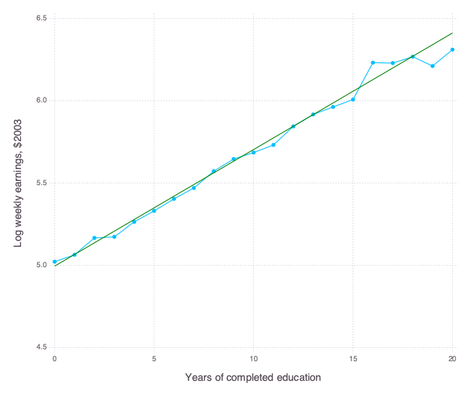
8 |
9 | ### Table 3-3-2
10 | Completed in [Stata](Table%203-3-2.do), [R](Table%203-3-2.r), [Python](Table%203-3-2.py) and [Julia](Table%203-3-2.jl)
11 |
12 | _Covariate means in the NSW and observational control samples_
13 |
14 | | |NSW Treat |NSW Control |Full CPS-1 |Full CPS-3 |P-score CPS-1 |P-score CPS-3 |
15 | |:------------------|:---------|:-----------|:----------|:----------|:-------------|:-------------|
16 | |Age |25.82 |25.05 |33.23 |28.03 |25.63 |25.97 |
17 | |Years of schooling |10.35 |10.09 |12.03 |10.24 |10.49 |10.42 |
18 | |Black |0.84 |0.83 |0.07 |0.2 |0.96 |0.52 |
19 | |Hispanic |0.06 |0.11 |0.07 |0.14 |0.03 |0.2 |
20 | |Dropout |0.71 |0.83 |0.3 |0.6 |0.6 |0.63 |
21 | |Married |0.19 |0.15 |0.71 |0.51 |0.26 |0.29 |
22 | |1974 earnings |2,096 |2,107 |14,017 |5,619 |2,821 |2,969 |
23 | |1975 earnings |1,532 |1,267 |13,651 |2,466 |1,950 |1,859 |
24 | |Number of Obs. |185 |260 |15,992 |429 |352 |157 |
25 |
26 | ### Figure 3-1-2
27 | Completed in [Stata](Figure%203-1-3.do), [R](Figure%203-1-3.r) and [Python](Figure%203-1-3.py)
28 |
29 | ```
30 | /* Old-fashioned standard errors */
31 |
32 | Source | SS df MS Number of obs = 329509
33 | -------------+------------------------------ F( 1,329507) =43782.56
34 | Model | 17808.83 1 17808.83 Prob > F = 0.0000
35 | Residual | 134029.045329507 .406756292 R-squared = 0.1173
36 | -------------+------------------------------ Adj R-squared = 0.1173
37 | Total | 151837.875329508 .460801788 Root MSE = .63777
38 |
39 | ------------------------------------------------------------------------------
40 | lwklywge | Coef. Std. Err. t P>|t| [95% Conf. Interval]
41 | -------------+----------------------------------------------------------------
42 | educ | .070851 .0003386 209.24 0.000 .0701874 .0715147
43 | _cons | 4.995182 .0044644 1118.88 0.000 4.986432 5.003932
44 | ------------------------------------------------------------------------------
45 |
46 | /* Robust standard errors */
47 |
48 | Linear regression Number of obs = 329509
49 | F( 1,329507) =34577.15
50 | Prob > F = 0.0000
51 | R-squared = 0.1173
52 | Root MSE = .63777
53 |
54 | ------------------------------------------------------------------------------
55 | | Robust
56 | lwklywge | Coef. Std. Err. t P>|t| [95% Conf. Interval]
57 | -------------+----------------------------------------------------------------
58 | educ | .070851 .000381 185.95 0.000 .0701042 .0715978
59 | _cons | 4.995182 .0050739 984.49 0.000 4.985238 5.005127
60 | ------------------------------------------------------------------------------
61 |
62 | /* Old-fashioned standard errors */
63 |
64 | Source | SS df MS Number of obs = 21
65 | -------------+------------------------------ F( 1, 19) = 485.23
66 | Model | 1.13497742 1 1.13497742 Prob > F = 0.0000
67 | Residual | .04444186 19 .002339045 R-squared = 0.9623
68 | -------------+------------------------------ Adj R-squared = 0.9603
69 | Total | 1.17941928 20 .058970964 Root MSE = .04836
70 |
71 | ------------------------------------------------------------------------------
72 | lwklywge | Coef. Std. Err. t P>|t| [95% Conf. Interval]
73 | -------------+----------------------------------------------------------------
74 | educ | .070851 .0032164 22.03 0.000 .064119 .0775831
75 | _cons | 4.995183 .0424075 117.79 0.000 4.906423 5.083943
76 | ------------------------------------------------------------------------------
77 |
78 | /* Robust standard errors */
79 |
80 | Linear regression Number of obs = 21
81 | F( 1, 19) = 231.81
82 | Prob > F = 0.0000
83 | R-squared = 0.9623
84 | Root MSE = .04836
85 |
86 | ------------------------------------------------------------------------------
87 | | Robust
88 | lwklywge | Coef. Std. Err. t P>|t| [95% Conf. Interval]
89 | -------------+----------------------------------------------------------------
90 | educ | .070851 .0046535 15.23 0.000 .0611112 .0805908
91 | _cons | 4.995183 .0479533 104.17 0.000 4.894815 5.09555
92 | ------------------------------------------------------------------------------
93 | ```
94 |
--------------------------------------------------------------------------------
3 |
4 | ## Synopsis
5 |
6 | A bold attempt to replicate the tables and figures from the book [_Mostly Harmless Econometrics_](http://www.mostlyharmlesseconometrics.com/) in the following languages:
7 | * Stata
8 | * R
9 | * Python
10 | * Julia
11 |
12 | Why undertake this madness? My primary motivation was to see if I could replace Stata with either R, Python, or Julia in my workflow, so I tried to replicate _Mostly Harmless Econometrics_ in each of these languages.
13 |
14 | ## Chapters
15 | 1. Questions about _Questions_
16 | 2. The Experimental Ideal
17 | 3. [Making Regression Make Sense](03%20Making%20Regression%20Make%20Sense/03%20Making%20Regression%20Make%20Sense.md)
18 | 4. [Instrumental Variables in Action](04%20Instrumental%20Variables%20in%20Action/04%20Instrumental%20Variables%20in%20Action.md)
19 | 5. [Parallel Worlds](05%20Fixed%20Effects%2C%20DD%20and%20Panel%20Data/05%20Fixed%20Effects%2C%20DD%20and%20Panel%20Data.md)
20 | 6. [Getting a Little Jumpy](06%20Getting%20a%20Little%20Jumpy/06%20Getting%20a%20Little%20Jumpy.md)
21 | 7. [Quantile Regression](07%20Quantile%20Regression/07%20Quantile%20Regression.md)
22 | 8. [Nonstandard Standard Error Issues](08%20Nonstandard%20Standard%20Error%20Issues/08%20Nonstanard%20Standard%20Error%20Issues.md)
23 |
24 | ## Getting started
25 | Check out [Getting Started](https://github.com/vikjam/mostly-harmless-replication/wiki/Getting-started) in the Wiki for tips on setting up your machine with each of these languages.
26 |
27 | ## Contributions
28 | Feel free to submit [pull requests](https://github.com/blog/1943-how-to-write-the-perfect-pull-request)!
29 |
30 |
--------------------------------------------------------------------------------
/03 Making Regression Make Sense/Figure 3-1-3.r:
--------------------------------------------------------------------------------
1 | # R code for Figure 3.1.3 #
2 | # Required packages #
3 | # - sandwhich: robust standard errors #
4 | # - lmtest: print table with robust standard errors #
5 | # - data.table: aggregate function #
6 | library(sandwich)
7 | library(lmtest)
8 |
9 | # Download data and unzip the data
10 | download.file('http://economics.mit.edu/files/397', 'asciiqob.zip')
11 | unzip('asciiqob.zip')
12 |
13 | # Read the data into a dataframe
14 | pums <- read.table('asciiqob.txt',
15 | header = FALSE,
16 | stringsAsFactors = FALSE)
17 | names(pums) <- c('lwklywge', 'educ', 'yob', 'qob', 'pob')
18 |
19 | # Panel A
20 | # Estimate OLS regression
21 | reg.model <- lm(lwklywge ~ educ, data = pums)
22 | # Robust standard errors
23 | robust.reg.vcov <- vcovHC(reg.model, "HC1")
24 | # Print results
25 | print(summary(reg.model))
26 | print(coeftest(reg.model, vcov = robust.reg.vcov))
27 |
28 | # Panel B
29 | # Figure out which observations appear in the regression
30 | sample <- !is.na(predict(reg.model, data = pums))
31 | pums.data.table <- data.table(pums[sample, ])
32 | # Aggregate
33 | educ.means <- pums.data.table[ , list(mean = mean(lwklywge),
34 | count = length(lwklywge)),
35 | by = educ]
36 | # Estimate weighted OLS regression
37 | wgt.reg.model <- lm(lwklywge ~ educ,
38 | weights = pums.data.table$count,
39 | data = pums.data.table)
40 | # Robust standard errors with weighted OLS regression
41 | wgt.robust.reg.vcov <- vcovHC(wgt.reg.model, "HC1")
42 | # Print results
43 | print(summary(wgt.reg.model))
44 | print(coeftest(wgt.reg.model, vcov = wgt.reg.vcov))
45 |
46 | # End of file
47 |
--------------------------------------------------------------------------------
/03 Making Regression Make Sense/Table 3-3-2.do:
--------------------------------------------------------------------------------
1 | clear all
2 | set more off
3 | eststo clear
4 | /* Required programs */
5 | /* - estout: output table */
6 |
7 | /* Stata code for Table 3.3.2 */
8 |
9 | * Store URL to MHE Data Archive in local
10 | local base_url = "https://economics.mit.edu/sites/default/files/inline-files"
11 |
12 | /* Store variable list in local */
13 | local summary_var "age ed black hisp nodeg married re74 re75"
14 | local pscore_var "age age2 ed black hisp married nodeg re74 re75"
15 |
16 | /* Columns 1 and 2 */
17 | use "`base_url'/nswre74.dta", clear
18 | eststo column_1, title("NSW Treat"): estpost summarize `summary_var' if treat == 1
19 | eststo column_2, title("NSW Control"): estpost summarize `summary_var' if treat == 0
20 |
21 | /* Column 3 */
22 | use "`base_url'/cps1re74.dta", clear
23 | eststo column_3, title("Full CPS-1"): estpost summarize `summary_var' if treat == 0
24 |
25 | /* Column 5 */
26 | probit treat `pscore_var'
27 | predict p_score, pr
28 | keep if p_score > 0.1 & p_score < 0.9
29 |
30 | eststo column_5, title("P-score CPS-1"): estpost summarize `summary_var' if treat == 0
31 |
32 | /* Column 4 */
33 | use "`base_url'/cps3re74.dta", clear
34 | eststo column_4, title("Full CPS-3"): estpost summarize `summary_var' if treat == 0
35 |
36 | /* Column 6 */
37 | probit treat `pscore_var'
38 | predict p_score, pr
39 | keep if p_score > 0.1 & p_score < 0.9
40 |
41 | eststo column_6, title("P-score CPS-3"): estpost summarize `summary_var' if treat == 0
42 |
43 | /* Label variables */
44 | label var age "Age"
45 | label var ed "Years of Schooling"
46 | label var black "Black"
47 | label var hisp "Hispanic"
48 | label var nodeg "Dropout"
49 | label var married "Married"
50 | label var re74 "1974 earnings"
51 | label var re75 "1975 earnings"
52 |
53 | /* Output Table */
54 | esttab column_1 column_2 column_3 column_4 column_5 column_6, ///
55 | label mtitle ///
56 | cells(mean(label(Mean) fmt(2 2 2 2 2 2 0 0)))
57 |
58 | /* End of script */
59 | exit
60 |
--------------------------------------------------------------------------------
/04 Instrumental Variables in Action/Figure 4-6-1.jl:
--------------------------------------------------------------------------------
1 | # Julia code for Table 4-6-1 #
2 | # Required packages #
3 | # - DataFrames: data manipulation / storage #
4 | # - Distributions: extended stats functions #
5 | # - FixedEffectModels: IV regression #
6 | using DataFrames
7 | using Distributions
8 | using FixedEffectModels
9 | using GLM
10 | using Gadfly
11 |
12 | # Number of simulations
13 | nsims = 1000
14 |
15 | # Set seed
16 | srand(113643)
17 |
18 | # Set parameters
19 | Sigma = [1.0 0.8;
20 | 0.8 1.0]
21 | N = 1000
22 |
23 | function irrelevantInstrMC()
24 | # Create Z, xi and eta
25 | Z = DataFrame(transpose(rand(MvNormal(eye(20)), N)))
26 | errors = DataFrame(transpose(rand(MvNormal(Sigma), N)))
27 |
28 | # Rename columns of Z and errors
29 | names!(Z, [Symbol("z$i") for i in 1:20])
30 | names!(errors, [:eta, :xi])
31 |
32 | # Create y and x
33 | df = hcat(Z, errors);
34 | df[:x] = 0.1 .* df[:z1] .+ df[:xi]
35 | df[:y] = df[:x] .+ df[:eta]
36 |
37 | # Run regressions
38 | ols = coef(lm(@formula(y ~ x), df))[2]
39 | tsls = coef(reg(df, @model(y ~ z1 + z2 + z3 + z4 + z5 + z6 + z7 + z8 + z9 + z10 +
40 | z11 + z12 + z13 + z14 + z15 + z16 + z17 + z18 + z19 + z20)))[2]
41 | return([ols tsls])
42 | end
43 |
44 | # Simulate IV regressions
45 | simulation_results = zeros(nsims, 2);
46 | for i = 1:nsims
47 | simulation_results[i, :] = irrelevantInstrMC()
48 | end
49 |
50 | # Create empirical CDFs from simulated results
51 | ols_ecdf = ecdf(simulation_results[:, 1])
52 | tsls_ecdf = ecdf(simulation_results[:, 2])
53 |
54 | # Plot the empirical CDFs of each estimator
55 | p = plot(layer(ols_ecdf, 0, 2.5, Theme(default_color = colorant"red")),
56 | layer(tsls_ecdf, 0, 2.5, Theme(line_style = :dot)),
57 | layer(xintercept = [0.5], Geom.vline,
58 | Theme(default_color = colorant"black", line_style = :dot)),
59 | layer(yintercept = [0.5], Geom.hline,
60 | Theme(default_color = colorant"black", line_style = :dot)),
61 | Guide.xlabel("Estimated β"),
62 | Guide.ylabel("Fn(Estimated β)"))
63 |
64 | # Export figure as .png
65 | draw(PNG("Figure 4-6-1-Julia.png", 7inch, 6inch), p)
66 |
67 | # End of script
68 |
--------------------------------------------------------------------------------
/06 Getting a Little Jumpy/Figure 6-1-1.py:
--------------------------------------------------------------------------------
1 | #!/usr/bin/env python
2 | """
3 | Create Figure 4-6-1 in MHE
4 | Tested on Python 3.4
5 | numpy: math and stat functions, array
6 | matplotlib: plot figures
7 | """
8 |
9 | import numpy as np
10 | import matplotlib.pyplot as plt
11 |
12 | # Set seed
13 | np.random.seed(10633)
14 |
15 | # Set number of simulations
16 | nobs = 100
17 |
18 | # Generate series
19 | x = np.random.uniform(0, 1, nobs)
20 | x = np.sort(x)
21 | y_linear = x + (x > 0.5) * 0.25 + np.random.normal(0, 0.1, nobs)
22 | y_nonlin = 0.5 * np.sin(6 * (x - 0.5)) + 0.5 + (x > 0.5) * 0.25 + np.random.normal(0, 0.1, nobs)
23 | y_mistake = 1 / (1 + np.exp(-25 * (x - 0.5))) + np.random.normal(0, 0.1, nobs)
24 |
25 | # Fit lines using user-created function
26 | def rdfit(x, y, cutoff, degree):
27 | coef_0 = np.polyfit(x[cutoff >= x], y[cutoff >= x], degree)
28 | fit_0 = np.polyval(coef_0, x[cutoff >= x])
29 |
30 | coef_1 = np.polyfit(x[x > cutoff], y[x > cutoff], degree)
31 | fit_1 = np.polyval(coef_1, x[x > cutoff])
32 |
33 | return coef_0, fit_0, coef_1, fit_1
34 |
35 | coef_y_linear_0 , fit_y_linear_0 , coef_y_linear_1 , fit_y_linear_1 = rdfit(x, y_linear, 0.5, 1)
36 | coef_y_nonlin_0 , fit_y_nonlin_0 , coef_y_nonlin_1 , fit_y_nonlin_1 = rdfit(x, y_nonlin, 0.5, 2)
37 | coef_y_mistake_0, fit_y_mistake_0, coef_y_mistake_1, fit_y_mistake_1 = rdfit(x, y_mistake, 0.5, 1)
38 |
39 | # Plot figures
40 | fig = plt.figure()
41 |
42 | ax1 = fig.add_subplot(311)
43 | ax1.scatter(x, y_linear, edgecolors = 'none')
44 | ax1.plot(x[0.5 >= x], fit_y_linear_0)
45 | ax1.plot(x[x > 0.5], fit_y_linear_1)
46 | ax1.axvline(0.5)
47 | ax1.set_title(r'A. Linear $E[Y_{0i} | X_i]$')
48 |
49 | ax2 = fig.add_subplot(312)
50 | ax2.scatter(x, y_nonlin, edgecolors = 'none')
51 | ax2.plot(x[0.5 >= x], fit_y_nonlin_0)
52 | ax2.plot(x[x > 0.5], fit_y_nonlin_1)
53 | ax2.axvline(0.5)
54 | ax2.set_title(r'B. Nonlinear $E[Y_{0i} | X_i]$')
55 |
56 | ax3 = fig.add_subplot(313)
57 | ax3.scatter(x, y_mistake, edgecolors = 'none')
58 | ax3.plot(x[0.5 >= x], fit_y_mistake_0)
59 | ax3.plot(x[x > 0.5], fit_y_mistake_1)
60 | ax3.plot(x, 1 / (1 + np.exp(-25 * (x - 0.5))), '--')
61 | ax3.axvline(0.5)
62 | ax3.set_title('C. Nonlinearity mistaken for discontinuity')
63 |
64 | plt.tight_layout()
65 | plt.savefig('Figure 6-1-1-Python.png', dpi = 300)
66 |
67 | # End of script
68 |
--------------------------------------------------------------------------------
/04 Instrumental Variables in Action/Table 4-1-1.r:
--------------------------------------------------------------------------------
1 | # R code for Table 4-1-1 #
2 | # Required packages #
3 | # - data.table: data management #
4 | # - sandwich: standard errors #
5 | # - AER: running IV regressions #
6 |
7 | library(data.table)
8 | library(sandwich)
9 | library(AER)
10 |
11 | # Download data and unzip the data
12 | download.file('http://economics.mit.edu/files/397', 'asciiqob.zip')
13 | unzip('asciiqob.zip')
14 |
15 | # Read the data into a data.table
16 | pums <- fread('asciiqob.txt',
17 | header = FALSE,
18 | stringsAsFactors = FALSE)
19 | names(pums) <- c('lwklywge', 'educ', 'yob', 'qob', 'pob')
20 |
21 | # Column 1: OLS
22 | col1 <- lm(lwklywge ~ educ, pums)
23 |
24 | # Column 2: OLS with YOB, POB dummies
25 | col2 <- lm(lwklywge ~ educ + factor(yob) + factor(pob), pums)
26 |
27 | # Create dummies for quarter of birth
28 | qobs <- unique(pums$qob)
29 | qobs.vars <- sapply(qobs, function(x) paste0('qob', x))
30 | pums[, (qobs.vars) := lapply(qobs, function(x) qob == x)]
31 |
32 | # Column 3: 2SLS with instrument QOB = 1
33 | col3 <- ivreg(lwklywge ~ educ, ~ qob1, pums)
34 |
35 | # Column 4: 2SLS with YOB, POB dummies and instrument QOB = 1
36 | col4 <- ivreg(lwklywge ~ factor(yob) + factor(pob) + educ,
37 | ~ factor(yob) + factor(pob) + qob1,
38 | pums)
39 |
40 | # Create dummy for quarter 1 or 2
41 | pums[, qob1or2 := qob == 1 | qob == 2]
42 |
43 | # Column 5: 2SLS with YOB, POB dummies and instrument (QOB = 1 | QOB = 2)
44 | col5 <- ivreg(lwklywge ~ factor(yob) + factor(pob) + educ,
45 | ~ factor(yob) + factor(pob) + qob1or2,
46 | pums)
47 |
48 | # Column 6: 2SLS with YOB, POB dummies and full QOB dummies
49 | col6 <- ivreg(lwklywge ~ factor(yob) + factor(pob) + educ,
50 | ~ factor(yob) + factor(pob) + factor(qob),
51 | pums)
52 |
53 | # Column 7: 2SLS with YOB, POB dummies and full QOB dummies interacted with YOB
54 | col7 <- ivreg(lwklywge ~ factor(yob) + factor(pob) + educ,
55 | ~ factor(pob) + factor(qob) * factor(yob),
56 | pums)
57 |
58 | # Column 8: 2SLS with age, YOB, POB dummies and with full QOB dummies interacted with YOB
59 | col8 <- ivreg(lwklywge ~ factor(yob) + factor(pob) + educ,
60 | ~ factor(pob) + factor(qob) * factor(yob),
61 | pums)
62 |
63 | # End of script
64 |
--------------------------------------------------------------------------------
/04 Instrumental Variables in Action/Figure 4-1-1.py:
--------------------------------------------------------------------------------
1 | #!/usr/bin/env python
2 | """
3 | Create Figure 4-6-1 in MHE
4 | Tested on Python 3.4
5 | """
6 |
7 | import zipfile
8 | import urllib.request
9 | import pandas as pd
10 | import statsmodels.api as sm
11 | import matplotlib.pyplot as plt
12 | from matplotlib.ticker import FormatStrFormatter
13 |
14 | # Download data and unzip the data
15 | urllib.request.urlretrieve('http://economics.mit.edu/files/397', 'asciiqob.zip')
16 | with zipfile.ZipFile('asciiqob.zip', "r") as z:
17 | z.extractall()
18 |
19 | # Read the data into a pandas dataframe
20 | pums = pd.read_csv('asciiqob.txt',
21 | header = None,
22 | delim_whitespace = True)
23 | pums.columns = ['lwklywge', 'educ', 'yob', 'qob', 'pob']
24 |
25 | # Calculate means by educ and lwklywge
26 | groupbybirth = pums.groupby(['yob', 'qob'])
27 | birth_means = groupbybirth['lwklywge', 'educ'].mean()
28 |
29 | # Create function to plot figures
30 | def plot_qob(yvar, ax, title, ylabel):
31 | values = yvar.values
32 | ax.plot(values, color = 'k')
33 |
34 | for i, y in enumerate(yvar):
35 | qob = yvar.index.get_level_values('qob')[i]
36 | ax.annotate(qob,
37 | (i, y),
38 | xytext = (-5, 5),
39 | textcoords = 'offset points')
40 | if qob == 1:
41 | ax.scatter(i, y, marker = 's', facecolors = 'none', edgecolors = 'k')
42 | else:
43 | ax.scatter(i, y, marker = 's', color = 'k')
44 |
45 | ax.set_xticks(range(0, len(yvar), 4))
46 | ax.set_xticklabels(yvar.index.get_level_values('yob')[1::4])
47 | ax.set_title(title)
48 | ax.set_ylabel(ylabel)
49 | ax.yaxis.set_major_formatter(FormatStrFormatter('%.2f'))
50 | ax.set_xlabel("Year of birth")
51 | ax.margins(0.1)
52 |
53 | fig, (ax1, ax2) = plt.subplots(2, sharex = True)
54 |
55 | plot_qob(yvar = birth_means['educ'],
56 | ax = ax1,
57 | title = 'A. Average education by quarter of birth (first stage)',
58 | ylabel = 'Years of education')
59 |
60 | plot_qob(yvar = birth_means['lwklywge'],
61 | ax = ax2,
62 | title = 'B. Average weekly wage by quarter of birth (reduced form)',
63 | ylabel = 'Log weekly earnings')
64 |
65 | fig.tight_layout()
66 | fig.savefig('Figure 4-1-1-Python.pdf', format = 'pdf')
67 |
68 | # End of file
69 |
--------------------------------------------------------------------------------
/06 Getting a Little Jumpy/Figure 6-1-1.r:
--------------------------------------------------------------------------------
1 | # R code for Figure 6-1-1 #
2 | # Required packages #
3 | # - ggplot2: making pretty graphs #
4 | # - gridExtra: combine graphs #
5 | library(ggplot2)
6 | library(gridExtra)
7 |
8 | # Generate series
9 | nobs = 100
10 | x <- runif(nobs)
11 | y.linear <- x + (x > 0.5) * 0.25 + rnorm(n = nobs, mean = 0, sd = 0.1)
12 | y.nonlin <- 0.5 * sin(6 * (x - 0.5)) + 0.5 + (x > 0.5) * 0.25 + rnorm(n = nobs, mean = 0, sd = 0.1)
13 | y.mistake <- 1 / (1 + exp(-25 * (x - 0.5))) + rnorm(n = nobs, mean = 0, sd = 0.1)
14 | rd.series <- data.frame(x, y.linear, y.nonlin, y.mistake)
15 |
16 | # Make graph with ggplot2
17 | g.data <- ggplot(rd.series, aes(x = x, group = x > 0.5))
18 |
19 | p.linear <- g.data + geom_point(aes(y = y.linear)) +
20 | stat_smooth(aes(y = y.linear),
21 | method = "lm",
22 | se = FALSE) +
23 | geom_vline(xintercept = 0.5) +
24 | ylab("Outcome") +
25 | ggtitle(bquote('A. Linear E[' * Y["0i"] * '|' * X[i] * ']'))
26 |
27 | p.nonlin <- g.data + geom_point(aes(y = y.nonlin)) +
28 | stat_smooth(aes(y = y.nonlin),
29 | method = "lm",
30 | formula = y ~ poly(x, 2),
31 | se = FALSE) +
32 | geom_vline(xintercept = 0.5) +
33 | ylab("Outcome") +
34 | ggtitle(bquote('B. Nonlinear E[' * Y["0i"] * '|' * X[i] * ']'))
35 |
36 | f.mistake <- function(x) {1 / (1 + exp(-25 * (x - 0.5)))}
37 | p.mistake <- g.data + geom_point(aes(y = y.mistake)) +
38 | stat_smooth(aes(y = y.mistake),
39 | method = "lm",
40 | se = FALSE) +
41 | stat_function(fun = f.mistake,
42 | linetype = "dashed") +
43 | geom_vline(xintercept = 0.5) +
44 | ylab("Outcome") +
45 | ggtitle('C. Nonlinearity mistaken for discontinuity')
46 |
47 | p.rd.examples <- arrangeGrob(p.linear, p.nonlin, p.mistake, ncol = 1)
48 |
49 | ggsave(p.rd.examples, file = "Figure 6-1-1-R.pdf", width = 5, height = 9)
50 |
51 | # End of script
52 |
--------------------------------------------------------------------------------
/04 Instrumental Variables in Action/Table 4-1-2.r:
--------------------------------------------------------------------------------
1 | # R code for Table 4-1-2 #
2 | # Required packages #
3 | # - data.table: data management #
4 | # - systemfit: SUR #
5 | library(data.table)
6 | library(systemfit)
7 |
8 | # Download data and unzip the data
9 | download.file('http://economics.mit.edu/files/397', 'asciiqob.zip')
10 | unzip('asciiqob.zip')
11 |
12 | # Read the data into a data.table
13 | pums <- fread('asciiqob.txt',
14 | header = FALSE,
15 | stringsAsFactors = FALSE)
16 | names(pums) <- c('lwklywge', 'educ', 'yob', 'qob', 'pob')
17 |
18 | # Create binary variable
19 | pums$z <- (pums$qob == 3 | pums$qob == 4) * 1
20 |
21 | # Compare means (and differences)
22 | ttest.lwklywge <- t.test(lwklywge ~ z, pums)
23 | ttest.educ <- t.test(educ ~ z, pums)
24 |
25 | # Compute Wald estimate
26 | sur <- systemfit(list(first = educ ~ z,
27 | second = lwklywge ~ z),
28 | data = pums,
29 | method = "SUR")
30 | wald <- deltaMethod(sur, "second_z / first_z")
31 |
32 | wald.estimate <- (mean(pums$lwklywge[pums$z == 1]) - mean(pums$lwklywge[pums$z == 0])) /
33 | (mean(pums$educ[pums$z == 1]) - mean(pums$educ[pums$z == 0]))
34 | wald.se <- wald.estimate^2 * ()
35 |
36 | # OLS estimate
37 | ols <- lm(lwklywge ~ educ, pums)
38 |
39 | # Construct table
40 | lwklywge.row <- c(ttest.lwklywge$estimate[1],
41 | ttest.lwklywge$estimate[2],
42 | ttest.lwklywge$estimate[2] - ttest.lwklywge$estimate[1])
43 | educ.row <- c(ttest.educ$estimate[1],
44 | ttest.educ$estimate[2],
45 | ttest.educ$estimate[2] - ttest.educ$estimate[1])
46 | wald.row.est <- c(NA, NA, wald$Estimate)
47 | wald.row.se <- c(NA, NA, wald$SE)
48 |
49 | ols.row.est <- c(NA, NA, summary(ols)$coef['educ' , 'Estimate'])
50 | ols.row.se <- c(NA, NA, summary(ols)$coef['educ' , 'Std. Error'])
51 |
52 | table <- rbind(lwklywge.row, educ.row,
53 | wald.row.est, wald.row.se,
54 | ols.row.est, ols.row.se)
55 | colnames(table) <- c("Born in the 1st or 2nd quarter of year",
56 | "Born in the 3rd or 4th quarter of year",
57 | "Difference")
58 | rownames(table) <- c("ln(weekly wage)",
59 | "Years of education",
60 | "Wald estimate",
61 | "Wald std error",
62 | "OLS estimate",
63 | "OLS std error")
64 |
65 | # End of script
66 |
--------------------------------------------------------------------------------
/08 Nonstandard Standard Error Issues/08 Nonstanard Standard Error Issues.md:
--------------------------------------------------------------------------------
1 | # 08 Nonstandard Standard Error Issues
2 | ## 8.1 The Bias of Robust Standard Errors
3 |
4 | ### Table 8.1.1
5 | Completed in [Stata](Table%208-1-1.do), [R](Table%208-1-1.r), [Python](Table%208-1-1.py) and [Julia](Table%208-1-1.jl)
6 |
7 | _Panel A: Lots of Heteroskedasticity_
8 |
9 | |Estimate | Mean| Std| Normal| t|
10 | |:----------------------|------:|-----:|------:|-----:|
11 | |Beta_1 | -0.006| 0.581| NA| NA|
12 | |Conventional | 0.331| 0.052| 0.269| 0.249|
13 | |HC0 | 0.433| 0.210| 0.227| 0.212|
14 | |HC1 | 0.448| 0.218| 0.216| 0.201|
15 | |HC2 | 0.525| 0.260| 0.171| 0.159|
16 | |HC3 | 0.638| 0.321| 0.124| 0.114|
17 | |max(Conventional, HC0) | 0.461| 0.182| 0.174| 0.159|
18 | |max(Conventional, HC1) | 0.474| 0.191| 0.167| 0.152|
19 | |max(Conventional, HC2) | 0.543| 0.239| 0.136| 0.123|
20 | |max(Conventional, HC3) | 0.650| 0.305| 0.101| 0.091|
21 |
22 | _Panel B: Little Heteroskedasticity_
23 |
24 | |Estimate | Mean| Std| Normal| t|
25 | |:----------------------|------:|-----:|------:|-----:|
26 | |Beta_1 | -0.006| 0.595| NA| NA|
27 | |Conventional | 0.519| 0.070| 0.097| 0.084|
28 | |HC0 | 0.456| 0.200| 0.204| 0.188|
29 | |HC1 | 0.472| 0.207| 0.191| 0.175|
30 | |HC2 | 0.546| 0.251| 0.153| 0.140|
31 | |HC3 | 0.656| 0.312| 0.112| 0.102|
32 | |max(Conventional, HC0) | 0.569| 0.130| 0.081| 0.070|
33 | |max(Conventional, HC1) | 0.577| 0.139| 0.079| 0.067|
34 | |max(Conventional, HC2) | 0.625| 0.187| 0.068| 0.058|
35 | |max(Conventional, HC3) | 0.712| 0.260| 0.054| 0.045|
36 |
37 | _Panel C: No Heteroskedasticity_
38 |
39 | |Estimate | Mean| Std| Normal| t|
40 | |:----------------------|------:|-----:|------:|-----:|
41 | |Beta_1 | -0.006| 0.604| NA| NA|
42 | |Conventional | 0.603| 0.081| 0.059| 0.049|
43 | |HC0 | 0.469| 0.196| 0.193| 0.177|
44 | |HC1 | 0.485| 0.203| 0.180| 0.165|
45 | |HC2 | 0.557| 0.246| 0.145| 0.131|
46 | |HC3 | 0.667| 0.308| 0.106| 0.097|
47 | |max(Conventional, HC0) | 0.633| 0.116| 0.052| 0.043|
48 | |max(Conventional, HC1) | 0.639| 0.123| 0.051| 0.042|
49 | |max(Conventional, HC2) | 0.678| 0.166| 0.045| 0.036|
50 | |max(Conventional, HC3) | 0.752| 0.237| 0.036| 0.030|
51 |
--------------------------------------------------------------------------------
/04 Instrumental Variables in Action/Figure 4-1-1.r:
--------------------------------------------------------------------------------
1 | # R code for Figure 4-1-1 #
2 | # Required packages #
3 | # - dplyr: easy data manipulation #
4 | # - lubridate: data management #
5 | # - ggplot2: making pretty graphs #
6 | # - gridExtra: combine graphs #
7 | library(lubridate)
8 | library(dplyr)
9 | library(ggplot2)
10 | library(gridExtra)
11 |
12 | # Download data and unzip the data
13 | download.file('http://economics.mit.edu/files/397', 'asciiqob.zip')
14 | unzip('asciiqob.zip')
15 |
16 | # Read the data into a dataframe
17 | pums <- read.table('asciiqob.txt',
18 | header = FALSE,
19 | stringsAsFactors = FALSE)
20 | names(pums) <- c('lwklywge', 'educ', 'yob', 'qob', 'pob')
21 |
22 | # Collapse for means
23 | pums.qob.means <- pums %>% group_by(yob, qob) %>% summarise_each(funs(mean))
24 |
25 | # Add dates
26 | pums.qob.means$yqob <- ymd(paste0("19",
27 | pums.qob.means$yob,
28 | pums.qob.means$qob * 3),
29 | truncated = 2)
30 |
31 | # Function for plotting data
32 | plot.qob <- function(ggplot.obj, ggtitle, ylab) {
33 | gg.colours <- c("firebrick", rep("black", 3), "white")
34 | ggplot.obj + geom_line() +
35 | geom_point(aes(colour = factor(qob)),
36 | size = 5) +
37 | geom_text(aes(label = qob, colour = "white"),
38 | size = 3,
39 | hjust = 0.5, vjust = 0.5,
40 | show_guide = FALSE) +
41 | scale_colour_manual(values = gg.colours, guide = FALSE) +
42 | ggtitle(ggtitle) +
43 | xlab("Year of birth") +
44 | ylab(ylab) +
45 | theme_set(theme_gray(base_size = 10))
46 | }
47 |
48 | # Plot
49 | p.educ <- plot.qob(ggplot(pums.qob.means, aes(x = yqob, y = educ)),
50 | "A. Average education by quarter of birth (first stage)",
51 | "Years of education")
52 | p.lwklywge <- plot.qob(ggplot(pums.qob.means, aes(x = yqob, y = lwklywge)),
53 | "B. Average weekly wage by quarter of birth (reduced form)",
54 | "Log weekly earnings")
55 |
56 | p.ivgraph <- arrangeGrob(p.educ, p.lwklywge)
57 |
58 | ggsave(p.ivgraph, file = "Figure 4-1-1-R.png", height = 12, width = 8, dpi = 300)
59 |
60 | # End of script
61 |
--------------------------------------------------------------------------------
/06 Getting a Little Jumpy/Figure 6-2-1.r:
--------------------------------------------------------------------------------
1 | # R code for Figure 6-2-1 #
2 | # Required packages #
3 | # - haven: read Stata .dta files #
4 | # - ggplot2: making pretty graphs #
5 | # - gridExtra: combine graphs #
6 | library(haven)
7 | library(ggplot2)
8 | library(gridExtra)
9 |
10 | # Download the data
11 | download.file("http://economics.mit.edu/files/1359", "final4.dta")
12 | download.file("http://economics.mit.edu/files/1358", "final5.dta")
13 |
14 | # Load the data
15 | grade4 <- read_dta("final4.dta")
16 | grade5 <- read_dta("final5.dta")
17 |
18 | # Restrict sample
19 | grade4 <- grade4[which(grade4$classize & grade4$classize < 45 & grade4$c_size > 5), ]
20 | grade5 <- grade5[which(grade5$classize & grade5$classize < 45 & grade5$c_size > 5), ]
21 |
22 | # Find means class size by grade size
23 | grade4cmeans <- aggregate(grade4$classize,
24 | by = list(grade4$c_size),
25 | FUN = mean,
26 | na.rm = TRUE)
27 | grade5cmeans <- aggregate(grade5$classize,
28 | by = list(grade5$c_size),
29 | FUN = mean,
30 | na.rm = TRUE)
31 |
32 | # Rename aggregaed columns
33 | colnames(grade4cmeans) <- c("c_size", "classize.mean")
34 | colnames(grade5cmeans) <- c("c_size", "classize.mean")
35 |
36 | # Create function for Maimonides Rule
37 | maimonides.rule <- function(x) {x / (floor((x - 1)/40) + 1)}
38 |
39 | # Plot each grade
40 | g4 <- ggplot(data = grade4cmeans, aes(x = c_size))
41 | p4 <- g4 + geom_line(aes(y = classize.mean)) +
42 | stat_function(fun = maimonides.rule,
43 | linetype = "dashed") +
44 | expand_limits(y = 0) +
45 | scale_x_continuous(breaks = seq(0, 220, 20)) +
46 | ylab("Class size") +
47 | xlab("Enrollment count") +
48 | ggtitle("B. Fourth grade")
49 |
50 | g5 <- ggplot(data = grade5cmeans, aes(x = c_size))
51 | p5 <- g5 + geom_line(aes(y = classize.mean)) +
52 | stat_function(fun = maimonides.rule,
53 | linetype = "dashed") +
54 | expand_limits(y = 0) +
55 | scale_x_continuous(breaks = seq(0, 220, 20)) +
56 | ylab("Class size") +
57 | xlab("Enrollment count") +
58 | ggtitle("A. Fifth grade")
59 |
60 | first.stage <- arrangeGrob(p5, p4, ncol = 1)
61 | ggsave(first.stage, file = "Figure 6-2-1-R.png", height = 8, width = 5, dpi = 300)
62 |
63 | # End of script
64 |
--------------------------------------------------------------------------------
/07 Quantile Regression/Table 7-1-1.r:
--------------------------------------------------------------------------------
1 | # R code for Table 7.1.1 #
2 | # Required packages #
3 | # - haven: read in .dta files #
4 | # - quantreg: quantile regressions #
5 | # - knitr: markdown tables #
6 | library(haven)
7 | library(quantreg)
8 | library(knitr)
9 |
10 | # Download data and unzip the data
11 | download.file('http://economics.mit.edu/files/384', 'angcherfer06.zip')
12 | unzip('angcherfer06.zip')
13 |
14 | # Create a function to run the quantile/OLS regressions so we can use a loop
15 | quant.mincer <- function(tau, data) {
16 | r <- rq(logwk ~ educ + black + exper + exper2,
17 | weights = perwt,
18 | data = data,
19 | tau = tau)
20 | return(rbind(summary(r)$coefficients["educ", "Value"],
21 | summary(r)$coefficients["educ", "Std. Error"]))
22 | }
23 |
24 | # Create function for producing the results
25 | calculate.qr <- function(year) {
26 |
27 | # Create file path
28 | dta.path <- paste('Data/census', year, '.dta', sep = "")
29 |
30 | # Load year into the census
31 | df <- read_dta(dta.path)
32 |
33 | # Run quantile regressions
34 | taus <- c(0.1, 0.25, 0.5, 0.75, 0.9)
35 | qr <- sapply(taus, quant.mincer, data = df)
36 |
37 | # Run OLS regressions and get RMSE
38 | ols <- lm(logwk ~ educ + black + exper + exper2,
39 | weights = perwt,
40 | data = df)
41 | coef.se <- rbind(summary(ols)$coefficients["educ", "Estimate"],
42 | summary(ols)$coefficients["educ", "Std. Error"])
43 | rmse <- sqrt(sum(summary(ols)$residuals^2) / ols$df.residual)
44 |
45 | # Summary statistics
46 | obs <- length(na.omit(df$educ))
47 | mean <- mean(df$logwk, na.rm = TRUE)
48 | sd <- sd(df$logwk, na.rm = TRUE)
49 |
50 | return(cbind(rbind(obs, NA),
51 | rbind(mean, NA),
52 | rbind(sd, NA),
53 | qr,
54 | coef.se,
55 | rbind(rmse, NA)))
56 |
57 | }
58 |
59 | # Generate results
60 | results <- rbind(calculate.qr("80"),
61 | calculate.qr("90"),
62 | calculate.qr("00"))
63 |
64 | # Name rows and columns
65 | row.names(results) <- c("1980", "", "1990", "", "2000", "")
66 | colnames(results) <- c("Obs", "Mean", "Std Dev",
67 | "0.1", "0.25", "0.5", "0.75", "0.9",
68 | "OLS", "RMSE")
69 |
70 | # Format decimals
71 | results <- round(results, 3)
72 | results[ , c(2, 10)] <- round(results[ , c(2, 10)], 2)
73 | results[ , 1] <- formatC(results[ , 1], format = "d", big.mark = ",")
74 |
75 | # Export table
76 | print(kable(results))
77 |
78 | # End of file
79 |
--------------------------------------------------------------------------------
/03 Making Regression Make Sense/Table 3-3-2.py:
--------------------------------------------------------------------------------
1 | #!/usr/bin/env python
2 | """
3 | Tested on Python 3.11.13
4 | """
5 |
6 | import urllib.request
7 | import pandas as pd
8 | import statsmodels.api as sm
9 | import numpy as np
10 | import patsy
11 | from tabulate import tabulate
12 |
13 | # Read the Stata files into Python directly from website
14 | base_url = 'https://economics.mit.edu/sites/default/files/inline-files'
15 | nswre74 = pd.read_stata(f"{base_url}/nswre74.dta")
16 | cps1re74 = pd.read_stata(f"{base_url}/cps1re74.dta")
17 | cps3re74 = pd.read_stata(f"{base_url}/cps3re74.dta")
18 |
19 | # Store list of variables for summary
20 | summary_vars = ['age', 'ed', 'black', 'hisp', 'nodeg', 'married', 're74', 're75']
21 |
22 | # Calculate propensity scores
23 | # Create formula for probit
24 | f = 'treat ~ ' + ' + '.join(['age', 'age2', 'ed', 'black', 'hisp', \
25 | 'nodeg', 'married', 're74', 're75'])
26 |
27 | # Run probit with CPS-1
28 | y, X = patsy.dmatrices(f, cps1re74, return_type = 'dataframe')
29 | model = sm.Probit(y, X).fit()
30 | cps1re74['pscore'] = model.predict(X)
31 |
32 | # Run probit with CPS-3
33 | y, X = patsy.dmatrices(f, cps3re74, return_type = 'dataframe')
34 | model = sm.Probit(y, X).fit()
35 | cps3re74['pscore'] = model.predict(X)
36 |
37 | # Create function to summarize data
38 | def summarize(dataset, conditions):
39 | stats = dataset[summary_vars][conditions].mean()
40 | stats['count'] = sum(conditions)
41 | return stats
42 |
43 | # Summarize data
44 | nswre74_treat_stats = summarize(nswre74, nswre74.treat == 1)
45 | nswre74_control_stats = summarize(nswre74, nswre74.treat == 0)
46 | cps1re74_control_stats = summarize(cps1re74, cps1re74.treat == 0)
47 | cps3re74_control_stats = summarize(cps3re74, cps3re74.treat == 0)
48 | cps1re74_ptrim_stats = summarize(cps1re74, (cps1re74.treat == 0) & \
49 | (cps1re74.pscore > 0.1) & \
50 | (cps1re74.pscore < 0.9))
51 | cps3re74_ptrim_stats = summarize(cps3re74, (cps3re74.treat == 0) & \
52 | (cps3re74.pscore > 0.1) & \
53 | (cps3re74.pscore < 0.9))
54 |
55 | # Combine summary stats, add header and print to markdown
56 | frames = [nswre74_treat_stats,
57 | nswre74_control_stats,
58 | cps1re74_control_stats,
59 | cps3re74_control_stats,
60 | cps1re74_ptrim_stats,
61 | cps3re74_ptrim_stats]
62 |
63 | summary_stats = pd.concat(frames, axis = 1)
64 | header = ["NSW Treat", "NSW Control", \
65 | "Full CPS-1", "Full CPS-3", \
66 | "P-score CPS-1", "P-score CPS-3"]
67 |
68 | print(tabulate(summary_stats, header, tablefmt = "pipe"))
69 |
70 | # End of script
71 |
--------------------------------------------------------------------------------
/04 Instrumental Variables in Action/Figure 4-6-1.do:
--------------------------------------------------------------------------------
1 | clear all
2 | set more off
3 | capture log close _all
4 | capture version 13.1 // Note this script has only been tested in Stata 13.1
5 |
6 | /* Stata code for Figure 4.6.1 */
7 |
8 | /* Log output*/
9 | log using "Figure 4-6-1-Stata.txt", name(figure040601) text replace
10 |
11 | /* Set random seed for replication */
12 | set seed 42
13 |
14 | /* Define program for use with -simulate- command */
15 | capture program drop weakinstr
16 | program define weakinstr, rclass
17 | version 13.1
18 |
19 | /* Draw from random normal with correlation of 0.8 and variance of 1 */
20 | matrix C = (1, 0.8 \ 0.8, 1)
21 | quietly drawnorm eta xi, n(1000) corr(C) clear
22 |
23 | /* Create a random instruments */
24 | forvalues i = 1/20 {
25 | quietly gen z`i' = rnormal()
26 | }
27 |
28 | /* Endogenous x only based on z1 while z2-z20 irrelevant */
29 | quietly gen x = 0.1*z1 + xi
30 | quietly gen y = x + eta
31 |
32 | /* OLS */
33 | quietly: regress y x
34 | matrix OLS = e(b)
35 |
36 | /* 2SLS */
37 | quietly: ivregress 2sls y (x = z*)
38 | matrix TSLS = e(b)
39 |
40 | /* LIML */
41 | quietly: ivregress liml y (x = z*)
42 | matrix LIML = e(b)
43 |
44 | /* Return results from program */
45 | return scalar ols = OLS[1, 1]
46 | return scalar tsls = TSLS[1, 1]
47 | return scalar liml = LIML[1, 1]
48 |
49 | end
50 |
51 | /* Run simulation */
52 | simulate coefols = r(ols) coeftsls = r(tsls) coefliml = r(liml), reps(10000): weakinstr
53 |
54 | /* Create empirical CDFs */
55 | cumul coefols, gen(cols)
56 | cumul coeftsls, gen(ctsls)
57 | cumul coefliml, gen(climl)
58 | stack cols coefols ctsls coeftsls climl coefliml, into(c coef) wide clear
59 | label var coef "beta"
60 | label var cols "OLS"
61 | label var ctsls "2SLS"
62 | label var climl "LIML"
63 |
64 | /* Graph results */
65 | graph set window fontface "Palatino"
66 | line cols ctsls climl coef if inrange(coef, 0, 2.5), ///
67 | sort ///
68 | lpattern(solid dash longdash_dot) ///
69 | lwidth(medthick medthick medthick) ///
70 | lcolor("228 26 28" "55 126 184" "77 175 74") ///
71 | scheme(s1color) ///
72 | legend(rows(1) region(lwidth(none))) ///
73 | xline(1, lcolor("189 189 189") lpattern(shortdash) lwidth(medthick)) ///
74 | yline(0.5, lcolor("189 189 189") lpattern(shortdash) lwidth(medthick)) ///
75 | xtitle("estimated {&beta}") ///
76 | ytitle("F{subscript:n}")
77 | graph export "Figure 4-6-1-Stata.eps", replace
78 |
79 | log close figure040601
80 | /* End of script */
81 |
--------------------------------------------------------------------------------
/04 Instrumental Variables in Action/Figure 4-6-1.r:
--------------------------------------------------------------------------------
1 | # R code for Figure 4.6.1 #
2 | # Required packages #
3 | # - MASS: multivariate normal draws #
4 | # - ivmodel: IV regressions #
5 | # - parallel: Parallel process simulation #
6 | # - ggplot2: making pretty graphs #
7 | # - RColorBrewer: pleasing color schemes #
8 | # - reshape: manipulate data #
9 | library(MASS)
10 | library(ivmodel)
11 | library(parallel)
12 | library(ggplot2)
13 | library(RColorBrewer)
14 | library(reshape)
15 |
16 | nsims = 100000
17 | set.seed(1984, "L'Ecuyer")
18 |
19 | irrelevantInstrMC <- function(...) {
20 | # Store coefficients
21 | COEFS <- rep(NA, 3)
22 | names(COEFS) <- c("ols", "tsls", "liml")
23 |
24 | # Set parameters
25 | Sigma = matrix(c(1, 0.8, 0.8, 1), 2, 2)
26 | errors = mvrnorm(n = 1000, rep(0, 2), Sigma)
27 | eta = errors[ , 1]
28 | xi = errors[ , 2]
29 |
30 | # Create Z, x, y
31 | Z = sapply(1:20, function(x) rnorm(1000))
32 | x = 0.1 * Z[ , 1] + xi
33 | y = x + eta
34 |
35 | # OLS
36 | OLS <- lm(y ~ x)
37 | COEFS["ols"] <- summary(OLS)$coefficients[2, 1]
38 |
39 | # Run IV regressions
40 | ivregressions <- ivmodel(Y = y, D = x, Z = Z)
41 | COEFS["tsls"] <- coef.ivmodel(ivregressions)["TSLS", "Estimate"]
42 | COEFS["liml"] <- coef.ivmodel(ivregressions)["LIML", "Estimate"]
43 |
44 | # Return results
45 | return(COEFS)
46 | }
47 |
48 | # Run simulations
49 | SIMBETAS <- data.frame(t(simplify2array(mclapply(1:nsims, irrelevantInstrMC))))
50 |
51 | df <- melt(SIMBETAS[ , 1:3])
52 | names(df) <- c("Estimator", "beta")
53 | df$Estimator <- factor(df$Estimator,
54 | levels = c("ols", "tsls", "liml"),
55 | labels = c("OLS", "2SLS", "LIML"))
56 |
57 | g <- ggplot(df, aes(x = beta, colour = Estimator, linetype = Estimator)) +
58 | stat_ecdf(geom = "step") +
59 | xlab(expression(widehat(beta))) + ylab(expression(F[n](widehat(beta)))) +
60 | xlim(0, 2.5) +
61 | scale_linetype_manual(values = c("solid", "longdash", "twodash")) +
62 | scale_color_manual(values = brewer.pal(3, "Set1"),
63 | labels = c("OLS", "2SLS", "LIML")) +
64 | geom_vline(xintercept = 1.0, linetype = "longdash") +
65 | geom_hline(yintercept = 0.5, linetype = "longdash") +
66 | theme(axis.title.y = element_text(angle=0)) +
67 | theme_set(theme_gray(base_size = 24))
68 | ggsave(file = "Figure 4-6-1-R.png", height = 8, width = 12, dpi = 300)
69 |
70 | write.csv(df, "Figure 4-6-1.csv")
71 | # End of script
72 |
--------------------------------------------------------------------------------
/04 Instrumental Variables in Action/Figure 4-1-1.do:
--------------------------------------------------------------------------------
1 | clear all
2 | set more off
3 | /* Stata code for Figure 4-1-1 */
4 |
5 | /* Download data */
6 | shell curl -o asciiqob.zip http://economics.mit.edu/files/397
7 | unzipfile asciiqob.zip, replace
8 |
9 | /* Import data */
10 | infile lwklywge educ yob qob pob using asciiqob.txt, clear
11 |
12 | /* Use Stata date formats */
13 | gen yqob = yq(1900 + yob, qob)
14 | format yqob %tq
15 |
16 | /* Collapse by quarter of birth */
17 | collapse (mean) educ (mean) lwklywge (mean) qob, by(yqob)
18 |
19 | /* Plot data */
20 | graph twoway (line educ yqob, lcolor(black)) ///
21 | (scatter educ yqob if qob == 1, ///
22 | mlabel(qob) msize(small) msymbol(S) mcolor(black)) ///
23 | (scatter educ yqob if qob != 1, ///
24 | mlabel(qob) msize(small) msymbol(Sh) mcolor(black)), ///
25 | xlabel(, format(%tqY)) ///
26 | title("A. Average education by quarter of birth (first stage)") ///
27 | ytitle("Years of education") ///
28 | xtitle("Year of birth") ///
29 | legend(off) ///
30 | name(educ) ///
31 | scheme(s1mono)
32 |
33 | graph twoway (line lwklywge yqob, lcolor(black)) ///
34 | (scatter lwklywge yqob if qob == 1, ///
35 | mlabel(qob) msize(small) msymbol(S) mcolor(black)) ///
36 | (scatter lwklywge yqob if qob != 1, ///
37 | mlabel(qob) msize(small) msymbol(Sh) mcolor(black)), ///
38 | xlabel(, format(%tqY)) ///
39 | title("B. Average weekly wage by quarter of birth (reduced form)") ///
40 | ytitle("Log weekly earnings") ///
41 | xtitle("Year of birth") ///
42 | legend(off) ///
43 | name(lwklywge) ///
44 | scheme(s1mono)
45 |
46 | /* Compare graphs */
47 | graph combine educ lwklywge, ///
48 | col(1) ///
49 | xsize(4) ysize(6) ///
50 | graphregion(margin(zero)) ///
51 | scheme(s1mono)
52 |
53 | graph export "Figure 4-1-1-Stata.pdf", replace
54 |
55 | /* End of file */
56 |
--------------------------------------------------------------------------------
/06 Getting a Little Jumpy/Figure 6-2-1.do:
--------------------------------------------------------------------------------
1 | clear all
2 | set more off
3 |
4 | /* Download data */
5 | shell curl -o final4.dta http://economics.mit.edu/files/1359
6 | shell curl -o final5.dta http://economics.mit.edu/files/1358
7 |
8 | /*---------*/
9 | /* Grade 4 */
10 | /*---------*/
11 | /* Import data */
12 | use "final4.dta", clear
13 |
14 | /* Restrict sample */
15 | keep if 1 < classize & classize < 45 & c_size > 5
16 |
17 | /* Find means class size by grade size */
18 | collapse classize, by(c_size)
19 |
20 | /* Plot the actual and predicted class size based on grade size */
21 | graph twoway (line classize c_size, lcolor(black)) ///
22 | (function y = x / (floor((x - 1)/40) + 1), ///
23 | range(1 220) lpattern(dash) lcolor(black)), ///
24 | xlabel(20(20)220) ///
25 | title("B. Fourth grade") ///
26 | ytitle("Class size") ///
27 | xtitle("Enrollment count") ///
28 | legend(label(1 "Actual class size") label(2 "Maimonides Rule")) ///
29 | scheme(s1mono) ///
30 | saving(fourthgrade.gph, replace)
31 |
32 | /*---------*/
33 | /* Grade 5 */
34 | /*---------*/
35 | /* Import data */
36 | use "final5.dta", clear
37 |
38 | /* Restrict sample */
39 | keep if 1 < classize & classize < 45 & c_size > 5
40 |
41 | /* Find means class size by grade size */
42 | collapse classize, by(c_size)
43 |
44 | /* Plot the actual and predicted class size based on grade size */
45 | graph twoway (line classize c_size, lcolor(black)) ///
46 | (function y = x / (floor((x - 1)/40) + 1), ///
47 | range(1 220) lpattern(dash) lcolor(black)), ///
48 | xlabel(20(20)220) ///
49 | title("A. Fifth grade") ///
50 | ytitle("Class size") ///
51 | xtitle("Enrollment count") ///
52 | legend(label(1 "Actual class size") label(2 "Maimonides Rule")) ///
53 | scheme(s1mono) ///
54 | saving(fifthgrade.gph, replace)
55 |
56 | /* Combine graphs */
57 | graph combine fifthgrade.gph fourthgrade.gph, ///
58 | col(1) ///
59 | xsize(4) ysize(6) ///
60 | graphregion(margin(zero)) ///
61 | scheme(s1mono)
62 | graph export "Figure 6-2-1-Stata.png", replace
63 |
64 | /* End of file */
65 | exit
66 |
--------------------------------------------------------------------------------
/03 Making Regression Make Sense/Table 3-3-2.jl:
--------------------------------------------------------------------------------
1 | # Load packages
2 | using DataFrames
3 | using FileIO, StatFiles
4 | using Statistics
5 | using GLM
6 |
7 | # Download the data from the MHE Data Archive
8 | base_url = "https://economics.mit.edu/sites/default/files/inline-files"
9 | download("$(base_url)/nswre74.dta", "nswre74.dta")
10 | download("$(base_url)/cps1re74.dta", "cps1re74.dta")
11 | download("$(base_url)/cps3re74.dta", "cps3re74.dta")
12 |
13 | # Read the Stata files into Julia
14 | nswre74 = DataFrame(load("nswre74.dta"))
15 | cps1re74 = DataFrame(load("cps1re74.dta"))
16 | cps3re74 = DataFrame(load("cps3re74.dta"))
17 |
18 | summary_vars = [:age, :ed, :black, :hisp, :nodeg, :married, :re74, :re75]
19 | nswre74_stat = combine(nswre74, summary_vars .=> mean)
20 |
21 | # Calculate propensity scores
22 | probit = glm(@formula(treat ~ age + age2 + ed + black + hisp +
23 | nodeg + married + re74 + re75),
24 | cps1re74,
25 | Binomial(),
26 | ProbitLink())
27 | cps1re74.pscore = predict(probit)
28 |
29 | probit = glm(@formula(treat ~ age + age2 + ed + black + hisp +
30 | nodeg + married + re74 + re75),
31 | cps3re74,
32 | Binomial(),
33 | ProbitLink())
34 | cps3re74.pscore = predict(probit)
35 |
36 | # Create function to summarize data
37 | function summarize(data, condition)
38 | stats = combine(data[condition, :], summary_vars .=> mean)
39 | stats.count = [size(data[condition, summary_vars])[1]]
40 | return(stats)
41 | end
42 |
43 | # Summarize data
44 | nswre74_treat_stats = summarize(nswre74, nswre74.treat .== 1)
45 | nswre74_control_stats = summarize(nswre74, nswre74.treat .== 0)
46 | cps1re74_control_stats = summarize(cps1re74, cps1re74.treat .== 0)
47 | cps3re74_control_stats = summarize(cps3re74, cps3re74.treat .== 0)
48 | cps1re74_ptrim_stats = summarize(cps1re74, broadcast(&, cps1re74.treat .== 0,
49 | cps1re74.pscore .> 0.1,
50 | cps1re74.pscore .< 0.9))
51 | cps3re74_ptrim_stats = summarize(cps3re74, broadcast(&, cps3re74.treat .== 0,
52 | cps3re74.pscore .> 0.1,
53 | cps3re74.pscore .< 0.9))
54 |
55 | # Combine summary stats, add header and print to markdown
56 | table = vcat(nswre74_treat_stats,
57 | nswre74_control_stats,
58 | cps1re74_control_stats,
59 | cps3re74_control_stats,
60 | cps1re74_ptrim_stats,
61 | cps3re74_ptrim_stats)
62 | table.id = 1:size(table, 1)
63 | table = stack(table, [:age_mean, :ed_mean, :black_mean, :hisp_mean,
64 | :nodeg_mean, :married_mean, :re74_mean, :re75_mean, :count])
65 | table = unstack(table, :variable, :id, :value)
66 |
67 | rename!(table, [:Variable, :NSWTreat, :NSWControl,
68 | :FullCPS1, :FullCPS3, :PscoreCPS1, :PscoreCPS3])
69 |
70 | println(table)
71 |
72 | # End of script
73 |
--------------------------------------------------------------------------------
/06 Getting a Little Jumpy/Figure 6-1-1.jl:
--------------------------------------------------------------------------------
1 | # Load packages
2 | using Random
3 | using DataFrames
4 | using Gadfly
5 | using Cairo
6 | using Fontconfig
7 | using Distributions
8 | using CurveFit
9 | using Colors
10 |
11 | # Set seed
12 | Random.seed!(08421);
13 |
14 | # Set number of simulations
15 | nsims = 100
16 |
17 | # Set distributions for random draws
18 | uniform = Uniform(0, 1)
19 | normal = Normal(0, 0.1)
20 |
21 | # Generate series
22 | x = rand(uniform, nsims)
23 | y_linear = x .+ (x .> 0.5) .* 0.25 .+ rand(normal, nsims)
24 | y_nonlin = 0.5 .* sin.(6 .* (x .- 0.5)) .+ 0.5 .+ (x .> 0.5) .* 0.25 .+ rand(normal, nsims)
25 | y_mistake = 1 ./ (1 .+ exp.(-25 .* (x .- 0.5))) .+ rand(normal, nsims)
26 |
27 | # Fit lines using user-created function
28 | function rdfit(xvar, yvar, cutoff, degree)
29 | coef_0 = curve_fit(Poly, xvar[cutoff .>= x], yvar[cutoff .>= x], degree)
30 | fit_0 = coef_0.(xvar[cutoff .>= x])
31 |
32 | coef_1 = curve_fit(Poly, xvar[xvar .> cutoff], yvar[xvar .> cutoff], degree)
33 | fit_1 = coef_1.(xvar[xvar .> cutoff])
34 |
35 | nx_0 = length(xvar[xvar .> cutoff])
36 |
37 | df_0 = DataFrame(x_0 = xvar[cutoff .>= xvar], fit_0 = fit_0)
38 | df_1 = DataFrame(x_1 = xvar[xvar .> cutoff], fit_1 = fit_1)
39 |
40 | return df_0, df_1
41 | end
42 |
43 | data_linear_0, data_linear_1 = rdfit(x, y_linear, 0.5, 1)
44 | data_nonlin_0, data_nonlin_1 = rdfit(x, y_nonlin, 0.5, 2)
45 | data_mistake_0, data_mistake_1 = rdfit(x, y_mistake, 0.5, 1)
46 |
47 | p_linear = plot(layer(x = x, y = y_linear, Geom.point),
48 | layer(x = data_linear_0.x_0, y = data_linear_0.fit_0, Geom.line),
49 | layer(x = data_linear_1.x_1, y = data_linear_1.fit_1, Geom.line),
50 | layer(xintercept = [0.5], Geom.vline),
51 | Guide.xlabel("x"),
52 | Guide.ylabel("Outcome"),
53 | Guide.title("A. Linear E[Y01 | Xi]"))
54 |
55 | p_nonlin = plot(layer(x = x, y = y_nonlin, Geom.point),
56 | layer(x = data_nonlin_0.x_0, y = data_nonlin_0.fit_0, Geom.line),
57 | layer(x = data_nonlin_1.x_1, y = data_nonlin_1.fit_1, Geom.line),
58 | layer(xintercept = [0.5], Geom.vline),
59 | Guide.xlabel("x"),
60 | Guide.ylabel("Outcome"),
61 | Guide.title("B. Nonlinear E[Y01 | Xi]"))
62 |
63 | function rd_mistake(x)
64 | 1 / (1 + exp(-25 * (x - 0.5)))
65 | end
66 |
67 | p_mistake = plot(layer(x = x, y = y_mistake, Geom.point),
68 | layer(x = data_mistake_0.x_0, y = data_mistake_0.fit_0, Geom.line),
69 | layer(x = data_mistake_1.x_1, y = data_mistake_1.fit_1, Geom.line),
70 | layer(rd_mistake, 0, 1),
71 | layer(xintercept = [0.5], Geom.vline),
72 | Guide.xlabel("x"),
73 | Guide.ylabel("Outcome"),
74 | Guide.title("C. Nonlinearity mistaken for discontinuity"))
75 |
76 | draw(PNG("Figure 6-1-1-Julia.png", 6inch, 8inch), vstack(p_linear, p_nonlin, p_mistake))
77 |
78 | # End of script
79 |
--------------------------------------------------------------------------------
/03 Making Regression Make Sense/Table 3-3-3.r:
--------------------------------------------------------------------------------
1 | # R code for Table 3-3-2 #
2 | # Required packages #
3 |
4 | # Download the files
5 | download.file("http://economics.mit.edu/files/3828", "nswre74.dta")
6 | download.file("http://economics.mit.edu/files/3824", "cps1re74.dta")
7 | download.file("http://economics.mit.edu/files/3825", "cps3re74.dta")
8 |
9 | # Read the Stata files into R
10 | nswre74 <- read_dta("nswre74.dta")
11 | cps1re74 <- read_dta("cps1re74.dta")
12 | cps3re74 <- read_dta("cps3re74.dta")
13 |
14 | # Function to create propensity trimmed data
15 | propensity.trim <- function(dataset) {
16 | # Specify control formulas
17 | controls <- c("age", "age2", "ed", "black", "hisp", "nodeg", "married", "re74", "re75")
18 | # Paste together probit specification
19 | spec <- paste("treat", paste(controls, collapse = " + "), sep = " ~ ")
20 | # Run probit
21 | probit <- glm(as.formula(spec), family = binomial(link = "probit"), data = dataset)
22 | # Predict probability of treatment
23 | pscore <- predict(probit, type = "response")
24 | # Return data set within range
25 | dataset[which(pscore > 0.1 & pscore < 0.9), ]
26 | }
27 |
28 | # Propensity trim data
29 | cps1re74.ptrim <- propensity.trim(cps1re74)
30 | cps3re74.ptrim <- propensity.trim(cps3re74)
31 |
32 | estimateTrainingFX <- function(dataset) {
33 | # Raw difference
34 | spec_raw <- as.formula("re78 ~ treat")
35 | coef_raw <- lm(spec_raw, data = dataset)$coefficients["treat"]
36 |
37 | # Demographics
38 | demos <- c("age", "age2", "ed", "black", "hisp", "nodeg", "married")
39 | spec_demo <- paste("re78",
40 | paste(c("treat", demos),
41 | collapse = " + "),
42 | sep = " ~ ")
43 | coef_demo <- lm(spec_demo, data = dataset)$coefficients["treat"]
44 |
45 | # 1975 Earnings
46 | spec_re75 <- paste("re78 ~ treat + re75")
47 | coef_re75 <- lm(spec_demo, data = dataset)$coefficients["treat"]
48 |
49 | # Demographics, 1975 Earnings
50 | spec_demo_re75 <- paste("re78",
51 | paste(c("treat", demos, "re75"),
52 | collapse = " + "),
53 | sep = " ~ ")
54 | coef_demo_re75 <- lm(spec_demo_re75, data = dataset)$coefficients["treat"]
55 |
56 | # Demographics, 1974 and 1975 Earnings
57 | spec_demo_re74_re75 <- paste("re78",
58 | paste(c("treat", demos, "re74", "re75"),
59 | collapse = " + "),
60 | sep = " ~ ")
61 | coef_demo_re74_re75 <- lm(spec_demo_re74_re75, data = dataset)$coefficients["treat"]
62 |
63 | c(raw = coef_raw,
64 | demo = coef_demo,
65 | re75 = coef_re75,
66 | demo_re75 = coef_demo_re75,
67 | demo_re74_re75 = coef_demo_re74_re75)
68 |
69 | }
70 |
71 | nswre74.ols <- estimateTrainingFX(nswre74)
72 | nswre74.ols <- estimateTrainingFX(nswre74)
73 | cps1re74.ols <- estimateTrainingFX(cps1re74)
74 | cps3re74.ols <- estimateTrainingFX(cps3re74)
75 |
76 | # End of script
77 |
--------------------------------------------------------------------------------
/05 Fixed Effects, DD and Panel Data/Table 5-2-1.r:
--------------------------------------------------------------------------------
1 | # R code for Figure 5-2-1 #
2 | # Required packages #
3 | # - dplyr: easy data manipulation #
4 | library(dplyr)
5 |
6 | # Download data
7 | download.file("http://economics.mit.edu/files/3845", "njmin.zip")
8 | unzip("njmin.zip")
9 |
10 | # Import data
11 | njmin <- read.table('public.dat',
12 | header = FALSE,
13 | stringsAsFactors = FALSE,
14 | na.strings = c("", ".", "NA"))
15 | names(njmin) <- c('SHEET', 'CHAIN', 'CO_OWNED', 'STATE', 'SOUTHJ', 'CENTRALJ',
16 | 'NORTHJ', 'PA1', 'PA2', 'SHORE', 'NCALLS', 'EMPFT', 'EMPPT',
17 | 'NMGRS', 'WAGE_ST', 'INCTIME', 'FIRSTINC', 'BONUS', 'PCTAFF',
18 | 'MEALS', 'OPEN', 'HRSOPEN', 'PSODA', 'PFRY', 'PENTREE', 'NREGS',
19 | 'NREGS11', 'TYPE2', 'STATUS2', 'DATE2', 'NCALLS2', 'EMPFT2',
20 | 'EMPPT2', 'NMGRS2', 'WAGE_ST2', 'INCTIME2', 'FIRSTIN2', 'SPECIAL2',
21 | 'MEALS2', 'OPEN2R', 'HRSOPEN2', 'PSODA2', 'PFRY2', 'PENTREE2',
22 | 'NREGS2', 'NREGS112')
23 |
24 | # Calculate FTE employement
25 | njmin$FTE <- njmin$EMPFT + 0.5 * njmin$EMPPT + njmin$NMGRS
26 | njmin$FTE2 <- njmin$EMPFT2 + 0.5 * njmin$EMPPT2 + njmin$NMGRS2
27 |
28 | # Create function for calculating standard errors of mean
29 | semean <- function(x, na.rm = FALSE) {
30 | n <- ifelse(na.rm, sum(!is.na(x)), length(x))
31 | sqrt(var(x, na.rm = na.rm) / n)
32 | }
33 |
34 | # Calucate means
35 | summary.means <- njmin[ , c("FTE", "FTE2", "STATE")] %>%
36 | group_by(STATE) %>%
37 | summarise_each(funs(mean(., na.rm = TRUE)))
38 | summary.means <- as.data.frame(t(summary.means[ , -1]))
39 |
40 | colnames(summary.means) <- c("PA", "NJ")
41 | summary.means$dSTATE <- summary.means$NJ - summary.means$PA
42 | summary.means <- rbind(summary.means,
43 | summary.means[2, ] - summary.means[1, ])
44 | row.names(summary.means) <- c("FTE employment before, all available observations",
45 | "FTE employment after, all available observations",
46 | "Change in mean FTE employment")
47 |
48 | # Calucate
49 | summary.semeans <- njmin[ , c("FTE", "FTE2", "STATE")] %>%
50 | group_by(STATE) %>%
51 | summarise_each(funs(semean(., na.rm = TRUE)))
52 | summary.semeans <- as.data.frame(t(summary.semeans[ , -1]))
53 |
54 | colnames(summary.semeans) <- c("PA", "NJ")
55 | summary.semeans$dSTATE <- sqrt(summary.semeans$NJ + summary.semeans$PA) / length
56 |
57 | njmin <- njmin[ , c("FTE", "FTE2", "STATE")]
58 | njmin <- melt(njmin,
59 | id.vars = c("STATE"),
60 | variable.name = "Period",
61 | value.name = "FTE")
62 | summary.means <- njmin %>%
63 | group_by(STATE, Period) %>%
64 | summarise_each(funs(mean(., na.rm = TRUE), semean(., na.rm = TRUE)))
65 |
66 | # End of script
67 |
--------------------------------------------------------------------------------
/04 Instrumental Variables in Action/Table 4-6-2.do:
--------------------------------------------------------------------------------
1 | clear all
2 | set more off
3 | eststo clear
4 | capture log close _all
5 | capture version 13
6 |
7 | /* Stata code for Table 4.6.2 */
8 | /* Required additional packages */
9 | /* ivreg2: running IV regressions */
10 | /* estout: for exporting tables */
11 |
12 | log using "Table 4-6-2-Stata.txt", name(table040602) text replace
13 |
14 | /* Download data */
15 | shell curl -o asciiqob.zip http://economics.mit.edu/files/397
16 | unzipfile asciiqob.zip, replace
17 |
18 | /* Import data */
19 | infile lwklywge educ yob qob pob using asciiqob.txt, clear
20 |
21 | /*Creat variables */
22 | gen num_qob = yq(1900 + yob, qob) // Quarter of birth
23 | gen survey_qtr = yq(1980, 3) // Survey quarter
24 | gen age = survey_qtr - num_qob // Age in quarter
25 | gen agesq = age^2 // Age^2
26 | xi i.yob i.pob i.qob*i.yob i.qob*i.pob // Create all the dummies
27 |
28 | /* Create locals for controls */
29 | local col1_controls "_Iyob_31 - _Iyob_39"
30 | local col1_excl_instr "_Iqob_2 - _Iqob_4"
31 |
32 | local col2_controls "_Iyob_31 - _Iyob_39 age agesq"
33 | local col2_excl_instr "_Iqob_2 - _Iqob_3" // colinear age qob: drop _Iqob_4
34 |
35 | local col3_controls "_Iyob_31 - _Iyob_39"
36 | local col3_excl_instr "_Iqob_2 - _Iqob_4 _IqobXyob_2_31 - _IqobXyob_4_39"
37 |
38 | local col4_controls "_Iyob_31 - _Iyob_39 age agesq"
39 | local col4_excl_instr "_Iqob_2 - _Iqob_3 _IqobXyob_2_31 - _IqobXyob_4_38" // colinear age qob: drop _Iqob_4, _IqobXyob_4_39
40 |
41 | local col5_controls "_Iyob_31 - _Iyob_39 _Ipob_2 - _Ipob_56"
42 | local col5_excl_instr "_Iqob_2 - _Iqob_4 _IqobXyob_2_31 - _IqobXyob_4_39 _IqobXpob_2_2 - _IqobXpob_4_56"
43 |
44 | local col6_controls "_Iyob_31 - _Iyob_39 _Ipob_2 - _Ipob_56 age agesq"
45 | local col6_excl_instr "_Iqob_2 - _Iqob_3 _IqobXyob_2_31 - _IqobXyob_4_38 _IqobXpob_2_2 - _IqobXpob_4_56" // colinear age qob: drop _Iqob_4, _IqobXyob_4_39
46 |
47 | foreach model in "2sls" "liml" {
48 | if "`model'" == "2sls" {
49 | local ivreg2_mod ""
50 | }
51 | else {
52 | local ivreg2_mod "`model'"
53 | }
54 | foreach col in "col1" "col2" "col3" "col4" "col5" "col6" {
55 | display "Time for `col', `model'"
56 | display "Running ivreg2 lwklywge ``col'_controls' (educ = ``col'_excl_instr'), `ivreg2_mod'"
57 | eststo `col'_`model': ivreg2 lwklywge ``col'_controls' (educ = ``col'_excl_instr'), `ivreg2_mod'
58 | local num_instr = wordcount("`e(exexog)'")
59 | estadd local num_instr `num_instr'
60 | local fstat = round(`e(widstat)', 0.01)
61 | estadd local fstat `fstat'
62 | }
63 | }
64 |
65 | /* OLS for comparison */
66 | eststo col1_ols: regress lwklywge educ i.yob
67 | eststo col2_ols: regress lwklywge educ i.yob age agesq
68 | eststo col5_ols: regress lwklywge educ i.yob i.pob
69 | eststo col6_ols: regress lwklywge educ i.yob i.pob age agesq
70 |
71 | /* Export results */
72 | esttab, keep(educ) ///
73 | b(3) se(3) ///
74 | nostar se noobs mtitles ///
75 | scalars(fstat num_instr) ///
76 | plain replace
77 | eststo clear
78 |
79 | log close table040602
80 | /* End of file */
81 |
--------------------------------------------------------------------------------
/07 Quantile Regression/Table 7-1-1.py:
--------------------------------------------------------------------------------
1 | #!/usr/bin/env python
2 | """
3 | Tested on Python 3.4
4 | """
5 | import urllib
6 | import zipfile
7 | import urllib.request
8 | import pandas as pd
9 | import numpy as np
10 | import statsmodels.api as sm
11 | import statsmodels.formula.api as smf
12 | import matplotlib.pyplot as plt
13 | from statsmodels.regression.quantile_regression import QuantReg
14 | from collections import defaultdict
15 | from tabulate import tabulate
16 |
17 | # Download data and unzip file
18 | urllib.request.urlretrieve('http://economics.mit.edu/files/384', 'angcherfer06.zip')
19 | with zipfile.ZipFile('angcherfer06.zip', 'r') as z:
20 | z.extractall()
21 |
22 | # Function to run the quantile regressions
23 | def quant_mincer(q, data):
24 | r = smf.quantreg('logwk ~ educ + black + exper + exper2 + wt - 1', data)
25 | result = r.fit(q = q)
26 | coef = result.params['educ']
27 | se = result.bse['educ']
28 | return [coef, se]
29 |
30 | # Create dictionary to store the results
31 | results = defaultdict(list)
32 |
33 | # Loop over years and quantiles
34 | years = ['80', '90', '00']
35 | taus = [0.1, 0.25, 0.5, 0.75, 0.9]
36 |
37 | for year in years:
38 | # Load data
39 | dta_path = 'Data/census%s.dta' % year
40 | df = pd.read_stata(dta_path)
41 | # Weight the data by perwt
42 | df['wt'] = np.sqrt(df['perwt'])
43 | wdf = df[['logwk', 'educ', 'black', 'exper', 'exper2']]. \
44 | multiply(df['wt'], axis = 'index')
45 | wdf['wt'] = df['wt']
46 | # Summary statistics
47 | results['Obs'] += [df['logwk'].count(), None]
48 | results['Mean'] += [np.mean(df['logwk']), None]
49 | results['Std'] += [np.std(df['logwk']), None]
50 | # Quantile regressions
51 | for tau in taus:
52 | results[tau] += quant_mincer(tau, wdf)
53 | # Run OLS with weights to get OLS parameters and MSE
54 | wls_model = smf.ols('logwk ~ educ + black + exper + exper2 + wt - 1', wdf)
55 | wls_result = wls_model.fit()
56 | results['OLS'] += [wls_result.params['educ'], wls_result.bse['educ']]
57 | results['RMSE'] += [np.sqrt(wls_result.mse_resid), None]
58 |
59 | # Export table (round the results and place them in a DataFrame to tabulate)
60 | def format_results(the_list, the_format):
61 | return([the_format.format(x) if x else x for x in the_list])
62 |
63 | table = pd.DataFrame(columns = ['Year', 'Obs', 'Mean', 'Std',
64 | '0.1', '0.25', '0.5', '0.75', '0.9',
65 | 'OLS', 'RMSE'])
66 |
67 | table['Year'] = ['1980', None, '1990', None, '2000', None]
68 | table['Obs'] = format_results(results['Obs'], '{:,}')
69 | table['Mean'] = format_results(results['Mean'], '{:.2f}')
70 | table['Std'] = format_results(results['Std'], '{:.3f}')
71 | table['0.1'] = format_results(results[0.1], '{:.3f}')
72 | table['0.25'] = format_results(results[0.25], '{:.3f}')
73 | table['0.5'] = format_results(results[0.5], '{:.3f}')
74 | table['0.75'] = format_results(results[0.75], '{:.3f}')
75 | table['0.9'] = format_results(results[0.9], '{:.3f}')
76 | table['OLS'] = format_results(results['OLS'], '{:.3f}')
77 | table['RMSE'] = format_results(results['RMSE'], '{:.2f}')
78 |
79 | print(tabulate(table, headers = 'keys'))
80 |
81 | # End of script
82 |
--------------------------------------------------------------------------------
/08 Nonstandard Standard Error Issues/Table 8-1-1.jl:
--------------------------------------------------------------------------------
1 | # Julia code for Table 8-1-1 #
2 | # Required packages #
3 | # - DataFrames: data manipulation / storage #
4 | # - Distributions: extended stats functions #
5 | # - GLM: regression #
6 | using DataFrames
7 | using Distributions
8 | using GLM
9 |
10 | # Set seed
11 | srand(08421)
12 |
13 | nsims = 25000
14 |
15 | function generateHC(sigma)
16 | # Set parameters of the simulation
17 | n = 30
18 | r = 0.9
19 | n_1 = int(r * 30)
20 |
21 | # Generate simulation data
22 | d = ones(n)
23 | d[1:n_1] = 0
24 |
25 | r0 = Normal(0, sigma)
26 | r1 = Normal(0, 1)
27 | epsilon = [rand(r0, n_1), rand(r1, n - n_1)]
28 |
29 | y = 0 * d + epsilon
30 |
31 | simulated = DataFrame(y = y, d = d, epsilon = epsilon)
32 |
33 | # Run regression, grab coef., conventional std error, and residuals
34 | regression = lm(y ~ d, simulated)
35 | b1 = coef(regression)[2]
36 | conv = stderr(regression)[2]
37 | ehat = simulated[:y] - predict(regression)
38 |
39 | # Calculate robust standard errors
40 | X = [ones(n) simulated[:d]]
41 | vcovHC0 = inv(transpose(X) * X) * (transpose(X) * diagm(ehat.^2) * X) * inv(transpose(X) * X)
42 | hc0 = sqrt(vcovHC0[2, 2])
43 | vcovHC1 = (n / (n - 2)) * vcovHC0
44 | hc1 = sqrt(vcovHC1[2, 2])
45 | h = diag(X * inv(transpose(X) * X) * transpose(X))
46 | meat2 = diagm(ehat.^2) ./ (1 - h)
47 | vcovHC2 = inv(transpose(X) * X) * (transpose(X) * meat2 * X) * inv(transpose(X) * X)
48 | hc2 = sqrt(vcovHC2[2, 2])
49 | meat3 = diagm(ehat.^2) ./ (1 - h).^2
50 | vcovHC3 = inv(transpose(X) * X) * (transpose(X) * meat3 * X) * inv(transpose(X) * X)
51 | hc3 = sqrt(vcovHC3[2, 2])
52 |
53 | return [b1 conv hc0 hc1 hc2 hc3 max(conv, hc0) max(conv, hc1) max(conv, hc2) max(conv, hc3)]
54 | end
55 |
56 | # Function to run simulation
57 | function simulateHC(nsims, sigma)
58 | # Run simulation
59 | simulation_results = zeros(nsims, 10)
60 |
61 | for i = 1:nsims
62 | simulation_results[i, :] = generateHC(sigma)
63 | end
64 |
65 | # Calculate mean and standard deviation
66 | mean_est = mean(simulation_results, 1)
67 | std_est = std(simulation_results, 1)
68 |
69 | # Calculate rejection rates
70 | test_stats = simulation_results[:, 1] ./ simulation_results[:, 2:10]
71 | reject_z = mean(2 * pdf(Normal(0, 1), -abs(test_stats)) .<= 0.05, 1)
72 | reject_t = mean(2 * pdf(TDist(30 - 2), -abs(test_stats)) .<= 0.05, 1)
73 |
74 | # Combine columns
75 | value_labs = ["Beta_1" "conv" "HC0" "HC1" "HC2" "HC3" "max(conv, HC0)" "max(conv, HC1)" "max(conv, HC2)" "max(conv, HC3)"]
76 | summ_stats = [mean_est; std_est]
77 | reject_stats = [0 reject_z; 0 reject_t]
78 |
79 | all_stats = convert(DataFrame, transpose([value_labs; summ_stats; reject_stats]))
80 | names!(all_stats, [:estimate, :mean, :std, :reject_z, :reject_t])
81 | all_stats[1, 4:5] = NA
82 |
83 | return(all_stats)
84 | end
85 |
86 | println("Panel A")
87 | println(simulateHC(nsims, 0.5))
88 |
89 | println("Panel B")
90 | println(simulateHC(nsims, 0.85))
91 |
92 | println("Panel C")
93 | println(simulateHC(nsims, 1))
94 |
95 | # End of script
96 |
97 |
--------------------------------------------------------------------------------
/06 Getting a Little Jumpy/Figure 6-1-1.do:
--------------------------------------------------------------------------------
1 | clear all
2 | set more off
3 |
4 | /* Set random seed for replication */
5 | set seed 1149
6 |
7 | /* Number of random variables */
8 | local nobs = 100
9 |
10 | set obs `nobs'
11 |
12 | gen x = runiform()
13 | gen y_linear = x + (x > 0.5) * 0.25 + rnormal(0, 0.1)
14 | gen y_nonlin = 0.5 * sin(6 * (x - 0.5)) + 0.5 + (x > 0.5) * 0.25 + rnormal(0, 0.1)
15 | gen y_mistake = 1 / (1 + exp(-25 * (x - 0.5))) + rnormal(0, 0.1)
16 |
17 | graph twoway (lfit y_linear x if x < 0.5, lcolor(black)) ///
18 | (lfit y_linear x if x > 0.5, lcolor(black)) ///
19 | (scatter y_linear x, msize(vsmall) msymbol(circle) mcolor(black)), ///
20 | title("A. Linear E[Y{sub:0i}|X{sub:i}]") ///
21 | ytitle("Outcome") ///
22 | xtitle("x") ///
23 | xline(0.5, lpattern(dash)) ///
24 | scheme(s1mono) ///
25 | legend(off) ///
26 | saving(y_linear, replace)
27 |
28 | graph twoway (qfit y_nonlin x if x < 0.5, lcolor(black)) ///
29 | (qfit y_nonlin x if x > 0.5, lcolor(black)) ///
30 | (scatter y_nonlin x, msize(vsmall) msymbol(circle) mcolor(black)), ///
31 | title("B. Nonlinear E[Y{sub:0i}|X{sub:i}]") ///
32 | ytitle("Outcome") ///
33 | xtitle("x") ///
34 | xline(0.5, lpattern(dash)) ///
35 | scheme(s1mono) ///
36 | legend(off) ///
37 | saving(y_nonlin, replace)
38 |
39 | graph twoway (lfit y_mistake x if x < 0.5, lcolor(black)) ///
40 | (lfit y_mistake x if x > 0.5, lcolor(black)) ///
41 | (function y = 1 / (1 + exp(-25 * (x - 0.5))), lpattern(dash)) ///
42 | (scatter y_mistake x, msize(vsmall) msymbol(circle) mcolor(black)), ///
43 | title("C. Nonlinearity mistaken for discontinuity") ///
44 | ytitle("Outcome") ///
45 | xtitle("x") ///
46 | xline(0.5, lpattern(dash)) ///
47 | scheme(s1mono) ///
48 | legend(off) ///
49 | saving(y_mistake, replace)
50 |
51 | graph combine y_linear.gph y_nonlin.gph y_mistake.gph, ///
52 | col(1) ///
53 | xsize(4) ysize(6) ///
54 | graphregion(margin(zero)) ///
55 | scheme(s1mono)
56 | graph export "Figure 6-1-1-Stata.png", replace
57 |
58 | /* End of file */
59 | exit
60 |
--------------------------------------------------------------------------------
/05 Fixed Effects, DD and Panel Data/Figure 5-2-4.do:
--------------------------------------------------------------------------------
1 | clear all
2 | set more off
3 | eststo clear
4 | capture version 14
5 |
6 | /* Stata code for Figure 5.2.4 */
7 |
8 | /* Download the data and unzip it */
9 | shell curl -o outsourcingatwill_table7.zip "http://economics.mit.edu/~dautor/outsourcingatwill_table7.zip"
10 | unzipfile outsourcingatwill_table7.zip
11 |
12 | /*-------------*/
13 | /* Import data */
14 | /*-------------*/
15 | use "table7/autor-jole-2003.dta", clear
16 |
17 | /* Log total employment: from BLS employment & earnings */
18 | gen lnemp = log(annemp)
19 |
20 | /* Non-business-service sector employment from CBP */
21 | gen nonemp = stateemp - svcemp
22 | gen lnnon = log(nonemp)
23 | gen svcfrac = svcemp / nonemp
24 |
25 | /* Total business services employment from CBP */
26 | gen bizemp = svcemp + peremp
27 | gen lnbiz = log(bizemp)
28 |
29 | /* Time trends */
30 | gen t = year - 78 // Linear time trend
31 | gen t2 = t^2 // Quadratic time trend
32 |
33 | /* Restrict sample */
34 | keep if inrange(year, 79, 95) & state != 98
35 |
36 | /* Generate more aggregate demographics */
37 | gen clp = clg + gtc
38 | gen a1624 = m1619 + m2024 + f1619 + f2024
39 | gen a2554 = m2554 + f2554
40 | gen a55up = m5564 + m65up + f5564 + f65up
41 | gen fem = f1619 + f2024 + f2554 + f5564 + f65up
42 | gen white = rs_wm + rs_wf
43 | gen black = rs_bm + rs_bf
44 | gen other = rs_om + rs_of
45 | gen married = marfem + marmale
46 |
47 | /* Modify union variable */
48 | replace unmem = . if inlist(year, 79, 81) // Don't interpolate 1979, 1981
49 | replace unmem = unmem * 100 // Rescale into percentage
50 |
51 | /* Diff-in-diff regression */
52 | reg lnths lnemp admico_2 admico_1 admico0 admico1 admico2 admico3 mico4 admppa_2 admppa_1 ///
53 | admppa0 admppa1 admppa2 admppa3 mppa4 admgfa_2 admgfa_1 admgfa0 admgfa1 admgfa2 admgfa3 ///
54 | mgfa4 i.year i.state i.state#c.t, cluster(state)
55 |
56 | coefplot, keep(admico_2 admico_1 admico0 admico1 admico2 admico3 mico4) ///
57 | coeflabels(admico_2 = "2 yr prior" ///
58 | admico_1 = "1 yr prior" ///
59 | admico0 = "Yr of adopt" ///
60 | admico1 = "1 yr after" ///
61 | admico2 = "2 yr after" ///
62 | admico3 = "3 yr after" ///
63 | mico4 = "4+ yr after") ///
64 | vertical ///
65 | yline(0) ///
66 | ytitle("Log points") ///
67 | xtitle("Time passage relative to year of adoption of implied contract exception") ///
68 | addplot(line @b @at) ///
69 | ciopts(recast(rcap)) ///
70 | rescale(100) ///
71 | scheme(s1mono)
72 | graph export "Figures/Figure 5-2-4.png", replace
73 |
74 | /* End of script */
75 |
--------------------------------------------------------------------------------
/05 Fixed Effects, DD and Panel Data/Figure 5-2-4.r:
--------------------------------------------------------------------------------
1 | # R code for Figure 5-2-4 #
2 | # Required packages #
3 | # foreign: read Stata .dta files #
4 | # lfe: run fixed effect regressions #
5 | # ggplot2: plot results #
6 | library(foreign)
7 | library(lfe)
8 | library(ggplot2)
9 |
10 | # Download the data and unzip it
11 | download.file(
12 | "https://www.dropbox.com/s/m6o0704ohzwep4s/outsourcingatwill_table7.zip?dl=1",
13 | "outsourcingatwill_table7.zip"
14 | )
15 | unzip("outsourcingatwill_table7.zip")
16 |
17 | # Load the data
18 | autor <- read.dta("table7/autor-jole-2003.dta")
19 |
20 | # Log total employment: from BLS employment & earnings
21 | autor$lnemp <- log(autor$annemp)
22 |
23 | # Non-business-service sector employment from CBP
24 | autor$nonemp <- autor$stateemp - autor$svcemp
25 | autor$lnnon <- log(autor$nonemp)
26 | autor$svcfrac <- autor$svcemp / autor$nonemp
27 |
28 | # Total business services employment from CBP
29 | autor$bizemp <- autor$svcemp + autor$peremp
30 | autor$lnbiz <- log(autor$bizemp)
31 |
32 | # Restrict sample
33 | autor <- autor[which(autor$year >= 79 & autor$year <= 95), ]
34 | autor <- autor[which(autor$state != 98), ]
35 |
36 | # State dummies, year dummies, and state*time trends
37 | autor$t <- autor$year - 78
38 | autor$t2 <- autor$t^2
39 |
40 | # Generate more aggregate demographics
41 | autor$clp <- autor$clg + autor$gtc
42 | autor$a1624 <- autor$m1619 + autor$m2024 + autor$f1619 + autor$f2024
43 | autor$a2554 <- autor$m2554 + autor$f2554
44 | autor$a55up <- autor$m5564 + autor$m65up + autor$f5564 + autor$f65up
45 | autor$fem <- autor$f1619 + autor$f2024 + autor$f2554 + autor$f5564 + autor$f65up
46 | autor$white <- autor$rs_wm + autor$rs_wf
47 | autor$black <- autor$rs_bm + autor$rs_bf
48 | autor$other <- autor$rs_om + autor$rs_of
49 | autor$married <- autor$marfem + autor$marmale
50 |
51 | # Modify union variable (1. Don't interpolate 1979, 1981; 2. Rescale into percentage)
52 | autor$unmem[79 == autor$year | autor$year == 81] <- NA
53 | autor$unmem <- autor$unmem * 100
54 |
55 | # Create state and year factors
56 | autor$state <- factor(autor$state)
57 | autor$year <- factor(autor$year)
58 |
59 | # Diff-in-diff regression
60 | did <- felm(lnths ~ lnemp + admico_2 + admico_1 + admico0 + admico1 + admico2 +
61 | admico3 + mico4 + admppa_2 + admppa_1 + admppa0 + admppa1 +
62 | admppa2 + admppa3 + mppa4 + admgfa_2 + admgfa_1 + admgfa0 +
63 | admgfa1 + admgfa2 + admgfa3 + mgfa4
64 | | state + year + state:t | 0 | state, data = autor)
65 |
66 | # Plot results
67 | lags_leads <- c(
68 | "admico_2", "admico_1", "admico0",
69 | "admico1", "admico2", "admico3",
70 | "mico4"
71 | )
72 | labels <- c(
73 | "2 yr prior", "1 yr prior", "Yr of adopt",
74 | "1 yr after", "2 yr after", "3 yr after",
75 | "4+ yr after"
76 | )
77 | results.did <- data.frame(
78 | label = factor(labels, levels = labels),
79 | coef = summary(did)$coef[lags_leads, "Estimate"] * 100,
80 | se = summary(did)$coef[lags_leads, "Cluster s.e."] * 100
81 | )
82 | g <- ggplot(results.did, aes(label, coef, group = 1))
83 | p <- g + geom_point() +
84 | geom_line(linetype = "dotted") +
85 | geom_pointrange(aes(
86 | ymax = coef + 1.96 * se,
87 | ymin = coef - 1.96 * se
88 | )) +
89 | geom_hline(yintercept = 0) +
90 | ylab("Log points") +
91 | xlab(paste(
92 | "Time passage relative to year of",
93 | "adoption of implied contract exception"
94 | ))
95 |
96 | ggsave(p, file = "Figure 5-2-4-R.png", height = 6, width = 8, dpi = 300)
97 |
98 | # End of script
99 |
--------------------------------------------------------------------------------
/03 Making Regression Make Sense/Table 3-3-2.r:
--------------------------------------------------------------------------------
1 | # R code for Table 3-3-2 #
2 | # Required packages #
3 | # - haven: read .dta files #
4 | # - knitr: print markdown #
5 | library(haven)
6 | library(knitr)
7 |
8 | # Read the Stata files into R directly from MHE Data Archive
9 | base_url = "https://economics.mit.edu/sites/default/files/inline-files"
10 | nswre74 <- read_dta(paste(base_url, "nswre74.dta", sep = "/"))
11 | cps1re74 <- read_dta(paste(base_url, "cps1re74.dta", sep = "/"))
12 | cps3re74 <- read_dta(paste(base_url, "cps3re74.dta", sep = "/"))
13 |
14 | # Function to create propensity trimmed data
15 | propensity.trim <- function(dataset) {
16 | # Specify control formulas
17 | controls <- c("age", "age2", "ed", "black", "hisp", "nodeg", "married", "re74", "re75")
18 | # Paste together probit specification
19 | spec <- paste("treat", paste(controls, collapse = " + "), sep = " ~ ")
20 | # Run probit
21 | probit <- glm(as.formula(spec), family = binomial(link = "probit"), data = dataset)
22 | # Predict probability of treatment
23 | pscore <- predict(probit, type = "response")
24 | # Return data set within range
25 | dataset[which(pscore > 0.1 & pscore < 0.9), ]
26 | }
27 |
28 | # Propensity trim data
29 | cps1re74.ptrim <- propensity.trim(cps1re74)
30 | cps3re74.ptrim <- propensity.trim(cps3re74)
31 |
32 | # Create function for summary statistics
33 | summarize <- function(dataset, treat) {
34 | # Variables to summarize
35 | summary.variables <- c("age", "ed", "black", "hisp", "nodeg", "married", "re74", "re75")
36 | # Calculate mean, removing missing
37 | summary.means <- sapply(dataset[treat, summary.variables], mean, na.rm = TRUE)
38 | summary.count <- sum(treat)
39 | c(summary.means, count = summary.count)
40 | }
41 |
42 | # Summarize data
43 | nswre74.treat.stats <- summarize(nswre74, nswre74$treat == 1)
44 | nswre74.control.stats <- summarize(nswre74, nswre74$treat == 0)
45 | cps1re74.stats <- summarize(cps1re74, cps1re74$treat == 0)
46 | cps3re74.stats <- summarize(cps3re74, cps3re74$treat == 0)
47 | cps1re74.ptrim.stats <- summarize(cps1re74.ptrim, cps1re74.ptrim$treat == 0)
48 | cps3re74.ptrim.stats <- summarize(cps3re74.ptrim, cps3re74.ptrim$treat == 0)
49 |
50 | # Combine the summary statistics
51 | summary.stats <- rbind(nswre74.treat.stats,
52 | nswre74.control.stats,
53 | cps1re74.stats,
54 | cps3re74.stats,
55 | cps1re74.ptrim.stats,
56 | cps3re74.ptrim.stats)
57 |
58 | # Round the digits and transpose table
59 | summary.stats <- cbind(round(summary.stats[ , 1:6], 2),
60 | formatC(round(summary.stats[ , 7:9], 0),
61 | format = "d",
62 | big.mark = ","))
63 | summary.stats <- t(summary.stats)
64 |
65 | # Format table with row and column names
66 | row.names(summary.stats) <- c("Age",
67 | "Years of schooling",
68 | "Black",
69 | "Hispanic",
70 | "Dropout",
71 | "Married",
72 | "1974 earnings",
73 | "1975 earnings",
74 | "Number of Obs.")
75 |
76 | colnames(summary.stats) <- c("NSW Treat", "NSW Control",
77 | "Full CPS-1", "Full CPS-3",
78 | "P-score CPS-1", "P-score CPS-3")
79 |
80 | # Print table in markdown
81 | print(kable(summary.stats))
82 |
83 | # End of script
84 |
--------------------------------------------------------------------------------
/05 Fixed Effects, DD and Panel Data/Figure 5-2-4.jl:
--------------------------------------------------------------------------------
1 | # Load packages
2 | using FileIO, StatFiles, DataFrames, CategoricalArrays
3 | using FixedEffectModels
4 | using Gadfly
5 | using Cairo
6 |
7 | # Download the data and unzip it
8 | download(
9 | "https://www.dropbox.com/s/m6o0704ohzwep4s/outsourcingatwill_table7.zip?dl=1",
10 | "outsourcingatwill_table7.zip",
11 | )
12 | run(`unzip -o outsourcingatwill_table7.zip`)
13 |
14 | # Import data
15 | autor = DataFrame(load("table7/autor-jole-2003.dta"));
16 |
17 | # Log total employment: from BLS employment & earnings
18 | autor.lnemp = log.(autor.annemp);
19 |
20 | # Non-business-service sector employment from CBP
21 | autor.nonemp = autor.stateemp .- autor.svcemp;
22 | autor.lnnon = log.(autor.nonemp);
23 | autor.svcfrac = autor.svcemp ./ autor.nonemp;
24 |
25 | # Total business services employment from CBP
26 | autor.bizemp = autor.svcemp .+ autor.peremp
27 | autor.lnbiz = log.(autor.bizemp)
28 |
29 | # Restrict sample
30 | autor = autor[autor.year.>=79, :];
31 | autor = autor[autor.year.<=95, :];
32 | autor = autor[autor.state.!=98, :];
33 |
34 | # State dummies, year dummies, and state*time trends
35 | autor.t = autor.year .- 78;
36 | autor.t2 = autor.t .^ 2;
37 |
38 | # Generate more aggregate demographics
39 | autor.clp = autor.clg .+ autor.gtc;
40 | autor.a1624 = autor.m1619 .+ autor.m2024 .+ autor.f1619 .+ autor.f2024;
41 | autor.a2554 = autor.m2554 .+ autor.f2554;
42 | autor.a55up = autor.m5564 .+ autor.m65up .+ autor.f5564 .+ autor.f65up;
43 | autor.fem = autor.f1619 .+ autor.f2024 .+ autor.f2554 .+ autor.f5564 .+ autor.f65up;
44 | autor.white = autor.rs_wm .+ autor.rs_wf;
45 | autor.black = autor.rs_bm .+ autor.rs_bf;
46 | autor.other = autor.rs_om .+ autor.rs_of;
47 | autor.married = autor.marfem .+ autor.marmale;
48 |
49 | # Create categorical variable for state and year
50 | autor.state_c = categorical(autor.state);
51 | autor.year_c = categorical(autor.year);
52 |
53 | # Diff-in-diff regression
54 | did = reg(
55 | autor,
56 | @formula(
57 | lnths ~
58 | lnemp +
59 | admico_2 + admico_1 + admico0 + admico1 + admico2 + admico3 + mico4 +
60 | admppa_2 + admppa_1 + admppa0 + admppa1 + admppa2 + admppa3 + mppa4 +
61 | admgfa_2 + admgfa_1 + admgfa0 + admgfa1 + admgfa2 + admgfa3 + mgfa4 +
62 | fe(state_c) + fe(year_c) + fe(state_c)&t
63 | ),
64 | Vcov.cluster(:state_c),
65 | )
66 |
67 | # Store results in a DataFrame for a plot
68 | results_did = DataFrame(
69 | label = coefnames(did),
70 | coef = coef(did) .* 100,
71 | se = stderror(did) .* 100
72 | );
73 |
74 | # Keep only the relevant coefficients
75 | results_did = filter(r -> any(occursin.(r"admico|mico", r.label)), results_did);
76 |
77 | # Define labels for coefficients
78 | results_did.label .= [
79 | "2 yr prior",
80 | "1 yr prior",
81 | "Yr of adopt",
82 | "1 yr after",
83 | "2 yr after",
84 | "3 yr after",
85 | "4+ yr after",
86 | ];
87 |
88 | # Make plot
89 | figure = plot(
90 | results_did,
91 | x = "label",
92 | y = "coef",
93 | ymin = results_did.coef .- 1.96 .* results_did.se,
94 | ymax = results_did.coef .+ 1.96 .* results_did.se,
95 | Geom.point,
96 | Geom.line,
97 | Geom.errorbar,
98 | Guide.xlabel(
99 | "Time passage relative to year of adoption " *
100 | "of implied contract exception",
101 | ),
102 | Guide.ylabel("Log points"),
103 | );
104 |
105 | # Export figure
106 | draw(PNG("Figure 5-2-4-Julia.png", 7inch, 6inch), figure);
107 |
--------------------------------------------------------------------------------
/06 Getting a Little Jumpy/Figure 6-1-2.py:
--------------------------------------------------------------------------------
1 | #!/usr/bin/env python
2 | """
3 | Create Figure 6.1.2 in MHE
4 | Tested on Python 3.4
5 | pandas: import .dta and manipulate data
6 | altair: plot figures
7 | """
8 | import urllib
9 | import zipfile
10 | import urllib.request
11 | import pandas
12 | import matplotlib.pyplot as plt
13 | import seaborn as sns
14 | import numpy
15 | from patsy import dmatrices
16 | from sklearn.linear_model import LogisticRegression
17 |
18 | # Download data and unzip the data
19 | urllib.request.urlretrieve('http://economics.mit.edu/faculty/angrist/data1/mhe/lee', 'Lee2008.zip')
20 | with zipfile.ZipFile('Lee2008.zip', 'r') as z:
21 | z.extractall()
22 |
23 | # Load the data
24 | lee = pandas.read_stata('Lee2008/individ_final.dta')
25 |
26 | # Subset by non-missing in the outcome and running variable for panel (a)
27 | panel_a = lee[['myoutcomenext', 'difshare']].dropna(axis = 0)
28 |
29 | # Create indicator when crossing the cut-off
30 | panel_a['d'] = (panel_a['difshare'] >= 0) * 1.0
31 |
32 | # Create matrices for logistic regression
33 | y, X = dmatrices('myoutcomenext ~ d*(difshare + numpy.power(difshare, 2) + numpy.power(difshare, 3) + numpy.power(difshare, 4))', panel_a)
34 |
35 | # Flatten y into a 1-D array for the sklearn LogisticRegression
36 | y = numpy.ravel(y)
37 |
38 | # Run the logistic regression
39 | logit = LogisticRegression().fit(X, y)
40 |
41 | # Produce predicted probabilities
42 | panel_a['predict'] = logit.predict_proba(X)[:, 1]
43 |
44 | # Create 0.005 intervals of the running variable
45 | breaks = numpy.arange(-1.0, 1.005, 0.005)
46 | panel_a['i005'] = pandas.cut(panel_a['difshare'], breaks)
47 |
48 | # Calculate means by interval
49 | mean_panel_a = panel_a.groupby('i005').mean().dropna(axis = 0)
50 | restriction_a = (mean_panel_a['difshare'] > -0.251) & (mean_panel_a['difshare'] < 0.251)
51 | mean_panel_a = mean_panel_a[restriction_a]
52 |
53 | # Calculate means for panel (b)
54 | panel_b = lee[['difshare', 'mofficeexp', 'mpofficeexp']].dropna(axis = 0)
55 | panel_b['i005'] = pandas.cut(panel_b['difshare'], breaks)
56 | mean_panel_b = panel_b.groupby('i005').mean().dropna(axis = 0)
57 | restriction_b = (mean_panel_b['difshare'] > -0.251) & (mean_panel_b['difshare'] < 0.251)
58 | mean_panel_b = mean_panel_b[restriction_b]
59 |
60 | # Plot figures
61 | fig = plt.figure(figsize = (7, 7))
62 |
63 | # Panel (a)
64 | ax_a = fig.add_subplot(211)
65 | ax_a.scatter(mean_panel_a['difshare'],
66 | mean_panel_a['myoutcomenext'],
67 | edgecolors = 'none', color = 'black')
68 | ax_a.plot(mean_panel_a['difshare'][mean_panel_a['difshare'] >= 0],
69 | mean_panel_a['predict'][mean_panel_a['difshare'] >= 0],
70 | color = 'black')
71 | ax_a.plot(mean_panel_a['difshare'][mean_panel_a['difshare'] < 0],
72 | mean_panel_a['predict'][mean_panel_a['difshare'] < 0],
73 | color = 'black')
74 | ax_a.axvline(0, linestyle = '--', color = 'black')
75 | ax_a.set_title('a')
76 |
77 | # Panel (b)
78 | ax_b = fig.add_subplot(212)
79 | ax_b.scatter(mean_panel_b['difshare'],
80 | mean_panel_b['mofficeexp'],
81 | edgecolors = 'none', color = 'black')
82 | ax_b.plot(mean_panel_b['difshare'][mean_panel_b['difshare'] >= 0],
83 | mean_panel_b['mpofficeexp'][mean_panel_b['difshare'] >= 0],
84 | color = 'black')
85 | ax_b.plot(mean_panel_b['difshare'][mean_panel_b['difshare'] < 0],
86 | mean_panel_b['mpofficeexp'][mean_panel_b['difshare'] < 0],
87 | color = 'black')
88 | ax_b.axvline(0, linestyle = '--', color = 'black')
89 | ax_b.set_title('b')
90 |
91 | plt.tight_layout()
92 | plt.savefig('Figure 6-1-2-Python.png', dpi = 300)
93 |
94 | # End of script
95 |
--------------------------------------------------------------------------------
/06 Getting a Little Jumpy/Figure 6-1-2.r:
--------------------------------------------------------------------------------
1 | # R code for Figure 6.1.2 #
2 | # Required packages #
3 | # - haven: read .dta files #
4 | # - data.table: alternative to data.frame #
5 | # - ggplot2: making pretty graphs #
6 | # - gridExtra: combine graphs #
7 | library(haven)
8 | library(data.table)
9 | library(ggplot2)
10 | library(gridExtra)
11 |
12 | # Download data and unzip the data
13 | # download.file('http://economics.mit.edu/faculty/angrist/data1/mhe/lee', 'Lee2008.zip')
14 | # unzip('Lee2008.zip')
15 |
16 | # Load the .dta file as data.table
17 | lee <- data.table(read_dta('Lee2008/individ_final.dta'))
18 |
19 | # Subset by non-missing in the outcome and running variable for panel (a)
20 | panel.a <- na.omit(lee[, c("myoutcomenext", "difshare"), with = FALSE])
21 |
22 | # Create indicator when crossing the cut-off
23 | panel.a <- panel.a[ , d := (difshare >= 0) * 1.0]
24 |
25 | # Predict with local polynomial logit of degree 4
26 | logit <- glm(formula = myoutcomenext ~ poly(difshare, degree = 4) +
27 | poly(difshare, degree = 4) * d,
28 | family = binomial(link = "logit"),
29 | data = panel.a)
30 | panel.a <- panel.a[ , pmyoutcomenext := predict(logit, panel.a, type = "response")]
31 |
32 | # Create local average by 0.005 interval of the running variable
33 | breaks <- round(seq(-1, 1, by = 0.005), 3)
34 | panel.a <- panel.a[ , i005 := as.numeric(as.character(cut(difshare,
35 | breaks = breaks,
36 | labels = head(breaks, -1),
37 | right = TRUE))), ]
38 |
39 | panel.a <- panel.a[ , list(m_next = mean(myoutcomenext),
40 | mp_next = mean(pmyoutcomenext)),
41 | by = i005]
42 |
43 | # Plot panel (a)
44 | panel.a <- panel.a[which(panel.a$i005 > -0.251 & panel.a$i005 < 0.251), ]
45 | plot.a <- ggplot(data = panel.a, aes(x = i005)) +
46 | geom_point(aes(y = m_next)) +
47 | geom_line(aes(y = mp_next, group = i005 >= 0)) +
48 | geom_vline(xintercept = 0, linetype = 'longdash') +
49 | xlab('Democratic Vote Share Margin of Victory, Election t') +
50 | ylab('Probability of Victory, Election t+1') +
51 | ggtitle('a')
52 |
53 | # Subset the outcome for panel (b)
54 | panel.b <- lee[ , i005 := as.numeric(as.character(cut(difshare,
55 | breaks = breaks,
56 | labels = head(breaks, -1),
57 | right = TRUE))), ]
58 |
59 | panel.b <- panel.b[ , list(m_vic = mean(mofficeexp, na.rm = TRUE),
60 | mp_vic = mean(mpofficeexp, na.rm = TRUE)),
61 | by = i005]
62 |
63 | panel.b <- panel.b[which(panel.b$i005 > -0.251 & panel.b$i005 < 0.251), ]
64 | plot.b <- ggplot(data = panel.b, aes(x = i005)) +
65 | geom_point(aes(y = m_vic)) +
66 | geom_line(aes(y = mp_vic, group = i005 >= 0)) +
67 | geom_vline(xintercept = 0, linetype = 'longdash') +
68 | xlab('Democratic Vote Share Margin of Victory, Election t') +
69 | ylab('No. of Past Victories as of Election t') +
70 | ggtitle('b')
71 |
72 | lee.p <- arrangeGrob(plot.a, plot.b)
73 | ggsave(lee.p, file = "Figure 6-1-2-R.png", height = 12, width = 8, dpi = 300)
74 |
75 | # End of script
76 |
--------------------------------------------------------------------------------
/05 Fixed Effects, DD and Panel Data/Figure 5-2-4.py:
--------------------------------------------------------------------------------
1 | #!/usr/bin/env python
2 | """
3 | Tested on Python 3.8.5
4 | """
5 | import urllib.request
6 | import zipfile
7 | import pandas as pd
8 | import numpy as np
9 | from linearmodels.panel import PanelOLS
10 | import seaborn as sns
11 | import matplotlib.pyplot as plt
12 |
13 | # Download data and unzip the data
14 | urllib.request.urlretrieve('https://www.dropbox.com/s/m6o0704ohzwep4s/outsourcingatwill_table7.zip?dl=1', 'outsourcingatwill_table7.zip')
15 | with zipfile.ZipFile('outsourcingatwill_table7.zip', 'r') as z:
16 | z.extractall()
17 |
18 | # Import data
19 | autor = pd.read_stata("table7/autor-jole-2003.dta")
20 |
21 | # Log total employment: from BLS employment & earnings
22 | autor["lnemp"] = np.log(autor["annemp"])
23 |
24 | # Non-business-service sector employment from CBP
25 | autor["nonemp"] = autor["stateemp"] - autor["svcemp"]
26 | autor["lnnon"] = np.log(autor["nonemp"])
27 | autor["svcfrac"] = autor["svcemp"] / autor["nonemp"]
28 |
29 | # Total business services employment from CBP
30 | autor["bizemp"] = autor["svcemp"] + autor["peremp"]
31 | autor["lnbiz"] = np.log(autor["bizemp"])
32 |
33 | # Restrict sample
34 | autor = autor[autor["year"] >= 79]
35 | autor = autor[autor["year"] <= 95]
36 | autor = autor[autor["state"] != 98]
37 |
38 | # State dummies, year dummies, and state*time trends
39 | autor["t"] = autor["year"] - 78
40 | autor["t2"] = autor["t"] ** 2
41 |
42 | # Generate more aggregate demographics
43 | autor["clp"] = autor["clg"] + autor["gtc"]
44 | autor["a1624"] = autor["m1619"] + autor["m2024"] + autor["f1619"] + autor["f2024"]
45 | autor["a2554"] = autor["m2554"] + autor["f2554"]
46 | autor["a55up"] = autor["m5564"] + autor["m65up"] + autor["f5564"] + autor["f65up"]
47 | autor["fem"] = (
48 | autor["f1619"] + autor["f2024"] + autor["f2554"] + autor["f5564"] + autor["f65up"]
49 | )
50 | autor["white"] = autor["rs_wm"] + autor["rs_wf"]
51 | autor["black"] = autor["rs_bm"] + autor["rs_bf"]
52 | autor["other"] = autor["rs_om"] + autor["rs_of"]
53 | autor["married"] = autor["marfem"] + autor["marmale"]
54 |
55 | # Create categorical for state
56 | autor["state_c"] = pd.Categorical(autor["state"])
57 |
58 | # Set index for use with linearmodels
59 | autor = autor.set_index(["state", "year"], drop=False)
60 |
61 | # Diff-in-diff regression
62 | did = PanelOLS.from_formula(
63 | (
64 | "lnths ~"
65 | "1 +"
66 | "lnemp +"
67 | "admico_2 + admico_1 + admico0 + admico1 + admico2 + admico3 + mico4 +"
68 | "admppa_2 + admppa_1 + admppa0 + admppa1 + admppa2 + admppa3 + mppa4 +"
69 | "admgfa_2 + admgfa_1 + admgfa0 + admgfa1 + admgfa2 + admgfa3 + mgfa4 +"
70 | "state_c:t +"
71 | "EntityEffects + TimeEffects"
72 | ),
73 | data=autor,
74 | drop_absorbed=True
75 | ).fit(cov_type='clustered', cluster_entity=True)
76 |
77 | # Store results in a DataFrame for a plot
78 | results_did = pd.DataFrame(
79 | {"coef": did.params * 100, "ci": 1.96 * did.std_errors * 100}
80 | )
81 |
82 | # Keep only the relevant coefficients
83 | results_did = results_did.filter(regex="admico|mico", axis=0).reset_index()
84 |
85 | # Define labels for coefficients
86 | results_did_labels = [
87 | "2 yr prior",
88 | "1 yr prior",
89 | "Yr of adopt",
90 | "1 yr after",
91 | "2 yr after",
92 | "3 yr after",
93 | "4+ yr after",
94 | ]
95 |
96 | # Make plot
97 | fig, ax = plt.subplots()
98 |
99 | ax.errorbar(x="index", y="coef", yerr="ci", marker=".", data=results_did)
100 | ax.axhline(y=0)
101 | ax.set_xticklabels(results_did_labels)
102 | ax.set_xlabel(
103 | ("Time passage relative to year of adoption of " "implied contract exception")
104 | )
105 | ax.set_ylabel("Log points")
106 |
107 | plt.tight_layout()
108 | plt.show()
109 | plt.savefig("Figure 5-2-4-Python.png", format="png")
110 |
111 | # End of script
112 |
--------------------------------------------------------------------------------
/06 Getting a Little Jumpy/Figure 6-1-2.do:
--------------------------------------------------------------------------------
1 | clear all
2 | set more off
3 |
4 | * Download data and unzip the data
5 | shell curl -o Lee2008.zip http://economics.mit.edu/faculty/angrist/data1/mhe/lee
6 | unzipfile Lee2008.zip, replace
7 |
8 | * Load the data
9 | use "Lee2008/individ_final.dta", clear
10 |
11 | * Create 0.005 intervals of democratic share of votes
12 | egen i005 = cut(difshare), at(-1(0.005)1.005)
13 |
14 | * Take the mean within each interval
15 | egen m_next = mean(myoutcomenext), by(i005)
16 |
17 | * Predict with polynomial logit of degree 4
18 | foreach poly of numlist 1(1)4 {
19 | gen poly_`poly' = difshare^`poly'
20 | }
21 |
22 | gen d = (difshare >= 0)
23 | logit myoutcomenext c.poly_*##d
24 | predict next_pr, pr
25 | egen mp_next = mean(next_pr), by(i005)
26 |
27 | * Create the variables for office of experience (taken as given from Lee, 2008)
28 | egen mp_vic = mean(mpofficeexp), by(i005)
29 | egen m_vic = mean(mofficeexp), by(i005)
30 |
31 | * Tag each interval once for the plot
32 | egen tag_i005 = tag(i005)
33 |
34 | * Plot panel (a)
35 | graph twoway (scatter m_next i005, msize(small)) ///
36 | (line mp_next i005 if i005 >= 0, sort) ///
37 | (line mp_next i005 if i005 < 0, sort) ///
38 | if i005 > -0.251 & i005 < 0.251 & tag_i005 == 1, ///
39 | xline(0, lpattern(dash)) ///
40 | title("a") ///
41 | xtitle("Democratic Vote Share Margin of Victory, Election t") ///
42 | ytitle("Probability of Victory, Election t+1") ///
43 | yscale(r(0 1)) ylabel(0(.1)1) ///
44 | xscale(r(-0.25 0.25)) xlabel(-0.25(.05)0.25) ///
45 | legend(order(1 2) cols(1) ///
46 | ring(0) bplacement(nwest) ///
47 | label(1 "Local Average") label(2 "Logit Fit")) ///
48 | scheme(s1mono) ///
49 | saving(panel_a.gph, replace)
50 |
51 | * Plot panel (b)
52 | graph twoway (scatter m_vic i005, msize(small)) ///
53 | (line mp_vic i005 if i005 >= 0, sort) ///
54 | (line mp_vic i005 if i005 < 0, sort) ///
55 | if i005 > -0.251 & i005 < 0.251 & tag_i005 == 1, ///
56 | xline(0, lpattern(dash)) ///
57 | title("b") ///
58 | xtitle("Democratic Vote Share Margin of Victory, Election t") ///
59 | ytitle("No. of Past Victories as of Election t") ///
60 | yscale(r(0 5)) ylabel(0(.5)5) ///
61 | xscale(r(-0.25 0.25)) xlabel(-0.25(.05)0.25) ///
62 | legend(order(1 2) cols(1) ///
63 | ring(0) bplacement(nwest) ///
64 | label(1 "Local Average") label(2 "Logit Fit")) ///
65 | scheme(s1mono) ///
66 | saving(panel_b.gph, replace)
67 |
68 | * Combine plots
69 | graph combine panel_a.gph panel_b.gph, ///
70 | col(1) ///
71 | xsize(4) ysize(6) ///
72 | graphregion(margin(zero)) ///
73 | scheme(s1mono)
74 |
75 | * Export figures
76 | graph export "Figure 6-1-2-Stata.png", replace
77 |
78 | /* End of file */
79 | exit
80 |
--------------------------------------------------------------------------------
/06 Getting a Little Jumpy/Figure 6-1-2.jl:
--------------------------------------------------------------------------------
1 | # Load packages
2 | using DataFrames
3 | using Gadfly
4 | using Compose
5 | using GLM
6 |
7 | # Download the data and unzip it
8 | # download("http://economics.mit.edu/faculty/angrist/data1/mhe/lee", "Lee2008.zip")
9 | # run(`unzip Lee2008.zip`)
10 |
11 | # Read the data
12 | lee = readtable("Lee2008/individ_final.csv")
13 |
14 | # Subset by non-missing in the outcome and running variable for panel (a)
15 | panel_a = lee[!isna(lee[:, Symbol("difshare")]) & !isna(lee[:, Symbol("myoutcomenext")]), :]
16 |
17 | # Create indicator when crossing the cut-off
18 | panel_a[:d] = (panel_a[:difshare] .>= 0) .* 1.0
19 |
20 | # Predict with local polynomial logit of degree 4
21 | panel_a[:difshare2] = panel_a[:difshare].^2
22 | panel_a[:difshare3] = panel_a[:difshare].^3
23 | panel_a[:difshare4] = panel_a[:difshare].^4
24 |
25 | logit = glm(myoutcomenext ~ difshare + difshare2 + difshare3 + difshare4 + d +
26 | d*difshare + d*difshare2 + d*difshare3 + d*difshare4,
27 | panel_a,
28 | Binomial(),
29 | LogitLink())
30 | panel_a[:mmyoutcomenext] = predict(logit)
31 |
32 | # Create local average by 0.005 interval of the running variable
33 | panel_a[:i005] = cut(panel_a[:difshare], collect(-1:0.005:1))
34 | mean_panel_a = aggregate(panel_a, :i005, [mean])
35 |
36 | # Restrict within bandwidth of +/- 0.251
37 | restriction_a = (mean_panel_a[:difshare_mean] .> -0.251) & (mean_panel_a[:difshare_mean] .< 0.251)
38 | mean_panel_a = mean_panel_a[restriction_a, :]
39 |
40 | # Plot panel (a)
41 | plot_a = plot(layer(x = mean_panel_a[:difshare_mean],
42 | y = mean_panel_a[:myoutcomenext_mean],
43 | Geom.point),
44 | layer(x = mean_panel_a[mean_panel_a[:difshare_mean] .< 0, :difshare_mean],
45 | y = mean_panel_a[mean_panel_a[:difshare_mean] .< 0, :mmyoutcomenext_mean],
46 | Geom.line),
47 | layer(x = mean_panel_a[mean_panel_a[:difshare_mean] .>= 0, :difshare_mean],
48 | y = mean_panel_a[mean_panel_a[:difshare_mean] .>= 0, :mmyoutcomenext_mean],
49 | Geom.line),
50 | layer(xintercept = [0],
51 | Geom.vline,
52 | Theme(line_style = Gadfly.get_stroke_vector(:dot))),
53 | Guide.xlabel("Democratic Vote Share Margin of Victory, Election t"),
54 | Guide.ylabel("Probability of Victory, Election t+1"),
55 | Guide.title("a"))
56 |
57 | # Create local average by 0.005 interval of the running variable
58 | panel_b = lee[!isna(lee[:, Symbol("difshare")]) & !isna(lee[:, Symbol("mofficeexp")]), :]
59 | panel_b[:i005] = cut(panel_b[:difshare], collect(-1:0.005:1))
60 | mean_panel_b = aggregate(panel_b, :i005, [mean])
61 |
62 | # Restrict within bandwidth of +/- 0.251
63 | restriction_b = (mean_panel_b[:difshare_mean] .> -0.251) & (mean_panel_b[:difshare_mean] .< 0.251)
64 | mean_panel_b = mean_panel_b[restriction_b, :]
65 |
66 | # Plot panel (b)
67 | plot_b = plot(layer(x = mean_panel_b[:difshare_mean],
68 | y = mean_panel_b[:mofficeexp_mean],
69 | Geom.point),
70 | layer(x = mean_panel_b[mean_panel_b[:difshare_mean] .< 0, :difshare_mean],
71 | y = mean_panel_b[mean_panel_b[:difshare_mean] .< 0, :mpofficeexp_mean],
72 | Geom.line),
73 | layer(x = mean_panel_b[mean_panel_b[:difshare_mean] .>= 0, :difshare_mean],
74 | y = mean_panel_b[mean_panel_b[:difshare_mean] .>= 0, :mpofficeexp_mean],
75 | Geom.line),
76 | layer(xintercept = [0],
77 | Geom.vline,
78 | Theme(line_style = Gadfly.get_stroke_vector(:dot))),
79 | Guide.xlabel("Democratic Vote Share Margin of Victory, Election t"),
80 | Guide.ylabel("No. of Past Victories as of Election t"),
81 | Guide.title("b"))
82 |
83 | # Combine plots
84 | draw(PNG("Figure 6-1-2-Julia.png", 6inch, 8inch), vstack(plot_a, plot_b))
85 |
86 | # End of script
87 |
--------------------------------------------------------------------------------
/08 Nonstandard Standard Error Issues/Table 8-1-1.py:
--------------------------------------------------------------------------------
1 | #!/usr/bin/env python
2 | """
3 | Tested on Python 3.4
4 | numpy: generate random data, manipulate arrays
5 | statsmodels.api: estimate OLS and robust errors
6 | tabulate: pretty print to markdown
7 | scipy.stats: calculate distributions
8 | """
9 |
10 | import numpy as np
11 | import statsmodels.api as sm
12 | from tabulate import tabulate
13 | import scipy.stats
14 |
15 | # Set seed
16 | np.random.seed(1025)
17 |
18 | # Set number of simulations
19 | nsims = 25000
20 |
21 | # Create function to create data for each run
22 | def generateHC(sigma):
23 | # Set parameters of the simulation
24 | N = 30
25 | r = 0.9
26 | N_1 = int(r * 30)
27 |
28 | # Generate simulation data
29 | d = np.ones(N); d[0:N_1] = 0;
30 |
31 | epsilon = np.empty(N)
32 | epsilon[d == 1] = np.random.normal(0, 1, N - N_1)
33 | epsilon[d == 0] = np.random.normal(0, sigma, N_1)
34 |
35 | # Run regression
36 | y = 0 * d + epsilon
37 | X = sm.add_constant(d)
38 | model = sm.OLS(y, X)
39 | results = model.fit()
40 | b1 = results.params[1]
41 |
42 | # Calculate standard errors
43 | conventional = results.bse[1]
44 | hc0 = results.get_robustcov_results(cov_type = 'HC0').bse[1]
45 | hc1 = results.get_robustcov_results(cov_type = 'HC1').bse[1]
46 | hc2 = results.get_robustcov_results(cov_type = 'HC2').bse[1]
47 | hc3 = results.get_robustcov_results(cov_type = 'HC3').bse[1]
48 | return([b1, conventional, hc0, hc1, hc2, hc3])
49 |
50 | # Create function to report simulations
51 | def simulateHC(nsims, sigma):
52 | # Initialize array to save results
53 | simulation_results = np.empty(shape = [nsims, 6])
54 |
55 | # Run simulation
56 | for i in range(0, nsims):
57 | simulation_results[i, :] = generateHC(0.5)
58 |
59 | # Take maximum of conventional versus HC's, and combine with simulation results
60 | compare_errors = np.maximum(simulation_results[:, 1].transpose(),
61 | simulation_results[:, 2:6].transpose()).transpose()
62 | simulation_results = np.concatenate((simulation_results, compare_errors), axis = 1)
63 |
64 | # Calculate rejection rates (note backslash = explicit line continuation)
65 | test_stats = np.tile(simulation_results[:, 0], (9, 1)).transpose() / \
66 | simulation_results[:, 1:10]
67 | summary_reject_z = np.mean(2 * scipy.stats.norm.cdf(-abs(test_stats)) <= 0.05,
68 | axis = 0).transpose()
69 | summary_reject_t = np.mean(2 * scipy.stats.t.cdf(-abs(test_stats), df = 30 - 2) <= 0.05,
70 | axis = 0).transpose()
71 | summary_reject_z = np.concatenate([[np.nan], summary_reject_z]).transpose()
72 | summary_reject_t = np.concatenate([[np.nan], summary_reject_t]).transpose()
73 |
74 | # Calculate mean and standard errors
75 | summary_mean = np.mean(simulation_results, axis = 0).transpose()
76 | summary_std = np.std(simulation_results, axis = 0).transpose()
77 |
78 | # Create labels
79 | summary_labs = np.array(["Beta_1", "Conventional","HC0", "HC1", "HC2", "HC3",
80 | "max(Conventional, HC0)", "max(Conventional, HC1)",
81 | "max(Conventional, HC2)", "max(Conventional, HC3)"])
82 |
83 | # Combine all the results and labels
84 | summary_stats = np.column_stack((summary_labs,
85 | summary_mean,
86 | summary_std,
87 | summary_reject_z,
88 | summary_reject_t))
89 |
90 | # Create header for table
91 | header = ["Mean", "Std", "z rate", "t rate"]
92 | return(tabulate(summary_stats, header, tablefmt = "pipe"))
93 |
94 | print("Panel A")
95 | print(simulateHC(nsims, 0.5))
96 |
97 | print("Panel B")
98 | print(simulateHC(nsims, 0.85))
99 |
100 | print("Panel C")
101 | print(simulateHC(nsims, 1))
102 | # End of script
103 |
--------------------------------------------------------------------------------
/08 Nonstandard Standard Error Issues/Table 8-1-1.r:
--------------------------------------------------------------------------------
1 | # R code for Table 8-1-1 #
2 | # Required packages #
3 | # - sandwich: robust standard error #
4 | # - parallel: parallelize simulation #
5 | # - plyr: apply functions #
6 | # - lmtest: simplifies testing #
7 | # - reshape2: reshapin' data #
8 | # - knitr: print markdown tables #
9 | library(sandwich)
10 | library(parallel)
11 | library(plyr)
12 | library(lmtest)
13 | library(reshape2)
14 | library(knitr)
15 |
16 | # Set seed for replication
17 | set.seed(1984, "L'Ecuyer")
18 |
19 | # Set number of simulations
20 | nsims = 25000
21 |
22 | # Set parameters of the simulation
23 | N = 30
24 | r = 0.9
25 | N_1 = r * 30
26 |
27 | # Store a list of the standard error types
28 | se.types <- c("const", paste0("HC", 0:3))
29 |
30 | # Create a function to extract standard errors
31 | calculate.se <- function(lm.obj, type) {
32 | sqrt(vcovHC(lm.obj, type = type)[2, 2])
33 | }
34 |
35 | # Create function to calculate max of conventional versus robust, returning max
36 | compare.conv <- function(conventional, x) {
37 | pmax(conventional, x)
38 | }
39 |
40 | # Create function for rejection rate
41 | reject.rate <- function(x) {
42 | mean(ifelse(x <= 0.05, 1, 0))
43 | }
44 |
45 | # Create function for simulation
46 | clusterBiasSim <- function(sigma = 1,...) {
47 | # Generate data
48 | d <- c(rep(0, N_1), rep(1, N - N_1))
49 | epsilon <- rnorm(n = N, sd = sigma) * (d == 0) + rnorm(n = N) * (d == 1)
50 | y <- 0 * d + epsilon
51 | simulated.data <- data.frame(y = y, d = d)
52 |
53 | # Run regression
54 | lm.sim <- lm(y ~ d, data = simulated.data)
55 | b1 <- coef(lm.sim)[2]
56 |
57 | # Calculate standard errors
58 | se.sim <- sapply(se.types, calculate.se, lm.obj = lm.sim)
59 |
60 | # Return the results of a simulation
61 | data.frame(b1, t(se.sim))
62 | }
63 |
64 | # Function for running simulations and returning table of results
65 | summarizeBias <- function(nsims = 25000, sigma = 1) {
66 | # Run simulation
67 | simulated.results <- do.call(rbind,
68 | mclapply(1:nsims,
69 | clusterBiasSim,
70 | sigma = sigma))
71 |
72 | # Calculate maximums
73 | se.compare <- sapply(simulated.results[ , se.types[-1]],
74 | compare.conv,
75 | conventional = simulated.results$const)
76 | colnames(se.compare) <- paste0("max.const.", colnames(se.compare))
77 | simulated.results <- data.frame(simulated.results, se.compare)
78 |
79 | # Calculate rejections
80 | melted.sims <- melt(simulated.results, measure = 2:10)
81 | melted.sims$z.p <- 2 * pnorm(abs(melted.sims$b1 / melted.sims$value),
82 | lower.tail = FALSE)
83 | melted.sims$t.p <- 2 * pt(abs(melted.sims$b1 / melted.sims$value),
84 | df = 30 - 2,
85 | lower.tail = FALSE)
86 |
87 | rejections <- aggregate(melted.sims[ , c("z.p", "t.p")],
88 | by = list(melted.sims$variable),
89 | FUN = reject.rate)
90 | rownames(rejections) <- rejections$Group.1
91 |
92 | # Get means and standard deviations
93 | summarize.table <- sapply(simulated.results,
94 | each(mean, sd),
95 | na.rm = TRUE)
96 | summarize.table <- t(summarize.table)
97 |
98 | # Return all the results as one data.frame
99 | merge(summarize.table, rejections[-1], by = "row.names", all.x = TRUE)
100 | }
101 |
102 | # Function for printing results to markdown
103 | printBias <- function(obj.df) {
104 | colnames(obj.df) <- c("Estimate", "Mean", "Std", "Normal", "t")
105 | obj.df$Estimate <- c("Beta_1", "Conventional",
106 | paste0("HC", 0:3),
107 | paste0("max(Conventional, HC", 0:3, ")"))
108 | print(kable(obj.df, digits = 3))
109 | }
110 |
111 | # Panel A
112 | panel.a <- summarizeBias(nsims = nsims, sigma = 0.5)
113 | printBias(panel.a)
114 | # Panel B
115 | panel.b <- summarizeBias(nsims = nsims, sigma = 0.85)
116 | printBias(panel.b)
117 | # Panel C
118 | panel.c <- summarizeBias(nsims = nsims, sigma = 1)
119 | printBias(panel.c)
120 |
121 | # End of file
122 |
--------------------------------------------------------------------------------
/08 Nonstandard Standard Error Issues/Table 8-1-1.do:
--------------------------------------------------------------------------------
1 | clear all
2 | set more off
3 | eststo clear
4 | capture log close _all
5 | capture version 13
6 |
7 | /* Set random seed for replication */
8 | set seed 42
9 |
10 | /* Number of simulations */
11 | local reps = 25000
12 |
13 | /* Define program for use with -simulate- command */
14 | capture program drop clusterbias
15 | program define clusterbias, rclass
16 | syntax, [sigma(real 1)]
17 |
18 | /* Set parameters of the simulation */
19 | local N = 30
20 | local r = 0.9
21 | local N_1 = `r' * 30
22 |
23 | clear
24 | set obs `N'
25 | gen D = (`N_1' < _n)
26 | gen epsilon = rnormal(0, `sigma') if D == 0
27 | replace epsilon = rnormal(0, 1) if D == 1
28 | gen Y = 0 * D + epsilon
29 |
30 | /* Conventional */
31 | regress Y D
32 | matrix B = e(b)
33 | local b1 = B[1, 1]
34 | matrix C = e(V)
35 | local conventional = sqrt(C[1, 1])
36 |
37 | /* HC0 and HC1 */
38 | regress Y D, vce(robust)
39 | matrix C = e(V)
40 | local hc0 = sqrt(((`N' - 2) / `N') * C[1, 1]) // Stata doesn't have hc0
41 | local hc1 = sqrt(C[1, 1])
42 |
43 | /* HC2 */
44 | regress Y D, vce(hc2)
45 | matrix C = e(V)
46 | local hc2 = sqrt(C[1, 1])
47 |
48 | /* HC3 */
49 | regress Y D, vce(hc3)
50 | matrix C = e(V)
51 | local hc3 = sqrt(C[1, 1])
52 |
53 | /* Return results from program */
54 | return scalar b1 = `b1'
55 | return scalar conventional = `conventional'
56 | return scalar hc0 = `hc0'
57 | return scalar hc1 = `hc1'
58 | return scalar hc2 = `hc2'
59 | return scalar hc3 = `hc3'
60 | end
61 |
62 | /* Run simulations */
63 |
64 | /*----------------------*/
65 | /* Panel A: sigma = 0.5 */
66 | /*----------------------*/
67 | simulate b1 = r(b1) ///
68 | conventional = r(conventional) ///
69 | hc0 = r(hc0) ///
70 | hc1 = r(hc1) ///
71 | hc2 = r(hc2) ///
72 | hc3 = r(hc3), reps(`reps'): clusterbias, sigma(0.50)
73 |
74 | gen max_conv_hc0 = max(conventional, hc0)
75 | gen max_conv_hc1 = max(conventional, hc1)
76 | gen max_conv_hc2 = max(conventional, hc2)
77 | gen max_conv_hc3 = max(conventional, hc3)
78 |
79 | /* Mean and standard deviations of simulation results */
80 | tabstat *, stat(mean sd) column(stat) format(%9.3f)
81 |
82 | /* Rejection rates */
83 | foreach stderr of varlist conventional hc* max_*_hc* {
84 | gen z_`stderr'_reject = (2 * normal(-abs(b1 / `stderr')) <= 0.05)
85 | gen t_`stderr'_reject = (2 * ttail(30 - 2, abs(b1 / `stderr')) <= 0.05)
86 | }
87 | /* Normal */
88 | tabstat z_*_reject, stat(mean) column(stat) format(%9.3f)
89 | /* t-distribution */
90 | tabstat t_*_reject, stat(mean) column(stat) format(%9.3f)
91 |
92 | /*-----------------------*/
93 | /* Panel B: sigma = 0.85 */
94 | /*-----------------------*/
95 | simulate b1 = r(b1) ///
96 | conventional = r(conventional) ///
97 | hc0 = r(hc0) ///
98 | hc1 = r(hc1) ///
99 | hc2 = r(hc2) ///
100 | hc3 = r(hc3), reps(`reps'): clusterbias, sigma(0.85)
101 |
102 | gen max_conv_hc0 = max(conventional, hc0)
103 | gen max_conv_hc1 = max(conventional, hc1)
104 | gen max_conv_hc2 = max(conventional, hc2)
105 | gen max_conv_hc3 = max(conventional, hc3)
106 |
107 | /* Mean and standard deviations of simulation results */
108 | tabstat *, stat(mean sd) column(stat)
109 |
110 | /* Rejection rates */
111 | foreach stderr of varlist conventional hc* max_*_hc* {
112 | gen z_`stderr'_reject = (2 * normal(-abs(b1 / `stderr')) <= 0.05)
113 | gen t_`stderr'_reject = (2 * ttail(30 - 2, abs(b1 / `stderr')) <= 0.05)
114 | }
115 | /* Normal */
116 | tabstat z_*_reject, stat(mean) column(stat) format(%9.3f)
117 | /* t-distribution */
118 | tabstat t_*_reject, stat(mean) column(stat) format(%9.3f)
119 |
120 | /*--------------------*/
121 | /* Panel C: sigma = 1 */
122 | /*--------------------*/
123 | simulate b1 = r(b1) ///
124 | conventional = r(conventional) ///
125 | hc0 = r(hc0) ///
126 | hc1 = r(hc1) ///
127 | hc2 = r(hc2) ///
128 | hc3 = r(hc3), reps(`reps'): clusterbias
129 |
130 | gen max_conv_hc0 = max(conventional, hc0)
131 | gen max_conv_hc1 = max(conventional, hc1)
132 | gen max_conv_hc2 = max(conventional, hc2)
133 | gen max_conv_hc3 = max(conventional, hc3)
134 |
135 | /* Mean and standard deviations of simulation results */
136 | tabstat *, stat(mean sd) column(stat)
137 |
138 | /* Rejection rates */
139 | foreach stderr of varlist conventional hc* max_*_hc* {
140 | gen z_`stderr'_reject = (2 * normal(-abs(b1 / `stderr')) <= 0.05)
141 | gen t_`stderr'_reject = (2 * ttail(30 - 2, abs(b1 / `stderr')) <= 0.05)
142 | }
143 | /* Normal */
144 | tabstat z_*_reject, stat(mean) column(stat) format(%9.3f)
145 | /* t-distribution */
146 | tabstat t_*_reject, stat(mean) column(stat) format(%9.3f)
147 |
148 | /* End of file */
149 | exit
150 |
--------------------------------------------------------------------------------
/08 Nonstandard Standard Error Issues/Table-8-1-1.do:
--------------------------------------------------------------------------------
1 | clear all
2 | set more off
3 | eststo clear
4 | capture log close _all
5 | capture version 13
6 |
7 | /* Set random seed for replication */
8 | set seed 42
9 |
10 | /* Number of simulations */
11 | local reps = 25000
12 |
13 | /* Define program for use with -simulate- command */
14 | capture program drop clusterbias
15 | program define clusterbias, rclass
16 | syntax, [sigma(real 1)]
17 |
18 | /* Set parameters of the simulation */
19 | local N = 30
20 | local r = 0.9
21 | local N_1 = `r' * 30
22 |
23 | clear
24 | set obs `N'
25 | gen D = (`N_1' < _n)
26 | gen epsilon = rnormal(0, `sigma') if D == 0
27 | replace epsilon = rnormal(0, 1) if D == 1
28 | gen Y = 0 * D + epsilon
29 |
30 | /* Conventional */
31 | regress Y D
32 | matrix B = e(b)
33 | local b1 = B[1, 1]
34 | matrix C = e(V)
35 | local conventional = sqrt(C[1, 1])
36 |
37 | /* HC0 and HC1 */
38 | regress Y D, vce(robust)
39 | matrix C = e(V)
40 | local hc0 = sqrt(((`N' - 2) / `N') * C[1, 1]) // Stata doesn't have hc0
41 | local hc1 = sqrt(C[1, 1])
42 |
43 | /* HC2 */
44 | regress Y D, vce(hc2)
45 | matrix C = e(V)
46 | local hc2 = sqrt(C[1, 1])
47 |
48 | /* HC3 */
49 | regress Y D, vce(hc3)
50 | matrix C = e(V)
51 | local hc3 = sqrt(C[1, 1])
52 |
53 | /* Return results from program */
54 | return scalar b1 = `b1'
55 | return scalar conventional = `conventional'
56 | return scalar hc0 = `hc0'
57 | return scalar hc1 = `hc1'
58 | return scalar hc2 = `hc2'
59 | return scalar hc3 = `hc3'
60 | end
61 |
62 | /* Run simulations */
63 |
64 | /*----------------------*/
65 | /* Panel A: sigma = 0.5 */
66 | /*----------------------*/
67 | simulate b1 = r(b1) ///
68 | conventional = r(conventional) ///
69 | hc0 = r(hc0) ///
70 | hc1 = r(hc1) ///
71 | hc2 = r(hc2) ///
72 | hc3 = r(hc3), reps(`reps'): clusterbias, sigma(0.50)
73 |
74 | gen max_conv_hc0 = max(conventional, hc0)
75 | gen max_conv_hc1 = max(conventional, hc1)
76 | gen max_conv_hc2 = max(conventional, hc2)
77 | gen max_conv_hc3 = max(conventional, hc3)
78 |
79 | /* Mean and standard deviations of simulation results */
80 | tabstat *, stat(mean sd) column(stat) format(%9.3f)
81 |
82 | /* Rejection rates */
83 | foreach stderr of varlist conventional hc* max_*_hc* {
84 | gen z_`stderr'_reject = (2 * normal(-abs(b1 / `stderr')) <= 0.05)
85 | gen t_`stderr'_reject = (2 * ttail(30 - 2, abs(b1 / `stderr')) <= 0.05)
86 | }
87 | /* Normal */
88 | tabstat z_*_reject, stat(mean) column(stat) format(%9.3f)
89 | /* t-distribution */
90 | tabstat t_*_reject, stat(mean) column(stat) format(%9.3f)
91 |
92 | /*-----------------------*/
93 | /* Panel B: sigma = 0.85 */
94 | /*-----------------------*/
95 | simulate b1 = r(b1) ///
96 | conventional = r(conventional) ///
97 | hc0 = r(hc0) ///
98 | hc1 = r(hc1) ///
99 | hc2 = r(hc2) ///
100 | hc3 = r(hc3), reps(`reps'): clusterbias, sigma(0.85)
101 |
102 | gen max_conv_hc0 = max(conventional, hc0)
103 | gen max_conv_hc1 = max(conventional, hc1)
104 | gen max_conv_hc2 = max(conventional, hc2)
105 | gen max_conv_hc3 = max(conventional, hc3)
106 |
107 | /* Mean and standard deviations of simulation results */
108 | tabstat *, stat(mean sd) column(stat)
109 |
110 | /* Rejection rates */
111 | foreach stderr of varlist conventional hc* max_*_hc* {
112 | gen z_`stderr'_reject = (2 * normal(-abs(b1 / `stderr')) <= 0.05)
113 | gen t_`stderr'_reject = (2 * ttail(30 - 2, abs(b1 / `stderr')) <= 0.05)
114 | }
115 | /* Normal */
116 | tabstat z_*_reject, stat(mean) column(stat) format(%9.3f)
117 | /* t-distribution */
118 | tabstat t_*_reject, stat(mean) column(stat) format(%9.3f)
119 |
120 | /*--------------------*/
121 | /* Panel C: sigma = 1 */
122 | /*--------------------*/
123 | simulate b1 = r(b1) ///
124 | conventional = r(conventional) ///
125 | hc0 = r(hc0) ///
126 | hc1 = r(hc1) ///
127 | hc2 = r(hc2) ///
128 | hc3 = r(hc3), reps(`reps'): clusterbias
129 |
130 | gen max_conv_hc0 = max(conventional, hc0)
131 | gen max_conv_hc1 = max(conventional, hc1)
132 | gen max_conv_hc2 = max(conventional, hc2)
133 | gen max_conv_hc3 = max(conventional, hc3)
134 |
135 | /* Mean and standard deviations of simulation results */
136 | tabstat *, stat(mean sd) column(stat)
137 |
138 | /* Rejection rates */
139 | foreach stderr of varlist conventional hc* max_*_hc* {
140 | gen z_`stderr'_reject = (2 * normal(-abs(b1 / `stderr')) <= 0.05)
141 | gen t_`stderr'_reject = (2 * ttail(30 - 2, abs(b1 / `stderr')) <= 0.05)
142 | }
143 | /* Normal */
144 | tabstat z_*_reject, stat(mean) column(stat) format(%9.3f)
145 | /* t-distribution */
146 | tabstat t_*_reject, stat(mean) column(stat) format(%9.3f)
147 |
148 | /* End of file */
149 | exit
150 |
--------------------------------------------------------------------------------
/05 Fixed Effects, DD and Panel Data/Table 5-2-3.do:
--------------------------------------------------------------------------------
1 | clear all
2 | set more off
3 | eststo clear
4 | capture version 14
5 |
6 | /* Stata code for Table 5.2.3 */
7 |
8 | /* Download the data and unzip it */
9 |
10 | * /* Industry */
11 | * shell curl -o industry.zip http://sticerd.lse.ac.uk/eopp/_new/data/indian_data/industry.zip
12 | * unzipfile industry.zip, replace
13 |
14 | * /* Socioeconomics */
15 | * shell curl -o socioeconomics.zip "http://sticerd.lse.ac.uk/eopp/_new/data/indian_data/socioeconomics.zip"
16 | * unzipfile socioeconomics.zip, replace
17 |
18 | * /* Poverty and inequality */
19 | * shell curl -o Poverty_Inequality.zip "http://sticerd.lse.ac.uk/eopp/_new/data/indian_data/Poverty_Inequality.zip"
20 | * unzipfile Poverty_Inequality.zip, replace
21 |
22 | * /* Public finance */
23 | * shell curl -o Public_Finance.zip "http://sticerd.lse.ac.uk/eopp/_new/data/indian_data/Public_Finance.zip"
24 | * unzipfile Public_Finance.zip, replace
25 |
26 | * /* Politics */
27 | * shell curl -o Politics.zip "http://sticerd.lse.ac.uk/eopp/_new/data/indian_data/Politics.zip"
28 | * unzipfile Politics.zip, replace
29 |
30 | /*----------------------*/
31 | /* Import industry data */
32 | /*----------------------*/
33 | use industry.dta
34 |
35 | /* Drop missing data */
36 | drop if missing(state) | missing(year)
37 |
38 | /* Save as temp file to merge to Socioeconomics.dta */
39 | tempfile industry
40 | save `industry'
41 |
42 | /*------------------------*/
43 | /* Poverty and inequality */
44 | /*------------------------*/
45 |
46 | /* Import poverty and inequality */
47 | use poverty_and_inequality.dta
48 |
49 | /* Drop missing data */
50 | drop if missing(state) | missing(year)
51 |
52 | /* Save as temp file to merge to Socioeconomics.dta */
53 | tempfile poverty_and_inequality
54 | save `poverty_and_inequality'
55 |
56 | /*----------------*/
57 | /* Socioeconomics */
58 | /*----------------*/
59 |
60 | /* Import socioeconomics */
61 | use Socioeconomic.dta, clear
62 |
63 | /* Drop missing data */
64 | drop if missing(state) | missing(year)
65 |
66 | /* Save as temp file to merge to Socioeconomics.dta */
67 | tempfile socioeconomic
68 | save `socioeconomic'
69 |
70 | /* Drop missing data */
71 | drop if missing(state) | missing(year)
72 |
73 | /*----------------*/
74 | /* Public finance */
75 | /*----------------*/
76 |
77 | /* Import socioeconomics */
78 | use public_finance.dta, clear
79 |
80 | /* Drop missing data */
81 | drop if missing(state) | missing(year)
82 |
83 | /* Save as temp file to merge to Socioeconomics.dta */
84 | tempfile public_finance
85 | save `public_finance'
86 |
87 | /*----------*/
88 | /* Politics */
89 | /*----------*/
90 |
91 | /* Import politics */
92 | use politics.dta, clear
93 |
94 | /* Merge by state-year */
95 | merge 1:1 state year using "`industry'", gen(_mindustry)
96 | merge 1:1 state year using "`poverty_and_inequality'", gen(_mpi)
97 | merge 1:1 state year using "`socioeconomic'", gen(_socioeconomic)
98 | merge 1:1 state year using "`public_finance'", gen(_public_finance)
99 |
100 | /* Set as time series */
101 | xtset state year
102 |
103 | /* Restrict to 1958 to 1992 */
104 | keep if inrange(year, 1958, 1992)
105 |
106 | /* Generate relevant variables */
107 | gen log_employm = log(employm * 1000)
108 | gen lnstrict = L.nstrict // Labor regulation (lagged)
109 | gen log_pop = log(pop1 + pop2) // Log population
110 | gen log_devexppc = log(devexp) // Log development expenditure per capita
111 | gen log_regmanpc = log(nsdpmanr) - log_pop // Log registered manufacturing output per capita
112 | gen log_uregmanpc = log(nsdpuman) - log_pop // Log unregistered manufacturing output per capita
113 | gen log_ffcappc = log(ffcap / employm) // Log registered manufacturing fixed capital per capita
114 | gen log_fvaladdpe = log(fvaladd) - log_pop
115 | gen log_instcap = log(instcap) // Log installed electricity capacity per capita
116 | gen mdlloc_wkr = mdlloc / (workers) // Workdays lost to lockouts per worker
117 | gen mdldis_wkr = mdldis / (workers) // Workdays lost to strikes per worker
118 | gen janata = lkdp + jp + jd
119 | gen hard_left = cpi + cpm
120 | gen regional = oth
121 | gen congress = inc + incu + ics
122 |
123 | tabstat nstrict mdldis_wkr mdlloc_wkr log_regmanpc log_uregmanpc ///
124 | log_employm log_ffcappc log_fvaladdpe h2 h1 log_devexppc ///
125 | log_instcap log_pop congress hard_left janata regional, ///
126 | c(s) s(mean sd N)
127 |
128 | /* Column 1 */
129 | eststo col1: regress log_regmanpc lnstrict i.year i.state, cluster(state)
130 | estadd local state_trends "NO"
131 |
132 | /* Column 2 */
133 | eststo col2: regress log_regmanpc lnstrict log_devexppc log_instcap log_pop i.year i.state, cluster(state)
134 | estadd local state_trends "NO"
135 |
136 | /* Column 3 */
137 | eststo col3: regress log_regmanpc lnstrict log_devexppc log_instcap log_pop congress hard_left janata regional i.year i.state, cluster(state)
138 | estadd local state_trends "NO"
139 |
140 | /* Column 4 */
141 | eststo col4: regress log_regmanpc lnstrict log_devexppc log_instcap log_pop congress hard_left janata regional i.year i.state i.state#c.year, cluster(state)
142 | estadd local state_trends "YES"
143 |
144 | esttab, se ///
145 | nomtitles ///
146 | noobs ///
147 | ar2 ///
148 | scalars("state_trends State-speciÖc trends") ///
149 | keep(lnstrict log_devexppc log_instcap log_pop congress hard_left janata regional)
150 | eststo clear
151 |
152 | /* End of script */
153 |
--------------------------------------------------------------------------------
/03 Making Regression Make Sense/03 Making Regression Make Sense.md:
--------------------------------------------------------------------------------
1 | # 03 Making Regression Make Sense
2 | ## 3.4 Regression Details
3 |
4 | ### Figure 3-1-2
5 | Completed in [Stata](Figure%203-1-2.do), [R](Figure%203-1-2.r), [Python](Figure%203-1-2.py) and [Julia](Figure%203-1-2.jl)
6 |
7 | 
8 |
9 | ### Table 3-3-2
10 | Completed in [Stata](Table%203-3-2.do), [R](Table%203-3-2.r), [Python](Table%203-3-2.py) and [Julia](Table%203-3-2.jl)
11 |
12 | _Covariate means in the NSW and observational control samples_
13 |
14 | | |NSW Treat |NSW Control |Full CPS-1 |Full CPS-3 |P-score CPS-1 |P-score CPS-3 |
15 | |:------------------|:---------|:-----------|:----------|:----------|:-------------|:-------------|
16 | |Age |25.82 |25.05 |33.23 |28.03 |25.63 |25.97 |
17 | |Years of schooling |10.35 |10.09 |12.03 |10.24 |10.49 |10.42 |
18 | |Black |0.84 |0.83 |0.07 |0.2 |0.96 |0.52 |
19 | |Hispanic |0.06 |0.11 |0.07 |0.14 |0.03 |0.2 |
20 | |Dropout |0.71 |0.83 |0.3 |0.6 |0.6 |0.63 |
21 | |Married |0.19 |0.15 |0.71 |0.51 |0.26 |0.29 |
22 | |1974 earnings |2,096 |2,107 |14,017 |5,619 |2,821 |2,969 |
23 | |1975 earnings |1,532 |1,267 |13,651 |2,466 |1,950 |1,859 |
24 | |Number of Obs. |185 |260 |15,992 |429 |352 |157 |
25 |
26 | ### Figure 3-1-2
27 | Completed in [Stata](Figure%203-1-3.do), [R](Figure%203-1-3.r) and [Python](Figure%203-1-3.py)
28 |
29 | ```
30 | /* Old-fashioned standard errors */
31 |
32 | Source | SS df MS Number of obs = 329509
33 | -------------+------------------------------ F( 1,329507) =43782.56
34 | Model | 17808.83 1 17808.83 Prob > F = 0.0000
35 | Residual | 134029.045329507 .406756292 R-squared = 0.1173
36 | -------------+------------------------------ Adj R-squared = 0.1173
37 | Total | 151837.875329508 .460801788 Root MSE = .63777
38 |
39 | ------------------------------------------------------------------------------
40 | lwklywge | Coef. Std. Err. t P>|t| [95% Conf. Interval]
41 | -------------+----------------------------------------------------------------
42 | educ | .070851 .0003386 209.24 0.000 .0701874 .0715147
43 | _cons | 4.995182 .0044644 1118.88 0.000 4.986432 5.003932
44 | ------------------------------------------------------------------------------
45 |
46 | /* Robust standard errors */
47 |
48 | Linear regression Number of obs = 329509
49 | F( 1,329507) =34577.15
50 | Prob > F = 0.0000
51 | R-squared = 0.1173
52 | Root MSE = .63777
53 |
54 | ------------------------------------------------------------------------------
55 | | Robust
56 | lwklywge | Coef. Std. Err. t P>|t| [95% Conf. Interval]
57 | -------------+----------------------------------------------------------------
58 | educ | .070851 .000381 185.95 0.000 .0701042 .0715978
59 | _cons | 4.995182 .0050739 984.49 0.000 4.985238 5.005127
60 | ------------------------------------------------------------------------------
61 |
62 | /* Old-fashioned standard errors */
63 |
64 | Source | SS df MS Number of obs = 21
65 | -------------+------------------------------ F( 1, 19) = 485.23
66 | Model | 1.13497742 1 1.13497742 Prob > F = 0.0000
67 | Residual | .04444186 19 .002339045 R-squared = 0.9623
68 | -------------+------------------------------ Adj R-squared = 0.9603
69 | Total | 1.17941928 20 .058970964 Root MSE = .04836
70 |
71 | ------------------------------------------------------------------------------
72 | lwklywge | Coef. Std. Err. t P>|t| [95% Conf. Interval]
73 | -------------+----------------------------------------------------------------
74 | educ | .070851 .0032164 22.03 0.000 .064119 .0775831
75 | _cons | 4.995183 .0424075 117.79 0.000 4.906423 5.083943
76 | ------------------------------------------------------------------------------
77 |
78 | /* Robust standard errors */
79 |
80 | Linear regression Number of obs = 21
81 | F( 1, 19) = 231.81
82 | Prob > F = 0.0000
83 | R-squared = 0.9623
84 | Root MSE = .04836
85 |
86 | ------------------------------------------------------------------------------
87 | | Robust
88 | lwklywge | Coef. Std. Err. t P>|t| [95% Conf. Interval]
89 | -------------+----------------------------------------------------------------
90 | educ | .070851 .0046535 15.23 0.000 .0611112 .0805908
91 | _cons | 4.995183 .0479533 104.17 0.000 4.894815 5.09555
92 | ------------------------------------------------------------------------------
93 | ```
94 |
--------------------------------------------------------------------------------