├── .ipynb_checkpoints
└── Python and census data-census reporter-checkpoint.ipynb
├── Intro to GIS.ipynb
├── README.md
├── data
├── acs2019_5yr_B03002_14000US06037534001.geojson
└── metadata.json
├── images
├── census1.png
├── cr.png
├── fips.png
├── geojson.png
├── image1.png
├── image2.png
├── image2021_1.png
├── image2021_2.png
├── image3.png
├── image6.png
├── join.png
├── map.png
├── query.png
└── se_splash.jpg
└── requirements.txt
/.ipynb_checkpoints/Python and census data-census reporter-checkpoint.ipynb:
--------------------------------------------------------------------------------
1 | {
2 | "cells": [
3 | {
4 | "cell_type": "markdown",
5 | "metadata": {
6 | "toc": true
7 | },
8 | "source": [
9 | "Table of Contents
\n",
10 | ""
11 | ]
12 | },
13 | {
14 | "cell_type": "markdown",
15 | "metadata": {
16 | "slideshow": {
17 | "slide_type": "slide"
18 | }
19 | },
20 | "source": [
21 | "\n",
22 | "\n",
23 | "
Take notice!
\n",
24 | "
\n",
25 | " - This class will be recorded
\n",
26 | "
\n",
27 | " \n",
28 | "
 "
67 | ]
68 | },
69 | {
70 | "cell_type": "markdown",
71 | "metadata": {
72 | "slideshow": {
73 | "slide_type": "slide"
74 | }
75 | },
76 | "source": [
77 | "## The libraries"
78 | ]
79 | },
80 | {
81 | "cell_type": "code",
82 | "execution_count": null,
83 | "metadata": {},
84 | "outputs": [],
85 | "source": [
86 | "# to read and visualize spatial data\n",
87 | "import geopandas as gpd\n",
88 | "\n",
89 | "# to provide basemaps \n",
90 | "import contextily as ctx\n",
91 | "\n",
92 | "# to give more power to your figures (plots)\n",
93 | "import matplotlib.pyplot as plt"
94 | ]
95 | },
96 | {
97 | "cell_type": "markdown",
98 | "metadata": {
99 | "slideshow": {
100 | "slide_type": "slide"
101 | }
102 | },
103 | "source": [
104 | "## Importing data\n",
105 | "\n",
106 | "In order to work with data in python, we need a library that will let us handle \"spatial data exploration.\" We looked at shapefiles with geopandas last week, and for this lab, we will use it to read and wrangle a [geojson](https://en.wikipedia.org/wiki/GeoJSON) file.\n",
107 | "\n",
108 | "Before we continue, let's make a brief detour and find out how geojson files are constructed:\n",
109 | "\n",
110 | "- [geojson.io](http://geojson.io/#map=2/20.0/0.0)\n",
111 | "\n",
112 | ""
113 | ]
114 | },
115 | {
116 | "cell_type": "markdown",
117 | "metadata": {
118 | "slideshow": {
119 | "slide_type": "slide"
120 | }
121 | },
122 | "source": [
123 | "We make the call to load and read the data that was downloaded from census reporter. Take note at the relative path reference to find the file in your file directory."
124 | ]
125 | },
126 | {
127 | "cell_type": "code",
128 | "execution_count": null,
129 | "metadata": {},
130 | "outputs": [],
131 | "source": [
132 | "# load a data file\n",
133 | "# note the relative filepath! where is this file located?\n",
134 | "gdf = gpd.read_file('data/acs2019_5yr_B03002_14000US06037534001.geojson')"
135 | ]
136 | },
137 | {
138 | "cell_type": "markdown",
139 | "metadata": {
140 | "slideshow": {
141 | "slide_type": "slide"
142 | }
143 | },
144 | "source": [
145 | "## Preliminary inspection\n",
146 | "A quick look at the size of the data."
147 | ]
148 | },
149 | {
150 | "cell_type": "code",
151 | "execution_count": null,
152 | "metadata": {},
153 | "outputs": [],
154 | "source": [
155 | "# get number of rows, columns\n",
156 | "gdf.shape"
157 | ]
158 | },
159 | {
160 | "cell_type": "code",
161 | "execution_count": null,
162 | "metadata": {
163 | "scrolled": true,
164 | "slideshow": {
165 | "slide_type": "slide"
166 | }
167 | },
168 | "outputs": [],
169 | "source": [
170 | "# get first 5 rows\n",
171 | "gdf.head()"
172 | ]
173 | },
174 | {
175 | "cell_type": "code",
176 | "execution_count": null,
177 | "metadata": {},
178 | "outputs": [],
179 | "source": [
180 | "# get a random row\n",
181 | "gdf.sample()"
182 | ]
183 | },
184 | {
185 | "cell_type": "code",
186 | "execution_count": null,
187 | "metadata": {
188 | "slideshow": {
189 | "slide_type": "slide"
190 | }
191 | },
192 | "outputs": [],
193 | "source": [
194 | "# plot it!\n",
195 | "gdf.plot(figsize=(10,10))"
196 | ]
197 | },
198 | {
199 | "cell_type": "code",
200 | "execution_count": null,
201 | "metadata": {},
202 | "outputs": [],
203 | "source": [
204 | "# plot a random row\n",
205 | "gdf.sample().plot()"
206 | ]
207 | },
208 | {
209 | "cell_type": "markdown",
210 | "metadata": {
211 | "slideshow": {
212 | "slide_type": "slide"
213 | }
214 | },
215 | "source": [
216 | "## Data types\n",
217 | "\n",
218 | "To get the data types, we will use `.info()`. "
219 | ]
220 | },
221 | {
222 | "cell_type": "code",
223 | "execution_count": null,
224 | "metadata": {
225 | "scrolled": true
226 | },
227 | "outputs": [],
228 | "source": [
229 | "# look at columns, null values, and the data types\n",
230 | "gdf.info()"
231 | ]
232 | },
233 | {
234 | "cell_type": "markdown",
235 | "metadata": {
236 | "slideshow": {
237 | "slide_type": "slide"
238 | }
239 | },
240 | "source": [
241 | "### The FIPS code\n",
242 | "What is the geoid? It is called a FIPS code but why is it important?\n",
243 | "\n",
244 | "- https://www.census.gov/programs-surveys/geography/guidance/geo-identifiers.html\n",
245 | "\n",
246 | ""
247 | ]
248 | },
249 | {
250 | "cell_type": "code",
251 | "execution_count": null,
252 | "metadata": {},
253 | "outputs": [],
254 | "source": [
255 | "# get first five geoid's\n",
256 | "gdf.geoid.head()"
257 | ]
258 | },
259 | {
260 | "cell_type": "markdown",
261 | "metadata": {
262 | "slideshow": {
263 | "slide_type": "slide"
264 | }
265 | },
266 | "source": [
267 | "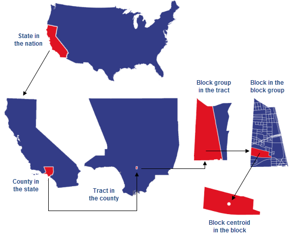\n",
268 | "\n",
269 | "[Source: ESRI](https://learn.arcgis.com/en/related-concepts/united-states-census-geography.htm)"
270 | ]
271 | },
272 | {
273 | "cell_type": "markdown",
274 | "metadata": {
275 | "slideshow": {
276 | "slide_type": "slide"
277 | }
278 | },
279 | "source": [
280 | "## Delete county row\n",
281 | "\n",
282 | "As we have observed, the first row in the data obtained from censusreporter is for the entire county. Keeping this row is problematic, as it represents a data record that is at a different scale. Let's delete it."
283 | ]
284 | },
285 | {
286 | "cell_type": "markdown",
287 | "metadata": {},
288 | "source": [
289 | "
"
67 | ]
68 | },
69 | {
70 | "cell_type": "markdown",
71 | "metadata": {
72 | "slideshow": {
73 | "slide_type": "slide"
74 | }
75 | },
76 | "source": [
77 | "## The libraries"
78 | ]
79 | },
80 | {
81 | "cell_type": "code",
82 | "execution_count": null,
83 | "metadata": {},
84 | "outputs": [],
85 | "source": [
86 | "# to read and visualize spatial data\n",
87 | "import geopandas as gpd\n",
88 | "\n",
89 | "# to provide basemaps \n",
90 | "import contextily as ctx\n",
91 | "\n",
92 | "# to give more power to your figures (plots)\n",
93 | "import matplotlib.pyplot as plt"
94 | ]
95 | },
96 | {
97 | "cell_type": "markdown",
98 | "metadata": {
99 | "slideshow": {
100 | "slide_type": "slide"
101 | }
102 | },
103 | "source": [
104 | "## Importing data\n",
105 | "\n",
106 | "In order to work with data in python, we need a library that will let us handle \"spatial data exploration.\" We looked at shapefiles with geopandas last week, and for this lab, we will use it to read and wrangle a [geojson](https://en.wikipedia.org/wiki/GeoJSON) file.\n",
107 | "\n",
108 | "Before we continue, let's make a brief detour and find out how geojson files are constructed:\n",
109 | "\n",
110 | "- [geojson.io](http://geojson.io/#map=2/20.0/0.0)\n",
111 | "\n",
112 | ""
113 | ]
114 | },
115 | {
116 | "cell_type": "markdown",
117 | "metadata": {
118 | "slideshow": {
119 | "slide_type": "slide"
120 | }
121 | },
122 | "source": [
123 | "We make the call to load and read the data that was downloaded from census reporter. Take note at the relative path reference to find the file in your file directory."
124 | ]
125 | },
126 | {
127 | "cell_type": "code",
128 | "execution_count": null,
129 | "metadata": {},
130 | "outputs": [],
131 | "source": [
132 | "# load a data file\n",
133 | "# note the relative filepath! where is this file located?\n",
134 | "gdf = gpd.read_file('data/acs2019_5yr_B03002_14000US06037534001.geojson')"
135 | ]
136 | },
137 | {
138 | "cell_type": "markdown",
139 | "metadata": {
140 | "slideshow": {
141 | "slide_type": "slide"
142 | }
143 | },
144 | "source": [
145 | "## Preliminary inspection\n",
146 | "A quick look at the size of the data."
147 | ]
148 | },
149 | {
150 | "cell_type": "code",
151 | "execution_count": null,
152 | "metadata": {},
153 | "outputs": [],
154 | "source": [
155 | "# get number of rows, columns\n",
156 | "gdf.shape"
157 | ]
158 | },
159 | {
160 | "cell_type": "code",
161 | "execution_count": null,
162 | "metadata": {
163 | "scrolled": true,
164 | "slideshow": {
165 | "slide_type": "slide"
166 | }
167 | },
168 | "outputs": [],
169 | "source": [
170 | "# get first 5 rows\n",
171 | "gdf.head()"
172 | ]
173 | },
174 | {
175 | "cell_type": "code",
176 | "execution_count": null,
177 | "metadata": {},
178 | "outputs": [],
179 | "source": [
180 | "# get a random row\n",
181 | "gdf.sample()"
182 | ]
183 | },
184 | {
185 | "cell_type": "code",
186 | "execution_count": null,
187 | "metadata": {
188 | "slideshow": {
189 | "slide_type": "slide"
190 | }
191 | },
192 | "outputs": [],
193 | "source": [
194 | "# plot it!\n",
195 | "gdf.plot(figsize=(10,10))"
196 | ]
197 | },
198 | {
199 | "cell_type": "code",
200 | "execution_count": null,
201 | "metadata": {},
202 | "outputs": [],
203 | "source": [
204 | "# plot a random row\n",
205 | "gdf.sample().plot()"
206 | ]
207 | },
208 | {
209 | "cell_type": "markdown",
210 | "metadata": {
211 | "slideshow": {
212 | "slide_type": "slide"
213 | }
214 | },
215 | "source": [
216 | "## Data types\n",
217 | "\n",
218 | "To get the data types, we will use `.info()`. "
219 | ]
220 | },
221 | {
222 | "cell_type": "code",
223 | "execution_count": null,
224 | "metadata": {
225 | "scrolled": true
226 | },
227 | "outputs": [],
228 | "source": [
229 | "# look at columns, null values, and the data types\n",
230 | "gdf.info()"
231 | ]
232 | },
233 | {
234 | "cell_type": "markdown",
235 | "metadata": {
236 | "slideshow": {
237 | "slide_type": "slide"
238 | }
239 | },
240 | "source": [
241 | "### The FIPS code\n",
242 | "What is the geoid? It is called a FIPS code but why is it important?\n",
243 | "\n",
244 | "- https://www.census.gov/programs-surveys/geography/guidance/geo-identifiers.html\n",
245 | "\n",
246 | ""
247 | ]
248 | },
249 | {
250 | "cell_type": "code",
251 | "execution_count": null,
252 | "metadata": {},
253 | "outputs": [],
254 | "source": [
255 | "# get first five geoid's\n",
256 | "gdf.geoid.head()"
257 | ]
258 | },
259 | {
260 | "cell_type": "markdown",
261 | "metadata": {
262 | "slideshow": {
263 | "slide_type": "slide"
264 | }
265 | },
266 | "source": [
267 | "\n",
268 | "\n",
269 | "[Source: ESRI](https://learn.arcgis.com/en/related-concepts/united-states-census-geography.htm)"
270 | ]
271 | },
272 | {
273 | "cell_type": "markdown",
274 | "metadata": {
275 | "slideshow": {
276 | "slide_type": "slide"
277 | }
278 | },
279 | "source": [
280 | "## Delete county row\n",
281 | "\n",
282 | "As we have observed, the first row in the data obtained from censusreporter is for the entire county. Keeping this row is problematic, as it represents a data record that is at a different scale. Let's delete it."
283 | ]
284 | },
285 | {
286 | "cell_type": "markdown",
287 | "metadata": {},
288 | "source": [
289 | "\n",
290 | " Important!
\n",
291 | " Note that any data downloaded from censusreporter will have a \"summary row\" for the entire data.\n",
292 | ""
293 | ]
294 | },
295 | {
296 | "cell_type": "code",
297 | "execution_count": null,
298 | "metadata": {
299 | "slideshow": {
300 | "slide_type": "slide"
301 | }
302 | },
303 | "outputs": [],
304 | "source": [
305 | "# check the data again\n",
306 | "gdf.head()"
307 | ]
308 | },
309 | {
310 | "cell_type": "code",
311 | "execution_count": null,
312 | "metadata": {
313 | "slideshow": {
314 | "slide_type": "slide"
315 | }
316 | },
317 | "outputs": [],
318 | "source": [
319 | "# drop the row with index 0 (i.e. the first row)\n",
320 | "gdf = gdf.drop([0])"
321 | ]
322 | },
323 | {
324 | "cell_type": "code",
325 | "execution_count": null,
326 | "metadata": {
327 | "slideshow": {
328 | "slide_type": "fragment"
329 | }
330 | },
331 | "outputs": [],
332 | "source": [
333 | "# check to see if it has been deleted\n",
334 | "gdf.head()"
335 | ]
336 | },
337 | {
338 | "cell_type": "markdown",
339 | "metadata": {
340 | "slideshow": {
341 | "slide_type": "slide"
342 | }
343 | },
344 | "source": [
345 | "## The census data dictionary\n",
346 | "There are a lot of columns. What are these columns? Column headers are defined in the `metadata.json` file that comes in the dowloaded zipfile from censusreporter. Click the link below to open the json file in another tab.\n",
347 | "\n",
348 | "* [metadata.json](data/metadata.json)"
349 | ]
350 | },
351 | {
352 | "cell_type": "markdown",
353 | "metadata": {
354 | "slideshow": {
355 | "slide_type": "slide"
356 | }
357 | },
358 | "source": [
359 | "Let's identify which columns are needed, and which are not for our exploration.\n",
360 | "\n",
361 | ""
362 | ]
363 | },
364 | {
365 | "cell_type": "markdown",
366 | "metadata": {
367 | "slideshow": {
368 | "slide_type": "slide"
369 | }
370 | },
371 | "source": [
372 | "## Dropping columns \n",
373 | "There are many columns that we do not need. \n",
374 | "\n",
375 | "- output existing columns as a list\n",
376 | "- create a list of columns to keep\n",
377 | "- redefine `gdf` with only the columns to keep\n"
378 | ]
379 | },
380 | {
381 | "cell_type": "code",
382 | "execution_count": null,
383 | "metadata": {
384 | "scrolled": true,
385 | "slideshow": {
386 | "slide_type": "slide"
387 | }
388 | },
389 | "outputs": [],
390 | "source": [
391 | "list(gdf) # this is the same as df.columns.to_list()"
392 | ]
393 | },
394 | {
395 | "cell_type": "code",
396 | "execution_count": null,
397 | "metadata": {
398 | "slideshow": {
399 | "slide_type": "slide"
400 | }
401 | },
402 | "outputs": [],
403 | "source": [
404 | "# create a list of columns to keep\n",
405 | "columns_to_keep = ['geoid',\n",
406 | " 'name',\n",
407 | " 'B03002001',\n",
408 | " 'B03002002',\n",
409 | " 'B03002003',\n",
410 | " 'B03002004',\n",
411 | " 'B03002005',\n",
412 | " 'B03002006',\n",
413 | " 'B03002007',\n",
414 | " 'B03002008',\n",
415 | " 'B03002009',\n",
416 | " 'B03002012',\n",
417 | " 'geometry']"
418 | ]
419 | },
420 | {
421 | "cell_type": "code",
422 | "execution_count": null,
423 | "metadata": {
424 | "slideshow": {
425 | "slide_type": "slide"
426 | }
427 | },
428 | "outputs": [],
429 | "source": [
430 | "# redefine gdf with only columns to keep\n",
431 | "gdf = gdf[columns_to_keep]"
432 | ]
433 | },
434 | {
435 | "cell_type": "code",
436 | "execution_count": null,
437 | "metadata": {
438 | "scrolled": true,
439 | "slideshow": {
440 | "slide_type": "fragment"
441 | }
442 | },
443 | "outputs": [],
444 | "source": [
445 | "# check the slimmed down gdf\n",
446 | "gdf.head()"
447 | ]
448 | },
449 | {
450 | "cell_type": "markdown",
451 | "metadata": {
452 | "slideshow": {
453 | "slide_type": "slide"
454 | }
455 | },
456 | "source": [
457 | "## Renaming columns\n",
458 | "\n",
459 | "Let's rename the columns. First, create a list of column names as they are now."
460 | ]
461 | },
462 | {
463 | "cell_type": "code",
464 | "execution_count": null,
465 | "metadata": {},
466 | "outputs": [],
467 | "source": [
468 | "list(gdf) # this is the same as df.columns.to_list()"
469 | ]
470 | },
471 | {
472 | "cell_type": "markdown",
473 | "metadata": {
474 | "slideshow": {
475 | "slide_type": "slide"
476 | }
477 | },
478 | "source": [
479 | "Then, simply copy and paste the output list above, and define the columns with it. Replace the values with your desired column names"
480 | ]
481 | },
482 | {
483 | "cell_type": "code",
484 | "execution_count": null,
485 | "metadata": {},
486 | "outputs": [],
487 | "source": [
488 | "gdf.columns = ['geoid',\n",
489 | " 'name',\n",
490 | " 'Total',\n",
491 | " 'Non Hispanic',\n",
492 | " 'Non Hispanic White',\n",
493 | " 'Non Hispanic Black',\n",
494 | " 'Non Hispanic American Indian and Alaska Native',\n",
495 | " 'Non Hispanic Asian',\n",
496 | " 'Non Hispanic Native Hawaiian and Other Pacific Islander',\n",
497 | " 'Non Hispanic Some other race',\n",
498 | " 'Non Hispanic Two or more races',\n",
499 | " 'Hispanic',\n",
500 | " 'geometry']"
501 | ]
502 | },
503 | {
504 | "cell_type": "code",
505 | "execution_count": null,
506 | "metadata": {
507 | "slideshow": {
508 | "slide_type": "slide"
509 | }
510 | },
511 | "outputs": [],
512 | "source": [
513 | "# check the renamed columns\n",
514 | "gdf.head()"
515 | ]
516 | },
517 | {
518 | "cell_type": "markdown",
519 | "metadata": {
520 | "slideshow": {
521 | "slide_type": "slide"
522 | }
523 | },
524 | "source": [
525 | "## Double check your data integrity\n",
526 | "Does the math add up? Let's check. The `Total` should equal the rest of the columns."
527 | ]
528 | },
529 | {
530 | "cell_type": "code",
531 | "execution_count": null,
532 | "metadata": {
533 | "slideshow": {
534 | "slide_type": "fragment"
535 | }
536 | },
537 | "outputs": [],
538 | "source": [
539 | "# get a random record\n",
540 | "random_tract = gdf.sample()\n",
541 | "random_tract"
542 | ]
543 | },
544 | {
545 | "cell_type": "markdown",
546 | "metadata": {
547 | "slideshow": {
548 | "slide_type": "slide"
549 | }
550 | },
551 | "source": [
552 | "To get values from individual cells in a dataframe, use the `iloc` command.\n",
553 | "\n",
554 | "- `iloc` ([documentation](https://pandas.pydata.org/pandas-docs/stable/reference/api/pandas.DataFrame.iloc.html))\n",
555 | "\n",
556 | "While there are various methods to get cell values in python, the iloc command allows you to get to a cell based on the position of the record row and the column name."
557 | ]
558 | },
559 | {
560 | "cell_type": "code",
561 | "execution_count": null,
562 | "metadata": {
563 | "slideshow": {
564 | "slide_type": "slide"
565 | }
566 | },
567 | "outputs": [],
568 | "source": [
569 | "# example usage of iloc to get the total population of our random record\n",
570 | "# \"for the 0th record, get the value in the Total column\"\n",
571 | "random_tract.iloc[0]['Total']"
572 | ]
573 | },
574 | {
575 | "cell_type": "code",
576 | "execution_count": null,
577 | "metadata": {
578 | "slideshow": {
579 | "slide_type": "fragment"
580 | }
581 | },
582 | "outputs": [],
583 | "source": [
584 | "# print this out in plain english\n",
585 | "print('Total population: ' + str(random_tract.iloc[0]['Total']))"
586 | ]
587 | },
588 | {
589 | "cell_type": "code",
590 | "execution_count": null,
591 | "metadata": {},
592 | "outputs": [],
593 | "source": [
594 | "# non hispanic plus hispanic should equal to the total\n",
595 | "print('Non Hispanic + Hispanic: ' + str(random_tract.iloc[0]['Non Hispanic'] + random_tract.iloc[0]['Hispanic']))"
596 | ]
597 | },
598 | {
599 | "cell_type": "code",
600 | "execution_count": null,
601 | "metadata": {},
602 | "outputs": [],
603 | "source": [
604 | "# hispanic plus all the non hispanice categories\n",
605 | "print(random_tract.iloc[0]['Non Hispanic White'] + \n",
606 | " random_tract.iloc[0]['Non Hispanic Black'] + \n",
607 | " random_tract.iloc[0]['Non Hispanic American Indian and Alaska Native'] + \n",
608 | " random_tract.iloc[0]['Non Hispanic Asian'] + \n",
609 | " random_tract.iloc[0]['Non Hispanic Native Hawaiian and Other Pacific Islander'] + \n",
610 | " random_tract.iloc[0]['Non Hispanic Some other race'] + \n",
611 | " random_tract.iloc[0]['Non Hispanic Two or more races'] + \n",
612 | " random_tract.iloc[0]['Hispanic'])"
613 | ]
614 | },
615 | {
616 | "cell_type": "markdown",
617 | "metadata": {
618 | "slideshow": {
619 | "slide_type": "slide"
620 | }
621 | },
622 | "source": [
623 | "## Simple stats and plots"
624 | ]
625 | },
626 | {
627 | "cell_type": "code",
628 | "execution_count": null,
629 | "metadata": {
630 | "scrolled": true
631 | },
632 | "outputs": [],
633 | "source": [
634 | "# access a single column like df['col_name']\n",
635 | "gdf['Total'].head()"
636 | ]
637 | },
638 | {
639 | "cell_type": "code",
640 | "execution_count": null,
641 | "metadata": {
642 | "slideshow": {
643 | "slide_type": "slide"
644 | }
645 | },
646 | "outputs": [],
647 | "source": [
648 | "# What is the mean?\n",
649 | "gdf['Total'].mean()"
650 | ]
651 | },
652 | {
653 | "cell_type": "code",
654 | "execution_count": null,
655 | "metadata": {},
656 | "outputs": [],
657 | "source": [
658 | "# What is the median?\n",
659 | "gdf['Total'].median()"
660 | ]
661 | },
662 | {
663 | "cell_type": "code",
664 | "execution_count": null,
665 | "metadata": {},
666 | "outputs": [],
667 | "source": [
668 | "# get some stats\n",
669 | "gdf['Total'].describe()"
670 | ]
671 | },
672 | {
673 | "cell_type": "markdown",
674 | "metadata": {
675 | "slideshow": {
676 | "slide_type": "slide"
677 | }
678 | },
679 | "source": [
680 | "## Create your first plot\n",
681 | "\n",
682 | "- https://pandas.pydata.org/pandas-docs/stable/user_guide/visualization.html"
683 | ]
684 | },
685 | {
686 | "cell_type": "code",
687 | "execution_count": null,
688 | "metadata": {
689 | "scrolled": true,
690 | "slideshow": {
691 | "slide_type": "slide"
692 | }
693 | },
694 | "outputs": [],
695 | "source": [
696 | "# plot it as a historgram with 50 bins\n",
697 | "gdf['Total'].plot.hist()"
698 | ]
699 | },
700 | {
701 | "cell_type": "code",
702 | "execution_count": null,
703 | "metadata": {
704 | "scrolled": true,
705 | "slideshow": {
706 | "slide_type": "slide"
707 | }
708 | },
709 | "outputs": [],
710 | "source": [
711 | "# make it bigger, increase the number of bins, and give it a title\n",
712 | "gdf['Total'].plot.hist(figsize=(12,5),\n",
713 | " bins=100,\n",
714 | " title='Los Angeles County census tracts by population size (ACS 2019 5-year)')"
715 | ]
716 | },
717 | {
718 | "cell_type": "markdown",
719 | "metadata": {
720 | "slideshow": {
721 | "slide_type": "slide"
722 | }
723 | },
724 | "source": [
725 | "\n",
726 | " Now it's your turn. Find some stats for different fields in the data and output them below.\n",
727 | "
"
728 | ]
729 | },
730 | {
731 | "cell_type": "code",
732 | "execution_count": null,
733 | "metadata": {},
734 | "outputs": [],
735 | "source": []
736 | },
737 | {
738 | "cell_type": "markdown",
739 | "metadata": {
740 | "slideshow": {
741 | "slide_type": "slide"
742 | }
743 | },
744 | "source": [
745 | "## Sorting\n",
746 | "What are the top 10 most populated census tracts? What are the census tracts with the highest black popluation? To answer these questions, the simplest method is to sort the data by their respective columns.\n",
747 | "\n",
748 | "- [pandas sort_values](https://pandas.pydata.org/pandas-docs/stable/reference/api/pandas.DataFrame.sort_values.html)"
749 | ]
750 | },
751 | {
752 | "cell_type": "code",
753 | "execution_count": null,
754 | "metadata": {},
755 | "outputs": [],
756 | "source": [
757 | "gdf_sorted = gdf.sort_values(by='Total',ascending = False)"
758 | ]
759 | },
760 | {
761 | "cell_type": "code",
762 | "execution_count": null,
763 | "metadata": {
764 | "scrolled": true,
765 | "slideshow": {
766 | "slide_type": "slide"
767 | }
768 | },
769 | "outputs": [],
770 | "source": [
771 | "# display the data, but just a few columns to keep it clean\n",
772 | "gdf_sorted[['geoid','Total']].head(10)"
773 | ]
774 | },
775 | {
776 | "cell_type": "code",
777 | "execution_count": null,
778 | "metadata": {
779 | "slideshow": {
780 | "slide_type": "slide"
781 | }
782 | },
783 | "outputs": [],
784 | "source": [
785 | "# plot the top 10 most populated tracts\n",
786 | "gdf_sorted.head(10).plot(figsize=(10,10))"
787 | ]
788 | },
789 | {
790 | "cell_type": "code",
791 | "execution_count": null,
792 | "metadata": {
793 | "slideshow": {
794 | "slide_type": "slide"
795 | }
796 | },
797 | "outputs": [],
798 | "source": [
799 | "# Make it 100 and prettier\n",
800 | "gdf_sorted.head(1000).plot(figsize=(10,10),\n",
801 | " column='Total', \n",
802 | " cmap='plasma', \n",
803 | " legend=True)"
804 | ]
805 | },
806 | {
807 | "cell_type": "markdown",
808 | "metadata": {
809 | "slideshow": {
810 | "slide_type": "slide"
811 | }
812 | },
813 | "source": [
814 | "\n",
815 | "Now it's your turn! Create a table and accompanying bar plot for the top/bottom x values for column of your choice.\n",
816 | "
"
817 | ]
818 | },
819 | {
820 | "cell_type": "code",
821 | "execution_count": null,
822 | "metadata": {},
823 | "outputs": [],
824 | "source": []
825 | },
826 | {
827 | "cell_type": "markdown",
828 | "metadata": {
829 | "slideshow": {
830 | "slide_type": "slide"
831 | }
832 | },
833 | "source": [
834 | "## Filtering and subsetting data\n",
835 | "Sorting is one method, but the process of discovery compels us to interrogate the data in different ways. One method of doing so is to query, or filter the data to see specific views of the data based on a question you may have. For example, what are the census tract that have no people in them? Or, Which census tracts are more than 75% black?"
836 | ]
837 | },
838 | {
839 | "cell_type": "code",
840 | "execution_count": null,
841 | "metadata": {
842 | "jupyter": {
843 | "outputs_hidden": true
844 | },
845 | "scrolled": true,
846 | "slideshow": {
847 | "slide_type": "slide"
848 | }
849 | },
850 | "outputs": [],
851 | "source": [
852 | "# subset the data so that we can see the data per row... \n",
853 | "# in other words, this syntax is asking to \"show me the values in my dataframe that match this filter\n",
854 | "gdf[gdf['Total']==0]"
855 | ]
856 | },
857 | {
858 | "cell_type": "markdown",
859 | "metadata": {
860 | "slideshow": {
861 | "slide_type": "slide"
862 | }
863 | },
864 | "source": [
865 | "Note that unless you specify the resulting output as a new variable, the results are only temporary (in memory). If you want to use the results for subsequent analysis, you need to create a new variable."
866 | ]
867 | },
868 | {
869 | "cell_type": "code",
870 | "execution_count": null,
871 | "metadata": {},
872 | "outputs": [],
873 | "source": [
874 | "# create a new variable for census tracts with zero pop\n",
875 | "gdf_no_pop = gdf[gdf['Total']==0]"
876 | ]
877 | },
878 | {
879 | "cell_type": "code",
880 | "execution_count": null,
881 | "metadata": {
882 | "slideshow": {
883 | "slide_type": "slide"
884 | }
885 | },
886 | "outputs": [],
887 | "source": [
888 | "# how many records?\n",
889 | "print('There are ' + str(len(gdf_no_pop)) + ' census tracts with no people in them')"
890 | ]
891 | },
892 | {
893 | "cell_type": "code",
894 | "execution_count": null,
895 | "metadata": {
896 | "scrolled": false,
897 | "slideshow": {
898 | "slide_type": "fragment"
899 | }
900 | },
901 | "outputs": [],
902 | "source": [
903 | "# display it\n",
904 | "gdf_no_pop[['geoid','Total']]"
905 | ]
906 | },
907 | {
908 | "cell_type": "markdown",
909 | "metadata": {
910 | "slideshow": {
911 | "slide_type": "slide"
912 | }
913 | },
914 | "source": [
915 | "## Totals are great but let's normalize the data\n",
916 | "\n",
917 | "For almost any data inquiry, you should ask the question: should I normalize the data? With raw numbers, is it fair to compare one census tract to another? For example, if one census tract has 1000 hispanics, and another has 100, can we assume that the first tract is largely Hispanic? No, because the total population might be 10000 people, resulting in it being 10% hispanic, whereas the second tract might have 200 people living in it, resulting in it being 50% hispanic."
918 | ]
919 | },
920 | {
921 | "cell_type": "markdown",
922 | "metadata": {
923 | "slideshow": {
924 | "slide_type": "slide"
925 | }
926 | },
927 | "source": [
928 | "To avoid these types of misrepresentations, we can normalize the data, and provide it as a percent of total."
929 | ]
930 | },
931 | {
932 | "cell_type": "code",
933 | "execution_count": null,
934 | "metadata": {
935 | "slideshow": {
936 | "slide_type": "fragment"
937 | }
938 | },
939 | "outputs": [],
940 | "source": [
941 | "# output columns\n",
942 | "list(gdf)"
943 | ]
944 | },
945 | {
946 | "cell_type": "code",
947 | "execution_count": null,
948 | "metadata": {
949 | "slideshow": {
950 | "slide_type": "slide"
951 | }
952 | },
953 | "outputs": [],
954 | "source": [
955 | "# create a new column, and populate it with normalized data to get the percent of total value\n",
956 | "gdf['Percent Non Hispanic'] = gdf['Non Hispanic']/gdf['Total']*100\n",
957 | "gdf['Percent Hispanic'] = gdf['Hispanic']/gdf['Total']*100"
958 | ]
959 | },
960 | {
961 | "cell_type": "code",
962 | "execution_count": null,
963 | "metadata": {
964 | "scrolled": false,
965 | "slideshow": {
966 | "slide_type": "fragment"
967 | }
968 | },
969 | "outputs": [],
970 | "source": [
971 | "gdf.sample(5)"
972 | ]
973 | },
974 | {
975 | "cell_type": "markdown",
976 | "metadata": {
977 | "slideshow": {
978 | "slide_type": "slide"
979 | }
980 | },
981 | "source": [
982 | "### Now it's your turn!\n",
983 | "\n",
984 | "Now it's your turn! Create new columns for \n",
985 | "- `Percent Non Hispanic White`\n",
986 | "- `Percent Non Hispanic Black`\n",
987 | "- `Percent Non Hispanic American Indian and Alaska Native`\n",
988 | "- `Percent Non Hispanic Asian`\n",
989 | "- `Percent Non Hispanic Native Hawaiian and Other Pacific Islander`\n",
990 | "- `Percent Non Hispanic Some other race`\n",
991 | "- `Percent Non Hispanic Two or more races`"
992 | ]
993 | },
994 | {
995 | "cell_type": "code",
996 | "execution_count": null,
997 | "metadata": {},
998 | "outputs": [],
999 | "source": []
1000 | },
1001 | {
1002 | "cell_type": "markdown",
1003 | "metadata": {
1004 | "slideshow": {
1005 | "slide_type": "slide"
1006 | }
1007 | },
1008 | "source": [
1009 | "# Maps!"
1010 | ]
1011 | },
1012 | {
1013 | "cell_type": "markdown",
1014 | "metadata": {
1015 | "slideshow": {
1016 | "slide_type": "slide"
1017 | }
1018 | },
1019 | "source": [
1020 | "We can now create choropleth maps in geopandas. \n",
1021 | "\n",
1022 | "* [geopandas choropleth maps](https://geopandas.org/mapping.html#choropleth-maps)\n",
1023 | "* [color schemes with mapclassify](https://pysal.org/notebooks/viz/mapclassify/intro.html)\n",
1024 | " * `natural_breaks`\n",
1025 | " * `equal_interval`\n",
1026 | " * `quantiles`\n",
1027 | " * etc..."
1028 | ]
1029 | },
1030 | {
1031 | "cell_type": "code",
1032 | "execution_count": null,
1033 | "metadata": {
1034 | "slideshow": {
1035 | "slide_type": "slide"
1036 | }
1037 | },
1038 | "outputs": [],
1039 | "source": [
1040 | "gdf.plot(figsize=(12,10),\n",
1041 | " column='Percent Hispanic',\n",
1042 | " legend=True, \n",
1043 | " scheme='NaturalBreaks')"
1044 | ]
1045 | },
1046 | {
1047 | "cell_type": "code",
1048 | "execution_count": null,
1049 | "metadata": {
1050 | "scrolled": false,
1051 | "slideshow": {
1052 | "slide_type": "slide"
1053 | }
1054 | },
1055 | "outputs": [],
1056 | "source": [
1057 | "gdf.plot(figsize=(12,10),\n",
1058 | " column='Percent Hispanic',\n",
1059 | " legend=True, \n",
1060 | " scheme='equal_interval')"
1061 | ]
1062 | },
1063 | {
1064 | "cell_type": "code",
1065 | "execution_count": null,
1066 | "metadata": {
1067 | "scrolled": false,
1068 | "slideshow": {
1069 | "slide_type": "slide"
1070 | }
1071 | },
1072 | "outputs": [],
1073 | "source": [
1074 | "gdf.plot(figsize=(12,10),\n",
1075 | " column='Percent Hispanic',\n",
1076 | " legend=True, \n",
1077 | " scheme='quantiles')"
1078 | ]
1079 | },
1080 | {
1081 | "cell_type": "markdown",
1082 | "metadata": {
1083 | "slideshow": {
1084 | "slide_type": "slide"
1085 | }
1086 | },
1087 | "source": [
1088 | "## Using subplots to create multiple plots\n",
1089 | "\n",
1090 | "It is often useful to generate multiple plots next to each other. To do so, we look at matplotlib's `subplot` command:\n",
1091 | "\n",
1092 | "- https://matplotlib.org/3.3.3/api/_as_gen/matplotlib.pyplot.subplots.html"
1093 | ]
1094 | },
1095 | {
1096 | "cell_type": "code",
1097 | "execution_count": null,
1098 | "metadata": {
1099 | "slideshow": {
1100 | "slide_type": "slide"
1101 | }
1102 | },
1103 | "outputs": [],
1104 | "source": [
1105 | "# create the 1x2 subplots\n",
1106 | "fig, axs = plt.subplots(1, 2, figsize=(15, 12))\n",
1107 | "\n",
1108 | "# name each subplot\n",
1109 | "ax1, ax2 = axs\n",
1110 | "\n",
1111 | "# regular count map on the left\n",
1112 | "gdf.plot(column='Percent Hispanic', \n",
1113 | " cmap='RdYlGn_r', \n",
1114 | " scheme='quantiles',\n",
1115 | " k=5, \n",
1116 | " edgecolor='white', \n",
1117 | " linewidth=0., \n",
1118 | " alpha=0.75, \n",
1119 | " ax=ax1, # this assigns the map to the subplot,\n",
1120 | " legend=True\n",
1121 | " )\n",
1122 | "\n",
1123 | "ax1.axis(\"off\")\n",
1124 | "ax1.set_title(\"Percent Hispanic\")\n",
1125 | "\n",
1126 | "# spatial lag map on the right\n",
1127 | "gdf.plot(column='Percent Non Hispanic Black', \n",
1128 | " cmap='RdYlGn_r', \n",
1129 | " scheme='quantiles',\n",
1130 | " k=5, \n",
1131 | " edgecolor='white', \n",
1132 | " linewidth=0., \n",
1133 | " alpha=0.75, \n",
1134 | " ax=ax2, # this assigns the map to the subplot\n",
1135 | " legend=True\n",
1136 | " )\n",
1137 | "\n",
1138 | "ax2.axis(\"off\")\n",
1139 | "ax2.set_title(\"Percent Non Hispanic Black\")"
1140 | ]
1141 | },
1142 | {
1143 | "cell_type": "markdown",
1144 | "metadata": {
1145 | "slideshow": {
1146 | "slide_type": "slide"
1147 | }
1148 | },
1149 | "source": [
1150 | "\n",
1151 | "\n",
1152 | "Now it's your turn! Create map plots based on other race indicators. Experiment with the different schemes to display variations of the same data, mapped differently.\n",
1153 | "\n",
1154 | "
"
1155 | ]
1156 | },
1157 | {
1158 | "cell_type": "code",
1159 | "execution_count": null,
1160 | "metadata": {},
1161 | "outputs": [],
1162 | "source": []
1163 | },
1164 | {
1165 | "cell_type": "markdown",
1166 | "metadata": {
1167 | "slideshow": {
1168 | "slide_type": "slide"
1169 | }
1170 | },
1171 | "source": [
1172 | "## Additional mapping ideas\n",
1173 | "What does the majority ethnic cluster look like in Los Angeles?"
1174 | ]
1175 | },
1176 | {
1177 | "cell_type": "code",
1178 | "execution_count": null,
1179 | "metadata": {},
1180 | "outputs": [],
1181 | "source": [
1182 | "gdf[gdf['Percent Hispanic'] > 80]"
1183 | ]
1184 | },
1185 | {
1186 | "cell_type": "code",
1187 | "execution_count": null,
1188 | "metadata": {
1189 | "scrolled": false,
1190 | "slideshow": {
1191 | "slide_type": "slide"
1192 | }
1193 | },
1194 | "outputs": [],
1195 | "source": [
1196 | "gdf[gdf['Percent Hispanic'] > 90].plot(figsize=(12,10))"
1197 | ]
1198 | },
1199 | {
1200 | "cell_type": "markdown",
1201 | "metadata": {
1202 | "slideshow": {
1203 | "slide_type": "slide"
1204 | }
1205 | },
1206 | "source": [
1207 | "\n",
1208 | "\n",
1209 | "Now it's your turn! Create map plots based on other race indicators with varying segments of the population.\n",
1210 | "\n",
1211 | "
"
1212 | ]
1213 | },
1214 | {
1215 | "cell_type": "code",
1216 | "execution_count": null,
1217 | "metadata": {},
1218 | "outputs": [],
1219 | "source": []
1220 | },
1221 | {
1222 | "cell_type": "markdown",
1223 | "metadata": {
1224 | "slideshow": {
1225 | "slide_type": "slide"
1226 | }
1227 | },
1228 | "source": [
1229 | "## Add a basemap\n",
1230 | "\n",
1231 | "Adding a basemap to a geopandas plot can be done using the [contextily library](https://contextily.readthedocs.io/en/latest/intro_guide.html). To do so, you must:\n",
1232 | "\n",
1233 | "* reproject your geodataframe to Web Mercator (epsg: 3857)\n",
1234 | "* add a basemap, use the following [guidelines](https://github.com/geopandas/contextily/blob/master/notebooks/providers_deepdive.ipynb)"
1235 | ]
1236 | },
1237 | {
1238 | "cell_type": "markdown",
1239 | "metadata": {
1240 | "slideshow": {
1241 | "slide_type": "slide"
1242 | }
1243 | },
1244 | "source": [
1245 | "### Project to web mercator\n",
1246 | "\n",
1247 | "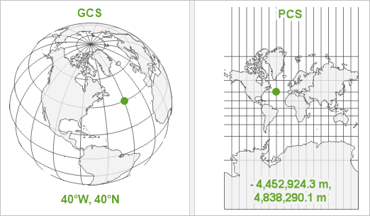\n",
1248 | "\n",
1249 | "In order to conduct spatial analysis, it is recommended to use a projected coordinate system, rather than a geographic coordinate system (which uses angular measurements). Here is an [blog post from ESRI](https://www.esri.com/arcgis-blog/products/arcgis-pro/mapping/gcs_vs_pcs/) that describes the differences between the two."
1250 | ]
1251 | },
1252 | {
1253 | "cell_type": "code",
1254 | "execution_count": null,
1255 | "metadata": {
1256 | "slideshow": {
1257 | "slide_type": "slide"
1258 | }
1259 | },
1260 | "outputs": [],
1261 | "source": [
1262 | "# reproject to Web Mercator\n",
1263 | "gdf_web_mercator = gdf.to_crs(epsg=3857)\n",
1264 | "gdf_web_mercator"
1265 | ]
1266 | },
1267 | {
1268 | "cell_type": "code",
1269 | "execution_count": null,
1270 | "metadata": {
1271 | "slideshow": {
1272 | "slide_type": "slide"
1273 | }
1274 | },
1275 | "outputs": [],
1276 | "source": [
1277 | "# use subplots that make it easier to create multiple layered maps\n",
1278 | "fig, ax = plt.subplots(figsize=(15, 15))\n",
1279 | "\n",
1280 | "# add the layer with ax=ax in the argument \n",
1281 | "gdf_web_mercator[gdf_web_mercator['Percent Hispanic'] > 50].plot(ax=ax, alpha=0.8)\n",
1282 | "\n",
1283 | "# turn the axis off\n",
1284 | "ax.axis('off')\n",
1285 | "\n",
1286 | "# set a title\n",
1287 | "ax.set_title('Census Tracts with more than 50% Hispanic Population',fontsize=16)\n",
1288 | "\n",
1289 | "# add a basemap\n",
1290 | "ctx.add_basemap(ax)"
1291 | ]
1292 | }
1293 | ],
1294 | "metadata": {
1295 | "celltoolbar": "Slideshow",
1296 | "kernelspec": {
1297 | "display_name": "Python 3",
1298 | "language": "python",
1299 | "name": "python3"
1300 | },
1301 | "language_info": {
1302 | "codemirror_mode": {
1303 | "name": "ipython",
1304 | "version": 3
1305 | },
1306 | "file_extension": ".py",
1307 | "mimetype": "text/x-python",
1308 | "name": "python",
1309 | "nbconvert_exporter": "python",
1310 | "pygments_lexer": "ipython3",
1311 | "version": "3.8.5"
1312 | },
1313 | "toc": {
1314 | "base_numbering": 1,
1315 | "nav_menu": {},
1316 | "number_sections": true,
1317 | "sideBar": true,
1318 | "skip_h1_title": false,
1319 | "title_cell": "Table of Contents",
1320 | "title_sidebar": "Contents",
1321 | "toc_cell": true,
1322 | "toc_position": {
1323 | "height": "calc(100% - 180px)",
1324 | "left": "10px",
1325 | "top": "150px",
1326 | "width": "350.797px"
1327 | },
1328 | "toc_section_display": true,
1329 | "toc_window_display": false
1330 | }
1331 | },
1332 | "nbformat": 4,
1333 | "nbformat_minor": 4
1334 | }
1335 |
--------------------------------------------------------------------------------
/Intro to GIS.ipynb:
--------------------------------------------------------------------------------
1 | {
2 | "cells": [
3 | {
4 | "cell_type": "markdown",
5 | "metadata": {
6 | "toc": true
7 | },
8 | "source": [
9 | "Table of Contents
\n",
10 | ""
11 | ]
12 | },
13 | {
14 | "cell_type": "markdown",
15 | "metadata": {
16 | "slideshow": {
17 | "slide_type": "slide"
18 | }
19 | },
20 | "source": [
21 | "\n",
22 | "\n",
23 | "
Take notice!
\n",
24 | "
\n",
25 | " - This class will be recorded
\n",
26 | "
\n",
27 | " \n",
28 | "
 \n",
246 | "\n",
247 | "Source: [New York Times,\n",
248 | "2020](https://www.nytimes.com/interactive/2020/11/03/us/elections/results-president.html)\n",
249 | "\n",
250 | "The states themselves are the boundaries, even though the data is\n",
251 | "collected at smaller levels.\n",
252 | "\n",
253 | "How is that possible? "
254 | ]
255 | },
256 | {
257 | "cell_type": "markdown",
258 | "metadata": {
259 | "slideshow": {
260 | "slide_type": "slide"
261 | }
262 | },
263 | "source": [
264 | "### Geographic Hierarchy\n",
265 | "\n",
266 | "Move over Aristotle: The **sum** is the whole of its parts!\n",
267 | "\n",
268 | "The first law of Geography (and perhaps only) is \"**everything is\n",
269 | "related to everything else, but nearer things are more related than\n",
270 | "distant things.**\" When thinking about human data, there are many\n",
271 | "different units, countries, states, cities, and even households.\n",
272 | "Whenever this data is being summarized to larger geographies, as long as\n",
273 | "the smaller boundaries do not overlap then you can do so. However, this\n",
274 | "does not mean it is always safe to do so, why?"
275 | ]
276 | },
277 | {
278 | "cell_type": "markdown",
279 | "metadata": {
280 | "slideshow": {
281 | "slide_type": "slide"
282 | }
283 | },
284 | "source": [
285 | "Keeping the first law of geography in mind, when you summarize smaller\n",
286 | "data to larger geographies (i.e. going from cities to a state), the\n",
287 | "nearer things become less related because they are summarized to a\n",
288 | "larger geographic relation. Let's return to the election map, but\n",
289 | "break it down into counties to see how the summing of the data changed\n",
290 | "spatial relationships.\n",
291 | "\n",
292 | "
\n",
246 | "\n",
247 | "Source: [New York Times,\n",
248 | "2020](https://www.nytimes.com/interactive/2020/11/03/us/elections/results-president.html)\n",
249 | "\n",
250 | "The states themselves are the boundaries, even though the data is\n",
251 | "collected at smaller levels.\n",
252 | "\n",
253 | "How is that possible? "
254 | ]
255 | },
256 | {
257 | "cell_type": "markdown",
258 | "metadata": {
259 | "slideshow": {
260 | "slide_type": "slide"
261 | }
262 | },
263 | "source": [
264 | "### Geographic Hierarchy\n",
265 | "\n",
266 | "Move over Aristotle: The **sum** is the whole of its parts!\n",
267 | "\n",
268 | "The first law of Geography (and perhaps only) is \"**everything is\n",
269 | "related to everything else, but nearer things are more related than\n",
270 | "distant things.**\" When thinking about human data, there are many\n",
271 | "different units, countries, states, cities, and even households.\n",
272 | "Whenever this data is being summarized to larger geographies, as long as\n",
273 | "the smaller boundaries do not overlap then you can do so. However, this\n",
274 | "does not mean it is always safe to do so, why?"
275 | ]
276 | },
277 | {
278 | "cell_type": "markdown",
279 | "metadata": {
280 | "slideshow": {
281 | "slide_type": "slide"
282 | }
283 | },
284 | "source": [
285 | "Keeping the first law of geography in mind, when you summarize smaller\n",
286 | "data to larger geographies (i.e. going from cities to a state), the\n",
287 | "nearer things become less related because they are summarized to a\n",
288 | "larger geographic relation. Let's return to the election map, but\n",
289 | "break it down into counties to see how the summing of the data changed\n",
290 | "spatial relationships.\n",
291 | "\n",
292 | " \n",
293 | "\n",
294 | "\n",
295 | "Source: [USA Today,\n",
296 | "2020](https://www.usatoday.com/in-depth/graphics/2020/11/10/election-maps-2020-america-county-results-more-voters/6226197002/#mainContentSection)"
297 | ]
298 | },
299 | {
300 | "cell_type": "markdown",
301 | "metadata": {
302 | "slideshow": {
303 | "slide_type": "slide"
304 | }
305 | },
306 | "source": [
307 | "How does this map compare to the previous map?\n",
308 | "\n",
309 | "\n",
310 | "\n",
311 | "For one thing, you can see that a state like Nevada is not completely blue and has quite a bit of Republican voters. When a whole state is considered “democrat” or blue, such types of simplifications can only occur when data from the counties is summarized upwards to the state level."
312 | ]
313 | },
314 | {
315 | "cell_type": "markdown",
316 | "metadata": {
317 | "slideshow": {
318 | "slide_type": "slide"
319 | }
320 | },
321 | "source": [
322 | "Below is an example of how the United States Census Bureau’s uses hierarchal geography: \n",
323 | "\n",
324 | "
\n",
293 | "\n",
294 | "\n",
295 | "Source: [USA Today,\n",
296 | "2020](https://www.usatoday.com/in-depth/graphics/2020/11/10/election-maps-2020-america-county-results-more-voters/6226197002/#mainContentSection)"
297 | ]
298 | },
299 | {
300 | "cell_type": "markdown",
301 | "metadata": {
302 | "slideshow": {
303 | "slide_type": "slide"
304 | }
305 | },
306 | "source": [
307 | "How does this map compare to the previous map?\n",
308 | "\n",
309 | "\n",
310 | "\n",
311 | "For one thing, you can see that a state like Nevada is not completely blue and has quite a bit of Republican voters. When a whole state is considered “democrat” or blue, such types of simplifications can only occur when data from the counties is summarized upwards to the state level."
312 | ]
313 | },
314 | {
315 | "cell_type": "markdown",
316 | "metadata": {
317 | "slideshow": {
318 | "slide_type": "slide"
319 | }
320 | },
321 | "source": [
322 | "Below is an example of how the United States Census Bureau’s uses hierarchal geography: \n",
323 | "\n",
324 | " "
325 | ]
326 | },
327 | {
328 | "cell_type": "markdown",
329 | "metadata": {
330 | "slideshow": {
331 | "slide_type": "slide"
332 | }
333 | },
334 | "source": [
335 | "# Python and census data\n",
336 | "Overview for this workshop:\n",
337 | "\n",
338 | "- how and where to find and download census data\n",
339 | "- use `geopandas` library to read a geojson file ([documentation](https://geopandas.org/gallery/index.html))\n",
340 | "- use `contextily` to add basemaps ([documentation](https://contextily.readthedocs.io/en/latest/intro_guide.html))\n",
341 | "- renaming columns\n",
342 | "- normalizing data columns\n",
343 | "- simple stats\n",
344 | "- adding basemaps"
345 | ]
346 | },
347 | {
348 | "cell_type": "markdown",
349 | "metadata": {
350 | "slideshow": {
351 | "slide_type": "slide"
352 | }
353 | },
354 | "source": [
355 | "## Where to get census data?\n",
356 | "\n",
357 | "\n",
358 | "Well, you have many options, including, getting it directly from the source, the [census bureau website](https://www.census.gov/data.html) itself. We also have, as part of the academic community, a great resource: [Social Explorer](https://www.socialexplorer.com/). With a campus-wide license to have full access to their website, you can download any census variable, that pretty much existed... ever. And, with its easy-to-use user interface, this is a wonderful one-stop shop for your census needs.\n",
359 | "\n",
360 | "But for data scientists, I recommend another source: [censusreporter.org](https://censusreporter.org/)\n",
361 | "\n",
362 | ""
363 | ]
364 | },
365 | {
366 | "cell_type": "markdown",
367 | "metadata": {
368 | "slideshow": {
369 | "slide_type": "slide"
370 | }
371 | },
372 | "source": [
373 | "## The libraries"
374 | ]
375 | },
376 | {
377 | "cell_type": "code",
378 | "execution_count": null,
379 | "metadata": {},
380 | "outputs": [],
381 | "source": [
382 | "# to read and visualize spatial data\n",
383 | "import geopandas as gpd\n",
384 | "\n",
385 | "# to provide basemaps \n",
386 | "import contextily as ctx\n",
387 | "\n",
388 | "# to give more power to your figures (plots)\n",
389 | "import matplotlib.pyplot as plt"
390 | ]
391 | },
392 | {
393 | "cell_type": "markdown",
394 | "metadata": {
395 | "slideshow": {
396 | "slide_type": "slide"
397 | }
398 | },
399 | "source": [
400 | "## Importing data\n",
401 | "\n",
402 | "In order to work with data in python, we need a library that will let us handle \"spatial data exploration.\" We looked at shapefiles with geopandas last week, and for this lab, we will use it to read and wrangle a [geojson](https://en.wikipedia.org/wiki/GeoJSON) file.\n",
403 | "\n",
404 | "Before we continue, let's make a brief detour and find out how geojson files are constructed:\n",
405 | "\n",
406 | "- [geojson.io](http://geojson.io/#map=2/20.0/0.0)\n",
407 | "\n",
408 | ""
409 | ]
410 | },
411 | {
412 | "cell_type": "markdown",
413 | "metadata": {
414 | "slideshow": {
415 | "slide_type": "slide"
416 | }
417 | },
418 | "source": [
419 | "We make the call to load and read the data that was downloaded from census reporter. Take note at the relative path reference to find the file in your file directory."
420 | ]
421 | },
422 | {
423 | "cell_type": "code",
424 | "execution_count": null,
425 | "metadata": {},
426 | "outputs": [],
427 | "source": [
428 | "# load a data file\n",
429 | "# note the relative filepath! where is this file located?\n",
430 | "gdf = gpd.read_file('data/acs2019_5yr_B03002_14000US06037534001.geojson')"
431 | ]
432 | },
433 | {
434 | "cell_type": "markdown",
435 | "metadata": {
436 | "slideshow": {
437 | "slide_type": "slide"
438 | }
439 | },
440 | "source": [
441 | "## Preliminary inspection\n",
442 | "A quick look at the size of the data."
443 | ]
444 | },
445 | {
446 | "cell_type": "code",
447 | "execution_count": null,
448 | "metadata": {},
449 | "outputs": [],
450 | "source": [
451 | "# get number of rows, columns\n",
452 | "gdf.shape"
453 | ]
454 | },
455 | {
456 | "cell_type": "code",
457 | "execution_count": null,
458 | "metadata": {
459 | "scrolled": true,
460 | "slideshow": {
461 | "slide_type": "slide"
462 | }
463 | },
464 | "outputs": [],
465 | "source": [
466 | "# get first 5 rows\n",
467 | "gdf.head()"
468 | ]
469 | },
470 | {
471 | "cell_type": "code",
472 | "execution_count": null,
473 | "metadata": {},
474 | "outputs": [],
475 | "source": [
476 | "# get a random row\n",
477 | "gdf.sample()"
478 | ]
479 | },
480 | {
481 | "cell_type": "code",
482 | "execution_count": null,
483 | "metadata": {
484 | "slideshow": {
485 | "slide_type": "slide"
486 | }
487 | },
488 | "outputs": [],
489 | "source": [
490 | "# plot it!\n",
491 | "gdf.plot(figsize=(10,10))"
492 | ]
493 | },
494 | {
495 | "cell_type": "code",
496 | "execution_count": null,
497 | "metadata": {},
498 | "outputs": [],
499 | "source": [
500 | "# plot a random row\n",
501 | "gdf.sample().plot()"
502 | ]
503 | },
504 | {
505 | "cell_type": "markdown",
506 | "metadata": {
507 | "slideshow": {
508 | "slide_type": "slide"
509 | }
510 | },
511 | "source": [
512 | "## Data types\n",
513 | "\n",
514 | "To get the data types, we will use `.info()`. "
515 | ]
516 | },
517 | {
518 | "cell_type": "code",
519 | "execution_count": null,
520 | "metadata": {
521 | "scrolled": true
522 | },
523 | "outputs": [],
524 | "source": [
525 | "# look at columns, null values, and the data types\n",
526 | "gdf.info()"
527 | ]
528 | },
529 | {
530 | "cell_type": "markdown",
531 | "metadata": {
532 | "slideshow": {
533 | "slide_type": "slide"
534 | }
535 | },
536 | "source": [
537 | "### The FIPS code\n",
538 | "What is the geoid? It is called a FIPS code but why is it important?\n",
539 | "\n",
540 | "- https://www.census.gov/programs-surveys/geography/guidance/geo-identifiers.html\n",
541 | "\n",
542 | ""
543 | ]
544 | },
545 | {
546 | "cell_type": "code",
547 | "execution_count": null,
548 | "metadata": {},
549 | "outputs": [],
550 | "source": [
551 | "# get first five geoid's\n",
552 | "gdf.geoid.head()"
553 | ]
554 | },
555 | {
556 | "cell_type": "markdown",
557 | "metadata": {
558 | "slideshow": {
559 | "slide_type": "slide"
560 | }
561 | },
562 | "source": [
563 | "\n",
564 | "\n",
565 | "[Source: ESRI](https://learn.arcgis.com/en/related-concepts/united-states-census-geography.htm)"
566 | ]
567 | },
568 | {
569 | "cell_type": "markdown",
570 | "metadata": {
571 | "slideshow": {
572 | "slide_type": "slide"
573 | }
574 | },
575 | "source": [
576 | "## Delete county row\n",
577 | "\n",
578 | "As we have observed, the first row in the data obtained from censusreporter is for the entire county. Keeping this row is problematic, as it represents a data record that is at a different scale. Let's delete it."
579 | ]
580 | },
581 | {
582 | "cell_type": "markdown",
583 | "metadata": {},
584 | "source": [
585 | "
"
325 | ]
326 | },
327 | {
328 | "cell_type": "markdown",
329 | "metadata": {
330 | "slideshow": {
331 | "slide_type": "slide"
332 | }
333 | },
334 | "source": [
335 | "# Python and census data\n",
336 | "Overview for this workshop:\n",
337 | "\n",
338 | "- how and where to find and download census data\n",
339 | "- use `geopandas` library to read a geojson file ([documentation](https://geopandas.org/gallery/index.html))\n",
340 | "- use `contextily` to add basemaps ([documentation](https://contextily.readthedocs.io/en/latest/intro_guide.html))\n",
341 | "- renaming columns\n",
342 | "- normalizing data columns\n",
343 | "- simple stats\n",
344 | "- adding basemaps"
345 | ]
346 | },
347 | {
348 | "cell_type": "markdown",
349 | "metadata": {
350 | "slideshow": {
351 | "slide_type": "slide"
352 | }
353 | },
354 | "source": [
355 | "## Where to get census data?\n",
356 | "\n",
357 | "\n",
358 | "Well, you have many options, including, getting it directly from the source, the [census bureau website](https://www.census.gov/data.html) itself. We also have, as part of the academic community, a great resource: [Social Explorer](https://www.socialexplorer.com/). With a campus-wide license to have full access to their website, you can download any census variable, that pretty much existed... ever. And, with its easy-to-use user interface, this is a wonderful one-stop shop for your census needs.\n",
359 | "\n",
360 | "But for data scientists, I recommend another source: [censusreporter.org](https://censusreporter.org/)\n",
361 | "\n",
362 | ""
363 | ]
364 | },
365 | {
366 | "cell_type": "markdown",
367 | "metadata": {
368 | "slideshow": {
369 | "slide_type": "slide"
370 | }
371 | },
372 | "source": [
373 | "## The libraries"
374 | ]
375 | },
376 | {
377 | "cell_type": "code",
378 | "execution_count": null,
379 | "metadata": {},
380 | "outputs": [],
381 | "source": [
382 | "# to read and visualize spatial data\n",
383 | "import geopandas as gpd\n",
384 | "\n",
385 | "# to provide basemaps \n",
386 | "import contextily as ctx\n",
387 | "\n",
388 | "# to give more power to your figures (plots)\n",
389 | "import matplotlib.pyplot as plt"
390 | ]
391 | },
392 | {
393 | "cell_type": "markdown",
394 | "metadata": {
395 | "slideshow": {
396 | "slide_type": "slide"
397 | }
398 | },
399 | "source": [
400 | "## Importing data\n",
401 | "\n",
402 | "In order to work with data in python, we need a library that will let us handle \"spatial data exploration.\" We looked at shapefiles with geopandas last week, and for this lab, we will use it to read and wrangle a [geojson](https://en.wikipedia.org/wiki/GeoJSON) file.\n",
403 | "\n",
404 | "Before we continue, let's make a brief detour and find out how geojson files are constructed:\n",
405 | "\n",
406 | "- [geojson.io](http://geojson.io/#map=2/20.0/0.0)\n",
407 | "\n",
408 | ""
409 | ]
410 | },
411 | {
412 | "cell_type": "markdown",
413 | "metadata": {
414 | "slideshow": {
415 | "slide_type": "slide"
416 | }
417 | },
418 | "source": [
419 | "We make the call to load and read the data that was downloaded from census reporter. Take note at the relative path reference to find the file in your file directory."
420 | ]
421 | },
422 | {
423 | "cell_type": "code",
424 | "execution_count": null,
425 | "metadata": {},
426 | "outputs": [],
427 | "source": [
428 | "# load a data file\n",
429 | "# note the relative filepath! where is this file located?\n",
430 | "gdf = gpd.read_file('data/acs2019_5yr_B03002_14000US06037534001.geojson')"
431 | ]
432 | },
433 | {
434 | "cell_type": "markdown",
435 | "metadata": {
436 | "slideshow": {
437 | "slide_type": "slide"
438 | }
439 | },
440 | "source": [
441 | "## Preliminary inspection\n",
442 | "A quick look at the size of the data."
443 | ]
444 | },
445 | {
446 | "cell_type": "code",
447 | "execution_count": null,
448 | "metadata": {},
449 | "outputs": [],
450 | "source": [
451 | "# get number of rows, columns\n",
452 | "gdf.shape"
453 | ]
454 | },
455 | {
456 | "cell_type": "code",
457 | "execution_count": null,
458 | "metadata": {
459 | "scrolled": true,
460 | "slideshow": {
461 | "slide_type": "slide"
462 | }
463 | },
464 | "outputs": [],
465 | "source": [
466 | "# get first 5 rows\n",
467 | "gdf.head()"
468 | ]
469 | },
470 | {
471 | "cell_type": "code",
472 | "execution_count": null,
473 | "metadata": {},
474 | "outputs": [],
475 | "source": [
476 | "# get a random row\n",
477 | "gdf.sample()"
478 | ]
479 | },
480 | {
481 | "cell_type": "code",
482 | "execution_count": null,
483 | "metadata": {
484 | "slideshow": {
485 | "slide_type": "slide"
486 | }
487 | },
488 | "outputs": [],
489 | "source": [
490 | "# plot it!\n",
491 | "gdf.plot(figsize=(10,10))"
492 | ]
493 | },
494 | {
495 | "cell_type": "code",
496 | "execution_count": null,
497 | "metadata": {},
498 | "outputs": [],
499 | "source": [
500 | "# plot a random row\n",
501 | "gdf.sample().plot()"
502 | ]
503 | },
504 | {
505 | "cell_type": "markdown",
506 | "metadata": {
507 | "slideshow": {
508 | "slide_type": "slide"
509 | }
510 | },
511 | "source": [
512 | "## Data types\n",
513 | "\n",
514 | "To get the data types, we will use `.info()`. "
515 | ]
516 | },
517 | {
518 | "cell_type": "code",
519 | "execution_count": null,
520 | "metadata": {
521 | "scrolled": true
522 | },
523 | "outputs": [],
524 | "source": [
525 | "# look at columns, null values, and the data types\n",
526 | "gdf.info()"
527 | ]
528 | },
529 | {
530 | "cell_type": "markdown",
531 | "metadata": {
532 | "slideshow": {
533 | "slide_type": "slide"
534 | }
535 | },
536 | "source": [
537 | "### The FIPS code\n",
538 | "What is the geoid? It is called a FIPS code but why is it important?\n",
539 | "\n",
540 | "- https://www.census.gov/programs-surveys/geography/guidance/geo-identifiers.html\n",
541 | "\n",
542 | ""
543 | ]
544 | },
545 | {
546 | "cell_type": "code",
547 | "execution_count": null,
548 | "metadata": {},
549 | "outputs": [],
550 | "source": [
551 | "# get first five geoid's\n",
552 | "gdf.geoid.head()"
553 | ]
554 | },
555 | {
556 | "cell_type": "markdown",
557 | "metadata": {
558 | "slideshow": {
559 | "slide_type": "slide"
560 | }
561 | },
562 | "source": [
563 | "\n",
564 | "\n",
565 | "[Source: ESRI](https://learn.arcgis.com/en/related-concepts/united-states-census-geography.htm)"
566 | ]
567 | },
568 | {
569 | "cell_type": "markdown",
570 | "metadata": {
571 | "slideshow": {
572 | "slide_type": "slide"
573 | }
574 | },
575 | "source": [
576 | "## Delete county row\n",
577 | "\n",
578 | "As we have observed, the first row in the data obtained from censusreporter is for the entire county. Keeping this row is problematic, as it represents a data record that is at a different scale. Let's delete it."
579 | ]
580 | },
581 | {
582 | "cell_type": "markdown",
583 | "metadata": {},
584 | "source": [
585 | "\n",
586 | " Important!
\n",
587 | " Note that any data downloaded from censusreporter will have a \"summary row\" for the entire data.\n",
588 | ""
589 | ]
590 | },
591 | {
592 | "cell_type": "code",
593 | "execution_count": null,
594 | "metadata": {
595 | "slideshow": {
596 | "slide_type": "slide"
597 | }
598 | },
599 | "outputs": [],
600 | "source": [
601 | "# check the data again\n",
602 | "gdf.head()"
603 | ]
604 | },
605 | {
606 | "cell_type": "code",
607 | "execution_count": null,
608 | "metadata": {
609 | "slideshow": {
610 | "slide_type": "slide"
611 | }
612 | },
613 | "outputs": [],
614 | "source": [
615 | "# drop the row with index 0 (i.e. the first row)\n",
616 | "gdf = gdf.drop([0])"
617 | ]
618 | },
619 | {
620 | "cell_type": "code",
621 | "execution_count": null,
622 | "metadata": {
623 | "slideshow": {
624 | "slide_type": "fragment"
625 | }
626 | },
627 | "outputs": [],
628 | "source": [
629 | "# check to see if it has been deleted\n",
630 | "gdf.head()"
631 | ]
632 | },
633 | {
634 | "cell_type": "markdown",
635 | "metadata": {
636 | "slideshow": {
637 | "slide_type": "slide"
638 | }
639 | },
640 | "source": [
641 | "## The census data dictionary\n",
642 | "There are a lot of columns. What are these columns? Column headers are defined in the `metadata.json` file that comes in the dowloaded zipfile from censusreporter. Click the link below to open the json file in another tab.\n",
643 | "\n",
644 | "* [metadata.json](data/metadata.json)"
645 | ]
646 | },
647 | {
648 | "cell_type": "markdown",
649 | "metadata": {
650 | "slideshow": {
651 | "slide_type": "slide"
652 | }
653 | },
654 | "source": [
655 | "Let's identify which columns are needed, and which are not for our exploration.\n",
656 | "\n",
657 | ""
658 | ]
659 | },
660 | {
661 | "cell_type": "markdown",
662 | "metadata": {
663 | "slideshow": {
664 | "slide_type": "slide"
665 | }
666 | },
667 | "source": [
668 | "## Dropping columns \n",
669 | "There are many columns that we do not need. \n",
670 | "\n",
671 | "- output existing columns as a list\n",
672 | "- create a list of columns to keep\n",
673 | "- redefine `gdf` with only the columns to keep\n"
674 | ]
675 | },
676 | {
677 | "cell_type": "code",
678 | "execution_count": null,
679 | "metadata": {
680 | "scrolled": true,
681 | "slideshow": {
682 | "slide_type": "slide"
683 | }
684 | },
685 | "outputs": [],
686 | "source": [
687 | "list(gdf) # this is the same as df.columns.to_list()"
688 | ]
689 | },
690 | {
691 | "cell_type": "code",
692 | "execution_count": null,
693 | "metadata": {
694 | "slideshow": {
695 | "slide_type": "slide"
696 | }
697 | },
698 | "outputs": [],
699 | "source": [
700 | "# create a list of columns to keep\n",
701 | "columns_to_keep = ['geoid',\n",
702 | " 'name',\n",
703 | " 'B03002001',\n",
704 | " 'B03002002',\n",
705 | " 'B03002003',\n",
706 | " 'B03002004',\n",
707 | " 'B03002005',\n",
708 | " 'B03002006',\n",
709 | " 'B03002007',\n",
710 | " 'B03002008',\n",
711 | " 'B03002009',\n",
712 | " 'B03002012',\n",
713 | " 'geometry']"
714 | ]
715 | },
716 | {
717 | "cell_type": "code",
718 | "execution_count": null,
719 | "metadata": {
720 | "slideshow": {
721 | "slide_type": "slide"
722 | }
723 | },
724 | "outputs": [],
725 | "source": [
726 | "# redefine gdf with only columns to keep\n",
727 | "gdf = gdf[columns_to_keep]"
728 | ]
729 | },
730 | {
731 | "cell_type": "code",
732 | "execution_count": null,
733 | "metadata": {
734 | "scrolled": true,
735 | "slideshow": {
736 | "slide_type": "fragment"
737 | }
738 | },
739 | "outputs": [],
740 | "source": [
741 | "# check the slimmed down gdf\n",
742 | "gdf.head()"
743 | ]
744 | },
745 | {
746 | "cell_type": "markdown",
747 | "metadata": {
748 | "slideshow": {
749 | "slide_type": "slide"
750 | }
751 | },
752 | "source": [
753 | "## Renaming columns\n",
754 | "\n",
755 | "Let's rename the columns. First, create a list of column names as they are now."
756 | ]
757 | },
758 | {
759 | "cell_type": "code",
760 | "execution_count": null,
761 | "metadata": {},
762 | "outputs": [],
763 | "source": [
764 | "list(gdf) # this is the same as df.columns.to_list()"
765 | ]
766 | },
767 | {
768 | "cell_type": "markdown",
769 | "metadata": {
770 | "slideshow": {
771 | "slide_type": "slide"
772 | }
773 | },
774 | "source": [
775 | "Then, simply copy and paste the output list above, and define the columns with it. Replace the values with your desired column names"
776 | ]
777 | },
778 | {
779 | "cell_type": "code",
780 | "execution_count": null,
781 | "metadata": {},
782 | "outputs": [],
783 | "source": [
784 | "gdf.columns = ['geoid',\n",
785 | " 'name',\n",
786 | " 'Total',\n",
787 | " 'Non Hispanic',\n",
788 | " 'Non Hispanic White',\n",
789 | " 'Non Hispanic Black',\n",
790 | " 'Non Hispanic American Indian and Alaska Native',\n",
791 | " 'Non Hispanic Asian',\n",
792 | " 'Non Hispanic Native Hawaiian and Other Pacific Islander',\n",
793 | " 'Non Hispanic Some other race',\n",
794 | " 'Non Hispanic Two or more races',\n",
795 | " 'Hispanic',\n",
796 | " 'geometry']"
797 | ]
798 | },
799 | {
800 | "cell_type": "code",
801 | "execution_count": null,
802 | "metadata": {
803 | "slideshow": {
804 | "slide_type": "slide"
805 | }
806 | },
807 | "outputs": [],
808 | "source": [
809 | "# check the renamed columns\n",
810 | "gdf.head()"
811 | ]
812 | },
813 | {
814 | "cell_type": "markdown",
815 | "metadata": {
816 | "slideshow": {
817 | "slide_type": "slide"
818 | }
819 | },
820 | "source": [
821 | "## Double check your data integrity\n",
822 | "Does the math add up? Let's check. The `Total` should equal the rest of the columns."
823 | ]
824 | },
825 | {
826 | "cell_type": "code",
827 | "execution_count": null,
828 | "metadata": {
829 | "slideshow": {
830 | "slide_type": "fragment"
831 | }
832 | },
833 | "outputs": [],
834 | "source": [
835 | "# get a random record\n",
836 | "random_tract = gdf.sample()\n",
837 | "random_tract"
838 | ]
839 | },
840 | {
841 | "cell_type": "markdown",
842 | "metadata": {
843 | "slideshow": {
844 | "slide_type": "slide"
845 | }
846 | },
847 | "source": [
848 | "To get values from individual cells in a dataframe, use the `iloc` command.\n",
849 | "\n",
850 | "- `iloc` ([documentation](https://pandas.pydata.org/pandas-docs/stable/reference/api/pandas.DataFrame.iloc.html))\n",
851 | "\n",
852 | "While there are various methods to get cell values in python, the iloc command allows you to get to a cell based on the position of the record row and the column name."
853 | ]
854 | },
855 | {
856 | "cell_type": "code",
857 | "execution_count": null,
858 | "metadata": {
859 | "slideshow": {
860 | "slide_type": "slide"
861 | }
862 | },
863 | "outputs": [],
864 | "source": [
865 | "# example usage of iloc to get the total population of our random record\n",
866 | "# \"for the 0th record, get the value in the Total column\"\n",
867 | "random_tract.iloc[0]['Total']"
868 | ]
869 | },
870 | {
871 | "cell_type": "code",
872 | "execution_count": null,
873 | "metadata": {
874 | "slideshow": {
875 | "slide_type": "fragment"
876 | }
877 | },
878 | "outputs": [],
879 | "source": [
880 | "# print this out in plain english\n",
881 | "print('Total population: ' + str(random_tract.iloc[0]['Total']))"
882 | ]
883 | },
884 | {
885 | "cell_type": "code",
886 | "execution_count": null,
887 | "metadata": {},
888 | "outputs": [],
889 | "source": [
890 | "# non hispanic plus hispanic should equal to the total\n",
891 | "print('Non Hispanic + Hispanic: ' + str(random_tract.iloc[0]['Non Hispanic'] + random_tract.iloc[0]['Hispanic']))"
892 | ]
893 | },
894 | {
895 | "cell_type": "code",
896 | "execution_count": null,
897 | "metadata": {},
898 | "outputs": [],
899 | "source": [
900 | "# hispanic plus all the non hispanice categories\n",
901 | "print(random_tract.iloc[0]['Non Hispanic White'] + \n",
902 | " random_tract.iloc[0]['Non Hispanic Black'] + \n",
903 | " random_tract.iloc[0]['Non Hispanic American Indian and Alaska Native'] + \n",
904 | " random_tract.iloc[0]['Non Hispanic Asian'] + \n",
905 | " random_tract.iloc[0]['Non Hispanic Native Hawaiian and Other Pacific Islander'] + \n",
906 | " random_tract.iloc[0]['Non Hispanic Some other race'] + \n",
907 | " random_tract.iloc[0]['Non Hispanic Two or more races'] + \n",
908 | " random_tract.iloc[0]['Hispanic'])"
909 | ]
910 | },
911 | {
912 | "cell_type": "markdown",
913 | "metadata": {
914 | "slideshow": {
915 | "slide_type": "slide"
916 | }
917 | },
918 | "source": [
919 | "## Simple stats and plots"
920 | ]
921 | },
922 | {
923 | "cell_type": "code",
924 | "execution_count": null,
925 | "metadata": {
926 | "scrolled": true
927 | },
928 | "outputs": [],
929 | "source": [
930 | "# access a single column like df['col_name']\n",
931 | "gdf['Total'].head()"
932 | ]
933 | },
934 | {
935 | "cell_type": "code",
936 | "execution_count": null,
937 | "metadata": {
938 | "slideshow": {
939 | "slide_type": "slide"
940 | }
941 | },
942 | "outputs": [],
943 | "source": [
944 | "# What is the mean?\n",
945 | "gdf['Total'].mean()"
946 | ]
947 | },
948 | {
949 | "cell_type": "code",
950 | "execution_count": null,
951 | "metadata": {},
952 | "outputs": [],
953 | "source": [
954 | "# What is the median?\n",
955 | "gdf['Total'].median()"
956 | ]
957 | },
958 | {
959 | "cell_type": "code",
960 | "execution_count": null,
961 | "metadata": {},
962 | "outputs": [],
963 | "source": [
964 | "# get some stats\n",
965 | "gdf['Total'].describe()"
966 | ]
967 | },
968 | {
969 | "cell_type": "markdown",
970 | "metadata": {
971 | "slideshow": {
972 | "slide_type": "slide"
973 | }
974 | },
975 | "source": [
976 | "## Create your first plot\n",
977 | "\n",
978 | "- https://pandas.pydata.org/pandas-docs/stable/user_guide/visualization.html"
979 | ]
980 | },
981 | {
982 | "cell_type": "code",
983 | "execution_count": null,
984 | "metadata": {
985 | "scrolled": true,
986 | "slideshow": {
987 | "slide_type": "slide"
988 | }
989 | },
990 | "outputs": [],
991 | "source": [
992 | "# plot it as a historgram with 50 bins\n",
993 | "gdf['Total'].plot.hist()"
994 | ]
995 | },
996 | {
997 | "cell_type": "code",
998 | "execution_count": null,
999 | "metadata": {
1000 | "scrolled": true,
1001 | "slideshow": {
1002 | "slide_type": "slide"
1003 | }
1004 | },
1005 | "outputs": [],
1006 | "source": [
1007 | "# make it bigger, increase the number of bins, and give it a title\n",
1008 | "gdf['Total'].plot.hist(figsize=(12,5),\n",
1009 | " bins=100,\n",
1010 | " title='Los Angeles County census tracts by population size (ACS 2019 5-year)')"
1011 | ]
1012 | },
1013 | {
1014 | "cell_type": "markdown",
1015 | "metadata": {
1016 | "slideshow": {
1017 | "slide_type": "slide"
1018 | }
1019 | },
1020 | "source": [
1021 | "\n",
1022 | " Now it's your turn. Find some stats for different fields in the data and output them below.\n",
1023 | "
"
1024 | ]
1025 | },
1026 | {
1027 | "cell_type": "code",
1028 | "execution_count": null,
1029 | "metadata": {},
1030 | "outputs": [],
1031 | "source": []
1032 | },
1033 | {
1034 | "cell_type": "markdown",
1035 | "metadata": {
1036 | "slideshow": {
1037 | "slide_type": "slide"
1038 | }
1039 | },
1040 | "source": [
1041 | "## Sorting\n",
1042 | "What are the top 10 most populated census tracts? What are the census tracts with the highest black popluation? To answer these questions, the simplest method is to sort the data by their respective columns.\n",
1043 | "\n",
1044 | "- [pandas sort_values](https://pandas.pydata.org/pandas-docs/stable/reference/api/pandas.DataFrame.sort_values.html)"
1045 | ]
1046 | },
1047 | {
1048 | "cell_type": "code",
1049 | "execution_count": null,
1050 | "metadata": {},
1051 | "outputs": [],
1052 | "source": [
1053 | "gdf_sorted = gdf.sort_values(by='Total',ascending = False)"
1054 | ]
1055 | },
1056 | {
1057 | "cell_type": "code",
1058 | "execution_count": null,
1059 | "metadata": {
1060 | "scrolled": true,
1061 | "slideshow": {
1062 | "slide_type": "slide"
1063 | }
1064 | },
1065 | "outputs": [],
1066 | "source": [
1067 | "# display the data, but just a few columns to keep it clean\n",
1068 | "gdf_sorted[['geoid','Total']].head(10)"
1069 | ]
1070 | },
1071 | {
1072 | "cell_type": "code",
1073 | "execution_count": null,
1074 | "metadata": {
1075 | "slideshow": {
1076 | "slide_type": "slide"
1077 | }
1078 | },
1079 | "outputs": [],
1080 | "source": [
1081 | "# plot the top 10 most populated tracts\n",
1082 | "gdf_sorted.head(10).plot(figsize=(10,10))"
1083 | ]
1084 | },
1085 | {
1086 | "cell_type": "code",
1087 | "execution_count": null,
1088 | "metadata": {
1089 | "slideshow": {
1090 | "slide_type": "slide"
1091 | }
1092 | },
1093 | "outputs": [],
1094 | "source": [
1095 | "# Make it 100 and prettier\n",
1096 | "gdf_sorted.head(1000).plot(figsize=(10,10),\n",
1097 | " column='Total', \n",
1098 | " cmap='plasma', \n",
1099 | " legend=True)"
1100 | ]
1101 | },
1102 | {
1103 | "cell_type": "markdown",
1104 | "metadata": {
1105 | "slideshow": {
1106 | "slide_type": "slide"
1107 | }
1108 | },
1109 | "source": [
1110 | "\n",
1111 | "Now it's your turn! Create a table and accompanying bar plot for the top/bottom x values for column of your choice.\n",
1112 | "
"
1113 | ]
1114 | },
1115 | {
1116 | "cell_type": "code",
1117 | "execution_count": null,
1118 | "metadata": {},
1119 | "outputs": [],
1120 | "source": []
1121 | },
1122 | {
1123 | "cell_type": "markdown",
1124 | "metadata": {
1125 | "slideshow": {
1126 | "slide_type": "slide"
1127 | }
1128 | },
1129 | "source": [
1130 | "## Filtering and subsetting data\n",
1131 | "Sorting is one method, but the process of discovery compels us to interrogate the data in different ways. One method of doing so is to query, or filter the data to see specific views of the data based on a question you may have. For example, what are the census tract that have no people in them? Or, Which census tracts are more than 75% black?"
1132 | ]
1133 | },
1134 | {
1135 | "cell_type": "code",
1136 | "execution_count": null,
1137 | "metadata": {
1138 | "collapsed": true,
1139 | "jupyter": {
1140 | "outputs_hidden": true
1141 | },
1142 | "scrolled": true,
1143 | "slideshow": {
1144 | "slide_type": "slide"
1145 | }
1146 | },
1147 | "outputs": [],
1148 | "source": [
1149 | "# subset the data so that we can see the data per row... \n",
1150 | "# in other words, this syntax is asking to \"show me the values in my dataframe that match this filter\n",
1151 | "gdf[gdf['Total']==0]"
1152 | ]
1153 | },
1154 | {
1155 | "cell_type": "markdown",
1156 | "metadata": {
1157 | "slideshow": {
1158 | "slide_type": "slide"
1159 | }
1160 | },
1161 | "source": [
1162 | "Note that unless you specify the resulting output as a new variable, the results are only temporary (in memory). If you want to use the results for subsequent analysis, you need to create a new variable."
1163 | ]
1164 | },
1165 | {
1166 | "cell_type": "code",
1167 | "execution_count": null,
1168 | "metadata": {},
1169 | "outputs": [],
1170 | "source": [
1171 | "# create a new variable for census tracts with zero pop\n",
1172 | "gdf_no_pop = gdf[gdf['Total']==0]"
1173 | ]
1174 | },
1175 | {
1176 | "cell_type": "code",
1177 | "execution_count": null,
1178 | "metadata": {
1179 | "slideshow": {
1180 | "slide_type": "slide"
1181 | }
1182 | },
1183 | "outputs": [],
1184 | "source": [
1185 | "# how many records?\n",
1186 | "print('There are ' + str(len(gdf_no_pop)) + ' census tracts with no people in them')"
1187 | ]
1188 | },
1189 | {
1190 | "cell_type": "code",
1191 | "execution_count": null,
1192 | "metadata": {
1193 | "slideshow": {
1194 | "slide_type": "fragment"
1195 | }
1196 | },
1197 | "outputs": [],
1198 | "source": [
1199 | "# display it\n",
1200 | "gdf_no_pop[['geoid','Total']]"
1201 | ]
1202 | },
1203 | {
1204 | "cell_type": "markdown",
1205 | "metadata": {
1206 | "slideshow": {
1207 | "slide_type": "slide"
1208 | }
1209 | },
1210 | "source": [
1211 | "## Totals are great but let's normalize the data\n",
1212 | "\n",
1213 | "For almost any data inquiry, you should ask the question: should I normalize the data? With raw numbers, is it fair to compare one census tract to another? For example, if one census tract has 1000 hispanics, and another has 100, can we assume that the first tract is largely Hispanic? No, because the total population might be 10000 people, resulting in it being 10% hispanic, whereas the second tract might have 200 people living in it, resulting in it being 50% hispanic."
1214 | ]
1215 | },
1216 | {
1217 | "cell_type": "markdown",
1218 | "metadata": {
1219 | "slideshow": {
1220 | "slide_type": "slide"
1221 | }
1222 | },
1223 | "source": [
1224 | "To avoid these types of misrepresentations, we can normalize the data, and provide it as a percent of total."
1225 | ]
1226 | },
1227 | {
1228 | "cell_type": "code",
1229 | "execution_count": null,
1230 | "metadata": {
1231 | "slideshow": {
1232 | "slide_type": "fragment"
1233 | }
1234 | },
1235 | "outputs": [],
1236 | "source": [
1237 | "# output columns\n",
1238 | "list(gdf)"
1239 | ]
1240 | },
1241 | {
1242 | "cell_type": "code",
1243 | "execution_count": null,
1244 | "metadata": {
1245 | "slideshow": {
1246 | "slide_type": "slide"
1247 | }
1248 | },
1249 | "outputs": [],
1250 | "source": [
1251 | "# create a new column, and populate it with normalized data to get the percent of total value\n",
1252 | "gdf['Percent Non Hispanic'] = gdf['Non Hispanic']/gdf['Total']*100\n",
1253 | "gdf['Percent Hispanic'] = gdf['Hispanic']/gdf['Total']*100\n",
1254 | "gdf['Percent Non Hispanic White'] = gdf['Non Hispanic White']/gdf['Total']*100\n",
1255 | "gdf['Percent Non Hispanic Black'] = gdf['Non Hispanic Black']/gdf['Total']*100\n",
1256 | "gdf['Percent Non Hispanic American Indian and Alaska Native'] = gdf['Non Hispanic American Indian and Alaska Native']/gdf['Total']*100\n",
1257 | "gdf['Percent Non Hispanic Asian'] = gdf['Non Hispanic Asian']/gdf['Total']*100\n",
1258 | "gdf['Percent Non Hispanic Native Hawaiian and Other Pacific Islander'] = gdf['Non Hispanic Native Hawaiian and Other Pacific Islander']/gdf['Total']*100\n",
1259 | "gdf['Percent Non Hispanic Some other race'] = gdf['Non Hispanic Some other race']/gdf['Total']*100\n",
1260 | "gdf['Percent Non Hispanic Two or more races'] = gdf['Non Hispanic Two or more races']/gdf['Total']*100"
1261 | ]
1262 | },
1263 | {
1264 | "cell_type": "code",
1265 | "execution_count": null,
1266 | "metadata": {
1267 | "slideshow": {
1268 | "slide_type": "fragment"
1269 | }
1270 | },
1271 | "outputs": [],
1272 | "source": [
1273 | "# check your work\n",
1274 | "gdf.sample(5)"
1275 | ]
1276 | },
1277 | {
1278 | "cell_type": "markdown",
1279 | "metadata": {
1280 | "slideshow": {
1281 | "slide_type": "slide"
1282 | }
1283 | },
1284 | "source": [
1285 | "# Maps!"
1286 | ]
1287 | },
1288 | {
1289 | "cell_type": "markdown",
1290 | "metadata": {
1291 | "slideshow": {
1292 | "slide_type": "slide"
1293 | }
1294 | },
1295 | "source": [
1296 | "We can now create choropleth maps in geopandas. \n",
1297 | "\n",
1298 | "* [geopandas choropleth maps](https://geopandas.org/mapping.html#choropleth-maps)\n",
1299 | "* [color schemes with mapclassify](https://pysal.org/notebooks/viz/mapclassify/intro.html)\n",
1300 | "\n",
1301 | " * `equal_interval`\n",
1302 | " * `quantiles`\n",
1303 | " * `user_defined`\n",
1304 | " * etc..."
1305 | ]
1306 | },
1307 | {
1308 | "cell_type": "code",
1309 | "execution_count": null,
1310 | "metadata": {
1311 | "slideshow": {
1312 | "slide_type": "slide"
1313 | }
1314 | },
1315 | "outputs": [],
1316 | "source": [
1317 | "gdf.plot(figsize=(12,10),\n",
1318 | " column='Percent Hispanic',\n",
1319 | " legend=True, \n",
1320 | " scheme='equal_interval')"
1321 | ]
1322 | },
1323 | {
1324 | "cell_type": "code",
1325 | "execution_count": null,
1326 | "metadata": {
1327 | "slideshow": {
1328 | "slide_type": "slide"
1329 | }
1330 | },
1331 | "outputs": [],
1332 | "source": [
1333 | "gdf.plot(figsize=(12,10),\n",
1334 | " column='Percent Hispanic',\n",
1335 | " legend=True, \n",
1336 | " scheme='quantiles')"
1337 | ]
1338 | },
1339 | {
1340 | "cell_type": "code",
1341 | "execution_count": null,
1342 | "metadata": {
1343 | "slideshow": {
1344 | "slide_type": "slide"
1345 | }
1346 | },
1347 | "outputs": [],
1348 | "source": [
1349 | "# custom bins requires an extra argument\n",
1350 | "gdf.plot(figsize=(12,10),\n",
1351 | " column='Percent Hispanic',\n",
1352 | " legend=True, \n",
1353 | " scheme='user_defined',\n",
1354 | " classification_kwds={'bins':[20,40,60,80,100]})\n"
1355 | ]
1356 | },
1357 | {
1358 | "cell_type": "markdown",
1359 | "metadata": {
1360 | "slideshow": {
1361 | "slide_type": "slide"
1362 | }
1363 | },
1364 | "source": [
1365 | "## Using subplots to create multiple plots\n",
1366 | "\n",
1367 | "It is often useful to generate multiple plots next to each other. To do so, we look at matplotlib's `subplot` command:\n",
1368 | "\n",
1369 | "- https://matplotlib.org/3.3.3/api/_as_gen/matplotlib.pyplot.subplots.html"
1370 | ]
1371 | },
1372 | {
1373 | "cell_type": "code",
1374 | "execution_count": null,
1375 | "metadata": {
1376 | "slideshow": {
1377 | "slide_type": "slide"
1378 | }
1379 | },
1380 | "outputs": [],
1381 | "source": [
1382 | "# create the 1x2 subplots\n",
1383 | "fig, axs = plt.subplots(1, 2, figsize=(15, 12))\n",
1384 | "\n",
1385 | "# name each subplot\n",
1386 | "ax1, ax2 = axs\n",
1387 | "\n",
1388 | "# percent hispanic map on the left\n",
1389 | "gdf.plot(column='Percent Hispanic', \n",
1390 | " cmap='RdYlGn_r', \n",
1391 | " scheme='user_defined',\n",
1392 | " classification_kwds={'bins':[20,40,60,80,100]},\n",
1393 | " edgecolor='white', \n",
1394 | " linewidth=0., \n",
1395 | " alpha=0.75, \n",
1396 | " ax=ax1, # this assigns the map to the subplot,\n",
1397 | " legend=True\n",
1398 | " )\n",
1399 | "\n",
1400 | "ax1.axis(\"off\")\n",
1401 | "ax1.set_title(\"Percent Hispanic\")\n",
1402 | "\n",
1403 | "# percent black map on the right\n",
1404 | "gdf.plot(column='Percent Non Hispanic Black', \n",
1405 | " cmap='RdYlGn_r', \n",
1406 | " scheme='user_defined',\n",
1407 | " classification_kwds={'bins':[20,40,60,80,100]},\n",
1408 | " edgecolor='white', \n",
1409 | " linewidth=0., \n",
1410 | " alpha=0.75, \n",
1411 | " ax=ax2, # this assigns the map to the subplot\n",
1412 | " legend=True\n",
1413 | " )\n",
1414 | "\n",
1415 | "ax2.axis(\"off\")\n",
1416 | "ax2.set_title(\"Percent Non Hispanic Black\")"
1417 | ]
1418 | },
1419 | {
1420 | "cell_type": "markdown",
1421 | "metadata": {
1422 | "slideshow": {
1423 | "slide_type": "slide"
1424 | }
1425 | },
1426 | "source": [
1427 | "# Advanced topics"
1428 | ]
1429 | },
1430 | {
1431 | "cell_type": "markdown",
1432 | "metadata": {
1433 | "slideshow": {
1434 | "slide_type": "slide"
1435 | }
1436 | },
1437 | "source": [
1438 | "## Additional mapping ideas\n",
1439 | "Research question: What does the majority ethnic cluster look like in Los Angeles?\n",
1440 | "\n",
1441 | "You can answer this question by using python queries.\n",
1442 | "\n",
1443 | " "
1444 | ]
1445 | },
1446 | {
1447 | "cell_type": "code",
1448 | "execution_count": null,
1449 | "metadata": {},
1450 | "outputs": [],
1451 | "source": [
1452 | "# query the data for where there are more than 80% hispanics\n",
1453 | "gdf[gdf['Percent Hispanic'] > 80]"
1454 | ]
1455 | },
1456 | {
1457 | "cell_type": "code",
1458 | "execution_count": null,
1459 | "metadata": {
1460 | "slideshow": {
1461 | "slide_type": "slide"
1462 | }
1463 | },
1464 | "outputs": [],
1465 | "source": [
1466 | "gdf[gdf['Percent Hispanic'] > 90].plot(figsize=(12,10))"
1467 | ]
1468 | },
1469 | {
1470 | "cell_type": "markdown",
1471 | "metadata": {
1472 | "slideshow": {
1473 | "slide_type": "slide"
1474 | }
1475 | },
1476 | "source": [
1477 | "
"
1444 | ]
1445 | },
1446 | {
1447 | "cell_type": "code",
1448 | "execution_count": null,
1449 | "metadata": {},
1450 | "outputs": [],
1451 | "source": [
1452 | "# query the data for where there are more than 80% hispanics\n",
1453 | "gdf[gdf['Percent Hispanic'] > 80]"
1454 | ]
1455 | },
1456 | {
1457 | "cell_type": "code",
1458 | "execution_count": null,
1459 | "metadata": {
1460 | "slideshow": {
1461 | "slide_type": "slide"
1462 | }
1463 | },
1464 | "outputs": [],
1465 | "source": [
1466 | "gdf[gdf['Percent Hispanic'] > 90].plot(figsize=(12,10))"
1467 | ]
1468 | },
1469 | {
1470 | "cell_type": "markdown",
1471 | "metadata": {
1472 | "slideshow": {
1473 | "slide_type": "slide"
1474 | }
1475 | },
1476 | "source": [
1477 | "\n",
1478 | "\n",
1479 | "Now it's your turn! Create map plots based on other race indicators with varying segments of the population.\n",
1480 | "\n",
1481 | "
"
1482 | ]
1483 | },
1484 | {
1485 | "cell_type": "code",
1486 | "execution_count": null,
1487 | "metadata": {},
1488 | "outputs": [],
1489 | "source": []
1490 | },
1491 | {
1492 | "cell_type": "markdown",
1493 | "metadata": {
1494 | "slideshow": {
1495 | "slide_type": "slide"
1496 | }
1497 | },
1498 | "source": [
1499 | "## Add a basemap\n",
1500 | "\n",
1501 | "Adding a basemap to a geopandas plot can be done using the [contextily library](https://contextily.readthedocs.io/en/latest/intro_guide.html). To do so, you must:\n",
1502 | "\n",
1503 | "* reproject your geodataframe to Web Mercator (epsg: 3857)\n",
1504 | "* add a basemap, use the following [guidelines](https://github.com/geopandas/contextily/blob/master/notebooks/providers_deepdive.ipynb)"
1505 | ]
1506 | },
1507 | {
1508 | "cell_type": "markdown",
1509 | "metadata": {
1510 | "slideshow": {
1511 | "slide_type": "slide"
1512 | }
1513 | },
1514 | "source": [
1515 | "### Project to web mercator\n",
1516 | "\n",
1517 | "\n",
1518 | "\n",
1519 | "In order to conduct spatial analysis, it is recommended to use a projected coordinate system, rather than a geographic coordinate system (which uses angular measurements). Here is an [blog post from ESRI](https://www.esri.com/arcgis-blog/products/arcgis-pro/mapping/gcs_vs_pcs/) that describes the differences between the two."
1520 | ]
1521 | },
1522 | {
1523 | "cell_type": "code",
1524 | "execution_count": null,
1525 | "metadata": {
1526 | "slideshow": {
1527 | "slide_type": "slide"
1528 | }
1529 | },
1530 | "outputs": [],
1531 | "source": [
1532 | "# reproject to Web Mercator\n",
1533 | "gdf_web_mercator = gdf.to_crs(epsg=3857)\n",
1534 | "gdf_web_mercator"
1535 | ]
1536 | },
1537 | {
1538 | "cell_type": "code",
1539 | "execution_count": null,
1540 | "metadata": {
1541 | "slideshow": {
1542 | "slide_type": "slide"
1543 | }
1544 | },
1545 | "outputs": [],
1546 | "source": [
1547 | "# use subplots that make it easier to create multiple layered maps\n",
1548 | "fig, ax = plt.subplots(figsize=(15, 15))\n",
1549 | "\n",
1550 | "# add the layer with ax=ax in the argument \n",
1551 | "gdf_web_mercator[gdf_web_mercator['Percent Hispanic'] > 50].plot(ax=ax, alpha=0.8)\n",
1552 | "\n",
1553 | "# turn the axis off\n",
1554 | "ax.axis('off')\n",
1555 | "\n",
1556 | "# set a title\n",
1557 | "ax.set_title('Census Tracts with more than 50% Hispanic Population',fontsize=16)\n",
1558 | "\n",
1559 | "# add a basemap\n",
1560 | "ctx.add_basemap(ax)"
1561 | ]
1562 | },
1563 | {
1564 | "cell_type": "markdown",
1565 | "metadata": {},
1566 | "source": [
1567 | "# Thank you!\n",
1568 | "\n",
1569 | "Please take a very quick survey, and let us know your thoughts on the workshop.\n",
1570 | "\n",
1571 | "https://forms.gle/nbWgNP45qCwZhLRh9\n"
1572 | ]
1573 | },
1574 | {
1575 | "cell_type": "code",
1576 | "execution_count": null,
1577 | "metadata": {},
1578 | "outputs": [],
1579 | "source": []
1580 | }
1581 | ],
1582 | "metadata": {
1583 | "celltoolbar": "Slideshow",
1584 | "kernelspec": {
1585 | "display_name": "Python 3 (ipykernel)",
1586 | "language": "python",
1587 | "name": "python3"
1588 | },
1589 | "language_info": {
1590 | "codemirror_mode": {
1591 | "name": "ipython",
1592 | "version": 3
1593 | },
1594 | "file_extension": ".py",
1595 | "mimetype": "text/x-python",
1596 | "name": "python",
1597 | "nbconvert_exporter": "python",
1598 | "pygments_lexer": "ipython3",
1599 | "version": "3.9.6"
1600 | },
1601 | "toc": {
1602 | "base_numbering": 1,
1603 | "nav_menu": {},
1604 | "number_sections": true,
1605 | "sideBar": true,
1606 | "skip_h1_title": false,
1607 | "title_cell": "Table of Contents",
1608 | "title_sidebar": "Contents",
1609 | "toc_cell": true,
1610 | "toc_position": {
1611 | "height": "calc(100% - 180px)",
1612 | "left": "10px",
1613 | "top": "150px",
1614 | "width": "350.797px"
1615 | },
1616 | "toc_section_display": true,
1617 | "toc_window_display": false
1618 | }
1619 | },
1620 | "nbformat": 4,
1621 | "nbformat_minor": 4
1622 | }
1623 |
--------------------------------------------------------------------------------
/README.md:
--------------------------------------------------------------------------------
1 | # Workshop: Getting Started with GIS and Spatial Research
2 |
3 | 
4 |
5 | In this hands on workshop, you will be provided with a Jupyter Notebook workspace to import census data, explore, clean, and prepare the data for analysis using python. You will also learn how to create compelling choropleth maps with selected variables that can be used for publications.
6 |
7 | ## UCLA affiliated participants
8 |
9 | - Launch this workshop on our [JupyterHub](https://jupyter.idre.ucla.edu/hub/user-redirect/git-pull?repo=https%3A%2F%2Fgithub.com%2Fyohman%2Fworkshop-census&urlpath=lab%2Ftree%2Fworkshop-census%2FIntro+to+GIS.ipynb&branch=master)
10 | (choose UCLA)
11 |
12 | ## Non-UCLA participants
13 | [](https://mybinder.org/v2/gh/yohman/workshop-census/HEAD)
14 |
--------------------------------------------------------------------------------
/data/metadata.json:
--------------------------------------------------------------------------------
1 | {
2 | "release": {
3 | "id": "acs2019_5yr",
4 | "name": "ACS 2019 5-year",
5 | "years": "2015-2019"
6 | },
7 | "tables": {
8 | "B03002": {
9 | "columns": {
10 | "B03002001": {
11 | "indent": 0,
12 | "name": "Total:"
13 | },
14 | "B03002002": {
15 | "indent": 1,
16 | "name": "Not Hispanic or Latino:"
17 | },
18 | "B03002003": {
19 | "indent": 2,
20 | "name": "White alone"
21 | },
22 | "B03002004": {
23 | "indent": 2,
24 | "name": "Black or African American alone"
25 | },
26 | "B03002005": {
27 | "indent": 2,
28 | "name": "American Indian and Alaska Native alone"
29 | },
30 | "B03002006": {
31 | "indent": 2,
32 | "name": "Asian alone"
33 | },
34 | "B03002007": {
35 | "indent": 2,
36 | "name": "Native Hawaiian and Other Pacific Islander alone"
37 | },
38 | "B03002008": {
39 | "indent": 2,
40 | "name": "Some other race alone"
41 | },
42 | "B03002009": {
43 | "indent": 2,
44 | "name": "Two or more races:"
45 | },
46 | "B03002010": {
47 | "indent": 3,
48 | "name": "Two races including Some other race"
49 | },
50 | "B03002011": {
51 | "indent": 3,
52 | "name": "Two races excluding Some other race, and three or more races"
53 | },
54 | "B03002012": {
55 | "indent": 1,
56 | "name": "Hispanic or Latino:"
57 | },
58 | "B03002013": {
59 | "indent": 2,
60 | "name": "White alone"
61 | },
62 | "B03002014": {
63 | "indent": 2,
64 | "name": "Black or African American alone"
65 | },
66 | "B03002015": {
67 | "indent": 2,
68 | "name": "American Indian and Alaska Native alone"
69 | },
70 | "B03002016": {
71 | "indent": 2,
72 | "name": "Asian alone"
73 | },
74 | "B03002017": {
75 | "indent": 2,
76 | "name": "Native Hawaiian and Other Pacific Islander alone"
77 | },
78 | "B03002018": {
79 | "indent": 2,
80 | "name": "Some other race alone"
81 | },
82 | "B03002019": {
83 | "indent": 2,
84 | "name": "Two or more races:"
85 | },
86 | "B03002020": {
87 | "indent": 3,
88 | "name": "Two races including Some other race"
89 | },
90 | "B03002021": {
91 | "indent": 3,
92 | "name": "Two races excluding Some other race, and three or more races"
93 | }
94 | },
95 | "denominator_column_id": "B03002001",
96 | "title": "Hispanic or Latino Origin by Race",
97 | "universe": "Total Population"
98 | }
99 | }
100 | }
--------------------------------------------------------------------------------
/images/census1.png:
--------------------------------------------------------------------------------
https://raw.githubusercontent.com/yohman/getting-started-with-gis/5966855cf41d738dd8c149c0a0903e4470ca087c/images/census1.png
--------------------------------------------------------------------------------
/images/cr.png:
--------------------------------------------------------------------------------
https://raw.githubusercontent.com/yohman/getting-started-with-gis/5966855cf41d738dd8c149c0a0903e4470ca087c/images/cr.png
--------------------------------------------------------------------------------
/images/fips.png:
--------------------------------------------------------------------------------
https://raw.githubusercontent.com/yohman/getting-started-with-gis/5966855cf41d738dd8c149c0a0903e4470ca087c/images/fips.png
--------------------------------------------------------------------------------
/images/geojson.png:
--------------------------------------------------------------------------------
https://raw.githubusercontent.com/yohman/getting-started-with-gis/5966855cf41d738dd8c149c0a0903e4470ca087c/images/geojson.png
--------------------------------------------------------------------------------
/images/image1.png:
--------------------------------------------------------------------------------
https://raw.githubusercontent.com/yohman/getting-started-with-gis/5966855cf41d738dd8c149c0a0903e4470ca087c/images/image1.png
--------------------------------------------------------------------------------
/images/image2.png:
--------------------------------------------------------------------------------
https://raw.githubusercontent.com/yohman/getting-started-with-gis/5966855cf41d738dd8c149c0a0903e4470ca087c/images/image2.png
--------------------------------------------------------------------------------
/images/image2021_1.png:
--------------------------------------------------------------------------------
https://raw.githubusercontent.com/yohman/getting-started-with-gis/5966855cf41d738dd8c149c0a0903e4470ca087c/images/image2021_1.png
--------------------------------------------------------------------------------
/images/image2021_2.png:
--------------------------------------------------------------------------------
https://raw.githubusercontent.com/yohman/getting-started-with-gis/5966855cf41d738dd8c149c0a0903e4470ca087c/images/image2021_2.png
--------------------------------------------------------------------------------
/images/image3.png:
--------------------------------------------------------------------------------
https://raw.githubusercontent.com/yohman/getting-started-with-gis/5966855cf41d738dd8c149c0a0903e4470ca087c/images/image3.png
--------------------------------------------------------------------------------
/images/image6.png:
--------------------------------------------------------------------------------
https://raw.githubusercontent.com/yohman/getting-started-with-gis/5966855cf41d738dd8c149c0a0903e4470ca087c/images/image6.png
--------------------------------------------------------------------------------
/images/join.png:
--------------------------------------------------------------------------------
https://raw.githubusercontent.com/yohman/getting-started-with-gis/5966855cf41d738dd8c149c0a0903e4470ca087c/images/join.png
--------------------------------------------------------------------------------
/images/map.png:
--------------------------------------------------------------------------------
https://raw.githubusercontent.com/yohman/getting-started-with-gis/5966855cf41d738dd8c149c0a0903e4470ca087c/images/map.png
--------------------------------------------------------------------------------
/images/query.png:
--------------------------------------------------------------------------------
https://raw.githubusercontent.com/yohman/getting-started-with-gis/5966855cf41d738dd8c149c0a0903e4470ca087c/images/query.png
--------------------------------------------------------------------------------
/images/se_splash.jpg:
--------------------------------------------------------------------------------
https://raw.githubusercontent.com/yohman/getting-started-with-gis/5966855cf41d738dd8c149c0a0903e4470ca087c/images/se_splash.jpg
--------------------------------------------------------------------------------
/requirements.txt:
--------------------------------------------------------------------------------
1 | pandas
2 | geopandas
3 | contextily
4 | matplotlib
5 | descartes
6 | mapclassify
7 |
--------------------------------------------------------------------------------