├── apps.png
├── example_packaged
├── graphics
│ ├── car1.png
│ ├── pdf.png
│ ├── image1.jpg
│ ├── images.pptx
│ ├── fulltruck.png
│ ├── constructor.png
│ ├── class_diagram.png
│ ├── construction_plan.png
│ ├── class_diagram_core.png
│ └── construction_plan_done.png
├── config.xml
├── module1
│ ├── DESCRIPTION
│ └── R
│ │ └── module1.R
├── module2
│ ├── DESCRIPTION
│ └── R
│ │ └── module2.R
├── README.md
├── core
│ ├── DESCRIPTION
│ └── R
│ │ └── core.R
└── app.R
├── biowarptruck.Rproj
├── example_apps
├── app_stiff.R
├── app_stiff_report.R
├── app_object.R
├── app_stiff_report_multi.R
├── app_object_report.R
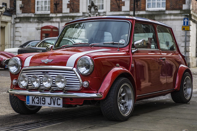
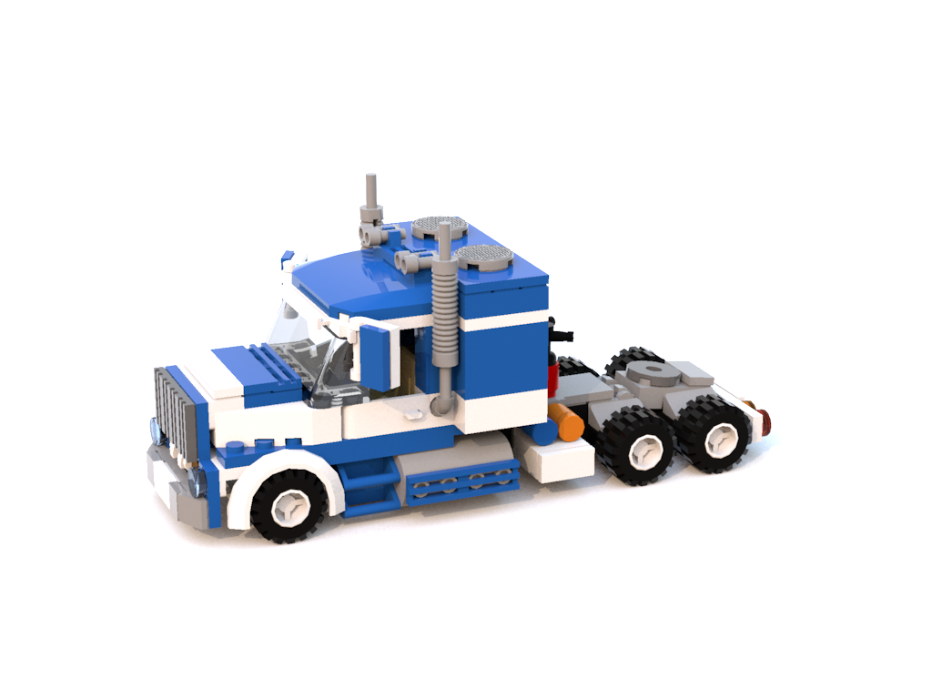
└── app_object_report_multi.R
├── README.Rmd
└── README.md
/apps.png:
--------------------------------------------------------------------------------
https://raw.githubusercontent.com/zappingseb/biowarptruck/HEAD/apps.png
--------------------------------------------------------------------------------
/example_packaged/graphics/car1.png:
--------------------------------------------------------------------------------
https://raw.githubusercontent.com/zappingseb/biowarptruck/HEAD/example_packaged/graphics/car1.png
--------------------------------------------------------------------------------
/example_packaged/graphics/pdf.png:
--------------------------------------------------------------------------------
https://raw.githubusercontent.com/zappingseb/biowarptruck/HEAD/example_packaged/graphics/pdf.png
--------------------------------------------------------------------------------
/example_packaged/graphics/image1.jpg:
--------------------------------------------------------------------------------
https://raw.githubusercontent.com/zappingseb/biowarptruck/HEAD/example_packaged/graphics/image1.jpg
--------------------------------------------------------------------------------
/example_packaged/graphics/images.pptx:
--------------------------------------------------------------------------------
https://raw.githubusercontent.com/zappingseb/biowarptruck/HEAD/example_packaged/graphics/images.pptx
--------------------------------------------------------------------------------
/example_packaged/graphics/fulltruck.png:
--------------------------------------------------------------------------------
https://raw.githubusercontent.com/zappingseb/biowarptruck/HEAD/example_packaged/graphics/fulltruck.png
--------------------------------------------------------------------------------
/example_packaged/graphics/constructor.png:
--------------------------------------------------------------------------------
https://raw.githubusercontent.com/zappingseb/biowarptruck/HEAD/example_packaged/graphics/constructor.png
--------------------------------------------------------------------------------
/example_packaged/graphics/class_diagram.png:
--------------------------------------------------------------------------------
https://raw.githubusercontent.com/zappingseb/biowarptruck/HEAD/example_packaged/graphics/class_diagram.png
--------------------------------------------------------------------------------
/example_packaged/graphics/construction_plan.png:
--------------------------------------------------------------------------------
https://raw.githubusercontent.com/zappingseb/biowarptruck/HEAD/example_packaged/graphics/construction_plan.png
--------------------------------------------------------------------------------
/example_packaged/graphics/class_diagram_core.png:
--------------------------------------------------------------------------------
https://raw.githubusercontent.com/zappingseb/biowarptruck/HEAD/example_packaged/graphics/class_diagram_core.png
--------------------------------------------------------------------------------
/example_packaged/graphics/construction_plan_done.png:
--------------------------------------------------------------------------------
https://raw.githubusercontent.com/zappingseb/biowarptruck/HEAD/example_packaged/graphics/construction_plan_done.png
--------------------------------------------------------------------------------
/biowarptruck.Rproj:
--------------------------------------------------------------------------------
1 | Version: 1.0
2 |
3 | RestoreWorkspace: Default
4 | SaveWorkspace: Default
5 | AlwaysSaveHistory: Default
6 |
7 | EnableCodeIndexing: Yes
8 | UseSpacesForTab: Yes
9 | NumSpacesForTab: 2
10 | Encoding: UTF-8
11 |
12 | RnwWeave: Sweave
13 | LaTeX: pdfLaTeX
14 |
--------------------------------------------------------------------------------
/example_packaged/config.xml:
--------------------------------------------------------------------------------
1 |
2 |
3 |
4 | module1
5 | Plot Module
6 | module1
7 | PlotReport
8 |
9 |
10 | module2
11 | Text Output
12 | module2
13 | TableReport
14 |
15 |
16 |
17 |
--------------------------------------------------------------------------------
/example_packaged/module1/DESCRIPTION:
--------------------------------------------------------------------------------
1 | Package: module1
2 | Version: 1.0.0
3 | Date: 2018-08-22
4 | Title: A package defining which a plot module App
5 | Authors@R: c(
6 | person("Sebastian", "Wolf", , "zappingseb@gmail.com", role = c("aut","cre"))
7 | )
8 | Depends:
9 | R (>= 3.1.3),
10 | appCore
11 | Description: This package provides some functionality to create plots for
12 | one observation
13 | Collate:
14 | module1.R
15 | VignetteBuilder: knitr
16 | License: GPL (>= 2)
17 | RoxygenNote: 6.0.1
18 |
--------------------------------------------------------------------------------
/example_packaged/module2/DESCRIPTION:
--------------------------------------------------------------------------------
1 | Package: module2
2 | Version: 1.0.0
3 | Date: 2018-08-22
4 | Title: A package defining which a text output module App
5 | Authors@R: c(
6 | person("Sebastian", "Wolf", , "zappingseb@gmail.com", role = c("aut","cre"))
7 | )
8 | Depends:
9 | R (>= 3.1.3),
10 | appCore,
11 | gridExtra
12 | Description: This package provides some functionality to create a table for
13 | one observation
14 | Collate:
15 | module2.R
16 | VignetteBuilder: knitr
17 | License: GPL (>= 2)
18 | RoxygenNote: 6.0.1
19 |
--------------------------------------------------------------------------------
/example_packaged/README.md:
--------------------------------------------------------------------------------
1 | to run this you need to:
2 |
3 | ```
4 | install.packages(c("devtools","rlang","XML","methods","gridExtra"))
5 | ```
6 |
7 | Afterwards start the app by
8 |
9 | ```
10 | shiny::runApp('example_packaged')
11 | ```
12 |
13 | ---
14 |
15 |
16 | The app is described inside this
17 |
18 | [Medium Article](https://medium.com/p/c977015bc6a9?source=your_stories_page---------------------------)
19 |
20 | ---
21 |
22 | **In any case of trouble do not hesitate to contact me**
23 |
24 | http://linkedin.com/in/zappingseb
25 |
26 | or
27 |
28 | https://github.com/zappingseb
29 |
--------------------------------------------------------------------------------
/example_apps/app_stiff.R:
--------------------------------------------------------------------------------
1 | server <- function(input, output) {
2 | # Output Gray Histogram
3 | output$distPlot <- renderPlot({
4 | x = sample(x = seq(from=0,to=100,by=0.1), size=input$obs,replace=T)
5 | plot(
6 | x = x,
7 | x+sample(x = 0.1:4, size=input$obs,replace=T)*sample(x = c(-1,1), size=input$obs,replace=T)
8 | )
9 | })
10 |
11 | }
12 |
13 | # Simple shiny App containing the standard histogram + PDF render and Download button
14 | ui <- fluidPage(
15 | sidebarLayout(
16 | sidebarPanel(
17 | sliderInput(
18 | "obs",
19 | "Number of observations:", min = 10, max = 500, value = 100)
20 | ),
21 | mainPanel(
22 | plotOutput("distPlot")
23 | )
24 | )
25 | )
26 | shinyApp(ui = ui, server = server)
27 |
--------------------------------------------------------------------------------
/example_packaged/core/DESCRIPTION:
--------------------------------------------------------------------------------
1 | Package: appCore
2 | Version: 1.0.0
3 | Date: 2018-08-22
4 | Title: A package defining which elements can appear inside an app
5 | Authors@R: c(
6 | person("Sebastian", "Wolf", , "zappingseb@gmail.com", role = c("aut","cre"))
7 | )
8 | Depends:
9 | R (>= 3.1.3),
10 | shiny,
11 | methods,
12 | rlang,
13 | XML,
14 | devtools
15 | Description: This provides a framework for R packages developed for
16 | a regulatory environment. It is based on the 'testthat' unit testing system and provides the adapter
17 | functionalities for XML-based test case definition as well as for standardized
18 | reporting of the test results.
19 | Collate:
20 | core.R
21 | VignetteBuilder: knitr
22 | License: GPL (>= 2)
23 | RoxygenNote: 6.0.1
24 |
--------------------------------------------------------------------------------
/example_apps/app_stiff_report.R:
--------------------------------------------------------------------------------
1 | server <- function(input, output) {
2 | # Output Gray Histogram
3 | output$distPlot <- renderPlot({
4 | hist(rnorm(input$obs), col = 'darkgray', border = 'white')
5 | })
6 | # Observe PDF button and create PDF
7 | observeEvent(input$"renderPDF",{
8 | pdf("test.pdf")
9 | hist(rnorm(input$obs), col = 'darkgray', border = 'white')
10 | dev.off()
11 | output$renderedPDF <- renderText("PDF rendered")
12 |
13 | })
14 |
15 | # Observe Download Button and return rendered PDF
16 | output$downloadPDF <- downloadHandler(
17 | filename = "test.pdf",
18 | content = function(file) {
19 | file.copy("test.pdf", file, overwrite = TRUE)
20 | }
21 | )
22 | }
23 |
24 | # Simple shiny App containing the standard histogram + PDF render and Download button
25 | ui <- fluidPage(
26 | sidebarLayout(
27 | sidebarPanel(
28 | sliderInput("obs", "Number of observations:", min = 10, max = 500, value = 100),
29 | actionButton("renderPDF","Render a Report"),
30 | textOutput("renderedPDF"),
31 | downloadButton("downloadPDF","Get rendered PDF")
32 | ),
33 | mainPanel(
34 | plotOutput("distPlot")
35 | )
36 | )
37 | )
38 | shinyApp(ui = ui, server = server)
39 |
--------------------------------------------------------------------------------
/example_packaged/module2/R/module2.R:
--------------------------------------------------------------------------------
1 |
2 | setClass("TableElement", representation(obs="numeric"), contains = "AnyPlot")
3 |
4 |
5 | # Define Children of Report class to enable different reports easily ---------------
6 | setClass("TableReport",contains = "Report")
7 |
8 |
9 |
10 |
11 | #' Construct the TableElement class
12 | #'
13 | #' The class constructed will contain a random data.frame with one
14 | #' column and 5 elements as its plot_element
15 | #'
16 | #' @param obs (\code{numeric}) How many observations to show in the histogram
17 | #'
18 | #' @return \code{TableElement} an object of class TableElement
19 | #'
20 | #' @author Sebastian Wolf (\email{zappingseb@@gmail.com})
21 | TableElement <- function(obs=100){
22 | new("TableElement",
23 | plot_element = expr(data.frame(x=sample(x=!!obs,size=5)))
24 | )
25 | }
26 |
27 |
28 | #' Constructor for a TableReport
29 | TableReport <- function(obs=100){
30 | new("TableReport",
31 | plots=list(
32 | TableElement(obs=obs)
33 | ),
34 | filename="test_text.pdf",
35 | obs=obs,
36 | rendered=F
37 | )
38 | }
39 |
40 |
41 | # Table Methods -------------------------------------------------------------
42 |
43 | setMethod("shinyElement",signature = "TableElement",definition = function(object){
44 | renderDataTable(evalElement(object))
45 | })
46 |
47 | #' Method to plot a Plot element
48 | setMethod("pdfElement",signature = "TableElement",definition = function(object){
49 | grid.table(evalElement(object))
50 | })
51 |
--------------------------------------------------------------------------------
/example_packaged/module1/R/module1.R:
--------------------------------------------------------------------------------
1 |
2 |
3 | # Define Classes to use inside the apps ------------------------------------------------------------
4 | setClass("HistPlot", representation(color="character",obs="numeric"), contains = "AnyPlot")
5 | setClass("ScatterPlot", representation(obs="numeric"), contains = "AnyPlot")
6 | setClass("PlotReport",contains = "Report")
7 |
8 |
9 | #' Construct the HistPlot class
10 | #'
11 | #' The class constructed will contain a Histogram as
12 | #' its plot element
13 | #'
14 | #' @param color (\code{character}) A color in which to show the bars of the plot
15 | #' @param obs (\code{numeric}) How many observations to show in the histogram
16 | #'
17 | #' @return \code{HistPlot} an object of class HistPlot
18 | #'
19 | #' @author Sebastian Wolf (\email{zappingseb@@gmail.com})
20 | HistPlot <- function(color="darkgrey",obs=100){
21 | new("HistPlot",
22 | plot_element = expr(hist(rnorm(!!obs), col = !!color, border = 'white')),
23 | color = color,
24 | obs = obs
25 | )
26 | }
27 |
28 | #' Construct the ScatterPlot class
29 | #'
30 | #' The class constructed will contain a random scatterplot as
31 | #' its plot element
32 | #'
33 | #' @param obs (\code{numeric}) How many observations to show in the histogram
34 | #'
35 | #' @return \code{ScatterPlot} an object of class ScatterPlot
36 | #'
37 | #' @author Sebastian Wolf (\email{zappingseb@@gmail.com})
38 | ScatterPlot <- function(obs=100){
39 | new("ScatterPlot",
40 | plot_element = expr(plot(sample(!!obs),sample(!!obs))),
41 | obs = obs
42 | )
43 | }
44 |
45 | #' Constructor of a PlotReport
46 | PlotReport <- function(obs=100){
47 | new("PlotReport",
48 | plots = list(
49 | HistPlot(color="darkgrey", obs=obs),
50 | ScatterPlot(obs=obs)
51 | ),
52 | filename="test_plots.pdf",
53 | obs=obs,
54 | rendered=FALSE
55 | )
56 | }
--------------------------------------------------------------------------------
/example_apps/app_object.R:
--------------------------------------------------------------------------------
1 | library(methods)
2 | library(rlang)
3 |
4 |
5 | setGeneric("plotElement",where = parent.frame(),def = function(object){standardGeneric("plotElement")})
6 | setGeneric("shinyElement",where = parent.frame(),def = function(object){standardGeneric("shinyElement")})
7 | setClass("AnyPlot", representation(plot_element = "call"))
8 | setClass("HistPlot", representation(color="character",obs="numeric"), contains = "AnyPlot")
9 |
10 | AnyPlot <- function(plot_element=expr(plot(1,1))){
11 | new("AnyPlot",
12 | plot_element = plot_element
13 | )
14 | }
15 |
16 | HistPlot <- function(color="darkgrey",obs=100){
17 | new("HistPlot",
18 | plot_element = expr(hist(rnorm(!!obs), col = !!color, border = 'white')),
19 | color = color,
20 | obs = obs
21 | )
22 | }
23 |
24 | #' Method to plot a Plot element
25 | setMethod("plotElement",signature = "AnyPlot",definition = function(object){
26 | eval(object@plot_element)
27 | })
28 | #' Method to render a Plot Element
29 | setMethod("shinyElement",signature = "AnyPlot",definition = function(object){
30 | renderPlot(plotElement(object))
31 | })
32 |
33 |
34 |
35 | server <- function(input, output, session) {
36 |
37 | # Create a reactive to create the Report object
38 | report_obj <- reactive(HistPlot(obs=input$obs))
39 |
40 | # Check for change of the slider to change the plots
41 | observeEvent(input$obs,{
42 | output$renderedPDF <- renderText("")
43 | output$renderPlot <- shinyElement( report_obj() )
44 | } )
45 |
46 | }
47 |
48 | # Simple shiny App containing the standard histogram + PDF render and Download button
49 | ui <- fluidPage(
50 | sidebarLayout(
51 | sidebarPanel(
52 | sliderInput("obs", "Number of observations:", min = 10, max = 500, value = 100)
53 | ),
54 | mainPanel(
55 | plotOutput("renderPlot")
56 | )
57 | )
58 | )
59 | shinyApp(ui = ui, server = server)
--------------------------------------------------------------------------------
/example_apps/app_stiff_report_multi.R:
--------------------------------------------------------------------------------
1 | server <- function(input, output) {
2 | # Output Gray Histogram
3 | output$distPlot <- renderPlot({
4 | write(paste0("hist(rnorm(",input$obs,"), col = 'darkgray', border = 'white') evaluated"),file="app.log",append=TRUE)
5 | hist(rnorm(input$obs), col = 'darkgray', border = 'white')
6 | })
7 | # Output Blue Histogram
8 | output$distPlot2 <- renderPlot({
9 | write(paste0("hist(rnorm(",input$obs,"), col = 'blue', border = 'white') evaluated"),file="app.log",append=TRUE)
10 | hist(rnorm(input$obs), col = 'blue', border = 'white')
11 | })
12 | # Output Blue Histogram
13 | output$scatterplot <- renderPlot({
14 | write(
15 | paste0("plot(sample(",input$obs,"), sample(",input$obs,") evaluated"),file="app.log",append=TRUE)
16 | plot(sample(input$obs), sample(input$obs))
17 | })
18 |
19 | # Observe PDF button and create PDF
20 | observeEvent(input$"renderPDF",{
21 | tryCatch({
22 | pdf("test.pdf")
23 | hist(rnorm(input$obs), col = 'blue', border = 'white')
24 | hist(rnorm(input$obs), col = 'darkgray', border = 'white')
25 | plot(sample(input$obs), sample(input$obs))
26 | dev.off()
27 | output$renderedPDF <- renderText("PDF rendered")
28 | },error=function(e){output$renderedPDF <- renderText("PDF could not be rendered")})
29 |
30 |
31 | })
32 |
33 | # Observe Download Button and return rendered PDF
34 | output$downloadPDF <- downloadHandler(
35 | filename = "test.pdf",
36 | content = function(file) {
37 | file.copy("test.pdf", file, overwrite = TRUE)
38 | }
39 | )
40 | }
41 |
42 | # Simple shiny App containing the standard histogram + PDF render and Download button
43 | ui <- fluidPage(
44 | sidebarLayout(
45 | sidebarPanel(
46 | sliderInput("obs", "Number of observations:", min = 10, max = 500, value = 100),
47 | actionButton("renderPDF","Render a Report"),
48 | textOutput("renderedPDF"),
49 | downloadButton("downloadPDF","Get rendered PDF")
50 | ),
51 | mainPanel(
52 | plotOutput("distPlot"),
53 | plotOutput("distPlot2"),
54 | plotOutput("scatterplot")
55 | )
56 | )
57 | )
58 | shinyApp(ui = ui, server = server)
59 |
--------------------------------------------------------------------------------
/example_apps/app_object_report.R:
--------------------------------------------------------------------------------
1 | library(methods)
2 | library(stringr)
3 | library(rlang)
4 | library(glue)
5 |
6 | setGeneric("plotElement",where = parent.frame(),def = function(object){standardGeneric("plotElement")})
7 | setGeneric("pdfElement",where = parent.frame(),def = function(object){standardGeneric("pdfElement")})
8 | setGeneric("shinyElement",where = parent.frame(),def = function(object){standardGeneric("shinyElement")})
9 |
10 | setClass("AnyPlot", representation(plot_element = "call"))
11 | setClass("HistPlot", representation(color="character",obs="numeric"), contains = "AnyPlot")
12 | setClass("Report",representation(plots="list",filename="character",obs="numeric",rendered="logical"))
13 |
14 | AnyPlot <- function(plot_element=expr(plot(1,1))){
15 | new("AnyPlot",
16 | plot_element = plot_element
17 | )
18 | }
19 |
20 | HistPlot <- function(color="darkgrey",obs=100){
21 | new("HistPlot",
22 | plot_element = expr(hist(rnorm(!!obs), col = !!color, border = 'white')),
23 | color = color,
24 | obs = obs
25 | )
26 | }
27 |
28 | #' Method to plot a Plot element
29 | setMethod("plotElement",signature = "AnyPlot",definition = function(object){
30 | eval(object@plot_element)
31 | })
32 | #' Method to render a Plot Element
33 | setMethod("shinyElement",signature = "AnyPlot",definition = function(object){
34 | renderPlot(plotElement(object))
35 | })
36 |
37 | #' Method to generate a PDF Report from a Report Element
38 | setMethod("pdfElement",signature = "AnyPlot",definition = function(object){
39 | pdf("test.pdf")
40 | plotElement(object)
41 | dev.off()
42 | })
43 |
44 |
45 | server <- function(input, output) {
46 |
47 | # Create a reactive to create the HistPlot object
48 | report_obj <- reactive(HistPlot(obs=input$obs))
49 |
50 | # Check for change of the slider to change the plots
51 | observeEvent(input$obs,{
52 | output$renderedPDF <- renderText("")
53 | output$reportReport <- shinyElement( report_obj() )
54 | } )
55 |
56 | # Observe PDF button and create PDF
57 | observeEvent(input$"renderPDF",{
58 | report <- pdfElement(report_obj())
59 | output$renderedPDF <- renderText("PDF rendered")
60 |
61 | })
62 |
63 | # Observe Download Button and return rendered PDF
64 | output$downloadPDF <- downloadHandler(
65 | filename = "test.pdf",
66 | content = function(file) {
67 | file.copy("test.pdf", file, overwrite = TRUE)
68 | }
69 | )
70 | }
71 |
72 | # Simple shiny App containing the standard histogram + PDF render and Download button
73 | ui <- fluidPage(
74 | sidebarLayout(
75 | sidebarPanel(
76 | sliderInput("obs", "Number of observations:", min = 10, max = 500, value = 100),
77 | actionButton("renderPDF","Render a Report"),
78 | textOutput("renderedPDF"),
79 | downloadButton("downloadPDF","Get rendered PDF")
80 | ),
81 | mainPanel(
82 | plotOutput("reportReport")
83 | )
84 | )
85 | )
86 | shinyApp(ui = ui, server = server)
--------------------------------------------------------------------------------
/example_packaged/app.R:
--------------------------------------------------------------------------------
1 | library(devtools)
2 |
3 | # Derive the core package to have all basics inside
4 | devtools::load_all("./core")
5 |
6 | #- Read the plan functions --------------------------
7 |
8 | #' Load an app Module Package
9 | #' @param xmlItem (\code{xmlNode})
10 | #' @export
11 | #'
12 | #' @author Sebastian Wolf (\email{zappingseb@@gmail.com})
13 | #'
14 | load_module <- function(xmlItem){
15 | # Load the desired module package
16 | devtools::load_all(paste0("./",xmlValue(xmlItem[["package"]])))
17 | }
18 |
19 | #' Create a TabPanel from an XMLItem
20 | #'
21 | #' @param xmlItem (\code{xmlNode})
22 | #'
23 | #' @export
24 | #'
25 | #' @author Sebastian Wolf (\email{zappingseb@@gmail.com})
26 | #'
27 | module_tab <- function(xmlItem){
28 | # Return a shiny tabPanel for the package
29 | tabPanel(xmlValue(xmlItem[["name"]]),
30 | uiOutput(xmlValue(xmlItem[["id"]]))
31 | )
32 | }
33 |
34 | server <- function(input,output){
35 |
36 | # Derive the infos from the configuration and store it inside a list
37 | configuration <- xmlApply(xmlRoot(xmlParse("config.xml")),function(xmlItem){
38 | load_module(xmlItem)
39 |
40 | # Append Tabs to the Reporting Window
41 | appendTab("modules",module_tab(xmlItem),select = TRUE)
42 |
43 | list(
44 | name = xmlValue(xmlItem[["name"]]),
45 | class = xmlValue(xmlItem[["class"]]),
46 | id = xmlValue(xmlItem[["id"]])
47 | )
48 | })
49 |
50 |
51 | # Create a reactive to create the Report object due to
52 | # the chosen module
53 | report_obj <- reactive({
54 | module <- unlist(lapply(configuration,function(x)x$name==input$modules))
55 | if(!any(module))module <- c(TRUE,FALSE)
56 | do.call(configuration[[which(module)]][["class"]],
57 | args=list(
58 | obs = input$obs
59 | ))
60 | })
61 |
62 | # Check for change of the slider/tab to re-calculate the report modules
63 | observeEvent({input$obs
64 | input$modules},{
65 |
66 | # Clear all produced outputs
67 | output$renderedPDF <- renderText("")
68 | file.remove(list.files(pattern=".pdf"))
69 |
70 | # Derive chosen tab
71 | module <- unlist(lapply(configuration,function(x)x$name==input$modules))
72 | if(!any(module))module <- c(TRUE,FALSE)
73 |
74 | # Re-render the output of the chosen tab
75 | output[[configuration[[which(module)]][["id"]]]] <- shinyElement( report_obj() )
76 | })
77 |
78 | # Observe PDF button and create PDF
79 | observeEvent(input$"renderPDF",{
80 |
81 | # Create PDF
82 | report <- pdfElement(report_obj())
83 |
84 | # If the PDF was successfully rendered update text message
85 | if(report@rendered){
86 | output$renderedPDF <- renderText("PDF rendered")
87 | }else{
88 | output$renderedPDF <- renderText("PDF could not be rendered")
89 | }
90 | })
91 |
92 | # Observe Download Button and return rendered PDF
93 | output$downloadPDF <-
94 | downloadHandler(
95 | filename = report_obj()@filename,
96 | content = function(file) {
97 | file.copy( report_obj()@filename, file, overwrite = TRUE)
98 | }
99 | )
100 | }
101 |
102 | # Simple shiny App containing the standard histogram + PDF render and Download button
103 | ui <- fluidPage(
104 | sidebarLayout(
105 | sidebarPanel(
106 | sliderInput("obs", "Number of observations:", min = 10, max = 500, value = 100),
107 | actionButton("renderPDF","Render a Report"),
108 | textOutput("renderedPDF"),
109 | downloadButton("downloadPDF","Get rendered PDF")
110 | ),
111 | mainPanel(
112 | tabsetPanel(id='modules')
113 | )#mainPanel
114 | )#sidebarlayout
115 | )#fluidPage
116 |
117 |
118 | shinyApp(ui = ui, server = server)
--------------------------------------------------------------------------------
/example_apps/app_object_report_multi.R:
--------------------------------------------------------------------------------
1 | library(methods)
2 | library(stringr)
3 | library(rlang)
4 | library(glue)
5 |
6 | setGeneric("plotElement",where = parent.frame(),def = function(object){standardGeneric("plotElement")})
7 | setGeneric("pdfElement",where = parent.frame(),def = function(object){standardGeneric("pdfElement")})
8 | setGeneric("shinyElement",where = parent.frame(),def = function(object){standardGeneric("shinyElement")})
9 | setGeneric("logElement",where = parent.frame(),def = function(object){standardGeneric("logElement")})
10 |
11 | setClass("AnyPlot", representation(plot_element = "call"))
12 | setClass("HistPlot", representation(color="character",obs="numeric"), contains = "AnyPlot")
13 | setClass("ScatterPlot", representation(obs="numeric"), contains = "AnyPlot")
14 | setClass("Report",representation(plots="list",filename="character",obs="numeric",rendered="logical"))
15 |
16 | AnyPlot <- function(plot_element=expr(plot(1,1))){
17 | new("AnyPlot",
18 | plot_element = plot_element
19 | )
20 | }
21 |
22 | HistPlot <- function(color="darkgrey",obs=100){
23 | new("HistPlot",
24 | plot_element = expr(hist(rnorm(!!obs), col = !!color, border = 'white')),
25 | color = color,
26 | obs = obs
27 | )
28 | }
29 | ScatterPlot <- function(obs=100){
30 | new("ScatterPlot",
31 | plot_element = expr(plot(sample(!!obs),sample(!!obs))),
32 | obs = obs
33 | )
34 | }
35 |
36 | Report <- function(obs=100){
37 | new("Report",
38 | plots = list(
39 | HistPlot(color="darkgrey", obs=obs),
40 | HistPlot(color="blue", obs=obs),
41 | ScatterPlot(obs=obs)
42 | ),
43 | filename="test.pdf",
44 | obs=obs,
45 | rendered=FALSE
46 | )
47 | }
48 |
49 |
50 | #' Method to log a Plot Element
51 | setMethod("logElement",signature = "AnyPlot",definition = function(object){
52 | # print(deparse(object@plot_element))
53 | write(paste0(deparse(object@plot_element)," evaluated"),file="app.log",append=TRUE)
54 | })
55 | #' Method to plot a Plot element
56 | setMethod("plotElement",signature = "AnyPlot",definition = function(object){
57 | eval(object@plot_element)
58 | })
59 | #' Method to render a Plot Element
60 | setMethod("shinyElement",signature = "AnyPlot",definition = function(object){
61 | renderPlot(plotElement(object))
62 | })
63 |
64 | #' Method to generate a PDF Report from a Report Element
65 | setMethod("pdfElement",signature = "Report",definition = function(object){
66 | tryCatch({
67 | pdf(object@filename)
68 | lapply(object@plots,function(x){
69 | plotElement(x)
70 | })
71 | dev.off()
72 | object@rendered <- TRUE
73 | },error=function(e){warning("plot not rendered")#do nothing
74 | })
75 | return(object)
76 | })
77 |
78 | #' Tell how to generate the shiny Element for a report
79 | setMethod("shinyElement",signature = "Report",definition = function(object){
80 | renderUI({
81 | lapply(object@plots,
82 | function(x){
83 | logElement(x)
84 | shinyElement(x)
85 | })
86 | })
87 | })
88 |
89 |
90 | server <- function(input, output, session) {
91 |
92 | # Create a reactive to create the Report object
93 | report_obj <- reactive(Report(obs=input$obs))
94 |
95 | # Check for change of the slider to change the plots
96 | observeEvent(input$obs,{
97 | output$renderedPDF <- renderText("")
98 | output$reportReport <- shinyElement( report_obj() )
99 | } )
100 |
101 | # Observe PDF button and create PDF
102 | observeEvent(input$"renderPDF",{
103 | report <- pdfElement(report_obj())
104 | if(report@rendered){
105 | output$renderedPDF <- renderText("PDF rendered")
106 | }else{
107 | output$renderedPDF <- renderText("PDF could not be rendered")
108 | }
109 | })
110 |
111 | # Observe Download Button and return rendered PDF
112 | output$downloadPDF <- downloadHandler(
113 | filename = report_obj()@filename,
114 | content = function(file) {
115 | file.copy(report_obj()@filename, file, overwrite = TRUE)
116 | }
117 | )
118 | }
119 |
120 | # Simple shiny App containing the standard histogram + PDF render and Download button
121 | ui <- fluidPage(
122 | sidebarLayout(
123 | sidebarPanel(
124 | sliderInput("obs", "Number of observations:", min = 10, max = 500, value = 100),
125 | actionButton("renderPDF","Render a Report"),
126 | textOutput("renderedPDF"),
127 | downloadButton("downloadPDF","Get rendered PDF")
128 | ),
129 | mainPanel(
130 | uiOutput("reportReport")
131 | )
132 | )
133 | )
134 | shinyApp(ui = ui, server = server)
--------------------------------------------------------------------------------
/example_packaged/core/R/core.R:
--------------------------------------------------------------------------------
1 | # Define Generics ---------------------------------------------------------------------------------
2 | setGeneric("evalElement",def = function(object){standardGeneric("evalElement")})
3 | setGeneric("pdfElement",def = function(object){standardGeneric("pdfElement")})
4 | setGeneric("shinyElement",def = function(object){standardGeneric("shinyElement")})
5 | setGeneric("logElement",def = function(object){standardGeneric("logElement")})
6 |
7 | # Define Report and Plot Classes --------------------------------------------------------------------
8 |
9 |
10 | #' Report Module for apps
11 | #'
12 | #' @slot plots (\code{list}) A list of \link{AnyPlot} objects
13 | #' @slot filename (\code{character}) The name of the PDF to output
14 | #' @slot obs (\code{numeric}) The number of observations to be used to generate the report
15 | #' @slot rendered (\code{logical}) Whether the PDF was rendered or not
16 | #'
17 | #' @export
18 | #' @author Sebastian Wolf (\email{zappingseb@@gmail.com})
19 | setClass("Report",
20 | representation(
21 | plots="list",
22 | filename="character",
23 | obs="numeric",
24 | rendered="logical"))
25 |
26 | # Report Methods ------------------------------------------------------------
27 |
28 | #' Method to generate a PDF Report from a Report Element
29 | #'
30 | #' This function generates a PDF with all elements of the report
31 | #' and stores it on the drive. The PDF will have the name of the
32 | #' \code{filename} slot of the object.
33 | #'
34 | #' @param object \code{Report} An object
35 | #'
36 | #' @return object \code{Report} with a changed \code{rendered} slot
37 | #' @export
38 | #' @author Sebastian Wolf (\email{zappingseb@@gmail.com})
39 | setMethod("pdfElement",signature = "Report",definition = function(object){
40 | tryCatch({
41 | pdf(object@filename)
42 | lapply(object@plots,function(x){
43 | pdfElement(x)
44 | })
45 | dev.off()
46 | object@rendered <- TRUE
47 | },error=function(e){warning("plot not rendered")#do nothing
48 | })
49 | return(object)
50 | })
51 |
52 | #' Method to generate the shiny Element for a Report
53 | #'
54 | #' Log the call of each object inside the \code{plots} slot and additionally render
55 | #' it into the shiny output
56 | #'
57 | #' @param object \code{Report} An object
58 | #'
59 | #' @return The output of a \link[shiny]{renderUI} output of shiny
60 | #'
61 | #' @author Sebastian Wolf (\email{zappingseb@@gmail.com})
62 | #' @export
63 | setMethod("shinyElement",signature = "Report",definition = function(object){
64 | renderUI({
65 | lapply(object@plots,
66 | function(x){
67 | logElement(x)
68 | shinyElement(x)
69 | })
70 | })
71 | })
72 |
73 | #- Anyplot class ----------------------------------------------------------------
74 |
75 | #' Plot Module for apps
76 | #'
77 | #' @slot plot_element (\code{call}) A call that can upon \code{eval} return a plot element
78 | #'
79 | #' @export
80 | #' @author Sebastian Wolf (\email{zappingseb@@gmail.com})
81 | setClass("AnyPlot", representation(plot_element="call"))
82 |
83 |
84 | # Constructors of AnyPlot classes ---------------------------------------------------------------------------
85 |
86 | #' Construct the AnyPlot class
87 | #' @param plot_element (\code{call}) A call returning a plot
88 | #' @export
89 | #' @return \code{AnyPlot} an object of class AnyPlot
90 | #' @author Sebastian Wolf (\email{zappingseb@@gmail.com})
91 | AnyPlot <- function(plot_element=expr(plot(1,1))){
92 | new("AnyPlot",
93 | plot_element = plot_element
94 | )
95 | }
96 |
97 | # Plot Methods ------------------------------------------------------------
98 |
99 | #' Method to log a Plot Element
100 | #'
101 | #' @param object \code{AnyPlot} An object
102 | #'
103 | #' @return nothing is returned, the call of the object is written into a logfile
104 | #' @export
105 | #' @author Sebastian Wolf (\email{zappingseb@@gmail.com})
106 | setMethod("logElement",signature = "AnyPlot",definition = function(object){
107 | write(paste0(deparse(object@plot_element)," evaluated"), file="app.log",append=TRUE)
108 | })
109 |
110 | #' Method to plot a Plot element
111 | #'
112 | #' @param object \code{AnyPlot} An object
113 | #'
114 | #' @return A plot object, fully rendered
115 | #' @export
116 | #' @author Sebastian Wolf (\email{zappingseb@@gmail.com})
117 | setMethod("evalElement",signature = "AnyPlot",definition = function(object){
118 | eval(object@plot_element)
119 | })
120 | #' Method to return a PDF element
121 | #' @param object \code{AnyPlot} An object
122 | #'
123 | #' @return Same call as \link{evalElement}
124 | #' @export
125 | #' @author Sebastian Wolf (\email{zappingseb@@gmail.com})
126 | setMethod("pdfElement",signature = "AnyPlot",definition = function(object){
127 | evalElement(object)
128 | })
129 |
130 | #' Method to shiny output a Plot
131 | #'
132 | #' @param object \code{AnyPlot} An object
133 | #'
134 | #' @return A Shiny element created by \link[shiny]{renderPlot}
135 | #'
136 | #' @author Sebastian Wolf (\email{zappingseb@@gmail.com})
137 | #' @export
138 | setMethod("shinyElement",signature = "AnyPlot",definition = function(object){
139 | renderPlot(evalElement(object))
140 | })
141 |
142 |
--------------------------------------------------------------------------------
/README.Rmd:
--------------------------------------------------------------------------------
1 | ---
2 | title: How to Build a Shiny "Truck"!
3 | author: Sebastian Wolf
4 | date: '2018-08-28'
5 | slug: how-to-build-shiny-trucks-not-shiny-cars
6 | categories:
7 | - R Language
8 | - Shiny
9 | tags:
10 | - R Language
11 | - Shiny
12 | summary: ''
13 | draft: yes
14 | output: md_document
15 | ---
16 |
17 | ```{r setup, include = FALSE}
18 | # packages required for this post
19 | for (pkg in c('methods', 'rlang'))
20 | if (!requireNamespace(pkg)) install.packages(pkg)
21 |
22 | knitr::opts_chunk$set(echo=TRUE)
23 | ```
24 |
25 |
26 | ## Why is this about trucks?
27 |
28 | Last month, at the [R/Pharma](https://www.rinpharma.com) conference that took place on the Harvard Campus, I presented bioWARP, a large [Shiny](https://shiny.rstudio.com/) application containing more than 500,000 lines of code. Although several other Shiny apps were presented at the conference, I noticed that none of them came close to being as big as bioWARP. And I asked myself, why?
29 |
30 | I concluded that most people just don't need to built them that big! So now, I would like to explain why we needed such a large app and how we went about building it.
31 |
32 |
33 |
34 |
35 | To give you an idea of the scale I am talking about an automotive methaphor might be useful. A typical Shiny app I see in my daily work has about 50 or even less interaction items. Let's imagine this as a car. With less than 50 interactions think of a small car like a mini cooper. Compared to these applications, with more than 500 interactions, bioWARP is a truck, maybe even a "monster" truck. So why do my customers want to drive trucks when everyone else is driving cars?
36 |
37 |
38 | Images by [Paul V](https://flic.kr/p/B4TwtZ) and [DaveR](https://flic.kr/p/q33yzD)
39 |
40 |
41 |

42 |
43 |
44 |
45 |
 210 |
211 | [Image by Barney Sharman](https://www.flickr.com/photos/157267479@N02/27368344058/in/photostream/)
212 |
213 | The modularization and packaging now enables fast testing. Why? Each package can be tested using basic [testthat](https://github.com/r-lib/testthat) functionalities. So first we tested our *core* application package, that allows adding building blocks. Afterwards we tested each single package on its own. Finally, the whole application is tested. Our truck is ready to roll. Upon updates, we do not have to test the whole truck again. If we want to have larger tires, we just update the tire package, but not the *core*-package or any other packages.
214 |
215 | ### Config files
216 |
217 | The truck is made of bricks, actually the same bricks we used to build the car. Just many more of them. Now the hard part is putting them all together and not losing track.
218 |
219 | We are dealing with many the different **Modules** that we were writing. Each
220 | **Module** comes in one package. The main issue we had was that we wanted all apps to be deeply tested. During development of course not all apps were tested right away, so we had to give them a tag (tested yes/no). Additionally some apps required help pages, others don't. Some apps came with example data sets, some don't. Some apps had a nice title in them already, for some it shall be easy to configure. For each **Module** we'll also have to source `js` and `css` files, which we allowed to be additionally added for each app. The folder where to source them shall be chosen by the app author. We wanted to provide as much flexibility as possible while keeping our standards for Lego bricks (Look&Feel, logging, plotting and reporting). A simple example for such an app can be found on [github](https://github.com/zappingseb/biowarptruck/tree/master/example_packaged).
221 |
222 | We came up with the idea of config `XML` files. So the XML file contains all the information needed to tell what needs to be set for each **Module**. An example XML is given below which you can see as the LEGO manual. These small configurations allow managing the apps. We also build an `XML` that allows the apps to use features of what we call *core*-package. This `XML` file is rather difficult to set up. But imagine it tells which Plot shall be logged, which input shall be used and which plots shall go into the PDF report. It allows fast development while sticking to standards.
223 |
224 |
225 |
227 |
210 |
211 | [Image by Barney Sharman](https://www.flickr.com/photos/157267479@N02/27368344058/in/photostream/)
212 |
213 | The modularization and packaging now enables fast testing. Why? Each package can be tested using basic [testthat](https://github.com/r-lib/testthat) functionalities. So first we tested our *core* application package, that allows adding building blocks. Afterwards we tested each single package on its own. Finally, the whole application is tested. Our truck is ready to roll. Upon updates, we do not have to test the whole truck again. If we want to have larger tires, we just update the tire package, but not the *core*-package or any other packages.
214 |
215 | ### Config files
216 |
217 | The truck is made of bricks, actually the same bricks we used to build the car. Just many more of them. Now the hard part is putting them all together and not losing track.
218 |
219 | We are dealing with many the different **Modules** that we were writing. Each
220 | **Module** comes in one package. The main issue we had was that we wanted all apps to be deeply tested. During development of course not all apps were tested right away, so we had to give them a tag (tested yes/no). Additionally some apps required help pages, others don't. Some apps came with example data sets, some don't. Some apps had a nice title in them already, for some it shall be easy to configure. For each **Module** we'll also have to source `js` and `css` files, which we allowed to be additionally added for each app. The folder where to source them shall be chosen by the app author. We wanted to provide as much flexibility as possible while keeping our standards for Lego bricks (Look&Feel, logging, plotting and reporting). A simple example for such an app can be found on [github](https://github.com/zappingseb/biowarptruck/tree/master/example_packaged).
221 |
222 | We came up with the idea of config `XML` files. So the XML file contains all the information needed to tell what needs to be set for each **Module**. An example XML is given below which you can see as the LEGO manual. These small configurations allow managing the apps. We also build an `XML` that allows the apps to use features of what we call *core*-package. This `XML` file is rather difficult to set up. But imagine it tells which Plot shall be logged, which input shall be used and which plots shall go into the PDF report. It allows fast development while sticking to standards.
223 |
224 |
225 |
227 |
228 | ```{XML}
229 |
230 | modulepackage1
231 | modulepackage1_Module
232 | Great BoxPlot Module
233 | GBM
234 | .
235 |
236 | help/index.html
237 |
238 | - help/about.html
239 |
240 |
241 |
242 |
243 |
244 |
245 | ```
246 |
247 |
263 |
264 |

265 |
266 |
267 |
 309 |
309 |
from LegoBrickinstructions.com
310 |
311 |
312 | modulepackage1
313 | modulepackage1_Module
314 | Great BoxPlot Module
315 | GBM
316 | .
317 |
318 | help/index.html
319 |
320 | - help/about.html
321 |
322 |
323 |
324 |
325 |
326 |
327 |
328 | Inside the config file you can clearly see that now the title of the app
329 | and the location of help pages, example data sets is given. Even the
330 | name of the class that describes the **Module** is given. This allows us
331 | to rapidly add modules to our main app environment.
332 |
333 | At the end our truck is made of many parts, that all increase its power
334 | and strength. As we now have around 16 modules in our real (in
335 | production) app and each has between 20 and 50 inputs, the truck has 500
336 | inputs. All which look similar and can be used to produced standardized
337 | PDF reports. The truck can even become a monster truck and thanks to the
338 | config files will still be easy to manage.
339 |
340 | My message to shiny.car and shiny.truck developers
341 | --------------------------------------------------
342 |
343 | 1. Please do not start building a car until you know how many parts it
344 | will have at the end. Always consider it might become a truck. At
345 | first, always define your requirements.
346 | 2. Use modularization! Use [shiny
347 | modules](https://shiny.rstudio.com/articles/modules.html) or
348 | inheritance provided by object orientation (
349 | [s4](http://adv-r.had.co.nz/S4.html) or
350 | [s6](https://cran.r-project.org/web/packages/R6/vignettes/Introduction.html)
351 | ). Both keep you from changing a lot of code on minor changes in
352 | requirements.
353 | 3. Use standardization! Try to have all your inputs and outputs as
354 | standardized as possible. If you use simple output bricks it’s easy
355 | to output them in your preferred format. Features like logging, PDF
356 | reporting or even testing will be way easier with standardized
357 | elements. Standardized inputs allow your users to be comfortable
358 | with new apps way faster.
359 | 4. Don’t build real trucks, build Lego trucks.
360 |
361 |
362 |
363 |
364 |
365 |
366 |
--------------------------------------------------------------------------------