├── LICENSE.txt
├── README.md
├── define_3D_domain.png
├── fluvial_meanderpy_example_map.png
├── fluvial_meanderpy_example_section.png
├── meanderpy
├── .gitignore
├── __init__.py
├── meanderpy.ipynb
└── meanderpy.py
├── meanderpy_logo.svg
├── meanderpy_sketch.png
├── meanderpy_strat_vs_morph.png
└── setup.py
/LICENSE.txt:
--------------------------------------------------------------------------------
1 | Apache License
2 | Version 2.0, January 2004
3 | http://www.apache.org/licenses/
4 |
5 | TERMS AND CONDITIONS FOR USE, REPRODUCTION, AND DISTRIBUTION
6 |
7 | 1. Definitions.
8 |
9 | "License" shall mean the terms and conditions for use, reproduction,
10 | and distribution as defined by Sections 1 through 9 of this document.
11 |
12 | "Licensor" shall mean the copyright owner or entity authorized by
13 | the copyright owner that is granting the License.
14 |
15 | "Legal Entity" shall mean the union of the acting entity and all
16 | other entities that control, are controlled by, or are under common
17 | control with that entity. For the purposes of this definition,
18 | "control" means (i) the power, direct or indirect, to cause the
19 | direction or management of such entity, whether by contract or
20 | otherwise, or (ii) ownership of fifty percent (50%) or more of the
21 | outstanding shares, or (iii) beneficial ownership of such entity.
22 |
23 | "You" (or "Your") shall mean an individual or Legal Entity
24 | exercising permissions granted by this License.
25 |
26 | "Source" form shall mean the preferred form for making modifications,
27 | including but not limited to software source code, documentation
28 | source, and configuration files.
29 |
30 | "Object" form shall mean any form resulting from mechanical
31 | transformation or translation of a Source form, including but
32 | not limited to compiled object code, generated documentation,
33 | and conversions to other media types.
34 |
35 | "Work" shall mean the work of authorship, whether in Source or
36 | Object form, made available under the License, as indicated by a
37 | copyright notice that is included in or attached to the work
38 | (an example is provided in the Appendix below).
39 |
40 | "Derivative Works" shall mean any work, whether in Source or Object
41 | form, that is based on (or derived from) the Work and for which the
42 | editorial revisions, annotations, elaborations, or other modifications
43 | represent, as a whole, an original work of authorship. For the purposes
44 | of this License, Derivative Works shall not include works that remain
45 | separable from, or merely link (or bind by name) to the interfaces of,
46 | the Work and Derivative Works thereof.
47 |
48 | "Contribution" shall mean any work of authorship, including
49 | the original version of the Work and any modifications or additions
50 | to that Work or Derivative Works thereof, that is intentionally
51 | submitted to Licensor for inclusion in the Work by the copyright owner
52 | or by an individual or Legal Entity authorized to submit on behalf of
53 | the copyright owner. For the purposes of this definition, "submitted"
54 | means any form of electronic, verbal, or written communication sent
55 | to the Licensor or its representatives, including but not limited to
56 | communication on electronic mailing lists, source code control systems,
57 | and issue tracking systems that are managed by, or on behalf of, the
58 | Licensor for the purpose of discussing and improving the Work, but
59 | excluding communication that is conspicuously marked or otherwise
60 | designated in writing by the copyright owner as "Not a Contribution."
61 |
62 | "Contributor" shall mean Licensor and any individual or Legal Entity
63 | on behalf of whom a Contribution has been received by Licensor and
64 | subsequently incorporated within the Work.
65 |
66 | 2. Grant of Copyright License. Subject to the terms and conditions of
67 | this License, each Contributor hereby grants to You a perpetual,
68 | worldwide, non-exclusive, no-charge, royalty-free, irrevocable
69 | copyright license to reproduce, prepare Derivative Works of,
70 | publicly display, publicly perform, sublicense, and distribute the
71 | Work and such Derivative Works in Source or Object form.
72 |
73 | 3. Grant of Patent License. Subject to the terms and conditions of
74 | this License, each Contributor hereby grants to You a perpetual,
75 | worldwide, non-exclusive, no-charge, royalty-free, irrevocable
76 | (except as stated in this section) patent license to make, have made,
77 | use, offer to sell, sell, import, and otherwise transfer the Work,
78 | where such license applies only to those patent claims licensable
79 | by such Contributor that are necessarily infringed by their
80 | Contribution(s) alone or by combination of their Contribution(s)
81 | with the Work to which such Contribution(s) was submitted. If You
82 | institute patent litigation against any entity (including a
83 | cross-claim or counterclaim in a lawsuit) alleging that the Work
84 | or a Contribution incorporated within the Work constitutes direct
85 | or contributory patent infringement, then any patent licenses
86 | granted to You under this License for that Work shall terminate
87 | as of the date such litigation is filed.
88 |
89 | 4. Redistribution. You may reproduce and distribute copies of the
90 | Work or Derivative Works thereof in any medium, with or without
91 | modifications, and in Source or Object form, provided that You
92 | meet the following conditions:
93 |
94 | (a) You must give any other recipients of the Work or
95 | Derivative Works a copy of this License; and
96 |
97 | (b) You must cause any modified files to carry prominent notices
98 | stating that You changed the files; and
99 |
100 | (c) You must retain, in the Source form of any Derivative Works
101 | that You distribute, all copyright, patent, trademark, and
102 | attribution notices from the Source form of the Work,
103 | excluding those notices that do not pertain to any part of
104 | the Derivative Works; and
105 |
106 | (d) If the Work includes a "NOTICE" text file as part of its
107 | distribution, then any Derivative Works that You distribute must
108 | include a readable copy of the attribution notices contained
109 | within such NOTICE file, excluding those notices that do not
110 | pertain to any part of the Derivative Works, in at least one
111 | of the following places: within a NOTICE text file distributed
112 | as part of the Derivative Works; within the Source form or
113 | documentation, if provided along with the Derivative Works; or,
114 | within a display generated by the Derivative Works, if and
115 | wherever such third-party notices normally appear. The contents
116 | of the NOTICE file are for informational purposes only and
117 | do not modify the License. You may add Your own attribution
118 | notices within Derivative Works that You distribute, alongside
119 | or as an addendum to the NOTICE text from the Work, provided
120 | that such additional attribution notices cannot be construed
121 | as modifying the License.
122 |
123 | You may add Your own copyright statement to Your modifications and
124 | may provide additional or different license terms and conditions
125 | for use, reproduction, or distribution of Your modifications, or
126 | for any such Derivative Works as a whole, provided Your use,
127 | reproduction, and distribution of the Work otherwise complies with
128 | the conditions stated in this License.
129 |
130 | 5. Submission of Contributions. Unless You explicitly state otherwise,
131 | any Contribution intentionally submitted for inclusion in the Work
132 | by You to the Licensor shall be under the terms and conditions of
133 | this License, without any additional terms or conditions.
134 | Notwithstanding the above, nothing herein shall supersede or modify
135 | the terms of any separate license agreement you may have executed
136 | with Licensor regarding such Contributions.
137 |
138 | 6. Trademarks. This License does not grant permission to use the trade
139 | names, trademarks, service marks, or product names of the Licensor,
140 | except as required for reasonable and customary use in describing the
141 | origin of the Work and reproducing the content of the NOTICE file.
142 |
143 | 7. Disclaimer of Warranty. Unless required by applicable law or
144 | agreed to in writing, Licensor provides the Work (and each
145 | Contributor provides its Contributions) on an "AS IS" BASIS,
146 | WITHOUT WARRANTIES OR CONDITIONS OF ANY KIND, either express or
147 | implied, including, without limitation, any warranties or conditions
148 | of TITLE, NON-INFRINGEMENT, MERCHANTABILITY, or FITNESS FOR A
149 | PARTICULAR PURPOSE. You are solely responsible for determining the
150 | appropriateness of using or redistributing the Work and assume any
151 | risks associated with Your exercise of permissions under this License.
152 |
153 | 8. Limitation of Liability. In no event and under no legal theory,
154 | whether in tort (including negligence), contract, or otherwise,
155 | unless required by applicable law (such as deliberate and grossly
156 | negligent acts) or agreed to in writing, shall any Contributor be
157 | liable to You for damages, including any direct, indirect, special,
158 | incidental, or consequential damages of any character arising as a
159 | result of this License or out of the use or inability to use the
160 | Work (including but not limited to damages for loss of goodwill,
161 | work stoppage, computer failure or malfunction, or any and all
162 | other commercial damages or losses), even if such Contributor
163 | has been advised of the possibility of such damages.
164 |
165 | 9. Accepting Warranty or Additional Liability. While redistributing
166 | the Work or Derivative Works thereof, You may choose to offer,
167 | and charge a fee for, acceptance of support, warranty, indemnity,
168 | or other liability obligations and/or rights consistent with this
169 | License. However, in accepting such obligations, You may act only
170 | on Your own behalf and on Your sole responsibility, not on behalf
171 | of any other Contributor, and only if You agree to indemnify,
172 | defend, and hold each Contributor harmless for any liability
173 | incurred by, or claims asserted against, such Contributor by reason
174 | of your accepting any such warranty or additional liability.
175 |
176 | END OF TERMS AND CONDITIONS
177 |
178 | APPENDIX: How to apply the Apache License to your work.
179 |
180 | To apply the Apache License to your work, attach the following
181 | boilerplate notice, with the fields enclosed by brackets "[]"
182 | replaced with your own identifying information. (Don't include
183 | the brackets!) The text should be enclosed in the appropriate
184 | comment syntax for the file format. We also recommend that a
185 | file or class name and description of purpose be included on the
186 | same "printed page" as the copyright notice for easier
187 | identification within third-party archives.
188 |
189 | Copyright [2018] [Zoltan Sylvester]
190 |
191 | Licensed under the Apache License, Version 2.0 (the "License");
192 | you may not use this file except in compliance with the License.
193 | You may obtain a copy of the License at
194 |
195 | http://www.apache.org/licenses/LICENSE-2.0
196 |
197 | Unless required by applicable law or agreed to in writing, software
198 | distributed under the License is distributed on an "AS IS" BASIS,
199 | WITHOUT WARRANTIES OR CONDITIONS OF ANY KIND, either express or implied.
200 | See the License for the specific language governing permissions and
201 | limitations under the License.
202 |
--------------------------------------------------------------------------------
/README.md:
--------------------------------------------------------------------------------
1 |  2 |
3 | ## Description
4 |
5 | 'meanderpy' is a Python module that implements a simple numerical model of meandering, the one described by Howard & Knutson in their 1984 paper ["Sufficient Conditions for River Meandering: A Simulation Approach"](https://agupubs.onlinelibrary.wiley.com/doi/abs/10.1029/WR020i011p01659). This is a kinematic model that is based on computing migration rate as the weighted sum of upstream curvatures; flow velocity does not enter the equation. Curvature is transformed into a 'nominal migration rate' through multiplication with a migration rate (or erodibility) constant; in the Howard & Knutson (1984) paper this is a nonlinear relationship based on field observations that suggested a complex link between curvature and migration rate. In the 'meanderpy' module we use a simple linear relationship between the nominal migration rate and curvature, as recent work using time-lapse satellite imagery suggests that high curvatures result in high migration rates ([Sylvester et al., 2019](https://doi.org/10.1130/G45608.1)).
6 |
7 | ## Installation
8 |
9 |
2 |
3 | ## Description
4 |
5 | 'meanderpy' is a Python module that implements a simple numerical model of meandering, the one described by Howard & Knutson in their 1984 paper ["Sufficient Conditions for River Meandering: A Simulation Approach"](https://agupubs.onlinelibrary.wiley.com/doi/abs/10.1029/WR020i011p01659). This is a kinematic model that is based on computing migration rate as the weighted sum of upstream curvatures; flow velocity does not enter the equation. Curvature is transformed into a 'nominal migration rate' through multiplication with a migration rate (or erodibility) constant; in the Howard & Knutson (1984) paper this is a nonlinear relationship based on field observations that suggested a complex link between curvature and migration rate. In the 'meanderpy' module we use a simple linear relationship between the nominal migration rate and curvature, as recent work using time-lapse satellite imagery suggests that high curvatures result in high migration rates ([Sylvester et al., 2019](https://doi.org/10.1130/G45608.1)).
6 |
7 | ## Installation
8 |
9 | pip install meanderpy
10 |
11 | ## Requirements
12 |
13 | - numpy
14 | - matplotlib
15 | - scipy
16 | - PIL
17 | - numba
18 | - scikit-image
19 | - tqdm
20 | - jupyter
21 |
22 | ## Usage
23 |
24 | 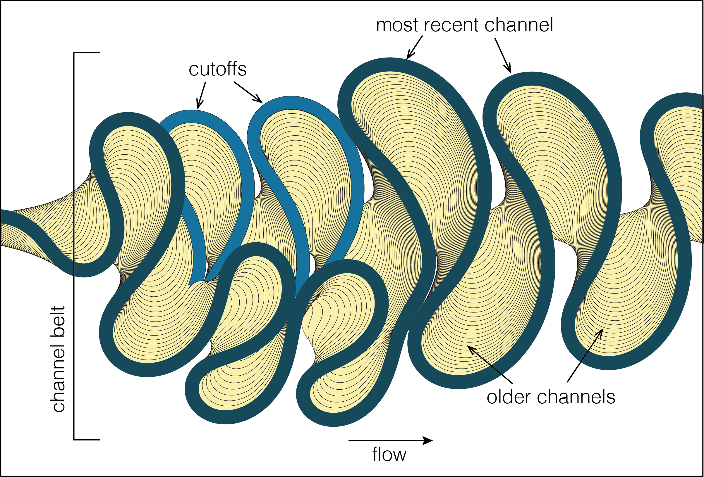 25 |
26 | The sketch above shows the three 'meanderpy' components: channel, cutoff, channel belt. These are implemented as classes; a 'Channel' and a 'Cutoff' are defined by their width, depth, and x,y,z centerline coordinates, and a 'ChannelBelt' is a collection of channels and cutoffs. In addition, the 'ChannelBelt' object also has a 'cl_times' and a 'cutoff_times' attribute that specify the age of the channels and the cutoffs. This age is relative to the start time of the simulation (= the first channel, age = 0.0).
27 |
28 | To run the below cells, you must first import the library:
29 |
30 | ```python
31 | import meanderpy as mp
32 | import numpy as np
33 | ```
34 |
35 | A reasonable set of input parameters are as follows:
36 |
37 | ```python
38 | nit = 1500 # number of iterations
39 | W = 200.0 # channel width (m)
40 | D = 6.0 # channel depth (m)
41 | depths = D * np.ones((nit,)) # channel depths for different iterations
42 | pad = 100 # padding (number of nodepoints along centerline)
43 | deltas = 50.0 # sampling distance along centerline
44 | Cfs = 0.011 * np.ones((nit,)) # dimensionless Chezy friction factor
45 | crdist = 2 * W # threshold distance at which cutoffs occur
46 | kl = 60.0/(365*24*60*60.0) # migration rate constant (m/s)
47 | kv = 1.0e-12 # vertical slope-dependent erosion rate constant (m/s)
48 | dt = 2*0.05*365*24*60*60.0 # time step (s)
49 | dens = 1000 # density of water (kg/m3)
50 | saved_ts = 20 # which time steps will be saved
51 | n_bends = 30 # approximate number of bends you want to model
52 | Sl = 0.0 # initial slope (matters more for submarine channels than rivers)
53 | t1 = 500 # time step when incision starts
54 | t2 = 700 # time step when lateral migration starts
55 | t3 = 1200 # time step when aggradation starts
56 | aggr_factor = 2e-9 # aggradation factor (m/s, about 0.18 m/year, it kicks in after t3)
57 | ```
58 |
59 | The initial Channel object can be created using the 'generate_initial_channel' function. This creates a straight line, with some noise added. However, a Channel can be created (and then used as the first channel in a ChannelBelt) using any set of x,y,z,W,D variables.
60 |
61 | ```python
62 | ch = mp.generate_initial_channel(W, depths[0], Sl, deltas, pad, n_bends) # initialize channel
63 | chb = mp.ChannelBelt(channels=[ch], cutoffs=[], cl_times=[0.0], cutoff_times=[]) # create channel belt object
64 | ```
65 |
66 | The core functionality of 'meanderpy' is built into the 'migrate' method of the 'ChannelBelt' class. This is the function that computes migration rates and moves the channel centerline to its new position. The last Channel of a ChannelBelt can be further migrated through applying the 'migrate' method to the ChannelBelt instance.
67 |
68 | ```python
69 | chb.migrate(nit,saved_ts,deltas,pad,crdist,depths,Cfs,kl,kv,dt,dens,t1,t2,t3,aggr_factor) # channel migration
70 | ```
71 |
72 | ChannelBelt objects can be visualized using the 'plot' method. This creates a map of all the channels and cutoffs in the channel belt; there are two styles of plotting: a 'stratigraphic' view and a 'morphologic' view (see below). The morphologic view tries to account for the fact that older point bars and oxbow lakes tend to be gradually covered with vegetation.
73 |
74 | ```python
75 | # migrate an additional 1000 iterations and plot results
76 | chb.migrate(1000,saved_ts,deltas,pad,crdist,depths,Cfs,kl,kv,dt,dens,t1,t2,t3,aggr_factor)
77 | fig = chb.plot('strat', 20, 60, chb.cl_times[-1], len(chb.channels)) # plotting
78 | ```
79 |
80 |
25 |
26 | The sketch above shows the three 'meanderpy' components: channel, cutoff, channel belt. These are implemented as classes; a 'Channel' and a 'Cutoff' are defined by their width, depth, and x,y,z centerline coordinates, and a 'ChannelBelt' is a collection of channels and cutoffs. In addition, the 'ChannelBelt' object also has a 'cl_times' and a 'cutoff_times' attribute that specify the age of the channels and the cutoffs. This age is relative to the start time of the simulation (= the first channel, age = 0.0).
27 |
28 | To run the below cells, you must first import the library:
29 |
30 | ```python
31 | import meanderpy as mp
32 | import numpy as np
33 | ```
34 |
35 | A reasonable set of input parameters are as follows:
36 |
37 | ```python
38 | nit = 1500 # number of iterations
39 | W = 200.0 # channel width (m)
40 | D = 6.0 # channel depth (m)
41 | depths = D * np.ones((nit,)) # channel depths for different iterations
42 | pad = 100 # padding (number of nodepoints along centerline)
43 | deltas = 50.0 # sampling distance along centerline
44 | Cfs = 0.011 * np.ones((nit,)) # dimensionless Chezy friction factor
45 | crdist = 2 * W # threshold distance at which cutoffs occur
46 | kl = 60.0/(365*24*60*60.0) # migration rate constant (m/s)
47 | kv = 1.0e-12 # vertical slope-dependent erosion rate constant (m/s)
48 | dt = 2*0.05*365*24*60*60.0 # time step (s)
49 | dens = 1000 # density of water (kg/m3)
50 | saved_ts = 20 # which time steps will be saved
51 | n_bends = 30 # approximate number of bends you want to model
52 | Sl = 0.0 # initial slope (matters more for submarine channels than rivers)
53 | t1 = 500 # time step when incision starts
54 | t2 = 700 # time step when lateral migration starts
55 | t3 = 1200 # time step when aggradation starts
56 | aggr_factor = 2e-9 # aggradation factor (m/s, about 0.18 m/year, it kicks in after t3)
57 | ```
58 |
59 | The initial Channel object can be created using the 'generate_initial_channel' function. This creates a straight line, with some noise added. However, a Channel can be created (and then used as the first channel in a ChannelBelt) using any set of x,y,z,W,D variables.
60 |
61 | ```python
62 | ch = mp.generate_initial_channel(W, depths[0], Sl, deltas, pad, n_bends) # initialize channel
63 | chb = mp.ChannelBelt(channels=[ch], cutoffs=[], cl_times=[0.0], cutoff_times=[]) # create channel belt object
64 | ```
65 |
66 | The core functionality of 'meanderpy' is built into the 'migrate' method of the 'ChannelBelt' class. This is the function that computes migration rates and moves the channel centerline to its new position. The last Channel of a ChannelBelt can be further migrated through applying the 'migrate' method to the ChannelBelt instance.
67 |
68 | ```python
69 | chb.migrate(nit,saved_ts,deltas,pad,crdist,depths,Cfs,kl,kv,dt,dens,t1,t2,t3,aggr_factor) # channel migration
70 | ```
71 |
72 | ChannelBelt objects can be visualized using the 'plot' method. This creates a map of all the channels and cutoffs in the channel belt; there are two styles of plotting: a 'stratigraphic' view and a 'morphologic' view (see below). The morphologic view tries to account for the fact that older point bars and oxbow lakes tend to be gradually covered with vegetation.
73 |
74 | ```python
75 | # migrate an additional 1000 iterations and plot results
76 | chb.migrate(1000,saved_ts,deltas,pad,crdist,depths,Cfs,kl,kv,dt,dens,t1,t2,t3,aggr_factor)
77 | fig = chb.plot('strat', 20, 60, chb.cl_times[-1], len(chb.channels)) # plotting
78 | ```
79 |
80 | 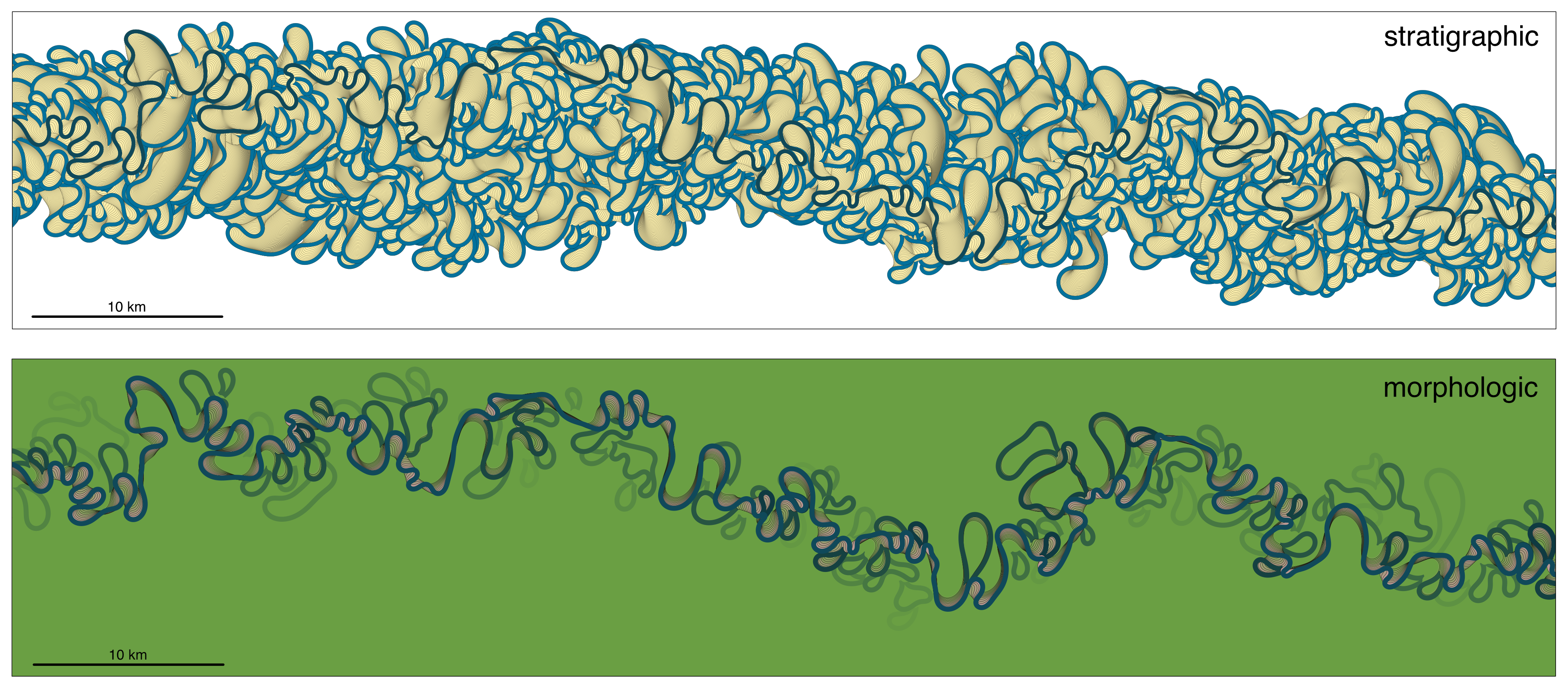 81 |
82 | A series of movie frames (in PNG format) can be created using the 'create_movie' method:
83 |
84 | ```python
85 | chb.create_movie(xmin,xmax,plot_type,filename,dirname,pb_age,ob_age,scale,end_time)
86 | ```
87 | The frames have to be assembled into an animation outside of 'meanderpy'.
88 |
89 | ## Build 3D model
90 |
91 | 'meanderpy' includes the functionality to build 3D stratigraphic models. However, this functionality is decoupled from the centerline generation, mainly because it would be computationally expensive to generate surfaces for all centerlines, along their whole lengths. Instead, the 3D model is only created after a Channelbelt object has been generated; a model domain is defined either through specifying the xmin, xmax, ymin, ymax coordinates, or through clicking the upper left and lower right corners of the domain, using the matplotlib 'ginput' command:
92 |
93 |
81 |
82 | A series of movie frames (in PNG format) can be created using the 'create_movie' method:
83 |
84 | ```python
85 | chb.create_movie(xmin,xmax,plot_type,filename,dirname,pb_age,ob_age,scale,end_time)
86 | ```
87 | The frames have to be assembled into an animation outside of 'meanderpy'.
88 |
89 | ## Build 3D model
90 |
91 | 'meanderpy' includes the functionality to build 3D stratigraphic models. However, this functionality is decoupled from the centerline generation, mainly because it would be computationally expensive to generate surfaces for all centerlines, along their whole lengths. Instead, the 3D model is only created after a Channelbelt object has been generated; a model domain is defined either through specifying the xmin, xmax, ymin, ymax coordinates, or through clicking the upper left and lower right corners of the domain, using the matplotlib 'ginput' command:
92 |
93 | 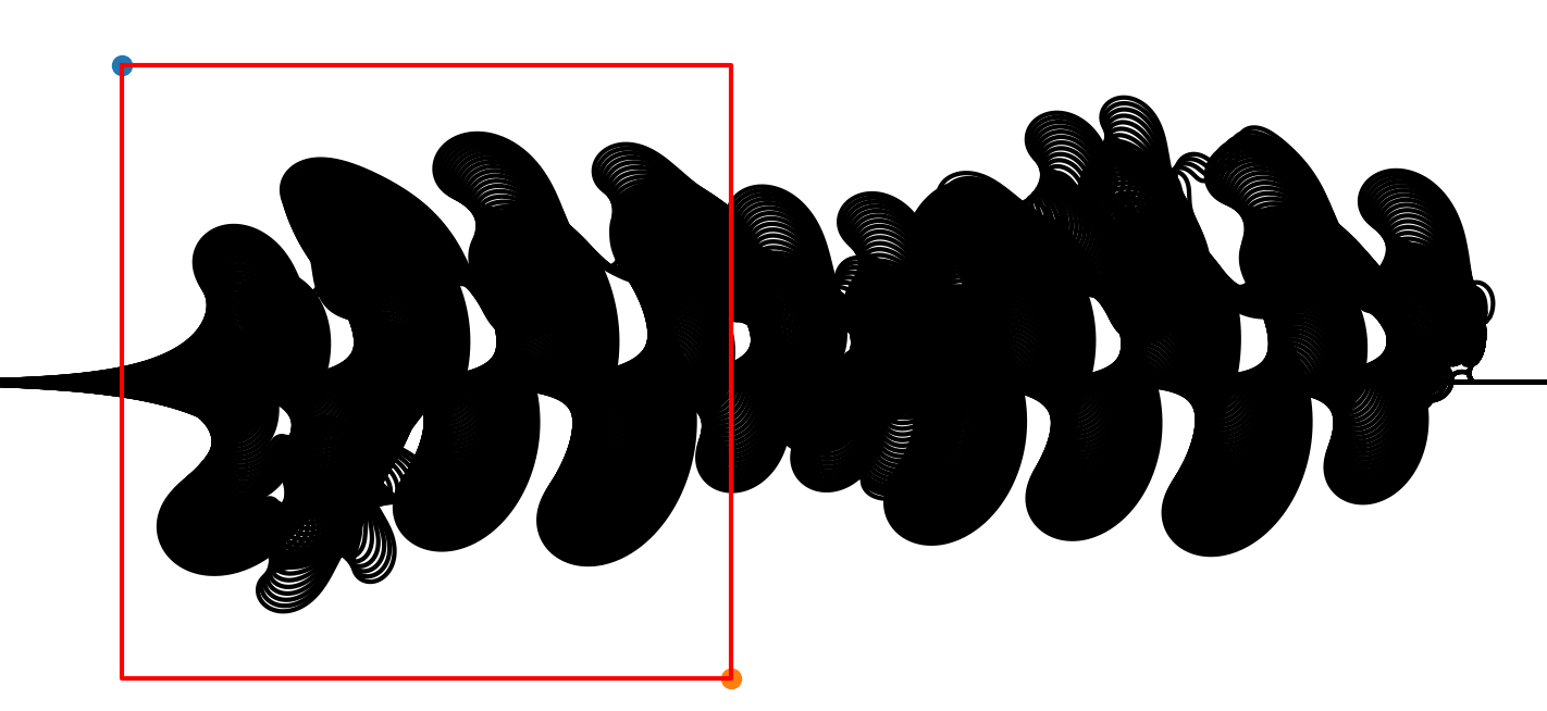 94 |
95 | Important parameters for a fluvial 3D model are the following:
96 |
97 | ```python
98 | Sl = 0.0 # initial slope (matters more for submarine channels than rivers)
99 | t1 = 500 # time step when incision starts
100 | t2 = 700 # time step when lateral migration starts
101 | t3 = 1400 # time step when aggradation starts
102 | aggr_factor = 4e-9 # aggradation rate (in m/s, it kicks in after t3)
103 | h_mud = 0.4 # thickness of overbank deposit for each time step
104 | dx = 10.0 # gridcell size in meters
105 | ```
106 | The first five of these parameters have to be specified before creating the centerlines. The initial slope (Sl) in a fluvial model is best set to zero, as typical gradients in meandering rivers are very low and artifacts associated with the along-channel slope variation will be visible in the model surfaces [this is not an issue with steeper submarine channel models]. t1 is the time step when incision starts; before t1, the centerlines are given time to develop some sinuosity. At time t2, incision stops and the channel only migrates laterally until t3; this is the time when aggradation starts. The rate of incision (if Sl is set to zero) is set by the quantity 'kv x dens x 9.81 x D x dt x 0.01' (as if the slope was 0.01, but of course it is not), where kv is the vertical incision rate constant. This approach does not require a new incision rate constant. The rate of aggradation is set by 'aggr_factor x dt' (so 'aggr_factor' must be a small number, as it is measured in m/s). 'h_mud' is the maximum thickness of the overbank deposit in each time step, and 'dx' is the gridcell size in meters. 'h_mud' has to be large enough that it matches the channel aggradation rate; weird artefacts are generated otherwise.
107 |
108 | The Jupyter notebook has two examples for building 3D models, for a fluvial and a submarine channel system. The 'plot_xsection' method can be used to create a cross section at a given x (pixel) coordinate (this is the first argument of the function). The second argument determines the colors that are used for the different facies (in this case: brown, yellow, brown RGB values). The third argument is the vertical exaggeration.
109 |
110 | ```python
111 | fig1,fig2,fig3 = chb_3d.plot_xsection(343, [[0.5,0.25,0],[0.9,0.9,0],[0.5,0.25,0]], 4)
112 | ```
113 | This function also plots the basal erosional surface and the final topographic surface. An example topographic surface and a zoomed-in cross section are shown below.
114 |
115 |
94 |
95 | Important parameters for a fluvial 3D model are the following:
96 |
97 | ```python
98 | Sl = 0.0 # initial slope (matters more for submarine channels than rivers)
99 | t1 = 500 # time step when incision starts
100 | t2 = 700 # time step when lateral migration starts
101 | t3 = 1400 # time step when aggradation starts
102 | aggr_factor = 4e-9 # aggradation rate (in m/s, it kicks in after t3)
103 | h_mud = 0.4 # thickness of overbank deposit for each time step
104 | dx = 10.0 # gridcell size in meters
105 | ```
106 | The first five of these parameters have to be specified before creating the centerlines. The initial slope (Sl) in a fluvial model is best set to zero, as typical gradients in meandering rivers are very low and artifacts associated with the along-channel slope variation will be visible in the model surfaces [this is not an issue with steeper submarine channel models]. t1 is the time step when incision starts; before t1, the centerlines are given time to develop some sinuosity. At time t2, incision stops and the channel only migrates laterally until t3; this is the time when aggradation starts. The rate of incision (if Sl is set to zero) is set by the quantity 'kv x dens x 9.81 x D x dt x 0.01' (as if the slope was 0.01, but of course it is not), where kv is the vertical incision rate constant. This approach does not require a new incision rate constant. The rate of aggradation is set by 'aggr_factor x dt' (so 'aggr_factor' must be a small number, as it is measured in m/s). 'h_mud' is the maximum thickness of the overbank deposit in each time step, and 'dx' is the gridcell size in meters. 'h_mud' has to be large enough that it matches the channel aggradation rate; weird artefacts are generated otherwise.
107 |
108 | The Jupyter notebook has two examples for building 3D models, for a fluvial and a submarine channel system. The 'plot_xsection' method can be used to create a cross section at a given x (pixel) coordinate (this is the first argument of the function). The second argument determines the colors that are used for the different facies (in this case: brown, yellow, brown RGB values). The third argument is the vertical exaggeration.
109 |
110 | ```python
111 | fig1,fig2,fig3 = chb_3d.plot_xsection(343, [[0.5,0.25,0],[0.9,0.9,0],[0.5,0.25,0]], 4)
112 | ```
113 | This function also plots the basal erosional surface and the final topographic surface. An example topographic surface and a zoomed-in cross section are shown below.
114 |
115 | 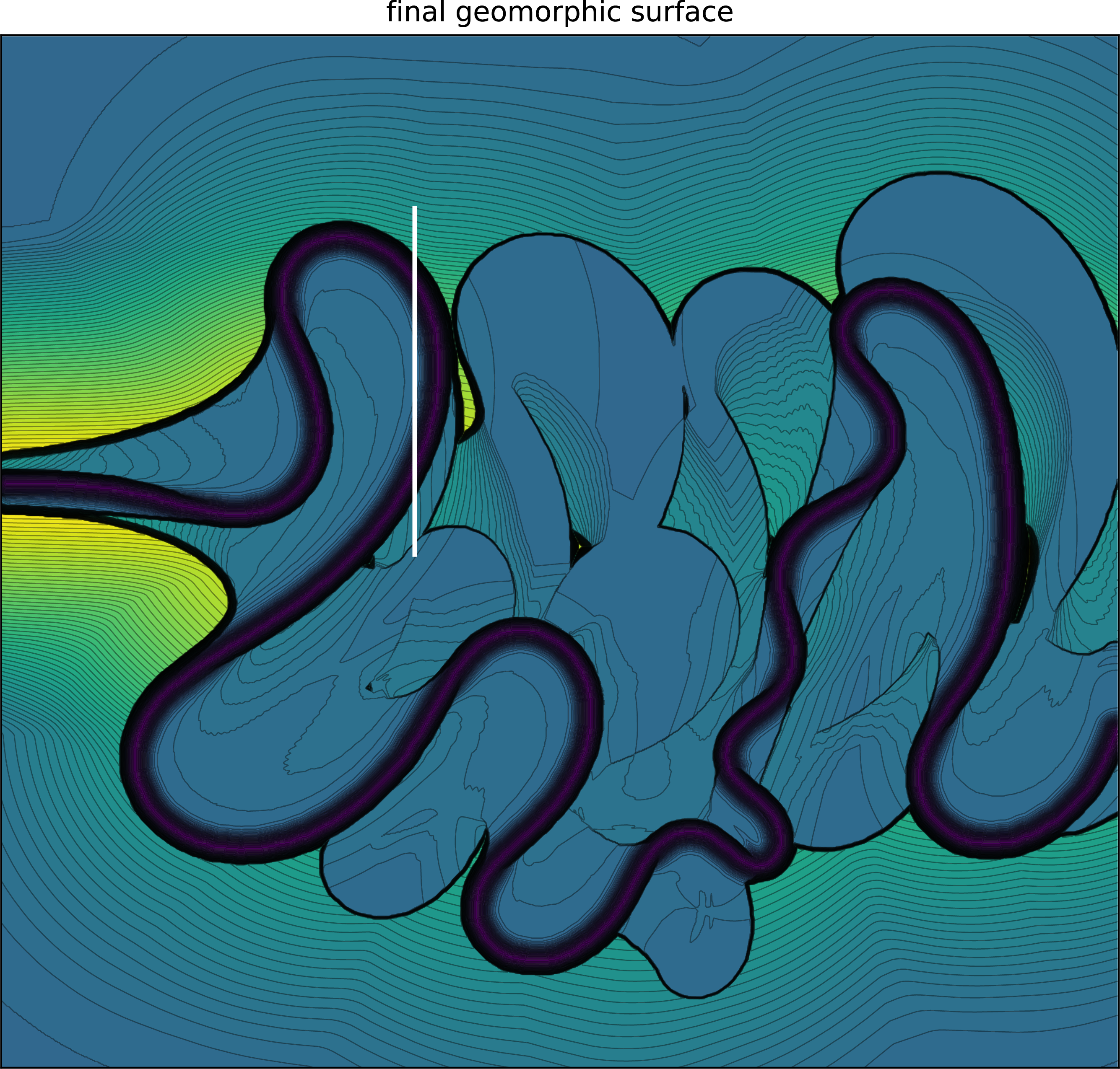 116 |
117 |
116 |
117 | 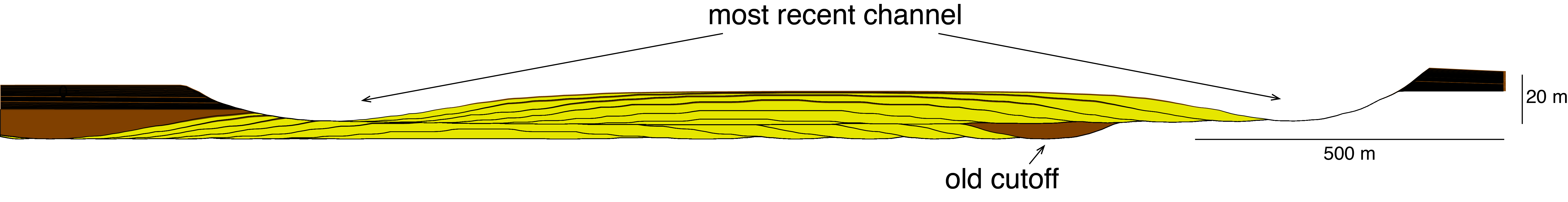 118 |
119 | ## Google Colab notebook
120 |
121 | If you don't want to deal with any local Python environments and installations, you should be able to run meanderpy in [this Google Colab notebook](https://colab.research.google.com/drive/1eZgGD_eXddaAeqxmI9guGIcTjjrLXmKO?usp=sharing).
122 |
123 | ## Related publications
124 |
125 | If you use meanderpy in your work, please consider citing one or more of these publications:
126 |
127 | Sylvester, Z., Durkin, P., and Covault, J.A., 2019, High curvatures drive river meandering: Geology, v. 47, p. 263–266, [doi:10.1130/G45608.1](https://doi.org/10.1130/G45608.1).
128 |
129 | Sylvester, Z., and Covault, J.A., 2016, Development of cutoff-related knickpoints during early evolution of submarine channels: Geology, v. 44, p. 835–838, [doi:10.1130/G38397.1](https://doi.org/10.1130/G38397.1).
130 |
131 | Covault, J.A., Sylvester, Z., Hubbard, S.M., and Jobe, Z.R., 2016, The Stratigraphic Record of Submarine-Channel Evolution: The Sedimentary Record, v. 14, no. 3, p. 4-11, [doi:10.2210/sedred.2016.3](https://www.sepm.org/files/143article.hqx9r9brxux8f2se.pdf).
132 |
133 | Sylvester, Z., Pirmez, C., and Cantelli, A., 2011, A model of submarine channel-levee evolution based on channel trajectories: Implications for stratigraphic architecture: Marine and Petroleum Geology, v. 28, p. 716–727, [doi:10.1016/j.marpetgeo.2010.05.012](https://doi.org/10.1016/j.marpetgeo.2010.05.012).
134 |
135 | ## Acknowledgements
136 |
137 | While the code in 'meanderpy' was written relatively recently, many of the ideas implemented in it come from numerous discussions with Carlos Pirmez, Alessandro Cantelli, Matt Wolinsky, Nick Howes, and Jake Covault. Funding for this work comes from the [Quantitative Clastics Laboratory industrial consortium](http://www.beg.utexas.edu/qcl) at the Bureau of Economic Geology, The University of Texas at Austin.
138 |
139 | ## License
140 |
141 | meanderpy is licensed under the [Apache License 2.0](https://github.com/zsylvester/meanderpy/blob/master/LICENSE.txt).
142 |
--------------------------------------------------------------------------------
/define_3D_domain.png:
--------------------------------------------------------------------------------
https://raw.githubusercontent.com/zsylvester/meanderpy/10938b0eafab77830304185d380dd1751c758d8b/define_3D_domain.png
--------------------------------------------------------------------------------
/fluvial_meanderpy_example_map.png:
--------------------------------------------------------------------------------
https://raw.githubusercontent.com/zsylvester/meanderpy/10938b0eafab77830304185d380dd1751c758d8b/fluvial_meanderpy_example_map.png
--------------------------------------------------------------------------------
/fluvial_meanderpy_example_section.png:
--------------------------------------------------------------------------------
https://raw.githubusercontent.com/zsylvester/meanderpy/10938b0eafab77830304185d380dd1751c758d8b/fluvial_meanderpy_example_section.png
--------------------------------------------------------------------------------
/meanderpy/.gitignore:
--------------------------------------------------------------------------------
1 | .DS_Store
2 |
--------------------------------------------------------------------------------
/meanderpy/__init__.py:
--------------------------------------------------------------------------------
1 | name = "meanderpy"
2 | from .meanderpy import *
--------------------------------------------------------------------------------
/meanderpy/meanderpy.ipynb:
--------------------------------------------------------------------------------
1 | {
2 | "cells": [
3 | {
4 | "cell_type": "code",
5 | "execution_count": 1,
6 | "metadata": {},
7 | "outputs": [],
8 | "source": [
9 | "import meanderpy as mp\n",
10 | "import matplotlib.pyplot as plt\n",
11 | "import numpy as np\n",
12 | "%matplotlib qt"
13 | ]
14 | },
15 | {
16 | "cell_type": "code",
17 | "execution_count": 6,
18 | "metadata": {},
19 | "outputs": [
20 | {
21 | "data": {
22 | "text/plain": [
23 | ""
24 | ]
25 | },
26 | "execution_count": 6,
27 | "metadata": {},
28 | "output_type": "execute_result"
29 | }
30 | ],
31 | "source": [
32 | "from importlib import reload\n",
33 | "reload(mp)"
34 | ]
35 | },
36 | {
37 | "cell_type": "markdown",
38 | "metadata": {},
39 | "source": [
40 | "## Input parameters"
41 | ]
42 | },
43 | {
44 | "cell_type": "code",
45 | "execution_count": 3,
46 | "metadata": {},
47 | "outputs": [],
48 | "source": [
49 | "nit = 2000 # number of iterations\n",
50 | "W = 200.0 # channel width (m)\n",
51 | "D = 6.0 # channel depth (m)\n",
52 | "depths = D * np.ones((nit,)) # channel depths for different iterations \n",
53 | "pad = 100 # padding (number of nodepoints along centerline)\n",
54 | "deltas = 50.0 # sampling distance along centerline \n",
55 | "Cfs = 0.011 * np.ones((nit,)) # dimensionless Chezy friction factor\n",
56 | "crdist = 2 * W # threshold distance at which cutoffs occur\n",
57 | "kl = 60.0/(365*24*60*60.0) # migration rate constant (m/s)\n",
58 | "kv = 1.0e-11 # vertical slope-dependent erosion rate constant (m/s)\n",
59 | "dt = 2*0.05*365*24*60*60.0 # time step (s)\n",
60 | "dens = 1000 # density of water (kg/m3)\n",
61 | "saved_ts = 20 # which time steps will be saved\n",
62 | "n_bends = 30 # approximate number of bends you want to model\n",
63 | "Sl = 0.002 # initial slope (matters more for submarine channels than rivers)\n",
64 | "t1 = 500 # time step when incision starts\n",
65 | "t2 = 700 # time step when lateral migration starts\n",
66 | "t3 = 1200 # time step when aggradation starts\n",
67 | "aggr_factor = 2e-9 # aggradation factor (m/s, about 0.18 m/year, it kicks in after t3)"
68 | ]
69 | },
70 | {
71 | "cell_type": "markdown",
72 | "metadata": {},
73 | "source": [
74 | "## Initialize model"
75 | ]
76 | },
77 | {
78 | "cell_type": "code",
79 | "execution_count": 7,
80 | "metadata": {},
81 | "outputs": [],
82 | "source": [
83 | "ch = mp.generate_initial_channel(W, depths[0], Sl, deltas, pad, n_bends) # initialize channel\n",
84 | "chb = mp.ChannelBelt(channels=[ch], cutoffs=[], cl_times=[0.0], cutoff_times=[]) # create channel belt object"
85 | ]
86 | },
87 | {
88 | "cell_type": "markdown",
89 | "metadata": {},
90 | "source": [
91 | "## Run simulation"
92 | ]
93 | },
94 | {
95 | "cell_type": "code",
96 | "execution_count": 8,
97 | "metadata": {},
98 | "outputs": [
99 | {
100 | "name": "stderr",
101 | "output_type": "stream",
102 | "text": [
103 | "100%|███████████████████████████████████████| 2000/2000 [00:21<00:00, 91.67it/s]\n"
104 | ]
105 | }
106 | ],
107 | "source": [
108 | "chb.migrate(nit,saved_ts,deltas,pad,crdist,depths,Cfs,kl,kv,dt,dens) #,t1,t2,t3,aggr_factor) # channel migration\n",
109 | "fig = chb.plot('strat', 20, 60, chb.cl_times[-1], len(chb.channels)) # plotting"
110 | ]
111 | },
112 | {
113 | "cell_type": "code",
114 | "execution_count": 9,
115 | "metadata": {},
116 | "outputs": [],
117 | "source": [
118 | "# check the z-profiles (to see whether there is the right amount of incision/aggradation):\n",
119 | "plt.figure()\n",
120 | "for channel in chb.channels:\n",
121 | " plt.plot(channel.x, channel.z, 'k', linewidth=0.5)"
122 | ]
123 | },
124 | {
125 | "cell_type": "markdown",
126 | "metadata": {},
127 | "source": [
128 | "Create a \"geomorphologic\" display that takes into account that older point bars and cutoffs are covered by vegetation:"
129 | ]
130 | },
131 | {
132 | "cell_type": "code",
133 | "execution_count": 10,
134 | "metadata": {},
135 | "outputs": [],
136 | "source": [
137 | "fig = chb.plot('morph', 20, 60, chb.cl_times[-1], len(chb.channels))"
138 | ]
139 | },
140 | {
141 | "cell_type": "markdown",
142 | "metadata": {},
143 | "source": [
144 | "Create a map that is colored by the age of the point bars:"
145 | ]
146 | },
147 | {
148 | "cell_type": "code",
149 | "execution_count": 14,
150 | "metadata": {},
151 | "outputs": [],
152 | "source": [
153 | "fig = chb.plot('age', 20, 60, chb.cl_times[-1], len(chb.channels))"
154 | ]
155 | },
156 | {
157 | "cell_type": "markdown",
158 | "metadata": {},
159 | "source": [
160 | "## Create movie"
161 | ]
162 | },
163 | {
164 | "cell_type": "code",
165 | "execution_count": 9,
166 | "metadata": {},
167 | "outputs": [],
168 | "source": [
169 | "dirname = '/Users/zoltan/Dropbox/Channels/temp/'\n",
170 | "chb.create_movie(xmin=10000, xmax=30000, plot_type='strat', filename='movie', dirname=dirname,\n",
171 | " pb_age = 1, ob_age = 20, end_time = chb.cl_times[-1], n_channels = len(chb.channels))"
172 | ]
173 | },
174 | {
175 | "cell_type": "markdown",
176 | "metadata": {},
177 | "source": [
178 | "## Build 3D fluvial model\n",
179 | "\n",
180 | "### Non-interactive definition of x- and y-extent\n",
181 | "\n",
182 | "If the parameters 'xmin', 'xmax', ymin', and 'ymax' are non-zero (as in the cell below), they will be used to define the extent of the area of interest used to build the 3D model. At least initially, it is a good idea to keep this segment relatively small (only a few bends long) to avoid building very large models."
183 | ]
184 | },
185 | {
186 | "cell_type": "code",
187 | "execution_count": 15,
188 | "metadata": {},
189 | "outputs": [
190 | {
191 | "name": "stderr",
192 | "output_type": "stream",
193 | "text": [
194 | "100%|█████████████████████████████████████████| 100/100 [00:39<00:00, 2.50it/s]"
195 | ]
196 | },
197 | {
198 | "name": "stdout",
199 | "output_type": "stream",
200 | "text": [
201 | "43.98457647341001\n"
202 | ]
203 | },
204 | {
205 | "name": "stderr",
206 | "output_type": "stream",
207 | "text": [
208 | "\n"
209 | ]
210 | }
211 | ],
212 | "source": [
213 | "h_mud = 2.0 * np.ones((len(chb.channels),)) # thickness of overbank deposit for each time step\n",
214 | "dx = 10.0 # gridcell size in meters\n",
215 | "diff_scale = 1.0 * W/dx\n",
216 | "v_coarse = 8.0 # deposition rate of coarse overbank sediment, in m/year (excluding times of no flooding)\n",
217 | "v_fine = 0.0 # deposition rate of fine overbank sediment, in m/year (excluding times of no flooding)\n",
218 | "\n",
219 | "chb_3d, xmin, xmax, ymin, ymax, dists, zmaps = mp.build_3d_model(chb, 'fluvial', \n",
220 | " h_mud=h_mud, h=12.0, w=W, dx=dx, delta_s=deltas, dt=dt, \n",
221 | " starttime=chb.cl_times[0], endtime=chb.cl_times[-1],\n",
222 | " diff_scale=diff_scale, v_fine=v_fine, v_coarse=v_coarse, \n",
223 | " xmin=15000, xmax=20000, ymin=-3500, ymax=3500)"
224 | ]
225 | },
226 | {
227 | "cell_type": "code",
228 | "execution_count": 17,
229 | "metadata": {},
230 | "outputs": [],
231 | "source": [
232 | "# create plots\n",
233 | "fig1,fig2,fig3 = chb_3d.plot_xsection(300, [[0.9,0.9,0],[0.5,0.25,0]], 4)"
234 | ]
235 | },
236 | {
237 | "cell_type": "markdown",
238 | "metadata": {},
239 | "source": [
240 | "## Build fluvial model with variable depths and well-defined scrolls"
241 | ]
242 | },
243 | {
244 | "cell_type": "code",
245 | "execution_count": 25,
246 | "metadata": {},
247 | "outputs": [
248 | {
249 | "name": "stderr",
250 | "output_type": "stream",
251 | "text": [
252 | "100%|███████████████████████████████████████| 2000/2000 [00:22<00:00, 90.27it/s]\n"
253 | ]
254 | }
255 | ],
256 | "source": [
257 | "nit = 2000 # number of iterations\n",
258 | "W = 200.0 # channel width (m)\n",
259 | "D = 6.0\n",
260 | "saved_ts = 20 # which time steps will be saved# channel depth (m)\n",
261 | "# create variable depth sequence:\n",
262 | "depths = D * np.ones((nit,)) + np.repeat(1.5*(np.random.random_sample(int(nit/saved_ts))-0.5), saved_ts)\n",
263 | "pad = 100 # padding (number of nodepoints along centerline)\n",
264 | "deltas = 50.0 # sampling distance along centerline \n",
265 | "Cfs = 0.011 * np.ones((nit,)) # dimensionless Chezy friction factor\n",
266 | "crdist = 2 * W # threshold distance at which cutoffs occur\n",
267 | "kl = 60.0/(365*24*60*60.0) # migration rate constant (m/s)\n",
268 | "kv = 1.0e-12 # vertical slope-dependent erosion rate constant (m/s)\n",
269 | "dt = 2*0.05*365*24*60*60.0 # time step (s)\n",
270 | "dens = 1000 # density of water (kg/m3)\n",
271 | "n_bends = 30 # approximate number of bends you want to model\n",
272 | "Sl = 0.00 # initial slope (matters more for submarine channels than rivers)\n",
273 | "\n",
274 | "ch = mp.generate_initial_channel(W, depths[0], Sl, deltas, pad, n_bends) # initialize channel\n",
275 | "chb = mp.ChannelBelt(channels=[ch], cutoffs=[], cl_times=[0.0], cutoff_times=[]) # create channel belt object\n",
276 | "\n",
277 | "chb.migrate(nit,saved_ts,deltas,pad,crdist,depths,Cfs,kl,kv,dt,dens) # channel migration\n",
278 | "fig = chb.plot('strat', 20, 60, chb.cl_times[-1], len(chb.channels)) # plotting"
279 | ]
280 | },
281 | {
282 | "cell_type": "code",
283 | "execution_count": 27,
284 | "metadata": {
285 | "tags": []
286 | },
287 | "outputs": [
288 | {
289 | "name": "stderr",
290 | "output_type": "stream",
291 | "text": [
292 | "100%|█████████████████████████████████████████| 100/100 [01:07<00:00, 1.48it/s]\n"
293 | ]
294 | }
295 | ],
296 | "source": [
297 | "# add a bit more incision:\n",
298 | "for i in range(len(chb.channels)):\n",
299 | " chb.channels[i].z = np.ones(np.shape(chb.channels[i].x))*(-0.1 * i)\n",
300 | "# create 'h_mud' sequence that mimicks the varibaility in depth through time:\n",
301 | "depths1 = depths[::saved_ts]\n",
302 | "depths1 = np.hstack((depths1[0], depths1))\n",
303 | "h_mud = depths1 - 5.0 # maximum thickness of overbank deposit for each time step\n",
304 | "dx = 10.0 # gridcell size in meters\n",
305 | "# reduce diffusion length scale:\n",
306 | "diff_scale = 1.0 * W/dx\n",
307 | "# increase deposition rate of coares sediment:\n",
308 | "v_coarse = 20.0 # deposition rate of coarse overbank sediment, in m/year (excluding times of no flooding)\n",
309 | "v_fine = 0.0 # deposition rate of fine overbank sediment, in m/year (excluding times of no flooding)"
310 | ]
311 | },
312 | {
313 | "cell_type": "markdown",
314 | "metadata": {},
315 | "source": [
316 | "## Interactive definition of x- and y-extent\n",
317 | "After you run the next cell, you need to select the upper left and lower right corners of the area of interest for which you want to build a 3D model. At least initially, it is a good idea to keep this segment relatively small (only a few bends long) to avoid building very large models. The area will only be highlighted (as a red rectangle) after the 3d model building has finished."
318 | ]
319 | },
320 | {
321 | "cell_type": "code",
322 | "execution_count": 23,
323 | "metadata": {},
324 | "outputs": [
325 | {
326 | "name": "stderr",
327 | "output_type": "stream",
328 | "text": [
329 | "100%|█████████████████████████████████████████| 100/100 [01:00<00:00, 1.65it/s]\n"
330 | ]
331 | }
332 | ],
333 | "source": [
334 | "chb_3d, xmin, xmax, ymin, ymax, dists, zmaps = mp.build_3d_model(chb, 'fluvial', \n",
335 | " h_mud=h_mud, h=12.0, w=W, \n",
336 | " bth=0.0, dcr=10.0, dx=dx, delta_s=deltas, dt=dt, starttime=chb.cl_times[0], endtime=chb.cl_times[-1],\n",
337 | " diff_scale=diff_scale, v_fine=v_fine, v_coarse=v_coarse)\n",
338 | "\n",
339 | "# create plots\n",
340 | "fig1,fig2,fig3 = chb_3d.plot_xsection(200, [[0.9,0.9,0],[0.5,0.25,0]], 4)"
341 | ]
342 | },
343 | {
344 | "cell_type": "markdown",
345 | "metadata": {},
346 | "source": [
347 | "## Build 3D submarine channel model"
348 | ]
349 | },
350 | {
351 | "cell_type": "code",
352 | "execution_count": 42,
353 | "metadata": {},
354 | "outputs": [],
355 | "source": [
356 | "reload(mp)\n",
357 | "nit = 2000 # number of iterations\n",
358 | "W = 200.0 # channel width (m)\n",
359 | "D = 6.0 # channel depth (m)\n",
360 | "depths = D * np.ones((nit,)) # channel depths for different iterations \n",
361 | "pad = 50 # padding (number of nodepoints along centerline)\n",
362 | "deltas = W/4 # sampling distance along centerline \n",
363 | "Cfs = 0.011 * np.ones((nit,)) # dimensionless Chezy friction factor\n",
364 | "crdist = 1.5 * W # threshold distance at which cutoffs occur\n",
365 | "kl = 60.0/(365*24*60*60.0) # migration rate constant (m/s)\n",
366 | "kv = 1.0e-12 # vertical slope-dependent erosion rate constant (m/s)\n",
367 | "dt = 2*0.05*365*24*60*60.0 # time step (s)\n",
368 | "dens = 1000 # density of water (kg/m3)\n",
369 | "saved_ts = 20 # which time steps will be saved\n",
370 | "n_bends = 30 # approximate number of bends you want to model\n",
371 | "Sl = 0.01 # initial slope (matters more for submarine channels than rivers)"
372 | ]
373 | },
374 | {
375 | "cell_type": "code",
376 | "execution_count": 43,
377 | "metadata": {},
378 | "outputs": [],
379 | "source": [
380 | "ch = mp.generate_initial_channel(W, depths[0], Sl, deltas, pad, n_bends) # initialize channel\n",
381 | "chb = mp.ChannelBelt(channels=[ch], cutoffs=[], cl_times=[0.0], cutoff_times=[]) # create channel belt object"
382 | ]
383 | },
384 | {
385 | "cell_type": "code",
386 | "execution_count": 44,
387 | "metadata": {},
388 | "outputs": [
389 | {
390 | "name": "stderr",
391 | "output_type": "stream",
392 | "text": [
393 | "100%|███████████████████████████████████████| 2000/2000 [00:23<00:00, 84.27it/s]\n"
394 | ]
395 | }
396 | ],
397 | "source": [
398 | "# chb.migrate(nit,saved_ts,deltas,pad,crdist,depths,Cfs,kl,kv,dt,dens,t1,t2,t3,aggr_factor) # channel migration\n",
399 | "chb.migrate(nit, saved_ts, deltas, pad, crdist, depths, Cfs, kl, kv, dt, dens)\n",
400 | "fig = chb.plot('strat',20,60,chb.cl_times[-1],len(chb.channels)) # plotting"
401 | ]
402 | },
403 | {
404 | "cell_type": "markdown",
405 | "metadata": {},
406 | "source": [
407 | "After you run the next cell, you need to select the upper left and lower right corners of the area of interest for which you want to build a 3D model. At least initially, it is a good idea to keep this segment relatively small (only a few bends long) to avoid building very large models. The area will only be highlighted (as a red rectangle) after the 3d model building has finished."
408 | ]
409 | },
410 | {
411 | "cell_type": "code",
412 | "execution_count": 45,
413 | "metadata": {},
414 | "outputs": [
415 | {
416 | "name": "stderr",
417 | "output_type": "stream",
418 | "text": [
419 | "100%|█████████████████████████████████████████| 100/100 [03:21<00:00, 2.01s/it]\n"
420 | ]
421 | }
422 | ],
423 | "source": [
424 | "h_mud = 4.0 * np.ones((len(chb.cl_times),)) # thickness of overbank deposit for each time step\n",
425 | "dx = 10.0 # gridcell size in meters\n",
426 | "diff_scale = 3 * W/dx\n",
427 | "v_coarse = 4.0 # deposition rate of coarse overbank sediment, in m/year (excluding times of no flow in channel)\n",
428 | "v_fine = 0.0 # deposition rate of fine overbank sediment, in m/year (excluding times of no flow in channel)\n",
429 | "\n",
430 | "chb_3d, xmin, xmax, ymin, ymax, dists, zmaps = mp.build_3d_model(chb, \n",
431 | " 'submarine', h_mud=h_mud, h=15.0, w=W, \n",
432 | " bth=4.0, dcr=6.0, dx=dx, delta_s=deltas, dt=dt, starttime=chb.cl_times[0], endtime=chb.cl_times[-1],\n",
433 | " diff_scale=diff_scale, v_fine=v_fine, v_coarse=v_coarse)"
434 | ]
435 | },
436 | {
437 | "cell_type": "code",
438 | "execution_count": 47,
439 | "metadata": {},
440 | "outputs": [],
441 | "source": [
442 | "fig1,fig2,fig3 = chb_3d.plot_xsection(1000, [[0.9,0.9,0], [0.5,0.25,0]], 10)"
443 | ]
444 | }
445 | ],
446 | "metadata": {
447 | "kernelspec": {
448 | "display_name": "Python 3 (ipykernel)",
449 | "language": "python",
450 | "name": "python3"
451 | },
452 | "language_info": {
453 | "codemirror_mode": {
454 | "name": "ipython",
455 | "version": 3
456 | },
457 | "file_extension": ".py",
458 | "mimetype": "text/x-python",
459 | "name": "python",
460 | "nbconvert_exporter": "python",
461 | "pygments_lexer": "ipython3",
462 | "version": "3.11.4"
463 | }
464 | },
465 | "nbformat": 4,
466 | "nbformat_minor": 4
467 | }
468 |
--------------------------------------------------------------------------------
/meanderpy/meanderpy.py:
--------------------------------------------------------------------------------
1 | import numpy as np
2 | import matplotlib.pyplot as plt
3 | import scipy.interpolate
4 | from scipy.spatial import distance
5 | from scipy import ndimage
6 | from PIL import Image, ImageDraw
7 | from skimage import measure
8 | from skimage import morphology
9 | # from skimage import filters
10 | from scipy.ndimage import gaussian_filter
11 | from matplotlib.colors import LinearSegmentedColormap
12 | import time, sys
13 | import numba
14 | import matplotlib.colors as mcolors
15 | from matplotlib import cm
16 | from tqdm import trange
17 | import h5py
18 | from scipy.signal import savgol_filter
19 |
20 |
21 | class Channel:
22 | """class for Channel objects"""
23 |
24 | def __init__(self,x,y,z,W,D):
25 | """
26 | Initialize Channel object.
27 |
28 | Parameters
29 | ----------
30 | x : array_like
31 | x-coordinate of centerline.
32 | y : array_like
33 | y-coordinate of centerline.
34 | z : array_like
35 | z-coordinate of centerline.
36 | W : float
37 | Channel width.
38 | D : float
39 | Channel depth.
40 | """
41 |
42 | self.x = x
43 | self.y = y
44 | self.z = z
45 | self.W = W
46 | self.D = D
47 |
48 | class Cutoff:
49 | """class for Cutoff objects"""
50 |
51 | def __init__(self,x,y,z,W,D):
52 | """
53 | Initialize Cutoff object.
54 |
55 | Parameters
56 | ----------
57 | x : array_like
58 | x-coordinate of centerline.
59 | y : array_like
60 | y-coordinate of centerline.
61 | z : array_like
62 | z-coordinate of centerline.
63 | W : float
64 | Channel width.
65 | D : float
66 | Channel depth.
67 | """
68 |
69 | self.x = x
70 | self.y = y
71 | self.z = z
72 | self.W = W
73 | self.D = D
74 |
75 | class ChannelBelt3D:
76 | """class for 3D models of channel belts"""
77 |
78 | def __init__(self, model_type, topo, strat, facies, facies_code, dx, channels):
79 | """
80 | Initialize ChannelBelt3D object.
81 |
82 | Parameters
83 | ----------
84 | model_type : str
85 | Type of model to be built; can be either 'fluvial' or 'submarine'.
86 | topo : numpy.ndarray
87 | Set of topographic surfaces (3D numpy array).
88 | strat : numpy.ndarray
89 | Set of stratigraphic surfaces (3D numpy array).
90 | facies : numpy.ndarray
91 | Facies volume (3D numpy array).
92 | facies_code : dict
93 | Dictionary of facies codes, e.g. {0:'oxbow', 1:'point bar', 2:'levee'}.
94 | dx : float
95 | Gridcell size (m).
96 | channels : list
97 | List of channel objects that form 3D model.
98 | """
99 |
100 | self.model_type = model_type
101 | self.topo = topo
102 | self.strat = strat
103 | self.facies = facies
104 | self.facies_code = facies_code
105 | self.dx = dx
106 | self.channels = channels
107 |
108 | def plot_xsection(self, xsec, colors, ve):
109 | """
110 | Method for plotting a cross section through a 3D model; also plots map of
111 | basal erosional surface and map of final geomorphic surface.
112 |
113 | Parameters
114 | ----------
115 | xsec : int
116 | Location of cross section along the x-axis (in pixel/voxel coordinates).
117 | colors : list of tuple
118 | List of RGB values that define the colors for different facies.
119 | ve : float
120 | Vertical exaggeration.
121 |
122 | Returns
123 | -------
124 | fig1 : matplotlib.figure.Figure
125 | Figure handle for the cross section plot.
126 | fig2 : matplotlib.figure.Figure
127 | Figure handle for the final geomorphic surface plot.
128 | fig3 : matplotlib.figure.Figure
129 | Figure handle for the basal erosional surface plot.
130 | """
131 |
132 | strat = self.strat
133 | dx = self.dx
134 | fig1 = plt.figure(figsize=(20,5))
135 | ax1 = fig1.add_subplot(111)
136 | r,c,ts = np.shape(strat)
137 | Xv = dx * np.arange(0,r)
138 | for i in range(0,ts-1,2):
139 | X1 = np.concatenate((Xv, Xv[::-1]))
140 | Y1 = np.concatenate((strat[:,xsec,i], strat[::-1,xsec,i+1]))
141 | Y2 = np.concatenate((strat[:,xsec,i+1], strat[::-1,xsec,i+2]))
142 | # Y3 = np.concatenate((strat[:,xsec,i+2], strat[::-1,xsec,i+3]))
143 | if self.model_type == 'submarine':
144 | ax1.fill(X1, Y1, facecolor=colors[0], linewidth=0.5, edgecolor=[0,0,0]) # channel sand
145 | ax1.fill(X1, Y2, facecolor=colors[1], linewidth=0.5, edgecolor=[0,0,0]) # levee mud
146 | if self.model_type == 'fluvial':
147 | ax1.fill(X1, Y1, facecolor=colors[0], linewidth=0.5, edgecolor=[0,0,0]) # channel sand
148 | ax1.fill(X1, Y2, facecolor=colors[1], linewidth=0.5, edgecolor=[0,0,0]) # levee mud
149 | # ax1.fill(X1, Y3, facecolor=colors[2], linewidth=0.5) # channel sand
150 | ax1.set_xlim(0,dx*(r-1))
151 | ax1.set_aspect(ve, adjustable='datalim')
152 | fig2 = plt.figure()
153 | ax2 = fig2.add_subplot(111)
154 | ax2.contourf(strat[:,:,ts-1],100,cmap='viridis')
155 | ax2.contour(strat[:,:,ts-1],100,colors='k',linestyles='solid',linewidths=0.1,alpha=0.4)
156 | ax2.plot([xsec, xsec],[0,r],'k',linewidth=2)
157 | ax2.axis([0,c,0,r])
158 | ax2.set_aspect('equal', adjustable='box')
159 | ax2.set_title('final geomorphic surface')
160 | ax2.tick_params(bottom=False,top=False,left=False,right=False,labelbottom=False,labelleft=False)
161 | fig3 = plt.figure()
162 | ax3 = fig3.add_subplot(111)
163 | ax3.contourf(strat[:,:,0],100,cmap='viridis')
164 | ax3.contour(strat[:,:,0],100,colors='k',linestyles='solid',linewidths=0.1,alpha=0.4)
165 | ax3.plot([xsec, xsec],[0,r],'k',linewidth=2)
166 | ax3.axis([0,c,0,r])
167 | ax3.set_aspect('equal', adjustable='box')
168 | ax3.set_title('basal erosional surface')
169 | ax3.tick_params(bottom=False,top=False,left=False,right=False,labelbottom=False,labelleft=False)
170 | return fig1, fig2, fig3
171 |
172 | class ChannelBelt:
173 | """class for ChannelBelt objects"""
174 |
175 | def __init__(self, channels, cutoffs, cl_times, cutoff_times):
176 | """
177 | Initialize ChannelBelt object.
178 |
179 | Parameters
180 | ----------
181 | channels : list of Channel
182 | List of Channel objects.
183 | cutoffs : list of Cutoff
184 | List of Cutoff objects.
185 | cl_times : list of float
186 | List of ages of Channel objects (in years).
187 | cutoff_times : list of float
188 | List of ages of Cutoff objects.
189 | """
190 |
191 | self.channels = channels
192 | self.cutoffs = cutoffs
193 | self.cl_times = cl_times
194 | self.cutoff_times = cutoff_times
195 |
196 | def migrate(self, nit, saved_ts, deltas, pad, crdist, depths, Cfs, kl, kv, dt, dens, autoaggradation=True, Scr=0.001, t1=None, t2=None, t3=None, aggr_factor=None):
197 | """
198 | Compute migration rates along channel centerlines and move the centerlines accordingly.
199 |
200 | Parameters
201 | ----------
202 | nit : int
203 | Number of iterations.
204 | saved_ts : int
205 | Which time steps will be saved; e.g., if saved_ts = 10, every tenth time step will be saved.
206 | deltas : float
207 | Distance between nodes on centerline.
208 | pad : int
209 | Padding (number of nodepoints along centerline).
210 | crdist : float
211 | Threshold distance at which cutoffs occur.
212 | depths : array_like
213 | Array of channel depths (can vary across iterations).
214 | Cfs : array_like
215 | Array of dimensionless Chezy friction factors (can vary across iterations).
216 | kl : float
217 | Migration rate constant (m/s).
218 | kv : float
219 | Vertical slope-dependent erosion rate constant (m/s).
220 | dt : float
221 | Time step (s).
222 | dens : float
223 | Density of fluid (kg/m^3).
224 | autoaggradation : bool, optional
225 | If True, autoaggradation is applied. Default is True.
226 | Scr : float, optional
227 | Critical slope for autoaggradation. Default is 0.001.
228 | t1 : int, optional
229 | Time step when incision starts. Default is None.
230 | t2 : int, optional
231 | Time step when lateral migration starts. Default is None.
232 | t3 : int, optional
233 | Time step when aggradation starts. Default is None.
234 | aggr_factor : float, optional
235 | Aggradation factor. Default is None.
236 | """
237 |
238 | channel = self.channels[-1] # first channel is the same as last channel of input
239 | x = channel.x; y = channel.y; z = channel.z
240 | W = channel.W
241 | D = channel.D
242 | k = 1.0 # constant in HK equation
243 | xc = [] # initialize cutoff coordinates
244 | # determine age of last channel:
245 | if len(self.cl_times)>0:
246 | last_cl_time = self.cl_times[-1]
247 | else:
248 | last_cl_time = 0
249 | dx, dy, dz, ds, s = compute_derivatives(x,y,z)
250 | slope = np.gradient(z)/ds
251 | # padding at the beginning can be shorter than padding at the downstream end:
252 | pad1 = int(pad/10.0)
253 | if pad1<5:
254 | pad1 = 5
255 | for itn in trange(nit): # main loop
256 | D = depths[itn]
257 | Cf = Cfs[itn]
258 | x, y = migrate_one_step(x,y,z,W,kl,dt,k,Cf,D,pad,pad1)
259 | # x, y = migrate_one_step_w_bias(x,y,z,W,kl,dt,k,Cf,D,pad,pad1)
260 | x,y,z,xc,yc,zc = cut_off_cutoffs(x,y,z,s,crdist,deltas) # find and execute cutoffs
261 | x,y,z,dx,dy,dz,ds,s = resample_centerline(x,y,z,deltas) # resample centerline
262 | z = savgol_filter(z, 21, 2) # filter z-values - needed for autoaggradation
263 | slope = np.gradient(z)/ds # positive number
264 | if autoaggradation:
265 | if np.max(slope) > 0.001:
266 | R = 1.65; C = 0.1 # parameters for autoaggradation
267 | z = z + kv*dens*9.81*R*C*D*(Scr-slope)*dt # autoaggradation
268 | else:
269 | # for itn<=t1, z is unchanged; for itn>t1:
270 | if (itn>t1) & (itn<=t2): # incision
271 | if np.min(np.abs(slope))!=0: # if slope is not zero
272 | z = z + kv*dens*9.81*D*slope*dt
273 | else:
274 | z = z - kv*dens*9.81*D*dt*0.05 # if slope is zero
275 | if (itn>t2) & (itn<=t3): # lateral migration
276 | if np.min(np.abs(slope))!=0: # if slope is not zero
277 | # use the median slope to counterbalance incision:
278 | z = z + kv*dens*9.81*D*slope*dt - kv*dens*9.81*D*np.median(slope)*dt
279 | else:
280 | z = z # no change in z
281 | if (itn>t3): # aggradation
282 | if np.min(np.abs(slope))!=0: # if slope is not zero
283 | # 'aggr_factor' should be larger than 1 so that this leads to overall aggradation:
284 | z = z + kv*dens*9.81*D*slope*dt - aggr_factor*kv*dens*9.81*D*np.mean(slope)*dt
285 | else:
286 | z = z + aggr_factor*dt
287 | if len(xc)>0: # save cutoff data
288 | self.cutoff_times.append(last_cl_time+(itn+1)*dt/(365*24*60*60.0))
289 | cutoff = Cutoff(xc,yc,zc,W,D) # create cutoff object
290 | self.cutoffs.append(cutoff)
291 | # saving centerlines (with the exception of first channel):
292 | if (np.mod(itn, saved_ts) == 0) and (itn > 0):
293 | self.cl_times.append(last_cl_time+(itn+1)*dt/(365*24*60*60.0))
294 | channel = Channel(x,y,z,W,D) # create channel object
295 | self.channels.append(channel)
296 |
297 | def plot(self, plot_type, pb_age, ob_age, end_time, n_channels):
298 | """
299 | Method for plotting ChannelBelt object.
300 |
301 | Parameters
302 | ----------
303 | plot_type : str
304 | Can be either 'strat' (for stratigraphic plot), 'morph' (for morphologic plot), or 'age' (for age plot).
305 | pb_age : int
306 | Age of point bars (in years) at which they get covered by vegetation.
307 | ob_age : int
308 | Age of oxbow lakes (in years) at which they get covered by vegetation.
309 | end_time : int
310 | Age of last channel to be plotted (in years).
311 | n_channels : int
312 | Total number of channels (used in 'age' plots; can be larger than number of channels being plotted).
313 |
314 | Returns
315 | -------
316 | fig : matplotlib.figure.Figure
317 | Handle to the figure.
318 | """
319 |
320 | cot = np.array(self.cutoff_times)
321 | sclt = np.array(self.cl_times)
322 | if end_time>0:
323 | cot = cot[cot<=end_time]
324 | sclt = sclt[sclt<=end_time]
325 | times = np.sort(np.hstack((cot,sclt)))
326 | times = np.unique(times)
327 | order = 0 # variable for ordering objects in plot
328 | # set up min and max x and y coordinates of the plot:
329 | xmin = np.min(self.channels[0].x)
330 | xmax = np.max(self.channels[0].x)
331 | ymax = 0
332 | for i in range(len(self.channels)):
333 | ymax = max(ymax, np.max(np.abs(self.channels[i].y)))
334 | ymax = ymax+2*self.channels[0].W # add a bit of space on top and bottom
335 | ymin = -1*ymax
336 | # size figure so that its size matches the size of the model:
337 | fig = plt.figure(figsize=(20,(ymax-ymin)*20/(xmax-xmin)))
338 | if plot_type == 'morph':
339 | pb_crit = len(times[timestimes[-1]-pb_age:
358 | plt.fill(xm,ym,facecolor=pb_cmap(i/float(len(times)-1)),edgecolor='k',linewidth=0.2)
359 | else:
360 | plt.fill(xm,ym,facecolor=pb_cmap(i/float(len(times)-1)))
361 | if plot_type == 'strat':
362 | order += 1
363 | plt.fill(xm, ym, 'xkcd:light tan', edgecolor='k', linewidth=0.25, zorder=order)
364 | # plt.fill(xm, ym, 'xkcd:light tan', edgecolor='none', linewidth=0.25, zorder=order)
365 | if plot_type == 'age':
366 | order += 1
367 | plt.fill(xm,ym,facecolor=age_cmap(i/float(n_channels-1)),edgecolor='k',linewidth=0.1,zorder=order)
368 | if times[i] in cot:
369 | ind = np.where(cot==times[i])[0][0]
370 | for j in range(0,len(self.cutoffs[ind].x)):
371 | x1 = self.cutoffs[ind].x[j]
372 | y1 = self.cutoffs[ind].y[j]
373 | xm, ym = get_channel_banks(x1,y1,self.cutoffs[ind].W)
374 | if plot_type == 'morph':
375 | plt.fill(xm,ym,color=ob_cmap(i/float(len(times)-1)))
376 | if plot_type == 'strat':
377 | order = order+1
378 | plt.fill(xm, ym, 'xkcd:ocean blue', edgecolor='k', linewidth=0.25, zorder=order)
379 | # plt.fill(xm, ym, 'xkcd:ocean blue', edgecolor='none', linewidth=0.25, zorder=order)
380 | if plot_type == 'age':
381 | order += 1
382 | plt.fill(xm, ym, 'xkcd:sea blue', edgecolor='k', linewidth=0.1, zorder=order)
383 |
384 | x1 = self.channels[len(sclt)-1].x
385 | y1 = self.channels[len(sclt)-1].y
386 | xm, ym = get_channel_banks(x1,y1,self.channels[len(sclt)-1].W)
387 | order = order+1
388 | if plot_type == 'age':
389 | plt.fill(xm, ym, color='xkcd:sea blue', zorder=order, edgecolor='k', linewidth=0.1)
390 | else:
391 | plt.fill(xm, ym, color=(16/255.0,73/255.0,90/255.0), edgecolor='none', zorder=order) #,edgecolor='k')
392 | plt.axis('equal')
393 | # plt.xlim(xmin,xmax)
394 | # plt.ylim(ymin,ymax)
395 | plt.xticks([])
396 | plt.yticks([])
397 | plt.tight_layout()
398 | return fig
399 |
400 | def create_movie(self, xmin, xmax, plot_type, filename, dirname, pb_age, ob_age, end_time, n_channels):
401 | """
402 | Method for creating movie frames (PNG files) that capture the plan-view evolution of a channel belt through time.
403 | The movie has to be assembled from the PNG files after this method is applied.
404 |
405 | Parameters
406 | ----------
407 | xmin : float
408 | Value of x coordinate on the left side of the frame.
409 | xmax : float
410 | Value of x coordinate on the right side of the frame.
411 | plot_type : str
412 | Plot type; can be either 'strat' (for stratigraphic plot) or 'morph' (for morphologic plot).
413 | filename : str
414 | First few characters of the output filenames.
415 | dirname : str
416 | Name of the directory where output files should be written.
417 | pb_age : int
418 | Age of point bars (in years) at which they get covered by vegetation (if the 'morph' option is used for 'plot_type').
419 | ob_age : int
420 | Age of oxbow lakes (in years) at which they get covered by vegetation (if the 'morph' option is used for 'plot_type').
421 | end_time : float or list of float
422 | Time at which the simulation should be stopped.
423 | n_channels : int
424 | Total number of channels + cutoffs for which the simulation is run (usually it is len(chb.cutoffs) + len(chb.channels)). Used when plot_type = 'age'.
425 |
426 | """
427 |
428 | sclt = np.array(self.cl_times)
429 | if type(end_time) != list:
430 | sclt = sclt[sclt<=end_time]
431 | channels = self.channels[:len(sclt)]
432 | ymax = 0
433 | for i in range(len(channels)):
434 | ymax = max(ymax, np.max(np.abs(channels[i].y)))
435 | ymax = ymax+2*channels[0].W # add a bit of space on top and bottom
436 | ymin = -1*ymax
437 | for i in range(0,len(sclt)):
438 | fig = self.plot(plot_type, pb_age, ob_age, sclt[i], n_channels)
439 | scale = 1
440 | fig_height = scale*fig.get_figheight()
441 | fig_width = (xmax-xmin)*fig_height/(ymax-ymin)
442 | fig.set_figwidth(fig_width)
443 | fig.set_figheight(fig_height)
444 | fig.gca().set_xlim(xmin,xmax)
445 | fig.gca().set_xticks([])
446 | fig.gca().set_yticks([])
447 | plt.plot([xmin+200, xmin+200+5000],[ymin+200, ymin+200], 'k', linewidth=2)
448 | plt.text(xmin+200+2000, ymin+200+100, '5 km', fontsize=14)
449 | fname = dirname+filename+'%03d.png'%(i)
450 | fig.savefig(fname, bbox_inches='tight')
451 | plt.close()
452 |
453 | def build_3d_model(chb, model_type, h_mud, h, w, dx, delta_s, dt, starttime, endtime, diff_scale, v_fine, v_coarse, xmin=None, xmax=None, ymin=None, ymax=None, bth=None, dcr=None):
454 | """
455 | Build 3D model from set of centerlines (that are part of a ChannelBelt object).
456 |
457 | Parameters
458 | ----------
459 | model_type : str
460 | Model type ('fluvial' or 'submarine').
461 | h_mud : float
462 | Maximum thickness of overbank deposit.
463 | h : float
464 | Channel depth.
465 | w : float
466 | Channel width.
467 | dx : float
468 | Cell size in x and y directions.
469 | delta_s : float
470 | Sampling distance along centerlines.
471 | starttime : float
472 | Age of centerline that will be used as the first centerline in the model.
473 | endtime : float
474 | Age of centerline that will be used as the last centerline in the model.
475 | xmin : float, optional
476 | Minimum x coordinate that defines the model domain; if xmin is set to zero,
477 | a plot of the centerlines is generated and the model domain has to be defined by clicking its upper left and lower right corners.
478 | xmax : float, optional
479 | Maximum x coordinate that defines the model domain.
480 | ymin : float, optional
481 | Minimum y coordinate that defines the model domain.
482 | ymax : float, optional
483 | Maximum y coordinate that defines the model domain.
484 | diff_scale : float
485 | Diffusion length scale (for overbank deposition).
486 | v_fine : float
487 | Deposition rate of fine sediment, in m/year (for overbank deposition).
488 | v_coarse : float
489 | Deposition rate of coarse sediment, in m/year (for overbank deposition).
490 | bth : float, optional
491 | Thickness of channel sand (only used in submarine models).
492 | dcr : float, optional
493 | Critical channel depth where sand thickness goes to zero (only used in submarine models).
494 |
495 | Returns
496 | -------
497 | chb_3d : ChannelBelt3D
498 | A ChannelBelt3D object.
499 | xmin : float
500 | Minimum x coordinate that defines the model domain.
501 | xmax : float
502 | Maximum x coordinate that defines the model domain.
503 | ymin : float
504 | Minimum y coordinate that defines the model domain.
505 | ymax : float
506 | Maximum y coordinate that defines the model domain.
507 | """
508 |
509 | sclt = np.array(chb.cl_times)
510 | ind1 = np.where(sclt >= starttime)[0][0]
511 | ind2 = np.where(sclt <= endtime)[0][-1]
512 | sclt = sclt[ind1:ind2+1]
513 | channels = chb.channels[ind1:ind2+1]
514 | cot = np.array(chb.cutoff_times)
515 | if (len(cot)>0) and (len(np.where(cot >= starttime)[0])>0) and (len(np.where(cot <= endtime)[0])>0):
516 | cfind1 = np.where(cot >= starttime)[0][0]
517 | cfind2 = np.where(cot <= endtime)[0][-1]
518 | cot = cot[cfind1:cfind2+1]
519 | else:
520 | cot = []
521 | n_steps = len(sclt) # number of events
522 | if xmin is None: # plot centerlines and define model domain
523 | plt.figure(figsize=(15,10))
524 | for i in range(len(channels)): # plot centerlines
525 | plt.plot(chb.channels[i].x, chb.channels[i].y, 'k')
526 | if i == 0:
527 | maxX = np.max(channels[i].x)
528 | minX = np.min(channels[i].x)
529 | maxY = np.max(channels[i].y)
530 | minY = np.min(channels[i].y)
531 | else:
532 | maxX = max(maxX, np.max(channels[i].x))
533 | minX = min(minX, np.min(channels[i].x))
534 | maxY = max(maxY, np.max(channels[i].y))
535 | minY = min(minY, np.min(channels[i].y))
536 | plt.axis([minX, maxX, minY-10*w, maxY+10*w])
537 | plt.gca().set_aspect('equal', adjustable='box')
538 | plt.tight_layout()
539 | pts = np.zeros((2,2))
540 | for i in range(0,2):
541 | pt = np.asarray(plt.ginput(1))
542 | pts[i,:] = pt
543 | plt.scatter(pt[0][0], pt[0][1])
544 | plt.plot([pts[0,0], pts[1,0], pts[1,0], pts[0,0], pts[0,0]], [pts[0,1], pts[0,1], pts[1,1], pts[1,1], pts[0,1]], 'r')
545 | xmin = min(pts[0,0], pts[1,0])
546 | xmax = max(pts[0,0], pts[1,0])
547 | ymin = min(pts[0,1], pts[1,1])
548 | ymax = max(pts[0,1], pts[1,1])
549 | iwidth = int((xmax-xmin)/dx)
550 | iheight = int((ymax-ymin)/dx)
551 | topo = np.zeros((iheight, iwidth, 3*n_steps)) # array for storing topographic surfaces
552 | dists = np.zeros((iheight, iwidth, n_steps))
553 | zmaps = np.zeros((iheight, iwidth, n_steps))
554 | facies = np.zeros((3*n_steps, 1))
555 | # create initial topography:
556 | x1 = np.linspace(0, iwidth-1, iwidth)
557 | y1 = np.linspace(0, iheight-1, iheight)
558 | xv, yv = np.meshgrid(x1,y1)
559 | z1 = channels[0].z
560 | z1 = z1[(channels[0].x > xmin) & (channels[0].x < xmax)]
561 | topoinit = z1[0] - ((z1[0] - z1[-1]) / (xmax - xmin)) * xv * dx # initial (sloped) topography
562 | topo[:,:,0] = topoinit.copy()
563 | surf = topoinit.copy()
564 | facies[0] = np.NaN
565 | # generate surfaces:
566 | channels3D = []
567 | for i in trange(n_steps):
568 | x = channels[i].x
569 | y = channels[i].y
570 | z = channels[i].z
571 | cutoff_ind = []
572 | # check if there were cutoffs during the last time step and collect indices in an array:
573 | for j in range(len(cot)):
574 | if (cot[j] >= sclt[i-1]) & (cot[j] < sclt[i]):
575 | cutoff_ind.append(j)
576 | # create distance map:
577 | cl_dist, x_pix, y_pix, z_pix, s_pix, z_map, x1, y1, z1 = dist_map(x, y, z, xmin, xmax, ymin, ymax, dx, delta_s)
578 | # erosion:
579 | surf = np.minimum(surf, erosion_surface(h,w/dx,cl_dist,z_map))
580 | topo[:,:,3*i] = surf # erosional surface
581 | dists[:,:,i] = cl_dist # distance map
582 | zmaps[:,:,i] = z_map # map of closest channel elevation
583 | facies[3*i] = np.NaN # array for facies code
584 |
585 | if model_type == 'fluvial':
586 | z_map = gaussian_filter(z_map, sigma=50) # smooth z_map to avoid artefacts in levees
587 | pb = point_bar_surface(cl_dist, z_map, h, w/dx)
588 | th = np.maximum(surf,pb)-surf
589 | th[cl_dist > 1.0 * w/dx] = 0 # eliminate sand outside of channel
590 | th[th<0] = 0 # eliminate negative thickness values
591 | surf = surf+th # update topographic surface with sand thickness
592 | topo[:,:,3*i+1] = surf # top of sand
593 | facies[3*i+1] = 1 # facies code for point bar sand
594 | E_max = z_map + h_mud[i]
595 | if i == n_steps-1:
596 | surf_diff = E_max-surf
597 | surf_diff[surf_diff < 0] = 0
598 | plt.figure()
599 | plt.imshow(surf_diff)
600 | levee = fluvial_levee(cl_dist, surf, E_max, w/dx, diff_scale, v_fine, v_coarse, dt)
601 | if i == n_steps-1:
602 | plt.figure()
603 | plt.imshow(levee)
604 | surf = surf + levee # mud/levee deposition
605 | topo[:,:,3*i+2] = surf # top of levee
606 | facies[3*i+2] = 2 # facies code for overbank
607 | channels3D.append(Channel(x1-xmin, y1-ymin, z1, w, h))
608 |
609 | if model_type == 'submarine':
610 | z_map = gaussian_filter(z_map, sigma=50) # smooth z_map to avoid artefacts in levees
611 | th, relief = sand_surface(surf, bth, dcr, z_map, h) # sandy channel deposit
612 | th[th < 0] = 0 # eliminate negative thickness values
613 | ws = w * (dcr/h)**0.5 # channel width at the top of the channel deposit
614 | th[cl_dist > 1.0 * ws/dx] = 0 # eliminate sand outside of channel
615 | surf = surf+th # update topographic surface with sand thickness
616 | topo[:,:,3*i+1] = surf # top of sand
617 | facies[3*i+1] = 1 # facies code for channel sand
618 | # need to blur z-map so that levees don't have artefacts:
619 | # blurred = filters.gaussian(z_map, sigma=(50, 50), truncate=3.5, multichannel=False)
620 | E_max = z_map + h_mud[i]
621 | levee = submarine_levee(h_mud[i], cl_dist, surf, E_max, w/dx, diff_scale, v_fine, v_coarse, dt)
622 | surf = surf + levee # mud/levee deposition
623 | topo[:,:,3*i+2] = surf # top of levee
624 | facies[3*i+2] = 2 # facies code for overbank
625 | channels3D.append(Channel(x1-xmin, y1-ymin, z1, w, h))
626 |
627 | topo = np.concatenate((np.reshape(topoinit,(iheight,iwidth,1)),topo),axis=2) # add initial topography to array
628 | strat = topostrat(topo) # create stratigraphic surfaces
629 | strat = np.delete(strat, np.arange(3*n_steps+1)[1::3], 2) # get rid of unnecessary stratigraphic surfaces (duplicates)
630 | facies = np.delete(facies, np.arange(3*n_steps)[::3]) # get rid of unnecessary facies layers (NaNs)
631 | if model_type == 'fluvial':
632 | facies_code = {1:'point bar', 2:'levee'}
633 | if model_type == 'submarine':
634 | facies_code = {1:'channel sand', 2:'levee'}
635 | chb_3d = ChannelBelt3D(model_type, topo, strat, facies, facies_code, dx, channels3D)
636 | return chb_3d, xmin, xmax, ymin, ymax, dists, zmaps
637 |
638 | def resample_centerline(x,y,z,deltas):
639 | """
640 | Resample centerline so that 'deltas' is roughly constant, using parametric
641 | spline representation of curve; note that there is *no* smoothing.
642 |
643 | Parameters
644 | ----------
645 | x : array_like
646 | x-coordinates of centerline.
647 | y : array_like
648 | y-coordinates of centerline.
649 | z : array_like
650 | z-coordinates of centerline.
651 | deltas : float
652 | Distance between points on centerline.
653 |
654 | Returns
655 | -------
656 | x : ndarray
657 | x-coordinates of resampled centerline.
658 | y : ndarray
659 | y-coordinates of resampled centerline.
660 | z : ndarray
661 | z-coordinates of resampled centerline.
662 | dx : ndarray
663 | dx of resampled centerline.
664 | dy : ndarray
665 | dy of resampled centerline.
666 | dz : ndarray
667 | dz of resampled centerline.
668 | ds : ndarray
669 | ds of resampled centerline.
670 | s : ndarray
671 | s-coordinates of resampled centerline.
672 | """
673 |
674 | dx, dy, dz, ds, s = compute_derivatives(x,y,z) # compute derivatives
675 | tck, u = scipy.interpolate.splprep([x,y,z],s=0)
676 | unew = np.linspace(0,1,1+int(round(s[-1]/deltas))) # vector for resampling
677 | out = scipy.interpolate.splev(unew,tck) # resampling
678 | x, y, z = out[0], out[1], out[2] # assign new coordinate values
679 | dx, dy, dz, ds, s = compute_derivatives(x,y,z) # recompute derivatives
680 | return x,y,z,dx,dy,dz,ds,s
681 |
682 | def migrate_one_step(x,y,z,W,kl,dt,k,Cf,D,pad,pad1,omega=-1.0,gamma=2.5):
683 | """
684 | Migrate centerline during one time step, using the migration computed as in Howard & Knutson (1984).
685 |
686 | Parameters
687 | ----------
688 | x : array_like
689 | x-coordinates of centerline.
690 | y : array_like
691 | y-coordinates of centerline.
692 | z : array_like
693 | z-coordinates of centerline.
694 | W : float
695 | Channel width.
696 | kl : float
697 | Migration rate (or erodibility) constant (m/s).
698 | dt : float
699 | Duration of time step (s).
700 | k : float
701 | Constant for calculating the exponent alpha (= 1.0).
702 | Cf : float
703 | Dimensionless Chezy friction factor.
704 | D : float
705 | Channel depth.
706 | pad : int
707 | Padding parameter for migration rate computation.
708 | pad1 : int
709 | Padding parameter for centerline adjustment.
710 | omega : float
711 | Constant in Howard & Knutson equation (= -1.0).
712 | gamma : float
713 | Constant in Howard & Knutson equation (= 2.5).
714 |
715 | Returns
716 | -------
717 | x : array_like
718 | New x-coordinates of centerline after migration.
719 | y : array_like
720 | New y-coordinates of centerline after migration.
721 | """
722 |
723 | ns=len(x)
724 | curv = compute_curvature(x,y)
725 | dx, dy, dz, ds, s = compute_derivatives(x,y,z)
726 | # sinuosity = s[-1]/(x[-1]-x[0])
727 | sinuosity = s[-1]/(np.sqrt((x[-1]-x[0])**2 + (y[-1]-y[0])**2))
728 | curv = W*curv # dimensionless curvature
729 | R0 = kl*curv # simple linear relationship between curvature and nominal migration rate
730 | alpha = k*2*Cf/D # exponent for convolution function G
731 | R1 = compute_migration_rate(pad,ns,ds,alpha,R0)
732 | R1 = sinuosity**(-2/3.0)*R1
733 | # calculate new centerline coordinates:
734 | dy_ds = dy[pad1:ns-pad+1]/ds[pad1:ns-pad+1]
735 | dx_ds = dx[pad1:ns-pad+1]/ds[pad1:ns-pad+1]
736 | # adjust x and y coordinates (this *is* the migration):
737 | x[pad1:ns-pad+1] = x[pad1:ns-pad+1] + R1[pad1:ns-pad+1]*dy_ds*dt
738 | y[pad1:ns-pad+1] = y[pad1:ns-pad+1] - R1[pad1:ns-pad+1]*dx_ds*dt
739 | return x,y
740 |
741 | def migrate_one_step_w_bias(x,y,z,W,kl,dt,k,Cf,D,pad,pad1,omega=-1.0,gamma=2.5):
742 | ns=len(x)
743 | curv = compute_curvature(x,y)
744 | dx, dy, dz, ds, s = compute_derivatives(x,y,z)
745 | sinuosity = s[-1]/(x[-1]-x[0])
746 | curv = W*curv # dimensionless curvature
747 | R0 = kl*curv # simple linear relationship between curvature and nominal migration rate
748 | alpha = k*2*Cf/D # exponent for convolution function G
749 | R1 = compute_migration_rate(pad,ns,ds,alpha,R0)
750 | R1 = sinuosity**(-2/3.0)*R1
751 | pad = -1
752 | # calculate new centerline coordinates:
753 | dy_ds = dy[pad1:ns-pad+1]/ds[pad1:ns-pad+1]
754 | dx_ds = dx[pad1:ns-pad+1]/ds[pad1:ns-pad+1]
755 | tilt_factor = 0.2
756 | T = kl*tilt_factor*np.ones(np.shape(x))
757 | angle = 90.0
758 | # adjust x and y coordinates (this *is* the migration):
759 | x[pad1:ns-pad+1] = x[pad1:ns-pad+1] + R1[pad1:ns-pad+1] * dy_ds * dt + T[pad1:ns-pad+1] * dy_ds * dt * (np.sin(np.deg2rad(angle)) * dx_ds + np.cos(np.deg2rad(angle)) * dy_ds)
760 | y[pad1:ns-pad+1] = y[pad1:ns-pad+1] - R1[pad1:ns-pad+1] * dx_ds * dt - T[pad1:ns-pad+1] * dx_ds * dt * (np.sin(np.deg2rad(angle)) * dx_ds + np.cos(np.deg2rad(angle)) * dy_ds)
761 | return x,y
762 |
763 | def generate_initial_channel(W,D,Sl,deltas,pad,n_bends):
764 | """
765 | Generate a straight Channel object with some noise added that can serve
766 | as input for initializing a ChannelBelt object.
767 |
768 | Parameters
769 | ----------
770 | W : float
771 | Channel width.
772 | D : float
773 | Channel depth.
774 | Sl : float
775 | Channel gradient.
776 | deltas : float
777 | Distance between nodes on centerline.
778 | pad : int
779 | Padding (number of node points along centerline).
780 | n_bends : int
781 | Approximate number of bends to be simulated.
782 |
783 | Returns
784 | -------
785 | Channel
786 | A Channel object initialized with the generated coordinates and dimensions.
787 | """
788 | noisy_len = n_bends*10*W/2.0 # length of noisy part of initial centerline
789 | pad1 = int(pad/10.0) # padding at upstream end can be shorter than padding on downstream end
790 | if pad1<5:
791 | pad1 = 5
792 | x = np.linspace(0, noisy_len+(pad+pad1)*deltas, int(noisy_len/deltas+pad+pad1)+1) # x coordinate
793 | y = 2.0 * (2*np.random.random_sample(int(noisy_len/deltas)+1,)-1)
794 | y = np.hstack((np.zeros((pad1),),y,np.zeros((pad),))) # y coordinate
795 | deltaz = Sl * deltas*(len(x)-1)
796 | z = np.linspace(0,deltaz,len(x))[::-1] # z coordinate
797 | return Channel(x,y,z,W,D)
798 |
799 | @numba.jit(nopython=True) # use Numba to speed up the heaviest computation
800 | def compute_migration_rate(pad, ns, ds, alpha, R0, omega=-1.0, gamma=2.5):
801 | """
802 | Compute migration rate as weighted sum of upstream curvatures.
803 |
804 | Parameters
805 | ----------
806 | pad : int
807 | Padding (number of nodepoints along centerline).
808 | ns : int
809 | Number of points in centerline.
810 | ds : ndarray
811 | Distances between points in centerline.
812 | alpha : float
813 | Exponent for convolution function G.
814 | R0 : ndarray
815 | Nominal migration rate (dimensionless curvature * migration rate constant).
816 | omega : float, optional
817 | Constant in HK model, by default -1.0.
818 | gamma : float, optional
819 | Constant in HK model, by default 2.5.
820 |
821 | Returns
822 | -------
823 | ndarray
824 | Adjusted channel migration rate.
825 | """
826 | R1 = np.zeros(ns) # preallocate adjusted channel migration rate
827 | pad1 = int(pad / 10.0) # padding at upstream end can be shorter than padding on downstream end
828 | if pad1 < 5:
829 | pad1 = 5
830 | for i in range(pad1, ns - pad):
831 | si2 = np.hstack((np.array([0]), np.cumsum(ds[i - 1::-1]))) # distance along centerline, backwards from current point
832 | G = np.exp(-alpha * si2) # convolution vector
833 | R1[i] = omega * R0[i] + gamma * np.sum(R0[i::-1] * G) / np.sum(G) # main equation
834 | return R1
835 |
836 | def compute_derivatives(x,y,z):
837 | """
838 | Compute first derivatives of a curve (centerline).
839 |
840 | Parameters
841 | ----------
842 | x : array_like
843 | Cartesian x-coordinates of the curve.
844 | y : array_like
845 | Cartesian y-coordinates of the curve.
846 | z : array_like
847 | Cartesian z-coordinates of the curve.
848 |
849 | Returns
850 | -------
851 | dx : ndarray
852 | First derivative of x coordinate.
853 | dy : ndarray
854 | First derivative of y coordinate.
855 | dz : ndarray
856 | First derivative of z coordinate.
857 | ds : ndarray
858 | Distances between consecutive points along the curve.
859 | s : ndarray
860 | Cumulative distance along the curve.
861 | """
862 | dx = np.gradient(x) # first derivatives
863 | dy = np.gradient(y)
864 | dz = np.gradient(z)
865 | ds = np.sqrt(dx**2+dy**2+dz**2)
866 | s = np.hstack((0,np.cumsum(ds[1:])))
867 | return dx, dy, dz, ds, s
868 |
869 | def compute_curvature(x,y):
870 | """
871 | Compute the first derivatives and curvature of a curve (centerline).
872 |
873 | Parameters
874 | ----------
875 | x : array_like
876 | Cartesian coordinates of the curve along the x-axis.
877 | y : array_like
878 | Cartesian coordinates of the curve along the y-axis.
879 |
880 | Returns
881 | -------
882 | curvature : ndarray
883 | Curvature of the curve (in 1/units of x and y).
884 |
885 | Notes
886 | -----
887 | The function calculates the first and second derivatives of the input coordinates
888 | and uses them to compute the curvature of the curve.
889 | """
890 | dx = np.gradient(x) # first derivatives
891 | dy = np.gradient(y)
892 | ddx = np.gradient(dx) # second derivatives
893 | ddy = np.gradient(dy)
894 | curvature = (dx*ddy-dy*ddx)/((dx**2+dy**2)**1.5)
895 | return curvature
896 |
897 | def make_colormap(seq):
898 | """
899 | Return a LinearSegmentedColormap.
900 |
901 | Parameters
902 | ----------
903 | seq : list of tuple
904 | A sequence of floats and RGB-tuples. The floats should be increasing
905 | and in the interval (0, 1).
906 |
907 | Returns
908 | -------
909 | LinearSegmentedColormap
910 | A colormap object that can be used in matplotlib plotting.
911 |
912 | References
913 | ----------
914 | .. [1] https://stackoverflow.com/questions/16834861/create-own-colormap-using-matplotlib-and-plot-color-scale
915 | """
916 | seq = [(None,) * 3, 0.0] + list(seq) + [1.0, (None,) * 3]
917 | cdict = {'red': [], 'green': [], 'blue': []}
918 | for i, item in enumerate(seq):
919 | if isinstance(item, float):
920 | r1, g1, b1 = seq[i - 1]
921 | r2, g2, b2 = seq[i + 1]
922 | cdict['red'].append([item, r1, r2])
923 | cdict['green'].append([item, g1, g2])
924 | cdict['blue'].append([item, b1, b2])
925 | return mcolors.LinearSegmentedColormap('CustomMap', cdict)
926 |
927 | def kth_diag_indices(a,k):
928 | """
929 | Find the indices of the k-th diagonal of a 2D array.
930 |
931 | Parameters
932 | ----------
933 | a : array_like
934 | Input array. Must be 2-dimensional.
935 | k : int
936 | Diagonal offset. If k=0, the main diagonal is returned.
937 | If k>0, the k-th upper diagonal is returned.
938 | If k<0, the k-th lower diagonal is returned.
939 |
940 | Returns
941 | -------
942 | tuple of ndarray
943 | A tuple of arrays (rows, cols) containing the row and column indices
944 | of the k-th diagonal.
945 |
946 | Notes
947 | -----
948 | This function is adapted from a solution on Stack Overflow:
949 | https://stackoverflow.com/questions/10925671/numpy-k-th-diagonal-indices
950 | """
951 | rows, cols = np.diag_indices_from(a)
952 | if k<0:
953 | return rows[:k], cols[-k:]
954 | elif k>0:
955 | return rows[k:], cols[:-k]
956 | else:
957 | return rows, cols
958 |
959 | def find_cutoffs(x,y,crdist,deltas):
960 | """
961 | Identify locations of cutoffs along a centerline and the indices of the segments
962 | that will become part of the oxbows.
963 |
964 | Parameters
965 | ----------
966 | x : array_like
967 | x-coordinates of the centerline.
968 | y : array_like
969 | y-coordinates of the centerline.
970 | crdist : float
971 | Critical cutoff distance.
972 | deltas : float
973 | Distance between neighboring points along the centerline.
974 |
975 | Returns
976 | -------
977 | ind1 : ndarray
978 | Indices of the first set of cutoff points.
979 | ind2 : ndarray
980 | Indices of the second set of cutoff points.
981 | """
982 | diag_blank_width = int((crdist+20*deltas)/deltas)
983 | # distance matrix for centerline points:
984 | dist = distance.cdist(np.array([x,y]).T,np.array([x,y]).T)
985 | dist[dist>crdist] = np.NaN # set all values that are larger than the cutoff threshold to NaN
986 | # set matrix to NaN along the diagonal zone:
987 | for k in range(-diag_blank_width,diag_blank_width+1):
988 | rows, cols = kth_diag_indices(dist,k)
989 | dist[rows,cols] = np.NaN
990 | i1, i2 = np.where(~np.isnan(dist))
991 | ind1 = i1[np.where(i10:
1034 | xc.append(x[ind1[0]:ind2[0]+1]) # x coordinates of cutoff
1035 | yc.append(y[ind1[0]:ind2[0]+1]) # y coordinates of cutoff
1036 | zc.append(z[ind1[0]:ind2[0]+1]) # z coordinates of cutoff
1037 | x = np.hstack((x[:ind1[0]+1],x[ind2[0]:])) # x coordinates after cutoff
1038 | y = np.hstack((y[:ind1[0]+1],y[ind2[0]:])) # y coordinates after cutoff
1039 | z = np.hstack((z[:ind1[0]+1],z[ind2[0]:])) # z coordinates after cutoff
1040 | ind1, ind2 = find_cutoffs(x,y,crdist,deltas)
1041 | return x,y,z,xc,yc,zc
1042 |
1043 | def get_channel_banks(x,y,W):
1044 | """
1045 | Find coordinates of channel banks, given a centerline and a channel width.
1046 |
1047 | Parameters
1048 | ----------
1049 | x : array_like
1050 | x-coordinates of the centerline.
1051 | y : array_like
1052 | y-coordinates of the centerline.
1053 | W : float
1054 | Channel width.
1055 |
1056 | Returns
1057 | -------
1058 | xm : ndarray
1059 | x-coordinates of the channel banks (both left and right banks).
1060 | ym : ndarray
1061 | y-coordinates of the channel banks (both left and right banks).
1062 | """
1063 | x1 = x.copy()
1064 | y1 = y.copy()
1065 | x2 = x.copy()
1066 | y2 = y.copy()
1067 | ns = len(x)
1068 | dx = np.diff(x); dy = np.diff(y)
1069 | ds = np.sqrt(dx**2+dy**2)
1070 | x1[:-1] = x[:-1] + 0.5*W*np.diff(y)/ds
1071 | y1[:-1] = y[:-1] - 0.5*W*np.diff(x)/ds
1072 | x2[:-1] = x[:-1] - 0.5*W*np.diff(y)/ds
1073 | y2[:-1] = y[:-1] + 0.5*W*np.diff(x)/ds
1074 | x1[ns-1] = x[ns-1] + 0.5*W*(y[ns-1]-y[ns-2])/ds[ns-2]
1075 | y1[ns-1] = y[ns-1] - 0.5*W*(x[ns-1]-x[ns-2])/ds[ns-2]
1076 | x2[ns-1] = x[ns-1] - 0.5*W*(y[ns-1]-y[ns-2])/ds[ns-2]
1077 | y2[ns-1] = y[ns-1] + 0.5*W*(x[ns-1]-x[ns-2])/ds[ns-2]
1078 | xm = np.hstack((x1,x2[::-1]))
1079 | ym = np.hstack((y1,y2[::-1]))
1080 | return xm, ym
1081 |
1082 | def dist_map(x, y, z, xmin, xmax, ymin, ymax, dx, delta_s):
1083 | """
1084 | Function for centerline rasterization and distance map calculation.
1085 |
1086 | Parameters
1087 | ----------
1088 | x : array_like
1089 | x coordinates of centerline.
1090 | y : array_like
1091 | y coordinates of centerline.
1092 | z : array_like
1093 | z coordinates of centerline.
1094 | xmin : float
1095 | Minimum x coordinate that defines the area of interest.
1096 | xmax : float
1097 | Maximum x coordinate that defines the area of interest.
1098 | ymin : float
1099 | Minimum y coordinate that defines the area of interest.
1100 | ymax : float
1101 | Maximum y coordinate that defines the area of interest.
1102 | dx : float
1103 | Grid cell size (m).
1104 | delta_s : float
1105 | Distance between points along centerline (m).
1106 |
1107 | Returns
1108 | -------
1109 | cl_dist : ndarray
1110 | Distance map (distance from centerline).
1111 | x_pix : ndarray
1112 | x pixel coordinates of the centerline.
1113 | y_pix : ndarray
1114 | y pixel coordinates of the centerline.
1115 | z_pix : ndarray
1116 | z pixel coordinates of the centerline.
1117 | s_pix : ndarray
1118 | Along-channel distance in pixels.
1119 | z_map : ndarray
1120 | Map of reference channel thalweg elevation (elevation of closest point along centerline).
1121 | x : ndarray
1122 | x centerline coordinates clipped to the 3D model domain.
1123 | y : ndarray
1124 | y centerline coordinates clipped to the 3D model domain.
1125 | z : ndarray
1126 | z centerline coordinates clipped to the 3D model domain.
1127 | """
1128 | y = y[(x>xmin) & (xxmin) & (xxmin) & (xymin) & (yymin) & (yymin) & (y2*delta_s)[0])>0:
1136 | inds = np.where(ds>2*delta_s)[0]
1137 | inds = np.hstack((0,inds,len(x)))
1138 | lengths = np.diff(inds)
1139 | long_segment = np.where(lengths==max(lengths))[0][0]
1140 | start_ind = inds[long_segment]+1
1141 | end_ind = inds[long_segment+1]
1142 | if end_ind0:
1176 | x_pix, y_pix = eliminate_bad_pixels(img, img1)
1177 | x_pix,y_pix = order_cl_pixels(x_pix, y_pix, img)
1178 | img1 = morphology.binary_dilation(img, np.array([[1,0,1], [1,1,1]], dtype=np.uint8)).astype(np.uint8)
1179 | if len(np.where(img1==0)[0])>0:
1180 | x_pix, y_pix = eliminate_bad_pixels(img,img1)
1181 | x_pix,y_pix = order_cl_pixels(x_pix, y_pix, img)
1182 | img1 = morphology.binary_dilation(img, np.array([[1,0,1], [0,1,0], [1,0,1]], dtype=np.uint8)).astype(np.uint8)
1183 | if len(np.where(img1==0)[0])>0:
1184 | x_pix, y_pix = eliminate_bad_pixels(img, img1)
1185 | x_pix,y_pix = order_cl_pixels(x_pix, y_pix, img)
1186 | #redo the distance calculation (because x_pix and y_pix do not always contain all the points in cl):
1187 | cl[cl==0] = 1
1188 | cl[y_pix,x_pix] = 0
1189 | cl_dist, inds = ndimage.distance_transform_edt(cl, return_indices=True)
1190 | dx,dy,dz,ds,s = compute_derivatives(x,y,z)
1191 | dx_pix = np.diff(x_pix)
1192 | dy_pix = np.diff(y_pix)
1193 | ds_pix = np.sqrt(dx_pix**2 + dy_pix**2)
1194 | s_pix = np.hstack((0,np.cumsum(ds_pix)))
1195 | f = scipy.interpolate.interp1d(s, z)
1196 | snew = s_pix*s[-1]/s_pix[-1]
1197 | if snew[-1] > s[-1]:
1198 | snew[-1] = s[-1]
1199 | snew[snew0]=1
1404 | y_pix,x_pix = np.where(cl==1)
1405 | return x_pix, y_pix
1406 |
1407 | def order_cl_pixels(x_pix, y_pix, img):
1408 | """
1409 | Function for ordering pixels along a channel centerline, starting on the left side.
1410 |
1411 | Parameters
1412 | ----------
1413 | x_pix : array_like
1414 | Unordered x pixel coordinates of the centerline.
1415 | y_pix : array_like
1416 | Unordered y pixel coordinates of the centerline.
1417 | img : array_like
1418 | Image array used to determine the distances from the edges.
1419 |
1420 | Returns
1421 | -------
1422 | x_pix : array_like
1423 | Ordered x pixel coordinates of the centerline.
1424 | y_pix : array_like
1425 | Ordered y pixel coordinates of the centerline.
1426 | """
1427 | dist = distance.cdist(np.array([x_pix,y_pix]).T,np.array([x_pix,y_pix]).T)
1428 | dist[np.diag_indices_from(dist)]=100.0
1429 | # ind = np.argmin(x_pix) # select starting point on left side of image
1430 | x_pix_dist_from_edges = np.shape(img)[1] - max(x_pix) + min(x_pix)
1431 | y_pix_dist_from_edges = np.shape(img)[0] - max(y_pix) + min(y_pix)
1432 | if x_pix_dist_from_edges <= y_pix_dist_from_edges:
1433 | ind = np.argmin(x_pix) # select starting point on left side of image
1434 | else:
1435 | ind = np.argmin(y_pix) # select starting point on lower side of image
1436 | clinds = [ind]
1437 | count = 0
1438 | while count2:
1441 | t[clinds[-2]]=t[clinds[-2]]+100.0
1442 | t[clinds[-3]]=t[clinds[-3]]+100.0
1443 | ind = np.argmin(t)
1444 | clinds.append(ind)
1445 | count=count+1
1446 | x_pix = x_pix[clinds]
1447 | y_pix = y_pix[clinds]
1448 | return x_pix,y_pix
1449 |
1450 | def save_3d_chb_to_hdf5(chb_3d, fname):
1451 | """
1452 | Save a 3D channelbelt model as an HDF5 file.
1453 |
1454 | Parameters
1455 | ----------
1456 | chb_3d : ChannelBelt3D
1457 | The ChannelBelt3D object to be saved.
1458 | fname : str
1459 | The filename for the HDF5 file.
1460 | """
1461 | f = h5py.File(fname,'w')
1462 | grp = f.create_group('model')
1463 | grp.create_dataset('dx', data = chb_3d.dx)
1464 | grp.create_dataset('topo', data = chb_3d.topo)
1465 | grp.create_dataset('strat', data = chb_3d.strat)
1466 | grp.create_dataset('facies', data = chb_3d.facies)
1467 | for key in chb_3d.facies_code.keys():
1468 | grp.create_dataset(chb_3d.facies_code[key], data = key)
1469 | grp = f.create_group('channels')
1470 | depths = []; widths = []; xcoords = []; ycoords = []; zcoords = []; lengths = []
1471 | for channel in chb_3d.channels:
1472 | depths.append(channel.D)
1473 | widths.append(channel.W)
1474 | xcoords.append(channel.x)
1475 | ycoords.append(channel.y)
1476 | zcoords.append(channel.z)
1477 | lengths.append(len(channel.x))
1478 | x = np.nan * np.ones((len(xcoords), max(lengths)))
1479 | for i in range(len(xcoords)):
1480 | x[i, :len(xcoords[i])] = xcoords[i]
1481 | y = np.nan * np.ones((len(ycoords), max(lengths)))
1482 | for i in range(len(ycoords)):
1483 | y[i, :len(ycoords[i])] = ycoords[i]
1484 | z = np.nan * np.ones((len(zcoords), max(lengths)))
1485 | for i in range(len(zcoords)):
1486 | z[i, :len(zcoords[i])] = zcoords[i]
1487 | grp.create_dataset('depths', data = depths)
1488 | grp.create_dataset('widths', data = widths)
1489 | grp.create_dataset('x', data = x)
1490 | grp.create_dataset('y', data = y)
1491 | grp.create_dataset('z', data = z)
1492 | f.close()
1493 |
1494 | def read_3d_chb_from_hdf5(model_type, fname):
1495 | """
1496 | Function for reading 3D channelbelt model from an HDF5 file (that was saved using 'save_3d_chb_to_hdf5').
1497 |
1498 | Parameters
1499 | ----------
1500 | model_type : str
1501 | Model type (can be 'fluvial' or 'submarine').
1502 | fname : str
1503 | Filename of the HDF5 file.
1504 |
1505 | Returns
1506 | -------
1507 | ChannelBelt3D
1508 | ChannelBelt3D object that was created from the HDF5 file.
1509 | """
1510 | f = h5py.File(fname, 'r')
1511 | model = f['model']
1512 | topo = np.array(model['topo'])
1513 | strat = np.array(model['strat'])
1514 | facies = np.array(model['facies'])
1515 | facies_code = {}
1516 | facies_code[int(np.array(model['point bar']))] = 'point bar'
1517 | facies_code[int(np.array(model['levee']))] = 'levee'
1518 | dx = float(np.array(model['dx']))
1519 | x = np.array(f['channels']['x'])
1520 | y = np.array(f['channels']['y'])
1521 | z = np.array(f['channels']['z'])
1522 | depths = np.array(f['channels']['depths'])
1523 | widths = np.array(f['channels']['widths'])
1524 | channels = []
1525 | for i in range(x.shape[0]):
1526 | x1 = x[i, :]
1527 | x1 = x1[np.isnan(x1) == 0]
1528 | y1 = y[i, :]
1529 | y1 = y1[np.isnan(y1) == 0]
1530 | z1 = z[i, :]
1531 | z1 = z1[np.isnan(z1) == 0]
1532 | channels.append(Channel(x1, y1, z1, widths[i], depths[i]))
1533 | chb_3d = ChannelBelt3D(model_type, topo, strat, facies, facies_code, dx, channels)
1534 | f.close()
1535 | return chb_3d
1536 |
1537 | def create_poro_perm(chb_3d, poro_max):
1538 | """
1539 | Generate porosity and permeability fields from 3D channelbelt model.
1540 |
1541 | Parameters
1542 | ----------
1543 | chb_3d : ChannelBelt3D
1544 | A ChannelBelt3D object with these attributes:
1545 | - strat: 3D numpy array representing stratigraphy.
1546 | - topo: 3D numpy array representing topography.
1547 | poro_max : float
1548 | Maximum porosity value.
1549 |
1550 | Returns
1551 | -------
1552 | porosity : numpy.ndarray
1553 | 3D numpy array of porosity values.
1554 | permeability : numpy.ndarray
1555 | 3D numpy array of permeability values.
1556 |
1557 | Notes
1558 | -----
1559 | The function calculates porosity as a function of height above the thalweg (HAT) and assigns
1560 | permeability based on the calculated porosity. Areas with zero thickness are assigned zero porosity.
1561 | """
1562 | ny, nx, nz = np.shape(chb_3d.strat)
1563 | porosity = np.zeros((ny-1, nx-1, nz - 1))
1564 | for i in range(int((chb_3d.strat.shape[2] - 1)/2)): # only working with channel sands
1565 | hat = np.abs(chb_3d.topo[:, :, 3*i + 1] - np.min(chb_3d.topo[:, :, 3*i + 1])) # height above thalweg
1566 | th = chb_3d.topo[:, :, 3*i + 2] - chb_3d.topo[:, :, 3*i + 1] # thickness of channel deposit
1567 | hat[th == 0] = 100 # set a large HAT value where thickness is zero (we want zero porosity here)
1568 | t = 0.25*(hat[1:,1:]+hat[1:,:-1]+hat[:-1,1:]+hat[:-1,:-1]) # average HAT for porosity grid
1569 | t = t - np.min(t)
1570 | t[t > 30.0] = 30.0
1571 | # porosity is a function of elevation (the higher the elevation, the lower the porosity):
1572 | t = poro_max - poro_max*(t/30.0)
1573 | porosity[:, :, 2*i] = t # assign porosity
1574 | porosity[porosity > poro_max] = poro_max
1575 | permeability = 10**(17*porosity - 3)
1576 | permeability[porosity == 0] = 0
1577 | return porosity, permeability
1578 |
1579 | def save_3d_chb_to_generic_hdf5(chb_3d, props, prop_names, fname):
1580 | """
1581 | Save a 3D channelbelt model as an HDF5 file.
1582 |
1583 | Parameters
1584 | ----------
1585 | chb_3d : ChannelBelt3D
1586 | ChannelBelt3D object to be saved.
1587 | props : list of ndarray
1588 | List of property arrays (e.g., porosity, permeability).
1589 | prop_names : list of str
1590 | List of property names corresponding to the property arrays.
1591 | fname : str
1592 | Filename for the HDF5 file.
1593 |
1594 | Returns
1595 | -------
1596 | None
1597 | """
1598 | f = h5py.File(fname,'w')
1599 | grp = f.create_group('model')
1600 | grp.create_dataset('dx', data = chb_3d.dx)
1601 | grp.create_dataset('topo', data = chb_3d.topo)
1602 | grp.create_dataset('strat', data = chb_3d.strat)
1603 | grp.create_dataset('facies', data = chb_3d.facies)
1604 | count = 0
1605 | for prop in props:
1606 | grp.create_dataset(prop_names[count], data = prop)
1607 | count += 1
1608 | for key in chb_3d.facies_code.keys():
1609 | grp.create_dataset(chb_3d.facies_code[key], data = key)
1610 | f.close()
1611 |
1612 | def write_eclipse_grid(strat, porosity, permeability, dx, fname):
1613 | """
1614 | Function for exporting an Eclipse file ('.grdecl' format) from an array of stratigraphic surfaces ('strat') and an array of porosity ('porosity').
1615 | Additional 'keywords' like ACTNUM and SATNUM can be added the same way as porosity.
1616 |
1617 | Ordering of cornerpoints for first (uppermost) surface in Eclipse:
1618 | ----------------------------------------
1619 | | 1 2 | 3 4 | 5 6 |
1620 | | | | |
1621 | | 7 8 | 9 10 | 11 12 |
1622 | ----------------------------------------
1623 | | 13 14 | 15 16 | 17 18 |
1624 | | | | |
1625 | | 19 20 | 21 22 | 23 24 |
1626 | ----------------------------------------
1627 |
1628 | Parameters
1629 | ----------
1630 | strat : numpy.ndarray
1631 | Stratigraphic surfaces (outputs from channel model).
1632 | porosity : numpy.ndarray
1633 | Porosity grid.
1634 | dx : float
1635 | Grid cell size (in meters).
1636 | fname : str
1637 | Filename of the Eclipse file to be written.
1638 | """
1639 |
1640 | # these swaps have to be done because the logic below was written for this ordering of the axes
1641 | surfs = np.swapaxes(strat, 0, 2)
1642 | surfs = np.swapaxes(surfs, 1, 2)
1643 | porosity = np.swapaxes(porosity, 0, 2)
1644 | porosity = np.swapaxes(porosity, 1, 2)
1645 | permeability = np.swapaxes(permeability, 0, 2)
1646 | permeability = np.swapaxes(permeability, 1, 2)
1647 |
1648 | nz,ny,nx = np.shape(surfs);
1649 | nz=nz-1 # number of cells in z direction
1650 | ny=ny-1 # number of cells in y direction
1651 | nx=nx-1 # number of cells in x direction
1652 |
1653 | dy=dx # size of cells in x and y directions
1654 |
1655 | print('creating cornerpoint array(ZCORN)')
1656 | zcorn = np.zeros((8*nx*ny*nz,))
1657 | for k in range(nz):
1658 | # write cornerpoints for the top of layer 'k':
1659 | surf = np.squeeze(surfs[k,:,:])
1660 | zc = np.zeros((2*ny,2*nx))
1661 | zc[::2,::2] = surf[:-1,:-1]
1662 | zc[1::2,1::2] = surf[1:,1:]
1663 | zc[1::2,::2] = surf[1:,:-1]
1664 | zc[::2,1::2] = surf[:-1,1:]
1665 | zc = np.reshape(zc,(1,4*nx*ny))
1666 | zcorn[(2*k)*4*nx*ny : (2*k+1)*4*nx*ny] = zc;
1667 |
1668 | # write cornerpoints for the bottom of layer 'k':
1669 | surf = np.squeeze(surfs[k+1,:,:])
1670 | zc = np.zeros((2*ny,2*nx));
1671 | zc[::2,::2] = surf[:-1,:-1]
1672 | zc[1::2,1::2] = surf[1:,1:]
1673 | zc[1::2,::2] = surf[1:,:-1]
1674 | zc[::2,1::2] = surf[:-1,1:]
1675 | zc = np.reshape(zc,(1,4*nx*ny))
1676 | zcorn[(2*k+1)*4*nx*ny : (2*k+2)*4*nx*ny] = zc
1677 | zcorn = np.reshape(zcorn, (int(len(zcorn)/8), 8))
1678 | zcorn = 100 * zcorn # convert meters to centimeters
1679 |
1680 | print('creating pillar matrix (COORD)')
1681 | coord = np.zeros(((nx+1)*(ny+1),6));
1682 | for j in range(ny+1):
1683 | for i in range(nx+1):
1684 | coord[j*(nx+1)+i,0] = i*dx
1685 | coord[j*(nx+1)+i,1] = j*dy
1686 | coord[j*(nx+1)+i,2] = surfs[0,j,i]
1687 | coord[j*(nx+1)+i,3] = i*dx
1688 | coord[j*(nx+1)+i,4] = j*dy
1689 | coord[j*(nx+1)+i,5] = surfs[-1,j,i]
1690 | coord = 100 * coord # convert meters to centimeters
1691 |
1692 | print('creating porosity array (PORO)')
1693 | poro = np.zeros((nx*ny*nz,))
1694 | [i,j,k] = np.meshgrid(np.arange(nx),np.arange(ny),np.arange(nz))
1695 | ind1 = k*nx*ny + j*nx+i
1696 | ind2 = np.ravel_multi_index((k,j,i),(nz,ny,nx))
1697 | poro[ind1] = porosity.flatten()[ind2]
1698 | if np.mod(len(poro),8)==0: # if length of porosity array is a multiple of 8
1699 | poro_1 = np.reshape(poro, (int(len(poro)/8), 8))
1700 | else:
1701 | poro_1 = np.reshape(poro[:-np.mod(len(poro),8)], (int(len(poro)/8), 8))
1702 |
1703 | print('creating permeability array (PERM)')
1704 | perm = np.zeros((nx*ny*nz,))
1705 | perm[ind1] = permeability.flatten()[ind2]
1706 | if np.mod(len(perm),8)==0: # if length of porosity array is a multiple of 8
1707 | perm_1 = np.reshape(perm, (int(len(perm)/8), 8))
1708 | else:
1709 | perm_1 = np.reshape(perm[:-np.mod(len(perm),8)], (int(len(perm)/8), 8))
1710 |
1711 | # write file:
1712 | fid = open(fname, 'a')
1713 | fid.write('SPECGRID\n')
1714 | fid.write('%d %d %d' %(nx, ny, nz) + ' 1 F /\n')
1715 | fid.write('COORD\n')
1716 | print('writing pillars...')
1717 | for i in range(coord.shape[0]):
1718 | fid.write('%6.3f %6.3f %6.3f %6.3f %6.3f %6.3f\n' %tuple(coord[i,:]))
1719 | fid.write('/\n')
1720 | fid.write(' ')
1721 | fid.write('\n')
1722 | fid.write('ZCORN\n')
1723 | print('writing zcorns...')
1724 | for i in range(zcorn.shape[0]):
1725 | fid.write('%6.3f %6.3f %6.3f %6.3f %6.3f %6.3f %6.3f %6.3f\n' %tuple(zcorn[i,:]))
1726 | fid.write('/\n')
1727 | fid.write(' ')
1728 | fid.write('\n')
1729 | fid.write('PORO\n')
1730 | print('writing porosity...')
1731 | for i in range(poro_1.shape[0]):
1732 | fid.write('%6.4f %6.4f %6.4f %6.4f %6.4f %6.4f %6.4f %6.4f\n' %tuple(poro_1[i,:]))
1733 | if np.mod(len(poro),8)!=0: # if length of porosity array is not a multiple of 8
1734 | for i in range(np.mod(len(poro),8)):
1735 | fid.write('%6.4f ' %poro[-np.mod(len(poro),8):][i])
1736 | fid.write('\n')
1737 | fid.write('/\n')
1738 | fid.write(' ')
1739 | fid.write('\n')
1740 | fid.write('PERMX\n')
1741 | print('writing permeability...')
1742 | for i in range(perm_1.shape[0]):
1743 | fid.write('%6.4f %6.4f %6.4f %6.4f %6.4f %6.4f %6.4f %6.4f\n' %tuple(perm_1[i,:]))
1744 | if np.mod(len(perm),8)!=0: # if length of porosity array is not a multiple of 8
1745 | for i in range(np.mod(len(perm),8)):
1746 | fid.write('%6.4f ' %perm[-np.mod(len(perm),8):][i])
1747 | fid.write('\n')
1748 | fid.write('/\n')
1749 | fid.close()
--------------------------------------------------------------------------------
/meanderpy_sketch.png:
--------------------------------------------------------------------------------
https://raw.githubusercontent.com/zsylvester/meanderpy/10938b0eafab77830304185d380dd1751c758d8b/meanderpy_sketch.png
--------------------------------------------------------------------------------
/meanderpy_strat_vs_morph.png:
--------------------------------------------------------------------------------
https://raw.githubusercontent.com/zsylvester/meanderpy/10938b0eafab77830304185d380dd1751c758d8b/meanderpy_strat_vs_morph.png
--------------------------------------------------------------------------------
/setup.py:
--------------------------------------------------------------------------------
1 | from setuptools import setup, find_namespace_packages
2 |
3 | VERSION="0.1.9"
4 | DESCRIPTION = "meanderpy: a simple model of meandering"
5 | with open("README.md", "r") as f:
6 | long_description_readme = f.read()
7 |
8 | setup(
9 | name="meanderpy",
10 | version=VERSION,
11 | author="Zoltan Sylvester",
12 | author_email="zoltan.sylvester@beg.utexas.edu",
13 | description=DESCRIPTION,
14 | keywords = 'rivers, meandering, geomorphology, stratigraphy',
15 | long_description=long_description_readme,
16 | long_description_content_type="text/markdown",
17 | url="https://github.com/zsylvester/meanderpy",
18 | download_url="https://github.com/zsylvester/meanderpy/archive/refs/tags/v{0}tar.gz".format(VERSION),
19 | packages=find_namespace_packages(include=['meanderpy', 'meanderpy.*']),
20 | install_requires=['numpy','matplotlib', 'scipy','numba','pillow','scikit-image','tqdm'],
21 | classifiers=[
22 | "Programming Language :: Python :: 3",
23 | "Topic :: Scientific/Engineering :: Physics",
24 | "Topic :: Scientific/Engineering :: Visualization",
25 | 'Intended Audience :: Science/Research',
26 | "License :: OSI Approved :: Apache Software License",
27 | "Operating System :: OS Independent",
28 | ],
29 | )
30 |
--------------------------------------------------------------------------------
118 |
119 | ## Google Colab notebook
120 |
121 | If you don't want to deal with any local Python environments and installations, you should be able to run meanderpy in [this Google Colab notebook](https://colab.research.google.com/drive/1eZgGD_eXddaAeqxmI9guGIcTjjrLXmKO?usp=sharing).
122 |
123 | ## Related publications
124 |
125 | If you use meanderpy in your work, please consider citing one or more of these publications:
126 |
127 | Sylvester, Z., Durkin, P., and Covault, J.A., 2019, High curvatures drive river meandering: Geology, v. 47, p. 263–266, [doi:10.1130/G45608.1](https://doi.org/10.1130/G45608.1).
128 |
129 | Sylvester, Z., and Covault, J.A., 2016, Development of cutoff-related knickpoints during early evolution of submarine channels: Geology, v. 44, p. 835–838, [doi:10.1130/G38397.1](https://doi.org/10.1130/G38397.1).
130 |
131 | Covault, J.A., Sylvester, Z., Hubbard, S.M., and Jobe, Z.R., 2016, The Stratigraphic Record of Submarine-Channel Evolution: The Sedimentary Record, v. 14, no. 3, p. 4-11, [doi:10.2210/sedred.2016.3](https://www.sepm.org/files/143article.hqx9r9brxux8f2se.pdf).
132 |
133 | Sylvester, Z., Pirmez, C., and Cantelli, A., 2011, A model of submarine channel-levee evolution based on channel trajectories: Implications for stratigraphic architecture: Marine and Petroleum Geology, v. 28, p. 716–727, [doi:10.1016/j.marpetgeo.2010.05.012](https://doi.org/10.1016/j.marpetgeo.2010.05.012).
134 |
135 | ## Acknowledgements
136 |
137 | While the code in 'meanderpy' was written relatively recently, many of the ideas implemented in it come from numerous discussions with Carlos Pirmez, Alessandro Cantelli, Matt Wolinsky, Nick Howes, and Jake Covault. Funding for this work comes from the [Quantitative Clastics Laboratory industrial consortium](http://www.beg.utexas.edu/qcl) at the Bureau of Economic Geology, The University of Texas at Austin.
138 |
139 | ## License
140 |
141 | meanderpy is licensed under the [Apache License 2.0](https://github.com/zsylvester/meanderpy/blob/master/LICENSE.txt).
142 |
--------------------------------------------------------------------------------
/define_3D_domain.png:
--------------------------------------------------------------------------------
https://raw.githubusercontent.com/zsylvester/meanderpy/10938b0eafab77830304185d380dd1751c758d8b/define_3D_domain.png
--------------------------------------------------------------------------------
/fluvial_meanderpy_example_map.png:
--------------------------------------------------------------------------------
https://raw.githubusercontent.com/zsylvester/meanderpy/10938b0eafab77830304185d380dd1751c758d8b/fluvial_meanderpy_example_map.png
--------------------------------------------------------------------------------
/fluvial_meanderpy_example_section.png:
--------------------------------------------------------------------------------
https://raw.githubusercontent.com/zsylvester/meanderpy/10938b0eafab77830304185d380dd1751c758d8b/fluvial_meanderpy_example_section.png
--------------------------------------------------------------------------------
/meanderpy/.gitignore:
--------------------------------------------------------------------------------
1 | .DS_Store
2 |
--------------------------------------------------------------------------------
/meanderpy/__init__.py:
--------------------------------------------------------------------------------
1 | name = "meanderpy"
2 | from .meanderpy import *
--------------------------------------------------------------------------------
/meanderpy/meanderpy.ipynb:
--------------------------------------------------------------------------------
1 | {
2 | "cells": [
3 | {
4 | "cell_type": "code",
5 | "execution_count": 1,
6 | "metadata": {},
7 | "outputs": [],
8 | "source": [
9 | "import meanderpy as mp\n",
10 | "import matplotlib.pyplot as plt\n",
11 | "import numpy as np\n",
12 | "%matplotlib qt"
13 | ]
14 | },
15 | {
16 | "cell_type": "code",
17 | "execution_count": 6,
18 | "metadata": {},
19 | "outputs": [
20 | {
21 | "data": {
22 | "text/plain": [
23 | ""
24 | ]
25 | },
26 | "execution_count": 6,
27 | "metadata": {},
28 | "output_type": "execute_result"
29 | }
30 | ],
31 | "source": [
32 | "from importlib import reload\n",
33 | "reload(mp)"
34 | ]
35 | },
36 | {
37 | "cell_type": "markdown",
38 | "metadata": {},
39 | "source": [
40 | "## Input parameters"
41 | ]
42 | },
43 | {
44 | "cell_type": "code",
45 | "execution_count": 3,
46 | "metadata": {},
47 | "outputs": [],
48 | "source": [
49 | "nit = 2000 # number of iterations\n",
50 | "W = 200.0 # channel width (m)\n",
51 | "D = 6.0 # channel depth (m)\n",
52 | "depths = D * np.ones((nit,)) # channel depths for different iterations \n",
53 | "pad = 100 # padding (number of nodepoints along centerline)\n",
54 | "deltas = 50.0 # sampling distance along centerline \n",
55 | "Cfs = 0.011 * np.ones((nit,)) # dimensionless Chezy friction factor\n",
56 | "crdist = 2 * W # threshold distance at which cutoffs occur\n",
57 | "kl = 60.0/(365*24*60*60.0) # migration rate constant (m/s)\n",
58 | "kv = 1.0e-11 # vertical slope-dependent erosion rate constant (m/s)\n",
59 | "dt = 2*0.05*365*24*60*60.0 # time step (s)\n",
60 | "dens = 1000 # density of water (kg/m3)\n",
61 | "saved_ts = 20 # which time steps will be saved\n",
62 | "n_bends = 30 # approximate number of bends you want to model\n",
63 | "Sl = 0.002 # initial slope (matters more for submarine channels than rivers)\n",
64 | "t1 = 500 # time step when incision starts\n",
65 | "t2 = 700 # time step when lateral migration starts\n",
66 | "t3 = 1200 # time step when aggradation starts\n",
67 | "aggr_factor = 2e-9 # aggradation factor (m/s, about 0.18 m/year, it kicks in after t3)"
68 | ]
69 | },
70 | {
71 | "cell_type": "markdown",
72 | "metadata": {},
73 | "source": [
74 | "## Initialize model"
75 | ]
76 | },
77 | {
78 | "cell_type": "code",
79 | "execution_count": 7,
80 | "metadata": {},
81 | "outputs": [],
82 | "source": [
83 | "ch = mp.generate_initial_channel(W, depths[0], Sl, deltas, pad, n_bends) # initialize channel\n",
84 | "chb = mp.ChannelBelt(channels=[ch], cutoffs=[], cl_times=[0.0], cutoff_times=[]) # create channel belt object"
85 | ]
86 | },
87 | {
88 | "cell_type": "markdown",
89 | "metadata": {},
90 | "source": [
91 | "## Run simulation"
92 | ]
93 | },
94 | {
95 | "cell_type": "code",
96 | "execution_count": 8,
97 | "metadata": {},
98 | "outputs": [
99 | {
100 | "name": "stderr",
101 | "output_type": "stream",
102 | "text": [
103 | "100%|███████████████████████████████████████| 2000/2000 [00:21<00:00, 91.67it/s]\n"
104 | ]
105 | }
106 | ],
107 | "source": [
108 | "chb.migrate(nit,saved_ts,deltas,pad,crdist,depths,Cfs,kl,kv,dt,dens) #,t1,t2,t3,aggr_factor) # channel migration\n",
109 | "fig = chb.plot('strat', 20, 60, chb.cl_times[-1], len(chb.channels)) # plotting"
110 | ]
111 | },
112 | {
113 | "cell_type": "code",
114 | "execution_count": 9,
115 | "metadata": {},
116 | "outputs": [],
117 | "source": [
118 | "# check the z-profiles (to see whether there is the right amount of incision/aggradation):\n",
119 | "plt.figure()\n",
120 | "for channel in chb.channels:\n",
121 | " plt.plot(channel.x, channel.z, 'k', linewidth=0.5)"
122 | ]
123 | },
124 | {
125 | "cell_type": "markdown",
126 | "metadata": {},
127 | "source": [
128 | "Create a \"geomorphologic\" display that takes into account that older point bars and cutoffs are covered by vegetation:"
129 | ]
130 | },
131 | {
132 | "cell_type": "code",
133 | "execution_count": 10,
134 | "metadata": {},
135 | "outputs": [],
136 | "source": [
137 | "fig = chb.plot('morph', 20, 60, chb.cl_times[-1], len(chb.channels))"
138 | ]
139 | },
140 | {
141 | "cell_type": "markdown",
142 | "metadata": {},
143 | "source": [
144 | "Create a map that is colored by the age of the point bars:"
145 | ]
146 | },
147 | {
148 | "cell_type": "code",
149 | "execution_count": 14,
150 | "metadata": {},
151 | "outputs": [],
152 | "source": [
153 | "fig = chb.plot('age', 20, 60, chb.cl_times[-1], len(chb.channels))"
154 | ]
155 | },
156 | {
157 | "cell_type": "markdown",
158 | "metadata": {},
159 | "source": [
160 | "## Create movie"
161 | ]
162 | },
163 | {
164 | "cell_type": "code",
165 | "execution_count": 9,
166 | "metadata": {},
167 | "outputs": [],
168 | "source": [
169 | "dirname = '/Users/zoltan/Dropbox/Channels/temp/'\n",
170 | "chb.create_movie(xmin=10000, xmax=30000, plot_type='strat', filename='movie', dirname=dirname,\n",
171 | " pb_age = 1, ob_age = 20, end_time = chb.cl_times[-1], n_channels = len(chb.channels))"
172 | ]
173 | },
174 | {
175 | "cell_type": "markdown",
176 | "metadata": {},
177 | "source": [
178 | "## Build 3D fluvial model\n",
179 | "\n",
180 | "### Non-interactive definition of x- and y-extent\n",
181 | "\n",
182 | "If the parameters 'xmin', 'xmax', ymin', and 'ymax' are non-zero (as in the cell below), they will be used to define the extent of the area of interest used to build the 3D model. At least initially, it is a good idea to keep this segment relatively small (only a few bends long) to avoid building very large models."
183 | ]
184 | },
185 | {
186 | "cell_type": "code",
187 | "execution_count": 15,
188 | "metadata": {},
189 | "outputs": [
190 | {
191 | "name": "stderr",
192 | "output_type": "stream",
193 | "text": [
194 | "100%|█████████████████████████████████████████| 100/100 [00:39<00:00, 2.50it/s]"
195 | ]
196 | },
197 | {
198 | "name": "stdout",
199 | "output_type": "stream",
200 | "text": [
201 | "43.98457647341001\n"
202 | ]
203 | },
204 | {
205 | "name": "stderr",
206 | "output_type": "stream",
207 | "text": [
208 | "\n"
209 | ]
210 | }
211 | ],
212 | "source": [
213 | "h_mud = 2.0 * np.ones((len(chb.channels),)) # thickness of overbank deposit for each time step\n",
214 | "dx = 10.0 # gridcell size in meters\n",
215 | "diff_scale = 1.0 * W/dx\n",
216 | "v_coarse = 8.0 # deposition rate of coarse overbank sediment, in m/year (excluding times of no flooding)\n",
217 | "v_fine = 0.0 # deposition rate of fine overbank sediment, in m/year (excluding times of no flooding)\n",
218 | "\n",
219 | "chb_3d, xmin, xmax, ymin, ymax, dists, zmaps = mp.build_3d_model(chb, 'fluvial', \n",
220 | " h_mud=h_mud, h=12.0, w=W, dx=dx, delta_s=deltas, dt=dt, \n",
221 | " starttime=chb.cl_times[0], endtime=chb.cl_times[-1],\n",
222 | " diff_scale=diff_scale, v_fine=v_fine, v_coarse=v_coarse, \n",
223 | " xmin=15000, xmax=20000, ymin=-3500, ymax=3500)"
224 | ]
225 | },
226 | {
227 | "cell_type": "code",
228 | "execution_count": 17,
229 | "metadata": {},
230 | "outputs": [],
231 | "source": [
232 | "# create plots\n",
233 | "fig1,fig2,fig3 = chb_3d.plot_xsection(300, [[0.9,0.9,0],[0.5,0.25,0]], 4)"
234 | ]
235 | },
236 | {
237 | "cell_type": "markdown",
238 | "metadata": {},
239 | "source": [
240 | "## Build fluvial model with variable depths and well-defined scrolls"
241 | ]
242 | },
243 | {
244 | "cell_type": "code",
245 | "execution_count": 25,
246 | "metadata": {},
247 | "outputs": [
248 | {
249 | "name": "stderr",
250 | "output_type": "stream",
251 | "text": [
252 | "100%|███████████████████████████████████████| 2000/2000 [00:22<00:00, 90.27it/s]\n"
253 | ]
254 | }
255 | ],
256 | "source": [
257 | "nit = 2000 # number of iterations\n",
258 | "W = 200.0 # channel width (m)\n",
259 | "D = 6.0\n",
260 | "saved_ts = 20 # which time steps will be saved# channel depth (m)\n",
261 | "# create variable depth sequence:\n",
262 | "depths = D * np.ones((nit,)) + np.repeat(1.5*(np.random.random_sample(int(nit/saved_ts))-0.5), saved_ts)\n",
263 | "pad = 100 # padding (number of nodepoints along centerline)\n",
264 | "deltas = 50.0 # sampling distance along centerline \n",
265 | "Cfs = 0.011 * np.ones((nit,)) # dimensionless Chezy friction factor\n",
266 | "crdist = 2 * W # threshold distance at which cutoffs occur\n",
267 | "kl = 60.0/(365*24*60*60.0) # migration rate constant (m/s)\n",
268 | "kv = 1.0e-12 # vertical slope-dependent erosion rate constant (m/s)\n",
269 | "dt = 2*0.05*365*24*60*60.0 # time step (s)\n",
270 | "dens = 1000 # density of water (kg/m3)\n",
271 | "n_bends = 30 # approximate number of bends you want to model\n",
272 | "Sl = 0.00 # initial slope (matters more for submarine channels than rivers)\n",
273 | "\n",
274 | "ch = mp.generate_initial_channel(W, depths[0], Sl, deltas, pad, n_bends) # initialize channel\n",
275 | "chb = mp.ChannelBelt(channels=[ch], cutoffs=[], cl_times=[0.0], cutoff_times=[]) # create channel belt object\n",
276 | "\n",
277 | "chb.migrate(nit,saved_ts,deltas,pad,crdist,depths,Cfs,kl,kv,dt,dens) # channel migration\n",
278 | "fig = chb.plot('strat', 20, 60, chb.cl_times[-1], len(chb.channels)) # plotting"
279 | ]
280 | },
281 | {
282 | "cell_type": "code",
283 | "execution_count": 27,
284 | "metadata": {
285 | "tags": []
286 | },
287 | "outputs": [
288 | {
289 | "name": "stderr",
290 | "output_type": "stream",
291 | "text": [
292 | "100%|█████████████████████████████████████████| 100/100 [01:07<00:00, 1.48it/s]\n"
293 | ]
294 | }
295 | ],
296 | "source": [
297 | "# add a bit more incision:\n",
298 | "for i in range(len(chb.channels)):\n",
299 | " chb.channels[i].z = np.ones(np.shape(chb.channels[i].x))*(-0.1 * i)\n",
300 | "# create 'h_mud' sequence that mimicks the varibaility in depth through time:\n",
301 | "depths1 = depths[::saved_ts]\n",
302 | "depths1 = np.hstack((depths1[0], depths1))\n",
303 | "h_mud = depths1 - 5.0 # maximum thickness of overbank deposit for each time step\n",
304 | "dx = 10.0 # gridcell size in meters\n",
305 | "# reduce diffusion length scale:\n",
306 | "diff_scale = 1.0 * W/dx\n",
307 | "# increase deposition rate of coares sediment:\n",
308 | "v_coarse = 20.0 # deposition rate of coarse overbank sediment, in m/year (excluding times of no flooding)\n",
309 | "v_fine = 0.0 # deposition rate of fine overbank sediment, in m/year (excluding times of no flooding)"
310 | ]
311 | },
312 | {
313 | "cell_type": "markdown",
314 | "metadata": {},
315 | "source": [
316 | "## Interactive definition of x- and y-extent\n",
317 | "After you run the next cell, you need to select the upper left and lower right corners of the area of interest for which you want to build a 3D model. At least initially, it is a good idea to keep this segment relatively small (only a few bends long) to avoid building very large models. The area will only be highlighted (as a red rectangle) after the 3d model building has finished."
318 | ]
319 | },
320 | {
321 | "cell_type": "code",
322 | "execution_count": 23,
323 | "metadata": {},
324 | "outputs": [
325 | {
326 | "name": "stderr",
327 | "output_type": "stream",
328 | "text": [
329 | "100%|█████████████████████████████████████████| 100/100 [01:00<00:00, 1.65it/s]\n"
330 | ]
331 | }
332 | ],
333 | "source": [
334 | "chb_3d, xmin, xmax, ymin, ymax, dists, zmaps = mp.build_3d_model(chb, 'fluvial', \n",
335 | " h_mud=h_mud, h=12.0, w=W, \n",
336 | " bth=0.0, dcr=10.0, dx=dx, delta_s=deltas, dt=dt, starttime=chb.cl_times[0], endtime=chb.cl_times[-1],\n",
337 | " diff_scale=diff_scale, v_fine=v_fine, v_coarse=v_coarse)\n",
338 | "\n",
339 | "# create plots\n",
340 | "fig1,fig2,fig3 = chb_3d.plot_xsection(200, [[0.9,0.9,0],[0.5,0.25,0]], 4)"
341 | ]
342 | },
343 | {
344 | "cell_type": "markdown",
345 | "metadata": {},
346 | "source": [
347 | "## Build 3D submarine channel model"
348 | ]
349 | },
350 | {
351 | "cell_type": "code",
352 | "execution_count": 42,
353 | "metadata": {},
354 | "outputs": [],
355 | "source": [
356 | "reload(mp)\n",
357 | "nit = 2000 # number of iterations\n",
358 | "W = 200.0 # channel width (m)\n",
359 | "D = 6.0 # channel depth (m)\n",
360 | "depths = D * np.ones((nit,)) # channel depths for different iterations \n",
361 | "pad = 50 # padding (number of nodepoints along centerline)\n",
362 | "deltas = W/4 # sampling distance along centerline \n",
363 | "Cfs = 0.011 * np.ones((nit,)) # dimensionless Chezy friction factor\n",
364 | "crdist = 1.5 * W # threshold distance at which cutoffs occur\n",
365 | "kl = 60.0/(365*24*60*60.0) # migration rate constant (m/s)\n",
366 | "kv = 1.0e-12 # vertical slope-dependent erosion rate constant (m/s)\n",
367 | "dt = 2*0.05*365*24*60*60.0 # time step (s)\n",
368 | "dens = 1000 # density of water (kg/m3)\n",
369 | "saved_ts = 20 # which time steps will be saved\n",
370 | "n_bends = 30 # approximate number of bends you want to model\n",
371 | "Sl = 0.01 # initial slope (matters more for submarine channels than rivers)"
372 | ]
373 | },
374 | {
375 | "cell_type": "code",
376 | "execution_count": 43,
377 | "metadata": {},
378 | "outputs": [],
379 | "source": [
380 | "ch = mp.generate_initial_channel(W, depths[0], Sl, deltas, pad, n_bends) # initialize channel\n",
381 | "chb = mp.ChannelBelt(channels=[ch], cutoffs=[], cl_times=[0.0], cutoff_times=[]) # create channel belt object"
382 | ]
383 | },
384 | {
385 | "cell_type": "code",
386 | "execution_count": 44,
387 | "metadata": {},
388 | "outputs": [
389 | {
390 | "name": "stderr",
391 | "output_type": "stream",
392 | "text": [
393 | "100%|███████████████████████████████████████| 2000/2000 [00:23<00:00, 84.27it/s]\n"
394 | ]
395 | }
396 | ],
397 | "source": [
398 | "# chb.migrate(nit,saved_ts,deltas,pad,crdist,depths,Cfs,kl,kv,dt,dens,t1,t2,t3,aggr_factor) # channel migration\n",
399 | "chb.migrate(nit, saved_ts, deltas, pad, crdist, depths, Cfs, kl, kv, dt, dens)\n",
400 | "fig = chb.plot('strat',20,60,chb.cl_times[-1],len(chb.channels)) # plotting"
401 | ]
402 | },
403 | {
404 | "cell_type": "markdown",
405 | "metadata": {},
406 | "source": [
407 | "After you run the next cell, you need to select the upper left and lower right corners of the area of interest for which you want to build a 3D model. At least initially, it is a good idea to keep this segment relatively small (only a few bends long) to avoid building very large models. The area will only be highlighted (as a red rectangle) after the 3d model building has finished."
408 | ]
409 | },
410 | {
411 | "cell_type": "code",
412 | "execution_count": 45,
413 | "metadata": {},
414 | "outputs": [
415 | {
416 | "name": "stderr",
417 | "output_type": "stream",
418 | "text": [
419 | "100%|█████████████████████████████████████████| 100/100 [03:21<00:00, 2.01s/it]\n"
420 | ]
421 | }
422 | ],
423 | "source": [
424 | "h_mud = 4.0 * np.ones((len(chb.cl_times),)) # thickness of overbank deposit for each time step\n",
425 | "dx = 10.0 # gridcell size in meters\n",
426 | "diff_scale = 3 * W/dx\n",
427 | "v_coarse = 4.0 # deposition rate of coarse overbank sediment, in m/year (excluding times of no flow in channel)\n",
428 | "v_fine = 0.0 # deposition rate of fine overbank sediment, in m/year (excluding times of no flow in channel)\n",
429 | "\n",
430 | "chb_3d, xmin, xmax, ymin, ymax, dists, zmaps = mp.build_3d_model(chb, \n",
431 | " 'submarine', h_mud=h_mud, h=15.0, w=W, \n",
432 | " bth=4.0, dcr=6.0, dx=dx, delta_s=deltas, dt=dt, starttime=chb.cl_times[0], endtime=chb.cl_times[-1],\n",
433 | " diff_scale=diff_scale, v_fine=v_fine, v_coarse=v_coarse)"
434 | ]
435 | },
436 | {
437 | "cell_type": "code",
438 | "execution_count": 47,
439 | "metadata": {},
440 | "outputs": [],
441 | "source": [
442 | "fig1,fig2,fig3 = chb_3d.plot_xsection(1000, [[0.9,0.9,0], [0.5,0.25,0]], 10)"
443 | ]
444 | }
445 | ],
446 | "metadata": {
447 | "kernelspec": {
448 | "display_name": "Python 3 (ipykernel)",
449 | "language": "python",
450 | "name": "python3"
451 | },
452 | "language_info": {
453 | "codemirror_mode": {
454 | "name": "ipython",
455 | "version": 3
456 | },
457 | "file_extension": ".py",
458 | "mimetype": "text/x-python",
459 | "name": "python",
460 | "nbconvert_exporter": "python",
461 | "pygments_lexer": "ipython3",
462 | "version": "3.11.4"
463 | }
464 | },
465 | "nbformat": 4,
466 | "nbformat_minor": 4
467 | }
468 |
--------------------------------------------------------------------------------
/meanderpy/meanderpy.py:
--------------------------------------------------------------------------------
1 | import numpy as np
2 | import matplotlib.pyplot as plt
3 | import scipy.interpolate
4 | from scipy.spatial import distance
5 | from scipy import ndimage
6 | from PIL import Image, ImageDraw
7 | from skimage import measure
8 | from skimage import morphology
9 | # from skimage import filters
10 | from scipy.ndimage import gaussian_filter
11 | from matplotlib.colors import LinearSegmentedColormap
12 | import time, sys
13 | import numba
14 | import matplotlib.colors as mcolors
15 | from matplotlib import cm
16 | from tqdm import trange
17 | import h5py
18 | from scipy.signal import savgol_filter
19 |
20 |
21 | class Channel:
22 | """class for Channel objects"""
23 |
24 | def __init__(self,x,y,z,W,D):
25 | """
26 | Initialize Channel object.
27 |
28 | Parameters
29 | ----------
30 | x : array_like
31 | x-coordinate of centerline.
32 | y : array_like
33 | y-coordinate of centerline.
34 | z : array_like
35 | z-coordinate of centerline.
36 | W : float
37 | Channel width.
38 | D : float
39 | Channel depth.
40 | """
41 |
42 | self.x = x
43 | self.y = y
44 | self.z = z
45 | self.W = W
46 | self.D = D
47 |
48 | class Cutoff:
49 | """class for Cutoff objects"""
50 |
51 | def __init__(self,x,y,z,W,D):
52 | """
53 | Initialize Cutoff object.
54 |
55 | Parameters
56 | ----------
57 | x : array_like
58 | x-coordinate of centerline.
59 | y : array_like
60 | y-coordinate of centerline.
61 | z : array_like
62 | z-coordinate of centerline.
63 | W : float
64 | Channel width.
65 | D : float
66 | Channel depth.
67 | """
68 |
69 | self.x = x
70 | self.y = y
71 | self.z = z
72 | self.W = W
73 | self.D = D
74 |
75 | class ChannelBelt3D:
76 | """class for 3D models of channel belts"""
77 |
78 | def __init__(self, model_type, topo, strat, facies, facies_code, dx, channels):
79 | """
80 | Initialize ChannelBelt3D object.
81 |
82 | Parameters
83 | ----------
84 | model_type : str
85 | Type of model to be built; can be either 'fluvial' or 'submarine'.
86 | topo : numpy.ndarray
87 | Set of topographic surfaces (3D numpy array).
88 | strat : numpy.ndarray
89 | Set of stratigraphic surfaces (3D numpy array).
90 | facies : numpy.ndarray
91 | Facies volume (3D numpy array).
92 | facies_code : dict
93 | Dictionary of facies codes, e.g. {0:'oxbow', 1:'point bar', 2:'levee'}.
94 | dx : float
95 | Gridcell size (m).
96 | channels : list
97 | List of channel objects that form 3D model.
98 | """
99 |
100 | self.model_type = model_type
101 | self.topo = topo
102 | self.strat = strat
103 | self.facies = facies
104 | self.facies_code = facies_code
105 | self.dx = dx
106 | self.channels = channels
107 |
108 | def plot_xsection(self, xsec, colors, ve):
109 | """
110 | Method for plotting a cross section through a 3D model; also plots map of
111 | basal erosional surface and map of final geomorphic surface.
112 |
113 | Parameters
114 | ----------
115 | xsec : int
116 | Location of cross section along the x-axis (in pixel/voxel coordinates).
117 | colors : list of tuple
118 | List of RGB values that define the colors for different facies.
119 | ve : float
120 | Vertical exaggeration.
121 |
122 | Returns
123 | -------
124 | fig1 : matplotlib.figure.Figure
125 | Figure handle for the cross section plot.
126 | fig2 : matplotlib.figure.Figure
127 | Figure handle for the final geomorphic surface plot.
128 | fig3 : matplotlib.figure.Figure
129 | Figure handle for the basal erosional surface plot.
130 | """
131 |
132 | strat = self.strat
133 | dx = self.dx
134 | fig1 = plt.figure(figsize=(20,5))
135 | ax1 = fig1.add_subplot(111)
136 | r,c,ts = np.shape(strat)
137 | Xv = dx * np.arange(0,r)
138 | for i in range(0,ts-1,2):
139 | X1 = np.concatenate((Xv, Xv[::-1]))
140 | Y1 = np.concatenate((strat[:,xsec,i], strat[::-1,xsec,i+1]))
141 | Y2 = np.concatenate((strat[:,xsec,i+1], strat[::-1,xsec,i+2]))
142 | # Y3 = np.concatenate((strat[:,xsec,i+2], strat[::-1,xsec,i+3]))
143 | if self.model_type == 'submarine':
144 | ax1.fill(X1, Y1, facecolor=colors[0], linewidth=0.5, edgecolor=[0,0,0]) # channel sand
145 | ax1.fill(X1, Y2, facecolor=colors[1], linewidth=0.5, edgecolor=[0,0,0]) # levee mud
146 | if self.model_type == 'fluvial':
147 | ax1.fill(X1, Y1, facecolor=colors[0], linewidth=0.5, edgecolor=[0,0,0]) # channel sand
148 | ax1.fill(X1, Y2, facecolor=colors[1], linewidth=0.5, edgecolor=[0,0,0]) # levee mud
149 | # ax1.fill(X1, Y3, facecolor=colors[2], linewidth=0.5) # channel sand
150 | ax1.set_xlim(0,dx*(r-1))
151 | ax1.set_aspect(ve, adjustable='datalim')
152 | fig2 = plt.figure()
153 | ax2 = fig2.add_subplot(111)
154 | ax2.contourf(strat[:,:,ts-1],100,cmap='viridis')
155 | ax2.contour(strat[:,:,ts-1],100,colors='k',linestyles='solid',linewidths=0.1,alpha=0.4)
156 | ax2.plot([xsec, xsec],[0,r],'k',linewidth=2)
157 | ax2.axis([0,c,0,r])
158 | ax2.set_aspect('equal', adjustable='box')
159 | ax2.set_title('final geomorphic surface')
160 | ax2.tick_params(bottom=False,top=False,left=False,right=False,labelbottom=False,labelleft=False)
161 | fig3 = plt.figure()
162 | ax3 = fig3.add_subplot(111)
163 | ax3.contourf(strat[:,:,0],100,cmap='viridis')
164 | ax3.contour(strat[:,:,0],100,colors='k',linestyles='solid',linewidths=0.1,alpha=0.4)
165 | ax3.plot([xsec, xsec],[0,r],'k',linewidth=2)
166 | ax3.axis([0,c,0,r])
167 | ax3.set_aspect('equal', adjustable='box')
168 | ax3.set_title('basal erosional surface')
169 | ax3.tick_params(bottom=False,top=False,left=False,right=False,labelbottom=False,labelleft=False)
170 | return fig1, fig2, fig3
171 |
172 | class ChannelBelt:
173 | """class for ChannelBelt objects"""
174 |
175 | def __init__(self, channels, cutoffs, cl_times, cutoff_times):
176 | """
177 | Initialize ChannelBelt object.
178 |
179 | Parameters
180 | ----------
181 | channels : list of Channel
182 | List of Channel objects.
183 | cutoffs : list of Cutoff
184 | List of Cutoff objects.
185 | cl_times : list of float
186 | List of ages of Channel objects (in years).
187 | cutoff_times : list of float
188 | List of ages of Cutoff objects.
189 | """
190 |
191 | self.channels = channels
192 | self.cutoffs = cutoffs
193 | self.cl_times = cl_times
194 | self.cutoff_times = cutoff_times
195 |
196 | def migrate(self, nit, saved_ts, deltas, pad, crdist, depths, Cfs, kl, kv, dt, dens, autoaggradation=True, Scr=0.001, t1=None, t2=None, t3=None, aggr_factor=None):
197 | """
198 | Compute migration rates along channel centerlines and move the centerlines accordingly.
199 |
200 | Parameters
201 | ----------
202 | nit : int
203 | Number of iterations.
204 | saved_ts : int
205 | Which time steps will be saved; e.g., if saved_ts = 10, every tenth time step will be saved.
206 | deltas : float
207 | Distance between nodes on centerline.
208 | pad : int
209 | Padding (number of nodepoints along centerline).
210 | crdist : float
211 | Threshold distance at which cutoffs occur.
212 | depths : array_like
213 | Array of channel depths (can vary across iterations).
214 | Cfs : array_like
215 | Array of dimensionless Chezy friction factors (can vary across iterations).
216 | kl : float
217 | Migration rate constant (m/s).
218 | kv : float
219 | Vertical slope-dependent erosion rate constant (m/s).
220 | dt : float
221 | Time step (s).
222 | dens : float
223 | Density of fluid (kg/m^3).
224 | autoaggradation : bool, optional
225 | If True, autoaggradation is applied. Default is True.
226 | Scr : float, optional
227 | Critical slope for autoaggradation. Default is 0.001.
228 | t1 : int, optional
229 | Time step when incision starts. Default is None.
230 | t2 : int, optional
231 | Time step when lateral migration starts. Default is None.
232 | t3 : int, optional
233 | Time step when aggradation starts. Default is None.
234 | aggr_factor : float, optional
235 | Aggradation factor. Default is None.
236 | """
237 |
238 | channel = self.channels[-1] # first channel is the same as last channel of input
239 | x = channel.x; y = channel.y; z = channel.z
240 | W = channel.W
241 | D = channel.D
242 | k = 1.0 # constant in HK equation
243 | xc = [] # initialize cutoff coordinates
244 | # determine age of last channel:
245 | if len(self.cl_times)>0:
246 | last_cl_time = self.cl_times[-1]
247 | else:
248 | last_cl_time = 0
249 | dx, dy, dz, ds, s = compute_derivatives(x,y,z)
250 | slope = np.gradient(z)/ds
251 | # padding at the beginning can be shorter than padding at the downstream end:
252 | pad1 = int(pad/10.0)
253 | if pad1<5:
254 | pad1 = 5
255 | for itn in trange(nit): # main loop
256 | D = depths[itn]
257 | Cf = Cfs[itn]
258 | x, y = migrate_one_step(x,y,z,W,kl,dt,k,Cf,D,pad,pad1)
259 | # x, y = migrate_one_step_w_bias(x,y,z,W,kl,dt,k,Cf,D,pad,pad1)
260 | x,y,z,xc,yc,zc = cut_off_cutoffs(x,y,z,s,crdist,deltas) # find and execute cutoffs
261 | x,y,z,dx,dy,dz,ds,s = resample_centerline(x,y,z,deltas) # resample centerline
262 | z = savgol_filter(z, 21, 2) # filter z-values - needed for autoaggradation
263 | slope = np.gradient(z)/ds # positive number
264 | if autoaggradation:
265 | if np.max(slope) > 0.001:
266 | R = 1.65; C = 0.1 # parameters for autoaggradation
267 | z = z + kv*dens*9.81*R*C*D*(Scr-slope)*dt # autoaggradation
268 | else:
269 | # for itn<=t1, z is unchanged; for itn>t1:
270 | if (itn>t1) & (itn<=t2): # incision
271 | if np.min(np.abs(slope))!=0: # if slope is not zero
272 | z = z + kv*dens*9.81*D*slope*dt
273 | else:
274 | z = z - kv*dens*9.81*D*dt*0.05 # if slope is zero
275 | if (itn>t2) & (itn<=t3): # lateral migration
276 | if np.min(np.abs(slope))!=0: # if slope is not zero
277 | # use the median slope to counterbalance incision:
278 | z = z + kv*dens*9.81*D*slope*dt - kv*dens*9.81*D*np.median(slope)*dt
279 | else:
280 | z = z # no change in z
281 | if (itn>t3): # aggradation
282 | if np.min(np.abs(slope))!=0: # if slope is not zero
283 | # 'aggr_factor' should be larger than 1 so that this leads to overall aggradation:
284 | z = z + kv*dens*9.81*D*slope*dt - aggr_factor*kv*dens*9.81*D*np.mean(slope)*dt
285 | else:
286 | z = z + aggr_factor*dt
287 | if len(xc)>0: # save cutoff data
288 | self.cutoff_times.append(last_cl_time+(itn+1)*dt/(365*24*60*60.0))
289 | cutoff = Cutoff(xc,yc,zc,W,D) # create cutoff object
290 | self.cutoffs.append(cutoff)
291 | # saving centerlines (with the exception of first channel):
292 | if (np.mod(itn, saved_ts) == 0) and (itn > 0):
293 | self.cl_times.append(last_cl_time+(itn+1)*dt/(365*24*60*60.0))
294 | channel = Channel(x,y,z,W,D) # create channel object
295 | self.channels.append(channel)
296 |
297 | def plot(self, plot_type, pb_age, ob_age, end_time, n_channels):
298 | """
299 | Method for plotting ChannelBelt object.
300 |
301 | Parameters
302 | ----------
303 | plot_type : str
304 | Can be either 'strat' (for stratigraphic plot), 'morph' (for morphologic plot), or 'age' (for age plot).
305 | pb_age : int
306 | Age of point bars (in years) at which they get covered by vegetation.
307 | ob_age : int
308 | Age of oxbow lakes (in years) at which they get covered by vegetation.
309 | end_time : int
310 | Age of last channel to be plotted (in years).
311 | n_channels : int
312 | Total number of channels (used in 'age' plots; can be larger than number of channels being plotted).
313 |
314 | Returns
315 | -------
316 | fig : matplotlib.figure.Figure
317 | Handle to the figure.
318 | """
319 |
320 | cot = np.array(self.cutoff_times)
321 | sclt = np.array(self.cl_times)
322 | if end_time>0:
323 | cot = cot[cot<=end_time]
324 | sclt = sclt[sclt<=end_time]
325 | times = np.sort(np.hstack((cot,sclt)))
326 | times = np.unique(times)
327 | order = 0 # variable for ordering objects in plot
328 | # set up min and max x and y coordinates of the plot:
329 | xmin = np.min(self.channels[0].x)
330 | xmax = np.max(self.channels[0].x)
331 | ymax = 0
332 | for i in range(len(self.channels)):
333 | ymax = max(ymax, np.max(np.abs(self.channels[i].y)))
334 | ymax = ymax+2*self.channels[0].W # add a bit of space on top and bottom
335 | ymin = -1*ymax
336 | # size figure so that its size matches the size of the model:
337 | fig = plt.figure(figsize=(20,(ymax-ymin)*20/(xmax-xmin)))
338 | if plot_type == 'morph':
339 | pb_crit = len(times[timestimes[-1]-pb_age:
358 | plt.fill(xm,ym,facecolor=pb_cmap(i/float(len(times)-1)),edgecolor='k',linewidth=0.2)
359 | else:
360 | plt.fill(xm,ym,facecolor=pb_cmap(i/float(len(times)-1)))
361 | if plot_type == 'strat':
362 | order += 1
363 | plt.fill(xm, ym, 'xkcd:light tan', edgecolor='k', linewidth=0.25, zorder=order)
364 | # plt.fill(xm, ym, 'xkcd:light tan', edgecolor='none', linewidth=0.25, zorder=order)
365 | if plot_type == 'age':
366 | order += 1
367 | plt.fill(xm,ym,facecolor=age_cmap(i/float(n_channels-1)),edgecolor='k',linewidth=0.1,zorder=order)
368 | if times[i] in cot:
369 | ind = np.where(cot==times[i])[0][0]
370 | for j in range(0,len(self.cutoffs[ind].x)):
371 | x1 = self.cutoffs[ind].x[j]
372 | y1 = self.cutoffs[ind].y[j]
373 | xm, ym = get_channel_banks(x1,y1,self.cutoffs[ind].W)
374 | if plot_type == 'morph':
375 | plt.fill(xm,ym,color=ob_cmap(i/float(len(times)-1)))
376 | if plot_type == 'strat':
377 | order = order+1
378 | plt.fill(xm, ym, 'xkcd:ocean blue', edgecolor='k', linewidth=0.25, zorder=order)
379 | # plt.fill(xm, ym, 'xkcd:ocean blue', edgecolor='none', linewidth=0.25, zorder=order)
380 | if plot_type == 'age':
381 | order += 1
382 | plt.fill(xm, ym, 'xkcd:sea blue', edgecolor='k', linewidth=0.1, zorder=order)
383 |
384 | x1 = self.channels[len(sclt)-1].x
385 | y1 = self.channels[len(sclt)-1].y
386 | xm, ym = get_channel_banks(x1,y1,self.channels[len(sclt)-1].W)
387 | order = order+1
388 | if plot_type == 'age':
389 | plt.fill(xm, ym, color='xkcd:sea blue', zorder=order, edgecolor='k', linewidth=0.1)
390 | else:
391 | plt.fill(xm, ym, color=(16/255.0,73/255.0,90/255.0), edgecolor='none', zorder=order) #,edgecolor='k')
392 | plt.axis('equal')
393 | # plt.xlim(xmin,xmax)
394 | # plt.ylim(ymin,ymax)
395 | plt.xticks([])
396 | plt.yticks([])
397 | plt.tight_layout()
398 | return fig
399 |
400 | def create_movie(self, xmin, xmax, plot_type, filename, dirname, pb_age, ob_age, end_time, n_channels):
401 | """
402 | Method for creating movie frames (PNG files) that capture the plan-view evolution of a channel belt through time.
403 | The movie has to be assembled from the PNG files after this method is applied.
404 |
405 | Parameters
406 | ----------
407 | xmin : float
408 | Value of x coordinate on the left side of the frame.
409 | xmax : float
410 | Value of x coordinate on the right side of the frame.
411 | plot_type : str
412 | Plot type; can be either 'strat' (for stratigraphic plot) or 'morph' (for morphologic plot).
413 | filename : str
414 | First few characters of the output filenames.
415 | dirname : str
416 | Name of the directory where output files should be written.
417 | pb_age : int
418 | Age of point bars (in years) at which they get covered by vegetation (if the 'morph' option is used for 'plot_type').
419 | ob_age : int
420 | Age of oxbow lakes (in years) at which they get covered by vegetation (if the 'morph' option is used for 'plot_type').
421 | end_time : float or list of float
422 | Time at which the simulation should be stopped.
423 | n_channels : int
424 | Total number of channels + cutoffs for which the simulation is run (usually it is len(chb.cutoffs) + len(chb.channels)). Used when plot_type = 'age'.
425 |
426 | """
427 |
428 | sclt = np.array(self.cl_times)
429 | if type(end_time) != list:
430 | sclt = sclt[sclt<=end_time]
431 | channels = self.channels[:len(sclt)]
432 | ymax = 0
433 | for i in range(len(channels)):
434 | ymax = max(ymax, np.max(np.abs(channels[i].y)))
435 | ymax = ymax+2*channels[0].W # add a bit of space on top and bottom
436 | ymin = -1*ymax
437 | for i in range(0,len(sclt)):
438 | fig = self.plot(plot_type, pb_age, ob_age, sclt[i], n_channels)
439 | scale = 1
440 | fig_height = scale*fig.get_figheight()
441 | fig_width = (xmax-xmin)*fig_height/(ymax-ymin)
442 | fig.set_figwidth(fig_width)
443 | fig.set_figheight(fig_height)
444 | fig.gca().set_xlim(xmin,xmax)
445 | fig.gca().set_xticks([])
446 | fig.gca().set_yticks([])
447 | plt.plot([xmin+200, xmin+200+5000],[ymin+200, ymin+200], 'k', linewidth=2)
448 | plt.text(xmin+200+2000, ymin+200+100, '5 km', fontsize=14)
449 | fname = dirname+filename+'%03d.png'%(i)
450 | fig.savefig(fname, bbox_inches='tight')
451 | plt.close()
452 |
453 | def build_3d_model(chb, model_type, h_mud, h, w, dx, delta_s, dt, starttime, endtime, diff_scale, v_fine, v_coarse, xmin=None, xmax=None, ymin=None, ymax=None, bth=None, dcr=None):
454 | """
455 | Build 3D model from set of centerlines (that are part of a ChannelBelt object).
456 |
457 | Parameters
458 | ----------
459 | model_type : str
460 | Model type ('fluvial' or 'submarine').
461 | h_mud : float
462 | Maximum thickness of overbank deposit.
463 | h : float
464 | Channel depth.
465 | w : float
466 | Channel width.
467 | dx : float
468 | Cell size in x and y directions.
469 | delta_s : float
470 | Sampling distance along centerlines.
471 | starttime : float
472 | Age of centerline that will be used as the first centerline in the model.
473 | endtime : float
474 | Age of centerline that will be used as the last centerline in the model.
475 | xmin : float, optional
476 | Minimum x coordinate that defines the model domain; if xmin is set to zero,
477 | a plot of the centerlines is generated and the model domain has to be defined by clicking its upper left and lower right corners.
478 | xmax : float, optional
479 | Maximum x coordinate that defines the model domain.
480 | ymin : float, optional
481 | Minimum y coordinate that defines the model domain.
482 | ymax : float, optional
483 | Maximum y coordinate that defines the model domain.
484 | diff_scale : float
485 | Diffusion length scale (for overbank deposition).
486 | v_fine : float
487 | Deposition rate of fine sediment, in m/year (for overbank deposition).
488 | v_coarse : float
489 | Deposition rate of coarse sediment, in m/year (for overbank deposition).
490 | bth : float, optional
491 | Thickness of channel sand (only used in submarine models).
492 | dcr : float, optional
493 | Critical channel depth where sand thickness goes to zero (only used in submarine models).
494 |
495 | Returns
496 | -------
497 | chb_3d : ChannelBelt3D
498 | A ChannelBelt3D object.
499 | xmin : float
500 | Minimum x coordinate that defines the model domain.
501 | xmax : float
502 | Maximum x coordinate that defines the model domain.
503 | ymin : float
504 | Minimum y coordinate that defines the model domain.
505 | ymax : float
506 | Maximum y coordinate that defines the model domain.
507 | """
508 |
509 | sclt = np.array(chb.cl_times)
510 | ind1 = np.where(sclt >= starttime)[0][0]
511 | ind2 = np.where(sclt <= endtime)[0][-1]
512 | sclt = sclt[ind1:ind2+1]
513 | channels = chb.channels[ind1:ind2+1]
514 | cot = np.array(chb.cutoff_times)
515 | if (len(cot)>0) and (len(np.where(cot >= starttime)[0])>0) and (len(np.where(cot <= endtime)[0])>0):
516 | cfind1 = np.where(cot >= starttime)[0][0]
517 | cfind2 = np.where(cot <= endtime)[0][-1]
518 | cot = cot[cfind1:cfind2+1]
519 | else:
520 | cot = []
521 | n_steps = len(sclt) # number of events
522 | if xmin is None: # plot centerlines and define model domain
523 | plt.figure(figsize=(15,10))
524 | for i in range(len(channels)): # plot centerlines
525 | plt.plot(chb.channels[i].x, chb.channels[i].y, 'k')
526 | if i == 0:
527 | maxX = np.max(channels[i].x)
528 | minX = np.min(channels[i].x)
529 | maxY = np.max(channels[i].y)
530 | minY = np.min(channels[i].y)
531 | else:
532 | maxX = max(maxX, np.max(channels[i].x))
533 | minX = min(minX, np.min(channels[i].x))
534 | maxY = max(maxY, np.max(channels[i].y))
535 | minY = min(minY, np.min(channels[i].y))
536 | plt.axis([minX, maxX, minY-10*w, maxY+10*w])
537 | plt.gca().set_aspect('equal', adjustable='box')
538 | plt.tight_layout()
539 | pts = np.zeros((2,2))
540 | for i in range(0,2):
541 | pt = np.asarray(plt.ginput(1))
542 | pts[i,:] = pt
543 | plt.scatter(pt[0][0], pt[0][1])
544 | plt.plot([pts[0,0], pts[1,0], pts[1,0], pts[0,0], pts[0,0]], [pts[0,1], pts[0,1], pts[1,1], pts[1,1], pts[0,1]], 'r')
545 | xmin = min(pts[0,0], pts[1,0])
546 | xmax = max(pts[0,0], pts[1,0])
547 | ymin = min(pts[0,1], pts[1,1])
548 | ymax = max(pts[0,1], pts[1,1])
549 | iwidth = int((xmax-xmin)/dx)
550 | iheight = int((ymax-ymin)/dx)
551 | topo = np.zeros((iheight, iwidth, 3*n_steps)) # array for storing topographic surfaces
552 | dists = np.zeros((iheight, iwidth, n_steps))
553 | zmaps = np.zeros((iheight, iwidth, n_steps))
554 | facies = np.zeros((3*n_steps, 1))
555 | # create initial topography:
556 | x1 = np.linspace(0, iwidth-1, iwidth)
557 | y1 = np.linspace(0, iheight-1, iheight)
558 | xv, yv = np.meshgrid(x1,y1)
559 | z1 = channels[0].z
560 | z1 = z1[(channels[0].x > xmin) & (channels[0].x < xmax)]
561 | topoinit = z1[0] - ((z1[0] - z1[-1]) / (xmax - xmin)) * xv * dx # initial (sloped) topography
562 | topo[:,:,0] = topoinit.copy()
563 | surf = topoinit.copy()
564 | facies[0] = np.NaN
565 | # generate surfaces:
566 | channels3D = []
567 | for i in trange(n_steps):
568 | x = channels[i].x
569 | y = channels[i].y
570 | z = channels[i].z
571 | cutoff_ind = []
572 | # check if there were cutoffs during the last time step and collect indices in an array:
573 | for j in range(len(cot)):
574 | if (cot[j] >= sclt[i-1]) & (cot[j] < sclt[i]):
575 | cutoff_ind.append(j)
576 | # create distance map:
577 | cl_dist, x_pix, y_pix, z_pix, s_pix, z_map, x1, y1, z1 = dist_map(x, y, z, xmin, xmax, ymin, ymax, dx, delta_s)
578 | # erosion:
579 | surf = np.minimum(surf, erosion_surface(h,w/dx,cl_dist,z_map))
580 | topo[:,:,3*i] = surf # erosional surface
581 | dists[:,:,i] = cl_dist # distance map
582 | zmaps[:,:,i] = z_map # map of closest channel elevation
583 | facies[3*i] = np.NaN # array for facies code
584 |
585 | if model_type == 'fluvial':
586 | z_map = gaussian_filter(z_map, sigma=50) # smooth z_map to avoid artefacts in levees
587 | pb = point_bar_surface(cl_dist, z_map, h, w/dx)
588 | th = np.maximum(surf,pb)-surf
589 | th[cl_dist > 1.0 * w/dx] = 0 # eliminate sand outside of channel
590 | th[th<0] = 0 # eliminate negative thickness values
591 | surf = surf+th # update topographic surface with sand thickness
592 | topo[:,:,3*i+1] = surf # top of sand
593 | facies[3*i+1] = 1 # facies code for point bar sand
594 | E_max = z_map + h_mud[i]
595 | if i == n_steps-1:
596 | surf_diff = E_max-surf
597 | surf_diff[surf_diff < 0] = 0
598 | plt.figure()
599 | plt.imshow(surf_diff)
600 | levee = fluvial_levee(cl_dist, surf, E_max, w/dx, diff_scale, v_fine, v_coarse, dt)
601 | if i == n_steps-1:
602 | plt.figure()
603 | plt.imshow(levee)
604 | surf = surf + levee # mud/levee deposition
605 | topo[:,:,3*i+2] = surf # top of levee
606 | facies[3*i+2] = 2 # facies code for overbank
607 | channels3D.append(Channel(x1-xmin, y1-ymin, z1, w, h))
608 |
609 | if model_type == 'submarine':
610 | z_map = gaussian_filter(z_map, sigma=50) # smooth z_map to avoid artefacts in levees
611 | th, relief = sand_surface(surf, bth, dcr, z_map, h) # sandy channel deposit
612 | th[th < 0] = 0 # eliminate negative thickness values
613 | ws = w * (dcr/h)**0.5 # channel width at the top of the channel deposit
614 | th[cl_dist > 1.0 * ws/dx] = 0 # eliminate sand outside of channel
615 | surf = surf+th # update topographic surface with sand thickness
616 | topo[:,:,3*i+1] = surf # top of sand
617 | facies[3*i+1] = 1 # facies code for channel sand
618 | # need to blur z-map so that levees don't have artefacts:
619 | # blurred = filters.gaussian(z_map, sigma=(50, 50), truncate=3.5, multichannel=False)
620 | E_max = z_map + h_mud[i]
621 | levee = submarine_levee(h_mud[i], cl_dist, surf, E_max, w/dx, diff_scale, v_fine, v_coarse, dt)
622 | surf = surf + levee # mud/levee deposition
623 | topo[:,:,3*i+2] = surf # top of levee
624 | facies[3*i+2] = 2 # facies code for overbank
625 | channels3D.append(Channel(x1-xmin, y1-ymin, z1, w, h))
626 |
627 | topo = np.concatenate((np.reshape(topoinit,(iheight,iwidth,1)),topo),axis=2) # add initial topography to array
628 | strat = topostrat(topo) # create stratigraphic surfaces
629 | strat = np.delete(strat, np.arange(3*n_steps+1)[1::3], 2) # get rid of unnecessary stratigraphic surfaces (duplicates)
630 | facies = np.delete(facies, np.arange(3*n_steps)[::3]) # get rid of unnecessary facies layers (NaNs)
631 | if model_type == 'fluvial':
632 | facies_code = {1:'point bar', 2:'levee'}
633 | if model_type == 'submarine':
634 | facies_code = {1:'channel sand', 2:'levee'}
635 | chb_3d = ChannelBelt3D(model_type, topo, strat, facies, facies_code, dx, channels3D)
636 | return chb_3d, xmin, xmax, ymin, ymax, dists, zmaps
637 |
638 | def resample_centerline(x,y,z,deltas):
639 | """
640 | Resample centerline so that 'deltas' is roughly constant, using parametric
641 | spline representation of curve; note that there is *no* smoothing.
642 |
643 | Parameters
644 | ----------
645 | x : array_like
646 | x-coordinates of centerline.
647 | y : array_like
648 | y-coordinates of centerline.
649 | z : array_like
650 | z-coordinates of centerline.
651 | deltas : float
652 | Distance between points on centerline.
653 |
654 | Returns
655 | -------
656 | x : ndarray
657 | x-coordinates of resampled centerline.
658 | y : ndarray
659 | y-coordinates of resampled centerline.
660 | z : ndarray
661 | z-coordinates of resampled centerline.
662 | dx : ndarray
663 | dx of resampled centerline.
664 | dy : ndarray
665 | dy of resampled centerline.
666 | dz : ndarray
667 | dz of resampled centerline.
668 | ds : ndarray
669 | ds of resampled centerline.
670 | s : ndarray
671 | s-coordinates of resampled centerline.
672 | """
673 |
674 | dx, dy, dz, ds, s = compute_derivatives(x,y,z) # compute derivatives
675 | tck, u = scipy.interpolate.splprep([x,y,z],s=0)
676 | unew = np.linspace(0,1,1+int(round(s[-1]/deltas))) # vector for resampling
677 | out = scipy.interpolate.splev(unew,tck) # resampling
678 | x, y, z = out[0], out[1], out[2] # assign new coordinate values
679 | dx, dy, dz, ds, s = compute_derivatives(x,y,z) # recompute derivatives
680 | return x,y,z,dx,dy,dz,ds,s
681 |
682 | def migrate_one_step(x,y,z,W,kl,dt,k,Cf,D,pad,pad1,omega=-1.0,gamma=2.5):
683 | """
684 | Migrate centerline during one time step, using the migration computed as in Howard & Knutson (1984).
685 |
686 | Parameters
687 | ----------
688 | x : array_like
689 | x-coordinates of centerline.
690 | y : array_like
691 | y-coordinates of centerline.
692 | z : array_like
693 | z-coordinates of centerline.
694 | W : float
695 | Channel width.
696 | kl : float
697 | Migration rate (or erodibility) constant (m/s).
698 | dt : float
699 | Duration of time step (s).
700 | k : float
701 | Constant for calculating the exponent alpha (= 1.0).
702 | Cf : float
703 | Dimensionless Chezy friction factor.
704 | D : float
705 | Channel depth.
706 | pad : int
707 | Padding parameter for migration rate computation.
708 | pad1 : int
709 | Padding parameter for centerline adjustment.
710 | omega : float
711 | Constant in Howard & Knutson equation (= -1.0).
712 | gamma : float
713 | Constant in Howard & Knutson equation (= 2.5).
714 |
715 | Returns
716 | -------
717 | x : array_like
718 | New x-coordinates of centerline after migration.
719 | y : array_like
720 | New y-coordinates of centerline after migration.
721 | """
722 |
723 | ns=len(x)
724 | curv = compute_curvature(x,y)
725 | dx, dy, dz, ds, s = compute_derivatives(x,y,z)
726 | # sinuosity = s[-1]/(x[-1]-x[0])
727 | sinuosity = s[-1]/(np.sqrt((x[-1]-x[0])**2 + (y[-1]-y[0])**2))
728 | curv = W*curv # dimensionless curvature
729 | R0 = kl*curv # simple linear relationship between curvature and nominal migration rate
730 | alpha = k*2*Cf/D # exponent for convolution function G
731 | R1 = compute_migration_rate(pad,ns,ds,alpha,R0)
732 | R1 = sinuosity**(-2/3.0)*R1
733 | # calculate new centerline coordinates:
734 | dy_ds = dy[pad1:ns-pad+1]/ds[pad1:ns-pad+1]
735 | dx_ds = dx[pad1:ns-pad+1]/ds[pad1:ns-pad+1]
736 | # adjust x and y coordinates (this *is* the migration):
737 | x[pad1:ns-pad+1] = x[pad1:ns-pad+1] + R1[pad1:ns-pad+1]*dy_ds*dt
738 | y[pad1:ns-pad+1] = y[pad1:ns-pad+1] - R1[pad1:ns-pad+1]*dx_ds*dt
739 | return x,y
740 |
741 | def migrate_one_step_w_bias(x,y,z,W,kl,dt,k,Cf,D,pad,pad1,omega=-1.0,gamma=2.5):
742 | ns=len(x)
743 | curv = compute_curvature(x,y)
744 | dx, dy, dz, ds, s = compute_derivatives(x,y,z)
745 | sinuosity = s[-1]/(x[-1]-x[0])
746 | curv = W*curv # dimensionless curvature
747 | R0 = kl*curv # simple linear relationship between curvature and nominal migration rate
748 | alpha = k*2*Cf/D # exponent for convolution function G
749 | R1 = compute_migration_rate(pad,ns,ds,alpha,R0)
750 | R1 = sinuosity**(-2/3.0)*R1
751 | pad = -1
752 | # calculate new centerline coordinates:
753 | dy_ds = dy[pad1:ns-pad+1]/ds[pad1:ns-pad+1]
754 | dx_ds = dx[pad1:ns-pad+1]/ds[pad1:ns-pad+1]
755 | tilt_factor = 0.2
756 | T = kl*tilt_factor*np.ones(np.shape(x))
757 | angle = 90.0
758 | # adjust x and y coordinates (this *is* the migration):
759 | x[pad1:ns-pad+1] = x[pad1:ns-pad+1] + R1[pad1:ns-pad+1] * dy_ds * dt + T[pad1:ns-pad+1] * dy_ds * dt * (np.sin(np.deg2rad(angle)) * dx_ds + np.cos(np.deg2rad(angle)) * dy_ds)
760 | y[pad1:ns-pad+1] = y[pad1:ns-pad+1] - R1[pad1:ns-pad+1] * dx_ds * dt - T[pad1:ns-pad+1] * dx_ds * dt * (np.sin(np.deg2rad(angle)) * dx_ds + np.cos(np.deg2rad(angle)) * dy_ds)
761 | return x,y
762 |
763 | def generate_initial_channel(W,D,Sl,deltas,pad,n_bends):
764 | """
765 | Generate a straight Channel object with some noise added that can serve
766 | as input for initializing a ChannelBelt object.
767 |
768 | Parameters
769 | ----------
770 | W : float
771 | Channel width.
772 | D : float
773 | Channel depth.
774 | Sl : float
775 | Channel gradient.
776 | deltas : float
777 | Distance between nodes on centerline.
778 | pad : int
779 | Padding (number of node points along centerline).
780 | n_bends : int
781 | Approximate number of bends to be simulated.
782 |
783 | Returns
784 | -------
785 | Channel
786 | A Channel object initialized with the generated coordinates and dimensions.
787 | """
788 | noisy_len = n_bends*10*W/2.0 # length of noisy part of initial centerline
789 | pad1 = int(pad/10.0) # padding at upstream end can be shorter than padding on downstream end
790 | if pad1<5:
791 | pad1 = 5
792 | x = np.linspace(0, noisy_len+(pad+pad1)*deltas, int(noisy_len/deltas+pad+pad1)+1) # x coordinate
793 | y = 2.0 * (2*np.random.random_sample(int(noisy_len/deltas)+1,)-1)
794 | y = np.hstack((np.zeros((pad1),),y,np.zeros((pad),))) # y coordinate
795 | deltaz = Sl * deltas*(len(x)-1)
796 | z = np.linspace(0,deltaz,len(x))[::-1] # z coordinate
797 | return Channel(x,y,z,W,D)
798 |
799 | @numba.jit(nopython=True) # use Numba to speed up the heaviest computation
800 | def compute_migration_rate(pad, ns, ds, alpha, R0, omega=-1.0, gamma=2.5):
801 | """
802 | Compute migration rate as weighted sum of upstream curvatures.
803 |
804 | Parameters
805 | ----------
806 | pad : int
807 | Padding (number of nodepoints along centerline).
808 | ns : int
809 | Number of points in centerline.
810 | ds : ndarray
811 | Distances between points in centerline.
812 | alpha : float
813 | Exponent for convolution function G.
814 | R0 : ndarray
815 | Nominal migration rate (dimensionless curvature * migration rate constant).
816 | omega : float, optional
817 | Constant in HK model, by default -1.0.
818 | gamma : float, optional
819 | Constant in HK model, by default 2.5.
820 |
821 | Returns
822 | -------
823 | ndarray
824 | Adjusted channel migration rate.
825 | """
826 | R1 = np.zeros(ns) # preallocate adjusted channel migration rate
827 | pad1 = int(pad / 10.0) # padding at upstream end can be shorter than padding on downstream end
828 | if pad1 < 5:
829 | pad1 = 5
830 | for i in range(pad1, ns - pad):
831 | si2 = np.hstack((np.array([0]), np.cumsum(ds[i - 1::-1]))) # distance along centerline, backwards from current point
832 | G = np.exp(-alpha * si2) # convolution vector
833 | R1[i] = omega * R0[i] + gamma * np.sum(R0[i::-1] * G) / np.sum(G) # main equation
834 | return R1
835 |
836 | def compute_derivatives(x,y,z):
837 | """
838 | Compute first derivatives of a curve (centerline).
839 |
840 | Parameters
841 | ----------
842 | x : array_like
843 | Cartesian x-coordinates of the curve.
844 | y : array_like
845 | Cartesian y-coordinates of the curve.
846 | z : array_like
847 | Cartesian z-coordinates of the curve.
848 |
849 | Returns
850 | -------
851 | dx : ndarray
852 | First derivative of x coordinate.
853 | dy : ndarray
854 | First derivative of y coordinate.
855 | dz : ndarray
856 | First derivative of z coordinate.
857 | ds : ndarray
858 | Distances between consecutive points along the curve.
859 | s : ndarray
860 | Cumulative distance along the curve.
861 | """
862 | dx = np.gradient(x) # first derivatives
863 | dy = np.gradient(y)
864 | dz = np.gradient(z)
865 | ds = np.sqrt(dx**2+dy**2+dz**2)
866 | s = np.hstack((0,np.cumsum(ds[1:])))
867 | return dx, dy, dz, ds, s
868 |
869 | def compute_curvature(x,y):
870 | """
871 | Compute the first derivatives and curvature of a curve (centerline).
872 |
873 | Parameters
874 | ----------
875 | x : array_like
876 | Cartesian coordinates of the curve along the x-axis.
877 | y : array_like
878 | Cartesian coordinates of the curve along the y-axis.
879 |
880 | Returns
881 | -------
882 | curvature : ndarray
883 | Curvature of the curve (in 1/units of x and y).
884 |
885 | Notes
886 | -----
887 | The function calculates the first and second derivatives of the input coordinates
888 | and uses them to compute the curvature of the curve.
889 | """
890 | dx = np.gradient(x) # first derivatives
891 | dy = np.gradient(y)
892 | ddx = np.gradient(dx) # second derivatives
893 | ddy = np.gradient(dy)
894 | curvature = (dx*ddy-dy*ddx)/((dx**2+dy**2)**1.5)
895 | return curvature
896 |
897 | def make_colormap(seq):
898 | """
899 | Return a LinearSegmentedColormap.
900 |
901 | Parameters
902 | ----------
903 | seq : list of tuple
904 | A sequence of floats and RGB-tuples. The floats should be increasing
905 | and in the interval (0, 1).
906 |
907 | Returns
908 | -------
909 | LinearSegmentedColormap
910 | A colormap object that can be used in matplotlib plotting.
911 |
912 | References
913 | ----------
914 | .. [1] https://stackoverflow.com/questions/16834861/create-own-colormap-using-matplotlib-and-plot-color-scale
915 | """
916 | seq = [(None,) * 3, 0.0] + list(seq) + [1.0, (None,) * 3]
917 | cdict = {'red': [], 'green': [], 'blue': []}
918 | for i, item in enumerate(seq):
919 | if isinstance(item, float):
920 | r1, g1, b1 = seq[i - 1]
921 | r2, g2, b2 = seq[i + 1]
922 | cdict['red'].append([item, r1, r2])
923 | cdict['green'].append([item, g1, g2])
924 | cdict['blue'].append([item, b1, b2])
925 | return mcolors.LinearSegmentedColormap('CustomMap', cdict)
926 |
927 | def kth_diag_indices(a,k):
928 | """
929 | Find the indices of the k-th diagonal of a 2D array.
930 |
931 | Parameters
932 | ----------
933 | a : array_like
934 | Input array. Must be 2-dimensional.
935 | k : int
936 | Diagonal offset. If k=0, the main diagonal is returned.
937 | If k>0, the k-th upper diagonal is returned.
938 | If k<0, the k-th lower diagonal is returned.
939 |
940 | Returns
941 | -------
942 | tuple of ndarray
943 | A tuple of arrays (rows, cols) containing the row and column indices
944 | of the k-th diagonal.
945 |
946 | Notes
947 | -----
948 | This function is adapted from a solution on Stack Overflow:
949 | https://stackoverflow.com/questions/10925671/numpy-k-th-diagonal-indices
950 | """
951 | rows, cols = np.diag_indices_from(a)
952 | if k<0:
953 | return rows[:k], cols[-k:]
954 | elif k>0:
955 | return rows[k:], cols[:-k]
956 | else:
957 | return rows, cols
958 |
959 | def find_cutoffs(x,y,crdist,deltas):
960 | """
961 | Identify locations of cutoffs along a centerline and the indices of the segments
962 | that will become part of the oxbows.
963 |
964 | Parameters
965 | ----------
966 | x : array_like
967 | x-coordinates of the centerline.
968 | y : array_like
969 | y-coordinates of the centerline.
970 | crdist : float
971 | Critical cutoff distance.
972 | deltas : float
973 | Distance between neighboring points along the centerline.
974 |
975 | Returns
976 | -------
977 | ind1 : ndarray
978 | Indices of the first set of cutoff points.
979 | ind2 : ndarray
980 | Indices of the second set of cutoff points.
981 | """
982 | diag_blank_width = int((crdist+20*deltas)/deltas)
983 | # distance matrix for centerline points:
984 | dist = distance.cdist(np.array([x,y]).T,np.array([x,y]).T)
985 | dist[dist>crdist] = np.NaN # set all values that are larger than the cutoff threshold to NaN
986 | # set matrix to NaN along the diagonal zone:
987 | for k in range(-diag_blank_width,diag_blank_width+1):
988 | rows, cols = kth_diag_indices(dist,k)
989 | dist[rows,cols] = np.NaN
990 | i1, i2 = np.where(~np.isnan(dist))
991 | ind1 = i1[np.where(i10:
1034 | xc.append(x[ind1[0]:ind2[0]+1]) # x coordinates of cutoff
1035 | yc.append(y[ind1[0]:ind2[0]+1]) # y coordinates of cutoff
1036 | zc.append(z[ind1[0]:ind2[0]+1]) # z coordinates of cutoff
1037 | x = np.hstack((x[:ind1[0]+1],x[ind2[0]:])) # x coordinates after cutoff
1038 | y = np.hstack((y[:ind1[0]+1],y[ind2[0]:])) # y coordinates after cutoff
1039 | z = np.hstack((z[:ind1[0]+1],z[ind2[0]:])) # z coordinates after cutoff
1040 | ind1, ind2 = find_cutoffs(x,y,crdist,deltas)
1041 | return x,y,z,xc,yc,zc
1042 |
1043 | def get_channel_banks(x,y,W):
1044 | """
1045 | Find coordinates of channel banks, given a centerline and a channel width.
1046 |
1047 | Parameters
1048 | ----------
1049 | x : array_like
1050 | x-coordinates of the centerline.
1051 | y : array_like
1052 | y-coordinates of the centerline.
1053 | W : float
1054 | Channel width.
1055 |
1056 | Returns
1057 | -------
1058 | xm : ndarray
1059 | x-coordinates of the channel banks (both left and right banks).
1060 | ym : ndarray
1061 | y-coordinates of the channel banks (both left and right banks).
1062 | """
1063 | x1 = x.copy()
1064 | y1 = y.copy()
1065 | x2 = x.copy()
1066 | y2 = y.copy()
1067 | ns = len(x)
1068 | dx = np.diff(x); dy = np.diff(y)
1069 | ds = np.sqrt(dx**2+dy**2)
1070 | x1[:-1] = x[:-1] + 0.5*W*np.diff(y)/ds
1071 | y1[:-1] = y[:-1] - 0.5*W*np.diff(x)/ds
1072 | x2[:-1] = x[:-1] - 0.5*W*np.diff(y)/ds
1073 | y2[:-1] = y[:-1] + 0.5*W*np.diff(x)/ds
1074 | x1[ns-1] = x[ns-1] + 0.5*W*(y[ns-1]-y[ns-2])/ds[ns-2]
1075 | y1[ns-1] = y[ns-1] - 0.5*W*(x[ns-1]-x[ns-2])/ds[ns-2]
1076 | x2[ns-1] = x[ns-1] - 0.5*W*(y[ns-1]-y[ns-2])/ds[ns-2]
1077 | y2[ns-1] = y[ns-1] + 0.5*W*(x[ns-1]-x[ns-2])/ds[ns-2]
1078 | xm = np.hstack((x1,x2[::-1]))
1079 | ym = np.hstack((y1,y2[::-1]))
1080 | return xm, ym
1081 |
1082 | def dist_map(x, y, z, xmin, xmax, ymin, ymax, dx, delta_s):
1083 | """
1084 | Function for centerline rasterization and distance map calculation.
1085 |
1086 | Parameters
1087 | ----------
1088 | x : array_like
1089 | x coordinates of centerline.
1090 | y : array_like
1091 | y coordinates of centerline.
1092 | z : array_like
1093 | z coordinates of centerline.
1094 | xmin : float
1095 | Minimum x coordinate that defines the area of interest.
1096 | xmax : float
1097 | Maximum x coordinate that defines the area of interest.
1098 | ymin : float
1099 | Minimum y coordinate that defines the area of interest.
1100 | ymax : float
1101 | Maximum y coordinate that defines the area of interest.
1102 | dx : float
1103 | Grid cell size (m).
1104 | delta_s : float
1105 | Distance between points along centerline (m).
1106 |
1107 | Returns
1108 | -------
1109 | cl_dist : ndarray
1110 | Distance map (distance from centerline).
1111 | x_pix : ndarray
1112 | x pixel coordinates of the centerline.
1113 | y_pix : ndarray
1114 | y pixel coordinates of the centerline.
1115 | z_pix : ndarray
1116 | z pixel coordinates of the centerline.
1117 | s_pix : ndarray
1118 | Along-channel distance in pixels.
1119 | z_map : ndarray
1120 | Map of reference channel thalweg elevation (elevation of closest point along centerline).
1121 | x : ndarray
1122 | x centerline coordinates clipped to the 3D model domain.
1123 | y : ndarray
1124 | y centerline coordinates clipped to the 3D model domain.
1125 | z : ndarray
1126 | z centerline coordinates clipped to the 3D model domain.
1127 | """
1128 | y = y[(x>xmin) & (xxmin) & (xxmin) & (xymin) & (yymin) & (yymin) & (y2*delta_s)[0])>0:
1136 | inds = np.where(ds>2*delta_s)[0]
1137 | inds = np.hstack((0,inds,len(x)))
1138 | lengths = np.diff(inds)
1139 | long_segment = np.where(lengths==max(lengths))[0][0]
1140 | start_ind = inds[long_segment]+1
1141 | end_ind = inds[long_segment+1]
1142 | if end_ind0:
1176 | x_pix, y_pix = eliminate_bad_pixels(img, img1)
1177 | x_pix,y_pix = order_cl_pixels(x_pix, y_pix, img)
1178 | img1 = morphology.binary_dilation(img, np.array([[1,0,1], [1,1,1]], dtype=np.uint8)).astype(np.uint8)
1179 | if len(np.where(img1==0)[0])>0:
1180 | x_pix, y_pix = eliminate_bad_pixels(img,img1)
1181 | x_pix,y_pix = order_cl_pixels(x_pix, y_pix, img)
1182 | img1 = morphology.binary_dilation(img, np.array([[1,0,1], [0,1,0], [1,0,1]], dtype=np.uint8)).astype(np.uint8)
1183 | if len(np.where(img1==0)[0])>0:
1184 | x_pix, y_pix = eliminate_bad_pixels(img, img1)
1185 | x_pix,y_pix = order_cl_pixels(x_pix, y_pix, img)
1186 | #redo the distance calculation (because x_pix and y_pix do not always contain all the points in cl):
1187 | cl[cl==0] = 1
1188 | cl[y_pix,x_pix] = 0
1189 | cl_dist, inds = ndimage.distance_transform_edt(cl, return_indices=True)
1190 | dx,dy,dz,ds,s = compute_derivatives(x,y,z)
1191 | dx_pix = np.diff(x_pix)
1192 | dy_pix = np.diff(y_pix)
1193 | ds_pix = np.sqrt(dx_pix**2 + dy_pix**2)
1194 | s_pix = np.hstack((0,np.cumsum(ds_pix)))
1195 | f = scipy.interpolate.interp1d(s, z)
1196 | snew = s_pix*s[-1]/s_pix[-1]
1197 | if snew[-1] > s[-1]:
1198 | snew[-1] = s[-1]
1199 | snew[snew0]=1
1404 | y_pix,x_pix = np.where(cl==1)
1405 | return x_pix, y_pix
1406 |
1407 | def order_cl_pixels(x_pix, y_pix, img):
1408 | """
1409 | Function for ordering pixels along a channel centerline, starting on the left side.
1410 |
1411 | Parameters
1412 | ----------
1413 | x_pix : array_like
1414 | Unordered x pixel coordinates of the centerline.
1415 | y_pix : array_like
1416 | Unordered y pixel coordinates of the centerline.
1417 | img : array_like
1418 | Image array used to determine the distances from the edges.
1419 |
1420 | Returns
1421 | -------
1422 | x_pix : array_like
1423 | Ordered x pixel coordinates of the centerline.
1424 | y_pix : array_like
1425 | Ordered y pixel coordinates of the centerline.
1426 | """
1427 | dist = distance.cdist(np.array([x_pix,y_pix]).T,np.array([x_pix,y_pix]).T)
1428 | dist[np.diag_indices_from(dist)]=100.0
1429 | # ind = np.argmin(x_pix) # select starting point on left side of image
1430 | x_pix_dist_from_edges = np.shape(img)[1] - max(x_pix) + min(x_pix)
1431 | y_pix_dist_from_edges = np.shape(img)[0] - max(y_pix) + min(y_pix)
1432 | if x_pix_dist_from_edges <= y_pix_dist_from_edges:
1433 | ind = np.argmin(x_pix) # select starting point on left side of image
1434 | else:
1435 | ind = np.argmin(y_pix) # select starting point on lower side of image
1436 | clinds = [ind]
1437 | count = 0
1438 | while count2:
1441 | t[clinds[-2]]=t[clinds[-2]]+100.0
1442 | t[clinds[-3]]=t[clinds[-3]]+100.0
1443 | ind = np.argmin(t)
1444 | clinds.append(ind)
1445 | count=count+1
1446 | x_pix = x_pix[clinds]
1447 | y_pix = y_pix[clinds]
1448 | return x_pix,y_pix
1449 |
1450 | def save_3d_chb_to_hdf5(chb_3d, fname):
1451 | """
1452 | Save a 3D channelbelt model as an HDF5 file.
1453 |
1454 | Parameters
1455 | ----------
1456 | chb_3d : ChannelBelt3D
1457 | The ChannelBelt3D object to be saved.
1458 | fname : str
1459 | The filename for the HDF5 file.
1460 | """
1461 | f = h5py.File(fname,'w')
1462 | grp = f.create_group('model')
1463 | grp.create_dataset('dx', data = chb_3d.dx)
1464 | grp.create_dataset('topo', data = chb_3d.topo)
1465 | grp.create_dataset('strat', data = chb_3d.strat)
1466 | grp.create_dataset('facies', data = chb_3d.facies)
1467 | for key in chb_3d.facies_code.keys():
1468 | grp.create_dataset(chb_3d.facies_code[key], data = key)
1469 | grp = f.create_group('channels')
1470 | depths = []; widths = []; xcoords = []; ycoords = []; zcoords = []; lengths = []
1471 | for channel in chb_3d.channels:
1472 | depths.append(channel.D)
1473 | widths.append(channel.W)
1474 | xcoords.append(channel.x)
1475 | ycoords.append(channel.y)
1476 | zcoords.append(channel.z)
1477 | lengths.append(len(channel.x))
1478 | x = np.nan * np.ones((len(xcoords), max(lengths)))
1479 | for i in range(len(xcoords)):
1480 | x[i, :len(xcoords[i])] = xcoords[i]
1481 | y = np.nan * np.ones((len(ycoords), max(lengths)))
1482 | for i in range(len(ycoords)):
1483 | y[i, :len(ycoords[i])] = ycoords[i]
1484 | z = np.nan * np.ones((len(zcoords), max(lengths)))
1485 | for i in range(len(zcoords)):
1486 | z[i, :len(zcoords[i])] = zcoords[i]
1487 | grp.create_dataset('depths', data = depths)
1488 | grp.create_dataset('widths', data = widths)
1489 | grp.create_dataset('x', data = x)
1490 | grp.create_dataset('y', data = y)
1491 | grp.create_dataset('z', data = z)
1492 | f.close()
1493 |
1494 | def read_3d_chb_from_hdf5(model_type, fname):
1495 | """
1496 | Function for reading 3D channelbelt model from an HDF5 file (that was saved using 'save_3d_chb_to_hdf5').
1497 |
1498 | Parameters
1499 | ----------
1500 | model_type : str
1501 | Model type (can be 'fluvial' or 'submarine').
1502 | fname : str
1503 | Filename of the HDF5 file.
1504 |
1505 | Returns
1506 | -------
1507 | ChannelBelt3D
1508 | ChannelBelt3D object that was created from the HDF5 file.
1509 | """
1510 | f = h5py.File(fname, 'r')
1511 | model = f['model']
1512 | topo = np.array(model['topo'])
1513 | strat = np.array(model['strat'])
1514 | facies = np.array(model['facies'])
1515 | facies_code = {}
1516 | facies_code[int(np.array(model['point bar']))] = 'point bar'
1517 | facies_code[int(np.array(model['levee']))] = 'levee'
1518 | dx = float(np.array(model['dx']))
1519 | x = np.array(f['channels']['x'])
1520 | y = np.array(f['channels']['y'])
1521 | z = np.array(f['channels']['z'])
1522 | depths = np.array(f['channels']['depths'])
1523 | widths = np.array(f['channels']['widths'])
1524 | channels = []
1525 | for i in range(x.shape[0]):
1526 | x1 = x[i, :]
1527 | x1 = x1[np.isnan(x1) == 0]
1528 | y1 = y[i, :]
1529 | y1 = y1[np.isnan(y1) == 0]
1530 | z1 = z[i, :]
1531 | z1 = z1[np.isnan(z1) == 0]
1532 | channels.append(Channel(x1, y1, z1, widths[i], depths[i]))
1533 | chb_3d = ChannelBelt3D(model_type, topo, strat, facies, facies_code, dx, channels)
1534 | f.close()
1535 | return chb_3d
1536 |
1537 | def create_poro_perm(chb_3d, poro_max):
1538 | """
1539 | Generate porosity and permeability fields from 3D channelbelt model.
1540 |
1541 | Parameters
1542 | ----------
1543 | chb_3d : ChannelBelt3D
1544 | A ChannelBelt3D object with these attributes:
1545 | - strat: 3D numpy array representing stratigraphy.
1546 | - topo: 3D numpy array representing topography.
1547 | poro_max : float
1548 | Maximum porosity value.
1549 |
1550 | Returns
1551 | -------
1552 | porosity : numpy.ndarray
1553 | 3D numpy array of porosity values.
1554 | permeability : numpy.ndarray
1555 | 3D numpy array of permeability values.
1556 |
1557 | Notes
1558 | -----
1559 | The function calculates porosity as a function of height above the thalweg (HAT) and assigns
1560 | permeability based on the calculated porosity. Areas with zero thickness are assigned zero porosity.
1561 | """
1562 | ny, nx, nz = np.shape(chb_3d.strat)
1563 | porosity = np.zeros((ny-1, nx-1, nz - 1))
1564 | for i in range(int((chb_3d.strat.shape[2] - 1)/2)): # only working with channel sands
1565 | hat = np.abs(chb_3d.topo[:, :, 3*i + 1] - np.min(chb_3d.topo[:, :, 3*i + 1])) # height above thalweg
1566 | th = chb_3d.topo[:, :, 3*i + 2] - chb_3d.topo[:, :, 3*i + 1] # thickness of channel deposit
1567 | hat[th == 0] = 100 # set a large HAT value where thickness is zero (we want zero porosity here)
1568 | t = 0.25*(hat[1:,1:]+hat[1:,:-1]+hat[:-1,1:]+hat[:-1,:-1]) # average HAT for porosity grid
1569 | t = t - np.min(t)
1570 | t[t > 30.0] = 30.0
1571 | # porosity is a function of elevation (the higher the elevation, the lower the porosity):
1572 | t = poro_max - poro_max*(t/30.0)
1573 | porosity[:, :, 2*i] = t # assign porosity
1574 | porosity[porosity > poro_max] = poro_max
1575 | permeability = 10**(17*porosity - 3)
1576 | permeability[porosity == 0] = 0
1577 | return porosity, permeability
1578 |
1579 | def save_3d_chb_to_generic_hdf5(chb_3d, props, prop_names, fname):
1580 | """
1581 | Save a 3D channelbelt model as an HDF5 file.
1582 |
1583 | Parameters
1584 | ----------
1585 | chb_3d : ChannelBelt3D
1586 | ChannelBelt3D object to be saved.
1587 | props : list of ndarray
1588 | List of property arrays (e.g., porosity, permeability).
1589 | prop_names : list of str
1590 | List of property names corresponding to the property arrays.
1591 | fname : str
1592 | Filename for the HDF5 file.
1593 |
1594 | Returns
1595 | -------
1596 | None
1597 | """
1598 | f = h5py.File(fname,'w')
1599 | grp = f.create_group('model')
1600 | grp.create_dataset('dx', data = chb_3d.dx)
1601 | grp.create_dataset('topo', data = chb_3d.topo)
1602 | grp.create_dataset('strat', data = chb_3d.strat)
1603 | grp.create_dataset('facies', data = chb_3d.facies)
1604 | count = 0
1605 | for prop in props:
1606 | grp.create_dataset(prop_names[count], data = prop)
1607 | count += 1
1608 | for key in chb_3d.facies_code.keys():
1609 | grp.create_dataset(chb_3d.facies_code[key], data = key)
1610 | f.close()
1611 |
1612 | def write_eclipse_grid(strat, porosity, permeability, dx, fname):
1613 | """
1614 | Function for exporting an Eclipse file ('.grdecl' format) from an array of stratigraphic surfaces ('strat') and an array of porosity ('porosity').
1615 | Additional 'keywords' like ACTNUM and SATNUM can be added the same way as porosity.
1616 |
1617 | Ordering of cornerpoints for first (uppermost) surface in Eclipse:
1618 | ----------------------------------------
1619 | | 1 2 | 3 4 | 5 6 |
1620 | | | | |
1621 | | 7 8 | 9 10 | 11 12 |
1622 | ----------------------------------------
1623 | | 13 14 | 15 16 | 17 18 |
1624 | | | | |
1625 | | 19 20 | 21 22 | 23 24 |
1626 | ----------------------------------------
1627 |
1628 | Parameters
1629 | ----------
1630 | strat : numpy.ndarray
1631 | Stratigraphic surfaces (outputs from channel model).
1632 | porosity : numpy.ndarray
1633 | Porosity grid.
1634 | dx : float
1635 | Grid cell size (in meters).
1636 | fname : str
1637 | Filename of the Eclipse file to be written.
1638 | """
1639 |
1640 | # these swaps have to be done because the logic below was written for this ordering of the axes
1641 | surfs = np.swapaxes(strat, 0, 2)
1642 | surfs = np.swapaxes(surfs, 1, 2)
1643 | porosity = np.swapaxes(porosity, 0, 2)
1644 | porosity = np.swapaxes(porosity, 1, 2)
1645 | permeability = np.swapaxes(permeability, 0, 2)
1646 | permeability = np.swapaxes(permeability, 1, 2)
1647 |
1648 | nz,ny,nx = np.shape(surfs);
1649 | nz=nz-1 # number of cells in z direction
1650 | ny=ny-1 # number of cells in y direction
1651 | nx=nx-1 # number of cells in x direction
1652 |
1653 | dy=dx # size of cells in x and y directions
1654 |
1655 | print('creating cornerpoint array(ZCORN)')
1656 | zcorn = np.zeros((8*nx*ny*nz,))
1657 | for k in range(nz):
1658 | # write cornerpoints for the top of layer 'k':
1659 | surf = np.squeeze(surfs[k,:,:])
1660 | zc = np.zeros((2*ny,2*nx))
1661 | zc[::2,::2] = surf[:-1,:-1]
1662 | zc[1::2,1::2] = surf[1:,1:]
1663 | zc[1::2,::2] = surf[1:,:-1]
1664 | zc[::2,1::2] = surf[:-1,1:]
1665 | zc = np.reshape(zc,(1,4*nx*ny))
1666 | zcorn[(2*k)*4*nx*ny : (2*k+1)*4*nx*ny] = zc;
1667 |
1668 | # write cornerpoints for the bottom of layer 'k':
1669 | surf = np.squeeze(surfs[k+1,:,:])
1670 | zc = np.zeros((2*ny,2*nx));
1671 | zc[::2,::2] = surf[:-1,:-1]
1672 | zc[1::2,1::2] = surf[1:,1:]
1673 | zc[1::2,::2] = surf[1:,:-1]
1674 | zc[::2,1::2] = surf[:-1,1:]
1675 | zc = np.reshape(zc,(1,4*nx*ny))
1676 | zcorn[(2*k+1)*4*nx*ny : (2*k+2)*4*nx*ny] = zc
1677 | zcorn = np.reshape(zcorn, (int(len(zcorn)/8), 8))
1678 | zcorn = 100 * zcorn # convert meters to centimeters
1679 |
1680 | print('creating pillar matrix (COORD)')
1681 | coord = np.zeros(((nx+1)*(ny+1),6));
1682 | for j in range(ny+1):
1683 | for i in range(nx+1):
1684 | coord[j*(nx+1)+i,0] = i*dx
1685 | coord[j*(nx+1)+i,1] = j*dy
1686 | coord[j*(nx+1)+i,2] = surfs[0,j,i]
1687 | coord[j*(nx+1)+i,3] = i*dx
1688 | coord[j*(nx+1)+i,4] = j*dy
1689 | coord[j*(nx+1)+i,5] = surfs[-1,j,i]
1690 | coord = 100 * coord # convert meters to centimeters
1691 |
1692 | print('creating porosity array (PORO)')
1693 | poro = np.zeros((nx*ny*nz,))
1694 | [i,j,k] = np.meshgrid(np.arange(nx),np.arange(ny),np.arange(nz))
1695 | ind1 = k*nx*ny + j*nx+i
1696 | ind2 = np.ravel_multi_index((k,j,i),(nz,ny,nx))
1697 | poro[ind1] = porosity.flatten()[ind2]
1698 | if np.mod(len(poro),8)==0: # if length of porosity array is a multiple of 8
1699 | poro_1 = np.reshape(poro, (int(len(poro)/8), 8))
1700 | else:
1701 | poro_1 = np.reshape(poro[:-np.mod(len(poro),8)], (int(len(poro)/8), 8))
1702 |
1703 | print('creating permeability array (PERM)')
1704 | perm = np.zeros((nx*ny*nz,))
1705 | perm[ind1] = permeability.flatten()[ind2]
1706 | if np.mod(len(perm),8)==0: # if length of porosity array is a multiple of 8
1707 | perm_1 = np.reshape(perm, (int(len(perm)/8), 8))
1708 | else:
1709 | perm_1 = np.reshape(perm[:-np.mod(len(perm),8)], (int(len(perm)/8), 8))
1710 |
1711 | # write file:
1712 | fid = open(fname, 'a')
1713 | fid.write('SPECGRID\n')
1714 | fid.write('%d %d %d' %(nx, ny, nz) + ' 1 F /\n')
1715 | fid.write('COORD\n')
1716 | print('writing pillars...')
1717 | for i in range(coord.shape[0]):
1718 | fid.write('%6.3f %6.3f %6.3f %6.3f %6.3f %6.3f\n' %tuple(coord[i,:]))
1719 | fid.write('/\n')
1720 | fid.write(' ')
1721 | fid.write('\n')
1722 | fid.write('ZCORN\n')
1723 | print('writing zcorns...')
1724 | for i in range(zcorn.shape[0]):
1725 | fid.write('%6.3f %6.3f %6.3f %6.3f %6.3f %6.3f %6.3f %6.3f\n' %tuple(zcorn[i,:]))
1726 | fid.write('/\n')
1727 | fid.write(' ')
1728 | fid.write('\n')
1729 | fid.write('PORO\n')
1730 | print('writing porosity...')
1731 | for i in range(poro_1.shape[0]):
1732 | fid.write('%6.4f %6.4f %6.4f %6.4f %6.4f %6.4f %6.4f %6.4f\n' %tuple(poro_1[i,:]))
1733 | if np.mod(len(poro),8)!=0: # if length of porosity array is not a multiple of 8
1734 | for i in range(np.mod(len(poro),8)):
1735 | fid.write('%6.4f ' %poro[-np.mod(len(poro),8):][i])
1736 | fid.write('\n')
1737 | fid.write('/\n')
1738 | fid.write(' ')
1739 | fid.write('\n')
1740 | fid.write('PERMX\n')
1741 | print('writing permeability...')
1742 | for i in range(perm_1.shape[0]):
1743 | fid.write('%6.4f %6.4f %6.4f %6.4f %6.4f %6.4f %6.4f %6.4f\n' %tuple(perm_1[i,:]))
1744 | if np.mod(len(perm),8)!=0: # if length of porosity array is not a multiple of 8
1745 | for i in range(np.mod(len(perm),8)):
1746 | fid.write('%6.4f ' %perm[-np.mod(len(perm),8):][i])
1747 | fid.write('\n')
1748 | fid.write('/\n')
1749 | fid.close()
--------------------------------------------------------------------------------
/meanderpy_sketch.png:
--------------------------------------------------------------------------------
https://raw.githubusercontent.com/zsylvester/meanderpy/10938b0eafab77830304185d380dd1751c758d8b/meanderpy_sketch.png
--------------------------------------------------------------------------------
/meanderpy_strat_vs_morph.png:
--------------------------------------------------------------------------------
https://raw.githubusercontent.com/zsylvester/meanderpy/10938b0eafab77830304185d380dd1751c758d8b/meanderpy_strat_vs_morph.png
--------------------------------------------------------------------------------
/setup.py:
--------------------------------------------------------------------------------
1 | from setuptools import setup, find_namespace_packages
2 |
3 | VERSION="0.1.9"
4 | DESCRIPTION = "meanderpy: a simple model of meandering"
5 | with open("README.md", "r") as f:
6 | long_description_readme = f.read()
7 |
8 | setup(
9 | name="meanderpy",
10 | version=VERSION,
11 | author="Zoltan Sylvester",
12 | author_email="zoltan.sylvester@beg.utexas.edu",
13 | description=DESCRIPTION,
14 | keywords = 'rivers, meandering, geomorphology, stratigraphy',
15 | long_description=long_description_readme,
16 | long_description_content_type="text/markdown",
17 | url="https://github.com/zsylvester/meanderpy",
18 | download_url="https://github.com/zsylvester/meanderpy/archive/refs/tags/v{0}tar.gz".format(VERSION),
19 | packages=find_namespace_packages(include=['meanderpy', 'meanderpy.*']),
20 | install_requires=['numpy','matplotlib', 'scipy','numba','pillow','scikit-image','tqdm'],
21 | classifiers=[
22 | "Programming Language :: Python :: 3",
23 | "Topic :: Scientific/Engineering :: Physics",
24 | "Topic :: Scientific/Engineering :: Visualization",
25 | 'Intended Audience :: Science/Research',
26 | "License :: OSI Approved :: Apache Software License",
27 | "Operating System :: OS Independent",
28 | ],
29 | )
30 |
--------------------------------------------------------------------------------